chapter 7. from eigen value, svd, to lsaxiajingbo.weebly.com/uploads/1/3/3/0/13306375/ch7...chapter...
TRANSCRIPT

Chapter 7. From Eigen Value, SVD, to LSA -- Case Study III. Semantic Relation
Jingbo Xia
College of Informatics, HZAU
HZAU, [email protected]
HZAU, [email protected]
Introduction to Information Retrieval
Today’s topic
Latent Semantic Indexing/Analysis
Term-document matrices are very large
But the number of topics that people talk about is small (in some sense)
Clothes, movies, politics, …
Can we represent the term-document space by a lower dimensional latent space?
I use this bar because the most part of this slides on LSA is from Manning’s. See CS276: Information Retrieval and Web Search Christopher Manning and Pandu Nayak Lecture 13: Latent Semantic Indexing
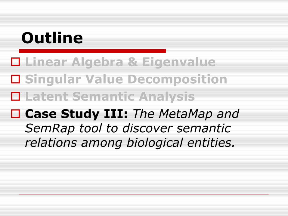
Outline
Linear Algebra & Eigenvalue
Singular Value Decomposition
Latent Semantic Analysis
Case Study III: The MetaMap and SemRap tool to discover semantic relations among biological entities.

Outline
Linear Algebra & Eigenvalue
Singular Value Decomposition
Latent Semantic Analysis
Case Study III: The MetaMap and SemRap tool to discover semantic relations among biological entities.

HZAU, [email protected]
Introduction to Information Retrieval
Eigenvalues & Eigenvectors
Eigenvectors (for a square m×m matrix S)
How many eigenvalues are there at most?
only has a non-zero solution if
This is a mth order equation in λ which can have at
most m distinct solutions (roots of the characteristic
polynomial) – can be complex even though S is real.
eigenvalue(right) eigenvector
Example
HZAU, [email protected]
Introduction to Information Retrieval
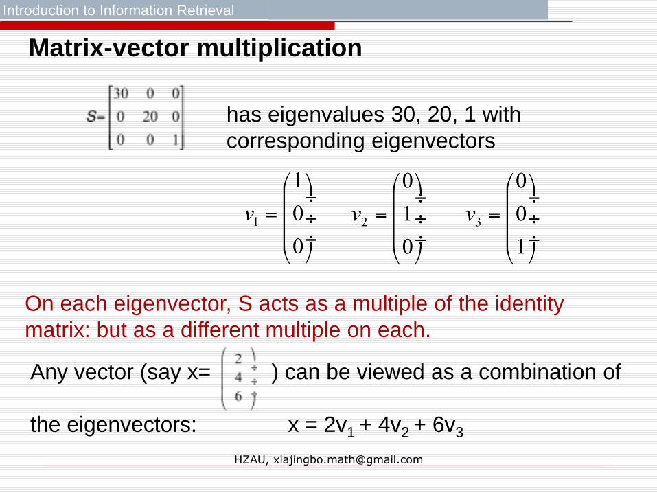
Matrix-vector multiplication
has eigenvalues 30, 20, 1 with
corresponding eigenvectors
On each eigenvector, S acts as a multiple of the identity
matrix: but as a different multiple on each.
Any vector (say x= ) can be viewed as a combination of
the eigenvectors: x = 2v1 + 4v2 + 6v3

HZAU, [email protected]
Introduction to Information Retrieval
Matrix-vector multiplication
Thus a matrix-vector multiplication such as Sx(S, x as in the previous slide) can be rewritten in terms of the eigenvalues/vectors:
Even though x is an arbitrary vector, the action of S on x is determined by the eigenvalues/vectors.

HZAU, [email protected]
Introduction to Information Retrieval
Matrix-vector multiplication
Suggestion: the effect of “small” eigenvalues is small.
If we ignored the smallest eigenvalue (1), then instead of
we would get
These vectors are similar (in cosine similarity, etc.)

HZAU, [email protected]
Introduction to Information Retrieval
Eigenvalues & Eigenvectors
For symmetric matrices, eigenvectors for distinct
eigenvalues are orthogonal
All eigenvalues of a real symmetric matrix are real.
All eigenvalues of a positive semidefinite matrix
are non-negative

HZAU, [email protected]
Introduction to Information Retrieval
Example
Let
Then
The eigenvalues are 1 and 3 (nonnegative, real).
The eigenvectors are orthogonal (and real):
Real, symmetric.
Sec. 18.1

HZAU, [email protected]
Introduction to Information Retrieval
Let be a square matrix with m
linearly independent eigenvectors
Theorem: Exists an eigen decomposition
(cf. matrix diagonalization theorem)
Columns of U are the eigenvectors of S
Diagonal elements of are eigenvalues of
Eigen/diagonal Decomposition
diagonal
Sec. 18.1
HZAU, [email protected]
Introduction to Information Retrieval
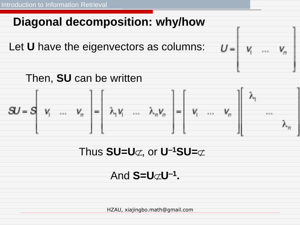
Diagonal decomposition: why/how
Let U have the eigenvectors as columns:
Then, SU can be written
And S=UU–1.
Thus SU=U, or U–1SU=

HZAU, [email protected]
Introduction to Information Retrieval
Diagonal decomposition - example
Recall
The eigenvectors and form
Inverting, we have
Then, S=UU–1 =

HZAU, [email protected]
Introduction to Information Retrieval
Example continued
Let’s divide U (and multiply U–1) by
Then, S=
(Q-1= QT )
Sec. 18.1

HZAU, [email protected]
Introduction to Information Retrieval
If is a symmetric matrix:
Theorem: There exists a (unique) eigen decomposition
where Q is orthogonal: S=QΛQT
Q-1= QT
Columns of Q are normalized eigenvectors
Columns are orthogonal.
(everything is real)
Symmetric Eigen Decomposition

HZAU, [email protected]
Introduction to Information Retrieval
Time out!
I came to this class to learn about text retrieval and mining, not to have my linear algebra past dredged up again …
What do these matrices have to do with text?
Recall M × N term-document matrices …
But everything so far needs square matrices – so …
HZAU, [email protected]
Introduction to Information Retrieval
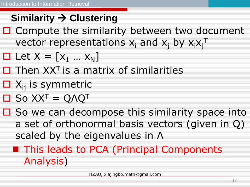
Similarity Clustering
Compute the similarity between two document vector representations xi and xj by xixj
T
Let X = [x1 … xN]
Then XXT is a matrix of similarities
Xij is symmetric
So XXT = QΛQT
So we can decompose this similarity space into a set of orthonormal basis vectors (given in Q) scaled by the eigenvalues in Λ
This leads to PCA (Principal Components Analysis)
17

Outline
Linear Algebra & Eigenvalue
Singular Value Decomposition
Latent Semantic Analysis
Case Study III: The MetaMap and SemRap tool to discover semantic relations among biological entities.
Outline
Linear Algebra & Eigenvalue
Singular Value Decomposition
Intro of SVD
Theorem&Proof of SVD computation
Examples of SVD calculation
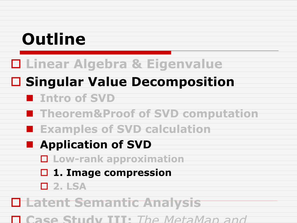
Application of SVD
Low-rank approximation
1. Image compression
2. LSA
Latent Semantic Analysis
Case Study III: The MetaMap and

Outline
Linear Algebra & Eigenvalue
Singular Value Decomposition
Intro of SVD
Theorem&Proof of SVD computation
Examples of SVD calculation
Application of SVD
Low-rank approximation
1. Image compression
2. LSA
Latent Semantic Analysis
Case Study III: The MetaMap and

HZAU, [email protected]
Introduction to Information Retrieval
Singular Value Decomposition
M×M M×N V is N×N
For an M × N matrix A of rank r there exists a
factorization (Singular Value Decomposition = SVD)
as follows:
(Proven later.)
A=UΣVT

HZAU, [email protected]
Introduction to Information Retrieval
Singular Value Decomposition
AAT = (UΣVT)(UΣVT)T = (UΣVT)(VΣUT) = UΣ2UT
M×M M×N V is N×N
The columns of U are orthogonal eigenvectors of AAT.
The columns of V are orthogonal eigenvectors of ATA.
Singular values
Eigenvalues λ1, λ2,.. λr of AAT are the eigenvalues of ATA.
σi=Sqrt(λi), Σ=diag(σ1,σ2,…,σr)
A=UΣVT

HZAU, [email protected]
Introduction to Information Retrieval
Singular Value Decomposition
Illustration of SVD dimensions and sparseness
Sec. 18.2

Outline
Linear Algebra & Eigenvalue
Singular Value Decomposition
Intro of SVD
Theorem&Proof of SVD computation
Examples of SVD calculation
Application of SVD
Low-rank approximation
1. Image compression
2. LSA
Latent Semantic Analysis
Case Study III: The MetaMap and

HZAU, [email protected]
Lemma 1
Proof: Suppose is eigenvalue of ATA,and x is the
corresponding eigenvecotor, then we have
ATAx= x.
Since ATA is symmetrical, so is a real number.
,m n T
T
Suppose A R then theeigenvaluesof A A
and AA are nonnegative.
0 ( , ) ( ) ( )
0, 0
T T
T
Ax Ax Ax Ax x x
x x
Similarly, we know eigenvalue of AAT is nonnegative.
HZAU, [email protected]
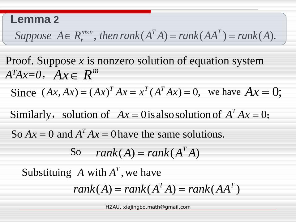
Proof. Suppose x is nonzero solution of equation system
ATAx=0,
Lemma 2
, ( ) ( ) ( ).m n T T
rSuppose A R then rank A A rank AA rank A
mAx R( , ) ( ) ( ) 0,T T TAx Ax Ax Ax x A Ax
So
Since
So 0 and 0have the same solutions.TAx A Ax
we have 0;Ax
Similarly solution of 0isalsosolution of 0TAx A Ax , ;
( ) ( ) ( )T Trank A rank A A rank AA
( ) ( )Trank A rank A A
Substituing with , we haveTA A
HZAU, [email protected]
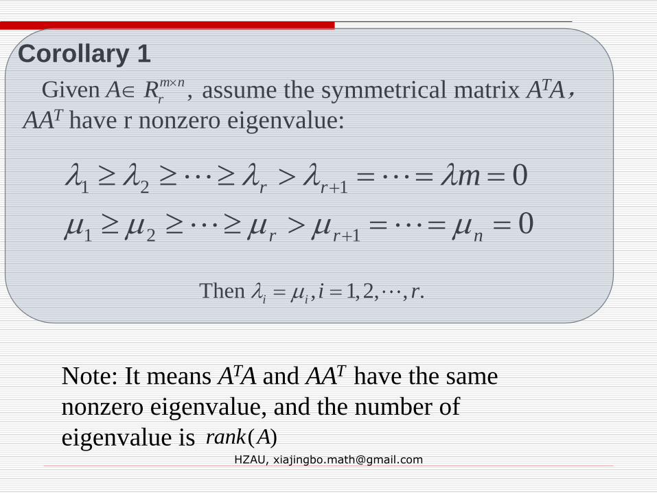
assume the symmetrical matrix ATA,AAT have r nonzero eigenvalue:
0
0
121
121
nrr
rr m
Then , 1,2, , .i i i r
Given ,m n
rA R
Note: It means ATA and AAT have the same
nonzero eigenvalue, and the number of
eigenvalue is )(Arank
Corollary 1
HZAU, [email protected]
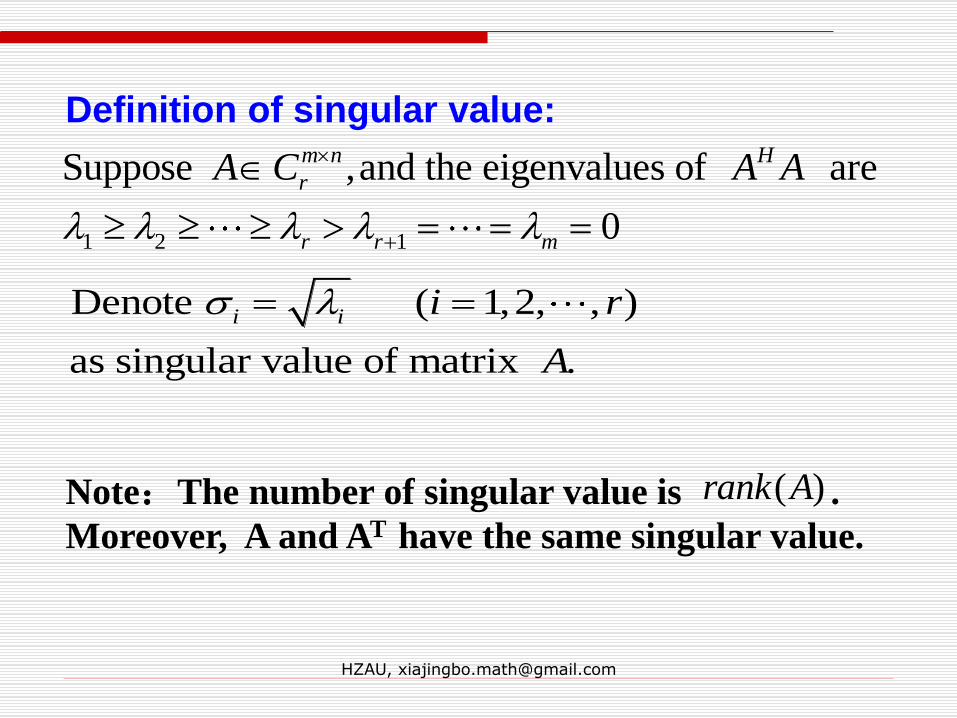
Definition of singular value:
Denote ( 1,2, , )
as singular value of matrix .
i i i r
A
1 2 1
Suppose ,and the eigenvalues of are
0
m n H
r
r r m
A C A A
Note:The number of singular value is .
Moreover, A and AT have the same singular value.
)(Arank

HZAU, [email protected]
Proof. Suppose , are orthogonally equivalent.m n
rA B R
( ) ,T T T TA A UBV UBV V B BV ( )
If two matrix are orthogonally equivalent to each other, they have the same singular values.
From
There exist orthogonal matrix , ,s.t.m m n nU C V C
A UBV
Lemma3
we know that ATA and BTB have the same eigenvalues, so do
the singular values.

HZAU, [email protected]
Formula (1) is SVD.
1 2Assume , , , , are the singular valuesm n
r rA C ,
There exisit orthogonal matrix and s.t.m m n nU V ,
0 0or (1)
0 0 0 0
T TU AV A U V
1 2Here, ( , , , )diag
Theorem of SVD !!!

HZAU, [email protected]
Proof.
)2(,00
0)(
2
VAAV HH
Since AHA is symmetrical matrix,there exist orthogonal
matrix V (rank=r), s.t.
;),,,( 222
2
2
1
2
iirdiag Here,
( )
1 2 1 2, , , ,n r n n r
r n rV V V V R V R
Splitting V, we have
And we also have:

HZAU, [email protected]
1 1 1 2
2 1 2 2
T T T T
T T T T
V A AV V A AV
V A AV V A AV
41
11
rnCAVU
2
1
1 2
2
0( ) ,
0 0
T
T
T
VA A V V
V
2
1 1 1 1
2 2 2 2
( ) ( )
( ) ( ) 0
T T T
T T T
V A AV AV AV
V A AV AV AV
Compare the left and right items, we have
3,02 AVSo we have
Denote

HZAU, [email protected]
1 2such that form an orthogonal matrix .U U U( , )
1
2 1 2 1and we have 0,H HU U U AV
1 1
1 1 1 1From 4 we have ,T T T
rU U V A AV I ( ) :
So r columns of U1 are orthogonal identical vectors.
( )
2So there exists ,m m rU C
rm
H IUU 22

HZAU, [email protected]
21
2
1 VVAU
UAVU
H
HH
Therefore,
2212
2111
AVUAVU
AVUAVUHH
HH
1
11
AVU
02 AV
,012 UU H
r
H IUU 11
0
0
12
11
UU
UUH
H
00
0
So, the theorem follows.

HZAU, [email protected]
Among the SVD result of A=UDVT,the column vectors of U are eigenvectors of AAT, while the column vectors of V are eigenvectors of ATA.
Proof. ( )( )H H H HAA UDV UDV
)0,,0,,,,()( 21
2 r
H UdiagUDUAA
HHH UUDVDUUDV 2
1 2Denote nU u u u( , , , )
we have ( ) , 1,2, ,H
i i iAA u u i n
Corollary 2

Outline
Linear Algebra & Eigenvalue
Singular Value Decomposition
Intro of SVD
Theorem&Proof of SVD computation
Examples of SVD calculation
Application of SVD
Low-rank approximation
1. Image compression
2. LSA
Latent Semantic Analysis
Case Study III: The MetaMap and

HZAU, [email protected]
1] Calculate the diagonal matrix V, which is orthogonal equivalent to AHA:
2
T 0( )
0 0
TV A A V
,,),,( )(
2121
rnnrn CVCVVVV
1
1 1 Rm rU AV
5] We get SVD:
4] Expand U1 to an orthogonal matrix U=(U1 ,U2)
3] Denote
2] Denote
SVD Algorithm 1—Using AHA
HVUA
00
0

HZAU, [email protected]
Example1、
000
110
101
A , get SVD result.
The eigenvalues are
211
110
101
AAH ,0,1,3 321
Eigenvectors are ,2,1,11
Tx ,0,1,12
Tx ,1,1,13
Tx
So we have: ,2rankA ,10
03
Let ,, 21 VVV
Here 322113
1,
2
1,
6
1xVxxV
We have 1
11 AVU
00
2
1
2
12
1
2
1

HZAU, [email protected]
By expanding TU 1,0,02
100
02
1
2
1
02
1
2
1
, 21 UUU
A ‘s SVD result is
TVUA
000
010
003

HZAU, [email protected]
Introduction to Information Retrieval
Another SVD example. Is it computable?
Let
Thus M=3, N=2. Its SVD is
Typically, the singular values arranged in decreasing order.
Sec. 18.2

Outline
Linear Algebra & Eigenvalue
Singular Value Decomposition
Intro of SVD
Theorem&Proof of SVD computation
Examples of SVD calculation
Application of SVD
Low-rank approximation
1. Image compression
2. LSA
Latent Semantic Analysis
Case Study III: The MetaMap and

HZAU, [email protected]
Introduction to Information Retrieval
SVD can be used to compute optimal low-rank approximations.
Approximation problem: Find Ak of rank k such that
Ak and X are both m×n matrices.
Typically, want k << r.
Low-rank Approximation
Frobenius norm
HZAU, [email protected]
Introduction to Information Retrieval
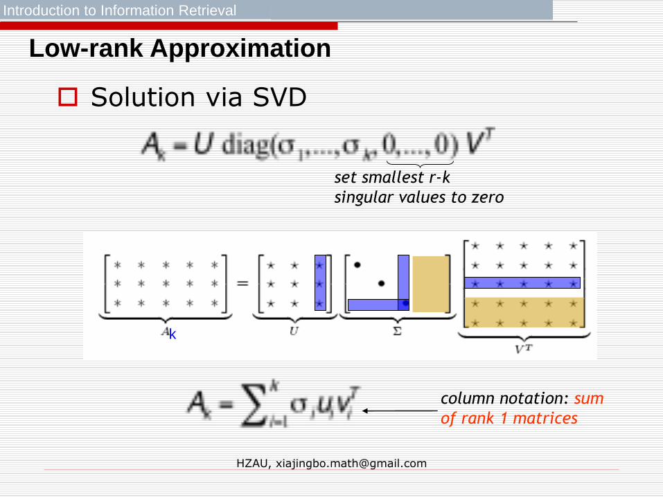
Solution via SVD
Low-rank Approximation
set smallest r-k
singular values to zero
column notation: sum
of rank 1 matrices
k
HZAU, [email protected]
Introduction to Information Retrieval
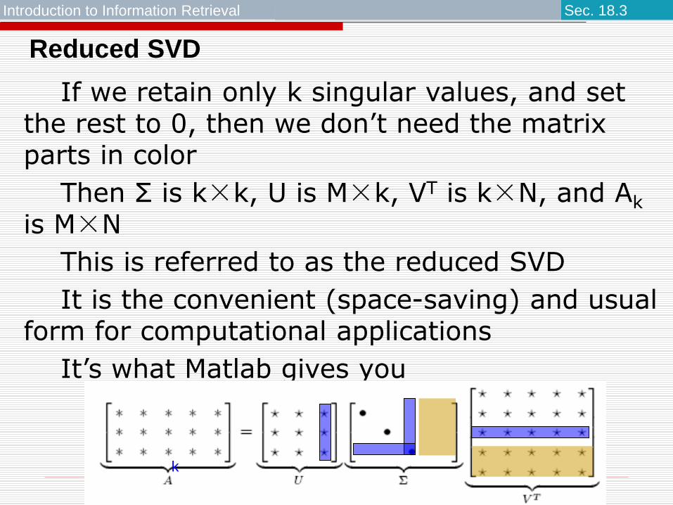
If we retain only k singular values, and set the rest to 0, then we don’t need the matrix parts in color
Then Σ is k×k, U is M×k, VT is k×N, and Ak
is M×N
This is referred to as the reduced SVD
It is the convenient (space-saving) and usual form for computational applications
It’s what Matlab gives you
Reduced SVD
k
Sec. 18.3

HZAU, [email protected]
Introduction to Information Retrieval
Approximation error
How good (bad) is this approximation?
It’s the best possible, measured by the Frobenius norm of the error:
Frobenius error drops as k increases.
Sec. 18.3

HZAU, [email protected]
Introduction to Information Retrieval
SVD Low-rank approximation
Whereas the term-doc matrix A may have M=50000, N=10 million (and rank close to 50000)
We can construct an approximation A100 with rank 100.
Of all rank 100 matrices, it would have the lowest Frobenius error.
Great … but why would we??
Answer: Image Compression
Latent Semantic Indexing
C. Eckart, G. Young, The approximation of a matrix by another of lower rank.
Psychometrika, 1, 211-218, 1936.
Outline
Linear Algebra & Eigenvalue
Singular Value Decomposition
Intro of SVD
Theorem&Proof of SVD computation
Examples of SVD calculation
Application of SVD
Low-rank approximation
1. Image compression
2. LSA
Latent Semantic Analysis
Case Study III: The MetaMap and

HZAU, [email protected]
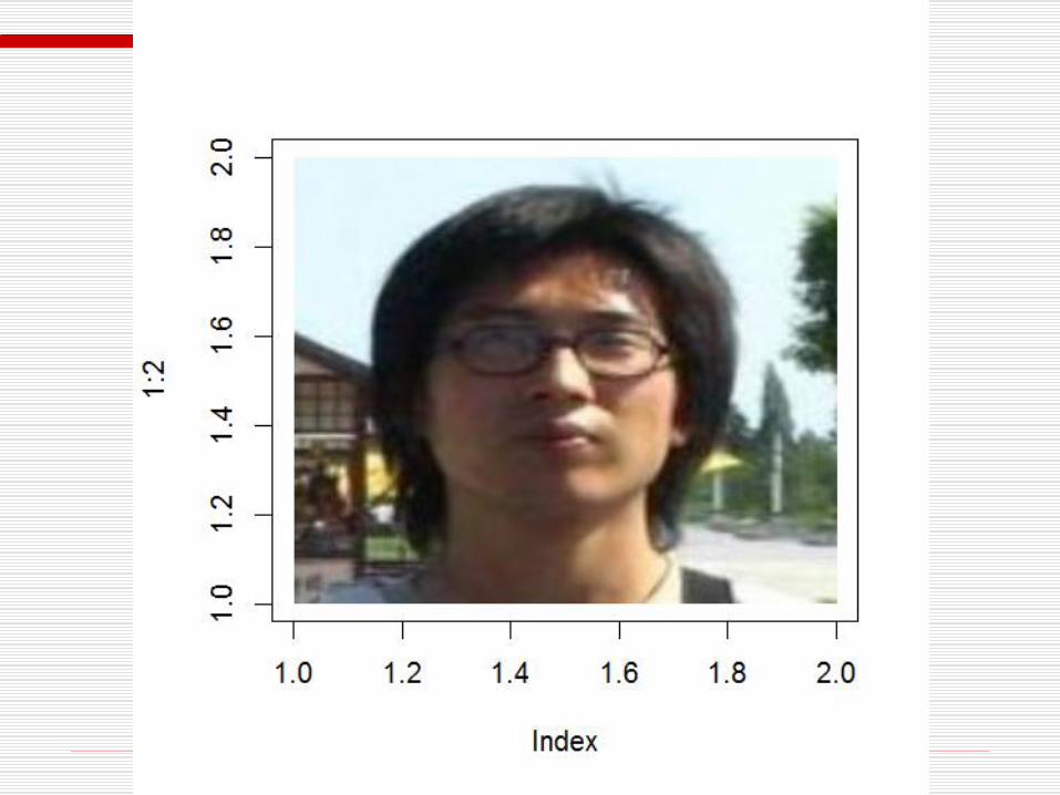
library(jpeg)
img <- readJPEG(system.file("img", “xjb.jpg", package="jpeg"))
if(exists("rasterImage")){
plot(1:2, type='n')
rasterImage(img,1,1,2,2)
}
HZAU, [email protected]

HZAU, [email protected]
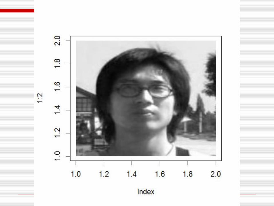
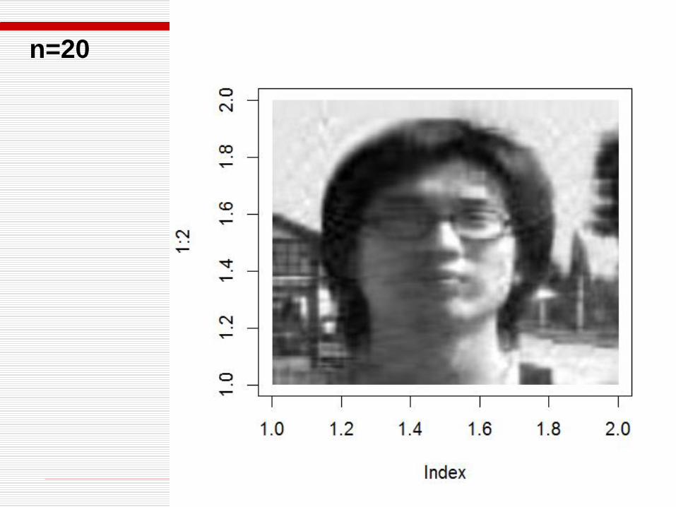
dim(img) #200*200*3
img_grey <- img[ , ,1]
dim(img_grey) #200*200
if(exists("rasterImage")){
plot(1:2, type='n')
rasterImage(img_grey,1,1,2,2)
}
HZAU, [email protected]
HZAU, [email protected]
[1] 1.069733e+02 2.919619e+01 2.205404e+01 1.689986e+01 1.326622e+01
[6] 8.760134e+00 8.373214e+00 6.950724e+00 5.907265e+00 4.979078e+00
[11] 4.717919e+00 4.288516e+00 4.127117e+00 3.861279e+00 3.502851e+00
[16] 3.053432e+00 2.676388e+00 2.546025e+00 2.414010e+00 2.184452e+00
[21] 2.084637e+00 2.038409e+00 1.881523e+00 1.751720e+00 1.683151e+00
[26] 1.575874e+00 1.447890e+00 1.429346e+00 1.322238e+00 1.268714e+00
[31] 1.259183e+00 1.180884e+00 1.127370e+00 1.044037e+00 1.012873e+00
[36] 9.528043e-01 9.002203e-01 8.669127e-01 8.185742e-01 8.048680e-01
[41] 7.719161e-01 6.900204e-01 6.863703e-01 6.444611e-01 6.223716e-01
[46] 5.690846e-01 5.593050e-01 5.431515e-01 5.317420e-01 5.035857e-01
[51] 4.857583e-01 4.663759e-01 4.522316e-01 4.359483e-01 4.154823e-01
[56] 4.039207e-01 3.862549e-01 3.718542e-01 3.448197e-01 3.439542e-01
[61] 3.274435e-01 3.149630e-01 2.963879e-01 2.894864e-01 2.858502e-01
[66] 2.645407e-01 2.500984e-01 2.384135e-01 2.315172e-01 2.262126e-01
[71] 2.187993e-01 2.051049e-01 2.038436e-01 2.020793e-01 1.900371e-01
[76] 1.852136e-01 1.842807e-01 1.756724e-01 1.654503e-01 1.602718e-01
[81] 1.562029e-01 1.496451e-01 1.445226e-01 1.378012e-01 1.323842e-01
[86] 1.286930e-01 1.257020e-01 1.211119e-01 1.162061e-01 1.140455e-01
[91] 1.080883e-01 1.057993e-01 1.040536e-01 9.989220e-02 9.837968e-02
[96] 9.446686e-02 9.148232e-02 8.795766e-02 8.631613e-02 8.345703e-02
[101] 8.081604e-02 7.613927e-02 7.497851e-02 7.120702e-02 6.759139e-02
[106] 6.648492e-02 6.577353e-02 6.163832e-02 5.996165e-02 5.869294e-02
[111] 5.769262e-02 5.621010e-02 5.402162e-02 5.267495e-02 5.113181e-02
[116] 4.910726e-02 4.754803e-02 4.568287e-02 4.507398e-02 4.392439e-02
[121] 4.231086e-02 4.124237e-02 3.774401e-02 3.683835e-02 3.527262e-02
[126] 3.404934e-02 3.203920e-02 3.173726e-02 3.039056e-02 3.001574e-02
[131] 2.931837e-02 2.862393e-02 2.829578e-02 2.749578e-02 2.727339e-02
[136] 2.664207e-02 2.531211e-02 2.511922e-02 2.444433e-02 2.374028e-02
[141] 2.339803e-02 2.258504e-02 2.234445e-02 2.178746e-02 2.143938e-02
[146] 2.033625e-02 2.021715e-02 1.999619e-02 1.911544e-02 1.860003e-02
[151] 1.824244e-02 1.790291e-02 1.750121e-02 1.662369e-02 1.636209e-02
[156] 1.609944e-02 1.561421e-02 1.468991e-02 1.418592e-02 1.401396e-02
[161] 1.350672e-02 1.342801e-02 1.307476e-02 1.239330e-02 1.202600e-02
[166] 1.176212e-02 1.104437e-02 1.092626e-02 1.016241e-02 9.735921e-03
[171] 9.407730e-03 9.071058e-03 8.682523e-03 8.443112e-03 8.130042e-03
[176] 7.843536e-03 7.400492e-03 7.283213e-03 7.046477e-03 6.360952e-03
[181] 6.159672e-03 5.855730e-03 5.574172e-03 4.951076e-03 4.789788e-03
[186] 4.419598e-03 4.103295e-03 3.874366e-03 3.214117e-03 2.994594e-03

HZAU, [email protected]
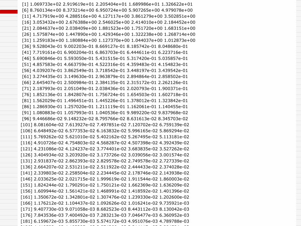
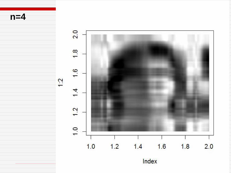
n=4
D <- diag(s$d[1:n])
img_compressed <- s$u[,1:n] %*% D %*% t(s$v[,1:n])
img_grey-img_compressed


Outline
Linear Algebra & Eigenvalue
Singular Value Decomposition
Intro of SVD
Theorem&Proof of SVD computation
Examples of SVD calculation
Application of SVD
Low-rank approximation
1. Image compression
2. LSA
Latent Semantic Analysis
Case Study III: The MetaMap and

Outline
Linear Algebra & Eigenvalue
Singular Value Decomposition
Latent Semantic Analysis
Case Study III: The MetaMap and SemRap tool to discover semantic relations among biological entities.

HZAU, [email protected]
Introduction to Information Retrieval
What it is
From term-doc matrix A, we compute the approximation Ak.
There is a row for each term and a column for each doc in Ak
Thus docs live in a space of k<<r dimensions
These dimensions are not the original axes
But why?

HZAU, [email protected]
Introduction to Information Retrieval
Vector Space Model: Pros
Automatic selection of index terms
Partial matching of queries and documents (dealing with the case where no document contains all search terms)
Ranking according to similarity score (dealing with large result sets)
Term weighting schemes (improves retrieval performance)
Various extensions
Document clustering
Relevance feedback (modifying query vector)
Geometric foundation

HZAU, [email protected]
Introduction to Information Retrieval
Problems with Lexical Semantics
Ambiguity and association in natural language
Polysemy: Words often have a multitude of meanings and different types of usage (more severe in very heterogeneous collections).
The vector space model is unable to discriminate between different meanings of the same word.
HZAU, [email protected]
Introduction to Information Retrieval
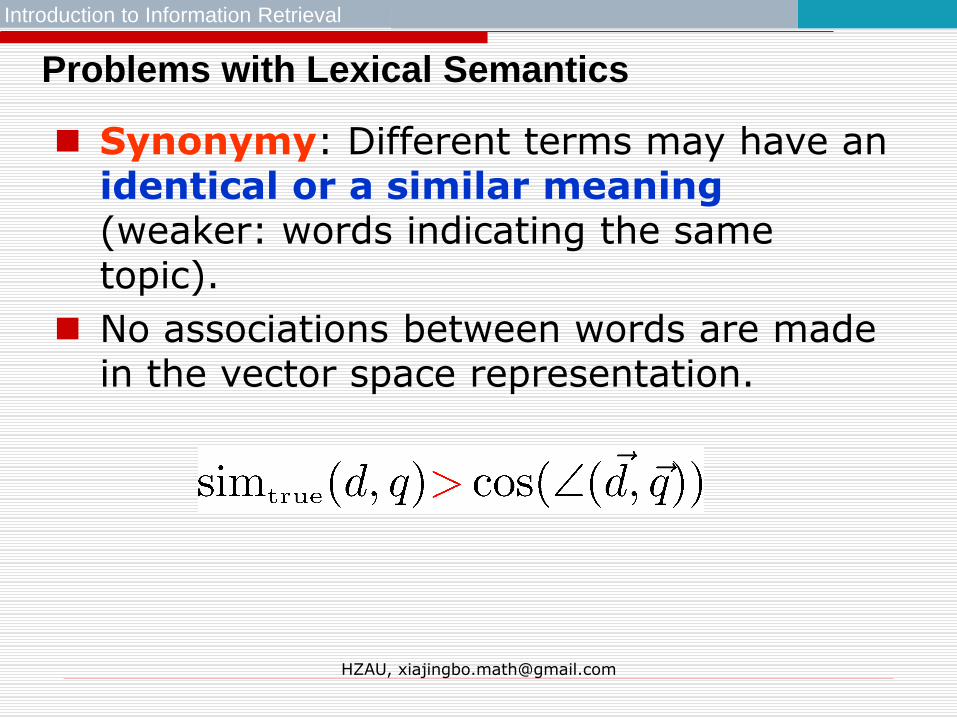
Problems with Lexical Semantics
Synonymy: Different terms may have an identical or a similar meaning(weaker: words indicating the same topic).
No associations between words are made in the vector space representation.

HZAU, [email protected]
Introduction to Information Retrieval
Polysemy and Context
Document similarity on single word level: polysemy and context
carcompany
•••dodgeford
meaning 2
ringjupiter
•••space
voyagermeaning 1…
saturn
...
…planet
...
contribution to similarity, if
used in 1st meaning, but not if
in 2nd

HZAU, [email protected]
Introduction to Information Retrieval
Latent Semantic Indexing (LSI)
Perform a low-rank approximation of document-term matrix (typical rank 100–300)
General idea
Map documents (and terms) to a low-dimensional representation.
Design a mapping such that the low-dimensional space reflects semantic associations (latent semantic space).
Compute document similarity based on the inner product in this latent semantic space

HZAU, [email protected]
Introduction to Information Retrieval
Goals of LSI
LSI takes documents that are semantically similar (= talk about the same topics), but are not similar in the vector space (because they use different words) and re-represents them in a reduced vector space in which they have higher similarity.
Similar terms map to similar location in low dimensional space
Noise reduction by dimension reduction

HZAU, [email protected]
Introduction to Information Retrieval
Latent Semantic Analysis
Latent semantic space: illustrating example
courtesy of Susan Dumais

HZAU, [email protected]
Introduction to Information Retrieval
Performing the maps
Each row and column of A gets mapped into the k-dimensional LSI space, by the SVD.
Claim – this is not only the mapping with the best (Frobenius error) approximation to A, but in fact improves retrieval.
A query q is also mapped into this space, by
Query NOT a sparse vector.
HZAU, [email protected]
Introduction to Information Retrieval
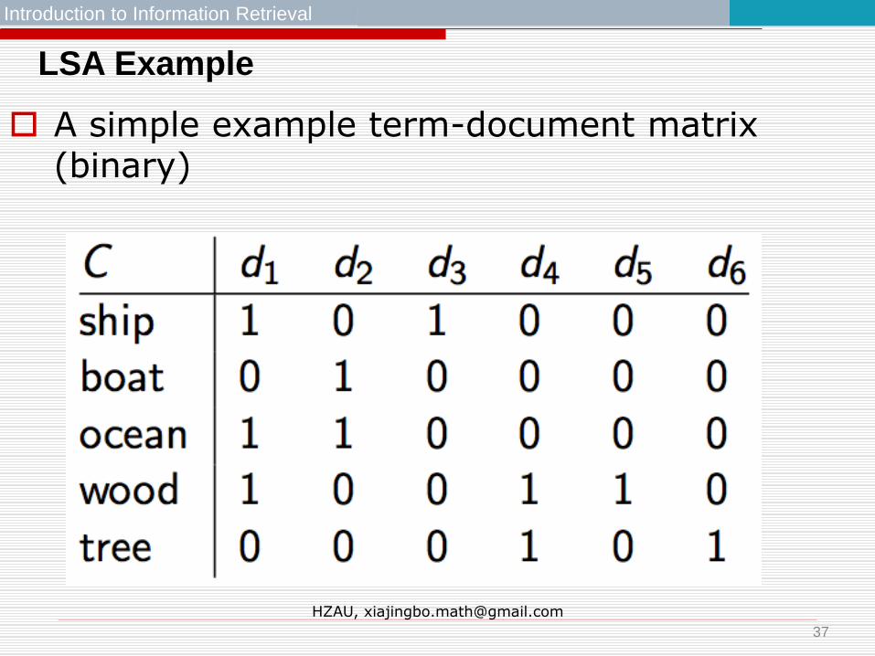
LSA Example
A simple example term-document matrix (binary)
37

HZAU, [email protected]
Introduction to Information Retrieval
LSA Example
Example of C = UΣVT: The matrix U
38

HZAU, [email protected]
Introduction to Information Retrieval
LSA Example
Example of C = UΣVT: The matrix Σ
39
HZAU, [email protected]
Introduction to Information Retrieval
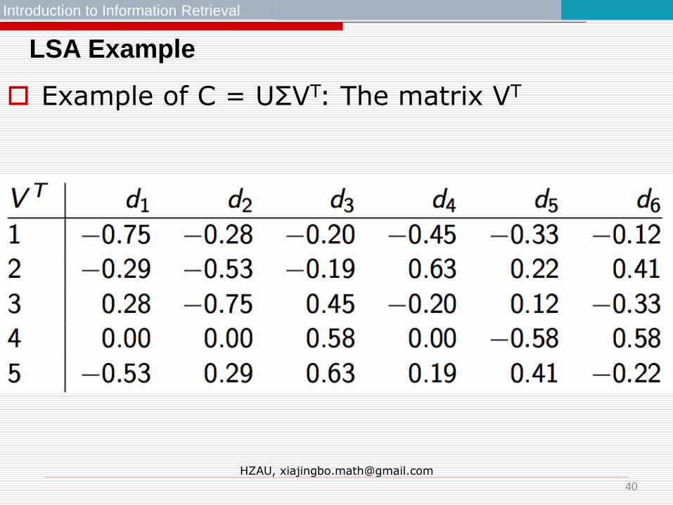
LSA Example
Example of C = UΣVT: The matrix VT
40

HZAU, [email protected]
Introduction to Information Retrieval
LSA Example: Reducing the dimension
41

HZAU, [email protected]
Introduction to Information Retrieval
Original matrix C vs. reduced C2 = UΣ2VT
42

HZAU, [email protected]
Introduction to Information Retrieval
Why the reduced dimension matrix is better
Similarity of d2 and d3 in the original space: 0.
Similarity of d2 and d3 in the reduced space: 0.52 ∗ 0.28 + 0.36 ∗ 0.16 + 0.72 ∗ 0.36 + 0.12 ∗ 0.20 + −0.39 ∗ −0.08 ≈ 0.52
Typically, LSA increases recall and hurts precision
43

HZAU, [email protected]
Introduction to Information Retrieval
LSI has many other applications
In many settings in pattern recognition and retrieval, we have a feature-object matrix.
For text, the terms are features and the docs are objects.
Could be opinions and users …
This matrix may be redundant in dimensionality.
Can work with low-rank approximation.
If entries are missing (e.g., users’ opinions), can recover if dimensionality is low.
Powerful general analytical technique
Close, principled analog to clustering methods.

HZAU, [email protected]
docs
terms D1 D2 D3 D4
disease_1 1 1 0 1
protein_a 1 0 1 2
receptor_b 1 0 0 0
atp 0 1 0 0
nadh 0 1 0 0
enzyme_c 0 0 2 0

HZAU, [email protected]
$tk
[,1] [,2]
disease_1 -0.46528933 0.49421852
protein_a -0.79793919 -0.03095791
receptor_b -0.16220124 0.15047325
atp -0.06854554 0.23775471
nadh -0.06854554 0.23775471
enzyme_c -0.33330566 -0.78682454
$dk
[,1] [,2]
D1 -0.4808393 0.3038923
D2 -0.2032006 0.4801639
D3 -0.4940359 -0.7945263
D4 -0.6952924 0.2140561
$sk
[1] 2.964462 2.019577

HZAU, [email protected]
D1 D2 D3 D4
disease_1 0.966555903 0.7595387 -0.111586760 1.1726914
protein_a 1.118406354 0.4506422 1.218297522 1.6313033
receptor_b 0.323556998 0.2436250 -0.003898531 0.3993739
atp 0.243624962 0.2718479 -0.281114472 0.2440658
nadh 0.243624962 0.2718479 -0.281114472 0.2440658
enzyme_c -0.007797061 -0.5622289 1.750687134 0.3468525
HZAU, [email protected]
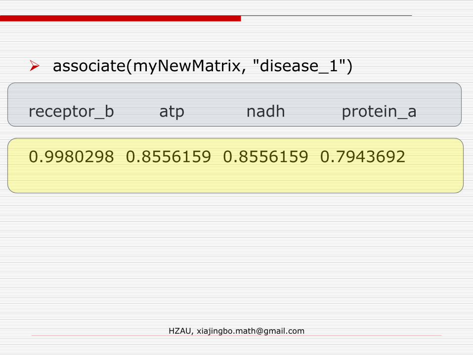
associate(myNewMatrix, "disease_1")
receptor_b atp nadh protein_a
0.9980298 0.8556159 0.8556159 0.7943692
Outline
Linear Algebra & Eigenvalue
Singular Value Decomposition
Latent Semantic Analysis
Case Study III: The MetaMap and SemRap tool to discover semantic relations among biological entities.
HZAU, [email protected]
CS276: Information Retrieval and Web Search Christopher Manning and Pandu NayakLecture 13: Latent Semantic Indexing
Reference: