7-1

CHAPTER 7 THEOREM OF SCHWARZ-CHRISTOFFEL, FREE STREAMLINES &

APPLICATIONS

Introduction The theory of free-streamlines and the theorem of Schwarz-Christoffel are presented. These are applied to flows with separation.

1. Introduction

In flow situations involving straight boundaries, the application of the theorem of Schwarz-Christoffel and of the theory free-streamlines may provide a technique to solve analytically the flow. A typical example is the flow through an orifice (Fig. 3-1A). Figure 7-1 illustrates some flow situations with separation which may be studied with the method of free streamlines. For example, the flow through a sharp orifice, the flow past a flat plate.

Remarks

1- The theory of free-streamline was introduced by Hermann HELMHOLTZ, Gustav KIRCHHOFF and others.

2- Hermann Ludwig Ferdinand von HELMHOLTZ (1821-1894) was a German scientist who made basic contributions to

physiology, optics, electrodynamics and meteorology.

3- Gustav Robert KIRCHHOFF (1824-1877) was a German physicist and mathematician who made notable

contributions to spectrum analysis, electricity, the study of light and astronomy.

Basic definitions A polygon is a closed plane figure bounded by straight lines. The term "simple closed polygon" defines a closed polygone such that : (1) the polygon boundaries divide the whole z-diagram into two regions : the interior of the polygon and the exterior; and (2) the boundaries may be completely drawn without leaving the boundary. The interior of the polygon is said to be "connected". That is, the path from any point in the interior to another point in the interior may be followed without crossing a boundary. The same may be said from the exterior region. Figure 7-2 shows simple closed polygons having vertice at infinity. The points at infinite are denoted with the subscript ∞ (e.g. A∞). Dotted arrows indicate the closure of the polygon. The interior is in white and the exterior in gray colour. Usually the polygon is drawn in the z-diagram and the interior of the polygon is the flow region.

7-2

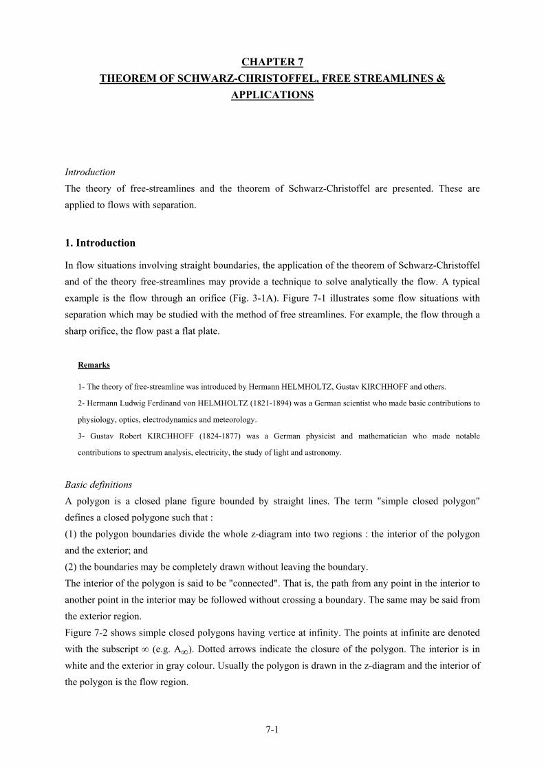
Two polygons that are often involved in problems requiring successive transformations are the semi-infinite strip and the infinite strip (Fig. 7-2). The semi-infinite strip is a rectangle with two vertices at infinity. The infinite strip a rectangle with two vertices at +∞ and two vertices at -∞. Fig. 7-1 - Flows situations with separation

Orifice flow

Sluicegate

Flow past a flat platewith separation

Flow past an objectwith separation

Flow out ofa nozzle

Notes

1- A polygon is a closed plane figure bounded by straight lines. The word derives from the Greek name polygonon for

polygon or polygonos for polygonal.

2- A vertex (plural vertices) is a point of a polygon that terminates a line or comprises the intersection of two or more

lines.

7-3

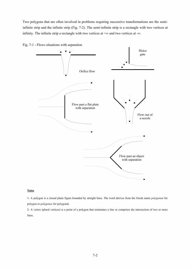
Fig. 7-2 - Simple closed polygons

Infinite strip

Semi-infinite strip

Ao o

Ao o

Ao o

Ao o

Ao o

Bo o

B

B

Bo o

Bo o

Co o

C

Co o

Co o

Do o

Do o

Do o

Upper planeis the interior

Triangle withvertices at infinity

Semi-infinite straight linewith the total planebeing the exterior

2. Theorem of Schwarz-Christoffel

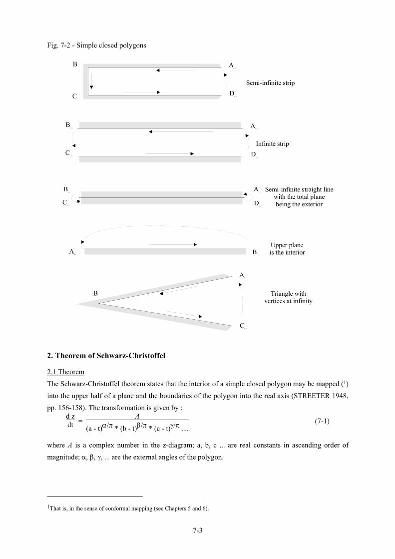
2.1 Theorem The Schwarz-Christoffel theorem states that the interior of a simple closed polygon may be mapped (1) into the upper half of a plane and the boundaries of the polygon into the real axis (STREETER 1948, pp. 156-158). The transformation is given by :

d zdt =

A

(a - t)α/π * (b - t)β/π * (c - t)γ/π .... (7-1)

where A is a complex number in the z-diagram; a, b, c ... are real constants in ascending order of magnitude; α, β, γ, ... are the external angles of the polygon.

1That is, in the sense of conformal mapping (see Chapters 5 and 6).

7-4

Notes

1- Hermann Amandus SCHWARZ was a German mathematician.

2- Elwin Bruno CHRISTOFFEL was a German mathematician who worked actively during the second half of the 19th

century.

3- In Equation (7-1), the number of real constants (a, b, c ...) and of angles (α, β, γ, ...) equals the number of vertices of

the polygon.

4- By simple geometry, the external angles of the polygon satisfy :

α + β + γ + .... = 2 * π

A polygon with four vertices is sketched in the t-diagram and in the z-diagram respectively in Figures 7-3 and 7-4. For that polygon, the theorem of Schwarz-Chritoffel implies that the transformation from the t-diagram to the z-diagram is given by :

d zdt =

A

(a - t)α/π * (b - t)β/π * (c - t)γ/π * (d - t)δ/π

For t real and t < a, the terms (a - t), (b - t) , (c - t) and (d - t) are all reals (Fig. 7-3), and the argument of dz/dt equals the argument of the complex number A. The straight line [t < a] in the t-diagram is transformed into a straight line in the z-diagram because dz = k * A * dt t < a

where k is a real. The location t = a corresponds to the vertex A. Note that dz/dt is not defined at t = a, b, c and d (Eq. (7-1)). The points A, B, C and D must be excluded from the boundaries. For t real and a < t < b, the term 1/(a - t)α/π becomes complex because (a - t) is negative and α < π. In the t-diagram, (a - t) is defined as :

a - t = r' * ei*π t > a

where r' is the modulus of (a - t). Hence :

1

(a - t)α/π = = 1

r'α/π * e-i*α t > a (7-2)

In the z-diagram, the argument of the term 1/(a - t)α/π is the angle (-α). That is, the straight line [a < t < b], in the t-diagram, transforms into a straight line in the the z-diagram and the deflection angle at the point A is equal to α since :

dz = k' * A * e-i*α * dt t < a

where k' is a real. The reasoning may be extended to the segments b < t < c, c < t < d and t > d (Fig. 7-3 & 7-4).

7-5

Fig. 7-3 - Polygon in the t-diagram

t = a

Point A

Interior of the polygon

Exterior ofthe polygonPoint B Point C Point D

t = b t = c t = d

Fig. 7-4 - Polygon from the z-diagram

y

Exterior of thepolygon

Interior of thepolygon

A B

C

γ

π−γ

βπ−β

α

π−α

δ π−δ

D

x

The integration of Equation (7-1) yields :

z = A *

⌡⌠ 1

(a - t)α/π * (b - t)β/π * (c - t)γ/π .... * dt + B (7-3)

where A and B are complex constants. The complex number A affects the scale and orientation of the polygon in the z-diagram while the complex number B determines the location of the polygon with respect to the orign.

Discussion

1- When the vertex of a polygon corresponds to a point at infinity in the t-diagram, Equation (7-1) becomes independent

of that point. STREETER (1948, pp. 162-163) and VALLENTINE (1969, p. 195) derived the proof.

For example, for a semi-infinite strip (Fig. 7-5), Equation (7-1) becomes:

d zdt =

A

(b - t)β/π * (c - t)γ/π

The points A∞ and D∞ do not contribute to the transformation because they are at infinity.

7-6

2- In Equation (7-3), the modulus of the complex number A affects the scale of the polygon and its argument determines

the polygon orientation.

3- Practically, three of the real numbers a, b, c, d, ... may be selected arbitrarily while the remaining ones are determined

by the shape of the polygon.

2.2 Applications

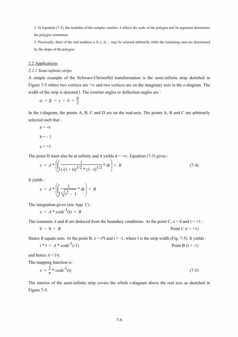
2.2.1 Semi-infinite strips A simple example of the Schwarz-Christoffel transformation is the semi-infinite strip sketched in Figure 7-5 where two vertices are +∞ and two vertices are on the imaginary axis in the z-diagram. The width of the strip is denoted l. The exterior angles or deflection angles are :

α = β = γ = δ = π2

In the t-diagram, the points A, B, C and D are on the real-axis. The points A, B and C are arbitrarily selected such that : a = -∞

b = - 1

c = +1

The point D must also be at infinity and it yields d = +∞. Equation (7-3) gives :

z = A *

⌡⌠ 1

(-(1 + t))1/2 * (1 - t)1/2 * dt + B (7-4)

It yields :

z = A *

⌡⌠ 1

t2 - 1 * dt + B

The integration gives (see App. C) : z = A * cosh-1(t) + B

The constants A and B are deduced from the boundary conditions. At the point C, z = 0 and t = +1 : 0 = 0 + B Point C (t = +1)

Hence B equals zero. At the point B, z = i*l and t = -1, where l is the strip width (Fig. 7-5). It yields : i * l = A * cosh-1(-1) Point B (t = -1)

and hence A = l/π. The mapping function is :

z = lπ * cosh-1(t) (7-5)

The interior of the semi-infinite strip covers the whole t-diagram above the real axis as sketched in Figure 7-5.

7-7

Remarks

1- In Equation (7-4), the points A∞ and D∞ do not contribute to the transformation because they are at infinity.

2- At the point B, the boundary condition yields :

cosh i * lA = -1

and hence :

cos lA = -1

since cosh(i * x) = cos(x) (see App. C). As a result, l/A = π.

Fig. 7-5 - Semi-infinite strip mapped in the z-diagram and t-diagram

Ao o

B

Do o

y

x

z-diagram

l

C

Ao o

Bb

t = -1

Do o

t-diagram

Cc

t = +1

Discussion

Figure 7-5 illustrates the simple case where C is at the origin and B is on the imaginary axis in the z-diagram. Figure 7-6

presents further examples of semi-infinite strips.

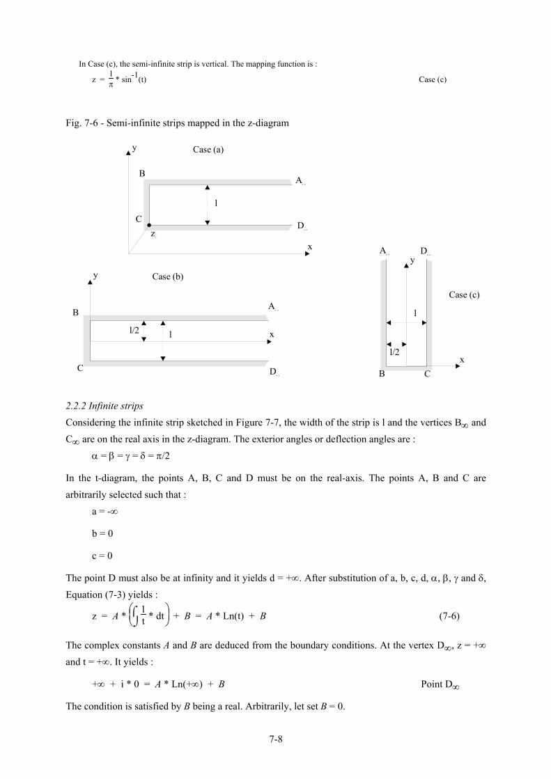
In Case (a), the mapping function is :

z = lπ * cosh-1(t) + zC Case (a)

where zC is the location of the point C in the z-diagram and l is the strip width.

In Case (b), the strip axis is the real axis in the z-diagram. It is an application of the case (a) for zC = -i*l/2. The mapping

function is :

z = lπ * cosh-1(t) - i *

l2 Case (b)

7-8

In Case (c), the semi-infinite strip is vertical. The mapping function is :

z = lπ * sin-1(t) Case (c)

Fig. 7-6 - Semi-infinite strips mapped in the z-diagram

Ao o

B

Do o

y

x

l

Cz

C

Case (a)

Ao oB

Do o

y

xl

C

Case (b)

l/2

Ao o D

o o

y

x

l

Case (c)

B C

l/2

2.2.2 Infinite strips Considering the infinite strip sketched in Figure 7-7, the width of the strip is l and the vertices B∞ and C∞ are on the real axis in the z-diagram. The exterior angles or deflection angles are : α = β = γ = δ = π/2

In the t-diagram, the points A, B, C and D must be on the real-axis. The points A, B and C are arbitrarily selected such that : a = -∞

b = 0

c = 0

The point D must also be at infinity and it yields d = +∞. After substitution of a, b, c, d, α, β, γ and δ, Equation (7-3) yields :

z = A *

⌡⌠1

t * dt + B = A * Ln(t) + B (7-6)

The complex constants A and B are deduced from the boundary conditions. At the vertex D∞, z = +∞ and t = +∞. It yields :

+∞ + i * 0 = A * Ln(+∞) + B Point D∞

The condition is satisfied by B being a real. Arbitrarily, let set B = 0.

7-9

At the vertex A∞, z = +∞ + i*l and t = -∞. It yields :

+∞ + i * l = A * Ln(-∞) = A * (+∞ + i * π) Point A∞

The boundary condition is satisfied for A = l/π. The mapping function of the infinite strip sketched in Figure 7-7 is then :

z = lπ * Ln(t) (7-7)

Fig. 7-7 - Infinite strip mapped in the z-diagram and t-diagram

z-diagramy

l

x

Ao o

Bo o

Co o D

o o

M

Ao o

b = c = 0

Do o

t-diagram

Bo o

Co o

M

Remarks

1- The constant B may be deduced from a different manner. Considering the point on the boundary C∞-D∞ such that t =

1, Equation (7-6) yields :

x = A * Ln(1) + B = 0 + B

Hence B must be a real constant. If the origin in the z-diagram (i.e. z = 0) corresponds to t = 1, then B = 0.

2- If the infinite strip is displaced vertically by a distance i*Y from the position shown in Figure 7-7, the mapping

function becomes :

z = lπ * Ln(t) + i * Y

Application : uniform flow in an infinite strip

An uniform flow in an infinite strip may be modelled by an infinite strip with a source (+q) at -∞ and a sink of equal and

opposite strength (-q) located at +∞ (Fig. 7-8). The uniform flow velocity is V = q/l where l is the strip width. In the t-

diagram, the corresponding flow pattern is located in the upper-half of the t-diagram with the source located at the origin:

7-10

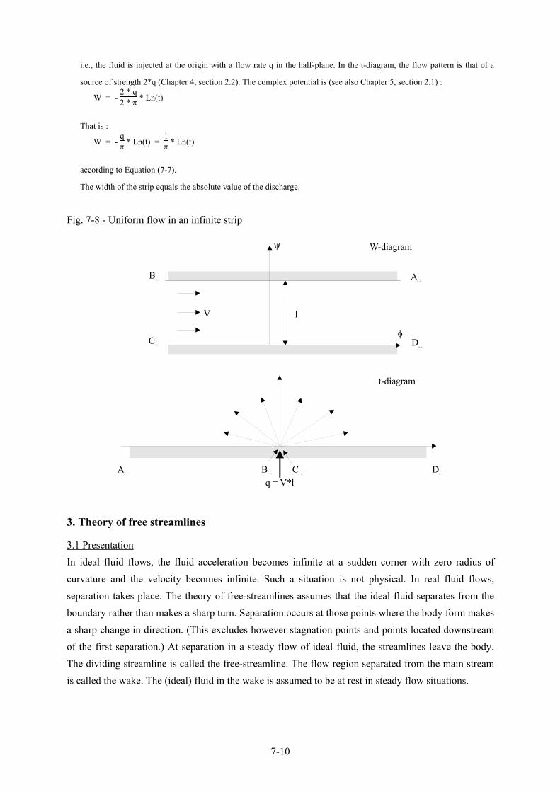
i.e., the fluid is injected at the origin with a flow rate q in the half-plane. In the t-diagram, the flow pattern is that of a

source of strength 2*q (Chapter 4, section 2.2). The complex potential is (see also Chapter 5, section 2.1) :

W = - 2 * q2 * π * Ln(t)

That is :

W = - qπ * Ln(t) =

lπ * Ln(t)

according to Equation (7-7).

The width of the strip equals the absolute value of the discharge.

Fig. 7-8 - Uniform flow in an infinite strip

q = V*lA

o oD

o o

t-diagram

Bo o

Co o

W-diagramψ

V l

φ

Ao o

Bo o

Co o D

o o

3. Theory of free streamlines

3.1 Presentation In ideal fluid flows, the fluid acceleration becomes infinite at a sudden corner with zero radius of curvature and the velocity becomes infinite. Such a situation is not physical. In real fluid flows, separation takes place. The theory of free-streamlines assumes that the ideal fluid separates from the boundary rather than makes a sharp turn. Separation occurs at those points where the body form makes a sharp change in direction. (This excludes however stagnation points and points located downstream of the first separation.) At separation in a steady flow of ideal fluid, the streamlines leave the body. The dividing streamline is called the free-streamline. The flow region separated from the main stream is called the wake. The (ideal) fluid in the wake is assumed to be at rest in steady flow situations.

7-11

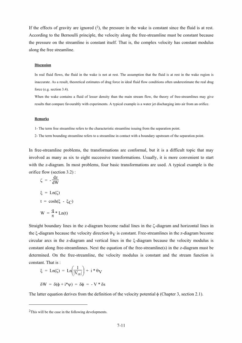
If the effects of gravity are ignored (2), the pressure in the wake is constant since the fluid is at rest. According to the Bernoulli principle, the velocity along the free-streamline must be constant because the pressure on the streamline is constant itself. That is, the complex velocity has constant modulus along the free streamline.

Discussion

In real fluid flows, the fluid in the wake is not at rest. The assumption that the fluid is at rest in the wake region is

inaccurate. As a result, theoretical estimates of drag force in ideal fluid flow conditions often underestimate the real drag

force (e.g. section 3.4).

When the wake contains a fluid of lesser density than the main stream flow, the theory of free-streamlines may give

results that compare favourably with experiments. A typical example is a water jet discharging into air from an orifice.

Remarks

1- The term free streamline refers to the characteristic streamline issuing from the separation point.

2- The term bounding streamline refers to a streamline in contact with a boundary upstream of the separation point.

In free-streamline problems, the transformations are conformal, but it is a difficult topic that may involved as many as six to eight successive transformations. Usually, it is more convenient to start with the z-diagram. In most problems, four basic transformations are used. A typical example is the orifice flow (section 3.2) :

ζ = - dz

dW

ξ = Ln(ζ)

t = cosh(ξ - ξC)

W = qπ * Ln(t)

Straight boundary lines in the z-diagram become radial lines in the ζ-diagram and horizontal lines in the ξ-diagram because the velocity direction θV is constant. Free-streamlines in the z-diagram become circular arcs in the z-diagram and vertical lines in the ξ-diagram because the velocity modulus is constant along free-streamlinnes. Next the equation of the free-streamline(s) in the z-diagram must be determined. On the free-streamline, the velocity modulus is constant and the stream function is constant. That is :

ξ = Ln(ζ) = Ln

1

|V∞| + i * θV

δW = δ(φ + i*ψ) = δφ = - V * δs

The latter equation derives from the definition of the velocity potential φ (Chapter 3, section 2.1).

2This will be the case in the following developments.

7-12

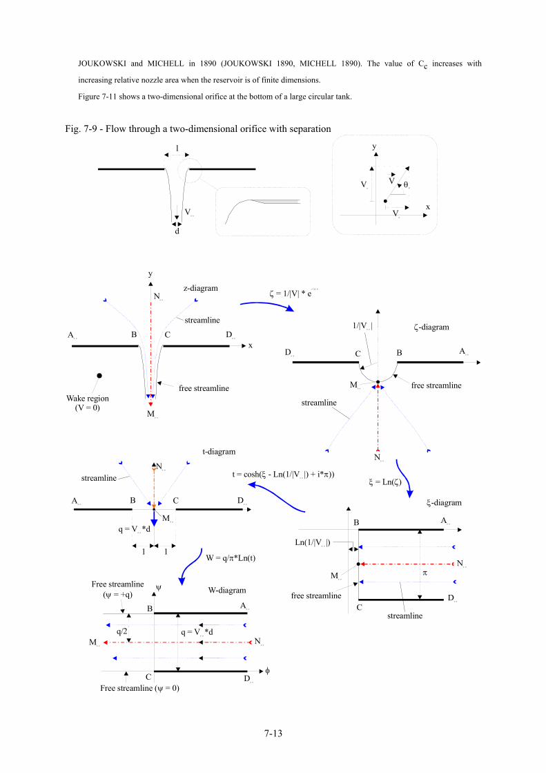
These transformations and the equations of free-streamlines are detailed for the flow through an orifice with separation and further examples. 3.2 Flow through an orifice with separation Considering a two-dimensional orifice at the bottom of a infinitely large tank, the orifice has a length l. Downstream of the orifice, the free jet thickness tends to d and the jet velocity at infinity is V∞ (Fig. 7-9). By continuity, the flow rate is q = V∞*d. At the orifice edges, separation must occur : i.e., points B and C in Figure 7-9. The problem is to find the profile of the free streamline. Along the free-streamline, the velocity is constant and it equals the jet velocity at infinity V∞. The conformal transformation consists of several successive simple transformations sketched in Figures 7-12 to 7-15.

Discussion

Orifice flows were used as water clock, called clepsydra, in ancient Babylon and Egypt (3) as well as in parts of Africa

and by some North America Indians (Fig. 7-10). They were in use up to the 16-th century. Today the sand glass (4) uses

the same principle with granular material. Orifices and nozzles are used also as measuring discharges. In his study of

orifice flows, J.C. de BORDA (1733-1799) made a significant contribution by not only introducing the concept of

streamlines but also by developing the "Borda" mouthpiece to measure accurately the orifice flow. A related form of

orifice is the sharp-crested weir commonly used for discharge measurement in open channels (e.g. CHANSON 1999, pp.

322-323).

When waters flow through a sharp-edged orifice, the jet flow contracts to have its smallest section a small distance

downstream of the hole. For a horizontal jet, Bernoulli principle implies that the velocity at vena contracta (i.e. V∞)

equals 2*g*H where H is the reservoir head above orifice centreline (Fig. 7-16). This relationship is called Torricelli

theorem, after Evangelista TORRICELLI (1608-1647) who discovered it in 1643. By continuity, the orifice discharge

equals:

Q = Cd * Ao * 2 * g * H

where Ao is the orifice cross-section area. The discharge coefficient Cd may be expressed as:

Cd = Cc*Cv

where the velocity coefficient Cv account for the energy losses and the contraction coefficient Cc equals A/Ao, A being

the jet cross-section area at vena contracta. For a water jet discharging horizontally from an infinite reservoir, Cc equals

0.58 and 0.61 for axisymmetrical and two-dimensional jets respectively (5). For example, HUNT (1968) for

axisymmetrical jets and MISES (1917) for two-dimensional jets. The result for round orifice was proposed first by E.

TREFFTZ. For two-dimensional jets, Cc = π/(π+2) (see next section). This result was derived independently by

3Hero of Alexandria (1st century A.D.) wrote a treaty on water clock in four books.

4For example, the egg timer.

5These results were obtained for sharp-edged orifices.

7-13

JOUKOWSKI and MICHELL in 1890 (JOUKOWSKI 1890, MICHELL 1890). The value of Cc increases with

increasing relative nozzle area when the reservoir is of finite dimensions.

Figure 7-11 shows a two-dimensional orifice at the bottom of a large circular tank.

Fig. 7-9 - Flow through a two-dimensional orifice with separation

ξ ζ= Ln( )t = cosh( - Ln(1/|V |) + i* ))ξ π

o o

ζ = 1/|V| * ei * Vθ

streamline

ξ-diagram

free streamline

Ao o

Mo o

No o

Do o

B

C

Ln(1/|V |)o o

π

W = q/ *Ln(t)π

Ao o

Mo o

No o

Do o

B

streamline

C

1 1

t-diagram

q = V *do o

free streamline

streamline

Wake region(V = 0)

Ao o

Mo o

No o

Do o

Bx

y

C

z-diagram

streamline

free streamline

Ao o

Mo o

No o

Do o BC

ζ-diagram1/|V |o o

W-diagramψ

Free streamline ( = 0)ψ

Free streamline( = +q)ψ

φ

Ao oB

C Do o

Mo o

No o

q = V *do o

q/2

l

d

Vo o

y

Vy

Vx

x

θV

V

7-14

Remarks

1- Hero of Alexandria was a Greek mathematician (1st century A.D.) working in Alexandria, Egypt. He wrote at least 13

books on mathematics, mechanics and physics. He designed and experimented the first steam engine. His treatise

"Pneumatica" described Hero's fountain, siphons, steam-powered engines, a water organ, and hydraulic and mechanical

water devices. It influenced directly the waterworks design during the Italian Renaissance. In his book "Dioptra", HERO

stated rightly the concept of continuity for incompressible flow : the discharge being equal to the area of the cross-

section of the flow times the speed of the flow.

2- Evangelista TORRICELLI (1608-1647) was an Italian physicist and mathematician who invented the barometer. From

1641 TORRICELLI worked with the elderly astronomer GALILEO and was later appointed to succeed him as professor

of mathematics at the Florentine Academy.

Fig. 7-10 - Clepsydra (water clock) - The Clepsydra is equipped with a circular orifice at the bottom of the tank (A) Sketch

(B) Section shape of a clepsydra : orifice diameter = 4 mm, emptying time = 23 hours

0

0.1

0.2

0.3

0.4

0.5

0.6

0.7

0.8

-1 -0.8 -0.6 -0.4 -0.2 0 0.2 0.4 0.6 0.8 1

r (m)

H (m)

7-15

Fig. 7-11 - Photograph of the free-falling jet beneath a large two-dimensional orifice flow (l = 0.070 m, B = 0.750 m) at the bottom of a large circular tank (CHANSON et al. 2002) - Frontal view of the full jet width (0.750 m)

Transformation from z-diagram to ζ-diagram The transformation is defined as :

ζ = - dz

dW (7-8)

where W is the complex potential (Chapter 5). Basically ζ is the inverse of the complex velocity :

ζ = - 1

- Vx + i * Vy =

1|V| * ei * θV

where |V| is the modulus of the local velocity and θV is the local velocity direction (6), also called the argument of the velocity vector in the z-diagram (Chapter 5, section 1.3). In the z-diagram, straight boundaries are streamlines because all solid boundaries are streamlines. In the ζ-diagram, straight solid boundaries become radial lines. In the z-diagram, the velocity modulus and flow direction at the point A∞ are 0 and 0 respectively. In the ζ-diagram, the point A∞ is also

6That is, θV is the angle of the velocity vector with the horizontal real axis in the z-diagram.

7-16

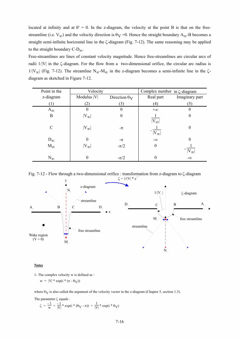
located at infinity and at θ' = 0. In the z-diagram, the velocity at the point B is that on the free-streamline (i.e. V∞) and the velocity direction is θV =0. Hence the straight boundary A∞-B becomes a straight semi-infinite horizontal line in the ζ-diagram (Fig. 7-12). The same reasoning may be applied to the straight boundary C-D∞. Free-streamlines are lines of constant velocity magnitude. Hence free-streamlines are circular arcs of radii 1/|V| in the ζ-diagram. For the flow from a two-dimensional orifice, the circular arc radius is 1/|V∞| (Fig. 7-12). The streamline N∞-M∞ in the z-diagram becomes a semi-infinite line in the ζ-diagram as sketched in Figure 7-12.

Point in the Velocity Complex number in ζ-diagram z-diagram Modulus |V| Direction θV Real part Imaginary part

(1) (2) (3) (4) (5) A∞ 0 0 +∞ 0 B |V∞| 0 1

|V∞| 0

C |V∞| -π - 1

|V∞| 0

D∞ 0 -π -∞ 0 M∞ |V∞| -π/2 0

- 1

|V∞|

N∞ 0 -π/2 0 -∞

Fig. 7-12 - Flow through a two-dimensional orifice : transformation from z-diagram to ζ-diagram

ζ = 1/|V| * ei * Vθ

free streamline

streamline

Wake region(V = 0)

Ao o

Mo o

No o

Do o

Bx

y

C

z-diagram

streamline

free streamline

Ao o

Mo o

No o

Do o BC

ζ-diagram1/|V |o o

Notes

1- The complex velocity w is defined as :

w = |V| * exp(i * (π - θV))

where θV is also called the argument of the velocity vector in the z-diagram (Chapter 5, section 1.3).

The parameter ζ equals :

ζ = - 1w =

- 1|V| * exp(i * (θV - π)) =

1|V| * exp(i * θV)

7-17

since exp(i*(x - π)) = exp(i*(x + π)) = - exp(i*x).

2- At the orifice edges (points B and C), the flow cannot turn sharply and separation must occur. The fluid leaves the

orifice edge in the tangential direction as sketched in Fig. 7-9.

3- Calculations are conducted neglecting gravity effects.

4- During the mapping of the z-diagram into the ζ-diagram, the upper half of the plane in the z-diagram (i.e. flow

upstream of orifice) becomes the lower half of the plane in the ζ-diagram (i.e. beneath the circular arc). For example, see

the transformation of the streamlines N∞-M∞. Few further streamlines are shown in Figure 7-12. In the ζ-diagram, all

the streamlines converge to the point M∞ because the velocity downstream of orifice and at infinity tends to :

V = V∞*e-i*π/2.

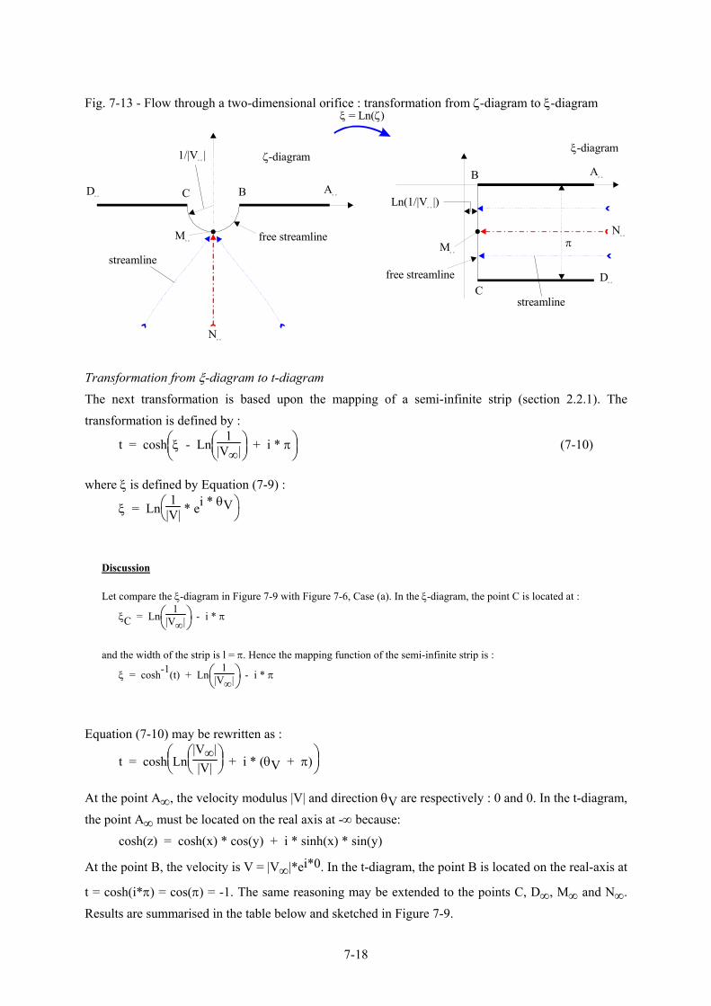
Transformation from ζ-diagram to ξ-diagram The transformation is defined by : ξ = Ln(ζ) (7-9a)

where ζ is defined by Equation (7-8). It may be rewritten :

ξ = Ln

1

|V| + i * θV (7-9b)

since Ln(r*ei*θ) = Ln(r) + i*θ for 0 ≤ θ < 2*π (See App. C). Basically the real part of ξ is 1/|V| and its imaginary part is θV (i.e. local velocity direction). Straight lines in the z-diagram become radial lines in the ζ-diagram and horizontal lines in the ξ-diagram because θV is constant. At the point A∞, the velocity modulus is zero and the velocity direction is 0 in the z-diagram. The corresponding point in the ξ-diagram has an infinite real part and zero imaginary part. The same reasoning may be applied to the points B, C, D∞, M∞ and N∞. Results are summarised in the table below and sketched in Figure 7-13.

Point in the z-diagram Complex number in ξ-diagram Real part Imaginary part

(1) (2) (3) A∞ +∞ 0 B

Ln

1

|V∞| 0

C Ln

1

|V∞| -π

D∞ +∞ -π M∞

Ln

1

|V∞| -π/2

N∞ +∞ -π/2

Free-streamlines in the z-diagram become circular arcs in the z-diagram and vertical lines in the ξ-diagram because the velocity modulus is constant along free-streamlines. In the z-diagram, the velocity at the point M∞ is : |V| = |V∞| and θV = -π/2. In the ξ-diagram, the point M∞ is sketched in Figure 7-13. All streamlines becomes horizontal lines in the ξ-diagram. In the ξ-diagram, the flow field becomes a semi-infinite strip.

7-18

Fig. 7-13 - Flow through a two-dimensional orifice : transformation from ζ-diagram to ξ-diagram

ξ ζ= Ln( )

streamline

ξ-diagram

free streamline

Ao o

Mo o

No o

Do o

B

C

Ln(1/|V |)o o

πstreamline

free streamline

Ao o

Mo o

No o

Do o BC

ζ-diagram1/|V |o o

Transformation from ξ-diagram to t-diagram The next transformation is based upon the mapping of a semi-infinite strip (section 2.2.1). The transformation is defined by :

t = cosh

ξ - Ln

1

|V∞| + i * π (7-10)

where ξ is defined by Equation (7-9) :

ξ = Ln

1

|V| * ei * θV

Discussion

Let compare the ξ-diagram in Figure 7-9 with Figure 7-6, Case (a). In the ξ-diagram, the point C is located at :

ξC = Ln

1

|V∞| - i * π

and the width of the strip is l = π. Hence the mapping function of the semi-infinite strip is :

ξ = cosh-1(t) + Ln

1

|V∞| - i * π

Equation (7-10) may be rewritten as :

t = cosh

Ln

|V∞|

|V| + i * (θV + π)

At the point A∞, the velocity modulus |V| and direction θV are respectively : 0 and 0. In the t-diagram, the point A∞ must be located on the real axis at -∞ because: cosh(z) = cosh(x) * cos(y) + i * sinh(x) * sin(y)

At the point B, the velocity is V = |V∞|*ei*0. In the t-diagram, the point B is located on the real-axis at

t = cosh(i*π) = cos(π) = -1. The same reasoning may be extended to the points C, D∞, M∞ and N∞. Results are summarised in the table below and sketched in Figure 7-9.

7-19

Point in the z-diagram Complex number in t-diagram Real part Imaginary part

(1) (2) (3) A∞ -∞ 0 B -1 0 C +1 0

D∞ +∞ 0 M∞ 0 0 N∞ 0 +∞

Fig. 7-14 - Flow through a two-dimensional orifice : transformation from ξ-diagram to t-diagram

t = cosh( - Ln(1/|V |) + i* ))ξ πo o

streamline

ξ-diagram

free streamline

Ao o

Mo o

No o

Do o

B

C

Ln(1/|V |)o o

π

Ao o

Mo o

No o

Do o

B

streamline

C

1 1

t-diagram

q = V *do o

Remarks

1- Basic properties of the hyperbolic cosine function cosh are :

cosh(z) = cosh(x) * cos(y) + i * sinh(x) * sin(y)

cosh(i * x) = cos(x) cosh(x) = cos(i * x)

2- On the free streamlines, the velocity modulus is |V∞| :

t = cosh(i * (θV + π)) = cos(θV + π)

3- If the velocity at infinity downstream of the orifice V∞ = 1, Equation (7-10) may be simplified :

t = cosh( )ξ + i * π

In the t-diagram, the point M∞ becomes the origin as sketched in Figure 7-9. Note that all streamlines becomes radial lines in the upper half-plane and converging to the origin. In the t-diagram, the flow field becomes that of a half-sink at the origin. The discharge from the half-sink is q = V∞*d where d is the free-jet thickness at infinity downstream of the orifice.

Transformation from t-diagram to W-diagram The final transformation from the t-diagram to the W-diagram is basically described in section 2.2.2 :

7-20

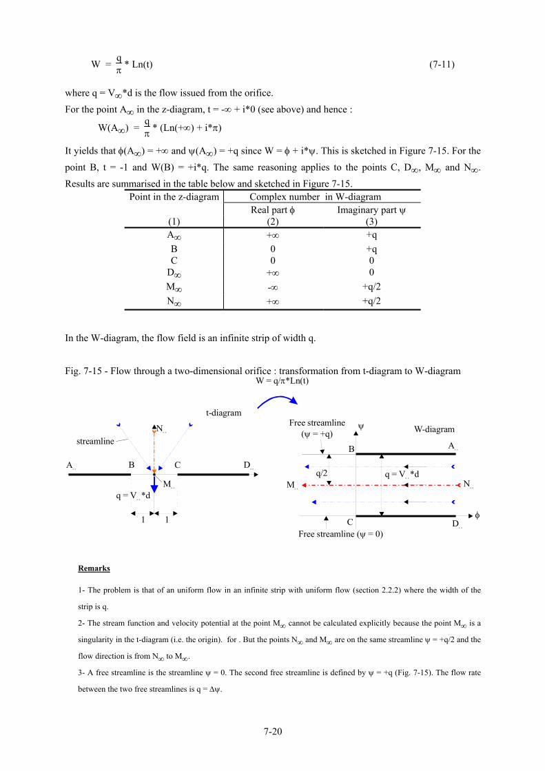
W = qπ * Ln(t) (7-11)

where q = V∞*d is the flow issued from the orifice. For the point A∞ in the z-diagram, t = -∞ + i*0 (see above) and hence :

W(A∞) = qπ * (Ln(+∞) + i*π)

It yields that φ(A∞) = +∞ and ψ(A∞) = +q since W = φ + i*ψ. This is sketched in Figure 7-15. For the point B, t = -1 and W(B) = +i*q. The same reasoning applies to the points C, D∞, M∞ and N∞. Results are summarised in the table below and sketched in Figure 7-15.

Point in the z-diagram Complex number in W-diagram Real part φ Imaginary part ψ

(1) (2) (3) A∞ +∞ +q B 0 +q C 0 0

D∞ +∞ 0 M∞ -∞ +q/2 N∞ +∞ +q/2

In the W-diagram, the flow field is an infinite strip of width q. Fig. 7-15 - Flow through a two-dimensional orifice : transformation from t-diagram to W-diagram

W = q/ *Ln(t)π

Ao o

Mo o

No o

Do o

B

streamline

C

1 1

t-diagram

q = V *do o

W-diagramψ

Free streamline ( = 0)ψ

Free streamline( = +q)ψ

φ

Ao oB

C Do o

Mo o

No o

q = V *do o

q/2

Remarks

1- The problem is that of an uniform flow in an infinite strip with uniform flow (section 2.2.2) where the width of the

strip is q.

2- The stream function and velocity potential at the point M∞ cannot be calculated explicitly because the point M∞ is a

singularity in the t-diagram (i.e. the origin). for . But the points N∞ and M∞ are on the same streamline ψ = +q/2 and the

flow direction is from N∞ to M∞.

3- A free streamline is the streamline ψ = 0. The second free streamline is defined by ψ = +q (Fig. 7-15). The flow rate

between the two free streamlines is q = ∆ψ.

7-21

Determination of the free streamlines In the W-diagram, the free streamlines are defined by ψ = 0 and +q respectively. The shape of these streamlines in the z-diagram is defined by the conformal transformation. On the free streamlines, the velocity modulus is a constant : |V| = |V∞|. Hence :

ξ = Ln(ζ) = Ln

1

|V∞| + i * θV (7-12)

and t = cosh(i * (θV + π)) = cos(θV + π) = - cos(θV) (7-13)

where θV varies from 0 to -π/2 along the free streamline B-M∞ while -π ≤ θV ≤ -π/2 on the free streamline C-M∞. The stream function is also a constant along a streamline. Hence the complex potential satisfies : δW = δ(φ + i*ψ) = δφ = - |V∞| * δs (7-14)

where s is the direction along the streamline. This equation derives from the definition of the velocity potential (Chapter 3, section 2.1). The differentiation of Equation (7-11) gives also :

δW = qπ *

δtt (7-15)

Discussion : free-jet thickness at infinity

By definition of the velocity vector angle θV, the streamwise coordinate s and the horizontal coordinate x in the z-

diagram are related by :

δx = cos(θV) * δs

Using Equations (7-14) and (7-15), it yields :

δx = cos(θV) * - q

π * |V∞| * δtt =

qπ * |V∞| * δt

Along the free-streamline B-M∞, the coordinate x increases from -l/2 to -d/2, while t increases from -1 to 0 :

⌡⌠-l/2

-d/2 dx =

l - d2 =

⌡⌠

-1

0q

π * |V∞| * dt = q

π * |V∞|

Using the continuity equation (q = |V∞|*d), this gives the contraction ratio :

dl =

ππ + 2 = 0.6110

where l is the orifice width and d is the free-jet thickness at infinity (Fig. 7-9).

The result compares well with experimental observations of two-dimensional water jets discharging into atmosphere (see

above). Note however that the calculations were conducted neglecting gravity. CHANSON et al. (2002) studied two-

dimensional jets discharging vertically downwards and their results showed some influence of the gravity force.

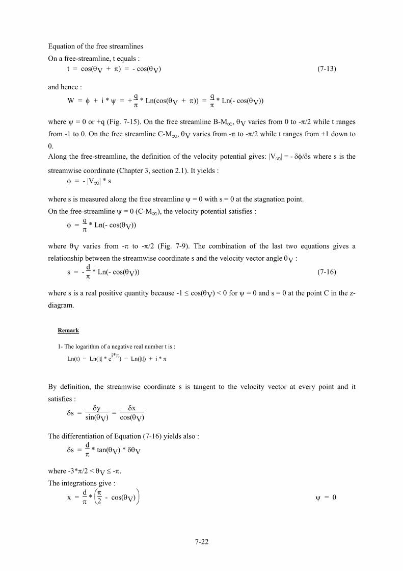
7-22

Equation of the free streamlines On a free-streamline, t equals : t = cos(θV + π) = - cos(θV) (7-13)

and hence :

W = φ + i * ψ = + qπ * Ln(cos(θV + π)) =

qπ * Ln(- cos(θV))

where ψ = 0 or +q (Fig. 7-15). On the free streamline B-M∞, θV varies from 0 to -π/2 while t ranges from -1 to 0. On the free streamline C-M∞, θV varies from -π to -π/2 while t ranges from +1 down to 0. Along the free-streamline, the definition of the velocity potential gives: |V∞| = - δφ/δs where s is the

streamwise coordinate (Chapter 3, section 2.1). It yields : φ = - |V∞| * s

where s is measured along the free streamline ψ = 0 with s = 0 at the stagnation point. On the free-streamline ψ = 0 (C-M∞), the velocity potential satisfies :

φ = qπ * Ln(- cos(θV))

where θV varies from -π to -π/2 (Fig. 7-9). The combination of the last two equations gives a relationship between the streamwise coordinate s and the velocity vector angle θV :

s = - dπ * Ln(- cos(θV)) (7-16)

where s is a real positive quantity because -1 ≤ cos(θV) < 0 for ψ = 0 and s = 0 at the point C in the z-diagram.

Remark

1- The logarithm of a negative real number t is :

Ln(t) = Ln(|t| * ei*π) = Ln(|t|) + i * π

By definition, the streamwise coordinate s is tangent to the velocity vector at every point and it satisfies :

δs = δy

sin(θV) = δx

cos(θV)

The differentiation of Equation (7-16) yields also :

δs = dπ * tan(θV) * δθV

where -3*π/2 < θV ≤ -π. The integrations give :

x = dπ *

π

2 - cos(θV) ψ = 0

7-23

y = - dπ *

Ln

- tan

θV

2 + π4 - sin(θV) ψ = 0

These are the parametric equations in terms of θV describing the free streamline C-M∞ (i.e. ψ = 0). A similar development may be conducted for the streamline B-M∞ (i.e. ψ = +q) :

x = - dπ *

π

2 + cos(θV) ψ = +q

y = dπ *

Ln

tan

θV

2 + π4 - sin(θV) ψ = +q

Discussion

In the flow downstream of an orifice with separation, the centreline streamline (i.e. N∞-M∞) may be replaced by a solid

boundary. The free-streamline then represents the case of a supercritical flow under a sluice gate.

For a horizontal flow downstream of a vertical sluice gate, experimental observations illustrated that the jet contracts to a

minimum (called vena contracta) before the developing boundary layer induces some form of flow bulking.

Experimental data showed that the vena contracta is located about 1.7 times the orifice height downstream of the orifice

(e.g. MONTES 1998, pp. 283-284).

Such a distance would correspond to y/l = -1.7 in Figure 7-9 and the contraction ratio of the free streamline at that

location is about x/(l/2) = 0.305.

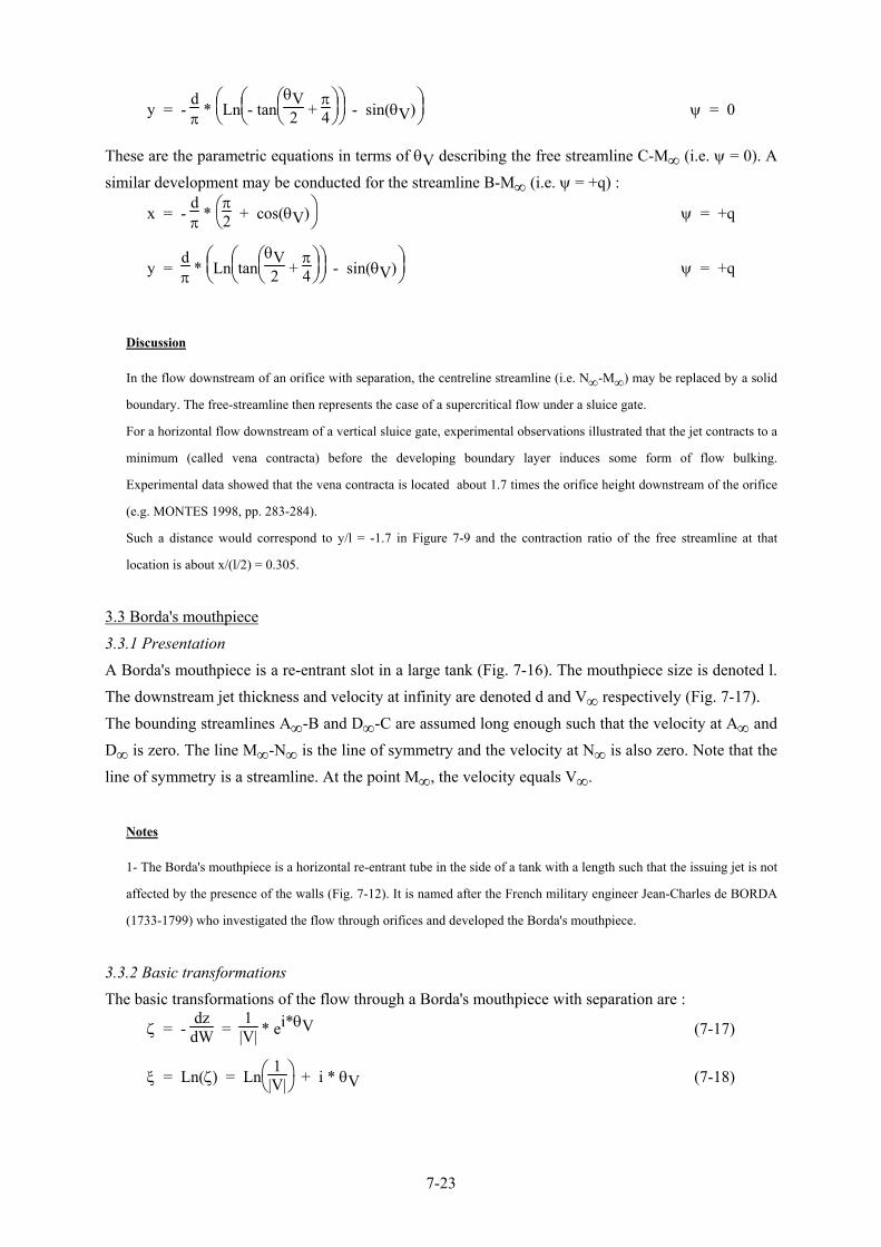
3.3 Borda's mouthpiece

3.3.1 Presentation A Borda's mouthpiece is a re-entrant slot in a large tank (Fig. 7-16). The mouthpiece size is denoted l. The downstream jet thickness and velocity at infinity are denoted d and V∞ respectively (Fig. 7-17). The bounding streamlines A∞-B and D∞-C are assumed long enough such that the velocity at A∞ and D∞ is zero. The line M∞-N∞ is the line of symmetry and the velocity at N∞ is also zero. Note that the line of symmetry is a streamline. At the point M∞, the velocity equals V∞.

Notes

1- The Borda's mouthpiece is a horizontal re-entrant tube in the side of a tank with a length such that the issuing jet is not

affected by the presence of the walls (Fig. 7-12). It is named after the French military engineer Jean-Charles de BORDA

(1733-1799) who investigated the flow through orifices and developed the Borda's mouthpiece.

3.3.2 Basic transformations The basic transformations of the flow through a Borda's mouthpiece with separation are :

ζ = - dz

dW = 1

|V| * ei*θV (7-17)

ξ = Ln(ζ) = Ln

1

|V| + i * θV (7-18)

7-24

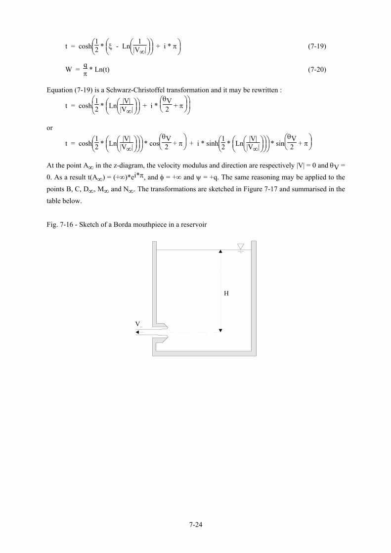
t = cosh

1

2 *

ξ - Ln

1

|V∞| + i * π (7-19)

W = qπ * Ln(t) (7-20)

Equation (7-19) is a Schwarz-Christoffel transformation and it may be rewritten :

t = cosh

1

2 *

Ln

|V|

|V∞| + i *

θV

2 + π

or

t = cosh

1

2 *

Ln

|V|

|V∞| * cos

θV

2 + π + i * sinh

1

2 *

Ln

|V|

|V∞| * sin

θV

2 + π

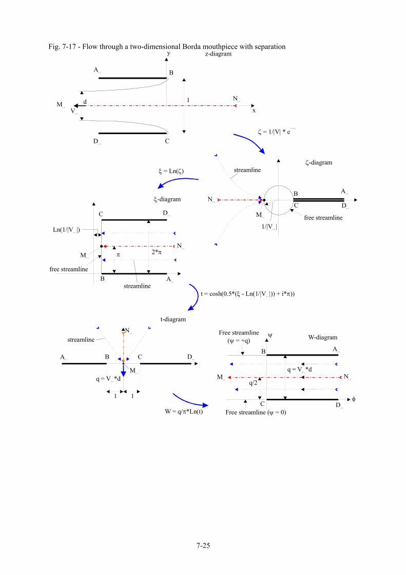
At the point A∞ in the z-diagram, the velocity modulus and direction are respectively |V| = 0 and θV = 0. As a result t(A∞) = (+∞)*ei*π, and φ = +∞ and ψ = +q. The same reasoning may be applied to the points B, C, D∞, M∞ and N∞. The transformations are sketched in Figure 7-17 and summarised in the table below. Fig. 7-16 - Sketch of a Borda mouthpiece in a reservoir

H

Vo o

7-25

Fig. 7-17 - Flow through a two-dimensional Borda mouthpiece with separation

Ao o

Mo o

Vo o

No o

B

CDo o

z-diagramy

xd l

ζ = 1/|V| * ei * Vθ

free streamline

streamline

Ao o

Mo o

No o

Do o

B

C

ζ-diagram

1/|V |o o

ξ ζ= Ln( )

streamline

ξ-diagram

free streamlineA

o o

Mo o

No o

Do o

B

C

Ln(1/|V |)o o

2*ππ

t = cosh(0.5*( - Ln(1/|V |)) + i* ))ξ πo o

Ao o

Mo o

No o

Do o

B

streamline

C

1 1

t-diagram

q = V *do o

W = q/ *Ln(t)π

W-diagramψ

Free streamline ( = 0)ψ

Free streamline( = +q)ψ

φ

Ao oB

C Do o

Mo o

No o

q = V *do o

q/2

7-26

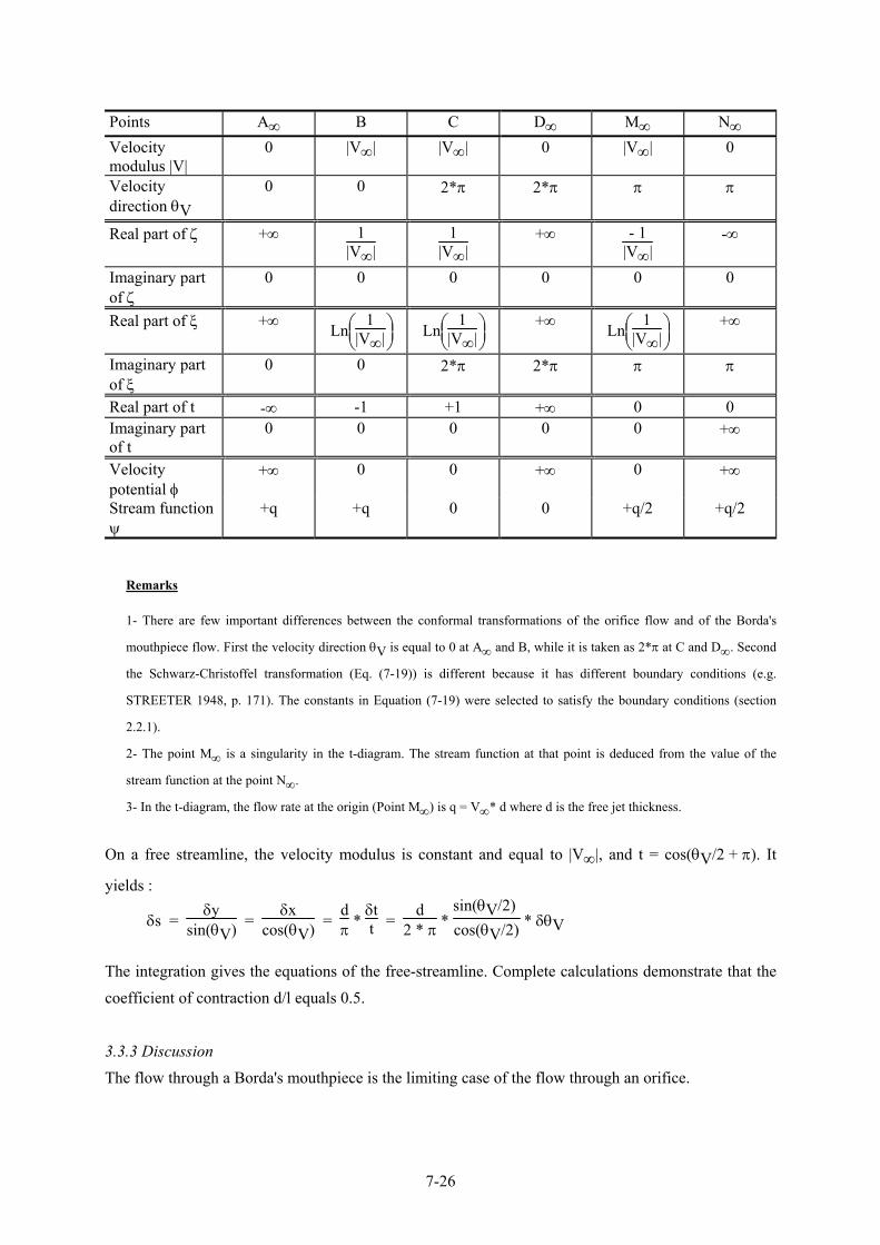
Points A∞ B C D∞ M∞ N∞ Velocity modulus |V|

0 |V∞| |V∞| 0 |V∞| 0

Velocity direction θV

0 0 2*π 2*π π π

Real part of ζ +∞ 1|V∞|

1|V∞|

+∞ - 1|V∞|

-∞

Imaginary part of ζ

0 0 0 0 0 0

Real part of ξ +∞ Ln

1

|V∞| Ln

1

|V∞| +∞ Ln

1

|V∞| +∞

Imaginary part of ξ

0 0 2*π 2*π π π

Real part of t -∞ -1 +1 +∞ 0 0 Imaginary part of t

0 0 0 0 0 +∞

Velocity potential φ

+∞ 0 0 +∞ 0 +∞

Stream function ψ

+q +q 0 0 +q/2 +q/2

Remarks

1- There are few important differences between the conformal transformations of the orifice flow and of the Borda's

mouthpiece flow. First the velocity direction θV is equal to 0 at A∞ and B, while it is taken as 2*π at C and D∞. Second

the Schwarz-Christoffel transformation (Eq. (7-19)) is different because it has different boundary conditions (e.g.

STREETER 1948, p. 171). The constants in Equation (7-19) were selected to satisfy the boundary conditions (section

2.2.1).

2- The point M∞ is a singularity in the t-diagram. The stream function at that point is deduced from the value of the

stream function at the point N∞.

3- In the t-diagram, the flow rate at the origin (Point M∞) is q = V∞* d where d is the free jet thickness.

On a free streamline, the velocity modulus is constant and equal to |V∞|, and t = cos(θV/2 + π). It

yields :

δs = δy

sin(θV) = δx

cos(θV) = dπ *

δtt =

d2 * π *

sin(θV/2) cos(θV/2) * δθV

The integration gives the equations of the free-streamline. Complete calculations demonstrate that the coefficient of contraction d/l equals 0.5.

3.3.3 Discussion The flow through a Borda's mouthpiece is the limiting case of the flow through an orifice.

7-27

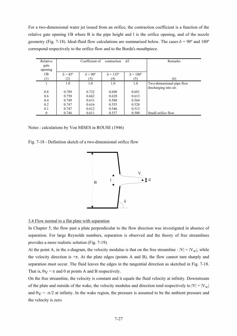
For a two-dimensional water jet issued from an orifice, the contraction coefficient is a function of the relative gate opening l/B where B is the pipe height and l is the orifice opening, and of the nozzle geometry (Fig. 7-18). Ideal-fluid flow calculations are summarised below. The cases δ = 90º and 180º correspond respectively to the orifice flow and to the Borda's mouthpiece.

Relative gate

opening

Coefficient of contraction d/l Remarks

l/B δ = 45º δ = 90º δ = 135º δ = 180º (1) (2) (3) (4) (5) (6) 1 1.0 1.0 1.0 1.0 Two-dimensional pipe flow

discharging into air. 0.8 0.789 0.722 0.698 0.691 0.6 0.758 0.662 0.620 0.613 0.4 0.749 0.631 0.580 0.564 0.2 0.747 0.616 0.555 0.528 0.1 0.747 0.612 0.546 0.513 0 0.746 0.611 0.537 0.500 Small orifice flow.

Notes : calculations by Von MISES in ROUSE (1946) Fig. 7-18 - Definition sketch of a two-dimensional orifice flow

l

δ

Bd

Vo o

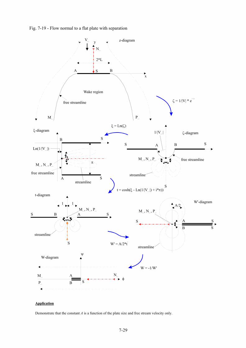
3.4 Flow normal to a flat plate with separation In Chapter 5, the flow past a plate perpendicular to the flow direction was investigated in absence of separation. For large Reynolds numbers, separation is observed and the theory of free streamlines provides a more realistic solution (Fig. 7-19). At the point A, in the z-diagram, the velocity modulus is that on the free streamline : |V| = |V∞|, while the velocity direction is +π. At the plate edges (points A and B), the flow cannot turn sharply and separation must occur. The fluid leaves the edges in the tangential direction as sketched in Fig. 7-18. That is, θV = π and 0 at points A and B respectively. On the free streamline, the velocity is constant and it equals the fluid velocity at infinity. Downstream of the plate and outside of the wake, the velocity modulus and direction tend respectively to |V| = |V∞| and θV = -π/2 at infinity. In the wake region, the pressure is assumed to be the ambient pressure and the velocity is zero.

7-28

Note the stagnation point S on the upstream face of the plate and the two separation points A and B. On the streamline through the stagnation point S, the stream function is taken as ψ = 0. It can be shown that the velocity potential equals zero at stagnation. The basic transformations are :

ζ = - dz

dW = 1

|V| * ei*θV (7-21)

ξ = Ln(ζ) = Ln

1

|V| + i * θV (7-22)

t = cosh

1

2 *

ξ - Ln

1

|V∞| + i * π (7-23)

W' = A * t22 (7-24)

W = - 1

W' (7-25)

The flow pattern is sketched in Figure 7-19. There is one more transformation than in the previous applications. The transformation from the t-diagram to the W'-diagram (Eq. (7-24)) is a Schwarz-Christoffel transformation for a semi-infinite strip of zero thickness (section 2.2.1). In the t-diagram, the real constants a, b and c are arbitrarily selected such that : a = -∞, b = 0, c = +∞, and the external angles of the polygon are β = -π and γ = 0. The Schwarz-Christoffel transformation is :

W' = A * ⌡⌠ dt

t-1 + B (7-24a)

which gives :

W' = A * t22

assuming B = 0 for t = 0 : i.e., at the points N∞, M∞ and P∞. It can be demonstrated that W' must be real along the plate (-1 < t < +1) and that A must be a real positive constant (STREETER 1948 p. 178, VALLENTINE 1969 p. 224). The constant A is a function of the dimensions of the plate :

A = 4 + π

L * |V∞| (7-26)

where L is the half-breadth of the plate (Fig. 7-19).

7-29

Fig. 7-19 - Flow normal to a flat plate with separation

A

free streamline

Wake region

Mo o

Po o

Vo o

No o

BS

z-diagramy

x

2*L

ζ = 1/|V| * ei * Vθ

streamline

free streamline

S

M , N , Po o o o o o

S

S

BA

ζ-diagram1/|V |o o

ξ ζ= Ln( )

streamline

ξ-diagram

free streamline

S

S

M , N , Po o o o o o

B

A

Ln(1/|V |)o o

π

t = cosh( - Ln(1/|V |) + i* ))ξ πo o

W' = A/2*t2

S

S

M , N , Po o o o o o

SB

streamline

A

t-diagram

1 1

S S

S

M , Po o o o o o, N

B

streamline

A

W'-diagramA/2

W = -1/W'

W-diagramψ

φA

B S

No oM

o o

Po o

Application

Demonstrate that the constant A is a function of the plate size and free stream velocity only.

7-30

Solution

On the plate, let consider the streamline ψ = 0 between the stagnation point S and the plate edge A. At stagnation(point

S), the velocity modulus and direction are 0 and +π respectively, while |V| = |V∞| and θV = +π at the plate edge (point

A). Between the points S and A, the velocity vector is : V = |V|*ei*π. That is, t is real and varies from +∞ down to +1 :

t = cosh

Ln

|V∞|

|V| along streamline S-A

It gives :

t = 12 *

exp

Ln

|V∞|

|V| + exp

- Ln

|V∞|

|V| = 12 *

|V∞||V| +

1|V∞||V|

along streamline S-A

and hence :

|V∞||V| = t + t2 - 1 along streamline S-A

which satisfies |V| = 0 at the stagnation point S (t = +∞).

By definition of the velocity potential (Chapters 2 and 3) :

δφδs = -|V| = -

δφδx along streamline S-A

since δx = - δs along the streamline S-A.

On the streamline S-A, the stream function is zero and the complex potential satisfies W = φ :

W = φ = - 1

W' = - 2A *

1

t2 along streamline S-A

Integrating dx in the z-diagram between S and A :

⌡⌠S

Adx = - L = ⌡

⌠

t=+∞

t=+1dxdφ *

dφdt * dt along streamline S-A

where L is the half-breadth of the plate (Fig. 7-19). Since δx/δφ = 1/|V| and

dφdt =

4

A * t3

the integration between S and A gives :

⌡⌠S

Adx = - L =

4A * |V∞| *

⌡⌠

t=+∞

t=+1

t + t2 - 1

t3 * dt along streamline S-A

The right-handside integral term may be integrated analytically (e.g. SPIEGEL 1968). The exact solution yields :

A = 4 + π

L * |V∞|

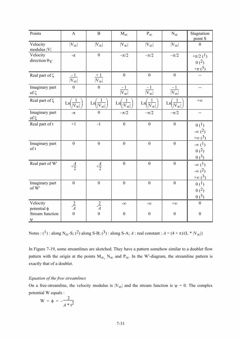
The basic transformations are summarised below for the characteristic points A,B, S, N∞, M∞ and P∞ and sketched in Figure 7-19. Note the singularity of the stagnation point.

7-31

Points A B M∞ P∞ N∞ Stagnation

point S Velocity modulus |V|

|V∞| |V∞| |V∞| |V∞| |V∞| 0

Velocity direction θV

-π 0 −π/2 −π/2 −π/2 +π/2 (1) 0 (2)

+π (3) Real part of ζ - 1

|V∞| + 1

|V∞| 0 0 0 --

Imaginary part of ζ

0 0 - 1|V∞|

- 1|V∞|

- 1|V∞|

--

Real part of ξ Ln

1

|V∞| Ln

1

|V∞| Ln

1

|V∞| Ln

1

|V∞| Ln

1

|V∞| +∞

Imaginary part of ξ

-π 0 −π/2 −π/2 −π/2 --

Real part of t +1 -1 0 0 0 0 (1) -∞ (2) +∞ (3)

Imaginary part of t

0 0 0 0 0 -∞ (1) 0 (2) 0 (3)

Real part of W' +

A2 +

A2

0 0 0 -∞ (1) -∞ (2) +∞ (3)

Imaginary part of W'

0 0 0 0 0 0 (1) 0 (2) 0 (3)

Velocity potential φ -

2A -

2A -∞ -∞ +∞ 0

Stream function ψ

0 0 0 0 0 0

Notes : (1) : along N∞-S; (2) along S-B; (3) : along S-A; A : real constant : A = (4 + π)/(L * |V∞|)

In Figure 7-19, some streamlines are sketched. They have a pattern somehow similar to a doublet flow pattern with the origin at the points M∞, N∞ and P∞. In the W'-diagram, the streamline pattern is exactly that of a doublet.

Equation of the free streamlines On a free-streamline, the velocity modulus is |V∞| and the stream function is ψ = 0. The complex potential W equals :

W = φ = - 2

A * t2

7-32

where t = - cos(θV) and A is a real constant (Eq. (7-26)). The definition of the velocity potential gives:

|V∞| = - δφδs

and φ = - |V∞| * s

where s is measured along the free streamline (ψ = 0) with s = 0 at the plate edge. It yields :

δs = 4

A * |V∞| * sin(θV)

cos3(θV) * δθV

Integrating and replacing A by its expression :

s = 4 * L4 + π *

1cos2(θV)

where θV varied between 0 and -π/2 along the free streamline B-P∞ and between -π and -π/2 along the free streamline A-M∞. By definition, the streamwise coordinate s is tangent to the velocity vector at every point and it satisfies :

δs = δy

sin(θV) = δx

cos(θV)

Hence :

δx = 4

A * |V∞| * sin(θV)

cos2(θV) * δθV

δy = 4

A * |V∞| * sin2(θV)

cos3(θV) * δθV

On the free-streamline B-P∞, the integrations yield :

x = 4 * L4 + π *

π

4 + 1

cos(θV) free streamline B-P∞

y = 2 * L4 + π *

tan(θV) - Ln

tan

θV

2 + π4 free streamline B-P∞

assuming the z-diagram origin at the stagnation point (Fig. 7-19). These parametric equations in terms of θV describe the free streamline B-P∞ for θV varying between 0 and -π/2. A similar development may be conducted for the streamline A-M∞ :

x = - 4 * L4 + π *

π

4 - 1

cos(θV) free streamline A-M∞

y = 2 * L4 + π *

tan(θV) + Ln

- tan

θV

2 + π4 free streamline A-M∞

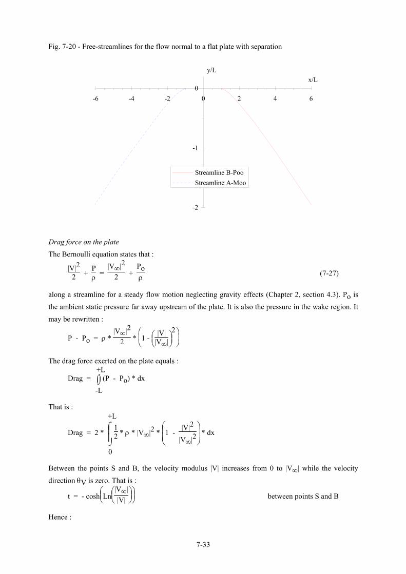
The free streamlines A-M∞ and B-P∞ define the wake region. They are plotted in Figure 7-20 for the flow pattern defined in Figure 7-19.

7-33

Fig. 7-20 - Free-streamlines for the flow normal to a flat plate with separation

-2

-1

0-6 -4 -2 0 2 4 6

Streamline B-PooStreamline A-Moo

y/Lx/L

Drag force on the plate The Bernoulli equation states that :

|V|2

2 + Pρ =

|V∞|2

2 + Poρ (7-27)

along a streamline for a steady flow motion neglecting gravity effects (Chapter 2, section 4.3). Po is the ambient static pressure far away upstream of the plate. It is also the pressure in the wake region. It may be rewritten :

P - Po = ρ * |V∞|2

2 *

1 -

|V|

|V∞|2

The drag force exerted on the plate equals :

Drag = ⌡⌠-L

+L(P - Po) * dx

That is :

Drag = 2 * ⌡⌠

0

+L12 * ρ * |V∞|2 *

1 -

|V|2

|V∞|2 * dx

Between the points S and B, the velocity modulus |V| increases from 0 to |V∞| while the velocity direction θV is zero. That is :

t = - cosh

Ln

|V∞|

|V| between points S and B

Hence :

7-34

- t = 12 *

|V∞|

|V| + |V|

|V∞|

It can be shown that :

- 2 * t2 - 1 =

|V∞|

|V| - |V|

|V∞|

Between S and B, the stream function y equals zero and the complex potential satisfies :

δW = δφ = - |V| * δx = - 4

Α * t3 * δt

Replacing into the expression of the drag force, it yields :

Drag = - 8 * ρ * |V∞|

A * ⌡⌠

-∞

-1

t2 - 1t3

* dt

where A = (4 + π)/(L * |V∞|). It may be rewitten :

Drag = CD * (2 * L) * ρ * V∞

2

2 (7-28)

where the drag coefficient CD equals :

CD = 2 * π

π + 4 = 0.8798 (7-29)

Remark

1- The integration of the drag force has an exact solution since :

⌡⌠

-∞

-1

t2 - 1

t3 * dt = -

t2 - 1

2 * t2 +

12 * cos-1

1|t|

Discussion The above analysis for an ideal fluid flow assuming that the wake is at rest and the pressure in the wake region equals the pressure Po in the undisturbed stream. This approximation may apply when a stream of water flows past a flat plate and that the space between the separation lines is filled with air (7). If the wake is filled with a fluid of density comparable to the main stream, flow recirculation develops behind the plate and the pressure behind the plate is less than that of the undisturbed stream, yielding greater drag on the plate. Considering a real fluid flow past a two-dimensional plate, experiments show that the drag coefficient is CD = 1.90 for Re > 1 E+3, where the drag coefficient is defined as :

7or water vapour in the case of high-velocity flows and cavitating flows.

7-35

Drag = CD * A * ρ * V∞

2

2

where A is the projected area of the body. The result is valid for two dimensional flows. Note that it is more than twice the calculated drag coefficient (Eq. (7-29)). Plates of finite widths have a lower drag because three-dimensional flows occur at the ends. For a plate of length 2*L (Fig. 7-9) and of width B (8), the measured drag coefficient is :

B/(2*L) CD Re Remarks (1) (2) (3) (4) +∞ 1.90 > 1E+3 Two-dimensional flows 20 1.50 5 1.20 1 1.16

For a circular disk, the observed drag coefficient is about CD = 1.12 for Re > 1 E+3.

Remarks

1- For the flow past a blunt body (e.g. flat plate), the drag coefficient is defined using the projected area. For example, A

= π*R2 for a circular cylinder of radius R. But, in the study of flows past airfoils, the area A is defined as the chord times

the width of the foil (Chapter 6).

2- Experimental results showed that the drag coefficient is basically independent of the the Reynolds number for Re > 1

E+3.

4. Summary

The theory of free streamlines associated with the theorem of Schwarz-Christoffel is a power technique to solve analytically ideal fluid flow with separation. Basic applications include the flow through an orifice and the flow past a normal plate. However it must be emphasised that it is a difficult technique involving several successive transformations. In the wake region, the velocity is assumed zero. While the approximation may be suitable when the wake contains a fluid of lesser density than the main stream, it yields often lower drag force estimates. Further gravity effects were ignored in the above developments.

8in the direction normal to the x-y plane.