chapter 7 transportation problems ( 運輸問題 ) assignment problems ( 指派問題 )...
TRANSCRIPT

Chapter 7
Transportation Problems ( 運輸問題 )
Assignment Problems ( 指派問題 )
Transshipment Problems ( 轉運問題 )

2
簡介 Transportation Problems ( 運輸問題 )
如何以最低之運輸成本,將貨物由來源地送至目的地 Assignment Problems ( 指派問題 )
如何以適當之方式,做一對一之指派為運輸問題之特例
Transshipment Problems ( 轉運問題 )在運輸問題中,允許貨物由來源地經由其他來源地或目的地轉運,最後送至目的地
上述之線性規劃模式仍然可以單體法求解,但有特別之求解方式,遠較單體法來得有效率。

3
7.1 Transportation Problems
A transportation problem( 運輸問題 ) deals with the problem, which aims to find the best way to fulfill the demand of n demand points( 需求點 ) using the capacities of m supply points ( 供應點 ).
While trying to find the best way, generally a variable cost of shipping the product from one supply point to a demand point or a similar constraint should be taken into consideration.
p.360
4
Example 1: Powerco Formulation
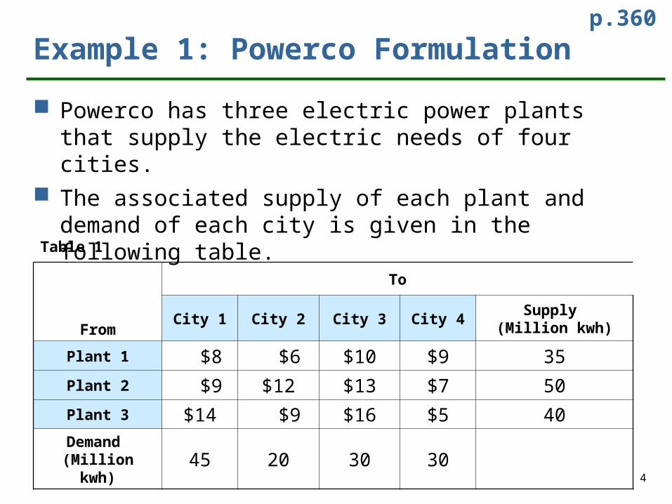
Powerco has three electric power plants that supply the electric needs of four cities.
The associated supply of each plant and demand of each city is given in the following table.
p.360
Table 1
From
To
City 1 City 2 City 3 City 4Supply
(Million kwh)
Plant 1 $8 $6 $10 $9 35
Plant 2 $9 $12 $13 $7 50
Plant 3 $14 $9 $16 $5 40Demand
(Million kwh) 45 20 30 30
5
Example 1: Solution
Decision VariablesPowerco must determine how much power is sent from each plant to each city so xij = amount of electricity produced at plant i and sent to city j
ConstraintsA supply constraint( 供應限制 )ensures that the
total quality produced does not exceed plant capacity. Each plant is a supply point.
A demand constraint ( 需求限制 ) ensures that a location receives its demand. Each city is a demand point.
Since a negative amount of electricity can not be shipped all xij’s must be non negative
6
From
To
City 1 City 2 City 3 City 4 Supply (Million kwh)
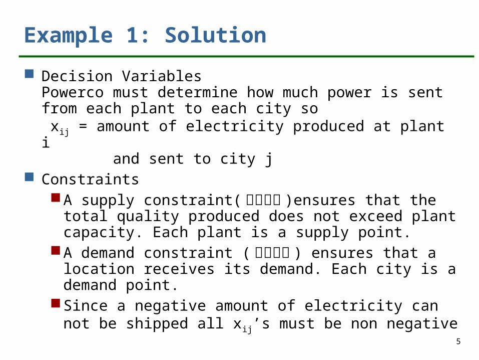
Plant 1 8x11 6x12 10x13 9x14 ≤ 35
Plant 2 9x21 12x22 13x23 7x24 ≤ 50
Plant 3 14x31 9x32 16x33 5x34 ≤ 40
Demand (Million kwh)
≥ 45 ≥ 20 ≥ 30 ≥ 30
Min z = 8x11+6x12+10x13+9x14+9x21+12x22+13x23
+7x24 +14x31+9x32+16x33+5x34
s.t. x11+x12+x13+x14 ≤ 35 (Supply Constraints)
x21+x22+x23+x24 ≤ 50
x31+x32+x33+x34 ≤ 40
x11+x21+x31 ≥ 45 (Demand Constraints)
x12+x22+x32 ≥ 20
x13+x23+x33 ≥ 30
x14+x24+x34 ≥ 30
xij ≥ 0 (i= 1,2,3; j= 1,2,3,4)

7
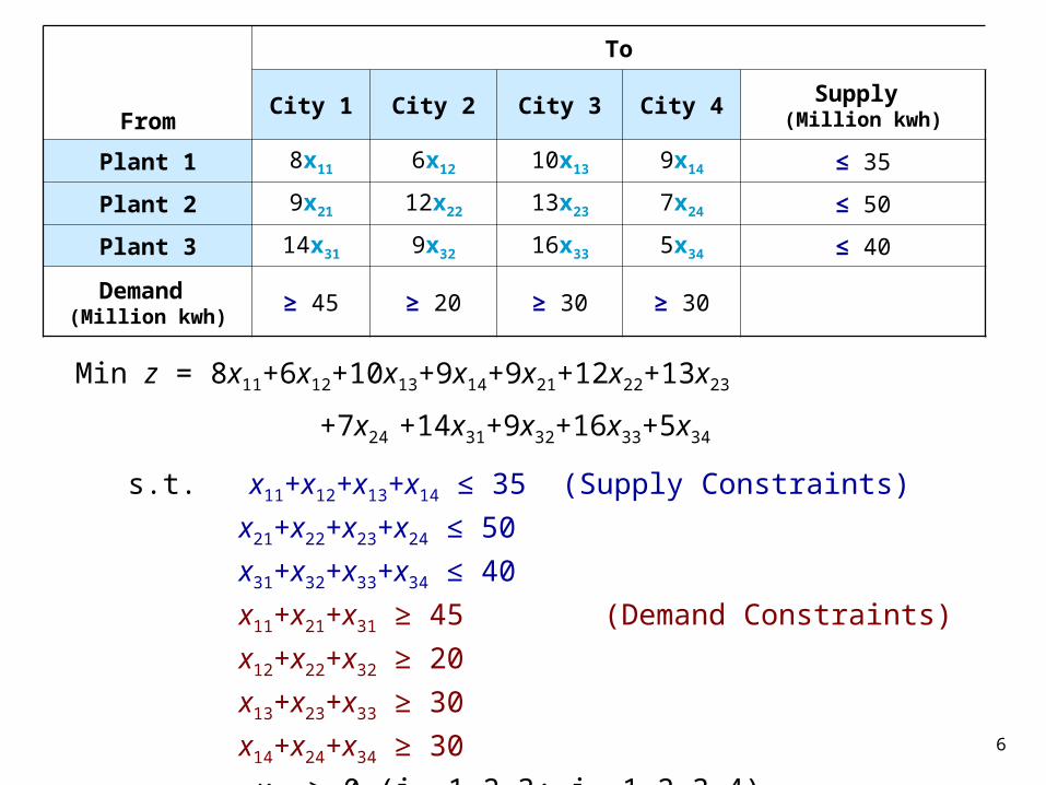
General description of a Transportation Problem
A set of m supply points from which a good is shipped. Supply point i can supply at most si units.
A set of n demand points to which the good is shipped. Demand point j must receive at least di units of the shipped good.
Each unit produced at supply point i and shipped to demand point j incurs a variable cost of cij.
Table 2 (p.364).
p.362
8
Table 2 Supply
C11 C12…
C1n S1
C21 C22…
C2n S2
: : :
Cm1 Cm2…
Cmn Sm
Demand D1 D2 … Dn
p.364A Transportation Tableau
9
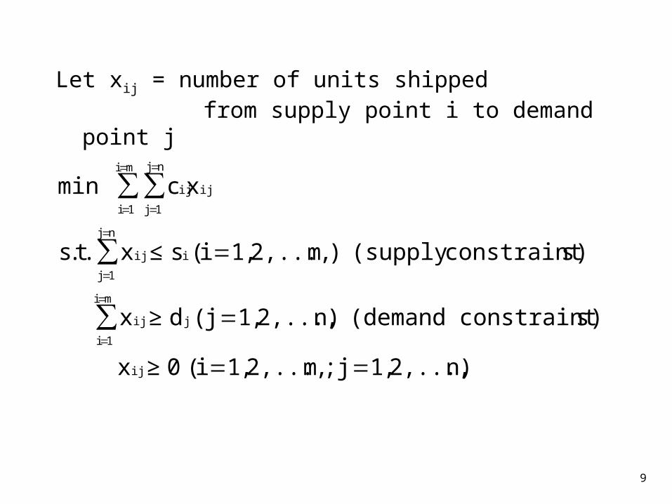
Let xij = number of units shipped
from supply point i to demand point j
)n,...,2,1j;m,...,2,1i( 0x
s)constraint (demand )n,...,2,1j( dx
s)constraint (supply )m,...,2,1i( sx .t.s
xc min
ij
mi
1i
jij
nj
1j
iij
mi
1i
nj
1j
ijij
≥
≥
≤
∑
∑
∑∑

10
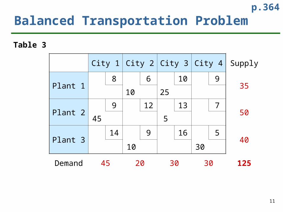
Balanced Transportation Problem
If
then total supply equals to total demand,the problem is said to be a balanced transportation problem ( 平衡運輸問題 ).
nj
1j
j
mi
1i
i ds
p.363
11
Balanced Transportation Problem
Table 3
City 1 City 2 City 3 City 4 Supply
Plant 18 6 10 9
3510 25
Plant 29 12 13 7
5045 5
Plant 314 9 16 5
4010 30
Demand 45 20 30 30 125
p.364

12
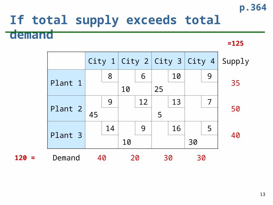
If total supply exceeds total demand
If
total supply exceeds total demand, we can balance the problem by adding dummy demand point ( 虛擬需求點 ). Since shipments to the dummy demand point are not real, they are assigned a cost of zero.
Figure 2 (p.364).
∑∑n=j
1=jj
m=i
1=ii d> s
13
If total supply exceeds total demand
=125
City 1 City 2 City 3 City 4 Supply
Plant 18 6 10 9
3510 25
Plant 29 12 13 7
5045 5
Plant 314 9 16 5
4010 30
120 = Demand 40 20 30 30
p.364
14
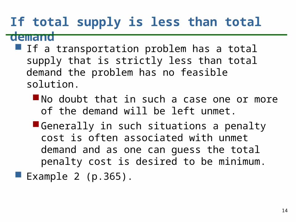
If total supply is less than total demand If a transportation problem has a total supply that
is strictly less than total demand the problem has no feasible solution. No doubt that in such a case one or more of the
demand will be left unmet. Generally in such situations a penalty cost is
often associated with unmet demand and as one can guess the total penalty cost is desired to be minimum.
Example 2 (p.365).

15
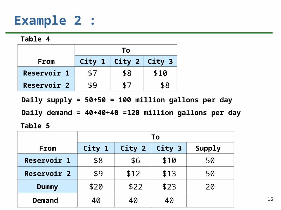
Example 2 : Handing Shortages
Two reservoirs are available to supply the water needs of three cities. Each reservoir can supply up to 50 million gallons of water per day. Each city would like to receive 40 million gallons per day. For each million gallons per day of unmet demand, there is a penalty. At city 1, the penalty is $20; at city 2, the penalty is $22; and at city 3, the penalty is $23. The cost of transporting 1 million gallons of water from each reservoir to each city is shown in Table 4. Formulate a balanced transportation problem that can be used to minimize the sum of shortage and transport costs.
p.365
16
Example 2 :Table 4
From
To
City 1 City 2 City 3
Reservoir 1 $7 $8 $10
Reservoir 2 $9 $7 $8
Daily supply = 50+50 = 100 million gallons per day
Daily demand = 40+40+40 =120 million gallons per day
Table 5
From
To
City 1 City 2 City 3 Supply
Reservoir 1 $8 $6 $10 50
Reservoir 2 $9 $12 $13 50
Dummy $20 $22 $23 20
Demand 40 40 40

17
Exercise 1 :p.371
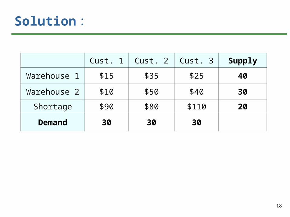
A company supplies goods to three customers, who each require 30 units. The company has two warehouses. Warehouses 1 has 40 units available, and warehouses 2 has 30 units available. The cost of shipping 1 unit from warehouse to customer are shown in Table 7. There is penalty for each unmet customer unit of demand: With customer 1, a penalty cost of $90 incurred; with customer 2, $80; and with customer 3, $110. Formulate a balanced transportation problem to minimize the sum of shortage and shipping costs.
Table 7
Cust. 1 Cust. 2 Cust. 3
Warehouse 1 $15 $35 $25
Warehouse 2 $10 $50 $40
18
Solution :
Cust. 1 Cust. 2 Cust. 3 Supply
Warehouse 1 $15 $35 $25 40
Warehouse 2 $10 $50 $40 30
Shortage $90 $80 $110 20
Demand 30 30 30

19
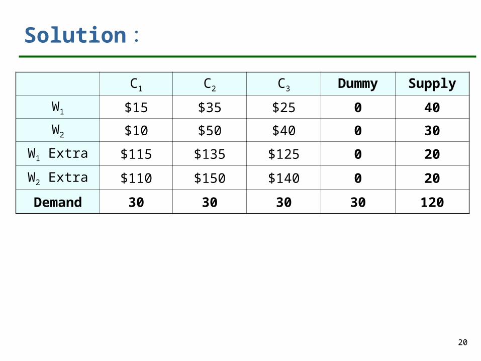
Exercise 2 :
Referring to exercise 1, suppose that extra units could be purchases and shipped to either warehouse for a total cost of $100 per unit and that all customer demand must be met. Formulate a balanced transportation problem to minimize the sum of purchasing and shipping costs.
20
Solution :
C1 C2 C3 Dummy Supply
W1 $15 $35 $25 0 40
W2 $10 $50 $40 0 30
W1 Extra $115 $135 $125 0 20
W2 Extra $110 $150 $140 0 20
Demand 30 30 30 30 120
21
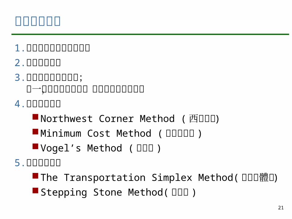
運輸問題求解
1.將問題建成運輸問題模式2.平衡運輸問題3.求解過程分為二階段;
第一階段為求起始解,第二階段為求最佳解4.起始解之解法
Northwest Corner Method ( 西北角法 )Minimum Cost Method ( 最小成本法 )Vogel’s Method ( 佛格法 )
5.最佳解之解法The Transportation Simplex Method( 運輸單體法 )Stepping Stone Method( 階石法 )
22
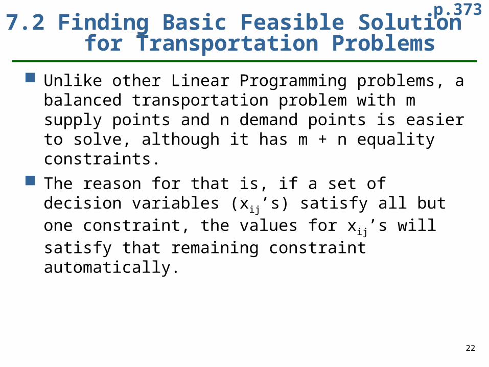
7.2 Finding Basic Feasible Solution for Transportation Problems
Unlike other Linear Programming problems, a balanced transportation problem with m supply points and n demand points is easier to solve, although it has m + n equality constraints.
The reason for that is, if a set of decision variables (xij’s) satisfy all but one constraint, the values for xij’s will satisfy that remaining constraint automatically.
p.373
23
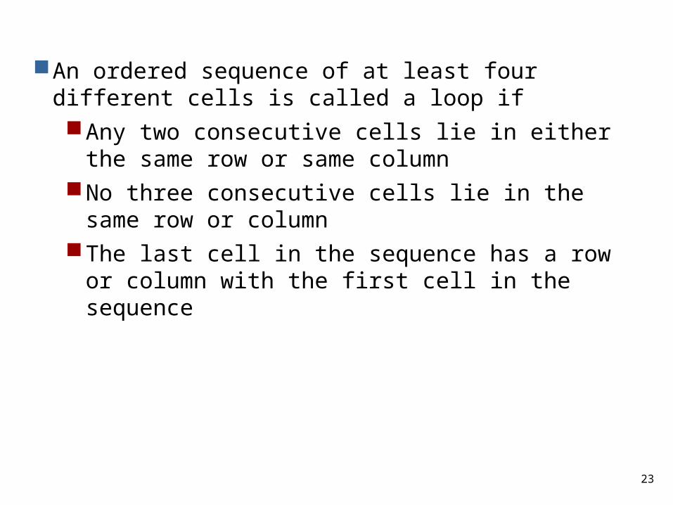
An ordered sequence of at least four different cells
is called a loop if Any two consecutive cells lie in either the same
row or same columnNo three consecutive cells lie in the same row or
columnThe last cell in the sequence has a row or
column with the first cell in the sequence

24
The Northwest Corner Method dos not utilize
shipping costs. It can yield an initial bfs easily but the total shipping cost may be very high.
The Minimum Cost Method uses shipping costs in order come up with a bfs that has a lower cost. Often the minimum cost method will yield a costly bfs.
Vogel’s Method for finding a bfs usually avoids extremely high shipping costs.

25
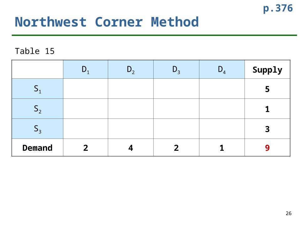
Northwest Corner Method ( 西北角法 )
Begin in the upper left (northwest) corner of the transportation tableau and set x11 as large as possible. x11 can clearly be no larger than the smaller of s1 and d1.
Continue applying this procedure to the most northwest cell in the tableau that does not lie in a crossed-out row or column.
Assign the last cell a value equal to its row or column demand, and cross out both cells row and column.
Table 15 ~ Table 20.
p.376
26
Northwest Corner Method
Table 15
D1 D2 D3 D4 Supply
S1 5
S2 1
S3 3
Demand 2 4 2 1 9
p.376
27
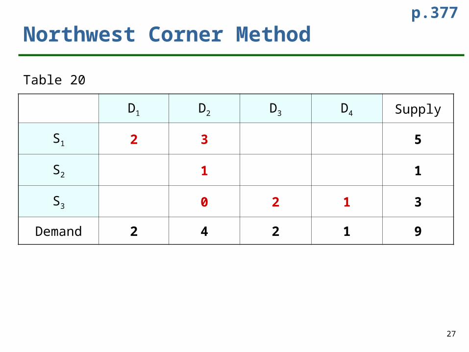
Northwest Corner Method
Table 20
D1 D2 D3 D4 Supply
S1 2 3 5
S2 1 1
S3 0 2 1 3
Demand 2 4 2 1 9
p.377
28
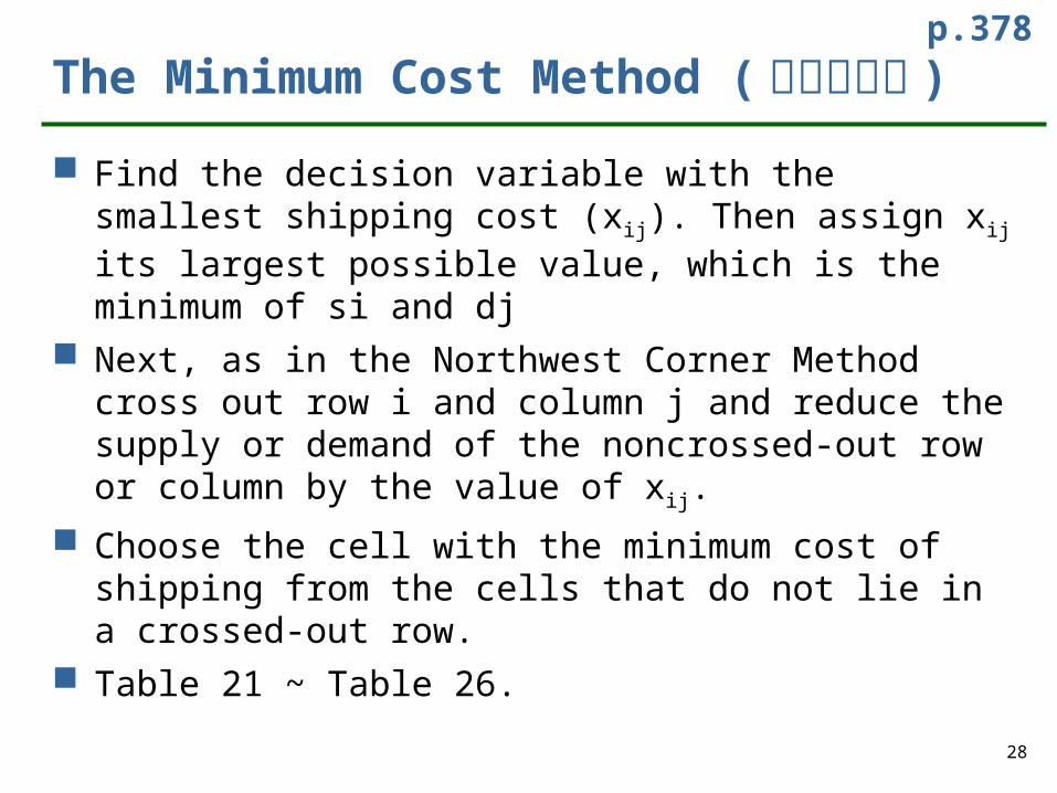
The Minimum Cost Method ( 最小成本法 ) Find the decision variable with the smallest
shipping cost (xij). Then assign xij its largest possible value, which is the minimum of si and dj
Next, as in the Northwest Corner Method cross out row i and column j and reduce the supply or demand of the noncrossed-out row or column by the value of xij.
Choose the cell with the minimum cost of shipping from the cells that do not lie in a crossed-out row.
Table 21 ~ Table 26.
p.378
29
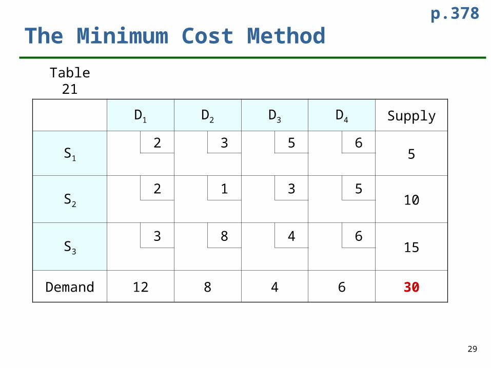
The Minimum Cost Method
Table 21
D1 D2 D3 D4 Supply
S1
2 3 5 65
S2
2 1 3 510
S3
3 8 4 615
Demand 12 8 4 6 30
p.378
30
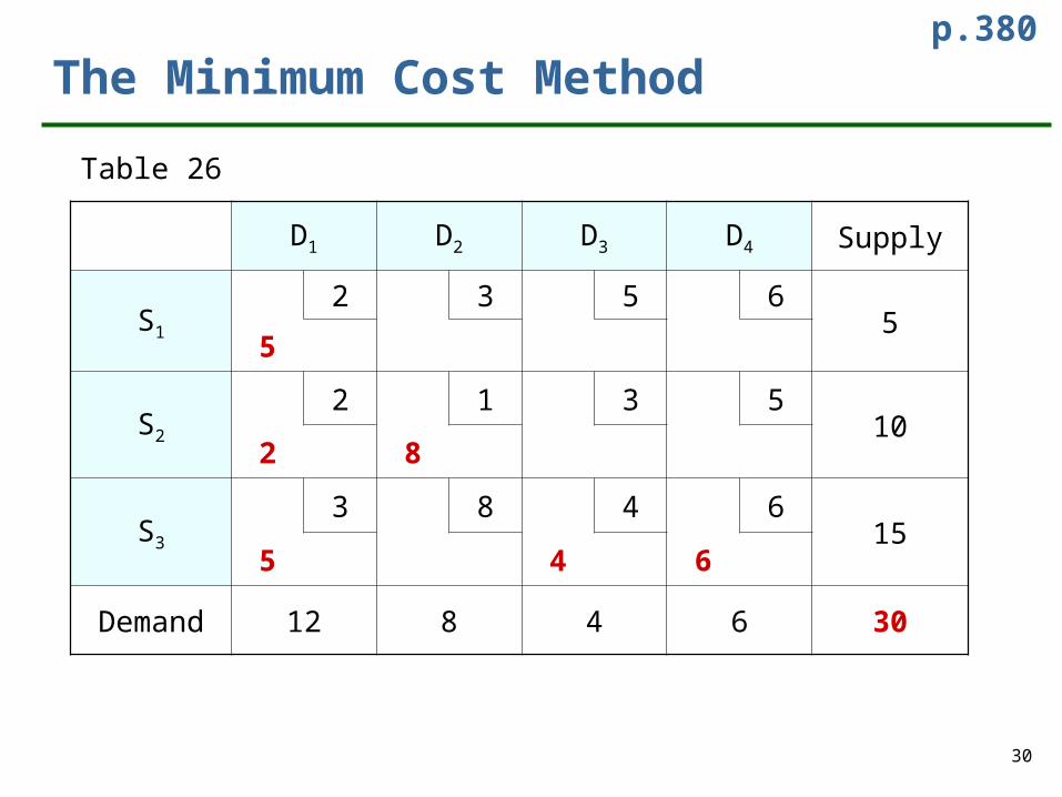
The Minimum Cost Method
Table 26
D1 D2 D3 D4 Supply
S1
2 3 5 65
5
S2
2 1 3 510
2 8
S3
3 8 4 615
5 4 6
Demand 12 8 4 6 30
p.380

31
The Vogel’s Method ( 佛格法 )
Begin with computing each row and column a penalty. The penalty will be equal to the difference between the two smallest shipping costs in the row or column.
Identify the row or column with the largest penalty. Find the first basic variable which has the smallest
shipping cost in that row or column. Assign the highest possible value to that variable,
and cross-out the row or column as in the previous methods.
Compute new penalties and use the same procedure. Table 28 ~ Table 32.
p.380

32
The Vogel’s Method ( 佛格法 )
①計算每列剩餘格中最小與次小之差 (penalty)
②計算每行剩餘格中最小與次小之差 (penalty)
③找出 Max{,}
④找出產生之列或行剩餘格中之最小成本
33
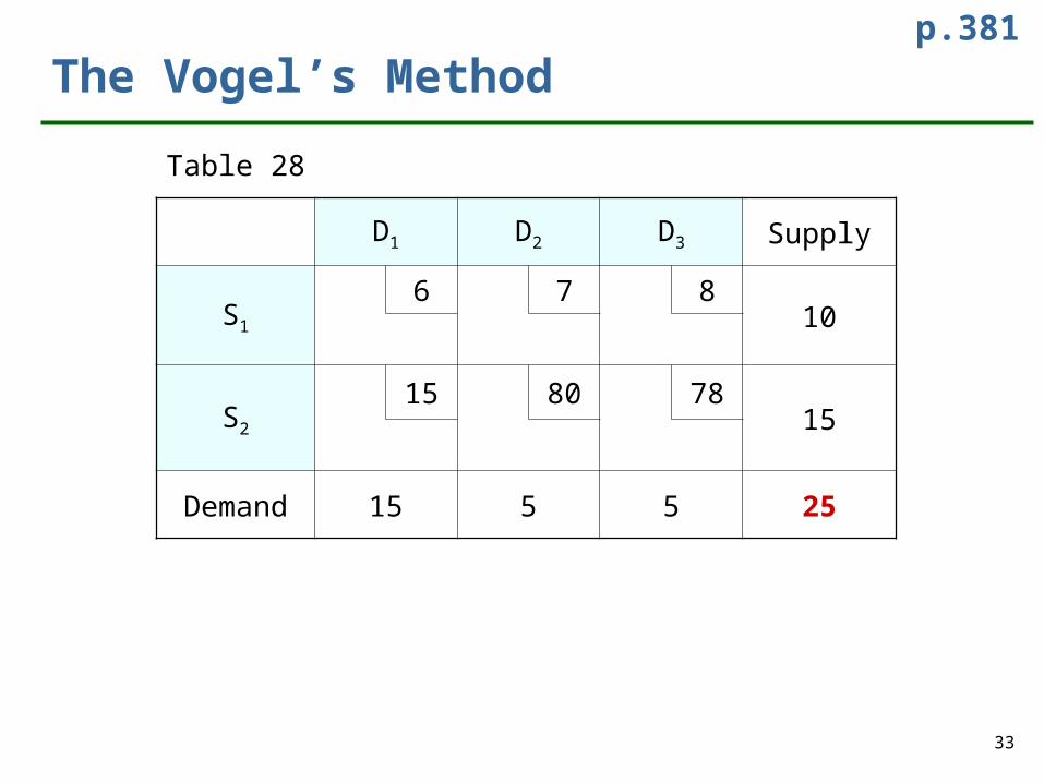
The Vogel’s Method
Table 28
D1 D2 D3 Supply
S1
6 7 810
S2
15 80 7815
Demand 15 5 5 25
p.381
34
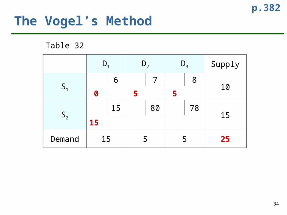
The Vogel’s Method
Table 32
D1 D2 D3 Supply
S1
6 7 810
0 5 5
S2
15 80 7815
15
Demand 15 5 5 25
p.382

35
Exercise 1 :
To find A bfs by the following methods .(1)Northwest Corner Method (2)Minimum Cost Method(3)Vogel’s Method
C1 C2 C3 Supply
W1 $15 $35 $25 40
W2 $10 $50 $40 30
Shortage $90 $80 $110 20
Demand 30 30 30
p.382

36
Solution : Northwest Corner Method
C1 C2 C3 Supply
W1 30 10 40
W2 20 10 30
Shortage 0 20
Demand 30 30 30
37
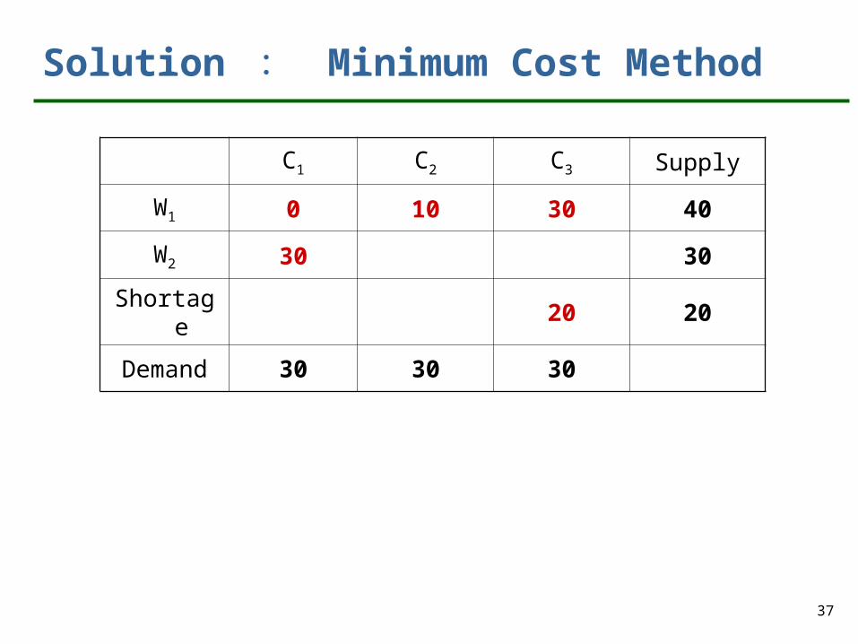
Solution : Minimum Cost Method
C1 C2 C3 Supply
W1 0 10 30 40
W2 30 30
Shortage 20 20
Demand 30 30 30
38
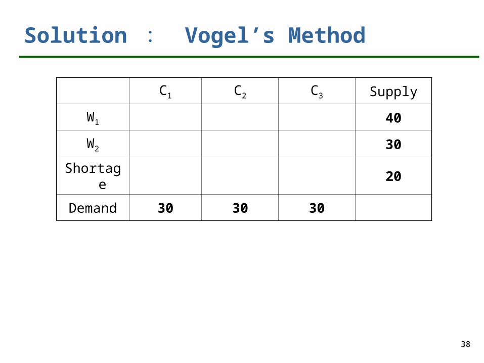
Solution : Vogel’s Method
C1 C2 C3 Supply
W1 40
W2 30
Shortage 20
Demand 30 30 30
39
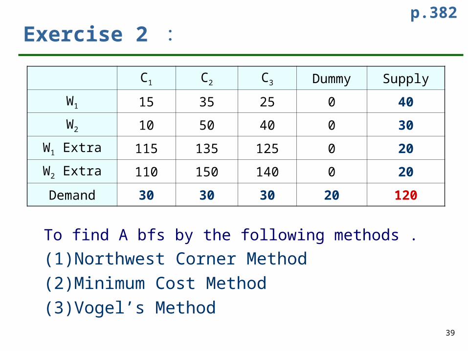
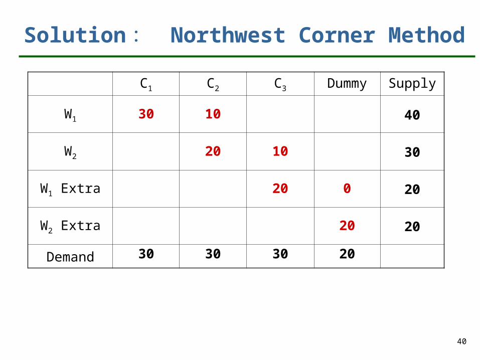
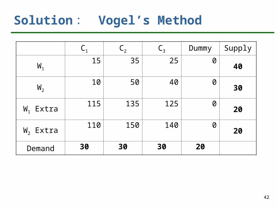
Exercise 2 :
C1 C2 C3 Dummy Supply
W1 15 35 25 0 40
W2 10 50 40 0 30
W1 Extra 115 135 125 0 20
W2 Extra 110 150 140 0 20
Demand 30 30 30 20 120
To find A bfs by the following methods .
(1)Northwest Corner Method (2)Minimum Cost Method(3)Vogel’s Method
p.382
40
Solution : Northwest Corner Method
C1 C2 C3 Dummy Supply
W1 30 10 40
W2 20 10 30
W1 Extra 20 0 20
W2 Extra 20 20
Demand 30 30 30 20

41
Solution : Minimum Cost Method
C1 C2 C3 Dummy Supply
W1
15 35 25 040
W2
10 50 40 030
W1 Extra115 135 125 0
20
W2 Extra110 150 140 0
20
Demand 30 30 30 20
42
Solution : Vogel’s Method
C1 C2 C3 Dummy Supply
W1
15 35 25 040
W2
10 50 40 030
W1 Extra115 135 125 0
20
W2 Extra110 150 140 0
20
Demand 30 30 30 20
43
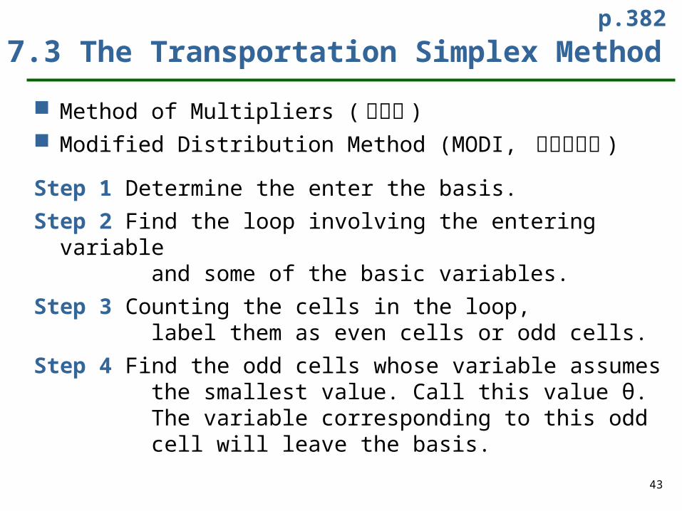
7.3 The Transportation Simplex Method
Method of Multipliers ( 乘數法 ) Modified Distribution Method (MODI, 修正分配法 )
Step 1 Determine the enter the basis.
Step 2 Find the loop involving the entering variable and some of the basic variables.
Step 3 Counting the cells in the loop, label them as even cells or odd cells.
Step 4 Find the odd cells whose variable assumes the smallest value. Call this value θ. The variable corresponding to this odd cell will leave the basis.
p.382

44
To perform the pivot, decrease the value of each odd cell by θ and increase the value of each even cell by θ. The variables that are not in the loop remain unchanged. The pivot is now complete. If θ=0, the entering variable will equal 0, and
an odd variable that has a current value of 0 will leave the basis. In this case a degenerate bfs existed before and will result after the pivot.
If more than one odd cell in the loop equals θ, you may arbitrarily choose one of these odd cells to leave the basis; again a degenerate bfs will result

45
Two important points to keep in mind in the pivoting procedureSince each row has as many +20s as –20s,
the new solution will satisfy each supply and demand constraint.
By choosing the smallest odd variable (x23) to leave the basis, we ensured that all variables will remain nonnegative.

46
單體法求解步驟 ( 複習一下 !!)
1. 建立起始可行解2. 最佳測試 , 決定 entering var.
3. 決定 leaving var.
4. 建立下一個可行解

47
Summary of the Transportation Simplex Method
Step1. Balance problem.
Step2. Find a bfs. (initial solution)
Step3. Let u1=0, cij=ui+vj for all BV. Find ui ,vj.
Step4. Let =ui+vj-cij
If for all NBV, then the current bfs is optimal
else the var with the most positive is a new bfs.
Step5. using the new bfs return to step 3 and 4.
Step4’.
ijc
p.387
0c ≤ij
ijc
0≥c ij
For a min problem
For a max problem
48
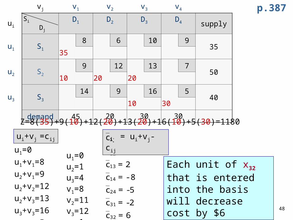
vj v1 v2 v3 v4
uiSi Dj D1 D2 D3 D4 supply
u1 S1
8 6 10 935
35
u2 S2
9 12 13 750
10 20 20
u3 S3
14 9 16 540
10 30
demand 45 20 30 30
u1=0u2=1u3=4v1=8v2=11v3=12v4=1
u1=0
u1+v1=8
u2+v1=9
u2+v2=12
u2+v3=13
u3+v3=16
u3+v4=5
ui+vj =cij
6=c
2-=c
5-=c
-8=c
2=c
5=c
32
31
24
14
13
12
Each unit of x32 that is entered into the basis will decrease cost by $6
Z=8(35)+9(10)+12(20)+13(20)+16(10)+5(30)=1180
p.387
= ui+vj-cijijc
49
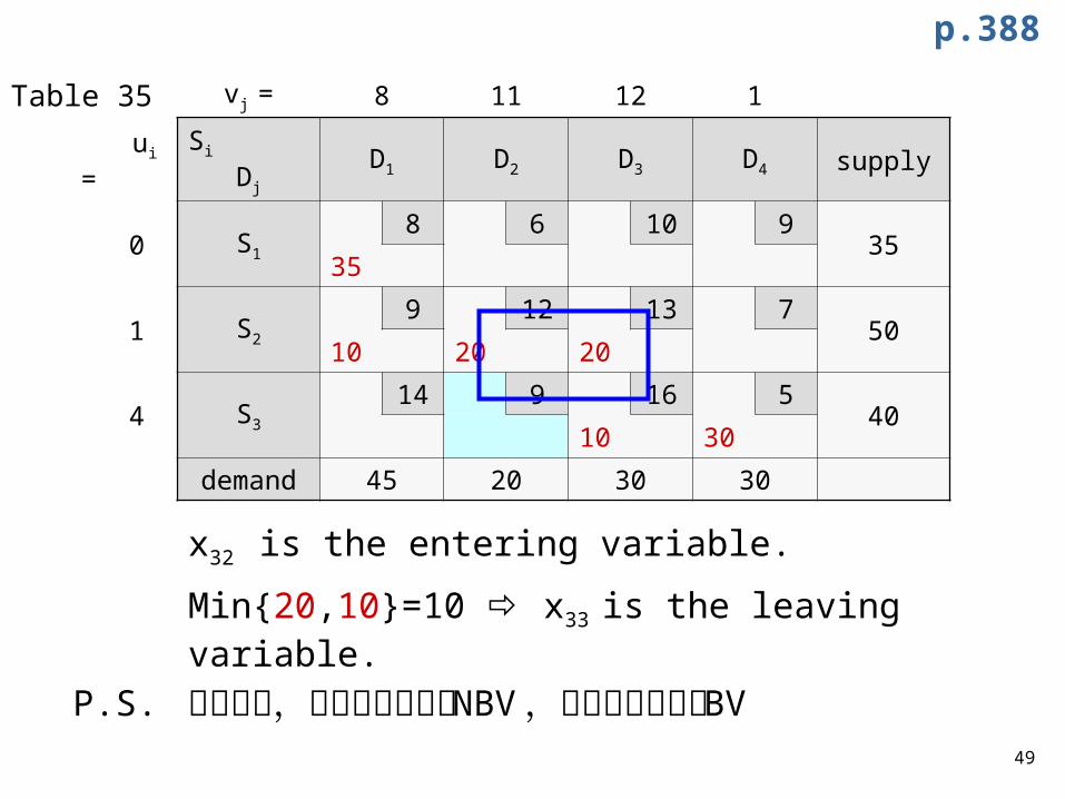
p.388
Table 35 vj = 8 11 12 1
ui = Si Dj D1 D2 D3 D4 supply
0 S1
8 6 10 935
35
1 S2
9 12 13 750
10 20 20
4 S3
14 9 16 540
10 30
demand 45 20 30 30
x32 is the entering variable.
P.S. 閉迴路中,除起點與終點為 NBV ,其餘轉角點均為BV
Min{20,10}=10 x33 is the leaving variable.
50
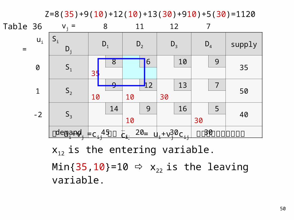
Table 36 vj = 8 11 12 7
ui = Si Dj D1 D2 D3 D4 supply
0 S1
8 6 10 935
35
1 S2
9 12 13 750
10 10 30
-2 S3
14 9 16 540
10 30
demand 45 20 30 30
x12 is the entering variable.
Min{35,10}=10 x22 is the leaving variable.
以 ui+vj =cij 計算 = ui+vj-cij 選擇正最大為進入變數ijc
Z=8(35)+9(10)+12(10)+13(30)+910)+5(30)=1120

51
Table 37 vj = 8 6 12 2
ui = Si Dj D1 D2 D3 D4 supply
0 S1
8 6 10 935
25 10
1 S2
9 12 13 750
20 30
3 S3
14 9 16 540
10 30
demand 45 20 30 30
x13 is the entering variable.
Min{25,30}=25 x11 is the leaving variable.
Z=8(35)+6(10)+9(20)+13(30)+9(10)+5(30)=1050
52
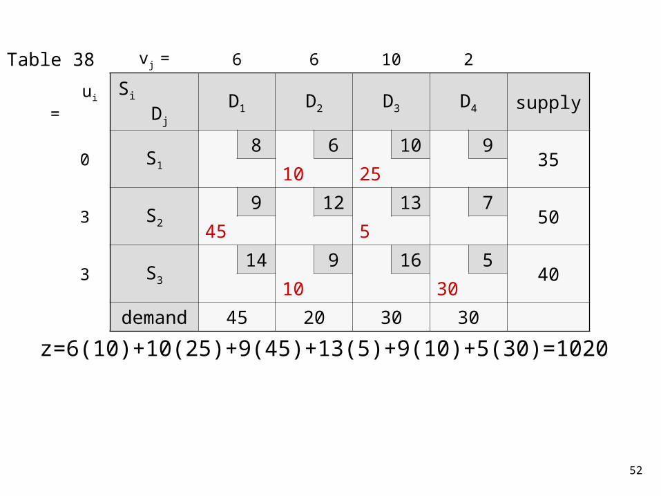
Table 38 vj = 6 6 10 2
ui = Si Dj D1 D2 D3 D4 supply
0 S1
8 6 10 935
10 25
3 S2
9 12 13 750
45 5
3 S3
14 9 16 540
10 30
demand
45 20 30 30
z=6(10)+10(25)+9(45)+13(5)+9(10)+5(30)=1020

53
Exercise : use the transportation simplex method to solve the problem.
vj =
ui =
D1 D2 D3 D4 supply
S1
3 11 3 1017
4 13
S2
1 9 2 824
13 11
S3
7 4 10 519
16 3
demand 13 16 15 16
z=3(4)+10(13)+1(11)+2(11)+4(16)+5(3)=256

54
Exercise : use the transportation simplex method to solve p.382 #1 #2
55
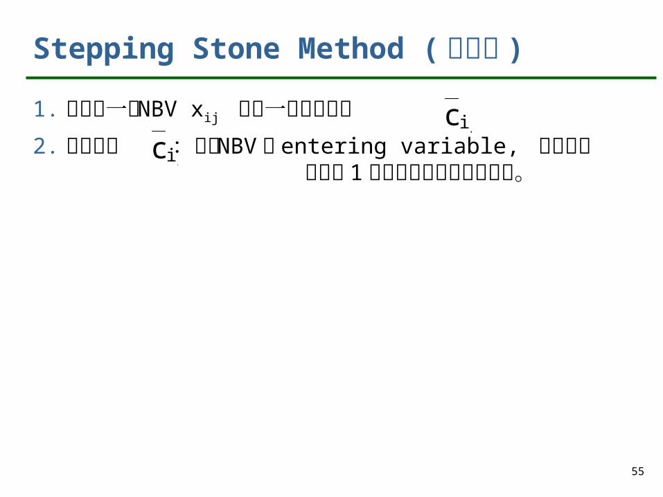
Stepping Stone Method ( 階石法 )
1. 對於每一個 NBV xij 對應一個邊際成本2. 邊際成本 :以該 NBV 為 entering variable, 其運輸
量 每增加 1 單位總運輸成本的增加量。
ijcijc

56
D1 D2 D3 D4 supply
S1
3 11 3 1017
x11 4 13
S2
1 9 2 824
13 11
S3
7 4 10 519
16 3
demand 13 16 15 16
D1 D2 D3 D4 supply
S1
3 11 3 1017
x12 4 13
S2
1 9 2 824
13 11
S3
7 4 10 519
16 3
demand 13 16 15 16
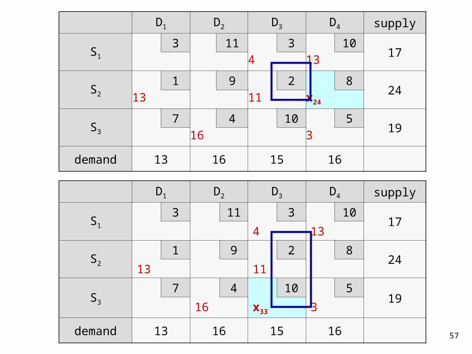
57
D1 D2 D3 D4 supply
S1
3 11 3 1017
4 13
S2
1 9 2 824
13 11 x24
S3
7 4 10 519
16 3
demand 13 16 15 16
D1 D2 D3 D4 supply
S1
3 11 3 1017
4 13
S2
1 9 2 824
13 11
S3
7 4 10 519
16 x33 3
demand 13 16 15 16
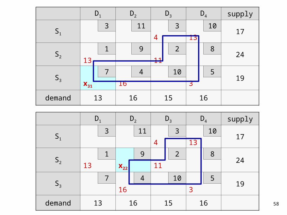
58
D1 D2 D3 D4 supply
S1
3 11 3 1017
4 13
S2
1 9 2 824
13 11
S3
7 4 10 519
x31 16 3
demand 13 16 15 16
D1 D2 D3 D4 supply
S1
3 11 3 1017
4 13
S2
1 9 2 824
13 x22 11
S3
7 4 10 519
16 3
demand 13 16 15 16

59
0>1=C-C+C-C+C-C=C
0>10=C-C+C-C+C-C=C
0>12=C-C+C-C=C
0<1-=C-C+C-C=C
0>2=C-C+C-C=C
0>1=C-C+C-C=C
32341413232222
34141323213131
1314343333
2313142424
2334141212
2123131111
◎ x24 : entering variable
D1 D2 D3 D4 supply
S1
3 11 3 1017
4 13
S2
1 9 2 824
13 11 x24
S3
7 4 10 519
16 3
demand 13 16 15 16
Min{13,11}=11 x23 : leaving variable

60
D1 D2 D3 D4 supply
S1
3 11 3 1017
4+11 13-11
S2
1 9 x23 2 X24 824
13 11-11 0+11
S3
7 4 10 519
16 3
demand 13 16 15 16
x24 : EV
x23 : LV
D1 D2 D3 D4 supply
S1
3 11 3 1017
15 2
S2
1 9 2 824
13 11
S3
7 4 10 519
16 3
demand 13 16 15 16
Z=245<256
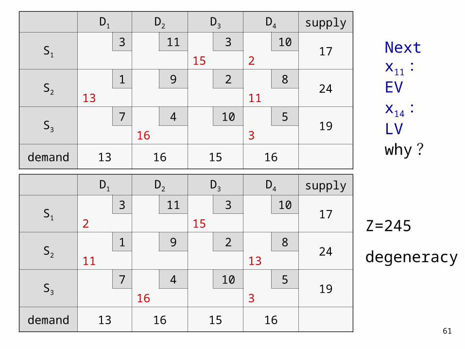
61
Next x11 :EVx14 :LV why ?
D1 D2 D3 D4 supply
S1
3 11 3 1017
15 2
S2
1 9 2 824
13 11
S3
7 4 10 519
16 3
demand 13 16 15 16
D1 D2 D3 D4 supply
S1
3 11 3 1017
2 15
S2
1 9 2 824
11 13
S3
7 4 10 519
16 3
demand 13 16 15 16
Z=245
degeneracy

62
7.5. Assignment Problems
Assignment problems( 指派問題 ) are a certain class of transportation problems for which transportation simplex is often very inefficient.
In general an assignment problem is balanced transportation problem in which all supplies and demands are equal to 1.
The assignment problem’s matrix of costs is its cost matrix( 成本矩陣 ).
All the supplies and demands for this problem are integers which implies that the optimal solution must be integers.
Using the minimum cost method a highly degenerate bfs is obtained.
p.393

63
Example 4: Machine Assignment Problem
Machineco has four jobs to be completed. Each machine must be assigned to complete one job. The time required to setup each machine for
completing each job is shown.
Machineco wants to minimize the total setup time needed to complete the four jobs.
Table 43
Time (Hours)
Job1 Job2 Job3 Job4
Machine 1 14 5 8 7
Machine 2 2 12 6 5
Machine 3 7 8 3 9
Machine 4 2 4 6 10
p.393
64
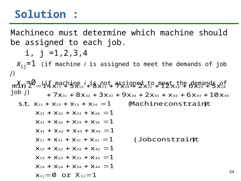
Solution :
Machineco must determine which machine should be assigned to each job. i, j =1,2,3,4 xij=1 (if machine i is assigned to meet the demands of job j)
xij=0 (if machine i is not assigned to meet the demands of job j)
1X or 0x
1xxxx
1xxxx
1xxxx
)constraint (Job1xxxx
1xxxx
1xxxx
1xxxx
)constraintMachine(1xxxx .t.s
x10x6xx2x9x3x8x7
x5x6x12x2x7x8x5x14Zmin
ijij
44342414
43332313
42322212
41312111
44434241
34333231
24232221
14131211
4443424134333231
2423222114131211
65
指派問題之求解方法
Simplex method ( 單體法 ) Transportation Simplex Method ( 運輸單體法 ) Hungarian Method ( 匈牙利法 )

66
Initial Solution — Minimum Coat Method
Table 44 J1 J2 J3 J4 supply
M1
14 5 8 71
M2
2 12 6 51
M3
7 8 3 91
M4
2 4 6 101
demand 1 1 1 1
67
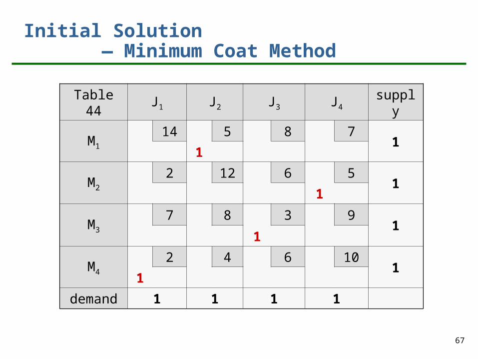
Initial Solution — Minimum Coat Method
Table 44 J1 J2 J3 J4 supply
M1
14 5 8 71
1
M2
2 12 6 51
1
M3
7 8 3 91
1
M4
2 4 6 101
1
demand 1 1 1 1
68
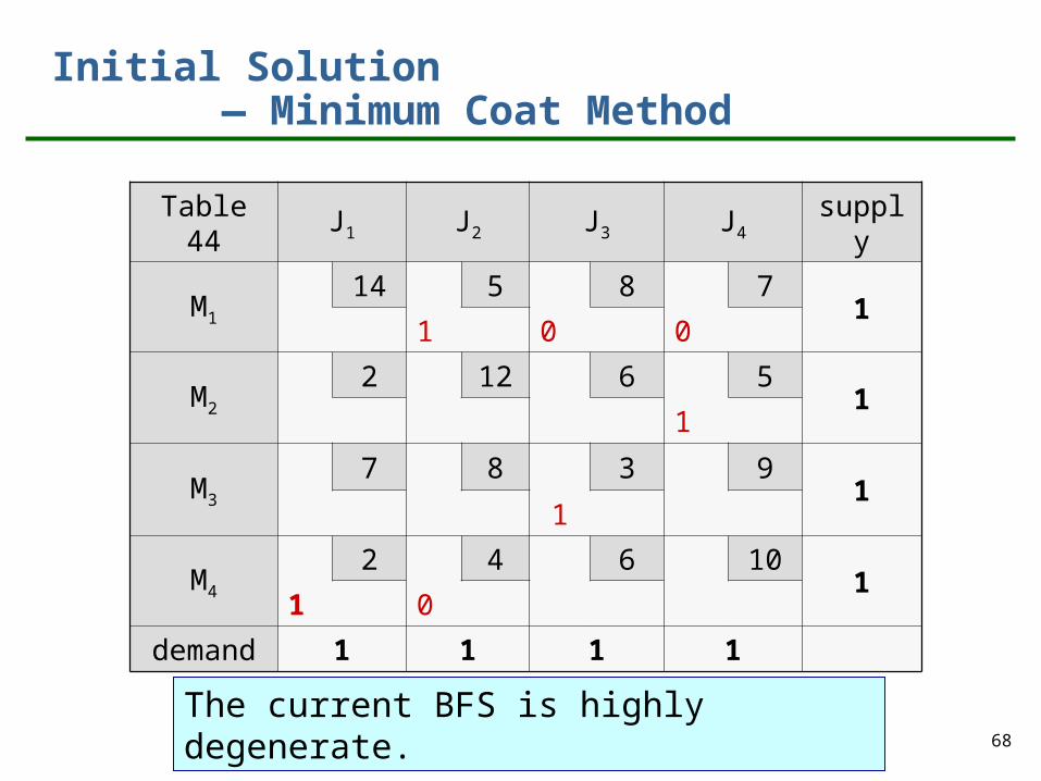
Initial Solution — Minimum Coat Method
Table 44 J1 J2 J3 J4 supply
M1
14 5 8 71
1 0 0
M2
2 12 6 51
1
M3
7 8 3 91
1
M4
2 4 6 101
1 0
demand 1 1 1 1
The current BFS is highly degenerate.
69
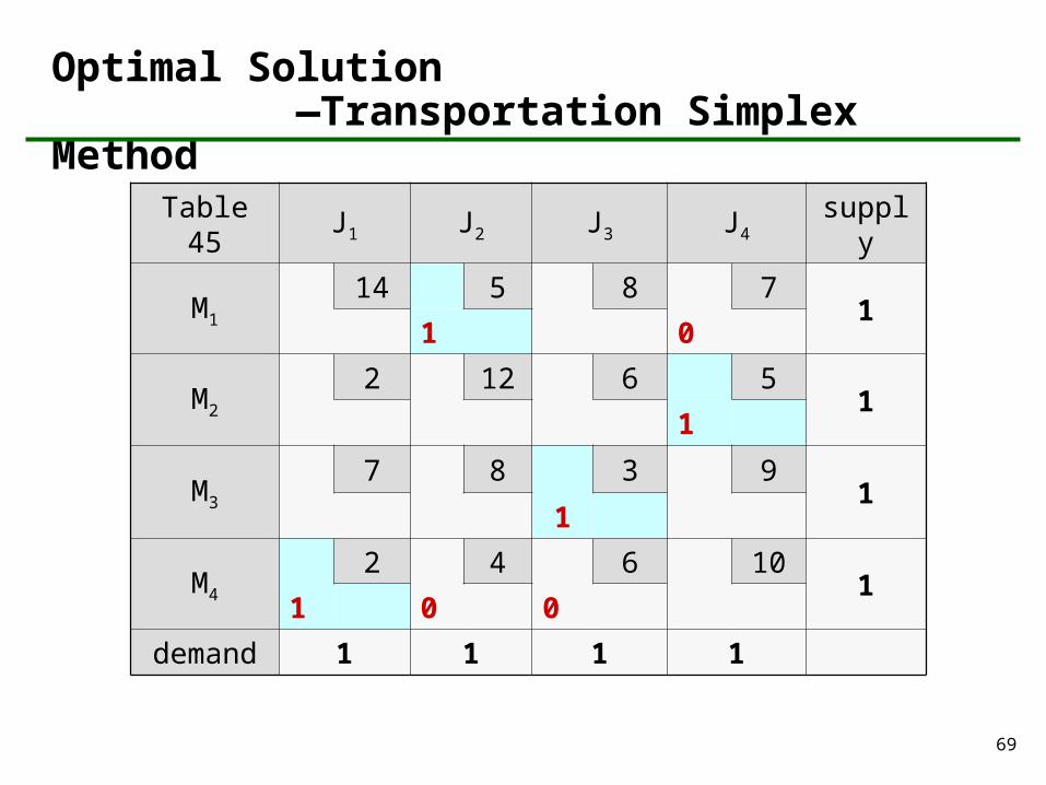
Optimal Solution —Transportation Simplex Method
Table 45 J1 J2 J3 J4 supply
M1
14 5 8 71
1 0
M2
2 12 6 51
1
M3
7 8 3 91
1
M4
2 4 6 101
1 0 0
demand 1 1 1 1
70
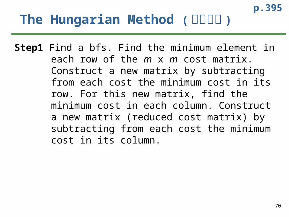
The Hungarian Method ( 匈牙利法 )
Step1 Find a bfs. Find the minimum element in each row of the m x m cost matrix. Construct a new matrix by subtracting from each cost the minimum cost in its row. For this new matrix, find the minimum cost in each column. Construct a new matrix (reduced cost matrix) by subtracting from each cost the minimum cost in its column.
p.395
71
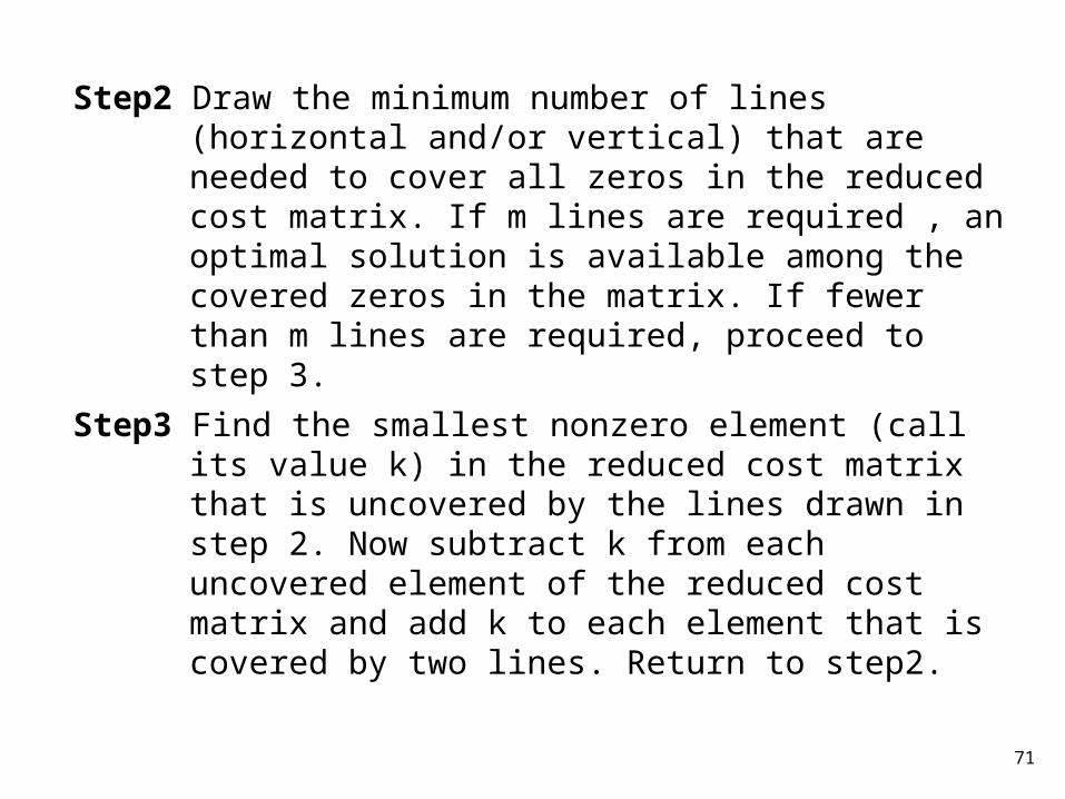
Step2 Draw the minimum number of lines (horizontal and/or vertical) that are needed to cover all zeros in the reduced cost matrix. If m lines are required , an optimal solution is available among the covered zeros in the matrix. If fewer than m lines are required, proceed to step 3.
Step3 Find the smallest nonzero element (call its value k) in the reduced cost matrix that is uncovered by the lines drawn in step 2. Now subtract k from each uncovered element of the reduced cost matrix and add k to each element that is covered by two lines. Return to step2.

72
匈牙利法之步驟
1.建立成本表:方陣2.簡化列:列- row min
3.簡化行:行- col min
4.最佳測試性:最少劃 0 線 , 若線條數 = 列數 , 則進行指派5.進一步簡化成本表
(a) 未劃線元素 - 最小未劃線元素(b) 劃二線元素 + 最小未劃線元素(c) 返回 4.
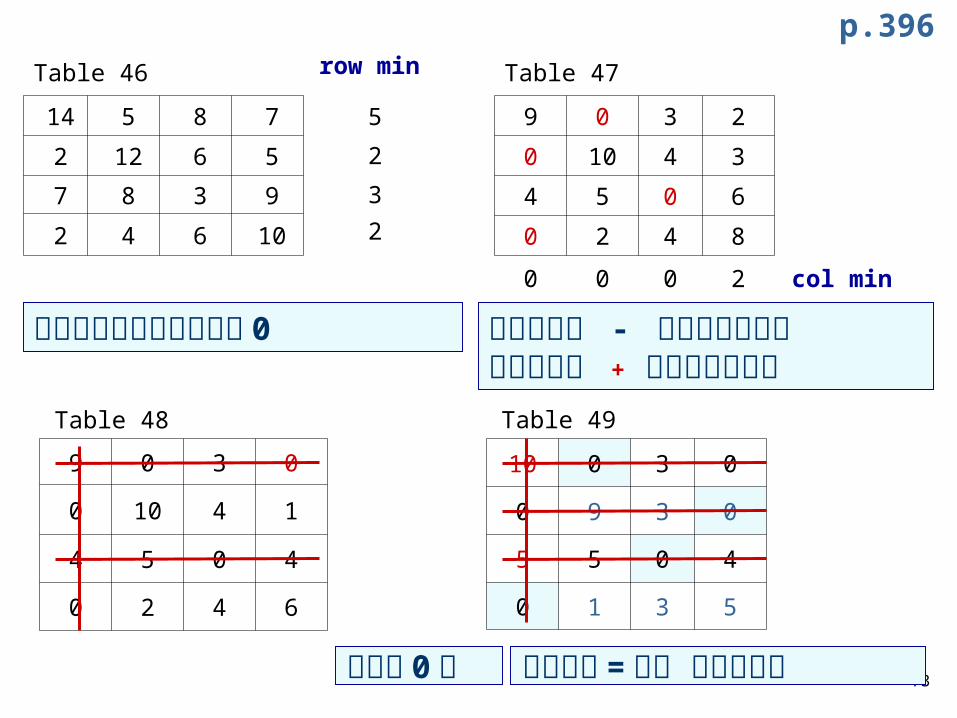
73
row min
5
2
3
2
Table 46
14 5 8 7
2 12 6 5
7 8 3 9
2 4 6 10
Table 47
9 0 3 2
0 10 4 3
4 5 0 6
0 2 4 8
Table 48
9 0 3 0
0 10 4 1
4 5 0 4
0 2 4 6
以最少之線條劃過所有的 0
Table 49
10 0 3 0
0 9 3 0
5 5 0 4
0 1 3 5
未劃線元素 - 最小未劃線元素劃二線元素 + 最小未劃線元素
p.396
最少劃 0線
若線條數 = 列數 則進行指派
0 0 0 2 col min

74
Exercise : p.398 #1 Optimal Solution -The Hungarian Method
Table 50J1 J2 J3 J4 J5 Row Min
P1 22 18 30 18 0 0P2 18 M 27 22 0 0P3 26 20 28 28 0 0P4 16 22 M 14 0 0P5 21 M 25 28 0 0
Col Min 16 18 25 14 0
J1 J2 J3 J4 J5P1 6 0 5 4 0P2 2 M 2 8 0P3 10 2 3 14 0P4 0 4 M 0 0P5 5 M 0 14 0

75
J1 J2 J3 J4 J5P1 6 0 5 4 0P2 2 M 2 8 0P3 10 2 3 14 0P4 0 4 M 0 0P5 5 M 0 14 0
J1 J2 J3 J4 J5P1 6 0 7 4 2P2 0 M 2 6 0P3 8 0 3 12 0P4 0 4 M 0 2P5 3 M 0 12 0
#(col)=5#(line)=4
The smallest uncovered element is 2.
#(col)=5#(line)=5
An optimal solution is available.
Subtract 2 from uncovered costs.Add 2 to all twice covered cost.

76
J1 J2 J3 J4 J5
P1 6 0 7 4 2
P2 0 M 2 2 0
P3 8 0 3 12 0
P4 0 4 M 0 2
P5 3 M 0 12 0
J1 J2 J3 J4 J5
P1 6 0 7 4 2
P2 0 M 2 2 0
P3 8 0 3 12 0
P4 0 4 M 0 2
P5 3 M 0 12 0
J1 J2 J3 J4 J5
P1 6 0 7 4 2
P2 0 M 2 2 0
P3 8 0 3 12 0
P4 0 4 M 0 2
P5 3 M 0 12 0
J1 J2 J3 J4 J5
P1 6 0 7 4 2
P2 0 M 2 2 0
P3 8 0 3 12 0
P4 0 4 M 0 2
P5 3 M 0 12 0
Person 3 is not assigned any job.Total time =18+18+14+25=75
Assignment
77
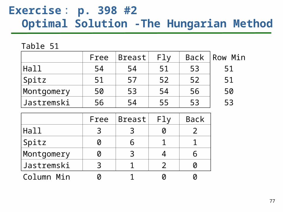
Free Breast Fly Back
Hall 3 3 0 2
Spitz 0 6 1 1
Montgomery 0 3 4 6
Jastremski 3 1 2 0
Column Min 0 1 0 0
Table 51Free Breast Fly Back Row Min
Hall 54 54 51 53 51Spitz 51 57 52 52 51Montgomery 50 53 54 56 50Jastremski 56 54 55 53 53
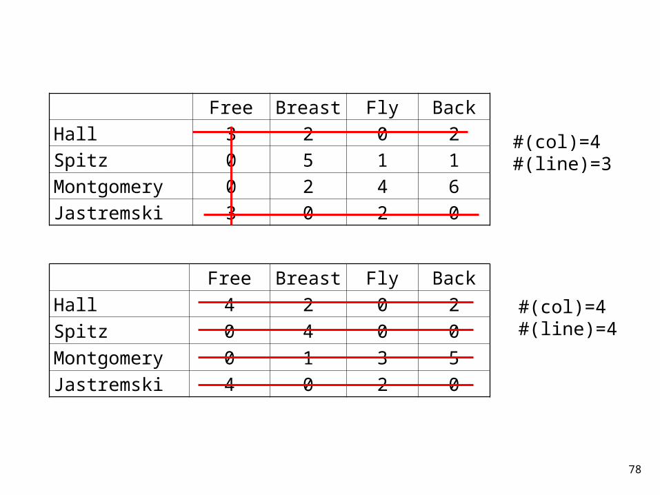
Exercise : p. 398 #2 Optimal Solution -The Hungarian Method
78
Free Breast Fly BackHall 3 2 0 2Spitz 0 5 1 1Montgomery 0 2 4 6Jastremski 3 0 2 0
Free Breast Fly BackHall 4 2 0 2Spitz 0 4 0 0Montgomery 0 1 3 5Jastremski 4 0 2 0
#(col)=4#(line)=3
#(col)=4#(line)=4

79
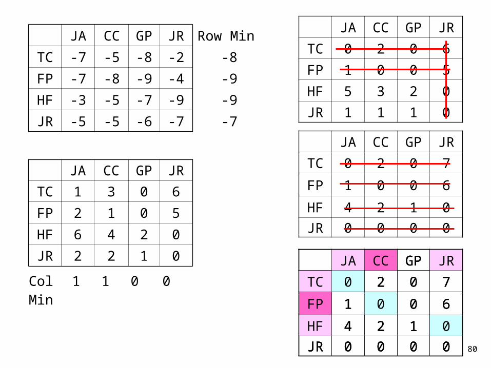
Exercise : p. 399 #3a Optimal Solution -The Hungarian Method
max z=7x11 + 5x12 + 8x13 + 2x14 +... + 5x41 + 5x42 + 6x43 + 7x44
s.t x11 + x12 + x13 + x141 (TC) x21 + x22 + x23 + x241 (FP) x31 + x32 + x33 + x341 (HF) x41 + x42 + x43 + x441 (ML) x11 + x21 + x31 + x411 (JA) x12 + x22 + x32 + x421 (CC) x13 + x23 + x33 + x431 (GP) x14 + x24 + x34 + x441 (JR) xij0
JA CC GP JR
TC -7 -5 -8 -2
FP -7 -8 -9 -4
HF -3 -5 -7 -9
JR -5 -5 -6 -7
Transform Max problem to Min problem, Multiplying benefits by (‑1).
Table 52
JA CC GP JR
TC 7 5 8 2
FP 7 8 9 4
HF 3 5 7 9
JR 5 5 6 7
80
JA CC GP JR
TC 1 3 0 6
FP 2 1 0 5
HF 6 4 2 0
JR 2 2 1 0
JA CC GP JR Row Min
TC -7 -5 -8 -2 -8
FP -7 -8 -9 -4 -9
HF -3 -5 -7 -9 -9
JR -5 -5 -6 -7 -7
JA CC GP JR
TC 0 2 0 6
FP 1 0 0 5
HF 5 3 2 0
JR 1 1 1 0
Col 1 1 0 0Min
JA CC GP JR
TC 0 2 0 7
FP 1 0 0 6
HF 4 2 1 0
JR 0 0 0 0
JA CC GP JR
TC 0 2 0 7
FP 1 0 0 6
HF 4 2 1 0
JR 0 0 0 0
JA CC GP JR
TC 0 2 0 7
FP 1 0 0 6
HF 4 2 1 0
JR 0 0 0 0
JA CC GP JR
TC 0 2 0 7
FP 1 0 0 6
HF 4 2 1 0
JR 0 0 0 0

81
7.6 Transshipment Problems
A transportation problem( 轉運問題 ) allows only shipments that go directly from supply points to demand points.
Shipments are allowed between supply points or between demand points.
Sometimes there may also be points (called transshipment points) through which goods can be transshipped on their journey from a supply point to a demand point.
Fortunately, the optimal solution to a transshipment problem can be found by solving a transportation problem.
p.400

82
Step 1 If necessary, add a dummy demand point
(with a supply of 0 and a demand equal to the problem’s excess supply) to balance the problem. Shipments to the dummy and from a point to itself will be zero. Let s= total available supply.
Step2 Construct a transportation tableau as follows: A row in the tableau will be needed for each supply point and transshipment point, and a column will be needed for each demand point and transshipment point.
83
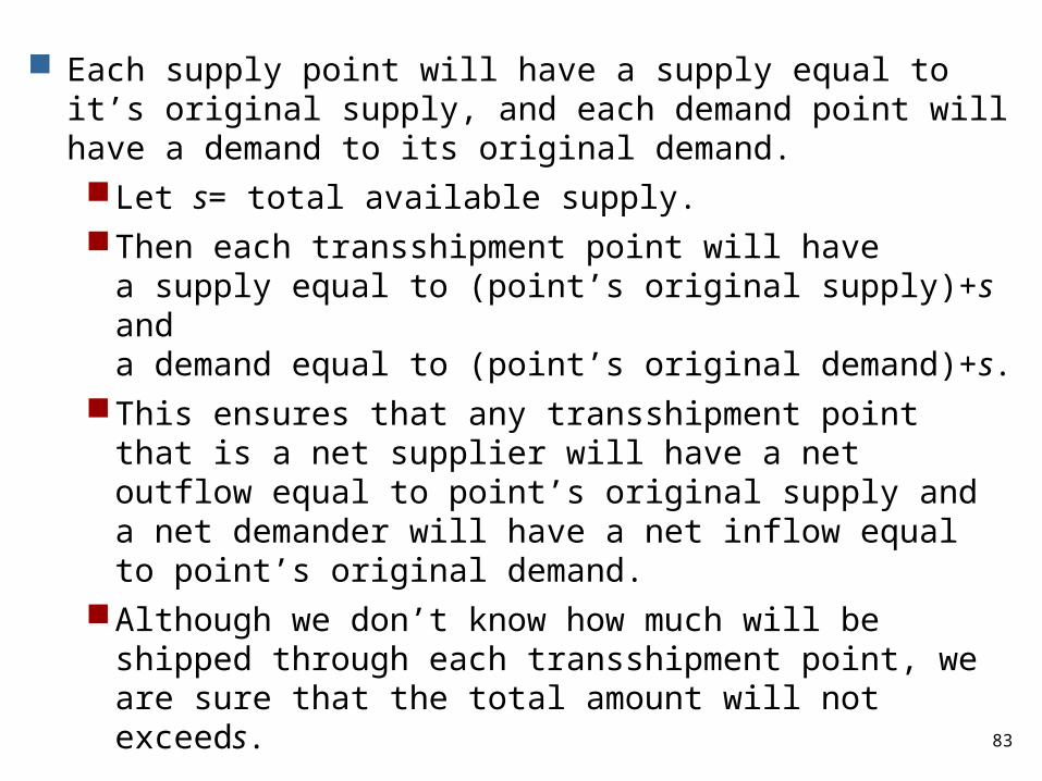
Each supply point will have a supply equal to it’s original supply, and each demand point will have a demand to its original demand. Let s= total available supply. Then each transshipment point will have
a supply equal to (point’s original supply)+s and a demand equal to (point’s original demand)+s.
This ensures that any transshipment point that is a net supplier will have a net outflow equal to point’s original supply and a net demander will have a net inflow equal to point’s original demand.
Although we don’t know how much will be shipped through each transshipment point, we are sure that the total amount will not exceeds.
84
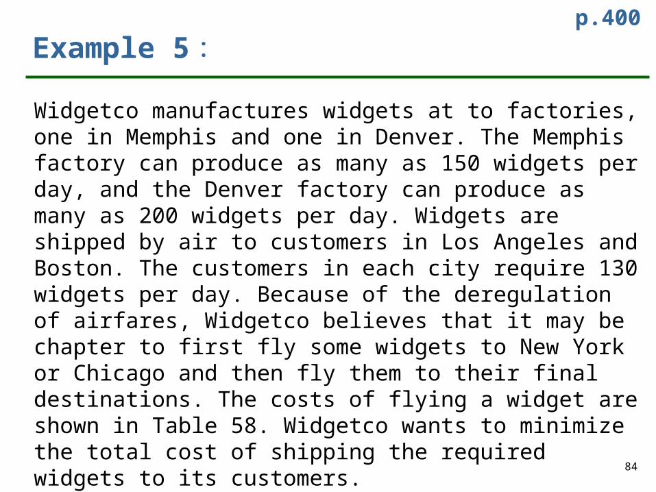
Example 5 :
Widgetco manufactures widgets at to factories, one in Memphis and one in Denver. The Memphis factory can produce as many as 150 widgets per day, and the Denver factory can produce as many as 200 widgets per day. Widgets are shipped by air to customers in Los Angeles and Boston. The customers in each city require 130 widgets per day. Because of the deregulation of airfares, Widgetco believes that it may be chapter to first fly some widgets to New York or Chicago and then fly them to their final destinations. The costs of flying a widget are shown in Table 58. Widgetco wants to minimize the total cost of shipping the required widgets to its customers.
p.400
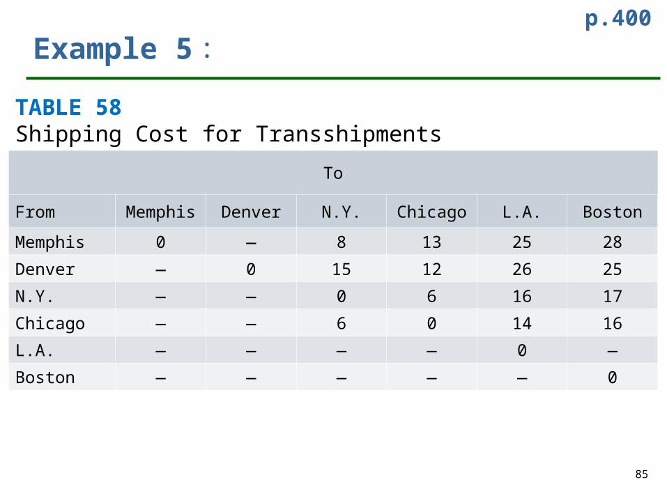
85
Example 5 :p.400
TABLE 58Shipping Cost for Transshipments
To
From Memphis Denver N.Y. Chicago L.A. Boston
Memphis 0 — 8 13 25 28
Denver — 0 15 12 26 25
N.Y. — — 0 6 16 17
Chicago — — 6 0 14 16
L.A. — — — — 0 —
Boston — — — — — 0

86
Figure 9A graphical representation of possible shipments
Memphis N.Y.
Denver Chicago Boston
L.A.
87
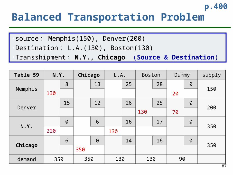
Balanced Transportation Problem
•source : Memphis(150), Denver(200)•Destination : L.A.(130), Boston(130)•Transshipment : N.Y., Chicago (Source & Destination)
Table 59 N.Y. Chicago L.A. Boston Dummy supply
Memphis8 13 25 28 0
150130 20
Denver15 12 26 25 0
200130 70
N.Y.0 6 16 17 0
350220 130
Chicago6 0 14 16 0
350350
demand 350 350 130 130 90
p.400

88
Figure 10Optimal Solution to Widgetco
Memphis N.Y.
Denver Chicago Boston
L.A.130 130
130

89
Exercise : p.403 #1a
Table 60
LA Detroit Atlanta Houston Tampa supplyLA 0 140 100 90 225 1100
Detroit 145 0 111 110 119 2900
Atlanta 105 115 0 113 78Houston 89 109 121 0 -Tampa 210 117 82 - 0demand 2400 1500
LA Detroit Atlanta Houston Tampa Dummy supplyLA 0 140 100 90 225 0 5100Detroit 145 0 111 110 119 0 6900Atlanta 105 115 0 113 78 0 4000Houston 89 109 121 0 M 0 4000Tampa 210 117 82 M 0 0 4000
4000 4000 4000 6400 5500 100
90
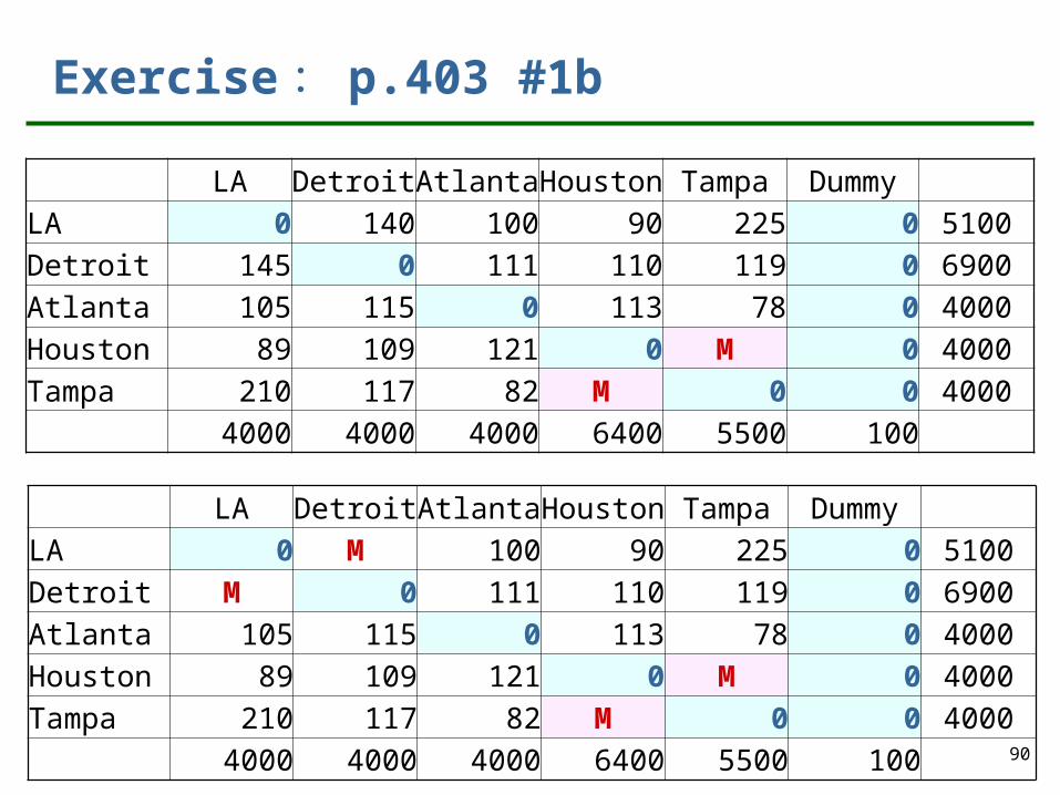
Exercise : p.403 #1b
LA Detroit Atlanta Houston Tampa DummyLA 0 140 100 90 225 0 5100Detroit 145 0 111 110 119 0 6900Atlanta 105 115 0 113 78 0 4000Houston 89 109 121 0 M 0 4000Tampa 210 117 82 M 0 0 4000
4000 4000 4000 6400 5500 100
LA Detroit Atlanta Houston Tampa DummyLA 0 M 100 90 225 0 5100Detroit M 0 111 110 119 0 6900Atlanta 105 115 0 113 78 0 4000Houston 89 109 121 0 M 0 4000Tampa 210 117 82 M 0 0 4000
4000 4000 4000 6400 5500 100

91
Exercise : p.403 #2Table 61
Well1 Well2 Mobile Galv. N.Y. L.A.Well 1 0 - 10 13 25 28 150Well 2 - 0 15 12 26 25 200Mobile - - 0 6 16 17Galv. - - 6 0 14 16N.Y. - - - - 0 15L.A. - - - - 15 0
140 160
Mobile Galv. N.Y. L.A. Dummy supplyWell 1 10 13 25 28 0 150Well 2 15 12 26 25 0 200Mobile 0 6 16 17 0 350Galv. 6 0 14 16 0 350N.Y. M M 0 15 0 350L.A. M M 15 0 0 350demand 350 350 490 510 50 1050
92
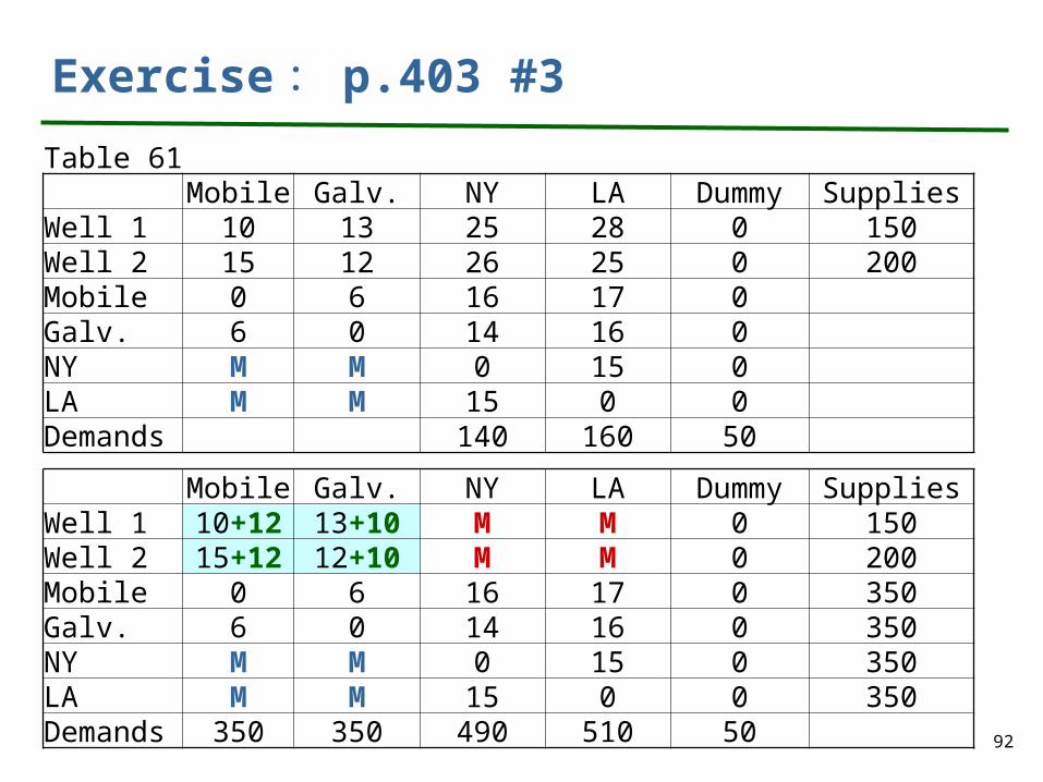
Exercise : p.403 #3
Table 61Mobile Galv. NY LA Dummy Supplies
Well 1 10 13 25 28 0 150Well 2 15 12 26 25 0 200Mobile 0 6 16 17 0Galv. 6 0 14 16 0NY M M 0 15 0LA M M 15 0 0Demands 140 160 50
Mobile Galv. NY LA Dummy SuppliesWell 1 10+12 13+10 M M 0 150Well 2 15+12 12+10 M M 0 200Mobile 0 6 16 17 0 350Galv. 6 0 14 16 0 350NY M M 0 15 0 350LA M M 15 0 0 350Demands 350 350 490 510 50

93
Exercise : p.403 #4
Mobile Galv. NY LA Dummy SuppliesWell 1 10+12 13+10 M M 0 150Well 2 15+12 12+10 M M 0 200Mobile 0 6 16 17 0Galv. 6 0 14 16 0NY M M 0 15 0LA M M 15 0 0Demands 140 160 50
Mobile Galv. NY LA Dummy SuppliesWell 1 10+12 13+10 M M 0 150Well 2 15+12 12+10 M M 0 200Mobile 0 6 16 17 0 180Galv. 6 0 14 16 0 150NY M M 0 15 0 350LA M M 15 0 0 350Demands 180 150 140 160 50
94
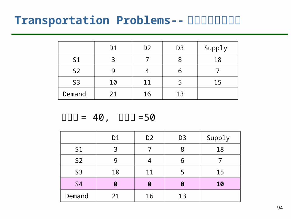
Transportation Problems-- 總供給小於總需求
D1 D2 D3 Supply
S1 3 7 8 18
S2 9 4 6 7
S3 10 11 5 15
Demand 21 16 13
D1 D2 D3 Supply
S1 3 7 8 18
S2 9 4 6 7
S3 10 11 5 15
S4 0 0 0 10
Demand 21 16 13
總供給 = 40, 總需求 =50

95
Transportation Problems-- 總供給大於總需求
D1 D2 D3 Supply
S1 3 7 8 21
S2 9 4 6 16
S3 10 11 5 13
Demand 18 7 15
D1 D2 D3 D4 Supply
S1 3 7 8 0 18
S2 9 4 6 0 7
S3 10 11 5 0 15
Demand 21 16 13 10
總供給 = 50, 總需求 =40

96
Example: 總供給大於總需求
若來源貨物無法送出時,分別導致每單位 3 、 1 、 2 的存貨成本
D1 D2 D3 D4 Supply
S1 3 7 8 0 18
S2 9 4 6 0 7
S3 10 11 5 0 15
Demand 21 16 13 10 50
D1 D2 D3 D4 Supply
S1 3 7 8 3 18
S2 9 4 6 1 7
S3 10 11 5 2 15
Demand 21 16 13 10 50

97
Example: 總供給大於總需求
若 S1 之貨物必須全部送出,以便挪出空間作為他用
D1 D2 D3 D4 Supply
S1 3 7 8 0 18
S2 9 4 6 0 7
S3 10 11 5 0 15
Demand 21 16 13 10 50
D1 D2 D3 D4 Supply
S1 3 7 8 M 18
S2 9 4 6 0 7
S3 10 11 5 0 15
Demand 21 16 13 10 50
98
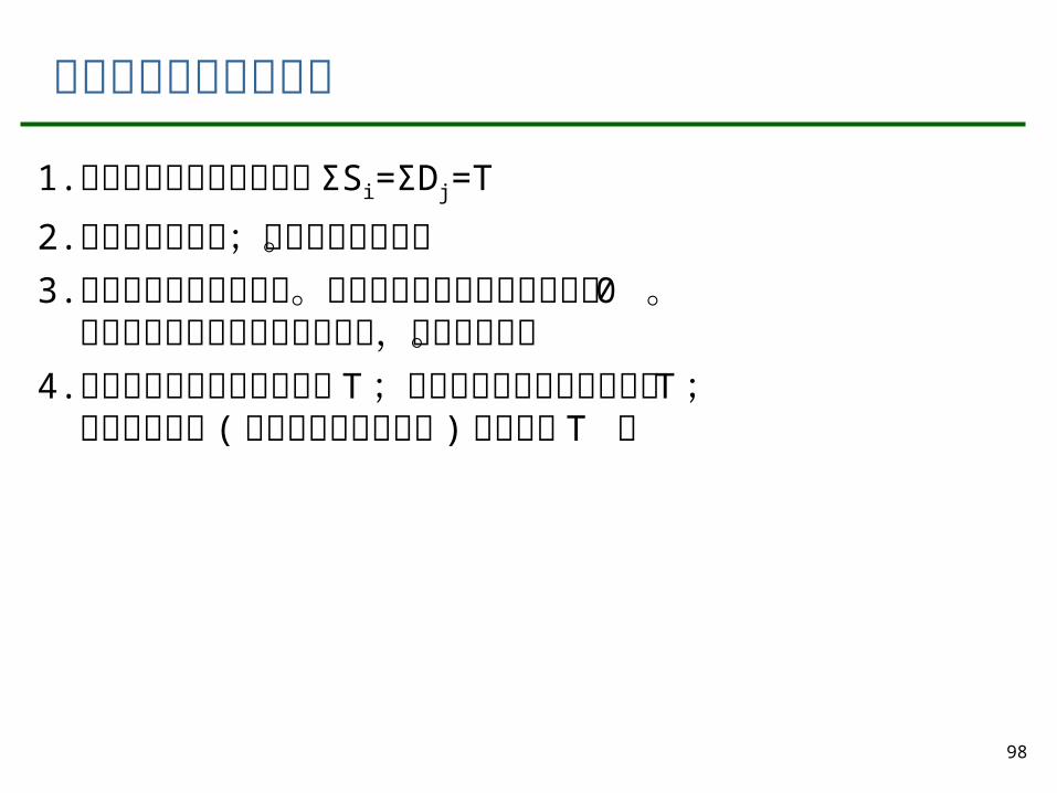
建立轉運供需表之步驟
1.建立平衡之轉運供需表, ΣSi=ΣDj=T
2.增設來源地於列;增設目的地於行。3.填入各路徑之單位成本。通常本站到本站之單位成本為 0 。
任兩點來回之單位成本可能相同,也可能不相。4.可供轉運之起點供給量增加 T ;可供轉運之終點供給量增加 T ;
所有新增之點 ( 無論供給量或需求量 ) 其量均為 T 。

99
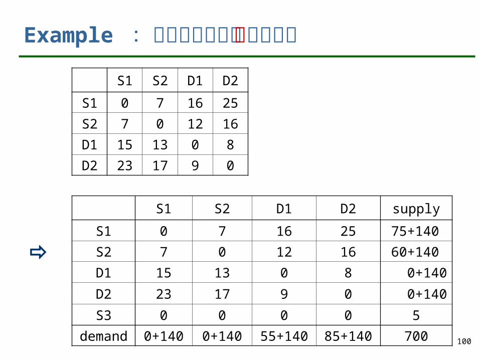
來源地 (S1,S2) 與目的地 (D1,D2) 之供給與需求為: s1=75, s2=60, d1=55, d2=85 。其運輸成本表為如下,則轉運供需表為何?
Example :來源地與目的地不為轉運點
S1 S2 D1 D2
S1 0 7 16 25
S2 7 0 12 16
D1 15 13 0 8
D2 23 17 9 0
D1 D2 supply
S1 16 25 75
S2 12 16 60
S3 0 0 5
demand 55 85 140
100
Example :來源地與目的地均為轉運點
S1 S2 D1 D2
S1 0 7 16 25
S2 7 0 12 16
D1 15 13 0 8
D2 23 17 9 0
S1 S2 D1 D2 supply
S1 0 7 16 25 75+140
S2 7 0 12 16 60+140
D1 15 13 0 8 0+140
D2 23 17 9 0 0+140
S3 0 0 0 0 5
demand 0+140 0+140 55+140 85+140 700