Chapter 7. What Can Neuroeconomics Tell Us About Economics

(and Vice Versa)?

Mark Dean

May 11, 2012

Neuroeconomics is now a relatively well established discipline at the intersection of neuroscience,

psychology and economics. It has its own societies, conferences, textbooks1 and graduate courses.

The number of articles2 that contain the word �neuroeconomics�has grown from essentially zero

in 2000 to around 900 a year in 2009 and 2010. The mainstream media has found the concept

of neuroeconomics fascinating, with articles regularly appearing in many major newspapers and

magazines. The idea that we may be able to say something about the biological basis of economic

decision making seems to be both compelling and important.

Yet within economic departments, the potential bene�ts of neuroeconomics are hotly debated.

An amazing amount of light and heat has been generated in arguments about how useful it is for

economists to make use of neuroscience in their everyday business. For a discipline that generally

claims to dislike methodological discussion, we have created a staggering amount of verbiage on

this particular issue. Indeed, the question of whether neuroeconomics is useful has its own textbook

and conferences (though we have stopped short of giving it its own society).

1"Neuroeconomics: Decision Making and the Brain", Glimcher et al. [2008].2According to Google Scholar

1

This chapter represents an addition to the already crowded �eld of discussions on the value of

neuroeconomics.3 In it, I am going to try to make two distinct, but related points. In the �rst

section, I discuss the ways that neuroeconomics (broadly de�ned) has been used to improve our

models of economic choice, and the criticisms of these approaches that have come from economists.

I will claim that there is no reason in principle why an understanding of the neuroscience of decision

making cannot help us make better models of economic choice, and there are good reasons to think

that it can. An understanding of how the brain works can, in principle, �inspire�us to build better

models of economic choice. Moreover, the type of rich data that neuroscientists have at their

disposal o¤er us the possibility of building these models �piece by piece�, rather than all at once.

However, the fact that 10 years of research has generated relatively few ideas that have percolated

up from neuroeconomics to the wider economic community suggests that the task is not an easy

one. Furthermore, the criticisms of the neuroeconomic agenda that have been levelled by the wider

economic community are valuable in pointing out why some of the work carried out in the name

of neuroeconomics is unlikely to move forward our understanding of economics. These criticisms

apply particularly to papers that claim to use neuroeconomic data to test existing economic models

of decision making.

My second point is about how neuroeconomics research is conducted, and particular how to

manage the relationship between theory and data. The question of whether or not neuroeconomics

can help economists with their models is, of course, distinct to the question of whether it is good

science, and there is little doubt that (self identi�ed) neuroeconomists have done great work in

3There are already a large number of fantastic articles on this subject, starting with Camerer, Loewenstein and

Prelec [2004; 2005], then Gul and Pesendorfer [2008], Caplin [2008] (both of which appear in Caplin and Schotter

[2008], which is essentially devoted to the topic), Harrison [2008], Rustichini [2009], Glimcher [2010], Bernheim [2010],

and Ross [2010]

2

advancing our understanding of the processes that underlie simple decision making.4 Yet many

neuroeconomic projects are coming up against a set of data theoretic problems that are familiar

to economists. While neuroeconomic models aim to describe the process by which choices are

made, in practice most retain the �as if��avor familiar that characterize many economic models:

just as economists ask whether choices behave as if they result from the maximization of some

utility function, so neuroeconomists ask whether the lateral intraparietal area (LIP) acts as if

it encodes normalized expected utility, or whether the nucleus accumbens acts as if it encodes

reward prediction error. This is because most neuroeconomic models are couched in terms of

variables that are latent, or unobservable - such as rewards, beliefs, utilities and so on. Such

latent variables are often useful for capturing the intuition behind a model, yet understanding the

observable implications of such models is not always an easy task. This problem is compounded by

the fact that neuroeconomics is speci�cally interdisciplinary, covering di¤erent �levels�of modeling.

The concepts and abstractions that are familiar at one level of analysis may be completely alien at

another. As pointed out by Glimcher [2010] and Caplin [2008], the real bene�ts of interdisciplinary

research will only come when everyone is working with the same objects.

The second section of this chapter will make the case that, in order to understand the testable

implications of their models, neuroeconomics can bene�t from a common modelling technique

in economics - the use of �axioms�, or simple rules to capture non-parametrically the testable

implications of models that contain latent variables. These techniques (used in economics since

the seminal work of Samuelson [1938]) require one to de�ne precisely the role of one�s abstractions

within a model. This forces researchers from di¤erent disciplines to agree on the properties of

these abstractions, or at least recognize that they are dealing with di¤erent objects. Moreover,

once a model has been agreed upon, the axiomatic technique provides a way of understanding the

4For recent overviews, see Glimcher [2010] and Fehr and Rangel [2011].

3

testable implications of the model for di¤erent data sets, without the need for additional auxiliary

assumptions. Put another way, they identify the testable implications of an entire class of models

(such as utility maximization) without needing to specify the precise form of the latent variables

(such as utility). I illustrate this approach using the work of Caplin, Dean, Glimcher and Rutledge

[2010], who use it to test whether the nucleus accumbens encodes a reward prediction error - a key

algorithmic component in models of learning and decision making.

This chapter is not intended to be a comprehensive survey of the neuroeconomic literature, and

as such does a disservice to many valuable contributions to the neuroeconomic canon. This includes

foundational work on how simple choices are instantiated in the brain [for example Sugrue et al.

2005; Padoa-Schioppa and Assad 2006; Rangel et al. 2008; Wunderlich et al. 2009], the neuroscience

of decision making in risky situations [Hsu et al. 2005; Preuscho¤ et al. 2006; Bossaerts et al.

2008; Levy et al 2010], intertemporal choice [Kable and Glimcher; 2007], choice in social settings

[DeQuervain et al. 2004; Fehr et al. 2005; Knoch et al. 2006; Hare et al. 2010; Tricomi et al.

2010] and choices involving temptation and self control [Hare et al. 2009]. There is also a truly

enormous literature on the neuroscience of learning which has interesting links to economic issues

(see Glimcher [2011] for a recent review). For a more comprehensive review of the state of the

art in neuroeconomics, see the recent review article of Fehr and Rangel [2011] or the textbook

�Neuroeconomics: Decision Making and the Brain�edited by Glimcher et al. [2008].

1 What is Neuroeconomics?

Part of the debate about the usefulness or otherwise of neuroeconomics stems from the fact that

there are (at least) three distinct intellectual projects that fall under the heading. One way to

group these projects is as follows

4

1. To improve model of economic choice by explicitly modelling the process by which these

choice are made, and using non-standard data in order to test these process models. This

non-standard data might be in the form of measurement of brain activity using functional

magnetic resonance imaging (fMRI), but might also include less dramatic examples such as

reaction times, eye tracking, etc.5

2. To model the neurobiological mechanisms that are responsible for making (economic) choices.

These models may be based on existing modeling frameworks within economics. In contrast

to (1) above, here, the understanding of the process by which choices are made is the aim in

and of itself, rather than an input into the project of understanding economic choice.

3. To use non-standard data (again, including, but not restricted to brain activation) to make

normative statements about the desirability of di¤erent outcomes. In other words, to move

beyond the �revealed preference�paradigm that is prevalent in economics, and use data other

than choices alone to make welfare comparisons.

This chapter is largely concerned with the �rst two of these projects. In the �rst section I will

explicitly discuss the feasibility of the �rst aim. In the second, I discuss how the axiomatic approach

can be applied to testing neuroeconomic models of process, whether the process model is the end

5Often, �neuroeconomics� is more narrowly de�ned as studies that use measurements or manipulations of the

brain during economic tasks. Measurement of brain activity (the most common approach) is usually done using

functional Magnetic Resonance Imaging (fMRI) or Electroencephalography (EEG) in humans, or recording from a

single neuron in animals. However, other techniques are also used in order to establish causal links, including the

use of lesion patients (who have damage to a particular brain area), Transcranial Magnetic Stimulation (TMS) which

temporarily disrupts activity in a brain area, and pharmacalogical interventions that raise or lower the activity of

a neurotransmitter. For a more thorough review of the various techniques on o¤er, see Colin Camerer�s chapter in

Caplin and Schotter [2010].

5

in itself, or an input into understanding economic choice.

2 HowCan Neuroeconomics ImproveModels of Economic Choice?

In order to address the question of how neuroscience can help us build better models of economic

decision making, it is necessary to understand what we mean by �economic decision making�. Clearly

this concept (or even the concept of a �choice�, as opposed to, say, an unconscious reaction to a

given environment) is a bit fuzzy (see Caplin [2008]), but it is also clear that some behavioral

relationships will interest more economists than others. If we think of a model as a function f that

maps a set of environmental conditions X to a set of behaviors Y ,6 then most economists deal with

X�s that are de�ned by variables such as prices, incomes, information states, etc., and Y �s that are

de�ned as demands for di¤erent types of good and service. So, for example, an economist might be

interested in the relationship between the wages prevalent in the market (environmental conditions

X) and the labour that a worker wants to supply (outcome Y ). The key point is that, for most

economists, X nor Y will contain information of brain activity, eye movements, oxytocin levels and

so forth - the type of data that neuroeconomics typically work with.7

It is important to note that this restriction does not represent narrow mindedness on the part

of economists - it simply re�ects the projects that they are involved in. For example, consider an

economist who wants to understand how a �rm can set its prices to maximize pro�t. In order to

determine this, they will need to know the e¤ect of increasing the price of a good on demand for

that good. This economist may well recognize that there are many intermediate steps between the

policy variable they are interested in (price) and the outcome they are interested in (whether or not

6 for example something that tells us what people choose (outcomes in Y ) when faced with di¤erent prices (envi-

ronmental conditions X)7The formalization, and much of the argument in this section relies heavily on Bernheim [2010]

6

a person buys they good), and these intermediate steps will involve changes in the brain states of

the person in question. However, these brain states represent neither the environmental conditions

nor the behavioral outcomes they are interested in, and with good reason. Firms cannot directly

manipulate the brain states of their customers, nor can they decide what price to charge on the

basis of these brain states.8 Moreover, their pro�ts will depend on whether or not a good is bought,

not brain activity of the customer at the time of purchase. Thus, while measuring brain states may

help this economist in achieving their �nal goal, they are not objects of interest per se.

Arguably the de�ning feature of the neuroeconomic approach is that it takes seriously the fact

that the types of f that economists generally consider are really reduced-form short cuts of the true

underlying process. While the economist may �nd it convenient to imagine a decision maker (DM)

as simply a function that maps market prices to demands, there are clearly a myriad of intermediate

steps underlying this relationship. For example, the DM must collect information on what goods

are available, and the prices of these goods, which must then be combined with information already

stored in the brain to generate some form of rating for each of the a¤ordable bundles of goods. The

resulting data must then be processed in some way to select a course of action.(i.e. what to buy).

In other words, the relationship f is really the reduced form of a chain of mappings

h1 : X ! Z1

h2 : Z1 ! Z2

...

hn : Zn ! Y

8Of course, they may be able to indirectly manipulate the brain states of the customer through, for example,

advertising. In such cases economists and marketing scientists may include types of advertising stimuli in their set

of interesting environmental parameters X.

7

so that f = hn:hn�1:::h1. These hi�s form the intermediate steps in the decision making process,

and the Zi�s form the intermediate variables that get handed from one stage of the process to the

next. So, for example, h1 could be the mapping from a display of prices (X) to retinal activation

(Z1) which in turn maps to activation in the visual cortex (h2 : Z1 ! Z2), which leads to activity

in the ventral striatum (h3 : Z2 ! Z3), which activates brain area M1 (h4 : Z3 ! Z4), which leads

to an arm movement (h4 : Z3 ! Z4) and the purchase of a good (h5 : Z4 ! Y ).

Crucially, these intermediate stages can contain variables which are not of immediate interest

to traditional economists - (brain activity, eye movements, oxytocin levels and so forth). But (for

the purposes of this chapter), it is still the function f that is the object of interest. Of course, the

exact number of steps n is ill de�ned: any given h could be further broken down into subprocesses

- for example to the level of di¤erent neurons talking to each other. For simplicity, we will consider

a two stage model

h : X ! Z

g : Z ! Y

such that f = h:g:9 The key question of this section is therefore whether explicitly modelling

the relationships h and g, and measuring Z is a useful thing to do if what you are really interested

in is the relationship f:

9Of course, the question of how and when to aggregate intermediate steps in a model - i.e. when to treat an h and

a g as a single f - is not unique to neuroeconomics. For example, in international politics, one often studies decisions

by governments as if they were unitary actors, and so can have their preferences represented by a utility function. As

useful as that approach can be, most people would accept that we can learn by examining how those decisions are

reached through the political process within a government (though people may disagree how much detailed content

of that political process should be included in that disaggregation). Because many decisions we wish to examine are

collective decisions, the choice of whether or not to dissagregate applies to them as well.

8

To some, particularly those based in the biological sciences, the answer to this question is self

evidently �yes�. The analogy is often made between predicting economic choices and predicting what

a computer program will do. One way to learn about a computer program would be to look at the

mapping between inputs to and the outputs from the program - i.e. to type things in and see what

comes out. One could propose models of the relationship between inputs to and outputs from the

program, and test these models on this data. However, it seems that it would be signi�cantly more

e¢ cient to look at the underlying code of the program to understand what is going on. Moreover,

we might feel more con�dent in making out-of-sample predictions10 of what the computer program

will do if we understand the underlying coding. By analogy, it is surely sensible to understand the

processes underlying choice, rather than simply look at the choices that people make from di¤erent

choice sets. However, as we will see below, not all economists buy this analogy - and their criticisms

are pertinent to those that want to use neuroeconomics to improve our understanding of economic

decision making.

2.1 When Theorists Attack: The Backlash Against Neuroeconomics

The early days of neuroeconomics generated an immense amount of interest within the economics

community.11 Since then, there has been something of a cooling of attitudes amongst many econo-

mists. Part of this may be perceived as a reaction to overblown initial claims of what neuroeconomics

can do [see Harrison 2008]. However, there have also been articles that have attacked the neuroeco-

nomic project as fundamentally �awed, the most famous being �The Case for Mindless Economics�

by Faruk Gul and Wolfgang Pesendorfer [2008].

10 i.e. using our models to make predictions in novel situations11 In 2004, when I �rst began attending the Neuroeconomics Seminar at New York University, economists were

literally standing outside in the corridor half an hour before the seminar because the room was so full.

9

On the face of it, the idea that an understanding of the neural architecture involved in decision

making might help us to model economic choice seems an eminently sensible one. Moreover, the

�reduction�of one level of analysis to another has bourne fruit in many other disciplines - for example

the relationship between neuroscience and chemistry, or the relationship between chemistry and

physics. (Glimcher [2010] elegantly traces the philosophical arguments surrounding reductionism).

So what were the criticisms that economic theorists found so compelling? Essentially, they came

in two related �avors

1. Economists are only interested in the behavioral implications of a model (in our language the

are only interested in the mapping f from X to Y ). Two process models fh; gg and fh0; g0g

either imply di¤erent mappings f and f 0, or they don�t, (so g:h = g0:h0). In the former case,

�standard�economic evidence can be used to di¤erentiate between the two models (i.e. there

is some x in X such that f(x) 6= f 0(x), so we can use such an x to di¤erentiate between

the two models). In the later, as economists, we are not interested in the di¤erence between

fh; gg and fh0; g0g:

2. Economic models make no predictions about process, so observations of process cannot be

used to test economic models. In other words, when economists say that (for example) people

maximize utility, all we mean is that they act as if they make choices in order to maximize

some stable utility function. We are agnostic about whether people are actually calculating

utilities in their heads. So evidence on the existence or otherwise of a utility function in the

brain is neither here nor there.

The �rst thing to note is that both of these criticisms are serious, and should be treated as

such by neuroeconomists who want their work to in�uence the wider economics community. Any

neuroeconomics project designed to improve understanding of economic decision making should be

10

able to address both of them.

The easiest way to illustrate the power of these criticisms is with an example. For this purpouse,

I use the simplest and most pervasive model in economics - that of utility maximization. This

example will also serve to illustrate how economists think about models that have latent variables,

and what we mean by saying that our models are �as if�in �avour.12 As this is the approach that,

in section 2, I claim can be usefully applied to neuroeconomics, I go through the example in some

detail.

2.2 An Example: Utility Maximization and Choice

Arguably the most widely used behavioral model in economics is that of �utility maximization�

- according to which people make choices in order to maximize some stable utility function that

describes how �good� each alternative is. A natural question is: how can we test this model of

choice? The answer to this question (or indeed any question of this type) depends on two elements:

1. The data we wish to explain: In this case, the data will consist of the choices that people

make, and the set of available alternatives that they are choosing from. So, for example, if

we want to model a decision maker�s choices over snack foods, then the data might come in

12Economists are not, of course, a homogeneous mass, and there are a wide variety of di¤erent modelling approaches

used within the discipline. The approach that I describe here is most closely related to a branch of economics known

as �decision theory�.

11

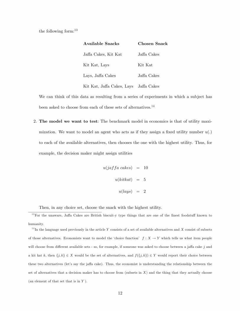
the following form:13

Available Snacks Chosen Snack

Ja¤a Cakes, Kit Kat Ja¤a Cakes

Kit Kat, Lays Kit Kat

Lays, Ja¤a Cakes Ja¤a Cakes

Kit Kat, Ja¤a Cakes, Lays Ja¤a Cakes

We can think of this data as resulting from a series of experiments in which a subject has

been asked to choose from each of these sets of alternatives.14

2. The model we want to test: The benchmark model in economics is that of utility maxi-

mization. We want to model an agent who acts as if they assign a �xed utility number u(:)

to each of the available alternatives, then chooses the one with the highest utility. Thus, for

example, the decision maker might assign utilities

u(jaffa cakes) = 10

u(kitkat) = 5

u(lays) = 2

Then, in any choice set, choose the snack with the highest utility.13For the unaware, Ja¤a Cakes are British biscuit-y type things that are one of the �nest foodstu¤ known to

humanity.14 In the language used previously in the article Y consists of a set of available alternatives and X consist of subsets

of those alternatives. Economists want to model the �choice function� f : X ! Y which tells us what item people

will choose from di¤erent available sets - so, for example, if someone was asked to choose between a ja¤a cake j and

a kit kat k, then fj; kg 2 X would be the set of alternatives, and f(fj; kg) 2 Y would report their choice between

these two alternatives (let�s say the ja¤a cake). Thus, the economist is understanding the relationship between the

set of alternatives that a decision maker has to choose from (subsets in X) and the thing that they actually choose

(an element of that set that is in Y ).

12

Notice that there is a feature of this model that makes it di¢ cult to test: we do not directly

observe utilities! If objects had utilities stamped on them, then testing the model would be easy:

we could just look at the choices that a DM makes from di¤erent choice sets, and see if they always

choose the object with highest utility. But in general objects do not have utilities stamped on

them: if I look at a kit kat, I cannot directly observe what its utility is. How can we proceed?

One way to go would be to assume a particular utility function, and test that. For example, we

could assume that people prefer more calories to less, and so utility should be equivalent to calories.

However, there is a problem with this approach: We might pick the wrong utility function. Maybe

the person we are observing is a dieter, and actually prefers less calories to more. Such a person

would be maximizing a utility function, just not the one we assumed. Thus we could wrongly reject

the model of utility maximization.

It would be better if we could ask the question whether there exists any utility function that

explains peoples� choices. Put another way, can we identify patterns of choices that cannot be

explained by the maximization of any utility function? Consider the following choices made by an

experimental subject Ambrose

Ambrose�s Choices

Available Snacks Chosen Snack

Ja¤a Cakes, Kit Kat Ja¤a Cakes

Kit Kat, Lays Kit Kat

Lays, Ja¤a Cakes Lays

Kit Kat, Ja¤a Cakes, Lays Ja¤a Cakes

Is it possible that Ambrose�s choices can be explained by the maximization of some utility

function? The answer is no. If Ambrose is making choices in order to maximize a utility function,

13

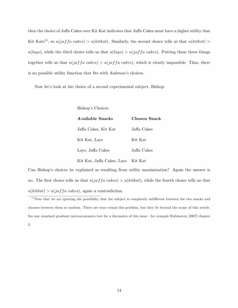
then the choice of Ja¤a Cakes over Kit Kat indicates that Ja¤a Cakes must have a higher utility that

Kit Kats15, so u(jaffa cakes) > u(kitkat). Similarly, the second choice tells us that u(kitkat) >

u(lays), while the third choice tells us that u(lays) > u(jaffa cakes). Putting these three things

together tells us that u(jaffa cakes) > u(jaffa cakes), which is clearly impossible Thus, there

is no possible utility function that �ts with Ambrose�s choices.

Now let�s look at the choice of a second experimental subject, Bishop:

Bishop�s Choices

Available Snacks Chosen Snack

Ja¤a Cakes, Kit Kat Ja¤a Cakes

Kit Kat, Lays Kit Kat

Lays, Ja¤a Cakes Ja¤a Cakes

Kit Kat, Ja¤a Cakes, Lays Kit Kat

Can Bishop�s choices be explained as resulting from utility maximization? Again the answer is

no. The �rst choice tells us that u(jaffa cakes) > u(kitkat), while the fourth choice tells us that

u(kitkat) > u(jaffa cakes), again a contradiction.

15Note that we are ignoring the possibility that the subject is completely indi¤erent between the two snacks and

chooses between them at random. There are ways round this problem, but they lie beyond the scope of this article.

See any standard graduate microeconomics test for a discussion of this issue - for example Rubinstein [2007] chapter

3.

14

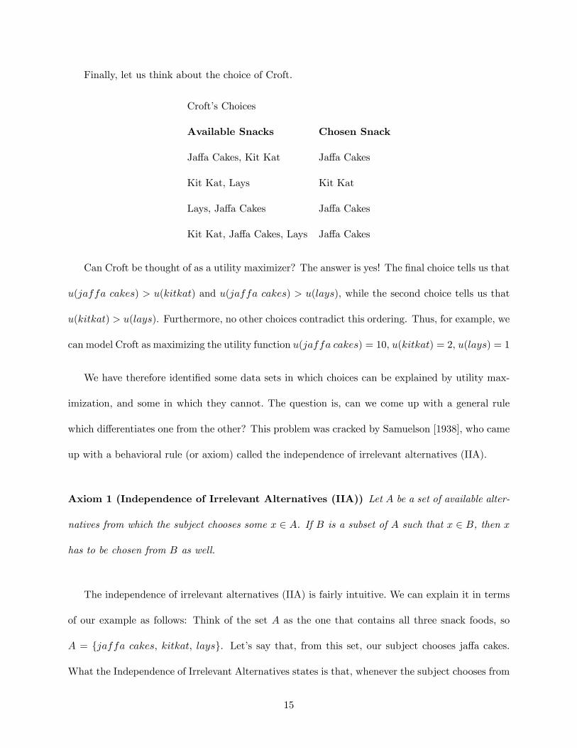
Finally, let us think about the choice of Croft.

Croft�s Choices

Available Snacks Chosen Snack

Ja¤a Cakes, Kit Kat Ja¤a Cakes

Kit Kat, Lays Kit Kat

Lays, Ja¤a Cakes Ja¤a Cakes

Kit Kat, Ja¤a Cakes, Lays Ja¤a Cakes

Can Croft be thought of as a utility maximizer? The answer is yes! The �nal choice tells us that

u(jaffa cakes) > u(kitkat) and u(jaffa cakes) > u(lays), while the second choice tells us that

u(kitkat) > u(lays). Furthermore, no other choices contradict this ordering. Thus, for example, we

can model Croft as maximizing the utility function u(jaffa cakes) = 10, u(kitkat) = 2, u(lays) = 1

We have therefore identi�ed some data sets in which choices can be explained by utility max-

imization, and some in which they cannot. The question is, can we come up with a general rule

which di¤erentiates one from the other? This problem was cracked by Samuelson [1938], who came

up with a behavioral rule (or axiom) called the independence of irrelevant alternatives (IIA).

Axiom 1 (Independence of Irrelevant Alternatives (IIA)) Let A be a set of available alter-

natives from which the subject chooses some x 2 A. If B is a subset of A such that x 2 B, then x

has to be chosen from B as well.

The independence of irrelevant alternatives (IIA) is fairly intuitive. We can explain it in terms

of our example as follows: Think of the set A as the one that contains all three snack foods, so

A = fjaffa cakes; kitkat; laysg. Let�s say that, from this set, our subject chooses ja¤a cakes.

What the Independence of Irrelevant Alternatives states is that, whenever the subject chooses from

15

a subset of fjaffa cakes; kitkat; laysg that contains ja¤a cakes, then they better still choose the

ja¤a cakes. Speci�cally, they have to choose ja¤a cakes from fjaffa cakes; kitkatg and fjaffa

cakes; laysg You should check that the choices of Ambrose and Bishop violate the independence

of irrelevant alternatives, while those of Croft do not.

It should be obvious that IIA is necessary for utility maximization - i..e. if a subject is max-

imizing some utility function then they must satisfy IIA. If the ja¤a cake is chosen from fjaffa

cakes; kitkat; laysg then it must be the case that it has higher utility than both the lays and the

kitkat. This means that, if their utility function is stable (i.e. unchanging), then when asked to

choose from fjaffa cakes; kitkatg or fjaffa cakes; laysg, they must choose the ja¤a cakes in

both cases.

What is interesting, and perhaps more surprising is that IIA is also su¢ cient for utility max-

imization.16 If choices satisfy IIA, then there exists some utility function such that the subject�s

16Under some other assumptions - basically that Z is �nite, and we observe choices from all two-and three-element

subsets of Z. A sketch of the proof goes like this:

� Look at binary choices i.e. between two objects x and y

� De�ne a binary preference relation P as xPy if is chosen when o¤ered a choice from x and y

� Independence of Irrelevant Alternatives ensures that

� P is transitive (xPy and yPz implies xPz)

� P represents choices

� Take any set of alternatives A = fx; y; z; w::g

� If x is chosen from A then xPy; xPz; xPw : : :

� Any complete, transitive preference relation (on a �nite set) can be represented by a utility function

u(x) >= u(y) if and only if xPy

16

choices can be explained by the maximization of that function. So in other words, IIA is exactly

the observable implication of utility maximization for a data set of choices. If the data set satis�es

IIA, then the subject acts like a utility maximizer, and if they are a utility maximizer then their

choices will satisfy IIA. If we are not prepared to make any more assumptions about the nature of

utility, the IIA is the only interesting implication of utility maximization. Importantly, this means

we can test utility maximization without making any assumptions about how people assign utility:

it doesn�t matter if they prefer ja¤a cakes to kitkats, or visa versa - all we care about is whether

their choices are consistent, in the sense of satisfying IIA.

This, however, is not the same as saying that utility maximization is the only choice procedure

that leads to choices that satisfy IIA. Consider the following �satis�cing�procedure suggested by

Simon [1955]. A decision maker has a �minimum standard�that the object they choose has to meet

(for example, it might be that the snack has to have less than 200 calories, contain no nuts, and

be chocolate-y). From any given set of alternatives, they search through the available alternatives

one by one in a �xed order.17 As soon as they �nd an item that satis�es their minimum standard

then they choose that option. If there is no such option available, they choose the last option that

they searched.

This is another plausible sounding choice procedure. A natural question is �what is the behav-

ioral implications of satis�cing?� It turns out (perhaps surprisingly) that the answer is IIA! A data

set is consistent with the satis�cing procedure described above if and only if it satis�es IIA.18 This

implies that the behavioral implication for choice data of satis�cing and utility maximization are

the same. Moreover, note that the satis�cing procedure does not require the calculation of any

17 I.e. whenever the decision maker is given a choice set, they always search through the alternatives in the same

order - for example alphabetically.18 It is crucial that the search order does not change between observations for this result to hold.

17

utility function.

This allows us to illustrate some important points about the way economists go about their

modelling

1. When economists say that they do �as if�modelling, they are not (just) being di¢ cult. As

the above example illustrates, for this data set, all that can be said is that subjects behave

as if they maximize a stable utility function. Any subject whose choices can be explained by

utility maximization can also be explained by satis�cing. Thus, it is impossible to make any

stronger claim using this data.

2. An economist who is only interested in modelling the relationship between choice sets and

choices might reasonably claim that they are not interested in determining whether someone

is a utility maximizer or a satis�cer. In this setting we have shown that the two models have

the same implications for choice and (under our maintained assumption) it is this that the

economist is interested in modeling.

3. An economist might also claim that evidence on whether or not one can �nd a utility function

in the brain has no bearing on whether utility maximization is a good model of behavior. On

the one hand, the model of utility maximization as used by economists makes no prediction

about brain activity, only about choice, so data on brain activity is simply not something that

can be used to test the model. On the other, even if we could be absolutely sure that there is

not utility being calculated anywhere in the brain, then this does not mean that the model

of utility maximization is wrong in its implication for choice: All the economist really cares

about is whether or not choices satisfy IIA, and this could be achieved by another procedure

in which no utility is calculated, such as the satis�cing procedure. On the third hand, it

could well be the case that, at any given time, the brain does attach values to each object in a

18

choice set, and selects the object with the highest value. Yet, if the assignment of these values

changes over time, such a decision maker could violate IIA. Thus, the existence of �utility�in

the brain does not guarantee that people are utility maximizers in the sense that economists

mean it.

2.3 Is Neuroeconomics Doomed?

While both strands of criticism described above deserve to be taken seriously, I do not think

either represent a fatal blow to neuroeconomics. Instead they o¤er valuable insights into how

neuroeconomics might best make process in helping us to understand the function f . In this section

I illustrate the various ways in which researchers have tried to use neuroeconomics to inform models

of economic decision making. and consider them in the light of the criticisms discussed in the last

section.

For the following discussion to make sense, it is necessary to keep the following points in mind:

� Any attempt to defend the idea that neuroeconomics has a role in trying to understand f must

be based on the assumption that we cannot simply go out and write down the mapping from all

possible environmental conditions X to outcomes in Y . If we could do this, then we wouldn�t

need neuroeconomics, or even a model: we would just need a big book where, for every

conceivable X we could look up the outcome in Y that obtains. Luckily for neuroeconomics,

this is clearly not the case: the space X of possible situations that we are interested in is

inconceivably large. Our task is therefore always going to be to use various bits of information

- the observation of f on some subset of X, and/or the observation of h and g on limited

domains - in order to make predictions for the behavior of f on bits of X for which we have

no observations.

19

� For any model that we currently (or are likely) to have, the mapping from X to Y is going

to be inexact. In other words, any model we have will be an approximation of the true

relationship between X and Y . Thus, any practical model will be good at picking up some

features of the relationship and less good at picking up others. Thus we are not going to be

in the position of comparing two models f and f 0, one of which perfectly �ts the existing

observed data and the other which does not.

� While economists can correctly claim that �existing economic models are not models of

process�, there is nothing to stop a researcher from asking whether models �inspired� by

those in economics do in fact describe the process of decision making. So, for example, it

is a perfectly valid question to ask whether choices are implemented in the brain through a

process of utility maximization. Of course, in doing so, the research needs to think carefully

about the data set on which they are going to test their model, and what the implications of

their model are for that data set (i.e. perform an exercise similar to that described in section

2.2), but this is certainly possible to do. The pertinent question is whether such an exercise

is useful if what you are interested in is the relationship f .

There are, broadly speaking, two ways in which neuroeconomists has been perceived as being

useful in the development of economic models19

19One reviewer suggested a third potential use for neuroeconomics which is more practical in nature. It may be

the case that an economics researcher would like a way to measure, or estimate, some behavioral paramenter in a

population of subjects. For example, a researcher who is interested in the e¤ect of introducing a new micro-insurance

scheme might be interested in how this scheme a¤ects people with di¤erent degrees of ambiguity aversion (see Bryan

[2010] for an example). It is not a priori impossible that some form of non-choice measure (either neurological

or biological) would provide a more cost e¤ective way of estimating this parameter in a subject than would more

traditional experimental elicitation methods. In fact, authors such Levy et al. [2011] and Smith et al. [2011] are

involved in such a project. While this is certainly a useful potential role for neuroeconomics, I do not discuss it is

20

1. Building new models: Discoveries about the nature of g or h are used to make novel

predictions about the nature of f .

2. Testing an existing model: An existing f is (implicitly or explicitly) assumed as being

generated by some h and g, and observations of an intermediate Z are used to test the original

f .

I deal with each of these possible channels in turn.

2.4 Building New Models

The easiest type of neuroeconomic research to defend on a priori grounds is the use of an under-

standing of the functions g and h to help shape predictions of the function f: Within the broad

category of �building new models�, it is worth considering two subcategories: �inspiration� and

�breaking up the problem�.

2.4.1 Inspiration

The idea that an understanding of the processes that underlie a system may help us in generating

models of the output of that system is not new. The psychologist and computational neuroscientist

David Marr (who worked primarily on vision) provided one framework for thinking about this. He

suggested that information processing systems should be understood at three distinct but compli-

mentary levels of analysis. The �rst - the computational level - considers the goal of the system.

The second - the algorithmic level - considers the representations and processes that the system

uses to achieve these goals. The third - the implementation level - considers how these processes

this chapter, in which I want to focus on the role potential role of neuroeconomics in improving our understanding

of economic decision making, rather than as a practical tool for improving measurement of particular constructs.

21

are physically realized.20 In this schema, one could think of traditional economics as focussing of

the computational level, while neuroeconomics tries to use an understanding of the algorithmic and

implementation levels to build better models of choice. Which of these approaches is more useful

is essentially an empirical question.

In fact, the two standard economic criticisms of neuroeconomics do not even apply to this

approach. On the one hand, neuroscience is being used to make novel behavioral predictions (i.e

predictions on f), which (under our maintained assumption) the economists should be interested in.

On the other, no one is treating an economic model as more than it is, because the starting point is

not an economic model. Gul and Pesendorfer [2008] had nothing against this type of �inspirational�

use of neuroscience in economic modeling. Note, though that the role of neuroscience here is

limited in the sense that the �nal output of the modelling process is a variant of f which has

no role for �neuroeconomic�variables: the �nal goal is a standard looking theory of choice - for

example a mapping from prices to demands - from which information about (and measurement of)

neuroeconomic variables such as brain activity, eye movements and so on have disappeared.

As the use of neuroscience as inspiration for models of choice does not to fall foul of the standard

�in principle�criticisms of neuroeconomics it could be deemed relatively uncontroversial.21 However,

in practice, successful examples of this type of neuroeconomics are noticeable more in their absence

than in their presence: The last 10 years of neuroeconomics (and the proceeding work in cognitive

neuroscience) have simply has not generated very many new behavioral models that have been

taken up by the wider economic community. Below I discuss two pieces of work that have a

20See Marr [1982]21Note that it is not completely without controversy. There are may economists who think that working to improve

�behavioral�models of economic decision making is not a particularly helpful line of enquiry. Perhaps it would be

better to say that neuroeconomics, when used in this way, is not much more controversial that �standard�behavioral

economics.

22

reasonable claim to have such appeal. The �rst is a well established theory that has already been

incorporated into the body of economic research. The second is a new understanding of the process

underlying choice that makes novel behavioral predictions for stochastic choice that have yet to be

fully explored.

Example: Addiction In one of the earliest �neuroeconomic�articles to make it to a mainstream

economics journal, Bernheim and Rangel [2004] describe a model of addiction in which they modify

the standard economic model of intertemporal decision making to incorporate facts from neuro-

science and biology about the way addictive substances operate. In particular, they attempt to

capture the cue-driven nature of addiction. As they say in their introduction, their research was

inspired by �research [that has] shown that addictive substance systematically interfere with the

proper operation of an important class of economic processes which the brain uses to forecast near-

term hedonic rewards (pleasure), and this leads to strong, misguided, cue-conditioned impulses

that often defeat higher level cognitive function�[Bernheim and Rangel 2004 pp1559]. In practice,

their model allows for the possibility that, when in the presence of a cue that is associated with

past drug use, a DM will enter a �hot�decision making mode, and consume the relevant subject

regardless of underlying preferences. One nice aspect of this paper is that it combines insights

from neuroscience with standard economic analysis: DMs are assumed to be forward looking, un-

derstand the implication of a¤ects of cues on their future mood, and make decisions based on this

understanding.

Example: Stochastic Choice In his recent book, Glimcher [2010] summarizes and synthesizes

a body of research that looks at how choices are actually instantiated.22 The result is a surprisingly

22The model I describe below is based on an understanding developed from the work of many other researchers -

including Leo Sugrue, William Newsome, Camillo Padoa-Schioppa and Antonio Rangel.

23

complete picture, and one that has novel implications for choice behavior of exactly the type that

behavioral economists are interested in.

In order to keep things a simple as possible, Glimcher largely considers the case of a monkey

choosing between two alternatives. These alternatives are represented by icons on a computer

screen, and choice is made by a �saccade�, or an eye movement towards one of these icons. The

advantage of studying such choices is that the mechanics of the systems involved are relatively well

understood. In particular, it is known that part of the brain known as the lateral intraparietal area

(LIP) plays an important role in instigating saccades. LIP forms a sort of topographical �map�of

the visual �eld, in the sense that for every location in the visual �eld there is an area of LIP that

relates to that location. Whenever activity in a particular area of LIP goes above a threshold, it

triggers a saccade to look at the related area of the visual �eld. The link from LIP activity and the

resulting eye movement are very well understood.23

The work of Glimcher and others shows that LIP also plays a crucial role in choice: it is in this

area that the values of di¤erent alternatives are compared, and a single alternative (i.e. saccade)

is chosen. In one experiment, di¤erent icons are associated with di¤erent parts of the visual �eld,

and so with di¤erent parts of LIP. Single unit recording from monkeys shows that average activity

in that area of LIP associated with each icon scales with the value of the related icon whether or

not this saccade is actually made to that icon. Thus, area LIP seems to produce a topographical

map of the value of di¤erent possible eye movements. This has lead to the hypothesis that the LIP

is the region in which the value of di¤erent saccades is compared: the value of each possible eye

movement is represented by average activity levels on this topological map, and the highest value

alternative is then chosen.23Other types of movement - for example arm movements - have similar types of encoding, though the downstream

mechanics are more complicated.

24

So where are the novel predictions for choice? So far this sounds almost exactly like the stan-

dard utility maximization story which, while interesting, seems not to provide any new testable

implications. In fact, Glimcher points out that there are two details that, between them, do say

something new. The �rst is that the system that translates activity in LIP into saccades is inher-

ently stochastic in nature: while average activity at a given area represents value, the activity at

any given moment is drawn from a Poisson distribution. A saccade is triggered when activity in

a particular area goes above a certain threshold. Thus, while more valued options are more likely

to be chosen, they are not chosen 100% of the time. The second is that the valuations of the

various options are normalized by the average subjective value of the available alternatives. This

normalization puts the values of the compared alternatives near the middle of the dynamic range of

the neurons doing the comparison, a method used to improve the e¢ ciency of many such systems

within the brain.

The fact that choice acts in part stochastically is not in itself a new �nding - indeed there are

stochastic extensions of the utility maximization model that allow for this [Luce 1959; McFadden

1973, Gul and Pesendorfer 2006]. However, the combination of stochasticity and renormalization

do imply something a speci�c pattern of random choice that (to my knowledge) has not been well

explored in the economics literature. The introduction of an inferior element to a choice set can

increase the degree of �randomness�in choice between two superior alternatives. Glimcher provides

an example in which the model predicts that a monkey choosing between an option that provides

3mm of juice and one that provides 5mm of juice. In a choice between these two alternatives,

neuronal activity would be such that the 5mm juice would be chosen almost always. However if

the monkey was asked to choose between 3 alternatives: of 2mm, 3mm and 5mm, the renormal-

ized values of the 3mm and 5mm juice options would be moved closer together by the new 2mm

25

alternative, meaning that the 3mm juice option would be chosen relatively more frequently.24

In human choice, it is generally unusual to see subjects regularly choose dominated alternatives.

However, one could think of more plausible analogies in two dimensional choice. For example,

consider a subject who, when faced with the choice between (a) $10 in 6 weeks time and (b) $8

today tends to choose the former 80% of the time. The cortical model of Glimcher suggests that the

introduction of an option that is �inferior�to both (say $4 in 4 week�s time) could shift the relative

frequency of choice between (a) and (b) closer to 50% Note that such behavior is distinct from

the �asymmetric dominance�and �compromise�e¤ects well known in consumer theory.25 Thus, an

understanding of the cortical structures that instantiate choice make (to my understanding) novel

behavioral predictions about the nature of stochastic choice. Moreover, these predictions relate to

the way in which choice set size can a¤ect the choices people make - an issue of interest to economists

since the work of Iyengar and Lepper [2000]. It remains to be seen whether these predictions are

bourne out in choice experiments.

Inspiration? While they undoubtedly represent important and interesting work, even these two

examples do not provide completely convincing examples of neuroeconomic inspiration. In the

former case, �dual self�models of choice, and cue conditioning have been around longer than neu-

roeconomics has (see for example McIntosh [1969] and Metcalfe and Jacobs [1996]). It is therefore

not clear how much the model of Bernheim and Rangel only came about due to an understanding

24This result requires the existance of various constants in the normalzation, such as the semi-saturation constant

introduced by Heeger [1992,1993]. See Glimcher [2010] chapter 10 for details.25The asymmetric dominance e¤ect suggests that introducing an option that is dominated by only one of (a) or

(b) would increase the likelihood that the dominant option would be chosen. The compromise e¤ect suggests that

introducing an option that is �more extreme�than (a) (e.g. $15 in 20 weeks time) will cause subjects to choose the

middle option (in this case (a)) more frequently.

26

of the underlying neural architecture. The work of Glimcher is certainly extremely promising (and,

more generally, there is a strong belief that neuroeconomics will inspire new models of stochastic

choice - see for example Fehr and Rangel [2011]), but it remains to be seen whether new and useful

behavioral will result.

It is not entirely clear why there have been so few neuroscienti�c studies that have thrown up

novel choice models. One possibility is that it is simply taking time for interdisciplinary research to

come to fruition, and that the �oodgates will soon open. There are indeed examples of more work

of this type coming through - for example Brocas and Carrillio [2008], who model the brain as a

hierarchical organization, and use the standard tools of game theory to analyze the interactions

between di¤erent levels. By doing so, they derive novel predictions for the relationship between

consumption and labor supply. A second, related possibility is simply that it is a very scienti�cally

challenging enterprise: the stochastic choice model described above took many expensive and time

consuming monkey studies to put together. A third possibility is that the links between brain

processes and the types of behavior that economists are interested in is very complicated - for

example choices might be made by di¤erent processes in di¤erent circumstances, thwarting attempts

to identify a simple mapping between brain activity and choice.

2.4.2 Breaking up the Problem

While economists may choose not to model process explicitly, acts of choice are the result of

processes that have many di¤erent stages. When one proposes and tests a model f that maps X to

Y , this model must, either implicitly of explicitly, get all of the di¤erent pieces of the process right

in order to accurately match the data. As a simple example, when presented with a choice set, the

decision maker must �rst gather information on what is in the choice set and then, based on this

27

information, choose one of the available alternatives. A model that accurately predicts choice must

somehow capture the combination of both of these stages.

Note that it is not necessary for a model to explicitly capture all the stages in the decision. It

may be that we can �nd a good reduced form model that well matches f without having to think

about what is going on at each of these stages. If we can �nd such a reduced form model, then all

is well. However, if we do not, then one possible route is to think explicitly about the stages g and

h that make up f : Using intermediate data Z potentially allows g and h to be modelled and tested

separately. So, for example, information on what objects a decision maker looks at would allow an

observer to test two separate models, one that explains the relationship between a choice set and

what is looked at (a proxy for the information gathered), and the other explaining the choice made

conditional on what is being looked at. �Breaking up the problem�in this way may be signi�cantly

easier that trying to model both parts of the process at the same time. In other words, the type of

data that neuroeconomists work with (i.e. intermediate variable Z) o¤er the chance to break down

the act of choice down into its individual components, and attempt to understand these pieces in

isolation.

On example of this type of approach is described in Caplin and Dean [2010] and Caplin, Dean

and Martin [2011]. These papers attempt to understand the way in which people search for infor-

mation in large choice sets. In particular they test a variant of the satis�cing model in which people

search through all the available alternatives until they �nd one that is good enough, at which point

they stop and choose that alternative.

Testing the satis�cing model of standard choice data is di¢ cult. As discussed in section 2.2, if it

is assumed that the search order never varies, then this model has the same behavioral implications

as the standard model of utility maximization. On the other hand, if one assumes that search order

28

can change arbitrarily, then the model has no testable implications: any pattern of choice can be

explained by the assumption that all options are good enough, and whatever was chosen was the

�rst object searched. Of course, one could add assumptions to the model about the nature of the

search order, and what makes something �good enough�, until it does have implications for standard

choice. However, any test of this model would then be a joint test of both the underlying satis�cing

model and these additional assumptions.

In these two papers we take a di¤erent approach: we consider an extended data set in which

plain-vanilla satis�cing model has testable implications that are distinct from utility maximization:

speci�cally, we consider what we call �choice process�data which records not only the �nal choices

that people make, but also how these choices change with contemplation time. (so, for example,

after thinking for �ve seconds you choose object x, but having thought for a further 5 seconds you

choose object y). In e¤ect, what we do is consider a mapping h from a domain X (choice set, which

economists usually are interested in) to a domain Z (choice process data, which economists are

usual not interested in).26 It turns out that there is a nice characterization of the satis�cing model

for this data set. We test this characterization using experimental data, and �nd support for the

satis�cing model.

Given that economists are not, per se, interested in choice process data, was this a useful

exercise? After all, what we have done here is con�rm that decisions are made using a choice

procedure which, on its own, has no implication for �nal choice, or the f that economists are

interested in. I would argue that the answer is yes: While the plain-vanilla variant of the satis�cing

model we test does not have strong predictions for standard choice data, our work has told us that

this is the right class of models to look at (at least for the types of choice in our experiment). Thus,

this is a good baseline model of the process of information to which assumptions can be added in

26 In fact, in this case, Z is a superset of the data that economists are usually interested in - i.e. �nal choice.

29

order to re�ne it to the point where it does have implications for the types of choice. These search

models can be tested independently of models of choice given information search. This would not

have been the case if we had not made use of choice process data.

It should be noted that this approach is only really useful if the variable that is observed is

genuinely intermediate. If one observes (for example) a variable that is related one to one, and in

an obvious way, to choice, then there is nothing really �intermediate�about it, and any test that

could be done on this variable could also be done on �nal choices. This is important to remember

given that many neuroeconomic studies are aimed at showing that activity in various brain areas

(including the ventral medial prefrontal cortex) are immediate precursors to choice (see for example

Wallis and Miller [2003], Kable and Glimcher [2007] and Hare et al [2008, 2009, 2011]).

2.5 Using g and h to Test Models of f

Much more numerous are the attempts of neuroeconomists to use non-standard data to test existing

models of choice. In terms of our notation, the idea is that one starts with a model f mapping

X to Y , then either implicitly or explicitly assumes that this f is generated by some intermediate

processes h and g that map through some non-standard data Z. Observations of Z can therefore

be used to test h and g, and so (by implication) f .

This approach clearly potential falls foul of both of the standard criticisms addressed at neuroe-

conomics. On the one hand, a hard bitten economist could claim that, if they are only interested

in the mapping from X to Y , then this is all the data they need to test their models: whether or

not their model also accurately predicts Z is neither here or nor there. On the other, they might

claim that their models explicitly make no predictions about Z, and in fact there are an in�nite

number of di¤erent combinations of h�s and g�s that could give rise to the same f , so evidence on

30

one particular such mechanism is neither here nor there: the mechanism described in their model is

really only a convenient parsimonious description to aid intuition, rather than a literal description

of a process.

There are at least three ways in which neuroeconomics has been used to test economic models

I discuss each in turn in light of the above criticisms

2.5.1 Ruling out any possible mechanism for a function f .

One way in which neuroeconomics has been used is to identify neurological constrains that can rule

out certain types of decision making processes. In fact, one of the major claims that neuroeconomists

make is that understanding of brain function can help to put constraints on models of economic

decision making (see for example Fehr and Rangel 2011). This does indeed seem like a persuasive

argument: if the brain cannot, (or does not) perform a certain procedure, then any model of

behavior that implicitly relies of such a procedure being performed must be wrong.

Unfortunately, it is not quite as simple as all that. As illustrated in the example of utility

maximization and satis�cing in section 2.2, there are in general many mechanisms (i.e. many h�s and

g�s) that can implement a particular function f . Thus, even if it were the case that neuroeconomists

could categorically state that there was no such thing as �utility�encoded anywhere in the brain, this

would still not be enough to necessarily derail the economic model of people as utility maximizers

�as they could be using some other procedure that could generate behavior that satis�es IIA (e.g.

satis�cing). As pointed out by Bernheim [2010], in order to invalidate some particular f , it is

not enough to invalidate one particular h and g that could give rise to that f �rather one must

invalidate all possible such hs and gs.

One example of a neuroeconomic study that attempts to do just that is Johnson et al. [2002].

31

This study was interested in testing the concept of �backwards induction�- a central tenet of game

theory which is important in games that take place sequentially between the players. The idea of

backwards induction is that the players should solve these games �backwards�: they should �rst

�gure out what the last-moving player will do in each circumstance, then use this to �gure out

what the next-to-last moving player will do and so on.

In order to test the principle of backward induction, Johnson et al. [2002] used Mouselab

technology to examine what information players of these type of games were gathering.27 Their

results showed that there were a signi�cant number of players who, in the early stages of games

looked at what could happen in the later stages of the game either only brie�y or not at all. For

the players that never look at the later stages of the game, the model of backwards induction

simply cannot work: such players do not have the information in order to perform the backwards

induction algorithm. Moreover, as a model of backward induction implies that a DM must react

to information about the last stage of the game, there is no other mechanism that could generate

backward induction-like results.

Does this study fall foul of the standard criticisms of neuroeconomics? If, at the end of the day,

we were interested in models of choice behavior, why could we not just use behavioral data to test

the model of backward induction? In my opinion, the eye tracking data is adding something here.

The reason is that the interesting part of the study is not that it told us that the standard model

was failing to capture behavior in the games played in the current experiment, but that it rules

out an entire class of models for an entire class of games. If we observed only the behavioral data,

then it could have been that subjects were paying attention to payo¤s later in the game, but for

27Mouselab is a computer program in which relevant information is initially covered, and can only be uncovered by

clicking on the relevant area of the screen with a mouse. Thus a researcher can record the information that a subject

has looked at. Essentially mouselab acts as a cheaper version of eyetracking.

32

the parameters chosen in this particular experiment these payo¤s did not change their behavior.

This admits the possibility that in other games (that looked identical in the early stages), payo¤s

in later stages could have changed behavior. The fact that the subjects were not even looking at

this information means that no model that implies a relationship between late stage payo¤s and

early stage strategies is going to explain behavior in any game in this class. This is something that

we could not have got from the behavioral data alone.

2.5.2 Robustness/Out of Sample Prediction

Imagine that you were asked to compare two models: one taking the form of an f and the other

that took the form of a g and an h. In order to test the model you have access to a limited set of

observations mapping some subset of �X � X (the initial conditions that we are interested in) into

both Y (the �nal outcome that we are in) and Z (some intermediate variable). In terms of the data

that you have, both models are equally good at predicting the relationship between �X and Y (for

example, either both f and h:g perfectly predict the mapping from �X to Y , both make the same

number of errors), but g also does a good job of predicting the mapping from �X to Z, and h well

predicts the relationship between Z to Y . Is it reasonable to conclude that g:h will do a better job

of predicting the relationship between X= �X to Y than would f?

The answer to this question presumably depends on the priors28 you have about the nature of

the world, and how much weight you put on the fact that Z mediates the relationship between X

and Y . However, it seems likely that, in many cases, one might prefer the model that also did a

good job of predicting Z to the one that made no predictions about Z:

28By which I mean the beliefs you had about the way the world works prior to having seen the results of the

experiment.

33

Of course, in any �real life�situation, it will not be the case that any two models are exactly

equivalent in their ability to predict the relationship between X and Y , making the calculation more

di¢ cult. However, this is essentially the route taken by many neuroeconomic papers. Perhaps the

most famous is McClure et al. [2004]. The aim of this paper is to use neural evidence to support

a particular model of intertemporal decision making: the quasi-hyperbolic discounting, or � � �

model. This model, popularized by Laibson [1997], presumes (as almost all economic models do)

that people discount (i.e. put less weight on) events that happen in the future. However, the �� �

model introduces the additional assumption that rewards that happen in the present are special:

there is more discounting between events that happen immediately and those that happen in one

week�s time than there is when comparing an event that happens in one week�s time to one that

happens in two week�s time.

In order to �nd support for the � � � model, McClure et al. [2004] examined brain activity

in experimental subjects as they made choices between rewards that would be paid with di¤erent

delays. They report �ndings whereby choices involving rewards that would be paid immediately

activated a di¤erent brain region (the striatum) than did rewards that were to be paid later (areas

of the cortex). Moreover, the authors link these �ndings to previous studies that have linked the

striatum to �emotional� decision making, while the cortex has been linked with more reasoned

choice. These �ndings were taken as evidence in support of the � � � model: the brain really did

seem to be treating current rewards di¤erently from future rewards.29

29 It should be noted that the neural results reported in McClure et al. [2004] are also not without criticism. A

subsequent study by Kable and Glimcher [2008] suggests that the �nding that future rewards appeared not to be

coded in the striatum could be due to the fact that these rewards were smaller (in discounted value) than those

given in the present, thus making them harder to detect. Controlling for this e¤ect, Kable and Glimcher [2008] �nd

that activity in the striatum encodes the discounted value of both present and future rewards in a way that predicts

individual choice behavior. This once again points out the value of identifying exactly what one�s model predicts for

34

Is this evidence convincing? Unfortunately, the answer probably depends on your prior beliefs

before the study was run. As Bernheim [2010] points out, it is perfectly possible to construct

a machine that does standard (i.e. exponential, in which each period is treated equivalently)

discounting, but calculates present and future rewards in di¤erent systems. It is also perfectly

possible to construct a system that does quasi-hyperbolic discounting, but evaluates present and

future rewards in the same place. In other words, the neural evidence cannot be used to either

prove or disprove the model of quasi-hyperbolic discounting. On the other hand, it seems perfectly

reasonable to have a set of priors in which the fact that present and future rewards are evaluated in

di¤erent brain regions makes a model from the quasi-hyperbolic family more likely. The di¤erence

between this study and (for example) Johnson et al. [2002], or those described in Glimcher [2010]

is that the intermediate variables are harder to interpret. Put another way, it is not the case that

the h and g tested in the paper are necessary or su¢ cient for the proposed f , just that one might

make the proposed f more likely if the h and g hold.

Thus this study arguably has a reasonable answer to criticism 1: if your priors are so inclined,

then their �ndings might make you feel more comfortable in thinking the �-� model will do a good

job of predicting behavior in new domains. However, it still may fall foul of criticism 2: It is not

clear that the � � � model makes predictions about activity in the striatum or the cortex, so it is

not clear whether these results should be taken as support for such a model or not.

At this stage, it is worth thinking again of the analogy of the computer program. In that case,

it seemed very convincing that an understanding of the underlying code would allow us to make

more robust predictions about how the program would operate in novel situations. Why is the

case for neuroeconomists less convincing? One important di¤erence is in the degree of information

obtained here is far less that in the thought experiment about the computer. In the computer

a particular data set.

35

program example, the assumption is that we read a complete list of the instructions contained in

the program. E¤ectively we would learn exactly how the functions g and h would behave in any

domain, allowing us to construct the function f . In the case of the McClure study above, this is not

the case: we are, instead, observing the behavior of one variable in speci�c circumstances. Thus,

rather than looking at the code of the computer program, we are given the opportunity to observe

one of the variables it stores in memory as we type di¤erent things in to the program. Moreover,

we don�t know exactly what role that variable plays in the program. Finally, we do not know if the

relationship between this variable and what we type in will be the same in all circumstances.

So is it possible to use neuroeconomics to �look at the code�: i..e. give a complete description of

the decision making architecture in the brain? Probably not, at least in the short term: the brain

is simply too complex for us to rule out the presence of other decision making mechanisms that we

were unaware of, that interact with or overrule the ones we do know about. This is of course not

the same as saying that neuroeconomics is not useful (for the reasons listed above and below). But

it does explain why the computer program analogy is not exact.

Despite all these caveats, it seems to me to be willfully obstructive to claim that one�s priors

are such that it is never the case that information supporting a particular mechanistic explanation

for behavior would help to persuade one of a model�s out of sample properties. For example, the

fact that there is evidence that valuation systems do appear to behave like those in a �decision

threshold model�30.(See Glimcher [2010] and Fehr and Rangel [2011]), does increase the probability

I place on this class of models being able to explain behavior in novel situations.

It is also worth noting that an understanding of process is considered vital to the ability to

30 i.e. models in which informative signals about the quality of available alternatives is aggregated over time until

the perceived quality of one goes above some threshold - see Busemeyer and Townsend [1993] for a review.

36

generate out of sample predictions in other areas of economics - most notably macroeconomics.

In fact, the famous �Lucas Critique� [Lucas 1976] can be seen as making precisely this point.

Essentially, the gist of Lucas�s critiques is that estimated reduced form31 relationships between

macroeconomic variables (for example unemployment and the interest rate) estimated on historical

data may tell us nothing about how these variables might react to changes in policy (e.g. a change

in the interest rate regime). The reason is that the parameters we estimate may be regime speci�c:

without a model of why two variables are related, be don�t know whether the relationship will

change when we change some other feature of the environment. Thus, a model that captures the

process by which (say) interest rates a¤ect unemployment is seen as vital - �as if�models will not

do - and such models will certainly expected to be able to predict important patterns in variables

beyond those that are directly of interest. While this attitude may in part be due to the fact

that macroeconomists are constrained in the experiments that they can run (and so the data that

they can collect), I still believe that most would �nd a deliberate agnosticism about process to be

surprising.

2.5.3 Mapping economic behavior to di¤erent brain areas.

Perhaps the most common form of neuroeconomic research is the most di¢ cult to defend from our

two criticisms: studies that take a particular type of behavior and show that the exhibition of this

behavior is correlated with behavior in a particular brain area. These results have been shown

for risk aversion and ambiguity aversion [Levy et al 2010; Hsu et al 2005], discounting [Kable and

Glimcher 2008], loss aversion [Tom et al., 2007] and charitable giving [Hare et al. 2010] to name

but a few. Most of these studies additionally show that the strength of activation in a particular

31 i.e. purely statistical relationships that are not based on any theory about why di¤erent variables are related to

each other.

37

region is related (across subjects) to the degree to which the behavioral trait in question is exhibited

(sometimes called the neurometric/psychometric match).

These studies are clearly useful for the project of understanding the biological processes that

underlie economic choice. However, do they also have value in testing existing models of behavior,

and if so, what is it? Presumably it cannot be in merely showing that stimuli that lead to di¤erent

actions are treated di¤erently by the brain: anyone who subscribes to the �a¤ective�(i.e. that the

brain creates behavior) view of neuroscience would simply assume this to be true. It must therefore

be to do with the location of these activations. Imagine that we could pinpoint a speci�c piece of

brain tissue that was in some way �responsible�for a particular type of behavior. What good would

this do us? Two things that we could learn are:

1. That two types of economic behaviors are related to the same area of brain tissue (for example

loss aversion and ambiguity aversion are both related to amygdala activation)

2. That a particular type of economic behavior is related to an area of the brain that we know

something about from previous research (for example accepting unfair o¤ers in trust games

is related to activity in the insula, which also activates in response to disgusting stimuli)

In principle, both of these types of �nding could be useful - but not as a way of testing a

particular model of choice. The fact that a particular brain area responds ambiguous choices

di¤erentially to risky ones does not make ambiguity aversion any more of a real phenomena than

does the underlying choice data telling us that ambiguous and risky prospects are treated di¤erently.

Similarly, failure to �nd such an area would not tell us that ambiguity aversion should be ignored.

As such, this approach falls foul of both of the potential criticisms levelled at neuroeconomics: it

does not tell us anything new about choice, and it also treating economic models too literally.

38

There is also a practical reason for not concluding from such �nding that �loss aversion and

ambiguity aversion are caused by the same brain process� or that �rejection of unfair o¤ers is

caused by disgust�. (Almost) invariably, these studies rely on fMRI data in order to draw these

conclusions, and the spacial resolution of fMRI scanners is not very good. Thus the area identi�ed

as being related to (for example) loss aversion is big enough to contain many millions of neurons,

each of which may be involved in di¤erent types of activity. Thus, the list of behaviors that may

�reside� in the same brain area as loss aversion could be extremely long. One should beware of

studies that cherry pick from such a list.

There is, however, potentially a role for such �ndings in �inspiring�new models of choice in the

manner discussed in section 2.4.1. The �nding that the same area of the brain is responsible for

loss aversion and ambiguity aversion might encourage one to consider models of choice that had

both of these behaviors generated from the same process. Put another way, such data may cause

us to question whether the economic �kinds�that we have developed are the right ones. It could

be that some behaviors that we currently model separately should in fact be modelled together (or

visa versa). Similarly, �nding that the brain area that responds to unfair o¤ers also responds to

other disgusting stimuli might inspire one to pursue models of this class. This might be particularly

useful if we had some a priori understanding of how �disgust�works. However, this is again very

di¤erent from using the neurological data as a test for a particular model of choice.

39

3 Axiomatic Modeling32

The article so far has discussed the potential of neuroeconomics to help in constructing models

of economic decision making, and the potential pitfalls. One theme that runs through this is the

need to be precise about what a particular model implies for a particular data set. This can be

a challenging exercise when the models in question have unobservable, or latent elements. These

elements can be very useful in developing an intuitive sense of how a system might be working,

but do throw up empirical challenges. In this section I trace out a particular approach to this

problem that has proved helpful within economics: the use of axioms to characterize the observable

implications of a model.

We have already come across an example of axiomatic modelling in section 2.2 when we looked

at the behavioral implications of utility maximization. The starting point of this (and most other

axiomatic) endeavours consisted of two things: a data set (in this case the choices that people

made from di¤erent choice sets), and a model that was designed to explain that data set (utility

maximization), which we would like to test. What made this exercise di¢ cult was the fact that we

did not to get to observe a key element of the model (we did not get to observe the utilities of

di¤erent objects.

As I described in the example, there are two ways one could proceed from this point. The

�rst (which I will call the standard approach) is to make some assumptions about the nature of

utility in order to e¤ectively make utility observable. For example we could assume that (if people

were choosing between foodstu¤s) they preferred more calories to less, so calories were the same

as utility. Under this assumption, testing the utility maximization model is easy: we simply test

32This section of the chapter is based on the chapter �Axiomatic Neuroeconomics�which appeared in �Neuroeco-

nomics, Decision Making and the Brain�[2008] edited by Glimcher, Camerer, Fehr and Poldrak

40

whether people choose the highest calorie option from each available choice set. However, there is

a cost: if our model fails to predict the data, then we cannot rule out utility maximization as a

model: all we can say is that calories do not work as utilities. It may be that people are in fact

utility maximizers - it is just that they have a di¤erent utility function.

It was this criticism that lead to the development (initially by Samuelson [1938]) of an alternative

approach, which I will call the axiomatic approach. Here, the question is to ask whether there exists

any utility function that can explain a particular data set. In other words, one identi�es patterns

of data that cannot be explained by any utility functions, and those for which there is some utility

function, the maximization of which could explain the data. The downside of this approach is that

it can be more di¢ cult, but the up side is that, if we can identify such patterns, then we can test

the implications of the model of utility maximization itself - rather than the implications of utility

maximization and that the assumption that the utility function takes some particular form.

In the case of utility maximization, we identi�ed the relevant condition - the Independence of

Irrelevant Alternatives, or IIA. This condition is necessary for utility maximizing: if someone is

maximizing a utility function, then they must obey IIA. It is also su¢ cient for utility maximization:

if an individual�s choices satisfy IIA, then they are acting like a utility maximizer for some utility

function. The necessity and su¢ ciency of IIA is a powerful result: it means that testing the

assumption of utility maximization is the same thing as testing IIA.

In fact, the axiomatic approach (if done properly) will tell us more than this: it will tell us how

precisely we can de�ne the unobservables in our model - in this case utility. Speci�cally, we can ask

the following question: if a DM�s choices satisfy IIA we know that there is a utility function that

will explain the data, but is this utility function unique? The answer is no: any utility function

that maintains the same ordering will do the job. Technically speaking, utility is de�ned only up

41

to a strictly positive monotone translation. There is therefore no point in arguing whether the

utility of object x is twice that of object y, or only 10% more: there are utility functions with both

characteristics that will represent choice just as well.

A further bene�t of the axiomatic approach is that it provides identi�cation of the parameters

in a representation with a particular type of behavior. In the case of utility maximization, the

identi�cation of the utility function with behavior is relatively straightforward - we know that

object x has higher utility than object y if and only if x was chosen when y was available. However,

in other cases, identi�cation may be more subtle - for example in choice amongst risky alternatives

the decision theoretic approach tells us that people�s attitude to risk is governed by the curvature

of the utility function.

Summarizing this discussion, are at least four potential advantages of the axiomatic approach.

1. It allows one to test an entire class of models at one go. Remember that in the standard

approach, one has to guess a particular utility function and test that (or, more generally, one

could assume that utility was a function of certain characteristics of the objects of choice and

estimate the relevant parameters). However, the resulting test is always going to be a joint

test of the assumption that the DM is a utility maximizer and the particular assumptions

made about utility.

2. The axiomatic approach derives the exact - i.e. necessary and su¢ cient - conditions for a

particular model for a particular data set. This is in particular useful for understanding

when di¤erent models make di¤erent predictions. Remember the case of utility maximization

and satis�cing from section 2.2 - the axiomatic approach told us that there was no point in

trying to test between these two models if the data one had was choices from choice sets -

the implication of both models was the same.

42

3. The axiomatic approach tells us how �seriously� to take the unobservable variables in our

model. In the axiomatic approach, these unobservable variables are outputs of, rather than

inputs to the modelling process. Rather than assuming some de�nition of utility and testing

the resulting model, we ask if there is any de�nition of utility that works, then extract informa-

tion about utility from choices. As we discussed above, in the model of utility maximization,

choices can only provide us with ordinal, not cardinal information about utility.

4. It tells us how to identify di¤erent parameters in the representation with di¤erent behaviors.

This is, of course, not to say that this is the only approach one could take: clearly, neuroscien-

tists, economists and psychologists have used a variety of methods to test their models, including

those with unobservable variables. However, it seems that the clear messages that axioms o¤er does

have particular appeal in the world of neuroeconomics for two reasons. First, the key innovation

of neuroeconomics is an extension of the data on which one can test their models, increasing the

importance of understanding the precise relationship between a model and its testable predictions.

Second, the interdisciplinary nature of the discipline can lead to confusion of precisely what is

meant by particular concepts. The axiomatic approach makes it precise exactly what is meant by

utility, beliefs, rewards, and other such latent variables.

Furthermore, note that it is not the case, as sometimes claimed, that axiomatic systems are too

precise to ever capture something as messy and noisy as biological system. As the above discussion

highlights, axioms allow us to be less precise, or to make fewer assumptions, when testing a model:

one can test whether people maximize some utility function, rather than being speci�c about the

nature of that utility function. One issue with the axiomatic approach is that it does generally

provide a very strict test of a model: either an axiomatic system is violated or it not, and so a

single bad observation can lead to the rejection of an entire model. This is clearly problematic if

43

ones data is noisy, for example due to measurement error. But then this would also be true of

standard modeling techniques, if one did not allow for some form of error process. The question of

how to test axiomatic models in the presence of errors is an active one within economics (see for

example Echenique et al [2011]).

4 Axioms and Neuroeconomics: The Case of Dopamine and Re-

ward Prediction Error

The axiomatic approach can be applied just as easily to neuroscienti�c/neuroeconomic models and

data as it can to standard economic models and data. I demonstrate this using and example of my

recent work33 on the reward prediction error model (RPE) - the most well-developed model the

function of the neurotransmitter dopamine.34 Broadly speaking, the RPE model states that tonic

dopamine activity encodes the di¤erence between how rewarding an event is, and how rewarding

it was expected to be. It is therefore based on such intuitive concepts as rewards and beliefs (i.e.

expectations of the rewards that is likely to be obtained in a particular circumstance). Yet as in

the case of utility theory, these are not directly observable. Commodities and events do not come

with readily observable �reward�numbers attached. Neither are beliefs subject to direct external

veri�cation. Rather, both are latent variables whose existence and properties must be inferred from

a theory �t to an experimental data set.

Neuroscientists have long thought that dopamine is associated with �reward�. Initially, it was

thought that dopamine encoded reward, or hedonia directly. This hypothesis came about from the

fact that dopamine positively responded to rewarding events - such as receiving liquid when thirsty,

33See Caplin and Dean [2008] and Caplin et al. [2010].34A neurotransmitter is a substance that transmits information from one brain cell to another.

44

food when hungry and so on. (see for example Olds and Milner [1954] and Kiyatkin and Gratton

[1994] as well as Gardner and David [1999] for a review). The simple hypothesis of �dopamine as

reward�was spectacularly disproved by a sequence of experiments highlighting the role of beliefs in

modulating dopamine activity: whether or not dopamine responds to a particular reward depends

on whether or not this reward was expected. This result was �rst shown by Schultz et al. [1993] and

Mirenowicz and Schultz [1994]. The latter study measured the activity of dopaminergic neurons

in a thirsty monkey as it learned to associate a tone with the receipt of fruit juice a small amount

of time later. Initially (i.e. before the animal had learned to associate the tone with the juice),

dopamine neurons �red in response to the juice but not the tone. However, once the monkey had

learned that the tone predicted the arrival of juice, then dopamine responded to the tone, but now

did not respond to the juice. Moreover, once learning had taken place, if the tone was played but

the monkey did not receive the juice then there was a �pause�or drop in the background level of

dopamine activity when the juice was expected.

These dramatic �ndings concerning the apparent role of information about rewards in mediating

the release of dopamine led many neuroscientists to abandon the hedonic theory of dopamine in

favor of the RPE hypothesis: that dopamine responds to the di¤erence between how �rewarding�

an event is and how rewarding it was expected to be.35 One reason that this theory has generated

so much interest is that a reward prediction error of this type is a key algorithmic component of

reward prediction error models of learning: such a signal is used to update the value attached to

di¤erent actions. This has led to the further hypothesis that dopamine forms part of a reinforcement

35The above discussion makes it clear that reward is used in a somewhat unusual way. In fact, what dopamine is

hypothesised to respond to is e¤ectively unexpected changes in lifetime �reward�: dopamine responds to the bell not

because the bell itself is rewarding, but because it indicates an increased probability of future reward. We will return

to this issue in section 4.

45

learning system which drives behavior [see for example Schultz, Dayan, and Montague 1997].

The RPE hypothesis is clearly interesting to both neuroscientists and economists. However,

as with the utility maximization model it is based on variables that are not directly observable

-speci�cally �beliefs�and �rewards�. We therefore have a choice as to how to test this model. The

standard approach that we have previously de�ned requires picking a speci�c de�nition of �reward�

and �belief�, and testing the resulting model. 36 However, an alternative is to use the axiomatic

approach and ask the question: for a particular data set, under what circumstances does there

exist some de�nition and belief and reward such that the data is explained by the resulting RPE

model. In other words, what restrictions does the RPE model place on a particular data set without

any additional assumptions? If there are no restrictions, then the theory is vacuous. If there are

restrictions, are the resulting predictions veri�ed?

Caplin and Dean [2007] take an axiomatic approach to testing the RPE hypothesis. Our axioms

enable us to characterize the entire class of RPE models in a simple, non-parametric way, therefore

boiling the entire class of RPE models down to its essential characteristics. The axioms tell us

exactly what such models imply for a particular data set - nothing more and nothing less. Hence

our tests are weaker than those proposed in the traditional way of testing the RPE hypothesis

described above. We ask only whether there is some way of de�ning reward and expectations so

as to make the RPE model work. The traditional model in addition demands that rewards and

beliefs are of a certain parametric form. Our tests form a basic minimal requirement for the RPE

36This is the approach that has generally been taken by neuroscientists. �Reward�is usually assumed to be linearly

related to some �good thing�, such as fruit juice for monkeys, or money for people. Beliefs are usually calibrated using

a temporal di¤erence model. Using this method, for any given experiment, one can generate a time series of �reward

prediction error�, which can in turn be correlated with brain activity. This is the approach taken in the majority of

studies of dopamine and RPE (see for example. Montague and Berns [2002], Bayer and Glimcher [2005], Bayer, Lau

and Glimcher [2007], O�Doherty et al. [2003, 2004], Daw et al [2006] and Li et al. [2007]).

46

model. If the data fails our tests, then there is no way that the RPE model can be right. Put

another way, if brain activity is to satisfy any one of the entire class of models that can be tested

with the �standard�approach, it must also satisfy our axioms. If dopaminergic responses are too

complicated to be explained by our axioms, then a fortiori they are too complex to be �t using

standard models of reward prediction error learning.

In order to provide the cleanest possible characterization, we develop the RPE model in the

simplest environment in which the concept of a reward prediction error makes sense. The agent

is endowed a lottery from which a prize is realized. For example, in the experimental test of

these axioms that we ran in Caplin, Dean, Rutledge and Glimcher [2010] (henceforth CDRG),

experimental subjects were given lotteries where they had some probability of winning $5 and

some probability of losing $5. We observe the dopaminergic response when each possible prize z is

realized from lottery p, (so whether or not they won or lost $5 from the lottery) as measured by the

dopamine release function. In the CDRG experiment, we used fMRI to measure activity in an area

of the brain known as the nucleus accumbens to proxy for dopamine activity. A formal de�nition

of the theoretical data set we consider is contained in the box below.

47

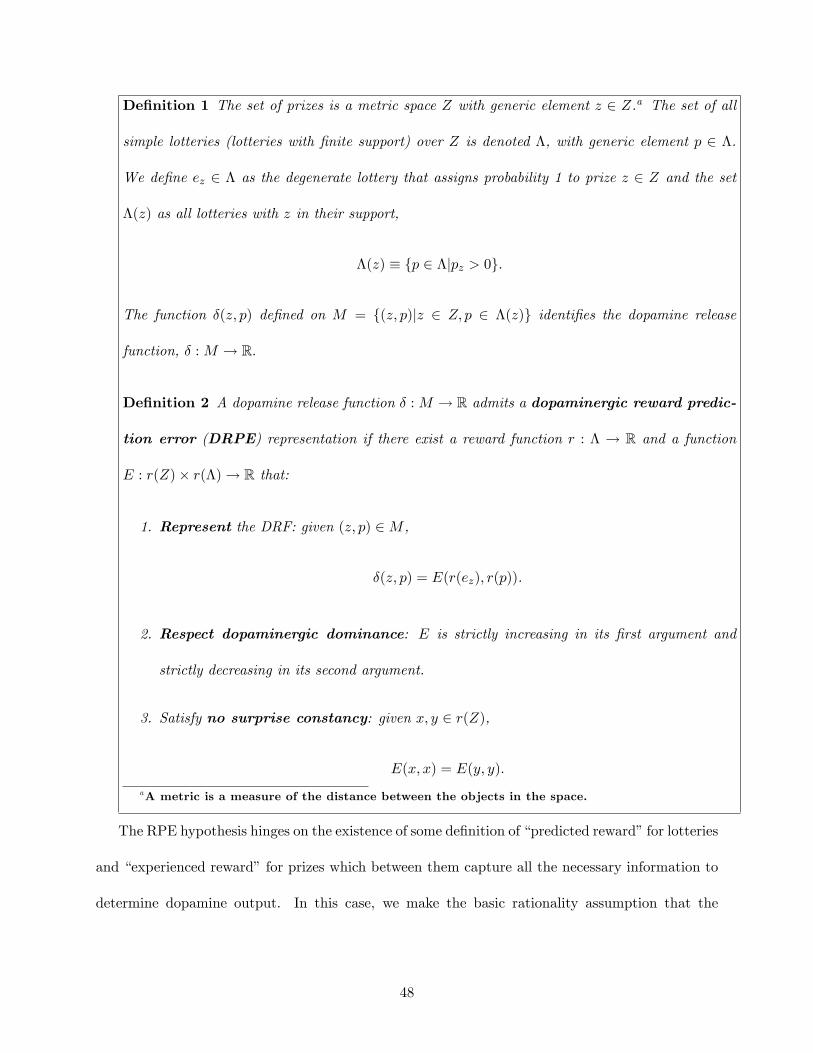
De�nition 1 The set of prizes is a metric space Z with generic element z 2 Z.a The set of all

simple lotteries (lotteries with �nite support) over Z is denoted �, with generic element p 2 �.

We de�ne ez 2 � as the degenerate lottery that assigns probability 1 to prize z 2 Z and the set

�(z) as all lotteries with z in their support,

�(z) � fp 2 �jpz > 0g:

The function �(z; p) de�ned on M = f(z; p)jz 2 Z; p 2 �(z)g identi�es the dopamine release

function, � :M ! R:

De�nition 2 A dopamine release function � :M ! R admits a dopaminergic reward predic-

tion error (DRPE) representation if there exist a reward function r : � ! R and a function

E : r(Z)� r(�)! R that:

1. Represent the DRF: given (z; p) 2M ,

�(z; p) = E(r(ez); r(p)).

2. Respect dopaminergic dominance: E is strictly increasing in its �rst argument and

strictly decreasing in its second argument.

3. Satisfy no surprise constancy: given x; y 2 r(Z),

E(x; x) = E(y; y):

aA metric is a measure of the distance between the objects in the space.

The RPE hypothesis hinges on the existence of some de�nition of �predicted reward�for lotteries

and �experienced reward�for prizes which between them capture all the necessary information to

determine dopamine output. In this case, we make the basic rationality assumption that the

48

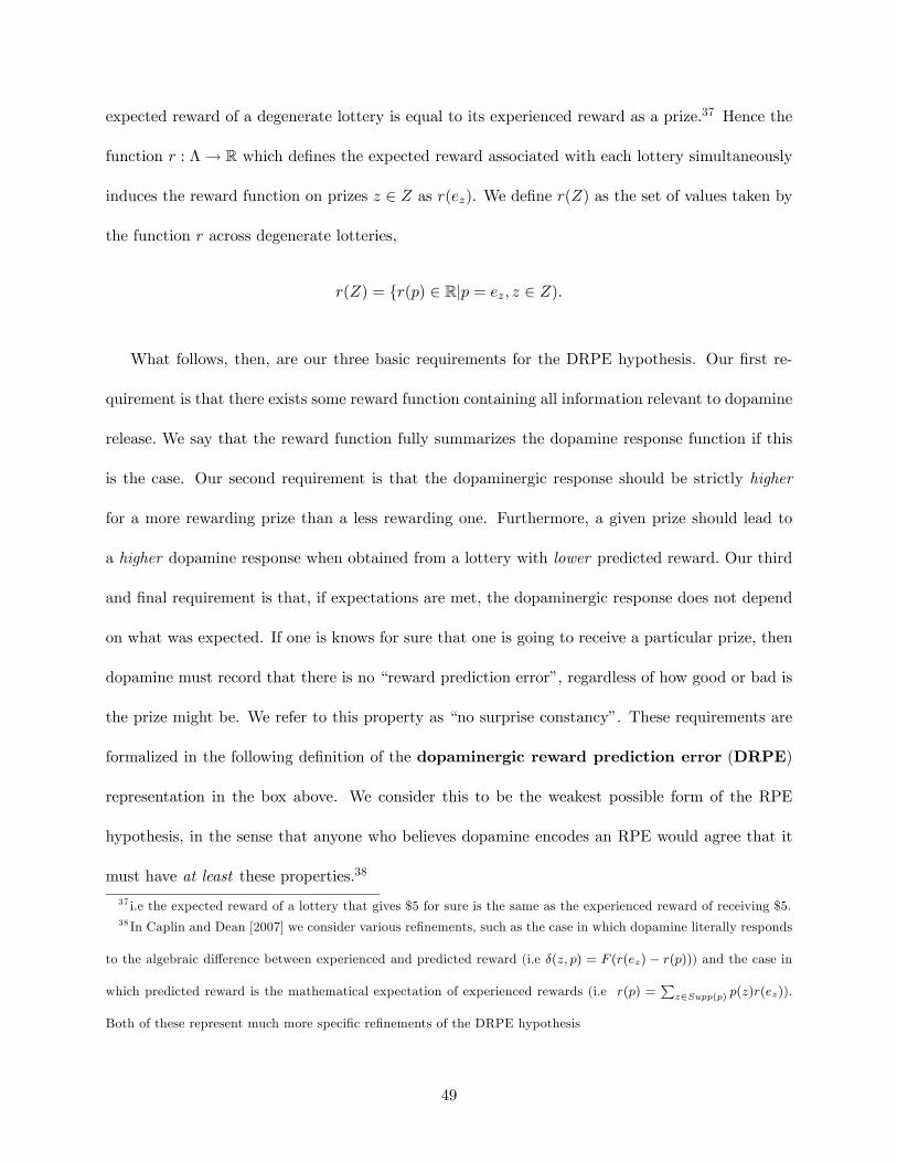
expected reward of a degenerate lottery is equal to its experienced reward as a prize.37 Hence the

function r : �! R which de�nes the expected reward associated with each lottery simultaneously

induces the reward function on prizes z 2 Z as r(ez). We de�ne r(Z) as the set of values taken by

the function r across degenerate lotteries,

r(Z) = fr(p) 2 Rjp = ez; z 2 Z):

What follows, then, are our three basic requirements for the DRPE hypothesis. Our �rst re-

quirement is that there exists some reward function containing all information relevant to dopamine

release. We say that the reward function fully summarizes the dopamine response function if this

is the case. Our second requirement is that the dopaminergic response should be strictly higher

for a more rewarding prize than a less rewarding one. Furthermore, a given prize should lead to

a higher dopamine response when obtained from a lottery with lower predicted reward. Our third

and �nal requirement is that, if expectations are met, the dopaminergic response does not depend

on what was expected. If one is knows for sure that one is going to receive a particular prize, then

dopamine must record that there is no �reward prediction error�, regardless of how good or bad is

the prize might be. We refer to this property as �no surprise constancy�. These requirements are

formalized in the following de�nition of the dopaminergic reward prediction error (DRPE)

representation in the box above. We consider this to be the weakest possible form of the RPE

hypothesis, in the sense that anyone who believes dopamine encodes an RPE would agree that it

must have at least these properties.38

37 i.e the expected reward of a lottery that gives $5 for sure is the same as the experienced reward of receiving $5.38 In Caplin and Dean [2007] we consider various re�nements, such as the case in which dopamine literally responds

to the algebraic di¤erence between experienced and predicted reward (i.e �(z; p) = F (r(ez) � r(p))) and the case in

which predicted reward is the mathematical expectation of experienced rewards (i.e r(p) =P

z2Supp(p) p(z)r(ez)).

Both of these represent much more speci�c re�nements of the DRPE hypothesis

49

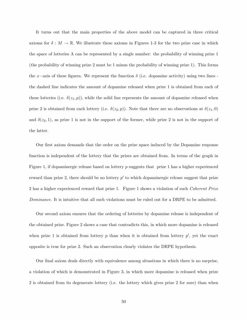
It turns out that the main properties of the above model can be captured in three critical

axioms for � : M ! R. We illustrate these axioms in Figures 1-3 for the two prize case in which

the space of lotteries � can be represented by a single number: the probability of winning prize 1

(the probability of winning prize 2 must be 1 minus the probability of winning prize 1). This forms

the x�axis of these �gures. We represent the function � (i.e. dopamine activity) using two lines -

the dashed line indicates the amount of dopamine released when prize 1 is obtained from each of

these lotteries (i.e. �(z1; p)), while the solid line represents the amount of dopamine released when

prize 2 is obtained from each lottery (i.e. �(z2; p)). Note that there are no observations at �(z1; 0)

and �(z2; 1), as prize 1 is not in the support of the former, while prize 2 is not in the support of

the latter.

Our �rst axiom demands that the order on the prize space induced by the Dopamine response

function is independent of the lottery that the prizes are obtained from. In terms of the graph in

Figure 1, if dopaminergic release based on lottery p suggests that prize 1 has a higher experienced

reward than prize 2, there should be no lottery p0 to which dopaminergic release suggest that prize

2 has a higher experienced reward that prize 1. Figure 1 shows a violation of such Coherent Prize

Dominance. It is intuitive that all such violations must be ruled out for a DRPE to be admitted.

Our second axiom ensures that the ordering of lotteries by dopamine release is independent of

the obtained prize. Figure 2 shows a case that contradicts this, in which more dopamine is released

when prize 1 is obtained from lottery p than when it is obtained from lottery p0, yet the exact

opposite is true for prize 2. Such an observation clearly violates the DRPE hypothesis.

Our �nal axiom deals directly with equivalence among situations in which there is no surprise,

a violation of which is demonstrated in Figure 3, in which more dopamine is released when prize

2 is obtained from its degenerate lottery (i.e. the lottery which gives prize 2 for sure) than when

50

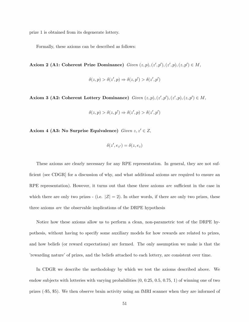
prize 1 is obtained from its degenerate lottery.

Formally, these axioms can be described as follows:

Axiom 2 (A1: Coherent Prize Dominance) Given (z; p); (z0; p0); (z0; p); (z; p0) 2M ,

�(z; p) > �(z0; p)) �(z; p0) > �(z0; p0)

Axiom 3 (A2: Coherent Lottery Dominance) Given (z; p); (z0; p0); (z0; p); (z; p0) 2M ,

�(z; p) > �(z; p0)) �(z0; p) > �(z0; p0)

Axiom 4 (A3: No Surprise Equivalence) Given z; z0 2 Z;

�(z0; ez0) = �(z; ez)

These axioms are clearly necessary for any RPE representation. In general, they are not suf-

�cient (see CDGR] for a discussion of why, and what additional axioms are required to ensure an

RPE representation). However, it turns out that these three axioms are su¢ cient in the case in

which there are only two prizes - (i.e. jZj = 2). In other words, if there are only two prizes, these

three axioms are the observable implications of the DRPE hypothesis

Notice how these axioms allow us to perform a clean, non-parametric test of the DRPE hy-

pothesis, without having to specify some auxiliary models for how rewards are related to prizes,

and how beliefs (or reward expectations) are formed. The only assumption we make is that the

�rewarding nature�of prizes, and the beliefs attached to each lottery, are consistent over time.

In CDGR we describe the methodology by which we test the axioms described above. We

endow subjects with lotteries with varying probabilities (0, 0.25, 0.5, 0.75, 1) of winning one of two

prizes (-$5, $5). We then observe brain activity using an fMRI scanner when they are informed of

51

what prize they have won for their lottery. We focus on the Nucleus Accumbens, an area within

the brain which is rich in dopamine output. While observing this area is clearly not the same

as observing dopamine, other authors [e.g. O�Doherty et al., 2003; 2004; Daw et al, 2006] claim

to have found RPE-like signals by collecting fMRI data from similar regions The noisy nature of

fMRI data does, however, force us to confront the issue of how the continuous and stochastic data

available to neuroscientists can be used to test axiomatic models. This is an area greatly in need of

systemization. CDGR take the obvious �rst step by treating each observation of fMRI activity when

some prize p is obtained from some lottery z as a noisy observation of actual dopamine activity from

that event. By repeated sampling of each possible event, we can used standard statistical methods

to test whether we can reject the null hypothesis that;for example, �(p; z) = �(q; w) against the

hypothesis that �(p; z) > �(q; w). It is these statistical tests to test the axioms that form the basis

of our theory.

5 Conclusion

To many non-economists, the bene�ts of using information on the underlying process of decision

making to help us build models of choice are obvious. Yet many people within economics remain

unconvinced by the its bene�ts. For the most part, I believe that this is because neuroeconomists

have taken up a tough, but extremely worthwhile challenge. Neuroeconomists have made signi�cant

strides in understanding how choices are instantiated in the brain, and over time this understanding

is likely to give rise to insights that are of direct relevance to economists. The speed at which

this happens is likely to be increased if neuroeconomists take on board some of the perceptive

critiques that have come from some economic theorists. In particular, if neuroeconomists want to

use neurological data in order to test economic models, then they need to explain exactly why they

52

are doing so, and what they expect to learn that a standard behavioral experiment could not tell

them.

Many of the arguments made here are not exclusive to the domain of neuroeconomics. The

question of when it is useful to �dig beneath the surface�of the question one is interested in to

understand the underlying process is one that pervades many areas of enquiry, including those

in comparative decision making. For example, is it useful for someone who is interested in the

properties of an ecosystem to begin by modelling the behavior of the plants and animals of those

that make up that ecosystem? Does a biologist interested in animal decision making need to know

the systems that bring about these decisions? Many of the arguments I make above could be

applied directly to these cases, and so my answer is, in general, a guarded �yes�.

Furthermore, the axiomatic method I lay out in section 3 has potential to be useful in many

�elds of study related to decision making. The key advantage of this approach comes about when-

ever models involve unobservable, or �latent�elements. For economists and neuroeconomists, such

variables occur all the time, but they turn up in many other �elds as well, including biology and psy-

chology. In all of these cases, axioms can o¤er a degree of precision and clarity that can compliment

existing methods.

Acknowledgements With thanks to Andrew Caplin and Paul Glimcher for training me in the

ways of neuroeconomics. Also to Juan Carillio, Phil Crowley, Jim Morrow and Philipp Sad-

owski for comments on the chapter.

53

6 Appendix

In this Appendix we provide a guide to the terms and symbols used in describing the RPE model

and its axiomatic basis:

Prize: One of the objects that a decision maker could potentially receive (e.g. amounts of

money, squirts of juice) when uncertainty is resolved.

Lottery: A probability distribution over prizes (e.g. 50% chance of winning $5, 50% chance of

losing $3).

Support: The set of prizes that one can potentially receive from a lottery (e.g. for the lottery

50% chance of winning $5, 50% chance of losing $3, the support is {$5, $3}).

Degenerate Lottery: A lottery with a 100% probability of winning one prize

2 : �is a member of�in set notation (e.g. x 2 X indicates that x is an element of the set X, or

�New York�2�American Cities")

R : The set of all real numbers

j: �such that·�For example f(z; p)jz 2 Z; p 2 �(z)g means any z and p such that z is an element

of Z and p is an element of �(z)

!: �mapping to�. Used to describe a function, so f : X ! Y indicates a function f which

associates with each element in set X a unique element in set Y

54

7 References

Bayer, H., and P. Glimcher, �Midbrain Dopamine Neurons Encode a Quantitative Reward Predic-

tion Error Signal,�Neuron, 47 (2005), 129�141.

Bayer, H., B. Lau, and P. Glimcher, �Statistics of Midbrain Dopamine Neuron Spike Trains in

the Awake Primate,�Journal of Neurophysiology, 98 (2007), 1428�1439.

Bernheim, D. (2009), �On the Potential of Neuroeconomics: A Sober (but Hopeful) Appraisal�,

American Economic Journal: Microeconomics 1 (2), 1-41.

B. Douglas Bernheim & Antonio Rangel, 2004. "Addiction and Cue-Triggered Decision Processes,"

American Economic Review, American Economic Association, vol. 94(5), pages 1558-1590, Decem-

ber.

Bossaerts, P. Ming Hsu and K. Preuscho¤, �The Neurobiological Foundations of Valuation

in Human Decision Making under Uncertainty,� in: Glimcher, P.W., Camerer, C.F., Fehr, E.,

and Poldrack, R.A. (eds.), 2008, Neuroeconomics: Decision Making and the Brain. New York:

Academic Press

Brocas, I., Carrillo, J. D. (2008). The brain as a hierarchical organization. American Economic

Review. Vol. 98(4), pp. 1312-1346.

Bryan, G. (2010, November). Ambiguity and insurance. Yale working paper.

Busemeyer, J.R., Townsend, J.T., 1993. Decision �eld theory: a dynamic cognition approach

to decision making. Psychological Review 100, 432�459.

Camerer, C., Loewenstein, G., and D. Prelec. �Neuroeconomics: Why economics needs brains,�

Scandinavian Journal of Economics, 2004, 106, 555-579

55

� 2005 "Neuroeconomics: How Neuroscience Can Inform Economics," Journal of Economic

Literature, American Economic Association, vol. 43(1), pages 9-64, March.

Caplin A. �Economic Theory and Psychological Data� in: The Foundations of Positive and

Normative Economics, by Andrew Caplin and Andrew Shotter (eds.). Oxford University Press.

2008.

Caplin, A. and Mark Dean, �Dopamine, Reward Prediction Error, and Economics,�Quarterly

Journal of Economics, 123:2 (2008), 663-702.

� , 2011. "Search, choice, and revealed preference," Theoretical Economics, Econometric Soci-

ety, vol. 6(1), January.

Caplin, A., M. Dean, and D. Martin (2011): �Search and Satis�cing,� American Economic

Review, in press.

Caplin. A, & Mark Dean & Paul W. Glimcher & Robb B. Rutledge, 2010. "Measuring Beliefs

and Rewards: A Neuroeconomic Approach," The Quarterly Journal of Economics, MIT Press, vol.

125(3), pages 923-960, August.

Daw, N., J. P. O�Doherty, P. Dayan, B. Seymour, and R. J. Dolan, �Polar Exploration: Cortical

Substrates for Exploratory Decisions in Humans,�Nature, 441 (2006),876�879.

Dominique J.-F. de Quervain, Urs Fischbacher, Valerie Treyer, Melanie Schellhammer, Ulrich

Schnyder, Alfred Buck, and Ernst Fehr. "The Neural Basis of Altruistic Punishment", Science 27

August 2004: 305 (5688), 1254-1258.

Echenique, F., S. Lee, and M. Shum. 2011. ìThe Money Pump as a Measure of Revealed

Preference Violations.îJournal of Political Economy, 119(6): 1201-1223

56

Fehr, E., U. Fischbacher and M. Kosfeld (2005). Neuroeconomic foundations of trust and social

preferences: initial evidence. American Economic Review, 95(2), 346-351.

Fehr, E A. Rangel. Neuroeconomic foundations of economic choice - Recent advances. Journal

of Economic Perspectives, 2011, 25(4):3-30.

Glimcher, P. "Foundations of Neuroeconomic Analysis" New York: Oxford University Press,

2010,

Glimcher P.W. (2011). Understanding dopamine and reinforcement learning: The dopamine

reward prediction error hypothesis. Proc Natl Acad Sci, 108 Suppl 3: 15647-1565

Glimcher, P.W., Camerer, C.F., Fehr, E., and Poldrack, R.A. (eds.), 2008, Neuroeconomics:

Decision Making and the Brain. New York: Academic Press,

Faruk Gul & Wolfgang Pesendorfer, 2006."Random Expected Utility," Econometrica, Econo-

metric Society, vol. 74(1), pages 121-146, 01.

� "The Case for Mindless Economics" [paper], in: The Foundations of Positive and Normative

Economics, by Andrew Caplin and Andrew Shotter (eds.). Oxford University Press. 2008.

T.A. Hare, C.F. Camerer, D.T. Knoep�e, J.P. O�Doherty, A. Rangel, Value computations in

ventral medial prefrontal cortex during charitable decision making incorporate input from regions

involved in social cognition. Journal of Neuroscience, 2010, 30:583-590.

T.A. Hare, C.F. Camerer, A. Rangel, Self-control in decision-making involves modulation of the

vmPFC valuation system. Science, 2009, 324:646-648.

T. A. Hare, W. Schultz, C. Camerer, J. O�Doherty, A. Rangel. Transformation of stimulus

value signals into motor commands during simple choice. PNAS, 2011, 108:18120-18125

57

Harrison, Glenn W., 2008. "Neuroeconomics: A Critical Reconsideration," Economics and

Philosophy, Cambridge University Press, vol. 24(03), pages 303-344, November.

Heeger DJ, Normalization of cell responses in cat striate cortex, Vis Neurosci, 9:181-198, 1992.

Heeger DJ, Modeling simple cell direction selectivity with normalized, half-squared, linear op-

erators, J Neurophysiol, 70:1885-1898, 1993.

Hsu, M., Bhatt, M., Adolphs, R., Tranel, D. & Camerer, C. F. 2005 Neural systems responding

to degrees of uncertainty in human decision-making. Science 310, 1680�1683.

Iyengar, S. S., & Lepper, M. (2000). When Choice is Demotivating: Can One Desire Too Much

of a Good Thing? Journal of Personality and Social Psychology, 79, 995-1006

Gardner, Eliot, and James David, �The Neurobiology of Chemical Addiction,� in Getting

Hooked: Rationality and Addiction, Jon Elster and Ole-Jorgen Skog, eds. (Cambridge, MA: Cam-

bridge University Press, 1999).

Johnson, Eric J.; Camerer, Colin; Sen, Sankar and Rymon, Talia. "Detecting Failures of Back-

ward Induction: Monitoring Information Search in Sequential Bargaining." Journal of Economic

Theory, 2002, 104(1), pp. 16-47

Kable, J.W., and Glimcher, P.W. (2007). The neural correlates of subjective value during

intertemporal choice. Nat Neuroscience. 10(12): 1625 - 1633.

Knoch D, Pascual-Leone A, Meyer K, Treyer V, Fehr E. 2006. Diminishing Reciprocal Fairness

by Disrupting the Right Prefrontal Cortex. Science 314:829-32

Kiyatkin, E. A., and A. Gratton, �Electrochemical Monitoring of Extracellular Dopamine in

Nucleus Accumbens of Rats Lever-Pressing for Food,�Brain Research, 652 (1994), 225�234.

58

Laibson, David (1997). "Golden Eggs and Hyperbolic Discounting". Quarterly Journal of

Economics 112 (2): 443�477

Levy, Ifat, Stephanie C. Lazzaro, Robb B. Rutledge, and Paul W. Glimcher. 2011. �Choice

from Non-Choice: Predicting Consumer Preferences from Blood Oxygenation Level-Dependent

Signals Obtained During Passive Viewing.�Journal of Neuroscience, 31(1): 118�25

Levy, I., Snell, J., Nelson, A.J., Rustichini, A., and Glimcher, P.W. (2010). Neural representa-

tion of subjective value under risk and ambiguity. Journal of Neurophysiology. 103(2):1036-47.

Li, J., S. M. McClure, B. King-Casas, and P. R. Montague, �Policy Adjustment In A Dynamic

Economic Game,�PlosONE, forthcoming, 2007.

Lucas, Robert (1976), "Econometric Policy Evaluation: A Critique", in Brunner, K.; Meltzer,

A., The Phillips Curve and Labor Markets, Carnegie-Rochester Conference Series on Public Policy,

1, New York: American Elsevier, pp. 19�46

Luce, R. D. (1959). Individual Choice Behavior: A Theoretical Analysis. New York: Wiley.

Marr D. (1982). "Vision. A Computational Investigation into the Human Representation and

Processing of Visual Information. W.H. Freeman and Company

Samuel M. McClure, David I. Laibson, George Loewenstein, and Jonathan D. Cohen "Separate

Neural Systems Value Immediate and Delayed Monetary Rewards" Science 15 October 2004: 306

(5695), 503-507

McFadden, D., (1973), �Conditional Logit Analysis of Qualitative Choice Behavior �in P. Zarem-

bka(ed), Frontiers in Econometrics Academic Press, New York 105-142

McItnosh, D. [1969] The Foundations of Human Society, U. Chicago Press, Chicago

59

Padoa-Schioppa C, Assad JA (2008). The representation of economic value in the orbitofrontal

cortex is invariant for changes of menu. Nat Neurosci. 11 (1): 95-10

Metcalfe, J., & Jacobs, W. J. (1996). A �hot-system/cool-system" view of memory under stress.

PTSD Research Quarterly, 7(2), 1-3.

Mirenowicz, J., and W. Schultz, �Importance of Unpredictability for Reward Responses in

Primate Dopamine Neurons,�Journal of Neurophysiololgy, 72(2)

(1994), 1024�1027.

Montague, P. R., and G. S. Berns, �Neural Economics and the Biological Substrates of Valua-

tion,�Neuron, 36 (2002), 265�284.

O�Doherty, J., P. Dayan, K. J. Friston, H. D. Critchley, and R. J. Dolan, �Temporal Di¤erence

Models Account and Reward-Related Learning in the Human

Brain,�Neuron, 38 (2003), 329�337.

O�Doherty, J., P. Dayan, J. Schultz, R. Deichmann, K. Friston, and R. J. Dolan, �Dissociable

Roles of Ventral and Dorsal Striatum in Instrumental Conditioning,�

Science, 304 (2004), 452�454.

Olds, J., and P. Milner, �Positive Reinforcement Produced by Electrical Stimulation of Septal

Area and Other Regions of Rat Brain,�Journal of Comparative and Physiological Psychology, 47

(1954), 419�427.

Preuscho¤ K, Bossaerts P, Quartz S (2006) Neural di¤erentiation of expected reward and risk

in human subcortical structures. Neuron 51:381�390

Ross, D. (2010). Neuroeconomics and economic methodology. In J. Davis and W. Hands, eds., Hand-

60

book of Economic Methodology. Cheltenham: Edward Elgar.

Rangel, A, C. Camerer, and R. Montague, A framework for studying the neurobiology of value-

based decision-making. Nature Reviews Neuroscience, 2008, 9:545-556

Rubinstein, A. "Lecture Notes in Microeconomic Theory: The Economic Agent" Princeton

University Press 2007

Rustichini, Aldo , Is there a Method of Neuroeconomics?" American Economic Review: Micro-

economics, (2009)

Samuelson, Paul A. (1938, February). nA Note on the Pure Theory of Consumer�s Behavior."

Economica 5, 61{71)

Schultz, Wolfram, Paul Apicella, and Tomas Ljungberg, �Responses of Monkey Dopamine Neu-

rons to Reward and Conditioned Stimuli during Successive Steps of Learning a Delayed Response

Task,�Journal of Neuroscience, 13 (1993), 900�913.

Schultz, Wolfram, Peter Dayan, and P. Read Montague, �A Neural Substrate of Prediction and

Reward,�Science, 275 (1997), 1593�1599.

Simon, Herbert. 1955. �A Behavioral Model of Rational Choice.�Quarterly Journal of Eco-

nomics, 69(1): 99-118

Smith, Alec, B. Douglas Bernheim, Colin Camerer, and Antonio Rangel. 2011. �Neural Activity

Reveals Preferences without Choices.�Unpublished manuscript

Sugrue LP, Corrado GS, Newsome WT (2005) Choosing the greater of two goods: neural

currencies for valuation and decision making. Nat Rev Neurosci 6:363�375.

Tom SM, Fox CR, Trepel C, Poldrack RA (2007) The neural basis of loss aversion in decision-

61

making under risk. Science 315:515�518.

E. Tricomi, A. Rangel, C.F. Camerer, J.P. O�Doherty, Neural evidence for inequality-averse

social preferences. Nature, 2010, 463:1089-1091.

Wallis, J.D. and Miller, E.K. (2003) Neuronal activity in the primate dorsolateral and orbital

prefrontal cortex during performance of a reward preference task. European Journal of Neuro-

science. 18:2069-2081

Wunderlich, K. , A. Rangel, J.P. O�Doherty, Neural computations underlying action-based

decision making in the human brain. PNAS, 2009, 106(40):17199:17204.

62

Dopam

ine Release

p P’

Figure 1

A violation of A1: when received from lottery p, prize 1 leads to higher dopamine release than does prize 2 indicating that prize 1 has higher experienced reward. This order is reversed when the prizes are realized from lottery p’, suggesting prize 2 has higher experienced reward. Thus a

DRPE representation is impossible.

p p’

Dopam

ine Release

Figure 2

A violation of A2: Looking at prize 1, more dopamine is released when this prize is obtained from p’ than when obtained from p, suggesting that p has a higher predicted reward than p’.

The reverse is true for prize2, making a DRPE representation impossible

Dopam

ine Release

Figure 3

A violation of A3: the dopamine released when prize 1 is obtained from its sure thing lottery is higher that that when prize 2 is obtained from its sure thing lottery.