chapter 8. calculation of pfd using fta · fault tree analysis (fta) is a widely used and popular...

Chapter 8.Calculation of PFD using FTA

Mary Ann Lundteigen Marvin Rausand

RAMS GroupDepartment of Mechanical and Industrial Engineering

NTNU

(Version 0.1)

Lundteigen& Rausand Chapter 8.Calculation of PFD using FTA (Version 0.1) 1 / 34

Introduction

Learning Objectives

The main learning objectives associated with these slides are to:I Present and discuss the application of fault tree analysis for calculating

the PFD• First, with basis in the SIS text book• Second, with basis in a referenced paper (“procedure”)1

I Highlight some of the challenges related to using (some) commercialso�ware

The slides include topics from Chapter 8 in Reliability of Safety-CriticalSystems: Theory and Applications. DOI:10.1002/9781118776353.

1Reliability assessment of safety instrumented systems in the oil and gas industry: Apractical approach and a case study by Lundteigen, M.A. and Rausand, M., The InternationalJournal of Reliability, �ality and Safety Engineering (IJRQSE) Vol. 16 (2009),see http://dx.doi.org/10.1142/S0218539309003356


http://dx.doi.org/10.1142/S0218539309003356

Introduction

Outline of Presentation

1 Introduction

2 FTA Basics

3 PFD basics

4 Beyond SIS Textbook

5 Procedure

6 Reflections


FTA Basics

Application and Characteristics

Fault tree analysis (FTA) is a widely used and popular method for reliabilityanalysis, and is suggested in IEC 61508 as a relevant approach for reliabilityanalysis of SIS.

A more detailed introduction to the characteristics of FTA is found inchapter 5 of the SIS textbook


FTA Basics

Fault Tree Analysis (FTA) - for SIS

Main elements of a fault tree:

I TOP event

I Gates (and, or, koon).

I Basic events

I Transfer symbols (triangles)

Typical TOP events for a SIS:

I TOP1: The SIF cannot beperformed (e.g., fail to stopflow upon demand)

I TOP2: The SIF is activatedspuriously (e.g., the stopsflow when not demanded)

Fail to stop flow

Both pressuresensors fail

Pressure sensor #1 fails

PS1


PS2

PLC fails

PLC

Valve fails

V


FTA Basics

Fault tree analysis (FTA) - for SIS

A fault tree may be split into several sub-trees (sub-trees shown for sensor system,without and with CCFs included):

SIF fails-to-functionon demand

Sensor subsystem fails-to-function

on demand

Logic solver subsystem fails-to-function

on demand

Final element subsystem fails-to-function

on demand

FELSS


on demand

PT 1 fails-to-function

on demand

PT 1 PT 2 PT 3


on demand


on demand

S

or


on demand


on demand

PT 1 PT 2 PT 3

CCF


on demand

IndependentPT failureson demand

Common-causefailure

on demand


on demand

S


FTA Basics

Fault tree for koon systems

A SIS is o�en split into subsystems, where each is voted koon. Each subsystem canbe studied separately using the upper bound approximation

Consider a koon system:

I The system fails if (n − k + 1) components fail.

I This implies that the minimal cutsets are of order (n − k + 1).

I The number of minimal cut sets are κ =(

nn−k+1

).

Example

The number of minimal cutsets in a 2oo4 system is:(43

)=

4!(4 − 3)!3!

=4 · 3 · 2 · 11 · 3 · 2 · 1

= 4


FTA Basics

FTA versus RBD

When should we use FTA and when should we use a reliability block diagram(RBD)?

I With AND and OR gates, a FT can always be transferred to an RBD and visaverse.

I Some prefer failure oriented modeling, rather than success oriented.

I A RBD o�en aims for a structure that resembles the physical structure of thesystem. Many of the simplified formulas developed for RBDs assume that thesystem may be split into a series structure of subsystems, but this is notalways possible for more complex systems.

I With FTA, we base the calculations on the minimal cutsets, and we do notneed be concerned about how we model as long as we have algorithms toextract these.


PFD basics

Approach for calculating PFD

In FTA we may calculate the average PFD by:

I First finding the failure function Q0 (t)for the top event and then calculate thePFD average by:

PFDavg =1τ

∫ τ

0Q0 (t)dt

I or, use the upper bound approximation using the minimal cut sets (MCSs)2.

PFDavg ≤ 1 −κ∏

j=0

(1 − Q̌j,avg )

I The la�er approach is o�en preferred, but how shall the Q̌j,avg be calculated?

2Minimal cut sets: the sets that contain the least combinations of component failures that result in the TOP event


PFD basics

Calculation problem for koon system

Consider first the koon system with identical and independent components:

I The main approach for calculating the probability of a minimal cutsetoccuring in a time interval t, here referred to as Q̌j (t), j = 1 . . .κ, whereκ =

(n

n−k+1

)is:

Q̌j (t) =n−k+1∏i=1

qi (t)

where qi (t) is the probability that component i fails in the time interval.


PFD basics

Calculation problem for koon system

Most so�ware programs calculate the PFD at the basic event level rather than at thelevel of the minimal cutset.

Q̌j,avg =

n−k+1∏i=1

qi,avg

where qi,avg =λDU τ2 . This means that:

Q̌j,avg =

(λDUτ2

)n−k+1For comparison, the simplified formulas for a koon system has previously beenfound as:

PFD1oo(n−k+1)avg =

(λDUτ )n−k+1

n − k + 2

This is not conservative since n − k + 2 < 2n−k+1. Check for yourself for e.g. a1oo2system.


PFD basics

Correction factor for minimal cut sets

The following correction factor (CF) may be used in relation to eachminimial cut set, if the average failure probability in (0,τ ) is calculated atthe basic event level:

CF =2n−k+1

n − k + 2


Beyond SIS Textbook

Minimal Cut Sets with Non-Identical Components

The slides beyond this point are not covered by the SIStextbook, but by the referenced paper.


Beyond SIS Textbook

Non-identical, but independent components

Consider a minimal cutset j with mj3 independent and non-identical components with test

interval τ . The PFDmcs, j of this minimal cut is

PFDmcs, j =1τ

∫ τ

0

mj∏i=1

(1 − e−λDU, j, i ·t

)dt

/1τ

∫ τ

0

mj∏i=1

(λDU, j, i · t

)dt =

(∏mji=1 λDU, j, i

)· τmj

mj + 1

=

(λ̄DU, j · τ

)mj

mj + 1

where

λ̄DU, j = *,

mj∏i=1

λDU, j, i+-

1mj

is the geometric mean of the mj DU-failure rates λDU, j,1, λDU, j,2, . . . , λDU, j,mj .

3Assuming that there is a list of MCSs can have di�erent dimensions


Beyond SIS Textbook

Example

For a minimal cut j of two independent components with failure rates λDU, j,1 and λDU, j,2,the average PFDMCj is:

PFDMCj /λDU, j,1 · λDU, j,2 · τ

2

3

This is 3/4 of the non-conservative approximation (λDU, j,1 · λDU, j,2 · τ 2/4). In general (for a1oomj voted configuration), the correction factor is:

2mj

mj + 1


Beyond SIS Textbook

Modeling CCFs

Components are not always failing independent of each other, and we need toinclude the contribution from common cause failures (CCFs).

Z Common cause failure (CCF): A dependent failure in which two or morecomponent fault states exist simultaneously or within a short time interval, and area direct result of a shared cause.

It is common to use the standard beta factor model in relation to fault tree analysis.

I Some minimal cutsets may constitute identical components

I More common is perhaps that they constitute some identical and somenon-identical components

It is therefore not always straigt forward to find or determine representative valuesof beta.


Beyond SIS Textbook

Model CCFs as basic events into the FT

Common cause failures(CCFs) may be includedin a fault tree by:

I Explicit modeling

I Implicit modeling

In this way, the MCSswill constitute indepen-dent as well as CCFevents.

Fail to stop flow

Both pressuresensors fail


PS1


PS2

PLC fails

PLC

Valve fails

V

Both failindependently

Both faildue to CCF

CCF

Both faildue to CCF

HE Vibr Calibr Plugg

Explicitmodeling

Implicit modeling


Beyond SIS Textbook

Post-Processing of CCFs

There are some arguments to why CCFs should be added in the post-processing ofminimal cut sets, and not added as CCF basic events in the fault tree.

I In many cases, the minimal cut sets include basic events, with potentialdependencies, from di�erent sections of the FT. It is not obvious where andhow CCFs should be added as basic events in the fault tree.

I Within the same minimal cut set, there may be some basic events that aredependent while others are independent. We may refer to this as minimal cutsets having di�erent internal dependencies. This can be easier to evaluate,once the minimal cut sets have been derived.

Remark: A koon gate (with n > 1, k > 1) in a fault tree generates(

nn−k+1

)minimal

cut sets, but CCFs cannot be added to each of these using the assumption that all ncomponents fail in a koon system in case of a CCF.


Beyond SIS Textbook

Internal Dependencies

Illustration of the situation where a minimalcutset (MCS) has di�erent internal dependen-cies:I This MCS number has order 5 ({C1, C2,

C3, C4, C5}) when consideringindependent failures only

I For CCFs, it s assumed that there aretwo sets (“common cause componentgroups, CCCG) of internaldependencies: CCCG1 for {C1,C2} andCCCG2 for {C4,C5}.

C1

C3

C2

C4

C5

CCF1

CCF2

CCCG1

CCCG2


Procedure

Procedure (based on article)

A procedure has been proposed for deriving at formulas for PFDavg . Themost important a�ributes of the approach are:I Simplified formulas are used to calculate PFDavg at the minimal cut set

(MCS) levelI The existence of dependencies, including common cause component

groups, are investigated a�er the MCSs have been generated, and thecontribution of CCFs is added to each minimal cut set using thestandard beta factor model

Note that steps 5-8 are covered here, and reference is made to thereferenced paper about the content of the other steps.


Procedure

Terminology

The following terms are used:I Common cause component group (CCCG): A collection of basic events

in a MCS where there exists a shared dependency. The same MCS mayhave more than one CCCG.


Procedure

Procedure steps

Fault tree constructionStep 3

Step 4 Identification and verification of MCSs

Step 2 TOP event definition

Step 1 System familiarization (of the SIF)

Step 5 Identification of CCCGs (for each MCS)

Step 6 Determine β for each CCCG

Step 7 Determine PFD for each MCS

Step 8 Calculate PFD of the function (SIF)

Note: Only the steps colored red (steps 5-8) are covered in the following slides.


Procedure

Step 5: Identification of CCCGs

Step 5 concerns the identification of the CCCFs for each MCSj .

I Look for potential coupling factors among components in the MCS, andplace components that share a coupling factor in the same CCCG.

I For each CCCFi in MCSj , define a CCF-event CCFi.

I Determine a value for a beta factor for each CCFi, by using data sourses,checklists, or expert judgment. In case of expert judgments, it is important toidentify possible root causes for the coupling factors, and evaluate how likelythey are or have been to occur.

O�en and in practice, only one CCCG is defined for each MCS since it may bedi�icult to support each CCCG by separate CCF data. Several guidelines andstandards include checklists for root causes and coupling factors.


Procedure

Step 6: Determine β for each CCCG

Step 6 aims to determine the value of βi for each CCCGi, i = 1 . . . k. Applicableapproaches are::

I Checklists

I Expert judgments

I Estimation

Expert judgments is for example used in the OLF 070 guideline, whereas checklistsmay be found in IEC 61508, part 6, Unified Partial Method (UPM), and in an articleby Humphreys, R. A. (1987). The la�er approach may need to be calibrated in lightof current state of the art technology.


Procedure

Step 7: Determine PFD for each MCS

Step 7 is used to calculate the PFDavg for each MCSj . The PFDMCj is influenced by:

I The order mj of the minimal cut.

I Whether or not the components of the minimal cut are identical .

I Whether or not the components of the minimal cut are dependent .

I Whether or not the components of the minimal cut are tested simultaneously .

Three alternatives have been introduced:

I Alternative 1: Identical and independent.

I Alternative 2: Identical and dependent, with one CCCG.

I Alternative 3: Non-identical and dependent, with one CCCG.

I Alternative 4: More complex, with more than one CCCG.


Procedure


Alternative 1: Independent components with failure ratesλDU, j,1, λDU, j,2, . . . , λDU, j,mj :

I We may then use the formulas:

PFDMCj =1τ

∫ τ

0

mj∏i=1

(1 − exp(−λDU, j, i · t

)dt

/1τ

∫ τ

0

mj∏i=1

(λDU, j, i · t

)dt =

(∏mji=1 λDU, j, i

)· τmj

mj + 1

=

(λ̄DU, j · τ

)mj

mj + 1

where

λ̄DU, j = *,

mj∏i=1

λDU, j, i+-

1mj


Procedure


Alternative 2: Identical and dependent components:

I Consider a minimal cut with mj identical and dependent components withDU failure rate λDU, j and beta factor βj

I Assume that all the components of the minimal cut are tested simultaneouslywith test interval τ

The PFD for this structure, PFDMCj , then becomes :

PFDMCj /

((1 − βj )λDU, j · τ

)mj

mj + 1+βjλDU, j · τ

2


Procedure


Alternative 3: Non-identical and dependent components:

I Example: A temperature transmi�er and a pressure transmi�er, located in thesame area, can be vulnerable to vibration

I Problem: What β should we choose?

• Geometric mean: Ok, as long as the failure rates are not too di�erent inmagnitude

• If they are, the CCF rate may be greater than the lowest failure rate ofthe components being considered4

• Instead, we choose beta as a fraction of the lowest component failurerate

4Which is unrealistic when we assume the standard beta factor model


Procedure


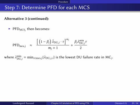
Alternative 3 (continued):

I PFDMCSj then becomes:

PFDmcs, j ≈

[ (1 − βj

)λ̄DU, j · τ

]mj

mj + 1+βjλ

minDU, jτ

2

where λminDU, j = mini∈mcs, j{λDU, j, i} is the lowest DU failure rate in MCj .


Procedure


Alternative 4: More complex MCSs (i.e., with more than one CCCG per MCS)

I A MCS may have more than one CCCG

I In the illustration below, the MCS may have order 4, 5, and 6

1

2

C1

C2

3

4

5

6

CG1

CG2


Procedure


Alternative 4 (continued):

I It is usually su�icient to calculate the PFD for the (virtual) cut set with thelowest order

I In the illustration on the previous frame, this is for {1, 2,C1,C2}

We then get (the index j has been omi�ed):

PFD(1)MC ≈

(λ(I )1 λ(I )2 β1β2λ

min,1DU λmin,2

DU

)τ 4

5

The PFD for the MCS, considering all ‘virtual cuts’ is:

PFDMCj ≈ 1 −∏

All“virtual′′cuts k

(1 − PFD(k)

MCj

)


Procedure

Step 8: Determine PFD of the SIF

The formula for calculating the PFD of the safety instrumented function (SIF),taking all the MCSs into account, is also based on the upper bound approximation:

PFDSIF / 1 −m∏j=1

(1 − PFDMCj

)


Procedure

Example application

The application of the procedure is demonstrated for a workover control system inthe referenced article (Lundteigen and Rausand, 2009).


Reflections

Pros/Cons

Pros:

I Using MCS as basis for modeling CCFs may be advantageous where the faulttrees are very large and where components, with potential dependencies, mayend up in very di�erent sections of the tree.

I The conservative approximation formulas are already well known byreliability analysts

Cons:

I Some more manual e�ort is needed (but this e�ort may be worth while takingto be�er understand the system)

I Care must be taken when using koon gates in FT, to avoid that thecontribution from CCFs are not added more than once.


chapter 8. calculation of pfd using fta · fault tree analysis (fta) is a widely used and popular...

Documents