chapter 8 matrices 2017 version 1 - paul weiser -...

Module 1: Matrices

of 38

Further Mathematics 2017 Module 1: Matrices (Chapter 8) Extract from Study Design Key knowledge

• the order of a matrix, types of matrices (row, column, square, diagonal, symmetric, triangular, zero, binary, permutation and identity), the transpose of a matrix, elementary matrix operations (sum, difference, multiplication of a scalar, product and power) • the inverse of a matrix and the condition for a matrix to have an inverse, including determinant • communication and dominance matrices and their application • the use of matrices to represent and solve a system of linear equations • transition diagrams and transition matrices and regular transition matrices and their identification. Key skills

• use the matrix recurrence relation: S0 = initial state matrix, Sn+1 = TSn to generate a sequence of state matrices, including an informal identification of the equilibrium or steady state matrix in the case of regular state matrices • construct a transition matrix from a transition diagram or a written description and vice versa • construct a transition matrix to model the transitions in a population with an equilibrium state • use the matrix recurrence relation S0 = initial state matrix, Sn+1 = TSn + B to extend the modelling to populations that include culling and restocking.

Chapter Sections Questions to be completed

8.2 Matrix representation 1, 2, 3, 4, 5, 6, 11, 12, 13, 14, 15 8.3 Addition, subtraction and scalar operations with matrices 3, 4, 7, 8, 9, 11, 13, 14c, 16, 17, 18

8.4 Multiplying matrices 2, 4, 5, 7, 8, 10, 13, 14, 16, 18,19 8.5 Multiplicative inverse and solving matrix equations 2, 4, 6, 7, 8, 11, 15, 16, 17, 18

8.6 Dominance and communication matrices 1, 2, 3, 5, 6, 7, 8, 10, 11, 13, 15, 17, 18 8.7 Application of matrices to simultaneous equations 2, 4, 5, 7cd, 8ce, 11, 13, 14, 15, 17

8.8 Transition matrices 1, 3, 5, 6, 8, 9, 11, 13, 15, 16, 18, 19, 22, 23

More resources available at http://drweiser.weebly.com/modules-‐2017

Module 1: Matrices

of 38

Table of ContentsEXTRACT FROM STUDY DESIGN .................................. 1 KEY KNOWLEDGE ....................................................... 1 KEY SKILLS ................................................................ 1

TABLE OF CONTENTS .......................................... 2

8.2 MATRIX REPRESENTATION ............................ 3

WHAT IS A MATRIX? ............................................... 3 TYPES OF MATRICES ................................................ 3 ROW MATRIX ............................................................ 3 COLUMN MATRIX ................................................... 3 THE TRANSPOSE OF A MATRIX: SWITCHING ROWS AND COLUMNS: ................................................................ 3 Example: Transpose of a matrix ............................ 4 SQUARE MATRIX ....................................................... 5 DIAGONAL MATRIX ..................................................... 5 ZERO MATRIX ............................................................ 5 SYMMETRICAL MATRIX ................................................ 5 TRIANGULAR MATRIX .................................................. 5 BINARY MATRIX ......................................................... 5 Worked Example 1 ................................................ 6 USING MATRICES TO STORE DATA ............................... 6 Worked Example 2 ................................................ 7

8.3 ADDITION, SUBTRACTION AND SCALAR OPERATIONS WITH MATRICES ............................ 8

ADDITION AND SUBTRACTION .................................... 8 Worked Example 3 ................................................ 8 SCALAR MULTIPLICATION .......................................... 8 Worked Example 4 ................................................ 9 MATRIX OPERATIONS ON THE CAS CALCULATOR ............. 9 PROPERTIES OF ADDITION OF MATRICES ..................... 10 SIMPLE MATRIX EQUATIONS .................................... 10 Worked Example 5 .............................................. 10 Worked Example 6 .............................................. 11

8.4 MULTIPLYING MATRICES ............................ 12

THE MULTIPLICATION RULE ..................................... 12 Worked Example 7 .............................................. 13 THE IDENTITY MATRIX ............................................ 14 THE SUMMATION MATRIX ...................................... 15 EXAMPLE USING MATRIX MULTIPLICATION TO SUM ROWS AND COLUMNS OF A MATRIX. ..................................... 15 PERMUTATION MATRIX .......................................... 16 Worked Example 8 .............................................. 16 PROPERTIES OF MULTIPLICATION OF MATRICES ............ 17 Worked Example 9 .............................................. 17 Worked Example 10 ............................................ 18

8.5 MULTIPLICATIVE INVERSE AND SOLVING MATRIX EQUATIONS ........................................ 19 FINDING THE INVERSE OF A SQUARE 𝟐×𝟐 MATRIX ....... 19 Worked Example 11 ............................................ 20 SINGULAR MATRICES ............................................. 20 Worked Example 12 ............................................ 20 FURTHER MATRIX EQUATIONS ................................. 21 WORKED EXAMPLE 13 ............................................. 21

8.6 DOMINANCE AND COMMUNICATION MATRICES ........................................................ 22

REACHABILITY ...................................................... 22 MATRIX REPRESENTATION ...................................... 22 Worked example 14 ............................................ 23 DOMINANCE ........................................................ 24 Worked Example 15 ............................................ 25 COMMUNICATION ................................................ 25 Worked Example 16 ............................................ 26

8.7 APPLICATION OF MATRICES TO SIMULTANEOUS EQUATIONS ............................ 27

Worked Example 17(a) ........................................ 27 Worked Example 17(b) ........................................ 28 DEPENDENT SYSTEMS OF EQUATIONS ........................ 29 INCONSISTENT SYSTEMS OF EQUATIONS ..................... 29 Worked Example 18 ............................................ 29 Worked Example 19 ............................................ 30

8.8 TRANSITION MATRICES ............................... 31

POWERS OF MATRICES ........................................... 31 Worked Example 20 ............................................ 31 MARKOV SYSTEMS AND TRANSITION MATRICES ........... 32 Worked Example 21 ............................................ 32 DISTRIBUTION VECTOR AND POWERS OF THE TRANSITION MATRIX .............................................................. 33 APPLICATIONS TO MARKETING .................................... 33 Worked Example 22 ............................................ 34 NEW STATE MATRIX WITH CULLING AND RESTOCKING ... 35 Worked Example 23 ............................................ 35 Worked Example 24 ............................................ 36 STEADY STATE ...................................................... 37 APPLICATIONS TO WEATHER ...................................... 37 Worked Example 25 ............................................ 38

Module 1: Matrices

of 38

8.2 Matrix representation What is a Matrix?

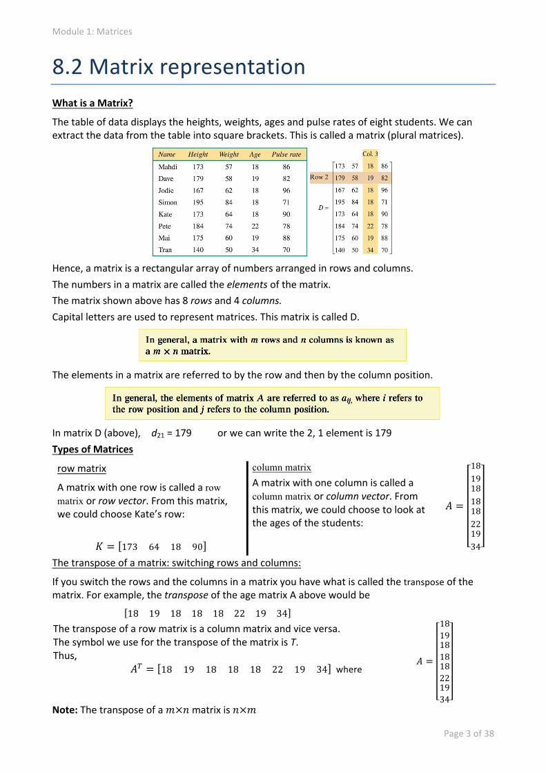
The table of data displays the heights, weights, ages and pulse rates of eight students. We can extract the data from the table into square brackets. This is called a matrix (plural matrices).

Hence, a matrix is a rectangular array of numbers arranged in rows and columns. The numbers in a matrix are called the elements of the matrix. The matrix shown above has 8 rows and 4 columns. Capital letters are used to represent matrices. This matrix is called D.

The elements in a matrix are referred to by the row and then by the column position.

In matrix D (above), d21 = 179 or we can write the 2, 1 element is 179 Types of Matrices

row matrix

A matrix with one row is called a row matrix or row vector. From this matrix, we could choose Kate’s row:

𝐾 = 173 64 18 90

column matrix A matrix with one column is called a column matrix or column vector. From this matrix, we could choose to look at the ages of the students:

𝐴 =

1819181818221934

The transpose of a matrix: switching rows and columns:

If you switch the rows and the columns in a matrix you have what is called the transpose of the matrix. For example, the transpose of the age matrix A above would be

Note: The transpose of a 𝑚×𝑛 matrix is 𝑛×𝑚

18 19 18 18 18 22 19 34 The transpose of a row matrix is a column matrix and vice versa. The symbol we use for the transpose of the matrix is T. Thus,

𝐴2 = 18 19 18 18 18 22 19 34 where

𝐴 =

1819181818221934

Module 1: Matrices

of 38

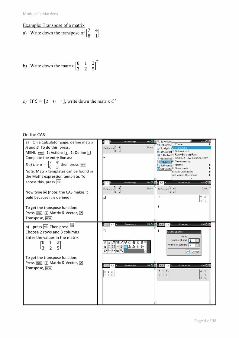
Example: Transpose of a matrix a) Write down the transpose of 7 4

8 1

b) Write down the matrix 0 1 23 2 5

2

c) If 𝐶 = 2 0 1 , write down the matrix 𝐶2 On the CAS a) On a Calculator page, define matrix A and B. To do this, press: MENU b, 1: Actions 1, 1: Define 1 Complete the entry line as:

𝐷𝑒𝑓𝑖𝑛𝑒 𝑎 = 7 48 1 then press ·

Note: Matrix templates can be found in the Maths expression template. To access this, press t Now type A (note: the CAS makes it bold because it is defined) To get the transpose function: Press b, 7 Matrix & Vector, 2 Transpose, ·

b) press t Then press Choose 2 rows and 3 columns Enter the values in the matrix

0 1 23 2 5

To get the transpose function: Press b, 7 Matrix & Vector, 2 Transpose, ·

Module 1: Matrices

of 38

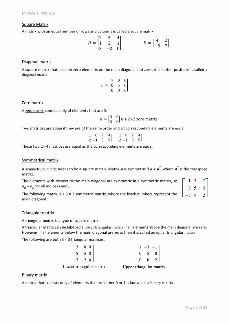
Square Matrix A matrix with an equal number of rows and columns is called a square matrix

𝐷 =2 5 41 2 13 −2 0

𝐸 = 4 2−5 7

Diagonal matrix

A square matrix that has non-‐zero elements on the main diagonal and zeros in all other positions is called a diagonal matrix

𝐹 =7 0 00 5 00 0 6

Zero matrix

A zero matrix consists only of elements that are 0.

𝐺 = 0 00 0 is a 2×2 zero matrix

Two matrices are equal if they are of the same order and all corresponding elements are equal.

12 0 −1

2 43 5 = 1

2 0 −1

2 43 5

These two 2´4 matrices are equal as the corresponding elements are equal.

Symmetrical matrix

A symmetrical matrix needs to be a square matrix. Matrix A is symmetric if A = AT, where AT is the transpose matrix.

The elements with respect to the main diagonal are symmetric in a symmetric matrix, so aij = aji for all indices i and j.

The following matrix is a 3 × 3 symmetric matrix, where the black numbers represent the main diagonal

Triangular matrix

A triangular matrix is a type of square matrix. A triangular matrix can be labelled a lower triangular matrix if all elements above the main diagonal are zero. However, if all elements below the main diagonal are zero, then it is called an upper triangular matrix.

The following are both 3 × 3 triangular matrices.

Binary matrix

A matrix that consists only of elements that are either 0 or 1 is known as a binary matrix.

Module 1: Matrices

of 38

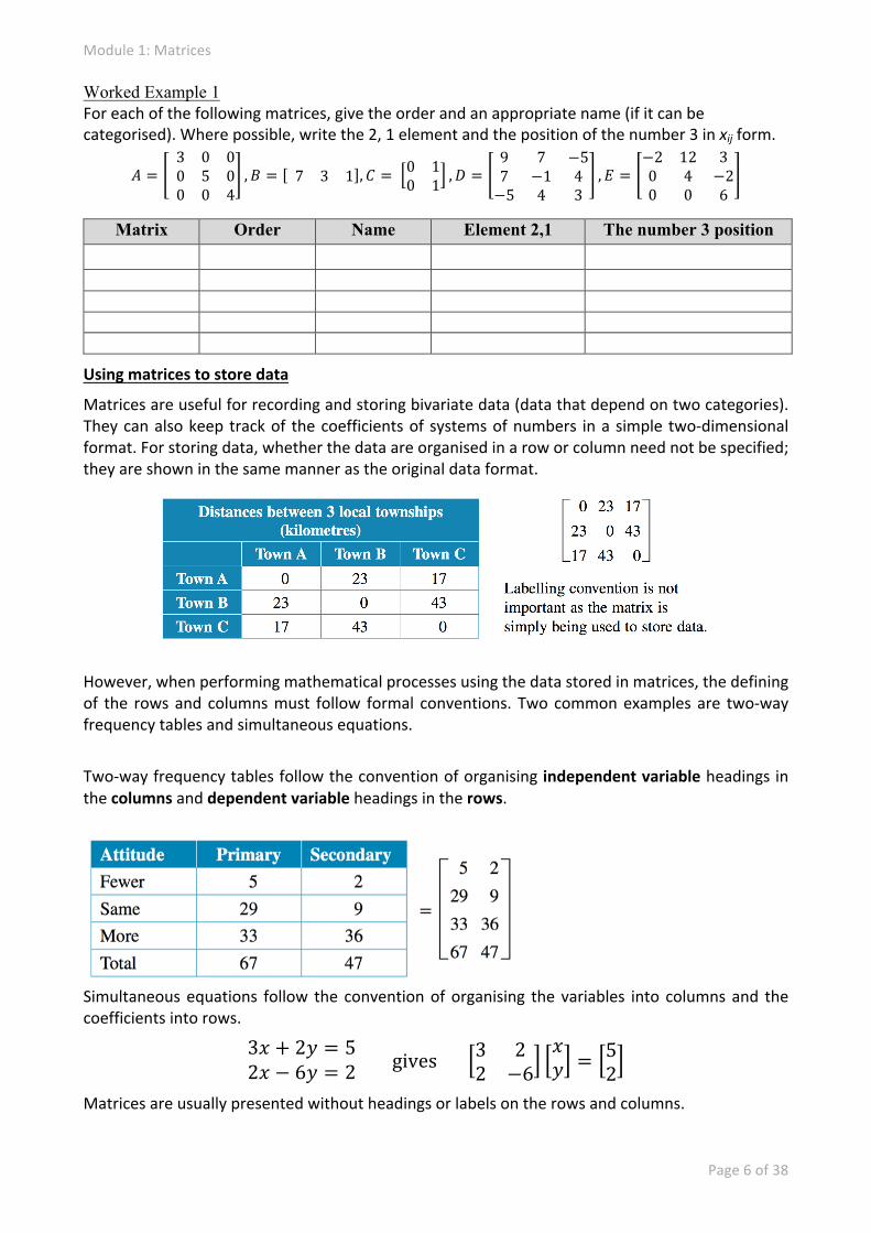
Worked Example 1 For each of the following matrices, give the order and an appropriate name (if it can be categorised). Where possible, write the 2, 1 element and the position of the number 3 in xij form.

𝐴 = 3 0 00 5 00 0 4

, 𝐵 = 7 3 1 , 𝐶 = 0 10 1 , 𝐷 =

9 7 −57 −1 4−5 4 3

, 𝐸 =−2 12 30 4 −20 0 6

Matrix Order Name Element 2,1 The number 3 position

Using matrices to store data

Matrices are useful for recording and storing bivariate data (data that depend on two categories). They can also keep track of the coefficients of systems of numbers in a simple two-‐dimensional format. For storing data, whether the data are organised in a row or column need not be specified; they are shown in the same manner as the original data format.

However, when performing mathematical processes using the data stored in matrices, the defining of the rows and columns must follow formal conventions. Two common examples are two-‐way frequency tables and simultaneous equations.

Two-‐way frequency tables follow the convention of organising independent variable headings in the columns and dependent variable headings in the rows.

Simultaneous equations follow the convention of organising the variables into columns and the coefficients into rows.

3𝑥 + 2𝑦 = 52𝑥 − 6𝑦 = 2 gives

3 22 −6

𝑥𝑦 = 5

2

Matrices are usually presented without headings or labels on the rows and columns.

Module 1: Matrices

of 38

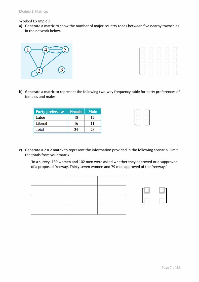
Worked Example 2 a) Generate a matrix to show the number of major country roads between five nearby townships

in the network below.

��

��

��

��

��

� � � � ��

b) Generate a matrix to represent the following two-‐way frequency table for party preferences of females and males.

� ��

c) Generate a 2 × 2 matrix to represent the information provided in the following scenario. Omit the totals from your matrix.

‘In a survey, 139 women and 102 men were asked whether they approved or disapproved of a proposed freeway. Thirty-‐seven women and 79 men approved of the freeway.’

� ��

Module 1: Matrices

of 38

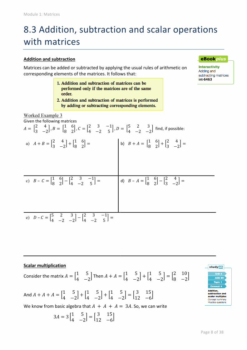
8.3 Addition, subtraction and scalar operations with matrices Addition and subtraction

Matrices can be added or subtracted by applying the usual rules of arithmetic on corresponding elements of the matrices. It follows that:

Worked Example 3 Given the following matrices

𝐴 = 2 43 −2 , 𝐵 = 1 6

8 2 , 𝐶 = 2 3 −14 −2 5 , 𝐷 = 5 2 3

4 −2 −2 find, if possible:

a) 𝐴 + 𝐵 = 2 43 −2 + 1 6

8 2 = b) 𝐵 + 𝐴 = 1 68 2 + 2 4

3 −2 =

c) 𝐵 – 𝐶 = 1 68 2 − 2 3 −1

4 −2 5 = d) 𝐵 – 𝐴 = 1 68 2 − 2 4

3 −2 =

e) 𝐷 – 𝐶 = 5 2 34 −2 −2 − 2 3 −1

4 −2 5 =

Scalar multiplication

Consider the matrix 𝐴 = 1 54 −2 Then 𝐴 + 𝐴 = 1 5

4 −2 + 1 54 −2 = 2 10

8 −2

And 𝐴 + 𝐴 + 𝐴 = 1 54 −2 + 1 5

4 −2 + 1 54 −2 = 3 15

12 −6

We know from basic algebra that 𝐴 + 𝐴 + 𝐴 = 3𝐴. So, we can write

3𝐴 = 3 1 54 −2 = 3 15

12 −6

Module 1: Matrices

of 38

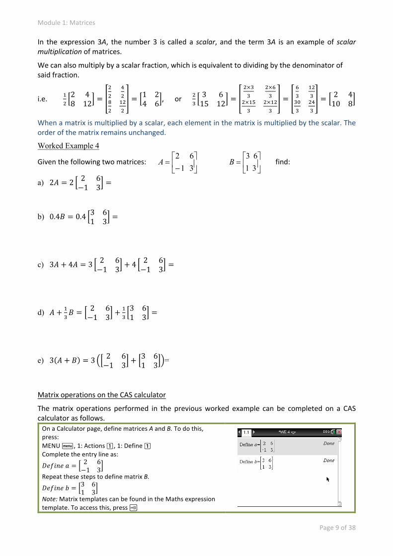
In the expression 3A, the number 3 is called a scalar, and the term 3A is an example of scalar multiplication of matrices.

We can also multiply by a scalar fraction, which is equivalent to dividing by the denominator of said fraction.

i.e. PQ2 48 12 =

QQ

RQ

SQ

PQQ

= 1 24 6 , or Q

T3 615 12 =

Q×TT

Q×UT

Q×PVT

Q×PQT

=UT

PQT

TWT

QRT

= 2 410 8

When a matrix is multiplied by a scalar, each element in the matrix is multiplied by the scalar. The order of the matrix remains unchanged.

Worked Example 4

Given the following two matrices: úû

ùêë

é-

=3162

A úû

ùêë

é=

3163

B find:

a) 2𝐴 = 2 2 6−1 3 =

b) 0.4𝐵 = 0.4 3 61 3 =

c) 3𝐴 + 4𝐴 = 3 2 6−1 3 + 4 2 6

−1 3 =

d) 𝐴 + PT𝐵 = 2 6

−1 3 + PT3 61 3 =

e) 3 𝐴 + 𝐵 = 3 2 6−1 3 + 3 6

1 3 =

Matrix operations on the CAS calculator

The matrix operations performed in the previous worked example can be completed on a CAS calculator as follows. On a Calculator page, define matrices A and B. To do this, press: MENU b, 1: Actions 1, 1: Define 1 Complete the entry line as:

𝐷𝑒𝑓𝑖𝑛𝑒 𝑎 = 2 6−1 3

Repeat these steps to define matrix B.

𝐷𝑒𝑓𝑖𝑛𝑒 𝑏 = 3 61 3

Note: Matrix templates can be found in the Maths expression template. To access this, press t

Module 1: Matrices

of 38

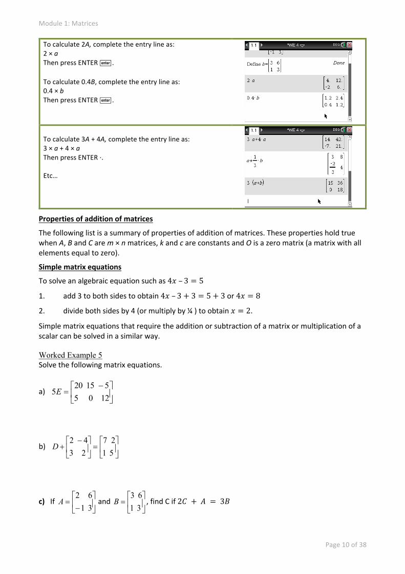
To calculate 2A, complete the entry line as: 2 × a Then press ENTER ·. To calculate 0.4B, complete the entry line as: 0.4 × b Then press ENTER ·. To calculate 3A + 4A, complete the entry line as: 3 × a + 4 × a Then press ENTER ·∙. Etc…

Properties of addition of matrices

The following list is a summary of properties of addition of matrices. These properties hold true when A, B and C are m × n matrices, k and c are constants and O is a zero matrix (a matrix with all elements equal to zero).

Simple matrix equations

To solve an algebraic equation such as 4𝑥 – 3 = 5

1. add 3 to both sides to obtain 4𝑥 – 3 + 3 = 5 + 3 or 4𝑥 = 8

2. divide both sides by 4 (or multiply by ¼ ) to obtain 𝑥 = 2.

Simple matrix equations that require the addition or subtraction of a matrix or multiplication of a scalar can be solved in a similar way. Worked Example 5 Solve the following matrix equations.

a) úû

ùêë

é -=

120551520

5E

b) úû

ùêë

é=ú

û

ùêë

é -+

5127

2342

D

c) If úû

ùêë

é-

=3162

A and úû

ùêë

é=

3163

B , find C if 2𝐶 + 𝐴 = 3𝐵

Module 1: Matrices

of 38

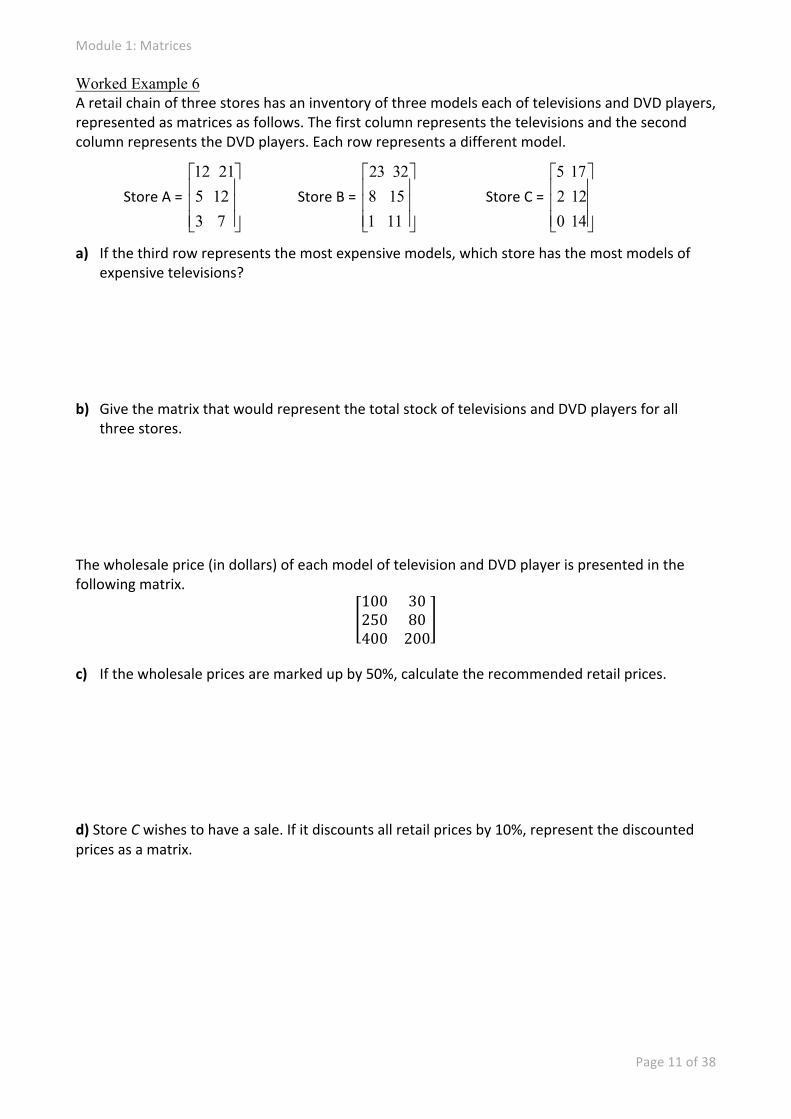
Worked Example 6 A retail chain of three stores has an inventory of three models each of televisions and DVD players, represented as matrices as follows. The first column represents the televisions and the second column represents the DVD players. Each row represents a different model.

Store A = úúú

û

ù

êêê

ë

é

731252112

Store B = úúú

û

ù

êêê

ë

é

1111583223

Store C = úúú

û

ù

êêê

ë

é

140122175

a) If the third row represents the most expensive models, which store has the most models of expensive televisions?

b) Give the matrix that would represent the total stock of televisions and DVD players for all

three stores. The wholesale price (in dollars) of each model of television and DVD player is presented in the following matrix.

100 30250 80400 200

c) If the wholesale prices are marked up by 50%, calculate the recommended retail prices. d) Store C wishes to have a sale. If it discounts all retail prices by 10%, represent the discounted prices as a matrix.

Module 1: Matrices

of 38

8.4 Multiplying matrices The multiplication rule

Two matrices can be multiplied if the number of columns in the first matrix is equal to the number of rows in the second matrix. For example

1 2 32 4 5 ×

1 22 0

3 41 6

3 −4 0 8

The number of columns in the first matrix is 3 and the number of rows in the second matrix is 3. It is possible for these two matrices to be multiplied. A way to remember this is to write the order of each matrix beside each other as shown.

2 ´ 𝟑 ´ 𝟑 ´ 4

If the two inner numbers (shown in bold) are the same, it is possible to multiply the matrices.

The order of the resulting matrix is the outer two numbers.

In the multiplication shown above, the order is ____________

If the two inner numbers are not the same, then it will not be possible to multiply the matrices.

Can the following matrices be multiplied?

1 2 32 0 53 −4 2

× 1 2 32 4 6

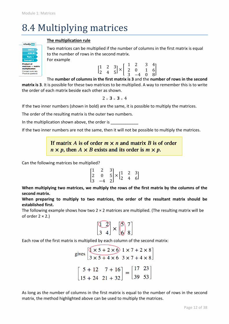
When multiplying two matrices, we multiply the rows of the first matrix by the columns of the second matrix. When preparing to multiply to two matrices, the order of the resultant matrix should be established first. The following example shows how two 2 × 2 matrices are multiplied. (The resulting matrix will be of order 2 × 2.)

Each row of the first matrix is multiplied by each column of the second matrix:

As long as the number of columns in the first matrix is equal to the number of rows in the second matrix, the method highlighted above can be used to multiply the matrices.

Module 1: Matrices

of 38

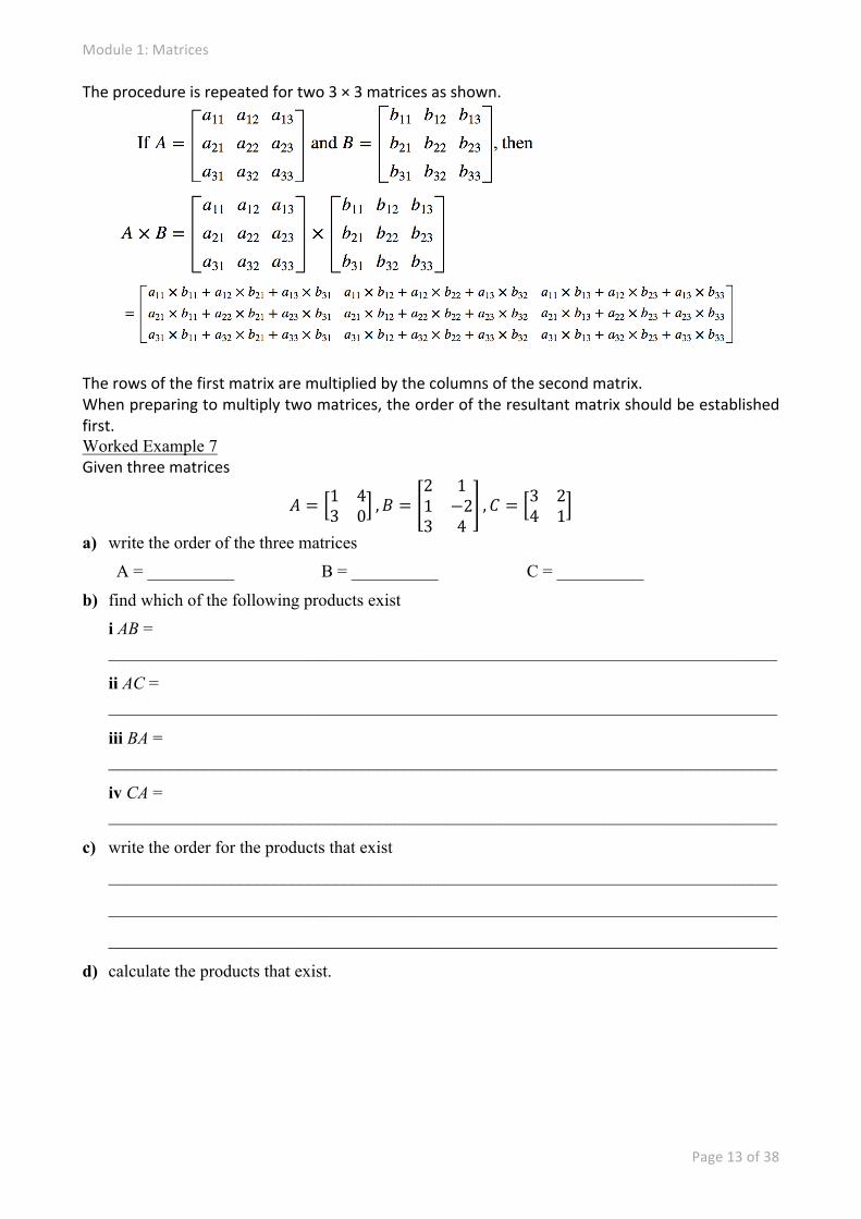
The procedure is repeated for two 3 × 3 matrices as shown.

The rows of the first matrix are multiplied by the columns of the second matrix. When preparing to multiply two matrices, the order of the resultant matrix should be established first. Worked Example 7 Given three matrices

𝐴 = 1 43 0 , 𝐵 =

2 11 −23 4

, 𝐶 = 3 24 1

a) write the order of the three matrices A = __________ B = __________ C = __________

b) find which of the following products exist i AB = _____________________________________________________________________________

ii AC = _____________________________________________________________________________

iii BA = _____________________________________________________________________________

iv CA = _____________________________________________________________________________

c) write the order for the products that exist _____________________________________________________________________________

_____________________________________________________________________________

_____________________________________________________________________________

d) calculate the products that exist.

Module 1: Matrices

of 38

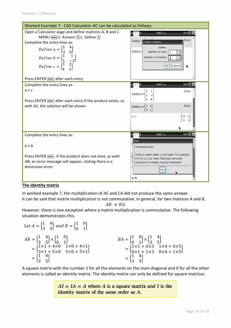
Worked Example 7 -‐ CAS Calculator AC can be calculated as follows. Open a Calculator page and define matrices A, B and C.

MENU b1: Actions 11: Define 1 Complete the entry lines as:

𝐷𝑒𝑓𝑖𝑛𝑒 𝑎 = 1 43 0

𝐷𝑒𝑓𝑖𝑛𝑒 𝑏 = 1 11 −2

𝐷𝑒𝑓𝑖𝑛𝑒 𝑐 = 3 24 1

Press ENTER · after each entry. Complete the entry lines as: a × c

Press ENTER · after each entry If the product exists, as with AC, the solution will be shown. Complete the entry lines as:

a × b

Press ENTER ·. If the product does not exist, as with AB, an error message will appear, stating there is a dimension error.

The identity matrix

In worked example 7, the multiplication of AC and CA did not produce the same answer. It can be said that matrix multiplication is not commutative. In general, for two matrices A and B,

𝐴𝐵 ≠ 𝐵𝐴. However, there is one exception where a matrix multiplication is commutative. The following situation demonstrates this.

Let 𝐴 = 1 43 5 𝑎𝑛𝑑 𝐵 = 1 0

0 1

𝐴𝐵 = 1 43 5 × 1 0

0 1

= 1×1 + 4×0 1×0 + 4×13×1 + 5×0 3×0 + 5×1

= 1 43 5

𝐵𝐴 = 1 00 1 × 1 4

3 5

= 1×1 + 0×3 1×4 + 0×50×1 + 1×3 0×4 + 1×5

= 1 43 5

A square matrix with the number 1 for all the elements on the main diagonal and 0 for all the other elements is called an identity matrix. The identity matrix can only be defined for square matrices

Module 1: Matrices

of 38

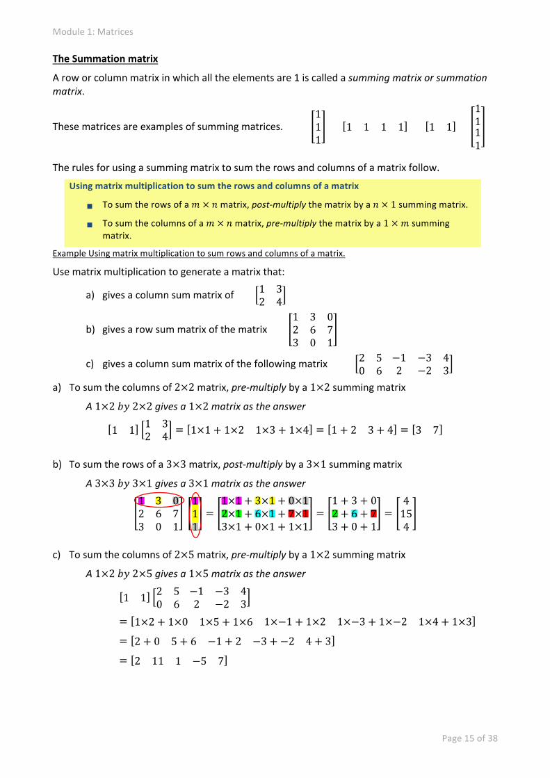
The Summation matrix

A row or column matrix in which all the elements are 1 is called a summing matrix or summation matrix.

These matrices are examples of summing matrices. 111 1 1 1 1 1 1

1111

The rules for using a summing matrix to sum the rows and columns of a matrix follow.

Using matrix multiplication to sum the rows and columns of a matrix

§ To sum the rows of a 𝑚 × 𝑛 matrix, post-‐multiply the matrix by a 𝑛 × 1 summing matrix.

§ To sum the columns of a 𝑚 × 𝑛 matrix, pre-‐multiply the matrix by a 1 × 𝑚 summing matrix.

Example Using matrix multiplication to sum rows and columns of a matrix.

Use matrix multiplication to generate a matrix that:

a) gives a column sum matrix of 1 32 4

b) gives a row sum matrix of the matrix 1 3 02 6 73 0 1

c) gives a column sum matrix of the following matrix 2 50 6

−1 −3 42 −2 3

a) To sum the columns of 2×2 matrix, pre-‐multiply by a 1×2 summing matrix

A 1×2 𝑏𝑦 2×2 gives a 1×2 matrix as the answer

1 1 1 32 4 = 1×1 + 1×2 1×3 + 1×4 = 1 + 2 3 + 4 = 3 7

b) To sum the rows of a 3×3 matrix, post-‐multiply by a 3×1 summing matrix

A 3×3 𝑏𝑦 3×1 gives a 3×1 matrix as the answer 1 3 02 6 73 0 1

111=

1×1 + 3×1 + 0×12×1 + 6×1 + 7×13×1 + 0×1 + 1×1

=1 + 3 + 02 + 6 + 73 + 0 + 1

=4154

c) To sum the columns of 2×5 matrix, pre-‐multiply by a 1×2 summing matrix

A 1×2 𝑏𝑦 2×5 gives a 1×5 matrix as the answer

1 1 2 50 6

−1 −3 42 −2 3

= 1×2 + 1×0 1×5 + 1×6 1×−1 + 1×2 1×−3 + 1×−2 1×4 + 1×3

= 2 + 0 5 + 6 −1 + 2 −3 + −2 4 + 3

= 2 11 1 −5 7

Module 1: Matrices

of 38

Permutation matrix

Recall that a binary matrix is a matrix that consists of elements that are all either 0 or 1. Just like the identity matrix being a special type of a binary matrix, a permutation matrix is another special type. A permutation matrix is an n × n matrix that is a row or column permutation of the identity matrix. Permutation matrices reorder the rows or columns of another matrix via multiplication. If Q is a matrix and P is a permutation matrix, then:

• QP is a column permutation of Q • PQ is a row permutation of Q post-‐multiplying gives a column permutation and pre-‐multiplying gives a row permutation.

Given 𝑄 =1 2 34 5 67 8 9

and 𝑃 =0 0 11 0 00 1 0

, then:

• 𝑄𝑃 =2 3 15 6 48 9 7

which is a column permutation of 𝑄. This is because the permutation matrix

𝑃 =0 0 11 0 00 1 0

has 1’s in the positions a13, a21 and a32, and so column 1 → 3, column 2 → 1 and

column 3 → 2.

• 𝑃𝑄 =7 8 91 2 34 5 6

which is a row permutation of 𝑄. This is because the permutation matrix

𝑃 =0 0 11 0 00 1 0

has 1s in the positions a13, a21 and a32, the row changes are row 3 → 1, row 1 →

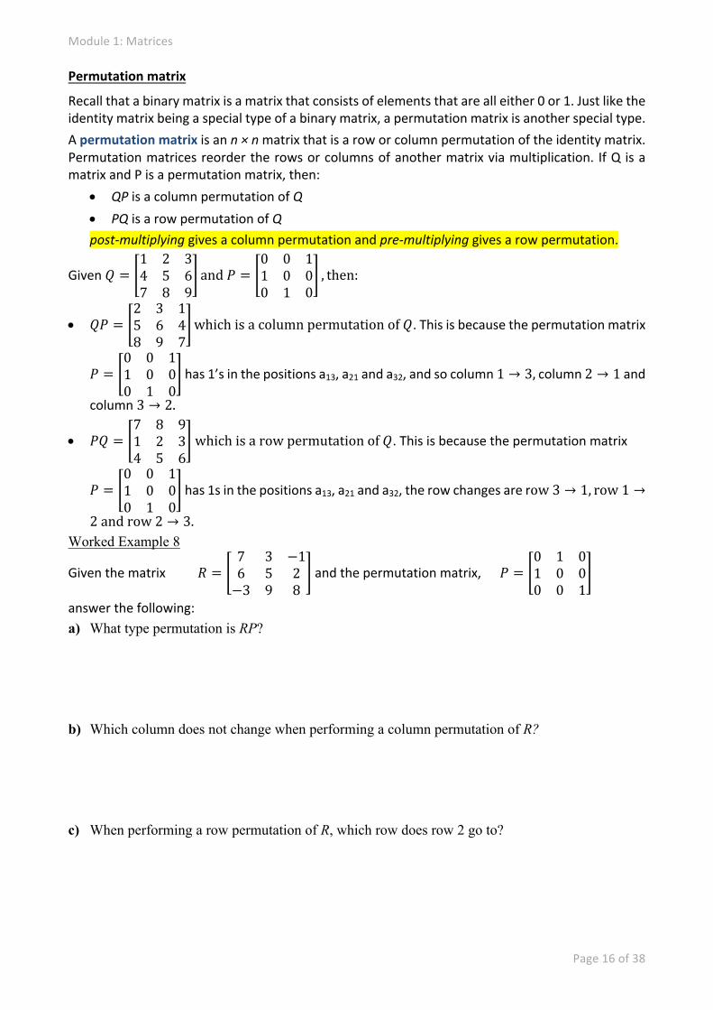
2 and row 2 → 3. Worked Example 8

Given the matrix 𝑅 =7 3 −16 5 2−3 9 8

and the permutation matrix, 𝑃 =0 1 01 0 00 0 1

answer the following: a) What type permutation is RP?

b) Which column does not change when performing a column permutation of R?

c) When performing a row permutation of R, which row does row 2 go to?

Module 1: Matrices

of 38

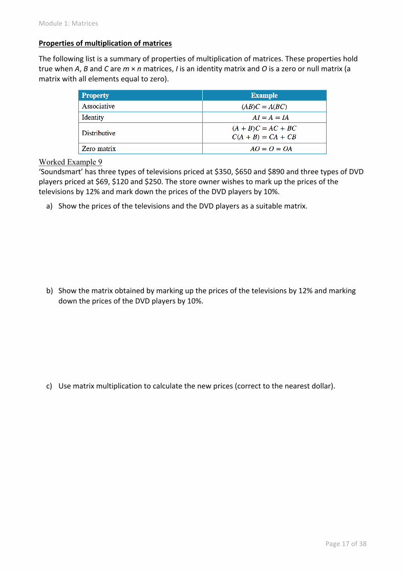
Properties of multiplication of matrices

The following list is a summary of properties of multiplication of matrices. These properties hold true when A, B and C are m × n matrices, I is an identity matrix and O is a zero or null matrix (a matrix with all elements equal to zero).

Worked Example 9 ‘Soundsmart’ has three types of televisions priced at $350, $650 and $890 and three types of DVD players priced at $69, $120 and $250. The store owner wishes to mark up the prices of the televisions by 12% and mark down the prices of the DVD players by 10%.

a) Show the prices of the televisions and the DVD players as a suitable matrix.

b) Show the matrix obtained by marking up the prices of the televisions by 12% and marking down the prices of the DVD players by 10%.

c) Use matrix multiplication to calculate the new prices (correct to the nearest dollar).

Module 1: Matrices

of 38

Worked Example 10 The number of desktop and notebook computers sold by four stores is given in the table below. If the desktop computers were priced at $1500 each and the notebook computers at $2300 each, find using matrix operations: a) the total sales figures of each computer at each store b) the total sales figures for each store c) the store that had the highest sales figures for

i desktop computers ii total sales.

Module 1: Matrices

of 38

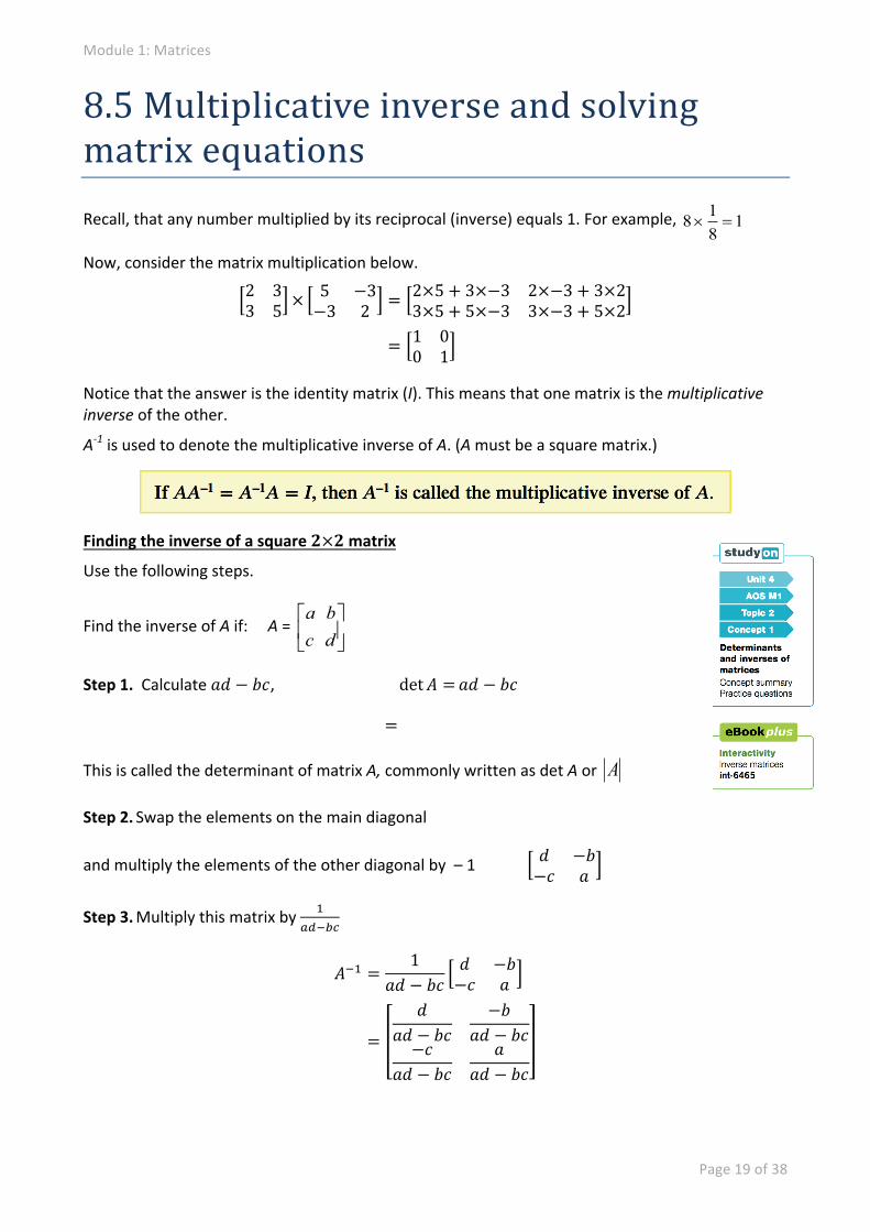
8.5 Multiplicative inverse and solving matrix equations Recall, that any number multiplied by its reciprocal (inverse) equals 1. For example, 1

818 =´

Now, consider the matrix multiplication below. 2 33 5 × 5 −3

−3 2 = 2×5 + 3×−3 2×−3 + 3×23×5 + 5×−3 3×−3 + 5×2

= 1 00 1

Notice that the answer is the identity matrix (I). This means that one matrix is the multiplicative inverse of the other.

A-‐1 is used to denote the multiplicative inverse of A. (A must be a square matrix.)

Finding the inverse of a square 𝟐×𝟐 matrix

Use the following steps.

Find the inverse of A if: A = úû

ùêë

édcba

Step 1. Calculate 𝑎𝑑 − 𝑏𝑐, det 𝐴 =𝑎𝑑 − 𝑏𝑐

=

This is called the determinant of matrix A, commonly written as det A or A

Step 2. Swap the elements on the main diagonal

and multiply the elements of the other diagonal by – 1 𝑑 −𝑏−𝑐 𝑎

Step 3. Multiply this matrix by Pmnopq

𝐴oP =1

𝑎𝑑 − 𝑏𝑐𝑑 −𝑏−𝑐 𝑎

=

𝑑𝑎𝑑 − 𝑏𝑐

−𝑏𝑎𝑑 − 𝑏𝑐

−𝑐𝑎𝑑 − 𝑏𝑐

𝑎𝑎𝑑 − 𝑏𝑐

Module 1: Matrices

of 38

Worked Example 11 Calculate the determinants of the following matrices.

𝐴 = 3 42 −3 𝐵 = 6 3

2 2 𝐶 = 4 83 6

∆=

∆=

∆=

Singular matrices

Notice that the determinant of matrix C in Worked example 11 was 0. For any matrix that has a determinant of 0, it is impossible for an inverse to exist. This is because P

W is undefined. A matrix with

a determinant equal to 0 is called a singular matrix. If the determinant of a matrix is not 0, it is called a regular matrix.

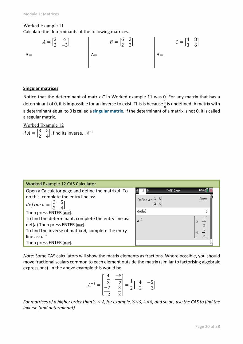
Worked Example 12 If 𝐴 = 3 5

2 4 , find its inverse, 1-A Worked Example 12 CAS Calculator Open a Calculator page and define the matrix A. To do this, complete the entry line as:

𝑑𝑒𝑓𝑖𝑛𝑒 𝑎 = 3 52 4

Then press ENTER ·. To find the determinant, complete the entry line as: det(a) Then press ENTER ·. To find the inverse of matrix A, complete the entry line as: a−1 Then press ENTER ·.

Note: Some CAS calculators will show the matrix elements as fractions. Where possible, you should move fractional scalars common to each element outside the matrix (similar to factorising algebraic expressions). In the above example this would be:

𝐴oP = 42

−5 2

−2 2

32

=12 4 −5−2 3

For matrices of a higher order than 2 × 2, for example, 3×3, 4×4, and so on, use the CAS to find the inverse (and determinant).

Module 1: Matrices

of 38

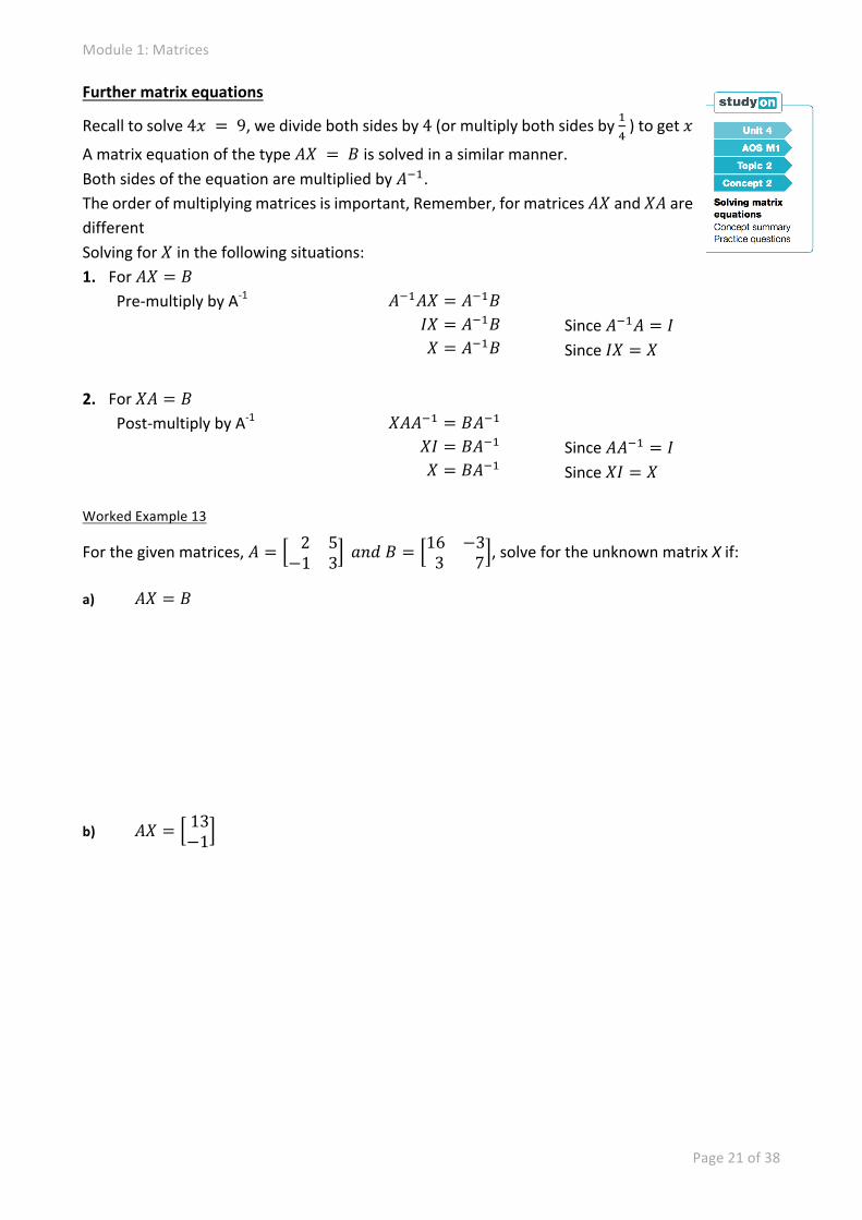
Further matrix equations

Recall to solve 4𝑥 = 9, we divide both sides by 4 (or multiply both sides by PR ) to get 𝑥

A matrix equation of the type 𝐴𝑋 = 𝐵 is solved in a similar manner. Both sides of the equation are multiplied by 𝐴oP. The order of multiplying matrices is important, Remember, for matrices 𝐴𝑋 and 𝑋𝐴 are different Solving for 𝑋 in the following situations: 1. For 𝐴𝑋 = 𝐵

Pre-‐multiply by A-‐1 𝐴oP𝐴𝑋 = 𝐴oP𝐵 𝐼𝑋 = 𝐴oP𝐵 𝑋 = 𝐴oP𝐵

Since 𝐴oP𝐴 = 𝐼 Since 𝐼𝑋 = 𝑋

2. For 𝑋𝐴 = 𝐵

Post-‐multiply by A-‐1 𝑋𝐴𝐴oP = 𝐵𝐴oP 𝑋𝐼 = 𝐵𝐴oP 𝑋 = 𝐵𝐴oP

Since 𝐴𝐴oP = 𝐼 Since 𝑋𝐼 = 𝑋

Worked Example 13

For the given matrices, 𝐴 = 2 5−1 3 𝑎𝑛𝑑 𝐵 = 16 −3

3 7 , solve for the unknown matrix X if: a) 𝐴𝑋 = 𝐵

b) 𝐴𝑋 = 13−1

Module 1: Matrices

of 38

8.6 Dominance and communication matrices A directed graph (or digraph) is a graph or network where every edge has a direction. Directed graphs can be used to represent many situations, such as traffic flow, competitions between teams or the order of activities in a production line.

Reachability

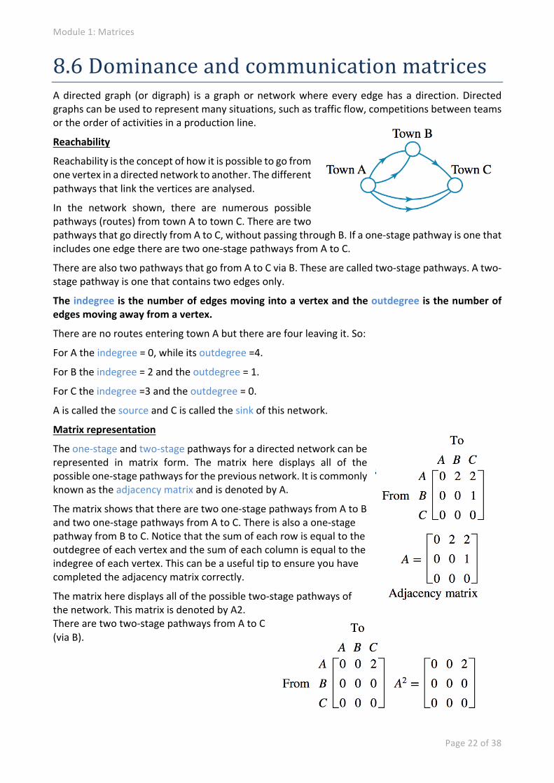
Reachability is the concept of how it is possible to go from one vertex in a directed network to another. The different pathways that link the vertices are analysed.

In the network shown, there are numerous possible pathways (routes) from town A to town C. There are two pathways that go directly from A to C, without passing through B. If a one-‐stage pathway is one that includes one edge there are two one-‐stage pathways from A to C.

There are also two pathways that go from A to C via B. These are called two-‐stage pathways. A two-‐stage pathway is one that contains two edges only.

The indegree is the number of edges moving into a vertex and the outdegree is the number of edges moving away from a vertex.

There are no routes entering town A but there are four leaving it. So:

For A the indegree = 0, while its outdegree =4.

For B the indegree = 2 and the outdegree = 1.

For C the indegree =3 and the outdegree = 0.

A is called the source and C is called the sink of this network.

Matrix representation

The one-‐stage and two-‐stage pathways for a directed network can be represented in matrix form. The matrix here displays all of the possible one-‐stage pathways for the previous network. It is commonly known as the adjacency matrix and is denoted by A.

The matrix shows that there are two one-‐stage pathways from A to B and two one-‐stage pathways from A to C. There is also a one-‐stage pathway from B to C. Notice that the sum of each row is equal to the outdegree of each vertex and the sum of each column is equal to the indegree of each vertex. This can be a useful tip to ensure you have completed the adjacency matrix correctly.

The matrix here displays all of the possible two-‐stage pathways of the network. This matrix is denoted by A2. There are two two-‐stage pathways from A to C (via B).

Module 1: Matrices

of 38

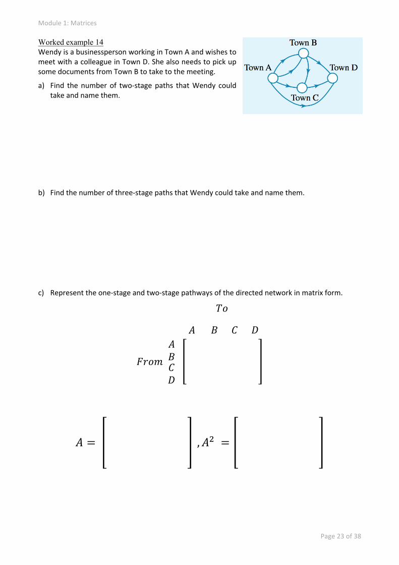
Worked example 14 Wendy is a businessperson working in Town A and wishes to meet with a colleague in Town D. She also needs to pick up some documents from Town B to take to the meeting.

a) Find the number of two-‐stage paths that Wendy could take and name them.

b) Find the number of three-‐stage paths that Wendy could take and name them.

c) Represent the one-‐stage and two-‐stage pathways of the directed network in matrix form.

𝑇𝑜

𝐴 𝐵 𝐶 𝐷

𝐹𝑟𝑜𝑚 𝐴𝐵𝐶𝐷

𝐴 = , 𝐴Q =

Module 1: Matrices

of 38

Dominance

If an edge in a directed network moves from A to B, then it can be said that A is dominant, or has a greater influence, over B. If an edge moves from B to C, then B is dominant over C. However, we often wish to find the dominant vertex in a network; that is, the vertex that holds the most influence over all the other vertices.

This may be clearly seen by inspection, by examining the pathways between the vertices. It may be the vertex that has the most edges moving away from it. Generally speaking, if there are more ways to go from A to B than there are to go from B to A, then A is the dominant vertex.

In Worked example 14, town A is dominant over all the other vertices (towns) as it has edges moving to each of the other vertices. Similarly, B has edges moving to C and D, so B is dominant over C and D and C is dominant over D. Using this inspection technique, we can list the vertices in order of dominance from A then B then C and finally D.

A more formal approach to determine a dominant vertex can be taken using matrix representation. Using the matrices from Worked example 14, this approach is outlined below.

Take the matrices that represent the one-‐stage pathways (the adjacency matrix, A) and two-‐stage pathways (A2) and add them together. (When adding matrices, simply add the numbers in the corresponding positions.)

The resulting matrix, which we will call the dominance matrix, consists of all the possible one-‐ and two-‐stage pathways in the network. By taking the sum of each row in this matrix, we can determine the dominant vertex. The dominant vertex belongs to the row that has the highest sum.

The first row corresponds with vertex A and has a sum of 9. Row 2 (vertex B) has a sum of 3, row 3 (vertex C) has a sum of 1 and row 4 (vertex D) has a sum of 0. The highest sum is 9, so the dominant vertex is A. The order of dominance is the same as for the inspection technique described earlier.

This formal approach just described is not the only technique used to determine dominance in a network. Other approaches are possible, but this section will concentrate only on the inspection technique and summing the rows of the matrix that results from A + A2.

The concept of dominance can be applied to various situations such as transportation problems, competition problems and situations involving relative positions.

Module 1: Matrices

of 38

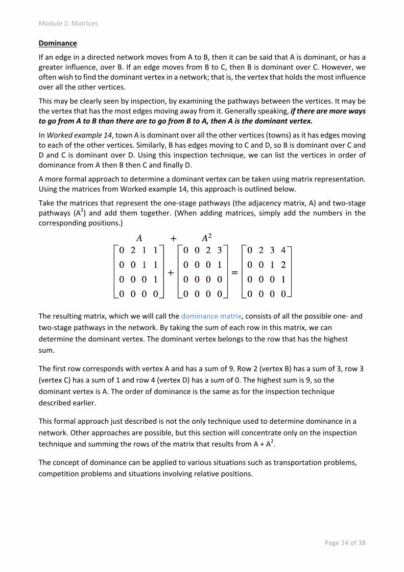
Worked Example 15 The results of a round robin (each competitor plays each other once) tennis competition are represented by the directed graph at right.

a) By inspection, determine the dominant vertex (dominant competitor); that is, the winner. Rank the competitors in finishing order.

b) Confirm your answer to part a by finding the matrix, A + A2, and summing the rows of this matrix.

𝐴 =

𝐴Q =

+ =

Communication

From Worked example 15 we looked at results of a round robin tennis competition. This is where one competitor either wins or loses to another competitor. Thus, the network has arrows going only one way. A communication network has the ability of the arrows to travel both ways. A communication network contains a set of people where they can have a one-‐way or two-‐way communication link. A two-‐way communication link could be via phone. We can set up communication matrices from communication networks.

Module 1: Matrices

of 38

Worked Example 16 Find the communication matrix from the following communication network.

𝐴 𝐵 𝐶 𝐷

𝐴𝐵𝐶𝐷

𝐴 𝐵 𝐶 𝐷

𝐴𝐵𝐶𝐷

𝐴 𝐵 𝐶 𝐷

𝐴𝐵𝐶𝐷

𝐴 𝐵 𝐶 𝐷

𝐴𝐵𝐶𝐷

𝐴 𝐵 𝐶 𝐷

𝐴𝐵𝐶𝐷

𝐴 𝐵 𝐶 𝐷

𝐴𝐵𝐶𝐷

Module 1: Matrices

of 38

8.7 Application of matrices to simultaneous equations Matrices can be used to solve linear simultaneous equations. The following technique demonstrates how to use matrices to solve simultaneous equations involving two unknowns.

Consider a pair of simultaneous equations in the form:

𝑎𝑥 + 𝑏𝑦 = 𝑒 𝑐𝑥 + 𝑑𝑦 = 𝑓

The equations can be expressed as a matrix equation in the form 𝐴𝑋 = 𝐵

𝑎 𝑏𝑐 𝑑

𝑥𝑦 =

𝑒𝑓

𝐴 = 𝑎 𝑏𝑐 𝑑 is called the coefficient matrix, 𝑋 =

𝑥𝑦 and 𝐵 =

𝑒𝑓

Notes 1. A is the matrix of the coefficients of x and y in the simultaneous equations. 2. X is the matrix of the pronumerals used in the simultaneous equations. 3. B is the matrix of the numbers on the right-‐hand side of the simultaneous equations.

As we have seen from Exercise 8.5, an equation in the form AX = B can be solved by pre-‐multiplying both sides by A–1.

𝐴oP𝐴𝑋 = 𝐴oP𝐵 𝑋 = 𝐴oP𝐵

Worked Example 17(a) Solve the two simultaneous linear equations by matrix methods

2𝑥 + 3𝑦 = 13 5𝑥 + 2𝑦 = 16

Module 1: Matrices

of 38

Simultaneous equations involving more than two unknowns can be converted to matrix equations in a similar manner to the methods described previously. However, the CAS calculator will be used to find the value of the pronumerals.

When solving simultaneous equations, one equation for each unknown is needed.

The following is an ancient Chinese Maths problem:

There are three types of corn, of which three bundles of the first, two of the second, and one of the third make 39 measures. Two of the first, three of the second and one of the third make 34 measures. And one of the first, two of the second and three of the third make 26 measures. How many measures of corn are contained in one bundle of each type?

This information can be converted to equations, using the pronumerals x, y and z to represent the three types of corn, as follows:

3𝑥 + 2𝑦 + 1𝑧 = 39 2𝑥 + 3𝑦 + 1𝑧 = 34 1𝑥 + 2𝑦 + 3𝑧 = 26

This can be expressed as a matrix equation 3 2 12 3 11 2 3

𝑥𝑦𝑧=

393426

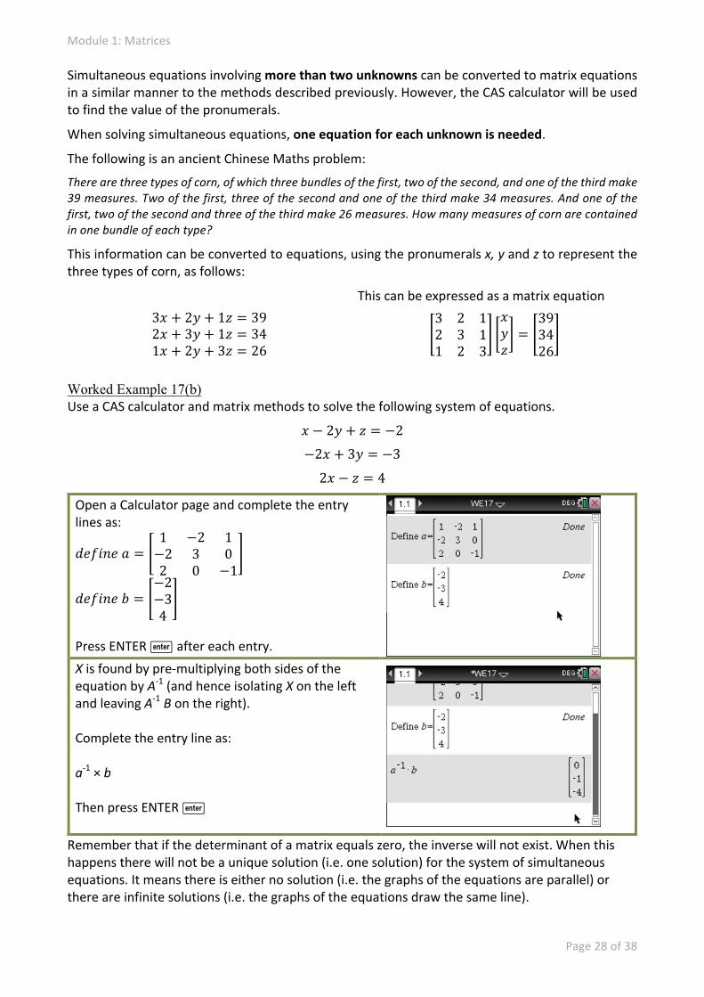
Worked Example 17(b) Use a CAS calculator and matrix methods to solve the following system of equations.

𝑥 − 2𝑦 + 𝑧 = −2 −2𝑥 + 3𝑦 = −3 2𝑥 − 𝑧 = 4

Open a Calculator page and complete the entry lines as:

𝑑𝑒𝑓𝑖𝑛𝑒 𝑎 =1 −2 1−2 3 02 0 −1

𝑑𝑒𝑓𝑖𝑛𝑒 𝑏 =−2−34

Press ENTER · after each entry. X is found by pre-‐multiplying both sides of the equation by A-‐1 (and hence isolating X on the left and leaving A-‐1 B on the right). Complete the entry line as: a-‐1 × b Then press ENTER ·

Remember that if the determinant of a matrix equals zero, the inverse will not exist. When this happens there will not be a unique solution (i.e. one solution) for the system of simultaneous equations. It means there is either no solution (i.e. the graphs of the equations are parallel) or there are infinite solutions (i.e. the graphs of the equations draw the same line).

Module 1: Matrices

of 38

Dependent systems of equations

If the graphs of two or more equations coincide, that is if they are the same line, then there is no unique solution to the equations and we say that the equations are dependent. If we try to solve dependent equations using matrix methods then we would find that there would be no solution as the determinant of the coefficient matrix is 0.

Inconsistent systems of equations

If the graphs of two or more equations do not meet, that is if the lines are parallel, then there is no solution to the equations and we say that the equations are inconsistent. If we try to solve inconsistent equations using matrix methods then we would find that there would be no solution as the determinant of the coefficient matrix is 0.

Worked Example 18 Use a matrix method to decide if the simultaneous equations have a unique solution.

i 2𝑥 − 𝑦 = 8 ii 2𝑥 + 4𝑦 = 12

𝑥 + 𝑦 = 1 3𝑥 + 6𝑦 = 8

Matrix mathematics is a very efficient tool for solving problems with two or more unknowns. As a result, it is used in many areas such as engineering, computer graphics and economics. When answering problems of this type, take care to follow these steps: (a) read the problem several times to ensure you fully understand it (b) identify the unknowns and assign suitable pronumerals. (Remember that the number of

equations needed is the same as the number of unknowns.) (c) identify statements that define the equations and write the equations using the chosen

pronumerals. Align the pronumerals (d) use the matrix methods to solve the equations.

Module 1: Matrices

of 38

Worked Example 19 A bakery produces two types of bread, wholemeal and rye. The respective processing times for each batch on the dough-‐making machine are 12 minutes and 15 minutes, while the oven baking times are 16 minutes and12 minutes respectively. How many batches of each type of bread should be processed in an 8-‐hour shift so that both the dough-‐making machine and the oven are fully occupied?

Module 1: Matrices

of 38

8.8 Transition Matrices Andrei Markov was a mathematician whose name is given to a technique that calculates probability associated with the state of various transitions (which can be represented in matrix form). It answers questions such as, ‘What is the probability that it will rain today given that it rained yesterday?’ or ‘What can be said about the long-‐term prospect of rainy days?’

Powers of matrices

Throughout this section, it will be necessary to evaluatea matrix raised to the power of a particular number, forexample M3. Only square matrices can be raised to a power, as the order of a non-‐square matrix does not allowfor repeated matrix multiplication. (For example, a 2 × 3 matrix cannot be squared, because using the multiplication rule, we see the inner two numbers are not the same (2 × 3 × 2 × 3).)

Worked Example 20

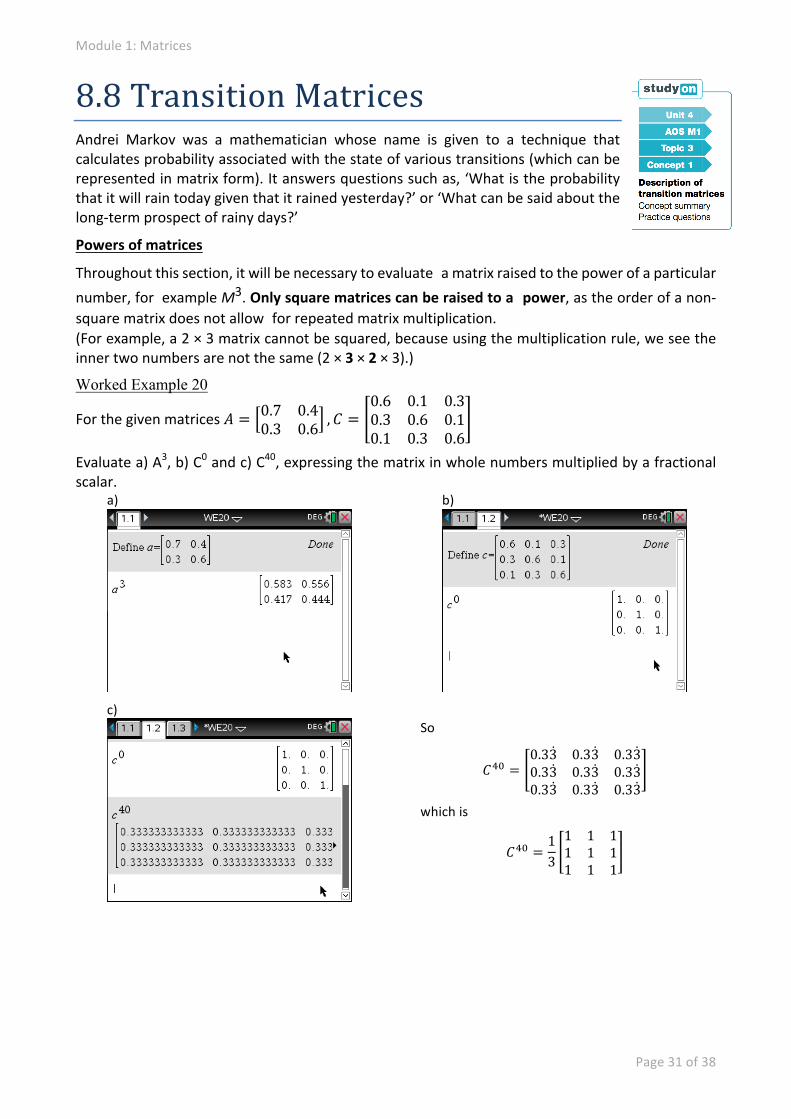
For the given matrices 𝐴 = 0.7 0.40.3 0.6 , 𝐶 =

0.6 0.1 0.30.3 0.6 0.10.1 0.3 0.6

Evaluate a) A3, b) C0 and c) C40, expressing the matrix in whole numbers multiplied by a fractional scalar.

a) b)

c)

So

𝐶RW =0.33 0.33 0.330.33 0.33 0.330.33 0.33 0.33

which is

𝐶RW =13

1 1 11 1 11 1 1

Module 1: Matrices

of 38

Markov systems and transition matrices

A Markov system (or Markov chain) is a system that investigates estimating the distribution of states of an event, given information about the current states. It also investigates the manner in which these states change from one state (condition or location) to the next, according to fixed probabilities. Matrices can be used to model such situations where:

• there are defined sets of conditions or states • there is a transition from one state to the next, where the next state’s probability is conditional on the result of the preceding outcome • the conditional probabilities for each outcome are the same on each occasion; that is, the same matrix is used for each transition • information about an initial state is given. Markov systems can be illustrated by means of a state transition statement, a table or a diagram.

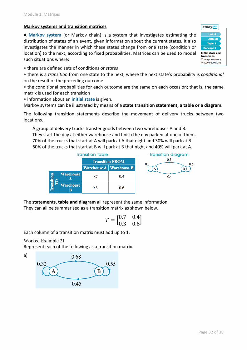
The following transition statements describe the movement of delivery trucks between two locations.

A group of delivery trucks transfer goods between two warehouses A and B. They start the day at either warehouse and finish the day parked at one of them. 70% of the trucks that start at A will park at A that night and 30% will park at B. 60% of the trucks that start at B will park at B that night and 40% will park at A.

The statements, table and diagram all represent the same information. They can all be summarised as a transition matrix as shown below.

𝑇 = 0.7 0.40.3 0.6

Each column of a transition matrix must add up to 1.

Worked Example 21 Represent each of the following as a transition matrix.

a)

Module 1: Matrices

of 38

b) There are a number of train carriages operating between two depots, North depot and South depot. At the end of each week,

40% of the carriages that started at North depot end up at South depot and 25% of the carriages that started at South depot end up at North depot.

Distribution vector and powers of the transition matrix

A distribution vector is a column vector with an entry for each state of the system. It is often referred to as the initial state matrix and is denoted by S0.

If S0 is an n × 1 initial distribution vector state matrix involving n components and T is the transition matrix, then the distribution vector after 1 transition is the matrix product T × S0.

Distribution after 1 transition: 𝑆1

= 𝑇 × 𝑆0

The distribution one stage later is given by

Distribution after 2 transitions:

𝑆2

= 𝑇 × 𝑆1 = 𝑇 × (𝑇 × 𝑆0) = (𝑇 × 𝑇) × 𝑆0

= 𝑇Q

× 𝑆0

We can continue this pattern to create a matrix recurrence relation.

The distribution after n transitions can be obtained by premultiplying 𝑆0 by 𝑇, n times or by multiplying 𝑇𝑛 by 𝑆0.

The sequence of states, 𝑆0, 𝑆1, 𝑆2, . . . , 𝑆𝑛 is called a Markov chain. Applications to marketing

Marketing organisations can predict their share of the market at any given moment. Marketing records show that when consumers are able to purchase items (groceries) stores A or B, we can associate conditional probabilities with the likelihood that they will purchase from a given store, or its competitor, depending on the store from which they had made their previous purchases over a set period, such as a month. The following worked example highlights the application of transition matrices to marketing.

Module 1: Matrices

of 38

Worked Example 22 A survey shows that 75% of the time, customers will continue to purchase their groceries from store A if they purchased their groceries from store A in the previous month, while 25% of the time consumers will change to purchasing their groceries from store B if they purchased their groceries from store A in the previous month. Similarly, the records show that 80% of the time, consumers will continue to purchase their groceries from store B if they purchased their groceries from store B in the previous month.

a) How many customers are still purchasing their groceries from A and B at the end of two months, if 300 customers started at A and 300 started at B?

b) What percentage (in whole numbers) of customers are purchasing their groceries at A and B at the end of 6 months, if 50% of the customers started at A?

Module 1: Matrices

of 38

New state matrix with culling and restocking

The new state matrix 𝑆𝑛

= 𝑇𝑛𝑆0 can be extended to include culling and restocking. This can be done by adding (restocking) or subtracting (culling) a matrix to our original new state matrix.

Worked Example 23 Betta Health Centres run concurrent Lift and Cycle fitness classes at all 3 of their gyms in FitTown. A study shows that 80% of the clients who attended a Lift class one week will attend the Lift class the next week, while the other 20% will move to the Cycle class the next week. Similarly, 70% of the clients who attended a Cycle class one week will attend the Cycle class the next week, while the other 30% will move to the Lift class the next week. The numbers are also affected by people joining and leaving the gym, with2 additional people joining the Lift classes each week and 3 additional people joining the Cycle classes each week. In the first week 55 people attended the Lift classes and 62 people attended the Cycle classes. Set up the matrix recurrence relation that would be used to find how many people attended the Lift and Cycle classes in week 2.

Module 1: Matrices

of 38

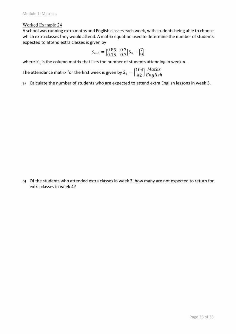
Worked Example 24 A school was running extra maths and English classes each week, with students being able to choose which extra classes they would attend. A matrix equation used to determine the number of students expected to attend extra classes is given by

𝑆|}P = 0.85 0.30.15 0.7 𝑆𝑛 − 7

9

where 𝑆𝑛 is the column matrix that lists the number of students attending in week 𝑛.

The attendance matrix for the first week is given by 𝑆P =10492

𝑀𝑎𝑡ℎ𝑠𝐸𝑛𝑔𝑙𝑖𝑠ℎ

a) Calculate the number of students who are expected to attend extra English lessons in week 3.

b) Of the students who attended extra classes in week 3, how many are not expected to return for extra classes in week 4?

Module 1: Matrices

of 38

Steady state

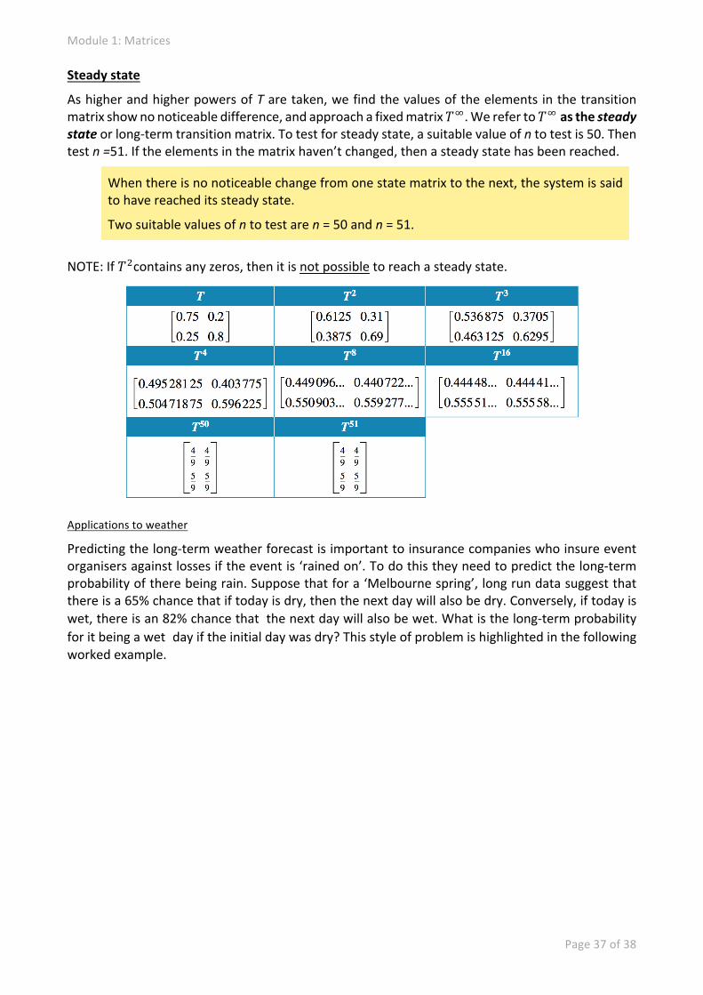
As higher and higher powers of T are taken, we find the values of the elements in the transition matrix show no noticeable difference, and approach a fixed matrix 𝑇�. We refer to 𝑇� as the steady state or long-‐term transition matrix. To test for steady state, a suitable value of n to test is 50. Then test n =51. If the elements in the matrix haven’t changed, then a steady state has been reached.

When there is no noticeable change from one state matrix to the next, the system is said to have reached its steady state.

Two suitable values of n to test are n = 50 and n = 51.

NOTE: If 𝑇Qcontains any zeros, then it is not possible to reach a steady state.

Applications to weather

Predicting the long-‐term weather forecast is important to insurance companies who insure event organisers against losses if the event is ‘rained on’. To do this they need to predict the long-‐term probability of there being rain. Suppose that for a ‘Melbourne spring’, long run data suggest that there is a 65% chance that if today is dry, then the next day will also be dry. Conversely, if today is wet, there is an 82% chance thatthe next day will also be wet. What is the long-‐term probability for it being a wetday if the initial day was dry? This style of problem is highlighted in the following worked example.

Module 1: Matrices

of 38

Worked Example 25 An insurance company needs to measure its risk if it is to underwrite a policy for a major event planned. The company used the following information about the region. The weather for the next day for a region of Victoria, from long run data, suggests that there is a 75% chance that if today is dry, then so will the next day. Conversely, if today is wet, there is a 72% chance that the next day will also be wet. This information is given in the table below.

Today is dry Today is wet

Next day dry 0.75 0.28

Next day wet 0.25 0.72

a) Find the probability it will rain in three days time if initially the day is dry. b) Find the long-‐term probability of rain if initially the day is wet. c) If the company only insures if they have the odds in their favour, will they insure this event?

Other well-‐known examples of the application of transition matrices are to population studies, stock inventory and sport.

chapter 8 matrices 2017 version 1 - paul weiser -...

Documents