chapter 8: the clamped zernike radial polynomials

213

Chapter 8: The Clamped Zernike Radial Polynomials

8.1 Introduction

When conversing between the optical and mechanical worlds, it would be desirable to be

able to compensate for image aberrations using the structural mode shapes of the

membrane optic. Such compensation might be desirable as structural mode shapes are

preferred energy states of the system, and translating the optical aberration into a

mechanical mode shape may provide another means for controlling optical image

compensation. To the optical engineer, wavefronts are measured using Zernike

polynomials. To mechanical engineers, wavefronts are more aptly described using

structural mode shapes.

The overall goal of this chapter is to demonstrate a novel set of polynomials for

describing image aberrations. Each of these polynomials is zero at the membrane edge,

consequently bridging the gap between the mechanical and optical worlds of the

membrane lens. In the first portion of this chapter, we will review the orthonormal mode

shapes of a clamped circular membrane. Then, we will introduce the Zernike

polynomials, a complete set of polynomials that are traditionally used in the optical world

to describe image aberrations. Having established both, we will next discuss the use of a

uniform actuation pressure and boundary displacement to statically correct the image

aberration. We will then develop a novel set of polynomials, the clamped Zernike radial

polynomials, and show their advantage over the traditional Zernike polynomials. Finally,

we will describe the Fourier expansion of the clamped Zernike polynomials using the

basis formed by the orthonormal mode shapes of the circular membrane and demonstrate

analytically how these shapes could be used to make a nearly 100% effective deformable

membrane lens for adaptive optics. This chapter reflects collaborative work between the

Air Force Research Lab Directed Energy Directorate (AFRL/DE) and Virginia Tech in

the area of adaptive membrane optics.

214

8.2 Orthonormal Mode Shapes of a Clamped Circular Membrane

The mode shapes of a clamped circular membrane are given by the solution to Bessel’s

equation,

012

22

2

2

=

−++ R

rdrdR

rdrRd µβ , (8.1)

where Equation 8.1 is the spatial portion of the partial differential equation governing the

membrane’s transverse dynamics. The solutions to Equation 8.1 are given by

...2,1,)sin()(),(...2,1,)cos()(),(

...2,1)(),( 0000

==Ψ==Ψ

==Ψ

nmmrJArnmmrJAr

nrJAr

mnmmnsmns

mnmmncmnc

nnn

θβθθβθ

βθ (8.2)

Equations 8.2 emphasize that the clamped circular membrane has symmetric mode

shapes, ),(0 θrnΨ , that are unique, whereas the asymmetric mode shapes, ),( θrmncΨ and

),( θrmnsΨ , are degenerate.

Next, we wish to normalize the mode shapes given by Equations 8.2. First, we will

normalize the symmetric mode shapes. Following the procedure as outlined by

Meirovich (1997), we write:

( ) 12

0 00

200

20 ==ΩΨ ∫ ∫∫

Ω

π

θβρρa

nnn rdrdrJAd . (8.3)

Evaluating the integral and solving for the constant nA0 we get:

( ) 1)( 02

120

22

0 00

20

20 ==∫ ∫ aJAardrdrJA nn

a

nn βρπθβρπ

, (8.4)

215

and

πρβ )(1

010 aaJ

An

n = . (8.5)

Following the same procedure for the asymmetric modes, we get:

( ) 1)(2

)(cos 21

222

0 0

222 == +∫ ∫ aJAardrdmrJA mnmmnc

a

mnmmnc βρπθθβρπ

, (8.6)

thus giving us:

πρβ )(2

1 aaJAA

mnmmnsmnc

+

== . (8.7)

Having found the constants given by Equations 8.5 and 8.7, we now have a set of

orthogonal and normalized (hence, orthonormal) mode shapes. By orthonormal, it means

that the mode shapes demonstrate the following property:

≠=

=ΩΨΨ∫Ω ji

jidji 0

1. (8.8)

This property will help simplify our analysis in subsequent sections.

216

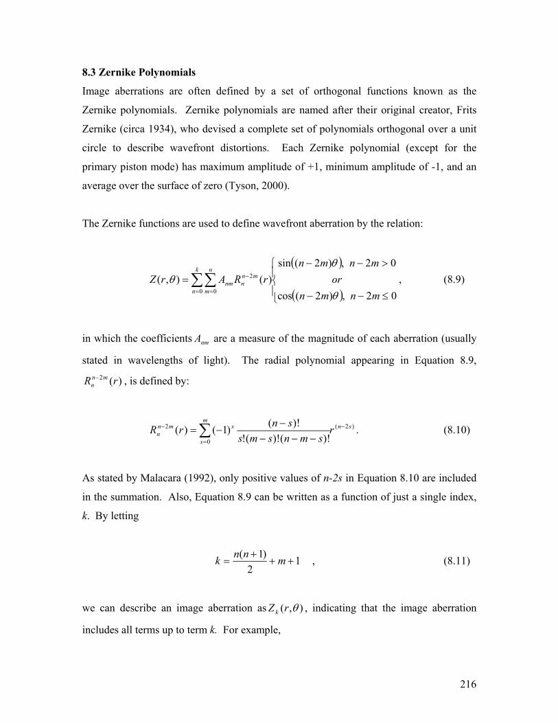
8.3 Zernike Polynomials

Image aberrations are often defined by a set of orthogonal functions known as the

Zernike polynomials. Zernike polynomials are named after their original creator, Frits

Zernike (circa 1934), who devised a complete set of polynomials orthogonal over a unit

circle to describe wavefront distortions. Each Zernike polynomial (except for the

primary piston mode) has maximum amplitude of +1, minimum amplitude of -1, and an

average over the surface of zero (Tyson, 2000).

The Zernike functions are used to define wavefront aberration by the relation:

( )

( )∑∑= =

−

≤−−

>−−=

k

n

n

m

mnnnm

mnmnor

mnmnrRArZ

0 0

2

02,)2(cos

02,)2(sin)(),(

θ

θθ , (8.9)

in which the coefficients nmA are a measure of the magnitude of each aberration (usually

stated in wavelengths of light). The radial polynomial appearing in Equation 8.9,

)(2 rR mnn− , is defined by:

)2(

0

2

)!()!(!)!()1()( sn

m

s

smnn r

smnsmssnrR −

=

− ∑ −−−−

−= . (8.10)

As stated by Malacara (1992), only positive values of n-2s in Equation 8.10 are included

in the summation. Also, Equation 8.9 can be written as a function of just a single index,

k. By letting

12

)1(++

+= mnnk , (8.11)

we can describe an image aberration as ),( θrZ k , indicating that the image aberration

includes all terms up to term k. For example,

217

θθθθ 2sincossin1),( 24 rrrrZ +++= . (8.12)

Table 8.1 describes the first nine Zernike polynomials. A plot of these Zernike shape

functions can be found in Figure 8.1.

Table 8.1. Description of the first nine Zernike polynomials.

n m k Zernike Polynomial Description

0 0 1 1 Piston

1 0 2 θsinr Tilt about x axis

1 1 3 θcosr Tilt about y axis

2 0 4 θ2sin2r Astigmatism

2 1 5 12 2 −r Defocus

2 2 6 θ2cos2r Astigmatism

3 0 7 θ3sin3r Trefoil

3 1 8 ( ) θsin23 3 rr − Coma

3 2 9 ( ) θcos23 3 rr − Coma

218

Figure 8.1. Sample plots of the Zernike polynomials describing particular wave

front aberrations.

It is also important to point out that when the quantity n-2m is zero, the theta dependent

portion of the Zernike polynomial drops out, leaving only a polynomial that is a function

of the radius, r. The piston and defocus terms are examples of this rule (refer to Table

8.1). Further, when m = 0, the radial Zernike polynomials simplify to monomials of

degree n, such that

nn

n rrR =)( . (8.13)

We have now established the optical space and the modal space for a membrane lens.

Next, we will look at using uniform pressure and boundary displacement to deform the

surface of the membrane to correct for any image aberration. This original concept has

been proposed by the AFRL/DE.

219

8.4 Static Image Aberration Compensation

To properly correct for image aberrations using a deformable mirror, geometrical optics

suggests that the required displacement is half of the wavefront aberration (Malacara,

1992), namely:

),ˆ(21),ˆ( θθ rZrw = . (8.14)

Here, we introduce the non-dimensional variablearr =ˆ , where a is the radius of the

membrane lens.

As previously derived, the equation of motion governing the transverse dynamics of a

circular membrane is given by

2

2

22 1

tw

cwr

∂∂

=∇ θ . (8.15)

If a uniform pressure is acting on the interior surface of the membrane, then the

difference between the top and bottom surface pressures, which we will denote

as ),,( trp θ∆ , enters into the equation of motion as a forcing function. Similarly, we can

also assume for our analysis that a distributed, non-uniform pressure, ),,( trpe θ , is able to

act on the membrane. This non-uniform pressure may appear as an electrostatic pressure,

and would be used to eliminate any remaining residual aberrations. The electrostatic

pressure term, ),,( trpe θ , enters the equation of motion in the same manner as the

uniform pressure term. Assuming that the incoming wavefront aberrations are changing

slowly enough for the membrane to achieve a new, static equilibrium position, then

Equation 8.15 becomes

02 =+∆

+∇T

ppw erθ , (8.16)

220

where T is the applied tensile loading to the membrane. We can non-dimensionalize

Equation 8.16 by introducing the variable r such that Equation 8.16 becomes

2ˆ

2 aT

ppw er

+∆−=∇ θ , (8.17)

where the Laplacian in dimensionless coordinates is given by

2

2

22

2

22

2

ˆ2

ˆ1

ˆˆ

ˆˆ1

ˆ1

ˆˆ1

ˆ θθθ

∂∂

+

∂∂

∂∂

=∂∂

+∂∂

+∂∂

=∇w

rrwr

rrw

rrw

rrwwr . (8.18)

For the remainder of this chapter, we will assume that the measured image aberration

consists of Zernike polynomials up to the 5th degree, so that we have

.5sin)ˆ(3sin)ˆ(

sin)ˆ(cos)ˆ(3cos)ˆ(5cos)ˆ(

4sin)ˆ(2sin)ˆ()ˆ(2cos)ˆ(

4cos)ˆ(3sin)ˆ(sin)ˆ(cos)ˆ(3cos)ˆ(

2sin)ˆ()ˆ()2cos()ˆ(sin)ˆ(cos)ˆ(),ˆ(

5555

3554

1553

1552

3551

5550

4444

2443

0442

2441

4440

3333

1332

1331

3330

2222

0221

2220

1111

111000

θθ

θθθθ

θθθ

θθθθθ

θθθθθ

rRArRA

rRArRArRArRA

rRArRArRArRA

rRArRArRArRArRA

rRArRArRArRArRAArZ

−−

−+++

−−++

+−−++

−++−+=

(8.19)

To help simplify our analysis, we substitute in the monomials (Equation 8.13) and the

other radial polynomials (for example, see Table 13.1 in Malacara (1992)), as given by

3535

3515

2424

313

2404

202

ˆ4ˆ5,ˆ3ˆ12ˆ10

,ˆ3ˆ4,ˆ2ˆ3

,1ˆ6ˆ6,1ˆ2

rrRrrrR

rrRrrR

rrRrR

−=+−=

−=−=

+−=−=

, (8.20)

and can consequently rewrite Equation 8.19 as

221

).3sin3cos)(ˆ4ˆ5()sincos)(ˆ3ˆ12ˆ10(

)2sin2cos)(ˆ3ˆ4()sincos)(ˆ2ˆ3()1ˆ6ˆ6(

)1ˆ2(5sinˆ5cosˆ4sinˆ4cosˆ3sinˆ3cosˆ2sinˆ)2cos(ˆsinˆcosˆ),ˆ(

545135

535235

434124

3231324

42

221

555

550

444

440

333

330

222

220111000

θθθθ

θθθθ

θθθθθ

θθθθθθ

AArrAArrr

AArrAArrrrA

rArArArArArA

rArArArArAArZ

−−+−+−+

−−+−−++−+

−+−+−+−

+−+−+=

(8.21)

Next, we collect like terms of the form θnr n cosˆ and θnr n sinˆ in Equation 8.21 and get

( ) ( )( ) ( ) ( )( ) ( ) ( ) ( )( ) ( ) ( )

( ) ( )( )( ).3sin3cosˆ5

sincosˆ12ˆ102sin2cosˆ4

sincosˆ3ˆ6ˆ625sinˆ5cosˆ4sinˆ4cosˆ3sinˆ4

3cosˆ42sinˆ3)2cos(ˆ3

sinˆ32cosˆ32),ˆ(

54515

535235

43414

323134

422

42215

55

550

444

440

35433

35130

24322

24120

533211523110422100

θθ

θθθθ

θθθ

θθθθ

θθθ

θθθ

AAr

AArrAAr

AArrArAArA

rArArArAA

rAArAArAA

rAAArAAAAAArZ

−+

−−+−+

−++−+−

+−+−−

−+−−−+

+−−+−++−=

(8.22)

Combining Equation 8.14 and 8.17, we can solve for the required actuation pressure,

namely,

ZaTpp e

222∇−=+∆ . (8.23)

To control the image aberration using just a uniform pressure and boundary

displacement, we set 0),,ˆ( =trpe θ in Equation 8.23. The general solution to Equation

8.17 has been solved by Wilkes (2005) and is given by:

( )∑ ++−

∆+=

∞

=1

22

0 sinˆcosˆ)ˆ1(4

),ˆ(n

nnnnc nrDnrCrT

paCrw θθθ , (8.24)

where C0, Cn, and Dn are all constants to be determined based on the amount of aberration

present in the measured wavefront signal. The correctable wavefront aberration, using

the definition of Equation 8.14, is given by:

222

( )∑ ++−

∆+=

∞

=1

22

0 sinˆcosˆ2)ˆ1(4

22),ˆ(n

nnnnc nrDnrCrT

paCrZ θθθ . (8.25)

The residual aberration, ),ˆ( θrZ res , is the difference between the measured aberration and

the correctable portion, ),ˆ(),ˆ(),ˆ( θθθ rZrZrZ cres −= . Explicitly, we have:

( ) ( )( ) ( ) ( )( ) ( ) ( ) ( )( ) ( ) ( )

( ) ( )( )

( )

).5sinˆ5cosˆ()4sinˆ2cosˆ(

)3sinˆ3cosˆ()2sinˆ2cosˆ(

)sinˆcosˆ()ˆ1(4

23sin3cosˆ5

sincosˆ12ˆ102sin2cosˆ4

sincosˆ3ˆ6ˆ625sinˆ5cosˆ4sinˆ4cosˆ3sinˆ4

3cosˆ42sinˆ3)2cos(ˆ3

sinˆ32cosˆ32),ˆ(

55

55

44

44

33

33

22

22

112

2

054515

535235

43414

323134

422

42215

55

550

444

440

35433

35130

24322

24120

533211523110422100

θθθθ

θθθθ

θθθθ

θθθθ

θθθ

θθθθ

θθθ

θθθ

rDrCrDrC

rDrCrDrC

rDrCrT

paCAAr

AArrAAr

AArrArAArA

rArArArAA

rAArAArAA

rAAArAAAAAArZres

++++

++++

++−

∆+−−+

−−+−+

−++−+−

+−+−−

−+−−−+

+−−+−++−=

(8.26)

By setting like power terms equal to each other, we see that the defocus terms (those

proportional to 2r ) can be eliminated by applying a uniform pressure of

( )42212 34 AAaTp −−=∆ . (8.27)

Similarly, the piston (constant) term can be eliminated by rigidly displacing the boundary

( )4221000 521 AAAC −+= . (8.28)

Finally, solving for the remaining unknowns in Equation 8.26, we find that by displacing

the boundary according to the following relations:

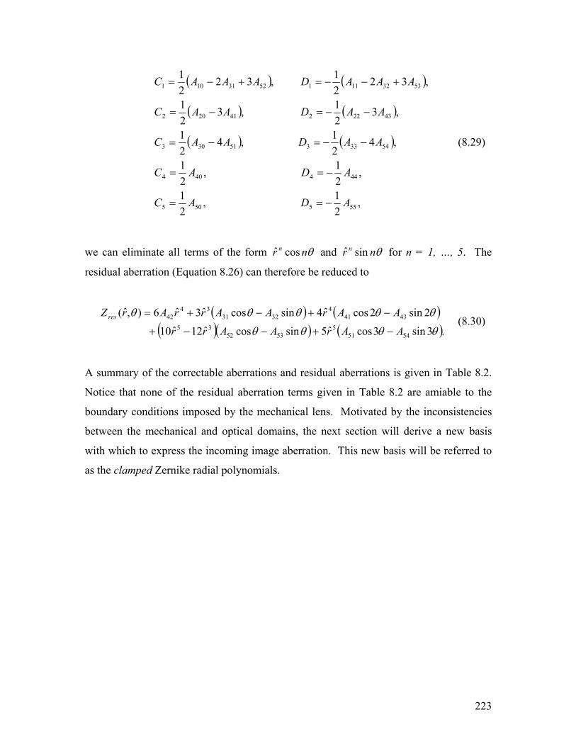
223

( ) ( )

( ) ( )

( ) ( )

,21,

21

,21,

21

,421,4

21

,321,3

21

,3221,32

21

555505

444404

5433351303

4322241202

53321115231101

ADAC

ADAC

AADAAC

AADAAC

AAADAAAC

−==

−==

−−=−=

−−=−=

+−−=+−=

(8.29)

we can eliminate all terms of the form θnr n cosˆ and θnr n sinˆ for n = 1, …, 5. The

residual aberration (Equation 8.26) can therefore be reduced to

( ) ( )

( )( ) ( ).3sin3cosˆ5sincosˆ12ˆ10

2sin2cosˆ4sincosˆ3ˆ6),ˆ(

54515

535235

43414

323134

42

θθθθ

θθθθθ

AArAArr

AArAArrArZ res

−+−−+

−+−+= (8.30)

A summary of the correctable aberrations and residual aberrations is given in Table 8.2.

Notice that none of the residual aberration terms given in Table 8.2 are amiable to the

boundary conditions imposed by the mechanical lens. Motivated by the inconsistencies

between the mechanical and optical domains, the next section will derive a new basis

with which to express the incoming image aberration. This new basis will be referred to

as the clamped Zernike radial polynomials.

224

Table 8.2. Summary of wavefront correction for a membrane optic using uniform

pressure difference (across the outer and inner surfaces of the membrane) and

boundary displacement.

Zernike Polynomial Correctable Portion Residual Aberration

1 1 0

θsinr θsinr 0

θcosr θcosr 0

θ2sinˆ2r θ2sinˆ2r 0

1ˆ2 2 −r 1ˆ2 2 −r 0

θ2cosˆ2r θ2cosˆ2r 0


( ) θsinˆ2ˆ3 3 rr − θsinˆ2r− θsinˆ3 3r

( ) θcosˆ2ˆ3 3 rr − θcosˆ2r− θcosˆ3 3r



( ) θ2sinˆ3ˆ4 24 rr − θ2sinˆ3 2r− θ2sinˆ4 4r

1ˆ6ˆ6 24 +− rr 1ˆ6 2 +− r 4ˆ6r

( ) θ2cosˆ3ˆ4 24 rr − θ2cosˆ3 2r− θ2cosˆ4 4r



( ) θ3sinˆ4ˆ5 35 rr − θ3sinˆ4 3r− θ3sinˆ5 5r

( ) θsinˆ3ˆ12ˆ10 35 rrr +− θsinˆ3r ( ) θsinˆ12ˆ10 35 rr −

( ) θcosˆ3ˆ12ˆ10 35 rrr +− θcosr ( ) θcosˆ12ˆ10 35 rr −

( ) θ3cosˆ4ˆ5 35 rr − θ3cosˆ4 3r− θ3cosˆ5 5r


225

8.5 A Novel Transformation for Describing Image Aberrations

As previously mentioned, the mismatch between the mechanical and optical domains of

the deformable membrane mirror poses a challenge. The following subsections will

describe a novel basis with which to express the Zernike polynomials that is more

suitable to the mechanical properties of the membrane lens.

First, we will define the clamped Zernike radial polynomials, and then we will apply this

new set of polynomials to our static aberration correction analysis. A comparison

between the residual aberrations from our previous analysis with the clamped Zernike

radial polynomials analysis will demonstrate a significant advantage of using the newly

proposed basis. Finally, we will look at possible methods of control based on the newly

defined clamped residuals.

8.5.1 Definition of the Clamped Zernike Radial Polynomials

In this section, we will cast the wavefront aberration in terms of the dynamical mode

shapes of a clamped circular membrane. In doing so, we will define a novel basis of

clamped radial polynomials. Let us define the image aberration radial polynomial as:

mnmn

nmnmnmn

nmn

n rCrrRR 222222 ˆˆˆ −−−−−− +≡+−≡ , (8.31)

where the clamped radial polynomials are defined as:

2,ˆ)ˆ( 222 >−≡ −−− mrrRC mnmnn

mnn , (8.32)

which vanish at both r = 0 and at r = 1. This basis is advantageous to use as it has the

same boundary conditions as the clamped membrane. This advantage will be exploited

subsequently. Following the definition of Equation 8.32, we have

.ˆ5ˆ5ˆ,ˆ2ˆ12ˆ10ˆ,ˆ4ˆ4ˆ,ˆ3ˆ3ˆ

,ˆ6ˆ6ˆ

35335

35

35115

15

24224

24

3113

13

24004

04

rrrRCrrrrRC

rrrRCrrrRC

rrrRC

−=−=+−=−=

−=−=−=−=

−=−=

(8.33)

226

Next, we will insert our definition of the clamped Zernike radial polynomials into our

measured wavefront aberration (Equation 8.19), thus yielding:

( ) ( ) ( )( ) ( ) ( )( ) ( ) ( ) ( )( )

.3sin)ˆ(

sin)ˆ(cos)ˆ(3cos)ˆ(2sin)ˆ(

2cos)ˆ(sin)ˆ(cos)ˆ()ˆ(5sinˆ5cosˆ4sinˆ4cosˆ3sinˆ

3cosˆ2sinˆ)2cos(ˆsinˆcosˆˆ2),ˆ(

3554

1553

1552

3551

2443

2441

1332

1331

0442

555

550

444

440

35433

35130

24322

24120

5332115231102

21422100

θ

θθθθ

θθθθ

θθθθ

θθθ

θθθ

rCA

rCArCArCArCA

rCArCArCArCArA

rArArArAA

rAArAArAA

rAAArAAArAAAArZ

−

−++−

+−++−

+−++−

+++−++

++−+++++−=

(8.34)

Now, we wish to derive an expression for the residual wavefront error, as we previously

defined in Equations 8.25 and 8.26. Performing a similar analysis as was performed by

Wilkes (2005), we get the following expression:

( ) ( ) ( )( ) ( ) ( )( ) ( ) ( ) ( )( )

).5sinˆ5cosˆ()4sinˆ2cosˆ(

)3sinˆ3cosˆ()2sinˆ2cosˆ(

)sinˆcosˆ()ˆ1(4

23sin)ˆ(


2cos)ˆ(sin)ˆ(cos)ˆ()ˆ(5sinˆ5cosˆ4sinˆ4cosˆ3sinˆ

3cosˆ2sinˆ)2cos(ˆsinˆcosˆˆ2),ˆ(

55

55

44

44

33

33

22

22

112

2

03554

1553

1552

3551

2443

2441

1332

1331

0442

555

550

444

440

35433

35130

24322

24120

5332115231102

21422100

θθθθ

θθθθ

θθθ

θθθθ

θθθθ

θθθθ

θθθ

θθθ

rDrCrDrC

rDrCrDrC

rDrCrT

paCrCA

rCArCArCArCA

rCArCArCArCArA

rArArArAA

rAArAArAA

rAAArAAArAAAArZres

++++

++++

++−

∆+−−

−++−

+−++−

+−++−

+++−++

++−+++++−=

(8.35)

As before, we see that by setting like power terms equal to each other, the defocus terms

(those proportional to 2r ) can be eliminated by applying a uniform pressure of

212

4 AaTp −=∆ . (8.36)

227

Similarly, the piston (constant) term can be eliminated by rigidly displacing the boundary

( )4221000 21 AAAC ++= . (8.37)

Finally, solving for the remaining unknowns in Equation 8.35, we find that by displacing

the boundary according to the following relations:

( ) ( )

( ) ( )

( ) ( )

,21,

21

,21,

21

,21,

21

,21,

21

,21,

21

555505

444404

5433351303

4322241202

53321115231101

ADAC

ADAC

AADAAC

AADAAC

AAADAAAC

−==

−==

+−=+=

+−=+=

++−=++=

(8.38)

we can eliminate all terms of the form θnr n cosˆ and θnr n sinˆ for n = 1, …, 5. The

residual aberration (Equation 8.35) can therefore be reduced to

.3sin)ˆ(


2cos)ˆ(sin)ˆ()cos()ˆ()ˆ(),ˆ(

3554

1553

1552

3551

2443

2441

1332

1331

0442

θ

θθθθ

θθθθ

rCA

rCArCArCArCA

rCArCArCArCArZ res

−

−++−

+−+=

(8.39)

Due to our definition of the novel clamped Zernike radial polynomials, the residual

aberration is proportional to the mode shapes of a clamped circular membrane. Table 8.3

summarizes the residuals from the previous traditional Zernike analysis as well as the

current clamped Zernike analysis.

228

Table 8.3. Summary of the residual wavefront aberrations using only uniform

pressure and boundary control as expressed using traditional Zernike radial

polynomials and the proposed clamped Zernike radial polynomials.

Zernike Polynomial Residual Aberration

Traditional Zernike Radial

Residual Aberration

Clamped Zernike Radial

( ) θsinˆ2ˆ3 3 rr − θsinˆ3 3r ( ) θsinˆˆ3 3 rr −

( ) θcosˆ2ˆ3 3 rr − θcosˆ3 3r ( ) θcosˆˆ3 3 rr −

( ) θ2sinˆ3ˆ4 24 rr − θ2sinˆ4 4r ( ) θ2sinˆˆ4 24 rr −

1ˆ6ˆ6 24 +− rr 4ˆ6r ( )24 ˆˆ6 rr −

( ) θ2cosˆ3ˆ4 24 rr − θ2cosˆ4 4r ( ) θ2cosˆˆ4 24 rr −

( ) θ3sinˆ4ˆ5 35 rr − θ3sinˆ5 5r ( ) θ3sinˆˆ5 35 rr −

( ) θsinˆ3ˆ12ˆ10 35 rrr +− ( ) θsinˆ12ˆ10 35 rr − ( ) θsinˆ2ˆ12ˆ10 35 rrr +−

( ) θcosˆ3ˆ12ˆ10 35 rrr +− ( ) θcosˆ12ˆ10 35 rr − ( ) θcosˆ2ˆ12ˆ10 35 rrr +−

( ) θ3cosˆ4ˆ5 35 rr − θ3cosˆ5 5r ( ) θ3cosˆˆ5 35 rr −

To highlight the benefit of the proposed clamped Zernike radial expressions, Figures 8.2

– 8.5 plot the two residual expressions against each other. In the comparison plots, the

sine and cosine terms have been set to unity, plotting the 2-D slice of each residual term

along its angular line of maximum amplitude.

229

Figure 8.2. Comparison between the clamped Zernike polynomial residual )ˆ(13 rC

and the corresponding traditional Zernike residual.

Figure 8.3. Comparison between the clamped Zernike polynomial residual

)ˆ(24 rC and the corresponding traditional Zernike residual.

230





231

8.5.2 Fourier Analysis of the Clamped Zernike Radial Polynomials

Up until this point in our analysis, we have assumed that only a uniform pressure and

boundary control were available for image compensation control. Now we will relax this

assumption and express the optically clamped Zernike radial polynomials in the

mechanical domain of the membrane lens.

Given the clamped Zernike radial polynomials, denoted mnnC 2− , describing the residual

wavefront aberration, we wish to find the Fourier expansion approximation of the

clamped Zernike shape functions using the basis formed by the mode shapes of a

clamped circular membrane, denotedΨ . Our Fourier expansion begins by assuming that,

given the orthonormal basis formed by the mode shapes nψ and the functions mnnC 2−

living in the same Hilbert space, the function mnnC 2− can be expressed as the Fourier

series:

......2211002 +++++=−

iimn

n zzzzC ψψψψ . (8.40)

We wish to find the constants zn, otherwise known as the Fourier coefficients of mnnC 2−

with respect to the basisΨ (Tolstov, 1962). To calculate the Fourier coefficients, we

multiply Equation 8.40 by nψ and assume that the resulting series can be integrated term

by term over the entire membrane domain, Ω. Doing so, we have:

...),2,1(22 =Ω∫=Ω∫ΩΩ

− idzdC iiimn

n ψψ . (8.41)

Solving for the Fourier coefficients, we get:

2

2

2

2

i

imn

n

i

imn

n

i

dC

d

dCz

ψ

ψ

ψ

ψ ∫ Ω=

∫ Ω

∫ Ω= Ω

−

Ω

Ω

−

. (8.42)

232

Equations 8.40-8.42 assume equality, but such equality can only hold if an infinite

number of basis functions are available. Since we do not have an infinite number of basis

functions available, we will have to truncate our analysis and form the best

approximation we can using a limited number of terms. We define the approximated

clamped Zernike residual wavefront aberration as

NNN zzzzC ψψψψ ++++= ...221100 . (8.43)

Further, note that since our basis Ψ was defined to be orthonormal previously, the norm

appearing in Equation 8.42 is equal to unity. Substituting accordingly, we find that

∫ Ω=Ω

− dCz imn

ni ψ2 . (8.44)

8.5.3 Example Fourier Expansion of the Clamped Zernike Radial Polynomials

Having defined our Fourier coefficients in Equation 8.44, we will now apply this

expansion to the residual aberrations described using the clamped Zernike radial

polynomials, as given explicitly in Table 8.3. We will form our modal basis from the

first 36 mode shapes of the clamped membrane, including both symmetric and

asymmetric modes. Further, we will only take the theta dependent mode shapes that are

functions of sine and use them as a basis for the clamped Zernike radial polynomials that

are also a function of sine and / or r . We could also take the cosine terms in our

analysis, but since they are orthogonal to the clamped Zernike radial polynomials, the

integration term by term would give trivial solutions.

Now we will focus our analysis on the following residual aberration

terms: 04C , θsin1

3C , θ2sin24C , θsin1

5C , and θ3sin35C . Following through with the

integration scheme stated in Equation 8.44 we get the following non-trivial terms:

233

.0002.00462.00768.0...1411.02986.07622.05894.0sin

,0174.00274.00470.00910.02156.07721.03sin

,0128.00208.00372.00767.02017.08883.02sin

,0080.00135.00254.00571.01742.00694.1sin

,0425.00748.01497.03659.02518.14276.1

561615

1413121115

36353433323135

26252423222124

16151413121113

06050403020104

sss

ssss

ssssss

ssssss

ssssss

C

C

C

C

C

ψψψψψψψθ

ψψψψψψθ

ψψψψψψθ

ψψψψψψθ

ψψψψψψ

−−−−−−−≈

−−−−−−≈

−−−−−−≈

−−−−−−≈

−−−−−−≈

(8.45)

To further exhibit the excellent match between the modal expansion and the original

residual aberration, Figures 8.6 – 8.10 plot the original residual, the projected residual,

and the error between the two. In each of the plots, the residual aberrations have been

normalized by their largest respective magnitude.

234

Figure 8.6. Comparison between the θsin13C residual term (top left) and its

modal projection (top right) and the error between the two spaces (bottom).

235

Figure 8.7. Comparison between the θ2sin24C residual term (top left) and its


236

Figure 8.8. Comparison between the 04C residual term (top left) and its modal

projection (top right) and the error between the two spaces (bottom).

237

Figure 8.9. Comparison between the θ3sin35C residual term (top left) and its


238

Figure 8.10. Comparison between the θsin15C residual term (top left) and its


239

Figures 8.6 – 8.10 demonstrate a useful mapping between the optical and mechanical

worlds. By transforming a known incoming image aberration into two parts, a portion

that can be corrected using uniform actuation pressure on the backside of the membrane

lens and a portion that can be corrected using a distributed actuation pressure, we have

shown that the deformable face of a membrane mirror can be used as a nearly 100%

effective optic. The novel clamped Zernike radial polynomials provide a means for

translating the incoming aberration into the two mentioned portions while simultaneously

describing the necessary pressure distribution and magnitude for effective adaptive optic

control. A proposed control scheme will be discussed in the future works section of the

next chapter.

8.6 Chapter Summary

In the present chapter, we have developed a novel basis for conversing between the

optical and mechanical worlds. The analysis performed has demonstrated that the

structural characteristics of a circular membrane lens can be used advantageously as an

advanced adaptive optic deformable mirror for eliminating nearly 100% of a 5th order

image aberration.

The proposed basis transformation has been described as the clamped Zernike radial

polynomials. The clamped Zernike radial polynomials differ from traditional Zernike

polynomials in that they have zero displacement at the boundary of the described image

aberration. Consequently, the image aberration can be divided into two parts. The first

portion of the aberration can be corrected by applying a uniform pressure on the backside

of the membrane and via continuous deformation control of the boundary. The remaining

residual portion requires a distributed actuation on the backside of the membrane.

However, through the use of the clamped Zernike radial polynomials, the remaining

residual is zero along the edge of the membrane—a conformable transformation to the

structural configuration of the lens. Consequently, the distributed pressure necessary to

eliminate the residual aberration can be easily transformed via a Fourier analysis into a

modal summation based on the modes of a clamped circular membrane. Such a mapping

240

is key for describing the necessary form of actuation for making a 100% effective

deformable membrane optic a reality in the near future.

chapter 8: the clamped zernike radial polynomials

Documents