chapter 9. air quality and public health
TRANSCRIPT

Chapter 9. Air Quality and Public Health FINAL REPORT: LA100—The Los Angeles 100% Renewable Energy Study
March 2021
maps.nrel.gov/la100

FINAL REPORT: The Los Angeles 100% Renewable Energy Study
Chapter 9. Air Quality and Public Health March 2021
Lead Author of Chapter 9: Garvin Heath1
Air Quality Modeling: George Ban-Weiss,2 Yun Li,2 Jiachen Zhang,2 Vikram Ravi1
Public Health and Monetization: Vikram Ravi1 1 National Renewable Energy Laboratory 2 University of Southern California
Suggested Citation—Entire Report Cochran, Jaquelin, and Paul Denholm, eds. 2021. The Los Angeles 100% Renewable Energy Study. Golden, CO: National Renewable Energy Laboratory. NREL/TP-6A20-79444. https://maps.nrel.gov/la100/.
Suggested Citation—Chapter 9 Heath, Garvin, George Ban-Weiss, Vikram Ravi, Yun Li, and Jiachen Zhang. 2021. “Chapter 9: Air Quality and Public Health.” In The Los Angeles 100% Renewable Energy Study, edited by Jaquelin Cochran and Paul Denholm. Golden, CO: National Renewable Energy Laboratory. NREL/TP-6A20-79444-9. https://www.nrel.gov/docs/fy21osti/79444-9.pdf.

Produced under direction of the Los Angeles Department of Water and Power by the National Renewable Energy Laboratory (NREL) under ACT Agreement 18-39, LADWP Ref: 47481.
NOTICE This work was authored, in part, by the National Renewable Energy Laboratory (NREL), operated by Alliance for Sustainable Energy, LLC, for the U.S. Department of Energy (DOE) under Contract No. DE-AC36-08GO28308. Support for the work was provided by the Los Angeles Department of Water and Power under ACT Agreement 18-39, LADWP Ref: 47481. The views expressed in the article do not necessarily represent the views of the DOE or the U.S. Government. The U.S. Government retains and the publisher, by accepting the article for publication, acknowledges that the U.S. Government retains a nonexclusive, paid-up, irrevocable, worldwide license to publish or reproduce the published form of this work, or allow others to do so, for U.S. Government purposes.
This report is available at no cost from the National Renewable Energy Laboratory (NREL) at www.nrel.gov/publications.
U.S. Department of Energy (DOE) reports produced after 1991 and a growing number of pre-1991 documents are available free via www.OSTI.gov.
Cover photo from iStock 596040774.
NREL prints on paper that contains recycled content.

Chapter 9. Air Quality and Public Health
LA100: The Los Angeles 100% Renewable Energy Study Chapter 9, page iii
Context The Los Angeles 100% Renewable Energy Study (LA100) is presented as a collection of 12 chapters and an executive summary, each of which is available as an individual download.
• The Executive Summary describes the study and scenarios, explores the high-level findings that span the study, and summarizes key findings from each chapter.
• Chapter 1: Introduction introduces the study and acknowledges those who contributed to it. • Chapter 2: Study Approach describes the study approach, including the modeling
framework and scenarios. • Chapter 3: Electricity Demand Projections explores how electricity is consumed by
customers now, how that might change through 2045, and potential opportunities to better align electricity demand and supply.
• Chapter 4: Customer-Adopted Rooftop Solar and Storage explores the technical and economic potential for rooftop solar in LA, and how much solar and storage might be adopted by customers.
• Chapter 5: Utility Options for Local Solar and Storage identifies and ranks locations for utility-scale solar (ground-mount, parking canopy, and floating) and storage, and associated costs for integrating these assets into the distribution system.
• Chapter 6: Renewable Energy Investments and Operations explores pathways to 100% renewable electricity, describing the types of generation resources added, their costs, and how the systems maintain sufficient resources to serve customer demand, including resource adequacy and transmission reliability.
• Chapter 7: Distribution System Analysis summarizes the growth in distribution-connected energy resources and provides a detailed review of impacts to the distribution grid of growth in customer electricity demand, solar, and storage, as well as required distribution grid upgrades and associated costs.
• Chapter 8: Greenhouse Gas Emissions summarizes greenhouse gas emissions from power, buildings, and transportation sectors, along with the potential costs of those emissions.
• Chapter 9: Air Quality and Public Health (this chapter) summarizes changes to air quality (fine particulate matter and ozone) and public health (premature mortality, emergency room visits due to asthma, and hospital admissions due to cardiovascular diseases), and the potential economic value of public health benefits.
• Chapter 10: Environmental Justice explores implications for environmental justice, including procedural and distributional justice, with an in-depth review of how projections for customer rooftop solar and health benefits vary by census tract.
• Chapter 11: Economic Impacts and Jobs reviews economic impacts, including local net economic impacts and gross workforce impacts.
• Chapter 12: Synthesis reviews high-level findings, costs, benefits, and lessons learned from integrating this diverse suite of models and conducting a high-fidelity 100% renewable energy study.

Chapter 9. Air Quality and Public Health
LA100: The Los Angeles 100% Renewable Energy Study Chapter 9, page iv
Table of Contents Key Findings ................................................................................................................................................ 1 1 Introduction ......................................................................................................................................... 10 2 Methodology and Data ....................................................................................................................... 13
2.1 Air Quality Modeling .................................................................................................................. 13 2.1.1 General Description of Air Quality Modeling ............................................................... 13 2.1.2 Model Selection and Justification .................................................................................. 13 2.1.3 Model Domain and Time Period .................................................................................... 13 2.1.4 Scenarios for Analysis .................................................................................................... 15 2.1.5 Emission Inventory Development .................................................................................. 17 2.1.6 Analysis Techniques for Air Pollutant Concentrations .................................................. 24
2.2 Methods for Health Impacts Modeling: Estimation of Mortality and Morbidity Changes ......... 25 2.2.1 From Epidemiology to Health Impacts Modeling .......................................................... 25 2.2.2 Health Impacts Modeling Using BenMAP .................................................................... 25 2.2.3 Estimating Exposed Population (pop) ............................................................................ 27 2.2.4 Predicted Changes in Air Quality (∆C) .......................................................................... 28 2.2.5 Baseline Incidence Data (YO) ......................................................................................... 29 2.2.6 Selecting Effect Estimates (β) ........................................................................................ 29
2.3 Methods for Monetization of Benefits ........................................................................................ 30 2.3.1 Monetization of Air Quality Health Effects ................................................................... 30 2.3.2 Methods for Monetizing Morbidity ................................................................................ 31 2.3.3 Methods for Monetizing Mortality ................................................................................. 31
3 Results and Discussion ..................................................................................................................... 34 3.1 Air Quality................................................................................................................................... 34
3.1.1 Emission Inventory for Baseline and Future Scenarios ................................................. 34 3.1.2 Simulated Air Quality for Baseline and Future Scenarios ............................................. 39
3.2 Public Health ............................................................................................................................... 49 3.2.1 Health Benefits Associated with Air Quality Changes in 2045 ..................................... 50
3.3 Monetization of Health Benefits ................................................................................................. 60 4 Conclusion .......................................................................................................................................... 63
4.1 Air Quality................................................................................................................................... 63 4.2 Public Health Benefits and their Monetization ........................................................................... 64
5 Important Caveats .............................................................................................................................. 66 6 References .......................................................................................................................................... 69 Appendix A. Qualitative Analysis of Electrified Medium- and Heavy-Duty Vehicles .................. 75
A.1 Transportation and Technology Adoption .................................................................................. 75 A.2 Electric Distribution System Impacts .......................................................................................... 80 A.3 Bulk Power System Impacts ....................................................................................................... 81 A.4 Greenhouse Gas Emissions Impacts ............................................................................................ 82 A.5 Air Quality and Health Benefits .................................................................................................. 83 A.6 Environmental Justice Implications ............................................................................................ 95 A.7 GHG Emissions Benefits ............................................................................................................ 96 A.8 References ................................................................................................................................... 96 A.9 Supplemental Information ........................................................................................................... 99
Appendix B. Additional Information on Methods and Results for Air Quality Analysis ........... 101 B.1 Additional Information on Model Configuration ...................................................................... 101 B.2 Model Evaluation of Simulated O3 and PM2.5 Concentrations with Historical Observations ... 102 B.3 Explanation on Raw Emissions Used for Emission Projections ............................................... 103 B.4 Site-Specific Emission Factors for LADWP-Owned Power Plants Applied to Emission
Projection in the SB100 and Early & No Biofuels Scenarios ................................................... 103 B.5 Scaling Factors Used for Projection of Transportation Emission Sources ................................ 104

Chapter 9. Air Quality and Public Health
LA100: The Los Angeles 100% Renewable Energy Study Chapter 9, page v
B.6 Scaling Factors Used for Projection of Emissions from Commercial and Residential Buildings ................................................................................................................................... 104
B.7 Emission Inventories for NOx and PM2.5 in Los Angeles from all Anthropogenic Sources for the Selected LA100 Scenarios ............................................................................................. 105
B.8 Emission Inventories for CO, SOx, VOC, and NH3 from LA100-Influenced Sectors in Los Angeles for the Selected LA100 Scenarios ........................................................................ 107
B.9 Comparison of Simulated O3 and PM2.5 Concentrations among Baseline (2012), SB100 – Moderate, and Early & No Biofuels – High for Los Angeles ................................................... 115
B.10 Comparison of Simulated O3 and PM2.5 Concentration among Selected Future LA100 scenarios for the Innermost Model Domain .............................................................................. 116
Appendix C. Additional Results for Health Analysis .................................................................... 118 C.1 Effects of Changing Air Quality from Various LA100 Scenarios on Cardiovascular
Hospital Admissions and Heart Attacks .................................................................................... 118 C.2 Health Incidences Aggregated at the District Level .................................................................. 122 C.3 Health Incidences Aggregated at the County Level .................................................................. 125 C.4 Valuation of Health Benefits ..................................................................................................... 133

Chapter 9. Air Quality and Public Health
LA100: The Los Angeles 100% Renewable Energy Study Chapter 9, page vi
List of Figures Figure 1. Contribution of LA100-influenced sectors to annual average emissions in Los Angeles in
2045 compared to 2012 Baseline ............................................................................................. 2 Figure 2. Spatial pattern of simulated July daily maximum 8-hour average ozone concentrations in
Los Angeles for (a) 2012 Baseline and (b) comparison between SB100 – Moderate and the 2012 Baseline ..................................................................................................................... 5
Figure 3. Overview of how this chapter, Chapter 9, relates to other components of LA100 ...................... 12 Figure 4. Three two-way nested domains used for all simulations ............................................................. 14 Figure 5. Schematic showing the approach used in BenMAP for calculating changes in health impacts
incidences (∆Y) due to a change in pollutant concentration by ∆C. ...................................... 27 Figure 6. Total population per modeling grid cell for the LA100 WRF-Chem modeling domain (left)
and the LADWP service territory (right) ............................................................................... 28 Figure 7. Approach for monetizing morbidity used in BenMAP ................................................................ 31 Figure 8. Approach for monetizing mortality in BenMAP ......................................................................... 32 Figure 9. Annually averaged daily NOx emissions from LA100-influenced sources in Los Angeles
for all selected scenarios ........................................................................................................ 35 Figure 10. Annually averaged daily PM2.5 emissions from LA100-influenced sources in Los Angeles
for all selected scenarios ........................................................................................................ 38 Figure 11. O3 isopleth diagram to illustrate how 8-hour O3 concentration design values (DV) at a
location in Los Angeles can change in response to decreases in NOx and VOC emissions (in units of tons per day) ........................................................................................................ 42
Figure 12. Spatial pattern of simulated July daily maximum 8-hour average O3 concentrations in Los Angeles for (a) Baseline (2012), and (b) SB100 – Moderate minus Baseline (2012) ..... 43
Figure 13. Spatial pattern of simulated July daily maximum 8-hour average O3 in Los Angeles for (a) SB100 – Moderate, and differences between SB100 – Moderate and (b) SB100 – High, (c) Early & No Biofuels – Moderate, and (d) Early & No Biofuels – High ................ 44
Figure 14. Spatial pattern of PM2.5 concentrations in Los Angeles for (a) Baseline (2012), and (b) SB100 – Moderate minus Baseline (2012) ....................................................................... 46
Figure 15. Spatial pattern of simulated PM2.5 concentrations in Los Angeles for (a) SB100 – Moderate, and differences between SB100 – Moderate and (b) SB100 – High, (c) Early & No Biofuels – Moderate, and (d) Early & No Biofuels – High .......................... 47
Figure 16. Contributions to citywide annual average PM2.5 concentrations (µg/m3) by species for all selected scenarios .............................................................................................................. 48
Figure 17. Fifteen LA districts annotated by district number (left) ............................................................ 50 Figure 18. Health benefits due to air quality changes from the SB100 – Moderate to the Early &
No Biofuels – Moderate scenario are shown by avoided mortality (A) and ER visits (B) .... 51 Figure 19. Health benefits due to air quality changes from the SB100 – High to the Early & No
Biofuels – High scenario ........................................................................................................ 52 Figure 20. Impacts of concentration change from SB100 – Moderate to SB100 – High scenario on
avoided incidences of mortality (A) and ER visits (B) from changes in PM2.5 and O3 concentration at the district level ........................................................................................... 53
Figure 21. Impacts of concentration change from the Early & No Biofuels – Moderate to Early & No Biofuels – High scenario on avoided incidences of mortality (A) and ER visits (B) from changes in annual average PM2.5 and summertime O3 concentration for the 15 LA city council districts ...................................................................................................................... 54
Figure 22. Avoided mortality incidences (A) and asthma ER visits (B) from a reduction in concentration of PM2.5 and O3 in the Early & No Biofuels – High scenario compared to SB100 – Moderate ................................................................................................................. 55
Chapter 9. Air Quality and Public Health
LA100: The Los Angeles 100% Renewable Energy Study Chapter 9, page vii
Figure 23. Changes in health impacts due to PM2.5 and O3 concentration changes in the SB100 – Moderate scenario in 2045 compared to the Baseline in 2012, shown here for avoided mortality (A) and asthma caused ER visits (B) ...................................................................... 57
Figure 24. Changes in health impacts due to PM2.5 and O3 concentration changes in the Early & No Biofuels – High scenario in 2045 compared to the 2012 baseline, shown here for avoided mortality (A) and asthma caused ER visits (B) ...................................................................... 58
Figure 25. Monetized health benefits (in 2019 U.S. dollars) for the 15 LA City Council districts across the LA100 scenarios compared ................................................................................... 60
Figure 26. U.S. transportation energy use by mode, 2019 .......................................................................... 76 Figure 27. Relative contribution of medium-duty, heavy-duty, and all other vehicle categories to
the total VMT, and emissions of selected pollutants for 2020 and 2045 in Los Angeles ...... 85 Figure 28. Projected changes in the emissions of various pollutants for medium-duty, heavy-duty,
and all other vehicle categories between 2020 and 2045 in Los Angeles .............................. 86 Figure 29. Contribution of various emission processes to total PM2.5 emissions in 2020 and 2045
for MHDVs ............................................................................................................................ 94 Figure 30. Example of O3 isopleth diagram and effect of NOx and VOC changes on O3
concentration ........................................................................................................................ 100 Figure 31. Annually averaged daily NOx emissions from all anthropogenic sources in Los Angeles
for all selected scenarios ...................................................................................................... 105 Figure 32. Annually averaged daily PM2.5 emissions from all anthropogenic sources in Los Angeles
for all selected scenarios ...................................................................................................... 106 Figure 33. Annually averaged daily CO emissions from LA100-influenced sources in Los Angeles
for all selected scenarios ...................................................................................................... 107 Figure 34. Annually averaged daily SOx emissions from LA100-influenced sources in Los Angeles
for all selected scenarios ...................................................................................................... 109 Figure 35. Annually averaged daily VOC emissions from LA100-influenced sources in Los Angeles
for all selected scenarios ...................................................................................................... 111 Figure 36. Annually averaged daily NH3 emissions from LA100-influenced sources in Los Angeles
for all selected scenarios ...................................................................................................... 113 Figure 37. Spatial pattern of simulated July daily maximum 8-hour average O3 concentrations in
Los Angeles for (a) Baseline (2012), (b) SB100 – Moderate minus Baseline (2012), and (c) Early & No Biofuels – High minus Baseline (2012) ...................................................... 115
Figure 38. Spatial pattern of PM2.5 concentrations in Los Angeles for (a) Baseline (2012), (b) SB100 – Moderate minus Baseline (2012), and (c) Early & No Biofuels – High minus Baseline (2012) ......................................................................................................... 115
Figure 39. Spatial pattern of simulated July daily maximum 8-hour average O3 in the innermost model domain for (a) SB100 – Moderate, and differences between SB100 – Moderate and (b) SB100 – High, (c) Early & No Biofuels – Moderate, and (d) Early & No Biofuels – High .................................................................................................................... 116
Figure 40. Spatial pattern of simulated PM2.5 concentrations in the innermost model domain for (a) SB100 – Moderate, and differences between SB100 – Moderate and (b) SB100 – High, (c) Early & No Biofuels – Moderate, and (d) Early & No Biofuels – High .............. 117
Figure 41. Change in incidences of cardiovascular hospital admissions in Los Angeles for various scenarios compared .............................................................................................................. 120
Figure 42. Change in incidences of heart attacks (AMI) in Los Angeles for various scenarios compared .............................................................................................................................. 121
Figure 43. County-level changes in the mortality incidences in 2045 from various LA100 scenario comparisons ......................................................................................................................... 125
Figure 44. County-level changes in asthma-related ER visits in 2045 from various LA100 scenario comparisons ........................................................................................................... 127

Chapter 9. Air Quality and Public Health
LA100: The Los Angeles 100% Renewable Energy Study Chapter 9, page viii
Figure 45. Net change in hospital admissions (all cardiovascular, less myocardial) at county level from various scenario compared in 2045 ............................................................................. 129
Figure 46. Net change in heart attacks (acute myocardial infarctions) at county level from various scenario compared in 2045................................................................................................... 131
List of Tables Table 1. Annually Averaged Daily NOx Emissions (metric tons/day) from LA100-Influenced Sources
in Los Angeles for Evaluated Scenarios .................................................................................. 3 Table 2. Annually Averaged Daily PM2.5 Emissions (metric tons/day) from LA100-Influenced Sources
in Los Angeles for Evaluated Scenarios .................................................................................. 3 Table 3. Simulated Los Angeles Citywide Spatial Average of Daily Maximum 8-hour Average Ozone
in July and Annual Average Daily PM2.5 for Evaluated LA100 Scenarios .............................. 5 Table 4. Selected Health Benefits (Avoided Deaths) from Evaluated LA100 Scenarios and
Total Monetized Benefits (from all Evaluated Health Effects) ................................................ 7 Table 5. Scenario Names and Key Assumptions Used for Analyzing Air Pollutant Emissions and Air
Quality Co-Benefits ............................................................................................................... 16 Table 6. Fraction of Light-Duty Vehicles and Buses That Are Assumed to Be Electric Powered in
2045 for Moderate and High Electrification Levels ............................................................... 17 Table 7. Fraction of Buildings/Households by End Use That Are Assumed to Be Electric Powered in
2045 for Moderate and High Electrification .......................................................................... 17 Table 8. Fraction of Port Sources That Are Assumed to Be Electric Powered in 2045 for both
Moderate and High Electrification in the Air Quality Analysisa ........................................... 17 Table 9. Available Health Endpoints That Can Be Modeled Using BenMAP ........................................... 26 Table 10. Baseline Incidence Data Available for the Model Domain ........................................................ 29 Table 11. Mortality and Morbidity HIF Used ............................................................................................. 30 Table 12. Available Mortality and Morbidity Valuation Functions in BenMAP ....................................... 33 Table 13. Annually Averaged Daily NOx Emissions (metric tons/day) from LA100-Influenced
Sources in Los Angeles and Citywide Total Emissions for all Selected Scenarios ............... 36 Table 14. Annual Total NOx Emissions (metric tons/year) Generated from LADWP-Owned Power
Plants Located in the South Coast Air Basin by Fuel Technology Types ............................. 37 Table 15. Annually Averaged Daily PM2.5 Emissions (metric tons/day) from LA100-Influenced
Sources and Citywide Total Emissions in Los Angeles for all Selected Scenarios ............... 39 Table 16. Simulated Spatial Average (over City of Los Angeles) Daily Maximum 8-hour Average O3
in July for all Selected Scenarios ........................................................................................... 41 Table 17. Simulated PM2.5 Concentrations for all Selected Scenarios Averaged over the City of Los
Angeles and the Four Simulated Months ............................................................................... 46 Table 18. Avoided Incidences of All-Cause Mortality from the Seven Scenarios Compared .................... 59 Table 19. Valuation of Annual Health Benefits from the Six Scenarios Compared (in $ Million, in
2019 U.S. dollars) .................................................................................................................. 62 Table 20. Vehicle Classification Defining Medium- and Heavy-Duty Vehicles Used Here ...................... 84 Table 21. Summary of Literature that Estimates Emissions and Air Quality Benefits from Various
Electrification Scenarios, including Medium- and Heavy-Duty Vehicle Electrification ....... 88 Table 22. Summary of Literature that Estimates Health Benefits from Various Electrification
Scenarios, including Medium- and Heavy-Duty Vehicle Electrification ............................... 92 Table 23. National Ambient Air Quality Standard for the Six Criteria Pollutants ..................................... 99 Table 24. Statistics of Model Evaluationa ................................................................................................. 102 Table 25. Recommended Benchmarks of Statistical for Model Evaluation of Air Pollutant ................... 103 Table 26. Emission Factors Used in the SB100 Scenario ......................................................................... 103 Table 27. Emission Factors Used in the Early & No Biofuels Scenario ................................................... 104

Chapter 9. Air Quality and Public Health
LA100: The Los Angeles 100% Renewable Energy Study Chapter 9, page ix
Table 28. Scaling Factors of Fuel Consumption in Commercial Buildings from 2020 to 2045 under Moderate and High Electrification Assumptions ................................................................. 104
Table 29. Scaling Factors of Fuel Consumption in Residential Buildings from 2020 to 2045 under Moderate and High Electrification Assumptions ................................................................. 105
Table 30. Annually Averaged Daily CO Emissions (metric tons/day) from LA100-Influenced Sources in Los Angeles and Citywide Total Emissions for all Selected Scenarios ............. 108
Table 31. Annually Averaged Daily SOx Emissions (metric tons/day) from LA100-Influenced Sources in Los Angeles and Citywide Total Emissions for all Selected Scenarios ............. 110
Table 32. Annually Averaged Daily VOC Emissions (metric tons/day) from LA100-Influenced Sources in Los Angeles and Citywide Total Emissions for all Selected Scenarios ............. 112
Table 33. Annually Averaged Daily NH3 Emissions (metric tons/day) from LA100-Influenced Sources in Los Angeles and Citywide Total Emissions for all Selected Scenarios ............. 114
Table 34. Incidence Changes for Asthma-Caused ER Visits in 15 LA Districts for the Seven LA100 Scenarios Compared ............................................................................................................ 122
Table 35. Incidence Changes for all Cardiovascular (Less Myocardial) Hospital Admission in 15 LA Districts for the Seven LA100 Scenarios Compared ..................................................... 123
Table 36. Incidence Changes for Heart Attacks (Acute Myocardial Infarctions) in the 15 LA Districts for the Seven LA100 Scenarios Compared .......................................................................... 124
Table 37. Avoided Incidences of All-Cause Mortality from the Seven LA100 Scenarios Compared for the Counties Wholly and Partially Within the Modeling Domain ................................. 126
Table 38. Incidence Changes for Asthma-Related ER Visits in Counties Within the Modeling Domain for the Seven LA100 Scenarios Compared ............................................................ 128
Table 39. Incidence Changes for Cardiovascular Hospital Admission in Counties Within the Modeling Domain for the Seven LA100 Scenarios Compared ............................................ 130
Table 40. Incidence Changes for Heart Attacks (Acute Myocardial Infarctions) in Counties Within the Modeling Domain for the Seven LA100 Scenarios Compared ...................................... 132
Table 41. Valuation of Health Benefits from Avoided Mortality and Morbidity for the Seven Scenarios Compared (in $ Million using 2019 U.S. Dollars) at the County Level .............. 133

Chapter 9. Air Quality and Public Health
LA100: The Los Angeles 100% Renewable Energy Study Chapter 9, page 1
Key Findings A key element of the LA100 study is to assess the impacts of different pathways to 100% renewable energy on air quality and subsequent impacts on human health. In this chapter, we assess these impacts using state-of-science atmospheric and health impacts tools. We consider one recent year for a baseline (2012) and four LA100 future scenarios (SB100 – Moderate Load Electrification, SB100 – High Load Electrification, Early & No Biofuels – Moderate Load Electrification, and Early & No Biofuels – High Load Electrification) and quantify the air quality and health effects due to air pollutant emissions reductions from changes in the power sector, changes in electrification of end-use sources, and from combined changes in power sector and end-use electrification in 2045, the final LA100 scenario year. These scenarios and their associated load electrification levels were chosen to enable pairwise comparisons that would isolate the contribution of certain sectors, namely the power sector (when holding electrification level constant) and electrification of end-use sectors (when holding power plant eligibility constant) at the bookends of potential air pollutant emission reductions.
Overall, results suggest that the LA100 scenarios could lead to citywide reductions in major air pollutant emissions including oxides of nitrogen (NOx) and fine particulate matter (PM2.5). The largest reductions in emissions derive from changes to non-power sector sources that are affected by the LA100 scenarios (selected transportation and buildings, as well as the Ports of Los Angeles and Long Beach). These reductions in air pollutant emissions due to LA100 are modeled to consequently lead to citywide reductions in PM2.5 concentration and an increase in ozone (O3) concentration in certain areas within Los Angeles. That ozone concentration increases despite NOx emission reductions can be thought of as temporary “growing pains” that the city experiences on the path toward ozone reductions. Once NOx emissions get sufficiently low, further emission decreases will lead to marked ozone reductions. Health effects are proportional to the concentration changes: where both pollutants contribute to the same health endpoint, the reductions in PM2.5 outweigh the slight increases in ozone. When weighted by the costs of each health effect, the overall changes to air quality from LA100 scenarios could provide hundreds of millions of dollars—and up to nearly $1.5 billion—in monetized benefits in the year 2045.
How do changes due to electrification levels and power plant eligibility in LA100 scenarios affect NOx and PM2.5 emissions? • All selected LA100 scenarios result in significant reductions in annual, primary emissions
(directly emitted) for LA100-influenced sources in Los Angeles in 2045 compared to the 2012 Baseline. SB100 – Moderate (which we use as an LA100 reference scenario for this analysis) leads to an estimated annual reduction in NOx emissions in 2045 of 88% (~45 metric tons/day) and 38% (~1.3 metric tons/day) in PM2.5 emissions compared to 2012 (see Figure 1, Table 1, and Table 2 below), for LA100-influenced sources.1 These reductions are due to changes in the scenarios (i.e., electrification of end-use categories and changes in power plant fuel use and fuel choice), and due to changes occurring outside the scope of LA100 (like the California Air Resources Board’s On-Road Heavy-Duty Diesel Vehicles
1 NOx mass emissions are reported as nitrogen dioxide (NO2)-equivalent, based on the molecular weight of NO2.

Chapter 9. Air Quality and Public Health
LA100: The Los Angeles 100% Renewable Energy Study Chapter 9, page 2
Regulation [SCAQMD, 2017]). Reduced emissions from light-duty vehicles and the Ports are the two major contributors to decreases in LA100-influenced NOx and PM2.5 emissions (as seen in Figure 1).
• Among the LA100 scenarios (all in 2045), Early & No Biofuels – High has the greatest reduction in annual emissions for LA100-influenced sources: for instance, 62% (4.0 metric tons/day) and 39% (0.8 metric tons/day) lower NOx and PM2.5 emissions relative to SB100 – Moderate, respectively. These reductions are due almost entirely to electrification of light-duty vehicles, building appliances and the Ports. Isolating impacts of changes to the power system (both fuel use and fuel type), NOx emissions generated from the in-basin Los Angeles Department of Water and Power (LADWP)-owned power plants are 84%–88% lower in Early & No Biofuels scenarios as compared to SB100 scenarios, when load levels are held constant. No emissions of PM2.5 occur from the power sector in 2045 in Early & No Biofuels because all plants are assumed to burn hydrogen, for which we assume no PM2.5 emissions.
• The emissions from LA100-influenced sources as a fraction of all anthropogenic NOx and PM2.5 emissions in Los Angeles decrease from the 2012 Baseline (which is 34% for NOx and 18% for PM2.5) to the reference scenario in 2045 (10% for NOx and 12% for PM2.5 in SB100 – Moderate, for instance), indicating the potentially smaller contribution of LA100-influnced citywide sources to air pollutant emissions and air quality impacts in the future. The fraction is higher for scenarios with Moderate electrification relative to scenarios with High electrification but is identical for SB100 and Early & No Biofuels with the same electrification level, which suggests the role of electrification outweighs changes to LADWP power plants in citywide emissions.
Figure 1. Contribution of LA100-influenced sectors to annual average emissions in Los Angeles in
2045 compared to 2012 Baseline The percent labels above each column represent the fraction of emissions that are from LA100-influenced sectors out
of the total emissions from all sources in the city. The power sector emissions shown represent LADWP-owned power plants located in the South Coast Air Basin.

Chapter 9. Air Quality and Public Health
LA100: The Los Angeles 100% Renewable Energy Study Chapter 9, page 3
Table 1. Annually Averaged Daily NOx Emissions (metric tons/day) from LA100-Influenced Sources in Los Angeles for Evaluated Scenarios
Percentages in parentheses show the contribution of emissions from an LA100-influenced source to citywide total emissions in a scenario. Future scenarios are projected to year 2045.
Scenario LADWP-Owned Power Plants
The Ports of LA and LB
Residential Buildings
Commercial Buildings LDVs Buses
Baseline (2012) 0.54 (0.4%)
12 (8%)
6.2 (4%)
0.49 (0.3%)
27 (18%)
5.3 (4%)
SB100 – Moderate
0.15 (0.2%)
1.7 (3%)
2.2 (4%)
0.47 (0.8%)
1.8 (3%) 0
SB100 – High 0.15 (0.3%)
1.1 (2%)
0.41 (0.7%)
0.01 (0.02%)
0.88 (2%) 0
Early & No Biofuels – Moderate
0.02 (0.03%)
1.7 (3%)
2.2 (4%)
0.47 (0.8%)
1.8 (3%) 0
Early & No Biofuels – High
0.02 (0.04%)
1.1 (2%)
0.41 (0.7%)
0.01 (0.02%)
0.88 (2%) 0
LA = Los Angeles; LB = Long Beach; LDV = light-duty vehicles
Table 2. Annually Averaged Daily PM2.5 Emissions (metric tons/day) from LA100-Influenced Sources in Los Angeles for Evaluated Scenarios
Percentages in the parentheses show the contribution of emissions from an LA100-influenced source to citywide total emissions in a scenario. Future scenarios are projected to year 2045.
Scenario LADWP-Owned Power Plantsa
The Ports of LA and LB
Residential Buildings
Commercial Buildings LDVs Busesb
Baseline (2012) 0.24 (1%)
0.39 (2%)
0.64 (3%)
0.07 (0.4%)
1.8 (10%)
0.21 (1%)
SB100 – Moderate
0.03 (0.2%)
0.13 (0.8%)
0.38 (2%)
0.09 (0.5%)
1.4 (8%)
0.07 (0.4%)
SB100 – High 0.03 (0.2%)
0.09 (0.6%)
0.07 (0.4%)
0.002 (0.01%)
1.0 (6%)
0.07 (0.4%)
Early & No Biofuels – Moderate
0 0.13 (0.8%)
0.38 (2%)
0.09 (0.5%)
1.4 (8%)
0.07 (0.4%)
Early & No Biofuels – High
0 0.09 (0.6%)
0.07 (0.4%)
0.002 (0.01%)
1.0 (6%)
0.07 (0.4%)
LA = Los Angeles; LB = Long Beach; LDV = light-duty vehicles a LADWP-owned power plants are modeled to combust only hydrogen by 2045 in the Early & No Biofuels scenario, which are assumed to emit no PM2.5. b All buses are assumed to be zero-emission vehicles by 2030, yet brake and tire wear remain as sources of PM2.5 emissions despite no emissions from engines.

Chapter 9. Air Quality and Public Health
LA100: The Los Angeles 100% Renewable Energy Study Chapter 9, page 4
How do changes in emissions in LA100 scenarios in turn affect ozone and PM2.5 concentrations? • Primer: Ozone is a pollutant that is not directly emitted, but rather is formed in the
atmosphere following emissions of “precursor” pollutants, most importantly NOx and a grouping of individual pollutants collectively called volatile organic compounds (VOCs). Fine particulate matter (PM2.5) is both directly emitted and is also formed in the atmosphere (e.g., from NOx, SO2, and VOC precursor emissions following different chemical reaction pathways), the latter being the larger contributor to PM2.5 concentrations in Los Angeles.
• Reductions in the emissions of primary PM2.5 and precursors to secondary PM2.5 (e.g., NOx) result in 6% (0.6 µg/m3) lower annual-average, daily PM2.5 concentrations on average across Los Angeles between 2012 and 2045 under the future reference scenario of SB100 – Moderate. Simultaneous changes in the power sector and high electrification in end-use sectors in 2045 could yield additional air quality improvements, as evidenced by a comparison of Early & No Biofuels – High to SB100 – Moderate, in which citywide PM2.5 concentrations decrease by another 0.2 µg/m3 (2% below SB100 – Moderate levels) (see Table 3). Most of the reduction in PM2.5 concentration comes from increasing electrification levels (Moderate to High) rather than changes to the power sector (Table 3). The PM2.5 concentration reductions projected under LA100 scenarios are important in the context of the Los Angeles region currently exceeding the federal PM2.5 concentration standard by 1–2 µg/m3. (The federal annual mean PM2.5 ambient air quality standard is 12 µg/m3.)
• All selected LA100 scenarios in 2045 show increases in ozone concentrations for much of Los Angeles in summertime. (See Figure 2 for SB100 – Moderate example). Ozone concentrations are generally highest in summertime (May to September). The increase from 2012 to 2045 under SB100 – Moderate leads to a citywide ozone concentration increase of 2.2 ppb (5%)2 (Table 3). This increase in ozone concentration occurs despite the reductions in NOx emissions noted above because of the particular ratio of the two ozone precursor pollutants (NOx and VOC) and the nonlinearities of ozone formation chemistry. Currently, with regard to ozone formation chemistry, Los Angeles is generally in a regime whereby VOC reductions can lead to reductions in ozone, yet NOx reductions can lead to increases in ozone. (See chapter text for further explanation, as well as caveats.)
• Despite the citywide average ozone concentration increase, ozone concentration is simulated to decrease in all LA100 scenarios in 2045 in a portion of the San Fernando Valley where baseline concentrations are the highest, thus yielding benefits to those residents. This phenomenon indicates that some areas in Los Angeles are shifting from the regime where NOx reductions lead to ozone increases to where reductions in NOx emissions can lead to reductions in ozone.
• The ozone increases simulated here can be thought of as temporary “growing pains” on the path to reduce ozone in Los Angeles. Once NOx emissions become sufficiently low, further emissions decreases will lead to ozone reductions, like we see in the results for the San Fernando Valley mentioned above.
2 The metric used by regulatory agencies is the daily maximum 8-hour average of ozone concentration at a specific location, which is what is calculated and reported here. For simplicity, references to “ozone concentration” refer to this metric.

Chapter 9. Air Quality and Public Health
LA100: The Los Angeles 100% Renewable Energy Study Chapter 9, page 5
• Nevertheless, it should be remembered that reductions in NOx emissions, despite currently leading to ozone increases in most part of the city, yield immediate benefits given its role in forming PM2.5 and because exposure to elevated levels of NO2 itself has deleterious health effects.
Figure 2. Spatial pattern of simulated July daily maximum 8-hour average ozone concentrations in
Los Angeles for (a) 2012 Baseline and (b) comparison between SB100 – Moderate and the 2012 Baseline
Table 3. Simulated Los Angeles Citywide Spatial Average of Daily Maximum 8-hour Average Ozone in July and Annual Average Daily PM2.5 for Evaluated LA100 Scenarios
Percentages in parentheses show change of future scenarios compared to Baseline (2012). Future scenarios simulate the year 2045.
Species (units)
Baseline (2012)
SB100 – Moderate SB100 – High
Early & No Biofuels – Moderate
Early & No Biofuels – High
Ozone (ppb) 43.8 46.0 (+5%) 46.1 (+5%) 46.0 (+5%) 46.1 (+5%)
PM2.5 (µg/m3) 10.6 10.0 (-6%) 9.8 (-8%) 10.0 (-6%) 9.8 (-8%)

Chapter 9. Air Quality and Public Health
LA100: The Los Angeles 100% Renewable Energy Study Chapter 9, page 6
What are the impacts of changes in ozone and PM2.5 concentrations on health, including monetization of these benefits? • All evaluated LA100 scenarios are modeled to result in reduced incidence of early death
(premature mortality) and three diseases (emergency room [ER] visits due to asthma, hospital admissions due to cardiovascular diseases, and heart attacks) in 2045 as compared to the 2012 Baseline.
• While the power sector itself contributes few non-GHG air pollutant emissions, electrification of combustion sources in other sectors enables more significant emissions reductions, and thus improved health for residents of Los Angeles.
• Compared to the 2012 Baseline, SB100 – Moderate is estimated to result in net health benefits within the city in 2045 including 96 avoided premature deaths, 53 avoided cardiovascular-related hospital admissions, but 30 increased asthma-related ER visits. The increase in asthma-related ER visits is due to a modeled increase in ozone concentrations in the future. These net health benefits of SB100 – Moderate translate to approximately $900 million in annual monetized health benefits in 2045 for the City of Los Angeles and exceed $4 billion when including benefits accrued in neighboring counties (in 2019$). Comparing Early & No Biofuels – High to the 2012 Baseline yields the largest health benefits among the scenarios evaluated (for instance, 150 avoided premature deaths in the city), and the total monetized benefits from the improved air quality are approximately $1.4 billion in 2045 for the City of Los Angeles (Table 4).
• Comparison of two LA100 scenarios at High load levels with their corresponding moderate load scenarios (Early & No Biofuels – Moderate versus Early & No Biofuels – High, and SB100 – Moderate versus SB100 – High) helps to isolate the effects of electrification of transportation sources (light-duty vehicles and buses) and building appliances in 2045. The net health benefits within the city in 2045 from electrifying buildings and transportation end uses include about 52 avoided premature deaths, 22 avoided cardiovascular-related hospital admissions, and 17 avoided asthma-related ER visits. These health benefits translate to an average monetized benefit for the City of Los Angeles of approximately $500 million (in 2019$) in 2045, exceeding approximately $1 billion when including the surrounding region.
• Comparing the Early & No Biofuels scenario to SB100 at constant load levels isolates air quality changes resulting from changes to LADWP power plants in 2045, and it is found that changes to LADWP power plants as a result of LA100 scenarios result in very little change in health effects (i.e., these plants are not large contributors to regional air pollution and related health effects). Results suggest net health benefits are smaller than mentioned above for scenario comparisons that isolate changes to electrification levels, with one avoided death annually and even smaller health benefits for the other health endpoints, translating to an annual monetized value of health benefits of a few million dollars in 2045. Note that all LA100 scenarios have greatly reduced natural gas combustion at LADWP-owned facilities compared to today, and for Early & No Biofuels, natural gas combustion is eliminated. All scenarios use hydrogen in 2045, with Early & No Biofuels exclusively using hydrogen combustion, and at reduced levels of generation compared to natural gas today. This similarity across LA100 scenarios—reduced natural gas generation compared to today—is why air quality and public health changes are small when comparing scenarios at a constant electrification level.
• The net health benefits in 2045 from changes to both end-use electrification and the power sector (Early & No Biofuels – High compared to SB100 – Moderate) include the avoidance

Chapter 9. Air Quality and Public Health
LA100: The Los Angeles 100% Renewable Energy Study Chapter 9, page 7
of 52 premature deaths in the city and 23 avoided hospital admissions and 18 fewer asthma-related ER visits. Annual average monetized benefits in this scenario are approximately $500 million in 2045 for the City of Los Angeles. Essentially this comparison is the sum of the scenario comparisons presented above, which isolated changes to the power sector and isolated changes from electrification of transportation and buildings.
• The monetized value of the health benefits is dominated by avoided premature mortality in comparison to avoided cardiovascular hospitalizations, heart attacks, or asthma-related ER visits.
• The estimated health benefits are based on just one year (2045) that we considered for our air quality modeling. Cumulative benefits to the city will depend on the pathway adopted to reach to 100% renewable energy, but they are likely to be multiples larger.
Table 4. Selected Health Benefits (Avoided Deaths) from Evaluated LA100 Scenarios and Total Monetized Benefits (from all Evaluated Health Effects)
Scenario Mean Avoided Deaths in the City (95% Confidence Interval)
Monetized Benefits from Avoided Incidences of Disease and Mortality (95% Confidence Interval)a
Comparison of current (2012) versus future scenarios
Baseline (2012) versus SB100 – Moderate 96 (67–130) 900 (-480––3,000)
Baseline (2012) versus Early & No Biofuels – High 150 (100–200) 1,400 (-470––4,400)
Comparison of future scenarios isolating power sector changes
SB100 –Moderate versus Early & No Biofuels – Moderate
1 (0–1) 9 (1––20)
SB100 – High versus Early & No Biofuels – High 1 (0–1) 6 (-1––20)
Comparison of future scenarios isolating impacts of high electrification in end-use sectors
Early & No Biofuels – Moderate versus Early & No Biofuels – High
52 (35–70) 500 (20 – 1,400)
SB100 – Moderate versus SB100 – High 53 (35–70) 500 (20 – 1,400)
Comparison of future scenarios showing benefits from simultaneous change in power sector and end-use electrification
SB100 – Moderate versus Early & No Biofuels – High 53 (36–71) 500 (20 – 1,400)
a The vast majority of monetized health benefits are driven by avoided deaths.
Important Caveats 1. The focus of this chapter is on regional air pollution. It is not an exhaustive
environmental hazards analysis. For example, we do not investigate near-source exposures to emissions sources (e.g., power plants, freeways, the Ports), or fuel leaks. We did not investigate the role of transitioning LADWP-owned power plants to 100%

Chapter 9. Air Quality and Public Health
LA100: The Los Angeles 100% Renewable Energy Study Chapter 9, page 8
renewable energy on near-source exposure to pollutants in 2045.3 In addition to the pollutants that were considered in this report (ozone and PM2.5), many other pollutants are emitted from combustion sources that can affect local air quality. These pollutants could be investigated in future work to develop estimates of additional health benefits to neighboring communities to LADWP’s current natural gas-fired power plants.
2. This analysis quantifies benefits based on air quality modeling of just one year (2045), whereas net benefits will be cumulative. The magnitude of cumulative benefits depends on the pathway to 100% renewable energy. These cumulative benefits are likely to be much larger than the 2045 annual benefits, but their quantification will require further analysis of intermediate years. Such analysis could also help to identify pathways that maximizes cumulative human health benefits.
3. It is important to note that while tempting, it is not appropriate to compare the power system capital costs associated with achieving 100% renewable energy (the various LA100 scenarios) to the health benefits reported in this chapter. The health benefits quantified and then monetized are annual, whereas the power system transformation capital costs are cumulative. Therefore, they cannot be directly compared. See the point made above this one regarding considerations for cumulative benefits.
4. Furthermore, the health benefits estimated here are just a subset of all health effects that result from exposure to ozone and PM2.5. For instance, other respiratory illnesses such a chronic bronchitis are affected by air pollution exposure. In addition, we only model two pollutants’ concentrations; many more will be affected by LA100 scenarios. For instance, NOx emissions were modeled for their importance to formation of ozone and PM2.5 in the atmosphere, yet exposure to NO2 also has direct health effects that were not modeled. In these ways, the health benefits and monetized value of those benefits are underestimated compared to those that would be experienced by Los Angeles residents as a result of the LA100 scenarios.
5. Note that the contribution of LA100-influenced sources to citywide total emissions could be relatively small in the future (indicated by the percent labels over each column in Figure 1), and that including additional emissions reductions policies beyond LA100 would lead to greater emissions reductions. For example, medium- and heavy-duty trucks are one of the largest sources of air pollutant emissions in Los Angeles. LA100 did not include medium- and heavy-duty vehicles in the development of scenarios (outside the Ports), thus only already existing regulations were considered in the air quality modeling. If LA100 had developed electrification scenarios (or other zero-emission vehicle pathways) for medium- and heavy-duty vehicles, greater emission reductions than considered here would be included. Similarly, we do not include any mandates requiring larger penetration of electric vehicles in California, such as the recent Executive Order N-79-20, which sets a target of 100% of in-state sales of new light-duty vehicles to be zero emissions by 2035. This new mandate, and others, would further reduce emissions and provide air quality benefits outside of what is modeled here. Emissions reductions
3 Early & No Biofuels eliminates the use of natural gas at LADWP-owned facilities, instead exclusively using hydrogen for limited hours required to maintain reliability. The SB100 scenario allows limited use of natural gas (offset through renewable energy credits), though much lower than today’s usage.

Chapter 9. Air Quality and Public Health
LA100: The Los Angeles 100% Renewable Energy Study Chapter 9, page 9
beyond current regulations from off-road sources (e.g., construction equipment, locomotives, airplanes, ships) are another category of contributors to air pollution that were not explored in LA100 (outside the Ports).
6. Air quality results shown here are highly dependent on the ways that the scenarios were defined. Simulated ozone responses to emissions reductions are highly dependent on atmospheric context, and thus scenarios investigated. This goes for both the projection scenarios, and the reference scenario used as a point of comparison. Investigating projections with larger NOx reductions could have led to simulated ozone decreases for all of Los Angeles.
7. Air quality modeling results shown here are for the purpose of demonstrating the potential changes in air quality induced by LA100 scenarios, rather than to predict actual air pollutant concentrations in the future. The comparison of air pollutant concentrations between scenarios can illustrate the combined or isolated effect of electrification levels and power plant eligibility in LA100. However, we do not recommend comparing the simulated air pollutant concentrations directly with the National Ambient Air Quality Standards.
8. We strove to assess the impacts of emissions changes on air pollutant concentrations in Los Angeles. To avoid including additional confounding factors, we keep the same meteorological year across all scenarios in air quality modeling. The 2045 scenarios are driven by 2012 meteorology, consistent with the selection of baseline year. Thus, the potential effects of changes to the climate are not considered. Climate change is expected to lead to additional changes in air pollutant concentrations through several pathways, such as changes to rates of chemical reactions that are sensitive to temperature, additional emissions from higher evaporation rates of chemicals like petroleum products, etc. Future analysis could consider simultaneous impacts from climate change on air quality and subsequent health impacts.
9. Medium- and heavy-duty vehicle electrification was not modeled in detail, but Appendix A provides a qualitative description of potential impacts for charging, the power grid, and air quality and health.

Chapter 9. Air Quality and Public Health
LA100: The Los Angeles 100% Renewable Energy Study Chapter 9, page 10
1 Introduction Energy use is central to human society and is essential to most daily activities—cooking, residential heating, traveling, entertainment, to name a few. However, combustion activities related to most traditional energy uses are linked to emissions of pollutants that cause climate warming or result in deleterious air quality affecting human health and degradation of the natural environment. Renewable energy adoption can have important co-benefits to air pollution, including potential reductions in air pollutant emissions and corresponding changes in ambient air quality (Zapata et al., 2018b; Gallagher and Holloway, 2020; Wang et al., 2020). Air quality co-benefits are important to include in a study on renewable energy adoption because exposure to pollutants such as ozone (O3) and fine particulate matter (particles with aerodynamic diameter of 2.5 micrometer or less, called PM2.5) is associated with premature mortality and numerous deleterious health consequences like asthma (Lippmann, 1989; Pope and Dockery, 2006).
The goal of this chapter is to report on an investigation of how future energy pathways adopted by the Los Angeles Department of Water and Power (LADWP) (i.e., selected LA100 scenarios) could change air pollutant emissions and resulting concentrations in the city of Los Angeles (hereafter referred to as “Los Angeles” or abbreviated LA). Air quality has long been a challenge for Los Angeles, and LA100 stakeholders are interested in understanding how LA100 scenarios could impact air quality in LA. We focus on O3 and PM2.5 concentrations because these species (1) continue to exceed National Ambient Air Quality Standards (NAAQS) set by the U.S. Environmental Protection Agency (U.S. EPA) (US EPA, 2016), and (2) are major contributors to air pollutant-caused human health impacts (Lippmann, 1989; Pope and Dockery, 2006). These results are then used to estimate potential future human health implications of these scenarios.
To achieve this goal, we first build an inventory of emissions for all pollutants known to be relevant to the formation of O3 and PM2.5 based on source-apportioned emission inventory from South Coast Air Quality Management District (SCAQMD). This inventory represents “baseline” emissions from a historical year that accounts for all known sources. Next, we quantify changes to air pollutant emissions under selected LA100 scenarios, carefully chosen to isolate the contribution of certain sectors to air quality changes. These changes modify emissions of ozone precursors (i.e., pollutants that lead to ozone formation in the atmosphere, such as oxides of nitrogen and volatile organic compounds), primary PM2.5 (i.e., PM2.5 emitted directly to the atmosphere), and precursors to PM2.5 that is formed in the atmosphere (also known as secondary inorganic and organic PM2.5 whose precursors are oxides of nitrogen, ammonia, sulfur dioxide and volatile organic compounds). Finally, we use these emissions inventories as inputs to a state-of-the-science, publicly accessible climate-chemistry model that has been modified for accurately applying to Southern California. Our first simulation uses the baseline emission inventory. We evaluate results from this simulation against historical observations of pollutant concentrations, which is an important quality assurance step. Then we carry out future simulations to evaluate how adoption of selected LA100 scenarios would impact ambient O3 and PM2.5 concentrations. The selected LA100 scenarios consider changes to the power sector (focusing on LADWP-controlled assets), light-duty vehicles (LDVs) and buses, residential and commercial buildings, and the Port of Los Angeles and Port of Long Beach (referred to hereafter singularly as the Ports).
Chapter 9. Air Quality and Public Health
LA100: The Los Angeles 100% Renewable Energy Study Chapter 9, page 11
As mentioned earlier, a primary goal of reducing exposure to pollution is to improve human health. Quantification of health benefits provides additional information to understand value of transitioning to a 100% renewable energy system. To achieve this goal, modeled changes in air quality from various LA100 scenarios are used to assess health benefits. We use open-access, publicly available tools to analyze and compare health benefits associated with change in the concentration of the two key pollutants for different LA100 scenarios.
This report is organized as follows. Section 2 describes the methodology and data sources used for emissions inventory development, atmospheric chemistry modeling, and the health impact assessment and monetization of health benefits. Details on the air quality model are explained in Section 2.1, which includes assumptions made for characterizing the baseline and selected LA100 scenarios in terms relevant to air pollutant emissions and air quality modeling, methods for building the baseline emissions inventory and projecting future emission inventories for each LA100-influenced emitting source, and air pollutant concentration metrics and how they are regulated by NAAQS. The methodology for analyzing health impacts and monetization of benefits are presented in Sections 2.2 and 2.3, respectively. In Section 3.1, we present the quantified changes in air pollutant emissions (Section 3.1.1) and concentrations (Section 3.1.2) under different selected LA100 scenarios. Section 3.2 presents results for health impacts, followed by Section 3.3 with results for monetization.
Context within LA100 This chapter is part of the Los Angeles 100% Renewable Energy Study (LA100), a first-of-its-kind power systems analysis to determine what investments could be made to achieve LA’s 100% renewable energy goals. Figure 3 provides a high-level view of how the analysis presented here relates to other components of the study. See Chapter 1 for additional background on LA100, and Chapter 1, Section 1.9, for more detail on the report structure.
Chapter 9. Air Quality and Public Health
LA100: The Los Angeles 100% Renewable Energy Study Chapter 9, page 12
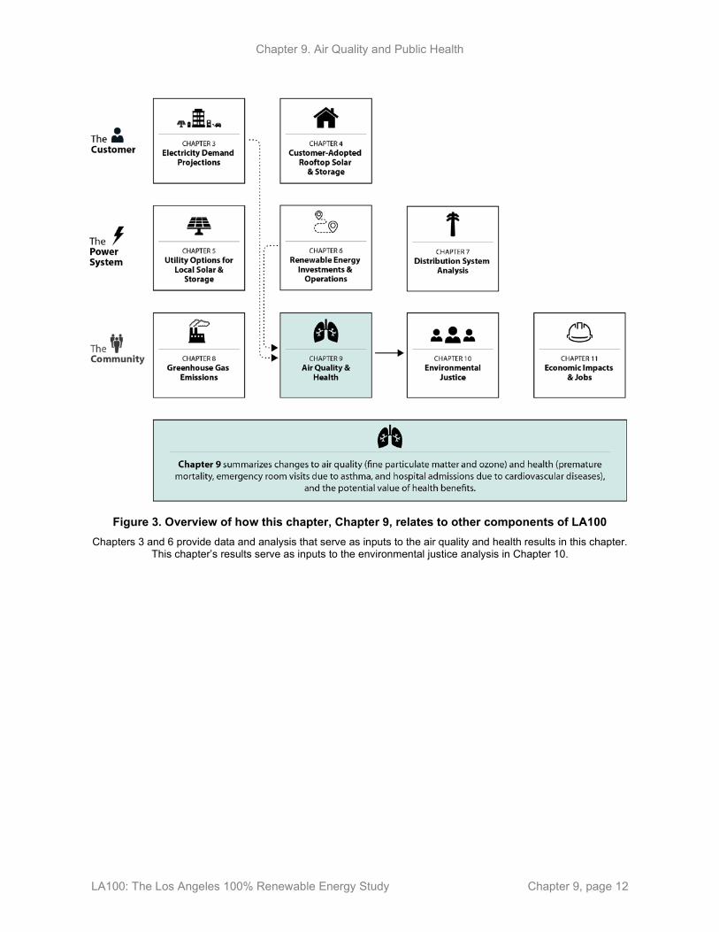
Figure 3. Overview of how this chapter, Chapter 9, relates to other components of LA100
Chapters 3 and 6 provide data and analysis that serve as inputs to the air quality and health results in this chapter. This chapter’s results serve as inputs to the environmental justice analysis in Chapter 10.

Chapter 9. Air Quality and Public Health
LA100: The Los Angeles 100% Renewable Energy Study Chapter 9, page 13
2 Methodology and Data 2.1 Air Quality Modeling
2.1.1 General Description of Air Quality Modeling Air quality modeling involves simulating the physics and chemistry of the atmosphere in order to quantify how emitted air pollutants disperse and react in the atmosphere. Air quality models take emissions as inputs and simulate both meteorology, which determines how the emissions are dispersed, and atmospheric chemistry, which determines how the emissions are chemically transformed. The emissions inputs (known as “emissions inventories”) specify where, when, and how much of each pollutant is emitted. They report emissions for pollutants relevant to the formation of O3 and PM2.5, such as volatile organic compounds (VOC), oxides of nitrogen (NOx), ammonia (NH3), primary PM, and sulfur oxides (SOx). Pollutant transport is determined using simulated meteorological variables such as temperature, wind speed, and planetary (atmospheric) boundary layer height, which are calculated based on numerically solving laws of physics. Transformation of pollutants via atmospheric chemistry is simulated by numerically solving equations that describe known chemical reactions for both gas- and particle-phase species. These chemical reactions can form “secondary” pollutants of interest (e.g., O3) and also transform emitted gas-phase species to particle phase pollutants.
2.1.2 Model Selection and Justification In this study we use a state-of-the-science, regional meteorology and chemistry model, the Weather Research and Forecasting model coupled with Chemistry Version 3.74 (WRF-Chem v3.7). WRF-Chem was developed at the National Center for Atmospheric Research (NCAR), which is operated by the University Corporation for Atmospheric Research (UCAR). It is an open-source, community model commonly used by researchers and regulators (Chen et al., 2013; Yahya et al., 2015; Li et al., 2019; Zhang et al., 2019; Wang et al., 2020). WRF-Chem has been widely used for air quality studies targeted at Southern California since its release in 2005 (Grell et al., 2005), including several by the investigators of this project (Chen et al., 2013; Li et al., 2019; Zhang et al., 2019; Wang et al., 2020). Past studies using this model include evaluating how urbanization has affected historical air quality (Chen et al., 2013; Li et al., 2019), and investigating how future changes in emissions or land use could alter air quality (Zhang et al., 2019; Wang et al., 2020).
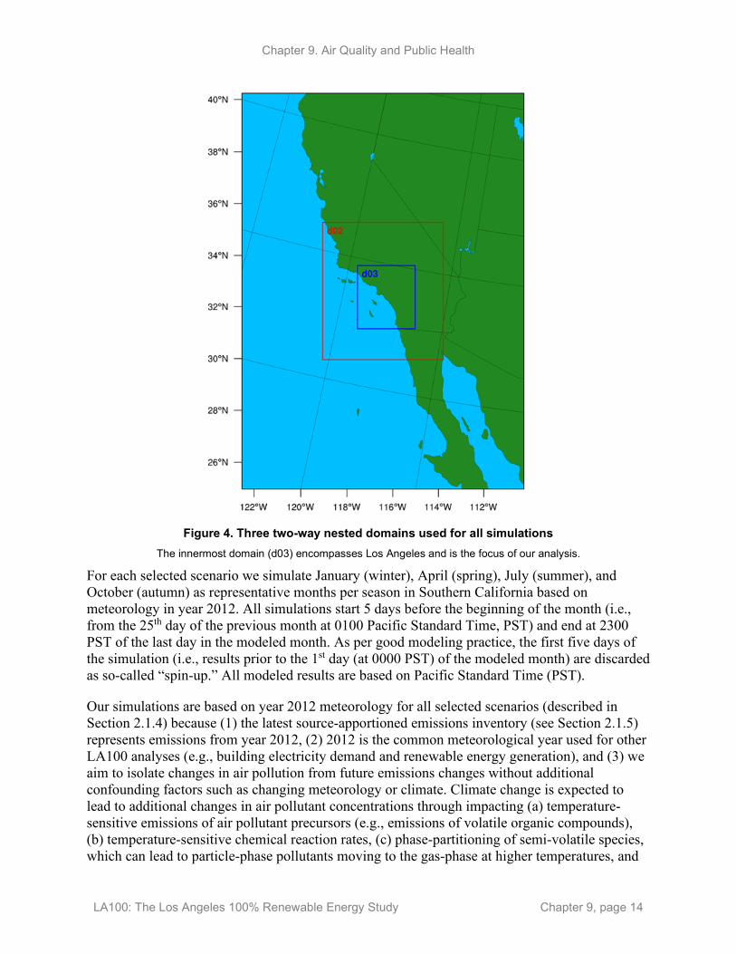
2.1.3 Model Domain and Time Period All simulations are performed using three two-way nested domains at horizontal resolutions of 18 km, 6 km, and 2 km, respectively, as shown in Figure 4. The outer two domains encompass most of California and provide boundary conditions to the innermost domain, which covers Southern California. Los Angeles is located in the innermost domain (d03) and is the focus of our model analysis. Each domain uses 29 layers in the vertical from the ground to 100 hPa, although only the lowest atmospheric layer is used for analysis of pollutant concentrations.
4 Available for download at “Weather Research and Forecasting Model Coupled to Chemistry (WRF-Chem),” NOAA, https://ruc.noaa.gov/wrf/wrf-chem/.
Chapter 9. Air Quality and Public Health
LA100: The Los Angeles 100% Renewable Energy Study Chapter 9, page 14
Figure 4. Three two-way nested domains used for all simulations
The innermost domain (d03) encompasses Los Angeles and is the focus of our analysis.
For each selected scenario we simulate January (winter), April (spring), July (summer), and October (autumn) as representative months per season in Southern California based on meteorology in year 2012. All simulations start 5 days before the beginning of the month (i.e., from the 25th day of the previous month at 0100 Pacific Standard Time, PST) and end at 2300 PST of the last day in the modeled month. As per good modeling practice, the first five days of the simulation (i.e., results prior to the 1st day (at 0000 PST) of the modeled month) are discarded as so-called “spin-up.” All modeled results are based on Pacific Standard Time (PST).
Our simulations are based on year 2012 meteorology for all selected scenarios (described in Section 2.1.4) because (1) the latest source-apportioned emissions inventory (see Section 2.1.5) represents emissions from year 2012, (2) 2012 is the common meteorological year used for other LA100 analyses (e.g., building electricity demand and renewable energy generation), and (3) we aim to isolate changes in air pollution from future emissions changes without additional confounding factors such as changing meteorology or climate. Climate change is expected to lead to additional changes in air pollutant concentrations through impacting (a) temperature-sensitive emissions of air pollutant precursors (e.g., emissions of volatile organic compounds), (b) temperature-sensitive chemical reaction rates, (c) phase-partitioning of semi-volatile species, which can lead to particle-phase pollutants moving to the gas-phase at higher temperatures, and

Chapter 9. Air Quality and Public Health
LA100: The Los Angeles 100% Renewable Energy Study Chapter 9, page 15
(d) future changes in meteorological variables that impact removal of pollutants from Los Angeles (e.g., winds and precipitation). There remains uncertainty on the net effect of these various pathways on air pollution. Future analysis could consider simultaneous impacts from climate change on air quality and subsequent health impacts.
Model performance was evaluated by comparing simulated daily 8-hour maximum O3 and daily average PM2.5 concentrations from the baseline scenario (see Section 2.1.4) to historical observations. A detailed description of observational data sources and model performance results can be found in Appendix B. In summary, these model evaluation tests helped to diagnose some improvements we implemented in the model for better simulation of chemistry in and around LA; the final, revised model configuration passed best-practice quality criteria used by the air quality modeling community (reported in Appendix B).
2.1.4 Scenarios for Analysis We assess air quality co-benefits of pathways to achieve 100% renewable energy by first considering 2012 as a baseline, and then comparing among selected LA100 scenarios. The LA100 scenarios of focus (SB100 and Early & No Biofuels, both Moderate and High Load Electrification) represent different power sector eligibility criteria and electrical load levels, which ultimately affect emissions from power plants, transportation, buildings, and the Ports of Los Angeles and Long Beach. Our air quality assessment focuses on the final LA100 modeled year, 2045. Note that we chose 2045 for our analysis (even though Early & No Biofuels meets the 100% renewable energy goal 10 years earlier) in order to achieve consistency between the selected LA100 scenarios, and with electricity demand projections in Chapter 3 and bulk power system analyses in Chapter 6.
LA100 scenarios were designed to provide contrast in development of the LADWP grid assets toward a 100% renewable energy future. Many aspects of power supply and electricity demand can have little or no impact on air pollutant emissions. Thus, we select the LA100 scenarios (SB100 and Early & No Biofuels) for air quality analysis with the aim of identifying which would demonstrate the greatest contrast in air pollutant concentrations balanced with a general desire for consistency with other impacts analyses in LA100.
By analyzing differences in the chosen LA100 scenarios we can isolate the effects of two key aspects (i.e., electrification levels and power plant fuel type) contributing to air pollution relevant to this study. The SB100 scenario allows the use of renewable energy credits to offset a portion of power generation provided by fossil fuel combustion. Early & No Biofuels represents a scenario that achieves compliance with a more stringent 100% renewable energy definition among LADWP-owned power generation utilities (e.g., no renewable energy certificates are allowed, nor biofuel combustion for power generation) 10 years earlier than for SB100 (i.e., in 2035). Each of these scenarios is evaluated at two levels of load electrification (Moderate and High) from sources within the transportation, industrial, and building sectors.
Table 5 summarizes the various assumptions for energy supply and demand used for the selected LA100 scenarios: Baseline (2012), SB100 – Moderate Load Electrification (referred to hereafter as SB100 – Moderate), SB100 – High Load Electrification (SB100 – High), Early & No Biofuels – Moderate Load Electrification (Early & No Biofuels – Moderate) and Early & No Biofuels – Moderate Load Electrification (Early & No Biofuels – High). The effects of excluding natural

Chapter 9. Air Quality and Public Health
LA100: The Los Angeles 100% Renewable Energy Study Chapter 9, page 16
gas power plants can be isolated by comparing Early & No Biofuels – Moderate with SB100 – Moderate, or Early & No Biofuels – High with SB100 – High. The SB100 – Moderate and Early & No Biofuels – Moderate scenarios assume moderate electrification levels for the LA100-influenced emission sources (see Table 6, Table 7, and Table 8), while the SB100 – High and Early & No Biofuels – High scenarios assume high electrification levels. The effects of varying electrification levels in end-use sectors, including transportation (specifically, light-duty vehicles [LDVs]), residential and commercial buildings, and the Ports (specifically, ocean-going vessels [OGVs]) can be assessed by comparing SB100 – High with SB100 – Moderate, and Early & No Biofuels – High with Early & No Biofuels – Moderate. In addition, the combined effects of electrification and shutting down natural gas power plants at LADWP-owned sites can be investigated by comparing Early & No Biofuels – High and SB100 – Moderate. Thus, SB100 – Moderate is used as a reference case for the selected future scenarios as it is the closest representation of the legal mandates that currently exist, allows some natural gas generation, and assumes lower electrification levels. The definitions of Moderate and High electrification levels for LA100 emission sources are described in detail in Chapter 3. A summary of those definitions is shown in Table 6, Table 7, and Table 8.
Table 5. Scenario Names and Key Assumptions Used for Analyzing Air Pollutant Emissions and Air Quality Co-Benefits
Scenario Name (and Abbreviation)
LADWP-Owned Power Plants Can Burn Natural Gas?a
LADWP-Owned Power Plants Can Burn Hydrogen?b
Electrification Level for LDVs and Buses, Commercial and Residential Buildings, and the Ports
1. Baseline (2012) N/A N/A N/A
2. SB100 – Moderate (SB100 – M)
Yes Yes Moderate
3. SB100 – High (SB100 – H)
Yes Yes High
4. Early & No Biofuels – Moderate (Early & No Biofuels – M)
No Yes Moderate
5. Early & No Biofuels – High (Early & No Biofuels – H)
No Yes High
a Burning natural gas would necessitate the utility to purchase renewable energy certificates to meet the requirements of SB100. b LADWP-owned power plants are assumed to burn 100% hydrogen by 2045 to the extent they are utilized. Note that while biofuels are allowed in years prior to 2045 in the SB100 scenario, they are not allowed starting in 2045.

Chapter 9. Air Quality and Public Health
LA100: The Los Angeles 100% Renewable Energy Study Chapter 9, page 17
Table 6. Fraction of Light-Duty Vehicles and Buses That Are Assumed to Be Electric Powered in 2045 for Moderate and High Electrification Levels
Emission Source Moderate Electrification High Electrification
Light-duty vehicles 30% of stock is plug-in electric vehiclesa (PEV) 80% of stock is PEV
School and urban buses 100% 100%
a PEVs consist of 50% plug-in hybrid vehicles and 50% battery electric vehicles
Table 7. Fraction of Buildings/Households by End Use That Are Assumed to Be Electric Powered in 2045 for Moderate and High Electrification
Emission Source End Use Moderate Electrification High Electrification
Commercial building Water heating 72% 100%
Space heating 81% 96%
Residential building
Water heating 50% 100%
Space heating 49% 91%
Clothes drying 93% 100%
Cooking 53% 100%
Table 8. Fraction of Port Sources That Are Assumed to Be Electric Powered in 2045 for both Moderate and High Electrification in the Air Quality Analysisa
Emission Source Moderate Electrification
High Electrification
Ocean-Going Vessels (OGVs, shore power at berth) 80% 90%
Cargo Handling Equipment (CHE) 100% 100%
Heavy-Duty Vehicles (HDVs) 100% 100%
a The assumptions of electrification levels for emissions from cargo handling equipment and heavy-duty vehicles at the Ports are based on the most up-to-date 2017 Clean Air Action Plan (https://cleanairactionplan.org/), and they differ from what is used in the rest of the LA100 study. In addition, we assume the moderate and high electrification are applicable to both the Port of Los Angeles and the Port of Long Beach instead of just the Port of Los Angeles. These changes at the Ports are expected to have minimal effect on power generation projected overall in 2045, and thus the discrepancy between modeling assumptions among these chapters does not make the results of air quality modeling inconsistent with the power sector modeling performed in this study in a significant way.
2.1.5 Emission Inventory Development
2.1.5.1 Baseline Emission Inventory Gridded hourly emissions for the Baseline (2012) scenario for the innermost domain are constructed based on gridded source-specific raw emissions obtained from the South Coast Air Quality Management District (SCAQMD). The SCAQMD emissions data set for year 2012 is the most recent emissions inventory available from the SCAQMD, as described in their 2016 Air Quality Management Plan Appendix III: Base and Future Year Emission Inventory (South Coast

Chapter 9. Air Quality and Public Health
LA100: The Los Angeles 100% Renewable Energy Study Chapter 9, page 18
Air Quality Management District, 2017). It is a source-apportioned emissions inventory, which is crucial for creating emissions projections by end use (explained in more detail in the following sections). Annual-averaged daily emissions are provided for carbon monoxide (CO), NOx, SOx, total organic gases (TOG), Total Suspended Particles (TSP), and ammonia (NH3). Point sources (e.g., emissions from electricity generation) are provided by Source Classification Code (SCC), and area sources (e.g., emissions from commercial and residential buildings) and mobile sources are by Emission Inventory Code (EIC). Raw emissions are processed to gridded hourly emissions from all sources using associated temporal profiles per emission source, and to chemical species in the SAPRC chemical mechanism using associated speciation profiles per source (Carter, 2003). More detail on the speciation of emission inventory can be found in Appendix B.
Anthropogenic emissions for the two outer domains in all scenarios are adopted from the 2012 emissions inventory from the California Air Resource Board (CARB) for areas within California (California Air Resources Board, 2017), and from the 2011 National Emission Inventory (NEI) for regions outside California (U.S. EPA, 2014). For these two outer domains, we use the same emissions inventories for the 2012 Baseline and future scenarios to avoid adding additional sources of variability; emissions from these outer domains are expected to have small impact on air quality in Los Angeles. Biogenic emissions are generated by the Model of Emissions of Gases and Aerosols from Nature (MEGAN) coupled to WRF-Chem using model predicted meteorological conditions (Guenther et al., 2006). In addition, emissions from wildfire are not included in our simulations.
2.1.5.2 Emission Inventory Development for Selected LA100 Scenarios in 2045 For emissions sources within Los Angeles that are influenced by LA100, we project emissions for future scenarios based on four factors:
1. Gridded, source-apportioned, raw emissions (either from the 2012 Baseline, or 2031 projections from SCAQMD if factors for scaling activity from 2031 to 2045 are available) (See Appendix B for more explanation)
2. Activity projections (either from LA100 energy model input assumptions and outputs described in Chapter 6 or, when not available, from regulatory agencies)
3. Emission factor projections (from regulatory agencies and past studies), and 4. Electrification projections (from LA100 electricity demand projections presented in
Chapter 3). For emissions sources not influenced by LA100 (e.g., heavy-duty trucks outside the Ports), and all emissions sources outside Los Angeles, we adopt emissions projections from SCAQMD for the year 2031. Examples of emission control strategies that are accounted in the SCAQMD projected inventory include for heavy-duty vehicles the On-Road Heavy-Duty Diesel Vehicles Regulation implemented by CARB, and the Accelerated Retirement of Older On-Road Heavy-Duty Vehicles implemented by CARB and SCAQMD (SCAQMD, 2017). Details on control strategies for all sources considered in SCAQMD's emission projection can be found in Chapter 4, Appendix IV and Appendix VI of the “Final 2016 Air Quality Management Plan” (SCAQMD, 2017). Given that SCAQMD has not developed projections for pollutant emissions past 2031, we assume these emissions stay constant from 2031 to 2045.

Chapter 9. Air Quality and Public Health
LA100: The Los Angeles 100% Renewable Energy Study Chapter 9, page 19
Emissions inventory development for each LA100 source sector is described in the following subsections. In short, we project absolute emissions based on fuel consumption and emission factors for the power sector, and scale baseline emissions (from year 2012 or 2031) using activity, emissions factors, and electrification levels for emissions from the transportation sector, residential and commercial buildings, and the Ports. While the scaling method aligns with our emissions data and is the method applied in past relevant studies (Zapata et al., 2018a; Wang et al., 2020), we calculate emissions from LADWP-owned power plants directly from fuel consumption and emission factors for the following two reasons. First, some LADWP-owned power plant units have been modified since 2012 and thus these changes to emissions have not been considered in the SCAQMD emission inventories. Second, there is no consistent data source for generating scaling factors for fuel consumption of power plants.
2.1.5.2.1 Emission Inventory Development for Electricity Generation Selected future scenarios differ in their assumptions on fuel eligibility for LADWP-owned power plants (see Table 5). Natural gas combustion turbine and combined cycle power plants are allowed in the SB100 scenario, while hydrogen combustion turbines are allowed in both SB100 and Early & No Biofuels. To project power plant activity in 2045, we use hourly fuel consumption projected by the PLEXOS Electricity Market Simulation model described in Chapter 6. Emission factors for power plants in 2045 are based on data from current power plants along with regulatory limits (more details are below). Emissions in 2045 from power plants owned by utilities other than LADWP follow the SCAQMD projection to year 2031, and assume they are constant from 2031 to 2045.
Emissions generated from LADWP-owned power plants in 2045 for a given scenario are quantified as:
𝐸𝐸𝐸𝐸𝐸𝐸𝐸𝐸𝐸𝐸_𝑃𝑃𝑃𝑃𝑃𝑃𝑃𝑃𝑃𝑃𝑝𝑝,𝑝𝑝𝑝𝑝𝑝𝑝𝑝𝑝𝑝𝑝,2045 = 𝐹𝐹𝐹𝐹_𝑃𝑃𝑃𝑃𝑃𝑃𝑃𝑃𝑃𝑃𝑝𝑝𝑝𝑝𝑝𝑝𝑝𝑝𝑝𝑝,2045 × 𝐸𝐸𝐹𝐹_𝑃𝑃𝑃𝑃𝑃𝑃𝑃𝑃𝑃𝑃𝑝𝑝,𝑝𝑝𝑝𝑝𝑝𝑝𝑝𝑝𝑝𝑝,2045
(Eq. 2.1.5.2.1-1)
where 𝐸𝐸𝐸𝐸𝐸𝐸𝐸𝐸𝐸𝐸_𝑃𝑃𝑃𝑃𝑃𝑃𝑃𝑃𝑃𝑃𝑝𝑝,𝑝𝑝𝑝𝑝𝑝𝑝𝑝𝑝𝑝𝑝,2045 (kg/hour) represents emissions of pollutant p from a specific power plant power at hourly resolution, 𝐹𝐹𝐹𝐹_𝑃𝑃𝑃𝑃𝑃𝑃𝑃𝑃𝑃𝑃𝑝𝑝𝑝𝑝𝑝𝑝𝑝𝑝𝑝𝑝,2045 (one million British Thermal Units (MMBTU)/hour) is fuel consumption (natural gas or hydrogen, depending on scenario) of the power plant at hourly resolution from the PLEXOS model, and 𝐸𝐸𝐹𝐹_𝑃𝑃𝑃𝑃𝑃𝑃𝑃𝑃𝑃𝑃𝑝𝑝,𝑝𝑝𝑝𝑝𝑝𝑝𝑝𝑝𝑝𝑝,2045 ( kg/MMBTU) is the emission factor for pollutant p (i.e., CO, NOx, SOx, TOG, TSP and NH3) from the power plant in year 2045. Values for each term vary by scenario.
Emission factors for natural gas power plants in SB100 are based on calculated values from the latest available (year 2019) LADWP emissions reporting system (LADWP, 2019). Thus, for SB100 we assume that current power plants will maintain constant emission factors until 2045, except for NOx and NH3 emissions. For these two pollutants, if the calculated emission factor exceeds SCAQMD current regulation limits RULE 1135 (South Coast Air Quality Management District, 2018), we modify the emission factor according to the applicable regulatory limits assuming that the emissions will be brought back into compliance. For hydrogen-fueled combustion turbines, we assume that emission factors for SOx, TSP, TOG and CO are zero since hydrogen fuel does not contain carbonaceous or sulfuric species. For NOx and NH3 emission factors from H2 combustion, we follow the aforementioned current regulation limit for natural

Chapter 9. Air Quality and Public Health
LA100: The Los Angeles 100% Renewable Energy Study Chapter 9, page 20
gas combustion turbines as an upper bound based on the assumption that future hydrogen power plants will meet the emissions regulations of current power plants. A table including assumed emission factors for every LADWP-owned power plant is in Appendix B.
2.1.5.2.2 Emission Inventory Development for the Transportation Sector For the transportation sector, we project emissions to 2045 for sources included in LA100 load modeling: light-duty vehicles (including passenger cars and light-duty trucks) and buses (i.e., school bus and urban bus) in Los Angeles. The projected emissions are based on (a) source-specific emissions projections to 2031 from SCAQMD (South Coast Air Quality Management District, 2017), (b) assumptions on vehicle activity (i.e., vehicle populations and vehicle miles traveled) from the California Air Resources Board (CARB) EMission FACtor (EMFAC) model (California Air Resources Board, 2014), (c) emission factor projections also from the CARB EMFAC model, and (d) assumptions on electrification level changes from electricity demand projections described in Chapter 3. Emissions in 2045 for vehicle types that are not influenced by LA100 (i.e., motorcycles, medium-duty vehicles and heavy-duty vehicles, and bus types other than school and urban buses), follow the SCAQMD projection to year 2031, and assume they are constant from 2031 to 2045.
Emissions per grid cell for pollutant p from LDVs and buses in Los Angeles for year 2045 (𝐸𝐸𝐸𝐸𝐸𝐸𝐸𝐸𝐸𝐸_𝑉𝑉𝑃𝑃ℎ𝑝𝑝,2045, in unit of kg/day) are calculated as the sum of emissions from non-electric vehicles (𝐸𝐸𝐸𝐸𝐸𝐸𝐸𝐸𝐸𝐸_𝑁𝑁𝑃𝑃𝑁𝑁𝐸𝐸𝑙𝑙𝑃𝑃𝑙𝑙_𝑉𝑉𝑃𝑃ℎ𝑝𝑝,𝑣𝑣,𝑓𝑓,𝑝𝑝𝑝𝑝,2045) and electric vehicles (𝐸𝐸𝐸𝐸𝐸𝐸𝐸𝐸𝐸𝐸_𝐸𝐸𝑙𝑙𝑃𝑃𝑙𝑙_𝑉𝑉𝑃𝑃ℎ𝑝𝑝,𝑣𝑣,𝑝𝑝𝑒𝑒𝑝𝑝𝑝𝑝,𝑝𝑝𝑝𝑝,2045) as shown by Eq. 2.1.5.2.2-1.
𝐸𝐸𝐸𝐸𝐸𝐸𝐸𝐸𝐸𝐸_𝑉𝑉𝑃𝑃ℎ𝑝𝑝,2045 = ∑ 𝐸𝐸𝐸𝐸𝐸𝐸𝐸𝐸𝐸𝐸_𝑁𝑁𝑃𝑃𝑁𝑁𝐸𝐸𝑙𝑙𝑃𝑃𝑙𝑙_𝑉𝑉𝑃𝑃ℎ𝑣𝑣,𝑓𝑓,𝑝𝑝𝑝𝑝 𝑝𝑝,𝑣𝑣,𝑓𝑓,𝑝𝑝𝑝𝑝,2045+
∑ 𝐸𝐸𝐸𝐸𝐸𝐸𝐸𝐸𝐸𝐸_𝐸𝐸𝑙𝑙𝑃𝑃𝑙𝑙_𝑉𝑉𝑃𝑃ℎ𝑝𝑝,𝑣𝑣,𝑝𝑝𝑒𝑒𝑝𝑝𝑝𝑝,𝑝𝑝𝑝𝑝,2045𝑣𝑣,𝑝𝑝𝑝𝑝
(Eq. 2.1.5.2.2-1)
where v stands for a vehicle type, f is the fuel type (i.e., gasoline or diesel) used by the non-electric vehicle, and pc represents the process that emits pollutants (i.e., diurnal evaporative emissions, hot soak evaporative emissions, running evaporative emissions, rest evaporative emissions, start exhaust emissions, running exhaust emissions, idling exhaust emissions, tire wear emissions and break wear emissions).
Gridded emissions for pollutant p in year 2045 from a non-electric vehicle (𝐸𝐸𝐸𝐸𝐸𝐸𝐸𝐸𝐸𝐸_𝑁𝑁𝑃𝑃𝑁𝑁𝐸𝐸𝑙𝑙𝑃𝑃𝑙𝑙_𝑉𝑉𝑃𝑃ℎ𝑝𝑝,𝑣𝑣,𝑓𝑓,𝑝𝑝𝑝𝑝,2045) are projected by applying a scaling factor to the SCAQMD projections for year 2031. The scaling factor is calculated as the product of four terms as shown in Eq. 2.1.5.2.2-2: (a) the ratio of emissions from a specific vehicle type to the total emissions from all vehicle types in 2031 (from EMFAC), (b) the ratio of vehicle activity projected for a specific vehicle type between year 2045 to 2031 (from EMFAC), (c) the ratio of emission factors for an emitting process of a specific vehicle type between 2045 to 2031 (from EMFAC), and (d) one minus the fraction of vehicles registered in Los Angeles that are electric vehicles. More specifically, 𝐸𝐸𝐸𝐸𝐸𝐸𝐸𝐸𝐸𝐸_𝑁𝑁𝑃𝑃𝑁𝑁𝐸𝐸𝑙𝑙𝑃𝑃𝑙𝑙_𝑉𝑉𝑃𝑃ℎ𝑝𝑝,𝑣𝑣,𝑓𝑓,𝑝𝑝𝑝𝑝,2045 is calculated as

Chapter 9. Air Quality and Public Health
LA100: The Los Angeles 100% Renewable Energy Study Chapter 9, page 21
𝐸𝐸𝐸𝐸𝐸𝐸𝐸𝐸𝐸𝐸_𝑁𝑁𝑃𝑃𝑁𝑁𝐸𝐸𝑙𝑙𝑃𝑃𝑙𝑙_𝑉𝑉𝑃𝑃ℎ𝑝𝑝,𝑣𝑣,𝑓𝑓,𝑝𝑝𝑝𝑝,2045 = 𝐸𝐸𝐸𝐸𝐸𝐸𝐸𝐸𝐸𝐸_𝑉𝑉𝑃𝑃ℎ𝑝𝑝,2031 × 𝐸𝐸𝐸𝐸𝐸𝐸𝐸𝐸𝐸𝐸_𝑉𝑉𝑝𝑝ℎ𝑝𝑝,𝑣𝑣,𝑓𝑓,𝑝𝑝𝑝𝑝,2031
∑ 𝐸𝐸𝐸𝐸𝐸𝐸𝐸𝐸𝐸𝐸_𝑉𝑉𝑝𝑝ℎ𝑝𝑝,𝑣𝑣,𝑓𝑓,𝑝𝑝𝑝𝑝,2031𝑣𝑣,𝑓𝑓,𝑝𝑝𝑝𝑝×
𝐴𝐴_𝑉𝑉𝑝𝑝ℎ𝑣𝑣,𝑓𝑓,𝑝𝑝𝑝𝑝,2045
𝐴𝐴_𝑉𝑉𝑝𝑝ℎ𝑣𝑣,𝑓𝑓,𝑝𝑝𝑝𝑝,2031× 𝐸𝐸𝐸𝐸_𝑉𝑉𝑝𝑝ℎ𝑝𝑝,𝑣𝑣,𝑓𝑓,𝑝𝑝𝑝𝑝,2045
𝐸𝐸𝐸𝐸_𝑉𝑉𝑝𝑝ℎ𝑝𝑝,𝑣𝑣,𝑓𝑓,𝑝𝑝𝑝𝑝,2031× (1 − 𝐸𝐸𝑙𝑙𝑃𝑃𝑙𝑙_𝑉𝑉𝑃𝑃ℎ𝑣𝑣,2045)
(Eq. 2.1.5.2.2-2)
where 𝐸𝐸𝐸𝐸𝐸𝐸𝐸𝐸𝐸𝐸_𝑉𝑉𝑃𝑃ℎ𝑝𝑝,2031 (kg/day) is the gridded emission for pollutant p from all vehicle types in year 2031 provided by SCAQMD, 𝐸𝐸𝐸𝐸𝐸𝐸𝐸𝐸𝐸𝐸_𝑉𝑉𝑝𝑝ℎ𝑝𝑝,𝑣𝑣,𝑓𝑓,𝑝𝑝𝑝𝑝,2031
∑ 𝐸𝐸𝐸𝐸𝐸𝐸𝐸𝐸𝐸𝐸_𝑉𝑉𝑝𝑝ℎ𝑝𝑝,𝑣𝑣,𝑓𝑓,𝑝𝑝𝑝𝑝,2031𝑣𝑣,𝑓𝑓,𝑝𝑝𝑝𝑝 is the ratio of emissions from vehicle
type v using fuel type f to all transportation emissions (unitless) based on EMFAC, 𝐴𝐴_𝑉𝑉𝑃𝑃ℎ𝑣𝑣,𝑓𝑓,2031 and 𝐴𝐴_𝑉𝑉𝑃𝑃ℎ𝑣𝑣,𝑓𝑓,2045 are activity projections per vehicle and fuel type in year 2031 and 2045 respectively (units for A_Veh are number of vehicles for vehicle population and miles/day for vehicle miles traveled, VMT, 𝐴𝐴_𝑉𝑉𝑝𝑝ℎ𝑣𝑣,𝑓𝑓,𝑝𝑝𝑝𝑝,2045
𝐴𝐴_𝑉𝑉𝑝𝑝ℎ𝑣𝑣,𝑓𝑓,𝑝𝑝𝑝𝑝,2031 is unitless), 𝐸𝐸𝐹𝐹_𝑉𝑉𝑃𝑃ℎ𝑝𝑝,𝑣𝑣,𝑓𝑓,𝑝𝑝𝑝𝑝,2031 and
𝐸𝐸𝐹𝐹_𝑉𝑉𝑃𝑃ℎ𝑝𝑝,𝑣𝑣,𝑓𝑓,𝑝𝑝𝑝𝑝,2045 are emission factors per vehicle, fuel type and emitting process in year 2031 and 2045 respectively (units for EF_Veh are kg/vehicle/day for vehicle-population-based calculation and kg/mile for VMT-based calculation, 𝐸𝐸𝐸𝐸_𝑉𝑉𝑝𝑝ℎ𝑝𝑝,𝑣𝑣,𝑓𝑓,𝑝𝑝𝑝𝑝,2045
𝐸𝐸𝐸𝐸_𝑉𝑉𝑝𝑝ℎ𝑝𝑝,𝑣𝑣,𝑓𝑓,𝑝𝑝𝑝𝑝,2031 is unitless), and
𝐸𝐸𝑙𝑙𝑃𝑃𝑙𝑙_𝑉𝑉𝑃𝑃ℎ𝑣𝑣,2045 is the fraction of vehicles per vehicle type that are electric in year 2045, obtained from the transportation model Electric Vehicle Infrastructure Projection Tool (EVI-Pro) described in Chapter 3 (Wood, Rames and Muratori, 2018). Values for 𝐸𝐸𝐸𝐸𝐸𝐸𝐸𝐸𝐸𝐸_𝑉𝑉𝑃𝑃ℎ(𝐸𝐸𝐸𝐸𝐹𝐹𝐴𝐴𝐹𝐹)𝑝𝑝,𝑣𝑣,𝑓𝑓,2031, 𝐸𝐸𝐸𝐸𝐸𝐸𝐸𝐸𝐸𝐸_𝑉𝑉𝑃𝑃ℎ(𝐸𝐸𝐸𝐸𝐹𝐹𝐴𝐴𝐹𝐹)𝑝𝑝,2031, 𝐴𝐴𝐹𝐹_𝑉𝑉𝑃𝑃ℎ𝑣𝑣,𝑓𝑓,2031, 𝐴𝐴𝐹𝐹_𝑉𝑉𝑃𝑃ℎ𝑣𝑣,𝑓𝑓,2045, 𝐸𝐸𝐹𝐹_𝑉𝑉𝑃𝑃ℎ𝑝𝑝,𝑣𝑣,𝑓𝑓,𝑝𝑝𝑝𝑝,2031 and 𝐸𝐸𝐹𝐹_𝑉𝑉𝑃𝑃ℎ𝑝𝑝,𝑣𝑣,𝑓𝑓,𝑝𝑝𝑝𝑝,2045 are determined using annual averaged data from the EMFAC2014 model applied to Los Angeles County (except the Mojave Desert region). We chose EMFAC2014 (rather than newer EMFAC versions) because SCAQMD used this version for developing the inventories used in our baseline. The electrification level 𝐸𝐸𝑙𝑙𝑃𝑃𝑙𝑙_𝑉𝑉𝑃𝑃ℎ𝑣𝑣,2045 for all vehicle types within the LDV category (i.e., passenger cars and light-duty trucks) have the same value for each scenario. Values for these variables can be found in Appendix B.
Emissions from electric LDVs and buses in year 2045 need to be considered since they have non-zero emission factors for PM from brake wear and tire wear. Note that EMFAC2014 suggests that electric LDVs have nonzero evaporative TOG emissions, but we ignore these since they are negligible in magnitude. We assume that tire wear PM emission factors per vehicle category are identical for electric versus non-electric vehicles in 2045. Brake wear emission factors per vehicle category are reduced by 59% for electric vehicles (relative to non-electric vehicles) due to regenerative braking (Timmers and Achten, 2018). Eq. 2.1.5.2.2-3 is used for quantifying tire and brake wear emissions from electric LDVs and buses.
𝐸𝐸𝐸𝐸𝐸𝐸𝐸𝐸𝐸𝐸_𝐸𝐸𝑙𝑙𝑃𝑃𝑙𝑙_𝑉𝑉𝑃𝑃ℎ𝑝𝑝,𝑣𝑣,𝑝𝑝𝑒𝑒𝑝𝑝𝑝𝑝,𝑝𝑝𝑝𝑝,2045
= 𝐸𝐸𝐸𝐸𝐸𝐸𝐸𝐸𝐸𝐸_𝑉𝑉𝑃𝑃ℎ𝑝𝑝,2031 ×𝐸𝐸𝐸𝐸𝐸𝐸𝐸𝐸𝐸𝐸_𝑉𝑉𝑃𝑃ℎ𝑝𝑝,𝑣𝑣,𝑓𝑓,2031
𝐸𝐸𝐸𝐸𝐸𝐸𝐸𝐸𝐸𝐸_𝑉𝑉𝑃𝑃ℎ𝑝𝑝,2031×𝐴𝐴_𝑉𝑉𝑃𝑃ℎ𝑣𝑣,𝑓𝑓,2045
𝐴𝐴_𝑉𝑉𝑃𝑃ℎ𝑣𝑣,𝑓𝑓,2031
×𝐸𝐸𝐹𝐹_𝑉𝑉𝑃𝑃ℎ𝑝𝑝,𝑣𝑣,𝑓𝑓,𝑝𝑝𝑝𝑝,2045
𝐸𝐸𝐹𝐹_𝑉𝑉𝑃𝑃ℎ𝑝𝑝,𝑣𝑣,𝑓𝑓,𝑝𝑝𝑝𝑝,2031×𝐸𝐸𝐹𝐹_𝑉𝑉𝑃𝑃ℎ𝑝𝑝,𝑣𝑣,𝑝𝑝𝑒𝑒𝑝𝑝𝑝𝑝,𝑝𝑝𝑝𝑝,2045
𝐸𝐸𝐹𝐹_𝑉𝑉𝑃𝑃ℎ𝑝𝑝,𝑣𝑣,𝑓𝑓,𝑝𝑝𝑝𝑝,2045× 𝐸𝐸𝑙𝑙𝑃𝑃𝑙𝑙_𝑉𝑉𝑃𝑃ℎ𝑣𝑣,2045
(Eq. 2.1.5.2.2-3)

Chapter 9. Air Quality and Public Health
LA100: The Los Angeles 100% Renewable Energy Study Chapter 9, page 22
where the new term 𝐸𝐸𝐸𝐸_𝑉𝑉𝑝𝑝ℎ𝑝𝑝,𝑣𝑣,𝑒𝑒𝑒𝑒𝑒𝑒𝑝𝑝,𝑝𝑝𝑝𝑝,2045
𝐸𝐸𝐸𝐸_𝑉𝑉𝑝𝑝ℎ𝑝𝑝,𝑣𝑣,𝑓𝑓,𝑝𝑝𝑝𝑝,2045 represents the ratio of emission factors for electric vehicles
to non-electric vehicles.
2.1.5.2.3 Emission Inventory Development for Commercial and Residential Buildings Emissions projections for commercial and residential buildings account for reductions in natural gas consumption from various end uses as electrification is increased. Natural gas fuel use is projected using ResStock™ and ComStock™ within the demand-side grid model, dsgrid, as described in Chapter 3 (Hale et al., 2018). The models use year 2020 as an initial state and projects natural gas consumption to year 2045 in 5-years increments for Los Angeles under moderate and high electrification level assumptions. We project emissions from commercial and residential buildings to 2045 in two steps. First, we project emissions from these sectors in Los Angeles from year 2012 to 2020 using gridded source-specific 2012 emissions by applying scaling factors representing activity growth and emission factor changes between 2012 and 2020, both taken from SCAQMD (South Coast Air Quality Management District, 2017). We do this first step to match the 2020 base year of the dsgrid simulations. Secondly, we project emissions from year 2020 to 2045 based on scaling factors that represent changes in activity (i.e., natural gas consumption from dsgrid) and emission factors. Scaling factors for emission factors come from SCAQMD’s emissions inventory projections (South Coast Air Quality Management District, 2017). All emissions from commercial and residential buildings outside of Los Angeles but within our model domain follow the SCAQMD projection to year 2031, assuming they stay constant from 2031 to 2045. Emissions (kg/day) per grid cell for pollutant p from commercial and residential buildings (𝐸𝐸𝐸𝐸𝐸𝐸𝐸𝐸𝐸𝐸_𝐹𝐹𝐶𝐶𝑝𝑝,2045) in Los Angeles for year 2045 are calculated as Eq. 2.1.5.2.3-1.
𝐸𝐸𝐸𝐸𝐸𝐸𝐸𝐸𝐸𝐸_𝐹𝐹𝐶𝐶𝑝𝑝,2045 = ∑ 𝐸𝐸𝐸𝐸𝐸𝐸𝐸𝐸𝐸𝐸_𝐹𝐹𝑃𝑃𝐸𝐸𝑝𝑝,𝑝𝑝,2045𝑝𝑝 + ∑ 𝐸𝐸𝐸𝐸𝐸𝐸𝐸𝐸𝐸𝐸_𝐶𝐶𝑃𝑃𝐸𝐸𝑝𝑝,𝑝𝑝,2045𝑝𝑝 (Eq. 2.1.5.2.3-1)
where 𝐸𝐸𝐸𝐸𝐸𝐸𝐸𝐸𝐸𝐸_𝐹𝐹𝑃𝑃𝐸𝐸𝑝𝑝,𝑝𝑝,2045 is the emission for pollutant p from end use c in commercial buildings projected to year 2045, and 𝐸𝐸𝐸𝐸𝐸𝐸𝐸𝐸𝐸𝐸_𝐶𝐶𝑃𝑃𝐸𝐸𝑝𝑝,𝑝𝑝,2045 is the emission for pollutant p from end use r in residential buildings projected to year 2045. 𝐸𝐸𝐸𝐸𝐸𝐸𝐸𝐸𝐸𝐸_𝐹𝐹𝑃𝑃𝐸𝐸𝑝𝑝,𝑝𝑝,2045 and 𝐸𝐸𝐸𝐸𝐸𝐸𝐸𝐸𝐸𝐸_𝐶𝐶𝑃𝑃𝐸𝐸𝑝𝑝,𝑝𝑝,2045 are computing using Eq. 2.1.5.2.3-2 and Eq. 2.1.5.2.3-3, respectively.
𝐸𝐸𝐸𝐸𝐸𝐸𝐸𝐸𝐸𝐸_𝐹𝐹𝑃𝑃𝐸𝐸𝑝𝑝,𝑝𝑝,2045 = ×𝐸𝐸𝐹𝐹_𝐹𝐹𝑃𝑃𝐸𝐸𝑝𝑝,𝑝𝑝,2020
𝐸𝐸𝐹𝐹_𝐹𝐹𝑃𝑃𝐸𝐸𝑝𝑝,𝑝𝑝,2012×𝐴𝐴_𝐹𝐹𝑃𝑃𝐸𝐸𝑝𝑝,2045
𝐴𝐴_𝐹𝐹𝑃𝑃𝐸𝐸𝑝𝑝,2020×𝐸𝐸𝐹𝐹_𝐹𝐹𝑃𝑃𝐸𝐸𝑝𝑝,𝑝𝑝,2045
𝐸𝐸𝐹𝐹_𝐹𝐹𝑃𝑃𝐸𝐸𝑝𝑝,𝑝𝑝,2020
(Eq. 2.1.5.2.3-2)
𝐸𝐸𝐸𝐸𝐸𝐸𝐸𝐸𝐸𝐸_𝐶𝐶𝑃𝑃𝐸𝐸𝑝𝑝,𝑝𝑝,2045
= 𝐸𝐸𝐸𝐸𝐸𝐸𝐸𝐸𝐸𝐸_𝐹𝐹𝑃𝑃𝐸𝐸𝑝𝑝,𝑝𝑝,2012 ×𝐴𝐴_𝐹𝐹𝑃𝑃𝐸𝐸𝑝𝑝,2020
𝐴𝐴_𝐹𝐹𝑃𝑃𝐸𝐸𝑝𝑝,2012 ×
𝐸𝐸𝐹𝐹_𝐶𝐶𝑃𝑃𝐸𝐸𝑝𝑝,𝑝𝑝,2020
𝐸𝐸𝐹𝐹_𝐶𝐶𝑃𝑃𝐸𝐸𝑝𝑝,𝑝𝑝,2012×𝐴𝐴_𝐶𝐶𝑃𝑃𝐸𝐸𝑝𝑝,2045
𝐴𝐴_𝐶𝐶𝑃𝑃𝐸𝐸𝑝𝑝,2020
×𝐸𝐸𝐹𝐹_𝐶𝐶𝑃𝑃𝐸𝐸𝑝𝑝,𝑝𝑝,2045
𝐸𝐸𝐹𝐹_𝐶𝐶𝑃𝑃𝐸𝐸𝑝𝑝,𝑝𝑝,2020
(Eq. 2.1.5.2.3-3)

Chapter 9. Air Quality and Public Health
LA100: The Los Angeles 100% Renewable Energy Study Chapter 9, page 23
where 𝐸𝐸𝐸𝐸𝐸𝐸𝐸𝐸𝐸𝐸_𝐹𝐹𝑃𝑃𝐸𝐸𝑝𝑝,𝑝𝑝,2012 (𝐸𝐸𝐸𝐸𝐸𝐸𝐸𝐸𝐸𝐸_𝐶𝐶𝑃𝑃𝐸𝐸𝑝𝑝,𝑝𝑝,2012) is emission (kg/day) for pollutant p from end use c (r) in commercial (residential) buildings from the 2012 AQMD emission inventory, 𝐴𝐴_𝐶𝐶𝑝𝑝𝐸𝐸𝑝𝑝,2020
𝐴𝐴_𝐶𝐶𝑝𝑝𝐸𝐸𝑝𝑝,2012
(𝐴𝐴_𝑅𝑅𝑝𝑝𝐸𝐸𝑟𝑟,2020𝐴𝐴_𝑅𝑅𝑝𝑝𝐸𝐸𝑟𝑟,2012
) is the ratio of natural gas consumption between year 2020 and 2012 from the
SCAQMD projection for end use c (r), 𝐸𝐸𝐸𝐸_𝐶𝐶𝑝𝑝𝐸𝐸𝑝𝑝,𝑝𝑝,2020
𝐸𝐸𝐸𝐸_𝐶𝐶𝑝𝑝𝐸𝐸𝑝𝑝,𝑝𝑝,2012 (𝐸𝐸𝐸𝐸_𝑅𝑅𝑝𝑝𝐸𝐸𝑝𝑝,𝑟𝑟,2020
𝐸𝐸𝐸𝐸_𝑅𝑅𝑝𝑝𝐸𝐸𝑝𝑝,𝑟𝑟,2012) and 𝐸𝐸𝐸𝐸_𝐶𝐶𝑝𝑝𝐸𝐸𝑝𝑝,𝑝𝑝,2045
𝐸𝐸𝐸𝐸_𝐶𝐶𝑝𝑝𝐸𝐸𝑝𝑝,𝑝𝑝,2020
(𝐸𝐸𝐸𝐸_𝑅𝑅𝑝𝑝𝐸𝐸𝑝𝑝,𝑟𝑟,2045
𝐸𝐸𝐸𝐸_𝑅𝑅𝑝𝑝𝐸𝐸𝑝𝑝,𝑟𝑟,2020) are the scaling factors accounting for changes in emission factors for 2012 to 2020,
and 2020 to 2045, respectively, and 𝐴𝐴_𝐶𝐶𝑝𝑝𝐸𝐸𝑝𝑝,2045𝐴𝐴_𝐶𝐶𝑝𝑝𝐸𝐸𝑝𝑝,2020
(𝐴𝐴_𝑅𝑅𝑝𝑝𝐸𝐸𝑟𝑟,2045𝐴𝐴_𝑅𝑅𝑝𝑝𝐸𝐸𝑟𝑟,2020
) is the scaling factor accounting for changes in natural gas consumption from 2020 to 2045 determined from the dsgrid model. Note that 𝐴𝐴_𝐶𝐶𝑝𝑝𝐸𝐸𝑝𝑝,2045
𝐴𝐴_𝐶𝐶𝑝𝑝𝐸𝐸𝑝𝑝,2020 and 𝐴𝐴_𝑅𝑅𝑝𝑝𝐸𝐸𝑟𝑟,2045
𝐴𝐴_𝑅𝑅𝑝𝑝𝐸𝐸𝑟𝑟,2020 are the same for all commercial and residential end uses,
respectively, but varies by the month of projection. All scaling factors for activity changes are listed in Appendix B.
2.1.5.2.4 Emission Inventory Development for Sources at the Ports Emissions projections for the Ports account for increased electrification of three source types: (a) hoteling emissions from ocean-going vessels (OGVs, including container ships and tankers) at berth, (b) cargo handling equipment (CHE), and (c) heavy-duty vehicles (HDVs) operating at the Ports. Thus, we project emissions from these three sources to year 2045 based on the 2031 projections from SCAQMD, scaling factors that account for changes in emission factors from 2031 to 2045 using CARB OGV model for OGVs emissions at berth5, and the EMFAC model for HDVs at the Ports, scaling factors accounting for changes from 2031 to 2045 in activity and electrification levels for OGVs based on the Port Master Plan and California Transportation Electrification Assessment (ICF International and Energy Environmental Economics, 2014; The Port of Los Angeles, 2018), respectively, and electrification levels for CHE and HDVs at the Ports from the 2017 Clean Air Action Plan Update (San Pedro Bay Ports, 2017). For other source types at the Ports, we adopt 2031 SCAQMD projections and assume that emissions remain the same from 2031 to 2045.
For ocean going vessels, LA100 scenarios assume that 80% and 90% of OGV fleet visits use shore power in moderate and high electrification levels, respectively (Table 8), which reduces at berth (i.e., hoteling) emissions from auxiliary engines and boilers. Projected emissions (kg/day) for pollutant p in 2045 (𝐸𝐸𝐸𝐸𝐸𝐸𝐸𝐸𝐸𝐸_𝑂𝑂𝑂𝑂𝑉𝑉𝑝𝑝,𝐸𝐸,𝑝𝑝𝑝𝑝,2045) from emitting process pc (i.e., auxiliary engine or boiler) of OGV type i (i.e., container ship or tanker) are quantified using Eq. 2.1.5.2.4-1.
𝐸𝐸𝐸𝐸𝐸𝐸𝐸𝐸𝐸𝐸_𝑂𝑂𝑂𝑂𝑉𝑉𝑝𝑝,𝐸𝐸,𝑝𝑝𝑝𝑝,2045 = 𝐸𝐸𝐸𝐸𝐸𝐸𝐸𝐸𝐸𝐸_𝑂𝑂𝑂𝑂𝑉𝑉𝑝𝑝,𝐸𝐸,𝑝𝑝𝑝𝑝,2031 × 𝐴𝐴_𝑂𝑂𝑂𝑂𝑉𝑉𝑖𝑖,2045𝐴𝐴_𝑂𝑂𝑂𝑂𝑉𝑉𝑖𝑖,2031
× 𝐸𝐸𝐸𝐸_𝑂𝑂𝑂𝑂𝑉𝑉𝑝𝑝,𝑖𝑖,𝑝𝑝𝑝𝑝,2045
𝐸𝐸𝐸𝐸_𝑂𝑂𝑂𝑂𝑉𝑉𝑝𝑝,𝑖𝑖,𝑝𝑝𝑝𝑝,2031× (1 −
𝐸𝐸𝐸𝐸𝐸𝐸𝐹𝐹_𝑂𝑂𝑂𝑂𝑉𝑉𝐸𝐸,2045)
(Eq. 2.1.5.2.4-1)
5 Available at “MSEI - Documentation - Off-Road - Diesel Equipment,” CARB, https://ww2.arb.ca.gov/our-work/programs/mobile-source-emissions-inventory/road-documentation/msei-documentation-road.
Chapter 9. Air Quality and Public Health
LA100: The Los Angeles 100% Renewable Energy Study Chapter 9, page 24
where 𝐸𝐸𝐸𝐸𝐸𝐸𝐸𝐸𝐸𝐸_𝑂𝑂𝑂𝑂𝑉𝑉𝑝𝑝,𝐸𝐸,𝑝𝑝𝑝𝑝,2031 (kg/day) is the gridded emissions from OGVs at berth in year 2031 provided by SCAQMD, 𝐴𝐴_𝑂𝑂𝑂𝑂𝑉𝑉𝑖𝑖,2045
𝐴𝐴_𝑂𝑂𝑂𝑂𝑉𝑉𝑖𝑖,2031 (= 1.18 for container ships and = 1.03 for tankers, unitless) is
the ratio of activity change (i.e., number of shore visits) for 2045 to 2031 based on the Port Master Plan, 𝐸𝐸𝐸𝐸_𝑂𝑂𝑂𝑂𝑉𝑉𝑝𝑝,𝑖𝑖,𝑝𝑝𝑝𝑝,2045
𝐸𝐸𝐸𝐸_𝑂𝑂𝑂𝑂𝑉𝑉𝑝𝑝,𝑖𝑖,𝑝𝑝𝑝𝑝,2031 (unitless) is the scaling factor for emission factors based on the
CARB OGV At Berth Emissions Inventory Model (assumed to be 1 for all pollutants), and 𝐸𝐸𝐸𝐸𝐸𝐸𝐹𝐹_𝑂𝑂𝑂𝑂𝑉𝑉𝐸𝐸,2045 is the percentage of shore visits of OGV type i that use shore power assumed in port electrification scenarios in California Transportation Electrification Assessment. Note that 2031 OGV emissions provided by SCAQMD are based on the CARB OGV model version 2014, which does not consider future regulations for electrification of OGVs at berth.
Cargo handling equipment is assumed to achieve 100% electrification in both moderate and high electrification level based on the 2017 Clean Air Action Plan Update. Non-electric CHE has only exhaust emissions and no evaporative emissions. Thus, we assume that CHE in 2045 has no associated emissions.
The projection of emissions from HDVs within the Ports (i.e., under the Ports’ control) follows the method used for quantifying emissions from LDVs (see Section 2.1.5.2.2). However, we make a couple of additional assumptions. First, HDVs within the Ports do not travel outside the Ports, and thus only grid cells containing the Ports are affected. Second, HDVs within the Ports are classified as the “Heavy-Heavy Duty Diesel Drayage Truck near South Coast (T7 POLA - DSL)” category from EMFAC2014. Thus, the scaling factors for activity change and emission factor change are determined using this category from EMFAC2014 model output. Data used for HDVs at the Ports are presented together with the emission inventory development for the transportation sector and can be found in Appendix B.
2.1.6 Analysis Techniques for Air Pollutant Concentrations We report O3 and PM2.5 concentrations using temporal averaging that is consistent with U.S. EPA regulatory standards in this chapter. For O3 concentrations, we report daily maximum 8-hour average O3 concentrations in units of parts per billion (ppb), which is known as a mixing ratio. Daily maximum 8-hour average O3 concentrations are calculated in two steps: (1) obtain moving 8-hour average O3 concentrations using simulated hourly O3 concentrations and stored in the start hour of the 8-hour period, and (2) select the daily maximum of the moving 8-hour average O3 concentrations per day. National Ambient Air Quality Standards (NAAQS) set the primary and secondary standard for 8-hour O3 concentration as 70 ppb, which is based on the annual fourth-highest daily maximum 8-hour concentration averaged over 3 years. The current “design value” for Los Angeles is 108 ppb and is thus in nonattainment status. (A design value is a statistic that describes the air quality status of a given location relative to the NAAQS. The design value for LA is current as of 22 May 2020, based on the three-year average 2017–2019, and is available at https://www3.epa.gov/airquality/greenbook/jdtc.html.) Nonattainment status is defined by EPA as areas that violate the NAAQS based on quality-assured, certified air quality monitoring data.
For PM2.5 concentrations, we report daily averaged concentrations calculated as 24-hour averages of simulated hourly PM2.5. NAAQS sets the primary standard for annual mean (averaged over 3 years) PM2.5 concentration as 12 µg/m3. Current (as of 05/08/2020, averaged over 2017–2019,

Chapter 9. Air Quality and Public Health
LA100: The Los Angeles 100% Renewable Energy Study Chapter 9, page 25
available at https://www3.epa.gov/airquality/greenbook/kdtc.html) design value for Los Angeles is 14.0 µg/m3 and thus the LA metropolitan area is in nonattainment status for PM2.5.
2.2 Methods for Health Impacts Modeling: Estimation of Mortality and Morbidity Changes
In this section, we describe the methods followed for health impacts modeling. We start with describing the epidemiological basis of health impacts modeling, after which we describe the health impact modeling software and its required data sets. The health analyses follow the same scenarios that are being studied for air quality benefits assessment, as shown in Table 5.
Because our air quality modeling effort for LA100 scenarios focused on just the final study year (2045), all results presented here represent public health effects for only this one year. We would expect benefits in prior years as well; these are not quantified, yet cumulatively could be significant.
2.2.1 From Epidemiology to Health Impacts Modeling Epidemiology is the study of distribution of disease in populations and analysis of the factors that influence or determine this distribution (Gordis, 2004). Over the last few decades, a number of studies have been conducted to assess the health effects from exposure to polluted air and have established that exposure to elevated levels of O3 and PM2.5 can lead to increased risk of death, cardiovascular disease, asthma, and myriad other health problems (Dockery et al., 1993; Ostro et al., 1995; Mann et al., 2002; Bell et al., 2004; Pope III et al., 2004; Pope III and Dockery, 2006; Krewski et al., 2009). Epidemiological studies such as those listed above often assume a concentration-response (C-R) function, which describes the relationship between the observed adverse health impacts and the pollutant concentration. Assumed C-R functions often vary, and their functional form can be linear, log-linear, or logistic. With knowledge of the C-R functions, one can estimate the health benefits for a given reduction in air pollutant concentration. However, epidemiological studies often do not report the C-R function and instead report some measure of the change in health response for a specific change in the pollutant concentration. The most commonly reported measures are relative risk and odds ratio. A C-R function or health impact function (HIF) is then derived from the reported relative risk and odds ratio for quantifying the benefits associated with a pollutant reduction scenario.
2.2.2 Health Impacts Modeling Using BenMAP We used the Benefit Mapping and Analysis Program – Community Edition (BenMAP-CE) to estimate the health impacts and economic valuation from exposure changes to fine particulate and ozone pollution. BenMAP-CE is a peer-reviewed, frequently updated, free, and open-source software available from the U.S. EPA6 (Sacks et al. 2018). The tool has been widely used for local, regional, and national analysis. Some example regulatory and research applications include:
6 BenMAP-CE is available for use from the U.S. EPA website: “Environmental Benefits Mapping and Analysis Program - Community Edition (BenMAP-CE),” EPA, https://www.epa.gov/benmap.

Chapter 9. Air Quality and Public Health
LA100: The Los Angeles 100% Renewable Energy Study Chapter 9, page 26
• The U.S. EPA used BenMAP for Regulatory Impacts Analysis (RIA) of the 2012 PM NAAQS and for Nonroad Diesel and Clean Air Interstate Rules.7
• California Air Resources Board uses the tool for estimate health effects of air pollution. • BenMAP is also used by the South Coast Air Quality Management District (SCAQMD). For
example, SCAQMD used BenMAP for the 2016 Air Quality Management Plan.8 • BenMAP is also widely used in academic studies. Wang et al. (2019) used the tool to
quantify mortality burdens due to local and nonlocal sources in California. In a different study, the tool was used to quantify the GHG reduction related health co-benefits (Wang et al., 2020).
BenMAP contains health impact functions for a number of different health endpoints shown in Table 9. The current BenMAP setup includes two pollutants, PM2.5 and O3, which are also the pollutants of concern for the SoCAB and hence of interest for our analyses.
Table 9. Available Health Endpoints That Can Be Modeled Using BenMAP Italicized endpoints are modeled for the LA100 study.
Category Health Endpoint PM2.5 Ozone
Mortality Premature mortality
Cardiovascular effects Nonfatal heart attacks
Hospital admissions, cardiovascular
Respiratory effects Hospital admissions, respiratory
Asthma emergency department visits
Acute respiratory symptoms
Asthma attacks
Work loss days
School absence days
A generic form of a health impact function used in BenMAP is shown in the equation below:
∆𝑌𝑌 = 𝑌𝑌𝑝𝑝�1 − 𝑃𝑃−𝛽𝛽∗∆𝐶𝐶� ∗ 𝑝𝑝𝑃𝑃𝑝𝑝
7 The U.S. EPA regulator impact analysis website provides more details on use of BenMAP for various RIA studies: “Regulatory Impact Analyses for Air Pollution Regulations,” EPA, https://www.epa.gov/economic-and-cost-analysis-air-pollution-regulations/regulatory-impact-analyses-air-pollution. 8 See Appendix 3-B of the SCAQMD report that quantifies public health benefits from the 2016 Air Quality Management Plan: SCAQMD, Final Socioeconomic Report Appendix 2-A: Compilation of Incremental Costs of Control Measures (South Coast Air Quality Management District, 2017), https://www.aqmd.gov/docs/default-source/clean-air-plans/socioeconomic-analysis/final/appfinal_030817.pdf?sfvrsn=2.

Chapter 9. Air Quality and Public Health
LA100: The Los Angeles 100% Renewable Energy Study Chapter 9, page 27
Here, Yo is the baseline incidence, β is the effect estimate, ∆C is the change in air pollutant concentration, and pop is the exposed population. In our approach, the health impact function application follows a spatial approach as depicted through the schematic in Figure 5. In the sections below, we briefly explain how each of these are estimated for the study region.
Figure 5. Schematic showing the approach used in BenMAP for calculating changes in health
impacts incidences (∆Y) due to a change in pollutant concentration by ∆C.
2.2.3 Estimating Exposed Population (pop) BenMAP-CE requires gridded population for the entire modeling domain. Census-tract-level population data from BenMAP was regridded to the 2 km x 2 km WRF-Chem modeling grid using the PopGrid tool. The output from PopGrid is available by several different age groups. The output also contains population by race and gender, which are not used in our analysis. This output from PopGrid is used as the modeling domain population input for BenMAP, with population projected to 2045. The spatial distribution of the PopGrid-derived total population at the 2 km x 2 km modeling grid is shown in Figure 6 for the entire modeling domain as well as just for the LADWP service territory.
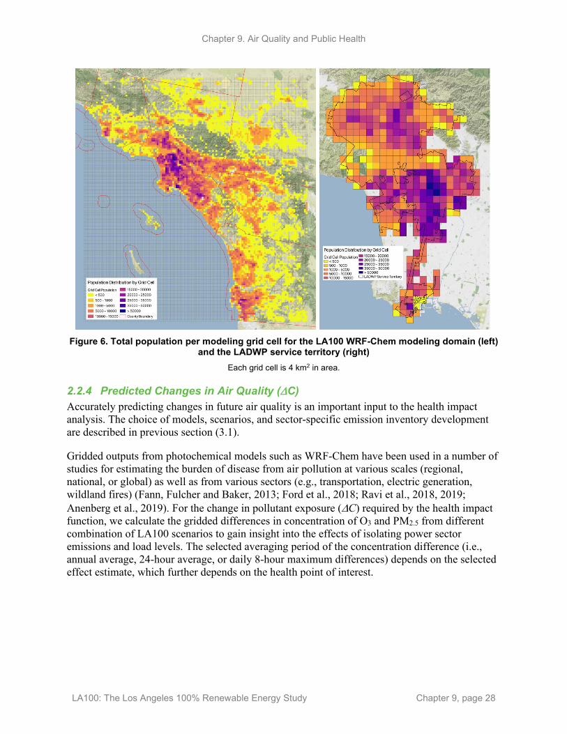
Chapter 9. Air Quality and Public Health
LA100: The Los Angeles 100% Renewable Energy Study Chapter 9, page 28
Figure 6. Total population per modeling grid cell for the LA100 WRF-Chem modeling domain (left)
and the LADWP service territory (right) Each grid cell is 4 km2 in area.
2.2.4 Predicted Changes in Air Quality (∆C) Accurately predicting changes in future air quality is an important input to the health impact analysis. The choice of models, scenarios, and sector-specific emission inventory development are described in previous section (3.1).
Gridded outputs from photochemical models such as WRF-Chem have been used in a number of studies for estimating the burden of disease from air pollution at various scales (regional, national, or global) as well as from various sectors (e.g., transportation, electric generation, wildland fires) (Fann, Fulcher and Baker, 2013; Ford et al., 2018; Ravi et al., 2018, 2019; Anenberg et al., 2019). For the change in pollutant exposure (∆C) required by the health impact function, we calculate the gridded differences in concentration of O3 and PM2.5 from different combination of LA100 scenarios to gain insight into the effects of isolating power sector emissions and load levels. The selected averaging period of the concentration difference (i.e., annual average, 24-hour average, or daily 8-hour maximum differences) depends on the selected effect estimate, which further depends on the health point of interest.
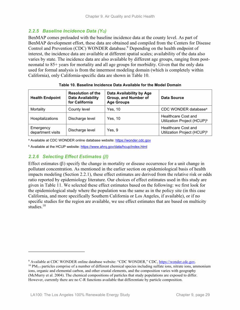
Chapter 9. Air Quality and Public Health
LA100: The Los Angeles 100% Renewable Energy Study Chapter 9, page 29
2.2.5 Baseline Incidence Data (YO) BenMAP comes preloaded with the baseline incidence data at the county level. As part of BenMAP development effort, these data are obtained and compiled from the Centers for Disease Control and Prevention (CDC) WONDER database.9 Depending on the health endpoint of interest, the incidence data are available at different spatial scales; availability of the data also varies by state. The incidence data are also available by different age groups, ranging from post-neonatal to 85+ years for mortality and all age groups for morbidity. Given that the only data used for formal analysis is from the innermost modeling domain (which is completely within California), only California-specific data are shown in Table 10.
Table 10. Baseline Incidence Data Available for the Model Domain
Health Endpoint Resolution of the Data Availability for California
Data Availability by Age Group, and Number of Age Groups
Data Source
Mortality County level Yes, 10 CDC WONDER databasea
Hospitalizations Discharge level Yes, 10 Healthcare Cost and Utilization Project (HCUP)b
Emergency department visits Discharge level Yes, 9 Healthcare Cost and
Utilization Project (HCUP)b
a Available at CDC WONDER online database website: https://wonder.cdc.gov b Available at the HCUP website: https://www.ahrq.gov/data/hcup/index.html
2.2.6 Selecting Effect Estimates (β) Effect estimates (β) specify the change in mortality or disease occurrence for a unit change in pollutant concentration. As mentioned in the earlier section on epidemiological basis of health impacts modeling (Section 2.2.1), these effect estimates are derived from the relative risk or odds ratio reported by epidemiology literature. Our choices of effect estimates used in this study are given in Table 11. We selected these effect estimates based on the following: we first look for the epidemiological study where the population was the same as in the policy site (in this case California, and more specifically Southern California or Los Angeles, if available), or if no specific studies for the region are available, we use effect estimates that are based on multicity studies.10
9 Available at CDC WONDER online database website: “CDC WONDER,” CDC, https://wonder.cdc.gov. 10 PM2.5 particles comprise of a number of different chemical species including sulfate ions, nitrate ions, ammonium ions, organic and elemental carbon, and other crustal elements, and the composition varies with geography (McMurry et al. 2004). The chemical compositions of particles that study populations are exposed to differ. However, currently there are no C-R functions available that differentiate by particle composition.

Chapter 9. Air Quality and Public Health
LA100: The Los Angeles 100% Renewable Energy Study Chapter 9, page 30
Table 11. Mortality and Morbidity HIF Used
Pollutant Category Health Endpoint Author Effect Estimate (b)a
Age Range Location
PM2.5
Long-term mortality All-cause mortality Krewski et al.
(2009) 0.0058 30–99 116 U.S. cities
Morbidity
Hospital admissions (all cardiovascular, less myocardial infarctions)
Moolgavkar (2000) 0.0014 18–64 Los
Angeles, CA
Hospital admissions (all cardiovascular, less myocardial infarctions)
Moolgavkar (2003) 0.0016 65–99 Los
Angeles, CA
Asthma ED visits Glad et al. (2012) 0.0039 0–99 Pittsburgh,
PA
Acute Myocardial Infarction (non-fatal)
Zanobetti et al. (2009) 0.0022 0–99 26 U.S.
communities
O3
Short-term mortality All-cause mortality
Zanobetti and Schwartz (2008)
0.0005 0–99 48 U.S. cities
Morbidity Asthma ED visitsb Glad et al. (2012) 0.0031 0–99 Pittsburgh,
PA
a These reported β coefficients are the mean value of effect estimates, but we will report a mean value with 95% confidence interval using the Monte-Carlo method. b There are no multicity studies for asthma ED visits; therefore, we select three different HIFs derived from three different studies. We will report values from all the studies.
2.3 Methods for Monetization of Benefits This section discusses methods for valuation, which refers to placing a monetary value on the estimated changes in health incidences described above. Improving air quality generally lowers the risk of an adverse health impact in the exposed population. Monetizing these health benefits depends on the society’s willingness to pay (WTP) for reduction in risk, or the cost of illness (COI) for a health effect. In the following subsections, we discuss our methods for monetizing the health benefits from a change in exposure to air pollutants, which includes both mortality and morbidity.
2.3.1 Monetization of Air Quality Health Effects This section describes the unit values that are available with the current version of BenMAP for the health endpoints modeled in the study. Different methods are used for valuing health endpoints. For mortality, the unit value used is the value of statistical life. For monetization of morbidity, the often-used unit value is based on based on WTP or COI. Details on these and unit values for morbidity and mortality are discussed in the following two sections.

Chapter 9. Air Quality and Public Health
LA100: The Los Angeles 100% Renewable Energy Study Chapter 9, page 31
2.3.2 Methods for Monetizing Morbidity Disease incidence can often result in emergency department visits, hospital admissions, and lost productivity. The total value to society of an individual’s avoidance of a hospital admission or emergency department visit can be thought of as having two components: (1) the COI to society, including the total medical costs plus the value of the lost productivity, as well as (2) the WTP of the individual, as well as that of others, to avoid the pain and suffering resulting from the illness. In the absence of estimates of social WTP to avoid hospital admissions for specific illnesses (components 1 plus 2), estimates of total COI (component 1) are available for use in BenMAP as conservative (lower bound) estimates.
Figure 7 shows a simple schematic of the approach for monetizing the morbidity benefits from an air pollution reduction scenario. Unit values for hospital admission and emergency department visits currently used in BenMAP are shown in Table 12. Unit values for hospital admissions are the total cost of illness and include hospital charges as well as lost wages due to hospital stays. BenMAP uses a county-specific median daily wage; therefore, the total cost of illness for hospital admissions varies from one county to another.
Figure 7. Approach for monetizing morbidity used in BenMAP
2.3.3 Methods for Monetizing Mortality In the economics literature, a concept called value of statistical life (VSL) is often used to quantify the benefits of avoiding a fatality. VSL is described as the willingness to pay (WTP) for a marginal reduction in risk of death in a society. VSL refers to value of statistical life, as opposed to the amount someone is willing to pay to avoid death. This idea is explained in Figure 8, which shows that each person in a population of 10,000 is willing to pay a certain amount to reduce the chances of death by one (hence a statistical life).

Chapter 9. Air Quality and Public Health
LA100: The Los Angeles 100% Renewable Energy Study Chapter 9, page 32
Figure 8. Approach for monetizing mortality in BenMAP
BenMAP uses data derived from 26 VSL estimates from economics literature that have been identified in the Section 812 Reports to Congress as “applicable to policy analysis.” For BenMAP, a distribution is fitted to the data from the 26 studies, and parameters for the distribution are derived (Table 12). The mean value of the distribution is used as a point estimate, with the distribution used to quantify uncertainty in the VSL. Although BenMAP output used 2015 U.S. dollars for calculating the monetized benefits, our results for all health endpoints are presented in 2019 U.S. dollars to be consistent with other LA100 results, such as bulk and distribution costs.

Chapter 9. Air Quality and Public Health
LA100: The Los Angeles 100% Renewable Energy Study Chapter 9, page 33
Table 12. Available Mortality and Morbidity Valuation Functions in BenMAP Unit value distributions and the parameters are used for quantifying the uncertainty11
Health Endpoint
Basis for Estimate
Age Range
Unit Value (2015 $)
Distribution of Unit Value
Parameters of Distribution (P1 and P2)a
P1 ($) P2 ($)
Mortality VSL based on 26 studies 0–99 8.7 million Weibull 9.6 million 15.1
million
Hospital Admissions (all cardiovascular)
National Inpatient Sample database (2007)
18–64 46,000 — — —
65–99 43,000 — — —
Acute Myocardial Infarctions
Wittels (1990) 0–99
Medical cost of $187,530; opportunity cost varies with age
— — —
Asthma ED Visits
Stanford et al. (1999) 0–99 450 Normal 8.95 —
a These parameter values and number of parameters depend on the assumed statistical distribution. More details on the distribution are available from the BenMAP user manual available at https://www.epa.gov/sites/production/files/2015-04/documents/benmap-ce_user_manual_march_2015.pdf.
11 Valuation for hospital admissions is derived from a very large dataset that comprises approximately 90% of all hospital discharges in the country and provides best estimates of the mean value of hospital charges and length of stay with negligible standard error. Therefore, there is no statistical distribution associated with unit value of hospital admissions.

Chapter 9. Air Quality and Public Health
LA100: The Los Angeles 100% Renewable Energy Study Chapter 9, page 34
3 Results and Discussion 3.1 Air Quality
3.1.1 Emission Inventory for Baseline and Future Scenarios In this section, we present our emissions inventories for the baseline (in year 2012) and selected future scenarios (in year 2045) in Los Angeles. We focus on NOx emissions as an important anthropogenic precursor to ozone (and secondary PM2.5), and primary PM2.5 emissions as an important contributor to PM2.5 concentrations. These are also two pollutants that are markedly changed by the LA100 scenarios. Emission inventories of other pollutants including CO, SOx, VOC and NH3 are shown in Appendix B.
For absolute emissions, we use two significant figures to report the values if greater than 0.1; otherwise, we use one significant figure. For percentage changes, we report the value accurate to single digit unless it is smaller than 1% for which we use one significant figure.
3.1.1.1 NOx Emission Inventory Annually averaged daily NOx emissions in Los Angeles for all selected scenarios from LA100-influenced sources are shown in Figure 9 and Table 13. NOx mass emissions reported here are based on molecular weight of NO2 (i.e., NO2-equivalent). (Note that “LA100-influenced sources” refer to the source types that are altered in the selected LA100 scenarios and ignores other source types.)
When considering all LA100-influenced sources, NOx emissions from 2012 to 2045 decrease by 88%, 95%, 88%, and 95% from Baseline (2012) to SB100 – Moderate, SB100 – High, Early & No Biofuels – Moderate, and Early & No Biofuels – High, respectively.
In Baseline (2012), LDVs are the largest contributor (52%) to LA100-related emissions, followed by the Ports12 (24%). However, in year 2045 for SB100 – Moderate and Early & No Biofuels – Moderate, emissions from residential buildings become the largest LA100-related source type (34% and 35% of LA100-related emissions, respectively) because of larger reductions (relative to 2012) in NOx from LDVs and the Ports. In SB100 – High and Early & No Biofuels – High, the Ports become the largest source of NOx (43% and 45% of LA100-influenced emissions, respectively). Recall that differences in electrification between the moderate and high electrification scenarios is larger for LDVs and buildings compared to the Ports (see Table 6 to Table 8). This leads to larger decreases in NOx for LDVs and buildings than the Ports when moving from moderate to high electrification level.
LADWP-owned power plants emit 0.54 metric tons/day of NOx in Baseline (2012), which decreases by 72% in SB100 – Moderate and SB100 – High mostly due to reductions in natural gas combustion. NOx emissions from LADWP-owned power plants are 88% and 84% lower for Early & No Biofuels – Moderate, and Early & No Biofuels – High relative to SB100 – Moderate and SB100 – High, respectively, due to replacement of natural gas with hydrogen at LADWP-
12 Recall that “the Ports” refers to the ports of Los Angeles and Long Beach combined.

Chapter 9. Air Quality and Public Health
LA100: The Los Angeles 100% Renewable Energy Study Chapter 9, page 35
owned power plants. Table 14 lists detailed annual total NOx emissions generated from LADWP-owned power plants by fuel technology types.
Emissions from school buses and urban buses contribute to 10% of LA100-influenced sources in Baseline (2012) and decrease to zero in all selected future scenarios in year 2045 due to 100% electrification (see Table 13). Emissions from commercial buildings decrease by 4% from Baseline (2012) to SB100 – Moderate and Early & No Biofuels – Moderate; though natural gas consumption increases, reduced emission factors are a more influential factor. In addition, emissions decrease by 98% from Baseline (2012) to SB100 – High and Early & No Biofuels – High.
Figure 9 also shows the fraction of emissions from LA100-influenced sources to all anthropogenic NOx emissions in Los Angeles (see the percentages above each bar). The reduction in this fraction from Baseline (2012) (34%) to SB100 – Moderate (10%) is due to the combined effect of increased electrification and reduced emission factors. This fraction is relatively small in all selected future LA100 scenarios. When comparing among selected future LA100 scenarios, the fraction is higher for SB100 – Moderate (Early & No Biofuels – Moderate) relative to SB100 – High (Early & No Biofuels – High) because of the higher electrification in LA100-influenced emissions sources. NOx emissions from all sources (both LA100-influenced and non-LA100-influenced) are shown in Appendix B.
Figure 9. Annually averaged daily NOx emissions from LA100-influenced sources in Los Angeles
for all selected scenarios Emissions for the selected future scenarios (SB100 – Moderate, SB100 – High, Early & No Biofuels – Moderate and Early & No Biofuels – High) are projected to year 2045. The percentage above each bar represents the fractional contribution of emissions from LA100-affected sources to all anthropogenic sources. Note that ‘LADWP-owned Power Plants’ include all of those located in the South Coast Air Basin, not just in the city of LA.

Chapter 9. Air Quality and Public Health
LA100: The Los Angeles 100% Renewable Energy Study Chapter 9, page 36
Table 13. Annually Averaged Daily NOx Emissions (metric tons/day) from LA100-Influenced Sources in Los Angeles and Citywide Total Emissions for all Selected Scenarios
Percentages in the parentheses show the percentage contribution of emissions from an LA100-influenced source to citywide total emissions in a scenario. Future scenarios are projected to year 2045.
Panel (a)
LADWP-Owned Power Plants
The Ports of LA and LB
Residential Buildings
Commercial Buildings LDVs Buses
Baseline (2012) 0.54 (0.4%)
12 (8%)
6.2 (4%)
0.49 (0.3%)
27 (18%)
5.3 (4%)
SB100 – Moderate 0.15 (0.2%)
1.7 (3%)
2.2 (4%)
0.47 (0.8%)
1.8 (3%) 0
SB100 – High 0.15 (0.3%)
1.1 (2%)
0.41 (0.7%)
0.01 (0.02%)
0.88 (2%) 0
Early & No Biofuels – Moderate
0.02 (0.03%)
1.7 (3%)
2.2 (4%)
0.47 (0.8%)
1.8 (3%) 0
Early & No Biofuels – High
0.02 (0.04%)
1.1 (2%)
0.41 (0.7%)
0.01 (0.02%)
0.88 (2%) 0
Panel (b)
Total Emissions from LA100-influenced Sectors
Citywide Total Emissions
Baseline (2012) 52 150
SB100 – Moderate 6.3 60
SB100 – High 2.5 57
Early & No Biofuels – Moderate 6.2 50
Early & No Biofuels – High 2.4 56

Chapter 9. Air Quality and Public Health
LA100: The Los Angeles 100% Renewable Energy Study Chapter 9, page 37
Table 14. Annual Total NOx Emissions (metric tons/year) Generated from LADWP-Owned Power Plants Located in the South Coast Air Basin by Fuel Technology Types
Percentages in the parentheses show the fractional change compared to the 2012 Baseline.
Fuel Technology
2012 Emissions for Baseline (metric tons)
2045 Emissions for SB100 – Moderate (metric tons)
2045 Emissions for SB100 – High (metric tons)
2045 Emissions for Early & No Biofuels – Moderate (metric tons)
2045 Emissions for Early & No Biofuels – High (metric tons)
Natural Gas Combined Cycle
199 (including all types of power plants)
30 31 0 0
Natural Gas Combustion Turbine
26 24 0 0
H2 Combustion Turbine
0 0 0.004 6.6 8.6
Total 199 56 (-72%) 55 (-72%) 6.6 (-97%) 8.6 (-96%)
3.1.1.2 PM2.5 Emission Inventory Annually averaged, daily primary PM2.5 emissions in Los Angeles for all selected scenarios from LA100-influenced sources are shown in Figure 10 and Table 15.
When considering all LA100-influenced sources, PM2.5 emissions from 2012 to 2045 decrease by 38%, 61%, 38%, and 62% from Baseline (2012) to SB100 – Moderate, SB100 – High, Early & No Biofuels – Moderate, and Early & No Biofuels – High, respectively.
Among all LA100-influenced sources, LDVs are the largest source-type for PM2.5 emissions in all selected scenarios. LDVs contribute 54% of PM2.5 from LA100-influenced sources in Baseline (2012), ~67% in SB100 – Moderate and Early & No Biofuels – Moderate in year 2045, and ~80% in SB100 – High and Early & No Biofuels – High. PM2.5 emissions from LDVs are generated from engine exhaust, and brake and tire wear as well. PM2.5 emissions from LDVs are reduced by 23% and 42% from Baseline (2012) in scenarios using Moderate electrification and High electrification, respectively.
Residential buildings are the second-largest contributor of PM2.5 from LA100-influenced sources in Baseline (2012). Emissions from residential buildings are reduced by 40% and 89% from Baseline (2012) to selected future scenarios with Moderate and High electrification, respectively.
PM2.5 emissions from the Ports contribute 12% of LA100-influenced emissions in Baseline (2012). Emissions from the Ports decrease by 66% from Baseline (2012) to Moderate electrification due to the adoption of 2017 Clean Air Action Plan, and they decrease by 31% from Moderate to High electrification due to increases in OGV shore power usage.
Emissions from urban and school buses make up 6% of LA100-influenced PM2.5 emissions in Baseline (2012) and decrease by 69% from Baseline (2012) to all four selected future scenarios
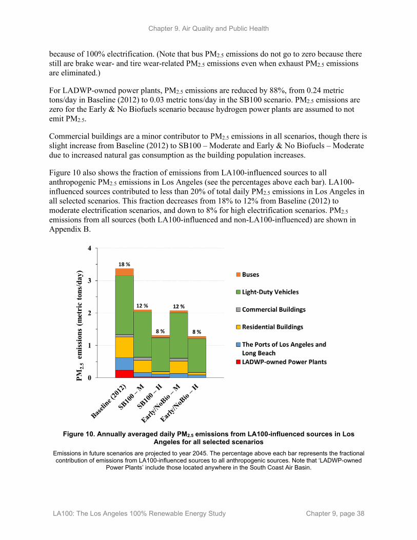
Chapter 9. Air Quality and Public Health
LA100: The Los Angeles 100% Renewable Energy Study Chapter 9, page 38
because of 100% electrification. (Note that bus PM2.5 emissions do not go to zero because there still are brake wear- and tire wear-related PM2.5 emissions even when exhaust PM2.5 emissions are eliminated.)
For LADWP-owned power plants, PM2.5 emissions are reduced by 88%, from 0.24 metric tons/day in Baseline (2012) to 0.03 metric tons/day in the SB100 scenario. PM2.5 emissions are zero for the Early & No Biofuels scenario because hydrogen power plants are assumed to not emit PM2.5.
Commercial buildings are a minor contributor to PM2.5 emissions in all scenarios, though there is slight increase from Baseline (2012) to SB100 – Moderate and Early & No Biofuels – Moderate due to increased natural gas consumption as the building population increases.
Figure 10 also shows the fraction of emissions from LA100-influenced sources to all anthropogenic PM2.5 emissions in Los Angeles (see the percentages above each bar). LA100-influenced sources contributed to less than 20% of total daily PM2.5 emissions in Los Angeles in all selected scenarios. This fraction decreases from 18% to 12% from Baseline (2012) to moderate electrification scenarios, and down to 8% for high electrification scenarios. PM2.5 emissions from all sources (both LA100-influenced and non-LA100-influenced) are shown in Appendix B.
Figure 10. Annually averaged daily PM2.5 emissions from LA100-influenced sources in Los
Angeles for all selected scenarios Emissions in future scenarios are projected to year 2045. The percentage above each bar represents the fractional contribution of emissions from LA100-influenced sources to all anthropogenic sources. Note that ‘LADWP-owned
Power Plants’ include those located anywhere in the South Coast Air Basin.

Chapter 9. Air Quality and Public Health
LA100: The Los Angeles 100% Renewable Energy Study Chapter 9, page 39
Table 15. Annually Averaged Daily PM2.5 Emissions (metric tons/day) from LA100-Influenced Sources and Citywide Total Emissions in Los Angeles for all Selected Scenarios
Percentages in the parentheses show the percentage contribution of emissions from an LA100-influenced source to citywide total emissions in a scenario. (Emissions in future scenarios are projected to year 2045.)
Panel (a)
LADWP-Owned Power Plants
The Ports of LA and LB
Residential Buildings
Commercial Buildings LDVs Buses
Baseline (2012) 0.24 (1%)
0.39 (2%)
0.64 (3%)
0.07 (0.4%)
1.8 (10%)
0.21 (1%)
SB100 – Moderate
0.03 (0.2%)
0.13 (0.8%)
0.38 (2%)
0.09 (0.5%)
1.4 (8%)
0.07 (0.4%)
SB100 – High 0.03 (0.2%)
0.09 (0.6%)
0.07 (0.4%)
0.002 (0.01%)
1.0 (6%)
0.07 (0.4%)
Early & No Biofuels – Moderate
0 0.13 (0.8%)
0.38 (2%)
0.09 (0.5%)
1.4 (8%)
0.07 (0.4%)
Early & No Biofuels – High
0 0.09 (0.6%)
0.07 (0.4%)
0.002 (0.01%)
1.0 (6%)
0.07 (0.4%)
Panel (b)
Total Emissions from LA100-influenced Sectors
Citywide Total Emissions
Baseline (2012) 3.4 18
SB100 – Moderate
2.1 17
SB100 – High 1.3 16
Early & No Biofuels – Moderate
2.1 17
Early & No Biofuels – High
1.3 16
3.1.2 Simulated Air Quality for Baseline and Future Scenarios In this section, we present simulated daily maximum 8-hour average O3 and daily averaged PM2.5 concentrations for all selected scenarios in Los Angeles. Details on pollutant metrics and how they are regulated in the NAAQS are described in Section 2.1.6.
For absolute concentrations, we round the value to single digit if greater than 1; otherwise, we use one significant figure. For percentage changes, we report the value accurate to single digit unless it is smaller than 1%.

Chapter 9. Air Quality and Public Health
LA100: The Los Angeles 100% Renewable Energy Study Chapter 9, page 40
3.1.2.1 Ozone (O3) Concentration In this section, we present simulated ozone concentrations in Los Angeles for all selected scenarios. Given that ozone pollution in Los Angeles is typically a summertime problem, with the ozone season usually defined as May to September (SCAQMD, 2017), we focus on results from our July simulations as representative of the ozone season.
Table 16 shows daily maximum 8-hour average O3 concentrations averaged over the city of Los Angeles for July. There is a 5% increase from Baseline (2012) (43.8 ppb) to SB100 – Moderate (46.0 ppb) in year 2045. This increase in O3 concentrations occurs despite reductions in NOx emissions because Los Angeles is known to be in the “NOx-saturated” regime (i.e., the NOx/VOC ratio is relatively high) (Stockwell et al., 2011; Fujita et al., 2013). In this regime, reaction with NO2 is the main sink pathway for the hydroxyl radical (via formation of nitric acid), and thus decreases in NOx lead to increases in hydroxyl radical. Since hydroxyl radical is an important ozone precursor, reductions in NOx ultimately lead to increases in ozone. Similarly, daily maximum 8-hour average O3 concentrations are 0.2% higher in Early & No Biofuels – High relative to SB100 – Moderate, representing the combined effect of increased electrification and replacement of natural gas with hydrogen-fueled power plants. The isolated effect of replacing natural gas with hydrogen-fueled power plants has negligible (less than 0.01 ppb) impact on simulated citywide O3 concentrations (i.e., SB100 – Moderate vs. Early & No Biofuels – Moderate; SB100 – High vs. Early & No Biofuels – High). The isolated effect of moving from moderate to high electrification levels leads to increases in citywide daily maximum 8-hour average O3 of 0.1 ppb (0.2%) (SB100 – High vs. SB100 – Moderate; Early & No Biofuels – High vs. Early & No Biofuels – Moderate).
Figure 11 qualitatively shows how O3 concentrations respond to changes in NOx and VOC emissions. The O3 increases simulated here can be thought of as following line “A” downward in the figure; there are temporary increases in O3 until getting to sufficiently low NOx, at which point further NOx reductions lead to marked O3 reductions in Los Angeles (i.e., the NOx limited regime). Also, we could avoid these O3 increases on the path to O3 reductions by having simultaneous reductions in emissions of VOC as shown by line B. In addition, note that while there are increases in O3 concentrations as electrification is increased, NOx and VOC concentrations are decreased due to reductions in their emissions. These changes alone can yield health benefits from direct exposure to these pollutants, despite not being quantified in LA100’s public health analyses (see later sections of this chapter).
Spatial patterns of simulated daily maximum 8-hour average O3 in Los Angeles are shown in Figure 12 for Baseline (2012), and SB100 – Moderate minus Baseline (2012). A version further including Early & No Biofuels – High minus Baseline (2012) is in Appendix B. In Baseline (2012), the San Fernando Valley region has the highest simulated daily maximum 8-hour O3 concentration with a maximum of 60.4 ppb. For SB100 – Moderate minus Baseline (2012), most of Los Angeles shows increases in O3 concentrations while the western region of the San Fernando Valley (i.e., where the highest ozone concentrations occur in Baseline (2012)) show decreases in O3, indicating that this region is shifting from “NOx- saturated” regime to “NOx-limited” regime. Overall, the largest increase in daily maximum 8-hour O3 is 6.3 ppb, and the largest reduction is 2.5 ppb.

Chapter 9. Air Quality and Public Health
LA100: The Los Angeles 100% Renewable Energy Study Chapter 9, page 41
Figure 13 uses SB100 – Moderate as the reference case and shows comparisons of the other three selected future scenarios relative to SB100 – Moderate. The comparison of O3 concentrations in the innermost domain among future scenarios (2045) with SB100 – Moderate as the reference is in Appendix B. The spatial pattern of daily maximum 8-hour average O3 concentrations in SB100 – Moderate are similar to that in Baseline (2012); the highest concentrations are observed in the San Fernando Valley with a maximum of 60.6 ppb. O3 concentrations are nearly identical for SB100 – Moderate and Early & No Biofuels – Moderate (panel c), with the maximum difference being less than 0.001 ppb. This suggests that shifting from natural gas to hydrogen power plants could have negligible influence on O3 concentrations. SB100 – High minus SB100 – Moderate (i.e., moving from moderate to high electrification levels, panel b) shows increases in daily maximum 8-hour average O3 concentrations in most regions of Los Angeles (maximum increase = 0.3 ppb), with the exception of the western part of the San Fernando Valley (maximum reduction = 0.07 ppb). Early & No Biofuels – High minus SB100 – Moderate (panel d) has a similar spatial pattern to SB100 – High minus SB100 – Moderate (panel b), with maximum increase in O3 of 0.3 ppb and maximum reduction of 0.07 ppb. This indicates that differences in O3 concentrations among future scenarios could be dominated by the electrification levels of the emitting sources relative to removing natural gas power plants in the future.
Table 16. Simulated Spatial Average (over City of Los Angeles) Daily Maximum 8-hour Average O3 in July for all Selected Scenarios
Percentages in parentheses show the fractional change of future scenarios compared to Baseline (2012). Future scenarios use the projected emissions inventories for year 2045.
Scenarios Baseline (2012)
SB100 – Moderate SB100 – High
Early & No Biofuels – Moderate
Early & No Biofuels – High
O3 (ppb) 43.8 46.0 (+5%) 46.1 (+5%) 46.0 (+5%) 46.1 (+5%)

Chapter 9. Air Quality and Public Health
LA100: The Los Angeles 100% Renewable Energy Study Chapter 9, page 42
Figure 11. O3 isopleth diagram to illustrate how 8-hour O3 concentration design values (DV) at a
location in Los Angeles can change in response to decreases in NOx and VOC emissions (in units of tons per day)
Line A indicates a pathway of reducing only NOx emissions, line B indicates a pathway of reducing NOx and VOC emissions simultaneously, and line C indicates a pathway of reducing only VOC emissions. This figure is modified from a presentation at SCAQMD Scientific Technology Modeling and Peer Review (STMPR) meeting on Jan. 27, 2021,13 and it was provided by Sang-Mi Lee at SCAQMD. Note that this figure was created for another project using a different emission inventory, and thus is only for illustration.
13 Presentation slides: Sang-Mi Lee, Air Quality Trends in the Basin and Design Values (SCAQMD, 2021), http://www.aqmd.gov/docs/default-source/Agendas/STMPR-Advisory-Group/stmpr-presentations-meeting-jan27-2021.pdf?sfvrsn=8.

Chapter 9. Air Quality and Public Health
LA100: The Los Angeles 100% Renewable Energy Study Chapter 9, page 43
Figure 12. Spatial pattern of simulated July daily maximum 8-hour average O3 concentrations in
Los Angeles for (a) Baseline (2012), and (b) SB100 – Moderate minus Baseline (2012) Panel (b) depicts changes over time from the 2012 baseline to 2045 for our reference scenario (SB100 – Moderate)

Chapter 9. Air Quality and Public Health
LA100: The Los Angeles 100% Renewable Energy Study Chapter 9, page 44
Figure 13. Spatial pattern of simulated July daily maximum 8-hour average O3 in Los Angeles for (a) SB100 – Moderate, and differences between SB100 – Moderate and (b) SB100 – High, (c) Early
& No Biofuels – Moderate, and (d) Early & No Biofuels – High Panel (b) isolates the effect of electrification of LA100-influenced sectors. Panel (c) shows the effect of shifting
LADWP-owned power plants from natural gas to hydrogen. Panel (d) represents the combined effect of electrification and removing natural gas power plants.
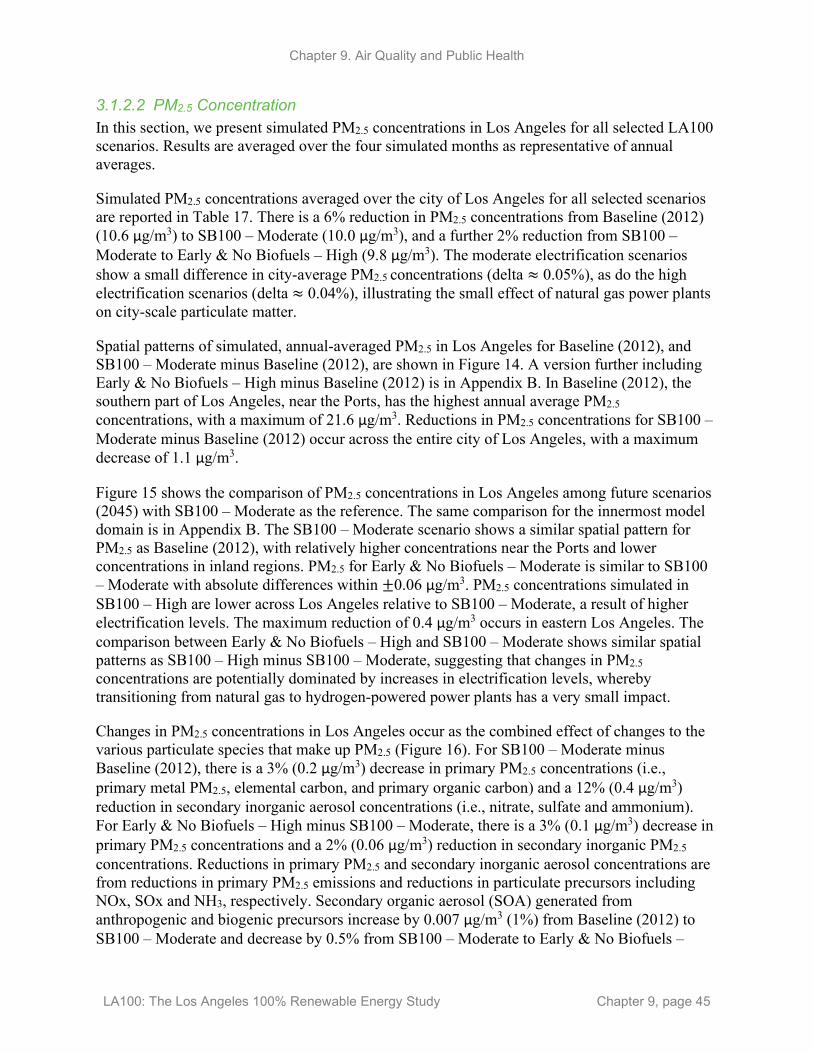
Chapter 9. Air Quality and Public Health
LA100: The Los Angeles 100% Renewable Energy Study Chapter 9, page 45
3.1.2.2 PM2.5 Concentration In this section, we present simulated PM2.5 concentrations in Los Angeles for all selected LA100 scenarios. Results are averaged over the four simulated months as representative of annual averages.
Simulated PM2.5 concentrations averaged over the city of Los Angeles for all selected scenarios are reported in Table 17. There is a 6% reduction in PM2.5 concentrations from Baseline (2012) (10.6 µg/m3) to SB100 – Moderate (10.0 µg/m3), and a further 2% reduction from SB100 – Moderate to Early & No Biofuels – High (9.8 µg/m3). The moderate electrification scenarios show a small difference in city-average PM2.5 concentrations (delta ≈ 0.05%), as do the high electrification scenarios (delta ≈ 0.04%), illustrating the small effect of natural gas power plants on city-scale particulate matter.
Spatial patterns of simulated, annual-averaged PM2.5 in Los Angeles for Baseline (2012), and SB100 – Moderate minus Baseline (2012), are shown in Figure 14. A version further including Early & No Biofuels – High minus Baseline (2012) is in Appendix B. In Baseline (2012), the southern part of Los Angeles, near the Ports, has the highest annual average PM2.5 concentrations, with a maximum of 21.6 µg/m3. Reductions in PM2.5 concentrations for SB100 – Moderate minus Baseline (2012) occur across the entire city of Los Angeles, with a maximum decrease of 1.1 µg/m3.
Figure 15 shows the comparison of PM2.5 concentrations in Los Angeles among future scenarios (2045) with SB100 – Moderate as the reference. The same comparison for the innermost model domain is in Appendix B. The SB100 – Moderate scenario shows a similar spatial pattern for PM2.5 as Baseline (2012), with relatively higher concentrations near the Ports and lower concentrations in inland regions. PM2.5 for Early & No Biofuels – Moderate is similar to SB100 – Moderate with absolute differences within ±0.06 µg/m3. PM2.5 concentrations simulated in SB100 – High are lower across Los Angeles relative to SB100 – Moderate, a result of higher electrification levels. The maximum reduction of 0.4 µg/m3 occurs in eastern Los Angeles. The comparison between Early & No Biofuels – High and SB100 – Moderate shows similar spatial patterns as SB100 – High minus SB100 – Moderate, suggesting that changes in PM2.5 concentrations are potentially dominated by increases in electrification levels, whereby transitioning from natural gas to hydrogen-powered power plants has a very small impact.
Changes in PM2.5 concentrations in Los Angeles occur as the combined effect of changes to the various particulate species that make up PM2.5 (Figure 16). For SB100 – Moderate minus Baseline (2012), there is a 3% (0.2 µg/m3) decrease in primary PM2.5 concentrations (i.e., primary metal PM2.5, elemental carbon, and primary organic carbon) and a 12% (0.4 µg/m3) reduction in secondary inorganic aerosol concentrations (i.e., nitrate, sulfate and ammonium). For Early & No Biofuels – High minus SB100 – Moderate, there is a 3% (0.1 µg/m3) decrease in primary PM2.5 concentrations and a 2% (0.06 µg/m3) reduction in secondary inorganic PM2.5 concentrations. Reductions in primary PM2.5 and secondary inorganic aerosol concentrations are from reductions in primary PM2.5 emissions and reductions in particulate precursors including NOx, SOx and NH3, respectively. Secondary organic aerosol (SOA) generated from anthropogenic and biogenic precursors increase by 0.007 µg/m3 (1%) from Baseline (2012) to SB100 – Moderate and decrease by 0.5% from SB100 – Moderate to Early & No Biofuels –

Chapter 9. Air Quality and Public Health
LA100: The Los Angeles 100% Renewable Energy Study Chapter 9, page 46
High. In addition, PM2.5 composition is nearly identical between SB100 – Moderate and Early & No Biofuels – Moderate, and between SB100 – High and Early & No Biofuels – High, again highlighting the very small role of converting LADWP-owned power plants from natural gas to hydrogen on city-scale PM2.5.
Table 17. Simulated PM2.5 Concentrations for all Selected Scenarios Averaged over the City of Los Angeles and the Four Simulated Months
Percentages in parentheses show the fractional change of future scenarios compared to Baseline (2012). Future scenarios use the projected emissions inventories for year 2045.
Scenarios Baseline (2012)
SB100 – Moderate
SB100 – High
Early & No Biofuels – Moderate
Early & No Biofuels – High
PM2.5 concentration (µg/m3) 10.6 10.0 (-6%) 9.8 (-8%) 10.0 (-6%) 9.8 (-8%)
Figure 14. Spatial pattern of PM2.5 concentrations in Los Angeles for (a) Baseline (2012), and (b)
SB100 – Moderate minus Baseline (2012) Values are averaged over the four simulated months to be representative of annual averages. Panel (b) depicts
changes over time from the 2012 baseline to 2045 for our reference scenario (SB100 – Moderate).
Chapter 9. Air Quality and Public Health
LA100: The Los Angeles 100% Renewable Energy Study Chapter 9, page 47
Figure 15. Spatial pattern of simulated PM2.5 concentrations in Los Angeles for (a) SB100 – Moderate, and differences between SB100 – Moderate and (b) SB100 – High, (c) Early & No
Biofuels – Moderate, and (d) Early & No Biofuels – High Values are averaged over the four simulated months to be representative of annual averages. Panel (b) isolates the effect of electrification of LA100-influenced sectors. Panel (c) shows the effect of shifting LADWP-owned power plants from removing natural gas generation. Panel (d) represents the combined effect of electrification and removing natural gas generation.

Chapter 9. Air Quality and Public Health
LA100: The Los Angeles 100% Renewable Energy Study Chapter 9, page 48
Figure 16. Contributions to citywide annual average PM2.5 concentrations (µg/m3) by species for all
selected scenarios
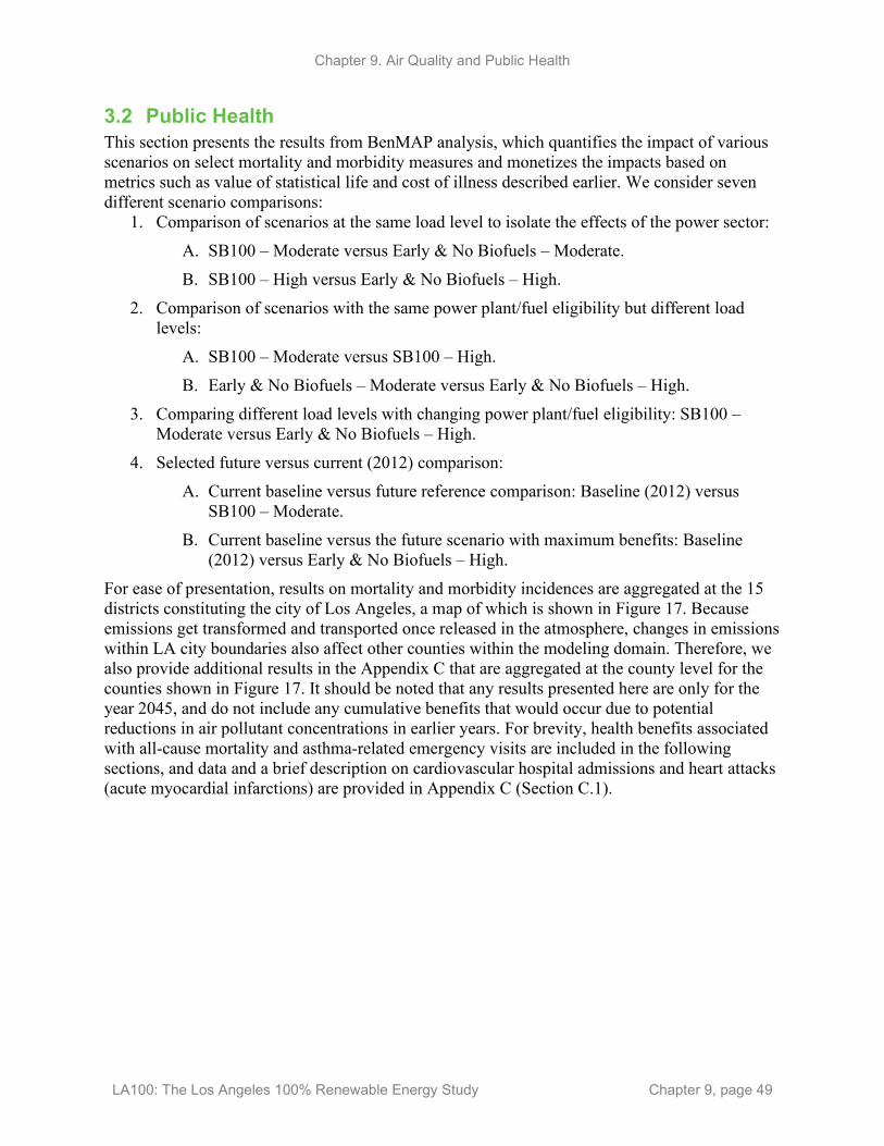
Chapter 9. Air Quality and Public Health
LA100: The Los Angeles 100% Renewable Energy Study Chapter 9, page 49
3.2 Public Health This section presents the results from BenMAP analysis, which quantifies the impact of various scenarios on select mortality and morbidity measures and monetizes the impacts based on metrics such as value of statistical life and cost of illness described earlier. We consider seven different scenario comparisons:
1. Comparison of scenarios at the same load level to isolate the effects of the power sector: A. SB100 – Moderate versus Early & No Biofuels – Moderate. B. SB100 – High versus Early & No Biofuels – High.
2. Comparison of scenarios with the same power plant/fuel eligibility but different load levels:
A. SB100 – Moderate versus SB100 – High. B. Early & No Biofuels – Moderate versus Early & No Biofuels – High.
3. Comparing different load levels with changing power plant/fuel eligibility: SB100 – Moderate versus Early & No Biofuels – High.
4. Selected future versus current (2012) comparison: A. Current baseline versus future reference comparison: Baseline (2012) versus
SB100 – Moderate. B. Current baseline versus the future scenario with maximum benefits: Baseline
(2012) versus Early & No Biofuels – High. For ease of presentation, results on mortality and morbidity incidences are aggregated at the 15 districts constituting the city of Los Angeles, a map of which is shown in Figure 17. Because emissions get transformed and transported once released in the atmosphere, changes in emissions within LA city boundaries also affect other counties within the modeling domain. Therefore, we also provide additional results in the Appendix C that are aggregated at the county level for the counties shown in Figure 17. It should be noted that any results presented here are only for the year 2045, and do not include any cumulative benefits that would occur due to potential reductions in air pollutant concentrations in earlier years. For brevity, health benefits associated with all-cause mortality and asthma-related emergency visits are included in the following sections, and data and a brief description on cardiovascular hospital admissions and heart attacks (acute myocardial infarctions) are provided in Appendix C (Section C.1).

Chapter 9. Air Quality and Public Health
LA100: The Los Angeles 100% Renewable Energy Study Chapter 9, page 50
Figure 17. Fifteen LA districts annotated by district number (left)
Counties that are wholly or partially contained in the modeling domain (shown in blue) are also shown (right, with county aggregated results reported in Appendix C).
3.2.1 Health Benefits Associated with Air Quality Changes in 2045
3.2.1.1 Impact of Changes to Power Supply In this subsection, we compare LA100 scenarios to isolate the air quality and health benefits associated with removing natural gas combustion in the power sector (and not allowing biofuels to be used to generate electricity at LADWP-owned power plants).
SB100 – Moderate versus Early & No Biofuels – Moderate Changes in the concentration of summertime O3 and reduction in the annual average concentration of PM2.5 in the Early & No Biofuels – Moderate scenario compared to the future baseline are shown in Figures 13 and 15, respectively. A comparison of these scenarios provides insight into air quality and health benefits when natural-gas-combusting power sector sources are removed, while keeping electrification at the Moderate level. Additional benefits from removal of natural gas combustion sources are quite small, with maximum PM2.5 reduction of about a tenth of a microgram per cubic meter. As a reference, the national ambient air quality standard (NAAQS) for PM2.5 is 12.0 µg/m3, and the Los Angeles region’s concentration (design value)14 exceeds the NAAQS by 2 µg/m3. July mean O3 concentration mostly decreases within LA, with a slight increase in southern parts of the city (districts 8 and 9; see Figure 17 for an annotated
14 The reported exceedance in concentration compared to NAAQS is based on the design value for the pollutants. Latest design value reports are available from the U.S. EPA website: “Air Quality Design Values,” EPA, https://www.epa.gov/air-trends/air-quality-design-values. Design values are also available: Kevin Durkee, Shoreh Cohanim, and Payam Pakbin, 2016 Air Quality Management Plan: Appendix II, Current Air Quality (SCAQMD, 2017), http://www.aqmd.gov/docs/default-source/clean-air-plans/air-quality-management-plans/2016-air-quality-management-plan/final-2016-aqmp/appendix-ii.pdf.

Chapter 9. Air Quality and Public Health
LA100: The Los Angeles 100% Renewable Energy Study Chapter 9, page 51
map of the City Council districts). However, these changes in O3 concentrations are very small and mostly within ± 0.1 ppb at any grid cell and this change is a small fraction of the spatial average of ozone concentration over the city of LA in SB100 – Moderate (46 ppb, see Table 16).
Given the very small changes in PM2.5 and O3 concentration from removal of natural gas combustion sources (and instead combusting hydrogen in the Early & No Biofuels – Moderate scenario), expected health benefits are small. About one premature mortality is avoided in the city, and the number of avoided ER visits due to asthma is less than one (Figure 18). These results indicate that the air quality and health impacts specific to this analysis of natural-gas-burning power sector sources are rather small, and maximum benefits are likely to occur close to and downwind of sources.
Figure 18. Health benefits due to air quality changes from the SB100 – Moderate to the Early & No
Biofuels – Moderate scenario are shown by avoided mortality (A) and ER visits (B) Avoided incidences from PM2.5 and O3 concentration changes as well as net benefits are shown. This comparison quantifies the benefits from changes in the power sector at moderate load (Early & No Biofuels – Moderate only allows hydrogen combustion whereas SB100 – Moderate allows for both hydrogen and natural gas to be burned at LADWP power plants in 2045, see Table 14). Early & No Biofuels – Moderate avoids one premature death in the city in 2045. (ER visits avoided are less than 1.)
SB100 – High versus Early & No Biofuels – High Both SB100 – High and Early & No Biofuels – High are scenarios with high energy efficiency and demand response, and high levels of electrification in the transportation sector (light-duty vehicles and buses only), buildings, and port of LA and Long Beach. A key difference between the scenarios is that natural-gas-based power sector sources are allowed in SB100 – High and not allowed in Early & No Biofuels – High.
Annual average concentration of PM2.5 is slightly higher in SB100 – High by about a tenth of a microgram per cubic meter. Similarly, O3 changes are small and within ± 0.1 ppb at any grid cell (change in pollutant concentration in these two future High load scenarios is similar to that shown for SB100 – Moderate versus Early & No Biofuels – Moderate in Figure 13 and Figure 15 for ozone and PM2.5, respectively). These differences in PM2.5 and ozone concentration in the two scenarios are very small compared to the citywide spatial average in the scenarios shown earlier in Table 16 and Table 17.
Health effects of natural gas power plants operation in the two high load electrification scenarios are shown in Figure 19. Given that natural gas plants are not large sources of PM2.5 and other

Chapter 9. Air Quality and Public Health
LA100: The Los Angeles 100% Renewable Energy Study Chapter 9, page 52
major sources emissions are constant in the two scenarios, associated health benefits are small and, in the case of PM2.5, fairly localized near the three natural gas power plants.
Figure 19. Health benefits due to air quality changes from the SB100 – High to the Early & No
Biofuels – High scenario Avoided incidences from PM2.5 and O3 concentration changes as well as net benefits are shown for both avoided
mortality (A) and ER visits (B). This comparison quantifies the benefits from changes in the power sector at high load (Early & No Biofuels – High scenario only allows hydrogen combustion whereas SB100 – High allows for both
hydrogen and natural gas to be burned at LADWP power plants in 2045, see Table 14). (There is a citywide net avoided death of 1, and an even smaller net benefit for ER visits.)
Insights from Comparisons of Two Power Plant Eligibility Criteria (SB100 and Early & No Biofuels) When Load Is Held Constant at Two Different Load Levels The previous two comparisons help us to isolate the air quality and health effects of natural gas plants when load is held constant at two different levels – Moderate and High. In each case emissions from non-power sectors are held constant at each load level. Not surprisingly, the two scenario comparisons do not differ greatly in terms of the expected benefits, and both reveal the same conclusion: natural gas plant operations associated with SB100 scenarios in 2045 do not affect air quality significantly compared to not allowing their use (i.e., in the Early & No Biofuels scenario), and thus does not produce significant public health benefits. Note that the comparison conducted is not the same as a comparison of the current operations of natural gas power plants in the city of LA; use of natural gas power plants under SB100 in 2045 is much lower than today (e.g., NOx emissions are reduced by 72%–97% depending on scenario (see Table 14), and combustion of hydrogen, the only allowed fuel in Early & No Biofuel scenarios, emits no PM2.5 or VOCs) . In summary, having no natural gas combustion in the power sector reduces mortality by one in the single modeling year (2045) and causes almost no change for asthma-related ER visits.
3.2.1.2 Impact of Changes due to Electrification of End Uses In this subsection, we discuss the expected air quality and health benefits when the power sector eligibility criteria are held constant (that is, the same technologies are allowed), but load levels are different for the scenarios compared. With these constraints, the scenario combinations are then SB100 – Moderate versus SB100 – High, and Early & No Biofuels – Moderate versus Early & No Biofuels – High.
Chapter 9. Air Quality and Public Health
LA100: The Los Angeles 100% Renewable Energy Study Chapter 9, page 53
SB100 – Moderate versus SB100 – High Compared to SB100 – Moderate, average annual PM2.5 concentration in SB100 – High is lower throughout the city, with maximum decrease reaching 0.5 µg/m3 (Figure 15). These largest reductions occur around the Port of LA and around the downtown area. As opposed to the impact of the power sector alone (discussed in Section 3.2.1.1) where the impact on PM2.5 was minimal, this PM2.5 concentration decrease is significant given that the LA region exceeds NAAQS by about 2 µg/m3, and the modeled reductions (0.2 µg/m3 or more for a large part of the city) can be significantly important for SOCAB’s targets to achieve attainment status. However, concentration of O3 increases in most parts of the city, with a maximum increase of 0.3 ppb occurring in grid cells near the Port of LA and downtown LA (Figure 13). As discussed earlier in the air quality section (Section 3.1.2), this increase is caused by nonlinearity in the chemistry of O3, where the direction of change not only depends on the direction of change for the primary precursor pollutants (NOx and VOCs), but also the state of atmosphere before any emission changes are introduced. The modeled increase in O3 is very small compared to the average citywide concentration in the two scenarios (~46 ppb, see Table 16).
Health benefits aggregated at the district level corresponding to changes in air quality for the two scenarios are shown in Figure 20. Maximum benefits are associated with a decrease in PM2.5 concentration, although the net benefits (due to both PM2.5 and O3) are slightly reduced because of increase in O3 concentration in SB100 – High scenario compared to SB100 – Moderate. Emissions reductions in SB100 – High result in approximately 53 avoided deaths (95% CI of 36–70) and reduce asthma-related ER visits by 19 (95% CI of -10–47) compared to SB100 – Moderate. Maximum benefits are expected in districts 1, 10, and 14 on the east end of the city.
Figure 20. Impacts of concentration change from SB100 – Moderate to SB100 – High scenario on avoided incidences of mortality (A) and ER visits (B) from changes in PM2.5 and O3 concentration
at the district level This comparison quantifies the benefits from high levels of electrification in end-use sectors compared to a moderate
level of electrification in the same sectors when emissions from combustion in LADWP-owned power plants are similar. (Citywide total of avoided premature deaths is 53 and 19 ER visits are avoided.)
Early & No Biofuels – Moderate versus Early & No Biofuels – High Reduction in the concentrations of summertime O3 and annual average PM2.5 the Early & No Biofuels – High relative to Early & No Biofuels – Moderate are similar to the SB100 – Moderate versus SB100 – High shown in Figure 13 and Figure 15, respectively. Compared to Early & No Biofuels – Moderate, the annual average PM2.5 in the Early & No Biofuels – High scenario

Chapter 9. Air Quality and Public Health
LA100: The Los Angeles 100% Renewable Energy Study Chapter 9, page 54
decreases by almost 0.5 µg/m3 in the center of the city, with the magnitude decreasing as one moves outwards from areas where emission reductions are high. Grid cells surrounding the ports of LA and Long Beach are also expected to see lower average annual concentration of PM2.5. As discussed in the previous subsection (comparing SB100 – Moderate versus SB100 – High), the decrease in concentration of PM2.5 from Early & No Biofuels – Moderate to Early & No Biofuels – High is significant and could be very helpful for attaining the PM2.5 NAAQS for the region. The direction of change is opposite for summertime O3, and the average of daily 8-hour maximum in July increases in Early & No Biofuels – Moderate compared to Early & No Biofuels – High. This increase in O3 is caused by the pollutant’s nonlinear chemistry, as discussed in more detail in the air quality section earlier in the chapter (see Section 3.1.2.1).
Aggregated health benefits for the 15 LA districts are shown in Figure 21, with the Early & No Biofuels – High scenario reducing citywide mortality by 52 (95% CI of 35–70) and ER visits by 18 (95% CI of -10–47) when compared to Early & No Biofuels – Moderate. Maximum benefits based on the two scenarios compared are expected in districts 1, 10, and 14 due to relatively larger PM2.5 concentration reduction and higher population density in these districts. District 15, which covers the Port of LA, does not see as much benefit despite high PM2.5 reductions in Early & No Biofuels – High because the area is sparsely populated. Given the relatively small increase in O3 concentration, net health benefits are positive for all the health endpoints considered.
Figure 21. Impacts of concentration change from the Early & No Biofuels – Moderate to Early & No Biofuels – High scenario on avoided incidences of mortality (A) and ER visits (B) from changes in
annual average PM2.5 and summertime O3 concentration for the 15 LA city council districts This comparison shows the benefits from high levels of electrification in end-use sectors compared to a moderate
level of electrification in the same sectors. Note that both Early & No Biofuel scenarios do not allow for combustion of natural gas in the LADWP-owned power plants in 2045, but hydrogen combustion is allowed. (Citywide total of
avoided deaths = 52, avoided ER visits = 18.)
Summary of Insights from High Level of Electrification in End-Use Sectors In previous subsection (Section 4.2.1.1), we saw that not operating natural gas power plants provides little air quality and health benefits at static load levels. Net air quality and health benefits increase significantly when one considers changes in other sectors, namely: increased electrification of light-duty vehicles and in the buildings sector (both residential and commercial buildings). Electrifying vehicles and buildings produced significant benefits in terms of reduced PM2.5 concentration as well as avoided mortality, with an average of 52 avoided premature deaths in the city. These results are of course in the context of a power sector transformed to
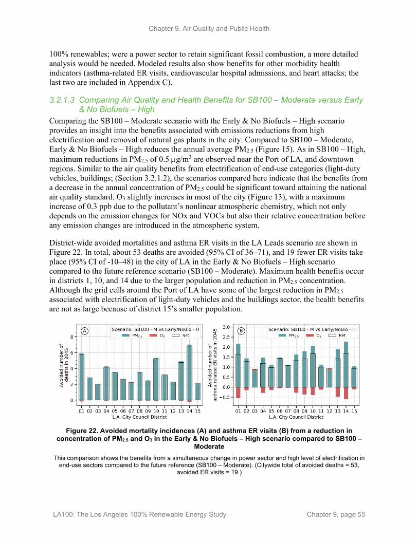
Chapter 9. Air Quality and Public Health
LA100: The Los Angeles 100% Renewable Energy Study Chapter 9, page 55
100% renewables; were a power sector to retain significant fossil combustion, a more detailed analysis would be needed. Modeled results also show benefits for other morbidity health indicators (asthma-related ER visits, cardiovascular hospital admissions, and heart attacks; the last two are included in Appendix C).
3.2.1.3 Comparing Air Quality and Health Benefits for SB100 – Moderate versus Early & No Biofuels – High
Comparing the SB100 – Moderate scenario with the Early & No Biofuels – High scenario provides an insight into the benefits associated with emissions reductions from high electrification and removal of natural gas plants in the city. Compared to SB100 – Moderate, Early & No Biofuels – High reduces the annual average PM2.5 (Figure 15). As in SB100 – High, maximum reductions in PM2.5 of 0.5 µg/m3 are observed near the Port of LA, and downtown regions. Similar to the air quality benefits from electrification of end-use categories (light-duty vehicles, buildings; (Section 3.2.1.2), the scenarios compared here indicate that the benefits from a decrease in the annual concentration of PM2.5 could be significant toward attaining the national air quality standard. O3 slightly increases in most of the city (Figure 13), with a maximum increase of 0.3 ppb due to the pollutant’s nonlinear atmospheric chemistry, which not only depends on the emission changes for NOx and VOCs but also their relative concentration before any emission changes are introduced in the atmospheric system.
District-wide avoided mortalities and asthma ER visits in the LA Leads scenario are shown in Figure 22. In total, about 53 deaths are avoided (95% CI of 36–71), and 19 fewer ER visits take place (95% CI of -10–48) in the city of LA in the Early & No Biofuels – High scenario compared to the future reference scenario (SB100 – Moderate). Maximum health benefits occur in districts 1, 10, and 14 due to the larger population and reduction in PM2.5 concentration. Although the grid cells around the Port of LA have some of the largest reduction in PM2.5 associated with electrification of light-duty vehicles and the buildings sector, the health benefits are not as large because of district 15’s smaller population.
Figure 22. Avoided mortality incidences (A) and asthma ER visits (B) from a reduction in
concentration of PM2.5 and O3 in the Early & No Biofuels – High scenario compared to SB100 – Moderate
This comparison shows the benefits from a simultaneous change in power sector and high level of electrification in end-use sectors compared to the future reference (SB100 – Moderate). (Citywide total of avoided deaths = 53,
avoided ER visits = 19.)

Chapter 9. Air Quality and Public Health
LA100: The Los Angeles 100% Renewable Energy Study Chapter 9, page 56
3.2.1.4 Comparison of Current (2012) versus Future (2045) Air Quality-Related Health Benefits
Here, we discuss the air quality and health benefits from future changes in air quality compared to the 2012 baseline. We use future reference (SB100 – Moderate) and the LA100 scenario with maximum emission reductions (Early & No Biofuels – High) and compare each to the Baseline (2012) in the following to quantify the health benefits.
Baseline (2012) versus SB100 – Moderate (2045,) A comparison of the historical baseline based on year 2012 data versus the future reference scenario – SB100 – Moderate – helps to understand differences from a number of different technological interventions to decrease emissions factors as well as any changes due to increased activity (driven by population and economic growth). It is important to note that many of the changes from 2012 to 2045 are not a result of the changes modeled in the power sector, light-duty vehicles, and buildings sectors within LA100. The difference in summertime change in daily average 8-hour O3 (based on the representative month of July) and annual concentration change for PM2.5 between the two scenarios are shown in in Figure 13 and Figure 15.
Within the city of LA, the annual average concentration of PM2.5 decreases by 0.5–1.0 µg/m3. These reductions may not seem significant, despite large controls on emission factors and reduced activity from some sources (e.g., fossil-fuel-based transportation), because other drivers (e.g., population, economic growth) spur activity, resulting in a smaller net decrease. Nevertheless, the concentration decrease should help the city in its goal of achieving the national ambient air quality standard for PM2.5, which it currently exceeds by about 2 µg/m3. There are, however, some regions in the northern part of LA and San Bernardino counties where the annual average PM2.5 concentration increases (see Figure 40 in Appendix B). The changing atmospheric chemical regime drives the changes in O3 concentration, with most urban areas in the modeling domain showing an increase in O3 concentration in the month of July in the SB100 – Moderate scenario (see Section 3.1.2.1 on ozone, for more discussion).
Resulting changes in PM2.5 and O3 induced all-cause mortality incidences and asthma-related ER visits are shown in Figure 23. About 96 deaths (95% CI of 67–130) are avoided in the SB100 – Moderate scenario compared to the 2012 baseline. Avoided deaths due to reduction in PM2.5 are largest in district 14, although this is also where maximum deaths due to an increase in O3 occur, which offsets some benefits from decreased concentration of PM2.5. In 2045, asthma-related ER visits increase in most districts due to an increase in O3 concentration. A total of 30 additional ER visits occur in 2045 (95% CI of 20–40) compared to 2012.

Chapter 9. Air Quality and Public Health
LA100: The Los Angeles 100% Renewable Energy Study Chapter 9, page 57
Figure 23. Changes in health impacts due to PM2.5 and O3 concentration changes in the SB100 –
Moderate scenario in 2045 compared to the Baseline in 2012, shown here for avoided mortality (A) and asthma caused ER visits (B)
This comparison quantifies the benefits from expected future changes under a reference scenario (SB100 – Moderate) compared to current (2012) atmospheric composition. (Citywide total of avoided deaths is 96, whereas ER
visits increase by 30.)
Baseline (2012) versus Early & No Biofuels – High (2045) A comparison of the baseline based on year 2012 emissions versus the Early & No Biofuels – High scenarios help to understand the effects of the future scenario with largest benefits for air quality and public health metrics considered.
Qualitatively, many of the observed differences in Early & No Biofuels – High (versus the 2012 Baseline) are similar to the previous subsection’s comparison of the 2012 Baseline with SB100 – Moderate. This is expected since the Early & No Biofuels – High scenario includes any emission reductions incorporated in the future reference scenario (SB100 – Moderate). Within the city of LA, the annual average concentration of PM2.5 decreases by 0.5–1.0 µg/m3, with some grid cells in the southern and eastern parts of the city seeing up to 1.5 µg/m3 reduction (see Figure 38 in Appendix B). As mentioned in the previous subsection, despite large controls on emission factors and reduced activity from some sources (e.g., fossil-fuel-based transportation), other drivers (e.g., population, economic growth) spur activity, thus there is a smaller decrease in PM2.5 concentrations. Comparing to the Baseline (2012) versus SB100 – Moderate comparison, once could clearly see further decrease in the concentration of PM2.5 in this scenario comparison, showing the impacts of emission reductions. Similar to the future reference scenario (SB100 – Moderate), changing atmospheric chemical regime drives the changes in O3 concentration, with most urban areas in the modeling domain showing an increase in O3 concentration in the representative summer month of July (see Figure 37, Appendix B).
Changes in the concentrations of PM2.5 and O3 are in opposite directions and the pollutant specific and net changes in the incidences of all-cause mortality and asthma-related ER visits are shown in Figure 24. In this scenario, total of 150 deaths (95% CI of 100–200) are avoided in the compared to the 2012 baseline. Notice that these avoided deaths are about 50% more than the SB100 – Moderate comparison to the current (2012 Baseline) scenario, and this is due to further reductions in the annual average PM2.5, especially in the densely populated eastern part of the city (such as district 14), which help to counter the ozone penalty observed in most parts of the city. In 2045, asthma-related ER visits increase in most districts due to an increase in O3

Chapter 9. Air Quality and Public Health
LA100: The Los Angeles 100% Renewable Energy Study Chapter 9, page 58
concentration. A total of 11 additional ER visits (95% CI of -51–27) occur in 2045 Early & No Biofuels – High scenario compared to 2012. Notice that fewer additional ER visits occur in this comparison compared to the SB100 – Moderate comparison presented earlier, and that is due to further decrease in PM2.5 concentrations in the Early & No Biofuels scenario.
Figure 24. Changes in health impacts due to PM2.5 and O3 concentration changes in the Early & No Biofuels – High scenario in 2045 compared to the 2012 baseline, shown here for avoided mortality
(A) and asthma caused ER visits (B) This comparison shows the benefits from a simultaneous change in power sector and high level of electrification in end-use sectors compared to the Baseline (2012). (Citywide total of avoided deaths is 150, whereas total ER visits
increase by 11.)
3.2.1.5 Summary of the Health Benefits The district-wise data and LA city total for avoided mean mortalities and 95% CI are shown in Table 18 for the seven scenarios compared. The number of avoided mortalities is similar when comparing SB100 – Moderate vs. SB100 – High, SB100 – Moderate vs. Early & No Biofuels – High, and Early & No Biofuels – Moderate vs. Early & No Biofuels – High, although slight differences do exist. In general, the scenarios where end-use sectors are electrified offer maximum health benefits. One should note that these health benefits are just for one year (2045) and do not include any benefits by implementing SB100 – Moderate related emission reduction measures. Thus, overall benefits compared to current pollution levels could be much higher, with cumulative benefits due to any emission reductions between now and 2045 likely to be much greater than those shown in Table 18.

Chapter 9. Air Quality and Public Health
LA100: The Los Angeles 100% Renewable Energy Study Chapter 9, page 59
Table 18. Avoided Incidences of All-Cause Mortality from the Seven Scenarios Compared Note that incidences for individual districts may not add up to the LA City total due to rounding.
Data in parentheses are the 95% confidence interval.
District
Isolating the effect of changes in power sector
Isolating the effect of changes in electrification of end -use sectors
Isolating the effect of simultaneous
changes in power sector and high end-
use electrification Future (2045) versus Baseline (2012)
comparison at two load levels
SB100 –Moderate versus Early & No Biofuels –Moderate
SB100 – High versus Early & No Biofuels – High
SB100 – Moderate versus SB100 –High
Early & No Biofuels –Moderate versus Early & No Biofuels – High
SB100 –Moderate versus Early & No Biofuels – High
Baseline (2012) versus SB100 –Moderate
Baseline (2012) versus Early & No Biofuels – High
01 0 (0 - 0) 0 (0 - 0) 6 (4 - 8) 6 (4 - 8) 6 (4 - 8) 8 (6 - 10) 14 (10 - 18)
02 0 (0 - 0) 0 (0 - 0) 3 (2 - 4) 3 (2 - 4) 3 (2 - 4) 6 (4 - 8) 9 (6 - 12)
03 0 (0 - 0) 0 (0 - 0) 2 (1 - 3) 2 (1 - 3) 2 (1 - 3) 6 (4 - 9) 8 (6 - 11)
04 0 (0 - 0) 0 (0 - 0) 4 (3 - 6) 4 (3 - 5) 4 (3 - 6) 7 (5 - 9) 11 (8 - 15)
05 0 (0 - 0) 0 (0 - 0) 3 (2 - 5) 3 (2 - 5) 3 (2 - 5) 6 (4 - 8) 9 (6 - 12)
06 0 (0 - 0) 0 (0 - 0) 3 (2 - 3) 3 (2 - 3) 3 (2 - 4) 7 (5 - 9) 9 (6 - 12)
07 0 (0 - 0) 0 (0 - 0) 2 (1 - 3) 2 (1 - 3) 2 (1 - 3) 6 (4 - 8) 9 (6 - 11)
08 0 (0 - 0) 0 (0 - 0) 3 (2 - 5) 3 (2 - 4) 3 (2 - 5) 5 (3 - 7) 8 (6 - 11)
09 0 (0 - 0) 0 (0 - 0) 2 (2 - 3) 2 (2 - 3) 2 (2 - 3) 3 (2 - 5) 6 (4 - 8)
10 0 (0 - 0) 0 (0 - 0) 5 (3 - 7) 5 (3 - 7) 5 (4 - 7) 6 (4 - 8) 11 (8 - 15)
11 0 (0 - 0) 0 (0 - 0) 3 (2 - 4) 3 (2 - 4) 3 (2 - 4) 4 (3 - 6) 8 (5 - 10)
12 0 (0 - 0) 0 (0 - 0) 2 (2 - 3) 2 (2 - 3) 2 (2 - 3) 7 (4 - 9) 9 (6 - 12)
13 0 (0 - 0) 0 (0 - 0) 5 (3 - 6) 5 (3 - 6) 5 (3 - 6) 7 (5 - 9) 12 (8 - 15)
14 0 (0 - 0) 0 (0 -0) 7 (5 - 9) 7 (5 - 9) 7 (5 - 9) 11 (8 - 14) 18 (12 - 23)
15 0 (0 - 0) 0 (0 - 0) 2 (1 - 3) 2 (1 - 3) 2 (1 - 3) 6 (4 - 8) 8 (5 - 10)
LA City 1 (1 - 1) 1 (0 - 1) 53 (35 - 70) 52 (35 - 70) 53 (36 - 71) 96 (67 - 130) 150 (100 - 200)

Chapter 9. Air Quality and Public Health
LA100: The Los Angeles 100% Renewable Energy Study Chapter 9, page 60
3.3 Monetization of Health Benefits The monetized value of the health benefits for the single modeling year (2045) for each LA district is shown in Figure 25 and Table 19. Avoided mortality in SB100 – High and Early & No Biofuels – High compared to the respective scenarios at lower load levels have similar monetized benefits, with the mean benefits of approximately $500 million in 2045. Given the uncertainty associated with the valuation distribution function (and the embedded uncertainty in health impact functions), the range of monetized benefits is large. However, the upper estimate of monetized benefits in these scenarios exceeds a billion dollars. Benefits based on a comparison of the two future scenarios show the effect of removing natural gas plants are a few million dollars in year 2045. It is also interesting to note that the districts on the east end of the city and central LA (districts 1, 10, 13 and 14) benefit most in the three scenario comparisons where one of the scenarios includes high electrification in end-use categories (LA city maps in middle two columns in Figure 25). These are the same districts where the future baseline (SB100 – Moderate) compared to the 2012 Baseline also shows maximum monetized benefits. This observed pattern is a combination of high population density (Figure 6) and relatively larger concentration change for these districts as seen in the concentration difference maps (Figures 12 - 15).
Figure 25. Monetized health benefits (in 2019 U.S. dollars) for the 15 LA City Council districts
across the LA100 scenarios compared Note that these benefits are in 2045 alone, and do not include any cumulative benefits for any of the scenarios
compared. Numeric data for individual districts are included in Table 19.
Chapter 9. Air Quality and Public Health
LA100: The Los Angeles 100% Renewable Energy Study Chapter 9, page 61
A comparison of the current Baseline (2012) and future reference (SB100 – Moderate) yield average annual monetized benefits of $900 million in 2045 and point to the benefits from air quality improvements in the future reference scenario compared to 2012. In the future, Early & No Biofuels – High yields maximum air quality improvements, and thus the corresponding air quality benefits are largest, and reach $1.4 billion compared to the 2012 baseline scenario. It should be noted that these benefits are for a single year: 2045 alone, as our modeling considered just one year. The expected monetized benefits could be much larger if integrated benefits due to any emission reductions between now and 2045 were to be considered, although predicting the magnitude of change is difficult given that the atmospheric sensitivity of pollutants could change during the course of emission changes. Benefits associated with other health endpoints (e.g., hospital admissions, emergency room visits) are much smaller, and the valuation of avoided mortality accounts for about 99% of the valuation shown in Table 19.

Chapter 9. Air Quality and Public Health
LA100: The Los Angeles 100% Renewable Energy Study Chapter 9, page 62
Table 19. Valuation of Annual Health Benefits from the Six Scenarios Compared (in $ Million, in 2019 U.S. dollars) These valuated benefits are just for the one modeling year (2045, except for the Baseline where the modeling year is 2012) and are not cumulative between now and the future.
Note that individual districts benefits may not add up to the city total due to rounding. Data in parentheses show the 95% confidence interval.
City District
Isolating the effect of changes in power sector
Isolating the effect of changes in electrification of end -use sectors
Isolating the effect of simultaneous
changes in power sector and high end-
use electrification Future (2045) versus Baseline (2012)
comparison at two load levels
SB100 –Moderate versus Early & No Biofuels –Moderate
SB100 – High versus Early & No Biofuels –High
SB100 –Moderate versus SB100 –High
Early & No Biofuels –Moderate versus Early & No Biofuels –High
SB100 –Moderate versus Early & No Biofuels –High
Baseline (2012) versus SB100 –Moderate
Baseline (2012) versus Early & No Biofuels –High
01 0 (0 - 1) 0 (0 - 1) 50 (1 - 150) 50 (1 - 150) 50 (1 - 150) 70 (-60 - 270) 130 (-60 - 420)
02 1 (0 - 2) 0 (0 - 1) 30 (1 - 70) 30 (1 - 70) 30 (1 - 70) 60 (-20 - 190) 90 (-20 - 260)
03 0 (0 - 0) 0 (0 - 1) 20 (2 - 50) 20 (2 - 50) 20 (2 - 50) 60 (5 - 170) 80 (7 - 220)
04 0 (0 - 1) 0 (0 - 1) 40 (1 - 110) 40 (1 - 110) 40 (1 - 110) 70 (-40 - 230) 110 (-40 - 340)
05 0 (0 - 1) 0 (0 - 1) 30 (2 - 90) 30 (2 - 90) 30 (2 - 90) 60 (-30 - 180) 90 (-30 - 270)
06 1 (0 - 2) 1 (0 - 2) 20 (2 - 70) 20 (2 - 70) 20 (2 - 70) 60 (-20 - 190) 90 (-10 - 260)
07 1 (0 - 2) 1 (0 - 2) 20 (2 - 50) 20 (1 - 50) 20 (2 - 60) 60 (-30 - 200) 80 (-30 - 250)
08 1 (0 - 3) 0 (0 - 1) 30 (1 - 90) 30 (1 - 90) 30 (1 - 90) 50 (-30 - 160) 80 (-20 - 250)
09 1 (0 - 2) 0 (0 - 1) 20 (0 - 60) 20 (0 - 60) 20 (0 - 60) 30 (-20 - 110) 60 (-20 - 170)
10 1 (0 - 2) 0 (0 - 1) 50 (1 - 140) 50 (1 - 130) 50 (1 - 140) 60 (-40 - 200) 110 (-40 - 340)
11 1 (0 - 2) 0 (0 - 1) 30 (2 - 80) 30 (2 - 80) 30 (2 - 80) 40 (-20 - 140) 70 (-20 - 220)
12 0 (0 - 1) 0 (0 - 1) 20 (2 - 60) 20 (2 - 60) 20 (2 - 60) 60 (-2 - 170) 80 (-0 - 230)
13 0 (0 - 1) 0 (0 - 1) 40 (0 - 120) 40 (0 - 120) 40 (0 - 130) 60 (-60 - 240) 110 (-60 - 360)
14 1 (0 - 2) 0 (-1 - 1) 60 (1 - 180) 60 (0 - 180) 60 (1 - 180) 100 (-90 -370) 170 (-90 - 550)
15 1 (0 - 2) 1 (0 - 2) 20 (1 - 50) 20 (1 - 50) 20 (1 - 60) 50 (-30 - 180) 70 (-20 - 230)
LA City 9 (1 - 20) 6 (-1 - 20) 500 (20 – 1,400) 500 (20 – 1,400) 500 (20 – 1,400) 900 (-480 – 3,000) 1,400 (-470 – 4,400)

Chapter 9. Air Quality and Public Health
LA100: The Los Angeles 100% Renewable Energy Study Chapter 9, page 63
4 Conclusion 4.1 Air Quality In this chapter, we present how LA100 scenario adoption could result in changes to air pollutant emissions (with a focus on NOx and PM2.5) and consequent changes in air quality (ozone and PM2.5 concentrations) for the city of Los Angeles.
Relative to the Baseline (2012) scenario, SB100 – Moderate (in year 2045) leads to an 88% and 38% reduction in annual NOx and PM2.5 emissions from LA100-influenced sectors in Los Angeles, respectively. This primarily occurs due to two factors: (a) increases in electrification of LA100-influenced sectors, and (b) assumed decreases in pollutant emission factors caused by policies outside the scope of LA100. Reduced emissions from LDVs and the Ports are the two major contributors to decreases in LA100-influenced NOx emissions and PM2.5 emissions.
Early & No Biofuels – High has 62% and 39% lower NOx and PM2.5 emissions relative to SB100 – Moderate, respectively, which is mostly attributable to increased electrification of LDVs and residential buildings. Comparing SB100 to Early & No Biofuels with constant electrification assumptions shows that shifting LADWP-owned power plants from natural gas to only hydrogen has a very small impact on citywide NOx and PM2.5 emissions relative to emissions from other LA100-influenced sources within the city. Emissions reductions from transitioning the LADWP-owned power plants to hydrogen are 0.1 and 0.03 metric tons/day for NOx and PM2.5, respectively.
The fraction of emissions from LA100-influenced sources to all anthropogenic NOx and PM2.5 emissions in Los Angeles decreases from Baseline (2012) (34% for NOx and 18% for PM2.5) to SB100 – Moderate (10% for NOx and 12% for PM2.5), and it decreases further to other selected future LA100 scenarios. This phenomenon suggests that LA100-influenced sources could contribute to a relatively small fraction of citywide total emissions.
Reductions in NOx emissions from Baseline (2012) to SB100 – Moderate lead to simulated increases in O3 concentrations for most parts of Los Angeles, with the citywide daily maximum 8-hour average O3 concentration increasing by 2.2 ppb (5%). This increase in O3 concentrations occurs despite reductions in NOx emissions because Los Angeles is known to be in the “NOx-saturated” regime. This effect is well known in the scientific community and is caused by the nonlinearities of ozone production; O3 concentrations increase when NOx emissions are decreased if the atmosphere has a higher ratio of NOx to VOCs. Despite of citywide increases in O3 concentration, decreases in O3 are simulated in a portion of the San Fernando Valley where baseline concentrations are highest, indicating that this region has shifted from “NOx-saturated” regime to “NOx-limited” regime. Spatial patterns in O3 changes for Early & No Biofuels – High minus SB100 – Moderate are similar to SB100 – Moderate minus Baseline (2012), with a citywide average increase of 0.1 ppb (Early & No Biofuels – High minus SB100 – Moderate), indicating that the role of high electrification outweighs removing natural gas power plants among LA100-influenced changes in shifting citywide O3 concentrations. Note that the primary and secondary National Ambient Air Quality Standard for 8-hour O3 concentrations is 70 ppb,

Chapter 9. Air Quality and Public Health
LA100: The Los Angeles 100% Renewable Energy Study Chapter 9, page 64
which is based on the annual fourth-highest daily maximum 8-hour concentration averaged over 3 years.
Reductions in PM2.5 emissions and other secondary PM2.5 precursors (e.g., NOx) result in reductions in PM2.5 concentrations across Los Angeles from Baseline (2012) to SB100 – Moderate, with citywide daily average PM2.5 concentration decreasing by 0.6 µg/m3 (6%). Early & No Biofuels – High showed PM2.5 concentrations that were 0.2 µg/m3 (2%) lower than SB100 – Moderate, which is primarily attributable to higher electrification level. Note that the primary NAAQS standard for annual mean (averaged over 3 years) PM2.5 concentration is 12.0 µg/m3.
Overall, our simulations suggest that the LA100 scenarios investigated in this chapter can lead to citywide reductions in PM2.5 concentrations and slight increases in O3 concentrations in Los Angeles. These changes in air pollution concentrations that result from the LA100 scenarios are dominated by increases in electrification. Transitioning LADWP-owned power plants from natural gas to hydrogen has a very small impact on city-scale air pollution. Reductions in PM2.5 concentrations induced by LA100 are beneficial for the city to meet the NAAQS. Increases in O3 concentrations are in the opposite direction to meet the NAAQS. However, the increase is relatively small compared to the current design value of Los Angeles (108 ppb), and this increase caused by reductions in NOx emissions is not unique to LA100. It is a general issue for the Los Angeles area because of the complexity of ozone chemistry and the state of the atmosphere in the South Coast Air Basin. This increase in O3 concentrations despite decreases in NOx emissions can be thought of as temporary “growing pains” on the path toward ultimately reducing O3 from decreasing NOx emissions in Los Angeles. Once NOx emissions get sufficiently low, further emissions decreases will lead to O3 reductions because the atmosphere will be in the “NOx-limited” regime. Alternatively, LA could avoid these O3 increases on the path to O3 reductions by having simultaneous reductions in emissions of VOC.
4.2 Public Health Benefits and their Monetization In this health benefits analysis, we estimate the avoided mortality and selected morbidity changes from various LA100 scenarios based on modeled changes in PM2.5 and O3 concentrations in 2045.
Our analysis suggests that the incidences of all-cause mortality and various disease (e.g., emergency department visits due to asthma, hospital admissions due to cardiovascular diseases) will decrease due to improvements in air quality caused by a reduction in emissions from various sectors affected by LA100 scenarios. We isolate the effects of changes in the power sector alone at two different load levels and find that irrespective of the load levels, net benefits from changes in the power sector are small, with an annual monetized value of health benefits of approximately a few million dollars in 2045.
A second set of scenario comparisons focused on assessing benefits under different levels of end-use electrification when the technology eligibility for the power sector is held constant. Here, we found that net benefits within the city are large due to changes in emissions in the buildings and transportation sectors. Average monetized benefits in 2045 associated with electrification of end uses are approximately $500 million in the city (in 2019$). Because the nature of air pollution is transboundary, emissions reductions within the city also affect the neighboring counties, and net monetized benefits exceed approximately $1 billion (2019$) in 2045 when considering health

Chapter 9. Air Quality and Public Health
LA100: The Los Angeles 100% Renewable Energy Study Chapter 9, page 65
benefits in neighboring counties; still, more than 80% of these benefits occur in LA County. These projected benefits could be additive to other projected benefits due to improvements in air quality likely to occur in the future from existing policies as projected by a comparison of Baseline (2012) with the future reference (SB100 – Moderate) scenario, which are approximately $900 million in 2045 for the City of LA and exceed approximately $4 billion when including neighboring counties in the modeling domain (in 2019$). The scenario with maximum air quality improvements (Early & No Biofuels – High) yields monetized benefits reaching approximately $1.4 billion (2019$) – and this comparison provides another estimate of benefits from decreased future emissions in 2045 relative to 2012. However, given the nonlinear chemical behavior of some pollutants and without detailed modeling analysis, it is hard to predict if these benefits from high electrification future scenarios (SB100 – High, Early & No Biofuels – High) could simply be added to the SB100 – Moderate benefits (compared to the 2012 Baseline). Similarly, cumulative co-benefits from any emissions control measures between now and the study horizon years could vary and will depend on the evolution of the state of the atmosphere in these intermediate years—but are expected to be much larger than the 2045 benefits shown here, which are based on just one year of modeling analysis.

Chapter 9. Air Quality and Public Health
LA100: The Los Angeles 100% Renewable Energy Study Chapter 9, page 66
5 Important Caveats 1. The focus of this chapter is on regional air pollution. It is not an exhaustive
environmental hazards analysis. For example, we do not investigate near-source exposures to emissions sources (e.g., power plants, freeways, the Ports), or fuel leaks. We did not investigate the role of transitioning LADWP-owned power plants to 100% renewable on near-source exposure to pollutants in 2045.15 In addition to the pollutants that were considered in this report (O3 and PM2.5), many other pollutants are emitted from combustion sources that can affect local air quality. These pollutants could be investigated in future work to develop estimates of additional health benefits to neighboring communities to LADWPs current natural-gas-fired power plants.
2. There are several limitations to the focus on regional air pollutants and their health effects in 2045 worth describing here. Each considered individually and also considered collectively lead to underestimation of the health benefits and monetized value of those benefits compared to those that would be experienced by Los Angeles residents as a result of the LA100 scenarios.
A. For evaluation of LA100 scenarios on regional air quality and their health impact, this analysis quantifies benefits based on just one year of modeling (2045) whereas net benefits will be cumulative. The magnitude of cumulative benefits depends on the pathway to 100% renewable energy. These cumulative benefits are likely to be much larger than the 2045 annual benefits, but their quantification will require further analysis of intermediate years. Such analysis could also help to identify pathways that maximize cumulative human health benefits.
B. Furthermore, the health benefits estimated here are just a subset of all health effects that result from exposure to O3 and PM2.5. For instance, other respiratory illnesses such a bronchitis are affected by air pollution exposure.
C. In addition, we only model two pollutants’ concentrations; many more will be affected by LA100 scenarios. For instance, NOx emissions were modeled for their importance to formation of O3 and PM2.5 in the atmosphere, yet exposure to NO2 also has direct health effects that were not modeled. These more local pollutants could be investigated using different air quality models to develop estimates of additional health benefits to neighboring communities to LADWP’s current natural gas-fired power plants.
D. Finally, air quality and its effect on public health is evaluated only in terms of ambient (outdoor) air pollutant concentration, not considering changes to indoor air quality. Indoor air quality and its health effects from changes in gas usage within homes as well as how indoor pollutant concentrations changes due to changes to outdoor concentration via ventilation are not evaluated here.
15 Early & No Biofuels eliminates the use of natural gas at LADWP-owned facilities, instead exclusively using hydrogen for limited hours required to maintain reliability. The SB100 scenario allows limited use of natural gas (offset through renewable energy credits), though much lower today’s usage.

Chapter 9. Air Quality and Public Health
LA100: The Los Angeles 100% Renewable Energy Study Chapter 9, page 67
3. In this study, we strove to assess the impacts of emissions changes on air pollutant concentrations in Los Angeles. To avoid including additional confounding factors, we keep the same meteorological year across all scenarios in air quality modeling. The 2045 scenarios are driven by 2012 meteorology, consistent with the selection of Baseline year. Thus, the potential effects of changes to the climate are not considered. Climate change is expected to lead to additional changes in air pollutant concentrations through impacting (a) temperature-sensitive emissions of air pollutant precursors (e.g., emissions of volatile organic compounds), (b) temperature-sensitive chemical reaction rates, (c) phase-partitioning of semi-volatile species, which can lead to particle-phase pollutants moving to the gas-phase at higher temperatures, and (d) future changes in meteorological variables that impact removal of pollutants from Los Angeles (e.g., winds and precipitation). There remains uncertainty on the net effect of these various pathways on air pollution. Future analysis could consider simultaneous impacts from climate change on air quality and subsequent health impacts.
4. The focus of this chapter is to quantify the impacts of emission reductions on citywide air quality due to selected future LA100 scenarios. Given that the response of air pollutant concentrations to emissions changes is dependent on the baseline state of the atmosphere, we needed to decide whether to prioritize focusing on changes in air pollutant concentrations using (a) the 2012 baseline as a base case, or (b) the reference scenario SB100 – Moderate as a base case. For (a) we would have used 2012 emissions as a starting point and then modified those emissions using only LA100-influenced emissions reductions. For (b) we would start with 2012 as a baseline but include expected changes to emissions outside the scope of LA100 for a more realistic atmospheric state in 2045. Ultimately, we chose (b) so that we could isolate the effects of electrification and removing natural gas power plants in the context of a more realistic atmospheric state for 2045. However, this implies that comparisons for 2045 versus 2012 include changes in emissions outside the scope of LA100.
5. Relatedly, air quality results shown here are highly dependent on the ways that the scenarios were defined. Simulated ozone responses to emissions reductions are highly dependent on atmospheric context, and thus scenarios investigated. This is true both the projection scenarios, and the reference scenario used as a point of comparison. Investigating projections with larger NOx reductions could potentially have led to simulated ozone decreases for all of Los Angeles.
6. In addition, air quality modeling results shown here were designed for the purpose of demonstrating the potential changes in air quality induced by LA100 scenarios, rather than predict actual air pollutant concentrations in the future. The comparison of air pollutant concentrations between scenarios can illustrate the combined or isolated effect of electrification levels and power plant eligibility in LA100. However, we do not recommend comparing the simulated air pollutant concentrations directly with the National Ambient Air Quality Standards.
7. Note that the contribution of LA100-influenced sources to citywide total emission could be relatively small in the future (indicated by the percent labels over each column in Figure 1), and that including additional emissions reductions policies beyond LA100 would lead to greater emissions reductions. For example, medium- and heavy-duty trucks are one of the largest sources of air pollutant emissions in Los Angeles. LA100 did not

Chapter 9. Air Quality and Public Health
LA100: The Los Angeles 100% Renewable Energy Study Chapter 9, page 68
include medium- and heavy-duty vehicles in the development of scenarios (outside the Ports), thus only already existing regulations were considered in the air quality modeling. If LA100 had developed electrification scenarios (or other zero-emission vehicle pathways) for medium- and heavy-duty vehicles, greater emission reductions than considered here would have been included. Similarly, we do not include any mandates requiring larger penetration of electric vehicles in California, such as the recent Executive Order N-79-20, which sets a target of 100 percent of in-state sales of new light-duty vehicles to be zero emissions by 2035. This new mandate, and others, would further reduce emissions and provide air quality benefits outside of what is modeled here. Emissions reductions beyond current regulations from off-road sources (e.g., construction equipment, locomotives, airplanes, ships) are another category of contributors to air pollution that were not explicitly addressed in LA100 (outside the Ports).

Chapter 9. Air Quality and Public Health
LA100: The Los Angeles 100% Renewable Energy Study Chapter 9, page 69
6 References Ackermann, I. J. et al. 1998. Modal Aerosol Dynamics Model for Europe: Development and First Applications,” Atmospheric Environment, 32 (17): 2981–2999. doi: 10.1016/S1352-2310(98)00006-5.
Ahmadov, R. et al. 2012. “A Volatility Basis Set Model for Summertime Secondary Organic Aerosols over the Eastern United States in 2006,” Journal of Geophysical Research: Atmospheres, 117 (D6), p. n/a-n/a. doi: 10.1029/2011JD016831.
Anenberg, S. C. et al. 2019. “The Global Burden of Transportation Tailpipe Emissions on Air Pollution-Related Mortality in 2010 and 2015,” Environmental Research Letters, 14 (9), p. 094012. doi: 10.1088/1748-9326/ab35fc.
Bell, M. L. et al. 2004. “Ozone and Short-term Mortality in 95 US Urban Communities, 1987-2000,” JAMA, 292 (19): 2372–2378. doi: 10.1001/jama.292.19.2372.
Boylan, J. W., and A. G. Russell. 2006. “PM and Light Extinction Model Performance metrics, Goals, and Criteria for Three-Dimensional Air Quality Models,” Atmospheric Environment, 40 (26): 4946–4959. doi: 10.1016/j.atmosenv.2005.09.087.
California Air Resources Board 2017. Emission Inventory Activities. https://ww2.arb.ca.gov/emission-inventory-activities (Accessed: 17 January 2021).
California Air Resources Board (n.d.) EMFAC2014 Web Database, 2014. https://arb.ca.gov/emfac/2014/ (Accessed: 17 January 2021).
Carter, W. P. L. 2003 The SAPRC-99 Chemical Mechanism and Updated VOC Reactivity Scales.
Chen, D. et al. 2013. “WRF-Chem Simulation of NOx and O3 in the L.A. Basin during CalNex-2010,” Atmospheric Environment, 81: 421–432. doi: 10.1016/j.atmosenv.2013.08.064.
Chen, F. et al. 2001. “Coupling an Advanced Land Surface–Hydrology Model with the Penn State–NCAR MM5 Modeling System. Part I: Model Implementation and Sensitivity,” Monthly Weather Review, 129 (4): 569–585. doi: 10.1175/1520-0493 (2001)129<0569:CAALSH>2.0.CO;2.
Chen, F. et al. 2011. “The Integrated WRF/Urban Modelling System: Development, Evaluation, and Applications to Urban Environmental Problems,” International Journal of Climatology, 31 (2): 273–288. doi: 10.1002/joc.2158.
Ching, J. et al. 2009. “National Urban Database and Access Portal Tool,” Bulletin of the American Meteorological Society, 90 (8): 1157–1168. doi: 10.1175/2009BAMS2675.1.
Chou, M.-D., and M. J. Suarez. 1999. Technical Report Series on Global Modeling and Data Assimilation Volume 15: A Solar Radiation Parameterization for Atmospheric Studies. 1st edn. Edited by M. J. Suarez. Maryland. doi: TM-1999-104606,Vol 15.

Chapter 9. Air Quality and Public Health
LA100: The Los Angeles 100% Renewable Energy Study Chapter 9, page 70
Dockery, D. W. et al. 1993. “An Association between Air Pollution and Mortality in Six U.S. Cities,” New England Journal of Medicine, 329 (24): 1753–1759. doi: 10.1056/NEJM199312093292401.
Dyer, A. J., and B. B. Hicks. 1970. “Flux‐Gradient Relationships in the Constant Flux Layer,” Quarterly Journal of the Royal Meteorological Society, 96 (410): 715–721. doi: 10.1002/QJ.49709641012.
Emmons, L. K. et al. 2010. “Description and Evaluation of the Model for Ozone and Related Chemical Tracers, Version 4 (MOZART-4),” Geoscientific Model Development, 3 (1): 43–67. doi: 10.5194/gmd-3-43-2010.
Fann, N., C. M. Fulcher, and K. Baker. 2013. “The Recent and Future Health Burden of Air Pollution Apportioned Across U.S. Sectors,” Environmental Science & Technology, 47 (8): 3580–3589. doi: 10.1021/es304831q.
Ford, B. et al. 2018. “Future Fire Impacts on Smoke Concentrations, Visibility, and Health in the Contiguous United States,” GeoHealth, 2 (8): 229–247. doi: 10.1029/2018GH000144.
Fry, J. et al. 2011. “Completion of the 2006 National Land Cover Database for the Conterminous United States,” Photogrammetric Engineering and Remote Sensing, 77 (9): 858–864.
Fujita, E. M. et al. 2013. “Past and Future Ozone Trends in California’s South Coast Air Basin: Reconciliation of Ambient Measurements with Past and Projected Emission Inventories) Past and Future Ozone Trends in California’s South Coast Air Basin: Reconciliation of Ambient Measurements with Past and Projected Emission Inventories,” Journal of the Air & Waste Management Association, 63 (1): 54–69. doi: 10.1080/10962247.2012.735211.
Gallagher, C. L., and T. Holloway. 2020. “Integrating Air Quality and Public Health Benefits in U.S. Decarbonization Strategies,” Frontiers in Public Health. Frontiers Media S.A. doi: 10.3389/fpubh.2020.563358.
Glad, J. A. et al. 2012. “The Relationship of Ambient Ozone and PM2.5 Levels and Asthma Emergency Department Visits: Possible Influence of Gender and Ethnicity,” Archives of Environmental & Occupational Health, 67 (2): 103–108. doi: 10.1080/19338244.2011.598888.
Gordis, L. 2004. Epidemiology. 3rd edn. Elsevier Saunders.
Grell, G. A. et al. 2005. “Fully Coupled “Online” Chemistry within the WRF Model,” Atmospheric Environment, 39 (37): 6957–6975. doi: 10.1016/J.ATMOSENV.2005.04.027.
Grell, G. A., and D. Dévényi. 2002 “A Generalized Approach to Parameterizing Convection Combining Ensemble and Data Assimilation Techniques,” Geophysical Research Letters, 29 (14): 38-1-38–4. doi: 10.1029/2002GL015311.
Hale, E. et al. 2018. The Demand-side Grid (dsgrid) Model Documentation. Golden, CO: National Renewable Energy Laboratory.

Chapter 9. Air Quality and Public Health
LA100: The Los Angeles 100% Renewable Energy Study Chapter 9, page 71
Hong, S.-Y. et al. 2006. “A New Vertical Diffusion Package with an Explicit Treatment of Entrainment Processes,” Monthly Weather Review, 134 (9): 2318–2341. doi: 10.1175/MWR3199.1.
ICF International and Energy Environmental Economics. 2014. California Transportation Electrification Assessment, Phase 1: Final Report. San Francisco, CA.
Kim, S.-W. et al. 2009. “NO 2 Columns in the Western United States Observed from Space and Simulated by a Regional Chemistry Model and their Implications for NO x Emissions,” Journal of Geophysical Research, 114 (D11), p. D11301. doi: 10.1029/2008JD011343.
Krewski, D. et al. 2009. “Extended Follow-Up and Spatial Analysis of the American Cancer Society Study Linking Particulate Air Pollution and Mortality,” Research Report (Health Effects Institute), (140): 5–114; discussion 115-136.
Kusaka, H. et al. 2001. “A Simple Single-Layer Urban Canopy Model for Atmospheric Models: Comparison with Multi-Layer and Slab Models,” Boundary-Layer Meteorology, 101 (3): 329–358. doi: 10.1023/A:1019207923078.
LADWP. 2019. “Emissions Reporting System”.
Li, Y. et al. 2019. “Effects of Urbanization on Regional Meteorology and Air Quality in Southern California,” Atmospheric Chemistry and Physics, 19 (7): 4439–4457. doi: 10.5194/acp-19-4439-2019.
Lin, Y.-L. et al. 1983. “Bulk Parameterization of the Snow Field in a Cloud Model,” Journal of Climate and Applied Meteorology, 22 (6): 1065–1092. doi: 10.1175/1520-0450(1983)022<1065:BPOTSF>2.0.CO;2.
Lippmann, M. 1989. “Health Effects Of Ozone A Critical Review,” Journal of the Air Pollution Control Association, 39 (5): 672–695. doi: 10.1080/08940630.1989.10466554.
Madronich, S. 1987. “Photodissociation in the Atmosphere: 1. Actinic Flux and the Effects of Ground Reflections and Clouds,” Journal of Geophysical Research, 92 (D8), p. 9740. doi: 10.1029/JD092iD08p09740.
Mann, J. K. et al. 2002. “Air Pollution and Hospital Admissions for Ischemic Heart Disease in Persons with Congestive Heart Failure or Arrhythmia.,” Environmental Health Perspectives, 110 (12): 1247–1252. doi: 10.1289/ehp.021101247.
Mesinger, F. et al. 2006. “North American Regional Reanalysis,” Bulletin of the American Meteorological Society, 87 (3): 343–360. doi: 10.1175/BAMS-87-3-343.
Mlawer, E. J. et al. 1997. “Radiative Transfer for Inhomogeneous Atmospheres: RRTM, a Validated Correlated-k Model for the Longwave,” Journal of Geophysical Research: Atmospheres, 102 (D14): 16663–16682. doi: 10.1029/97JD00237.
Chapter 9. Air Quality and Public Health
LA100: The Los Angeles 100% Renewable Energy Study Chapter 9, page 72
Moolgavkar, S. H. 2000. “Air Pollution and Hospital Admissions for Diseases of the Circulatory System in Three U.S. Metropolitan Areas,” 50, p. 9.
Moolgavkar, S. H. 2003. Air Pollution and Daily Deaths and Hospital Admissions in Los Angeles and Cook Counties. In: Revised Analyses of Time-Series Studies of Air Pollution and Health. Boston, MA: Health Effects Institute. https://www.healtheffects.org/system/files/TimeSeries.pdf (Accessed: 12 December 2020).
National Centers for Environmental Prediction. 2007. Global Forecast System Analysis Data Historical Archive at 0.5 Degree. https://www.ncdc.noaa.gov/data-access/model-data/model-datasets/global-forcast-system-gfs.
Ostro, B. D. et al. 1995. “Air Pollution and Asthma Exacerbations Among African-American Children in Los Angeles,” Inhalation Toxicology, 7 (5): 711–722. doi: 10.3109/08958379509014475.
Paulson, C. A. 1970. “The Mathematical Representation of Wind Speed and Temperature Profiles in the Unstable Atmospheric Surface Layer,” Journal of Applied Meteorology, 9 (6): 857–861. doi: 10.1175/1520-0450(1970)009<0857:TMROWS>2.0.CO;2.
Pope, C. A., and D. W. Dockery. 2006. “Health Effects of Fine Particulate Air Pollution: Lines that Connect,” Journal of the Air and Waste Management Association, 56 (6): 709–742. doi: 10.1080/10473289.2006.10464485.
Pope III, C. A. et al. 2004. “Cardiovascular Mortality and Long-Term Exposure to Particulate Air Pollution,” Circulation, 109 (1): 71–77. doi: 10.1161/01.CIR.0000108927.80044.7F.
Pope III, C. A., and D. W. Dockery. 2006. “Health Effects of Fine Particulate Air Pollution: Lines that Connect,” Journal of the Air & Waste Management Association, 56 (6): 709–742. doi: 10.1080/10473289.2006.10464485.
Ravi, V. et al. 2018. “Air Quality and Health Impacts of an Aviation Biofuel Supply Chain Using Forest Residue in the Northwestern United States,” Environmental Science & Technology, 52 (7): 4154–4162. doi: 10.1021/acs.est.7b04860.
Ravi, V. et al. 2019. “Impacts of Prescribed Fires and Benefits from their Reduction for Air Quality, Health, and Visibility in the Pacific Northwest of the United States,” Journal of the Air & Waste Management Association, 69 (3): 289–304. doi: 10.1080/10962247.2018.1526721.
Sacks, J. D. et al. 2018. “The Environmental Benefits Mapping and Analysis Program – Community Edition (BenMAP–CE): A Tool to Estimate the Health and Economic Benefits of Reducing Air Pollution,” Environmental Modelling & Software, 104: 118–129. doi: 10.1016/j.envsoft.2018.02.009.
San Pedro Bay Ports. 2017 San Pedro Bay Ports Clean Air Action Plan 2017. Los Angeles, CA.
South Coast Air Quality Management District. 2017. 2016 Air Quality Management Plan: Appendix III Base and Future Year Emission Inventory.

Chapter 9. Air Quality and Public Health
LA100: The Los Angeles 100% Renewable Energy Study Chapter 9, page 73
———. 201. Rule 1135. Emissions of Oxides of Nitrogen From Electricity Generating Facilities.
Stanford, R., and T. McLaughlin. 1999. “The Cost of Asthma in the Emergency Department and Hospital,” 160, p. 5.
Stockwell, W. R. et al. 1997. “A New Mechanism for Regional Atmospheric Chemistry Modeling,” Journal of Geophysical Research: Atmospheres, 102 (D22): 25847–25879. doi: 10.1029/97JD00849.
Stockwell, W. R. et al. 2011. “A Review of Tropospheric Atmospheric Chemistry and Gas-Phase Chemical Mechanisms for Air Quality Modeling,” Atmosphere, 3 (1): 1–32. doi: 10.3390/atmos3010001.
The Port of Los Angeles. 2018. Port Master Plan. Los Angeles, CA.
Timmers, V. R. J. H., and P. J. Achten. 2018. “Non-Exhaust PM Emissions from Battery Electric Vehicles,” in Non-Exhaust Emissions. Elsevier: 261–287. doi: 10.1016/b978-0-12-811770-5.00012-1.
U.S. EPA. 2014. Profile of the 2011 National Air Emissions Inventory.
———. 2016. NAAQS Table. https://www.epa.gov/criteria-air-pollutants/naaqs-table (Accessed: 12 January 2021).
Vahmani, P., and G.A. Ban-Weiss. 2016. “Impact of Remotely Sensed Albedo and Vegetation Fraction on Simulation of Urban Climate in WRF-Urban Canopy Model: A Case Study of the Urban Heat Island in Los Angeles,” Journal of Geophysical Research: Atmospheres, 121 (4): 1511–1531. doi: 10.1002/2015JD023718.
Vahmani, P., and T. S. Hogue. 2014. “Incorporating an Urban Irrigation Module into the Noah Land Surface Model Coupled with an Urban Canopy Model,” Journal of Hydrometeorology, 15 (4): 1440–1456. doi: 10.1175/JHM-D-13-0121.1.
Wang, T. et al. 2019. “Mortality Burdens in California due to Air Pollution Attributable to Local and Nonlocal Emissions,” Environment International, 133, p. 105232. doi: 10.1016/j.envint.2019.105232.
Wang, T., Jiang, Z., Zhao, B., Gu, Y., Liou, K. N., et al. 2020. “Health Co-Benefits of Achieving Sustainable Net-Zero Greenhouse Gas Emissions in California,” Nature Sustainability, 3 (8): 597–605. doi: 10.1038/s41893-020-0520-y.
Wang, T., Jiang, Z., Zhao, B., Gu, Y., Liou, K.-N., et al. 2020. “Health Co-Benefits of Achieving Sustainable Net-Zero Greenhouse Gas Emissions in California,” Nature Sustainability: 1–9. doi: 10.1038/s41893-020-0520-y.
Wood, E. W., C. L., M. Rames, and M. Muratori. 2018. New EVSE Analytical Tools/Models: Electric Vehicle Infrastructure Projection Tool (EVI-Pro) (Conference) | OSTI.GOV. Golden, CO: National Renewable Energy Laboratory.

Chapter 9. Air Quality and Public Health
LA100: The Los Angeles 100% Renewable Energy Study Chapter 9, page 74
Yahya, K. et al. 2015. “Application of WRF/Chem over the Continental U.S. under the AQMEII Phase II: Part 2. Evaluation of 2010 Application and Responses of Air Quality and Meteorology-Chemistry Interactions to Changes in Emissions and Meteorology from 2006 to 2010,” Atmospheric Environment, 8: 2095–2117.
Yang, J. et al. 2015. “Enhancing Hydrologic Modelling in the Coupled Weather Research and Forecasting–Urban Modelling System,” Boundary-Layer Meteorology, 155 (1): 87–109. doi: 10.1007/s10546-014-9991-6.
Zanobetti, A. et al. 2009. “Fine Particulate Air Pollution and Its Components in Association with Cause-Specific Emergency Admissions,” Environmental Health: A Global Access Science Source, 8, p. 58. doi: 10.1186/1476-069X-8-58.
Zanobetti, A., and J. Schwartz, J. 2008. “Mortality Displacement in the Association of Ozone with Mortality,” American Journal of Respiratory and Critical Care Medicine, 177 (2): 184–189. doi: 10.1164/rccm.200706-823OC.
Zapata, C. B. et al. 2018a. “Estimating Criteria Pollutant Emissions Using the California Regional Multisector Air Quality Emissions (CA-REMARQUE) Model v1.0,” Geoscientific Model Development, 11 April: 1293–1320. doi: 10.5194/gmd-11-1293-2018.
Zapata, C. B. et al. 2018b. “Low-Carbon Energy Generates Public Health Savings in California,” Atmospheric Chemistry and Physics, 10 April: 4817–4830. doi: 10.5194/acp-18-4817-2018.
Zhang, J. et al. 2019. “Investigating the Urban Air Quality Effects of Cool Walls and Cool Roofs in Southern California,” Environmental Science and Technology, 53 (13): 7532–7542. doi: 10.1021/acs.est.9b00626.

Chapter 9. Air Quality and Public Health
LA100: The Los Angeles 100% Renewable Energy Study Chapter 9, page 75
Appendix A. Qualitative Analysis of Electrified Medium- and Heavy-Duty Vehicles Electrification of medium- and heavy-duty vehicles (MHDV) offers strong benefits to air quality, health, and environmental justice. The LA100 study did not consider this topic in depth due to initial scope and time requirements associated with fully modeling the necessary charging profiles, impacts to the bulk and distribution grid, and impacts to air quality. Instead, this appendix includes a qualitative analysis of the types of impacts and benefits that could be anticipated. The appendix is organized in six parts to assess the different opportunity and impacts of MHDV electrification: transportation and technology adoption, distribution, bulk power, air quality and health, environmental justice, and greenhouse gas emissions. Note that authors of this appendix are different than those of the rest of the chapter and are: Vikram Ravi, Matteo Muratori, Kelsey Horowitz, Bryan Palmintier, Brady Cowiestoll, Scott Nicholson, and Garvin Heath.
A.1 Transportation and Technology Adoption
Opportunity Space and Technology Status The LA100 study explores scenarios of plug-in electric vehicle (EV) adoption for personal light-duty vehicles (LDVs) and buses (which together cover approximately 60% of total U.S. transportation energy use). Further opportunities exist to electrify MHDVs. MHDVs account for approximately 20% of total U.S. energy use (mostly from large diesel freight trucks)16 and contribute significantly to pollutants and GHG emissions. There are approximately two million trucks in California (out of more than 30 million on-road vehicles), but trucks are responsible for 70% of the smog-causing pollution and 80% of carcinogenic diesel soot (Figure 26).17
16 “Annual Energy Outlook 2020,” EIA, https://www.eia.gov/outlooks/aeo/. 17 “California Takes Bold Step to Reduce Truck Pollution,” CARB, June 25, 2020, https://ww2.arb.ca.gov/news/california-takes-bold-step-reduce-truck-pollution.

Chapter 9. Air Quality and Public Health
LA100: The Los Angeles 100% Renewable Energy Study Chapter 9, page 76
Figure 26. U.S. transportation energy use by mode, 2019
”Annual Energy Outlook 2020,” EIA, https://www.eia.gov/outlooks/aeo/data/browser/
Hydrogen fuel cell and battery electric vehicles offer pathways to fully remove tailpipe emissions, and GHG emissions if coupled to clean electricity and hydrogen production. The LA100 study focuses on direct electrification only, that is battery electric vehicles (EVs). However, the opportunity for EV adoption in MHDV applications is highly debated. Historically, EVs have not been considered viable alternatives to diesel trucks due to high capital costs, high energy and power requirements, range limitations, and battery constraints related to weight and volume. Recent studies dispute this, anticipating a much greater opportunity for EVs to replace diesel trucks in the short term. ICF, for example, projects that by 2030 battery electric trucks and buses are projected to achieve favorable total cost of ownership in California, even without incentives.18 To mitigate the disproportionate health and pollution burdens affecting some communities (especially adjacent to the ports, railyards, distribution centers, and freight corridors that experience the heaviest truck traffic) CARB approved, in June 2020, a MHDV sales mandate starting in 2024, requiring all new sales to be zero-emissions vehicles (ZEVs) by 2045.
18 ICF, Comparison of Medium- and Heavy Duty Technologies in California: Executive Summary (San Jose, CA: ICF, 2019), https://caletc.com/assets/files/ICF-Truck-Report_Final_December-2019.pdf.
Automobiles25%
Passenger Light Trucks
32%Buses
1%
Commercial Light Trucks6%
Medium Freight Trucks
3%
Large Freight Trucks
16%
Air10%
Water5%
Rail2%

Chapter 9. Air Quality and Public Health
LA100: The Los Angeles 100% Renewable Energy Study Chapter 9, page 77
There are currently more than 70 electric MHDV models commercially available worldwide, of which 45 are buses.19 While the EV options for vans and trucks are still somewhat limited, the market is expanding rapidly. For example, 19 HDV truck models are expected to be commercially available in North America by 2023, up from five today.20
MHDVs are a key end use to fully decarbonize Los Angeles,21 given the major freight centers around the port and airport as well as on-road traffic of heavy-duty tractors and the large numbers of delivery vans and MHDVs to serve the city’s needs. Several initiatives are in place to kick-off MHDV EV adoption; for example, the City of Los Angeles has announced that it will stop buying gas-powered refuse trucks and follow a zero-emission policy in 2021. In addition, the City plans to achieve an electric fleet where technically feasible by 2028 and fully by 2035.22 UPS has started testing electric step vans in Los Angeles in 2018 and is reported to have several electric vans in its fleet now.23
A major challenge facing both manufacturers and end users of electric MHDVs is the diverse set of operational requirements and duty cycles that the vehicles will encounter in real-world operation. EVs appear to be well suited for shorter-haul commercial applications such as regional and local deliveries. The potential for battery electric models to work well in long-haul applications has yet to be established, with different studies indicating different opportunities. Overall, opportunities to replace diesel MHDVs with EVs will depend on the specific duty cycles, the vehicle purchase and operating costs, and the charging opportunities available, which will all vary greatly for different fleets and applications requiring specific analysis on a case-by-case basis (general insights are currently not available in the open literature).
Charging Power Requirements Electric MHDV charging will be fundamentally different compared to LDVs because energy requirements are greater as a result of high per-mile energy use and greater mileage compared to personal LDVs that are typically used for a relatively small proportion of the time. While LDVs typically charge at power levels of 3 kW–10 kW, and potentially 50 kW–350 kW with DC fast chargers (DCFCs), a heavy-duty vehicle may require higher-power charging, depending on the duty cycles (up to MW-level per vehicle). Fleets of these vehicles charging in one location, such as a truck depot or travel center, may require several megawatts of power. The Port of Long Beach, for example, has explored opportunities to replace diesel heavy-duty port trucks with EV by 2035, showing a potential load peak increase of ~20 MW (from a baseline of ~5 MW).24 Kim
19 “Alternative Fuel and Advanced Vehicle Search,” DOE, https://afdc.energy.gov/vehicles/search/. 20 “Zero-Emission Technology Inventory,” CALSTART, https://globaldrivetozero.org/tools/zero-emission-technology-inventory/. 21 Transportation Electrification Partnership, Zero Emissions 2028 Roadmap 2.0 (Transportation Electrification Partnership, n.d.), https://laincubator.org/wp-content/uploads/LA_ ap2.0_Final2.2.pdf. 22 Jameson Dow, “Los Angeles Won’t Buy ICE Garbage Trucks by 2022, Full Fleet Electric by 2035,” Electrek, January 30, 2020, https://electrek.co/2020/01/30/los-angeles-wont-buy-ice-garbage-trucks-by-2022-full-fleet-electric-by-2035/. 23 Samson Amore and Coco Huang, “Xos Marks the Spot: Regulations Boost Electric Truck-Maker,” Los Angeles Business Journal, March 6, 2020, https://labusinessjournal.com/news/2020/mar/06/xos-marks-spot-regulations-boost-ev-trucks-maker/. 24 “Southern California SB 100 Scoping Workshop,” CEC, https://www.energy.ca.gov/event/2019-10/southern-california-sb-100-scoping-workshop.
Chapter 9. Air Quality and Public Health
LA100: The Los Angeles 100% Renewable Energy Study Chapter 9, page 78
et al. provide a similar analysis for the port of Los Angeles showing a significant reduction in life cycle emissions as the port shifts to electric vehicles and as the port’s electricity supplier increases its use of renewable energy sources.25
Four charging solutions (with increasing infrastructure cost and complexity) can be envisioned for MHDVs:26
• Depot charging, leveraging the extensive downtime and consistent schedules with return to a base location for some applications (used for the LA100 bus charging strategy)
• En route high power charging, following the existing “gasoline-station” model • Battery swapping, in which a vehicle’s discharged battery is swapped for a fully charged one
at a “swapping” station • Dynamic charging, requiring overhead catenary or in-road charging (possibly wireless) to
power electric vehicles as they drive. The overall energy use and charging power requirements for MHDVs will heavily depend on specific duty cycles that vary drastically across different vehicle classes, applications, and fleets. The International Council on Clean Transportation (ICCT), for example, suggests that while conventional EV charging methods may be sufficient for small urban commercial vehicles, overhead catenary or in-road charging are required for heavier vehicles.27 Recent studies consider depot or high power en route charging for heavy trucks, but the potential for battery electric models to work well in long-haul applications has yet to be established.
Depot charging requirements will depend on the specific application, but generally requires power levels ranging between <20 kW to a few hundreds of kW per vehicle. This variability is the result of the great heterogeneity in duty cycles and therefore overall energy needs (how many kWh need to be recharged) and charging availability (for how long a vehicle is plugged in every day): daily driving can range from less than 50 to over 500 miles, impacting overall energy needs (a class-8 truck consumes ~2 kWh/mile) as well as the time window during which a vehicle can be charged. Short-haul operations are generally good candidates for depot charging due to their limited daily mileage, fixed routes, consistent shift schedules, and tendency to operate out of a single or limited number of home base location.
En route charging is currently used in some applications with charging power levels of hundreds of kW (e.g., bus top-off charging at bus stations). High power solutions are currently being studied to demonstrate the technological buildout necessary to provide an alternative charging
25 Jae Kim, Mansour Rahimi, and Josh Newell, “Life-Cycle Emissions from Port Electrification: A Case Study of Cargo Handling Tractors at the Port of Los Angeles,” International Journal of Sustainable Transportation 6 (6): 321–337 (2012), https://doi.org/10.1080/15568318.2011.606353. 26 While this appendix only evaluates direct-charging associated with MHDVs, fuel-cell powered trucks could induce indirect charging associated with hydrogen production. The infrastructure to produce, transport, and store this hydrogen could be co-optimized with power sector needs and the timing of the hydrogen production could contribute to demand-side power system flexibility. 27 Marissa Moultak, Nic Lutsey, and Dale Hall, Transitioning to Zero-Emission Heavy-Duty Freight Vehicles: White Paper (Washington, DC: International Council on Clean Transportation, 2017), https://theicct.org/sites/default/files/publications/Zero-emission-freight-trucks_ICCT-white-paper_26092017_vF.pdf.

Chapter 9. Air Quality and Public Health
LA100: The Los Angeles 100% Renewable Energy Study Chapter 9, page 79
solution to heavy trucks that is comparable to today’s liquid fuels. High power en route charging might require 1+ MW per vehicle, often in remote locations along highways and technology development is required both on the vehicle (ability of the battery to receive such a high-power charge) and charging infrastructure side (possibly including electricity distribution networks).28 High power chargers are also significantly more expensive, and high equipment utilization will be needed to recover charging investment costs. High power en route charging presents technical challenges, but it might be required to use EV heavy trucks in long-haul applications that require long daily driving (e.g., more than 500 miles) and for vehicles that do not return to a base depot for several days.
Battery swapping effectively decouples vehicle requirements and grid loads by allowing for recharging batteries off-board vehicles at swapping stations. However, the swapping business model requires a much larger battery capacity to account for batteries at swapping stations, and it also requires auto manufacturers’ coordination on battery and vehicle design standardization—and has thus faced major challenges. A recent NREL workshop highlighted that it is unclear whether failures of the past are intrinsic to the approach or result from the light-duty market and prior technology. Commercial vehicles may present unique opportunities and challenges for battery swapping, and while there are no current applications in the United States, battery swaps are already being done in Poland and China as well as in niche applications such as material handling equipment.13
Dynamic charging has been used for decades to power buses in some urban areas and has the major advantage of limiting on-board battery requirements (since the vehicle is constantly powered directly from the grid). However, developing overhead catenary or in-road charging infrastructure to cover large areas remains a major challenge, and some pilot projects are exploring the feasibility and cost requirements to deploy dynamic charging along high-traffic corridors.29
Overall, different charging solutions will lead to different vehicle design, charging equipment requirements, and charging power levels and load shapes, thus impacting power systems differently. The tradeoffs between vehicle sizing and charging infrastructure (as well as different charging strategies) have not been fully explored, and there is no consensus on the best or more likely solution for different applications.
28 Kevin Walkowicz, Andrew Meintz, and John Farrell, R&D Insights for Extreme Fast Charging of Medium and Heavy-Duty Vehicles: Insights from the NREL Commercial Vehicles and Extreme Fast Charging Research Needs Workshop, August 27–28, 2019 (NREL, 2020), NREL/TP-5400-75705, https://www.nrel.gov/docs/fy20osti/75705.pdf. 29 Justin Gerdes, “Siemens Sees a Future for Electric Trucks Powered by Overhead Lines,” (Greentech Media, May 28, 2019), https://www.greentechmedia.com/articles/read/siemens-sees-a-future-for-electric-trucks-powered-by-overhead-lines.
Chapter 9. Air Quality and Public Health
LA100: The Los Angeles 100% Renewable Energy Study Chapter 9, page 80
Expected Load Flexibility (or Lack Thereof) Depot charging and battery swapping are the only charging solutions that readily enable flexibility: the ability to re-shape charging loads (power levels and charging timing) in response to grid signals. En route high-power or dynamic charging could leverage stationary energy storage to decouple charging demand and grid electricity consumption but are intrinsically less flexible. Again, charging load flexibility will vary greatly due to the great heterogeneity in duty cycles and therefore overall energy needs and charging availability (when a truck will plug-in and by when charging needs to be completed), requiring specific analysis to assess opportunities on a case-by-case basis.
A.2 Electric Distribution System Impacts The high potential load associated with charging MHDVs can have major effects on the electric distribution system.30 This is particularly true if many vehicles are charging simultaneously at the same location (e.g., a charging depot) or on the same distribution circuit, potentially resulting in large local increases in peak load. This increased load can generally impact the distribution system in two ways:
• Overloading distribution lines, transformers, and other equipment, and/or • Reducing the local voltage below acceptable levels. Depending on their duration and severity, these impacts can result in the need for distribution system upgrades.31 Replacing lines and transformers with higher power rating equipment can address overloading and low voltage challenges. Existing voltage regulating equipment can compensate for many low voltage challenges, but very high charging levels may require modifying the controls on existing voltage regulating equipment, or installing new voltage regulating equipment to mitigate low voltages. Another alternative is to use the power electronics at the heart of EV charging stations to provide reactive power to support local voltages in much the same way as Volt/VAR control modes specified by IEEE 1547-2018 for distributed solar and storage. In cases of large MHDV charging depots or areas with significant equipment overloading, new and sometimes dedicated distribution circuits may also be required to serve the MHDV charging loads. This could be the case, for example, at the Port of Long Beach, where local peak load could increase from 5 MW to 20 MW. These types of dedicated feeders may be needed for loads above approximately 10 MW.32 Required distribution upgrades can be expensive in some cases and can thus have an impact on overall project economics. In addition to changes in upfront investment, maintenance needs and costs can also be affected.33 All these
30 Edison Electric Institute, Preparing To Plug In Your Fleet: 10 Things to Consider: A Guide to Working With Your Electric Company (Edison Electric Institute, American Public Power Association, and National Rural Electric Cooperative Association, 2019), https://www.eei.org/issuesandpolicy/electrictransportation/Documents/PreparingToPlugInYourFleet_FINAL_2019.pdf. 31 Jean-Baptiste Gallo, “Electric Truck and Bus Grid Integration, Opportunities, Challenges and Recommendations,” World Electric Vehicle Journal 8 (1), 45–56 (2016), https://doi.org/10.3390/wevj8010045. 32 Lynn Daniels and Brendan O’Donnell, Seattle City Light: Transportation Electrification Strategy (Rocky Mountain Institute, 2019), https://rmi.org/wp-content/uploads/2019/06/rmi-seattle-city-lights.pdf. 33 PG&E, Take Charge: A Guidebook to Fleet Electrification and Infrastructure (Pacific Gas and Electric Company, 2019), https://www.pge.com/pge_global/common/pdfs/solar-and-vehicles/your-options/clean-vehicles/charging-stations/ev-fleet-program/PGE_EV-Fleet-Guidebook.pdf.

Chapter 9. Air Quality and Public Health
LA100: The Los Angeles 100% Renewable Energy Study Chapter 9, page 81
effects are highly dependent on where the charging stations are connected to the distribution grid. Such integration will be easiest when large charging stations are connected to high-capacity portions of the distribution system that have underutilized capacity.
MHDV charging stations are expected to have higher power requirements that make them better suited to be connected to LADWP’s 34.5kV subtransmission system, rather than the lower-voltage 4.8kV system. The higher power capacity of the 34.5kV system may also enable interconnection with fewer upgrades. The current rule of thumb for individual loads that should be connected to the 34.5kV system is anything larger than 500 kW.
For depot charging and battery swapping, control schemes could be used to regulate charging demand based on grid conditions, although a distribution-aware source of grid signals would be required. For all charging situations, the use of advanced power electronic controls could enable reactive power injection during charging to help manage low voltage challenges (in much the same way as advanced solar inverters).
Beyond controls, batteries and on-site solar could also be deployed at charging stations to lower energy and demand charge costs and help mitigate the distribution impacts of and system upgrades for MHDV.34 Whether batteries and on-site solar are more suitable or economical than infrastructure upgrades depends on many factors including the cost of upgrades that would otherwise be required, the evolution of other loads, challenges around upgrading legacy or adding new distribution equipment in dense urban areas, and whether charging station owners are already interested in installing solar and/or batteries on their premises for other reasons (including the design of retail electricity tariffs) and other factors. Flexibility in the charging load at depots or in battery swapping scenarios could also help mitigate distribution challenges associated with some MHDV charging, but as previously discussed, flexibility in these resources will change depending on the duty cycle and use case.
A.3 Bulk Power System Impacts The amount and timing of new demand from charging will influence bulk system planning and operations. Increased load from medium- and heavy-duty vehicles (MHDV) electrification will likely lead to an expanded need for in-basin resources or an expanded transmission network, though the specific implications will vary based on the dominant charging paradigm, the flexibility of the charging times of the vehicles, and the degree to which charging increases peak demand and impacts load shapes.
The addition of a new source of load will increase the amount of power the bulk system will need to deliver to locations with MHDV charging facilities. Existing analysis indicates that providing power to in-basin locations is a driving force for any new investments required—transmission, renewable combustion resources, and/or in-basin solar power depending on the scenario assumptions. Increasing load within the Los Angeles Basin from MHDVs will likely further the need for new investments.
34 Matteo Muratori, Emma Elgqvist, Dylan Cutler, Joshua Eichman, Shawn Salisbury, Zachary Fuller, and John Smart. “Technology Solutions to Mitigate Electricity Cost for Electric Vehicle DC Fast Charging,” Applied Energy 242: 415–423 (May 15, 2019) https://doi.org/10.1016/j.apenergy.2019.03.061.

Chapter 9. Air Quality and Public Health
LA100: The Los Angeles 100% Renewable Energy Study Chapter 9, page 82
Increases in peak demand due to charging would likely require additional storage—either batteries or fuel cells—or renewable combustion sources. The impact of charging on peak demand could potentially be mitigated by charging flexibility. Paradigms in which MHDV charging has some flexibility, such as battery swapping and depot charging, would have a smaller impact to the grid because these paradigms could be able to limit large changes in demand profiles and likely would have some ability to schedule charging. Battery swapping may lead to the smallest impact, as new batteries could be charged at off-peak times, utilizing excess capacity during times of low grid need or absorb otherwise curtailed energy. This type of charging could also potentially reduce the impact of outages and times of insufficient variable generation if enough excess batteries were procured to enable reducing or eliminating all charging needs for several days. Such a strategy would however increase overall costs of charging infrastructure.
Fast charging would likely have the greatest impact on the bulk power grid due to the increase in demand at specific nodes that may already be constrained, such as at the port or airport, with very little flexibility in when such charging occurs. Increasing the demand at high stress locations and in particular at high stress times could require development of additional resources at these specific locations, or additional transmission would need to be built from locations with dispatchable resources. The lack of load flexibility could be compounded by situations where variable generation is decreasing as charging is increasing demand on the bulk power system. This situation would further increase the need for in-basin dispatchable resources to be able to mitigate such challenges. Fast charging also would not allow for any flexibility during grid outages unless storage facilities were developed at each fast-charging facility to help provide that flexibility.
A more in-depth analysis would be needed to determine the specific impacts at any individual node within the Los Angeles Basin, and in particular any challenges to power flow that additional load may create. It is likely that there would be increased congestion throughout the Los Angeles Basin, with some nodes requiring additional transmission infrastructure to be built to meet additional demand. However, the specifics of where and what type of charging would dictate these findings.
Another impact on the bulk power system would be a potential increased need for operating reserves to address the random fluctuations in demand. The potential use of flexible charging as a source of operating reserves could mitigate this requirement but requires additional analysis to determine the overall impact.
A.4 Greenhouse Gas Emissions Impacts The LA100 study did not model electrification of the MHDV fleets. However, discussion of the qualitative greenhouse gas (GHG) emissions impacts of electrifying these vehicle classes (as a result of other policies or reasons) is provided in this section. Such impacts would be expected to follow a trend similar to those quantified for the light-duty vehicles and buses. Specifically, as an increasing share of the vehicle fleet becomes electric, a decreasing amount of GHG emissions will be associated with the combustion of fossil-derived transportation fuels (e.g., gasoline, diesel, compressed natural gas (CNG), and propane) in the fleet. One slight difference between the quantified impacts seen in the light-duty vehicle and bus GHG impacts and what would likely be seen in MHDV electrification scenarios is that the proportional reduction in GHG

Chapter 9. Air Quality and Public Health
LA100: The Los Angeles 100% Renewable Energy Study Chapter 9, page 83
emissions associated with an increase in fleet electrification might be slightly higher than the impact from a similar electrification increase in the LDV/bus fleets. This is surmised due to the higher prevalence of diesel-fueled vehicles in the MHDV fleet compared to the fuels used in the other fleets and knowing that diesel has a higher GHG intensity than gasoline or other fossil fuels. This is especially likely to be the case when comparing to emissions reductions from electrification of the bus fleets, as a majority of both urban and school buses in LA have already transitioned from diesel to be fueled by CNG or propane, both of which entail lower life cycle GHG emissions factors than diesel fuel.
A.5 Air Quality and Health Benefits
Introduction This section describes data and prior research that can help to qualitatively understand potential air quality and health benefits from medium- and heavy-duty truck electrification in LADWP service territory. Some research we have found is specific to Los Angeles, some to California, and others to other areas. Were LADWP to consider studying the air quality and health benefits of medium- and heavy-duty truck electrification, we believe these data and research could help to design scenarios and form hypotheses about the potential effects.
Mobile sources are among the largest emission sources of criteria air pollutants, including primary particulate matter with aerodynamic diameter of 2.5 micrometer or less (PM2.5) as well as other pollutants (oxides of nitrogen [NOx], oxides of sulfur [SOx], ammonia [NH3], and volatile organic compounds [VOCs, also called as total organic gases, or TOGs]), which act as precursors to secondary pollutants (PM2.5 and ozone [O3]). For example, the mobile source sector accounted for 64% of the total U.S. NOx emissions from all sectors in 2011, with the share expected to decrease to 41% in 2025 due to several regulatory measures aimed at curbing vehicular emissions (Davidson et al. 2020). A need for reducing the vehicular emissions is also exacerbated by their impact on human health. In the United States, the mobile source sector contributed a large fraction (20%) of total PM2.5- and O3-related deaths from all air pollution sources in 2011, with emissions from medium- and heavy-duty vehicles responsible for a fifth of all mobile sector deaths (Davidson et al. 2020). Using a source-apportionment photochemical modeling approach, Fann et al. (2013) projected that in 2016, exposure to mobile sources caused by PM2.5 and O3 could account for more than 2.5% of the total deaths in LA County.35
The role of diesel particulate matter from trucks as a carcinogen and as a fraction of PM2.5 has been studied in the past, both nationally and in California36 (Hill 2005; U.S. EPA 2002), prompting rulemaking to reduce diesel exhaust emissions from various sources.37,38 A recent
35 The mobile source sector in the study included on-road, non-road, aircrafts, locomotives, marine vessels, and ocean-going vessels. 36 “Overview: Diesel Exhaust and Health,” CARB, https://ww2.arb.ca.gov/resources/overview-diesel-exhaust-and-health. 37 “Regulations for Emissions from Vehicles and Engines: Cleaner Trucks Initiative,” U.S. EPA, https://www.epa.gov/regulations-emissions-vehicles-and-engines/cleaner-trucks-initiative. 38 The California Air Resources Board adopted the Clean Trucks Rule in June 2020 with the aim to accelerate adoption of zero emissions electric medium- and heavy-duty trucks in the state. For more information, see “Advanced Clean Trucks,” CARB, https://ww2.arb.ca.gov/our-work/programs/advanced-clean-trucks.

Chapter 9. Air Quality and Public Health
LA100: The Los Angeles 100% Renewable Energy Study Chapter 9, page 84
study focused on tailpipe emissions and compared transportation-attributable death counts in urban areas globally and found that the Los Angeles (LA) urban area has the highest numbers of deaths nationally and among the top 10 globally in 2015 (Anenberg et al. 2019). Anenberg et al. (2019) also found that a large fraction of country-wide transportation attributable deaths (43%) were from on-road diesel vehicles (on-road diesel emissions are largely dominated by heavy-duty diesel trucks, although their study included medium-duty trucks, buses and other lighter diesel vehicles as well), and 22% of all PM2.5- and O3-related deaths in LA were attributable to transportation emissions. In their work, Davidson et al. (2020) show that, despite existing stringent regulations, relative share of medium- and heavy-duty vehicles (as a fraction of all mobile-source-sector mortality) will change only slightly from 21% to 19% between 2011 and 2025.
These studies point to the burden of transportation emissions on public health, and in particular, the role of medium- and heavy-duty diesel vehicles. Therefore, one can expect that electrification of these vehicles that comprise a majority of the goods-carrying fleet is expected to have significant air quality and health benefits. In this appendix, we review some recent studies that include electrification of these vehicles in their future scenarios and summarize corresponding air quality and health benefits.
Nonelectric Medium- and Heavy-Duty Vehicles
Vehicle Classification Vehicle classes that are considered in here are defined in Table 20, which is based on the Federal Highway Administration’s (FHWA) Gross Vehicle Weight Rating (GVWR) categorization. The “all other” category is used for comparison purposes only, and we do not delve into any benefits due to electrification of vehicles covered in this category.
Table 20. Vehicle Classification Defining Medium- and Heavy-Duty Vehicles Used Here
Vehicle Class (used in LA100)
FHWA Vehicle Class
GVWR (lbs) Corresponding Emission Factor (EMFAC) Model Class
Description EMFAC2007 EMFAC2011
Medium-Duty Class 2b 8,501–10,000 Light-heavy duty trucks
LHDT1 LHD1
Class 3 10,001–14,000 LHDT2 LHD2
Class 4 14,001–16,000 Medium-heavy duty trucks
MHDT T6 Small
Class 5 16,001–19,500
Class 6 19,501–26,000
Heavy-Duty Class 7 26,001–33,000 T6 Heavy
Class 8 > 33,001 Heavy-heavy duty trucks
HHDT T7
All Other — — All vehicles not assigned to medium-duty vehicle class or heavy-duty vehicle class; this category includes light- and medium-duty cars and trucks, motorcycles, motor homes, and all buses.
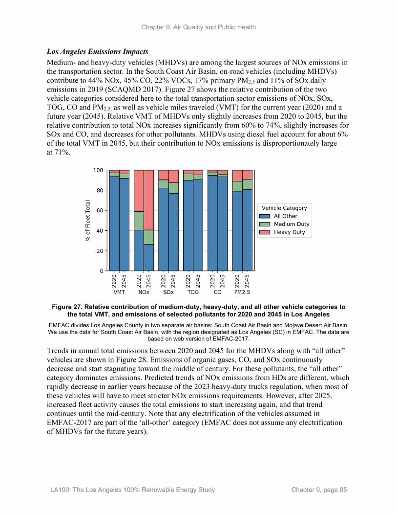
Chapter 9. Air Quality and Public Health
LA100: The Los Angeles 100% Renewable Energy Study Chapter 9, page 85
Los Angeles Emissions Impacts Medium- and heavy-duty vehicles (MHDVs) are among the largest sources of NOx emissions in the transportation sector. In the South Coast Air Basin, on-road vehicles (including MHDVs) contribute to 44% NOx, 45% CO, 22% VOCs, 17% primary PM2.5 and 11% of SOx daily emissions in 2019 (SCAQMD 2017). Figure 27 shows the relative contribution of the two vehicle categories considered here to the total transportation sector emissions of NOx, SOx, TOG, CO and PM2.5, as well as vehicle miles traveled (VMT) for the current year (2020) and a future year (2045). Relative VMT of MHDVs only slightly increases from 2020 to 2045, but the relative contribution to total NOx increases significantly from 60% to 74%, slightly increases for SOx and CO, and decreases for other pollutants. MHDVs using diesel fuel account for about 6% of the total VMT in 2045, but their contribution to NOx emissions is disproportionately large at 71%.
Figure 27. Relative contribution of medium-duty, heavy-duty, and all other vehicle categories to
the total VMT, and emissions of selected pollutants for 2020 and 2045 in Los Angeles EMFAC divides Los Angeles County in two separate air basins: South Coast Air Basin and Mojave Desert Air Basin. We use the data for South Coast Air Basin, with the region designated as Los Angeles (SC) in EMFAC. The data are
based on web version of EMFAC-2017.
Trends in annual total emissions between 2020 and 2045 for the MHDVs along with “all other” vehicles are shown in Figure 28. Emissions of organic gases, CO, and SOx continuously decrease and start stagnating toward the middle of century. For these pollutants, the “all other” category dominates emissions. Predicted trends of NOx emissions from HDs are different, which rapidly decrease in earlier years because of the 2023 heavy-duty trucks regulation, when most of these vehicles will have to meet stricter NOx emissions requirements. However, after 2025, increased fleet activity causes the total emissions to start increasing again, and that trend continues until the mid-century. Note that any electrification of the vehicles assumed in EMFAC-2017 are part of the ‘all-other’ category (EMFAC does not assume any electrification of MHDVs for the future years).

Chapter 9. Air Quality and Public Health
LA100: The Los Angeles 100% Renewable Energy Study Chapter 9, page 86
Figure 28. Projected changes in the emissions of various pollutants for medium-duty, heavy-duty,
and all other vehicle categories between 2020 and 2045 in Los Angeles Note that there is no electrification assumed for medium- and heavy-duty vehicles in EMFAC-2017.
Data source: EMFAC-2017
Health Impacts While heavy-duty vehicle emissions limits have become more stringent over the years, they still contribute substantially to ambient air pollution and related health burdens. Davidson et al. (2020) found that even with a substantial decrease (58%) in the O3 and PM2.5 attributable deaths caused by MHDV emissions between 2011 and 2025, the vehicle category still remains the second largest contributor to deaths behind light-duty vehicles, which is disproportionate to their VMT (see above discussion). Moreover, the in-use NOx emissions from diesel engines have been found to be higher than the certification limits, which further contributes to air quality impairment from this large emission source (Annenberg et al., 2017), and thus exacerbates the

Chapter 9. Air Quality and Public Health
LA100: The Los Angeles 100% Renewable Energy Study Chapter 9, page 87
health consequences. In-use emissions from heavy-duty trucks were found to be, on average, five times higher than the engine NOx certification limit during urban driving conditions (Posada, Badshah, and Rodriguez 2020). These urban driving condition emissions may cause disproportionate exposure to disadvantaged communities, many of which reside very close to highways where most urban driving occurs.
Emissions and Air Quality Impacts from MHDV Fleet Electrification: Literature Review Several recent studies have considered the air quality and health co-benefits from various electrification scenarios. Many of these studies are motivated by the State of California’s goal, through Assembly Bill 32, to reduce economy-wide greenhouse gas emissions to 40% by 2030, and 80% by mid-century compared to a 1990 reference level. These studies use current emission inventories and apply sector-specific emission control factors to estimate and create future emission inventories. Underlying assumptions for the scenarios, study regions, and expected benefits from relevant studies are summarized in Table 21(air quality benefits) and Table 22 (health benefits). These studies do not model the effects from electrification of MHDVs alone, but they assume a future where electrification of several other sectors occur to achieve the State’s GHG reduction goals. Therefore, the expected air quality and health benefits in Table 21 and Table 22 are not just due to medium- and heavy-duty fleet electrification, but a host of other (confounding) factors as well. It is therefore difficult without extensive re-analysis to quantitatively discern the contribution of MHDV electrification to total electrification results.
Most of these studies expect that emissions of PM2.5 and several gaseous precursors to PM2.5 will decrease, resulting in a decrease in atmospheric aerosol (PM) loading. Because exposure to PM2.5 dominates the health effects and their monetized value, most studies find significant public health benefits from future electrification scenarios. Impacts of various electrification scenarios are not as clear for O3 due to the nonlinearity in O3 formation chemistry and the regional photochemical regime that depends on the relative concentrations of NOx and VOCs. Some studies find that 8-hour maximum O3 concentration will decrease, while others report an increase.39 Most urban areas are generally NOx-saturated. In a NOx-saturated regime, a decrease in NOx concentration generally needs a simultaneous and large decrease in VOCs concentration to decrease O3, otherwise O3 may increase (see Figure 30 for an example) or if the focus is on NOx decrease, one can think this analogously to a “growing pains” phase before O3 starts decreasing (see Section 4.1.2.1 for a description of this). Nonetheless, some of these studies indicate that even with an O3 concentration increase, overall benefits for public health have a net positive signal because of a decrease in PM2.5 concentration.
39 A form of the 8-hour maximum O3 concentration is used to determine if an area meets the national ambient air quality standard (NAAQS). A summary of NAAQS for different pollutants is given in Appendix Table A-4.

Chapter 9. Air Quality and Public Health
LA100: The Los Angeles 100% Renewable Energy Study Chapter 9, page 88
Table 21. Summary of Literature that Estimates Emissions and Air Quality Benefits from Various Electrification Scenarios, including Medium- and Heavy-Duty Vehicle Electrification
For reference, U.S. EPA’s table on national ambient air quality standards for six criteria pollutants is provided in Table 23 (page 99) in the Supplemental Information at the end of this appendix.
Study
Focus Region and Modeling Year
Vehicle Classes Modeled Scenario Assumptions Emissions or Air Quality Benefits
Nopmongcol et al. (2017)
Continental United States, 2030
Light-duty, medium- and heavy-duty, and off-road equipment
Assumes 17% of light-duty, 8% of medium- and heavy-duty fleet VMT is all electric mode in 2030. Up to 80% of off-road equipment sales are electric. Only considers electrification of refuse trucks and single unit short-haul trucks.
O3 reduction attributable to electrification are <1 part per billion (ppb) for most of the United States, and 4–5 ppb for Los Angeles but the decrease is dominated by off-road equipment electrification. Annual change in PM2.5 is <0.5 µg/m3 for most of the United States, with largest reduction of 1.8 µg/m3 in Los Angeles
Sen et al. (2017)
United States Class 8 heavy-duty trucks
The study considers life cycle emissions. No air quality modeling was done.
Life cycle emissions of CO, NOx, and VOCs from battery electric heavy-duty trucks (Class 8 vehicles in Table 20) are considerably lower compared to conventional diesel trucks. Therefore, the expected lifetime impacts of battery electric heavy-duty trucks will far exceed their diesel counterparts and will improve the air quality.
Pan et al. (2019)
Greater Houston Area, 2040
All vehicle classes
Considers a base (2013 emissions), business as usual (BAU, no electric), moderate electrification (ME, 35% electric), aggressive electrification (AE, 70% electric) and complete turnover (35% electric, with all vehicles having improved emissions) scenarios.
Emissions increase by 50% in BAU, and decrease by 50%, 75%, and 95% in ME, AE and CT scenarios compared to 2013 base scenario. Maximum daily 8-hour average ozone increases by 1–3 ppb in ME, AE, and CT cases near highways because of a decrease in NOx emissions, and therefore reduced O3 titration by NOx. Overall, O3 concentrations decrease by 3–4 ppb in areas with high O3 in the base case. PM2.5 decreases in all electrification scenarios, with maximum increase close to highways (1–2 µg/m3) and decrease of less than 1 µg/m3 elsewhere.

Chapter 9. Air Quality and Public Health
LA100: The Los Angeles 100% Renewable Energy Study Chapter 9, page 89
Study
Focus Region and Modeling Year
Vehicle Classes Modeled Scenario Assumptions Emissions or Air Quality Benefits
ICF (2019) California, 2031 Medium- and heavy-duty vehicles
The study uses an ‘electricity’ scenario40 that attempts to meet the State’s NOx and GHG emission targets and an ‘electricity max’ scenario that intends to meet NOx emissions targets and exceeding GHG targets. The study did not model any air quality changes.
An 80% reduction in tailpipe NOx emissions from trucks and buses is required to meet the NAAQS for ozone in South Coast Air Basin in 2031 compared to 2019. None of the medium- or heavy-duty vehicle electrification scenarios help meet the State’s 2031 NOx emissions targets.
Marcus et al. (2019)
California and South Coast Air Basin. 2050 (also 2030)
Electrification for several sector is considered, including medium- and heavy-duty trucks
The future reference scenario for 2050 is based on the U.S. EPA and CARB emissions inventories. The 2050 electrification scenario builds on an ‘in-state biomass’ scenario with target to reduce GHG emissions by 80% relative to 1990 with additional mitigation strategies of increased reliance on industrial electrification, zero-emission vehicle (ZEV) trucks and renewables.
Emissions reductions in the South Coast Air Basin for the electrification scenario are 49% for NOx, 23% for primary PM2.5, 18% for VOCs, 14% for NH3, and 72% for CO. On-road vehicles in the electrification scenario account for 33% of NOx reductions, and 28% of VOCs reduction. Annual average PM2.5 decrease in large parts of LA County in the electrification scenario (by as much as 5 µg/m3 at some places), with the largest reduction coming from residential and commercial sector (>1 µg/m3), followed by on-road and industries (0.5–1.0 µg/m3), compared to the reference scenario. Overall, maximum daily 8-hour average O3 concentrations also decrease in the South Coast Air Basin in electrification scenario (by as much as 10–15 ppb) but increase in some parts of LA County (<3 ppb). On-road transportation leads to the reduction in O3 concentration by up to 3 ppb, and relatively smaller changes coming from other sectors. Only the “other anthropogenic” sector contributes to an
40 The ‘electricity’ scenario assumes a fleet of 100,000 electric medium-duty and heavy-duty vehicles in 2030 and more than 1.3 million of these vehicles in 2050. ‘Electricity Max’ scenario, defined as the upper limit of electrification potential, assumes 100% medium-duty and heavy-duty vehicle sales to be electric beginning in 2024, which equates to more than 800,000 electric MD and HD vehicles in 2030 and 2.2 million in 2050.

Chapter 9. Air Quality and Public Health
LA100: The Los Angeles 100% Renewable Energy Study Chapter 9, page 90
Study
Focus Region and Modeling Year
Vehicle Classes Modeled Scenario Assumptions Emissions or Air Quality Benefits
increase in O3 (3 ppb or less).41 However, the increase in O3 concentration occurs in areas where the reference case concentration is low (40–50 ppb). Therefore, this increase is unlikely to lead to any regulatory/compliance issues.
Forrest (2019) California, 2050. Two representative weeks in summer and winter are used for air quality modeling, with 11 days used for calculating average and peak change in pollutant concentration.
All vehicle classes, with specific focus on electrification of medium- and heavy-duty vehicles
A current policy reference scenario (aimed at 80% reduction in GHG emissions in 2050 compared to 1990) and several future expanded ZEV transportation scenarios are considered. Future scenarios are designed to reduce GHG emissions from each transportation sector (light-, medium-, heavy-duty, and buses) by 80% or beyond. These future scenarios consider a 40% heavy-duty ZEV (HD ZEV), 73% HD ZEV, High BEV and High H2 scenarios, with the last two scenarios very little GHG emissions from medium- and heavy-duty vehicles.
Peak summer ozone concentration (maximum daily 8-hour average) decreases by about 12 ppb in high BEV and high H2 scenarios, with 73% and 40% HD ZEV scenario reductions being 10.4 and 5.7 ppb, respectively. These high O3 concentration reductions mostly occur in South Coast Air Basin. 24-hour average PM2.5 concentrations decrease by approximately 4 µg/m3 for high BEV and high H2 scenarios, with a summertime average decrease of approximately 1µg/m3. Decrease in 24-hour average PM2.5 for winter is 3.5 µg/m3 and 1.5 µg/m3 for 73% and 40% HD ZEV scenarios, respectively. These high PM2.5 concentration reductions mostly occur in Central Valley, but South Coast Air Basin also benefits albeit by a smaller degree.
41 “Other anthropogenic” category includes sources in the inventory that are not categorized as transportation (on-road and off-road), residential and commercial, electricity generating units and industry. Some example sources included in ‘other anthropogenic’ are petroleum products storage, sea-borne transportation, etc.

Chapter 9. Air Quality and Public Health
LA100: The Los Angeles 100% Renewable Energy Study Chapter 9, page 91
Study
Focus Region and Modeling Year
Vehicle Classes Modeled Scenario Assumptions Emissions or Air Quality Benefits
EPRI (2020) South Coast Air Basin, California. Emissions for 2015–2050 at 5-year interval. Air quality modeling for 2030 and 2050
All vehicle classes, with emissions reductions from other electrifiable sources
Scenario designed to meet California’s economy-wide decarbonization targets of 40% and 80% in 2030 and 2050, respectively (relative to 1990). Scenario design also incorporate emission changes from California SB100.
NOx emissions in South Coast Air Basin decrease by 84% between 2011 and 2050. NOx emissions from heavy-duty vehicles decrease substantially in 2050 compared to the 2011 base year. Emissions of PM2.5 from heavy-duty vehicles also decrease. Design value42 of O3 decreases across the Los Angeles Basin. O3 design value at Santa Clarita monitor in LA County decreases by 30 ppb in 2050 and meets the 2015 NAAQS O3 standard of 70 ppb. Future year design value for PM2.5 decreases, and most monitors meet the NAAQS of 12 µg/m3. The decrease is largest for Los Angeles monitors. Most PM2.5 decrease is due to decrease in concentration of secondary inorganic aerosol, which occurs due to aggressive NOx and SO2 emission reduction in future years.
Wang et al. (2020)
California. 2050 Electrification across all vehicle classes (75% for LDV, 33% for bus, 10% for medium-duty trucks and 5% heavy-duty trucks)
A business as usual (BAU) scenario forms future baseline and assumed no additional climate policies are applied to BAU after 2010 (2050 GHG emissions in BAU are 156% relative to 2010). A net-zero scenario for 2050 assumes reduces reduced GHG emissions across all sectors.
In Southern California, NOx emissions decrease by about 50% in the net-zero scenario compared to BAU in 2050. Emissions of reactive organic gases, PM2.5, ammonia and SOx also decrease, but to a smaller extent then NOx. Population-weighted annual-average PM2.5 decrease in net-zero scenario are 8.4 µg/m3 in LA County and 7.8 µg/m3 in Orange County, and about 3–4 µg/m3 in other South Coast Air Basin counties. Maximum daily 8-hour average ozone increases by 2.5 ppb in LA County, 1.2 ppb in Orange County, and 0.5 ppb in San Bernardino County. There is a slight ozone reduction in Riverside County in net-zero scenario.
42 O3 design value is defined as the 4th highest maximum daily 8-hour average over three consecutive years.

Chapter 9. Air Quality and Public Health
LA100: The Los Angeles 100% Renewable Energy Study Chapter 9, page 92
Table 22. Summary of Literature that Estimates Health Benefits from Various Electrification Scenarios, including Medium- and Heavy-Duty Vehicle Electrification
Study Focus Region
Vehicle Classes Modeled
Scenario Assumptions Health Benefits
Pan et al. (2019)
Greater Houston Area, 2040
All Considers a base (2013 emissions), business as usual scenario (BAU, no electric), moderate electrification (ME, 35% electric), aggressive electrification (AE, 70% electric) and complete turnover (35% electric, with all vehicles having improved emissions) scenarios. Scenarios consider electrification of light- and heavy-duty vehicles. All heavy-duty electric vehicles are assumed to be battery electric, not hybrids.
Compared to the base year (2013), the BAU scenario causes 122 additional deaths due to increased emissions. ME, AE, and CT scenarios reduce premature deaths by 114, 188, and 246, respectively, in the greater Houston area, which includes eight counties.
Marcus et al. (2019)
California and South Coast Air Basin, 2050
Electrification for several sector is considered, including medium- and heavy-duty trucks
The future reference scenario for 2050 is based on the U.S. EPA and CARB emissions inventories. The 2050 electrification scenario builds on an ‘in-state biomass’ scenario with target to reduce GHG emissions by 80% relative to 1990 with additional mitigation strategies of increased reliance on industrial electrification, ZEV trucks, and renewables.
Electrification scenario results in approximately 6,400 avoided mortalities per year in South Coast Air Basin when no threshold for PM2.5 or O3 concentration health effects is used. This is equivalent to $56 billion dollars of monetary benefits. Benefits due to PM2.5 reduction are 97% of total benefits. Costs from O3 increase in parts of Los Angeles (see Table 21 entry for this study) are countered by large benefits from PM2.5 concentration decrease.
Wang et al. (2020)
California, 2050
Electrification across all vehicle classes (75% for LDV, 33% for bus, 10% for medium-duty trucks, and 5% heavy-duty trucks)
A business as usual (BAU) scenario forms future baseline and assumed no additional climate policies are applied to BAU after 2010 (2050 GHG emissions in BAU are 156% relative to 2010). A net-zero scenario for 2050 reduces GHG emissions across sectors.
Health benefits from PM2.5 reductions in net-zero scenario are significant. Approximately 9,300 mortalities are avoided in South Coast Air Basin counties area in year 2050, with 60% of these in LA County. Increases in O3 concentration in the net-zero scenario causes about 600 additional deaths in 2050, and 85% of these occur in LA County.
Chapter 9. Air Quality and Public Health
LA100: The Los Angeles 100% Renewable Energy Study Chapter 9, page 93
The air quality analysis presented in Chapter 9 considers emissions reductions of NOx, PM2.5, and other pollutants in the LA100-influenced sectors (power generation, transportation [light-duty vehicles and buses], buildings (commercial and residential), and the Ports of Los Angeles and Long Beach). Emission reductions in non-LA100-influenced sectors (e.g., MHDV) follow those included in the South Coast Air Quality emissions projection to 2031, at which point they are held constant to 2045 (see Section 3.1.5.2 in this chapter for more details). The SCAQMD 2031 project emissions inventory was developed for the 2016 air quality management plan and thus does not consider any emissions reductions from recent MHDV electrification-focused policies. For instance, Executive Order N-79-20 aims to achieve 100% MHDV fleet transition to zero-emission vehicles by 2045 and by 2035 for all drayage trucks.
The analysis of LA100 scenarios found that concentrations of PM2.5 decrease in all future scenarios, whereas ozone concentrations in most parts of the city increase (see Section 4.1.2.1 in this chapter). As explained in greater detail in the chapter, Los Angeles is in a NOx-saturated regime (i.e., NOx to VOC ratio is high). The atmospheric chemistry of ozone formation is complex and nonlinear, and it depends on relative emissions (and concentrations) of NOx and VOCs. In the scenarios modeled in LA100, NOx emissions decrease but the reduction is not sufficient to push the Los Angeles region outside of a NOx-saturated to a NOx-limited regime, wherein NOx emissions reductions result in ozone concentration reduction.
Focusing on the studies conducted in the South Coast Air Basin in Table 21, we see that one recent study investigated scenarios of electrification focused on the light-duty vehicle fleet (Wang et al., 2020), whereas others also considered higher electrification levels for MHDVs (Forrest et al., 2019; EPRI, 2020). Because MHDVs are a large source of NOx emissions in the South Coast Air Basin, electrification of LDVs is not enough to produce sufficient NOx emissions reduction to move past the “growing pains” described in the chapter (i.e., to transition from NOx-saturated to NOx-limited regime). Focusing on LDV electrification as modeled in the prior studies leads to ozone concentration increases, as seen in the LA100 scenario results and also found by Wang et al. (2020). When MHDV electrification is added to NOx emissions reductions in other sectors (including LDV electrification), ozone concentration is found to decrease (Forrest et al., 2019; EPRI, 2020). Thus, NOx emissions reductions from MHDV electrification with high electrification in LDV and other end-use sectors (such as off-road equipment) appears to move LA past the “growing pains” zone to where ozone concentration could be reduced in the basin.
Other Considerations for Air Quality for MHDV: Increasing Importance of Brake Wear and Tire Wear Emissions Predictions based on emission models (CARB’s EMFAC and U.S. EPA’s Motor Vehicle Emission Simulator (MOVES) models, although MOVES emission factors are lower for brake and tire wear) suggest that, with increasingly stringent exhaust emission standards, traffic-related emissions of particulate matter will become proportionally dominated by non-exhaust sources, within the context of an overall effect of reducing PM emissions from vehicles (Reid et al. 2016). Some recent near-road air quality analysis studies show that non-exhaust emissions dominate total emissions, with 60% of the total modeled PM2.5 emissions (although road-dust dominates the total emissions within non-exhaust emissions, see, e.g., Craig et al. 2020). However, this relative contribution of tire and brake wear will likely increase in the future. As an example, this is shown in Figure 29 for Los Angeles for two different years (2020 and 2045), indicating that

Chapter 9. Air Quality and Public Health
LA100: The Los Angeles 100% Renewable Energy Study Chapter 9, page 94
exhaust emissions are expected to decrease significantly, and relative contribution of non-exhaust emissions increase.
Figure 29. Contribution of various emission processes to total PM2.5 emissions in 2020 and 2045
for MHDVs Data Source: California Air Resources Board’s EMFAC model (EMFAC 2017)
Studies have shown that non-exhaust particulate matter emissions, including tire wear, brake wear, and road wear, depend on vehicle size and are positively correlated with vehicle weight (Simons 2016; Timmers and Achten 2016). These vehicle characteristics for different vehicle classes are also accounted for in emissions models such as MOVES and EMFAC, (i.e., non-exhaust particulate matter emissions factors differ among passenger cars, light-duty trucks, and heavy-duty trucks. However, non-exhaust PM emission factors for EVs will likely be different from their conventional counterparts, for instance because EVs are generally heavier due to weight of batteries (Requia et al. 2018). However, there are some areas where further research is needed to improve understanding of these non-exhaust emissions. These areas of research include, for example, impact of regenerative braking on emissions, driving conditions, and driving behavior. Understanding their impact on particulate emissions is important to accurately model emissions with changing fleet characteristics. More research is also needed to assess toxicity potential of brake and tire wear particles so that emissions reduction from these sources could be appropriately strategized (Gerlofs-Nijland et al. 2019; Kreider, Unice, and Panko 2019).
Fleet Turnover and Need for Prioritizing Electrification of Super Emitters Fleet turnover refers to changes in fleet characteristics. As vehicles age, some are phased out whereas others continue to operate. Some of these medium- and heavy-duty vehicles emit some pollutants (mostly PM2.5, NOx and NH3) at much higher levels than certifications and the rest of the fleet; these vehicles are called super emitters. The extremely high emissions from super emitters are usually caused by poor engine maintenance, non-compliance with regulations, or a failure of the emissions control systems. Some recent studies have highlighted the role of super emitters in impairing air quality. Pan et al. (2019) used a photochemical model to study the potential benefits of phasing out super-emitter MHDVs, which decreased emissions of primary PM2.5 greater than the emissions reductions associated with a stringent emission control scenario (one that is applied evenly across all vehicles of a given class). Pen and colleagues found that

Chapter 9. Air Quality and Public Health
LA100: The Los Angeles 100% Renewable Energy Study Chapter 9, page 95
such a scenario improved air quality across the country, saving several hundred lives, with the largest number of avoided premature deaths occurring in Los Angeles (Pan et al. 2019). Monetized benefits from the super-emitter phasing-out scenario were several billion dollars. In the South Coast Air Basin, automobiles can be a significant source of NH3 emissions which, under favorable thermodynamic conditions, can form particles of ammonium nitrate (NH4NO3) and which constitute a large fraction of PM2.5 mass in the basin (Nowak et al. 2012). Automobile NH3 emissions result from use of selective catalytic reduction (SCR), a technology to control vehicular NOx emissions. A recent study found that NH3 emissions are disproportionately high from heavy-duty trucks with SCR (10% of heavy-duty trucks contribute to 95% of total on-road vehicle NH3 emissions) (Preble et al. 2018). MHDV electrification targeted toward super emitters is likely to reduce exhaust emissions of PM2.5, NOx, and NH3 that contribute to formation of PM2.5 and O3 and thus yield more health benefits.
A.6 Environmental Justice Implications
Communities Near Roads Recent modeling and monitoring analysis have shown that near-road concentration of PM2.5 could be higher than the nearby non-near road or background monitors by about 1 µg/m3 (DeWinter et al. 2018; Craig et al. 2020; Gantt, Owen, and Watkins 2021). Some recent studies have shown that electrification will benefit environmentally disadvantaged communities. For example, Wang et al. (2020)43 found that an electrified future with net-zero GHG emissions has air quality and health co-benefits that are disproportionately higher in the disadvantaged communities (35% of the avoided deaths in 2050 are from 25% of the state’s disadvantaged community population). Approximately 5,000 of the estimated total of 14,000 avoided deaths in California are in the state’s disadvantaged communities, with a significantly large fraction of these avoided mortalities in the Los Angeles region. Similarly, a study conducted by California Energy Commission (CEC) (Marcus et al. 2019)43 also found that health benefits from electrification were slightly higher in disadvantaged communities. Per the CEC study, 28% of the total air quality benefits occur in disadvantaged communities, representing a monetized value of $31 billion dollars. However, it will still be important to assess impacts on communities living near roadways given that primary PM2.5 has large concentration gradients and is thus likely to have the largest impact close to the source—so the previously mentioned role of non-exhaust emissions becomes even more important. This becomes important because of the concerns around increased exposure due to proposed land use and transportation plans in California, which will likely result in larger populations close to the roadways.44
Communities Near Ports of Los Angeles and Long Beach Because we modeled the electrification of heavy-duty trucks at the ports of Los Angeles and Long Beach as part of the air quality modeling component of the LA100 study, the benefits on air quality and thus for surrounding disadvantaged communities are available as part of the final report. Because of the nature of how air pollutants form, it is not possible to quantitatively
43 See Table 21 and Table 23 for details on the air quality and health benefits from electrification scenarios modeled in these studies. 44 “Brake and Tire Wear Emissions: Vehicle Non-Exhaust Particulate Matter Sources, CARB, https://ww2.arb.ca.gov/resources/documents/brake-tire-wear-emissions#_ftn1.

Chapter 9. Air Quality and Public Health
LA100: The Los Angeles 100% Renewable Energy Study Chapter 9, page 96
discern specific sources contribution to changes in air quality and health, but the role of reductions of emissions at the Ports is assessed in our overall analysis.
A.7 GHG Emissions Benefits GHG impacts associated with the electrification of MHDVs would be expected to follow a trend similar to that quantified for the light-duty vehicles and buses, as described in Chapter 8. Specifically, as an increasing share of the vehicle fleet becomes electric, a decreasing amount of GHG emissions will be associated with the combustion of fossil-derived transportation fuels (e.g., gasoline, diesel, compressed natural gas (CNG), and propane) in the fleet. One slight difference between the quantified impacts seen in the light-duty vehicle and bus GHG impacts and what would likely be seen in MHDV electrification scenarios is that the proportional reduction in GHG emissions associated with an increase in fleet electrification might be slightly higher than the impact from a similar electrification increase in the LDV/bus fleets. This is surmised due to the higher prevalence of diesel-fueled vehicles in the MHDV fleet compared to the fuels used in the other fleets and knowing that diesel has a higher GHG intensity than gasoline or other fossil fuels. This is especially likely to be the case when comparing to emissions reductions from electrification of the bus fleets, as a majority of both urban and school buses in LA have already transitioned from diesel to be fueled by CNG or propane, both of which entail lower life cycle GHG emissions factors than diesel fuel.
A.8 References Anenberg, Susan C., Joshua Miller, Daven K. Henze, Ray Minjares, and Pattanun Achakulwisut. 2019. “The Global Burden of Transportation Tailpipe Emissions on Air Pollution-Related Mortality in 2010 and 2015.” Environmental Research Letters 14 (9): 094012. https://doi.org/10.1088/1748-9326/ab35fc.
Craig, Kenneth J., Lynn M. Baringer, Shih-Ying Chang, Michael C. McCarthy, Song Bai, Annie F. Seagram, Vikram Ravi, Karin Landsberg, and Douglas S. Eisinger. 2020. “Modeled and Measured Near-Road PM2.5 Concentrations: Indianapolis and Providence Cases.” Atmospheric Environment 240 (November): 117775. https://doi.org/10.1016/j.atmosenv.2020.117775.
Davidson, Kenneth, Neal Fann, Margaret Zawacki, Charles Fulcher, and Kirk R. Baker. 2020. “The Recent and Future Health Burden of the U.S. Mobile Sector Apportioned by Source.” Environmental Research Letters 13. https://doi.org/10.1088/1748-9326/ab83a8.
DeWinter, Jennifer L., Steven G. Brown, Annie F. Seagram, Karin Landsberg, and Douglas S. Eisinger. 2018. “A National-Scale Review of Air Pollutant Concentrations Measured in the U.S. near-Road Monitoring Network during 2014 and 2015.” Atmospheric Environment 183 (June): 94–105. https://doi.org/10.1016/j.atmosenv.2018.04.003.
EPRI (Electric Power Research Institute). 2020. Efficient Electrification in California: Assessment of Energy System and Air Quality Impacts. Technical Report 000000003002019494. Electric Power Research Institute. https://www.epri.com/research/products/3002019494.
Fann, Neal, Charles M. Fulcher, and Kirk Baker. 2013. “The Recent and Future Health Burden of Air Pollution Apportioned Across U.S. Sectors.” Environmental Science & Technology 47 (8): 3580–3589. https://doi.org/10.1021/es304831q.

Chapter 9. Air Quality and Public Health
LA100: The Los Angeles 100% Renewable Energy Study Chapter 9, page 97
Gantt, Brett, R. Chris Owen, and Nealson Watkins. 2021. “Characterizing Nitrogen Oxides and Fine Particulate Matter near Major Highways in the United States Using the National Near-Road Monitoring Network.” Environmental Science & Technology 55 (5): 2831–2838. https://doi.org/10.1021/acs.est.0c05851.
Gerlofs-Nijland, M. E., B. G. H. Bokkers, H. Sachse, J. J. E. Reijnders, M. Gustafsson, A. J. F. Boere, P. F. H. Fokkens, D. L. A. C. Leseman, K. Augsburg, and F. R. Cassee. 2019. “Inhalation Toxicity Profiles of Particulate Matter: A Comparison between Brake Wear with Other Sources of Emission.” Inhalation Toxicology 31 (3): 89–98. https://doi.org/10.1080/08958378.2019.1606365.
Hill, Bruce. 2005. An Analysis of Diesel Air Pollution and Public Health in America. Clean Air Task Force. http://www.catf.us/wp-content/uploads/2019/02/CATF_WhitePaper_Diesel_Air_Pollution_Analysis.pdf.
ICF. 2019. Comparison of Medium and Heavy Duty Technologies in California. https://caletc.com/wp-content/uploads/2019/12/ICF-Truck-Report_Final_December-2019.pdf.
Kreider, Marisa L., Ken M. Unice, and Julie M. Panko. 2019. “Human Health Risk Assessment of Tire and Road Wear Particles (TRWP) in Air.” Human and Ecological Risk Assessment: An International Journal 0 (0): 1–19. https://doi.org/10.1080/10807039.2019.1674633.
Marcus, Alexander, Ana Alvarez-Gomez, Daniel Bowermaster, John Grant, Brandon Johnson, Eladio Knipping, Sreenidhi Krishnamoorthy, et al. 2019. Air Quality Implications of an Energy Scenario for California Using High Levels of Electrification. CEC-500-2019-049. California Energy Commission. https://ww2.energy.ca.gov/2019publications/CEC-500-2019-049/CEC-500-2019-049.pdf.
Nopmongcol, Uarporn, John Grant, Eladio Knipping, Mark Alexander, Rob Schurhoff, David Young, Jaegun Jung, Tejas Shah, and Greg Yarwood. 2017. “Air Quality Impacts of Electrifying Vehicles and Equipment Across the United States.” Environmental Science & Technology 51 (5): 2830–2837. https://doi.org/10.1021/acs.est.6b04868.
Nowak, J. B., J. A. Neuman, R. Bahreini, A. M. Middlebrook, J. S. Holloway, S. A. McKeen, D. D. Parrish, T. B. Ryerson, and M. Trainer. 2012. “Ammonia Sources in the California South Coast Air Basin and Their Impact on Ammonium Nitrate Formation.” Geophysical Research Letters 39 (7). https://doi.org/10.1029/2012GL051197.
Pan, Shuai, Anirban Roy, Yunsoo Choi, Ebrahim Eslami, Stephanie Thomas, Xiangyu Jiang, and H. Oliver Gao. 2019. “Potential Impacts of Electric Vehicles on Air Quality and Health Endpoints in the Greater Houston Area in 2040.” Atmospheric Environment 207 (June): 38–51. https://doi.org/10.1016/j.atmosenv.2019.03.022.
Pan, Shuai, Anirban Roy, Yunsoo Choi, ShiQuan Sun, and H. Oliver Gao. 2019. “The Air Quality and Health Impacts of Projected Long-Haul Truck and Rail Freight Transportation in the United States in 2050.” Environment International 130 (September): 104922. https://doi.org/10.1016/j.envint.2019.104922.

Chapter 9. Air Quality and Public Health
LA100: The Los Angeles 100% Renewable Energy Study Chapter 9, page 98
Posada, Francisco, Huzeifa Badshah, and Felipe Rodriguez. 2020. In-Use NOx Emissions and Compliance Evaluation for Modern Heavy-Duty Vehicles in Europe and The United States. The International Council on Clean Transportation. https://theicct.org/sites/default/files/publications/In-use-NOx%20emissions-May2020.pdf.
Preble, Chelsea V., Troy E. Cados, Robert A. Harley, and Thomas W. Kirchstetter. 2018. “In-Use Performance and Durability of Particle Filters on Heavy-Duty Diesel Trucks.” Environmental Science & Technology 52 (20): 11913–11921. https://doi.org/10.1021/acs.est.8b02977.
Reid, Stephen, Song Bai, Yuan Du, Kenneth Craig, Garnet Erdakos, Lynn Baringer, Douglas Eisinger, Michael McCarthy, and Karin Landsberg. 2016. “Emissions Modeling with MOVES and EMFAC to Assess the Potential for a Transportation Project to Create Particulate Matter Hot Spots.” Transportation Research Record 2570 (1): 12–20. https://doi.org/10.3141/2570-02.
Requia, Weeberb J., Moataz Mohamed, Christopher D. Higgins, Altaf Arain, and Mark Ferguson. 2018. “How Clean Are Electric Vehicles? Evidence-Based Review of the Effects of Electric Mobility on Air Pollutants, Greenhouse Gas Emissions and Human Health.” Atmospheric Environment 185 (July): 64–77. https://doi.org/10.1016/j.atmosenv.2018.04.040.
SCAQMD. 2017. 2016 Air Quality Management Plan: Appendix III Base and Future Year Emission Inventory. South Coast Air Quality Management District. https://www.aqmd.gov/docs/default-source/clean-air-plans/air-quality-management-plans/2016-air-quality-management-plan/final-2016-aqmp/appendix-iii.pdf?sfvrsn=6.
Sen, Burak, Tolga Ercan, and Omer Tatari. 2017. “Does a Battery-Electric Truck Make a Difference?–Life Cycle Emissions, Costs, and Externality Analysis of Alternative Fuel-Powered Class 8 Heavy-Duty Trucks in the United States.” Journal of Cleaner Production 141 (January): 110–21. https://doi.org/10.1016/j.jclepro.2016.09.046.
Simons, Andrew. 2016. “Road Transport: New Life Cycle Inventories for Fossil-Fuelled Passenger Cars and Non-Exhaust Emissions in Ecoinvent V3.” The International Journal of Life Cycle Assessment 21 (9): 1299–1313. https://doi.org/10.1007/s11367-013-0642-9.
Timmers, Victor R. J. H., and Peter A. J. Achten. 2016. “Non-Exhaust PM Emissions from Electric Vehicles.” Atmospheric Environment 134 (June): 10–17. https://doi.org/10.1016/j.atmosenv.2016.03.017.
U.S. EPA (U.S. Environmental Protection Agency). 2002. Health Assessment Document For Diesel Engine Exhaust. EPA/600/8-90/057F. https://nepis.epa.gov/Exe/ZyPDF.cgi/300055PV.PDF?Dockey=300055PV.PDF.
Wang, Tianyang, Zhe Jiang, Bin Zhao, Yu Gu, Kuo-Nan Liou, Nesamani Kalandiyur, Da Zhang, and Yifang Zhu. 2020. “Health Co-Benefits of Achieving Sustainable Net-Zero Greenhouse Gas Emissions in California.” Nature Sustainability, May 1–9. https://doi.org/10.1038/s41893-020-0520-y.
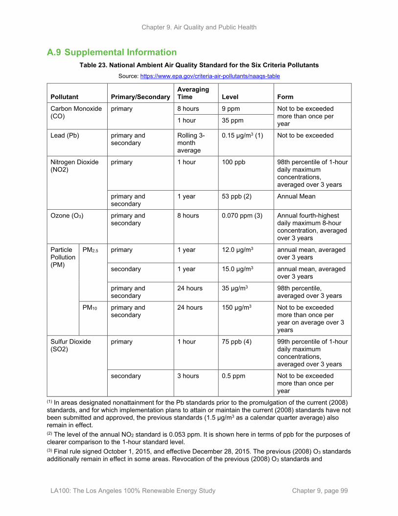
Chapter 9. Air Quality and Public Health
LA100: The Los Angeles 100% Renewable Energy Study Chapter 9, page 99
A.9 Supplemental Information Table 23. National Ambient Air Quality Standard for the Six Criteria Pollutants
Source: https://www.epa.gov/criteria-air-pollutants/naaqs-table
Pollutant Primary/Secondary Averaging Time Level Form
Carbon Monoxide (CO)
primary 8 hours 9 ppm Not to be exceeded more than once per year 1 hour 35 ppm
Lead (Pb) primary and secondary
Rolling 3-month average
0.15 μg/m3 (1) Not to be exceeded
Nitrogen Dioxide (NO2)
primary 1 hour 100 ppb 98th percentile of 1-hour daily maximum concentrations, averaged over 3 years
primary and secondary
1 year 53 ppb (2) Annual Mean
Ozone (O3) primary and secondary
8 hours 0.070 ppm (3) Annual fourth-highest daily maximum 8-hour concentration, averaged over 3 years
Particle Pollution (PM)
PM2.5 primary 1 year 12.0 μg/m3 annual mean, averaged over 3 years
secondary 1 year 15.0 μg/m3 annual mean, averaged over 3 years
primary and secondary
24 hours 35 μg/m3 98th percentile, averaged over 3 years
PM10 primary and secondary
24 hours 150 μg/m3 Not to be exceeded more than once per year on average over 3 years
Sulfur Dioxide (SO2)
primary 1 hour 75 ppb (4) 99th percentile of 1-hour daily maximum concentrations, averaged over 3 years
secondary 3 hours 0.5 ppm Not to be exceeded more than once per year
(1) In areas designated nonattainment for the Pb standards prior to the promulgation of the current (2008) standards, and for which implementation plans to attain or maintain the current (2008) standards have not been submitted and approved, the previous standards (1.5 µg/m3 as a calendar quarter average) also remain in effect. (2) The level of the annual NO2 standard is 0.053 ppm. It is shown here in terms of ppb for the purposes of clearer comparison to the 1-hour standard level. (3) Final rule signed October 1, 2015, and effective December 28, 2015. The previous (2008) O3 standards additionally remain in effect in some areas. Revocation of the previous (2008) O3 standards and
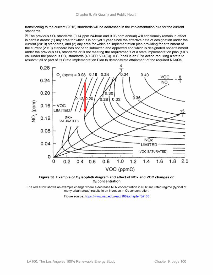
Chapter 9. Air Quality and Public Health
LA100: The Los Angeles 100% Renewable Energy Study Chapter 9, page 100
transitioning to the current (2015) standards will be addressed in the implementation rule for the current standards. (4) The previous SO2 standards (0.14 ppm 24-hour and 0.03 ppm annual) will additionally remain in effect in certain areas: (1) any area for which it is not yet 1 year since the effective date of designation under the current (2010) standards, and (2) any area for which an implementation plan providing for attainment of the current (2010) standard has not been submitted and approved and which is designated nonattainment under the previous SO2 standards or is not meeting the requirements of a state implementation plan (SIP) call under the previous SO2 standards (40 CFR 50.4(3)). A SIP call is an EPA action requiring a state to resubmit all or part of its State Implementation Plan to demonstrate attainment of the required NAAQS.
Figure 30. Example of O3 isopleth diagram and effect of NOx and VOC changes on
O3 concentration The red arrow shows an example change where a decrease NOx concentration in NOx saturated regime (typical of
many urban areas) results in an increase in O3 concentration.
Figure source: https://www.nap.edu/read/1889/chapter/8#165
(VOC SATURATED)
(NOx SATURATED)

Chapter 9. Air Quality and Public Health
LA100: The Los Angeles 100% Renewable Energy Study Chapter 9, page 101
Appendix B. Additional Information on Methods and Results for Air Quality Analysis B.1 Additional Information on Model Configuration The physics schemes used in our model configuration are as follows: the Lin cloud microphysics scheme (Lin et al., 1983), the RRTM longwave radiation scheme (Mlawer et al., 1997), the Goddard shortwave radiation scheme (Chou and Suarez, 1999), the MM5 similarity surface layer scheme (Dyer and Hicks, 1970; Paulson, 1970), the unified Noah land surface model (Chen et al., 2001), the YSU boundary layer scheme (Hong et al., 2006), the Grell 3D ensemble cumulus cloud scheme (Grell and Dévényi, 2002), and the urban canopy model (UCM) (Kusaka et al., 2001; Chen et al., 2011; Yang et al., 2015). The chemistry schemes we adopt in this study include the TUV photolysis scheme (Madronich, 1987), RACM-ESRL gas phase chemistry (Stockwell et al., 1997; Kim et al., 2009), and the MADE/VBS aerosol scheme (Ackermann et al., 1998; Ahmadov et al., 2012).
The meteorological initial and boundary conditions used in both the 2012 baseline and the four future scenarios are from the Global Forecast System Analysis Data (GFS-ANL) Historical Archive for July (National Centers for Environmental Prediction, 2007), and the North American Regional Reanalysis (NARR) data set (Mesinger et al., 2006) for all other three months to achieve better model evaluation with historical observations. The chemistry initial and boundary conditions for all scenarios are from the Model for Ozone and Related chemical Tracers, version 4 (MOZART-4) (Emmons et al., 2010). We use all available gas-phase species in MOZART-4. Note that we use the same meteorological and chemical initial and boundary conditions for both the 2012 baseline and future scenarios to avoid introducing additional sources of variability (i.e., the potential influence of changes in global chemistry and climate change on ozone mixing ratio and PM2.5 concentrations in Los Angeles). We aim to single out changes in air quality due to potential future reductions in urban emissions.
Following our previous publications (Vahmani and Ban-Weiss, 2016) and (Li et al., 2019), we modified WRF-Chem v3.7 to include a realistic representation of land surface properties and processes within urban areas. Accurately characterizing the land surface is critical for attaining good model performance of urban meteorology and air quality. For all simulations we use the 33-category National Land Cover Database (NLCD) for determining land cover type for all model domains (Fry et al., 2011), the National Urban Database and Access Portal Tool (NUDAPT) for building morphology where available for the innermost domain (Ching et al., 2009), and MODIS-retrieved albedo, green vegetation fraction (GVF), and leaf area index (LAI) for the innermost domain. Data are available for download at http://earthexplorer.usgs.gov. In addition, we also incorporate a Los Angeles Basin-specific irrigation scheme (Vahmani and Hogue, 2014).
For the emission inventory used for the innermost domain, note that there are differences in grid settings and speciation schemes between the SCAQMD emission inventory and our model set-up. Thus, we re-gridded the inventory and converted from SAPRC speciation to RADM2 speciation (Stockwell et al., 1997). Details on species mapping from SAPRC to RADM2 can be found in (Li et al., 2019).

Chapter 9. Air Quality and Public Health
LA100: The Los Angeles 100% Renewable Energy Study Chapter 9, page 102
B.2 Model Evaluation of Simulated O3 and PM2.5 Concentrations with Historical Observations We evaluated simulated daily maximum 8-hour O3 concentrations in July and daily averaged PM2.5 concentrations in all four months in Baseline (2012) against historical observations. Note that we only include evaluation of July O3 concentrations here because we are only presenting July O3 concentrations as representative of O3 season in result section. We obtain 8-hour O3 concentrations from Air Quality System (AQS, data available at https://www.epa.gov/aqs) for the innermost model domain and transfer the data to daily maximum 8-hour O3 concentrations. Daily averaged PM2.5 concentrations for the innermost domain are gathered from AQS and the Interagency Monitoring of Protected Visual Environments (IMPROVE, data available at http://views.cira.colostate.edu/fed/SiteBrowser/Default.aspx). Table 24 shows the statistics of model evaluation against those observations. Mean bias (MB), normalized mean bias (NMB), mean error (ME), normalized mean error (NME), mean fractional bias (MFB) and mean fractional error (MFE) are listed in the table. Evaluation benchmarks for some of the statistical suggested by U.S. Environmental Protection Agency (EPA) and literatures are listed in Table 25.
Table 24. Statistics of Model Evaluationa
Species Month Obs Mod MB NMB ME NME MFB MFE
Daily averaged PM2.5
Jan. 11.1 12.2 1.1 10% 6.0 54% 18% 56%
Daily averaged PM2.5
Apr. 9.0 8.0 -1.0 -12% 3.5 39% -3% 44%
Daily averaged PM2.5
July 10.3 10.3 0.0 0% 3.5 34% 1% 32%
Daily averaged PM2.5
Oct. 9.3 9.8 0.5 6% 3.5 37% 7% 39%
Daily maximum 8-hour O3
July 59.4 50.9 -8.5 -14% 11.7 20% -15% 22%
a Obs is the spatially and temporally averaged observed concentrations across all observation sites. Mol stands for the spatially and temporally averaged simulated concentrations at those observation sites. Obs, Mol, MB, ME are in unit of µg/m3 for daily averaged PM2.5 concentrations. Those statistics for daily maximum 8-hour O3 are in unit of ppb.

Chapter 9. Air Quality and Public Health
LA100: The Los Angeles 100% Renewable Energy Study Chapter 9, page 103
Table 25. Recommended Benchmarks of Statistical for Model Evaluation of Air Pollutant
Species NMB NME MFB MFE Reference
Daily PM2.5
< ±30% < 50% < ±30% < ±50% NMB and NME: https://www3.epa.gov/ttn/scram/guidance/guide/O3-PM-RH-Modeling_Guidance-2018.pdf MFB and MFE: (Boylan and Russell, 2006)
Daily maximum 8-hour O3
< ±15% < 25% / / https://www3.epa.gov/ttn/scram/guidance/guide/O3-PM-RH-Modeling_Guidance-2018.pdf
B.3 Explanation on Raw Emissions Used for Emission Projections The choice of whether to use SCAQMD 2012 raw emission (residential building and commercial building) or SCAQMD 2031 projection (other sectors except power plants) is dependent on whether scaling factors for activity from 2031 to 2045 are available or not. The factors to project fuel consumption in residential and commercial buildings from 2031 to 2045 are not available because dsgrid does not output 2031 result, so we project emission first from 2012 to 2020 using scaling factor for activities from SCAQMD, and then from 2020 to 2045 using dsgrid outputs.
B.4 Site-Specific Emission Factors for LADWP-Owned Power Plants Applied to Emission Projection in the SB100 and Early & No Biofuels Scenarios Emission factors are in the unit of lbs/MMBTU. CT under Category is natural gas combustion turbine power plant, CC is natural gas combined cycle power plant, H2 is hydrogen storage combustion power plant (built in RPM model). CT and CC are allowed in SB100, and only H2 is allowed in Early & No Biofuels. Values in black are based on LADWP emission reporting system (year 2019), values in red are set to regulatory limit, values in purple are assumed to be zero.
Table 26. Emission Factors Used in the SB100 Scenario
Power Plant Category CO NOx SOx VOC PM NH3
Harbor CT 0.0056 0.0092 0.00025 0.0022 0.0030 0.0069
Haynes CT 0.0042 0.0085 0.00027 0.00070 0.0014 0.0026
Scattergood CC 0.0022 0.0058 0.00028 0.00066 0.0016 0.0014
Valley CC 0.00066 0.0074 0.00040 0.00070 0.00071 0.0028
Valley CT 0.0037 0.0092 0.00039 0.00092 0.00023 0.0035

Chapter 9. Air Quality and Public Health
LA100: The Los Angeles 100% Renewable Energy Study Chapter 9, page 104
Table 27. Emission Factors Used in the Early & No Biofuels Scenario
Power Plant Category CO NOx SOx VOC PM NH3
Harbor H2 0 0.0063 0 0 0 0.0047
Haynes H2 0 0.0063 0 0 0 0.0047
Scattergood H2 0 0.0063 0 0 0 0.0047
Victorville H2 0 0.0063 0 0 0 0.0047
B.5 Scaling Factors Used for Projection of Transportation Emission Sources These data are available on request from Professor George Ban-Weiss at the University of Southern California.
B.6 Scaling Factors Used for Projection of Emissions from Commercial and Residential Buildings Table 28. Scaling Factors of Fuel Consumption in Commercial Buildings from 2020 to 2045 under
Moderate and High Electrification Assumptions
Month Moderate High
1 125.8% 3.5%
2 126.7% 3.5%
3 125.3% 3.7%
4 135.4% 2.6%
5 142.3% 2.2%
6 142.9% 2.2%
7 142.5% 2.2%
8 144.1% 2.2%
9 145.5% 2.1%
10 141.9% 2.2%
11 134.0% 2.6%
12 113.2% 5.1%

Chapter 9. Air Quality and Public Health
LA100: The Los Angeles 100% Renewable Energy Study Chapter 9, page 105
Table 29. Scaling Factors of Fuel Consumption in Residential Buildings from 2020 to 2045 under Moderate and High Electrification Assumptions
Month Moderate High
1 77.6% 13.4%
2 77.5% 13.5%
3 77.7% 13.6%
4 74.6% 13.0%
5 75.0% 13.7%
6 77.3% 16.9%
7 77.7% 17.4%
8 78.7% 17.8%
9 79.1% 17.3%
10 77.2% 13.8%
11 75.2% 12.5%
12 78.0% 13.9%
B.7 Emission Inventories for NOx and PM2.5 in Los Angeles from all Anthropogenic Sources for the Selected LA100 Scenarios
Figure 31. Annually averaged daily NOx emissions from all anthropogenic sources in Los Angeles
for all selected scenarios

Chapter 9. Air Quality and Public Health
LA100: The Los Angeles 100% Renewable Energy Study Chapter 9, page 106
Emissions for the selected future scenarios (SB100 – Moderate, SB100 – High, Early & No Biofuels – Moderate and Early & No Biofuels – High) are projected to year 2045. Note that ‘LADWP-owned Power Plants’ include those located in the South Coast Air Basin. Some representative contributors to “Other” include off-road equipment, trains, Regional Clean Air Incentives Market (RECLAIM) and aircraft for all scenarios.45
Figure 32. Annually averaged daily PM2.5 emissions from all anthropogenic sources in Los
Angeles for all selected scenarios Emissions for the selected future scenarios (SB100 – Moderate, SB100 – High, Early & No Biofuels – Moderate and Early & No Biofuels – High) are projected to year 2045. Note that ‘LADWP-owned Power Plants’ include those located in the South Coast Air Basin. Some representative contributors to “Other” include cooking, road dust, off-road equipment and mineral processes for Baseline (2012), and cooking, road dust, wood and paper, and mineral processes for the four future scenarios.46
45 Based on appendix A of Appendix III: Base and Future Year Emission Inventory in Final 2016 Air Quality Management Plan (http://www.aqmd.gov/docs/default-source/clean-air-plans/air-quality-management-plans/2016-air-quality-management-plan/final-2016-aqmp/appendix-iii.pdf). 46 Based on Appendix A of Appendix III: Base and Future Year Emission Inventory in Final 2016 Air Quality Management Plan (SCAQMD, 2017), http://www.aqmd.gov/docs/default-source/clean-air-plans/air-quality-management-plans/2016-air-quality-management-plan/final-2016-aqmp/appendix-iii.pdf.

Chapter 9. Air Quality and Public Health
LA100: The Los Angeles 100% Renewable Energy Study Chapter 9, page 107
B.8 Emission Inventories for CO, SOx, VOC, and NH3 from LA100-Influenced Sectors in Los Angeles for the Selected LA100 Scenarios
Figure 33. Annually averaged daily CO emissions from LA100-influenced sources in Los Angeles
for all selected scenarios Emissions for the selected future scenarios (SB100 – Moderate, SB100 – High, Early & No Biofuels – Moderate and Early & No Biofuels – High) are projected to year 2045. The percentage above each bar represents the fractional contribution of emissions from LA100-affected sources to all anthropogenic sources. Note that ‘LADWP-owned Power Plants’ include those located in the South Coast Air Basin.

Chapter 9. Air Quality and Public Health
LA100: The Los Angeles 100% Renewable Energy Study Chapter 9, page 108
Table 30. Annually Averaged Daily CO Emissions (metric tons/day) from LA100-Influenced Sources in Los Angeles and Citywide Total Emissions for all Selected Scenarios
Percentages in the parentheses show the percentage contribution of emissions from an LA100-influenced source to citywide total emissions in a scenario. Future scenarios are projected to year 2045.
Panel (a)
LADWP-Owned Power Plants
The Ports of LA and LB
Residential Buildings
Commercial Buildings LDVs Buses
Baseline (2012) 1.9 (0.3%)
3.4 (0.5%)
3.4 (0.5%)
0.32 (0.05%)
310 (46%)
8.8 (1%)
SB100 – Moderate 0.06
(0.02%) 0.30
(0.1%) 2.0
(0.6%) 0.39
(0.1%) 33
(11%) 0
SB100 – High 0.05 (0.02%)
0.18 (0.06%)
0.37 (0.1%)
0.009 (0.003%)
16 (5%) 0
Early & No Biofuels – Moderate 0
0.30 (0.1%)
2.0 (0.6%)
0.39 (0.1%)
33 (11%) 0
Early & No Biofuels – High 0
0.18 (0.06%)
0.37 (0.1%)
0.009 (0.003%)
16 (5%) 0
Panel (b)
Total Emissions from LA100-influenced Sectors
Citywide Total Emissions
Baseline (2012) 320 660
SB100 – Moderate 36 310
SB100 – High 16 290
Early & No Biofuels – Moderate 36 310
Early & No Biofuels – High 16 290

Chapter 9. Air Quality and Public Health
LA100: The Los Angeles 100% Renewable Energy Study Chapter 9, page 109
Figure 34. Annually averaged daily SOx emissions from LA100-influenced sources in Los Angeles
for all selected scenarios Emissions for the selected future scenarios (SB100 – Moderate, SB100 – High, Early & No Biofuels – Moderate and Early & No Biofuels – High) are projected to year 2045. The percentage above each bar represents the fractional contribution of emissions from LA100-affected sources to all anthropogenic sources. Note that ‘LADWP-owned Power Plants’ include those located in the South Coast Air Basin.

Chapter 9. Air Quality and Public Health
LA100: The Los Angeles 100% Renewable Energy Study Chapter 9, page 110
Table 31. Annually Averaged Daily SOx Emissions (metric tons/day) from LA100-Influenced Sources in Los Angeles and Citywide Total Emissions for all Selected Scenarios
Percentages in the parentheses show the percentage contribution of emissions from an LA100-influenced source to citywide total emissions in a scenario. Future scenarios are projected to year 2045.
Panel (a)
LADWP-Owned Power Plants
The Ports of LA and LB
Residential Buildings
Commercial Buildings LDVs Buses
Baseline (2012) 0.12 (1%) 1.5 (14%) 0.10 (0.9%) 0.01 (0.1%) 0.36 (3%)
0.01 (0.05%)
SB100 – Moderate 0.01 (0.07%) 0.88 (9%) 0.03 (0.3%) 0.02 (0.2%) 0.14 (2%) 0
SB100 – High 0.01 (0.07%) 0.56 (6%) 0.01
(0.06%) 0.0004
(0.004%) 0.07
(0.8%) 0
Early & No Biofuels – Moderate 0 0.88 (9%) 0.03 (0.3%) 0.02 (0.2%)
0.14 (2%) 0
Early & No Biofuels – High 0 0.56 (6%)
0.01 (0.06%)
0.0004 (0.004%)
0.07 (0.8%) 0
Panel (b)
Total Emissions from LA100-influenced Sectors
Citywide Total Emissions
Baseline (2012) 2.1 10
SB100 – Moderate 1.1 10
SB100 – High 0.64 9
Early & No Biofuels – Moderate 1.1 10
Early & No Biofuels – High 0.63 9

Chapter 9. Air Quality and Public Health
LA100: The Los Angeles 100% Renewable Energy Study Chapter 9, page 111
Figure 35. Annually averaged daily VOC emissions from LA100-influenced sources in Los Angeles
for all selected scenarios Emissions for the selected future scenarios (SB100 – Moderate, SB100 – High, Early & No Biofuels – Moderate and Early & No Biofuels – High) are projected to year 2045
The percentage above each bar represents the fractional contribution of emissions from LA100-affected sources to all anthropogenic sources. Note that ‘LADWP-owned Power Plants’ include those located in the South Coast Air Basin.

Chapter 9. Air Quality and Public Health
LA100: The Los Angeles 100% Renewable Energy Study Chapter 9, page 112
Table 32. Annually Averaged Daily VOC Emissions (metric tons/day) from LA100-Influenced Sources in Los Angeles and Citywide Total Emissions for all Selected Scenarios
Percentages in the parentheses show the percentage contribution of emissions from an LA100-influenced source to citywide total emissions in a scenario. Future scenarios are projected to year 2045.
Panel (a)
LADWP-Owned Power Plants
The Ports of LA and LB
Residential Buildings
Commercial Buildings LDVs Buses
Baseline (2012) 0.34 (0.3%)
0.73 (0.6%)
0.41 (0.3%)
0.09 (0.07%)
29 (23%)
0.15 (0.1%)
SB100 – Moderate 0.16 (0.2%)
0.13 (0.2%)
0.25 (0.3%)
0.11 (0.1%)
3.1 (3%) 0
SB100 – High 0.15 (0.2%)
0.08 (0.09%)
0.05 (0.05%)
0.003 (0.003%)
1.5 (2%) 0
Early & No Biofuels – Moderate 0
0.13 (0.2%)
0.25 (0.3%)
0.11 (0.1%)
3.1 (3%) 0
Early & No Biofuels – High 0
0.08 (0.09%)
0.05 (0.05%)
0.003 (0.003%)
1.5 (2%) 0
Panel (b)
Total Emissions from LA100-influenced Sectors
Citywide Total Emissions
Baseline (2012) 31 120
SB100 – Moderate 3.8 91
SB100 – High 1.8 89
Early & No Biofuels – Moderate 3.6 91
Early & No Biofuels – High 1.6 89
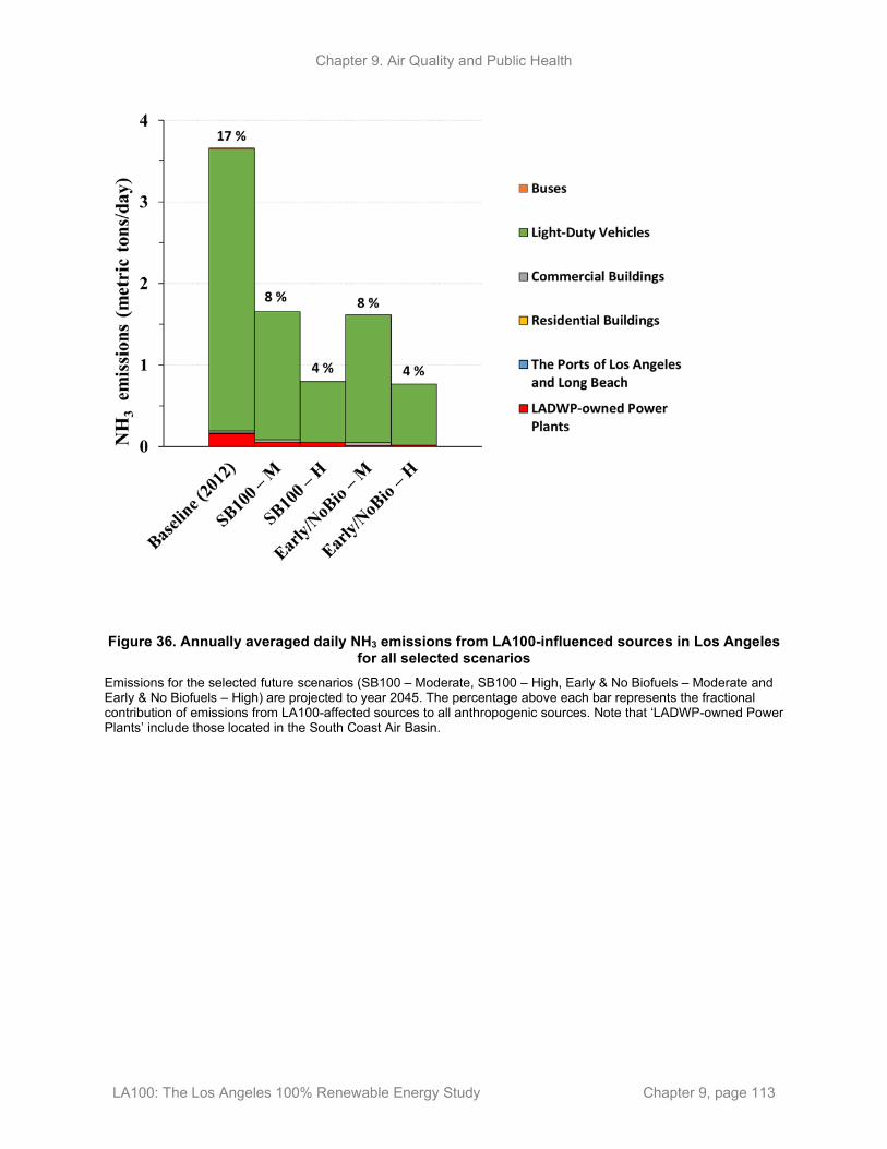
Chapter 9. Air Quality and Public Health
LA100: The Los Angeles 100% Renewable Energy Study Chapter 9, page 113
Figure 36. Annually averaged daily NH3 emissions from LA100-influenced sources in Los Angeles
for all selected scenarios Emissions for the selected future scenarios (SB100 – Moderate, SB100 – High, Early & No Biofuels – Moderate and Early & No Biofuels – High) are projected to year 2045. The percentage above each bar represents the fractional contribution of emissions from LA100-affected sources to all anthropogenic sources. Note that ‘LADWP-owned Power Plants’ include those located in the South Coast Air Basin.

Chapter 9. Air Quality and Public Health
LA100: The Los Angeles 100% Renewable Energy Study Chapter 9, page 114
Table 33. Annually Averaged Daily NH3 Emissions (metric tons/day) from LA100-Influenced Sources in Los Angeles and Citywide Total Emissions for all Selected Scenarios
Percentages in the parentheses show the percentage contribution of emissions from an LA100-influenced source to citywide total emissions in a scenario. Future scenarios are projected to year 2045.
Panel (a)
LADWP-Owned Power Plants
The Ports of LA and LB
Residential Buildings
Commercial Buildings LDVs Buses
Baseline (2012) 0.16 (0.7%) 0.01 (0.05%) 0 0.02 (0.1%) 3.5
(16%) 0.01
(0.06%)
SB100 – Moderate 0.05 (0.2%) 0 0 0.03 (0.2%) 1.6
(8%) 0
SB100 – High 0.05 (0.2%) 0 0 0.001
(0.004%) 0.8
(4%) 0
Early & No Biofuels – Moderate 0.01 (0.07%) 0 0 0.03 (0.2%)
1.6 (8%) 0
Early & No Biofuels – High 0.02 (0.09%) 0 0
0.001 (0.004%)
0.8 (4%) 0
Panel (b)
Total Emissions from LA100-influenced Sectors
Citywide Total Emissions
Baseline (2012) 3.7 22
SB100 – Moderate 1.6 21
SB100 – High 0.79 20
Early & No Biofuels – Moderate 1.6 21
Early & No Biofuels – High 0.77 20

Chapter 9. Air Quality and Public Health
LA100: The Los Angeles 100% Renewable Energy Study Chapter 9, page 115
B.9 Comparison of Simulated O3 and PM2.5 Concentrations among Baseline (2012), SB100 – Moderate, and Early & No Biofuels – High for Los Angeles
Figure 37. Spatial pattern of simulated July daily maximum 8-hour average O3 concentrations in Los Angeles for (a) Baseline (2012), (b) SB100 – Moderate minus Baseline (2012), and (c) Early &
No Biofuels – High minus Baseline (2012)
Figure 38. Spatial pattern of PM2.5 concentrations in Los Angeles for (a) Baseline (2012), (b) SB100
– Moderate minus Baseline (2012), and (c) Early & No Biofuels – High minus Baseline (2012)

Chapter 9. Air Quality and Public Health
LA100: The Los Angeles 100% Renewable Energy Study Chapter 9, page 116
B.10 Comparison of Simulated O3 and PM2.5 Concentration among Selected Future LA100 scenarios for the Innermost Model Domain
Figure 39. Spatial pattern of simulated July daily maximum 8-hour average O3 in the innermost
model domain for (a) SB100 – Moderate, and differences between SB100 – Moderate and (b) SB100 – High, (c) Early & No Biofuels – Moderate, and (d) Early & No Biofuels – High
Panel (b) isolates the effect of electrification of LA100-influenced sectors. Panel (c) shows the effect of shifting LADWP-owned power plants from natural gas to hydrogen. Panel (d) represents the combined effect of electrification and removing natural gas power plants.

Chapter 9. Air Quality and Public Health
LA100: The Los Angeles 100% Renewable Energy Study Chapter 9, page 117
Figure 40. Spatial pattern of simulated PM2.5 concentrations in the innermost model domain for (a) SB100 – Moderate, and differences between SB100 – Moderate and (b) SB100 – High, (c) Early &
No Biofuels – Moderate, and (d) Early & No Biofuels – High Values are averaged over the four simulated months to be representative of annual averages. Panel (b) isolates the effect of electrification of LA100-influenced sectors. Panel (c) shows the effect of shifting LADWP-owned power plants from removing natural gas generation. Panel (d) represents the combined effect of electrification and removing natural gas generation.
Chapter 9. Air Quality and Public Health
LA100: The Los Angeles 100% Renewable Energy Study Chapter 9, page 118
Appendix C. Additional Results for Health Analysis This appendix is organized into tables and figures. Below is a guide to the organization -
1. Health impacts results A. Discussion on effects of changing air quality on cardiovascular hospital
admissions and heart attacks (acute myocardial infarctions). B. District level results
i. Asthma-caused ER visits (Table 34) ii. Cardiovascular hospital admissions (Table 35 and Figure 41) iii. Heart Attacks (AMI) (Table 36 and Figure 42)
C. County level results for various health endpoints i. All-cause mortality (Table 37 and Figure 43) ii. Asthma-caused ER visits (Table 38 and Figure 44) iii. Cardiovascular hospital admissions (Table 39 and Figure 45) iv. Heart attacks (AMI) (Table 40 and Figure 46)
2. Net health valuation results at the county level (Table 41).
C.1 Effects of Changing Air Quality from Various LA100 Scenarios on Cardiovascular Hospital Admissions and Heart Attacks In this section, we present and discuss the impacts of air quality changes from the seven LA100 scenarios comparisons included in the chapter on two additional health metrics—non-fatal acute myocardial infarctions (AMI, commonly known as heart attack) and hospital admissions from all cardiovascular diseases (excluding AMI). Several epidemiological studies have suggested a positive association between exposure to particulate pollution (PM2.5 and PM10, but not gaseous pollutants) and heart attacks and other cardiovascular diseases, and thus PM2.5 is the only pollutant modeled in BenMAP and considered in our analysis for these two endpoints. Note that the heart attack incidences calculated here are those based on those patients that survive heart attacks 28 days after hospitalization, and thus not based on total number of heart attack patients.
Results for cardiovascular hospital admissions for various scenarios are shown in Table 35 and Figure 41. Compared to the Baseline (2012), we estimate a maximum of 72 fewer annual cardiovascular-related hospital admissions occur from the Early & No Biofuels – High. There are 50 annual avoided hospital admissions when comparing the Baseline (2012) to the future reference (SB100 – Moderate). The higher number of avoided hospital admissions in Early & No Biofuels – High (relative to current levels) is due to further reduction in PM2.5 concentration in this scenario compared to the SB100 – Moderate, as is also shown by the comparison of these two scenarios amongst themselves where the avoided hospital admissions in the city is 22. Among other LA100 scenarios in 2045, changes to cardiovascular-related hospital admissions are similar at each electrification projection level, no matter which power sector eligibility criteria is applied. This is because amongst LA100 scenarios in 2045, differences in which fuels (natural gas or H2) for power plants are allowed doesn’t affect PM2.5 concentration significantly.
Chapter 9. Air Quality and Public Health
LA100: The Los Angeles 100% Renewable Energy Study Chapter 9, page 119
PM2.5 concentration reduction due to changes in power sector emissions is so small that the resulting hospital admissions is less than one, as shown here (corresponding scenarios are Early & No Biofuel – High versus Early & No Biofuel – Moderate, and SB100 – High versus SB100 – Moderate).
Similar to the health benefits from cardiovascular disease, annual avoided heart attacks (AMI) are largest in the scenarios which change electrification levels in end-use sectors (from Moderate to High) (Table 36 and Figure 42). Changes in power sector, when evaluated in the same year (2045) have negligible impacts on AMI cases (first row of Figure 42). This is because natural gas combusting power plants have very little primary PM2.5 emissions, although they do contribute to secondary PM2.5 formed in the atmosphere but even that contribution is likely to be quite small. Similarly, hydrogen combusting plants are expected to emit only NOx and NH3, thus contributing to secondary PM2.5), but no emissions of primary PM2.5 are assumed. When comparing scenarios in 2045, on average six heart attack incidences are avoided from improving air quality due to high end-use electrification scenarios compared to the moderate end-use electrification scenarios (second row in Figure 42). When comparing to the Baseline (2012), 19 fewer heart attack cases occur in 2045 in the Early & No Biofuel – High scenario and 13 fewer cases in the future reference (SB100 – Moderate) in 2045 (third row in Figure 42).

Chapter 9. Air Quality and Public Health
LA100: The Los Angeles 100% Renewable Energy Study Chapter 9, page 120
Figure 41. Change in incidences of cardiovascular hospital admissions in Los Angeles for various scenarios
compared Among various future scenarios compared, largest benefits are observed when there is high level of electrification in the end-use
sector. Note that y-axis scale in top row is different than the rest.

Chapter 9. Air Quality and Public Health
LA100: The Los Angeles 100% Renewable Energy Study Chapter 9, page 121
Figure 42. Change in incidences of heart attacks (AMI) in Los Angeles for various scenarios compared
Among various future scenarios compared, largest benefits are observed when there is high level of electrification in the end-use sector. Note that y-axis scale in top row is different than the rest.

Chapter 9. Air Quality and Public Health
LA100: The Los Angeles 100% Renewable Energy Study Chapter 9, page 122
C.2 Health Incidences Aggregated at the District Level Table 34. Incidence Changes for Asthma-Caused ER Visits in 15 LA Districts for the Seven LA100
Scenarios Compared
Dis
tric
t
Isolating the effect of changes in power sector
Isolating the effect of changes in electrification
of end- use sectors
Isolating the effect of
simultaneous changes in
power sector and high end-
use electrification
Future (2045) versus Current (2012) comparison
at two load levels
SB100 Moderate – Early & No Biofuels – Moderate
SB100 High – Early & No Biofuels –High
SB100 Moderate – SB100 High
Early & No Biofuels –Moderate – Early & No Biofuels –High
SB100 Moderate – Early & No Biofuels –High
Baseline (2012) – SB100 Moderate
Baseline (2012) – Early & No Biofuels –High
01 0 (0 - 0) 0 (0 - 0) 2 (-1 - 4) 2 (-1 - 4) 2 (-1 - 4) -5 (-4 - -6) -4 (-5 - -2)
02 0 (0 - 0) 0 (0 - 0) 1 (-1 - 3) 1 (-1 - 3) 1 (-1 - 3) -1 (-3 - 0) 0 (-3 - 3)
03 0 (0 - 0) 0 (0 - 0) 1 (-0 - 2) 1 (-0 - 2) 1 (-0 - 2) 4 (-1 - 8) 5 (-1 - 10)
04 0 (0 - 0) 0 (0 - 0) 1 (-1 - 3) 1 (-1 - 3) 1 (-1 - 3) -3 (-3 - -3) -2 (-4 - 0)
05 0 (0 - 0) 0 (0 - 0) 1 (-1 - 2) 1 (-1 - 2) 1 (-1 - 2) -1 (-2 - -1) -1 (-2 - 1)
06 0 (0 - 0) 0 (0 - 0) 1 (-1 - 3) 1 (-1 - 3) 1 (-1 - 4) -0 (-3 - 3) 1 (-3 - 6)
07 0 (0 - 0) 0 (0 - 0) 1 (-0 - 3) 1 (-0 - 3) 1 (-0 - 3) -2 (-3 - -2) -1 (-4 - 1)
08 0 (0 - 0) 0 (0 - 0) 1 (-1 - 3) 1 (-1 - 3) 1 (-1 - 3) -2 (-3 - -2) -1 (-3 - 2)
09 0 (0 - 0) 0 (0 - 0) 1 (-1 - 4) 1 (-1 - 4) 1 (-1 - 4) -3 (-3 - -3) -1 (-4 - 1)
10 0 (0 - 0) 0 (0 - 0) 2 (-1 - 4) 2 (-1 - 4) 2 (-1 - 4) -4 (-3 - -4) -2 (-4 - -0)
11 0 (0 - 0) 0 (0 - 0) 1 (-1 - 2) 1 (-0 - 2) 1 (-1 - 2) -1 (-1 - -1) -0 (-2 - 2)
12 0 (0 - 0) 0 (0 - 0) 1 (-0 - 2) 1 (-0 - 2) 1 (-0 - 2) 2 (-1 - 5) 3 (-2 - 8)
13 0 (0 - 0) 0 (0 - 0) 1 (-1 - 4) 1 (-1 - 4) 1 (-1 - 4) -5 (-4 - -6) -4 (-5 - -3)
14 0 (0 - 0) 0 (0 - 0) 2 (-1 - 4) 2 (-1 - 4) 2 (-1 - 4) -6 (-5 - -8) -5 (-6 - -3)
15 0 (0 - 0) 0 (0 - 0) 1 (-0 - 2) 1 (-0 - 2) 1 (-0 - 2) -2 (-3 - -1) -1 (-3 - 1)
LA City
0 (0 - 1) 0 (0 - 1) 19 (-10 - 47)
18 (-10 - 47) 19 (-10 - 48) -30 (-40 - -20)
-11 (-51 - 27)

Chapter 9. Air Quality and Public Health
LA100: The Los Angeles 100% Renewable Energy Study Chapter 9, page 123
Table 35. Incidence Changes for all Cardiovascular (Less Myocardial) Hospital Admission in 15 LA Districts for the Seven LA100 Scenarios Compared
Dis
tric
t
Isolating the effect of changes in power sector
Isolating the effect of changes in electrification
of end- use sectors
Isolating the effect of
simultaneous changes in
power sector and high end-
use electrification
Future (2045) versus Current (2012) comparison
at two load levels
SB100 Moderate – Early & No Biofuels –Moderate
SB100 High – Early & No Biofuels –High
SB100 Moderate – SB100 High
Early & No Biofuels –Moderate – Early & No Biofuels –High
SB100 Moderate – Early & No Biofuels –High
Baseline (2012) – SB100 Moderate
Baseline (2012) – Early & No Biofuels –High
01 0 (0 - 0) 0 (0 - 0) 2 (1 - 3) 2 (1 - 3) 2 (1 - 3) 4 (2 - 6) 7 (4 - 10)
02 0 (0 - 0) 0 (0 - 0) 1 (1 - 2) 1 (1 - 2) 1 (1 - 2) 3 (2 - 5) 5 (3 - 7)
03 0 (0 - 0) 0 (0 - 0) 1 (0 - 1) 1 (0 - 1) 1 (0 - 1) 3 (1 - 4) 3 (2 - 5)
04 0 (0 - 0) 0 (0 - 0) 2 (1 - 2) 2 (1 - 2) 2 (1 - 3) 4 (2 - 5) 6 (3 - 8)
05 0 (0 - 0) 0 (0 - 0) 1 (1 - 2) 1 (1 - 2) 1 (1 - 2) 3 (2 - 4) 4 (2 - 6)
06 0 (0 - 0) 0 (0 - 0) 1 (1 - 2) 1 (1 - 2) 1 (1 - 2) 3 (2 - 5) 5 (3 - 7)
07 0 (0 - 0) 0 (0 - 0) 1 (1 - 1) 1 (1 - 1) 1 (1 - 1) 4 (2 - 5) 5 (3 - 7)
08 0 (0 - 0) 0 (0 - 0) 1 (1 - 2) 1 (1 - 2) 1 (1 - 2) 3 (1 - 4) 4 (2 - 6)
09 0 (0 - 0) 0 (0 - 0) 1 (1 - 2) 1 (1 - 2) 1 (1 - 2) 2 (1 - 3) 3 (2 - 5)
10 0 (0 - 0) 0 (0 - 0) 2 (1 - 3) 2 (1 - 3) 2 (1 - 3) 3 (2 - 5) 5 (3 - 8)
11 0 (0 - 0) 0 (0 - 0) 1 (1 - 2) 1 (1 - 2) 1 (1 - 2) 2 (1 - 3) 3 (2 - 5)
12 0 (0 - 0) 0 (0 - 0) 1 (1 - 1) 1 (1 - 1) 1 (1 - 1) 3 (2 - 4) 4 (2 - 5)
13 0 (0 - 0) 0 (0 - 0) 2 (1 - 3) 2 (1 - 3) 2 (1 - 3) 4 (2 - 6) 6 (3 - 9)
14 0 (0 - 0) 0 (0 - 0) 3 (2 - 4) 3 (2 - 4) 3 (2 - 4) 6 (3 - 8) 9 (5 - 12)
15 0 (0 - 0) 0 (0 - 0) 1 (1 - 1) 1 (1 - 1) 1 (1 - 1) 3 (2 - 4) 4 (2 - 6)
LA City
0 (0 - 1) 0 (0 - 1) 22 (13 - 32) 22 (13 - 32) 23 (13 - 33) 50 (28 - 71) 72 (41 - 100)

Chapter 9. Air Quality and Public Health
LA100: The Los Angeles 100% Renewable Energy Study Chapter 9, page 124
Table 36. Incidence Changes for Heart Attacks (Acute Myocardial Infarctions) in the 15 LA Districts for the Seven LA100 Scenarios Compared
Dis
tric
t
Isolating the effect of changes in power sector
Isolating the effect of changes in electrification
of end- use sectors
Isolating the effect of
simultaneous changes in
power sector and high end-use
electrification
Future (2045) versus Current (2012) comparison at two load
levels
SB100 Moderate – Early & No Biofuels –Moderate
SB100 High – Early & No Biofuels –High
SB100 Moderate – SB100 High
Early & No Biofuels –Moderate – Early & No Biofuels –High
SB100 Moderate – Early & No Biofuels –High
Baseline (2012) – SB100 Moderate
Baseline (2012) – Early & No Biofuels –High
01 0 (0 - 0) 0 (0 - 0) 1 (0 - 1) 1 (0 - 1) 1 (0 - 1) 1 (1 - 2) 2 (1 - 3)
02 0 (0 - 0) 0 (0 - 0) 0 (0 - 1) 0 (0 - 1) 0 (0 - 1) 1 (0 - 1) 1 (1 - 2)
03 0 (0 - 0) 0 (0 - 0) 0 (0 - 0) 0 (0 - 0) 0 (0 - 0) 1 (0 - 1) 1 (0 - 1)
04 0 (0 - 0) 0 (0 - 0) 0 (0 - 1) 0 (0 - 1) 0 (0 - 1) 1 (0 - 2) 1 (1 - 2)
05 0 (0 - 0) 0 (0 - 0) 0 (0 - 1) 0 (0 - 1) 0 (0 - 1) 1 (0 - 1) 1 (1 - 2)
06 0 (0 - 0) 0 (0 - 0) 0 (0 - 0) 0 (0 - 0) 0 (0 - 0) 1 (0 - 1) 1 (1 - 2)
07 0 (0 - 0) 0 (0 - 0) 0 (0 - 0) 0 (0 - 0) 0 (0 - 0) 1 (0 - 1) 1 (1 - 2)
08 0 (0 - 0) 0 (0 - 0) 0 (0 - 1) 0 (0 - 1) 0 (0 - 1) 1 (0 - 1) 1 (1 - 2)
09 0 (0 - 0) 0 (0 - 0) 0 (0 - 0) 0 (0 - 0) 0 (0 - 0) 1 (0 - 1) 1 (0 - 1)
10 0 (0 - 0) 0 (0 - 0) 1 (0 - 1) 1 (0 - 1) 1 (0 - 1) 1 (0 - 1) 1 (1 - 2)
11 0 (0 - 0) 0 (0 - 0) 0 (0 - 1) 0 (0 - 1) 0 (0 - 1) 1 (0 - 1) 1 (0 - 1)
12 0 (0 - 0) 0 (0 - 0) 0 (0 - 0) 0 (0 - 0) 0 (0 - 0) 1 (0 - 1) 1 (0 - 2)
13 0 (0 - 0) 0 (0 - 0) 1 (0 - 1) 1 (0 - 1) 1 (0 - 1) 1 (1 - 2) 2 (1 - 2)
14 0 (0 - 0) 0 (0 - 0) 1 (0 - 1) 1 (0 - 1) 1 (0 - 1) 2 (1 - 2) 2 (1 - 3)
15 0 (0 - 0) 0 (0 - 0) 0 (0 - 0) 0 (0 - 0) 0 (0 - 0) 1 (0 - 1) 1 (1 - 2)
LA City
0 (0 - 0) 0 (0 - 0) 6 (2 - 9) 6 (3 - 9) 6 (3 - 9) 13 (6 - 20) 19 (9 - 29)
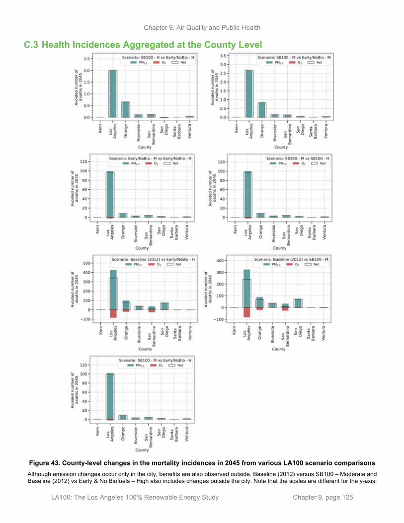
Chapter 9. Air Quality and Public Health
LA100: The Los Angeles 100% Renewable Energy Study Chapter 9, page 125
C.3 Health Incidences Aggregated at the County Level
Figure 43. County-level changes in the mortality incidences in 2045 from various LA100 scenario comparisons Although emission changes occur only in the city, benefits are also observed outside. Baseline (2012) versus SB100 – Moderate and Baseline (2012) vs Early & No Biofuels – High also includes changes outside the city. Note that the scales are different for the y-axis.

Chapter 9. Air Quality and Public Health
LA100: The Los Angeles 100% Renewable Energy Study Chapter 9, page 126
Table 37. Avoided Incidences of All-Cause Mortality from the Seven LA100 Scenarios Compared for the Counties Wholly and Partially Within the Modeling Domain
Data in parentheses show the 95% confidence interval.
County
Isolating the effect of changes in power
sector
Isolating the effect of changes in electrification
of end- use sectors
Isolating the effect of
simultaneous changes in
power sector and high end-use
electrification
Future (2045) versus Current (2012)
comparison at two load levels
SB100 Moderate – Early & No Biofuels –Moderate
SB100 High – Early & No Biofuels –High
SB100 Moderate – SB100 High
Early & No Biofuels –Moderate – Early & No Biofuels –High
SB100 Moderate – Early & No Biofuels –High
Baseline (2012) – SB100 Moderate
Baseline (2012) – Early & No Biofuels – High
Kern 0 (0 - 0) 0 (0 - 0) 0 (0 - 0) 0 (0 - 0) 0 (0 - 0) 0 (0 - 0) 0 (0 - 0)
Los Angeles
3 (2 - 4) 2 (1 - 3) 98 (66 - 130)
97 (65 - 130) 100 (67 - 130) 240 (170 - 310)
340 (240 - 440)
Orange 1 (1 - 1) 1 (0 - 1) 8 (6 - 11) 8 (6 - 11) 9 (6 - 12) 68 (48 - 87) 76 (54 - 99)
Riverside 0 (0 - 0) 0 (0 - 0) 3 (2 - 4) 3 (2 - 4) 3 (2 - 4) 37 (24 - 50) 40 (26 - 55)
San Bernardino
0 (0 - 0) 0 (0 - 0) 4 (3 - 5) 4 (3 - 5) 4 (3 - 6) 8 (8 - 7) 12 (11 - 12)
San Diego 0 (0 - 0) 0 (0 - 0) 2 (1 - 3) 2 (1 - 3) 2 (1 - 3) 71 (48 - 95) 74 (50 - 97)
Santa Barbara
0 (0 - 0) 0 (0 - 0) 0 (0 - 0) 0 (0 - 0) 0 (0 - 0) 0 (0 - 0) 0 (0 - 0)
Ventura 0 (0 - 0) 0 (0 - 0) 1 (1 - 2) 1 (1 - 2) 1 (1 - 2) -2 (-1 - -2) 0 (0 - 0)
Modeling Domain Total
4 (3 - 5) 3 (2 - 4) 120 (78 - 160)
120 (78 - 150) 120 (80 - 160) 420 (300 - 550)
540 (380 - 700)

Chapter 9. Air Quality and Public Health
LA100: The Los Angeles 100% Renewable Energy Study Chapter 9, page 127
Figure 44. County-level changes in asthma-related ER visits in 2045 from various LA100 scenario comparisons
Although emissions changes occur only in the city, benefits are also observed outside (Baseline (2012) versus SB100 – Moderate and versus Early & No Biofuels – High also includes changes outside the city). Note that the scales are different for the y-axis.
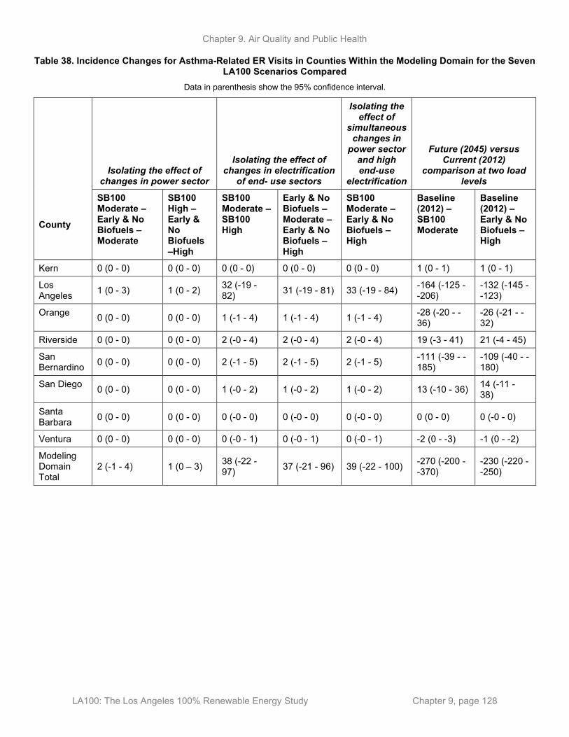
Chapter 9. Air Quality and Public Health
LA100: The Los Angeles 100% Renewable Energy Study Chapter 9, page 128
Table 38. Incidence Changes for Asthma-Related ER Visits in Counties Within the Modeling Domain for the Seven LA100 Scenarios Compared
Data in parenthesis show the 95% confidence interval.
Isolating the effect of changes in power sector
Isolating the effect of changes in electrification
of end- use sectors
Isolating the effect of
simultaneous changes in
power sector and high end-use
electrification
Future (2045) versus Current (2012)
comparison at two load levels
County
SB100 Moderate – Early & No Biofuels –Moderate
SB100 High – Early & No Biofuels –High
SB100 Moderate – SB100 High
Early & No Biofuels –Moderate – Early & No Biofuels –High
SB100 Moderate – Early & No Biofuels –High
Baseline (2012) – SB100 Moderate
Baseline (2012) – Early & No Biofuels – High
Kern 0 (0 - 0) 0 (0 - 0) 0 (0 - 0) 0 (0 - 0) 0 (0 - 0) 1 (0 - 1) 1 (0 - 1)
Los Angeles 1 (0 - 3) 1 (0 - 2) 32 (-19 -
82) 31 (-19 - 81) 33 (-19 - 84) -164 (-125 - -206)
-132 (-145 - -123)
Orange 0 (0 - 0) 0 (0 - 0) 1 (-1 - 4) 1 (-1 - 4) 1 (-1 - 4) -28 (-20 - -36)
-26 (-21 - -32)
Riverside 0 (0 - 0) 0 (0 - 0) 2 (-0 - 4) 2 (-0 - 4) 2 (-0 - 4) 19 (-3 - 41) 21 (-4 - 45)
San Bernardino 0 (0 - 0) 0 (0 - 0) 2 (-1 - 5) 2 (-1 - 5) 2 (-1 - 5) -111 (-39 - -
185) -109 (-40 - -180)
San Diego 0 (0 - 0) 0 (0 - 0) 1 (-0 - 2) 1 (-0 - 2) 1 (-0 - 2) 13 (-10 - 36) 14 (-11 - 38)
Santa Barbara 0 (0 - 0) 0 (0 - 0) 0 (-0 - 0) 0 (-0 - 0) 0 (-0 - 0) 0 (0 - 0) 0 (-0 - 0)
Ventura 0 (0 - 0) 0 (0 - 0) 0 (-0 - 1) 0 (-0 - 1) 0 (-0 - 1) -2 (0 - -3) -1 (0 - -2)
Modeling Domain Total
2 (-1 - 4) 1 (0 – 3) 38 (-22 - 97) 37 (-21 - 96) 39 (-22 - 100) -270 (-200 -
-370) -230 (-220 - -250)

Chapter 9. Air Quality and Public Health
LA100: The Los Angeles 100% Renewable Energy Study Chapter 9, page 129
Figure 45. Net change in hospital admissions (all cardiovascular, less myocardial) at county level from various
scenario compared in 2045

Chapter 9. Air Quality and Public Health
LA100: The Los Angeles 100% Renewable Energy Study Chapter 9, page 130
Table 39. Incidence Changes for Cardiovascular Hospital Admission in Counties Within the Modeling Domain for the Seven LA100 Scenarios Compared
Data in parenthesis show the 95% confidence interval.
County
Isolating the effect of changes in power sector
Isolating the effect of changes in electrification
of end- use sectors
Isolating the effect of
simultaneous changes in
power sector and high end-use
electrification
Future (2045) versus Current (2012)
comparison at two load levels
SB100 – Moderate – Early & No Biofuels – Moderate
SB100 High – Early & No Biofuels – High
SB100 Moderate – SB100 High
Early & No Biofuels –Moderate – Early & No Biofuels – High
SB100 Moderate – Early & No Biofuels – High
Baseline (2012) – SB100 Moderate
Baseline (2012) – Early & No Biofuels – High
Kern 0 (0 - 0) 0 (0 - 0) 0 (0 - 0) 0 (0 - 0) 0 (0 - 0) 0 (0 - 0) 0 (0 - 0)
Los Angeles
1 (1 - 2) 1 (0 - 1) 42 (23 - 60) 42 (23 - 60) 43 (24 - 61) 140 (76 - 200)
180 (100 - 260)
Orange 0 (0 - 0) 0 (0 - 0) 2 (1 - 4) 2 (1 - 4) 3 (2 - 4) 26 (14 - 37) 28 (16 - 41)
Riverside 0 (0 - 0) 0 (0 - 0) 1 (1 - 1) 1 (1 - 1) 1 (1 - 1) 10 (6 - 14) 11 (6 - 16)
San Bernardino
0 (0 - 0) 0 (0 - 0) 2 (1 - 2) 2 (1 - 2) 2 (1 - 2) 13 (7 - 19) 15 (8 - 21)
San Diego 0 (0 - 0) 0 (0 - 0) 1 (0 - 1) 1 (0 - 1) 1 (0 - 1) 26 (15 - 37) 27 (15 - 38)
Santa Barbara
0 (0 - 0) 0 (0 - 0) 0 (0 - 0) 0 (0 - 0) 0 (0 - 0) 0 (0 - 0) 0 (0 - 0)
Ventura 0 (0 - 0) 0 (0 - 0) 0 (0 - 1) 0 (0 - 1) 0 (0 - 1) 0 (-1 - 0) 0 (0 - 0)
Domain Total
1 (1 - 2) 1 (0 - 2) 48 (27 - 69) 48 (27 - 68) 49 (28 - 71) 210 (120 - 300)
260 (150 – 370)

Chapter 9. Air Quality and Public Health
LA100: The Los Angeles 100% Renewable Energy Study Chapter 9, page 131
Figure 46. Net change in heart attacks (acute myocardial infarctions) at county level from various scenario
compared in 2045

Chapter 9. Air Quality and Public Health
LA100: The Los Angeles 100% Renewable Energy Study Chapter 9, page 132
Table 40. Incidence Changes for Heart Attacks (Acute Myocardial Infarctions) in Counties Within the Modeling Domain for the Seven LA100 Scenarios Compared
Data in parenthesis show the 95% confidence interval.
County
Isolating the effect of changes in power sector
Isolating the effect of changes in electrification
of end- use sectors
Isolating the effect of
simultaneous changes in
power sector and high end-use
electrification
Future (2045) versus Current (2012)
comparison at two load levels
SB100 – Moderate – Early & No Biofuels – Moderate
SB100 High – Early & No Biofuels – High
SB100 Moderate – SB100 High
Early & No Biofuels –Moderate – Early & No Biofuels – High
SB100 Moderate – Early & No Biofuels – High
Baseline (2012) – SB100 Moderate
Baseline (2012) – Early & No Biofuels – High
Kern 0 (0 - 0) 0 (0 - 0) 0 (0 - 0) 0 (0 - 0) 0 (0 - 0) 0 (0 - 0) 0 (0 - 0)
Los Angeles
0 (0 - 0) 0 (0 - 0) 11 (5 - 17) 11 (5 - 17) 11 (5 - 17) 36 (17 - 54) 47 (23 - 71)
Orange 0 (0 - 0) 0 (0 - 0) 1 (0 - 1) 1 (0 - 1) 1 (0 - 1) 7 (4 - 11) 8 (4 - 12)
Riverside 0 (0 - 0) 0 (0 - 0) 0 (0 - 0) 0 (0 - 0) 0 (0 - 0) 3 (2 - 5) 4 (2 - 6)
San Bernardino
0 (0 - 0) 0 (0 - 0) 1 (0 - 1) 1 (0 - 1) 1 (0 - 1) 4 (2 - 7) 5 (2 - 8)
San Diego 0 (0 - 0) 0 (0 - 0) 0 (0 - 0) 0 (0 - 0) 0 (0 - 0) 6 (3 - 9) 6 (3 - 9)
Santa Barbara
0 (0 - 0) 0 (0 - 0) 0 (0 - 0) 0 (0 - 0) 0 (0 - 0) 0 (0 - 0) 0 (0 - 0)
Ventura 0 (0 - 0) 0 (0 - 0) 0 (0 - 0) 0 (0 - 0) 0 (0 - 0) 0 (0 - 0) 0 (0 - 0)
Domain Total
0 (0 - 1) 0 (0 - 1) 13 (6 - 19) 13 (6 - 19) 13 (6 - 20) 57 (27 - 86) 70 (34 – 110)

Chapter 9. Air Quality and Public Health
LA100: The Los Angeles 100% Renewable Energy Study Chapter 9, page 133
C.4 Valuation of Health Benefits Table 41. Valuation of Health Benefits from Avoided Mortality and Morbidity for the Seven Scenarios Compared
(in $ Million using 2019 U.S. Dollars) at the County Level Data in parenthesis show the 95% confidence interval.
Isolating the effect of changes in power sector
Isolating the effect of changes in
electrification of end- use sectors
Isolating the effect of
simultaneous changes in
power sector and high end-use
electrification
Future (2045) versus Current (2012) comparison
at two load levels
County SB100 Moderate – Early & No Biofuels –Moderate
SB100 High – Early & No Biofuels –High
SB100 Moderate – SB100 High
Early & No Biofuels –Moderate – Early & No Biofuels – High
SB100 Moderate – Early & No Biofuels – High
Baseline (2012) – SB100 Moderate
Baseline (2012) – Early & No Biofuels – High
Kern 0 (0 - 0) 0 (0 - 0) 0 (0 - 0) 0 (0 - 0) 0 (0 - 0) 2 (0 - 6) 2 (0 - 6)
Los Angeles
25 (2 - 69) 19 (-0 - 53) 910 (16 – 2,600)
910 (16 – 2,500)
930 (18 – 2,600)
2,300 (-2,200 – 8,400)
3,200 (-2,100 – 11,000)
Orange 8 (0 - 22) 6 (0 - 17) 78 (-1 - 220)
76 (-0 - 220)
84 (-1 - 240) 630 (-500 – 2,300)
720 (-500 – 2,500)
Riverside 1 (0 - 4) 1 (0 - 3) 29 (2 - 79) 28 (2 - 78) 30 (3 - 82) 350 (-98 – 11,00)
380 (-94 – 1,200)
San Bernardino
1 (-0 - 4) 1 (0 - 3) 38 (1 - 110) 38 (1 - 110) 40 (1 - 110) 72 (-1,100 – 1,300)
110 (-1,100 – 1,400)
San Diego 0 (0 - 2) 0 (-1 - 1) 20 (2 - 54) 19 (2 - 52) 20 (2 - 54) 670 (-68 – 19,00)
690 (-63 – 2,000)
Santa Barbara
0 (0 - 0) 0 (0 - 0) 0 (0 - 0) 0 (0 - 0) 0 (0 - 0) 0 (0 - 1) 0 (0 - 1)
Ventura 0 (0 - 1) 0 (0 - 1) 13 (1 - 34) 13 (1 - 34) 13 (1 - 35) -15 (-150 - 110)
-2 (-140 - 140)
Domain Total
36 (1 - 100) 27 (-1 -78) 1,100 (21 – 3,100)
1,100 (21 – 3,000)
1,100 (24 – 3,100)
4,000 (-4,100 – 15,000)
5,100 (-4,000 – 18,000)

NREL is a national laboratory of the U.S. Department of Energy Office of Energy Efficiency & Renewable Energy Operated by the Alliance for Sustainable Energy, LLC
This report is available at no cost from the National Renewable Energy Laboratory (NREL) at www.nrel.gov/publications.
Contract No. DE-AC36-08GO28308
Strategic Partnership Project Report NREL/TP-6A20-79444-9 March 2021