chapter 9 the analysis of competitive marketscc.kangwon.ac.kr/~kimoon/mi/pynd-6/im/ch09.pdf ·...
TRANSCRIPT
Chapter 9: The Analysis of Competitive Markets
117
CHAPTER 9
THE ANALYSIS OF COMPETITIVE MARKETS
REVIEW QUESTIONS
1. What is meant by deadweight loss? Why does a price ceiling usually result in a
deadweight loss?
Deadweight loss refers to the benefits lost to either consumers or producers when
markets do not operate efficiently. The term deadweight denotes that these are
benefits unavailable to any party. A price ceiling will tend to result in a deadweight
loss because at any price below the market equilibrium price, quantity supplied will be
below the market equilibrium quantity supplied, resulting in a loss of surplus to
producers. Consumers will purchase less than the market equilibrium quantity,
resulting in a loss of surplus to consumers. Consumers will also purchase less than the
quantity they demand at the price set by the ceiling. The surplus lost by consumers
and producers is not captured by either group, and surplus not captured by market
participants is deadweight loss.
2. Suppose the supply curve for a good is completely inelastic. If the government imposed
a price ceiling below the market-clearing level, would a deadweight loss result? Explain.
When the supply curve is completely inelastic, the imposition of an effective price
ceiling transfers all loss in producer surplus to consumers. Consumer surplus
increases by the difference between the market-clearing price and the price ceiling
times the market-clearing quantity. Consumers capture all decreases in total revenue.
Therefore, no deadweight loss occurs.
3. How can a price ceiling make consumers better off? Under what conditions might it
make them worse off?
If the supply curve is perfectly inelastic a price ceiling will increase consumer surplus.
If the demand curve is inelastic, price controls may result in a net loss of consumer
surplus because consumers willing to pay a higher price are unable to purchase the
price-controlled good or service. The loss of consumer surplus is greater than the
transfer of producer surplus to consumers. If demand is elastic (and supply is
relatively inelastic) consumers in the aggregate will enjoy an increase in consumer
surplus.
4. Suppose the government regulates the price of a good to be no lower than some
minimum level. Can such a minimum price make producers as a whole worse off? Explain.
Because a higher price increases revenue and decreases demand, some consumer
surplus is transferred to producers but some producer revenue is lost because
consumers purchase less. The problem with a price floor or minimum price is that it
sends the wrong signal to producers. Thinking that more should be produced as the
price goes up, producers incur extra cost to produce more than what consumers are
willing to purchase at these higher prices. These extra costs can overwhelm gains
captured in increased revenues. Thus, unless all producers decrease production, a
minimum price can make producers as a whole worse off.
5. How are production limits used in practice to raise the prices of the following goods or
services: (a) taxi rides, (b) drinks in a restaurant or bar, (c) wheat or corn?
Municipal authorities usually regulate the number of taxis through the issuance of
licenses. When the number of taxis is less than it would be without regulation, those
taxis in the market may charge a higher-than-competitive price.
State authorities usually regulate the number of liquor licenses. By requiring that any
bar or restaurant that serves alcohol have a liquor license and then limiting the
number of licenses available, the State limits entry by new bars and restaurants. This
Chapter 9: The Analysis of Competitive Markets
118
limitation allows those establishments that have a license to charge a higher price for
alcoholic beverages.
Federal authorities usually regulate the number of acres of wheat or corn in production
by creating acreage limitation programs that give farmers financial incentives to leave
some of their acreage idle. This reduces supply, driving up the price of wheat or corn.
6. Suppose the government wants to increase farmers’ incomes. Why do price supports or
acreage limitation programs cost society more than simply giving farmers money?
Price supports and acreage limitations cost society more than the dollar cost of these
programs because the higher price that results in either case will reduce quantity
demanded and hence consumer surplus, leading to a deadweight loss because the
farmer is not able to capture the lost surplus. Giving the farmers money does not
result in any deadweight loss, but is merely a redistribution of surplus from one group
to the other.
7. Suppose the government wants to limit imports of a certain good. Is it preferable to use
an import quota or a tariff? Why?
Changes in domestic consumer and producer surpluses are the same under import
quotas and tariffs. There will be a loss in (domestic) total surplus in either case.
However, with a tariff, the government can collect revenue equal to the tariff times the
quantity of imports and these revenues can be redistributed in the domestic economy
to offset the domestic deadweight loss by, for example, reducing taxes. Thus, there is
less of a loss to the domestic society as a whole. With the import quota, foreign
producers can capture the difference between the domestic and world price times the
quantity of imports. Therefore, with an import quota, there is a loss to the domestic
society as a whole. If the national government is trying to increase welfare, it should
use a tariff.
8. The burden of a tax is shared by producers and consumers. Under what conditions will
consumers pay most of the tax? Under what conditions will producers pay most of it?
What determines the share of a subsidy that benefits consumers?
The burden of a tax and the benefits of a subsidy depend on the elasticities of demand
and supply. If the ratio of the elasticity of demand to the elasticity of supply is small,
the burden of the tax falls mainly on consumers. On the other hand, if the ratio of the
elasticity of demand to the elasticity of supply is large, the burden of the tax falls
mainly on producers. Similarly, the benefit of a subsidy accrues mostly to consumers
(producers) if the ratio of the elasticity of demand to the elasticity of supply is small
(large).
9. Why does a tax create a deadweight loss? What determines the size of this loss?
A tax creates deadweight loss by artificially increasing price above the free market
level, thus reducing the equilibrium quantity. This reduction in demand reduces
consumer as well as producer surplus. The size of the deadweight loss depends on the
elasticities of supply and demand. As the elasticity of demand increases and the
elasticity of supply decreases, i.e., as supply becomes more inelastic, the deadweight
loss becomes larger.
EXERCISES
1. In 1996, the U.S. Congress raised the minimum wage from $4.25 per hour to $5.15 per
hour. Some people suggested that a government subsidy could help employers finance
the higher wage. This exercise examines the economics of a minimum wage and wage
subsidies. Suppose the supply of low-skilled labor is given by L wS
= 10 , where LS is the
quantity of low-skilled labor (in millions of persons employed each year) and w is the
wage rate (in dollars per hour). The demand for labor is given by L wD
= 80 - 10 .
Chapter 9: The Analysis of Competitive Markets
119
a. What will the free market wage rate and employment level be? Suppose the
government sets a minimum wage of $5 per hour. How many people would then be
employed?
In a free-market equilibrium, LS = LD. Solving yields w = $4 and LS = LD = 40. If the
minimum wage is $5, then LS = 50 and LD = 30. The number of people employed will be
given by the labor demand, so employers will hire 30 million workers.
LS
LD
30 40 50
8
5
4
80L
W
Figure 9.1.a
Chapter 9: The Analysis of Competitive Markets
120
b. Suppose that instead of a minimum wage, the government pays a subsidy of $1 per
hour for each employee. What will the total level of employment be now? What
will the equilibrium wage rate be?
Let w denote the wage received by the employee. Then the employer receiving the $1
subsidy per worker hour only pays w-1 for each worker hour. As shown in Figure
9.1.b, the labor demand curve shifts to:
LD = 80 - 10 (w-1) = 90 - 10w,
where w represents the wage received by the employee.
The new equilibrium will be given by the intersection of the old supply curve with the
new demand curve, and therefore, 90-10W** = 10W**, or w** = $4.5 per hour and L**
= 10(4.5) = 45 million persons employed. The real cost to the employer is $3.5 per
hour.
WL = 10w
s
9
8
4.5
4
40 45 80 90
wage and employment
after subsidy
L = 90-10wD
(subsidy)
L = 80-10wD
L
Figure 9.1.b
2. Suppose the market for widgets can be described by the following equations:
Demand: P = 10 - Q Supply: P = Q - 4
where P is the price in dollars per unit and Q is the quantity in thousands of units.
a. What is the equilibrium price and quantity?
To find the equilibrium price and quantity, equate supply and demand and solve for
QEQ:
10 - Q = Q - 4, or QEQ = 7.
Substitute QEQ into either the demand equation or the supply equation to obtain PEQ.
PEQ = 10 - 7 = 3,
or
PEQ = 7 - 4 = 3.
b. Suppose the government imposes a tax of $1 per unit to reduce widget consumption
and raise government revenues. What will the new equilibrium quantity be? What
price will the buyer pay? What amount per unit will the seller receive?
With the imposition of a $1.00 tax per unit, the demand curve for widgets shifts inward.
At each price, the consumer wishes to buy less. Algebraically, the new demand
function is:
P = 9 - Q.
Chapter 9: The Analysis of Competitive Markets
121
The new equilibrium quantity is found in the same way as in (2a):
9 - Q = Q - 4, or Q* = 6.5.
To determine the price the buyer pays, PB* , substitute Q* into the demand equation:
PB* = 10 - 6.5 = $3.50.
To determine the price the seller receives, PS* , substitute Q* into the supply equation:
PS* = 6.5 - 4 = $2.50.
c. Suppose the government has a change of heart about the importance of widgets to
the happiness of the American public. The tax is removed and a subsidy of $1 per
unit is granted to widget producers. What will the equilibrium quantity be? What
price will the buyer pay? What amount per unit (including the subsidy) will the
seller receive? What will be the total cost to the government?
The original supply curve for widgets was P = Q - 4. With a subsidy of $1.00 to widget
producers, the supply curve for widgets shifts outward. Remember that the supply
curve for a firm is its marginal cost curve. With a subsidy, the marginal cost curve
shifts down by the amount of the subsidy. The new supply function is:
P = Q - 5.
To obtain the new equilibrium quantity, set the new supply curve equal to the demand
curve:
Q - 5 = 10 - Q, or Q = 7.5.
The buyer pays P = $2.50, and the seller receives that price plus the subsidy, i.e., $3.50.
With quantity of 7,500 and a subsidy of $1.00, the total cost of the subsidy to the
government will be $7,500.
3. Japanese rice producers have extremely high production costs, in part due to the high
opportunity cost of land and to their inability to take advantage of economies of large-scale
production. Analyze two policies intended to maintain Japanese rice production: (1) a per-
pound subsidy to farmers for each pound of rice produced, or (2) a per-pound tariff on
imported rice. Illustrate with supply-and-demand diagrams the equilibrium price and
quantity, domestic rice production, government revenue or deficit, and deadweight loss
from each policy. Which policy is the Japanese government likely to prefer? Which policy
are Japanese farmers likely to prefer?
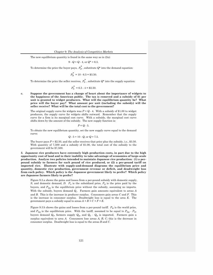
Figure 9.3.a shows the gains and losses from a per-pound subsidy with domestic supply,
S, and domestic demand, D. PS is the subsidized price, PB is the price paid by the
buyers, and PEQ is the equilibrium price without the subsidy, assuming no imports.
With the subsidy, buyers demand Q1. Farmers gain amounts equivalent to areas A
and B. This is the increase in producer surplus. Consumers gain areas C and F. This
is the increase in consumer surplus. Deadweight loss is equal to the area E. The
government pays a subsidy equal to areas A + B + C + F + E.
Figure 9.3.b shows the gains and losses from a per-pound tariff. PW is the world price,
and PEQ is the equilibrium price. With the tariff, assumed to be equal to PEQ - PW,
buyers demand QT, farmers supply QD, and QT - QD is imported. Farmers gain a
surplus equivalent to area A. Consumers lose areas A, B, C; this is the decrease in
consumer surplus. Deadweight loss is equal to the areas B and C.
Chapter 9: The Analysis of Competitive Markets
122
Price
Quantity
S
D
PB
PEQ
PS
A
C
B
E
F
QEQ Q1
Figure 9.3.a
Price
S
D
PEQ
PW
A CB
QEQ QTQD Quantity
Figure 9.3.b
Without more information regarding the size of the subsidy and the tariff, and the
specific equations for supply and demand, it seems sensible to assume that the
Japanese government would avoid paying subsidies by choosing a tariff, but the rice
farmers would prefer the subsidy.
4. In 1983, the Reagan Administration introduced a new agricultural program called the
Payment-in-Kind Program. To see how the program worked, let’s consider the wheat
market.
a. Suppose the demand function is QD = 28 - 2P and the supply function is Q
S = 4 + 4P,
where P is the price of wheat in dollars per bushel and Q is the quantity in billions
of bushels. Find the free-market equilibrium price and quantity.
Equating demand and supply, QD = Q
S,
28 - 2P = 4 + 4P, or P = 4.
Chapter 9: The Analysis of Competitive Markets
123
To determine the equilibrium quantity, substitute P = 4 into either the supply equation
or the demand equation:
QS = 4 + 4(4) = 20
and
QD = 28 - 2(4) = 20.
b. Now suppose the government wants to lower the supply of wheat by 25 percent from
the free-market equilibrium by paying farmers to withdraw land from production.
However, the payment is made in wheat rather than in dollars--hence the name of
the program. The wheat comes from the government’s vast reserves that resulted
from previous price-support programs. The amount of wheat paid is equal to the
amount that could have been harvested on the land withdrawn from production.
Farmers are free to sell this wheat on the market. How much is now produced by
farmers? How much is indirectly supplied to the market by the government? What
is the new market price? How much do the farmers gain? Do consumers gain or
lose?
Because the free market supply by farmers is 20 billion bushels, the 25 percent
reduction required by the new Payment-In-Kind (PIK) Program would imply that the
farmers now produce 15 billion bushels. To encourage farmers to withdraw their land
from cultivation, the government must give them 5 billion bushels, which they sell on
the market.
Because the total supply to the market is still 20 billion bushels, the market price does
not change; it remains at $4 per bushel. The farmers gain $20 billion, equal to ($4)(5
billion bushels), from the PIK Program, because they incur no costs in supplying the
wheat (which they received from the government) to the market. The PIK program
does not affect consumers in the wheat market, because they purchase the same
amount at the same price as they did in the free market case.
c. Had the government not given the wheat back to the farmers, it would have stored
or destroyed it. Do taxpayers gain from the program? What potential problems does
the program create?
Taxpayers gain because the government is not required to store the wheat. Although
everyone seems to gain from the PIK program, it can only last while there are
government wheat reserves. The PIK program assumes that the land removed from
production may be restored to production when stockpiles are exhausted. If this
cannot be done, consumers may eventually pay more for wheat-based products.
5. About 100 million pounds of jelly beans are consumed in the United States each year,
and the price has been about 50 cents per pound. However, jelly bean producers feel that
their incomes are too low, and they have convinced the government that price supports are
in order. The government will therefore buy up as many jelly beans as necessary to keep
the price at $1 per pound. However, government economists are worried about the impact
of this program, because they have no estimates of the elasticities of jelly bean demand or
supply.
a. Could this program cost the government more than $50 million per year? Under
what conditions? Could it cost less than $50 million per year? Under what
conditions? Illustrate with a diagram.
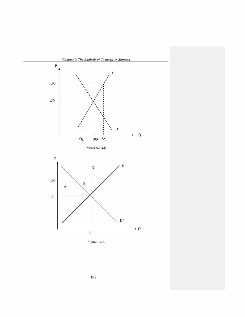
If the quantities demanded and supplied are very responsive to price changes, then a
government program that doubles the price of jelly beans could easily cost more than
$50 million. In this case, the change in price will cause a large change in quantity
supplied, and a large change in quantity demanded. In Figure 9.5.a.i, the cost of the
program is (QS-QD)*$1. Given QS-QD is larger than 50 million, then the government
will pay more than 50 million dollars. If instead supply and demand were relatively
price inelastic, then the change in price would result in very small changes in quantity
Chapter 9: The Analysis of Competitive Markets
124
supplied and quantity demanded and (QS-QD) would be less than $50 million, as
illustrated in figure 9.5.a.ii.
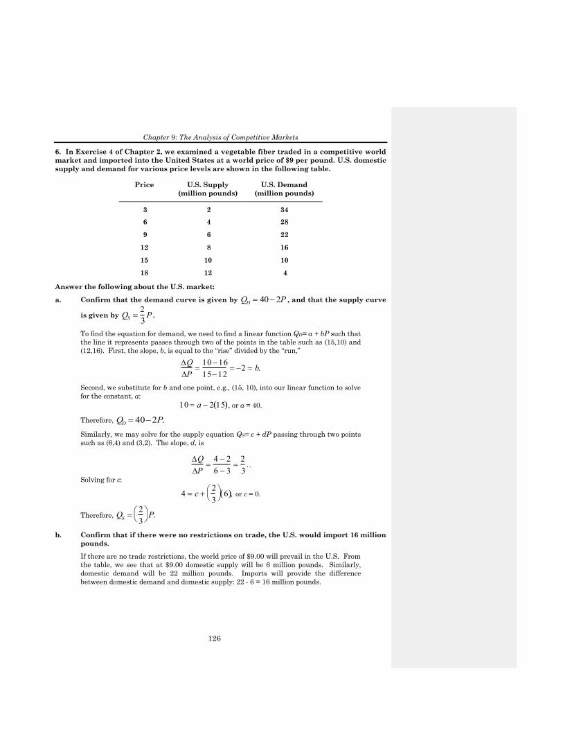
b. Could this program cost consumers (in terms of lost consumer surplus) more than $50
million per year? Under what conditions? Could it cost consumers less than $50
million per year? Under what conditions? Again, use a diagram to illustrate.
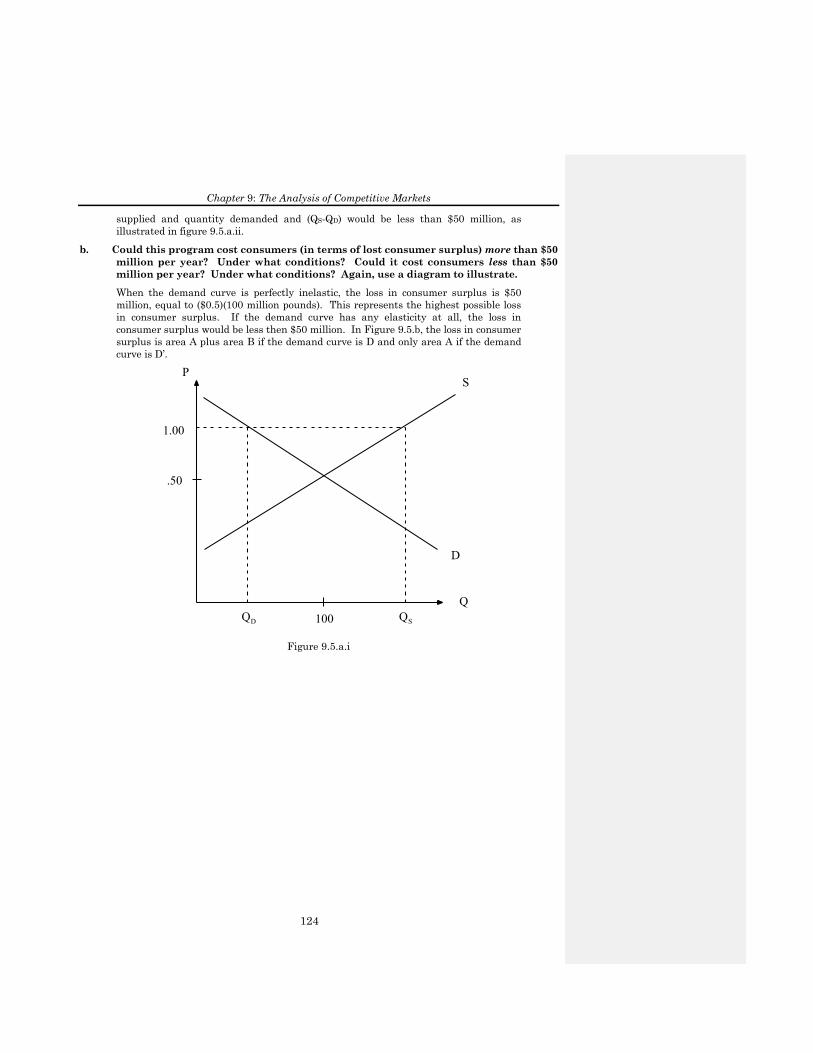
When the demand curve is perfectly inelastic, the loss in consumer surplus is $50
million, equal to ($0.5)(100 million pounds). This represents the highest possible loss
in consumer surplus. If the demand curve has any elasticity at all, the loss in
consumer surplus would be less then $50 million. In Figure 9.5.b, the loss in consumer
surplus is area A plus area B if the demand curve is D and only area A if the demand
curve is D’.
Q
P
QSQD
1.00
.50
100
D
S
Figure 9.5.a.i
Chapter 9: The Analysis of Competitive Markets
125
Q
P
QSQD
1.00
.50
100
D
S
Figure 9.5.a.ii
Q
P
D’
DS
AB
100
1.00
.50
Figure 9.5.b
Chapter 9: The Analysis of Competitive Markets
126
6. In Exercise 4 of Chapter 2, we examined a vegetable fiber traded in a competitive world
market and imported into the United States at a world price of $9 per pound. U.S. domestic
supply and demand for various price levels are shown in the following table.
Price U.S. Supply
(million pounds)
U.S. Demand
(million pounds)
3 2 34
6 4 28
9 6 22
12 8 16
15 10 10
18 12 4
Answer the following about the U.S. market:
a. Confirm that the demand curve is given by
QD 40 2P , and that the supply curve
is given by
QS 2
3P .
To find the equation for demand, we need to find a linear function QD= a + bP such that
the line it represents passes through two of the points in the table such as (15,10) and
(12,16). First, the slope, b, is equal to the “rise” divided by the “run,”
Q
P
1016
1512 2 b.
Second, we substitute for b and one point, e.g., (15, 10), into our linear function to solve
for the constant, a:
10 a 2 15 , or a = 40.
Therefore, QD 402P.
Similarly, we may solve for the supply equation QS= c + dP passing through two points
such as (6,4) and (3,2). The slope, d, is
Q
P
4 2
6 3
2
3. .
Solving for c:
4 c 2
3
6 , or c = 0.
Therefore, QS 2
3
P.
b. Confirm that if there were no restrictions on trade, the U.S. would import 16 million
pounds.
If there are no trade restrictions, the world price of $9.00 will prevail in the U.S. From
the table, we see that at $9.00 domestic supply will be 6 million pounds. Similarly,
domestic demand will be 22 million pounds. Imports will provide the difference
between domestic demand and domestic supply: 22 - 6 = 16 million pounds.
Chapter 9: The Analysis of Competitive Markets
127
c. If the United States imposes a tariff of $3 per pound, what will be the U.S. price and
level of imports? How much revenue will the government earn from the tariff? How
large is the deadweight loss?
With a $3.00 tariff, the U.S. price will be $12 (the world price plus the tariff). At this
price, demand is 16 million pounds and supply is 8 million pounds, so imports are 8
million pounds (16-8). The government will collect $3*8=$24 million. The deadweight
loss is equal to
0.5(12-9)(8-6)+0.5(12-9)(22-16)=$12 million.
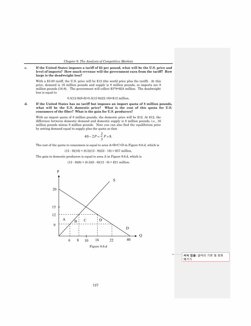
d. If the United States has no tariff but imposes an import quota of 8 million pounds,
what will be the U.S. domestic price? What is the cost of this quota for U.S.
consumers of the fiber? What is the gain for U.S. producers?
With an import quota of 8 million pounds, the domestic price will be $12. At $12, the
difference between domestic demand and domestic supply is 8 million pounds, i.e., 16
million pounds minus 8 million pounds. Note you can also find the equilibrium price
by setting demand equal to supply plus the quota so that
40 2P 2
3P 8.
The cost of the quota to consumers is equal to area A+B+C+D in Figure 9.6.d, which is
(12 - 9)(16) + (0.5)(12 - 9)(22 - 16) = $57 million.
The gain to domestic producers is equal to area A in Figure 9.6.d, which is
(12 - 9)(6) + (0.5)(8 - 6)(12 - 9) = $21 million.
6 8 10 16 22
9
12
15
S
D
Q
P
AB C D
20
40
Figure 9.6.d
서식 있음: 글머리 기호 및 번호
매기기
Chapter 9: The Analysis of Competitive Markets
128
7.7. The United States currently imports all of its coffee. The annual demand for coffee
by U.S. consumers is given by the demand curve Q = 250 – 10P, where Q is quantity (in
millions of pounds) and P is the market price per pound of coffee. World producers can
harvest and ship coffee to US distributors at a constant marginal (= average) cost of $8
per pound. U.S. distributors can in turn distribute coffee for a constant $2 per pound.
The U.S. coffee market is competitive. Congress is considering imposing a tariff on coffee
imports of $2 per pound.
a. If there is no tariff, how much do consumers pay for a pound of coffee? What is the
quantity demanded?
If there is no tariff then consumers will pay $10 per pound of coffee, which is found
by adding the $8 that it costs to import the coffee plus the $2 that is costs to
distribute the coffee in the U.S., per pound. In a competitive market, price is equal to
marginal cost. If the price is $10, then demand is 150 million pounds.
b.b. If the tariff is imposed, how much will consumers pay for a pound of coffee? What
is the quantity demanded?
Now we must add $2 per pound to marginal cost, so price will be $12 per pound and
demand is Q=250-10(12)=130 million pounds.
c.b. Calculate the lost consumer surplus.
The lost consumer surplus is (12-10)(130)+0.5(12-10)(150-130)=$280 million.
d.d. Calculate the tax revenue collected by the government.
The tax revenue is equal to the tax of $2 per pound times the number of pounds
imported, which is 130 million pounds. Tax revenue is therefore $260 million.
e.e. Does the tariff result in a net gain or a net loss to society as a whole?
There is a net loss to society because the gain ($260 million) is less than the loss
($280 million).
8. A particular metal is traded in a highly competitive world market at a world price of $9
per ounce. Unlimited quantities are available for import into the United States at this
price. The supply of this metal from domestic U.S. mines and mills can be represented by
the equation QS = 2/3P, where Q
S is U.S. output in million ounces and P is the domestic
price. The demand for the metal in the United States is QD = 40 - 2P, where Q
D is the
domestic demand in million ounces.
In recent years, the U.S. industry has been protected by a tariff of $9 per ounce.
Under pressure from other foreign governments, the United States plans to reduce this
tariff to zero. Threatened by this change, the U.S. industry is seeking a Voluntary Restraint
Agreement that would limit imports into the United States to 8 million ounces per year.
a. Under the $9 tariff, what was the U.S. domestic price of the metal?
With a $9 tariff, the price of the imported metal on U.S. markets would be $18, the
tariff plus the world price of $9. To determine the domestic equilibrium price, equate
domestic supply and domestic demand:
2
3P = 40 - 2P, or P = $15.
The equilibrium quantity is found by substituting a price of $15 into either the demand
or supply equations:
QD 40 2 15 10
and
QS
2
3
15 10.
서식 있음: 글머리 기호 및 번호
매기기
서식 있음: 글머리 기호 및 번호
매기기
서식 있음: 글머리 기호 및 번호
매기기
서식 있음: 글머리 기호 및 번호
매기기

Chapter 9: The Analysis of Competitive Markets
129
The equilibrium quantity is 10 million ounces. Because the domestic price of $15 is
less than the world price plus the tariff, $18, there will be no imports.
b. If the United States eliminates the tariff and the Voluntary Restraint Agreement is
approved, what will be the U.S. domestic price of the metal?
With the Voluntary Restraint Agreement, the difference between domestic supply and
domestic demand would be limited to 8 million ounces, i.e. QD - Q
S = 8. To determine
the domestic price of the metal, set QD - Q
S = 8 and solve for P:
40 2P 2
3P 8, or P = $12.
At a price of $12, QD = 16 and Q
S = 8; the difference of 8 million ounces will be supplied
by imports.
9. Among the tax proposals regularly considered by Congress is an additional tax on
distilled liquors. The tax would not apply to beer. The price elasticity of supply of liquor is
4.0, and the price elasticity of demand is -0.2. The cross-elasticity of demand for beer with
respect to the price of liquor is 0.1.
a. If the new tax is imposed, who will bear the greater burden, liquor suppliers or
liquor consumers? Why?
Section 9.6 in the text provides a formula for the “pass-through” fraction, i.e., the
fraction of the tax borne by the consumer. This fraction is E
E E
S
S D, where ES is the
own-price elasticity of supply and ED is the own-price elasticity of demand.
Substituting for ES and ED, the pass-through fraction is
4
4 0.2
4
4.2 0.95.
Therefore, 95 percent of the tax is passed through to the consumers because supply is
relatively elastic and demand is relatively inelastic.
b. Assuming that beer supply is infinitely elastic, how will the new tax affect the beer
market?
With an increase in the price of liquor (from the large pass-through of the liquor tax),
some consumers will substitute away from liquor to beer, shifting the demand curve for
beer outward. With an infinitely elastic supply for beer (a perfectly flat supply curve),
there will be no change in the equilibrium price of beer.
10. In Example 9.1, we calculated the gains and losses from price controls on natural gas
and found that there was a deadweight loss of $1.4 billion. This calculation was based on a
price of oil of $8 per barrel. If the price of oil were $12 per barrel, what would the free
market price of gas be? How large a deadweight loss would result if the maximum
allowable price of natural gas were $1.00 per thousand cubic feet?
From Example 9.1, we know that the supply and demand curves for natural gas in the
1970s can be approximated as follows:
QS = 14 + 2PG + 0.25PO
and
QD = -5PG + 3.75PO,
where PG is the price of gas and PO is the price of oil.
Chapter 9: The Analysis of Competitive Markets
130
With the price of oil at $12 per barrel, these curves become,
QS = 17 + 2PG
and
QD = 45 - 5PG.
Setting quantity demanded equal to quantity supplied,
17 + 2PG = 45 - 5PG, or PG = $4.
At this price, the equilibrium quantity is 25 thousand cubic feet (Tcf).
If a ceiling of $1 is imposed, producers would supply 19 Tcf and consumers would
demand 40 Tcf. The deadweight loss is the area below the demand curve and above
the supply curve, between the quantities of 19 and 25 Tcf. This can be computed as
0.5(5.2-4)(25-19)+0.5(4-1)(25-19)=$12.6 billion.
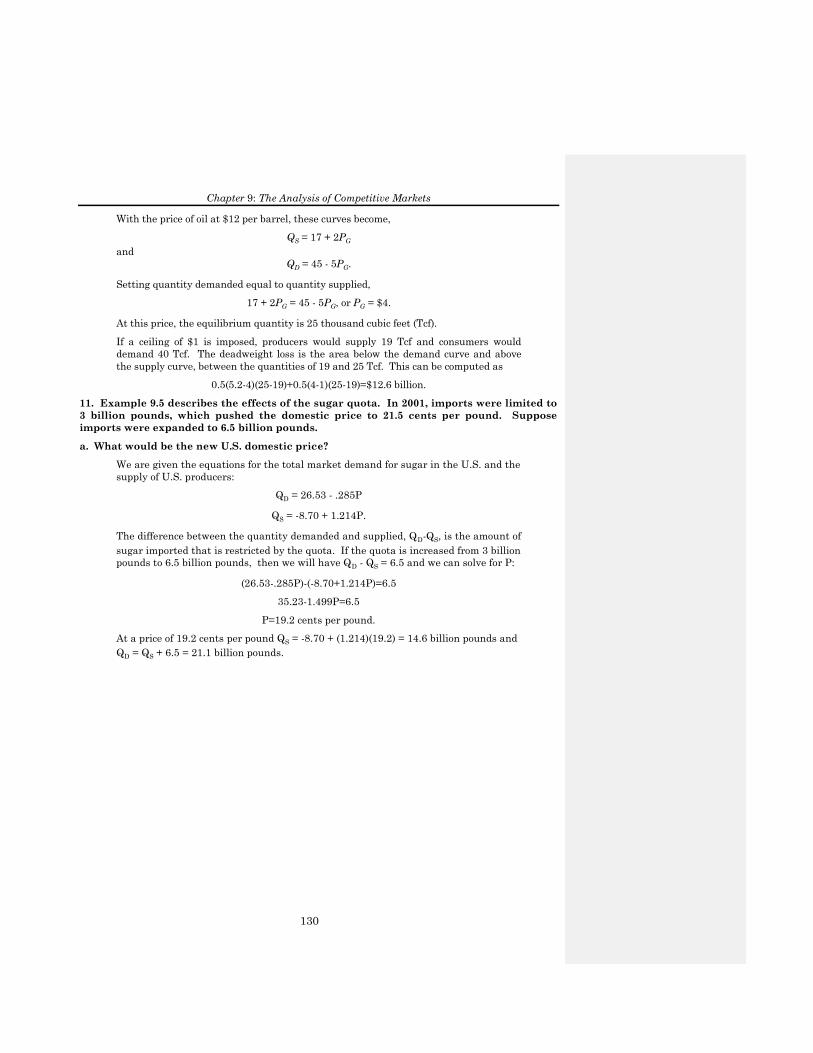
11. Example 9.5 describes the effects of the sugar quota. In 2001, imports were limited to
3 billion pounds, which pushed the domestic price to 21.5 cents per pound. Suppose
imports were expanded to 6.5 billion pounds.
a. What would be the new U.S. domestic price?
We are given the equations for the total market demand for sugar in the U.S. and the
supply of U.S. producers:
QD = 26.53 - .285P
QS = -8.70 + 1.214P.
The difference between the quantity demanded and supplied, QD-QS, is the amount of
sugar imported that is restricted by the quota. If the quota is increased from 3 billion
pounds to 6.5 billion pounds, then we will have QD - QS = 6.5 and we can solve for P:
(26.53-.285P)-(-8.70+1.214P)=6.5
35.23-1.499P=6.5
P=19.2 cents per pound.
At a price of 19.2 cents per pound QS = -8.70 + (1.214)(19.2) = 14.6 billion pounds and
QD = QS + 6.5 = 21.1 billion pounds.
Chapter 9: The Analysis of Competitive Markets
131
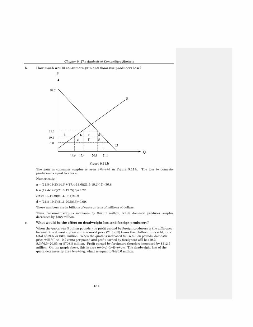
b. How much would consumers gain and domestic producers lose?
a b c d
S
D
14.6 17.4 20.4 21.1
21.5
19.2
Q
P
94.7
e f g8.3
Figure 9.11.b
The gain in consumer surplus is area a+b+c+d in Figure 9.11.b. The loss to domestic
producers is equal to area a.
Numerically:
a = (21.5-19.2)(14.6)+(17.4-14.6)(21.5-19.2)(.5)=36.8
b = (17.4-14.6)(21.5-19.2)(.5)=3.22
c = (21.5-19.2)(20.4-17.4)=6.9
d = (21.5-19.2)(21.1-20.5)(.5)=0.69.
These numbers are in billions of cents or tens of millions of dollars.
Thus, consumer surplus increases by $476.1 million, while domestic producer surplus
decreases by $368 million.
c. What would be the effect on deadweight loss and foreign producers?
When the quota was 3 billion pounds, the profit earned by foreign producers is the difference
between the domestic price and the world price (21.5-8.3) times the 3 billion units sold, for a
total of 39.6, or $396 million. When the quota is increased to 6.5 billion pounds, domestic
price will fall to 19.2 cents per pound and profit earned by foreigners will be (19.2-
8.3)*6.5=70.85, or $708.5 million. Profit earned by foreigners therefore increased by $312.5
million. On the graph above, this is area (e+f+g)-(c+f)=e+g-c. The deadweight loss of the
quota decreases by area b+e+d+g, which is equal to $420.6 million.
Chapter 9: The Analysis of Competitive Markets
132
12. The domestic supply and demand curves for hula beans are as follows:
Supply: P = 50 + Q Demand: P = 200 - 2Q
where P is the price in cents per pound and Q is the quantity in millions of pounds. The
U.S. is a small producer in the world hula bean market, where the current price (which will
not be affected by anything we do) is 60 cents per pound. Congress is considering a tariff of
40 cents per pound. Find the domestic price of hula beans that will result if the tariff is
imposed. Also compute the dollar gain or loss to domestic consumers, domestic producers,
and government revenue from the tariff.
To analyze the influence of a tariff on the domestic hula bean market, start by solving
for domestic equilibrium price and quantity. First, equate supply and demand to
determine equilibrium quantity:
50 + Q = 200 - 2Q, or QEQ = 50.
Thus, the equilibrium quantity is 50 million pounds. Substituting QEQ equals 50 into
either the supply or demand equation to determine price, we find:
PS = 50 + 50 = 100 and PD = 200 - (2)(50) = 100.
The equilibrium price P is $1 (100 cents). However, the world market price is 60 cents.
At this price, the domestic quantity supplied is 60 = 50 - QS, or QS = 10, and similarly,
domestic demand at the world price is 60 = 200 - 2QD, or QD = 70. Imports are equal to
the difference between domestic demand and supply, or 60 million pounds. If Congress
imposes a tariff of 40 cents, the effective price of imports increases to $1. At $1,
domestic producers satisfy domestic demand and imports fall to zero.
As shown in Figure 9.12, consumer surplus before the imposition of the tariff is equal
to area a+b+c, or (0.5)(200 - 60)(70) = 4,900 million cents or $49 million. After the tariff,
the price rises to $1.00 and consumer surplus falls to area a, or
(0.5)(200 - 100)(50) = $25 million, a loss of $24 million. Producer surplus will increase
by area b, or (100-60)(10)+(.5)(100-60)(50-10)=$12 million.
Finally, because domestic production is equal to domestic demand at $1, no hula beans
are imported and the government receives no revenue. The difference between the loss
of consumer surplus and the increase in producer surplus is deadweight loss, which in
this case is equal to $12 million. See Figure 9.12.
Chapter 9: The Analysis of Competitive Markets
133
7010 50
60
100
S
D
Q
P
a
b c
100
200
50
Figure 9.12
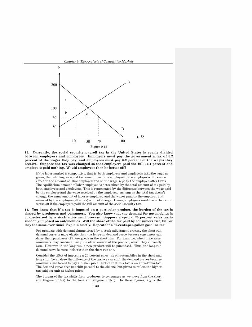
13. Currently, the social security payroll tax in the United States is evenly divided
between employers and employees. Employers must pay the government a tax of 6.2
percent of the wages they pay, and employees must pay 6.2 percent of the wages they
receive. Suppose the tax was changed so that employers paid the full 12.4 percent and
employees paid nothing. Would employees then be better off?
If the labor market is competitive, that is, both employers and employees take the wage as
given, then shifting an equal tax amount from the employee to the employer will have no
effect on the amount of labor employed and on the wage kept by the employee after taxes.
The equilibrium amount of labor employed is determined by the total amount of tax paid by
both employees and employers. This is represented by the difference between the wage paid
by the employer and the wage received by the employee. As long as the total tax doesn’t
change, the same amount of labor is employed and the wages paid by the employer and
received by the employee (after tax) will not change. Hence, employees would be no better or
worse off if the employers paid the full amount of the social security tax.
14. You know that if a tax is imposed on a particular product, the burden of the tax is
shared by producers and consumers. You also know that the demand for automobiles is
characterized by a stock adjustment process. Suppose a special 20 percent sales tax is
suddenly imposed on automobiles. Will the share of the tax paid by consumers rise, fall, or
stay the same over time? Explain briefly. Repeat for a 50-cents-per-gallon gasoline tax.
For products with demand characterized by a stock adjustment process, the short-run
demand curve is more elastic than the long-run demand curve because consumers can
delay their purchases of these goods in the short run. For example, when price rises,
consumers may continue using the older version of the product, which they currently
own. However, in the long run, a new product will be purchased. Thus, the long-run
demand curve is more inelastic than the short-run one.
Consider the effect of imposing a 20 percent sales tax on automobiles in the short and
long run. To analyze the influence of the tax, we can shift the demand curves because
consumers are forced to pay a higher price. Notice that this tax is an ad valorem tax.
The demand curve does not shift parallel to the old one, but pivots to reflect the higher
tax paid per unit at higher prices.
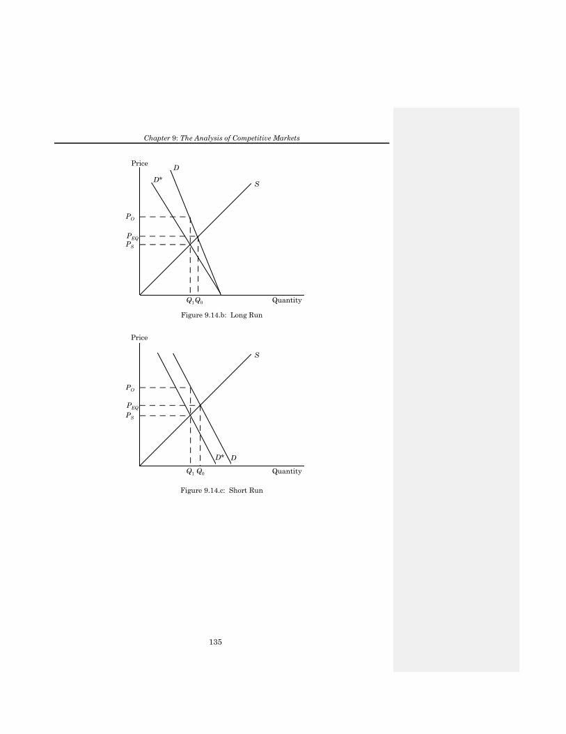
The burden of the tax shifts from producers to consumers as we move from the short
run (Figure 9.15.a) to the long run (Figure 9.15.b). In these figures, PO is the
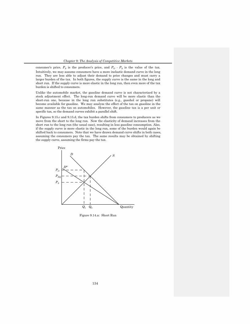
Chapter 9: The Analysis of Competitive Markets
134
consumer’s price, PS is the producer’s price, and PO - PS is the value of the tax.
Intuitively, we may assume consumers have a more inelastic demand curve in the long
run. They are less able to adjust their demand to price changes and must carry a
larger burden of the tax. In both figures, the supply curve is the same in the long and
short run. If the supply curve is more elastic in the long run, then even more of the tax
burden is shifted to consumers.
Unlike the automobile market, the gasoline demand curve is not characterized by a
stock adjustment effect. The long-run demand curve will be more elastic than the
short-run one, because in the long run substitutes (e.g., gasohol or propane) will
become available for gasoline. We may analyze the effect of the tax on gasoline in the
same manner as the tax on automobiles. However, the gasoline tax is a per unit or
specific tax, so the demand curves exhibit a parallel shift.
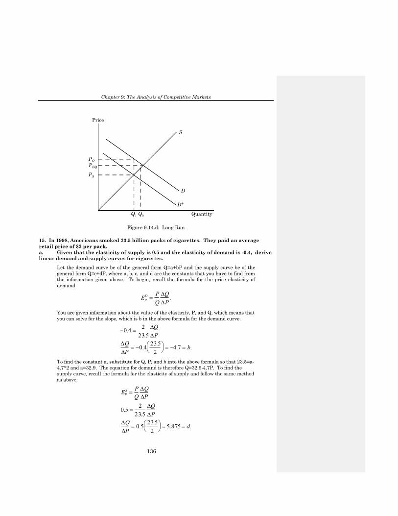
In Figures 9.15.c and 9.15.d, the tax burden shifts from consumers to producers as we
move from the short to the long run. Now the elasticity of demand increases from the
short run to the long run (the usual case), resulting in less gasoline consumption. Also,
if the supply curve is more elastic in the long run, some of the burden would again be
shifted back to consumers. Note that we have drawn demand curve shifts in both cases,
assuming the consumers pay the tax. The same results may be obtained by shifting
the supply curve, assuming the firms pay the tax.
Price
Quantity
SD
PEQ
PS
Q1 Q0
D*PO
Figure 9.14.a: Short Run
Chapter 9: The Analysis of Competitive Markets
135
Price
Quantity
S
D
PEQPS
Q1Q0
D*
PO
Figure 9.14.b: Long Run
Price
Quantity
S
D
PEQPS
Q1 Q0
D*
PO
Figure 9.14.c: Short Run
Chapter 9: The Analysis of Competitive Markets
136
Price
Quantity
S
D
PEQ
PS
Q1 Q0
D*
PO
Figure 9.14.d: Long Run
15. In 1998, Americans smoked 23.5 billion packs of cigarettes. They paid an average
retail price of $2 per pack.
a. Given that the elasticity of supply is 0.5 and the elasticity of demand is -0.4, derive
linear demand and supply curves for cigarettes.
Let the demand curve be of the general form Q=a+bP and the supply curve be of the
general form Q=c+dP, where a, b, c, and d are the constants that you have to find from
the information given above. To begin, recall the formula for the price elasticity of
demand
EPDP
Q
Q
P.
You are given information about the value of the elasticity, P, and Q, which means that
you can solve for the slope, which is b in the above formula for the demand curve.
0.4 2
23.5
Q
P
Q
P 0.4
23.5
2
4.7 b.
To find the constant a, substitute for Q, P, and b into the above formula so that 23.5=a-
4.7*2 and a=32.9. The equation for demand is therefore Q=32.9-4.7P. To find the
supply curve, recall the formula for the elasticity of supply and follow the same method
as above:
EPS
P
Q
Q
P
0.5 2
23.5
Q
P
Q
P 0.5
23.5
2
5.875 d.
Chapter 9: The Analysis of Competitive Markets
137
To find the constant c, substitute for Q, P, and d into the above formula so that
23.5=c+5.875*2 and c=11.75. The equation for supply is therefore Q=11.75+5.875P.
b. In November 1998, after settling a lawsuit filed by 46 states, the three major
tobacco companies raised the retail price of a pack of cigarettes by 45 cents. What is the
new equilibrium price and quantity? How many fewer packs of cigarettes are sold?
The new price of cigarettes would be $2.45. Plugging $2.45 into the demand curve
results in a quantity demanded of 21.39 billion packs, which represents a decrease of
2.11 billion packs of cigarettes. Note that you could also use the formula for
elasticity to come up with the answer:
pD
%Q
%P
%Q
22.5%%Q 9%.
The new quantity demanded is then 23.5*.91=21.39 billion packs.
c. Cigarettes are subject to a Federal tax, which was about 25 cents per pack in 1998.
This tax will increase by 15 cents in 2002. What will this increase do to the market-
clearing price and quantity?
The tax of 15 cents will shift the supply curve up by 15 cents. To find the new supply
curve, first rewrite the equation for the supply curve as a function of Q instead of P:
QS 11.75 5.875P P QS
5.875
11.75
5.875.
The new supply curve is now
P QS
5.875
11.75
5.875 .15 0.17QS 1.85.
To equate the new supply with the equation for demand, first rewrite demand as a
function of Q instead of P:
QD 32.94.7PP 7 .21QD.
Now equate supply and demand and solve for the equilibrium quantity:
0.17Q1.85 7 .21QQ 23.29. Plugging the equilibrium quantity into the equation for demand gives a market price
of $2.11.
Note that we assume that part c is independent of part b. If we incorporate
information from part b, the supply curve in part c is 60 cents (45+15) higher
vertically than the supply curve from part a.
d. How much of the Federal tax will consumers pay? What part will producers pay?
Since the price went up by 11 cents, consumers pay 11 of the 15 cents or 73% of the
tax, and producers will pay the remaining 27% or 4 cents.
16. 서식 있음: 글머리 기호 및 번호
매기기