chapter chapter 5 555 normal probability distributions · 2009-03-26 · 1 normal probability...
TRANSCRIPT
1
Normal Probability Normal Probability Normal Probability Normal Probability DistributionsDistributionsDistributionsDistributions
Chapter Chapter Chapter Chapter 5555
§§§§ 5555....1111
Introduction to Introduction to Introduction to Introduction to Normal Distributions Normal Distributions Normal Distributions Normal Distributions
and the Standard and the Standard and the Standard and the Standard DistributionDistributionDistributionDistribution

2
Larson & Farber, Larson & Farber, Larson & Farber, Larson & Farber, Elementary Statistics:Elementary Statistics:Elementary Statistics:Elementary Statistics: Picturing the WorldPicturing the WorldPicturing the WorldPicturing the World, , , , 3333eeee 3333
Properties of Normal DistributionsProperties of Normal DistributionsProperties of Normal DistributionsProperties of Normal Distributions
A continuous random variablecontinuous random variablecontinuous random variablecontinuous random variable has an infinite number of possible values that can be represented by an interval on the number line.
Hours spent studying in a day
0 63 9 1512 18 2421
The time spent studying can be any number between 0 and 24.
The probability distribution of a continuous random variable is called a continuous probability distribution.continuous probability distribution.continuous probability distribution.continuous probability distribution.
Larson & Farber, Larson & Farber, Larson & Farber, Larson & Farber, Elementary Statistics: Picturing the WorldElementary Statistics: Picturing the WorldElementary Statistics: Picturing the WorldElementary Statistics: Picturing the World, , , , 3333eeee 4444
Properties of Normal DistributionsProperties of Normal DistributionsProperties of Normal DistributionsProperties of Normal Distributions
The most important probability distribution in statistics is the normalnormalnormalnormal distributiondistributiondistributiondistribution.
A normal distribution is a continuous probability distribution for a random variable, x. The graph of a normal distribution is called the normalnormalnormalnormal curvecurvecurvecurve.
Normal curveNormal curveNormal curveNormal curve
x

3
Larson & Farber, Larson & Farber, Larson & Farber, Larson & Farber, Elementary Statistics:Elementary Statistics:Elementary Statistics:Elementary Statistics: Picturing the WorldPicturing the WorldPicturing the WorldPicturing the World, , , , 3333eeee 5555
Properties of Normal DistributionsProperties of Normal DistributionsProperties of Normal DistributionsProperties of Normal Distributions
Properties of a Normal DistributionProperties of a Normal DistributionProperties of a Normal DistributionProperties of a Normal Distribution1. The mean, median, and mode are equal.
2. The normal curve is bell-shaped and symmetric about the mean.
3. The total area under the curve is equal to one.
4. The normal curve approaches, but never touches the x-axis as it extends farther and farther away from the mean.
5. Between µ − σ and µ + σ (in the center of the curve), the graph curves downward. The graph curves upward to the left of µ − σ and to the right of µ + σ. The points at which the curve changes from curving upward to curving downward are called the inflection points.
Larson & Farber, Larson & Farber, Larson & Farber, Larson & Farber, Elementary Statistics:Elementary Statistics:Elementary Statistics:Elementary Statistics: Picturing the WorldPicturing the WorldPicturing the WorldPicturing the World, , , , 3333eeee 6666
Properties of Normal DistributionsProperties of Normal DistributionsProperties of Normal DistributionsProperties of Normal Distributions
µ − 3σ µ + σµ − 2σ µ − σ µ µ + 2σ µ + 3σ
InflectionInflectionInflectionInflection pointspointspointspoints
TotalTotalTotalTotal areaareaareaarea = = = = 1111
If x is a continuous random variable having a normal distribution with mean µ and standard deviation σ, you can graph a normal curve with the equation
2 2( ) 21=
2x µ σy e
σ π- - . = 2.178 = 3.14 e π
x

4
Larson & Farber, Larson & Farber, Larson & Farber, Larson & Farber, Elementary Statistics: Picturing the WorldElementary Statistics: Picturing the WorldElementary Statistics: Picturing the WorldElementary Statistics: Picturing the World, , , , 3333eeee 7777
Means and Standard DeviationsMeans and Standard DeviationsMeans and Standard DeviationsMeans and Standard Deviations
A normal distribution can have any mean and any positive standard deviation.
Mean:Mean:Mean:Mean: µµµµ = = = = 3333....5555
Standard Standard Standard Standard deviation: deviation: deviation: deviation: σσσσ ≈≈≈≈ 1111....3333
Mean: Mean: Mean: Mean: µµµµ = = = = 6666
Standard Standard Standard Standard deviation: deviation: deviation: deviation: σσσσ ≈≈≈≈ 1111....9999
The mean gives the location of the line of symmetry.
The standard deviation describes the spread of the data.
Inflection points
Inflection points
3 61 542x
3 61 542 97 11108x
Larson & Farber, Larson & Farber, Larson & Farber, Larson & Farber, Elementary Statistics: Picturing the WorldElementary Statistics: Picturing the WorldElementary Statistics: Picturing the WorldElementary Statistics: Picturing the World, , , , 3333eeee 8888
Means and Standard DeviationsMeans and Standard DeviationsMeans and Standard DeviationsMeans and Standard Deviations
ExampleExampleExampleExample:
1. Which curve has the greater mean?2. Which curve has the greater standard deviation?
The line of symmetry of curve A occurs at x = 5. The line of symmetry of curve B occurs at x = 9. Curve B has the greater mean.
Curve B is more spread out than curve A, so curve B has the greater standard deviation.
31 5 97 11 13
AB
x

5
Larson & Farber, Larson & Farber, Larson & Farber, Larson & Farber, Elementary Statistics: Picturing the WorldElementary Statistics: Picturing the WorldElementary Statistics: Picturing the WorldElementary Statistics: Picturing the World, , , , 3333eeee 9999
Interpreting GraphsInterpreting GraphsInterpreting GraphsInterpreting Graphs
ExampleExampleExampleExample:
The heights of fully grown magnolia bushes are normally distributed. The curve represents the distribution. What is the mean height of a fully grown magnolia bush? Estimate the standard deviation.
The heights of the magnolia bushes are normally distributed with a mean height of about 8 feet and a standard deviation of about 0.7 feet.
µ = 8
The inflection points are one standard deviation away from the mean. σ ≈ 0.7
6 87 9 10Height (in feet)
x
Larson & Farber, Larson & Farber, Larson & Farber, Larson & Farber, Elementary Statistics: Picturing the WorldElementary Statistics: Picturing the WorldElementary Statistics: Picturing the WorldElementary Statistics: Picturing the World, , , , 3333eeee 10101010
−3 1−2 −1 0 2 3z
The Standard Normal DistributionThe Standard Normal DistributionThe Standard Normal DistributionThe Standard Normal Distribution
The standard normal distributionstandard normal distributionstandard normal distributionstandard normal distribution is a normal distribution with a mean of 0 and a standard deviation of 1.
Any value can be transformed into a z-score by using the
formula
The horizontal scale corresponds to z-scores.
- -Value Mean= = .
Standard deviationx µz
σ

6
Larson & Farber, Larson & Farber, Larson & Farber, Larson & Farber, Elementary Statistics: Picturing the WorldElementary Statistics: Picturing the WorldElementary Statistics: Picturing the WorldElementary Statistics: Picturing the World, , , , 3333eeee 11111111
The Standard Normal DistributionThe Standard Normal DistributionThe Standard Normal DistributionThe Standard Normal Distribution
If each data value of a normally distributed random variable x is transformed into a z-score, the result will be the standard normal distribution.
After the formula is used to transform an x-value into a z-score, the Standard Normal Table in Appendix B is used to find the cumulative area under the curve.
The area that falls in the interval under the nonstandard normal curve (the x-
values) is the same as the area under the standard normal curve (within the corresponding z-boundaries).
−3 1−2 −1 0 2 3
z
Larson & Farber, Larson & Farber, Larson & Farber, Larson & Farber, Elementary Statistics: Picturing the WorldElementary Statistics: Picturing the WorldElementary Statistics: Picturing the WorldElementary Statistics: Picturing the World, , , , 3333eeee 12121212
The Standard Normal TableThe Standard Normal TableThe Standard Normal TableThe Standard Normal Table
Properties of the Standard Normal DistributionProperties of the Standard Normal DistributionProperties of the Standard Normal DistributionProperties of the Standard Normal Distribution
1. The cumulative area is close to 0 for z-scores close to z = −3.49.
2. The cumulative area increases as the z-scores increase.
3. The cumulative area for z = 0 is 0.5000.
4. The cumulative area is close to 1 for z-scores close to z = 3.49
z = −3.49
Area is close to 0.
z = 0Area is 0.5000.
z = 3.49
Area is close to 1.z
−3 1−2 −1 0 2 3
7
Larson & Farber, Larson & Farber, Larson & Farber, Larson & Farber, Elementary Statistics: Picturing the WorldElementary Statistics: Picturing the WorldElementary Statistics: Picturing the WorldElementary Statistics: Picturing the World, , , , 3333eeee 13131313
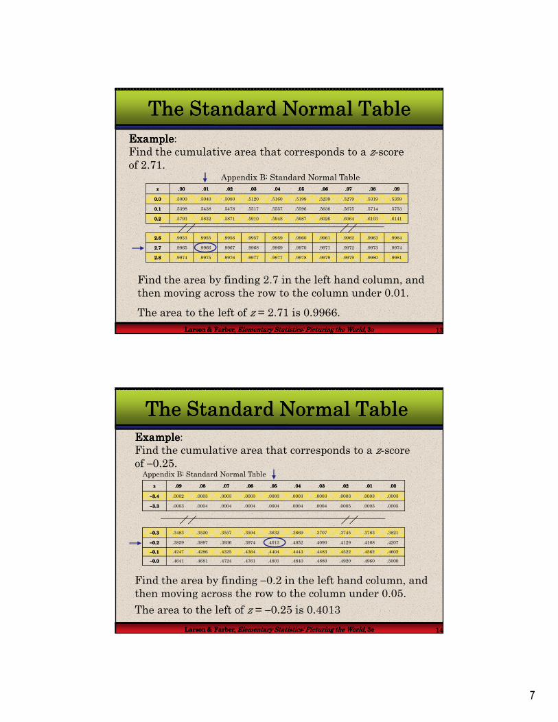
The Standard Normal TableThe Standard Normal TableThe Standard Normal TableThe Standard Normal Table
ExampleExampleExampleExample:
Find the cumulative area that corresponds to a z-score of 2.71.
z z z z ....00 00 00 00 ....01 01 01 01 ....02 02 02 02 ....03 03 03 03 ....04 04 04 04 ....05 05 05 05 ....06 06 06 06 ....07 07 07 07 ....08 08 08 08 ....09 09 09 09
0000....0 0 0 0 .5000 .5040 .5080 .5120 .5160 .5199 .5239 .5279 .5319 .5359
0000....1 1 1 1 .5398 .5438 .5478 .5517 .5557 .5596 .5636 .5675 .5714 .5753
0000....2 2 2 2 .5793 .5832 .5871 .5910 .5948 .5987 .6026 .6064 .6103 .6141
2222....6 6 6 6 .9953 .9955 .9956 .9957 .9959 .9960 .9961 .9962 .9963 .9964
2222....7 7 7 7 .9965 .9966 .9967 .9968 .9969 .9970 .9971 .9972 .9973 .9974
2222....8 8 8 8 .9974 .9975 .9976 .9977 .9977 .9978 .9979 .9979 .9980 .9981
Find the area by finding 2.7 in the left hand column, and then moving across the row to the column under 0.01.
The area to the left of z = 2.71 is 0.9966.
Appendix B: Standard Normal Table
Larson & Farber, Larson & Farber, Larson & Farber, Larson & Farber, Elementary Statistics: Picturing the WorldElementary Statistics: Picturing the WorldElementary Statistics: Picturing the WorldElementary Statistics: Picturing the World, , , , 3333eeee 14141414
The Standard Normal TableThe Standard Normal TableThe Standard Normal TableThe Standard Normal TableExampleExampleExampleExample:
Find the cumulative area that corresponds to a z-score of −0.25.
z z z z ....09 09 09 09 ....08 08 08 08 ....07070707 ....06060606 ....05050505 ....04040404 ....03030303 ....02020202 ....01010101 ....00000000
−−−−3333....4444 .0002 .0003 .0003 .0003 .0003 .0003 .0003 .0003 .0003 .0003
−−−−3333....3333 .0003 .0004 .0004 .0004 .0004 .0004 .0004 .0005 .0005 .0005
Find the area by finding −0.2 in the left hand column, and then moving across the row to the column under 0.05.
The area to the left of z = −0.25 is 0.4013
−−−−0000....3 3 3 3 .3483 .3520 .3557 .3594 .3632 .3669 .3707 .3745 .3783 .3821
−−−−0000....2222 .3859 .3897 .3936 .3974 .4013 .4052 .4090 .4129 .4168 .4207
−−−−0000....1111 .4247 .4286 .4325 .4364 .4404 .4443 .4483 .4522 .4562 .4602
−−−−0000....0000 .4641 .4681 .4724 .4761 .4801 .4840 .4880 .4920 .4960 .5000
Appendix B: Standard Normal Table

8
Larson & Farber, Larson & Farber, Larson & Farber, Larson & Farber, Elementary Statistics: Picturing the WorldElementary Statistics: Picturing the WorldElementary Statistics: Picturing the WorldElementary Statistics: Picturing the World, , , , 3333eeee 15151515
Guidelines for Finding AreasGuidelines for Finding AreasGuidelines for Finding AreasGuidelines for Finding Areas
Finding Areas Under the Standard Normal CurveFinding Areas Under the Standard Normal CurveFinding Areas Under the Standard Normal CurveFinding Areas Under the Standard Normal Curve1. Sketch the standard normal curve and shade the
appropriate area under the curve.
2. Find the area by following the directions for each case shown.
a. To find the area to the left of z, find the area that corresponds to z in the Standard Normal Table.
1. Use the table to find the area for the z-score.
2. The area to the left of z = 1.23 is 0.8907.
1.230
z
Larson & Farber, Larson & Farber, Larson & Farber, Larson & Farber, Elementary Statistics: Picturing the WorldElementary Statistics: Picturing the WorldElementary Statistics: Picturing the WorldElementary Statistics: Picturing the World, , , , 3333eeee 16161616
Guidelines for Finding AreasGuidelines for Finding AreasGuidelines for Finding AreasGuidelines for Finding Areas
Finding Areas Under the Standard Normal CurveFinding Areas Under the Standard Normal CurveFinding Areas Under the Standard Normal CurveFinding Areas Under the Standard Normal Curve
b. To find the area to the right of z, use the Standard Normal Table to find the area that corresponds to z. Then subtract the area from 1.
3. Subtract to find the area to the right of z = 1.23:1 − 0.8907 = 0.1093.
1. Use the table to find the area for the z-score.
2. The area to the left of z = 1.23 is 0.8907.
1.230
z

9
Larson & Farber, Larson & Farber, Larson & Farber, Larson & Farber, Elementary Statistics: Picturing the WorldElementary Statistics: Picturing the WorldElementary Statistics: Picturing the WorldElementary Statistics: Picturing the World, , , , 3333eeee 17171717
Finding Areas Under the Standard Normal CurveFinding Areas Under the Standard Normal CurveFinding Areas Under the Standard Normal CurveFinding Areas Under the Standard Normal Curvec. To find the area between two z-scores, find the area
corresponding to each z-score in the Standard Normal Table. Then subtract the smaller area from the larger area.
Guidelines for Finding AreasGuidelines for Finding AreasGuidelines for Finding AreasGuidelines for Finding Areas
4. Subtract to find the area of the region between the two z-scores: 0.8907 − 0.2266 = 0.6641.
1. Use the table to find the area for the z-score.
3. The area to the left of z = −0.75 is 0.2266.
2. The area to the left of z = 1.23 is 0.8907.
1.230
z
−0.75
Larson & Farber, Larson & Farber, Larson & Farber, Larson & Farber, Elementary Statistics: Picturing the WorldElementary Statistics: Picturing the WorldElementary Statistics: Picturing the WorldElementary Statistics: Picturing the World, , , , 3333eeee 18181818
Guidelines for Finding AreasGuidelines for Finding AreasGuidelines for Finding AreasGuidelines for Finding Areas
ExampleExampleExampleExample:
Find the area under the standard normal curve to the left of z = −2.33.
From the Standard Normal Table, the area is equal to 0.0099.
Always draw the curve!
−2.33 0
z

10
Larson & Farber, Larson & Farber, Larson & Farber, Larson & Farber, Elementary Statistics: Picturing the WorldElementary Statistics: Picturing the WorldElementary Statistics: Picturing the WorldElementary Statistics: Picturing the World, , , , 3333eeee 19191919
Guidelines for Finding AreasGuidelines for Finding AreasGuidelines for Finding AreasGuidelines for Finding Areas
ExampleExampleExampleExample:
Find the area under the standard normal curve to the right of z = 0.94.
From the Standard Normal Table, the area is equal to 0.1736.
Always draw the curve!
0.82641 − 0.8264 = 0.1736
0.940
z
Larson & Farber, Larson & Farber, Larson & Farber, Larson & Farber, Elementary Statistics: Picturing the WorldElementary Statistics: Picturing the WorldElementary Statistics: Picturing the WorldElementary Statistics: Picturing the World, , , , 3333eeee 20202020
Guidelines for Finding AreasGuidelines for Finding AreasGuidelines for Finding AreasGuidelines for Finding Areas
ExampleExampleExampleExample:
Find the area under the standard normal curve between z = −1.98 and z = 1.07.
From the Standard Normal Table, the area is equal to 0.8338.
Always draw the curve!
0.8577 − 0.0239 = 0.8338
0.8577
0.0239
1.070
z
−1.98
11
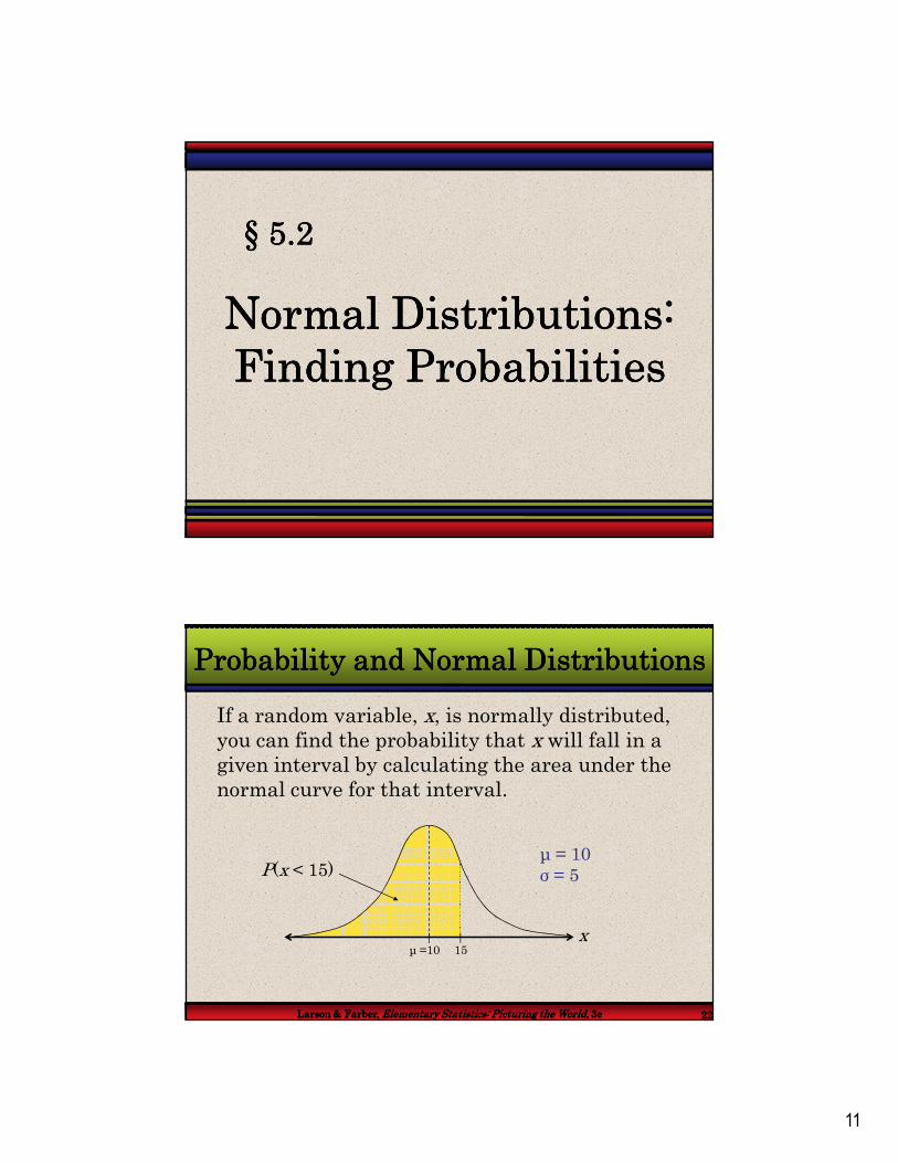
§§§§ 5555....2222
Normal Distributions: Normal Distributions: Normal Distributions: Normal Distributions: Finding ProbabilitiesFinding ProbabilitiesFinding ProbabilitiesFinding Probabilities
Larson & Farber, Larson & Farber, Larson & Farber, Larson & Farber, Elementary Statistics:Elementary Statistics:Elementary Statistics:Elementary Statistics: Picturing the WorldPicturing the WorldPicturing the WorldPicturing the World, , , , 3333eeee 22222222
Probability and Normal DistributionsProbability and Normal DistributionsProbability and Normal DistributionsProbability and Normal Distributions
If a random variable, x, is normally distributed, you can find the probability that x will fall in a given interval by calculating the area under the normal curve for that interval.
P(x < 15)µ = 10σ = 5
15µ =10x

12
Larson & Farber, Larson & Farber, Larson & Farber, Larson & Farber, Elementary Statistics: Picturing the WorldElementary Statistics: Picturing the WorldElementary Statistics: Picturing the WorldElementary Statistics: Picturing the World, , , , 3333eeee 23232323
Probability and Normal DistributionsProbability and Normal DistributionsProbability and Normal DistributionsProbability and Normal Distributions
Same area
P(x < 15) = P(z < 1) = Shaded area under the curve
= 0.8413
15µ =10
P(x < 15)
µ = 10σ = 5
Normal Distribution
x1µ =0
µ = 0σ = 1
Standard Normal Distribution
z
P(z < 1)
Larson & Farber, Larson & Farber, Larson & Farber, Larson & Farber, Elementary Statistics: Picturing the WorldElementary Statistics: Picturing the WorldElementary Statistics: Picturing the WorldElementary Statistics: Picturing the World, , , , 3333eeee 24242424
ExampleExampleExampleExample:
The average on a statistics test was 78 with a standard deviation of 8. If the test scores are normally distributed, find the probability that a student receives a test score less than 90.
Probability and Normal DistributionsProbability and Normal DistributionsProbability and Normal DistributionsProbability and Normal Distributions
P(x < 90) = P(z < 1.5) = 0.9332
-=
90 -78=
8x µz
σ= 1.5
The probability that a student receives a test score less than 90 is 0.9332.
µ =0z
?1111....5555
90µ =78
P(x < 90)
µ = 78σ = 8
x

13
Larson & Farber, Larson & Farber, Larson & Farber, Larson & Farber, Elementary Statistics: Picturing the WorldElementary Statistics: Picturing the WorldElementary Statistics: Picturing the WorldElementary Statistics: Picturing the World, , , , 3333eeee 25252525
ExampleExampleExampleExample:
The average on a statistics test was 78 with a standard deviation of 8. If the test scores are normally distributed, find the probability that a student receives a test score greater than than 85.
Probability and Normal DistributionsProbability and Normal DistributionsProbability and Normal DistributionsProbability and Normal Distributions
P(x > 85) = P(z > 0.88) = 1 − P(z < 0.88) = 1 − 0.8106 = 0.1894
85-78= =
8x - µz
σ≈= 0.875 0.88
The probability that a student receives a test score greater than 85 is 0.1894.
µ =0z
?0000....88888888
85µ =78
P(x > 85)
µ = 78σ = 8
x
Larson & Farber, Larson & Farber, Larson & Farber, Larson & Farber, Elementary Statistics: Picturing the WorldElementary Statistics: Picturing the WorldElementary Statistics: Picturing the WorldElementary Statistics: Picturing the World, , , , 3333eeee 26262626
ExampleExampleExampleExample:
The average on a statistics test was 78 with a standard deviation of 8. If the test scores are normally distributed, find the probability that a student receives a test score between 60 and 80.
Probability and Normal DistributionsProbability and Normal DistributionsProbability and Normal DistributionsProbability and Normal Distributions
P(60 < x < 80) = P(−2.25 < z < 0.25) = P(z < 0.25) − P(z < −2.25)
- -1
60 78= =
8x µz
σ-= 2.25
The probability that a student receives a test score between 60 and 80 is 0.5865.
2
- -=
80 78=
8x µz
σ= 0.25
µ =0z
?? 0.25−2.25
= 0.5987 − 0.0122 = 0.5865
60 80µ =78
P(60 < x < 80)
µ = 78σ = 8
x

14
§§§§ 5555....3333
Normal Distributions: Normal Distributions: Normal Distributions: Normal Distributions: Finding ValuesFinding ValuesFinding ValuesFinding Values
Larson & Farber, Larson & Farber, Larson & Farber, Larson & Farber, Elementary Statistics:Elementary Statistics:Elementary Statistics:Elementary Statistics: Picturing the WorldPicturing the WorldPicturing the WorldPicturing the World, , , , 3333eeee 28282828
Finding zFinding zFinding zFinding z----ScoresScoresScoresScores
ExampleExampleExampleExample:
Find the z-score that corresponds to a cumulative area of 0.9973.
z z z z ....00 00 00 00 ....01 01 01 01 ....02 02 02 02 ....03 03 03 03 ....04 04 04 04 ....05 05 05 05 ....06 06 06 06 ....07 07 07 07 ....08 08 08 08 ....09 09 09 09
0000....0 0 0 0 .5000 .5040 .5080 .5120 .5160 .5199 .5239 .5279 .5319 .5359
0000....1 1 1 1 .5398 .5438 .5478 .5517 .5557 .5596 .5636 .5675 .5714 .5753
0000....2 2 2 2 .5793 .5832 .5871 .5910 .5948 .5987 .6026 .6064 .6103 .6141
2222....6 6 6 6 .9953 .9955 .9956 .9957 .9959 .9960 .9961 .9962 .9963 .9964
2222....7 7 7 7 .9965 .9966 .9967 .9968 .9969 .9970 .9971 .9972 .9973 .9974
2222....8 8 8 8 .9974 .9975 .9976 .9977 .9977 .9978 .9979 .9979 .9980 .9981
Find the z-score by locating 0.9973 in the body of the Standard Normal Table. The values at the beginning of the corresponding row and at the top of the column give the z-score.
The z-score is 2.78.
Appendix B: Standard Normal Table
2222....7777
....08080808

15
Larson & Farber, Larson & Farber, Larson & Farber, Larson & Farber, Elementary Statistics: Picturing the WorldElementary Statistics: Picturing the WorldElementary Statistics: Picturing the WorldElementary Statistics: Picturing the World, , , , 3333eeee 29292929
Finding zFinding zFinding zFinding z----ScoresScoresScoresScores
ExampleExampleExampleExample:
Find the z-score that corresponds to a cumulative area of 0.4170.
z z z z ....09 09 09 09 ....08 08 08 08 ....07070707 ....06060606 ....05050505 ....04040404 ....03030303 ....02020202 ....01010101 ....00000000
−−−−3333....4444 .0002 .0003 .0003 .0003 .0003 .0003 .0003 .0003 .0003 .0003
−−−−0000....2222 .0003 .0004 .0004 .0004 .0004 .0004 .0004 .0005 .0005 .0005
Find the z-score by locating 0.4170 in the body of the Standard Normal Table. Use the value closest to 0.4170.
−−−−0000....3 3 3 3 .3483 .3520 .3557 .3594 .3632 .3669 .3707 .3745 .3783 .3821
−−−−0000....2222 .3859 .3897 .3936 .3974 .4013 .4052 .4090 .4129 .4168 .4207
−−−−0000....1111 .4247 .4286 .4325 .4364 .4404 .4443 .4483 .4522 .4562 .4602
−−−−0000....0000 .4641 .4681 .4724 .4761 .4801 .4840 .4880 .4920 .4960 .5000
Appendix B: Standard Normal Table
Use the closest area.
The z-score is −0.21.
−−−−0000....2222
....01010101
Larson & Farber, Larson & Farber, Larson & Farber, Larson & Farber, Elementary Statistics: Picturing the WorldElementary Statistics: Picturing the WorldElementary Statistics: Picturing the WorldElementary Statistics: Picturing the World, , , , 3333eeee 30303030
Finding a zFinding a zFinding a zFinding a z----Score Given a PercentileScore Given a PercentileScore Given a PercentileScore Given a Percentile
ExampleExampleExampleExample:
Find the z-score that corresponds to P75.
The z-score that corresponds to P75 is the same z-score that corresponds to an area of 0.75.
The z-score is 0.67.
?µ =0z
0.67
Area = 0.75
16
Larson & Farber, Larson & Farber, Larson & Farber, Larson & Farber, Elementary Statistics: Picturing the WorldElementary Statistics: Picturing the WorldElementary Statistics: Picturing the WorldElementary Statistics: Picturing the World, , , , 3333eeee 31313131
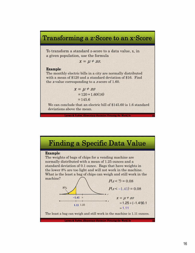
Transforming a zTransforming a zTransforming a zTransforming a z----Score to an xScore to an xScore to an xScore to an x----ScoreScoreScoreScore
To transform a standard z-score to a data value, x, in a given population, use the formula
ExampleExampleExampleExample:
The monthly electric bills in a city are normally distributed with a mean of $120 and a standard deviation of $16. Find the x-value corresponding to a z-score of 1.60.
=x µ + zσ.
=x µ + zσ= 120 +1.60(16)
= 145.6
We can conclude that an electric bill of $145.60 is 1.6 standard deviations above the mean.
Larson & Farber, Larson & Farber, Larson & Farber, Larson & Farber, Elementary Statistics:Elementary Statistics:Elementary Statistics:Elementary Statistics: Picturing the WorldPicturing the WorldPicturing the WorldPicturing the World, , , , 3333eeee 32323232
Finding a Specific Data ValueFinding a Specific Data ValueFinding a Specific Data ValueFinding a Specific Data ValueExampleExampleExampleExample:
The weights of bags of chips for a vending machine are normally distributed with a mean of 1.25 ounces and a standard deviation of 0.1 ounce. Bags that have weights in the lower 8% are too light and will not work in the machine. What is the least a bag of chips can weigh and still work in the machine?
=x µ + zσ
The least a bag can weigh and still work in the machine is 1.11 ounces.
? 0
z
8%
P(z < ?) = 0.08
P(z < −1.41) = 0.08
−−−−1111....41414141
1.25
x
?1.25 ( 1.41)0.1= + −
= 1.111111....11111111

17
§§§§ 5555....4444
Sampling Distributions Sampling Distributions Sampling Distributions Sampling Distributions and the Central Limit and the Central Limit and the Central Limit and the Central Limit
TheoremTheoremTheoremTheorem
Larson & Farber, Larson & Farber, Larson & Farber, Larson & Farber, Elementary Statistics:Elementary Statistics:Elementary Statistics:Elementary Statistics: Picturing the WorldPicturing the WorldPicturing the WorldPicturing the World, , , , 3333eeee 34343434
PopulationPopulationPopulationPopulation
Sample
Sampling DistributionsSampling DistributionsSampling DistributionsSampling Distributions
A sampling distributionsampling distributionsampling distributionsampling distribution is the probability distribution of a sample statistic that is formed when samples of size n are repeatedly taken from a population.
Sample
Sample
Sample Sample
Sample
Sample
Sample
Sample
Sample

18
Larson & Farber, Larson & Farber, Larson & Farber, Larson & Farber, Elementary Statistics: Picturing the WorldElementary Statistics: Picturing the WorldElementary Statistics: Picturing the WorldElementary Statistics: Picturing the World, , , , 3333eeee 35353535
Sampling DistributionsSampling DistributionsSampling DistributionsSampling Distributions
If the sample statistic is the sample mean, then the distribution is the sampling distribution of sample meanssampling distribution of sample meanssampling distribution of sample meanssampling distribution of sample means.
Sample 1
1xSample 4
4x
Sample 3
3x Sample 6
6x
The sampling distribution consists of the values of the
sample means, 1 2 3 4 5 6, , , , , . x x x x x x
Sample 2
2xSample 5
5x
Larson & Farber, Larson & Farber, Larson & Farber, Larson & Farber, Elementary Statistics:Elementary Statistics:Elementary Statistics:Elementary Statistics: Picturing the WorldPicturing the WorldPicturing the WorldPicturing the World, , , , 3333eeee 36363636
Properties of Sampling DistributionsProperties of Sampling DistributionsProperties of Sampling DistributionsProperties of Sampling Distributions
Properties of Sampling Distributions of Sample MeansProperties of Sampling Distributions of Sample MeansProperties of Sampling Distributions of Sample MeansProperties of Sampling Distributions of Sample Means
1. The mean of the sample means, is equal to the population
mean.
2. The standard deviation of the sample means, is equal to the
population standard deviation, divided by the square root of n.
The standard deviation of the sampling distribution of the sample
means is called the standard error of thestandard error of thestandard error of thestandard error of the meanmeanmeanmean.
,xµ
xµ = µ
,xσ
,σ
xσσ =n

19
Larson & Farber, Larson & Farber, Larson & Farber, Larson & Farber, Elementary Statistics:Elementary Statistics:Elementary Statistics:Elementary Statistics: Picturing the WorldPicturing the WorldPicturing the WorldPicturing the World, , , , 3333eeee 37373737
Sampling Distribution of Sample MeansSampling Distribution of Sample MeansSampling Distribution of Sample MeansSampling Distribution of Sample Means
ExampleExampleExampleExample:
The population values {5, 10, 15, 20} are written on slips of paper and put in a hat. Two slips are randomly selected, with replacement.
a. Find the mean, standard deviation, and variance of the population.
Continued.
= 12.5µ
= 5.59σ
2 = 31.25σ
PopulationPopulationPopulationPopulation5
101520
Larson & Farber, Larson & Farber, Larson & Farber, Larson & Farber, Elementary Statistics:Elementary Statistics:Elementary Statistics:Elementary Statistics: Picturing the WorldPicturing the WorldPicturing the WorldPicturing the World, , , , 3333eeee 38383838
Sampling Distribution of Sample MeansSampling Distribution of Sample MeansSampling Distribution of Sample MeansSampling Distribution of Sample Means
Example continuedExample continuedExample continuedExample continued:
The population values {5, 10, 15, 20} are written on slips of paper and put in a hat. Two slips are randomly selected, with replacement.
b. Graph the probability histogram for the population values.
Continued.
This uniform distribution shows that all values have the same probability of being selected.
Population values
Pro
babil
ity
0.25
5 10 15 20
x
P(x) Probability Histogram Probability Histogram Probability Histogram Probability Histogram of Population of of Population of of Population of of Population of xxxx
20
Larson & Farber, Larson & Farber, Larson & Farber, Larson & Farber, Elementary Statistics: Picturing the WorldElementary Statistics: Picturing the WorldElementary Statistics: Picturing the WorldElementary Statistics: Picturing the World, , , , 3333eeee 39393939
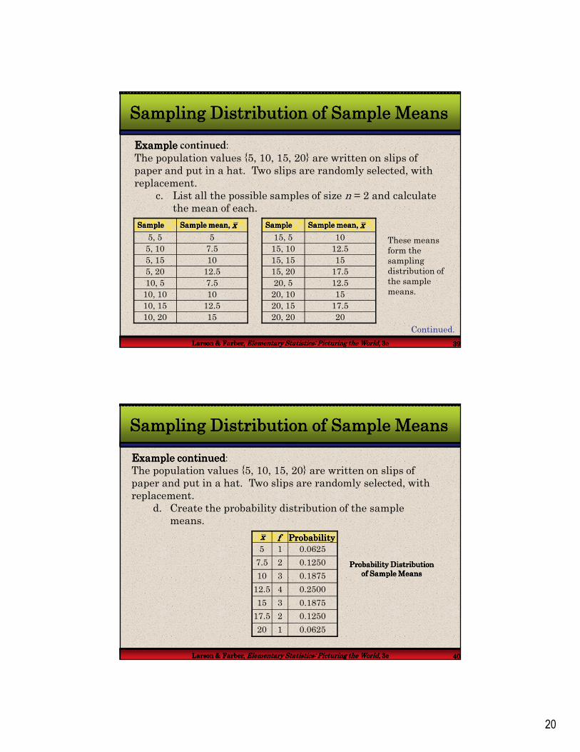
Sampling Distribution of Sample MeansSampling Distribution of Sample MeansSampling Distribution of Sample MeansSampling Distribution of Sample Means
Example Example Example Example continued:
The population values {5, 10, 15, 20} are written on slips of paper and put in a hat. Two slips are randomly selected, with replacement.
c. List all the possible samples of size n = 2 and calculate the mean of each.
1510, 20
12.510, 15
1010, 10
7.510, 5
12.55, 20
105, 15
7.55, 10
55, 5
Sample mean, Sample mean, Sample mean, Sample mean, SampleSampleSampleSample xxxx
2020, 20
17.520, 15
1520, 10
12.520, 5
17.515, 20
1515, 15
12.515, 10
1015, 5
Sample mean, Sample mean, Sample mean, Sample mean, SampleSampleSampleSample xxxx
Continued.
These means form the sampling distribution of the sample means.
Larson & Farber, Larson & Farber, Larson & Farber, Larson & Farber, Elementary Statistics: Picturing the WorldElementary Statistics: Picturing the WorldElementary Statistics: Picturing the WorldElementary Statistics: Picturing the World, , , , 3333eeee 40404040
Sampling Distribution of Sample MeansSampling Distribution of Sample MeansSampling Distribution of Sample MeansSampling Distribution of Sample Means
Example continuedExample continuedExample continuedExample continued:
The population values {5, 10, 15, 20} are written on slips of paper and put in a hat. Two slips are randomly selected, with replacement.
d. Create the probability distribution of the sample means.
Probability Distribution Probability Distribution Probability Distribution Probability Distribution of Sample Meansof Sample Meansof Sample Meansof Sample Means
0.0625120
0.1250217.5
0.1875315
0.2500412.5
0.1875310
0.125027.5
0.062515
xxxx ffff ProbabilityProbabilityProbabilityProbability

21
Larson & Farber, Larson & Farber, Larson & Farber, Larson & Farber, Elementary Statistics: Picturing the WorldElementary Statistics: Picturing the WorldElementary Statistics: Picturing the WorldElementary Statistics: Picturing the World, , , , 3333eeee 41414141
Sampling Distribution of Sample MeansSampling Distribution of Sample MeansSampling Distribution of Sample MeansSampling Distribution of Sample Means
Example continuedExample continuedExample continuedExample continued:
The population values {5, 10, 15, 20} are written on slips of paper and put in a hat. Two slips are randomly selected, with replacement.
e. Graph the probability histogram for the sampling distribution.
The shape of the graph is symmetric and bell shaped. It approximates a normal distribution.
Sample mean
Pro
babil
ity
0.25
P(x) Probability Histogram of Probability Histogram of Probability Histogram of Probability Histogram of Sampling DistributionSampling DistributionSampling DistributionSampling Distribution
0.20
0.15
0.10
0.05
17.5 201512.5107.55
x
Larson & Farber, Larson & Farber, Larson & Farber, Larson & Farber, Elementary Statistics: Picturing the WorldElementary Statistics: Picturing the WorldElementary Statistics: Picturing the WorldElementary Statistics: Picturing the World, , , , 3333eeee 42424242
the sample meanssample meanssample meanssample means will have a normal distributionnormal distributionnormal distributionnormal distribution.
The Central Limit TheoremThe Central Limit TheoremThe Central Limit TheoremThe Central Limit Theorem
If a sample of size n ≥ 30 is taken from a population with any type ofany type ofany type ofany type of distributiondistributiondistributiondistribution that has a mean = µ and standard deviation = σ,
xµ
xµ
µ
x
x
x
x
x
xxxx
x
x
xx

22
Larson & Farber, Larson & Farber, Larson & Farber, Larson & Farber, Elementary Statistics:Elementary Statistics:Elementary Statistics:Elementary Statistics: Picturing the WorldPicturing the WorldPicturing the WorldPicturing the World, , , , 3333eeee 43434343
The Central Limit TheoremThe Central Limit TheoremThe Central Limit TheoremThe Central Limit Theorem
If the population itself is normally distributednormally distributednormally distributednormally distributed, with mean = µ and standard deviation = σ,
the sample meanssample meanssample meanssample means will have a normal distributionnormal distributionnormal distributionnormal distribution for any sample size n.
µx
µ
x
x
x
x
x
xxxx
x
x
xx
Larson & Farber, Larson & Farber, Larson & Farber, Larson & Farber, Elementary Statistics: Picturing the WorldElementary Statistics: Picturing the WorldElementary Statistics: Picturing the WorldElementary Statistics: Picturing the World, , , , 3333eeee 44444444
The Central Limit TheoremThe Central Limit TheoremThe Central Limit TheoremThe Central Limit Theorem
In either case, the sampling distribution of sample means has a mean equal to the population mean.
=xµ µ
=xσσn
Mean of the sample means
Standard deviation of the sample means
The sampling distribution of sample means has a standard deviation equal to the population standard deviation divided by the square root of n.
This is also called the standard error of the meanstandard error of the meanstandard error of the meanstandard error of the mean.

23
Larson & Farber, Larson & Farber, Larson & Farber, Larson & Farber, Elementary Statistics:Elementary Statistics:Elementary Statistics:Elementary Statistics: Picturing the WorldPicturing the WorldPicturing the WorldPicturing the World, , , , 3333eeee 45454545
The Mean and Standard ErrorThe Mean and Standard ErrorThe Mean and Standard ErrorThe Mean and Standard Error
ExampleExampleExampleExample:
The heights of fully grown magnolia bushes have a mean height of 8 feet and a standard deviation of 0.7 feet. 38 bushes are randomly selected from the population, and the mean of each sample is determined. Find the mean and standard error of the mean of the sampling distribution.
=xµ µMeanMeanMeanMean
Standard deviation Standard deviation Standard deviation Standard deviation (standard error)(standard error)(standard error)(standard error)
=x
σσn
= 80.7
=38
= 0.11
Continued.
Larson & Farber, Larson & Farber, Larson & Farber, Larson & Farber, Elementary Statistics:Elementary Statistics:Elementary Statistics:Elementary Statistics: Picturing the WorldPicturing the WorldPicturing the WorldPicturing the World, , , , 3333eeee 46464646
Interpreting the Central Limit TheoremInterpreting the Central Limit TheoremInterpreting the Central Limit TheoremInterpreting the Central Limit Theorem
Example continuedExample continuedExample continuedExample continued:
The heights of fully grown magnolia bushes have a mean height of 8 feet and a standard deviation of 0.7 feet. 38 bushes are randomly selected from the population, and the mean of each sample is determined.
From the Central Limit Theorem, because the sample size is greater than 30, the sampling distribution can be approximated by the normal distribution.
The mean of the sampling distribution is 8 feet ,and the standard error of the sampling distribution is 0.11 feet.
x
8 8.47.6
= 8xµ = 0.11xσ

24
Larson & Farber, Larson & Farber, Larson & Farber, Larson & Farber, Elementary Statistics: Picturing the WorldElementary Statistics: Picturing the WorldElementary Statistics: Picturing the WorldElementary Statistics: Picturing the World, , , , 3333eeee 47474747
Finding ProbabilitiesFinding ProbabilitiesFinding ProbabilitiesFinding Probabilities
ExampleExampleExampleExample:
The heights of fully grown magnolia bushes have a mean height of 8 feet and a standard deviation of 0.7 feet. 38 bushes are randomly selected from the population, and the mean of each sample is determined.
Find the probability that the mean height of the 38 bushes is less than 7.8 feet.
The mean of the sampling distribution is 8 feet, and the standard error of the sampling distribution is 0.11 feet.
7.8
x
8.47.6 8
Continued.
=8xµ
=0.11xσ=38n
Larson & Farber, Larson & Farber, Larson & Farber, Larson & Farber, Elementary Statistics: Picturing the WorldElementary Statistics: Picturing the WorldElementary Statistics: Picturing the WorldElementary Statistics: Picturing the World, , , , 3333eeee 48484848
P ( < 7.8) = P (z < ____ )????x −−−−1111....82828282
Finding ProbabilitiesFinding ProbabilitiesFinding ProbabilitiesFinding Probabilities
Example continuedExample continuedExample continuedExample continued:
Find the probability that the mean height of the 38 bushes is less than 7.8 feet.
−= x
x
x µz
σ
−7.8 8=0.117.8
x
8.47.6 8
= 8xµ
= 0.11xσn = 38
−= 1.82
z
0
The probability that the mean height of the 38 bushes is less than 7.8 feet is 0.0344.
= 0.0344
P ( < 7.8)x

25
Larson & Farber, Larson & Farber, Larson & Farber, Larson & Farber, Elementary Statistics: Picturing the WorldElementary Statistics: Picturing the WorldElementary Statistics: Picturing the WorldElementary Statistics: Picturing the World, , , , 3333eeee 49494949
ExampleExampleExampleExample:
The average on a statistics test was 78 with a standard deviation of 8. If the test scores are normally distributed, find the probability that the mean score of 25 randomly selected students is between 75 and 79.
Probability and Normal DistributionsProbability and Normal DistributionsProbability and Normal DistributionsProbability and Normal Distributions
− −x
x
x µz
σ1
75 78= =
1.6−= 1.88
− −x µzσ2
79 78= =
1.6= 0.63
0z
?? 0.63−1.88
= 78
σ 8= = = 1.6
n 25
x
x
µ
σ
Continued.
P (75 < < 79)x
75 7978x
Larson & Farber, Larson & Farber, Larson & Farber, Larson & Farber, Elementary Statistics: Picturing the WorldElementary Statistics: Picturing the WorldElementary Statistics: Picturing the WorldElementary Statistics: Picturing the World, , , , 3333eeee 50505050
Example continuedExample continuedExample continuedExample continued:
Probability and Normal DistributionsProbability and Normal DistributionsProbability and Normal DistributionsProbability and Normal Distributions
Approximately 70.56% of the 25 students will have a mean score between 75 and 79.
= 0.7357 − 0.0301 = 0.7056
0z
?? 0.63−1.88
P (75 < < 79)x
P(75 < < 79) = P(−1.88 < z < 0.63) = P(z < 0.63) − P(z < −1.88) x
75 7978x
26
Larson & Farber, Larson & Farber, Larson & Farber, Larson & Farber, Elementary Statistics: Picturing the WorldElementary Statistics: Picturing the WorldElementary Statistics: Picturing the WorldElementary Statistics: Picturing the World, , , , 3333eeee 51515151
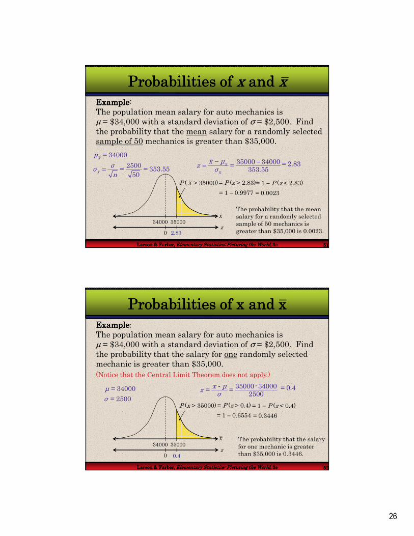
ExampleExampleExampleExample:The population mean salary for auto mechanics is µ = $34,000 with a standard deviation of σ = $2,500. Find the probability that the mean salary for a randomly selected sample of 50 mechanics is greater than $35,000.
Probabilities of Probabilities of Probabilities of Probabilities of xxxx and and and and xxxx
− −= x
x
x µz
σ35000 34000
=353.55
= 2.83
0z
?2.83
=
= 34000
2500= = 353.55
50
x
x
µ
σσn
= P (z > 2.83)= 1 − P (z < 2.83)
= 1 − 0.9977 = 0.0023
The probability that the mean salary for a randomly selected sample of 50 mechanics is greater than $35,000 is 0.0023.
3500034000
P ( > 35000)x
x
Larson & Farber, Larson & Farber, Larson & Farber, Larson & Farber, Elementary Statistics: Picturing the WorldElementary Statistics: Picturing the WorldElementary Statistics: Picturing the WorldElementary Statistics: Picturing the World, , , , 3333eeee 52525252
ExampleExampleExampleExample:
The population mean salary for auto mechanics is µ = $34,000 with a standard deviation of σ = $2,500. Find the probability that the salary for one randomly selected mechanic is greater than $35,000.
Probabilities of x and x Probabilities of x and x Probabilities of x and x Probabilities of x and x
- 35000-34000= =
2500x µz
σ= 0.4
0z
?0.4
= 34000
= 2500
µ
σ= P (z > 0.4) = 1 − P (z < 0.4)
= 1 − 0.6554 = 0.3446
The probability that the salary for one mechanic is greater than $35,000 is 0.3446.
(Notice that the Central Limit Theorem does not apply.)
3500034000
P (x > 35000)
x

27
Larson & Farber, Larson & Farber, Larson & Farber, Larson & Farber, Elementary Statistics: Picturing the WorldElementary Statistics: Picturing the WorldElementary Statistics: Picturing the WorldElementary Statistics: Picturing the World, , , , 3333eeee 53535353
ExampleExampleExampleExample:
The probability that the salary for one randomly selected mechanic is greater than $35,000 is 0.3446. In a group of 50 mechanics, approximately how many would have a salary greater than $35,000?
Probabilities of Probabilities of Probabilities of Probabilities of xxxx and and and and xxxx
P(x > 35000) = 0.3446This also means that 34.46% of mechanics have a salary greater than $35,000.
You would expect about 17 mechanics out of the group of 50 to have a salary greater than $35,000.
34.46% of 50 = 0.3446 × 50 = 17.23