chapter five study of behaviour of equity returns analysis...

Chapter Five

STUDY OF BEHAVIOUR OF EQUITY RETURNSANALYSIS I

Chapter Five

STUDY OF BEHAVIOUR OF EQUITY RETURNSANALYSIS I

In this chapter, the behavior of all the 20 stocks under study wasexamined in detail. The equity return behavior of the stocks was studied interms of the stocks’ daily returns, average annual returns and Holding PeriodYield. The volatility in returns was given paramount importance in thestudy. The daily returns of the individual stocks for 10 year period from1999 to 2009 were examined to understand their behavior. The statisticaltools like Arithmetic mean, standard deviation, measure of skewness,kurtosis, variances and all were used to study the daily and annual returns.Annual returns were averaged by the number of actual market working daysfor the relevant year. The arithmetic average returns of every year for the tenyears were studied for establishing the behavior. Similarly, Holding PeriodYields of the scrips were worked from the daily returns on yearly basis forall the 10 years to study their behavior. The returns were:

1. Daily Returns (DR)2. Annual Returns (AR)3. Holding Period Yield (HPY)

The returns were calculated as given

1. Daily returns

DR = − 1 100

Here,

P1= New priceP0 = Previous day’s price

2. Annual Returns

=

3. Holding Period Yield (HPY)

HPY =( )-1=( − 1)100

Here,

P1 = Closing Stock price of the yearP0 = Opening stock price of the year

In the analysis, a detailed summary statistics were calculated andgiven as table. The summary statistics includes,

1. Arithmetic mean2. Standard deviation(σ)3. variance(σ2)4. co-variance(Cov)5. skewness6. kurtosis7. correlation(r)8. beta coefficient9. R2 value.

They were all used to analyse the behavior of returns supplementedby tables and graphs.An individual company-wise study of thebehavior of equity returns were carried out on the above backdropas below:

1. ACC

Table No.5.1Summary statistics of ACC from 1999 to 2009

Source: Official website of Bombay Stock Exchange

As per Table 1, the average return of ACC for the period from 1999 to2009 was 0.09%. But the estimated return as represented by the holdingperiod yield (HPY) for the same period was 13.5%. It could be seen that thescrip’s performance was much below the estimated. Similarly ACC’saverage return was lower than the market return of 0.11%. The standarddeviation and variance were slightly significant. During the 10 year periodthe return went up to 15.6% and went down to the extent of -91.84%.

The σ 3.32 and the var.11.04 signify volatility in the return. The rangeof return between the prosperity and adversity 108 was also significant andshows exceptional volatility. The distribution was negatively skewed to theextent of -7.61 which is statistically significant. The value of kurtosis isbigger than 3. The distribution is high leptokurtic.

The correlation between ACC and BSEI were 0.025. It is highlyinsignificant. But both move to the same direction positively. There is only aslight covariance between them to the extent of 0.149. The beta value is lessthan one. The risk of the scrip is considerably lower than the marketportfolio. R2 value is only 0.0006 which says that only an infinitesimal partof the variance is explained by the market and the remaining 99% of thevariance was unexplained by the market.

Average return 0.09% Skewness -7.61σ 3.32 Variance 11.04L 15.6 Cov. 0.15S -91.84 kurtosis 212.01Range 108 cor. 0.025Beta 0.046R2 0.0006 HPY 13.5%

Market return 0.11%

Graph No.5.1Daily returns of the stock for 2642 days.

Daily Return of ACC

No. of observation

Case Number

2,6422,503

2,3642,225

2,0861,947

1,8081,669

1,5301,391

1,2521,113

974835

696557

418279

1401

Value

VAR

0000

1

40

20

0

-20

-40

-60

-80

-100


It can be seen from the graph 5.1 above that the daily returns of ACCfor 10 years from 1999 to 2009 were closely knitted with an exceptional andabnormal aberration on a particular day where the return fell drastically tothe extent of -91.84%. On all other days the return drawn by the companywas around the expected value 0.09%. The pattern of the return isconspicuously thickly packed about either sides of the abscissa within arange of 0 and 1 per cent. As the standard deviation denotes, the actualvalues tightly fastened to the mean return.

It can be seen from the graph 5.1 above that the daily return of thescrip was moderately volatile. Most of the values lie within a range of -5%and 5%. The X axis is thick and dark because on an average the daily returncoincides with zero. The graph shows that the distribution is less normal.The distribution of daily returns was more leaned towards left due tonegative skewness. High leptokurtic kurtosis can also be viewed from thegraph.

Table No.5.2Holding Period Yield of ACC for the period 1999-2009


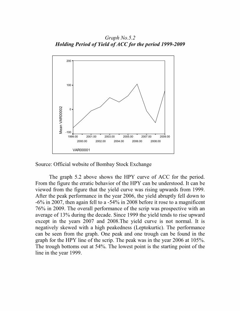
As per table 5.2 above, the largest holding period yield was 105% inthe year 2006. In the first 3 years of the decade the yield was negative. In thefirst year 1999 the yield was -75%. But year after year it was reducing. It canbe viewed from the figure that the yield curve was rising upwards from1999. After the peak performance in the year 2006, the yield abruptly felldown to -6% in 2007, then again fell to a -54% in 2008 before it rose to amagnificent 76% in 2009. The overall performance of the scrip wasprospective with an average of 13% during the decade. Since 1999 the yieldtends to rise upward except in the years 2007 and 2008.The yield curve isnot normal. It is negatively skewed with a high peakedness (Leptokurtic).For five years the scrip was earning negative holding period yield. The otherfive years it was making positive holding period yields. The performancecan be seen from the graph No.5.2 below. The lowest holding period yieldswere earned in 1999. Since 1999 the holding period yield was raising at rateof 200%. The year 1999 had a disastrous effect on the HPY of the company.On the contrary, year 2006 was highly prospective.

YEAR CL OP HPR HPY1999 248.25 1010 0.25 -752000 159 268 0.59 -412001 151.8 160.6 0.95 -52002 165.1 147.4 1.12 122003 245.55 164.25 1.49 492004 338.7 258.65 1.31 312005 534.2 341.5 1.56 562006 1085.55 530.5 2.05 1052007 1024.5 1092.4 0.94 -62008 477.9 1028.1 0.46 -542009 871.5 495.9 1.76 76

AM 13.45

Graph No.5.2Holding Period of Yield of ACC for the period 1999-2009


The graph 5.2 above shows the HPY curve of ACC for the period.From the figure the erratic behavior of the HPY can be understood. It can beviewed from the figure that the yield curve was rising upwards from 1999.After the peak performance in the year 2006, the yield abruptly fell down to-6% in 2007, then again fell to a -54% in 2008 before it rose to a magnificent76% in 2009. The overall performance of the scrip was prospective with anaverage of 13% during the decade. Since 1999 the yield tends to rise upwardexcept in the years 2007 and 2008.The yield curve is not normal. It isnegatively skewed with a high peakedness (Leptokurtic). The performancecan be seen from the graph. One peak and one trough can be found in thegraph for the HPY line of the scrip. The peak was in the year 2006 at 105%.The trough bottoms out at 54%. The lowest point is the starting point of theline in the year 1999.

VAR00001

2009.002008.00

2007.002006.00

2005.002004.00

2003.002002.00

2001.002000.00

1999.00

Mea

n VA

R00

002

200

100

0

-100

Table No.5.3Annual Return of ACC for the period 1999-2009

Year Annual Return1999 0.182000 -0.132001 0.032002 0.062003 0.212004 0.132005 0.192006 0.322007 0.012008 -0.252009 0.27

AM= 0.09


Table No.5.3 above, shows the rate of return earned by the scrip from1999 to 2009. On an average the scrip had earned a return of 0.09%. Exceptin 2000 and 2008 it had performed well. In 1999 the annual return of ACCwas 0.18%. In 2009 it rose to 0.27. The rate of growth in the annual rate was1.5 times. In two years ACC had negative annual returns. The annual returnwas registered in 2006 as 0.32% and the lowest 0.25% in 2008.Year 2008was worst for ACC. The graph also elucidates the highly fluctuating natureof the return. From Table No.2 and Table No.3 It can be found that the HPYwas stable and fluctuated moderately while the daily return made violentzigzags. In the case of annual return year 2008 played havoc. It was the mostdisastrous year in the decade for the company as far as annual returnsconcerned.

Graph No.5.3Annual Return of ACC for the period 1999-2009


The Graph 5.3 above, shows the behavior of the annual return ofACC. The curve was erratic, having lots of ups and downs and formation ofa peak and two troughs. From the graph it can be seen that the negativereturn in 2008 was the major fall in the decade for the stock ACC. Annualreturn line of ACC begun from higher point at Y-axis.Then it sharply fellbelow -1% in year 2000. Then it rose to 0.2% in 2004.After some minorzigzag again it rose to the maximum in 2007. Immediately then the annualreturns line fell sharply to the bottommost point in 2008. In 2009 annualreturns recovered from the depression and went up comfortably. In this waythere were full of ups downs in the movement of the annual return. In 2007the annual return was at the peak. But in the next year 2008 it sharply fell.Again in 2009 the return went up. Annual returns never stay permanent. Itwas moving violently rousing uncertainty and concern to the stake holdersand share holders. The annual returns of ACC were found highly volatileduring the period.

VAR00003

2009.002008.00

2007.002006.00

2005.002004.00

2003.002002.00

2001.002000.00

1999.00

Mea

n V

AR

0000

7

.4

.3

.2

.1

-.0

-.1

-.2

-.3

2. APOLLO TYRES

Table No.5.4Summary statistics of ACC from 1999 to 2009


Table No.5.4 above shows that the average return of the Apollo Tyreswas 0.10% which was slightly less than the market rate of return. Theestimated return represented by the HPY for the said period was 24.64. TheArithmetic Mean return of the company is considerably lower than thedecade’s holding period yield. The return is highly and negatively skewed ata rate of -4.089. During this period the company had made a maximumreturn of 25.94% and a smallest return of -89.4%. The range of the largestand smallest was 115.34. This shows that the scrip’s return was highlyfluctuating. The company had a high standard deviation of 3.81. Variancealso is high (14.54).The correlation between the company and the market islow as shown by the parameter r = 0.009. The value of kurtosis was 112.858.It signifies a greater amount of peakedness in the distribution. It is that ofLeptokurtic. The scrip’s relative volatility beta is 0.02. It is lower than themarket beta of 1.0. The beta coefficient is insignificant. R2 value of thecompany 0.0004 tells that 99.6% of the return is unexplained and only 0.004% is explained by the market. The scrip is not greatly influenced by themarket.

Average return 0.10% Skewness -4.089σ 3.81 Variance 14.54L 25.94 cov 0.06S -89.4 kurtosis 112.858Range 115.34 cor. 0.009Beta 0.02

R2 0.0004 HPY 24.64

Market return 0.11

Graph No.5.4Daily return of Apollo Tyres for 2642 days


The Graph 5.4 above shows the fact that the return from the companywas moderately distributed. The substantial portion of the daily return hadoccurred on and around X-axis or zero line. Occasional upheavals were alsofound off the abscissa. But they were only errors. The major chunk of returncould be located in between 0 and 5±. The lowest one day return was shownon the right hand side of the figure. Excessive hump can be seen on the lefthand side indicating negative skewness. As the standard deviation 0f thescrip 3.81 revealed there was high volatility in the daily returns. The graphshows the fact that the daily return has full of events with numerous violentvibrations about and around the mean returns. It shows that the daily returnwas not stable and regular. On the contrary, it was fluctuating and unstable.

Case Number

2,6422,503

2,3642,225

2,0861,947

1,8081,669

1,5301,391

1,2521,113

974835

696557

418279

1401

Val

ue V

AR

0000

2

40

20

0

-20

-40

-60

-80

-100

Table No.5.5Holding period yield of Apollo for the period 1999-2009

YEAR OP CL HPR HPY1999 64.85 159.05 2.45 1452000 171.75 88.55 0.52 -482001 89.2 79.9 0.9 -102002 76.8 134.2 1.75 752003 134.75 258.05 1.92 922004 275.15 235.75 0.86 -142005 239 278.4 1.16 162006 279.45 352.9 1.26 262007 348.35 53.8 0.15 -852008 57.9 19.85 0.34 -662009 20.35 48.8 2.4 140

AM 24.64


Table No.5.5 above shows, that the HPY of Apollo on an average was24.64%. In 1999 the HPY was 145%. In 2009 it was 140%. The HPY haddecreased by 3.44% during this 10 year period. The HPY was the highest in1999 with 145%. The lowest HPY was registered in 2007 as -85%. The year2007 was worst for the stock Apollo. In 5 years the scrip incurred negativeHPY and the other 5 years it had made positive HPY. Year 1999 was themost prosperous for Apollo. The HPY on an average was declining since1999. The years 2007 and 2008 had disastrous impact on the holding periodyields of the scrip. The performance 2009 was sudden recovery from thepreceding years’ great falls. Therefore the performance of the year 2009cannot be expected to be stable overtime. The history of the HPY for theentire period also did not support such a surmise. The Holding period Yieldof Apollo was full of uncertainties and volatilities during the period. Nothingcould be predicted.

Graph No.5.5Holding Period Yield Apollo for the period 1999-2009


Graph No.5.5 above, Shows that Apollo’s yield in the year 1999 was145%. In 2000 the HPY sharply fell and went down below the X-axis to theextent of -48%. But from 2001 onwards the HPY tended to go up. In thisway between 1999 and 2009 the HPY widely fluctuated in zigzag manner. In2009 again the holding period yield went up showing a prospective future.On an average in the meantime the company secured an overall HPY of24.64 during the decade. It is to be noted that the overall tendency ofApollo’s HPY is to decline since 1999. In the beginning and end of thedecade only the scrip could make outstanding HPY. They could beconsidered only chance performance. In between these two extreme cases inall other years the scrip’s HPY line was fluctuating and swinging up anddown in an indecisive way creating full of uncertainties. This can be viewedfrom the graph. Four peaks and four troughs could be seen in the movementof the HPY line indicating sporadic volatility in the holding period yield ofthe Apollo.

VAR00003

2009.002008.00

2007.002006.00

2005.002004.00

2003.002002.00

2001.002000.00

1999.00

Mea

n V

AR

0000

4

200

100

0

-100

Table No.5.6Annual return of Apollo for the period 1999-2009


Table No.5.6 above, shows the annual rate of return earned by thescrip Apollo from 1999 to 2009. On an average the scrip had earned a returnof 0.10%. Except in 2000, 2004, 2007 and 2008 it had performed well. In1999 the annual return of ACC was 0.50%. In 2009 it decreased to 0.43%.The rate of fall in the annual rate was 14 %. In 4 years Apollo had negativeannual returns. The largest annual return was registered in 1999 as 0.50%and the lowest -0.36% in 2008. Year 2008 was worst for Apollo. The annualreturn table of Apollo was very much similar to the HPY table. Years 2007and 2008 yield negative annual returns consecutively. Its impact on theannual returns of the entire period was very high. Even though in 2009 arecovery from previous years’ debacle was made, there was no sign that itwould be repeated in the future. From 1999 to 2009 the annual return of thestock was showing a tendency of declining year after year. Every year therewas only uncertainty about the return whether positive or negative.

Year Annual Return1999 0.502000 -0.182001 0.012002 0.292003 0.322004 -0.022005 0.082006 0.122007 -0.142008 -0.362009 0.43

AM 0.10

Graph No.5.6Annual return of Apollo Tyres for the period 1999-2009


The Graph 5.6 above shows the behavior of the annual return ofApollo. The curve was erratic, having lots of ups and downs and formationof a peak and two troughs. From the graph it can be seen that the negativereturn in 2008 was the major fall in the decade for the stock ACC. Theannual return line started well from a high point on Y-axis in 1999. Thenimmediately it falls below zero line in deep in 2000. Then it recovers andgoes up in the next years and reaches the maximum in 2003. Then abruptly itswings downwards below zero in 2004 itself. Then it recovers in 2005 andreaches another peak in 2006. There from it again make a somersault andfalls sharply below zero return point and reaches the bottommost showingthe minimum annual return for Apollo. In this way the annual return wasgoing up and down year after year recurring creating chaos and uncertaintyin the occurrence of annual returns for the company. It indicated themagnitude of volatility in the annual return of the stock.

VAR00003

2009.002008.00

2007.002006.00

2005.002004.00

2003.002002.00

2001.002000.00

1999.00

Mea

n V

AR

0000

5.6

.4

.2

-.0

-.2

-.4

-.6

3. ARVIND MILLS

Table No.5.7Summary statistics of Arvind Mills from 1999 to 2009


Table No.5.7 above shows that Arvind Mill’s average annual returnwas 0.07%. But expected return based on the past 10 years performance asshown by the holding period yield was 14.45%. On an average thecompany’s earnings were lower than the expected. During the same periodthe market return was recorded as 0.11% which was much more than thecompany’s return 0.07%. The standard deviation 3.86 and variance 14.9were significant and signals fluctuation in returns from the average. Duringthis period company earned a maximum of 37.5% return and went as low as-24.12% returns. The return ranged to a total of 61.26. It reveals the tightbond of the returns with the mean. The dispersion of the individual returnwas not wide and scattered from the mean return. The distribution of returnwas not normal. The positive skewness measured as 0.77 shows the fact thatthe distribution was positively skewed. The degree of skewness was veryhigh. The kurtosis worked out was 7.35. It shows the presence of apeakedness of leptokurtic. The correlation coefficient of the company’sreturn with the market was -0.33. It denotes the fact that the correlation isnegative with the market index and significant. The relative volatility of thescrip with the market as denoted by the beta was -0.71. It means thecompany behaved less than proportionately and inversely with the market.The risk of Arvind Mills is not more than the market portfolio. The R2 value

Average return 0.07% Skewness 0.77σ 3.86 Variance 14.9L 37.5 cov -2.28S -24.12 kurtosis 7.35Range 61.26 cor. -.33Beta -0.71 HPY 14.45R2 0.1089

Market return 0.11

0.109 tells the fact that only 11% of the variance 14.9 was explained by themarket and 89 % was unexplained by the market.

Graph No.5.7Daily return of Arvind Mills for 2642 days

Aravind mills

Daily Returns

Case Number

2,6232,485

2,3472,209

2,0711,933

1,7951,657

1,5191,381

1,2431,105

967829

691553

415277

1391

Value

VAR0

0001

50

40

30

20

10

0

-10

-20

-30


Graph.5.7 shows greater fluctuation in the daily return ofAravind Mills. It can be found that almost all values fall within therange of 0%-5% plus or minus. Largest value and smallest value canalso be noted on some exceptional days from the graph. The valueswere thronging about the average. The distribution is tightly knittedwith some occasional exceptional behavior. The substantial portion ofthe daily return had occurred on and around X-axis or zero line.Occasional upheavals were also found off the abscissa. But they wereonly errors. The major chunk of return could be located in between 0and 5±. The lowest one day return was shown on the right hand sideof the figure. Excessive grouping of returns can be seen on the righthand side indicating positive skewness. As the standard deviation 0fthe scrip 3.9 revealed there was high volatility in the daily returns.The graph shows the fact that the daily return has full of events withnumerous violent vibrations about and around the mean returns. Itshows that the daily return was not stable and regular. On thecontrary, it was fluctuating and unstable.

Table No.5.8Holding period yield of Arvind Mills for the period 1999-2009


Table No.5.8 above shows, that the HPY of Arvind Mills on anaverage was 14.45%. In 1999 the HPY was -37%. In 2009 it was118%. The HPY had increased by 4.2 times since 1999 during this 10year period. The HPY was the highest in 2002 with 141%. The lowestHPY was registered in 2008 as negative 85%. The year 2008 wasworst for the stock Arvind. In 6 years the scrip incurred negative HPYand the other 4 years positive HPY had been earned. Year 2002 wasthe most prosperous for Arvind. Year 2008 had played havoc to theHPY of the company. The HPY on an average was declining since1999. The years 2005, 2006 and 2008 had disastrous impact on theholding period yields of the scrip. The performance 2009 was suddenrecovery from the preceding years’ great falls. Therefore theperformance of the year 2009 cannot be expected to be stableovertime. The history of the HPY for the entire period also did notsupport such a surmise. Because of most of the years the holdingperiod of Apollo was negative. The Holding period Yield of Apollowas full of uncertainties and volatilities during the period. Nothingcould be predicted.

YEAR OP CL HPR HPY1999 39.7 25.05 0.63 -372000 24.25 13.4 0.55 -452001 13.3 9 0.68 -322002 9.1 21.95 2.41 1412003 21.95 22.55 1.03 32004 68.35 132.3 1.94 942005 134.5 95.6 0.71 -292006 96.8 51.7 0.53 -472007 52.3 90.55 1.73 732008 89.55 17.56 0.2 -802009 17.95 39.1 2.18 118

AM 14.45

Graph No.5.8Holding Period Yield of ArvindMills for the period1999-2009


The graph 5.8 above shows the HPY curve of Arvind for theperiod from 1999 to 2009.. From the figure the erratic behavior of the HPYcan be understood. It can be viewed from the figure that the yield curve wasrising upwards from 1999. From 1999 to 2009 Arvind’s stock faced 4 peaksand 4 troughs. The HPY curve was highly fluctuating. The overall tendencyof the HPY line was to decline. it could be seen that most of the years theHPY line of the company was going up and down along the x-axis. Despitethis the overall performance of the company was prospective by securing14.5%. The performance of the company in 2009 was impressive while theyear 2008 was worst.

In theend of the decade and occasionally in some years only the scripcould make outstanding HPY. For every rise immediate fall was experiencehy the scrip in the case of HPY. Whenever positive HPY was recorded itwas as if a chance performance. In all years the scrip’s HPY line wasfluctuating and swinging up and down in an indecisive way creating full ofuncertainties. This can be viewed from the graph. Four peaks and fourtroughs could be seen in the movement of the HPY line indicating sporadicvolatility in the holding period yield of the Apollo.

VAR00003

2009.002008.00

2007.002006.00

2005.002004.00

2003.002002.00

2001.002000.00

1999.00

Mea

n V

AR

0000

4

200

100

0

-100

Table No.5.9Annual return of Arvind Mills for the period 1999-2009

Year Annual Return1999 -0.112000 -0.182001 -0.032002 0.442003 0.492004 0.332005 -0.102006 -0.202007 0.272008 -0.522009 0.41

AM 0.07


Table 5.9 shows the average annual return of Arvind Mills. During the1999-2009 periods in the initial three years the company had made negativereturns. The average annual return was 0.07 per cent. In the year 2002 thecompany gained a return of 0.44%.In 2004 it made the maximum for thedecade 0.49%. In 1999 the annual return of Arvind Mills was -.11%. In 2009it made a return of 0.41%. Since 1999 the annual return of the scip wasincreasing by 4.7 times. In 1999 the annual return was negative. For sixyears the stock was making negative returns. Only four years it was makingpositive annual returns. It all amounts to the prevalence of high uncertaintyin the occurrence of the annual returns of Arvind Mills. There was chaos inthe distribution of annual returns for the stock for the period. Due to thischaos it becomes difficult to predict the future annual returns. Potentialinvestors would be panic as to whether to invest on the stock or not. Such anamount of uncertainty in annual returns of the company was prevailing over.

Graph No.5.9Annual return of Aravind Mills for the period 1999-2009


It could be seen from the graph No.5.9 that the average annual returnof the company Arvind Mills from 1999 onwards rose from negative returnsto positive and reached the maximum in 2003. Then the annual return linewas falling with lot of minor ups and down. The line had been finally fallento the lowest and worst in 2008. Then again the line recovered and went upin 2009. The annual return line of Arvind stock was highly volatile duringthe period.

The scrip’s annual return curve was starting from low minus point onY-axis. Then it rose to a peak with much hesitation in 2003. There from itfell sharply and abruptly crossing zero line down to a trough in 2006. Thenthe annual return line again rose to a higher point in 2007. Then fell down toanother major trough which was minimum annual returns for the firm in thedecade in 20008. Annual return line in this way had a travail of going up anddown with full of twists and turns of short-living in nature throughout itslength. It all indicates high level of uncertainty prevailing in the occurrenceof annual returns of the company.

VAR00003

2009.002008.00

2007.002006.00

2005.002004.00

2003.002002.00

2001.002000.00

1999.00

Mea

n VA

R00

005

.6

.4

.2

-.0

-.2

-.4

-.6

4. Ashok Leyland

Table No.5.10Summary statistics of Ashok Leyland from 1999 to 2009


Table 5.10 shows, that the average return earned by Ashok Leylandduring the period was 0.11% which was identical to the market return. TheHPY was 48.27%. The HPY is much higher than the market return of0.11%. As the HPY is a proxy for estimated return the company’s averagereturn was disappointing. During the decade of 1999-2009 the companyearned a largest return of 18.22. The smallest for the same period was -89.2.The return for the period was wavering between these two values giving wayto high level of uncertainty and fluctuations. The range 107.94 is bignumber representing high volatility of the returns. The distribution of thereturn was not normal. It is negatively skewed to the extent of -4.53. Notonly negatively skewed but also had a leptokurtic peakedness. The beta ofthe company reveals the systematic risk of the company. The beta -0.011 isnegative, which only rarely happens, and lower than the market proxy ofB.S.E30. The R2 value given confirms it. The R2 value 0.005 is insignificantin the sense that the only 0.005% of the total variance was explained by themarket, the remaining 99.5% was unexplained by the market. It means thestock’s market-related risk is insignificant.

Average return 0.11% Skewness -4.53σ 3.9 Variance 22.07L 18.22 cov -0.034S -89.2 kurtosis 115.24Range 107.94 cor. -0.005Beta -0.011R2 0.005 HPY 48.27%

Market return 0.11%

Graph No.5.10Daily return of Ashok Leyland for 2642days


It can be seen from the graph 5.10 above, that most of the valuesrange between 0-5 plus or minus. The maximum return is 18.22% andminimum -89.2% could be observed from the graph. Minor fluctuationaround the x-axis could be traced out. The return was highly fluctuating asshown by the standard deviation and variance. The daily returns were thicklycoated on either sides of the zero-line. It means the actual returns werearound the mean returns. Still enormous minor and major vibrations werefound about the zero line indicating high level of fluctuations in thedistribution of daily return. The standard deviation of Ashok Leyland was3.79. It is well above 3. Standard deviation above 3 is significant. Theimplication of it was that there were intense and violent errors about themean daily returns signaling high degree of price and return volatility. Onthe left side of the distribution undue swarming or humping could be seen inthe picture indicating negative skewness. It was due to the fact that thedistribution was not symmetrical.

ASHOK LEY

DAILY RETURN

Case Number

2,6422,503

2,3642,225

2,0861,947

1,8081,669

1,5301,391

1,2521,113

974835

696557

418279

1401

Valu

e VA

R00

003

40

20

0

-20

-40

-60

-80

-100

TableNo.5.11Holding period yield of Ashok Leyland for the period1999-2009

YEAR OP CL HPR HPY1999 44.8 114.05 2.55 1552000 123.15 43.75 0.36 -642001 44.6 69.65 1.56 562002 68.7 99.15 1.44 442003 98.2 293.7 2.99 1992004 294 24.4 0.08 -922005 24.65 31.85 1.29 292006 31.8 45.45 1.43 432007 46.25 52 1.12 122008 52.15 15.02 0.29 -712009 15.5 49.55 3.2 220

AM 48.27


Table 5.11 shows that the company was making a holding periodyield of 48.27% for the period 1999-2009. Except 3 years the companymakes good estimated returns during the decade. The maximum HPY 220%was obtained in the year 2009. In the years 2003 and 1999 HPY earned was199 and 155% respectively. In 2009 the company’s performance wasexceptionally good. In 1999 the HPY of Ashok Leyland was 155%. In 2009it was 220%. There was an overall growth of 42% in the HPY since 1999. Inthree years the HPY was negative. For seven years the HPY was positive.The lowest yield -71% was made in the year 2008. The highest HPY wasoccurred in 2009. The year 2008 was disastrous for the HPY of the stock. Atthe same time the year 2009 was prospective for the firm.On average thetrend of the HPY was rise upwards.

Graph No.5.11Holding period yield of Ashok Leyland for the period 1999-2009


It can be seen from the graph 5.11 that in 1999 the company wassliding from 155% to reach below cutting the x-axis. Then after 2000 it wentup to 199% in 2003. There from it fell sharply down to the all time low in2004. After that it recovered and gathered momentum better its position bygaining the all time best of 220% in 2009. As the graph shows the HPY ofAshok Leyland had full of twists and turns during the period. The yieldnever stayed anywhere more. It was always instable. There was one peak in2003. Immediately after that a deep trough was followed in 2004. Then in2005 the HPY went up and in 2007 tended to fall down and in 2008 the HPYfell to the all time low. In this way the HPY of Ashok Leyland goes up anddown all time without settling for some time anywhere. It all shows thevolatility of the HPY of the stock. The line HPY starts from a high point. Itends also in a high point. Between these points it had endless ups anddowns. This was due to chaos and uncertainty in the distribution of theholding period yield of the company.

VAR00003

2009.002008.00

2007.002006.00

2005.002004.00

2003.002002.00

2001.002000.00

1999.00

Mea

n V

AR

0000

4

300

200

100

0

-100

-200

Table No.5.12Annual return of Ashok Leyland for the period 1999-2009

Year Return1999 0.502000 -0.332001 0.262002 0.192003 0.472004 -0.402005 0.132006 0.192007 0.082008 -0.432009 0.54

AM 0.11


As per table 5.12, from 1999 to 2009 the company was making anannual rate of 0.11%. Seven years it made positive returns and 3 yearsnegative. In 1999 the annual return was 0.50%. In 2009 it was 0.54%. Theannual return was growing by 8% since 1999. The highest positive returnwas in 2009 that is 0.54% and the lowest return it earned was in 2008 that is-0.43%. The Year 2008 was worst for Ashok Leyland. The year 2008 haddone much harm to the annual returns to the company. In the decade thestock was making steadily positive returns. Only in 3 years it succumbed tonegative results. High volatility was there in the flow of annual return to thestock. High and lows were coming in alternating years. Ups and downs werecoming year after year. There was uncertainty in the occurring of annualreturns. It was not possible to predict the behavior of annual returns due tothe high volatility.

Graph No.5.12Annual return of Ashok Leyland for the period 1999-2009


The graph 5.12 shows that the return of the stock Ashok Leyland wasin a zigzag manner as in a see-saw. The return went up and down of the zeroline in alternating years. It reveals greater risk. Sudden uprising and declinecan be observed. The highest positive return of the company was earned inthe year 2009 and lowest was in 2004. Between 1999 and 2009 a sporadicvolatility was found with the pattern of return. As the graph had shown therewere three peaks and three troughs occurred in alternating years. It becamecyclical. This volatility in annual returns can be found repeating year afteryear. It shows the high volatility prevailing in the distribution of annualreturns in the decade. It was starting from a high point in 1999. Then, theannual return was suddenly swinging down to below zero line in 2000. Thenagain recovered and went up to a small peak in 2001. In 2002 it further wentup to a major peak in 2003. In 2004 it abruptly had fallen to deep trough. Inthis way the annual returns were never stable throughout the decade

VAR00003

2009.002008.00

2007.002006.00

2005.002004.00

2003.002002.00

2001.002000.00

1999.00

Mea

n V

AR

0000

5

.6

.4

.2

-.0

-.2

-.4

-.6

5. ASIAN PAINTS

Table No.5.13Summary statistics of Asian Paints from 1999 to 2009


As per table 5.13 above, the average return of the stock AsianPaints for 10 years was 0.09% which was less than the average return of themarket 0.11% for the same period. The HPY was 23.27%. The company wasunder performing. The company’s performance was much below of whatwas expected of it. The large and small value reveals that the return was notwidely scattered. The dispersion from the mean is normal. The standarddeviation 2.09 is not significant. Therefore the company is making a stablereturn for the period. The return varies in between positive 11.61% and anegative 36.19% amounting to range of 47.8. Hence the distribution wastighter. The skewness -2.9 is significant . It says that the return is not onlyasymmetrical but negatively skewed. The kurtosis 57.87 signals leptokurticform of peakedness. The correlation 0.006 between the company and themarket is insignificant. The systematic risk denoted by beta 0.007 is low. R2

says that 1% of the variance is explained by the market. 99% variance isunexplained by the market. The scrip was not much market-related duringthe period.

Average return 0.09% Skewness -2.9σ 2.09 Variance 4.35L 11.61% cov 0.02S -36.19% kurtosis 57.87Range 47.8 cor. 0.006Beta 0.007R2 0.000036 HPY 23.27

Market return 0.11

Graph No.5.13Daily return of Asian Paints for 2642 days


It can be seen from the above figure that the return is negativelyskewed. The largest return 11.61 and the smallest 36.19% could be locatedfrom the graph. The tightness of the distribution could also be discerned. Lotof minor fluctuations around the zero line can be viewed. The volatility ofstock return about the mean value can be observed. The values were foundlying within a range of 0-5%±. The values were thickly coated along the lineof X. Some values had shown tendency to fall down to the line of abscissaoccasionally can also been located from the figure. Undue humping ofvalues on the left hand side of graph can be seen due to the presence ofnegative skewness of daily returns. From the graph it could be understoodthat the distribution of the daily returns was not symmetrical. Minorvibrations could be located on either side of the mean returns. The lowestand highest daily returns were found in the graph. The volatility in the dailyreturns was not very strong. But small errors were running around the meanof daily returns.

Case Number

2,6422,503

2,3642,225

2,0861,947

1,8081,669

1,5301,391

1,2521,113

974835

696557

418279

1401

Valu

e VA

R00

002

20

10

0

-10

-20

-30

-40

Table No.5.14Holding period yield of Asian paints for the period1999-2009

YEAR OP CL HPR HPY1999 285.5 370 1.3 302000 389.95 276.6 0.71 -292001 272 271.5 1 02002 265.85 324.65 1.22 222003 324.5 336.15 1.04 42004 336.7 320.15 0.95 -52005 320 577.4 1.8 802006 589.75 733.55 1.24 242007 740.85 1102.55 1.49 492008 1136.3 895.1 0.79 -212009 888 1796.25 2.02 102

AM 23.27


As per table 5.14above, the average holding period yield of AsianPaints was 23.27% which was the expected return of the company. The HPYwas the highest in 2009 with 102%. The lowest was in the year 2000 with -29%. In 2001 the company made no yield at all. In 1999 the HPY of AsianPaints was 30%. In 2009 it was 102%. The HPY had increased 3.4 timessince 1999. In 3 years the HPY was negative. In 7 years the HPY waspositive. The tendency of the HPY was to grow. Even though the companyhad made positive HPY in almost all years in the decade the magnitude ofthis was highly uncertain. Despite the fact that Asian paints made good HPYin the entire period, the HPY was highly erratic. There was no certainty inthe occurrence of the HPY. The pattern and magnitude of the HPY werehighly chaotic. The pattern was uncertain because in a year the HPY was80%, in another year it was 5%. In still another year the HPY was zero. Insome years the HPY was positive and in some other year it was negative. Inthis way the pattern and the magnitude of the HPY of Asian paints had nocertainty. This chaotic behavior entails high level of volatility to the scrip ofAsian paints.

Graph No.5.14Holding Period Yield of Asian Paints for the period 1999-2009


It could be seen from the graph 5.14 that the HPY of Asian Paintswas highly volatile throughout the decade. As in a see-saw the HPY wasswinging went up and down with constancy throughout the period. But theoverall tendency could be located from the figure that the HPY continuouslygrowing upward. In the year 2009 HPY had been reached a new height in itsperformance. The graph vindicates what was said earlier about the HPY ofAsian Paints. The HPY was driving towards persistently higher and higherpoints of yields. But here and there it confronted resistance and broke down.But the HPY was relentlessly was going towards better results. This thrust ofthe holding period yields of Asian Paints could be learnt from the figure. Inthe travel it faced four minor major troughs and similar peaks also. Thenumber of peaks and troughs tell the intensity of the volatility in thedistribution of the HPY. More ups and downs were found in the case ofAsian paints in varying pattern and magnitude. The more it is, the high thevolatility of the HPY.

VAR00003

2009.002008.00

2007.002006.00

2005.002004.00

2003.002002.00

2001.002000.00

1999.00

Mea

n V

AR

0000

4

120

100

80

60

40

20

0

-20

-40

Table No.5.15Annual return of Asian paints for the period 1999-2009


As per table 5.15 above, the average annual return of the stock AsianPaints for the period 1999-2009 was 0.09%. In 1999 the annual return was0.15%. In 2009 it was 0.32%. The annual return during the period had beenincreased at the rate of 113% since 1999. In 3 years the annual return wasnegative. In 7 years it was positive. The annual return was the highest in2009 and lowest in 2000. The overall tendency of the annual return was togrow. As shown by the table, the annual returns’ behavior was similar to theholding period yields of Asian paints. While the annual return in 1999 waspositive, it went negative in the next year itself in 2000. Then in the nextyear there was no annual return at all in 2001. Then in 2002 and 2003 thescrip made nominal annual return. After that again 2004, the returns becamenegative. After that there was steady progress in the annual returns till 2008.In 2008 again it earned negative returns. In this way negative positivereturns were earned by the stock in an alternating way. This was due to thehigh price volatility in the market. Therefore high level of uncertainty andchaos found with the annual return of Asian Paints.

Year Annual Return1999 0.152000 -0.082001 0.002002 0.092003 0.052004 -0.012005 0.252006 0.112007 0.192008 -0.072009 0.32

AM 0.09

Graph No.5.15Annual Return of Asian Paints for the period 1999-2009


As Graph 5.15 showed, in 1999 annual return of Asian paints wasvery high. There after it declined. From 1999 to 2009 the annual return linewas moving across wide fluctuations. Therefore the line of annual returnwas erratic and zigzag. Though the trend was to grow up, the annual returnwas highly volatile in nature. While the annual return in 1999 was positive,in 2000 it went negative. It could be easily found that the fluctuations inannual returns from the graph above. From the beginning of the annualreturn curve to its end in 2009, it went across numerous ups and downs oneafter another. There was no stability to any trend. There was no trend at all.In one year the annual return was positive. In the next year itself it turns tothe opposite. Still the persistent trend that was underlying could be locatedfrom the graph vividly. It was that of going up. But there prevailsuncertainty and chaos as to the accuracy about the occurrence of the returnswhether it would be negative or positive or whether it would be a bigamount or low amount. This form of uncertainty was there in the pattern andmagnitude of the annual returns of Asian Paints.

VAR00003

2009.002008.00

2007.002006.00

2005.002004.00

2003.002002.00

2001.002000.00

1999.00

Mea

n V

AR

0000

5

.4

.3

.2

.1

0.0

-.1

-.2

6. BALLARPUR INDUSTRIES

Table No.5.16Summary statistics of Ballarpur Industries from 1999 to 2009


As per table 5.16 the average return of Ballarpur was 0.08% whichwas lower than the market average of 0.11%. The expected return based onthe HPY was 16.64%. Company’s average performance for the ten yearperiod was lower than the HPY. The dispersion from the expected value wassignificant as expressed by the standard deviation 3.6. The scrip had made amaximum return of 21.69% and minimum of -79.61% during this period.This amounts to total range of 101.3 which shows a greater amount ofvariance. The values greatly vary in between the large and small. There isgreater amount of uncertainty in the occurrence of return. The skewness -3.49 was significant in the sense that the distribution was negatively skewed.The variance also tells the same tales that there is greater fluctuation in thereturn stream of the company. The variance 13 was significant. The kurtosis90.41 signals peakedness to the character of leptokurtic. The correlation co-efficient 0.023 is not important. The beta 0.0464 does not express anyserious systematic risk. R2 value 0.0005 is insignificant that the variancemainly owing to the own performance of the company.

Average return 0.08% Skewness -3.49σ 3.6 Variance 13L 21.69 cov 0.148S -79.61 kurtosis 90.41Range 101.3 cor. 0.023Beta 0.0464R2 0.0005 HPY 16.64

Market return 0.11%

Graph No.516Daily return of Ballarpur for 2642 days


Graph 5.16 shows the pattern of the daily return for the company forthe ten year period from 1999 to 2009. The daily return was thickly packedalong the X-axis with few exceptions. Barring some occasional outspreadsthe return in general was permeated along the zero line. The return wasspread within a range of 0-5%. The high and low values can be located fromthe graph easily. The daily returns had lot of minor variations around andabout the line of X axis. Excessive grouping of values can be located on theleft hand side from the center of the zero line due to negative skewness. Thestandard deviation and variance of the daily returns were found significant.The varying trend of the individual returns from the mean could beidentified from the graph. The daily return was shown in the graph as thicklypacked. The density of the values could be grasped from the figure. Thedaily returns of Ballarpur industries were due to excessive price fluctuationsin the market for its stock.

BALLARPUR

DAILY RETURN

Case Number

2,6422,503

2,3642,225

2,0861,947

1,8081,669

1,5301,391

1,2521,113

974835

696557

418279

1401

Valu

e VA

R00

002

40

20

0

-20

-40

-60

-80

-100

Table No.5.17Holding period yield of Ballarpur for the period 1999-2009

YEAR OP CL HPR HPY1999 27.85 58.25 2.09 1092000 62.9 63.05 1 02001 64.4 40.9 0.64 -362002 40.2 43 1.07 72003 43 82.3 1.91 912004 83.2 93.95 1.13 132005 98.15 112.15 1.14 142006 112.95 107.5 0.95 -52007 109.35 173.4 1.59 592008 181.6 20.7 0.11 -892009 20 23.95 1.2 20

AM 16.64


The Table 5.17 shows the HPY of Ballarpur Industries for the periodfrom 1999 to 2009. The HPY of the stock on an average for the period was16.64%. In 1999 the HPY was 109%. In 2009 it was 20%. The HPY duringthe period had been declined by 82%. In 2000 the HPY was zero. The HPYwas largest in 1999 and smallest in 2008. The year 2008 was very bad forBallarpur Industries. In 3 three years Ballarpur earned negative HPY. In 7Years there was positive HPY. Generally, the tendency of the HPY was todecline. The HPY in the beginning and at the close of the decade showedgreater difference. The HPY from 109% in 1999 had fallen to a mere 20 %in 2009 after 10 years meant greater failure in the performance of the stockin the market. It might be due to the price volatility in the market. The stockearned positive yields in all seven years. Only in three years it was subject tonegative returns. But the impact of three years’ negative performance washighly detrimental. The year 2008 had done much damage to the HPY ofBallarpur.

Graph No.5.17Holding period Yield of Ballarpur for the period 1999-2009


The graph 5.17 shows that HPY line starts from a peak 109% in 1999 felldown to zero in 2000. It fell further below X-axis to -36 where it bottomedout for a recovery to another peak with 91% in 2003. Again it moveddownward and rose and fell sharply the all time low of -89% before it risesto 20% in 2009. Though HPY was positive in almost all cases except in 3years the overall tendency was to fall down. The HPY was erratic andmostly uncertain. The ups and down showed by the HPY denotes theexistence of high degree of volatility in returns during the period. Theadversity for the scrip Ballarpur Industries with lowest HPY in 2008 can beseen from the figure. The behavior of the HPY of Ballarpur Industries couldbe easily understood from a glance of the graph. It was highly volatile. Thecurve with numerous major and minor swings-downward and upward-hadsettled at relatively a lower point by showing the persistent trend as that ofdeclining over years.

VAR00007

2009.00

2008.00

2007.00

2006.00

2005.00

2004.00

2003.00

2002.00

2001.00

2000.00

1999.00

Mea

n VA

R00

008

200

100

0

-100

Table No.5.18Annual return of Ballarpur for the period 1999-2009

Year Annual Return1999 0.422000 0.112001 -0.132002 0.062003 0.282004 0.092005 0.092006 0.032007 0.222008 -0.532009 0.14

AM 0.07


The Table 5.18 shows the annual returns of Ballarpur Industries forthe period from 1999 to 2009. The annual returns of the stock on an averagefor the period were 0.07%. In 1999 the annual returns were 0.42%. In 2009it was 0.14%. The annual returns during the period had been declined by67%. The annual return was largest in 1999 and smallest in 2008. The year2008 was very bad for Ballarpur Industries. In 2 years Ballarpur earnednegative returns. In 8 Years there were positive annual returns. Generally,the tendency of the annual returns was to decline. In spite of the stock beingearned positive returns for seven years, the underlying trend was identifiedas that of declining. This was because of the frequent interruption by thedownswing in the annual returns. The downswing was due to nothing but theprice volatility in the market. The continuous earning of the annual returnswas now and then deterred by adverse changes in the stock price in themarket. That was why after making seven years positive returns the stockbecame unable to prosper.

Graph No.5.18Annual returns of Ballarpur for the period 1999-2009


The graph 5.18 shows, that the behavior of the annual average returnwas very similar to that of the HPY for the period. From 1999 to 2008 theaverage return tends to fall and reaches the all time low of the decade in2008. In 2009 a recovery was achieved and the annual average returnincreased to 0.14%. The curve of annual returns was highly volatile anderratic. The general trend of the annual return of Ballarpur was to decline.The curvature of the annual returns in the graph was shown as highly erratic.It was frequently disrupted and fractured by the downtrend. Frequentinterruptions marred the continuity of the annual returns line could be foundbroken. It was due to the wild uncertainties and fluctuations in the stockprices in the market. The price volatility in the market paved the way for theannual returns volatility since the returns were perceived from the prices ofthe stocks in the market. Therefore lower the price lower will be the returnsalso. As such the volatility was intense in the behavior of the annual returnsof Ballarpur Industries. This could be discerned from the nature of thecurvature of the annual returns curve in the graph. The curve had all thetravails of frequent disruptions and interruptions that was why the annualreturns could not be able to finish impressively in spite of seven yearspositive returns.

VAR00007

2009.002008.00

2007.002006.00

2005.002004.00

2003.002002.00

2001.002000.00

1999.00

Mea

n VA

R00

009

.6

.4

.2

-.0

-.2

-.4

-.6

7. CASTROL

Table No. 5.19Summary statistics of Castrol from 1999 to 2009


As per table 5.19 above the average return of Castrol was 0.02%which was lower than the market rate of return of 0.11%. Expected returnbased on the performance of the company in the decade was 4.82% whichwas much above the actual. The standard deviation 2.34 was not important.The actual would be almost near the average return. The range of variationbetween the largest and smallest value to the extent of 66.06 wasinsignificant. The variance 5.45 was below the point of significance. Thestandard deviation and the variance did not tell any significant volatility. Thedistribution of return as stated by the skewness -2.49 revealed the presenceof high asymmetry. The distribution was skewed negatively. The kurtosis71.1 is big and significant peakedness of the form of leptokurtic could beobserved. The beta value 0.008 was not significant. The relative volatilitybetween the company and the market was less. R2 value confirmed that lessthan 1% of the variance 5.45 was explained by the market and 99.99% wasunexplained.

Average return 0.02% Skewness -2.49σ 2.34 Variance 5.45L 17.67 Cov 0.025S -48.39 kurtosis 71.1Range 66.06 cor. 0.006Beta 0.008R2 0.000036 HPY 4.82

Market return 0.11%

Graph No. 5.19Daily return of Castrol for2642 days


The graph 5.19 showed that the daily return of Castrol Ltd coincided mostlywith the zero line and ranged between zero and plus or minus 5% asdepicted by the Graph. Extreme values occurred only occasionally. Thelowest return of -48.39% could be traced from the figure. The highest returnearned during the decade could also be located from the figure. It could beidentified that the return was highly negatively skewed. Lot of minorvolatility around and about the zero line can be seen. The daily returns ofCastrol were highly volatile during the period. The daily returns of the stockwas found in the graph as thickly pasted on either side of the mean returnThe mean return of Castrol was given in the summary statistics tableNo.5.19 as 0.02%. So it could easily be found that the earnings were denselypacked within the immediate range of 0-1%. Some values could also belocated outside this range up to 5%. But majority of values were shown inthe graph lying in between 0-1% range. The standard deviation of the returnswas not significant. The standard Deviation given in the summary StatisticsTable No 5.19 was 2.34. It only confirms the tightness of the distribution.Only minor insignificant fluctuations in earning could be seen from thegraph.

CASTROL

DAILY RETURNS

Case Number

2,6422,503

2,3642,225

2,0861,947

1,8081,669

1,5301,391

1,2521,113

974835

696557

418279

1401

Val

ue V

AR

0000

3

40

20

0

-20

-40

-60

Table No.5.20Holding period yield of Castrol for the period 1999-2009

YEAR OP CL HPR HPY1999 758.25 305.15 0.4 -602000 329.55 273.25 0.83 -172001 276.35 187.6 0.68 -322002 187.8 210 1.12 122003 209.65 237.9 1.13 132004 239.25 217.8 0.91 -92005 217.85 252.3 1.16 162006 254 227.9 0.9 -102007 223 360.65 1.62 622008 350.75 335.5 0.96 -42009 333.7 605.8 1.82 82

AM 4.82


Table 5.20 showed that The HPY of Castrol on an average for theperiod from 1999 to 2009 was 4.82%. In 1999 the HPY was -60%. In 2009 itwas 82%. The HPY had increase by 136% since 1999. In the initial threeyears of the decade the company made negative holding period yields. In theyear 1999 the return was the lowest to the extent of -60%. Then in 2000 itimproved a little but continued to earn negative HPY of -17%. The highestpositive return was earned in the year 2009 to the tune of 82%. On anaverage holding period yield for the 10 year period from 1999 to 2009 was4.82%. The holding period yield for 2009 was a high 82%. Still the overallholding period yield of the stock for the 10 year period was only 4.82%. Itwas due to frequent downside movement of the price of the stock in themarket. The growth in holding period yields was at times blocked by theoccurrence of negative returns. The traces of the volatility could be foundwith the holding period yields of the stock for the period.

Graph No.5.20Holding Period Yield of Castrol for the period 1999-2009


The graph 5.20 shows the pattern of the holding period yield Castrol.Since 1999 the yield was rising upwards. The trend of the HPY line is to goup in a stair step manner. From -60% in 1999 the HPY ascended to 82% in2009 gradually and successively year after year. The lowest HPY could belocated in the graph in the year 1999 and the highest in the year 2009. Thecurvature of the holding period yield curve shows that it was confronting alot of strife before it reached the end point. Frequent disruptions,downswings, resistance and all that pull the curve down from going up. Stillthe stock managed to finish positively at the end of the decade in a stair stepmanner. The simile stair-step was meaningful in every respect in the sensethat as in a stair-step for every step upward there will be immediate downstep. But generally the purpose of the stair-step is to go up. In the same waythe overall tendency of the holding period curve was to go up but frequentlyfacing down steps at every up step.

VAR00003

2009.00

2008.00

2007.00

2006.00

2005.00

2004.00

2003.00

2002.00

2001.00

2000.00

1999.00

Mea

n VA

R00

004

100

80

60

40

20

0

-20

-40

-60

-80

Table No.5.21Annual return of Castrol for the period1999-2009

Year Annual Return1999 -0.242000 -0.042001 -0.122002 0.052003 0.072004 -0.022005 0.082006 -0.032007 0.212008 0.022009 0.26

AM 0.02


Table 5.21 shows that annual return of Castrol in 1999 was -0.24%and in 2009 it was 0.26%. The lowest annual return was recorded in the year2004 as -0.02%. The annual return was highest in 2009 with 0.26%. From1999 onwards the negative return was improving and by 2002 it becamepositive to the tune of 0.05%. The last three years of the decade alsorecorded positive returns. The highest annual return was recorded in 2009.Castrol had made negative returns and positive returns in 5 years each. Theoverall result was that the company made a 0.02% return for the 10 yearperiod. The annual return also behaves in the same way as the HPY. It wasincreasing from -0.24% to 0.26%. The growth in the annual return wastremendous during the period in spite of frequent interruptions by theoccurrence of negative returns. The volatility that caused the negative returncreated lot of chaos and uncertainty in the occurrence of annual returns. Thetable gives details of high levels of volatility.

Graph No.5.21Annual return of Castrol for the period 1999-2009


From the graph 5.21 the behavior of annual return of Castrol could beunderstood. The annual return moves upward from the deep fall of negative0.24% to the topmost place of 0.26% in 2009 step by step year after year.The shape of the annual return line is like stair-step. The overall trend of theannual return for the decade is that of a steady growth from -0.24 to 26%.There were lots of ups and down throughout the period which were indicatedby the line of annual return. The behavior showed by the table could beunderstood from the graph. The graph represents high level of fluctuations inthe annual returns of the stock. The overall effect of the annual returns wasto go up. But at times the rise of the annual returns curve was checked anddisrupted by the downtrend movements. This caused the volatility in theannual returns. The consequence of it was that no one could predict theoccurrence of annual returns on the stock. The volatility was there in annualreturns of the company in respect of the timing and magnitude of it.

VAR00003

2009.002008.00

2007.002006.00

2005.002004.00

2003.002002.00

2001.002000.00

1999.00

Mea

n VA

R00

005

.3

.2

.1

-.0

-.1

-.2

-.3

8. CENTURY TEXTILES

Table No.5.22Summary Statistics of Century from 1999 to 2009


The summary statistics of Century Textiles for the period was shownby Table 5.22. On an average the company earns a return of 0.17% contraryto the expected 53%. The performance was better than the market return0.11%.The standard deviation 3.29 was significant. The largest rate of returnearned was 22.84% and the smallest rate was -24%. The breadth between thelarge and small was 46.84. The daily return varied in between this boundary.Therefore the return was tightly and closely bonded within the expectedvalue or mean value that is 0.17%. The chances for the wide variability arerare and remote. Therefore the standard deviation 3.98 does not tell muchvolatility. The distribution of return is positively skewed to the right. Themeasure of skewness 0.18 is not significant. The variance 15.82 issignificant. The kurtosis 2.8 denotes some amount of peakedness near toleptokurtic. The distribution is not symmetric. The co-efficient of correlation0.003 is not significant. The relative volatility of the company in relation tothe BSE represented by the statistic beta 0.01 was not significant. But therisk of the company vis-à-vis the market is lower. R2 only confirmed it.Accordingly 0.000009% of the variance was explained by the market.99.99% was explained by company’s own factors. The HPY which wasconstrued as the expected return over a period of 10 years is 53%. Howeverthe company’s average return was lower than HPY.

Average return 0.17% Skewness 0.18Σ 3.98 Variance 15.8L 22.84 cov 0.021S -24 kurtosis 2.82Range 46.84 cor. 0.003Beta 0.01R2 0.000009 HPY 53%

Market return 0.11%

Graph No.5.22Daily return of Century for 2642 days


In the Graph.5.22 over a period of 10 years on 2642 observation thedetails of the daily return of Century Textiles are shown. The daily returnwas found thickly packed along the X-axis. Barring occasional rise and fallhither and thither most of the daily return had occurred with range 0-8%±.The largest daily return could be noted at the 557th observation clearly.Similarly the smallest daily return was registered at the same level. Theskewness could also be located slightly to the right side. The daily returnshad high degree of volatility. A thick band of returns was densely formed oneither side of the mean value. The number of values surrounding the meanreturn was immense. The standard deviations variance of returns could beobserved from the graph. They are all significant. The daily returns were allhighly volatile in nature. The volatility could be seen from the graph.

CENTURY

DAILY RETURNS

Case Number

2,6422,503

2,3642,225

2,0861,947

1,8081,669

1,5301,391

1,2521,113

974835

696557

418279

1401

Val

ue V

AR

0000

4

30

20

10

0

-10

-20

-30

Table No.5.23Holding period yield of Century for the period1999-2009

YEAR OP CL HPR HPY1999 42.6 58 1.36 362000 62.6 42 0.67 -332001 43.95 37.65 0.86 -142002 38.2 49.4 1.29 292003 53.9 140.25 2.6 1602004 144.55 176 1.22 222005 186.45 299.65 1.61 612006 301.35 739.8 2.45 1452007 739.8 1170.45 1.58 582008 1207.6 166.65 0.14 -862009 175.1 528.05 3.02 202

AM 52.73


Table 5.22 above shows the holding period yield of Century Textiles forthe period 1999-2009. The largest HPY for the study period was 202% in theyear 2009. Lowest HPY was registered as -86% in 2008. Century Tex hadmade negative HPY in 3 years and positive returns in 7 years. The overalltendency of the HPY had been to rise upwards. In 1999 the HPY of Centurywas 36%. In 2009 it was 202%. The HPY had increased during this period ata rate of 461%. The tendency of the HPY was to grow. The average of HPYfor the decade was 53%. The year 2008 had detrimental impact on the HPYof the stock. The table showed the presence of high level of volatilitythroughout the decade.

Graph No.5.23Holding Period Yield of Century Textiles for the period 1999-2009


The graph 5.22 above shows the picturization of the facts analysedabove as to the HPY of Century Textiles. The high and low of HPY can beviewed from the graph clearly. There were 3 peaks and 3 troughs in thepicture. It reveals the thick and thin through which the company crossedduring the period. The high and low HPY happens with an alternatingregularity. The overall trend of the HPY was that of ever increasing. Theincreasing trend of the HPY was at times marred by the upswing anddownswing trends. It was due to major volatility in the market andconsequent volatility in the HPY. The second trough was depicted in thegraph was a major one. The year 2008 inflicted major impact on the HPY ofthe stock.

VAR00001

2009.002008.00

2007.002006.00

2005.002004.00

2003.002002.00

2001.002000.00

1999.00

Mea

n VA

R00

002

300

200

100

0

-100

-200

Table No.5.24Annual return of Century Textiles for the period 1999-2009


The table 5.23 shows the behavior of average annual rate return ofCentury Textiles during 1999-2009. In 1999 the company had annual returnof 0.27% whereas in 2009 it was 0.53%. The return of 2009 was the highestduring the study period. Lowest annual return was fetched in the year 2000to the tune of -0.06%. The highest positive annual return was 0.53% in 2009and the lowest return was in 2001with an amount of 0.06%. Only in twoyears the company had made negative returns. It made positive annualreturns in 8 years. So the trend was that the scrip regularly makes a positivereturn. The down trend was only limited in the case Century Textiles. Theoverall performance of the company was appreciable. But frequentdowntrends could be observed from the table. There was immense volatilityin the distribution of the holding period yield of the stock Century Enka.

Year Return1999 0.272000 -0.062001 0.062002 0.202003 0.452004 0.152005 0.232006 0.442007 0.242008 -0.662009 0.53

AM 0.17

Graph 5.24Annual return of Century Textiles for the period 1999-2009


Graph 5.23 Shows, the picturization of the annual return of CenturyTextiles during the study period. The negatively skewed distribution hadmainly 3 troughs and 4 peaks. Peaks and troughs occur regularly in analternating manner. The lowest return registered was notable in the graph. Inspite of a fall in 2008 the annual return fervently jumps up in the year 2009itself. The fall in the year 2008 was the deepest of all. Similarly there weremany peaks in the figure but the one in 2009 was the topmost of all. Theannual return shows wide fluctuations. The peaks troughs and ups anddowns create undue uncertainty over the occurrence of the returns. Thevolatility becomes the reasons for the unpredictability of the annual returns.The magnitude of the volatility and fluctuations could be seen vividly fromthe graph.

Annual Average Return

in %

Year

VAR00004

2009.002008.00

2007.002006.00

2005.002004.00

2003.002002.00

2001.002000.00

1999.00

Mea

n VA

R00

005

.6

.4

.2

0.0

-.2

-.4

-.6

-.8

9. CENTURY ENKA

Table 5.25Summary statistics of CENTURY ENKA from 1999 to 2009


Table shows the summary statics of the performance of Century Enkafor the period 1999-2009. The annual average rate of the firm during thestudy period was 0.12%. It is more than the average return earned by themarket portfolio. The market average return for the period was 0.11%. Butthe expected return represented by the Holding Period Yield for the sameperiod was 51.82% which was more than the average return and marketreturn. The largest daily return of the company was recorded as 20%. Thesmallest return was -12.52%. The difference between the large and small is32.52. This difference is not statistically a significant. The standarddeviation that measures the dispersion from the average for the companywas worked out at 3.12. It shows that the events are not widely scattered andthe distribution is tightly packed. Therefore the worked standard deviation isnot significant. The systematic risk component beta for the company is only0.116. The firm’s systematic or market related risk is less than the marketportfolio since the beta value for the market is 1. The R2 value of thecompany is 0.004. It confirms the fact that the beta value of the company isnot significant. The implication is that out of the total variance 9.72 only0.004% of it will be explained by the market. The other 99.6 % of the totalvariance is unexplained by the market. The distribution of the return of thecompany is asymmetric. It is positively skewed to the extent of 0.53. Valuesare more leaned towards the right side of the distribution. Therefore, there is

Average return 0.12% Skewness 0.53σ 3.12 Variance 9.72L 20 cov 0.371S -12.52 kurtosis 2.2Range 32.52 cor. 0.066*Beta 0.116R2 0.004 HPY 51.82

Market return 0.11%

peak formation in the distribution to the level of 2.2 to the right of thedistribution. The peakness is almost leptokurtic. The correlation that existsbetween the company and the market is worked out at 0.066 which issignificant at 0.01 level of significance.

Graph No.5.25Daily return of Century Enka for 2642 days


The graph 5.24 depicts the pattern of daily returns obtained by thestock Century Enka. There were 2718 days of observation over a continuousperiod of 10 years from 1999. The daily returns were highly fluctuatingaround the X-axis. The returns were largely packed along the zero line within a range of 0-10 per cent±. The fluctuations were major and minor. Thelargest daily return is visible from the graph which was located on the 1002nd

observation. The distribution was closely knitted that there is probability forthe occurrence of the expected return. There was no greater uncertainty onthe occurrence of the expected value.

CENTURY ENKA

DAILY AVERAGE RETURN

NO.OF OBSERVATIONS

Case Number

2,718

2,575

2,432

2,289

2,146

2,003

1,860

1,717

1,574

1,431

1,288

1,145

1,002

859

716

573

430

287

144

1

Valu

e VA

R00

001

30

20

10

0

-10

-20

Table No.5.26Holding period yield of Century Enka for the period 1999-2009

YEAR OP CL HPR HPY1999 37.05 67.9 1.83 832000 73.3 44.5 0.61 -392001 44.45 55.5 1.25 252002 57 86.95 1.53 532003 88.35 173.15 1.96 962004 175.75 159.4 0.91 -92005 158.9 229.9 1.45 452006 231.45 139.3 0.6 -402007 141.05 183.5 1.3 302008 187.45 61.5 0.33 -672009 62.25 306.6 4.93 393

AM 51.82


The table 5.25 depicts the holding period yield of Century Enkafor the period of 1999-2009. The average holding period yield is 51.82% forthe entire study period. In 1999 the HPY was 83%. At the close of thedecade 2009 the HPY was 393%. The growth of HPY for the 10 year periodwas 4.7 times. The highest HPY was earned during 2009. The lowest wasearned in 2008 a yield of -67%. Four years the HPY was negative. 6 yearsthe company earned positive yields. The tendency manifested by the HPY isthat to increase more and more. The year 2009 was prospective for CenturyEnka but 2008 the most adverse. Negative returns caused high volatility inthe holding period yield of the stock. Even though the stock earned positivereturns in six years the magnitude and the time had no consistency. It meansthe prevalence of high degree of volatility in the holding period yield of thestock Century Enka.

Graph No.5.26Holding Period Yield of Century Enka for the period 1999-2009


As denoted by the table 5.25 the HPY of the century enka was notsteady. It had violent swings and ups and downs. The yield was highlyerratic. In 1999 the HPY had good start from a value well above the zeroline. But in 2000 it went down below the X axis. Then in 2001 HPY went upabove the abscissa. In 2002 it reached a peak point to fall below the zero linein the next year. From 2000 onwards the trend was to fall and touch the axis.But accidentally after 2008 the HPY shot up steeply to reach a handsome alltime high value. The behavior of HPY was highly frivolous and transientforming a see-saw pattern. The volatility was conspicuous from the graph.The holding period was in a cyclical fashion advances to the end of theperiod in a straight line. The path was full of minor and erratic movements.There was large amount of fluctuations which were visible from the graph.

VAR00003

2009.00

2008.00

2007.00

2006.00

2005.00

2004.00

2003.00

2002.00

2001.00

2000.00

1999.00

Mea

n V

AR

0000

4

500

400

300

200

100

0

-100

Table No.5.27Annual return of Century Enka for the period 1999-2009

Year Return1999 0.3742000 -0.1312001 0.1102002 0.2332003 0.3162004 0.0052005 0.1782006 -0.1682007 0.1432008 -0.3972009 0.702

AM 0.124


The table 5.26 above shows the annual rate of return Century Enka forthe period 1999-2009. In the year 1999 the average annual rate of return was0.37%. At the end of the period 2009 the average return was 0.7%. Thehighest annual rate of returns was 0.7%. The lowest return was -0.397% inthe year 2008. The rate of growth of annual return since 1999 is 89%. Theannual return for entire period was 0.12%. The expected value of annualreturns was 0.12%. The actual annual returns were considerably differentfrom the expected value. There were high fluctuations about the expectedvalue. Moreover, there were negative returns also. These create lot of upsand downs in the annual returns. The magnitude of the volatility was veryhigh in the cases annual returns.

Graph No.5.27Annual returns of Century Enka for the period 1999-2009


The graph 5.26 above shows the behavior of the annual rate ofreturn of Century Enka. The line which shows the annual return starts from ahigher point in the Y axis and falls below the zero line in the next year2000.Then rises and goes up, then again slides after making a peak. A seriesof peaks and troughs were made during the period. The overall tendency isto go down and touch X axis. The behavior of annual returns in 2009 wasexceptional. The line of annual returns shows greater volatility. There werefull of ups and downs in the annual returns. The frequent interruptions andviolent vibrations were seen in the graph. Therefore, it could be said thatthere existed high degree of volatility in the annual return of the scripCentury Enka.

VAR00003

2009.002008.00

2007.002006.00

2005.002004.00

2003.002002.00

2001.002000.00

1999.00

Mea

n V

AR

0000

5.8

.6

.4

.2

-.0

-.2

-.4

-.6

10.COLGATE PALMOLIVE

Table No.5.28Summary statistics of Colgate Palmolive from 1999 to 2009


The table 5.27 shows the summary statistics of the performance ofColgate Palmolive for the period 1999-2009. The average return based onthe daily return of the company was 0.07%. The market return for the sameperiod was 0.11%. Colgate’s return was lower than the market returns.Similarly, the expected return based on the Holding Period Yield of thecompany was 12.91%. The firm’s average return was also lower than theHPY. The largest daily return was 20.34%. The smallest daily return was -9.8%. The quantitative difference between the large and small is 30.14.Hence the dispersion of the return is not big. The return was closely andtightly bonded and would be lying about and around the expected value. Thestandard deviation 2.06 is not significant. Distribution of the return is notsymmetrical. The skewness worked out as 0.88 is highly significant andconfirms a high level positive skewness to the right in the distribution. Thecoefficient kurtosis 6.47 is also significant. There is peakedness in thedistribution. As the kurtosis is more than 3 the peakness is clled asleptokurtic. The coefficient of correlation 0.011 is not significant. There isonly slight relation with the market. The comovement denoted by thecovariance is 0.041 is insignificant. The beta tells that the systematic risk ofthe firm is lower than the market portfolio. The R2 value 0.0001 confirmsthat there is no much market dependence in the case of Colgate Palmolive.

Average return 0.07% Skewness 0.88Σ 2.06 Variance 4.25L 20.34% cov 0.041S -9.8% kurtosis 6.47Range 30.14 cor. 0.011Beta 0.013R2 0.0001 HPY 12.91

Market return 0.11%

Graph No.5.28Daily returns of Colgate Palmolive for 2642 days.

COLGATE PALMOLIVE

DAILY RETURNS

NO.OF OBSERVATION

Case Number

2,7182,575

2,4322,289

2,1462,003

1,8601,717

1,5741,431

1,2881,145

1,002859

716573

430287

1441

Value

VAR

0000

2

30

20

10

0

-10

-20


It is the picturization of the daily return earned by colgate Palmoliveduring 1999-2009. It could be noted that the returns were thickly packedalong the x-axis within a range of 0-8%±.The largest daily return could beseen from the graph. Similarly it could also be observed that the asymmetricnature of the distribution. The distribution is overwhelmingly skewed to theright. There were 2718 days of observation. The standard deviation andvariance were all significant. Minor and major vibrations were therethronging around the mean returns. Actual returns somewhat away from themean returns. These could be viewed from the graph

Table No.5.29Holding period yield of Colgate Palmolive for the period 1999-2009

YEAR OP CL HPR HPY1999 197.1 214 1.09 92000 229 166.65 0.73 -272001 169.35 166.8 0.98 -22002 166.75 134.85 0.81 -192003 134.8 159.65 1.18 182004 168.5 179.35 1.06 62005 178.9 269.35 1.51 512006 273.5 388.5 1.42 422007 392.05 407.45 1.04 42008 411.1 408.1 0.99 -12009 408.3 659 1.61 61

AM 12.91


From the table No.5.28 it can be discerned that the company wasmaking an average holding period yield for the decade as 12.91%. Thehighest HPY was in the year 2009 was 61%. The lowest was in 2008 that is -1%. In three years the company was making negative yields. The remainingseven years it was making positive returns. In the year 1999 the HPY was9%. In 2009 the HPY was 61%. The growth in HPY during the period since1999 was 577%. The overall tendency of the scrip is to make positive yields.There were high volatility from the expected to actual. The actual holdingperiods were highly different and fluctuating. Even negative returns weredrawn in certain years.

Graph No.5.29Holding Period Yield of Colgate Palmolive for the period 1999-2009


The graph 5.28 shows the pictorial representation of the Holdingperiod yield earned by the firm. The pattern of the HPY could be understoodfrom the figure. HPY is having the shape of stair-step. The distribution hadfull of peaks and troughs, ups and downs. Peaks and troughs enter recur oneafter another year after year. The overall tendency of the HPY had been torise. The volatility of the holding period yield could be seen from the figure.The line of HPY was like a stair-step going up in zigzag way. Every up wasfollowed by a downtrend. In this way the holding period yield exhibits highvolatility.

VAR00003

2009.002008.00

2007.002006.00

2005.002004.00

2003.002002.00

2001.002000.00

1999.00

Mea

n V

AR

0000

4

80

60

40

20

0

-20

-40

Table 5.30Annual return of Colgate Palmolive for the period 1999-2009

Year Return1999 0.102000 -0.092001 0.012002 -0.082003 0.102004 0.042005 0.182006 0.182007 0.042008 0.022009 0.21

AM 0.07


The table 5.29 shows the annual return earned by Colgate Palmolivefor the period 1999-2009. In the year 1999 the company earned an annualreturn of 0.10%. At the close of the decade in 2009 it managed to earn anannual average return of 0.21%. During the 10 year period since 1999 thecompany’s annual rate of return had increased from 0.10 to 0.21%. A growthof 110% was achieved in the annual returns by Colgate Palmolive during theperiod. The highest annual return based on the daily return was registered as0.21% in 2009. The lowest was recorded at -0.09% in 2000. During thisperiod the company earned negative annual returns in 2 years, that is in 2000and 2002.The remaining 8 years Colgate was making only positive returns.On an average the company earned an annual return of 0.07% during theperiod.

Graph No.5.30Annual returns of Colgate for the period 1999-2009


The graph 5.29 shows the behaviour of annual return of colgatePalmolive pictorially. The growth of the earnings from 0.1% to 0.21%achieved by the company during the period was depicted in the graph. Witha lot of twists and turns Colgate relentlessly steered to grow can be discernedfrom the figure. The actual annual returns were far off from the mean annualreturns. There were volatility in the form negative returns and ups anddowns in the occurrence of annual returns of the stock. These volatility inthe annual returns spread chaos and uncertainty in the expectations of thereturns.

VAR00003

2009.002008.00

2007.002006.00

2005.002004.00

2003.002002.00

2001.002000.00

1999.00

Mea

n V

AR

0000

5

.3

.2

.1

0.0

-.1

-.2

11.CROMPTON GREAVES

Table No.5.31Summary statistics of Crompton from 1999 to 2009


The table 5.30 provides a summary statistics of the performance ofCrompton Greaves for the period 1999-2009. The scrip earned an averagereturn of 0.17% during the period. It is more than the market average of0.11%. The holding period yield worked out for the company is 61.91%which is the expected rate of return of the company. The company’sperformance is lower than the expected. The firm’s HPY 61.91 was muchbetter than the market average of 0.11%. The largest daily return of the firmwas registered as 20.48% whereas the smallest was recorded as -78.97%.The quantitative difference between the large and small comes to 99.45. Itshows wide dispersion of return from the expected value. Therefore thevariability in returns was very great in the case of Crompton Greaves duringthe period. The same was indicated by the statistic standard deviation with avalue of 3.97 and a variance of 15.78. Both the standard deviation andvariance are significant. The distribution company’s earnings is notsymmetrical. A skewness with value of -2.54 signals high level negativegrouping and hunchness left to the mean. The distribution is also having anenormous level of peakness of leptokurtic nature to the tune of 59.27. Thekurtosis is leptokurtic since the coefficient is more than 3. The sensex andthe scrip move together to the tune of 0.361. The coefficient of covariance0.361 is significant. Correlation coefficient which measures theinterdependence between the scrip and the BSE30 the sensex is arrived at

Average return 0.17% Skewness -2.54Σ 3.97 Variance 15.78L 20.48S -78.97 kurtosis 59.27Range 99.45 cor. 0.051*Beta 0.113 cov 0.361R2 0.0026 HPY 61.91%

Market return 0.11%

0.051. The coefficient is significant at 0.01 level of significance. systematicrisk of the company was recorded at 0.113. The beta value of the marketportfolio is 1. The scrip’s beta of 0.113 is lower than the market beta of 1.Therefore the relative volatility of the scrip vis-à-vis the market is notsignificant. R2 value confirms this. R2 is worked out at 0.0026. It impliesthat only 0.0026% of the total variance of 15.78 was explained by the marketleaving 99.74% unexplained.

Graph 5.31The daily return of Crompton for 2642 days


The daily returns of Crompton Greaves are plotted in the graph5.30. It can be seen that the returns were thickly packed along the line of X-axis on either sides of it within a range of 0-10%±. The largest daily returncan be located from the figure. Grouping of items on the left side of thegraph signals skewness and asymmetrical character of the distribution. Thestandard deviation and variance were significant. The daily returns werehaving minor vibrations around the mean value.

CROMPTON

DAILY RETURN

Case Number

2,6422,503

2,3642,225

2,0861,947

1,8081,669

1,5301,391

1,2521,113

974835

696557

418279

1401

Valu

e VA

R00

005

40

20

0

-20

-40

-60

-80

-100

Table No.32Holding period yield of Crompton for the period 1999-2009

YEAR OP CL HPR HPY1999 52.2 50 0.96 -42000 53.95 28.6 0.53 -472001 30.45 22.1 0.73 -272002 21.8 47.65 2.19 1192003 47.7 169.75 3.56 2562004 168.5 297.95 1.77 772005 290.6 771.05 2.65 1652006 756.25 208.8 0.28 -722007 217.3 395.15 1.82 822008 389.95 135 0.35 -652009 143.35 425.85 2.97 197

AM 61.91


Table 5.31 shows that in 1999 the Holding Period Yield ofCrompton was -9%. In 2009 HPY was 197%. The HPY of the firm wasgrowing from 1999 to 2009 by 23 times. The highest HPY was recorded at197% in 2009. The lowest was registered as -72% in 2006. Negative andpositive HPY were earned by the firm in 5 years each. The overall tendencywas to grow. The actual holding period yields of the scrip highly vary fromthe average. The actual yield consists of negative and higher and loweryields. These ups and downs make the yield more uncertain and chaotic. Theprice volatility in the market causes such wide fluctuations in the holdingperiod yield variability.

GraphNo.5.32Holding Period Yield of Crompton for the period 1999-2009


The Graph No.5.31 above shows the behavior of the holdingperiod yield of Crompton Greaves. The graph shows a series of upheavalsand fluctuations during the period. From -9% to 197% the HPY had beenmoving through a lot of ups and downs and peaks and troughs. The highestand lowest HPY can be read out from the figure. The curve makes widecyclical fluctuation during the period showing large amount of volatility.The nature of the curvature of holding period yield reveals the immensepresence of volatility in the Holding period yield. The curve had three majorpeaks and four troughs. These peaks and troughs constitute the variability ofthe actual from the expected. The variability that was found in the actualholding period yields caused full of uncertainties and chaos in theexpectation of the stock during the period.

VAR00003

2009.002008.00

2007.002006.00

2005.002004.00

2003.002002.00

2001.002000.00

1999.00

Mea

n V

AR

0000

4300

200

100

0

-100

Table No.5.33Annual return of Crompton for the period 1999-2009

Year Return1999 0.122000 -0.152001 -0.082002 0.402003 0.562004 0.272005 0.422006 -0.132007 0.272008 -0.322009 0.51

AM 0.17


The table 5.32 shows the behavior of the average annual returns basedon the daily returns of Crompton Greaves during the period 1999-2009. In1999 the company made 0.12% return. In 2009 it went up to 0.51%. Returnfor the last 10 years had been increased by 4.25 times. The lowest annualreturn was in the year 2008. The highest return in the year 2009 wasrecorded as 0.51%. The company earned negative returns in 4 years andpositive returns in 6 years. The overall performance was 0.17%. Theunderlying tendency of the annual return is to increase. The average annualreturn was 0.17%. In the year 2009 the annual return was 0.51%. Here thevariability of actual over the average or expected was 0.34%. The variabilityof the actual was very high in the annual returns. There were negative annualreturns also. So the magnitude of the variability and volatility of the annualreturns of the company was immense.

Graph No.5.33Annual returns of Crompton Greave for the period 1999-2009


The graph No.5.32 shows the behavior of annual return of thecompany Crompton Greaves. From 1999 to 2009 the movement of the returnline is plotted in the graph. The movement of the return was not smooth. Itwas highly uncertain with full of ups and downs. The highest return in 2009and the lowest return in 2008 are readable from the graph. The overalltendency of the return can also be understood from the figure as growing up.Most of the values lie above and below the average annual return of 0.17%.This can be known from the graph. The depth of the variability can beknown from the graph. The distribution of the annual return had full ofupheavals and variations.

VAR00005

2009.002008.00

2007.002006.00

2005.002004.00

2003.002002.00

2001.002000.00

1999.00

Mea

n V

AR

0000

6.8

.6

.4

.2

0.0

-.2

-.4

12. ESCORTS LTD

Table No.5.34Summary statistics of Escorts Ltd. from 1999 to 2009


The table 5.33 provides a summary statistics of the performance ofEscorts Ltd., for the period 1999-2009. The scrip earned an average return of0.09% during the period. It is less than the market average of 0.11%. Theholding period yield worked out for the company is 25.73% which is theexpected rate of return of the company. The company’s performance islower than the expected. The firm’s HPY 25.73 was much better than themarket average of 0.11%. The largest daily return of the firm was registeredas 19.98% whereas the smallest was recorded as -20.3%. The quantitativedifference between the large and small comes to 40.28. It shows lessdispersion of return from the expected value. Therefore the variability inreturns is very low in the case of Crompton Greaves during the period. Thesame is indicated by the statistic standard deviation with a value of 3.72 anda variance of 15.8. Both the standard deviation and variance are significant.The distribution of company’s earnings is not symmetrical. A skewnesswith value of 0.33 signals some amount of positive grouping on the righthand side. The distribution is also having an enormous level of peakness.The kurtosis coefficient of 2.55 implies near to leptokurtic but above normal.The sensex and the scrip move together to the tune of 0.242. The coefficientof covariance 0.242 is significant. Correlation coefficient which measuresthe interdependence between the scrip and the BSE30 the sensex is arrivedat 0.036. The coefficient is not significant. The systematic risk of the

Average return 0.09% Skewness 0.33Σ 3.72 Variance 13.8L 19.98%S -20.3% kurtosis 2.55Range 40.28 cor. 0.036Beta 0.0756 cov 0.242R2 0.0013 HPY 25.73%

Market return 0.11%

company was recorded at 0.0756. The beta value of the market portfolio is 1.The scrip’s beta of 0.0756 is lower than the market beta of 1. Therefore therelative volatility of the scrip vis-à-vis the market is not significant. R2 valueconfirms this. R2 is worked out at 0.0013. It implies that only 0.13% of thetotal variance of 15.8 was explained by the market leaving 99.87%unexplained.

Graph No.5.34Daily return of Escorts Ltd. for 2642 days


The graph 5.33 clearly reveals the return behavior of the Escorts Ltd.The company had mostly earned a return in between 0 and 10% plus orminus. There was fluctuation about the mean. There was a positive skewnessto the right. Major and minor fluctuation can be observed. The large andsmall values can also be located. The standard deviation and variances weresignificant. The implication was that the daily returns had high fluctuation.

ESCORTS

DAILY RETURN

Case Number

2,6422,503

2,3642,225

2,0861,947

1,8081,669

1,5301,391

1,2521,113

974835

696557

418279

1401

Valu

e VA

R00

004

30

20

10

0

-10

-20

-30

Table No.5.35Holding period yield of Escorts for the period 1999-2009

YEAR OP CL HPR HPY1999 74 121.1 1.64 642000 130.75 134.9 1.03 32001 126.7 54.95 0.43 -572002 54.35 54.95 1.01 12003 54.35 86.35 1.59 592004 90.05 74.05 0.82 -182005 76.45 73 0.95 -52006 73.75 111.4 1.51 512007 112.85 162.25 1.44 442008 158.65 40 0.25 -752009 42.15 133.3681 3.16 216

AM 25.73


The table 5.34 provides the details of HPY earned by the companyEscorts Ltd during the period 1999-2009. In 1999 the HPY was 64%. In2009 it was 216%. From 1999 t0 2009 the HPY increased by 3.4 times. Thelargest HPY earned by the company was 216% in 2009. The smallest was -75% in 2008. During the period Escorts earned negative HPY in 4 years. Ithad earned positive HPY in 6years. The average HPY for the period understudy was 25.73%. The underlying trend of the HPY had been to increase.

The mean holding period yield for the entire period was 25.73%. The actualholding period yield over years showed wide variability from the expected.In certain years there were even negative yields. Even if positive that will beeither a huge amount or a nominal amount far off from the expected. Thisvariability in yields causes uncertainty in the occurrence of yields.

Graph No.5.35Holding Period Yield of Escorts for the period 1999-2009


The graph 5.34 above shows the behavior of the Holding period yieldof Escorts Ltd. From 1999 the HPY was going with full of ups and downs instraight line up to 2008. In 2008 the HPY fell to a deepest trough, the alltime bottommost point. In 2009 it had been recovered to touch the topmostpoint. The HPY was increasing from a lower level to higher level during theperiod with lot of uncertainties and fluctuations.

The Holding period line drawn above showed wide fluctuation aroundand about the average yield. The line was moving ups and downs withviolent swings expressing large amount of volatility in the Holding periodYield.

VAR00003

2009.002008.00

2007.002006.00

2005.002004.00

2003.002002.00

2001.002000.00

1999.00

Mea

n V

AR

0000

4

300

200

100

0

-100

Table No.5.36Annual return of Escorts for the period 1999-2009

Year Annual Return1999 0.302000 0.092001 -0.282002 -0.032003 0.312004 -0.012005 0.032006 0.252007 0.202008 -0.442009 0.57

AM 0.09


The table 5.35 shows the average annual return fetched on daily basis byEscorts during the period 1999-2009. In 1999 the return was 0.3%. In 2009it was 0.57%. The return increased by 1.9 times. The largest annual returnwas 0.57% and the smallest -0.44% in 2008. Escorts faced negative returnsin 4 years and 6 times it earned positive annual returns. The overall rate ofreturn for the whole period was 0.09%. The underlying trend of the annualreturn was to grow.

verage annual The areturn was 0.09% as given by the table. In the year 1999the actual return earned by the company was 0.30. The excess of actual overexpected was 0.21%. The returns had wide variability from the avrage. Insome years even negative returns too were earned. Therefore annual returnsexhibit wide volatility of returns.

GraphNo.5.36Annual return of Escorts for the period 1999-2009


The graph 5.35 above shows the average annual return of thecompany. Escorts had a good start with a positive return in 1999. Then itwent in a straight line confronting a lot of alternating peaks and troughs anda great fall in 2008 before it stroke an all time high point of return.

The difference between the actual and average annual returns causedwide fluctuations in the movement of the line of annual returns. There wereviolent upswing and downswing of the annual returns from the expected.Therefore annual returns were found to be highly volatile.

VAR00003

2009.002008.00

2007.002006.00

2005.002004.00

2003.002002.00

2001.002000.00

1999.00

Mea

n V

AR

0000

5

.8

.6

.4

.2

-.0

-.2

-.4

-.6

13. GARWARE POLYESTER

Table No.5.37Summary statistics of Garware Polyester from 1999 to 2009


The table 5.36 provides a summary statistics of the performance ofGarware Polyester for the period 1999-2009. The scrip earned an averagereturn of 0.17% during the period. It is more than the market average of0.11%. The holding period yield worked out for the company is 62.73%which is the expected rate of return of the company. The company’sperformance is lower than the expected. The firm’s HPY 62.73% was muchbetter than the market average of 0.11%. The largest daily return of the firmwas registered as 30.77% whereas the smallest was recorded as -22.5%. Thequantitative difference between the large and small comes to 53.27. It showsclose association of the items around the expected value. Therefore thevariability in returns is very low in the case of Garware Polyester during theperiod. The same is indicated by the statistic standard deviation with a valueof 4.8 and a variance of 23.4. Both the standard deviation and variance aresignificant. The distribution of the company’s earnings is not symmetrical. Askewness with value of 0.87 signals high level of positive grouping andhunchness right to the mean. The distribution is also having an enormouslevel of peakness of leptokurtic nature to the tune of 4.08. The kurtosis isleptokurtic since the coefficient is more than 3. The sensex and the scripmove together to the tune of 0.318. The coefficient of covariance 0.318 issignificant. Correlation coefficient which measures the interdependence

Average return 0.17% Skewness 0.87σ 4.8 Variance 23.4L 30.77 cov 0.311S -22.50 kurtosis 4.08Range 53.27 cor. 0.036Beta 0.097R2 0.0013 HPY 62.73%

Market return 0.11%

between the scrip and the BSE30 the sensex is arrived at 0.036. Thecoefficient is not significant. The systematic risk of the company wasrecorded at 0.0976. The beta value of the market portfolio is 1. The scrip’sbeta of 0.0976 is lower than the market beta of 1. Therefore the relativevolatility of the scrip vis-à-vis the market is not significant. R2 valueconfirms this. R2 is worked out at 0.0013. It implies that only 00.13% part ofthe total variance of 23.4 was explained by the market leaving 99.87%unexplained.

Graph No. 5.37The daily return of Garware Polyester for 2642 days


In the graph 5.36 the daily returns generated by the scrip is plotted forthe period under study. The return was thickly pasted on either sides of theX-axis within range of 0-8%±. There were full of minor and major variationsthronging surrounding the abscissa. The large and small values of returnscould be readable from the graph.

GARWARE POLYSTER

DAILY RETURNS

Case Number

2,6422,503

2,3642,225

2,0861,947

1,8081,669

1,5301,391

1,2521,113

974835

696557

418279

1401

Val

ue V

AR

0000

2

40

30

20

10

0

-10

-20

-30

Table No.5.38Holding period yield of Garware Polyester for the period 1999-2009

YEAR OP CL HPR HPY1999 11.2 10.45 0.93 -72000 11.95 8.45 0.71 -292001 9 5.15 0.57 -432002 5 32.7 6.54 5542003 33.05 56.3 1.7 702004 56.95 50.1 0.88 -122005 50.1 49.9 1 02006 50.1 41.5 0.83 -172007 44.05 91.5 2.08 1082008 90.75 17.8 0.2 -802009 19.5 48 2.46 146

AM 62.73


The above table 5.37 shows the Holding Period Yield (HPY)earned by Garware Polyester during the period 1999-2009. In the year 1999the HPY secured was -7%. In the year 2009 it was 146%. From 1999 to2009 the HPY had gone up by 26 times. The smallest value of HPY -80%was earned in 2008 and the largest 554% in 2002. The company facednegative returns for 6 years and positive returns were earned for 4 years. Theaverage HPY for the entire period was 62.73%.

The yield in 2009 was 146% which was greater than expected yieldof 62.73% by 2.3 times. The actual HPY was considerably different from theexpected. This variability tells the existence high volatility in the holdingperiod yield of the stock. While the expected yield was 62.73% in 1999 theactual was only -7%. This difference between the actual and the average wasstriking and recorded high levels of volatility in the HPY of the stock ofGarware Polyester.

Graph No.5.38Holding Period Yield of Garware Polyester for the period 1999-2009


The graph 5.37 gives a pictorial representation of the facts stated inthe analysis of the HPY table. The graph shows that the HPY from -7% in1999 rises to the topmost of the peak in 2002. Then it slides down to stay atthe zero line with minor variations. Then in 2009 it again went up to anappreciable height. The movement of the HPY line of Garware Polyesterwas very tumultuous and tough to the close of 2009 after 2002.

The volatility in the yield causes the line HPY to vary in this wayshown by the graph. High level of fluctuations from the expected was thereason for the presence of the peaks and troughs and the ups and downs ofthe yield curve.

VAR00007

2009.002008.00

2007.002006.00

2005.002004.00

2003.002002.00

2001.002000.00

1999.00

Mea

n VA

R00

008

600

500

400

300

200

100

0

-100

-200

Table No.5.39Annual return of Garware Polyester for the period 1999-2009

Year Return1999 0.202000 0.052001 -0.022002 0.892003 0.342004 0.032005 0.042006 0.022007 0.362008 -0.572009 0.47

AM 0.17


The table 5.38 furnishes the information regarding the annual returnsbased on the daily returns of Garware Polyester. In 1999 the company hadmade an annual return of 0.20%. In 2009 it had made a return of 0.47%.From 1999 to 2009 the company’s returns went up by 2.335 times. Thelargest annual return was 0.87% which was earned in 2002.The lowest -0.57was earned in 2008. The annual returns were negative in 2 years. Theremaining 8 years the company had made positive returns. The averageannual return for the entire period was 0.17%.

In 1999 the annual return was 0.2 it was very near to the expected. In2000 the annual return was 0.05. Difference between the actual and theexpected was (0.17-0.05)0.12. The difference between the actual andaverage was big. The actual was greater than the expected annual return.This variability in return was greater in all years. In certain years there wereeven negative returns. Therefore the graph depicts the high volatility of theannual returns of Garware Polyester.

Graph No.5.39Annual average return of Garware Polyester


The graph 5.38 shows what is said earlier. The annual return ofGarware Polyester was going continuously ups and down throughout theperiod. One major peak and trough can be seen from graph. They show thelargest and smallest value of the company’s annual return for the period. Themovement of annual return was in a straight line with full of fluctuations.

One major peak and trough could be located in the graph. It shows theexistence of high fluctuations in return distribution of the scrip. Other minorpeaks and troughs could also be located in the graph. The variabilitybetween the expected annual return and the actual was bigger in the case ofgarware Polyester. Therefore high volatility was found in the movement ofannual returns curve. The flow of the line was not smooth. On the contrary,it was of violent twists and turns.

VAR00007

2009.002008.00

2007.002006.00

2005.002004.00

2003.002002.00

2001.002000.00

1999.00

Mea

n V

AR

0000

9

1.0

.5

0.0

-.5

-1.0

14. GUJARATH NARMADA

Table No.40Summary statistics of Gujarath Narmada from 1999 to 2009


The table 5.39 provides a summary statistics of the performance ofGujarat Narmada for the period 1999-2009. The scrip earned an averagereturn of 0.12% during the period. It is more than the market average of0.11%. The holding period yield worked out for the company is 37.82%which is the expected rate of return of the company. The company’sperformance is lower than the expected. The firm’s HPY 37.82 was muchbetter than the market average of 0.11%. The largest daily return of the firmwas registered as 18.11% whereas the smallest was recorded as -15.66%.The quantitative difference between the large and small comes to 33.77. Itshows close bond between the expected value and individual returns in thedistribution. Therefore the variability in returns is low in the case of GujaratNarmada during the period. The same is implied by the statistic standarddeviation with a value of 3.24 and a variance of 10.5. Both the standarddeviation and variance are significant. The distribution of the company’searnings is not symmetrical. A skewness with value of 0.41 signals someamount of positive hunchness to the right of the mean. The distribution isalso having an enormous level of peakness of leptokurtic nature to the tuneof 2.97. The kurtosis is leptokurtic since the coefficient is almost equal to 3.The sensex and the scrip move together to the tune of 0.093. The coefficientof covariance 0.093 is significant. Correlation coefficient which measuresthe interdependence between the scrip and the BSE30 the sensex is arrivedat 0.016. The coefficient is not significant .The systematic risk of thecompany was recorded at 0.029. The beta value of the market portfolio is 1.

Average return 0.12% Skewness 0.41σ 3.24 Variance 10.5L 18.11 cov 0.093S -15.66 kurtosis 2.97Range 33.77 cor. 0.016Beta 0.029 HPY 37.82R2 0.00026 Market return 0.11%

The scrip’s beta of 0.029 is lower than the market beta of 1. Therefore therelative volatility of the scrip vis-à-vis the market is not significant. R2 valueconfirms this. R2 is worked out at 0.00026. It implies that only 0.0026% ofthe total variance of 10.5 was explained by the market leaving 99.974%unexplained.

Graph No.5.40Daily return of Gujrath Narmada for 2642 days


In the graph 5.39 above the daily returns generated by the scripGujarat Narmada is plotted for the period under study. The return wasthickly pasted on either sides of the X-axis within range of 0-8%±. Therewere full of minor and major variations thronging surrounding the abscissa.The large and small values of returns could be readable from the graph.

As shown in the graph the daily returns of the stock were highlyvariable. The standard deviation and variance of the distribution given in thetable 5.39 were significant. The figure shows the fluctuations around andabout the average mean of the daily returns. Undue grouping of values werefound to the right side of the centre due to the skewness of the distribution.

GUJARAT NARMADA

DAILY RETURN

Case Number

2,6422,503

2,3642,225

2,0861,947

1,8081,669

1,5301,391

1,2521,113

974835

696557

418279

1401

Valu

e VA

R00

003

30

20

10

0

-10

-20

Table No.41Holding period yield of Gujarath Narmada for the period 1999-2009

YEAR OP CL HPR HPY1999 18.5 49.1 2.65 1652000 53 26.95 0.51 -492001 27.8 21.2 0.76 -242002 20.7 31.3 1.51 512003 31.25 69.15 2.21 1212004 70.4 65.15 0.93 -72005 66.5 107 1.61 612006 125.3 101.4 0.81 -192007 102.1 211.35 2.07 1072008 218.35 54.55 0.25 -752009 56.8 105.1 1.85 85

AM 37.82


The above table 5.40 shows the Holding Period Yield (HPY)earned by Gujarat Narmada during the period 1999-2009. In the year 1999the HPY secured was 165%. In the year 2009 it was 85%. From 1999 to2009 the HPY had gone down by 1.9 times. The smallest value of HPY -7%was in 2004 and the largest 165% in 1999. The company faced negativereturns for 5 years and positive returns were earned for 5 years. The averageHPY for the entire period was 37.82%.

The HPY registered for various years were all either above orbelow the average HPY of 37.82%. There existed high degree of variability.In certain years negative yields also had shown high volatility in the yields.The ups and downs and the peaks and troughs were all due to this variabilityof actual yield over the expected. The HPY of the stock was highly volatilefor the period.

Graph 5.41Holding Period Yield of Gujarath Narmada for the period 1999-2009


The graph 5.40 gives a pictorial representation of the facts stated inthe analysis of the HPY table. The graph shows that the HPY from 165% in1999 falls down crossing the X-axis in 2000. Then it went up to the peakpoint in 2003. Then it falls abruptly. In this way it goes ups and downcyclically in a straight line up to 2008 to reach and touch the bottom mostlevel marking the all time low point before rising up to the topmost in 2009.The movement of the HPY line was very tumultuous and tough to the closeof 2009 after 1999.

The line of HPY shows high variability from the expected yield. Theactuals were never near to the expected. They were either bigger orconsiderably lower. That was why the curvature formed zigzag nature. Highpeaks and troughs depicted this extreme variability in the yield.

VAR00003

2009.002008.00

2007.002006.00

2005.002004.00

2003.002002.00

2001.002000.00

1999.00

Mea

n VA

R00

004

200

100

0

-100

Table No.42Annual return of Gujarath Narmada for the period 1999-2009


The table 5.41 shows the behavior of annual returns earned by GujaratNarmada during 1999-2009. In 1999 the annual return was 0.51%. In 2009 itwas 0.29. There was 1.75 times fall in the annual return from1999 to 2009.The largest annual return earned 0.37% was in 2003 and the lowest was -0.47 in 2008. The average annual return for the entire period was 0.11%.

The largest annual return earned 0.37% had variability of 0.26% overthe expected annual return of 0.11%. The smallest -0.47% was 0.58% lowerthan the expected 0.11%. This difference between the actual and expectedwas very big in the annual returns. When 0.11% was expected, evennegative returns were drawn. There was high degree of volatility.

Year Annual Return1999 0.502000 -0.172001 -0.082002 0.212003 0.372004 0.022005 0.282006 -0.042007 0.342008 -0.472009 0.29

AM 0.11

Graph No.5.42Annual return of Gujarath Narmada for the period 1999-2009


Graph 5.41 above shows the behavior of annual return of GujaratNarmada. Starting from a good position of 0.50% in 1999 the line ends at0.29% a lower level in 2009. In between these two points the company’sannual return confronts 4 major troughs and 3 lofty peaks before settling in2009.

The annual returns of Gujarath Narmada were showing high level offluctuations from the expected value. The line goes ups and downs withviolent twists and turns crossing the expected value. Differences were widecausing extreme volatility as shown above in the graph. The graph shows theexistence of high volatility between the actual and the expected causinguncertainty and chaos.

VAR00003

2009.002008.00

2007.002006.00

2005.002004.00

2003.002002.00

2001.002000.00

1999.00

Mea

n V

AR

0000

5

.6

.4

.2

-.0

-.2

-.4

-.6

15. HARRISONS MALAYALAM

Table No.5.43Summary statistics of Harrisons Malayalam from 1999 to 2009


The table 5.42 provides a summary statistics of the performance ofHarrison malyalam for the period 1999-2009. The scrip earned an averagereturn of 0.16% during the period. It is more than the market average of0.11%. The holding period yield worked out for the company is 51.91%which is the expected rate of return of the company. The company’sperformance is lower than the expected. The firm’s HPY 51.91 was muchbetter than the market average of 0.11%. The largest daily return of the firmwas registered as 32.97% whereas the smallest was recorded as -23.73%.The quantitative difference between the large and small comes to 56.7. Itshows that the returns were closely bonded to the expected value of thedistribution. Therefore the variability in returns is low in the case ofHarrison Malayalam during the period. The same is implied by the statisticstandard deviation with a value of 4.07 and a variance of 22.18. Both thestandard deviation and variance are significant. The distribution of thecompany’s earnings is not symmetrical. A skewness with value of 0.69signals high level positive grouping and hunchness to the right of the meanvalue. The distribution is also having an enormous level of peakness ofleptokurtic nature to the tune of 3.95. The kurtosis is leptokurtic since thecoefficient is more than 3. The sensex and the scrip move together to thetune of 0.093. The coefficient of covariance 0.093 is significant. Correlationcoefficient which measures the interdependence between the scrip and the

Average return 0.16% Skewness 0.69σ 4.7 Variance 22.18L 32.97 cov 0.093S -23.73 kurtosis 3.95Range 56.7 cor. 0.011Beta 0.029 HPY 51.91R2 0.00012 Market return 0.11%

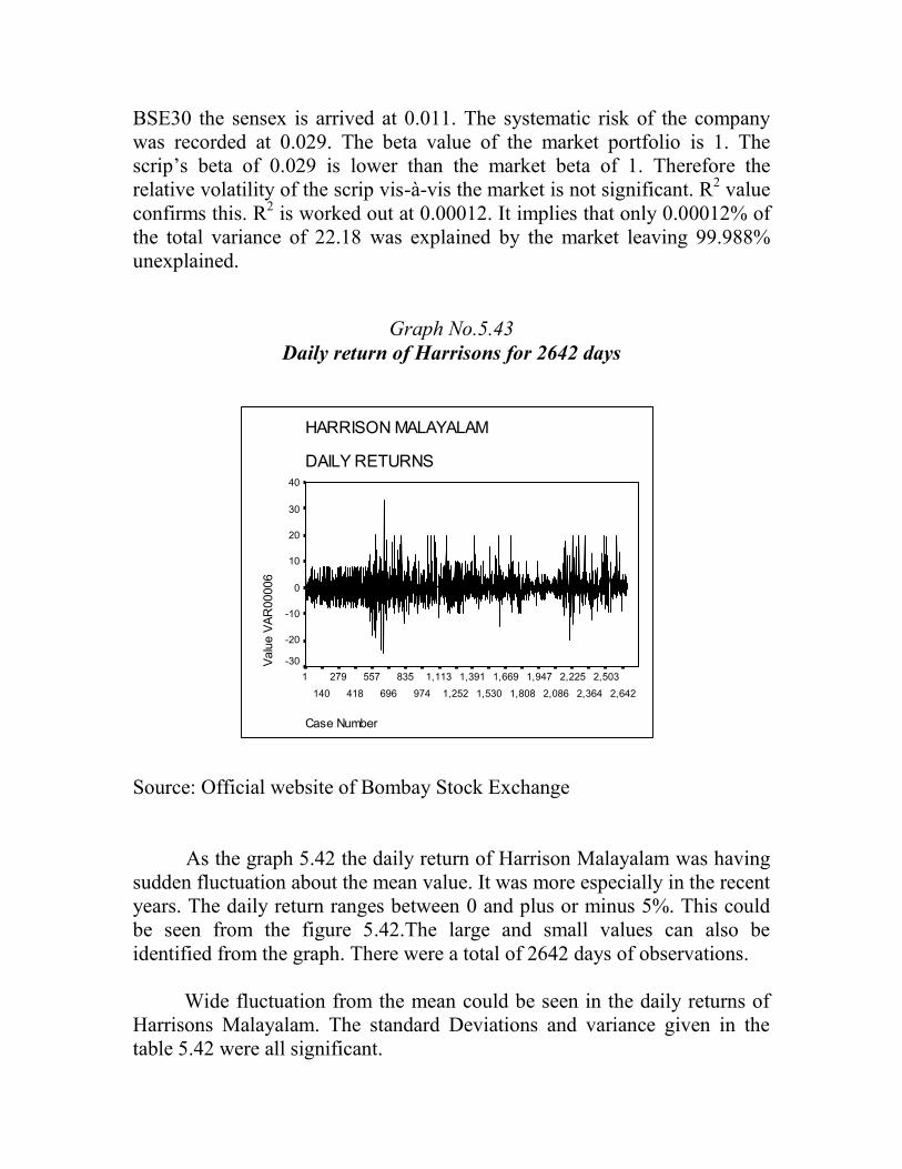
BSE30 the sensex is arrived at 0.011. The systematic risk of the companywas recorded at 0.029. The beta value of the market portfolio is 1. Thescrip’s beta of 0.029 is lower than the market beta of 1. Therefore therelative volatility of the scrip vis-à-vis the market is not significant. R2 valueconfirms this. R2 is worked out at 0.00012. It implies that only 0.00012% ofthe total variance of 22.18 was explained by the market leaving 99.988%unexplained.

Graph No.5.43Daily return of Harrisons for 2642 days


As the graph 5.42 the daily return of Harrison Malayalam was havingsudden fluctuation about the mean value. It was more especially in the recentyears. The daily return ranges between 0 and plus or minus 5%. This couldbe seen from the figure 5.42.The large and small values can also beidentified from the graph. There were a total of 2642 days of observations.

Wide fluctuation from the mean could be seen in the daily returns ofHarrisons Malayalam. The standard Deviations and variance given in thetable 5.42 were all significant.

HARRISON MALAYALAM

DAILY RETURNS

Case Number

2,642

2,503

2,364

2,225

2,086

1,947

1,808

1,669

1,530

1,391

1,252

1,113

974

835

696

557

418

279

140

1

Valu

e VA

R00

006

40

30

20

10

0

-10

-20

-30

Table No.5.44Holding period yield of Harrisons Malayalam for the period 1999-2009

YEAR OP CL HPR HPY1999 36.45 26.5 0.73 -272000 27.1 14.75 0.54 -462001 15.25 14.75 0.97 -32002 15.25 7.05 0.46 -542003 6.7 13.65 2.04 1042004 13.55 62.35 4.6 3602005 64.75 101.15 1.56 562006 103.75 86.15 0.83 -172007 85.95 118.5 1.38 382008 132.95 39.2 0.29 -712009 40.6 134.4 3.31 231

AM 51.91


The table 5.43 above describes the Holding period yield ofHarrison Malayalam. In 1999 the HPY obtained by the firm was -27%. In2009 it was 231%. The increase in HPY was 9.5 since 1999. The lowestHPY was -71 in 2008. The highest was 360% in 2004. In 6 years thecompany earned negative returns. The remaining 4 years the company madepositive HPY. The overall HPY for the entire period was 51.91%.

In the first three years the holding period yield of the stock was allnegative. But the expected HPY was 51.91%. The variability was amazing.Similarly, the highest yield obtained in 2004 was 306% while the expectedwas only 51.91%. In this way wide variability could be identified betweenthe actual and the expected. It all amounted to the high volatility in theactual yield of Harrisons Malayalam.

Graph No.5.44Holding Period Yield of Harrisons Malayalam for the period 1999-2009


The Graph No.5.43 also depicted the same. The HPY in the years2002-2004 formed a peak. The highest HPY in 2004 can be identified as thepeak point. The two peaks above the X-axis represented the positive return.All the other part of the line was below the X-axis.

As per the graph, the HPY for the period shows high volatility. Thedifference between the actual yield obtained and the expected found largelydifferent. Therefore the HPY was found to be uncertain and chaotic. Themajor peak shown in the figure in 2004 was quite unexpected and accidentalwas clear evidence of the presence of high degree of volatility. There weresmall peaks and major and minor troughs shown by the graph. They allrepresented the presence of high volatility in the yield obtained by the stockduring the period.

VAR00003

2009.002008.00

2007.002006.00

2005.002004.00

2003.002002.00

2001.002000.00

1999.00

Mea

n VA

R00

007

400

300

200

100

0

-100

Table No.5.45Annual return of Harrisons Malayalam for the period 1999-2009

Year Return1999 -0.062000 -0.172001 -0.122002 0.452003 0.682004 0.172005 -0.012006 -0.012007 0.232008 -0.342009 0.58

AM 0.13


The table 5.44 the behavior of the average annual return of thecompany was also the same. In 1999 the annual return was -0.06%. In 2009it was 0.58%.The highest annual return was recorded at 0.68% in 2003. Thelowest was recorded at -0.34% in 2008. In 6 years the company facednegative annual returns while in 4 years it made positive annual returns. Theaverage for the 10 year period was 0.13%.

In the first three years the annual returns obtained were all negative.The expected annual returns worked out were 0.13%. There wasconsiderable gap between the expected and the actual. Similarly, widedifference could be noted in the case of smallest annual return and theexpected value. The largest annual returns obtained were 0.68% against theexpected value of 0.13%. The smallest return achieved was -0.34against theexpected 0.13%. What was found from the table was that the existence ofwide variability between the expected and the actual.

Graph No.5.45Annual returns of Harrisons Malayalam for the period 1999-2009


As per the graph 5.44 the annual return of the companyHarrisons Malayalam in the year 2003 and 2004 were very highrepresented in the figure by peak. In 2008 the annual return almosttouched the abscissa. It was the lowest return point for the period. Themovement of the annual return line was very fluctuating andtumultuous.

It was because of the variability between the actual returnsobtained and expected; the curve of annual returns was making such atwists and turns in its way. One major peak and trough were mainlyfound in the graph. It shows the existence high degree of volatility inthe annual returns of the company.

VAR00003

2009.002008.00

2007.002006.00

2005.002004.00

2003.002002.00

2001.002000.00

1999.00

Mea

n VA

R00

008

.8

.6

.4

.2

0.0

-.2

-.4

16. HINDALCO

Table No.5.46Summary statistics of Hindalco from 1999 to 2009


The table 5.45 provides a summary statistics of the performance ofHindalco for the period 1999-2009. The scrip earned an average return of0.05% during the period. It is less than the market average of 0.11%. Theholding period yield worked out for the company is 21.27% which is theexpected rate of return of the company. The company’s performance islower than the expected. The firm’s HPY 21.27 was much better than themarket average of 0.11%. The largest daily return of the firm was registeredas 18.4% whereas the smallest was recorded as -89.78%. The quantitativedifference between the large and small comes to 108.18. It shows widedispersion of return from the expected value. Therefore the variability inreturns is very great in the case of Hindalco during the period. The same istold by the statistic standard deviation with a value of 3.32 and a variance of11.05. Both the standard deviation and variance are significant. Thedistribution of the company’s earnings is not symmetrical. A skewness withvalue of -7.03 signals high level negative grouping and hunchness to the leftside of the mean value. The distribution is also having an enormous level ofpeakness of leptokurtic nature to the tune of 194.2. The kurtosis isleptokurtic since the coefficient is more than 3. The sensex and the scripmove together to the tune of -0.113. The coefficient of covariance -0.113 issignificant. Correlation coefficient which measures the interdependencebetween the scrip and the BSE30 the sensex is arrived at -0.019. Thesystematic risk of the company was recorded at -0.0353. The beta value of

Average return 0.05% Skewness -7.04σ 3.32 Variance 11.05L 18.4 cov -0.113S -89.78 kurtosis 194.2Range 108.18 cor. -0.019Beta -0.0353 HPY 21.27R2 0.000361 Market return 0.11%

the market portfolio is 1. The scrip’s beta of -0.0353 is lower than themarket beta of 1. Therefore the relative volatility of the scrip vis-à-vis themarket is not significant. R2 value confirms this. R2 is worked out at0.000361. It implies that only 0.00036% of the total variance of 11.05 wasexplained by the market leaving 99.964% unexplained.

Graph No.5.46Daily return of Hindalco for 2642 days


The Graph No.5.45 shows the behavior of the daily stock return of theHindalco. The daily returns were thinly spread on the zero line within arange of 0-5%±. There were lot of minor variations on either side of theabscissa. The largest return was registered on the 1669 days’ observationsince 1999. The return was negatively skewed. The fluctuation in the returnfrom the stock cannot be considered violent.

As per table No.5.45 the standard deviation and variance in the dailyreturns were given. From the graph above, it could be understood that theywere all important. The deviations found above and around the mean wasabove 3σ was significant. The minor variations from the mean returns werefound with the daily returns.

HINDALCO

DAILY RETURNS

Case Number

2,642

2,503

2,364

2,225

2,086

1,947

1,808

1,669

1,530

1,391

1,252

1,113

974

835

696

557

418

279

140

1

Valu

e VA

R00

005

40

20

0

-20

-40

-60

-80

-100

Table 5.47Holding period yield of Hindalco for the period 1999-2009

YEAR OP CL HPR HPY1999 517.25 805 1.56 562000 867 737.75 0.85 -152001 741.7 639.8 0.86 -142002 632.6 586.35 0.93 -72003 585.45 1408.3 2.41 1412004 1400.9 1426.8 1.02 22005 1442.85 143.4 0.1 -902006 146.05 174.1 1.19 192007 177.9 214.85 1.21 212008 215.4 51.65 0.24 -762009 54.2 160.75 2.97 197

AM 21.27


The table 5.46 shows the holding period yield of Hindalco for theperiod 1999-2009. In the year 1999 the HPY was 56%. In 2009 it was 197%.HPY increased during this period by 3.5 times. The largest value of HPYwas earned in 2009 itself. The amount of it was 197%. The lowest HPY was-90% in 2005. In 5 years Hindalco earned negative yields. The underlyingtrend of the HPY was to increase. The average HPY for the entire periodunder study was 21.27%.

The actual holding period yield achieved by the scrip wasconsiderably different from the expected whether it was positive or negative.The highest HPY achieved was 197% against the expected 21.27%. Note thedifference between the expected and actual. The difference was 175.73%.Volatility was there to the extent of 175.73% from the expected value.Similarly, the smallest HPY was -90% against the expected 21.27%. Thatmeant a difference of the actual from the expected to the tune of 111.27%. Inthis way there was wide volatility in the HPY of the stock.

Graph No.5.47Holding Period Yield of HINDALCO for the period 1999-2009


The graph 5.46 depicts the behavior of the HPY pictorially. The HPLline starts from the Y-axis and fall. Then rise to make a peak in 2003. Thenit falls steeply cutting the abscissa. There are many peaks and troughs in thepicture. They all show the rough and tough movement of the HPY linebefore it settles at a top point in 2009.

The wide variability expressed by the table was shown in the graph.The line of HPY was found varying from the expected in the forms of peaksand troughs and twists and turns. This behavior of the curve depicted theexistence of high degree of volatility in the holding period yield of the stock.

VAR00003

2009.002008.00

2007.002006.00

2005.002004.00

2003.002002.00

2001.002000.00

1999.00

Mea

n V

AR

0000

4

300

200

100

0

-100

-200

Table No.5.48Annual return of Hindalco for the period 1999-2009


The table 5.47 above shows the annual return of Hindalco for theperiod under study. In 1999 the annual return recorded was 0.25%. In 2009it was 0.53%. The annual return increased during this period by 2.12 times.The highest return was recorded as 0.53% which achieved in 2009 itself.The lowest -0.46% was occurred in 2008. Negative annual returns wereobtained in 5years. The overall average annual return for the entire periodunder study was 0.05%.

The actual annual returns obtained by the stock over years wereshown in the table were far different from the expected 0.05%. See thedifference between 0.53% the highest return against the expected 0.05%.High variability was found. In the same way the annual returns of every yearwere entirely different from the expected. In all these cases wide volatilitywere found.

Year Return1999 0.252000 -0.012001 -0.032002 -0.022003 0.362004 0.042005 -0.342006 0.122007 0.112008 -0.462009 0.53

AM 0.05

Graph No.5.48Annual return of Hindalco for the period 1999-2009


The behavior of annual average return for the period under study ofHindalco is shown in the graph 5.47 above. The annual return during theperiod was highly fluctuating. There is a major peak formation and two deeptroughs during the period. The troughs were highly damaging to the overallperformance of the annual returns. It adversely affected the average annualreturns for the entire period. The recent trough was the lowest average point.

The variability in the annual returns was already located from thetable. It could be seen in the graph also. The curve had violent fluctuationsfrom the expected value. The curve went berserk in many years. Sometimeseven below zero regardless of the expected. It all showed the existence ofhigh degree of volatility in the annual returns.

VAR00003

2009.002008.00

2007.002006.00

2005.002004.00

2003.002002.00

2001.002000.00

1999.00

Mea

n V

AR

0000

5

.6

.4

.2

-.0

-.2

-.4

-.6

17. INDIAN HOTELS

Table No.5.49Summary statistics of Indian Hotels from 1992 to 2001


The table 5.48 provides a summary statistics of the performance ofIndian Hotels for the period 1999-2009. The scrip earned an average returnof 0.04% during the period. It is more than the market average of 0.11%.The holding period yield worked out for the company is 14% which is theexpected rate of return of the company. The company’s performance islower than the expected. The firm’s HPY 14% was much better than themarket average of 0.11%. The largest daily return of the firm was registeredas 16.07% whereas the smallest was recorded as -89.72%. The quantitativedifference between the large and small comes to 105.79. It shows widedispersion of return from the expected value. Therefore the variability inreturns is very high in the case of Indian Hotels during the period. The sameis revealed by the statistic standard deviation with a value of 3.09 and avariance of 9.57. Both the standard deviation and variance are significant.The distribution of the company’s earnings is not symmetrical. skewnesswith value of -8.8 signals high level negative grouping and hunchness to theleft side of the mean. The distribution is also having an enormous level ofpeakness of leptokurtic nature to the tune of 259.6. The kurtosis isleptokurtic since the coefficient is more than 3. The sensex and the scripmove together to the tune of 0.262. The coefficient of covariance 0.262 issignificant. Correlation coefficient which measures the interdependencebetween the scrip and the BSE30 the sensex is arrived at 0.047. The

Average return 0.04% Skewness -8.8σ 3.9 Variance 9.6

L 16.07 cov 0.262S -89.72 kurtosis 259.6Range 105.79 cor. 0.047Beta 0.082 HPY 14%R2 0.0022 Market return 0.11%

systematic risk of the company was recorded at 0.082. The beta value of themarket portfolio is 1. The scrip’s beta of 0.082 is lower than the market betaof 1. Therefore the relative volatility of the scrip vis-à-vis the market is notsignificant. R2 value confirms this. R2 is worked out at 0.0022. It implies thatonly 0.22% of the total variance of 9.6 was explained by the market leaving99.78% unexplained.

Graph No.5.49Daily return of Indian Hotels for 2642 days


Graph 5.48 depicts the behavior of the daily return of the scrip ofIndian Hotels for the period under study. The returns of 2642 days werespread thinly over the zero line with minor fluctuation on either side. Thelowest value of return occurred is seen on 1947th day.’ The return was spreadabout the expected value within a range of 0-5%±.

Even if the daily returns were spread within a range of 0-5% itshowed significant variability. The standard deviation was given as 3.9. Thestandard deviation above 3 is significant.

INDIAN HOTELS

DAILY RETURNS

Case Number

2,642

2,503

2,364

2,225

2,086

1,947

1,808

1,669

1,530

1,391

1,252

1,113

974

835

696

557

418

279

140

1

Val

ue V

AR

0000

3

40

20

0

-20

-40

-60

-80

-100

Table No.5.50Holding period yield of Indian hotels for the period 1999-2009

YEAR OP CL HPR HPY1999 356.25 317 0.89 -112000 333 235.3 0.71 -292001 247.95 155.45 0.63 -372002 157.85 189.65 1.2 202003 187.15 448.25 2.4 1402004 444.85 539.4 1.21 212005 541.45 988.05 1.82 822006 987.75 154.25 0.16 -842007 157.15 159.55 1.02 22008 174.3 45.05 0.26 -742009 45.6 102.35 2.24 124

AM 14


The table 5.49 shows the holding period yield of the scrip Indianhotels. In 1999 the HPY of the firm was -11%. In 2009 it was 124%. TheHPY had been increased during the period by 12.3 times. The lowest returnrecorded during this period was -84 in the year 2006. The highest returnrecorded was 140% in 2003. In 5 years the stock was recorded negativeHPY. The overall HPY for the entire period was 14%.

The variability from the expected HPY of the actual obtained wassignificant. There was wide variability in yields. There was variabilitybetween the HPY of 1999 and the expected to the extent of (14--11) i.e.,25%. In 2009 also the difference was (124-14) ie., 110%. In this way widevariability in yield was found showing high volatility.

Graph No.50Holding Period Yield of Indian Hotels for the period 1999-2009


The graph 5.49 shows the erratic behavior of the stock of IndianHotels. The holding period return never was stable for the scrip. The returnwas highly volatile. In the graph, the HPY line starts from the Y axis from apoint below zero. Then it goes to a peak point in the year 2003. Then itsuddenly fell down and bottomed out before touching zero in 2004. HPYagain rises to another peak and falls severely. In this way the graph shows anumber of peaks and troughs in the movement of the HPY line. The highestreturn was obtained by the scrip in 2004 and the lowest in 2006. These areapparent from the graph.

Because of the variability between the actual HPY and expected therewas high degree of volatility in the yield. The volatility in yield could betraced from the graph. The erratic behavior of the yield curve was due to thisvariability.

VAR00003

2009.002008.00

2007.002006.00

2005.002004.00

2003.002002.00

2001.002000.00

1999.00

Mea

n VA

R00

004

200

100

0

-100

Table No.5.51Annual return of Indian Hotels for the period 1999-2009

Year Return1999 0.022000 -0.092001 -0.152002 0.092003 0.372004 0.102005 0.252006 -0.142007 0.062008 -0.492009 0.39

AM 0.04


The table 5.50 above shows the behavior of annual return made by thestock Indian hotels during the period 1999-2009. In 1999 the annual returnwas 0.02%. In 2009 it was 0.39%. The annual return during this period hadbeen increased by 19.5 times. The lowest annual return was -0.49 in 2008.The highest was 0.39% in 2009. Four years the company made negativereturns. Six years it made positive annual returns. The overall return for theentire period was 0.04%.

The annual returns shown in the table above had high fluctuations.The annual returns of 1999 were 0.02% against the expected rate of 0.04%.In the year 2009 it was 0.39% against the expected value of 0.04% ie., adifference of 0.35%. The variability was very high. In 2000 the actual was -0.09% against the expected 0.04% ie., 0.13% difference. In this way thevariability was there for all years’ annual returns.

Graph No.5.51Annual return of Indian Hotels for the period 1999-2009


The graph 5.50 shows the behavior of the annual return of Indianhotels. The line which shows the annual returns starts from immediatelyafter the zero point in the Y-axis. There were wide fluctuations in themovement of the line. Three peaks and four troughs were formed. The fourthtrough is the lowest annual return point. The underlying trend of the line isto stay high.

The peaks and troughs found in the graph were due to the variabilityin the annual returns. The actual were different from the expected. This waswhat the volatility. This leads to uncertainty and chaos in the minds of thestock holders. Such stocks’ return could not be predicted with accuracy. Thiswill entail lot of difficulties to the investors. The graph shown above revealshigh degree of volatility in the annual returns of the stock

VAR00003

2009.002008.00

2007.002006.00

2005.002004.00

2003.002002.00

2001.002000.00

1999.00

Mea

n V

AR

0000

5

.6

.4

.2

-.0

-.2

-.4

-.6

18. INDIAN REYONS-ADITYA BIRLA NUVO

Table No.5.52Summary statistics of Indian Reyons from 1999 to 2009


The table 5.51 provides a summary statistics of the performance ofAditya Birla Nuvo (Indian Reyon) for the period 1999-2009. The scripearned an average return of 0.13% during the period. It is more than themarket average of 0.11%. The holding period yield worked out for thecompany is 36.82% which is the expected rate of return of the company. Thecompany’s performance is lower than the expected. The firm’s HPY 36.82%was much better than the market average of 0.11%. The largest daily returnof the firm was registered as 20.48% whereas the smallest was recorded as -56.6%. The quantitative difference between the large and small comes to75.2. It shows wide dispersion of return from the expected value. Thereforethe variability in returns is very great in the case of Indian Reyons during theperiod. The same is implied by the statistic standard deviation with a valueof 3.22 and a variance of 10.4. Both the standard deviation and variance aresignificant. The distribution of the company’s earnings is not symmetrical. Askewness with value of -1.5 signals high level of negative grouping andhunchness to the left side to the mean value. The distribution is also havingan enormous level of peakness of leptokurtic nature to the tune of 37.2. Thekurtosis is leptokurtic since the coefficient is more than 3. The sensex andthe scrip move together to the tune of 3.14. The coefficient of covariance3.14 is significant. Correlation coefficient which measures theinterdependence between the scrip and the BSE30 the sensex is arrived at0.005. The systematic risk of the company was recorded at 0.009. The beta

Average return 0.13% Skewness -1.5σ 3.23 Variance 10.4L 18.6 0.029S -56.6 kurtosis 37.2Range 75.2 cor. 0.005Beta 0.009 HPY 36.82R2 0.00003 Market return 0.11%

value of the market portfolio is 1. The scrip’s beta of 0.009 is lower than themarket beta of 1. Therefore the relative volatility of the scrip vis-à-vis themarket is not significant. R2 value confirms this. R2 is worked out at0.00003. It implies that only 0.003% of the total variance of 10.4 wasexplained by the market leaving 99.997% unexplained.

Graph No.5.52Daily return of Indian Reyons for 2642 days

Indian Reyons

Daily Returns

No.of observation

Case Number

2,7182,575

2,4322,289

2,1462,003

1,8601,717

1,5741,431

1,2881,145

1,002859

716573

430287

1441

Value

VAR

0000

2

40

20

0

-20

-40

-60

-80


The graph 5.51 above shows the behavior of daily returns of IndianReyons. The daily returns were spread on the zero line thickly either sidethroghout the length. The largest value is plotted in between 1st and 287th

observation. The deviations from the mean returns were found within therange of 0-5% positive or negative. The deviations were significant. The σabove 3 is significant. Here for the company the σ is 3.23. Thereforedeviations were significant.

Table No.5.53Holding period yield of Indian Reyons for the period 1999-2009

YEAR OP CL HPR HPY1999 113.8 115.65 1.02 22000 124.85 84 0.67 -332001 91.4 72.65 0.79 -212002 70.9 94.05 1.33 332003 93 270 2.9 1902004 270.05 388.25 1.44 442005 392.35 667.2 1.7 702006 676.95 1247.5 1.84 842007 1281.5 2017.25 1.57 572008 2028.05 574.65 0.28 -722009 579.05 876.3 1.51 51

AM 36.82


The table 5.52 shows the behavior of the holding period yield ofIndian Reyons. The HPY in 1999 was 2%. In 2009 it was 51%. The HPYduring this period had been increased by 25.5 times. The lowest HPY wasrecorded as -72 in 2008. The highest was recorded as 190% in 2003. In threeyears the HPY was negative. In seven years the HPY was positive. Theaverage HPY for the entire period was 36.82%.

See the difference between the actual and expected in 1999. Theactual was 2% against the expected 36.82%. The actual was short of34.82%. In 2003 the actual was 190% against the expected 36.82%. Thedifference was whopping 153.18%. High variability can be found with theHPY. In 2009 the actual was 51% against the expected 36.82%. Thedifference was 14.48%. In this way variability of return was there in theholding period yield of the scrip. This shows high degree of volatility in theyield of the stock.

Graph No.5.53Holding Period Yield of Indian Reyons for the period 1999-2009


Graph 5.52 shows the behavior of the HPY of Indian Reyons. TheHPY line shows lot of fluctuations. There were one peak and two troughs inthe movement of the HPY line. The lowest return occurred in 2008 can belocated from the graph. The highest HPY can also be readable from thefigure. The ending HPY is visible in the picture.

The variability of yield of the stock was already found from table. Itsgraphical representation of the same shows high degree of fluctuations of theactual HPY line. It was going ups and downs above and below of theexpected value. Accordingly peaks and troughs were formed. They all showthe extreme form volatility in yields. The yields obtained were not stable andconsistent with the expected value. As there exists wide difference betweenthe actual and expected volatility was said to prevail for the stock. Volatilityof high degree was found with the HPY of the stock

VAR00003

2009.002008.00

2007.002006.00

2005.002004.00

2003.002002.00

2001.002000.00

1999.00

Mea

n V

AR

0000

4

300

200

100

0

-100

Table No.5.54Annual return of Indian Reyons for the period 1999-2009

Year Return1999 0.242000 -0.102001 -0.072002 0.142003 0.462004 0.192005 0.242006 0.282007 0.222008 -0.432009 0.23

AM 0.13


The table 5.53 shows the behavior of annual returns of Indian Reyons.In 1999 the annual return was 0.24%. In 2009 it was 0.23%. The annualreturns of the company for the period were reduced by 4%. The lowestreturn struck for the period was -0.43% in 2008. The highest annual returnthe company achieved was 0.46% in 2003. Three years the company couldmake only negative returns. Indian Reyons made positive annual returns in 7years. The overall trend was to make positive return. The average for theentire period was 0.13%.

As shown by the table there was high degree of variability of returns.The difference between the expected value and actual was significant. Takethe case of the year 2009. The actual for the year was 0.23% against theexpected return of 0.13%. The actual varies to the extent of 0.10%. In 1999the actual annual return was 0.24% against the expected value of 0.13%. Thedifference was 0.11%. In this way there were wide variability in annualreturns of the company.

Graph No.5.54Annual return of Indian Reyons for the period 1999-2009


From the graph 5.53 it could be discerned that the annual return linestarts at 0.24% return point from the Y-axis. It falls down during 2000 to -0.10%. In 2003 it rises from there and went to 0.07%. It again rose to 0.14%in 20002.In 2003 it reached the topmost return point of 0.46% for the periodin 2004. In 2005 it fell down to 0.24%. In 2008 the line deeply fell to thelowest return point of -.43% for the period and bottomed out to raise to settleat 0.23% in 2009. The return increased and decreased frequently and thescrip faced frequent upheavals and violent fluctuations throughout the 10year period. In spite of it, the overall trend of the annual return was to stayincreased. In majority of years the company earned return below zero-line.Only in few years it earned better. But in 1999 the return formed a peakwhich caused the overall rate of 0.048%.

Due to the variability in returns the graph shows wide volatility inreturns of the company. Accordingly, the annual returns line goes ups anddowns crossing the average line.

VAR00003

2009.00

2008.00

2007.00

2006.00

2005.00

2004.00

2003.00

2002.00

2001.00

2000.00

1999.00

Mea

n VA

R00

005

.6

.4

.2

-.0

-.2

-.4

-.6

19. ITC Ltd

Table No.5.55Summary statistics of ITC from 1999 to 2009


The table 5.54 provides a summary statistics of the performance ofITC Ltd for the period 1999-2009. The scrip earned an average return of0.05% during the period. It is less than the market average of 0.11%. Theholding period yield worked out for the company is 4.27% which is theexpected rate of return of the company. The company’s performance ishigher than the expected. The firm’s HPY 4.27% was not up to theperformance of the market average 0.11%. The HPY was lower than themarket return. The largest daily return of the firm was registered as 11.08%whereas the smallest was recorded as -92.74%. The quantitative differencebetween the large small comes to 103.82. It shows wide dispersion of returnfrom the expected value. Therefore the variability in returns is very great inthe case of ITC Ltd during the period. The same is confirmed by thestatistics standard deviation with a value of 2.93 and a variance of 8.58. Boththe standard deviation and variance are significant. The distribution of thecompany’s earnings is not symmetrical. A skewness with value of -11.3signals high level negative grouping and hunchness left to the mean. Thedistribution is also having an enormous level of peakness of leptokurticnature to the tune of 363.19. The kurtosis is leptokurtic since the coefficientis more than 3. The sensex and the scrip move together to the tune of acovariane of -0.016. The coefficient of covariance -0.016 is significant.Correlation coefficient which measures the interdependence between thescrip and the BSE30 the sensex is arrived at -0.003. The systematic risk of

Average return 0.05% Skewness -11.3σ 2.93 Variance 8.58L 11.08% cov -0.016S -92.74% kurtosis 363.19Range 103.82 cor. -0.003Beta -0.005 HPY 4.27R2 0.000009 Market return 0.11%

the company was recorded at -0.005 The beta value of the market portfoliois 1. The scrip’s beta of -0.005 is considerably lower than the market beta of1. Therefore the relative volatility of the scrip vis-à-vis the market is notsignificant. R2 value confirms this. R2 is worked out at 0.000009. It impliesthat only 0.0009% of the total variance of 8.58 was explained by the marketleaving 99.99% unexplained.

Graph No.5.55Daily return of ITC for 2642 days


The Graph 5.54 shows the behavior of the daily return of ITC Ltd forthe study period. It can be seen from the figure that the returns were thicklypacked along the line X-axis. The returns were spread to either side of thezero line with a margin of 0—5%±. The lowest return is shown in the graphby a narrow line as hanging from the zero line towards the bottom line at1669th observation. The largest value can also be readable from the graph.

ITC

DAILY RETURNS

Case Number

2,642

2,503

2,364

2,225

2,086

1,947

1,808

1,669

1,530

1,391

1,252

1,113

974

835

696

557

418

279

140

1

Valu

e VA

R00

002

20

0

-20

-40

-60

-80

-100

Table No.5.56Holding period yield of ITC Ltd for the period 1999-2009

YEAR OP CL HPR HPY1999 754 665 0.88 -122000 718.15 896.6 1.25 252001 896.05 676.8 0.76 -242002 683.9 660.4 0.97 -32003 658.9 984.55 1.49 492004 992.05 1309.8 1.32 322005 1313.05 142 0.11 -892006 140.55 175.95 1.25 252007 176.85 210.3 1.19 192008 217.6 171.45 0.79 -212009 171.4 250.85 1.46 46

AM 4.27


The table 5.55 shows the character of the holding period yield ofITC Ltd. In 1999 the HPY was -12%. In 2009 it was 46%. The yield duringthis period was increased by 4.8 times. The lowest yield sustained by ITCwas -89% in 2005. The highest yield was struck at 49% in 2003. Over 5years the scrip succumbed to negative returns. The other 5 years positiveyield were gained. The yield was not steady and stable. Fluctuations werefound most frequently in alternating years. Despite it, the overall trend wasto go on increase in the HPY.

The average holding period yield was 4.27%. In 1999 the actualHPY obtained was -12% against the expected 4.27. The variability was tothe extent of 16.47%. In 2009 the actual HPY was 46% against the expectedvalue of 4.27 ie.,a difference of 41.73%. There was volatility in the HPY ofthe stock.

Graph No.5.56Holding period yield of ITC Ltd for the period 1999-2009


As shown by the graph 5.55 the HPY line goes through all the roughand tough ways to reach the year 2009 from 1999. The scrip confrontedthree falls, of them one was major and 3 peaks. The largest yield wasmarked in 2003 above 40% return level. The lowest level of yield was struckin 2005 below -80% yield point. The trend of the line was to go upwards.

The actual HPY line shown by the graph had high volatility. Itrepresents high variability between the actual and expected values. While theexpected HPY was 4.27% in 2005 the actual HPY was -89%; a variability of93.27%. The trough in the year 2005 was owing to this variability in HPY. Itshows the fact that there was wide variability between the expected andactual values of HPY.

VAR00003

2009.002008.00

2007.002006.00

2005.002004.00

2003.002002.00

2001.002000.00

1999.00

Mea

n V

AR

0000

4

60

40

20

0

-20

-40

-60

-80

-100

Table No.5.57Annual return of ITC Ltd for the period 1999-2009

Year Return1999 0.022000 0.152001 -0.082002 0.002003 0.172004 0.132005 -0.202006 0.122007 0.102008 -0.062009 0.18

AM 0.05


The annual return based on the daily returns for the period from 1999to 2009 was furnished in the table 5.56. As per it in 1999 the annual returnwas 0.02%. In 2009 it was 0.18%. In the meantime the return had beenincreased by 9 times. The lowest annual return was noted at -0.20% in 2005.The highest annual return was recorded at 0.18% in 2009. Over 3 years thescrip ITC confronted negative annual returns. The remaining 7 years thefirm made positive returns. In 2000 no annual return was recorded. Onaverage the company managed to secure an annual return of 0.05%.

The expected value of annual return was 0.05%. The stock had notearned this expected value or a return near to this in any year. All the actualreturns were far away from the expected value. In 1999 the actual returnsearned were 0.02% against the expected 0.05%.The actual varies from theexpected to the extent of 0.03%. In 2009 the actual earned was 0.18%against the expected 0.05%. A variation of 0.13%. In 2005 the actual was -0.2% against the expected 0.05%. A variation of -0.25%. In this way theannual returns show high level of variability.

Graph No.5.57Annual returns of ITC Ltd for the period 1999-2009


As explained above the highly fluctuating line of annual returncan be seen from the graph 5.56. The annual return starts from justimmediately above the zero % point on Y-axis. There from it can beseen on the table that the return makes twists and turns year after yearresulting in violent ups and downs on a straight line before it settles ata comfortable positive return in 2009. In the meantime the scrip faces3 major downswings and 4 upswings. The second downswing led tolowest annual return for the period under study in the year 2005. Theupswings all were resulted in heights which were all more or lessidentical. The still higher annual return where the line settled was theone in 2009. It can be said that the upswing has slight edge over thedownswing.

As per the graph, the volatility of the annual returns was veryhigh due to overwhelming variability in returns. The expected andactual returns were not consistent over period. Due to this fact therewere too much chaos and uncertainty prevailing over.

VAR00003

2009.002008.00

2007.002006.00

2005.002004.00

2003.002002.00

2001.002000.00

1999.00

Mea

n V

AR

0000

5

.3

.2

.1

-.0

-.1

-.2

-.3

20. AXIS BANK

Table No.5.58Summary statistics of Axis Bank from 1999 to 2009


The table 5.57 provides a summary statistics of the performance ofAxis Bank for the period 1999-2009. The scrip earned an average return of0.2% during the period. It is more than the market average of 0.11%. Theholding period yield worked out for the company is 60.09% which is theexpected rate of return of the company. The company’s performance islower than the expected. The firm’s HPY 60.09% was overwhelminglyhigher than the market average of 0.11%. The largest daily return of the firmwas registered at 24.86% whereas the smallest was recorded as -16.37%.The quantitative difference between the large and small comes to 41.23. Itshows only narrow dispersion of return from the expected value. Thereforethe variability in returns is very low in the case of Axis Bank during theperiod. The same is confirmed by the statistics standard deviation with avalue of 3.4 and a variance of 11.7. Both the standard deviation and varianceare normal. The distribution of the company’s earnings is not symmetrical.A skewness with value of 0.86 signals high level positive grouping andhunchness right to the mean value. The distribution is also having anenormous level of peakness of leptokurtic nature to the tune of 5.07. Thekurtosis is leptokurtic since the coefficient is more than 3. The sensex andthe scrip move together to the tune of 0.607. The coefficient of covariance0.607 is significant. Correlation coefficient which measures theinterdependence between the scrip and the BSE30 the sensex is arrived at0.099. The coefficient is significant at 0.01 level of significance. The

Average return 0.2% Skewness 0.86σ 3.42 Variance 11.7L 24.86% cov 0.607S -16.37% kurtosis 5.07Range 41.23 cor. 0.099Beta 0.19 HPY 60.09%R2 0.01 Market return 0.11%

systematic risk of the company was recorded at 0.19. The beta value of themarket portfolio is 1. The scrip’s beta of 0.19 is lower than the market betaof 1. Therefore the relative volatility of the scrip vis-à-vis the market is notsignificant. R2 value confirms this. R2 is worked out at 0.01. It implies thatonly 1% of the total variance of 11.7 was explained by the market leaving99% unexplained.

Graph No.5.58Daily return of Axis Bank for 2642 days


The graph 5.57 above shows the behavior of daily return of Axis bankfor the period under study. The returns were thickly pasted along the X-axison either side of it. It shows the density of occurrence of returns for the 10year period. Over 2642 days of observation were covered by the graph. Anoverwhelming grouping or hunchness can be observed on the right side ofthe picture. It is an indicator of the presence of high level skewness. Thedistribution of returns was not normal. Most of the values can be foundwithin a range of 0-5%±.The largest and smallest values of returns are alsoplotted in the graph.

AXIS BANK

DAILY RETURNS

Case Number

2,6422,503

2,3642,225

2,0861,947

1,8081,669

1,5301,391

1,2521,113

974835

696557

418279

1401

Valu

e VA

R000

07

30

20

10

0

-10

-20

Table No. 5.59Holding Period Yield of Axis Bank for the period 1999-2009

YEAR OP CL HPR HPY1999 16.35 24 1.47 472000 25.9 45.3 1.75 752001 45.75 26.4 0.58 -422002 26.25 44.8 1.71 712003 43.55 135.15 3.1 2102004 137.2 185.2 1.35 352005 188.95 286.35 1.52 522006 288.3 469.05 1.63 632007 467.45 967.1 2.07 1072008 973 504.65 0.52 -482009 517.25 988.7 1.91 91

AM 60.09


The above table 5.58 shows the behavior of Holding period Yield ofAxis Bank for the period 1999-2009. In 1999 the HPY obtained by the firmwas 47%. In 2009 it was 91%. In the meantime HPY had been increased by1.9 times. The lowest yield secured by the scrip was -48% in 2008. Thehighest yield was 210% in 2003. The company succumbed to negativereturns in 2 years. But scrip managed to earn positive yields over 8 years. Onaverage Axis Bank achieved 60.09% yield over the entire period understudy.

The table depicts the prevalence of variability of yields of high degree.Variability arises since there is difference between the actual yield obtainedand the expected. In the year 1999, the actual yield was 47% whereas theexpected 60.09%. Here the variability was 13.09%. In 2009 it was 30.91%.So there was high variability which causes the high volatility in yields.

Graph No.5.59Holding Period Yield of Axis Bank for the period 1999-2009


The graph 5.58 shows the behavior of the HPY of Axis bank duringthe period 1999-2009. The HPY starts from a point on the Y-axis just abovebut in the middle of 0 and 100%. It moves in a straight line to settle in 2009.In the mean time it comes across 3 troughs and 4 peaks. One of the peakswas major which denoted the largest HPY secured by the scrip lying above200% point in 2003. One of the troughs, rather the last one in 2008 indicatesthe lowest HPY point with nearly -100%. Even though there are 3 falls only2 are below zero line. On the average the holding period yield wasappreciable. But the result was neither steady nor stable. The line of HPYwas highly erratic. Peaks and troughs walk hand in hand. Ups and downsoccur one after another cyclically and alternatively. The graph shows highdegree of volatility in yields.

VAR00003

2009.002008.00

2007.002006.00

2005.002004.00

2003.002002.00

2001.002000.00

1999.00

Mea

n V

AR

0000

4

300

200

100

0

-100

Table No. 5.60Annual Returns of Axis Bank for the period 1999-2009

Year Return1999 0.262000 0.292001 -0.172002 0.242003 0.512004 0.192005 0.202006 0.232007 0.332008 -0.152009 0.34

AM 0.21


The table 5.59 above shows the behavior of annual returns of AxisBank during the period 1999-2009. In 1999 the annual return was 0.26%. In2009 it was 0.34%. The annual returns had been increased ever since 1999by 1.3 times. So the annual return of the scrip was growing over years. Thelargest returns were 0.51% which occurred in 2003. On the contrary thesmallest was 0.17% occurred in 2001. The company faced negativereturns over 2 years. Over 8 years the scrip gained positive returns. Onaverage Axis Bank secured 0.21% of annual returns over the entire periodunder study.

The average or expected annual return was 0.21%. The actual returnsearned by the stock in different years were either more or less than theexpected. The excess or short of the returns over the expected returns wasthe variability in the returns. The annual returns shown by the table wasshowing the fact that the annuals were highly volatile

Graph No.5.60Annual Returns of Axis bank for the period 1999-2009


The graph 5.59 shows the behavior of the annual returns of Axis bankduring the period 1999-2009. The Annual returns line starts from a point onthe Y-axis just above the point 0.2%. It moves in a straight line to settle in2009. In the mean time it goes through 3 troughs and 4 peaks. One of thepeaks was major which denoted the largest annual returns secured by thescrip lying above 0.4% scale in 2003. One of the troughs, rather the secondone against the year 2001 along the X-axis indicates the lowest annualreturns just below 0.2% scale on the Y-axis. Even though there are 3 fallsonly 2 are below zero line. On the average the holding period yield wasappreciable. But the result was neither steady nor stable. The line of annualreturns was highly volatile. Peaks and troughs occur constantly. Ups anddowns come one after another frequently and alternatively. The figure showsthe existence of high degree volatility in the returns.

VAR00003

2009.002008.00

2007.002006.00

2005.002004.00

2003.002002.00

2001.002000.00

1999.00

Mea

n V

AR

0000

5

.6

.4

.2

0.0

-.2

-.4

BSE30 AS MARKET PROXY-SENSEX

Table No.5.61Summary statistics of BSE30 SENSEX from 1999 to 2009


BSE30 had an average return of 0.11%. Its Holding period yield was24.2%. The HPY or the expected return of the BSE30 was greater than itsaverage returns. The standard deviation σ 1.79 was insignificant since1.79<3. Largest daily return was 17.35 and the smallest daily return was -11.1%. The quantitative difference between the large and small values was28.45. This range did not indicate any significant risk. The variance 3.2 wasalso insignificant. It all means the daily returns of all days were more or lessequal to or lying about the mean value of 0.11%. The distribution of returnhad an insignificant amount of positive skewness to the extent of 0.048. Butthe distribution had peakedness or kurtosis to the extent of 5.09. It was aleptokurtic type of peakedness. The variance and covariance were identicalto the BSE30.

Average return 0.11% Skewness 0.048σ 1.79 Variance 3.2L 17.35 cov 3.2S -11.1 kurtosis 5.9Range 28.45 cor. 1.00Beta 1.00R2 1.00 HPY 24.2%

Graph No.5.61Daily Returns of BSE30 for 2642 days.


In the graph above, the daily returns of BSE30 Sensex were plotted. Thedensity of transaction of the market was discernable from the graph. Thereturns of 2642 days were plotted in the graph. These days were the actualmarket days from 1999 to 2009. The average market return for the periodwas given in the table 5.60 as 0.11%. The graph shows that almost all day’sreturns were swarmed about that value. The average return was somewhatnear to the zero. Most of the values could be found within a range of 0—1%.Occasional aberrations were there. The large and small values could belocated from the graph. The deviations were there from the average but theywere insignificant since the standard deviation of the market was below 3σ.The variance too was insignificant. The daily returns were thickly packed oneither side of the zero line. The actual returns of the days would not be faraway from the mean. The individual values were tightly knitted together sothat there would not be much difference between the actual and the meanreturns. A close examination of the graph would reveal the presence somenominal grouping of values on the right hand side of the picture due to thepositive skewness of the distribution of the returns.

DAILY RETURNS

BSE30

NO. OF OBSERVATIONS

Case Number

2,6232,485

2,3472,209

2,0711,933

1,7951,657

1,5191,381

1,2431,105

967829

691553

415277

1391

Valu

e VA

R00

004

20

10

0

-10

-20

Table No.5.62Holding Period Yield of BSE30 for the period 1999-2009

YEAR OP CL HPR HPY1999 3060.34 5005.82 1.64 642000 5375.11 3972.12 0.74 -262001 3955.08 3262.33 0.82 -182002 3246.15 3377.28 1.04 42003 3390.12 5838.96 1.72 722004 5915.47 6602.69 1.12 122005 6679.2 9397.93 1.41 412006 9390.14 13786.91 1.47 472007 13942.24 20286.99 1.46 462008 20300.71 9647.31 0.48 -522009 9903.46 17464.81 1.76 76

AM 24.18182


Table No.5.61 shows the Holding Period Yield of BSE30 for the periodfrom 1999 to 2009. The average HPY for the period was shown as 24.18%.This yield was the expected return of market index. Every year the marketindex expects a holding period value of 24.18%. But the actual yields forvarious years from 1999 to 2009 were given in the table. The table says thatthere is variability of returns from the expected. In 1999 the yield actuallyobtained from the market index was 64% against the expected value of24.18%. In 2009 the yield was 76%. In both cases the actual was well abovethe expected. But in 2000 and 2001, the actual were negatives. The highestactual yield was in 1999 of 76% well above the expectation. The lowestyield was in 2008 of -56%. From 1999 to 2009, the HPY had been increasedby a rate of 19%. In three years the HPY was negative. The year 2008 wasthe most disastrous one for market index. The table says that there is highvariability in yields. The actual yields were different from the expected inalmost all cases. The difference was bigger. The difference will be eitherabove the expected or below the expected. But there was variability ofyields. This variability in yield becomes the cause for volatility. Hence, HPYof the market had high volatility.

Graph No.5.62Holding period Yield of BSE30 for the period 1999-2009


The graph 5.61 above shows the Holding period yield of BSE30 for theperiod 1999-2009. Due to variability in yields already explained the HPYcurve in the graph shows wide volatility. It could be seen from the figure.The curve was going hither and thither, ups and downs, forming peaks andtroughs and also minor erratic vibrations throughout its length before settlingin 2009. It was always uncertain as to which value it would settle. All thevalues settled by the curve will be either above or below the expected value.That is, the realized yield was different from the expected. This is whatvariability in yield. It is also called as volatility. Volatility in yield was thereason for the twist and turn of the curve seemingly directionless. The yieldcurve of the market index was thus found highly volatile.

VAR00001

2009.002008.00

2007.002006.00

2005.002004.00

2003.002002.00

2001.002000.00

1999.00

Mea

n VA

R00

002

100

80

60

40

20

0

-20

-40

-60

Table No.5.63Annual returns of BSE30 for the period 1999-2009

Year Return1999 0.252000 -0.072001 -0.012002 0.092003 0.292004 0.102005 0.172006 0.182007 0.172008 -0.242009 0.27

AM 0.11


The table 5.62 shows the annual returns earned by the market indexfor the period 1999-2009. The annual returns of all years from 1999 to 2009were given in the table. Accordingly in 1999 the annual return was 0.25%.In 2009 the annual return was 0.27%. In 2005 the annual return was 0.17%.In 2008 the annual return was -0.24%. The average of the annual return was(Arithmetic mean) 0.11%. The investors of market index expect every year areturn of 0.11%.

The rate of growth of annual returns from 1999 to 2009 was 8%. Thehighest annual return was recorded as 0.27% in 2009. The lowest was -0.24% in 2008. In three years the annual returns were negative.

The actual annual returns were all having huge difference from theexpected. For example, in 1999 the annual return realized was 0.25% againstthe expected 0.11%. The actual was 0.14% bigger. In 2009 the annual returnwas 0.27% which was 0.19% higher than the expected. In 2008 the actualwas -0.24 which was -0.35% lower than the expected. In this way the annualreturns showed variability in returns. The variability in returns was volatilityin returns cause distress to investors. The annual returns of the BSE30, thus,showed high volatility for the period.

Graph No.5.63Annual returns of BSE30 for the period 1999-2009


The graph 5.62 shows the graphical representation of the annual returns ofBSE30 for the period 1999-2009. As explained under the table earlier, thevariability of returns was very high in the case of BSE30 index. In the graphit could be seen that there were four peaks and three troughs. The peaks andtroughs were values above or below the expected. In the case of peaks theannual returns realized were higher than the expected. In the case of troughsit was lower than the expected. But due to variability in annual return thevolatility of the return curve was very high. The curve was movingerratically in a zigzag way, rising and falling showing signals of uncertaintyand chaos. The annual return line was highly volatile during the period.

VAR00001

2009.002008.00

2007.002006.00

2005.002004.00

2003.002002.00

2001.002000.00

1999.00

Mea

n VA

R00

003

.4

.3

.2

.1

-.0

-.1

-.2

-.3

Table No.5.64Consolidated Summary Statistics for the period 1999-2009

Sl.No Scrip Mean%

σ σ 2 Cov R β Skew kurt

1 ACC 0.09 3.32 11.04 0.15 0.025 0.046 -7.6 2122 Apollo 0.10 3.81 14.54 0.06 0.009 0.02 -4.1 112.95 Asian pai 0.09 2.09 4.35 0.02 0.006 0.007 -2.9 57.93 Arvind 0.07 3.9 14.9 -2.28 -0.33 -0.71 0.77 7.354 Ashok 0.11 3.79 22 -0.034 -0.005 -0.011 -4.5 115.26 Axis Ban 0.21 3.42 11.7 0.607 0.099 0.19 0.86 5.077 Ballarpur 0.08 3.61 13 0.148 0.023 0.046 -3.49 90.418 Castrol 0.02 2.34 5.46 0.025 0.006 0.008 -2.5 71.19 Cent.tex 0.17 3.98 15.8 0.021 0.003 0.01 0.18 2.8210 Cen.Enk 0.12 3.12 9.72 0.371 0.066 0.12 0.53 2.2111 Colgate 0.07 2.06 4.26 0.041 0.011 0.013 0.88 6.4712 Crompton 0.17 3.97 15.78 0.363 0.051 0.113 -2.55 59.2713 Escorts 0.09 3.72 13.80 0.242 0.036 0.0756 0.33 2.5514 Garware 0.17 4.83 23.36 0.311 0.036 0.0973 0.87 4.0815 Gujarat 0.12 3.24 10.52 0.093 0.016 0.029 0.41 2.9716 Harrison 0.16 4.71 22.18 0.093 0.011 0.029 0.69 3.9517 Hindalco 0.05 3.32 11.05 -0.113 -0.019 -0.035 -7.04 194.1818 Indian Ho 0.04 3.09 9.57 0.262 0.047 0.082 -8.8 259.619 Ind.Reyon 0.13 3.23 10.42 0.029 0.005 0.009 -1.5 37.220 ITC 0.05 2.93 8.59 -0.016 -0.003 -0.005 -11.3 363.2

21 BSE30 0.11 1.79 3.2 3.2 1.000 1.000 0.048 5.9Mean 0.10 3.42 12.6 0.02 0.005 0.007 -2.538 80.52


The table 5.64 shows all the statistical tools used in the analysis of thischapter.The consolidated summary statistics provides the information about theposition of the companies for the period 1999-2009. It can be made out fromthe table that no company was making negative average returns during thisperiod. The largest average return 0.21% was earned by Axis Bank. It wasCastrol which made the smallest average return 0.02%. Garware Polyesterhad the highest standard deviation of 4.83. The lowest standard deviation2.06 was of the stock Colgate Palmolive. Garware had the highest variancealso. Colgate had the lowest variance. Covariance of Axis Bank with 0.67was the highest whereas Hindalco with -0.113 had the smallest. Axis bankhad highest correlation 0.099 with the BSE30. Arvind Mills’ correlation -0.33 was the lowest. Axis bank’s beta 0.19 was the highest whereas ArvindMills’-0.71 was the least. Colgate had the highest skewness of 0.88. But

Indian Hotels’ -8.8 was the smallest skewness. Lastly, ITC’s 363.2 was thehighest kurtosis while Century Enka’s 2.21 was the smallest kurtosis.

Table No.5.65Comparison of Actual and Expected Return in percentage

The table No.5.65 shows HPY and average return earned by the scripsduring the study period. A comparison is facilitated by the table. A closescrutiny will reveal that HPY of all companies were higher than their meanreturn for the period. In the right extreme column of the table whether thescrip’s mean return is above or below the HPY is shown. If the stocks meanreturn is below the HPY, the stock is underperforming during the perioddespite its potential. It can be seen that the HPY of all stocks were higherthan their Mean returns.

Sl.No Name of the Stock HPY Mean1 ACC 13 0.09 Below2 Apollo Tyres 24.64 0.10 Below3 Aravind Mills 14.45 0.07 Below4 Ashok Leyland 48.27 0.11 Below5 Asian Paints 23.27 0.09 Below6 Ballarpur Industries 16.64 0.08 Below7 Castrol 4.82 0.02 Below8 Century 53.00 0.17 Below9 Century Enka 51.82 0.12 Below10 Colgate Palmolive 12.91 0.07 Below11 Crompton Greeves 61.91 0.17 Below12 Escorts Ltd. 25.73 0.09 Below13 Garware Polymer 62.73 0.17 Below14 Gujrath Narmada 37.82 0.12 Below15 Harrison Malayalam 51.91 0.16 Below16 Hindalco 21.27 0.05 Below17 Indian Hotels 14 0.04 Below18 Indian Reyons 36.82 0.13 Below19 ITC Badrachalam 4.27 0.05 Below20 Axis Bank 60.09 0.21 Below

Table No.5.66HPY and Mean Return earned by the stocks during 1999-2009

Sl.No Name of the Stock HPY Mean1 Axis Bank 60.09 0.212 Century 53.00 0.173 Crompton Greeves 61.91 0.174 Garware Polymer 62.73 0.175 Harrison Malayalam 51.91 0.166 Indian Reyons 36.82 0.137 Century Enka 51.82 0.128 Gujrath Narmada 37.82 0.129 Ashok Leyland 48.27 0.1110 Apollo Tyres 24.64 0.1011 ACC 13 0.0912 Asian Paints 23.27 0.0913 Escorts Ltd. 25.73 0.0914 Ballarpur Industries 16.64 0.0815 Aravind Mills 14.45 0.0716 Colgate Palmolive 12.91 0.0717 Hindalco 21.27 0.0518 ITC Badrachalam 4.27 0.0519 Indian Hotels 14 0.0420 Castrol 4.82 0.02


The above table 5.66 shows the mean returns earned by the 20 stocksunder study. HPY is also given in the table for facilitating comparison. Asper the table Axis Bank has earned the highest average return to tune of0.21%. The next highest is Century Textiles, Crompton Greaves, andGarware Polyester all with mean return of 0.17%. The lowest in the list isCastrol with a mean return of 0.02%.

Table No.5.67HPY (Holding Period Yield) earned by the stocks 1999-2009

Sl.No Name of the Stock HPY1 Garware Polyester 62.732 Crompton Greaves 61.913 Axis Bank 60.094 Century Textiles 53.005 Harrison Malayalam 51.916 Century Enka 51.827 Ashok Leyland 48.278 Gujarath Narmada 37.829 Indian Reyons (Aditya Birla Nuvo) 36.8210 Escorts Ltd. 25.7311 Apollo Tyres 24.6412 Asian Paints 23.2713 Hindalco 21.2714 Ballarpur Industries 16.6415 Arvind Mills 14.4516 Indian Hotels 1417 ACC 1318 Colgate Palmolive 12.9119 Castrol 4.8220 ITC Ltd 4.27

In the above table 5.67, HPY earned by the 20 stocks weregivien.HPY was shown in per cent. The stocks in the table were placedaccording to the amount of HPY. From the table it can be understood that nostock had earned negative returns during the period. All made only positivereturns.

The stock which is having highest HPY is Garware Polyester. Its HPYwas 62.73.The second to Garware Polyester is Crompton Greaves with aHPY of 61.91. The next highest is Axis Bank with HPY of 60.9. ITC Ltdwas the lowest with HPY of 4.27.

chapter five study of behaviour of equity returns analysis...

Documents