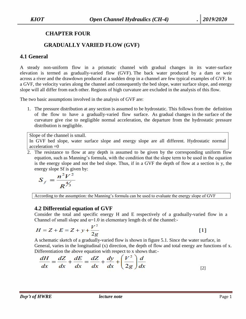
chapter four gradually varied flow (gvf) 4.1 general

KIOT Open Channel Hydraulics (CH-4) . 2019/2020

Dep’t of HWRE lecture note

CHAPTER FOUR

GRADUALLY VARIED FLOW (GVF)

4.1 General

A steady non-uniform flow in a prismatic channel with gradual changes in its water-surface

elevation is termed as gradually-varied flow (GVF). The back water produced by a dam or weir

across a river and the drawdown produced at a sudden drop in a channel are few typical examples of GVF. In

a GVF, the velocity varies along the channel and consequently the bed slope, water surface slope, and energy

slope will all differ from each other. Regions of high curvature are excluded in the analysis of this flow.

The two basic assumptions involved in the analysis of GVF are:

1. The pressure distribution at any section is assumed to be hydrostatic. This follows from the definition

of the flow to have a gradually-varied flow surface. As gradual changes in the surface of the

curvature give rise to negligible normal acceleration, the departure from the hydrostatic pressure

distribution is negligible.

Slope of the channel is small.

In GVF bed slope, water surface slope and energy slope are all different. Hydrostatic normal

acceleration =0

2. The resistance to flow at any depth is assumed to be given by the corresponding uniform flow

equation, such as Manning’s formula, with the condition that the slope term to be used in the equation

is the energy slope and not the bed slope. Thus, if in a GVF the depth of flow at a section is y, the

energy slope Sf is given by:

According to the assumption: the Manning’s formula can be used to evaluate the energy slope of GVF

4.2 Differential equation of GVF Consider the total and specific energy H and E respectively of a gradually-varied flow in a

Channel of small slope and α=1.0 in elementary length dx of the channel:-

A schematic sketch of a gradually-varied flow is shown in figure 5.1. Since the water surface, in

General, varies in the longitudinal (x) direction, the depth of flow and total energy are functions of x.

Differentiation the above equation with respect to x shows that:-

[2]



Figure 4.1 Schematic sketch of GVF

In this equation the meaning of each term is as follows:-

1. Represents the energy slope. Since the total energy of the flow always decreases in the

direction of the motion, it is common to consider the slope of the decreasing energy line as

positive. Denoting it by Sf:-

2. Denotes the bottom slope. It is common to consider the channel slope with bed elevations

decreasing in the downstream direction as positive. Denoting it as So.

3. Represents the water surface slope relative to the bottom of the channel.

This forms the basic differential equation of GVF and is also known as the dynamic equation of GVF. If a

value of the kinetic energy correction factor α greater than unity is to be used,



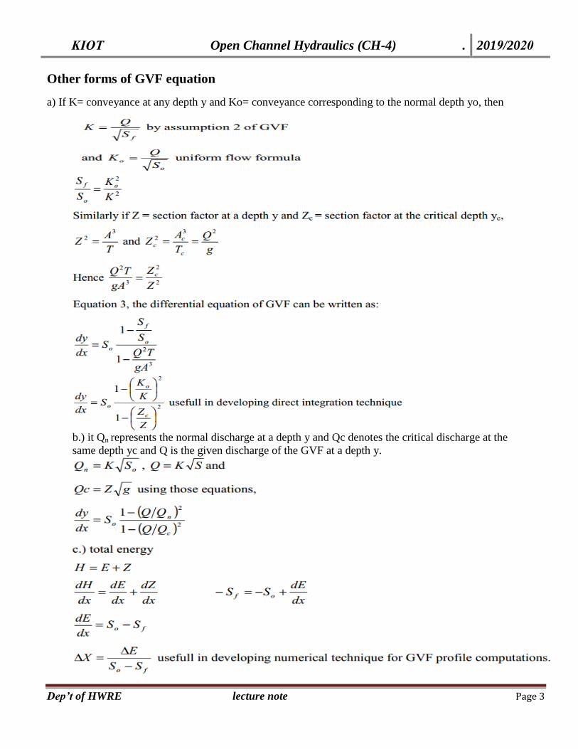
Other forms of GVF equation

a) If K= conveyance at any depth y and Ko= conveyance corresponding to the normal depth yo, then

b.) it Qn represents the normal discharge at a depth y and Qc denotes the critical discharge at the

same depth yc and Q is the given discharge of the GVF at a depth y.



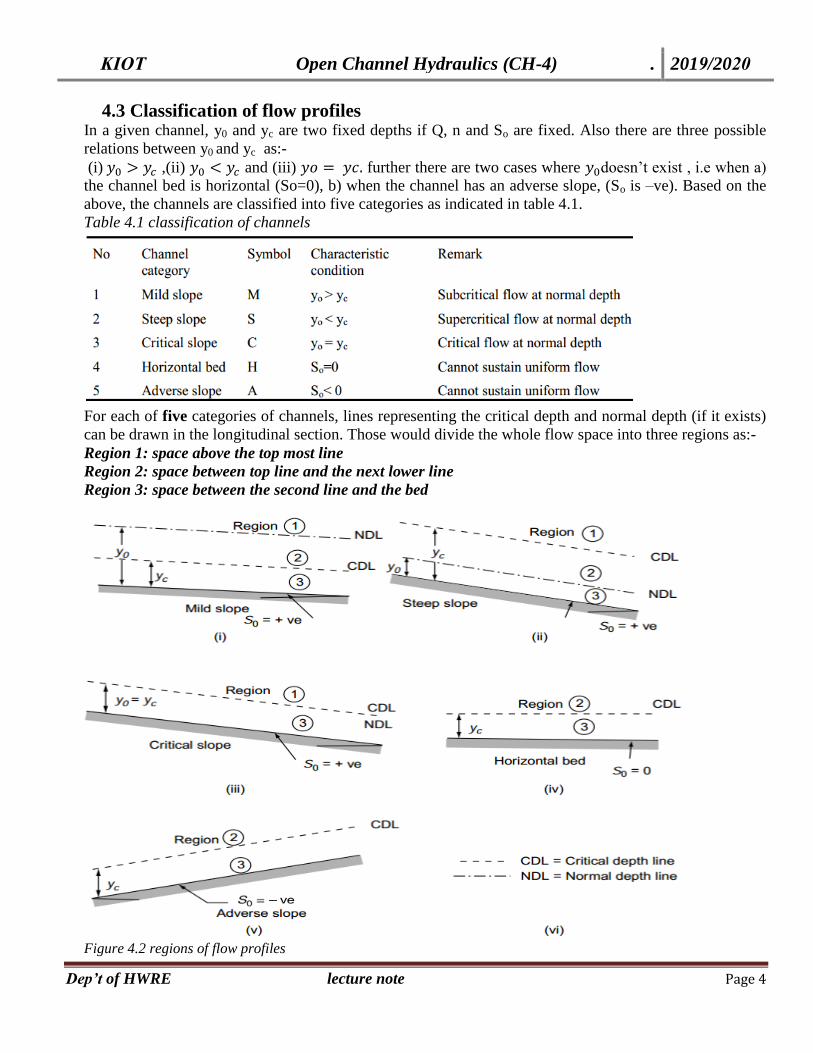
4.3 Classification of flow profiles In a given channel, y0 and yc are two fixed depths if Q, n and So are fixed. Also there are three possible

relations between y0 and yc as:-

(i) ,(ii) and (iii) further there are two cases where doesn’t exist , i.e when a)

the channel bed is horizontal (So=0), b) when the channel has an adverse slope, (So is –ve). Based on the

above, the channels are classified into five categories as indicated in table 4.1.

Table 4.1 classification of channels

For each of five categories of channels, lines representing the critical depth and normal depth (if it exists)

can be drawn in the longitudinal section. Those would divide the whole flow space into three regions as:-

Region 1: space above the top most line

Region 2: space between top line and the next lower line

Region 3: space between the second line and the bed

Figure 4.2 regions of flow profiles



Depending upon the channel category and region of flow, the water-surface profiles will have either of the

following characteristic shapes.

1. Back water curves: if the depth of flow increases in the direction of flow.

2. Drawdown curves: if the depth of flow decreases in the direction flow.

The dynamic equation of GVF expresses the longitudinal surface slope of flow with respect to the channel

bottom is given by:-



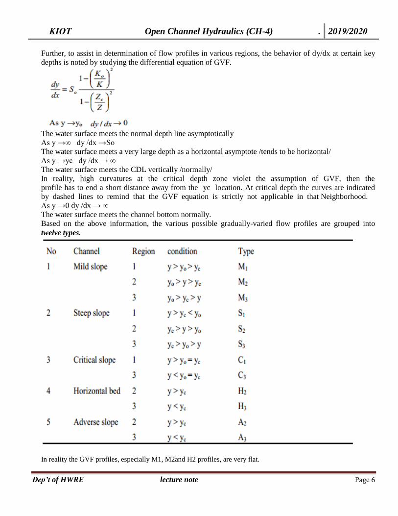
Further, to assist in determination of flow profiles in various regions, the behavior of dy/dx at certain key

depths is noted by studying the differential equation of GVF.

The water surface meets the normal depth line asymptotically

As y →∞ dy /dx →So

The water surface meets a very large depth as a horizontal asymptote /tends to be horizontal/

As y →yc dy /dx → ∞

The water surface meets the CDL vertically /normally/

In reality, high curvatures at the critical depth zone violet the assumption of GVF, then the

profile has to end a short distance away from the yc location. At critical depth the curves are indicated

by dashed lines to remind that the GVF equation is strictly not applicable in that Neighborhood.

As y →0 dy /dx → ∞

The water surface meets the channel bottom normally.

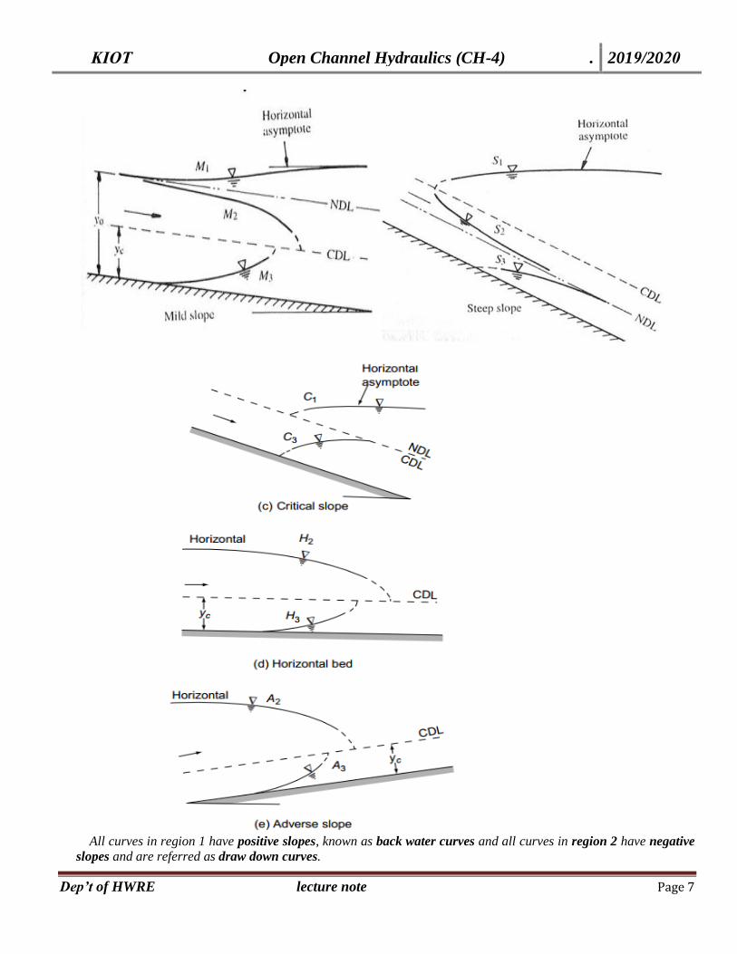
Based on the above information, the various possible gradually-varied flow profiles are grouped into

twelve types.

In reality the GVF profiles, especially M1, M2and H2 profiles, are very flat.



All curves in region 1 have positive slopes, known as back water curves and all curves in region 2 have negative

slopes and are referred as draw down curves.



4.4 same features of flow profiles

A). Type M flow profiles

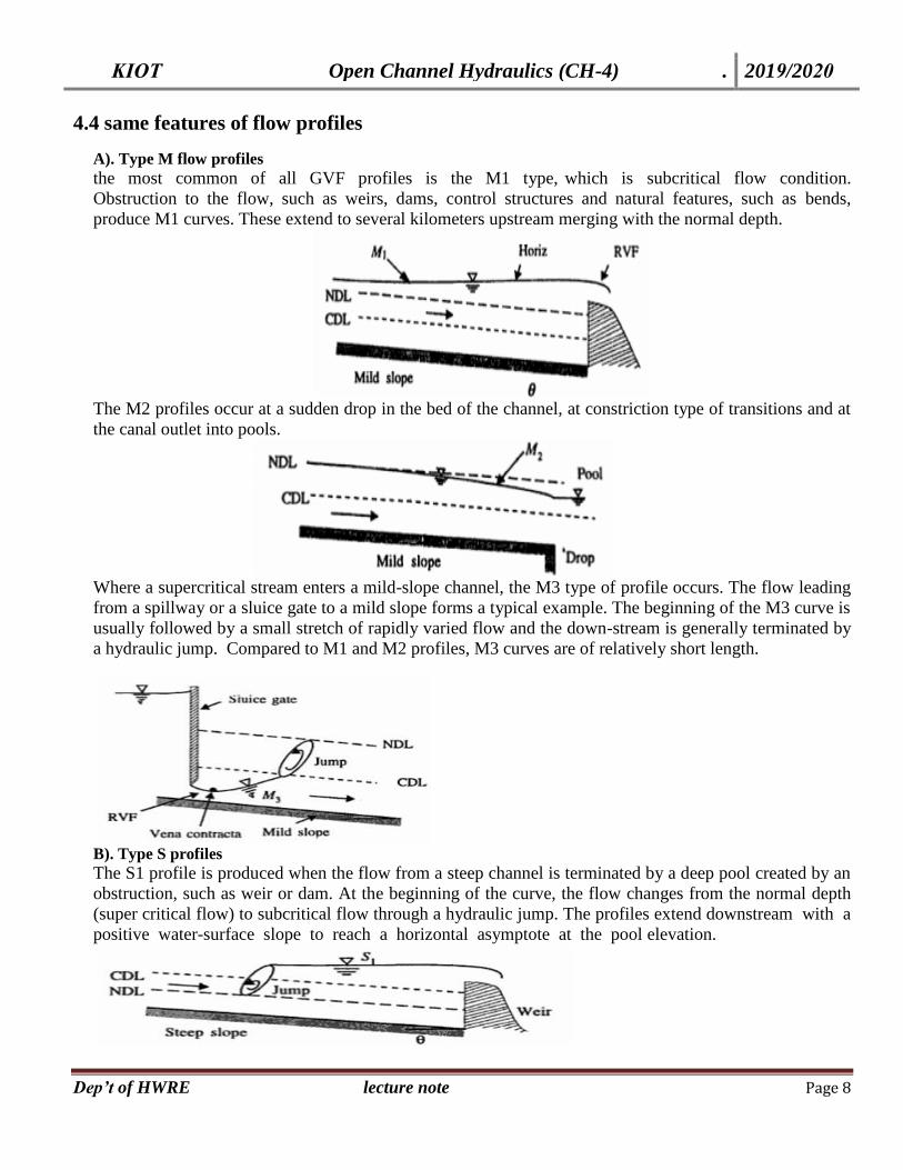
the most common of all GVF profiles is the M1 type, which is subcritical flow condition.

Obstruction to the flow, such as weirs, dams, control structures and natural features, such as bends,

produce M1 curves. These extend to several kilometers upstream merging with the normal depth.

The M2 profiles occur at a sudden drop in the bed of the channel, at constriction type of transitions and at

the canal outlet into pools.

Where a supercritical stream enters a mild-slope channel, the M3 type of profile occurs. The flow leading

from a spillway or a sluice gate to a mild slope forms a typical example. The beginning of the M3 curve is

usually followed by a small stretch of rapidly varied flow and the down-stream is generally terminated by

a hydraulic jump. Compared to M1 and M2 profiles, M3 curves are of relatively short length.

B). Type S profiles

The S1 profile is produced when the flow from a steep channel is terminated by a deep pool created by an

obstruction, such as weir or dam. At the beginning of the curve, the flow changes from the normal depth

(super critical flow) to subcritical flow through a hydraulic jump. The profiles extend downstream with a

positive water-surface slope to reach a horizontal asymptote at the pool elevation.

KIOT Open Channel Hydraulics (CH-4) . 20192020


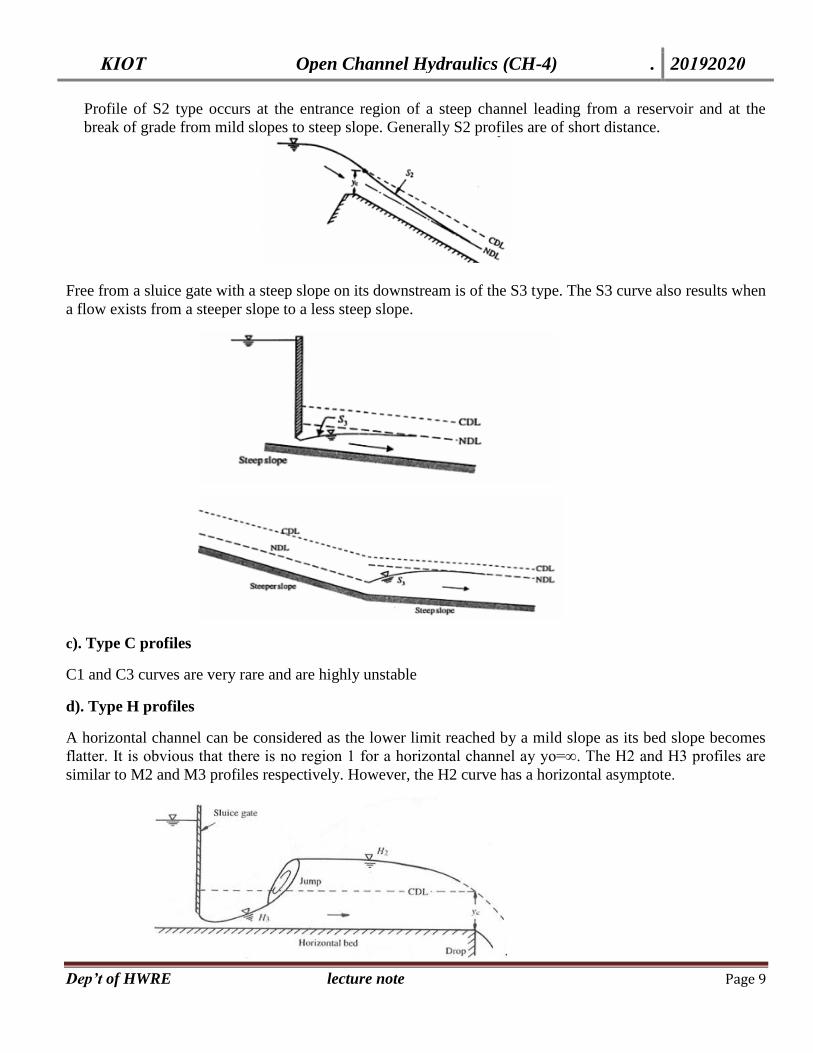
Profile of S2 type occurs at the entrance region of a steep channel leading from a reservoir and at the

break of grade from mild slopes to steep slope. Generally S2 profiles are of short distance.

Free from a sluice gate with a steep slope on its downstream is of the S3 type. The S3 curve also results when

a flow exists from a steeper slope to a less steep slope.

c). Type C profiles

C1 and C3 curves are very rare and are highly unstable

d). Type H profiles

A horizontal channel can be considered as the lower limit reached by a mild slope as its bed slope becomes

flatter. It is obvious that there is no region 1 for a horizontal channel ay yo=∞. The H2 and H3 profiles are

similar to M2 and M3 profiles respectively. However, the H2 curve has a horizontal asymptote.



e). type A profiles

Adverse slopes are rather rare and A2 and A3 curves are similar to H2 and H3 curves respectively. The

profiles are of very short length.

4.5. Control section

A control section is defined as a section in which a fixed relationship exists between the discharge and depth

of flow. Weirs, spillways, sluice gates are some typical examples of structures which give rise to control

sections. The critical depth is also a control point. However, it is effective in a flow profile which changes

from subcritical to supercritical flow in the reverse case of transition from supercritical flow to subcritical

flow; a hydraulic jump is usually formed by passing the critical depth as a control point. Any GVF

profile will have at least one control point. This control sections provide a key to the identification of proper

profile shapes. A few typical control sections are indicated in the figure below.

Subcritical flows have controls in the downstream end while supercritical flows are governed by control

section existing at the upstream end of the channel section.



Fig 4.3 examples of control in GVF

4.6. Analysis of flow profiles

The process of identification of possible profiles as a prelude to quantitative computation is known as

analysis of flow profiles. A channel carrying a GVF can in general contain different prismoidal channel

sections of varying hydraulic properties. There can be a number of control sections at a various locations. To

determine the resulting water-surface profile in a given case, one should be in a position to analyses the

effect of various channel sections and controls connected in series.

Break in grade (Serial Combination of Channel Sections)

Simple situation of a serious combination of two channel sections with differing bed slopes are

connected in the figure below. The grade changes acts as a control section and this can be classified as a

natural control. Various combinations of slopes and the resulting GVF profiles are presented in the figure

below. It may be noted that in some situation there can be more than one possible profile.

Procedure to draw the profile of GVF in grade transition:-

1. Draw the longitudinal section of the system.

2. Calculate the critical depth and normal depths of various reaches and draw the CDL and NDL in all

reaches. Since yc doesn’t depend upon the slope CDL will be constant above the channel bed in both

slopes.

3. Mark all the controls, both the imposed as well as natural controls.

4. Identify the possible profiles.

5. The normal depth for the mild slope is lower than that of the milder slope in this case the second depth acts as a

control.



Various combinations of slopes and the resulting GVF profiles are presented in the figure below. It may be

noted that in some situation there can be more than one possible profile.

Figure 4.4 GVF profiles at breaking grade



4.7 GVF Computations

Almost all major hydraulic engineering activities in the free surface flow involve the computation of

GVF profiles. Gradually varied Involves the solution of the dynamic equation.the main objective is to

determine the shape of flow profile.the flow computation is needed to analyze problems such as

Determination of effect of a hydraulic structure on the channel

Inundation due to a dam or weir construction

Estimation of flood zone

Broadly classified there are three Methods of GVF computations

1. Numerical method

2. Direct integration

3. Graphical method

Out of these the graphical method is practically obsolete and is seldom used. Further the numerical method is

the most extensively used technique. In the form of a host of available compressive

Software’s it is the only method available to solve practical problem in natural channels. The direct

integration technique is essentially of academic interest.

4.7.1 Numerical method The numerical solution procedure to solve GVF problems can be broadly classified into two categories as:

a. Simple numerical methods

These were developed primarily for hand computation. they usually attempt to solve the energy equation

either in the form of the differential energy equation of GVF or in the form of the Bernoulli equation.

b. Advanced Numerical Methods

These are normally suitable for use in digital computers as they involve a large number of repeated

calculations. They attempt to solve the differential equation of GVF.

Two commonly used simple numerical methods to solve GVF problems are :

1. Direct-step method

2. Standard-step method

4.7.1.1 The Direct Step Method (Distance from Depth)

The direct step method is a simple method applicable to prismatic channels. Depths of flow are specified and

the distances between successive depths are calculated. The equation may be used to determine directly (with

means explicit) the distance between given differences of depth y.

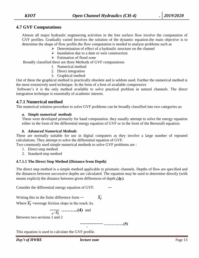
Consider the differential energy equation of GVF.

Writing this in the finite difference form

Where =average friction slope in the reach Δx.

………..(4) and

Between two sections 1 and 2

……………(5)

This equation is used to calculate the GVF profile.



The hydraulic elements are independent of the distance along the (prismatic) channel. An approximate

analysis can be achieved by dividing the channel in a number of successive, short reaches. For each of the

reaches the water depth at the beginning can be estimated.

Next the length of reaches can be calculated (step by step) from one end of the reach to the other end. The

Chezy or Manning formula is applied to average conditions in each reach to provide an estimate of and

So, with the depth and velocity at one end of the reach given, the length can be computed. Depths of flow are

specified and the distances between successive depths are calculated.

Figure 4.5 the Channel Reach for derivation of direct step method

Procedure

Referring to figure 4.5 , let it be required to find the water surface profile between two section 1 and (N+1)

where the depth are y1 and yN+1 respectively. The channel reach is now divided into N part of known depths,

i.e values of yi i=1,N are known .it is required to find the distance Δxi between yi and yi+1.Now between the

two sections i and i+1.

The sequential evaluation of Δxi starting from i=1 to N, will give the distance between the N sections and

thus the GVF profile. The process is explicit and is best done in a tabular manner.

For the computations the following are needed:

Discharge Q

Depth of flow y

Area A

Hydraulic radius R

Roughness coefficient n or C

Coefficient of Coriolis α

1 2 3 4 5 6 7 8 9 10 11 12 13

SL.No y(m) A(m2) P(m) R(m) V( ⁄ E(m) ΔE(m) Sf Δx x



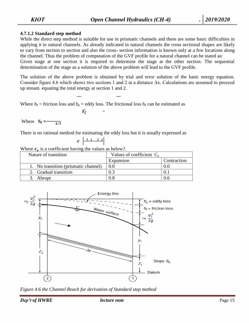
4.7.1.2 Standard step method

While the direct step method is suitable for use in prismatic channels and there are some basic difficulties in

applying it to natural channels. As already indicated in natural channels the cross sectional shapes are likely

to vary from section to section and also the cross- section information is known only at a few locations along

the channel. Thus the problem of computation of the GVF profile for a natural channel can be stated as:

Given stage at one section it is required to determine the stage at the other section. The sequential

determination of the stage as a solution of the above problem will lead to the GVF profile.

The solution of the above problem is obtained by trial and error solution of the basic energy equation.

Consider figure 4.6 which shows two sections 1 and 2 at a distance Δx. Calculations are assumed to proceed

up stream. equating the total energy at section 1 and 2.

Where hf = friction loss and he = eddy loss. The frictional loss hf can be estimated as

Where Sf = ⁄

There is no rational method for estimating the eddy loss but it is usually expressed as

| |

Where is a coefficient having the values as below?.

Nature of transition Values of coefficient Ce

Expansion Contraction

1. No transition (prismatic channel) 0.0 0.0

2. Gradual transition 0.3 0.1

3. Abrupt 0.8 0.6

Figure 4.6 the Channel Reach for derivation of Standard step method



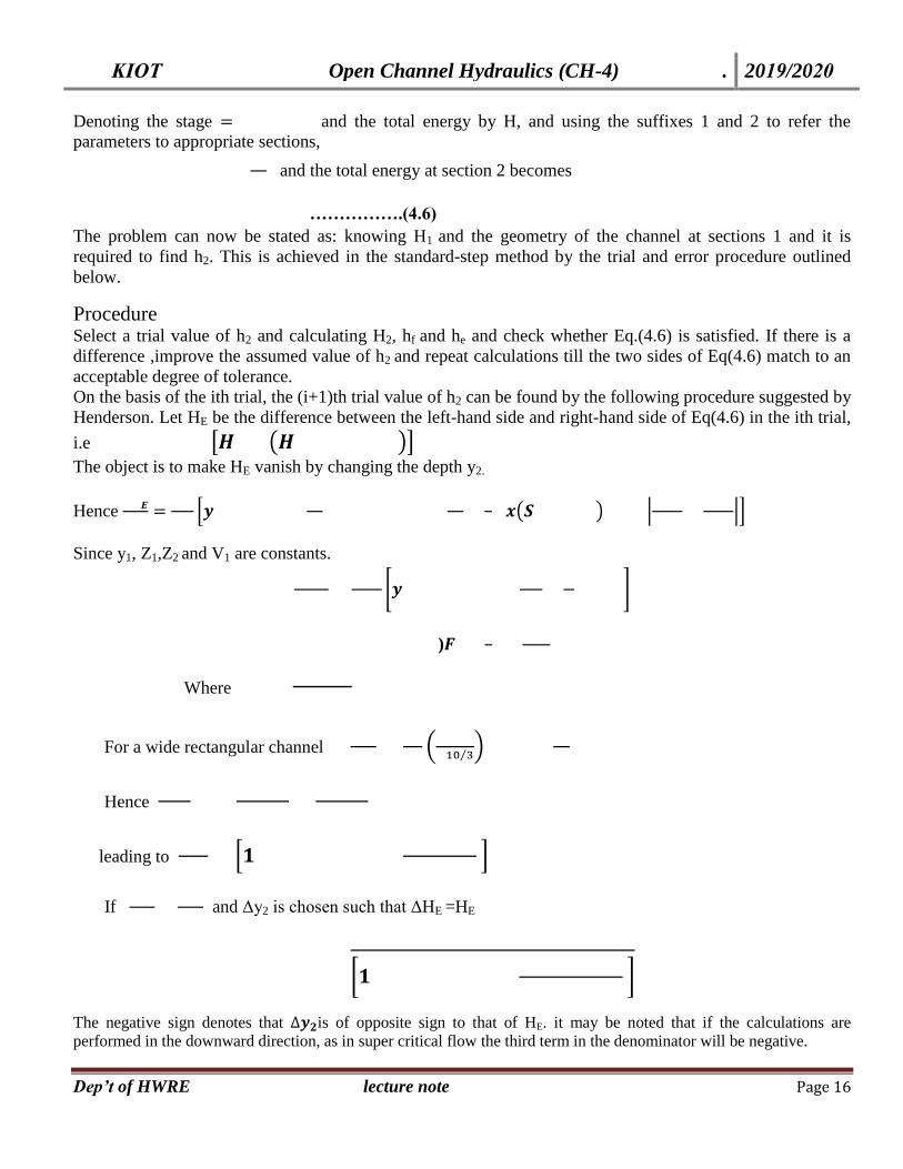
Denoting the stage and the total energy by H, and using the suffixes 1 and 2 to refer the

parameters to appropriate sections,

and the total energy at section 2 becomes

…………….(4.6)

The problem can now be stated as: knowing H1 and the geometry of the channel at sections 1 and it is

required to find h2. This is achieved in the standard-step method by the trial and error procedure outlined

below.

Procedure

Select a trial value of h2 and calculating H2, hf and he and check whether Eq.(4.6) is satisfied. If there is a

difference ,improve the assumed value of h2 and repeat calculations till the two sides of Eq(4.6) match to an

acceptable degree of tolerance.

On the basis of the ith trial, the (i+1)th trial value of h2 can be found by the following procedure suggested by

Henderson. Let HE be the difference between the left-hand side and right-hand side of Eq(4.6) in the ith trial,

i.e [ ( )]The object is to make HE vanish by changing the depth y2.

Hence * ( ) | |+

Since y1, Z1,Z2 and V1 are constants.

[ ]

)

Where

For a wide rectangular channel ( ⁄ )

Hence

leading to * +

If and Δy2 is chosen such that ΔHE =HE

[ ]

The negative sign denotes that is of opposite sign to that of HE. it may be noted that if the calculations are

performed in the downward direction, as in super critical flow the third term in the denominator will be negative.



For the computation the following data are needed: Discharge Q

Length of the reach Δx

Area A as function of y

Hydraulic radius R as function of y

Roughness coefficient ( n or C)

Carioles coefficient

The computation of the flow profile by the standard step method is arranged in tabular form

Stat

-ion

trial Elevatio

n of bed

z(m)

y

depth

(m)

h or Z

stage

(z+y)

(m)

A

(m2)

(m)

H

Total

head

(m)

R

(m)

Sf

Units

of

10-4

Units

of

10-4

Length

of

reach

(m)

hf

(m)

he

(m)

Total

head

(m)

HE

(m) (m)

1(a) 1(b) 2 3 4 5 6 7 8 9 10 11 12 13 14 15 16

Each column of the table is explained as follows:

1. The location of the stations is fixed.

2. Water-surface elevation Z at the station. A trial value is first entered in this column; this will be

verified or rejected on the basis of ht computations made in the remaining columns of the table.

For the first step, this elevation must be given or assumed. In most cases the first entry is known.

After this value in the second step has been verified, it becomes the basis for the verification the

trial value in the next step, and so on.

3. Depth of flow y corresponding to the water-surface elevation in col. 2. For instance, the depth of

flow y at the second station is equal to water-surface elevation minus bottom elevation (distance from

the first site times bed slope)

4. Water area A corresponding to y in col.3

5. Mean velocity v equal to the given discharge divided by the water area in col. 4

6. Velocity head in m, corresponding to the velocity col. 5

7. Total head E computed, equal to the sum of Z in col. 2 and the velocity head in col. 6

8. Hydraulic radius R corresponding to y in col. 3

9. Friction slope Sf with n or C, V from col. 5 and R from col. 8

10. Average friction slope through the reach between the sections in each step, approximately equal to

the arithmetic mean of the friction slope just computed in col. 9 and that of the previous step.

11. Length of the reach (∆x) between the sections.

12. Friction loss in the reach, equal to the product of the values in cols. 10 and11.

13. transition loss in the reach he (m)

14. Elevation of the total head E. this is computed by adding the values of hf (and he if calculated in a

previous column) in col. 14 to the elevation at the lower end of the reach, which is found in col. 14 of

the previous reach. If the value so obtained does not agree closely with that entered in col. 7, a new

trial value of the water-surface elevation is assumed, and so on, until agreement is obtained. The

value that leads to agreement is the correct water-surface elevation. The computation may then

proceed to the next step.



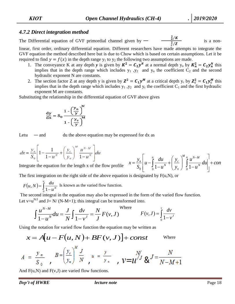
4.7.2 Direct integration method

The Differential equation of GVF primordial channel given by ⁄

⁄

is a non-

linear, first order, ordinary differential equation. Different researchers have made attempts to integrate the

GVF equation the method described here but is due to Chow which is based on certain assumptions. Let it be

required to find in the depth range y1 to y2 the following two assumptions are made. 1. The conveyance K at any depth y is given by

at a normal depth yn by

this

implies that in the depth range which includes y1 ,y2 and yn the coefficient C2 and the second

hydraulic exponent N are constants.

2. The section factor Z at any depth y is given by at a critical depth yc by

this

implies that in the depth range which includes y1 ,y2 and yc the coefficient C1 and the first hydraulic

exponent M are constants.

Substituting the relationship in the differential equation of GVF above gives

Let and du the above equation may be expressed for dx as

Integrate the equation for the length x of the flow profile

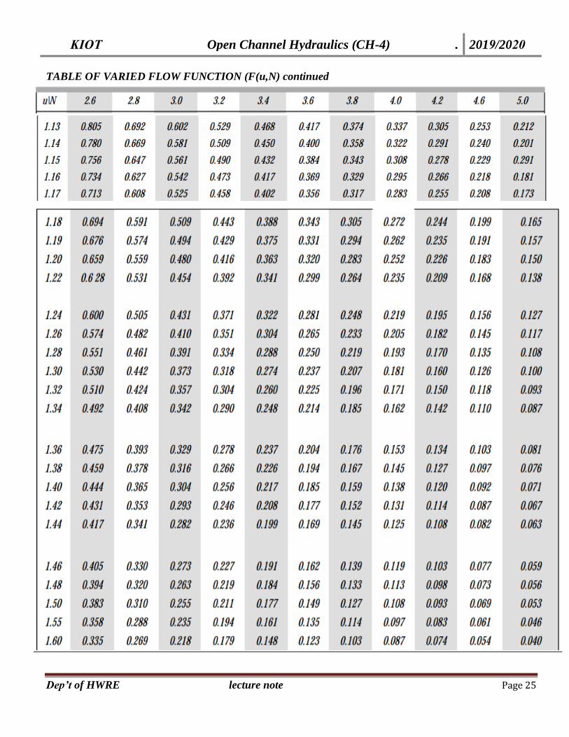
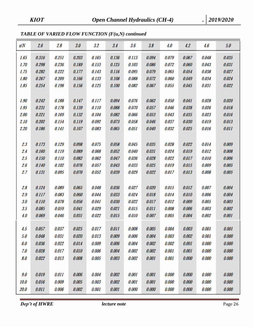
The first integration on the right side of the above equation is designated by F(u,N), or

Is known as the varied flow function.

The second integral in the equation may also be expressed in the form of the varied flow function.

Let v=uN/J

and J= N/ (N-M+1); this integral can be transformed into.

– Where

Using the notation for varied flow function the equation may be written as

Where

And F(u,N) and F(v,J) are varied flow functions.

conduu

u

y

y

u

duu

S

yx

u u

N

MNM

n

c

N

n

0 00 11

u

Nu

duNuF

01

,

),(11

JvFJ

N

v

dv

N

Jdu

u

uJN

MN

v

Jv

dvJvF

01

),(

constJvBFNuFuAx ),(,



The length of flow profile between two consecutive section 1 and 2 is equal to L = x2-x1

Where the subscripts 1 and 2 refers to sections 1 and 2, respectively.

The computation of the flow profile by the direct integration method is arranged in tabular form

1 2 3 4 5 6 7 8 9

S.No. y(m) u v F(u,N) F(v,J) x(m) Δx(m) L(m)

1.

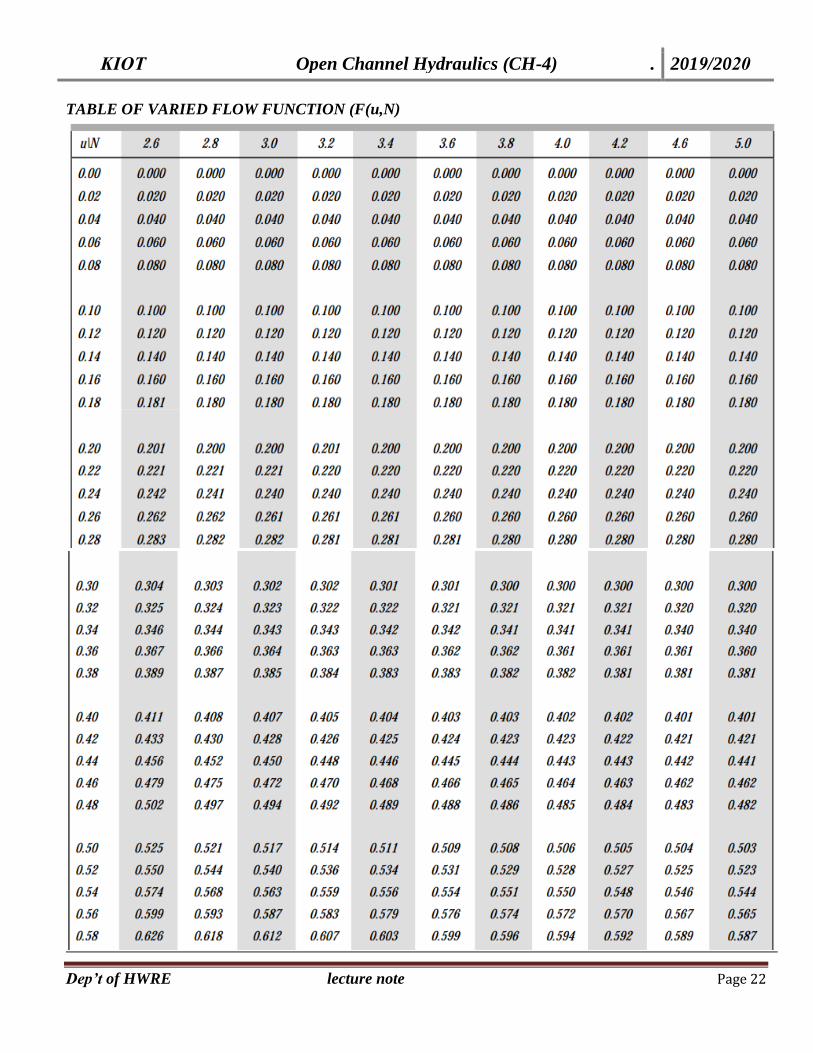
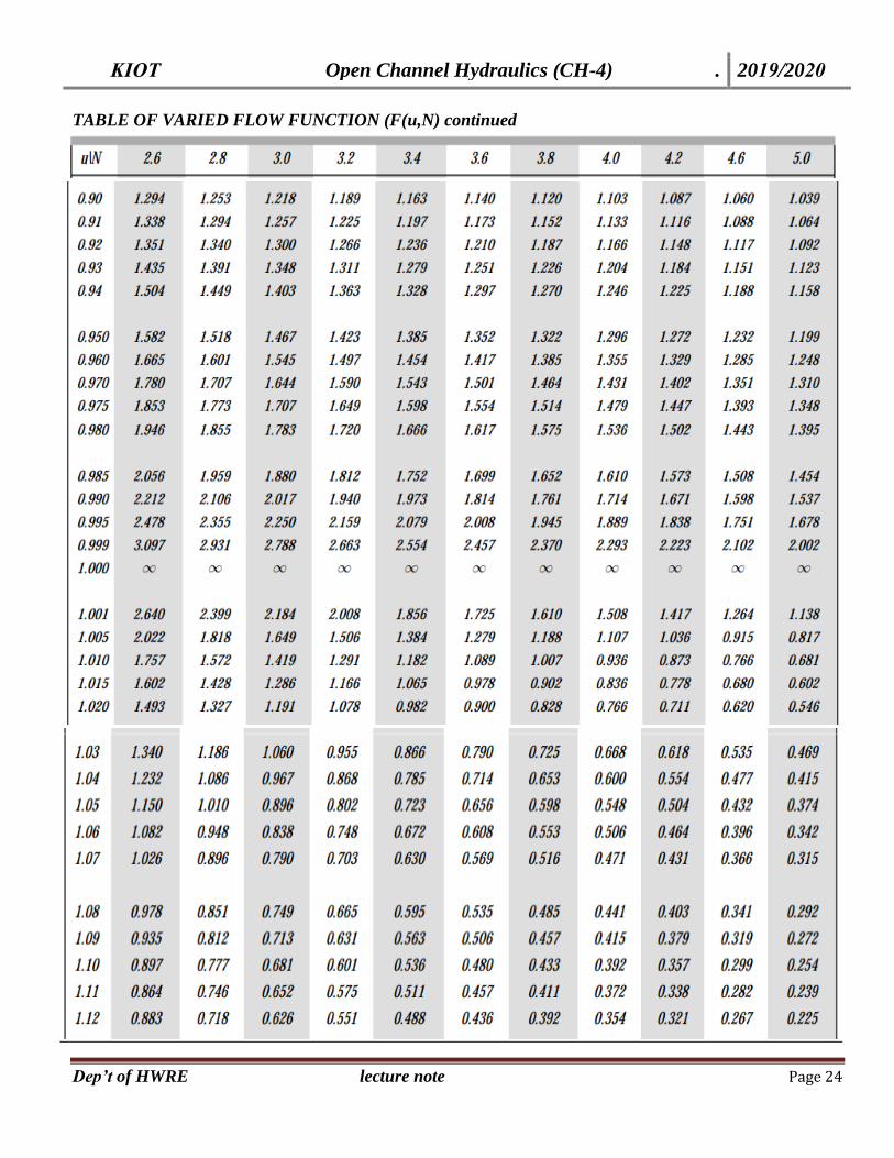
For varied flow function make use of the varied-flow-function table given in tables (at the end of this

chapter, appendix D of Ven Te Chow or at the end of chapter 5 of Subramaniya)

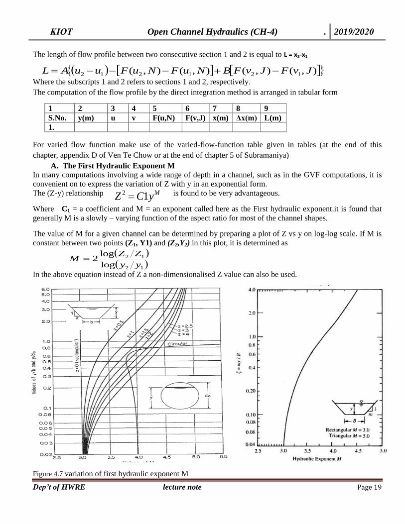
A. The First Hydraulic Exponent M

In many computations involving a wide range of depth in a channel, such as in the GVF computations, it is

convenient on to express the variation of Z with y in an exponential form.

The (Z-y) relationship is found to be very advantageous.

Where C1 = a coefficient and M = an exponent called here as the First hydraulic exponent.it is found that

generally M is a slowly – varying function of the aspect ratio for most of the channel shapes.

The value of M for a given channel can be determined by preparing a plot of Z vs y on log-log scale. If M is

constant between two points (Z1, Y1) and (Z2,Y2) in this plot, it is determined as

In the above equation instead of Z a non-dimensionalised Z value can also be used.

Figure 4.7 variation of first hydraulic exponent M

),(),(),(),( 121212 JvFJvFBNuFNuFuuAL

MyCZ 12

12

12

log

log2

yy

ZZM



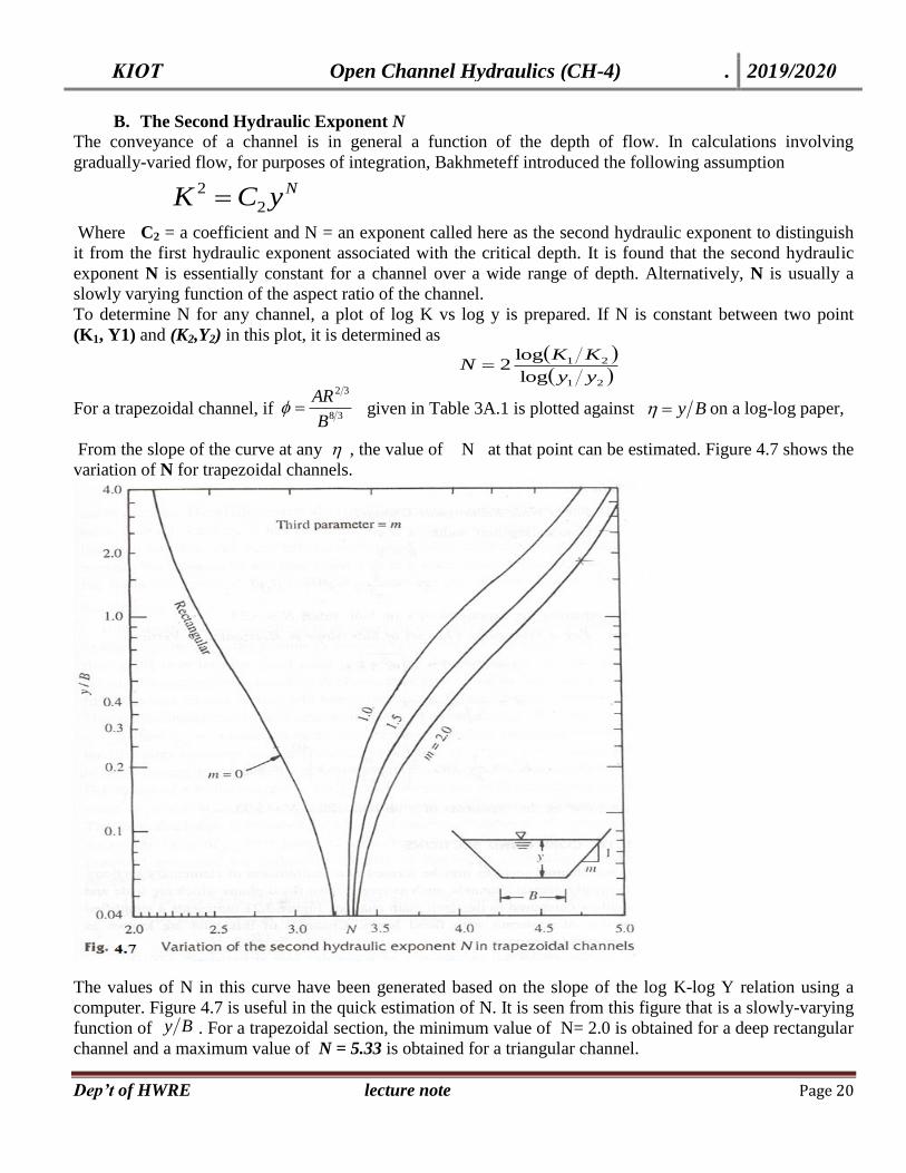
B. The Second Hydraulic Exponent N

The conveyance of a channel is in general a function of the depth of flow. In calculations involving

gradually-varied flow, for purposes of integration, Bakhmeteff introduced the following assumption

Where C2 = a coefficient and N = an exponent called here as the second hydraulic exponent to distinguish

it from the first hydraulic exponent associated with the critical depth. It is found that the second hydraulic

exponent N is essentially constant for a channel over a wide range of depth. Alternatively, N is usually a

slowly varying function of the aspect ratio of the channel.

To determine N for any channel, a plot of log K vs log y is prepared. If N is constant between two point

(K1, Y1) and (K2,Y2) in this plot, it is determined as

For a trapezoidal channel, if given in Table 3A.1 is plotted against on a log-log paper,

From the slope of the curve at any , the value of N at that point can be estimated. Figure 4.7 shows the

variation of N for trapezoidal channels.

The values of N in this curve have been generated based on the slope of the log K-log Y relation using a

computer. Figure 4.7 is useful in the quick estimation of N. It is seen from this figure that is a slowly-varying

function of . For a trapezoidal section, the minimum value of N= 2.0 is obtained for a deep rectangular

channel and a maximum value of N = 5.33 is obtained for a triangular channel.

NyCK 2

2

21

21

log

log2

yy

KKN

38

32

B

AR By

By



4.7.3 Graphical Integration Method

Consider two channel sections at distance x1and x2 and with corresponding depths of flow y1and y2. The

distance along the channel is x. If a graph of y against f(y) is plotted, then the area under the curve is

equivalent to x. The value of the function f(y) may be found by substitution of A, P, So and Sf for various

values of y and for a given Q. Hence, the distance X between the given depths (y1and y2) may be calculated

(numerical integration) or measured (graphical integration).this numerical/graphical method gives the

distance from depth.

This method integrates the equation of gradually varied flow by a numerical procedure.

Figure 4.9 The Channel Reach for derivation of Graphical Integration

By this method the largest errors are found in the area with the strongest curvature. This is the region near the

control point(s). The accuracy can be improved by varying the steps x as a function of the curvature. This

method has broad application. It applies to flow in prismatic as well as non-prismatic channels of any shape

and slope. The procedure is straightforward and easy to follow. It may become very laborious when applied

to actual field problems.



TABLE OF VARIED FLOW FUNCTION (F(u,N)



TABLE OF VARIED FLOW FUNCTION (F(u,N) (continued)



TABLE OF VARIED FLOW FUNCTION (F(u,N) continued

chapter four gradually varied flow (gvf) 4.1 general

Documents