chapter iv. 1-d particle motion
TRANSCRIPT

4-1
Chapter IV. 1-D Particle Motion
4.1. Introduction 1-D particle motion is a good place to gain a fundamental understanding of mechanics – we'll build upon this information in subsequent chapters. This is the fun part because it lays the foundation for solving interesting meteorological problems. For simplicity, we assume that the motion is along the x axis only. The goal is to predict the motion of a system when the interactions (forces) are known (it gets more complicated when you also have to predict the forces and the forces depend on the flow – nonlinearity).
4.2. Work-Energy Theorem The starting point is Newton's 2nd Law:
dv d dxm m F
dt dt dt = =
(1)
where v = dx/dt = speed along x-axis m = mass of particle F = net force acting on the particle. THIS EQUATION IS THE FOUNDATION FOR STUDYING ATMOSPHEREIC DYNAMICS – IT IS A SIMPLIFED FORM OF THE EQUATIONS OF MOTION THAT YOU'WLL STUDY IN DYNAMICS I (METR3113). SO LEARN THIS MATHERIAL WELL!! As an enticement, I will write down the equation that governs airflow in a thunderstorm updraft:
1dw p
gdt zρ
∂= − −
∂ (2)
Vertical Acceleration Pressure gradient force Gravitational Force (buoyancy) Here, w = updraft speed, ρ = air density, p = pressure, and g = gravity. The RHS is the force F, which is the sum of 2: PGF + weight of the air. Note that m does not appear explicitly – we look at things per unit mass, so that mass gets divided out. If you multiple Eq.(2) by ρ on both sides, we have
4-2
dw p
gdt x
ρ ρ∂
= − −∂
(3)
Eq.(3) looks more like (1) and now we are talking about an air parcel with unit volume.
Now go back to our problem 2
2
d xm F
dt= . One complication is that F can be a function of time and
space. This can be very serious, and is one major reason why we use computers – exact solutions are often not possible or known. To obtain physically meaningful solutions, we appeal to 2 useful concepts: WORK and ENERGY. Before getting to work and energy, we first introduce the concept of MOMENTUM defined as: P mv≡ . (4) It's mass times velocity. Using (4) in (1) gives
dP
Fdt
= (5)
which makes it clean that momentum can change by virtue of either velocity or mass (or both). Often this is called the differential momentum theorem. To get change in the momentum in a period of time, we integrating (5) from time t1 to t2:
2 2 2 2
1 1 1 1
( )
( )
t P t P t
t P t P t
dPdt dP Fdt
dt
=
=
= = ∫ ∫ ∫
2
12 1 Impulse
t
tP P Fdt∴ − = ≡∫ (6)
The impulse is the integrated force delivered over some period of time. Clearly, F(t) must be known to solve (6). In the atmosphere, we need to know P(x,t). (6) is the mementum theorem, which says
Impulse from the net force = change in momentum

4-3
Going back to (1) and multiplying both sides by v, we have (assuming that mass is constant):
dvvm Fv
dt=
or 2
2d v
m Fvdt
=
.
Assuming m = constant, we can write
2
2d v dK
m Fvdt dt
= ≡
(7)
where 2
2v
K m≡ is defined as Kinetic energy.
Integrating (7) gives
2
12 1 ( ) WORK
t
tK K Fv dt− = ≡∫ (8)
This RHS integral is known as the WORK done by the (net) force during the time interval t2 – t1. Suppose now that F is a known function of x. Then
dx dx
Fv F Fvdt F dt Fdxdt dt
= → = = ,
(8) becomes:
2
12 1
x
xK K Fdx− = ∫ (9)
This is the more familiar form and suggests that the work done by net force is related to the change of Kinetic Energy. This is the WORK-ENERGY THEOREM: Work done by net force = change in kinetic energy Note that the net force acting on an object changes the kinetic energy only, not potential energy (will be discussed later). E.g., when a crane lifts an object vertically at a uniform speed, it does work and changes the potential energy of the object. But since this lifting force equals the gravity, the net force acting on the object is zero, therefore there is no change in the kinetic energy.

4-4
SAMPLE PROBLEM: Suppose a mass m is thrown vertically upward with an initial speed vi. How high will it rise? Neglect friction and assume that g = constant. Apply your problem-solving techniques Typically the vertical coordinate is z: take it positive upward. Newton's 2nd law says F = - mg (no vector) Form (9), we have
2 2
( )2 2
f
i
zf if iz
mv mvFdz mg z z− = = − −∫ (10)
Solving (10) for zf à
2
2i
fv
zg
= .
Note – the solution is independent of the mass of the object (why?) and makes no reference to time. FOR YOU: Derive an expression for the time required to reach the peak of the trajectory. Be prepared to discuss your answer in class during the next lecture period. How is this problem important to meteorology? What important force has this problem neglected. The rotation of the earth! If you throw a ball upward, or if an air parcel moves upward, the earth rotates beneath it – when it comes back down, it won't land at the same spot where it was thrown! We will learn how big this effect is and find out how to take it into account later.
4.3. Problems with Flow-dependent Force Consider now the situation where the applied force is a function only of the velocity. From (1), we have (mass = constant)

4-5
( )dv
m F vdt
= . (11)
How can we solve this equation for the general case? What would you do first? Let's collect "like" terms:
1 1( )
dvF v dt m
= . (12)
Now we can, in principle, integrate:
0 0( )
v t
v t
dv dtF v m
=∫ ∫
In 1-D motion, the only force that depends on velocity is friction (also Coriolis force but not truly 1-D). Typically friction is larger when velocity increases. Imagine you drag a box across the floor, the friction is larger then you run than when you walk. The simplest representation of friction is the power law: F = (-1)n b vn (b – frictional coefficient). In all cases, the friction should be in opposite direction to the velocity, i.e., it always represents decelerational effect. EXAMPLE: An air parcel rises at an initial velocity w0, and it becomes neutrally buoyant at t = t0 and height z = z0 . Let Ffriction = - b w (b>0 and constant). Then, the equation of motion (Newton's 2nd law) is
dwm bw
dt= − (13)
Collecting w on the LHS and others on the RHS, as we did in (12), gives
dw bdt
w m= − (14)
Integrating (14), i.e.,
0 0
ln( )w t
w t
bd w dt
m= −∫ ∫ (15)

4-6
0 0ln( ) ln( ) ( )b
w w t tm
− = − −
00
ln ( )w b
t tw m
= − −
0 0exp ( )b
w w t tm
= − −
(16)
(16) is the final solution, for w at any time t. MAKE SURE YOU CAN DERIVE THIS RESULT WITHOUT REFERENCE TO THE NOTE!!! IF YOU DO NOT KNOW HOW WE GOT FROM (14) TO (16), GO BACK AND CHECK OUT YOUR CALCULUS BOOKS!!! It 's always good to examine the solution. First, does it satisfy the initial condition? Yes! w(t=0) = w0.
Does w increase or decrease with time? Since 0exp ( )b
t tm
− −
< 1 for 0t t− >0, w < w0, therefore
the parcel decelerates!! This is expected because the net force acting on the parcel was frictional force. Its weight was balanced by the upward pressure gradient force so that it was 'neutrally buoyant'. Next, are dimensions consistent? Yes. How about the exponential? The argument must be non-dimensional:
1
0( )
( ) ~ 1b kg s s
t tm kg
−
− − = - non-dimensional – correct!
Now, look at the asymptotic behavior! As , 0t w→ ∞ → . But note that, as long as t is finite, the parcel never comes to a stop. This is because the frictional force decreases as w decreases. As w approaches zero, the force approaches zero too. Makes sense! Finally, realize that the frictional effect is exponential with time – this is rather typical of damping / frictional effects. The rate of damping is proportional to b and inversely proportional to m. So, large m means less frictional effect!! If you throw a dart and a piece of feather at the same speed, which one is stopped more quickly by friction?

4-7
In addition to the damping rate, another often used measure of strength of friction or damping is the e-folding time of damping. It is the time needed to reduce a value to 1/e times of its initial value. It's clear that for the above case, the e- folding time is
mb
τ = . (17)
So the larger the frictional / damping coefficient b is, the shorter is the time needed to reduced w by a factor of 1/e. What if we want to know the position of the parcel at a given time? We only need to integrate w with respect to time, because w = dz/dt.
0 00 0exp ( )
z t
z t
bdz w t t dt
m = − − ∫ ∫ (18)
we find
[ ]00 01 exp[ ( ) / ]
w bz z b t t m
m= + − − − . (19)
Check the behavior of the solution as we did for the other one. Again make sure you know how to obtain (19) from (18)!
4.4. Non-linearity and Approximation via Taylor Series Expansion At this point, we will introduce a very useful tool for approximating functions known as (Taylor) series approximation. Taylor series expansion First, let's review the Taylor series expansion we learnt in Calculus. Given a function F(x) possessing derivatives of all orders, one can write a Taylor series expansion for F about the point x0 in the following ways: Form #1:
0 0
22
0 0 02
1( ) ( ) ( ) ( ) High-orderterms
2!x x
F FF x F x x x x x
x x∂ ∂
= + − + − +∂ ∂
(20)
Form #2 (most commonly used in fluid mechanics and meteorology)

4-8
Here, we simply replace x by x0+∆x in the above, where ∆x is a small increment about the point x0 :
0 0 0
2 2 3 3
0 0 2 3
( ) ( )( ) ( ) High-orderterms
2! 3!x x x
F F x F xF x x F x x
x x x∂ ∂ ∆ ∂ ∆
+ ∆ = + ∆ + + +∂ ∂ ∂
(21)
Points to note: 1). One can write a Taylor series as a function of 2 variables in the following manner:
0 0
2
0 0 0 0
1( , ) ( , ) High-orderterms
2!x x
F x x y y F x y x y F x y Fx y x y
∂ ∂ ∂ ∂+ ∆ + ∆ = + ∆ + ∆ + ∆ + ∆ + ∂ ∂ ∂ ∂
(22) Note that the ( ) terms raised to a power are actually operators and therefore involve mixed derivatives. For examples, we can expand the operator in the last term as
2 2 2 22 2
2 2( ) 2 ( )x y x x y yx y x x y y
∂ ∂ ∂ ∂ ∂∆ + ∆ = ∆ + ∆ ∆ + ∆ ∂ ∂ ∂ ∂ ∂ ∂
.
2). One can use positive and negative increments in Form #2, with the sign attached to the increments itself, i.e., +∆x and -∆x. This allows us to write two series in one:
0 0 0
2 2 3 3
0 0 2 3
( ) ( )( ) ( ) High-orderterms
2! 3!x x x
F F x F xF x x F x x
x x x∂ ∂ ∆ ∂ ∆
± ∆ = ± ∆ + ± +∂ ∂ ∂
By substituting or adding the series, we can arrive at various approximations for derivatives. For example, subtracting and solving for /F x∂ ∂ gives
0
0 0( ) ( )High-orderTerms
2x
F x x F x xFx x
+ ∆ − − ∆∂= +
∂ ∆. (23)
The first term on the right hand side is actually commonly used in numerical weather prediction as well as other computational fluid dynamics models as a finite difference approximation to a partial derivative. Applying the above Taylor series formula, we can find the series expansion for most common functions. Those of most basic functions can be found in mathematics handbooks. For example,

4-9
2 3
1
1 ... 12! 3! !
nx
n
x x xe x x
n
∞
=
= + + + + = + − ∞ < < ∞∑ (24)
sin(x) = 3 5 7
...3! 5! 7!x x x
x x− + − + − ∞ < < ∞
cos(x)= 2 4 6
1 ...2! 4! 6!x x x
x− + − + − ∞ < < ∞
(25)
(you can tell from the above two which one is even and which is odd function of x)
Usually these series converges to the original function when n (the number of terms) approaches ∞ , but many do so only for values of x in a limited range. Approximating Solutions with Taylor Series Expansion Now, let go back to solution (16), the solution for w we found in last subsection
0 0exp ( )b
w w t tm
= − −
For relatively small values of 0( )b
t tm
− , i.e., when friction is weak and/or the time after t0 is short,
we can approximate the solution as
2 2
0 212
b t b tw w
m m ∆ ∆
≈ − +
, (26)
where the higher order terms are neglected. If we also neglect the second-order term, we have
0 1b t
w wm∆ ≈ −
(27)
Note that the first 2 terms in (26)?are what one would obtain for a constant force (-bw0, verify for yourself). Thus, the variable force (dependent on w) creates what we call a high-order effect.
2 20 0
0 22w b t w b t
w wm m
∆ ∆≈ − +
Zero order 1st order 2nd order

4-10
Further, this problem introduces us to the absolute key issue of physics and meteorology, and that is NONLINEARITY. Life would be very simple if systems behave in a linear way. However, they don’t. Let’s take a closer look before we examine conservative forces. Nonlinearity There are many different ways to describe this property – from qualitative / descriptive to very mathematical and precise. We will start with the former. A nonlinear system is typically characterized by a single important property – feedback! Let’s look at some common examples. CASE I: Heroine or any addictive substance. It is nonlinear in 2 ways. First, the more you use, the more you "need" it. This is a feedback. If it were linear, there would be no change in your "need". Second, your body tends to get used to it, so eventually you need something stronger. CASE II: Eating. The more you eat, the bigger you get, the bigger you get, the more you need to get fed à you get even bigger. CASE III: The lift on an airplane wing goes as the squared of the speed over the wings. Nonlinearity in this case is very helpful!
Air speed Linear lift Nonlinear lift
50 50 2,500 100 100 10,000 150 150 22,500 200 200 40,000
∆speed = constant ∆lift increases with speed Lift Air speed
Linear
Nonlinear - quadratic

4-11
Now, let's turn to the mathematical definition or explanation. This can get quite rigorous, and we'll deal with some of that later on. But for the time being, we will characterize a problem as linear (typically a differential equation) if: a) The dependent variable is raised to some power, i.e., multiplied by itself, or b) The derivative of a dependent variable is raised to certain power. Example:
2
5dx
xdt
+ = or 2 5dx
x xdt
+ = is a nonlinear ODE (Ordinary differential equation)
5du
u xdt
+ = or 2
52
d ux
dt
+ =
is a nonlinear ODE
Quite often in mechanics, we will convert a nonlinear equation into a linear equation because the latter often have exact solutions. One can view the solution so-obtained as the low-order term in a series of expansion, e.g.,
2 3
1 ...2! 3!
x x xe x≈ + + + +
1xe ≈ : zero-order term
1xe x≈ + : first order or linear term
2
12!
x xe x≈ + + : this the first nonlinear (here quadratic) term
If x is small, 1xe x≈ + is a pretty good approximation. Why? Let's check the accuracy:
e5 = 148.4131591 Zero-order e5 = 1 First-order e5 = 1 + 5 = 6 Second-order e5 = 1 + 5 + 52/2! = 18.5

4-12
Note that "x" is not small, and thus one needs quite a few terms. Check for yourself the case of e0.2. Do you think it will take fewer terms?
4.5. Total Energy Conservation and Stability Total Energy Conservation For the next 2 years, and certainly if you go to grad school, you will hear a lot about conservation, conservation laws, and conservative quantities. This will be our first look at them. Later, we will see that conservative forces lead to work that is independent of path. Consider the special case where F = F(x) only. Then,
( )dv
m F xdt
= (28)
and by (9) ( 2
12 1
x
xK K Fdx− = ∫ ), we have
0
2 20
1 1( )
2 2
x
xmv mv F x dx− = ∫ (29)
We now define the POTENTIAL ENERGY [V(x)] as the work done by the force when the particle goes from an arbitrary point x to some standard point xs (e.g., the sea level):
( ) ( ) ( )s
s
x x
x xV x F x dx F x dx≡ = −∫ ∫ (30)
The above is the mathematical definition of potential energy. Why do we call it potential energy? We will see this later. But for now, note that, in meteorology, there are many examples of "potential" quantities: - potential energy (e.g., convective available potential energy CAPE) - potential vorticity Perhaps the most common is potential temperature – it is the temperature that an air parcel has if it is moved from its present location to 1000mb via an adiabatic process, i.e., there is no exchange of heat with its surrounding. Note that, in this case, 1000mb is the reference point – the same as xs above. It could be anything, but 1000mb is the agreed upon standard. Potential temperature is conserved for dry adiabatic motion.
4-13
Now, return to our example. Going back to (29), we see that we can write the following:
0 0
2 20
0
1 1( ) ( ) ( )
2 2( ) ( )
s
s
x x x
x x xmv mv F x dx F x dx F x dx
V x V x
− = = +∫ ∫ ∫
thus
2 20 0
1 1( ) ( )
2 2mv V x V x mv+ = +
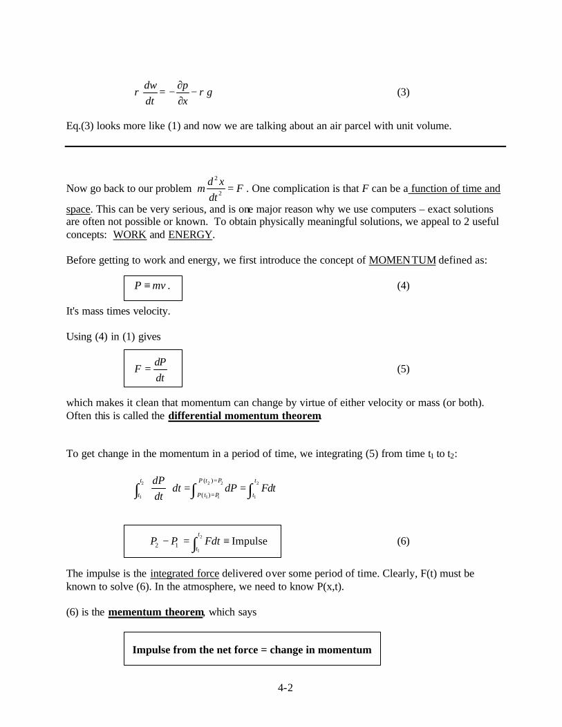
only a function of I.C. and is thus constant during the motion. We define the RHS as the TOTAL (mechanical) ENERGY ≡ E, Now we have a Conservation Law: E = KE + PE = constant following the motion (31) Or ∆E = 0. Important Note! This is true only when the applied force is a function of position only, i.e., F=F(x) and not F(v) or F(t). Such a force is called conservative force. More on this later. Going back to the integral that defines the PE (V), we see that
F = - dV/dx (32) This is the physical statement of the PE and is how you should learn it – the negative gradient of the PE gives the force. If you recall your study of electric fields, you will note that the gradient of the electric potential is equal to the electrostatic force. E = - dV/dx F

4-14
5 10 15 20 Note that, since the derivative of V is what matters, the choice of xs is arbitrary – one can always add a constant to V and not affect the force. Usefulness of Total Energy Conservation So what is the energy conservation law good for? Since we know the total energy is a conserved quantity, it does not change along its path of a 1-D particle motion. We can determine the total energy from the initial condition (i.e., at t=t0), and solve for one energy (e.g., kinetic energy) given the other (e.g., potential energy). Even without actually solving the equations, we can often gain physical insight into the behavior of mechanical or fluid dynamical systems. Look at the example shown in the following figure:
It shows the behavior of potential energy as a function of the x coordinate. We know the total energy, E, is conserved: KE + PE = Total energy = E.

4-15
From the curve of PE, we can get an idea of what kinds of motion that are possible for a particle whose initial position is x0. 1) If the total energy E = E0, the minimum possible PE, then there is no room for KE, i.e., KE has
to be zero, and the particle has to remain at rest. 2) If the particle's total energy E = E1, then particle can move between x1 and x2 – the turning
points. When it is at x0, PE is at a minimum therefore KE is at a maximum, i.e., the particle moves fastest at x0.
3) If E > E5, then the particle can move in either direction indefinitely, and never return. 4) For other values of E, discuss the behavior of the particle yourself. Applications in Meteorology and Stability Now, we will begin to apply these concepts to meteorology. First, let's introduce the concept of Stable Equilibrium, a state with minimum PE. Assume that V(x) is a minimum at x=x0. Now apply Taylor series expansion for V(x+x0):
0 0 0
2 32 3
0 0 2 3
1 1( ) ( ) ( ) ( ) ...
2! 3!x x x
dV d V d VV x x V x x x x
dx dx dx+ ∆ = + ∆ + ∆ + ∆ +
Since we know that V(x0) is a minimum, according to basic calculus, 0
0x
dVdx
= , and 2
2
d Vdx
> 0
(concave upward), therefore
0
22
0 0 2
1( ) ( ) ( )
2! x
d VV x x V x x
dx+ ∆ ≈ + ∆ , (33)
(for small values of ∆x, the high-order terms become small very fast, so they can be neglected safely without affecting the value of V much) therefore V at the neighborhood of x0 is always larger than V at x0 – makes sense because v(x0) is a minimum. DEFINITION : The point where V(x) has a minimum value is called a point of STABLE EQUILIBRIUM. This concept is one of the most important that you will ever use in the field of meteorology!! We will consider 3 different situations:
4-16
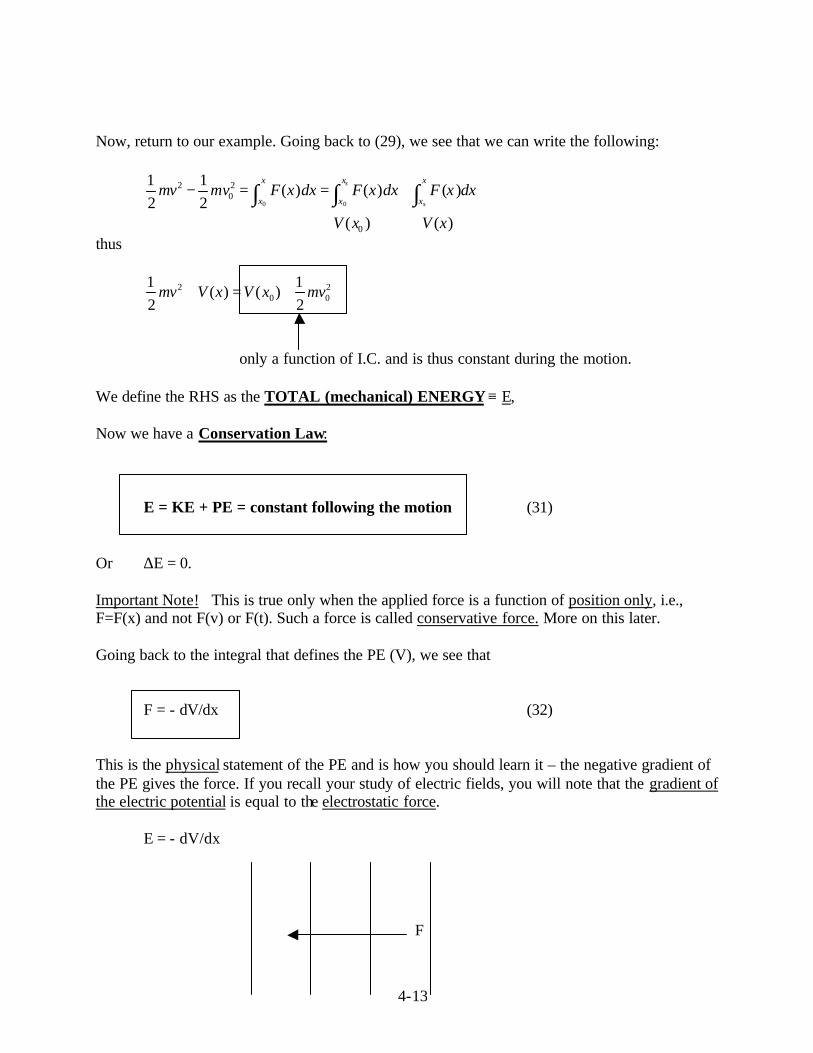
CASE I: Stable Equilibrium - If a particle or air parcel is displaced slightly, it will experience a restoring force that tends to return it to its starting location. Note that it may not return right away – but overshoot and oscillate around the initial location until it gets damped out if friction exists. The vertical location of the parcel as a function of time looks like this: If you have experienced turbulence while flying, then you have experienced the effect of stable equilibrium in the atmosphere first hand. The restoring force in the atmosphere is gravity via its role in the temperature stratification – something called static stability. The parcel oscillations result in gravity waves – we will come back to this in a little bit and derive the frequency of oscillation. For now, think physically. As you will learn in Thermodynamics, when an air parcel is lifted vertically, its surrounding pressure drops, the air parcel will expand in volume. This expansion will results in what's called the adiabatic cooling (assuming there is not heating or cooling from any other source) (the cooling happens because the air parcel has to do work to expand – based on total energy conservation, the internal energy has to decrease, therefore temperature will drop). As we will see later, the cooling happens at a more or less constant rate with height, and its called adiabatic lapse rate. The temperature of the atmosphere usually also decreases with height unless you are in a what's called inversion layer (where temperature increases – which corresponds to a very stable layer). The relative rate of temperature decrease (lapse rate) determines if the atmosphere is stable or not. Consider the following two-layered (a simplification) atmosphere, the upper layer has a lower temperature (TU) than the lower layer (TL). If we displace a parcel vertically, what will happen? It all depends on the rate at which the parcel's temperature drops relative to the rate at which the ambient temperature drops. If the parcel cools faster, then at any height above its initial level, it will be colder than the environment and will tend to sink. The restoring force is gravity! But as it
Z
t
Initial Displacement
4-17
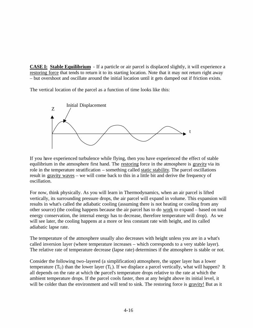
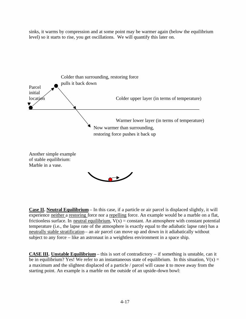
sinks, it warms by compression and at some point may be warmer again (below the equilibrium level) so it starts to rise, you get oscillations. We will quantify this later on. Parcel initial location Colder upper layer (in terms of temperature) Warmer lower layer (in terms of temperature) Another simple example of stable equilibrium: Marble in a vase. Case II. Neutral Equilibrium – In this case, if a particle or air parcel is displaced slightly, it will experience neither a restoring force nor a repelling force. An example would be a marble on a flat, frictionless surface. In neutral equilibrium, V(x) = constant. An atmosphere with constant potential temperature (i.e., the lapse rate of the atmosphere is exactly equal to the adiabatic lapse rate) has a neutrally stable stratification – an air parcel can move up and down in it adiabatically without subject to any force – like an astronaut in a weightless environment in a space ship. CASE III. Unstable Equilibrium – this is sort of contradictory – if something is unstable, can it be in equilibrium? Yes! We refer to an instantaneous state of equilibrium. In this situation, V(x) = a maximum and the slightest displaced of a particle / parcel will cause it to move away from the starting point. An example is a marble on the outside of an upside-down bowl:
Colder than surrounding, restoring force pulls it back down
Now warmer than surrounding, restoring force pushes it back up

4-18
Once you give it a push, it will keep going and never return!! In the atmosphere, this is what happens inside the thunderstorms, when an air parcel rises in an (convectively) unstable environment. Condensational heating cause the air parcel to be warmer than it's surrounding and it continues to rise, producing more condensation therefore clouds, rain, hail etc. (it will eventually hit the tropopause above which the environment becomes warmer relative to the air parcel so the environment there is stable à oscillatory motion of the air parcel starts – more on this later) It all boils down to the lapse rate of the parcel versus that of the atmosphere (in the case of saturation, it's the moist lapse rate). In this unstable situation, the so-called buoyancy force (net force between vertical pressure gradient force and gravity, more on this later) accelerates the parcel vertically. Where does the energy to perform this work come from? The CAPE (convectively available potential energy).
Warmed by condensation Cold
Warm
4-19
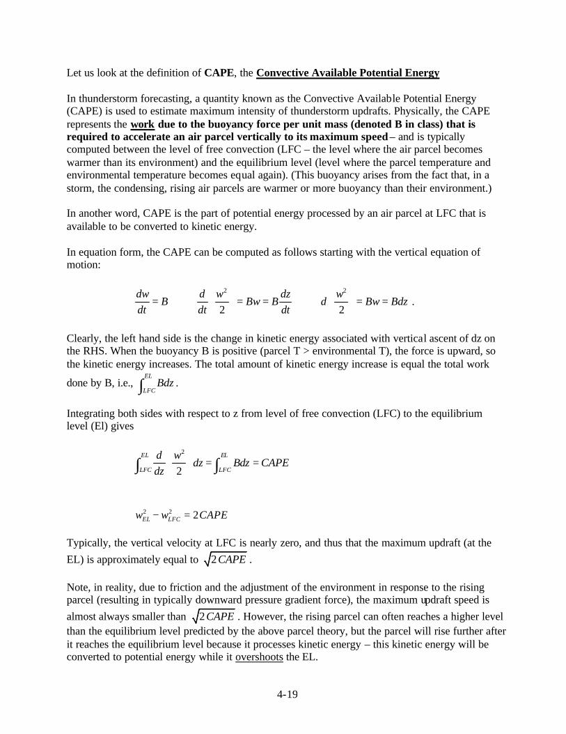
Let us look at the definition of CAPE, the Convective Available Potential Energy In thunderstorm forecasting, a quantity known as the Convective Available Potential Energy (CAPE) is used to estimate maximum intensity of thunderstorm updrafts. Physically, the CAPE represents the work due to the buoyancy force per unit mass (denoted B in class) that is required to accelerate an air parcel vertically to its maximum speed – and is typically computed between the level of free convection (LFC – the level where the air parcel becomes warmer than its environment) and the equilibrium level (level where the parcel temperature and environmental temperature becomes equal again). (This buoyancy arises from the fact that, in a storm, the condensing, rising air parcels are warmer or more buoyancy than their environment.) In another word, CAPE is the part of potential energy processed by an air parcel at LFC that is available to be converted to kinetic energy. In equation form, the CAPE can be computed as follows starting with the vertical equation of motion:
2 2
2 2dw d w dz w
B Bw B d Bw Bdzdt dt dt
= ⇒ = = ⇒ = =
.
Clearly, the left hand side is the change in kinetic energy associated with vertical ascent of dz on the RHS. When the buoyancy B is positive (parcel T > environmental T), the force is upward, so the kinetic energy increases. The total amount of kinetic energy increase is equal the total work
done by B, i.e., EL
LFCBdz∫ .
Integrating both sides with respect to z from level of free convection (LFC) to the equilibrium level (El) gives
2
2
EL EL
LFC LFC
d wdz Bdz CAPE
dz
= =
∫ ∫
2 2 2EL LFCw w CAPE− =
Typically, the vertical velocity at LFC is nearly zero, and thus that the maximum updraft (at the EL) is approximately equal to 2CAPE . Note, in reality, due to friction and the adjustment of the environment in response to the rising parcel (resulting in typically downward pressure gradient force), the maximum updraft speed is almost always smaller than 2CAPE . However, the rising parcel can often reaches a higher level than the equilibrium level predicted by the above parcel theory, but the parcel will rise further after it reaches the equilibrium level because it processes kinetic energy – this kinetic energy will be converted to potential energy while it overshoots the EL.

4-20
Soon we will go to apply all of these concepts to air parcels in the atmosphere. When we do, we will find that, under certain conditions, parcels displaced vertically in the atmosphere oscillate like springs – undergo what is called simple harmonic motion or behave as simple harmonic oscillators. Before looking at the atmospheric problem, let's review the SHO.
4.6. Simple Harmonic Oscillator This problem is simple, but is the foundation for an important phenomenon in the atmosphere – gravity waves. Consider a mass m fastened to a spring whose spring constant is k:
If we relax the spring and measure the displacement x from that state, the restoring force associated with a displacement x is F = - k x No that the key characteristics of this force is that it is directed in the opposite direction of displacement and is proportional to the amount of displacement. The more the attached objection is displaced (the spring is stretched), the larger is the force. The force is zero when the spring is not stretched. For convenience, we choose the coordinate origin so that when the spring is not stretched, the displacement x=0. The equation of motion for this system, i.e., Newton's second law, is

4-21
2
2
restoringforce
d xm F kx
dt
ma F
= = −
= =
Thus, the equation
2
2 0d x
m kxdt
+ = (34)
is the ordinary differential equation (ODE) for our system – the so-called SHO equation. If you have taken Engineering Math I, you know how to solve this equation (see separate notes on ODE). Eq. (34) can be rewritten as
0k
x xm
+ =&& (35)
where the 'dot' denotes time derivative. We just need to solve Eq.(35) to be able to tell the exact location (x) of the object at any given time (t). Being a homogeneous second-order ODE with constant coefficient, Eq.(35) always have a solution of the following form: tx X eλ= (36) where X is independent of time t and is considered the 'amplitude' of the solution. X is to be determined by the initial condition of the problem. Attention: For second-order homogenous ODE's, assuming the above solution and determining the value of parameter λ so that the solution satisfies the ODE is a STANDARD METHOD for solving such equations! If you do not understand the theory behind (as outlined in the pages on ODE's), at least remember this standard procedure! Since we consider (36) the solution of (35), it has to satisfy (35). Substituting (36) into (35) à

4-22
2 0t tkX e X e
mλ λλ + =
2( ) 0tk
X em
λλ + = (37)
To obtain nontrivial solution to (35), X cannot be zero, therefore
2 km
λ = − (38)
k
im
λ± = ± (38a)
(38) is called the characteristic equation of (35) and the solution(s) the characteristic equation is(are) called the eigenvalue(s) of the problem (see handout on linear ordinary equations). For the above problem, only when λ is equal to these eigenvalues does (36) satisfy the original ODE. Physically, the eigenvalues represent the intrinsic properties of the physical system, and often determine the frequency of oscillation, damping rate etc. For example, for the above problem, the eigenvalue is dependent on the spring constant and the mass of the particle attached. For a guitar's string, it is the length and tension of the string that determines the tune associated with this string.
Given that we found to values of λ, we have found two solutions to (35). Letting km
ω = , they
are:
1 2 and i t i tX e X eω ω− and these two solutions are linearly independent, i.e., one is not the multiple of the other. According to theories of ODE's (see handout on ODE), a solution containing two arbitrary constants to a second order ODE is the general solution to the ODE and covers all possible solutions to the ODE. We can obtain such a solution from the linear combination of the above two solutions:
1 2( ) + i t i tx t X e X eω ω−= (38b) which contains two arbitrary constants X1 and X2. No matter what there values are (can be complex number too), (38b) satisfies (35)! SO, IF YOU FOUND TWO LINEARLY INDEPENDENT SOLUTIONS TO A SECOND ORDER ODE, TO GET THE GENERAL SOLUTION, ALL YOU HAVE TO YOU IS MULTIPLING EACH BY A CONSTANT AND ADD THEM TOGETHER (CALLED LINEAR COMBINATION). You will see below that these two solutions can be put into the since and cosine form and still form a GENERAL solution!

4-23
Noting that cos sin( )ixe x i x± = ± (Euler's formula), (38b) can be rewritten as
1 2 1 2( )( ) cos( ) sin( )
2 2X X i X X
x t t tω ω+ −
= + . (38c)
Since X1 and X2 are arbitrary, the coefficients of sin() and cos() are arbitrary. They will be determined by the initial conditions of the problem anyway. It is therefore equally valid to write (38c) as
( ) cos( ) sin( )x t A t B tω ω= + (38d)
Solution (38d) still contains two arbitrary constants, A and B, and it can be verified (do it yourselves) that cos(ωt) and sin(ωt) are (independent) solutions to (35). Therefore, (38d) is the general solution to (35). We will need to determine A and B using the initial conditions now. We have mentioned initial conditions several times – initial conditions specifies the value of the dependent variables and oft en their derivatives at the start time, usually t=0, of a physical motion. For a second order ODE, we always need to initial conditions ! No surprisingly because we have two constants to determine! In the above,ω is the frequency of oscillation and has the unit of s-1. Alternatively, we can rewrite (38d) in simply and easier to understand form, by letting C = (A2 + B2 )1/2, tan θ0 = B/A, therefore
0 02 2 2 2cos( ) , sin( )
A B
A B A Bθ θ= =
+ +:
x(t) = C cos(θ0 - ωt ) (39) [ recall that cos(α+β) = cos(α)cos(β) - sin(α)sin(β)] here C and θ0 (or A and B earlier) are the two new arbitrary constants. Solution (39) is easiest to understand physically – it is pretty clear that C is the amplitude of the oscillation (which determines the range of values x(t) can have, basically from –C to C). Being a cosine function, the solution is clearly periodic in time, representing an oscillatory motion, and the

4-24
period T = ω/2π. θ0 - ωt is called the phase of oscillation and θ0 the initial phase. Clearly, x(t) = x(t+nT), where n is any integer number including zero. Eq.(35) is simple enough, it is possible to solve the equation without invoking any standard methods for ODE. Just basic integration tools are sufficient. For this alternative way, read Page 30-32 Symon's Mechanics book (section distributed). The method we used here is most general. An object whose motion follows the above simple periodic motion is called a simple harmonic oscillator. The behavior of such a SHO for different initial velocity is illustrated in the following diagram:
How can we know the above behavior from the solution obtained earlier? For case (2), the initial velocity is zero, i.e., v0(t=0) = dx/dt |t=0 = Cω sin(θ0 - ω0) =0, therefore θ0=0 à x(t) = C cos(ωt) We still need to determine C. For the same case (2), the initial position of the particle is at x(0) = x0 (the figure uses y), therefore x0 = C cos(ω0) = C. Therefore C = x0. The final solution for case (2) in the above figure is

4-25
x(t) = x0 cos(ωt)
For case (1) and (3), the initial position if x(0) = x0, therefore
x0 = C cos(θ0 - ω0) = C cos(θ0) (40a)
At t=0, there is an initial velocity of 0v± , therefore
0 0 0sin( 0) sin( )v C Cω θ ω ω θ± = − = (40b)
Solving (40a) and (40b), you get
1 00
0
tanvx
θω
− = ±
0 0
0 1 0
0
sin( )sin tan
v vC
vx
ω θω
ω−
±= =
You can see that the ± sign disappeared (canceled) from the final C formula, therefore the amplitude does not depend on the initial direction of the velocity. We can easily see why from the energy conservation position of view – at the maximum amplitude, all kinetic energy of the object is converted to the elastic potential energy which for this problem is a only a function of a the amount of spring stretching – as long as the initial kinetic energy is the same (KE does not care about the sign of velocity), the maximum realizable potential energy is the same!
In the presence of friction (acting on the object at the end of the spring), the oscillation will be damped – its amplitude will decrease with time. We will deal with this situation using atmosphere examples in the next section.

4-26
4.7. Application of SHO to the atmosphere (Read handout entitled "Hydrostatic Equilibrium") We are going to examine the "parcel method" for determining atmospheric stability. We will do both conceptual and mathematical models, and show that SHO is a key element. 4.7.1. Free vertical oscillation of an air parcel in a stable atmosphere Conceptual Analysis Assume we have an atmosphere that is hydrostatic (recall that this means – basically the gravitational force acting on a parcel is balanced by the vertical pressure gradient force so that there is no vertical acceleration), and that it has a temperature lapse rate (-dT/dz) = γ. For simplicity, we consider the atmosphere to be completely dry. So consider an atmosphere that is
Dry Hydrostatic atmosphere With constant lapse rate (-dT/dz) = γ .
Now consider a parcel of air near the ground, for example, that has the same T (temperature), p (pressure), and ρ (density) as its surroundings. Since the parcel is in a hydrostatic equilibrium (think of an object of exactly the same density as water being placed in a water tank – it should stay whatever depth it is placed at – there is zero buoyancy), it will simply "sit there" until acted upon by some external influence. Now suppose that the parcel is given a "kick" upward, e.g., by a cold front. The parcel, because it is dry, will cool at the dry adiabatic lapse rate. As you will find in your themodynamics class, the DALR, Γd = g/Cp, where Cp = specific heat for dry air at constant pressure. Assuming no heat exchange with its surrounding, the temperature in an air parcel decreases with increasing height at a dry adiabatic lapse rate of Γd = g/Cp = (-dTd/dz) The point here is that we have 2 lapse rates or rates of cooling with height: - parcel's - surrounding atmosphere's The stability of the system is based upon the relative rates of temperature change with height, i.e., the lapse rates. Let's look at some examples:
4-27
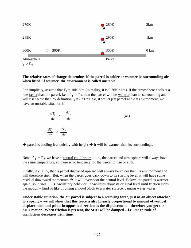
270K 280K 2km 285K 290K 1km 300K T = 300K 300K 0 km Atmosphere Parcel γ > Γd The relative rates of change determines if the parcel is colder or warmer its surrounding air when lifted. If warmer, the environment is called unstable. For simplicity, assume that Γd = 10K /km (in reality, it is 9.76K / km). If the atmosphere cools at a rate faster than the parcel, i.e., if γ > Γd, then the parcel will be warmer than its surrounding and will rise! Note that, by definition, γ = - dT/dz. So, if we let p = parcel and e = environment, we have an unstable situation if
pedTdT
dz dz − > −
(41)
pedTdT
dz dz <
à parcel is cooling less quickly with height à it will be warmer than its surroundings. Now, if γ = Γd, we have a neutral equilibrium, - i.e., the parcel and atmosphere will always have the same temperature, so there is no tendency for the parcel to rise or sink. Finally, if γ < Γd, then a parcel displaced upward will always be colder than its environment and will therefore sink. But, when the parcel goes back down to its starting level, it will have some residual downward momentum à it will overshoot the neutral level. Below, the parcel is warmer again, so it rises… à oscillatory behavior. It oscillates about its original level until friction stops the motion – kind of like throwing a wood block to a water surface, causing water waves. Under stable situation, the air parcel is subject to a restoring force, just as an object attached to a spring – we will show that this force is also linearly proportional to amount of vertical displacement and points in opposite direction as the displacement – therefore you get the SHO motion! When friction is present, the SHO will be damped – i.e., magnitude of oscillations decreases with time.

4-28
Note that the key parameter in this analysis is the dry adiabatic lapse rate – it is the rate of cooling or warming of the parcel and is fixed unless the parcel becomes saturated (i.e., the contained water vapor starts to condense due to cooling). Thus, for dry motion, one only needs to look at the environmental lapse rate, γ, to determine the stability! Quantitative Analysis We will now quantify this scenario using Newton's 2nd law applied to the atmosphere. We will take 2 points of view…, the parcel and the environment. We will first assume that there is no friction. Recall that the vertical equation of motion:
1F dVa p g
m dt ρ= = = − ∇ +
r rr r
for unit mass (m=1)
Acceleration PGF Gravity
Consider the vertical direction only, we have
1dw d dz dpg
dt dt dt dzρ = = − −
(42)
Let's use an overbar to denote quant ities associated with the environment. If we assume that the environment is hydrostatic, then the vertical acceleration is zero, so we have
10
dpg
dzρ= − − (43)
Now for the parcel, we allow for vertical acceleration, and the equation is
2
2
1d z dpg
dt dzρ= − − (44)
Now, we assume that the parcel pressure p and environmental pressure p are the same at each level, i.e., that the parcel pressure immediately adjusts to that of the environment as it rises and sinks. This is a very reasonable assumption, since the motions are slow enough for this to happen. It will not be true for supersonic flows! This doesn't violate the idea that expansion due to p difference is that causes the cooling.

4-29
If p =p at all levels, then dp dpdz dz
= as well.
Setting the two pressure gradients in (43) and (44) equal to each other gives
2
2
d zg g
dtρ ρ ρ− = − −
Solving for the vertical acceleration of the parcel gives:
2
2
d zg
dtρ ρ
ρ−
= − (45)
Often we write the density if the parcel as the sum of the environmental value ρ plus a small deviation (ρ'). Substituting, we then have
2
2
''
d zg
dtρ
ρ ρ= −
+
Since ρ' = ρ , this can be simplified
2' ' 1 ' ' ' ' '
1' 1 '/
g g g g g gρ ρ ρ ρ ρ ρ ρ
ρ ρ ρ ρ ρ ρ ρ ρ ρ ρ
− = − ≈ − − = − + ≈ − + +
In the above we used a series expansion for 1/(1+x) ≈ 1- x, and neglected the second order term in the final step. Therefore
2
2
'd zg
dtρρ
≈ − (46)
Typically, we let '
g Bρρ
− ≡ and call it parcel buoyancy à
2
2
d zB
dt= (47)
Since air density is not directly observed, in meteorology, we prefer to use temperature to measure density. Note that p =ρRT, (R is the ideal gas constant for dry air), taking a log of it à
4-30
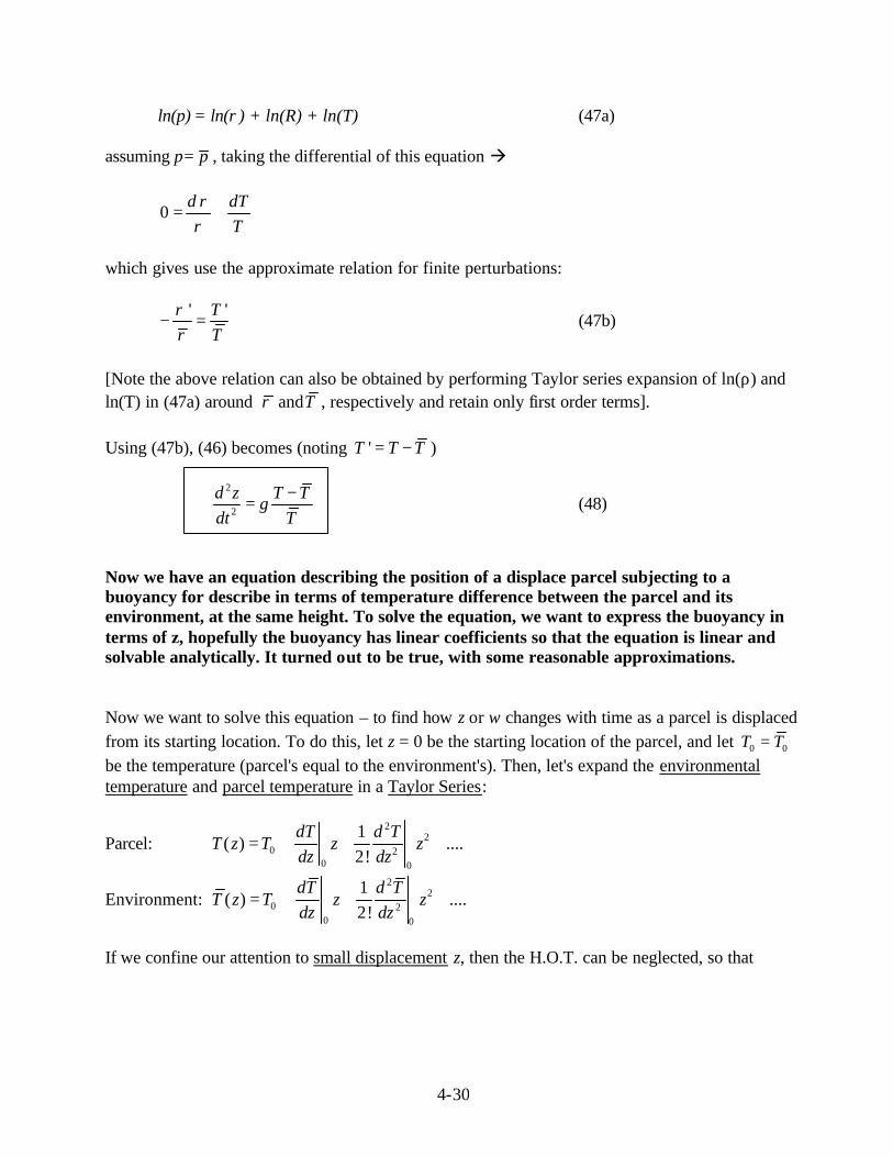
ln(p) = ln(ρ) + ln(R) + ln(T) (47a) assuming p= p , taking the differential of this equation à
0d dT
Tρ
ρ= +
which gives use the approximate relation for finite perturbations:
' 'TT
ρρ
− = (47b)
[Note the above relation can also be obtained by performing Taylor series expansion of ln(ρ) and ln(T) in (47a) around andTρ , respectively and retain only first order terms]. Using (47b), (46) becomes (noting 'T T T= − )
2
2
d z T Tg
dt T−
= (48)
Now we have an equation describing the position of a displace parcel subjecting to a buoyancy for describe in terms of temperature difference between the parcel and its environment, at the same height. To solve the equation, we want to express the buoyancy in terms of z, hopefully the buoyancy has linear coefficients so that the equation is linear and solvable analytically. It turned out to be true, with some reasonable approximations. Now we want to solve this equation – to find how z or w changes with time as a parcel is displaced from its starting location. To do this, let z = 0 be the starting location of the parcel, and let 0 0T T= be the temperature (parcel's equal to the environment's). Then, let's expand the environmental temperature and parcel temperature in a Taylor Series:
Parcel: 2
20 2
0 0
1( ) ....
2!dT d T
T z T z zdz dz
= + + +
Environment: 2
20 2
0 0
1( ) ....
2!dT d T
T z T z zdz dz
= + + +
If we confine our attention to small displacement z, then the H.O.T. can be neglected, so that

4-31
0 00
( ) ddT
T z T z T zdz
≈ + = − Γ
0 0
0
( )dT
T z T z T zdz
γ≈ + = −
Using these in (48) gives
20 0
20 0
d dT z T zd zg g z
dt T z T zγ γ
γ γ− Γ − + − Γ
= =− −
(49)
The above equation is not linear – see if it can linearized without much sacrifice to accuracy. Now let's examine the relative size of terms in the denominator 0T zγ−
T0 ~ 300 K γ ~ 5K/1000m z ~ 100 m
à 0T zγ− ~ 5
300 (100)~300 0.51000
− −
It appears as if we can neglect the γz relative to T0.
A better way of showing this is 0 0 0
1 1 1(1 / )T z T z Tγ γ
=− −
. Plugging in numbers, you can find that
0| / | 1z Tγ = . So, our expression becomes
2
20
dd zg z
dt Tγ − Γ
=
(50)
The nice thing about (50) is that the coefficient of in the equation ( g[ ] ) is constant, therefore the equation is linear! Let K = 0( ) /dg Tγ− − Γ , this is just
z Kz= −&& , (51)

4-32
or the SHO (simple harmonic oscillator) equation! Physically, what can we do with this equation? If we are given T0 and γ and the parcel lapse rate, we can find z(t) [or w(t)] à this equation actually let you predict the speed and location of air parcel! This is the simplest possible 1-D model of "dry convection" that we could imagine. And it's no more than F=ma! We have already solved equation like (51) earlier. It is ( ) cos( ) sin( )z t A K t B Kt= + (52) Note that K has units of inverse time, and thus is frequency. The associated period of oscillation is thus
T = 0 0
2 2( ) /K g T
π πγ
=− − Γ
(53)
What is this period?
1 /29.8(5.0 9.76)
2 520 ~10min320 1000
T sπ−− − = ≅ ×
So parcels displaced vertically in this situation will oscillate with a period of roughly 10 minutes. In the above, K = 0( ) /dg Tγ− − Γ measures that static stability. The larger the temperature difference between the parcel and environment (i.e., K), the stronger is the stability. The stronger is the stability, the higher is the frequency of oscillation – the oscillation is faster! When K < 0, 0dγ − Γ > , the adiabatic air parcel's temperature decreases with height slower than the environment, there T becomes higher when lifted, the air parcel should continue to rise without return. Let's see what solution we get from Eq.(51) in this case. Since K < 0, we can rewrite (510 as
| |z K z=&& the eigenvalues are therefore | |Kλ± = ± , the two solutions are therefore
| | | |1 2 and K t K tX e X e−
the first solution corresponds to an exponentially growing motion – the air parcel keep rising without return! (The general solution in this case is x(t) = | | | |
1 2 and K t K tX e X e− )

4-33
4.7.2. Damped Oscillations of an air parcel in a stable atmosphere Let's now consider the situation where the air experiences friction. As we discussed earlier, a friction force in the form of a power law is most common. Let's therefore add the term zη− & to the RHS of our parcel oscillation equation. Here, η is the drag coefficient. Now our equation of motion for the parcel is
0z z Kzη+ + =&& & . (54)
The characteristic equation (obtained by plug in a solution of the form teλ , more on this in the handout on ODE solutions) is λ2 + ηλ + K = 0, (55) thus
214
2 2K
ηλ η= − ± − . (56)
Let's define α = η/2 and β = 214
2Kη − .
λ α β± = − ± . (57) The nature of the solution depends on the roots λ. Let's examine them separately. CASE I (overdamped case): If 2 4Kη − >0, then λ will have real roots. Call them λ1 and λ2 : λ1 = - α + β
λ2 = - α - β Using our knowledge of differential equation, then solution is then ( ) ( )( ) t tz t Ae Beα β α β− − − += + (58) with the constants to be determined by the I.C. Let's look at the solution. For t > 0, both terms go to zero as to t à ∞ . Why? Because α - β > 0 (see the definition of α and β). What is the effect of the viscosity η? It appears in the exponential α ~η, so te η− à the larger the viscosity, the more rapid the decaying – i.e., the motion dies out quickly. Compare two values of η:

4-34
η t te η− 2 1 0.135 2 0.018 3 0.002 10 1 0.00005 2 2.06 x 10⁻⁹
3 9.36 x 10⁻¹⁴
The solution for CASE I is called over-damping solution – the solution is totally dominated by
te η− à no sinusoidal motion. It is illustrated below.

4-35
CASE II (damped oscillations): If η2 –4K < 0, then λ will have complex roots, i.e., β is
imaginary. Let's let β = iω where 214
2Kω η= − >0.
Then, we have λ1 = - α + iω
λ2 = - α - iω so that the general solution is ( ) [ cos( ) sin( )]tz t e A t B tα ω ω−= + (59) [which can be rewritten as 0( ) cos( )tz t Ce tα ω θ−= − where C2 = A2+B2 and tan(θ0)=B/A]. What is the physical nature of the solution? It is a damped oscillation – waves multiplied by exponential factors that damp with time since α>0. As tà∞ , z(t)à0.
4-36
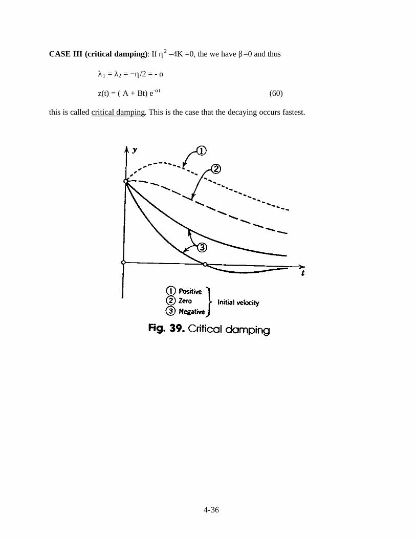
CASE III (critical damping): If η2 –4K =0, the we have β=0 and thus
λ1 = λ2 = −η/2 = - α z(t) = ( A + Bt) e-αt (60)
this is called critical damping. This is the case that the decaying occurs fastest.

4-37
5.8. Conservation of Linear Momentum: 1-D Advection Our final topic in 1-D motion involves the conservation of linear momentum. First, let's review some basic calculus and recall on an earlier discussion. In mechanics and fluid dynamics, one can view things in 2 basic ways: Lagrangian Framework – following the motion, i.e., you are riding along with an air parcel. Eulerian Framework – Here you are at a fixed location. The two can be related mathematically as follows. Suppose we have a scalar quantity F (we will apply this to vector later): F[x(t), y(t), z(t), t] Then by the chain rule of calculus, we can write the total differential as:
F F F F
dF dx dy dz dtx y z t
∂ ∂ ∂ ∂= + + +
∂ ∂ ∂ ∂. (61)
If we divide it by dt, we have
dF F dx F dy F dz Fdt x dt y dt z dt t
∂ ∂ ∂ ∂= + + +
∂ ∂ ∂ ∂ (61)
The term on the left hand side is known as the Lagrangian or material or substantial or total derivative, and it represents the total change in F following the motion of the fluid. Note that, by definition in meteorology,
/ ( )
/ ( )
dxu east west zonal wind
dtdy
v north south meridional winddtdz
w verticalmotiondt
= =
= =
= =
(62)
thus we have
dF F F F F
u v wdt t x y z
∂ ∂ ∂ ∂= + + +
∂ ∂ ∂ ∂ (63)
The LHS term is the total derivative of F (total change) following the motion because it is

4-38
0
limt
dF Fdt t∆ →
∆≡
∆ (64)
Remember that a partial derivative means the derivative of the dependent variable with respect to the specified independent variable with all other independent variables held constant. As an example, the term /F t∂ ∂ is the time rate of change in F at a fixed point (x,y,z) in space. It is also called the Eulerian derivative. Rearranging (63), we have
( ) ( ) ( )
F dF F F Fu v w
t dt x y z
a b c
∂ ∂ ∂ ∂= − + + ∂ ∂ ∂ ∂ (65)
where (a) = local derivative or Eulerian derivative (the change in F at a fixed point in space) (b) = Lagrangian derivative (the change in F following the motion of the fluid) (c) = The advection of F (including the minus sign), i.e.,
F F Fu v w
x y z ∂ ∂ ∂
− + + ∂ ∂ ∂ .
The term represents the change in F that a particle would experience if F did not vary at all with time at any fixed point, but was a function only of the 3 space coordinates. As we will see later using vectors, we can write
dF F
V Fdt t
∂= + ⋅∇
∂
r (66)
where
ˆˆ ˆ advectionvelocityV ui vj wk= + + =r
ˆˆ ˆ gradientopeartor- a vectori j kx y z
∂ ∂ ∂∇ ≡ + + =
∂ ∂ ∂ (67)
Let's look at the advection term physically for the case F = temperature (T). Look at 1-D: Assume that
0dTdt
≡ , i.e., AMA OKC

4-39
T = constant Following the motion -5 0 5 10 15 Q: What is the temperature change rate at OKC due only to advection?
42010 5 10 /
400,000
1.8 /
Tu
x
K sm
K hr
−
∂= −
∂
= − = ×
≈ −
Question: u > 0 and Tx
∂∂
> 0 à will temperature go up and down?
If T is constant following the motion of a parcel, then dT/dt = 0 à
T T
ut x
∂ ∂= −
∂ ∂
Advection is on the RHS with a minus sign! Therefore 0Tt
∂<
∂ so temperature at OKC goes down.
Reasonably because the air parcel bearing lower temperature at AMA arrived at OKC. By what physical effects could dT/dt ≠ 0 and thus modify this answer? Diabatic effects such as the sun shining (solar heating) on the ground and heating the air adjacent to it. Let's examine this more closely:
0dT T T
udt t x
∂ ∂= + =
∂ ∂ if T is conserved
following local -advection motion change As air parcel moves, its temperature might be changing by virtue of - condensation / evaporation
- radiation - turbulence - vertical motion, adiabatic cooling and warming
U=30m/s

4-40
Also, it is important to recognize that the gradients may be non-uniform and multi-dimensional. We will get to the latter when we deal with vectors. For now, let's look at the practical issue of non-uniform gradient.
Assume you are required to compute T
ux
∂−
∂over OKC with the map shown blow:
u OKC T= 0 5 10 15 20 25 This is why we draw contours on maps! It allows us to quickly estimate gradients using the spatial
scale index in the legend. In computing T
ux
∂−
∂, we want to take FINITE DIFFERENTS as an
estimate of the derivative. So, we define an increment, ∆x and write a Taylor series about OKC:
2 2
2
2 2
2
( )( ) ( ) ...
2!
( )( ) ( ) ...
2!
OKC OKC
OKC OKC
T T xT OKC x T OKC x
x x
T T xT OKC x T OKC x
x x
∂ ∂ ∆+ ∆ = + ∆ + +
∂ ∂
∂ ∂ ∆− ∆ = − ∆ + +
∂ ∂
Subtracting them gives
( ) ( )
. .2OKC
T T OKC x T OKC xH O T
x x∂ + ∆ − − ∆
= +∂ ∆
∆x ∆x OKC- ∆x OKC OKC+ ∆x This should look familiar! Go back to your Synoptic Lab I book and look up the definition of a derivative, you will see it written as

4-41
( ) ( )limx
dT T x x T xdt x∆ → ∞
+ ∆ −=
∆ (68)
which is exactly what we can write using the first Taylor series. This is exactly how numerical models computes derivatives – they put data on grids of points and then compute derivatives as finite difference, i.e., not as ∆xà0.
Bottom line: We can estimate Tx
∂∂
at OKC as
( ) ( )
2T x x T x x
x+ ∆ − − ∆
∆ (two sided finite difference)
or ( ) ( )T x x T x
x+ ∆ −
∆ (one-sided difference)
The top equation is slightly more accurate. But, what should we use for ∆x? In most cases, T will vary smoothly, except in the vicinity of fronts. It's best to take ∆x as small as possible. In our pictorial example, we might use the nearest two contours around OKC:
15 102
Tx x
∂ −≈
∂ ∆
Note that ∆x need not be uniform, i.e., it could be used as
1 2
2 1
( ) ( )T T x T xx x x
∂ −=
∂ −
What value do we use for u? Since the derivative is evaluated at OKC, we will use the wind measurement there. If the observation is missing, we might average the wind from 2 nearest stations – when these two stations are of the same distance from OKC, this average means linear interpolation! For multi-dimensional problems , the advective velocity is not always perpendicular to the temperature (or whatever field being advected) contours, in another word, not always parallel to the temperature gradient. In such cases, it is the velocity component parallel to the gradient that matters. It can be seen from the vector form of advection equation:
dF FV F
dt t∂
= + ⋅∇∂
r (69)

4-42
in which the dot product of velocity vector Vr
and gradient F∇ = n
FV
n∂∂
, where Vn is the velocity
component normal to the F contours and Fn
∂∂
is the rate of change of F in the normal direction.
Write it in another way:
F dFV F
t dt∂
= − ⋅∇∂
r (70)
The following examples show several possible scenarios: Let us assume that the variable being advected is temperature T. We examine various aspects of the advection equation and total derivative with reference to a point in space (Oklahoma City).
In the above, the isotherms, temperature gradient vector, and wind vector are shown. Assuming that the temperature is conserved following the motion, i.e., pure
advection (T
V Tt
∂= − ⋅∇
∂
r), the wind in the above example will bring in lower
values of temperature to OKC, i.e., negative advection, causing temperature at OKC to drop.

4-43
Now, because the wind is now parallel to the isotherms (perpendicular to the gradient vector), the advective change at OKC will be zero. In other words, the dot product in Eq. (69) is zero.
The temperature advection is now zero because the wind is calm! Thus, the Eulerian and Lagrangian changes in Eq.(69) are the same (zero) because the parcels are not moving.
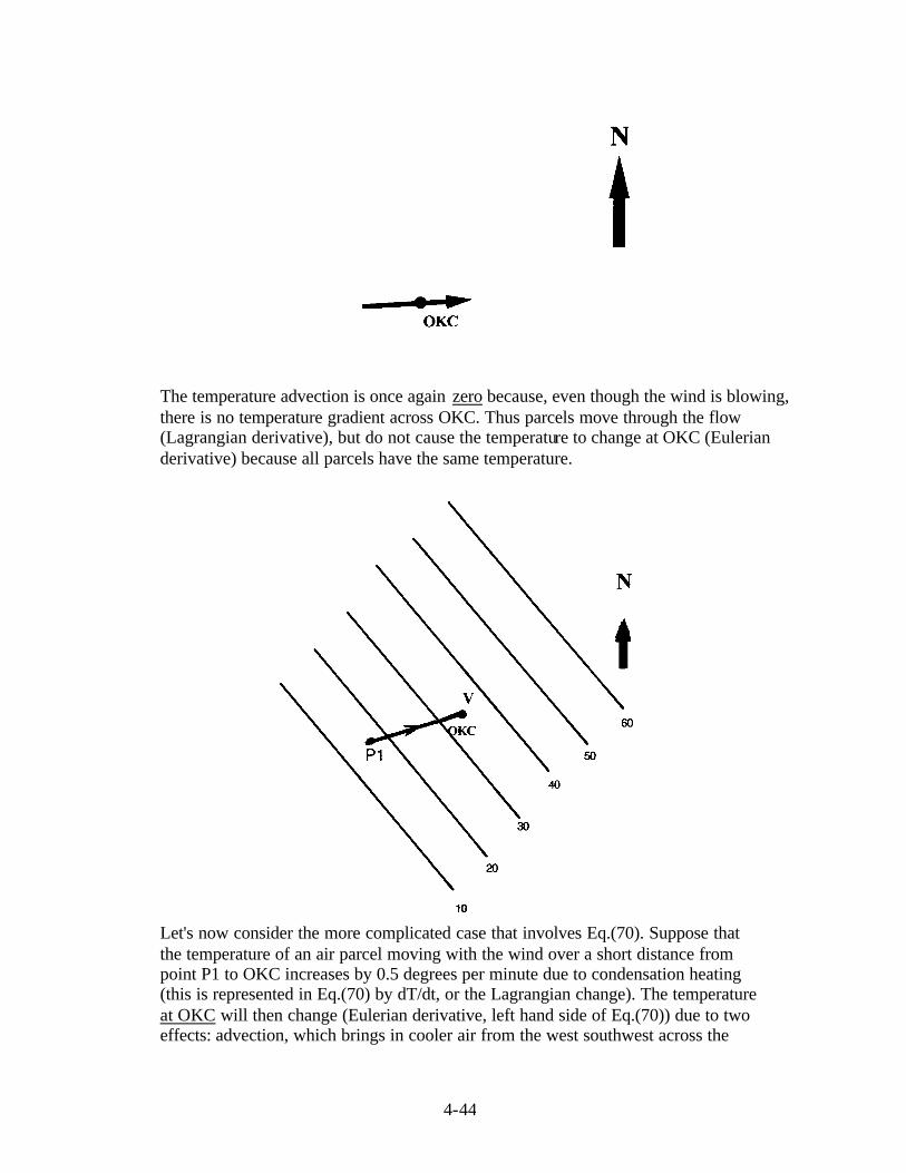
4-44
The temperature advection is once again zero because, even though the wind is blowing, there is no temperature gradient across OKC. Thus parcels move through the flow (Lagrangian derivative), but do not cause the temperature to change at OKC (Eulerian derivative) because all parcels have the same temperature.
Let's now consider the more complicated case that involves Eq.(70). Suppose that the temperature of an air parcel moving with the wind over a short distance from point P1 to OKC increases by 0.5 degrees per minute due to condensation heating (this is represented in Eq.(70) by dT/dt, or the Lagrangian change). The temperature at OKC will then change (Eulerian derivative, left hand side of Eq.(70)) due to two effects: advection, which brings in cooler air from the west southwest across the

4-45
temperature gradient, and condensational heating (dT/dt), which represents the change in the parcel's temperature as it travels along with the fluid.
Other Total Derivatives Recall that we earlier mentioned another framework for the total derivative … One moving at the speed other than that of the flow itself or a particle embedded in the flow. This is typically written
using DDt
:
DT T
C TDt t
∂= + ⋅∇
∂
r
where DDt
is the time rate of change following a particle moving at speed Cr
. This framework can
be useful when features in a physical problem are moving at different speeds – a thunderstorm, an outflow boundary, a storm chase vehicle, a rawinsonde. Only the latter might truly be moving with the horizontal wind, but you may want to compute dT/dt relative to each phenomenon or observing platform. BE SURE YOU UNDERSTAND THIESE VARISOUS DERIVATIVES AND FRAMEWORK!! Now that we understand advection, let's look at the special case where F = u:
0 ( / )u u du
u acceleration masst x dt
∂ ∂+ = = =
∂ ∂
Here, u = constant following the motion. What we see here is that, in Newton's 2nd law, the acceleration (du/dt) actually consists of 2 parts – local change + advection. What is missing? The forces.. PGF, Coriolis, etc. Adding those to the RHS is what dynamics I will be about next spring! So, let's just focus on the advection à no net force acting so F = 0 à u is constant following the motion
0u u
ut x
∂ ∂+ =
∂ ∂.
This is called the 1-D advection equation and it has some very interesting properties (also called Burger's equation). Before we look at them, let's look at some definitions:
1). If 0t
∂=
∂, the quantity being differentiated is said to be steady or steady state. It doesn't have to
be u … can be any variable. This means it doesn't very locally – at a point. Basically if you sit at this particular point, we will not see any change!

4-46
2) If 0ddt
= , the quantity being differentiated is said to be conserved following the motion. Don't
confuse this with steady state! 3) If u, v, or w is constant in space, the flow in that direction is said to uniform. The advection equation applied to u is sort of strange in that the flow is advecting itself. Let's look first at the case where the advection speed = constant = c:
0u u
ct x
∂ ∂+ =
∂ ∂.
A solution to this equation is u(x,t) = f(x-ct), e.g., sin(x-ct). Show it for yourself! f can be any differentiable function. Physically, this equation describes a wave moving right at speed c without change of shape or amplitude – all points move at the same speed. c∆t =∆x If the advection speed is now u itself, the speed of any point on the wave (advection speed) is a function of the amplitude u:
0u u
ut x
∂ ∂+ =
∂ ∂
Here, the wave steepens because it interacts with itself - this is a feedback and is nonlinear.
2
02
u ut x
∂ ∂+ = ∂ ∂
- an analytical solution is f(x-ut) – an implicit solution
The nonlinear advection terms are what make fluid dynamics and meteorology so difficult.
c c

4-47
Linear Differential Equations with Constant Coefficients Supplementary Material for Physical Mechanics 2000
The most general form of linear ordinary differential equation (ODE) of order n is
1
1 1 01( ) ( ) ... ( ) ( ) ( )n n
n nn n
d x d x dxa t a t a t a t x b t
dt dt dt
−
− −+ + + + = .
If b(t)=0, the equation is said to be homogeneous , otherwise it is inhomogeneous . The order of a differential equation is the order of the highest derivative that occurs in it. A linear differential equation is one in which there are no terms of higher than first degree in the dependent variables (in this case x) and its derivatives. Linear equations are important because there are simple general methods for solving them, especially when the coefficients are constants. Let's first look at second-order, homogeneous linear ODE's with constant coefficients as follows:
0x ax b+ + =&& & (1) where a and b are constants and a 'dot' indicates a total derivative with respective to time (it could be with respect to other independent variables).
We showed in the class that for equation 0k
x xm
+ =&& , the general solution can be written in the
form of ( ) cos( ) sin( )x t A t B tω ω= + or x(t) = C cos(θ0 - ωt ) where km
ω = . In both forms, there
are two 'arbitrary' constants A and B or C and θ0. They are called arbitrary because no matter what values are given them, the solution will satisfy the original equation. For the given phys ical problem, they are uniquely determined by the initial conditions, however. It can shown that the general solution of any second-order differential equation depends on two arbitrary conditions. It means that we can write the solution in the form x = x(t; C1, C2), such that for every value of C1 and C2, or every value within a certain range, it satisfies the equation and furthermore every solution is included in the function x(t; C1, C2). If we can find a solution containing two arbitrary constants which satisfies a second-order ODE, then we can be sure that practically every solution will be include in it. At this time, we state two theorems regarding linear homogeneous differential equations: Theorem 1: If x=x1(t) is any solution of a linear homogeneous differential equation, and C is any constant, then x=C x1(t) is also a solutuion.
4-48
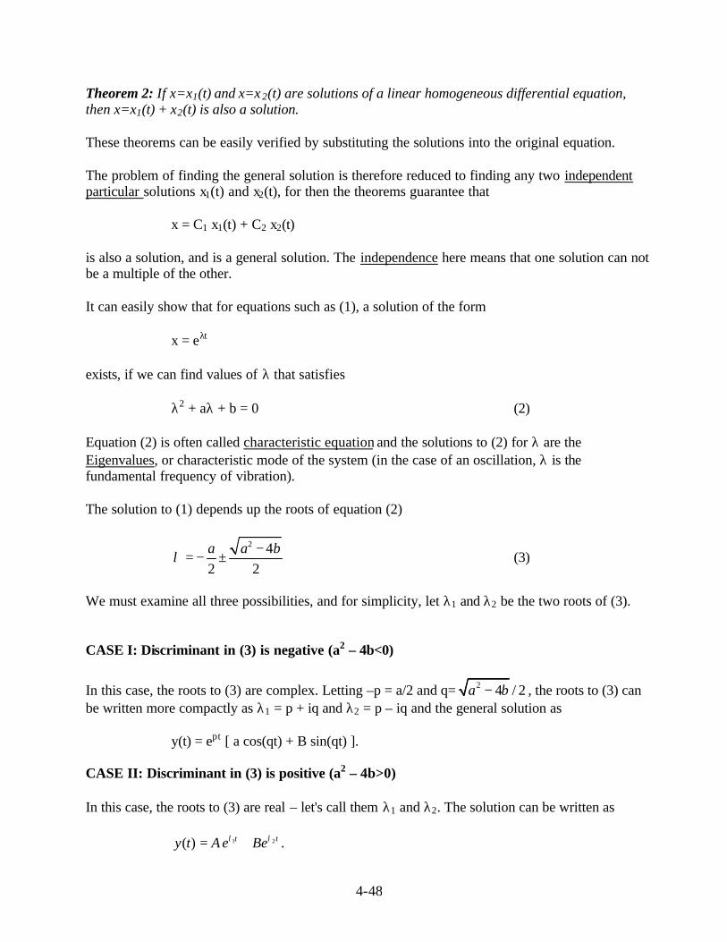
Theorem 2: If x=x1(t) and x=x 2(t) are solutions of a linear homogeneous differential equation, then x=x1(t) + x2(t) is also a solution. These theorems can be easily verified by substituting the solutions into the original equation. The problem of finding the general solution is therefore reduced to finding any two independent particular solutions x1(t) and x2(t), for then the theorems guarantee that
x = C1 x1(t) + C2 x2(t) is also a solution, and is a general solution. The independence here means that one solution can not be a multiple of the other. It can easily show that for equations such as (1), a solution of the form x = eλt exists, if we can find values of λ that satisfies
λ2 + aλ + b = 0 (2) Equation (2) is often called characteristic equation and the solutions to (2) for λ are the Eigenvalues, or characteristic mode of the system (in the case of an oscillation, λ is the fundamental frequency of vibration). The solution to (1) depends up the roots of equation (2)
2 42 2a a b
λ−
= − ± (3)
We must examine all three possibilities, and for simplicity, let λ1 and λ2 be the two roots of (3). CASE I: Discriminant in (3) is negative (a2 – 4b<0)
In this case, the roots to (3) are complex. Letting –p = a/2 and q= 2 4 / 2a b− , the roots to (3) can be written more compactly as λ1 = p + iq and λ2 = p – iq and the general solution as y(t) = ept [ a cos(qt) + B sin(qt) ]. CASE II: Discriminant in (3) is positive (a2 – 4b>0) In this case, the roots to (3) are real – let's call them λ1 and λ2. The solution can be written as
1 2( ) t ty t A e Beλ λ= + .

4-49
CASE III: Discriminant in (3) equal to zero (a2 – 4b=0) In this case, there is only one value of λ therefore we found only one solution of the form of eλt. However, it can be shown (you can easily verify yourself) that teλt is also a solution to (1) and it is independent of the first solution. Therefore we can write the general solution as
y(t) = ( A + Bt) eλt where A and B are two arbitrary constants that can be determined by the initial conditions.