CHAPTER ONECHAPTER ONEMatrices and System EquationsMatrices and System Equations

Objective:To provide solvability conditions of a linear equation Ax=b and introduce the Gaussian elimination method, a systematical approach in solving Ax=b, to solve it.

OutlineOutline

Motivative Example.Elementary row operations and Elementary M

atrices.Some Basic Properties of Matrices.Gaussian Elimination for solving Ax=b.Solvability conditions for Ax=b.

Motivative Example (curve fittingMotivative Example (curve fitting)) Given three points( )( )( ),find a

polynomial of degree 2 passing through the three given points.

Solution: Let the polynomial be

Where a,b and c are to be determined

Ax=b

11, yx 22 , yx 33, yx

cbxaxxy 2)(

c

b

a

xx

xx

xx

y

y

y

1

1

1

323

222

121

3

2

1

QuestionQuestion: Why transform to matrix : Why transform to matrix form?form?

To provide a systematic approach and to use computer resource.

QuestionQuestion: How to solve Ax=b systematically?: How to solve Ax=b systematically?

One way is to put Ax=b in triangular form,which

can be easily solved by back-substitution.

Definition: A system is said to be in triangular form if in the k-th equation the coefficients of thee first (k-1) variables are all zero and the coefficient of xk is nonzero ( k = 1,…,n)

Eg1:

4

1

2

300

420

321

3

2

1

x

x

x

43

142

232

3

32

321

x

xx

xxx

37

1

613

2

34

3

x

x

x

QuestionQuestion: How to put Ax=b in triangular form : How to put Ax=b in triangular form while leaving the solution set invariantwhile leaving the solution set invariant??

Solution: By elementary row operations as described

below.

Definition: Two systems of equations involing the same variables are said to be equivalent if they have the same solution set.

Before introducing elementary operation, we Before introducing elementary operation, we recall some definitions and notations.recall some definitions and notations.

(§ 1.3) Equality of two matrices. Multiplication of a matrix by a scalar. Matrix addition. Matrix multiplication. Identity matrix. Multiplicative inverse. Nonsingular and singular matrix. Transpose of a matrix.

Def. If and , then the

Matrix Multiplication ,

where .

Def. An (n × n) matrix A is said to be nonsingular

or invertible if there exists a matrix B such that

AB=BA=I. The matrix B is said to be a

multiplicative inverse of A. And B is denoted

by A-1.Warning: In general, AB≠BA. Matrix multiplication is not commutative.

DefinitionsDefinitions

( ) m nijA a F ( ) n r

ijB b F

( ) m rijAB C c F

1

( ,:)n

ij j ik kjk

c a i b a b

Def. The transpose of an (m × n) matrix A is the (n ×

m) matrix B defined by for j=1,…,n and

i=1,…,m. The transpose of A is denoted by AT.

Def. An (n × n) matrix A is said to be symmetric if AT=A .

Definitions (cont.)Definitions (cont.)

ji ijb a

Some Matrix PropertiesSome Matrix Properties

Let be scalars,A,B and C be matrices

with proper dimensions.

(Commutative Law)

(Associative Law)

(Associative Law)

(Distributive Law)

(Distributive Law)

&

BCACCBA

ACABCBA

BCACAB

CBACBA

ABBA

)(

)(

)()(

)()(

TTT

TT

TT

BABA

AA

AA

BABA

AAA

BABAAB

AA

)(

)(

)(

)(

)(

)()()(

)()(

111)(

)(

ABAB

ABAB TTT

Some Matrix Properties (cont.)Some Matrix Properties (cont.)

NotationsNotations

,

The matrix is called an

augmented matrix.

In general, or .

n

n

nm

mnm

n

F

x

x

X

F

aa

aa

A

1

1

111

m

m

F

b

b

b

1

mmnm

n

baa

baa

bA

1

1111

F CF

Moreover,we define

1

1

( ,:)

(:, )

i in

j

j

mj

a i a a

a

a a j

a

1 2,

1

(1,:)

,

( ,:)

(1,:)

( ,:)

n

n

i ii

a

A a a a

a m

a x

Ax x a

a n x

Def: Let and .Then

is said to be a linear combination of .

Note that .We have the next result.

Theorem1.3.1: Ax=b is consistent b can be written

as a linear combination of colum vectors

of A.

1 2a ,a ,..., a nn F

1 2c ,c ,..., cn F1

am

i ii

c

i iAx x a

1 2a ,a ,..., an

Application 1: Weight ReductionApplication 1: Weight Reduction

Table 1

Calories Burned Per HourWeight in lb

Exercise Activity 152 161 170 178

Walking 2 mph 213 225 237 249

Running 5.5 mph 651 688 726 764

Bicycling 5.5mph 304 321 338 356

Tennis 420 441 468 492

Application 1: Weight Reduction (cont.)Application 1: Weight Reduction (cont.)

Table 2

Hours Per Day For Each ActivityExercise schedule

walking Running Bicycling Tennis

Monday 1.0 0.0 1.0 0.0

Tuesday 0.0 0.0 0.0 2.0

Wednesday 0.4 0.5 0.0 0.0

Thursday 0.0 0.0 0.5 2.0

Friday 0.4 0.5 0.0 0.0

Application 1: Weight Reduction Application 1: Weight Reduction (end)(end)

Solution:

1.0 0.0 1.0 0.0 605249

0.0 0.0 0.0 2.0 984764

0.4 0.5 0.0 0.0 481356

0.0 0.0 0.5 2.0 1162492

0.4 0.5 0.0 0.0 481.6

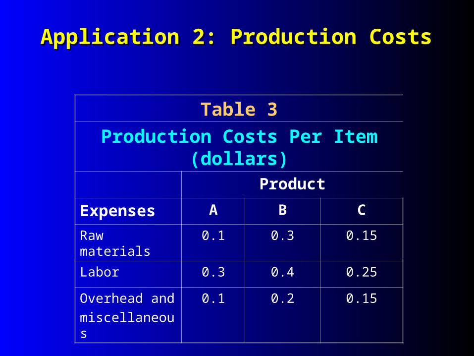
Application 2: Production CostsApplication 2: Production Costs

Table 3

Production Costs Per Item (dollars)Product

Expenses A B C

Raw materials 0.1 0.3 0.15

Labor 0.3 0.4 0.25

Overhead and

miscellaneous

0.1 0.2 0.15

Application 2: Production Costs (cont.)Application 2: Production Costs (cont.)

Table 4

Amount Produced Per QuarterSeason

Product Summer Fall Winter Spring

A 4000 4500 4500 4000

B 2000 2600 2400 2200

C 5800 6200 6000 6000

Application 2: Weight Reduction (cont.)Application 2: Weight Reduction (cont.)

Solution:0.1 0.3 0.15

0.3 0.4 0.25

0.1 0.2 0.15

M

4000 4500 4500 4000

2000 2600 2400 2200

5800 6200 6000 6000

P

Application 2: Weight Reduction (cont.)Application 2: Weight Reduction (cont.)

Solution:

1870 2160 2070 1960

3450 3940 3810 3580

1670 1900 1830 1740

MP

Application 2: Production Costs Application 2: Production Costs (end)(end)

Table 5

Amount Produced Per QuarterSeason

Summer Fall Winter Spring Year

Raw materials 1,870 2,160 2,070 1,960 8,060

Labor 3,450 3,940 3,810 3,580 14,780

Overhead and miscellaneous

1,670 1,900 1,830 1,740 7,140

Total production cost

6,990 8,000 7,710 7,280 29,980

Solution:

Application 5: Networks and Graphs (P.57)Application 5: Networks and Graphs (P.57)

Application 5: Networks and Graphs Application 5: Networks and Graphs (cont.)(cont.)

n nIf A is a F ,

1 , if { , } is an edge of the graph.then

0 , if there is no edge joioning and .

i j

iji j

adjacency matrix

V Va

V V

for Figure 1.3.2,

0 1 0 0 0

1 0 0 0 1

adjacency matrix 0 0 0 1 1

0 0 1 0 1

0 1 1 1 0

A

DEF.

Application 5: Networks and Graphs Application 5: Networks and Graphs (end)(end)

3

0 2 1 1 0

2 0 1 1 4

1 1 2 3 4

1 1 3 2 4

0 4 4 4 2

A

Theorem 1.3.3. If A is an n × n adjacency matrix of a graph and represents the ijth entry of Ak, then is equal to the number of walks of length from to Vi to Vj.

( ) kija

( ) kija

Application 6: Information Retrieval (P.59)Application 6: Information Retrieval (P.59)

Suppose that our database, consists of these book titles:

B1. Applied Linear AlgebraB2. Elementary Linear AlgebraB3. Elementary Linear Algebra with ApplicationsB4. Linear Algebra and Its ApplicationsB5. Linear Algebra with ApplicationsB6. Matrix Algebra with ApplicationsB7. Matrix Theory

The collection of key words is given by the following alphabetical list：

algebra, application, elementary, linear, matrix, theory

Application 6: Information Retrieval (cont.)Application 6: Information Retrieval (cont.)

Table 8Array Representation for

Database of Linear Algebra Books

Books

Key Words B1 B2 B3 B4 B5 B6 B7

algebra 1 1 1 1 1 1 0

application 1 0 1 1 1 1 0

elementary 0 1 1 0 0 0 0

linear 1 1 1 1 1 0 0

matrix 0 0 0 0 0 1 1

theory 0 0 0 0 0 0 1

Application 6: Information Retrieval Application 6: Information Retrieval (end)(end)

If the words we are searching for are applied, linear, and algebra,then the database matrix and search vector are given by

1 1 1 1 1 1 0 1

1 0 1 1 1 1 0 1

0 1 1 0 0 0 0 0

1 1 1 1 1 0 0 1

0 0 0 0 0 1 1 0

0 0 0 0 0 0 1 0

A x

1 1 0 1 0 0 31

1 0 1 1 0 0 21

1 1 1 1 0 0 30

1 1 0 1 0 0 31

1 1 0 1 0 0 30

1 1 0 0 1 0 20

0 0 0 0 1 1 0

y

If we set y= ATx, then

Let’s back to solve Ax=bLet’s back to solve Ax=b Eg2

432

13

32

321

321

321

xxx

xxx

xxx

20

10670

32

32

32

321

xx

xx

xxx

7

4

7

1

1067

32

3

32

321

x

xx

xxx

4132

1113

3321

2110

10670

3121

7

4

7

100

10670

3121

(§ 1.2)

Three types of Elementary row operations.

I. Interchange two row.

II. Multiply a row by .

III. Replace a row by its sum with a multiple of

another row.

0\

Lead variables and free variables(p.15)Eg:

, and are lead variables while and

are free variables.

510000

223100

102021

3x1x 5x

4x

2x

Def. A matrix is said to be in row echelon form if

(i) The first nonzero entry in each row is 1.

(ii) If row k does not consist entirely of zero,

the number of leading zero entries in row

k+1 is grater then the number of leading

zero entries in row k.

(iii) If there are rows whose entries are all zero, they

are below the rows having nonzero entries.

Def. The process of using row operations I, II, and III to

transform a linear system into one whose augmented

matrix is in row echelon form is called Gaussian

elimination.

Def. A linear system is said to be overdetermined

if there are more equations(m) than unknowns

(n). (m > n) Warning: Overdetermined systems are usually (but not always) in consistent.

Def. A system of m linear equations in n unknowns

is said to be underdetermined if there are

fewer equations. (m < n)

Overdetermined and UnderdeterminedOverdetermined and Underdetermined

Def. A matrix is said to be in reduced row echelon

form if:

(i) The matrix is in row echelon form.

(ii) The first nonzero entry in each row is the

only nonzero entry in its column.

Def. The process of using elementary row operations

to transform a matrix into reduced row echelon

form is called Gauss-Jordan reduction.

Reduced Row Echelon FormReduced Row Echelon Form

Application 2: Electrical Networks (P.22)Application 2: Electrical Networks (P.22)

Application 2: Electrical Networks Application 2: Electrical Networks (end)(end)

Kirchhoff’s Laws: 1. At every node the sum of the incoming currents equals the sum of the outgoing currents. 2. Around every closed loop the algebraic sum of the voltage must equal the algebraic sum of the voltage drops.

1 1 1 01 1 1 0

2 41 1 1 0 0 1

3 34 2 0 8

0 0 1 10 2 5 9

0 0 0 0

Application 4: Economic Models For Application 4: Economic Models For Exchange of Goods Exchange of Goods (P.25)(P.25)

F

M

C

1/2

1/4

1/4

F M C

1/3

1/3

1/3

1/2

1/4

1/4

(§ 1.4)(§ 1.4) Elementary MatricesElementary Matrices

Type I ( ): Obtained by interchanging rows i and j

from identity matrix.

Type II ( ): Obtained from identity matrix by

multiplying row i with .

Type III ( ): Obtained from identity matrix by adding

to row j.

ijE

)(iE

)(ijE

irow

means performing type I row operation on A. means performing type II row operation on A. means performing type III row operation on A.

means performing type I column operation on A. means performing type II column operation on A. means performing type III column operation on A.

AEij

AEi )(AEij )(

ijAE

( )iAE ( )ijAE

Elementary Row / Column OperationElementary Row / Column Operation

Theorem1.4.2:

If E is an elementary matrix, then E is nonsingular and E-1 is an elementary matrix of the same type.

With

The solution set of a linear equations is invariant under th

ree types row operation. and have the solution set.

)()(

)/1()(1

1

1

ijij

ii

ijij

EE

EE

EE

Ax b

EAx Eb

Def. A matrix B is row equivalent to A if there exists a

finite sequence of elementary matrices such that

Row Equivalent Row Equivalent (P.71)(P.71)

1 2, ,..., kE E E

1 1...k kB E E E A

Theorem1.4.3

(a) A is nonsingular.

(b) Ax=0 has only the trivial solution 0.

(c) A is row equivalent to I.

(a) (b) Let be a solution of Ax=0.

(b) (c) Let A ~ U, where U is in reduced row echelon form. Suppose U contains a zero row. by Th1.2.1, Ux=0 has a nontrivial solution thus A~I.

(c) (a)

A~I A= E1 …… Ek for some E1 … Ek

∵ each Ei is nonsingular. ∴ A is nonsingular. (by Th.1.2.1)

row

0x1 1 1

0 0 0( ) ( ) 0 0x A A x A Ax A

Proof of Theorem 1.4.3

Corollary1.4.4Corollary1.4.4 Ax=b has a unique solution A is nonsingular.Ax=b has a unique solution A is nonsingular.

Pf: " “ The unique solution is .

" " Suppose is the unique solution and A is

singular.

is also a solution of Ax=b.

A is nonsingular.

bAx 1

x̂

^^

^

)(

00

xZx

bZxA

AZZ

3.4.1Th

BUT in general, and AB=AC B=C.

Eg.

Moreover,AC=AB while .

01

01A

10

10B

11

10C

01

01

10

10BAAB

CB

AB6=BA

If A is nonsingular and row equivalent to I, so

there exists elementary matrices such that

then,

EEkk……EE11(A | I)= ((A | I)= (EEkk……EE11‧‧A | A | EEkk……EE11‧‧I) I) ( by )

= (I | = (I | EEkk……EE11‧‧I) I) ( by )

= (I | A= (I | A-1-1))

1 1

-11 1

... A = I ---------- 1

... = A ---------- 2

k k

k k

E E E

E E E I

1

2

Method For Computing

Q: Compute A-1 if .

Sol:

Example 4. (P.73)

1 4 3

1 2 0

2 2 3

A

1 4 3 1 0 0

1 2 0 0 1 0

2 2 3 0 0 1

A

1 1 11 0 0

2 2 21 1 1

0 1 04 4 41 1 1

0 0 16 2 6

A

1 1 1

2 2 21 1 1

4 4 41 1 1

6 2 6

A

Q: Compute A-1 if .

Sol:

Example 4. (cont.)

1 4 3

1 2 0

2 2 3

A

1 4 3 1 0 0

1 2 0 0 1 0

2 2 3 0 0 1

A

1 1 11 0 0

2 2 21 1 1

0 1 04 4 41 1 1

0 0 16 2 6

A

1 1 1

2 2 21 1 1

4 4 41 1 1

6 2 6

A

Diagonal and Triangular Matrices

Def. An n × n matrix A is said to be upper triangular if aij=0 for i > j and lower triangular if aij=0 for i > j.

Def. An n × n matrix B is diagonal if aij=0 whenever i ≠ j.

Triangular Factorization

If an n × n matrix C can be reduced to upper triangular form

using only row operation III, then C has an LU factorization.

The matrix L is unit lower triangular, and if i > j, then lij is the multiple of t he jth row subtracted from the ith row during the reduction process.

Example 6. (P.74)

2 4 2

1 5 2

4 1 9

A

1 0 0

11 0

22 3 1

2 4 2

0 3 1

0 0 8

L

U

row operation III

Mark:

2 4 2

1 5 2

4 1 9

LU A

Let A be an m × n matrix and B is an n × r matrix.

It is often useful to partition A and B and express the

product in terms of the submatrices of A and B.

In general, partition B into columns

then

partition A into rows , then

Block Multiplication

1( ,..., )rb b

1 2( , ,..., )rAB Ab Ab Ab

(1,:)

(2,:)

( ,:)

a

aA

a m

(1,:)

(2,:)

( ,:)

a B

a BAB

a m B

Case 1.

Case 2.

Case 3.

Block Multiplication (cont.)

1 2 1 2A B B AB AB

1 1

2 2

A ABB

A A B

11 2 1 1 2 2

2

BA A AB A B

B

Case 4.

Let

then

Block Multiplication (cont.)

11 1 11 1

1 1

and B t r

s t t r

s st t tr

A A B B

A F F

A A B B

11 1

11

, where r t

s rij ik kj

ks sr

C C

AB C F C A B

C C

Example 2. (P.85)

Let A be an n × n matrix of the form ,

where A11 is a k × k matrix (k < n ) . Show that A is nonsingular if and only if A11 and A22 are nonsingular.

11

22

A OA

O A

Solution:

Give two vectors ,

This product is referred to as a scalar product or an

inner product.

Scalar / Inner Product

and in nx y R

1

2 1 11 2 1 1 2 2( , ,..., ) T

n n n

n

y

yx y x x x x y x y x y R

y

Give two vectors ,

The product is referred to as the outer product

of .

Outer Product

and in nx y R

1 1 1 1 2 1

2 2 1 2 2 2 1 2

1 2

( , ,..., )

n

nT n nn

n n n nn

x x y x y x y

x x y x y x yxy y y y R

x y x y x yx

Txy

and x y

Suppose that , then

This representation is referred to as an outer product

expansion .

Outer Product Expansion

and m n k nX F Y F

1

21 2 1 11 2 2( , ,..., )

T

TT T T T

n n n

Tn

y

yXY x x x x y x y x y

y