chapter two supply and demand. © 2007 pearson addison-wesley. all rights reserved.2–2 supply and...

Chapter Two

Supply and Demand

© 2007 Pearson Addison-Wesley. All rights reserved. 2–2

Supply and Demand

• In this chapter, we examine six main topics.– Demand– Supply – Market equilibrium– Shocking the equilibrium– Effects of government interventions– When to use the supply-and-demand

model


Demand

• Potential consumers decide how much of a good or service to buy on the basis of its price and many other factors, including their own tastes, information, prices of other goods, incomes, and government actions.


The Demand Curve

• Quantity demanded– The amount of a good that consumers are

willing to buy at a given price, holding constant the other factors that influence purchases

• Demand curve– The quantity demanded at each possible

price, holding constant the other factors that influence purchases


Figure 2.1 A Demand Curve

200 220

Demand curve for pork, D1

240 286Q, Million kg of pork per year

0

2.303.30

4.30

14.30


The Demand Curve

• One of the most important things to know about a graph of a demand curve is what is not shown. All relevant economic variables that are not explicitly shown on the demand curve graph — tastes, information, prices of other goods (such as beef and chicken), income of consumers, and so on —are hold constant.


Effect of Prices on the Quantity Demanded

• Many economists claim that the most important empirical finding in economics is the Law of Demand: Consumers demand more of a good the lower its price, holding constant tastes, the prices of other goods, and other factors that influence the amount they consume. According to the Law of Demand, demand curves slope downward, as in Figure 2.1.


Effect of Other Factors on Demand

• Economists use a simpler approach to show the effect on demand of a change in a factor that affects demand other than the price of the good. A change in any factor other than price of the good itself causes a shift of the demand curve rather than a movement along the demand curve.


Figure 2.2 A Shift of A Demand Curve

220176

Effect of a 60¢ increase in the price of beef

D1

D2

232Q, Million kg of pork per year

0

3.30


The Demand Function

• In addition to drawing the demand curve, you can write it as a mathematical relationship called the demand function. The processed pork demand function is

Q ＝ D (p, pb, pc, Y), (2.1) where Q is the quantity of pork demanded, p

is the price of pork, pb is the price of beef, pc is the price of chicken, and Y is the income of consumers.


Summing Demand Curves• We can use the demand functions to determine the

total demand of several consumers. Suppose that the demand function for Consumer 1 is

Q1 ＝ D1(p) and the demand function for Consumer 2 is

Q2 ＝ D2(p)

At price p, Consumer 1 demand Q1 units, Consumer 2 demands Q2 units, and the total demand of both consumers is the sum of the quantities each demands separately:

Q ＝ Q1 ＋ Q2 ＝ D1(p) ＋ D2(p)

We can generalize this approach to look at the total demand for three or more consumers.


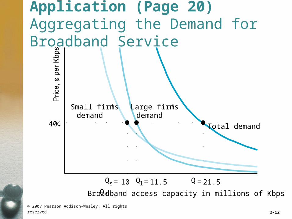
Qs = 10 Q = 21.5Q, Broadband access capacity in millions of Kbps

Large firms’ demand

Small firms’ demand

Total demand

Ql = 11.5

40¢

Application (Page 20) Aggregating the Demand for Broadband Service


Supply

• Firms determine how much of a good to supply on the basis of the price of that good and other factors, including the costs of production and government rules and regulations. Usually, we expect firms to supply more at a higher price.


The Supply Curve

• Quantity supplied– The amount of a good that firms want to

sell at a given price, holding constant other factors that influence firms’ supply decisions, such as costs and government actions

• Supply curve– The quantity supplied at each possible

price, holding constant the other factors that influence firms’ supply decisions


Figure 2.3 A Supply Curve

220176

Supply curve, S1


0

3.30

5.30


Effect of Price on Supply

• The supply curve for pork is upward sloping. As the price of pork increases, firms supply more.

• An increase in the price of pork causes a movement along the supply curve, resulting in more pork being supplied.


Effect of Other Variable on Supply

• A change in a variable other than the price of pork causes the entire supply curve to shift.

• It is important to distinguish between a movement along a supply curve and a shift of the supply curve.


Figure 2.4 A Shift of a Supply Curve

205176

Effect of a 25¢ increase in the price of hogs

S1S2


0

3.30


The Supply Function

• We can write the relationship between the quantity supplied and price and other factors as a mathematical relationship called the supply function. Written generally, the processed pork supply function is

Q ＝ S (p, ph) (2.5)

where Q is the quantity of processed pork supplied, p is the price of processed pork, and ph is the price of a hog.


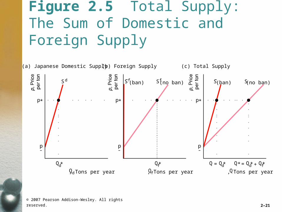
Summing Supply Curves

• The total supply curve shows the total quantity produced by all suppliers at each possible price. For example, the total supply of rice in Japan is the sum of the domestic and foreign supply curves of rice.


Figure 2.5 Total Supply: The Sum of Domestic and Foreign Supply

Qd*

Sd S f (ban)

Qf* Q = Qd* Q* = Qd* + Qf*Qd, Tons per year Qf , Tons per year Q, Tons per year

(a) Japanese Domestic Supply (b) Foreign Supply (c) Total Supply

p* p* p*

– S (ban)– S (no ban)S f (no ban)

p–

p–

p–


Page 26 Solved Problem 2.2

Sd

Q, Tons per year

(a) U.S. Domestic Supply (b) Foreign Supply (c) Total Supply

p* p* p*

p– p– p–

S–

S

Qd– Qf

–

Qd, Tons per year Qf , Tons per year

Qd* Qf*

S f–

S f

Qd* + Qf*–Qd* + Qf

––Qd + Qf


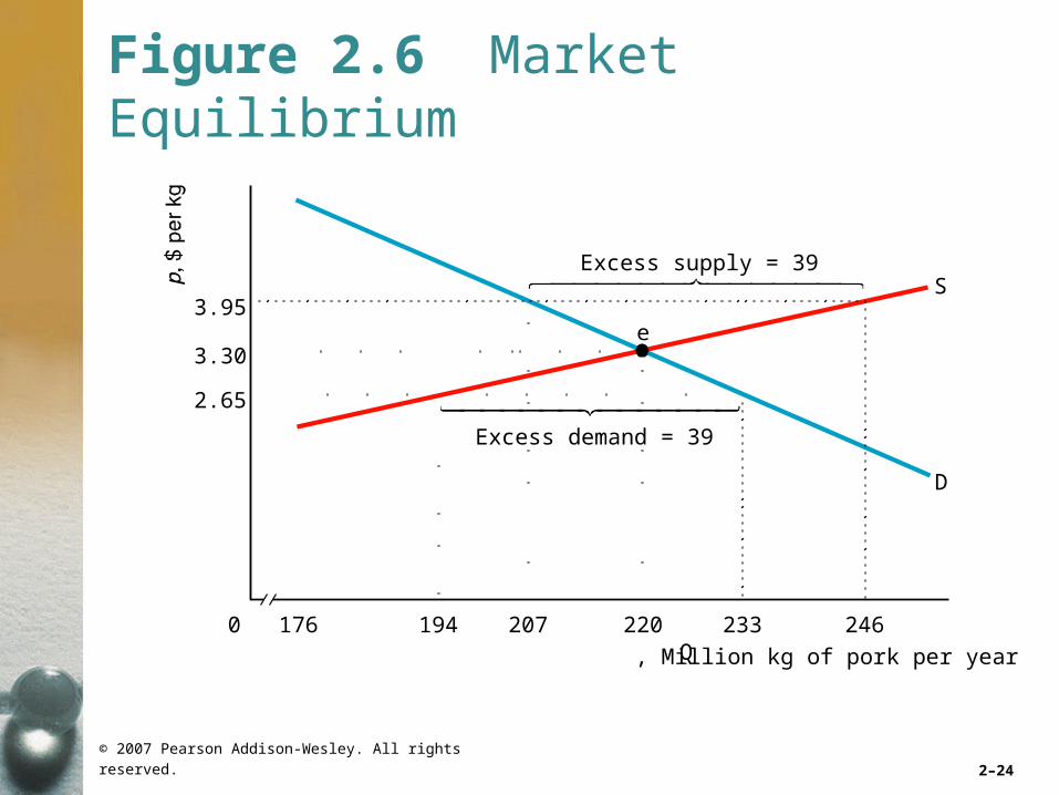
Market Equilibrium

• When all traders are able to buy or sell as much as they want, we say that the market is in equilibrium: a situation in which no participant wants to change its behavior. A price at which consumers can buy as much as they want and sellers can sell as much as they want is called an equilibrium price. The quantity that is bought and sold at the equilibrium price is called equilibrium quantity.


Figure 2.6 Market Equilibrium

220176

D

S

e

233 246194 207Q, Million kg of pork per year

0

3.95

3.30

2.65

Excess supply = 39

Excess demand = 39


Using Math to Determine the Equilibrium• We use the supply and demand functions to solve for

the equilibrium price at which the quantity demanded equals supplied (the equilibrium quantity). The demand function, Equation 2.3, shows the relationship between the quantity demanded, Qd, and the price:

Qd ＝ 286 － 20p

• The supply function, Equation 2.7, tells us the relationship between the quantity supplied, Qs, and the price:

Qs ＝ 88 ＋ 40p

We want to find the p at which Qd ＝ Qs ＝ Q, the equilibrium quantity.


Forces That Drive the Market to Equilibrium

• A market equilibrium occurs without any explicit coordination between consumers and firms. In a competitive market such as that for agricultural goods, millions of consumers and thousands of firms make their buying and selling decisions independently. Yet each firm can sell as much as it wants; each consumer can buy as much as he or she wants. It is as though an unseen market force, like an invisible hand, directs people to coordinate their activities to achieve a market equilibrium.



• Excess demand– The amount by which the quantity

demanded exceeds the quantity supplied at a specified price

• Excess supply– The amount by which the quantity supplied

is greater than the quantity demanded at a specified price



• At any price other than the equilibrium price, either consumers or suppliers are unable to trade as much as they want. These disappointed people act to change the price, driving the price to the equilibrium level.


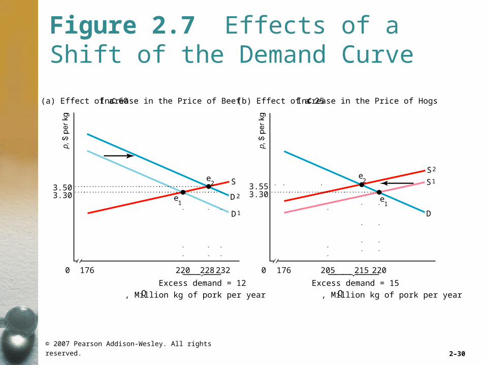
Shocking the Equilibrium

• The equilibrium changes only if a shock occurs that shifts the demand curve or the supply curve. These curves shift if one of the variables we were holding constant changes.


Figure 2.7 Effects of a Shift of the Demand Curve

D1

D2

S1

S2

S

1760 220 228 232

Q, Million kg of pork per year

Excess demand = 12Q, Million kg of pork per year

3.303.50

3.303.55

e2

e1 e

1

e2

D

(a) Effect of a 60¢ Increase in the Price of Beef (b) Effect of a 25¢ Increase in the Price of Hogs

1760 220205 215

Excess demand = 15


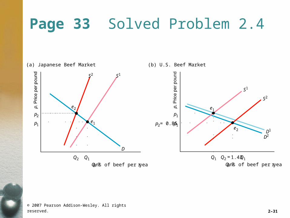
Page 33 Solved Problem 2.4

Q, Tons of beef per year

p2

p1

S1

D

S2

e1

e2

Q2 Q1

(a) Japanese Beef Market

Q, Tons of beef per year

p1

p2 = 0.85p1

S1

D1

D2

S2

e1

e2

Q1 Q2 = 1.43Q1

(b) U.S. Beef Market


Effects of Government Interventions

• A government can affect a market equilibrium in many ways. Sometimes government actions cause a shift in the supply curve, the demand curve, or both curves, which causes the equilibrium to change. Some government interventions, however, cause the quantity demanded to differ from the quantity supplied.


Policies That Shift Supply Curves

• The Japanese government’s ban on rice imports raised the price of rice in Japan substantially.

• The ban has no effect on demand if Japanese consumers do not care whether they eat domestic or foreign rice. The ban causes the total supply curve to rotate toward the origin from S (total supply is the horizontal sum of domestic and foreign supply) to S (total supply equals the domestic supply).


Figure 2.8 A Ban on Rice Imports Raises the Price in Japan

Q2

Q1

S (no ban)

D

Q, Tons of rice per year

p2

e2

e1

p1

S (ban)–


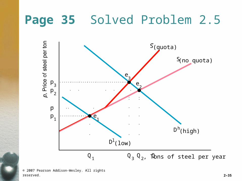
Solved Problem 2.5

Q2

Q3

Dh (high)

Q1

S (no quota)

Q, Tons of steel per year

p2

p3 e

2

e3

e1

p1

S (quota)–

p–

Dl (low)


Policies That Cause Demand to Differ From Supply

• Some government policies do more than merely shift the supply or demand curve. For example, governments may control prices directly, a policy that leads to either excess supply or excess demand if the price the government sets differs from the equilibrium price.


Price Ceilings

• Price ceilings have no effect if they are set above the equilibrium price that would be observed in the absence of the price controls.

• However, if the equilibrium price, p, would be above the price ceiling p, the price that is actually observed in the market is the price ceiling.

• As a result, an enforced price ceiling causes a shortage: a persistent excess demand.


Figure 2.9 Price Ceiling on Gasoline

Qs Q2

Q1 = Qd

Price ceiling

S1

D

S 2

Q, Gallons of gasoline per monthExcess demand

p2

e2

e1

p1 = p–


Price Floors• Governments also commonly use price

floors. One of the most important examples of a price floor is the minimum wage in labor markets. The minimum wage law forbids employers from paying less than the minimum wage, w.

• If the minimum wage binds—exceeds the equilibrium wage, w*—the minimum wage creates unemployment, which is a persistent excess supply of labor.


Figure 2.10 Minimum Wage

Ld L* Ls

Minimum wage, price floor

S

D

L, Hours worked per year

Unemployment

ew*

w—


Why Supply Need Not Equal Demand

• The price ceiling and price floor examples show that the quantity supplied does not necessarily equal the quantity demanded in a supply-and-demand model.

• Because we define the quantities supplied and demanded in terms of people’s wants and not actual quantities bought and sold, the statement that “supply equals demand” is a theory, not merely a definition. This theory says that the equilibrium price and quantity in a market are determined by the intersection of the supply curve and the demand curve if the government does not intervene.


When to Use the Supply-and-Demand Model

• Supply-and-demand theory can help us to understand and predict real-word events in many markets. In this semester, we discuss competitive markets in which the supply-and-demand model is a powerful tool for predicting what will happen to market equilibrium if underlying conditions—tastes, incomes, and prices of inputs—change.


When to Use the Supply-and-Demand Model

• This model is applicable in markets in which:– Everyone is a price taker– Firms sell identical products– Everyone has full information about the

price and quality of goods– Costs of trading are low

Markets with these properties are called perfectly competitive markets.

chapter two supply and demand. © 2007 pearson addison-wesley. all rights reserved.2–2 supply and...

Documents

demand slide

demand economists

law of demand

demand functions

total demand

demand curve quantity

purchases demand curve

demand model slide