chapter1 a review of probability and stochastic processes · 2 1 a review of probability and...
TRANSCRIPT

Chapter 1
A Review of Probability and Stochastic
Processes
The seminal studies about probability go back to the 17th century with Blaise
Pascal (1623–1662), Pierre de Fermat (1601–1665), Jacques Bernoulli (1654–1705)
and Abraham de Moivre (1667–1754). Today, probability and random processes (or
stochastic processes) are the basis for the study of many areas, including Electrical
Engineering and, particularly, communications theory. That is the reason for includ-
ing disciplines on the subject in the regular curriculum of such courses. Moreover,
in communication systems, most of the signals are of random nature, demanding the
use of probabilistic tools for their characterization and for supporting system design
and assessment. In this chapter, mostly inspired in the book by Alberto Leon-Garcia
[9], we review basic concepts about probability and random processes. The chapter
is intended to allow for the reader to have prompt access to these concepts when
studying specific subjects on digital transmission. We start by reviewing some con-
cepts and properties of the set theory, aiming at using them to define probability and
to help with the solutions of problems. In the sequel, basic combinatorial theory is
presented as an additional tool for probability calculations based on counting meth-
ods. An important rule of probabilities, known as the Bayes rule is then presented.
Random variables and averages of random variables are also discussed, followed
by the central limit theorem. Confidence interval analysis is then studied. Its use is
related to the analysis of the precision associated to averages obtained from sample
data. Random number generation is also discussed as a means for computer sim-
ulating random phenomena that frequently appear in digital transmission systems.
Random processes are defined and the analysis of averages and filtering of stochas-
tic processes are presented. The chapter ends with the investigation of the thermal
noise, one of the main random processes encountered in communication systems.
1.1 Set Theory Basics
Before starting the specific topic of this section, let us have a look at some terms that
will appear frequently throughout the chapter. We do this by means of an example,
where the terms we are interested in are in italics: let the experiment of tossing a
coin and observing the event corresponding to the coin face shown. The possible
D.A. Guimaraes, Digital Transmission, Signals and Communication Technology,DOI 10.1007/978-3-642-01359-1 1, C© Springer-Verlag Berlin Heidelberg 2009
1
2 1 A Review of Probability and Stochastic Processes
results will be the sample points head (H) and tail (T). These two possible results
compose the sample space. Now, using the same experiment let us define another
event corresponding to the occurrence of heads in the first two out of three con-
secutive tosses. The sample space is now composed by 23 = 8 results: HHH, HHT,
HTH, HTT, THH, THT, TTH, and TTT, from where we notice that the defined event
occurs two times, corresponding to the sample points HHH and HHT.
From this simple example we can conclude that a given experiment can produce
different results and have different sample spaces, depending on how the event we
are interested in is defined.
Other two common terms in the study of probability and stochastic processes
are deterministic event and random event. If the occurrence of an event is tem-
poral, we say that it is deterministic if we have no doubt about its result in
any time. A deterministic event can be described by an expression. For exam-
ple, if x(t) = A cos(2π f t) describes the time evolution of a voltage waveform,
the precise time when, for example, x(t) = A/2 can be determined. A ran-
dom event, instead, can not be described by a closed expression, since always
there is some degree of uncertainty about its occurrence. For example, the amount
of rain in a given day of the year is a random event that can not be precisely
estimated.
Fortunately, random events show some sort of regularity that allows for some
degree of confidence about them. This is indeed the objective of the study of prob-
abilistic models: to analyze the regularities or patterns of random events in order to
characterize them and infer about them.
Somebody once said: “probability is a toll that permits the greatest possible
degree of confidence about events that are inherently uncertain”.
1.1.1 The Venn Diagram and Basic Set Operations
Set theory deals with the pictorial representation, called Venn diagram, of experi-
ments, events, sample spaces and results, and with the mathematical tools behind
this representation. The main objective is to model real problems in a way that they
can be easily solved.
We start by reviewing the above-mentioned pictorial representation and some
basic set operations. Let the sample space of a given experiment be represented
by the letter S, which corresponds to the certain event. Let the events A and B
defined as the appearance of some specific set of results in S. In Fig. 1.1 we have
the corresponding Venn diagram for S, A, B and for other events defined form
operations involving S, A and B. The complement of A, or A, is the set composed
by all elements in S, except the elements in A, that is A = S − A. The complement
A represents the event that A did not occur. The union of the events A and B is the
set A ∪ B or A + B and it is formed by the elements in A plus the elements in B.
It represents the event that either A or B or both occurred. The intersection of the
events A and B is the set A ∩ B or A · B, or simply AB and it is formed by the
1.2 Definitions and Axioms of Probability 3
elements that belongs to both A and B. It represents the event that both A and B
occurred. In the rightmost diagram in Fig. 1.1 we have mutually exclusive events for
which A ∩ B = Ø, where Ø represents the empty set or the impossible event.
Fig. 1.1 Set representation and basic set operations
1.1.2 Other Set Operations and Properties
We list below the main operations involving sets. Most of them have specific names
and proofs or basic explanatory statements. We omit this information, aiming only
to review such operations. For a more applied and complete treatment on the subject,
see [9–15].
1. A ∪ B = B ∪ A and A ∩ B = B ∩ A
2. A ∪ (B ∪ C) = (A ∪ B) ∪ C and A ∩ (B ∩ C) = (A ∩ B) ∩ C
3. A ∪ (B ∩ C) = (A ∪ B) ∩ (A ∪ C) and A ∩ (B ∪ C) = (A ∩ B) ∪ (A ∩ C)
4.⋂
i
Ai =⋃
i
Ai and⋃
i
Ai =⋂
i
Ai
5. If A ∩ (B ∪ C) = (A ∩ B) ∪ (A ∩ C), A ∪ (B ∩ C) = (A ∪ B) ∩ (A ∪ C)
(1.1)
6. A − B = A ∩ B
7. If A ⊂ B, then A ⊃ B or B ⊂ A
8. A ∪ Ø = A and A ∩ Ø = Ø
9. A ∪ S = S and A ∩ S = A
10. A = (A ∩ B) ∪ (A ∩ B),
where A ⊂ B means that B contains A and B ⊃ A means that A contains B.
1.2 Definitions and Axioms of Probability
Generally speaking, probability is a number P[A] associated to the information on
how likely an event A can occur, where 0 ≤ P[A] ≤ 1. Three formal definitions of
probability are the relative frequency, the axiomatic and the classic.

4 1 A Review of Probability and Stochastic Processes
In the relative frequency approach, the probability of occurrence of an event A is
given in the limit by
P[A] = limN→∞
n A
N, (1.2)
where n A is the number of occurrences of event A and N is the number of trials or,
equivalently, is the number of times that the experiment is repeated. It turns out that
the greater the value of N , the more the result will approach the true probability of
occurrence of A.
The axiomatic definition is based on the axioms: 0 ≤ P[A]; P[S] = 1; if A ∩B ∩ C ∩ · · · = Ø, then P[A ∪ B ∪ C ∪ · · · ] = P[A] + P[B] + P[C] + · · · . From
these axioms are derived some important properties, as shown by:
1. P[A] = 1 − P[A]
2. P[A] ≤ 1
3. P[Ø] = 0 (1.3)
4. If A ⊂ B, then P[A] ≤ P[B]
5. P
[
n⋃
k=1
Ak
]
=n
∑
j=1
P[A j ] −n
∑
j<k
P[A j ∩ Ak] + · · · (−1)n+1 P[A1 ∩ · · · ∩ An].
The last property in (1.3) gives rise to an important axiom called union bound. If
we do not know a priori if the events are or are not mutually exclusive, we can state
that the probability of occurrence of the union of events will be less than or equal to
the sum of the probabilities of occurrence of the individual events:
P
[
n⋃
k=1
Ak
]
≤n
∑
k=1
P[Ak]. (1.4)
In its classic definition, the probability of occurrence of an event A is determined
without experimentation and is given by
P[A] =n A
N, (1.5)
where n A is the number of favorable occurrences of the event A and N is the total
number of possible results.
Example 1.1 – A cell in a cellular communication system has 5 channels that can
be free or busy. The sample space is composed by 25 = 32 combinations of the
possible status for the 5 channels. Representing a free channel by a “0” and a busy
channel by a “1”, we shall have the following sample space, where each five-element
column is associated to one sample point:

1.3 Counting Methods for Determining Probabilities 5
0 0 0 0 0 0 0 0 0 0 0 0 0 0 0 0
0 0 0 0 0 0 0 0 1 1 1 1 1 1 1 1
0 0 0 0 1 1 1 1 0 0 0 0 1 1 1 1
0 0 1 1 0 0 1 1 0 0 1 1 0 0 1 1
0 1 0 1 0 1 0 1 0 1 0 1 0 1 0 1
1 1 1 1 1 1 1 1 1 1 1 1 1 1 1 1
0 0 0 0 0 0 0 0 1 1 1 1 1 1 1 1
0 0 0 0 1 1 1 1 0 0 0 0 1 1 1 1
0 0 1 1 0 0 1 1 0 0 1 1 0 0 1 1
0 1 0 1 0 1 0 1 0 1 0 1 0 1 0 1
Assume that the sample points are equally likely, that is, they have the same proba-
bility. Assume also that a conference call needs three free channels to be completed.
Let us calculate the probability of a conference call be blocked due to busy channels.
From the sample space we obtain that there are 16 favorable occurrences of three or
more busy channels. Then, according to the classic definition, the probability of a
conference call be blocked is given by 16/32 = 0.5.
1.3 Counting Methods for Determining Probabilities
In many situations the sample space has a finite number of sample points and the
probability of occurrence of a given event is determined according to the classic
definition, i.e., by counting the number of favorable outcomes and dividing the result
by the total number of possible outcomes in the sample space. In what follows some
counting methods or combinatorial formulas are summarized. We consider equally
likely outcomes in which the probability of a given sample point is 1/n, where n is
the total number of sample points in the sample space.
1.3.1 Distinct Ordered k-Tuples
The number of distinct ordered k-tuples with elements (x1, x2, . . ., xk) obtained from
sets having ni distinct elements is given by
No = n1n2 · · · nk . (1.6)
The term “ordered” means that different orderings for the k-tuples form different
and valid outcomes.

6 1 A Review of Probability and Stochastic Processes
In other words, suppose that a number of choices are to be made and that there
are n1 possibilities for the first choice, n2 for the second, . . ., and nk for the k-th
choice. If these choices can be combined without restriction, the total number of
possibilities for the whole set of choices will be n1n2 · · · nk . The following counting
rules are based on (1.6).
1.3.2 Sampling with Replacement and with Ordering
If we choose k distinct objects from a set containing n distinct objects and repeat this
procedure replacing the objects previously selected, the number of distinct ordered
k-tuples is given by (1.6) with n1 = n2 = . . . = nk = n, that is,
NRO = nk . (1.7)
1.3.3 Sampling Without Replacement and with Ordering
If we choose k distinct objects from a set containing n distinct objects and repeat this
procedure without replacing the objects previously selected, the number of distinct
ordered k-tuples is given by
NRO = n(n − 1) · · · (n − k + 1). (1.8)
1.3.4 Permutation of Distinct Objects
If we select all k = n distinct objects from a set containing n objects, the number of
ways the n objects are selected, which is known as the number of permutations, is
determined by (1.8) with k = n, yielding
NP = n(n − 1) · · · (2)(1) = n!. (1.9)
When n is large, the Stirling’s formula can be used as an approximation for n!:
n! ∼=√
2πnn+ 12 e−n . (1.10)
1.3.5 Sampling Without Replacement and Without Ordering
If we choose k distinct objects from a set containing n distinct objects and repeat
this procedure without replacing the objects previously selected, the number of dis-
tinct k-tuples without considering the order, which is also known as the number of
combinations, is given by
1.4 Conditional Probability and Bayes Rule 7
NR O = NC =n!
k!(n − k)!=
(
n
k
)
, (1.11)
where(
n
k
)
is the binomial coefficient1.
1.3.6 Sampling with Replacement and Without Ordering
The number of different ways of choosing k distinct objects from a set with n distinct
objects with replacement and without ordering is given by
NRO =(
n − 1 + k
k
)
=(
n − 1 + k
n − 1
)
. (1.12)
1.4 Conditional Probability and Bayes Rule
Let a combination of two experiments in which the probability of a joint event is
given by P[A, B]. According to (1.6), the combined experiment produces a sample
space that is formed by all distinct k-tuples from the ni possible results from each
experiment. Then, the joint probability P[A, B] refers to the occurrence of one or
more sample points out of n1n2, depending on the event under interest. As an exam-
ple, if two dies are thrown, the possible outcomes are formed by 36 distinct ordered
pairs combining the numbers 1, 2, 3, 4, 5 and 6. Let A and B denote the events of
throwing two dies and observing the number of points in each of them. The joint
probability P[A = 2, B odd] corresponds to the occurrence of three sample points:
(2, 1), (2, 3) and (2, 5). Then P[A = 2, B odd] = 3/36 = 1/12.
Now suppose that the event B has occurred and, given this additional data, we
are interested in knowing the probability of the event A. We call this probability a
conditional probability and denote it as P[A|B]. It is shortly read as the probability
of A, given B. The joint and the conditional probabilities are related through
P[A|B] =P[A, B]
P[B]. (1.13)
Since P[A, B] = P[B, A], using (1.13) we can write P[B, A] = P[B|A]P[A] =P[A, B]. With this result in (1.13) we have
P[A|B] =P[B|A]P[A]
P[B]. (1.14)
1 An experiment for computing the binomial coefficient using VisSim/Comm is given in the simu-lation file “CD drive:\Simulations\Probability\Bin Coefficient.vsm”. A block for computing thefactorial operation is also provided in this experiment.

8 1 A Review of Probability and Stochastic Processes
This important relation is a simplified form of the Bayes rule. Now, let the mutu-
ally exclusive events Ai , i = 1, 2, . . . , n. The general Bayes rule is given by
P[Ai |B] =P[Ai , B]
P[B]=
P[B|Ai ]P[Ai ]n∑
j=1
P[B|A j ]P[A j ]
, (1.15)
where
P[B] =n
∑
j=1
P[B, A j ] =n
∑
j=1
P[B|A j ]P[A j ] (1.16)
is the marginal probability of B, obtained from the joint probability P[B, A j ]. Equa-
tion (1.16) is referred to as the theorem of total probability.
In (1.14) we notice that if the knowledge of B does not modify the probability of
A, we can say that A and B are independent events. In this case we have
P[A|B] = P[A] and P[A, B] = P[A]P[B]. (1.17)
Generally speaking, the joint probability of independent events is determined by
the product of the probabilities of the isolated events. As an example, if we throw
two fair coins, it is obvious that the result observed in one coin does not alter the
result observed in the other one. This is a typical example of independent events. For
example, the joint probability of heads in the two coins is P[A = H, B = H ] =P[H, H ] = P[A = H ]P[B = H ] = P[H ]P[H ] = 0.5 × 0.5 = 0.25. In fact,
the sample space is composed by four sample points: (H , H ), (H , T ), (T , H ) and
(T , T ) and there is only one favorable event to heads in both tosses. Then, from the
classical definition of probability, P[H, H ] = 1/4 = 0.25.
Example 1.2 – In a digital communication system, the transmitter sends a bit
“0” (event A0) with probability P[A0] = p0 = 0.6 or a bit “1” (event A1) with
probability P[A1] = p1 = (1 − p0). The communication channel occasionally
causes an error in a way that a transmitted “0” is converted into a received “1” and
a transmitted “1” is converted into a received “0”. This channel is named binary
symmetric channel (BSC) and it is represented by the diagram shown in Fig. 1.2.
Fig. 1.2 Model for a binary symmetric channel (BSC)
1.4 Conditional Probability and Bayes Rule 9
Assume that the error probability is ε = 0.1, independent of the transmitted
bit. Let the events B0 and B1 correspond to a received “0” and a received “1”,
respectively. Let us compute the probabilities P[B0], P[B1], P[B1|A0], P[A0|B0],
P[A0|B1], P[A1|B0] and P[A1|B1]:
1. From Fig. 1.2 we readily see that P[B0] = p0(1 − ε) + p1ε = 0.6(1 − 0.1) +0.4×0.1 = 0.58. This result also comes from the total probability theorem given
in (1.16): P[B0] = P[B0|A0]P[A0]+ P[B0|A1]P[A1] = (1− ε)p0 + ε(1− p0).
2. In a similar way, P[B1] = p0ε + p1(1 − ε) = 0.6 × 0.1 + 0.4(1 − 0.1) = 0.42.
3. The probability P[B1|A0] = P[B0|A1] is simply the probability of error. Then,
P[B1|A0] = ε = 0.1.
4. The probability P[A0|B0] can be determined by applying Bayes rule: P[A0|B0] =P[B0|A0]P[A0]/P[B0] = (1 − ε)p0/0.58 = (1 − 0.1)0.6/0.58 ∼= 0.931.
5. Similarly, the probability P[A0|B1] can be determined by applying Bayes rule:
P[A0|B1] = P[B1|A0]P[A0]/P[B1] = εp0/0.42 = 0.1 × 0.6/0.42 ∼= 0.143.
6. The probability P[A1|B0] can also be determined by applying Bayes rule:
P[A1|B0] = P[B0|A1]P[A1]/P[B0] = εp1/0.58 = 0.1(1−0.6)/0.58 ∼= 0.069.
7. The last probability is given by P[A1|B1] = P[B1|A1]P[A1]/P[B1] = (1 − ε)
p1/0.42 = (1 − 0.1)(1 − 0.6)/0.42 ∼= 0.857.
Simulation 1.1 – Conditional Probability
File – CD drive:\Simulations\Probability\Conditional.vsm
Default simulation settings: Frequency = 1 Hz; End = 2,000,000
seconds. Probability of a bit “0” in the random bits source: p0 = 0.6.
BSC error probability ε = 0.1.
This experiment complements Example 1.2, with emphasis on exploring the con-
cepts of the conditional probability and the Bayes rule. It also aims at exploring the
definition of probability by relative frequency.
A binary source generates random bits with prescribed probabilities of zeroes
and ones. Specifically, the probability of a bit “0”, p0 = 1 − p1, can be configured.
These random bits go through a binary symmetric channel (BSC) with configurable
error probability ε. The input (A) and the output (B) of the BSC channel are ana-
lyzed and estimates of probabilities are made from them. These estimates use the
concept of relative frequency, that is, the probability of occurrence of an event is
computed by dividing the number of occurrences of the event by the total number of
observations.
As an exercise, have a look inside the probability estimation blocks and try to
understand how they were implemented. Pay special attention to the conditional
probability estimation blocks, where the total number of observations reflects the

10 1 A Review of Probability and Stochastic Processes
condition under which the probability is being estimated. In other words, note that
the probability P[B1|A0] is estimated by dividing the number of occurrences of a
bit “1” at the BSC output B given that the input A was “0” by the total number of
times that the input A was “0”.
Run the experiment and confirm the results obtained via Example 1.2. Change
the configuration of the probabilities of ones and zeroes and the channel error prob-
ability. Repeat the computations of the probabilities considered in Example 1.2 and
check your results by means of the simulation. An interesting configuration to be
analyzed corresponds to equiprobable bits, i.e. p0 = p1 = 1/2.
As another exercise, reduce the simulation time and observe that the estimates
deviate from the theoretical ones. The lower the simulation time, the more inaccurate
the probability estimates are. Recall the concept of probability by relative frequency
and justify this behavior.
1.5 Random Variables
Random variables are numbers that represent the results of an experiment. As an
example, let the event A denote the number of heads in three tosses of a fair coin.
We can create a random variable X (A), or simply X , to represent the possible results
of the experiment. In this example, X can assume the values 0, 1, 2 or 3.
The mapping of an event into a number is such that the probability of occurrence
of an event is equal to the probability of occurrence of the corresponding value of
the random variable. For example, the probability of two heads in the experiment
above corresponds to the probability of occurrence of the number 2 for the random
variable X .
1.5.1 The Cumulative Distribution Function
By definition, the cumulative distribution function (CDF) of a random variable X is
given by
FX (x) , P[X ≤ x],−∞ ≤ x ≤ ∞, (1.18)
which means that FX (x) gives the probability that the random variable X assume a
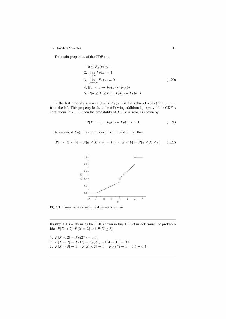
value in the interval (−∞, x]. Figure 1.3 depicts the exemplifying CDF
FX (x) =
0, x < −1x+110
, −1 ≤ x < 2x5, 3 ≤ x < 4
1, x ≥ 4
. (1.19)
1.5 Random Variables 11
The main properties of the CDF are:
1. 0 ≤ FX (x) ≤ 1
2. limx→∞
FX (x) = 1
3. limx→−∞
FX (x) = 0 (1.20)
4. If a ≤ b ⇒ FX (a) ≤ FX (b)
5. P[a ≤ X ≤ b] = FX (b) − FX (a−).
In the last property given in (1.20), FX (a−) is the value of FX (x) for x → a
from the left. This property leads to the following additional property: if the CDF is
continuous in x = b, then the probability of X = b is zero, as shown by:
P[X = b] = FX (b) − FX (b−) = 0. (1.21)
Moreover, if FX (x) is continuous in x = a and x = b, then
P[a < X < b] = P[a ≤ X < b] = P[a < X ≤ b] = P[a ≤ X ≤ b]. (1.22)
Fig. 1.3 Illustration of a cumulative distribution function
Example 1.3 – By using the CDF shown in Fig. 1.3, let us determine the probabil-
ities P[X < 2], P[X = 2] and P[X ≥ 3].
1. P[X < 2] = FX (2−) = 0.3.
2. P[X = 2] = FX (2) − FX (2−) = 0.4 − 0.3 = 0.1.
3. P[X ≥ 3] = 1 − P[X < 3] = 1 − FX (3−) = 1 − 0.6 = 0.4.

12 1 A Review of Probability and Stochastic Processes
1.5.2 Types of Random Variables
In this section we address the types of random variables and the corresponding
mathematical functions that characterize them.
1.5.2.1 Discrete Random Variables
A discrete random variable is the one that assumes discrete countable values. These
values can be in a finite or in an infinite range.
Discrete random variables are usually represented in terms of its probability mass
function (PMF), defined by
pX (x) , P[X = x], x real. (1.23)
The cumulative distribution function of a discrete random variable is the sum of
unit-step functions u(x) located at each value of X , and weighted by each of the
corresponding PMF values:
FX (x) =∑
k
pX (xk)u(x − xk). (1.24)
The magnitude of the “jumps” in the CDF at x = xk is the value of P[X = xk].
1.5.2.2 Continuous Random Variables
A continuous random variable has a continuous cumulative distribution function
for all of its values. In other words, a continuous random variable is the one that
assumes continuous values in a finite or in an infinite range. According to (1.21),
the probability of occurrence of a particular value for a continuous random variable
is zero, that is, P[X = x] = 0, for any value of x .
Continuous random variables are usually characterized by a probability density
function (PDF), defined as the first derivative of the CDF, as shown by:
fX (x) ,d FX (x)
dx. (1.25)
The PDF is called a probability density in the sense that it represents the proba-
bility of X be in a small interval in the neighborhood of x . More details about the
PDF will be given later.
1.5.2.3 Mixed Random Variables
As the name suggests, mixed random variables are those represented by cumulative
distribution functions having continuous and discontinuous portions. An example of
such CDF was given in Fig. 1.3.

1.5 Random Variables 13
For mixed random variables the CDF can be written in terms of discrete and
continuous parts, as shown below for one discrete component and one continuous
component, that is,
FX (x) = pFX1(x) + (1 − p)FX2(x), (1.26)
where p is the probability of occurrence of the discrete event, FX1(x) is the CDF of
the discrete component random variable and FX2(x) is the CDF of the continuous
component random variable.
1.5.2.4 Probability Density Function of a Discrete Random Variable
The cumulative distribution function of a discrete random variable can be written in
terms of the Dirac delta function δ(z) as [9, p. 151]
FX (x) =∫ x
−∞
∑
k
pX (xk)δ(z − xk)dz, (1.27)
which suggests that the probability density function of a discrete random variable is
given by
fX (x) =d FX (x)
dx=
∑
k
pX (xk)δ(x − xk). (1.28)
We can notice the slight difference between this probability density function and
the probability mass function defined in (1.23). Graphically, the representation of
the PDF can be used for representing a PMF. However, the PDF is mathematically
more adequate from the point of view of its relation with the CDF.
1.5.2.5 Properties of the Probability Density Function
The probability density function has the following main properties:
1. fX (x) ≥ 0
2. P[a ≤ X ≤ b] =∫ b
a
fX (x)dx
3. FX (x) =∫ x
−∞fX (t)dt
4.
∫ +∞
−∞fX (t)dt = 1.
(1.29)
The second, third and fourth properties in (1.29), when applied to a discrete ran-
dom variable, will lead to equivalent results produced by the following operations
involving the probability mass function:

14 1 A Review of Probability and Stochastic Processes
1. P[B] =∑
x∈B
pX (x)
2. FX (x) =∑
k
pX (xk)u(x − xk) (1.30)
3.∑
x∈S
pX (x) = 1.
1.5.2.6 The Normalized Histogram as an Approximation for the PDF
From [4, p. 348], a histogram is “a graph of vertical bars representing a frequency
distribution in which the groups or classes of items are marked on the x-axis, and
the number of items in each class is indicated by a horizontal line segment drawn
above the x-axis at a height equal to the number of items in the class”.
Example 1.4 – This example aims at clarifying the above definition. Suppose you
have collected the height of 100 graduate students, obtaining the following values
in meters:
1.62 1.74 1.54 1.93 1.71 1.70 1.71 1.61 1.53 1.63
1.65 1.74 1.64 1.76 1.69 1.63 1.76 1.66 1.60 1.77
1.70 1.71 1.77 1.63 1.73 1.70 1.61 1.58 1.60 1.72
1.62 1.72 1.67 1.73 1.64 1.59 1.77 1.68 1.74 1.78
1.51 1.78 1.71 1.49 1.73 1.77 1.68 1.76 1.75 1.81
1.77 1.74 1.68 1.67 1.63 1.73 1.80 1.82 1.82 1.87
1.56 1.80 1.75 1.61 1.74 1.73 1.51 1.69 1.77 1.73
1.86 1.81 1.80 1.67 1.73 1.78 1.92 1.81 1.77 1.64
1.55 1.80 1.64 1.50 1.63 1.55 1.60 1.68 1.96 1.73
1.73 1.61 1.88 1.72 1.62 1.82 1.67 1.54 1.65 1.56
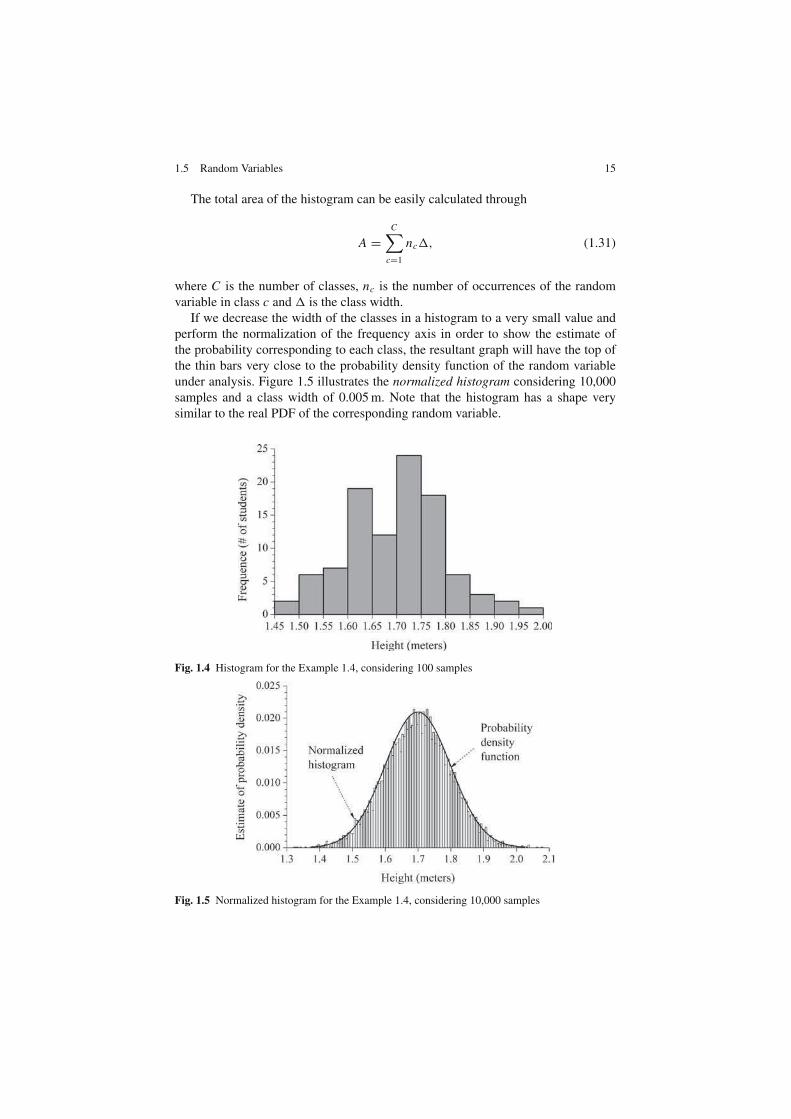
Following the definition above, you will obtain the histogram shown in Fig. 1.4.
In this histogram, the range of heights was divided into 11 classes or bins. In the ver-
tical axis are shown the number of students having their height in the corresponding
class in the horizontal axis. For example, there are 6 students with heights between
1.50 and 1.55 m.
The information that there are 6 students with heights between 1.50 and 1.55 m
can not be converted into an estimate of probability, unless, in the light of the relative
frequency definition for probability, we have an infinite number of samples. How-
ever, if this number is high enough, a good probability estimate can be obtained. For
example, if we had 10,000 samples in Example 1.4, the division of the number of
students having heights between 1.50 and 1.55 m by the total area of the histogram
would result in a good approximation of the probability of the student height be in
this range.
1.5 Random Variables 15
The total area of the histogram can be easily calculated through
A =C
∑
c=1
nc∆, (1.31)
where C is the number of classes, nc is the number of occurrences of the random
variable in class c and ∆ is the class width.
If we decrease the width of the classes in a histogram to a very small value and
perform the normalization of the frequency axis in order to show the estimate of
the probability corresponding to each class, the resultant graph will have the top of
the thin bars very close to the probability density function of the random variable
under analysis. Figure 1.5 illustrates the normalized histogram considering 10,000
samples and a class width of 0.005 m. Note that the histogram has a shape very
similar to the real PDF of the corresponding random variable.
Fig. 1.4 Histogram for the Example 1.4, considering 100 samples
Fig. 1.5 Normalized histogram for the Example 1.4, considering 10,000 samples
16 1 A Review of Probability and Stochastic Processes
In summary, the histogram is a very useful tool for estimating the shape of the
probability density function of a random variable. The greater the sample size, the
better the approximation between the normalized histogram and the PDF will be.
The smaller the class width, the greater the histogram ability of recording short-term
undulations in the estimated PDF will be. This is particularly useful in the case of
multimodal PDFs, i.e. PDFs that exhibit two or more “peaks”.
1.6 Conditional Probability Densities and Mass Functions
In (1.13) we presented the definition of the conditional probability and, from this
definition, in (1.14) and (1.16) we derived the Bayes rule and the total probability
theorem, respectively. Now we are able to extend those concepts to conditional den-
sities and mass functions. The concepts we are about to present in this section are
of great relevance, since in practice we commonly encounter random variables that
are not independent from each other.
We start by defining the conditional probability mass function for discrete ran-
dom variables X and Y . The conditional PMF of X , given Y = y is given by
pX (x |y) = P[X = x |Y = y] =P[X = x, Y = y]
P[Y = y]=
pX,Y (x, y)
pY (y). (1.32)
If X and Y are continuous random variables we have the following conditional
PDF of X , given Y = y:
fX (x |y) =fX,Y (x, y)
fY (y)=
fY (y|x) fX (x)
fY (y). (1.33)
1.6.1 The Bayes Rule Revisited
Suppose that we are interested in knowing the a posteriori probability of an event
B, given X = x has occurred, P[B|X = x], from the knowledge of the conditional
probability density function of x given B, fX (x |B), from the a priori probability of
B, P[B], and from the total probability density fX (x). The Bayes rule for probabil-
ity density functions states that [15, p. 84]
P[B|X = x] =fX (x |B)P[B]
fX (x), fX (x) 6= 0. (1.34)
This is an important result, largely used in parameter estimation based on the
maximum a posteriori (MAP) probability criterion. In Chaps. 4 and 5 we apply this
version of Bayes rule for developing two important decision rules used in digital
communication systems: the MAP itself and the maximum likelihood (ML).
1.7 Statistical Averages of Random Variables 17
1.6.2 The Total Probability Theorem Revisited
Multiplying both sides of (1.34) by fX (x) and integrating the result we obtain
P[B] =∫ ∞
−∞P[B|X = x] fX (x)dx . (1.35)
This is also an important result and represents the continuous version of the total
probability theorem given in (1.16). It states that if we know the probability of
occurrence of an event, given the value of another random variable, the “average”
probability of the event is obtained by averaging the conditional probability over all
possible values of the random variable to which the probability is conditioned.
Although the definition of the total probability theorem given in (1.16) applies
directly to discrete random variables, it is worth rewriting it in terms of the PMF of
the condition discrete random variable, as follows:
P[B] =∑
k
P[B|X = xk]pX (xk). (1.36)
1.7 Statistical Averages of Random Variables
As pointed out at the beginning of this chapter, though random phenomena can not
be precisely predicted, they exhibit regularities that permit some sort of inference
and a given confidence on such inference. These regularities are given by statistical
averages in a more formal and more generic sense that the intuitive concept about
averages that we might have in mind.
An statistical average of a random variable or random process is usually denoted
by the expectation or expected value operator E[·].
1.7.1 Mean of Random Variables
One of the most important statistical averages is the mean. For a discrete random
variable X , the mean is given by
E[X ] = µX =∑
k
xk pX (xk), (1.37)
where xk are the possible values assumed by the random variable and pX (xk) is
the value of the probability mass function for X = xk . The shorthand notation µX
is sometimes preferred for the sake of notational simplicity.
18 1 A Review of Probability and Stochastic Processes
For a continuous random variable X , the mean is given by
E[X ] = µX =∫ ∞
−∞x fX (x)dx, (1.38)
where fX (x) is the probability density function of X .
If a random variable is defined in terms of another random variable, say, Y =g(X ), then the mean value of Y is given by
E[Y ] =∑
k
g(xk)pX (xk), (1.39)
if the random variables are discrete, and
E[Y ] =∫ ∞
−∞y fY (y)dy =
∫ ∞
−∞g(x) fX (x)dx, (1.40)
if the random variables are continuous.
The concept of mean can be extended to the case in which a random variable Y
is written in terms of multiple random variables, that is, Y = g(X1, X2, . . . , Xn).
For example, for multiple continuous random variables we have:
E[Y ] =∫ ∞
−∞· · ·
∫ ∞
−∞g(x1, x2, . . . , xn) fX1...Xn
(x1, x2, . . . , xn)dx1dx2 . . . dxn .
(1.41)
The mean of the sum of random variables is the sum of the individual means:
E
[
n∑
i=1
X i
]
=n
∑
i=1
E[X i ] (1.42)
In Sect. 1.4 we discussed the concept of a joint event end the concept of indepen-
dent events. We have seen that the joint probability of occurrence of independent
events is the product of the probabilities of the individual events. This concept
is analogous to the case of probability functions of random variables, that is, two
discrete random variables are said to be independent random variables if the joint
probability mass function is the product of the individual (marginal) probability
mass functions of the discrete random variables:
pX,Y (x j , yk) = pX (x j )pY (yk), (1.43)
for all j and k. Equivalently, two continuous random variables are said to be inde-
pendent if the joint probability density function is the product of the marginal prob-
ability density functions of the continuous random variables:
fX,Y (x, y) = fX (x) fY (y). (1.44)

1.7 Statistical Averages of Random Variables 19
The mean of the product between independent random variables is the product
of the individual means, that is,
E[XY ] = E[X ]E[Y ]. (1.45)
1.7.2 Moments of Random Variables
The n-th moment of a random variable X is defined as the expected value of the
n-th power of X , as shown below for a continuous random variable:
E[Xn] =∫ ∞
−∞xn fX (x)dx, (1.46)
from where we can notice that the first moment of a random variable corresponds to
its mean.
The second moment E[X2] of a random variable X is of great importance and is
usually referred to as the mean-square value of the random variable. We shall see at
the end of this chapter that the second moment of a random process corresponding
to a voltage waveform is the total average power of the waveform.
We also have the definition of the n-th central moment as the expected value of
the centralized random variable, where centralized indicates that the mean is taken
out of the computation of the moment, as shown by:
E[(X − µX )n] =∫ ∞
−∞(x − µX )n fX (x)dx . (1.47)
Similarly, for discrete random variables we have
E[(X − µX )n] =∑
k
(xk − µX )n pX (xk). (1.48)
Also of great importance is the second central moment, usually referred to as
the variance of the random variable. We shall see at the end of this chapter that the
second central moment of a random process corresponding to a voltage waveform is
the total AC power2 of the waveform. The shorthand notations for the variance of a
random variable X are usually var[X ] or σ2X , where σX is called standard deviation
or root-mean-square (rms) value of X .
If a is a constant, then we have the following main properties of the variance:
2 AC stands for alternating current. DC stands for direct current.

20 1 A Review of Probability and Stochastic Processes
1. If X = a, then var[X ] = 0
2. If Y = X + a, then var[Y ] = var[X ] (1.49)
3. If Y = aX, then var[Y ] = a2 var[X ].
From (1.38) and (1.47) we can write the important relation:
σ 2X = E[X2] − µ2
X . (1.50)
Again, we shall see at the end of this chapter that for a random process cor-
responding to a voltage waveform, (1.50) states that the average AC power σ 2X is
equal to the total average power E[X2] minus the average DC power E2[X ], which
is an intuitively satisfying interpretation.
The relation among the central moment, the non-centralized moment and the first
moment of a random variable can be generalized as follows [15, p. 193]:
E[(X − µX )n] =n
∑
k=0
(
n
k
)
(−1)kµkX E[Xn−k], (1.51)
where the binomial coefficient was defined in (1.11).
1.7.3 Joint Moments of Random Variables
The joint moment of two continuous random variables X and Y is defined by
E[X i Y n] =∫ ∞
−∞
∫ ∞
−∞x i yn fX,Y (x, y) dxdy. (1.52)
For discrete random variables we have
E[X i Y n] =∑
j
∑
k
x ij x
nk pX,Y (x j , yk), (1.53)
where the order of the joint moment is given by i + n.
Similarly, the joint central moment of two random variables X and Y is E[(X −µX )i (Y − µY )n]. For continuous random variables it is given by
E[(X − µX )i (Y − µY )n] =∫ ∞
−∞
∫ ∞
−∞(x − µX )i (y − µY )n fX,Y (x, y) dxdy. (1.54)
1.7 Statistical Averages of Random Variables 21
1.7.3.1 Correlation Between Random Variables
The second-order joint moment between two random variables is called correlation
and it is obtained with i = 1 and n = 1 in (1.52), resulting in the second-order
moment E[XY ].
Two random variables X and Y are said orthogonal if their correlation is zero.
If two orthogonal random variables are also independent, from (1.45) E[XY ] =E[X ]E[Y ] = 0, which means that E[X ], E[Y ], or both are zero.
1.7.3.2 Covariance Between Random Variables
The second-order joint central moment between two random variables is called
covariance and it is obtained with i = 1 and n = 1 in (1.54), yielding
cov[X, Y ] = E[(X − µX )(Y − µY )]
= E[XY ] − E[X ]E[Y ].(1.55)
Two random variables X and Y are said to be uncorrelated if their covariance
is zero. The degree of correlation is usually measured by a normalized covariance
ranging from −1 to 1 and called correlation coefficient, which is defined by
ρ ,cov[X, Y ]√
σ 2Xσ 2
Y
. (1.56)
Note that, with the condition (1.45) in (1.55), if two random variables are statis-
tically independent, they are also uncorrelated. However, although two uncorrelated
random variables satisfy E[XY ] = E[X ]E[Y ], they are also independent if and
only if their joint probability density or mass function is the product of the marginal
probability density or mass functions, according to (1.43) and (1.44).
Note also that if two random variables are orthogonal, then E[XY ] = 0. With
this condition in (1.55), these variables will be uncorrelated if and only if one of
their expected values, or both, are zero.
1.7.4 The Characteristic and the Moment-Generating Functions
The characteristic functions (CF) of continuous and discrete random variables are
defined by the statistical averages:
ψX ( jω) , E[e jωX ] =
∫ ∞−∞ e jωx fX (x)dx if X is continuous.
∑
k
e jωxk pX (xk) if X is discrete. (1.57)
Note that the characteristic function is similar to the Fourier transform (see
Chap. 2), except by the sign of the exponential. Then, the probability density

22 1 A Review of Probability and Stochastic Processes
function can be obtained from the characteristic function by means of the “inverse
Fourier transformation”, leading to
fX (x) =1
2π
∫ ∞
−∞e− jωxψX ( jω)dω. (1.58)
One of the major applications of the characteristic function is in the determina-
tion of the moments of a random variable. This is accomplished through the moment
theorem, which is given by
E[Xn] = (− j)n dnψX ( jω)
dωn
∣
∣
∣
∣
ω=0
. (1.59)
Another application of the characteristic function is the estimation of the proba-
bility density function of a random variable from experimental measurements of the
moments [15].
The probability generating function [9, p. 187] or moment-generating function
(MGF) [10, p. 114; 15, p. 211; 18, p. 248] of a random variable is defined anal-
ogously to the characteristic function and has essentially the same applications.
However, the characteristic function always exists, which is not the case of the
moment-generating function [1, pp. 194, 350].
The moment-generating functions of continuous and discrete random variables
are defined by
φX (s) , E[es X ] =
∫ ∞−∞ esx fX (x)dx if X is continuous.
∑
k
esxk pX (xk) if X is discrete. (1.60)
The MGF of a continuous random variable is similar to the Laplace transforma-
tion (see Chap. 2), the difference being that the MGF is defined for all s real. Then,
the MGF and PMF or PDF form a transform pair.
The moment theorem also applies in the case of the MGF and is given by
E[Xn] =dnφX (s)
dsn
∣
∣
∣
∣
s=0
. (1.61)
Other important properties of the moment-generating function are:
1. φX (s)|s=0 = 1
2. If Y = aX + b, then φX (s) = esbφX (as).(1.62)
In Sect. 1.10 we shall discuss other properties of the characteristic function that
are also applicable to the moment-generating function, in the context of the sum of
random variables. The summarized concepts considered up to this point suffice for
the continuity of the presentation.
1.8 Some Discrete Random Variables 23
1.7.5 Conditional Expected Value
The conditional expected value E[X |y] is the expected value of the random variable
X , given a value of another random variable Y be equal to y. Mathematically, if X
and Y are both continuous random variables,
E[X |y] = E[X |Y = y] =∫ ∞
−∞x fX (x |y)dx . (1.63)
If X and Y are both discrete random variables, the conditional expectation is
E[X |y j ] = E[X |Y = y j ] =∑
k
xk pX (xk |y j ). (1.64)
From the total expectation law, E[E[X |Y ]] = E[X ]. As a consequence, we have
the following unconditional expectations:
E[X ] =
∫ ∞−∞ E[X |y] fY (y)dy, if X and Y are continuous.
∑
j
E[X |y j ]pY (y j ), if X and Y are discrete. (1.65)
1.8 Some Discrete Random Variables
In what follows we present some discrete random variables, examples of their use,
their probability mass functions, main statistical averages and moment-generating
functions. We omit further details for the sake of brevity. For more information, the
interested reader is encouraged to consult the references listed at the end of the chap-
ter. A great number of details about several distributions can also be found online
at the Wikipedia encyclopedia [16] or at the Wolfram MathWorld [17]. Some of the
simulations considered in this chapter will also help clarifying and exemplifying the
concepts about these random variables.
1.8.1 Bernoulli Random Variable
This discrete random variable is largely used to model random phenomena that can
be characterized by two states. For example: on/off, head/tail, bit “0” / bit “1”. These
states are commonly associated to the terms success or failure. The attribution of
these terms to a given state is somewhat arbitrary and depends on what we want for
the meaning of the states in relation to the actual observed phenomenon.
A Bernoulli random variable can also be used to model any random phenomena
for which an indicator function IA is used to signalize the occurrence of an event
A. The indicator function will be a Bernoulli random variable that assumes the state
“1” (success) if the event under observation occurs and “0” (failure) otherwise. If

24 1 A Review of Probability and Stochastic Processes
p is the probability of success and q = (1 − p) is the probability of failure in this
Bernoulli trial, then p = P[A].
The probability mass function, mean, variance and moment-generating function
of a Bernoulli random variable X with parameter p are, respectively:
1. pX (x) =
p, x = 1
1 − p, x = 0
0, otherwise
2. E[X ] = p (1.66)
3. var[X ] = p(1 − p)
4. φX (s) = 1 − p + pes .
1.8.2 Binomial Random Variable
A binomial random variable X counts the number of successes in n Bernoulli trials
or, equivalently, X is the sum of n Bernoulli random variables. Its applications arise,
for example, in the analysis of the number of ones (or zeros) in a block of n bits at
the output of a binary source. If we assign the probability of success p of a Bernoulli
trial to the probability of bit errors in a digital communication system, the number
of bits in error in a block of n bits is a binomial random variable.
The probability mass function, mean, variance and moment-generating function
of a binomial random variable X with parameters n and p are, respectively:
1. pX (x) =(
n
x
)
px (1 − p)n−x
2. E[X ] = np (1.67)
3. var[X ] = np(1 − p)
4. φX (s) = (1 − p + pes)n.
1.8.3 Geometric Random Variable
The geometric random variable characterizes the number of failures before a success
or between successes in a sequence of Bernoulli trials. Alternatively, a geometric
random variable can characterize the number of Bernoulli trials needed to produce
one success, no matter if a success has or has not occurred before. In what follows
we consider the first case, for which the results are 0, 1, 2, . . ., etc.
As an example, if we assign the probability of success p of a Bernoulli trial to the
probability of bit errors in a digital communication system, the number of correct
bits before a bit error occurs is a geometric random variable.

1.8 Some Discrete Random Variables 25
The probability mass function, mean, variance and moment-generating function
of a geometric random variable X with parameter p are, respectively:
1. pX (x) =
p(1 − p)x , x = 0, 1, 2, . . .
0, otherwise
2. E[X ] =1 − p
p
3. var[X ] =1 − p
p2
4. φX (s) =p
1 − (1 − p)es.
(1.68)
The geometric random variable is the only discrete memoryless random variable.
This means that if you are about to repeat a Bernoulli trial, given that the first suc-
cess has not yet occurred, the number of additional trials until a success shows up
does not depend on how many failures have been observed till that moment. As an
example, the die or the coin you throw in a given instant is not influenced by the
failures or successes up to that instant.
1.8.4 Poisson Random Variable
A Poisson random variable is used to characterize the number of occurrences of a
random, normally rare event in a given observation interval or space. Here the term
“rare” is determined according to the observation interval or space. In other words,
the event will occur a few times, on average, in the observed time or space.
If we define α as the average number of occurrences of the event in a specific
observation interval or space, λ = 1/α can be regarded as the average rate of occur-
rence of the Poisson event.
The probability mass function, mean, variance and moment-generating function
of a Poisson random variable X with parameter α are, respectively:
1. pX (x) =
αx e−α
x!, α > 0, x = 0, 1, 2, . . .
0, otherwise
2. E[X ] = α (1.69)
3. var[X ] = α
4. φX (s) = eα(es−1).
A binomial distribution with large n and small p can be approximated by a Pois-
son distribution with parameter α = np, according to
pX (x) =(
n
x
)
px (1 − p)n−x ∼=npx
x!e−np. (1.70)

26 1 A Review of Probability and Stochastic Processes
Simulation 1.2 – Discrete Random Variables
File – CD drive:\Simulations\Probability\Discrete RV.vsm
Default simulation settings: Frequency = 1 Hz; End = 10,000
seconds. Probability of success for the configurable Bernoulli sources:
p = 0.5.
This experiment aims at helping the reader to understand some concepts related to
discrete random variables. All discrete random variables considered in this section
are generated: Bernoulli, binomial, Poisson and geometric. The variance and mean
are estimated for each random variable. VisSim/Comm has a specific block to do
these estimates, but in fact these blocks use sample averages, a topic covered later
on in this chapter.
In what follows we shall analyze each of the above random variables. The
Bernoulli source generates a random sequence of zeros and ones during the sim-
ulation interval. The probability of success of the Bernoulli trial is represented here
by the probability of generating a binary “1”. Using the default simulation settings,
run the experiment and observe the values of the mean and variance of the Bernoulli
random variable. According to (1.66), these values should be E[X ] = p = 0.5
and var[X ] = p(1 − p) = 0.25. Look inside the block “histograms” and rerun
the simulation. Observe that, for p = 0.5, in fact the frequencies of occurrence of
ones and zeroes are roughly the same. Change the value of p and compare again
the variance and mean of the Bernoulli random variable with the theoretical results.
Analyze the histogram and observe the dependence of its shape on the value of p.
Still considering the first part of the experiment, now let us shift our attention to
the binomial random variable. Observe that, according to the theoretical definition, it
has been generated as the sum of n = 10 Bernoulli random variables. The simulation
does this by summing-up 10 consecutive Bernoulli results. The updating of the sum
is made by entering a new Bernoulli value to be added and discarding the tenth
one. Run the simulation and observe the mean and variance of the binomial random
variable. According to (1.67), E[X ] = np = 5 and var[X ] = np(1 − p) = 2.5.
Observe the histogram and, with the help of (1.67), determine the PMF and compare
its shape with the shape of the histogram. Change the value of p as you wish and
repeat the calculations.
The second part of the experiment generates a geometric random variable and
repeats in a different way the generation of a binomial random variable: now, the
number of successes in each 10 Bernoulli trials is being counted, generating a bino-
mial random variable.
According to the theory, the number of failures before each success of a Bernoulli
trial has a geometric distribution. The number of failures before the first success is
also a geometric random variable. Note that the number of failures before each suc-
cess is updated several times during the simulation and that the number of failures
before the first success is updated only in a simulation run basis.
Using the default settings, run the simulation and observe the mean and the vari-
ance of the geometric random variable. Compare the results with those obtained via

1.9 Some Continuous Random Variables 27
(1.68). Observe also the shape of the histogram, which corresponds to the shape of
the probability mass function of the geometric distribution.
The third and last part of the experiment generates a Poisson random variable.
Since a Poisson event occurs rarely, the corresponding random variable was gen-
erated by a binomial source with p = 0.002 and n = 1,000. According to the
theory, a binomial random variable with such a small p and large n approximates a
Poisson random variable. Using the default simulation settings, run the simulation
and observe the “event display”. Note that, in fact, a Poisson event is relatively
rare. You should observe something varying around 10np = 20 Poisson events at
the output of the “accumulated successes” block, where the multiplier 10 is the
number of observation intervals of 1,000 seconds during the overall simulation time
of 10,000 seconds.
Since the Poisson event is relatively rare, to have a better estimate of the random
variable statistics, we must increase the simulation time to, say, 1,000,000 seconds.
Run the simulation and observe the “accumulated successes”. Divide this number
by the observation time of 1,000 seconds. You will find a value very close to 2, the
actual mean of the Poisson random variable. Compare this value of mean and the
variance with the expected theoretical results given by (1.69), where α = np =1, 000 × 0.002 = 2 is the expected number of events in 1,000 seconds, which by
its turn is the mean and the variance of the Poisson random variable. Observe also
the shape of the histogram, which corresponds to the shape of the probability mass
function of the Poisson distribution.
Explore inside the individual blocks. Try to understand how they were imple-
mented. Create and investigate for yourself new situations and configurations of the
simulation parameters and try to reach your own conclusions.
1.9 Some Continuous Random Variables
In this section we present some continuous random variables, examples of their use,
their probability density functions, main statistical averages and moment-generating
functions. Since this is a review chapter, we omit further information for the sake
of brevity. Details about several continuous distributions can also be found online
at the Wikipedia encyclopedia homepage [16] or in the Wolfram MathWorld home-
page [17]. Some of the simulations addressed throughout this chapter will also help
clarifying and exemplifying the concepts about the continuous random variables
considered here.
1.9.1 Uniform Random Variable
As the name suggests, a uniform random variable has its probability density func-
tion uniformly distributed in a given range. The probability density function, mean,
variance and moment-generating function of a uniform random variable X with
parameters a and b are, respectively:
28 1 A Review of Probability and Stochastic Processes
1. fX (x) =
1b−a
, a ≤ x ≤ b
0, otherwise
2. E[X ] =a + b
2
3. var[X ] =(b − a)2
12
4. φX (s) =ebs − eas
s(b − a).
(1.71)
Many physical phenomena are characterized by a uniform distribution. For exam-
ple, the uniform quantization used as part of the digitalizing process of a signal
generates an error that is uniformly distributed around zero. Moreover, when deal-
ing with random number generation, a uniform random variable is the basis for the
generation of random variables having other distributions. This last application will
become clearer later on in this chapter, where the generation of random numbers is
covered.
1.9.2 Exponential Random Variable
The probability density function, mean, variance and moment-generating function
of an exponential random variable X with parameter λ are, respectively:
1. fX (x) =
λe−λx , x ≥ 0
0, otherwise
2. E[X ] =1
λ
3. var[X ] =1
λ2
4. φX (s) =λ
λ − s.
(1.72)
The parameter λ is usually referred to as the rate parameter. The exponential
distribution can be seen as the continuous counterpart of the geometric distribution
and, as such, is the only continuous memoryless random variable. In terms of the
conditional probability, this means that
P[X > x1 + x2|X > x1] = P[X > x2], x1 and x2 ≥ 0. (1.73)
The exponential random variable has many applications and, among them we can
mention: the time until the occurrence of the first event and between the events in
1.9 Some Continuous Random Variables 29
a Poisson random variable is exponentially-distributed. In this case, if the Poisson
has α as the average number of occurrences of the events in a specific observation
interval To, λ = α/To is the average rate of occurrence of the Poisson events. The
exponential distribution can also be used to characterize the time between beeps in
a Geiger counter, the time between telephone calls or how long it takes for a teller
to serve a client.
1.9.3 Gaussian Random Variable
The probability density function, mean, variance and moment-generating function
of a Gaussian random variable X with mean µ and standard deviation σ are, respec-
tively:
1. fX (x) =1
σ√
2πe−(x−µ)2/2σ 2
2. E[X ] = µ
3. var[X ] = σ 2
4. φX (s) = esµ+s2σ 2/2.
(1.74)
The Gaussian random variable has a major importance for the study of several
areas, particularly for the study of digital transmission. It is used, for example, to
model thermal noise generated by the random motion of electrons in a conductor.
This noise is the omnipresent impairment whose influence must be considered in
the design of any communication system. Moreover, a Gaussian distribution is used
to characterize the sum of independent random variables having any distribution.
The central limit theorem, a subject treated later on in this chapter, states that under
a variety of conditions the PDF of the sum of n independent random variables con-
verges to a Gaussian PDF for a sufficient large n.
Due to its importance for the study of communication systems, in what follows
we shall devote a little bit more attention to the Gaussian random variable.
One of the problems that often arise in practice is related to the computation of
the area under a Gaussian PDF. This computation is usually related to the estimate
of probabilities of rare events, which are normally associated to the area of the tails
of a Gaussian distribution. To elaborate more on this matter, consider the problem
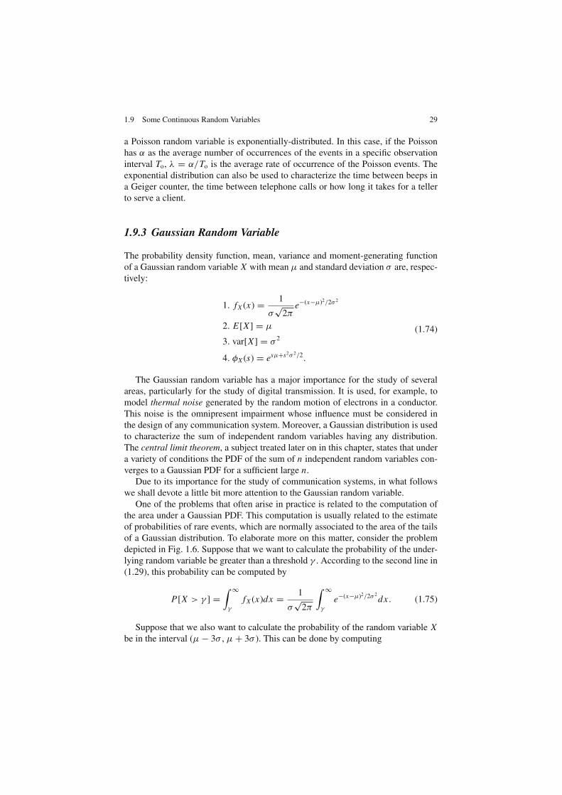
depicted in Fig. 1.6. Suppose that we want to calculate the probability of the under-
lying random variable be greater than a threshold γ . According to the second line in
(1.29), this probability can be computed by
P[X > γ ] =∫ ∞
γ
fX (x)dx =1
σ√
2π
∫ ∞
γ
e−(x−µ)2/2σ 2
dx . (1.75)
Suppose that we also want to calculate the probability of the random variable X
be in the interval (µ − 3σ , µ + 3σ ). This can be done by computing
30 1 A Review of Probability and Stochastic Processes
P[(µ − 3σ ) < X < (µ + 3σ )] = 1 −2
σ√
2π
∫ ∞
µ+3σ
e−(x−µ)2/2σ 2
dx . (1.76)
When computing probabilities like in (1.75) and (1.76), it is usual to operate
alternatively with the so-called normalized Gaussian random variable, which has
µ = 0 and σ = 1. This random variable is often referred to as a N (0, 1) or normal
random variable. The reason is that we become able to compute probabilities from
Gaussian random variables with any mean and any standard deviation from a single
normal density. Moreover, areas under the N (0, 1) density function are tabulated in
several references, facilitating even more our work. As an example, the probability
in (1.75) can be computed from the normal Gaussian PDF according to
P[X > γ ] =1
√2π
∫ ∞
γ−µ
σ
e−x2/2dx . (1.77)
Fig. 1.6 Normalized Gaussian PDF and some probabilities obtained from it
The probability in (1.76) can be computed analogously.
Unfortunately, none of the preceding three integrals has a closed-form analyti-
cal solution and we must resort to numerical integration to solve them. The usual
numerical solution makes use of the complementary error function or some of its
variants (see Appendix A.2). The complementary error function is defined by
erfc(u) ,2
√π
∫ ∞
u
exp[
−z2]
dz. (1.78)
It is apparent from (1.78) that erfc(u) computes two times the area on the right
of u, under a Gaussian PDF of zero mean and variance 1/2. It is then useful for the
purpose of determining areas under a Gaussian PDF.

1.9 Some Continuous Random Variables 31
Applying (1.78) to the probability in (1.75) we have a very useful expression:
P[X > γ ] =1
2erfc
(
γ − µ
σ√
2
)
, (1.79)
from where it follows that the probability in (1.76) can be determined by
P[(µ − 3σ ) < X < (µ + 3σ )] = 1 − erfc
(
3√
2
)
∼= 0.9973. (1.80)
This interesting result shows that 99.73% of the area under a Gaussian PDF is
within the range (µ − 3σ , µ + 3σ ). For many practical purposes, these limits are
considered the limits of excursion of the underlying Gaussian random variable.
The computation of the complementary error function is a feature of many math-
ematics software tools like Mathcad, Matlab and Mathematica,3 of spreadsheet soft-
ware tools like Excel, or even in modern scientific calculators. The error function
or the complementary error function is also often tabulated in books on probability,
statistics and random processes and digital communications. Appendix A.2 provides
such a table.
1.9.4 Rayleigh Random Variable
The probability density function, mean, variance, mean square value and moment-
generating function of a Rayleigh random variable X with parameter Ω = 2σ 2 are,
respectively:
1. fX (x) =
2xΩ
e−x2
Ω , x ≥ 0
0, otherwise
2. E[X ] = σ
√
π
2
3. var[X ] =4 − π
2σ 2 (1.81)
4. E[X2] = 2σ 2 = Ω
5. φX (s) = 1 + σ seσ 2s2/2
√
π
2
[
erf
(
σ s√
2
)
+ 1
]
.
The Rayleigh random variable arises, for example, in complex Gaussian random
variables whose real and imaginary parts are independent and identically distributed
(i.i.d.) Gaussian random variables. In these cases the modulus of the complex Gaus-
sian random variable is Rayleigh-distributed.
3 Mathcad, Matlab, Mathematica and Excel are trademarks of Mathsoft, Inc., Mathworks, Inc.,Wolfram Research, Inc. and Microsoft Corporation, respectively.

32 1 A Review of Probability and Stochastic Processes
As we shall see in Chap. 3, the Rayleigh distribution is often used to characterize
the multipath fading phenomena in mobile communication channels.
Simulation 1.3 – Continuous Random Variables
File – CD drive:\Simulations\Probability\Continuous RV.vsm
Default simulation settings: Frequency = 100 Hz; End = 100 seconds.
Mean = 0 and standard deviation = 1 for the thermal (Gaussian) noise
source.
Complementary to the previous simulation, this experiment aims at helping the
reader to understand some concepts related to the continuous random variables:
uniform, Laplace, exponential, Gaussian and Rayleigh.
The first part of the experiment generates a uniform random variable from the
quantization error of a voice signal. The quantization process approximates the pos-
sibly infinite number of values of the input to a finite number of quantized levels. In
this experiment we are simulating a 10-bit uniform quantizer which represents the
input waveform by 210 = 1, 204 levels with a step-size q = 0.0156 volts, resulting
in a total dynamic range of approximately 16 volts.
The quantization error, defined as the subtraction of the quantized signal from
the un-quantized signal, has a uniform distribution with parameters, a = −q/2 =−0.0078 V and b = +q/2 = +0.0078 V. Run the simulation and observe the val-
ues of the mean and the variance of the uniform quantization error. Compare them
with the theoretical values obtained from (1.71). Observe also the corresponding
histogram and its similarity with the brick-wall shape of the theoretical PDF.
The voice signal excerpt used in this experiment has an approximate Laplace
distribution, which has probability density function, mean, variance and moment-
generating function given respectively by:
1. fX (x) =1
2re−|x−µ|/r , r > 0
2. E[X ] = µ
3. var[X ] = 2r2
4. φX (s) =eµs
1 − r2s2, |s| <
1
r.
(1.82)
In this simulation, the scale parameter r ∼= 1.43 and the mean µ = 0. The
variance of X is then var[X ] ∼= 4.09. Compare these results with those obtained in
the simulation. Observe also the histogram of the voice signal and compare to the
shape of the Laplace PDF obtained from (1.82).
Now go to the diagram in the second part of the experiment, which aims at ana-
lyzing the exponential random variable. You probably may have noticed the similar-
ity between this diagram and the one used for analyzing the Poisson random variable
in Simulation 1.2. In fact this is not a coincidence, since the time interval between

1.9 Some Continuous Random Variables 33
Poisson events or the time till the first Poisson event is an exponentially-distributed
random variable. The Poisson source was implemented in the same way as in Sim-
ulation 1.2, that is, from a binomial source with p = 0.002 and n = 1, 000. Note,
however, that the observation interval now is To = 10 s and that the binomial source
was derived from 100 Bernoulli trials per second, totalizing 1,000 trials in 10 s.
Again, the mean and the variance of the Poisson random variable are α = np = 2
and you will observe something varying around 10α = 20 Poisson events in the
“accumulated successes”, where 10 is the number of observation intervals of 10
seconds during the overall simulation time of 100 seconds.
The rate parameter of the exponential random variable is λ = α/To = 2/10 =0.2. Then, the mean of this random variable is 1/λ = 5 and its variance is 1/λ2 =25.
Increase the simulation “end time” to 10,000 seconds and run the simulation.
Compare the estimated mean and variance with the values just calculated. Now,
while rerunning the simulation, look inside the block “histograms”. Compare the
shape of the histograms with the theoretical Poisson PMF, determined via (1.69),
and the exponential PDF, determined via (1.72). Finally, divide the “accumulated
successes” by the total simulation time. You will find something around 0.2, which
is indeed the rate parameter λ.
Let us move to the third part of the experiment, where a Gaussian random vari-
able is generated and analyzed. The Gaussian source is simulating the thermal noise
commonly present in the analysis of communication systems. For the sake of com-
pleteness, both mean and standard deviation of the Gaussian random variable can be
configured. Using the default simulation settings, run the simulation and observe the
estimated values of the mean and variance. Compare them with those determined by
the Gaussian source configuration. While looking inside the block “histogram”, run
the simulation and observe the similarity between the shape of the histogram and
the bell-shaped Gaussian probability density function.
Note also that a block named “P[X > u]” has a default value of 2 as its u input.
According to (1.79), P[X > 2] = 0.023, a value that is estimated approximately in
the simulation by using the relative frequency definition for the probability (analyze
the construction of the block “P[X > u]”). Just to stress this concept, change the
mean and the standard deviation of the Gaussian source to 1 and 2, respectively.
Now, according to (1.79), P[X > 2] = 0.309. Compare this result with the one
obtained via simulation. Use a larger simulation “end time” if more accurate esti-
mates are desired.
Finally, the last part of the experiment generates and analyzes a Rayleigh random
variable. We shall see later on in this chapter that it is possible to determine the
probability density function of a random variable defined as a function of one or
more random variables. In this simulation, a Rayleigh random variable is generated
as follows: let X and Y be two independent Gaussian random variables with zero
mean and standard deviation σ . Define a new random variable R such that
R =√
X2 + Y 2. (1.83)

34 1 A Review of Probability and Stochastic Processes
This new random variable R is Rayleigh distributed. Moreover, let us define
another random variable Θ such that
Θ = arctan
(
Y
X
)
. (1.84)
The random variable Θ is uniformly-distributed between −π and +π .
The Gaussian sources in this part of the experiment have zero mean and standard
deviation σ =√
2/2. Then, according to (1.81), the Rayleigh random variable will
have E[R] ∼= 0.886, var[R] ∼= 0.215 and E[R2] = Ω = 2σ 2 = 1. The uniform
random variable will have zero mean and variance q2/12 = (2π )2/12 ∼= 3.29.
Compare these results with those produced by the simulation. Additionally, have a
look at the histograms of the random variables generated and compare them to the
probability density functions obtained from (1.71), for the uniform random variable,
and from (1.81) for the Rayleigh random variable.
Explore inside the individual blocks. Try to understand how they were imple-
mented. Create and investigate for yourself new situations and configurations of the
simulation parameters and try to reach your own conclusions.
1.9.5 Multivariate Gaussian Random Variables
Among the many multivariate distributions, the multivariate Gaussian distribution
arises in several practical situations. This is the reason for presenting a brief discus-
sion on this distribution in what follows.
Let X1, X2, . . ., X i , . . ., Xn be a set of Gaussian random variables with means
µi , variances σ 2i and covariances Ki j = cov[X i , X j ], i = 1, 2, . . ., n and j = 1, 2,
. . ., n. The joint PDF of the Gaussian random variables X i is given by
fX1,X2...Xn(x1, x2, . . . , xn) =
exp[
− 12(x − µX )TM−1(x − µX )
]
(2π )n/2(det M)1/2, (1.85)
where M is the n × n covariance matrix with elements Ki j , X is the n × 1 vector of
random variables, µX is the n ×1 vector of means, T denotes a matrix transposition,
M−1 is the inverse of the matrix M and det(M) is the determinant of M.
For the special case of a bivariate or two-dimensional Gaussian random variable
we have the following joint probability density function:
fX1,X2(x1, x2) =
exp
[
−σ 2
1 (x2 − µ2)2 + σ 22 (x1 − µ1)2 − 2ρσ1σ2(x1 − µ1)(x2 − µ2)
2σ 21 σ 2
2 (1 − ρ2)
]
2πσ1σ2
√
1 − ρ2,
(1.86)
where ρ is the correlation coefficient between X1 and X2, given by

1.10 Sum of Random Variables and the Central Limit Theorem 35
ρ =K12
σ1σ2
. (1.87)
Note from (1.86) that if two Gaussian random variables are uncorrelated, their
correlation coefficient is zero and, as a consequence, their joint probability density
function will be given by the product of the individual densities. Then, these two
variables are also statistically independent. In fact, this condition applies to any
set of Gaussian random variables, i.e. if Gaussian random variables are pair-wise
uncorrelated, they are also independent and their joint probability density function
is the product of the densities of the individual random variables in the set.
1.10 Sum of Random Variables and the Central Limit Theorem
Many problems encountered in the study of digital transmission are related to the
combination of random phenomena, which commonly appear as the sum of random
variables and random processes. In this section we review some of the main concepts
related to the sum of random variables, leaving for later the analysis of random pro-
cesses. Also in this section we present the central limit theorem, also in the context
of the sum of random variables. This important theorem has applications in several
areas and appears frequently in problems related to communication systems.
1.10.1 Mean and Variance for the Sum of Random Variables
Initially, let us define the random variable Y corresponding to the sum of n random
variables:
Y =n
∑
i=1
X i . (1.88)
The expected value of this sum is the sum of the expected values, that is,
E[Y ] =n
∑
i=1
E[X i ]. (1.89)
The variance of the sum is given by
var[Y ] =n
∑
i=1
var[X i ] + 2
n−1∑
i=1
n∑
j=i+1
cov[X i , X j ]. (1.90)
If the random variables are independent, from (1.55) cov[X i , X j ] = 0 for i 6= j .
Then, the variance of the sum is the sum of the variances:

36 1 A Review of Probability and Stochastic Processes
var[Y ] =n
∑
i=1
var[X i ]. (1.91)
1.10.2 Moments of the Sum of Random Variables
The characteristic function and the moment-generating function were defined in
Sect. 1.7.4. The moment theorem defined in that point is also useful in the case of
the sum of random variables, as we shall see below.
If the random variables X i are independent, the characteristic function of the
sum defined in (1.88) is given by
ψY ( jω) =∏
i
ψX i( jω). (1.92)
Moreover, if the random variables have the same distribution we say that they are
i.i.d. (independent and identically distributed). In this case we have
ψY ( jω) = [ψX ( jω)]n. (1.93)
Then, by applying the moment theorem given by (1.59), the n-th moment of the
sum of random variables can be determined.
1.10.3 PDF of the Sum of Random Variables
Let the random variable Y = X1 + X2. Its probability density function is given by
fY (y) =∫ ∞
−∞fX1 X2
(x1, y − x1)dx1 =∫ ∞
−∞fX1 X2
(y − x2, x2)dx2. (1.94)
If X1 and X2 are independent, the PDF of Y is
fY (y) =∫ ∞
−∞fX1
(y − x2) fX2(x2)dx2 =
∫ ∞
−∞fX1
(x1) fX2(y − x1)dx1, (1.95)
which means that the PDF of the sum of random variables is the convolution of the
individual PDFs. In general, the probability density function of the sum of indepen-
dent random variables is the convolution among the individual densities. However,
the computation of the resultant PDF can represent a hard and sometimes intractable
mathematical task. This problem can be overcome by applying (1.92) or (1.93) and
then the inverse transformation of the characteristic function according to (1.58).

1.10 Sum of Random Variables and the Central Limit Theorem 37
1.10.4 The Central Limit Theorem
The central limit theorem assumes several definitions and can be proved in several
different ways. One of its forms can be stated as follows: let X1, X2, . . ., X i , . . .,
Xn be a set of independent random variables, each of them having any probability
distribution, mean µi and variance σ 2i . The normalized random variable
Z =∑n
i=1 X i −∑n
i=1 µi√
∑ni=1 σ 2
i
(1.96)
has, in the limit of n → ∞, a Normal N (0, 1) cumulative distribution function. If
the random variables X i have the same mean µX and the same variance σ 2X , the
random variable
Z =1
n
∑n
i=1X i (1.97)
will be Gaussian in the limit, with mean µZ = µX and variance σ 2Z = σ 2
X/n.
In other words, if we sum-up n random variables, no matter their individual dis-
tributions, the resultant random variable approximates a Gaussian random variable
as n is increased.
One of the most widely uses of the central limit theorem is referred to as the
Gaussian approximation for the binomial distribution. We know from previous sec-
tions that a binomial random variable with parameters p and n is the sum of n
Bernoulli random variables having probability of success p. The resultant probabil-
ity mass function, mean and variance are, respectively:
1. pX (x) =(
n
x
)
px (1 − p)n−x
2. E[X ] = np
3. var[X ] = np(1 − p)
(1.98)
From the central limit theorem, for a large n the PMF above approximates a
Gaussian density with mean np and variance np(1 − p):
pX (x) ∼=1
√2πnp(1 − p)
exp
[
−(x − np)2
2np(1 − p)
]
. (1.99)
Figure 1.7 illustrates the Gaussian approximation for the binomial distribution,
considering n = 1, 000 and p = 0.8. Note that the asymmetry observed in the
binomial distribution for p 6= 0.5 tend to become practically invisible for a large n.
The central limit theorem has several applications in the design and analysis of
digital transmission systems. One of these applications will be illustrated with the
help of an example at the end of the next section.

38 1 A Review of Probability and Stochastic Processes
Fig. 1.7 Gaussian approximation for the binomial distribution (n = 1,000 and p = 0.8)
1.11 Transformations of Random Variables
A problem that frequently arises in practice is to find the probability density function
of a random variable Y = g(X ), knowing the PDF of X and the mapping rule from
one variable into another. Assuming that one value of X produces just one value of
Y , the PDF of Y is given by
fY (y) =fX (x)
|g′(x)|
∣
∣
∣
∣
x=g−1(y)
, (1.100)
where the inverse function g−1(y) is simply the value of x written in terms of y.
For the cases where the mapping function g(X ) is such that one value of X
produces more than one value of Y , firstly g(X ) must be divided into a number
I of intervals, each of them having a one-to-one correspondence between X and Y .
Then (1.100) is applied to each interval according to [10, p. 93]
fY (y) =fX (x1)
|g′(x1)|+
fX (x2)
|g′(x2)|+ · · · +
fX (x I )
|g′(x I )|. (1.101)
Generally, suppose we have n random variables arranged in a vector X =[X1, X2, . . . , Xn]. Consider the mapping functions gi (X), i = 1, 2, . . . , n so that
we form the vector of random variables Y = [Y1, Y2, . . . , Yn] through the transfor-
mations:
Y1 = g1(X), Y2 = g2(X), . . . , Yn = gn(X). (1.102)
The joint (or multivariate) probability density function of the random variables
in Y is given by
fY1Y2...Yn(y1, y2, . . . , yn) =
fX1 X2...Xn(x1, x2, . . . , xn)
|J (x1, x2, . . . , xn)|, (1.103)

1.11 Transformations of Random Variables 39
where J (·) is referred to as the Jacobian of the transformation and is given by the
determinant
J (x1, x2, . . . , xn) = det
∂g1
∂x1
· · ·∂g1
∂xn...
...∂gn
∂x1
· · ·∂gn
∂xn
. (1.104)
Example 1.5 – This long example aims at applying several of the concepts pre-
sented so far. At the same time, it is intended to illustrate how a typical problem
encountered during the analysis of a communication system can be handled with
the tools present in this chapter.
Figure 1.8 shows the digital communication system model used for the present
analysis. Data bits enter the transmitter, which is responsible for adapting the infor-
mation to the communication channel. In this example the transmitted signal is a
radio-frequency signal and the channel is the so-called multipath-fading channel.
The behavior of this channel will be discussed in detail in Chap. 3, but for now it
suffices to know that the multipath-fading channel causes the received signal to vary
its magnitude with time. These variations are normally called fading.
To combat the effect of fading, the receiver can be equipped with a technique
called spatial diversity. In this technique, if the S receiving antennas are sufficiently
spaced apart, the signals at their outputs will be uncorrelated and statistically inde-
pendent. Then, the probability of a deep fading in the S signals will be the product
of the probability of a deep fading in one of the signals. As a consequence, by com-
bining the signals at the output of the antennas a signal processing at the receiver
will be able to make more reliable decisions about the transmitted data bits. One
of the commonly used combining techniques is the MRC (maximal ratio combin-
ing), whose some details are presented throughout this example. Our aim here is to
analyze some statistical properties of the signal at the output of the MRC combiner.
Fig. 1.8 System model for the Example 1.5
40 1 A Review of Probability and Stochastic Processes
The multipath-fading channel behavior can be represented by a multiplicative
effect, which means that the signal received by each antenna can be written as
Z i (t) = G i (t)U (t), i = 1, 2, . . . , S, (1.105)
where G i (t) represents the multiplicative effect of the fading from the transmit
antenna to the i-th receive antenna and U (t) is the transmitted signal. Generally
speaking, Z i (t), G i (t) and U (t) can be complex and in fact are random processes,
a subject treated in the second half part of this chapter. However, without loss of
generality we will assume that these signals can be treated as random variables.
Furthermore, since we are interested in analyzing the effect of the channel and of
the receiver combiner, we shall assume that |U (t)| = 1 and arg[U (t)] = 0. Then we
can rewrite (1.105) in terms of random variables, yielding
Z i = G i . (1.106)
In a multipath-fading channel, the received signal comes from an infinite set of
propagation paths, which justify the term “multipath”. An example of this behav-
ior happens when you are using your cell-phone in a dense urban area, where its
antenna receives signals coming from virtually all directions due to the echoes of
the transmitted signal in buildings, trees, etc.
Assuming that the transmitted signal is represented by a complex function, from
the central limit theorem we can state that the real and the imaginary parts of the
received signal are approximately Gaussian-distributed. Then we conclude that G i
is a complex Gaussian random variable, which is given by
G i = Wi + j Z i , (1.107)
where Wi and Z i are zero-mean, independent Gaussian random variables with the
same variance σ 2. Omitting the subscript i for notational simplicity, the joint prob-
ability density function of Wi and Z i is then
fW Z (w, z) = fw(w) fZ (z)
=1
√2πσ
exp
[
−w2
2σ 2
]
×1
√2πσ
exp
[
−z2
2σ 2
]
(1.108)
=1
2πσ 2exp
[
−w2 + z2
2σ 2
]
,
which is a special case of (1.86), with X1 = W , X2 = Z , σ1 = σ2 = σ , µ1 =µ2 = µ and correlation coefficient ρ = 0. A bivariate PDF like this is depicted in
Fig. 1.9, just for illustration purposes.
Now let us determine the probability density function of the magnitude (modu-
lus) and the phase (argument) of the received signal in each antenna. In terms of the
components of the complex Gaussian random variable we have
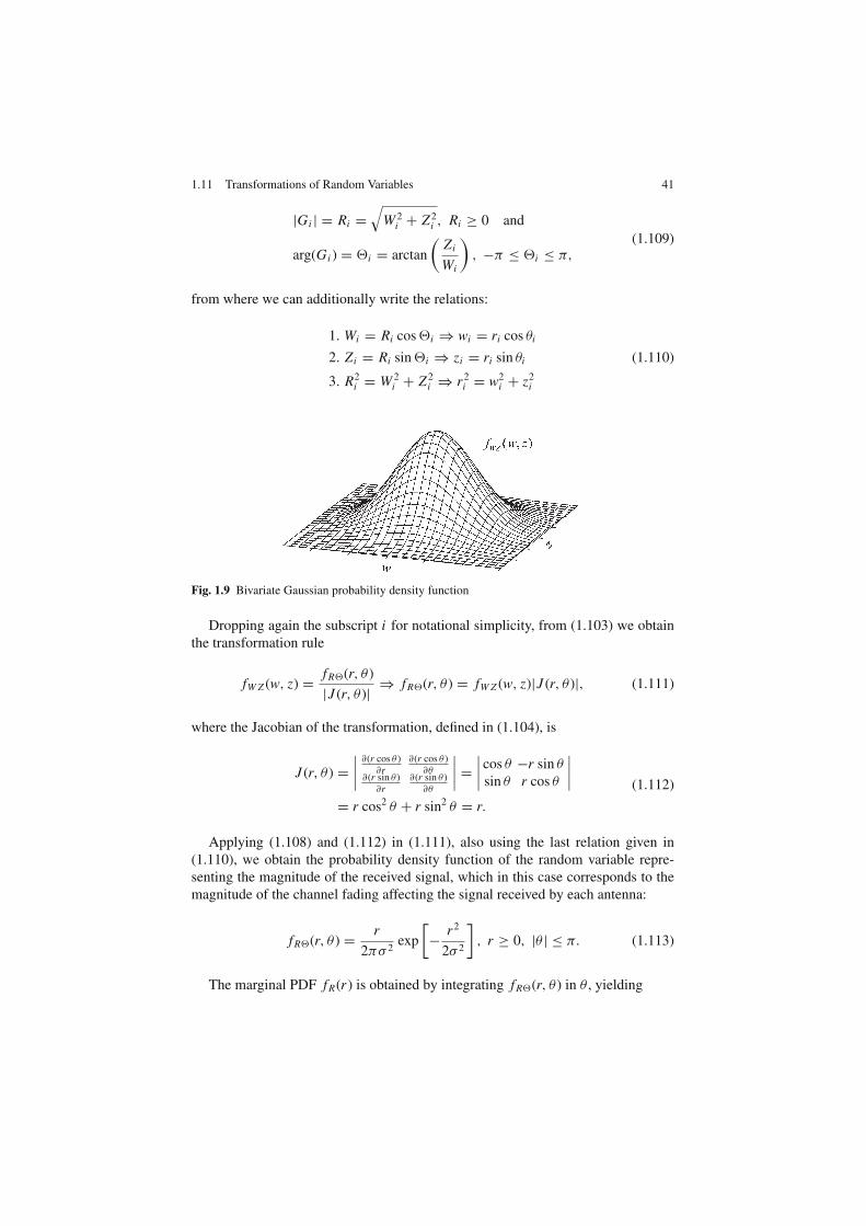
1.11 Transformations of Random Variables 41
|G i | = Ri =√
W 2i + Z2
i , Ri ≥ 0 and
arg(G i ) = Θi = arctan
(
Z i
Wi
)
, −π ≤ Θi ≤ π,
(1.109)
from where we can additionally write the relations:
1. Wi = Ri cos Θi ⇒ wi = ri cos θi
2. Z i = Ri sin Θi ⇒ zi = ri sin θi (1.110)
3. R2i = W 2
i + Z2i ⇒ r2
i = w2i + z2
i
Fig. 1.9 Bivariate Gaussian probability density function
Dropping again the subscript i for notational simplicity, from (1.103) we obtain
the transformation rule
fW Z (w, z) =fRΘ(r, θ )
|J (r, θ )|⇒ fRΘ(r, θ ) = fW Z (w, z)|J (r, θ )|, (1.111)
where the Jacobian of the transformation, defined in (1.104), is
J (r, θ ) =∣
∣
∣
∣
∂(r cos θ)∂r
∂(r cos θ)∂θ
∂(r sin θ)∂r
∂(r sin θ)∂θ
∣
∣
∣
∣
=∣
∣
∣
∣
cos θ −r sin θ
sin θ r cos θ
∣
∣
∣
∣
= r cos2 θ + r sin2 θ = r.
(1.112)
Applying (1.108) and (1.112) in (1.111), also using the last relation given in
(1.110), we obtain the probability density function of the random variable repre-
senting the magnitude of the received signal, which in this case corresponds to the
magnitude of the channel fading affecting the signal received by each antenna:
fRΘ(r, θ ) =r
2πσ 2exp
[
−r2
2σ 2
]
, r ≥ 0, |θ | ≤ π. (1.113)
The marginal PDF fR(r ) is obtained by integrating fRΘ(r, θ ) in θ , yielding
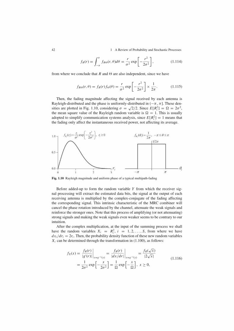
42 1 A Review of Probability and Stochastic Processes
fR(r ) =∫ π
−π
fRΘ(r, θ )dθ =r
σ 2exp
[
−r2
2σ 2
]
, (1.114)
from where we conclude that R and Θ are also independent, since we have
fRΘ(r, θ ) = fR(r ) fΘ(θ ) =r
σ 2exp
[
−r2
2σ 2
]
×1
2π. (1.115)
Then, the fading magnitude affecting the signal received by each antenna is
Rayleigh-distributed and the phase is uniformly-distributed in (−π , π ]. These den-
sities are plotted in Fig. 1.10, considering σ =√
2/2. Since E[R2i ] = Ω = 2σ 2,
the mean square value of the Rayleigh random variable is Ω = 1. This is usually
adopted to simplify communication systems analysis, since E[R2i ] = 1 means that
the fading only affect the instantaneous received power, not affecting its average.
Fig. 1.10 Rayleigh magnitude and uniform phase of a typical multipath-fading
Before added-up to form the random variable Y from which the receiver sig-
nal processing will extract the estimated data bits, the signal at the output of each
receiving antenna is multiplied by the complex-conjugate of the fading affecting
the corresponding signal. This intrinsic characteristic of the MRC combiner will
cancel the phase rotation introduced by the channel, attenuate the weak signals and
reinforce the stronger ones. Note that this process of amplifying (or not attenuating)
strong signals and making the weak signals even weaker seems to be contrary to our
intuition.
After the complex multiplication, at the input of the summing process we shall
have the random variables X i = R2i , i = 1, 2, . . . , S, from where we have
dxi/dri = 2ri . Then, the probability density function of these new random variables
X i can be determined through the transformation in (1.100), as follows:
fX (x) =fR(r )
|g′(r )|
∣
∣
∣
∣
x=g−1(y)
=fR(r )
|dx/dr |
∣
∣
∣
∣
x=g−1(y)
=fR(
√x)
|2√
x |
=1
2σ 2exp
[
−x
2σ 2
]
=1
Ωexp
[
−x
Ω
]
, x ≥ 0,
(1.116)
1.11 Transformations of Random Variables 43
where, again, we have dropped the subscripts for simplicity. The PDF in (1.116) is
a Chi-square (χ2) PDF with two degrees of freedom [13, p. 41], which corresponds
to an exponential PDF with rate parameter 1/Ω.
The mean square value of the random variable X can be obtained from the second
derivative of its moment-generating function φX (s), according to (1.61). Applying
this operation to the φX (s) given in (1.72) we obtain
E[X2] =d2φX (s)
ds2
∣
∣
∣
∣
s=0
=d2
ds2
(
1/Ω
1/Ω − s
)∣
∣
∣
∣
s=0
= 2Ω2. (1.117)
The random variable at the output of the MRC combiner will be
Y =S
∑
i=1
X i . (1.118)
At the beginning of this example we have assumed that the receiving antennas
are sufficiently apart from each other to guarantee that the signals at their outputs
are independent and, as a consequence, uncorrelated. Then, the PDF of Y can be
determined by the convolution among the PDFs of X i . Since this represents a hard
mathematical problem, we resort to the property given in (1.92), which states that
the characteristic function of a sum of independent random variables is the product
of the corresponding characteristic functions. Moreover, if the random variables are
also identically-distributed, according to (1.93) the characteristic function of the
sum of S random variables is the S-th power of the characteristic function of one of
the random variables considered in the sum:
ψY ( jω) = [ψX ( jω)]S. (1.119)
According to (1.58), the probability density function of the random variable at
the output of the MRC combiner can be determined through the inverse transform
fY (y) =1
2π
∫ ∞
−∞e− jωy[ψX ( jω)]Sdω, (1.120)
where
ψX ( jω) =∫ ∞
−∞e jωx fX (x)dx =
∫ ∞
0
1
Ωexp
(
−x
Ω
)
e jωx dx . (1.121)
From Chap. 2, Table 2.4, we have the Fourier transform pair
exp(−αt)u(t), α > 0 1
α + j2π f. (1.122)
44 1 A Review of Probability and Stochastic Processes
By analogy to (1.122) and recalling the fact that (1.121) has the opposite signal
of the true Fourier transform, we obtain
ψX ( jω) =1
Ω
∫ ∞
−∞e−x/Ωu(x)e jωx dx =
1/Ω
1/Ω − jω=
1
1 − jωΩ. (1.123)
Then, applying (1.119),
ψY ( jω) = [ψX ( jω)]S =1
(1 − jωΩ)S. (1.124)
With this result in (1.120) we have
fY (y) =1
2π
∫ ∞
−∞e− jωy(1 − jωΩ)−Sdω. (1.125)
From [9, p. 170] and [10, p. 116], the probability density function and the char-
acteristic function of a gamma random variable are respectively given by
fY (y) =λ(λy)α−1e−λy
Γ(α), y ≥ 0, and
ψY ( jω) =λα
(λ − jω)α.
(1.126)
Comparing the characteristic function in (1.126) with (1.124) we can find that
λ = 1/Ω and α = S in the gamma distribution. Then, with these results in (1.126),
the PDF of the random variable at the output of the MRC is finally obtained:
fY (y) =yS−1e−y/Ω
ΩS(S − 1)!, y ≥ 0, (1.127)
where we have used the relation Γ(S) = (S − 1)!, valid for S > 0 and integer.
The PDF in (1.127) is a special form of the gamma PDF and is very similar to a
Chi-square (χ2) distribution with 2S degrees of freedom.
As a complementary analysis, let us determine the mean and the mean square
value of the random variable Y . They are given respectively by:
E[Y ] =∫ ∞
−∞y fY (y)dy =
1
ΩS(S − 1)!
∫ ∞
0
ySe−y/Ωdy and
E[Y 2] =∫ ∞
−∞y2 fY (y)dy =
1
ΩS(S − 1)!
∫ ∞
0
yS+1e−y/Ωdy.
(1.128)
From Appendix A.4 we have the definite integral

1.11 Transformations of Random Variables 45
∫ ∞
0
yne−aydy =n!
an+1, a > 0, n = 0, 1, 2, . . . . (1.129)
Applying this result in (1.128) we obtain, after some simplifications,
E[Y ] = SΩ and
E[Y 2] = S(S + 1)Ω2.(1.130)
As a final analysis, let us determine the ratio between the average signal power
and the average noise power at the MRC combiner output. We start this analysis by
defining the magnitude of a new random variable at each combiner input as a Ri ,
where a is the random variable corresponding to the magnitude of the transmitted
signal. We also denote the normalized (over a 1 ohm load) instantaneous signal
power at the combiner’s output as P and the normalized average noise power in
each combiner input as η. Then, the instantaneous power is
P =
[
S∑
i=1
(a Ri )Ri
]2
= a2
(
S∑
i=1
R2i
)2
. (1.131)
The normalized instantaneous noise power at the combiner’s output will be
N =S
∑
i=1
ηR2i = η
S∑
i=1
R2i . (1.132)
The average signal-to-noise ratio (SNR) is then
〈SNR〉 = E
[
P
N
]
= E
a2
(
S∑
i=1
R2i
)2 /
η
S∑
i=1
R2i
= E
[
a2
S∑
i=1
R2i
/
η
]
=S
∑
i=1
E[(a Ri )2/η] =
S∑
i=1
〈SNRi 〉,
(1.133)
where E[(a Ri )2/η] is the average signal-to-noise ratio in each of the combiner’s
input. Then, with the result given in (1.133) we conclude that the average SNR
at the MRC combiner’s output is the sum of the signal-to-noise ratios in the
combiner’s inputs. We now are able to understand why the use of a combiner
can bring lower probabilities of decision errors by the receiver’s signal processing
block. We accomplish this with the help of the next computer simulation.
46 1 A Review of Probability and Stochastic Processes
Simulation 1.4 – A Communication System Analysis
File – CD drive:\Simulations\Probability\MRC.vsm
Default simulation settings: Frequency = 100 Hz; End = 1,000
seconds. Second moment of the Rayleigh random variables
E[R2] = 1.5.
This experiment aims at simulating the scenario described in Example 1.5. The
system shown in Fig. 1.8 is partially implemented using VisSim/Comm. The trans-
mitted signals were simulated by constants ai = a = 1, permitting that the varia-
tions observed in the received signal are attributed to the channel fading Ri . Three
received signals are being generated to simulate the use of S = 3 receiving antennas.
Each of these signals is affected by a multiplicative Rayleigh fading with config-
urable mean square value E[R2] = Ω = 2σ 2. The phase rotation component of the
fading did not need to be considered, since we are assuming that the MRC combiner
would cancel it off anyway. The received signals enter the MRC combiner to form
the random variable Y at the combiner’s output.
Histograms and moments estimates are generated for one of the Rayleigh fading
random variables (Ri ), for one of the summing inputs inside the MRC combiner
(X i ) and for the MRC output random variable (Y ).
Average signal-to-noise ratio (SNR) estimates are also computed and that is the
reason for the repeated implementation of the combiner in the lower part of the sim-
ulation worksheet, where we have only Gaussian noise sources as the MRC input.
In other words, we need two systems to analyze signal and noise separately.
The upper SNR measurement corresponds to the output of the combiner and the
average SNR is estimated according to
〈SNR〉 = E
a2
(
S∑
i=1
R2i
)2 /
η
S∑
i=1
R2i
, (1.134)
where η = 1 is the average noise power in each of the MRC inputs. Observe the
simulation diagram and note that the MRC output corresponds exactly to the square-
root of the numerator in (1.134). Note also that, since a = 1, the value at the MRC
output times the average noise power in one of its inputs gives the instantaneous
noise power at the combiner’s output. Have a look inside the corresponding SNR
estimation block and try to associate the operations with (1.134).
The expected value estimation blocks in this simulation are applying two con-
cepts not yet discussed in this chapter. For now it suffices to know that in some
cases statistical averages can be realized through time averages. We shall present
this concept in more detail in the study of ergodic random processes. Moreover,
these time averages are being estimated here through sample averages, a concept
also treated in more detail later on in this chapter.
Continuing the analysis of the simulation diagram, the intermediate SNR mea-
surement is estimating the average signal-to-noise ratio at one of the combiners’
inputs. It is performing the operation

1.12 Parameter Estimation via Sample Mean 47
〈SNRi 〉 = E[
(a Ri )2/η
]
. (1.135)
Analyze the operations inside this block and confirm the realization of (1.135).
The SNR estimation at the bottom of the worksheet is a wrong SNR measure-
ment. It is dividing the average signal power by the average noise power. Although
this measurement seems to be intuitively satisfying, we must not forget that a given
instantaneous fading magnitude affects simultaneously the signal and the noise com-
ponents. Separate averages do not take this fact into account and, as a consequence,
produce incorrect SNR estimates.
Run the simulation using the default settings. After it is finished, observe the
estimated SNR at one of the combiner’s inputs and compare the result with the SNR
at the combiner’s output. Note that the output SNR is approximately three times the
input SNR, since S = 3. Compare this result with the theoretical expected value
given in (1.133). Observe also that the wrong SNR estimation has indeed produced
an incorrect result.
Still using the default settings open the “histogram and moments” block. Run the
simulation and observe the shapes of the histograms: the upper one resembles the
Rayleigh PDF of Ri given in (1.114). The intermediate one resembles the exponen-
tial PDF of X given in (1.116), and the histogram at the bottom shows the shape of
the PDF given in (1.127), which corresponds to the gamma random variable Y at
the output of the combiner. The mean and second moment for each of these random
variables are expected to be:
1. E[Ri ] = σ√
π/2 =√
Ωπ/4 =√
1.5π/4 ∼= 1.085
2. E[R2i ] = 2σ 2 = Ω = 1.5
3. E[X i ] = 1/λ = Ω = 1.5
4. E[X2i ] = 2Ω
2 = 2 × 1.52 = 4.5
5. E[Yi ] = SΩ = 3 × 1.5 = 4.5
6. E[Y 2i ] = S(S + 1)Ω2 = 3(3 + 1)1.52 = 27.
(1.136)
Compare the above theoretical results with those estimated in the simulation.
Explore inside the individual blocks. Try to understand how they were implemented.
Create and investigate for yourself new situations and configurations of the simula-
tion parameters and try to reach your own conclusions.
1.12 Parameter Estimation via Sample Mean
When dealing with random data, it is common to have no a priori information about
the statistical properties of the samples we have. The analysis of such data would

48 1 A Review of Probability and Stochastic Processes
be impossible if the samples did not show some average behavior when more and
more data are analyzed.
In this section we present the concept of sample mean. It is a tool that permits the
average behavior of the data to be unveiled, allowing for the estimation of some sta-
tistical properties about the samples. Additionally, this estimation is always attached
to some degree of uncertainty that can be controlled through the analysis of confi-
dence intervals, a topic also covered in this section.
1.12.1 The Sample Mean
Let the random variable Y correspond to the sum of n independent and identically
distributed random variables X1, X2, . . ., X i , . . ., Xn . The sample mean is another
random variable defined according to
Mn(X ) =1
n
n∑
i=1
X i . (1.137)
The mean and the variance of the sample mean are given respectively by
E[Mn(X )] = E[X ] and
var[Mn(X )] =var[X ]
n.
(1.138)
From the mean in (1.138) we conclude that the sample mean is an unbiased4
estimator for E[X ]. From the variance in (1.138) we conclude that the value of the
sample mean converges to E[X ] as n goes to infinity.
Note that there is a connection between the sample mean and the central limit
theorem: as n increases, Mn(X ) approaches a Gaussian random variable with mean
E[X ] and variance going towards zero.
The sample mean is useful not only for estimating the first moment of a random
variable. For this reason it is sometimes called sample average. For example, if we
compute the sample average Mn(X2) = (X21 + X2
2 + . . . + X2i + . . . + Xn)/n we are
estimating the second moment of the random variable X . This gives to the sample
mean a broader use in practical applications, as we shall see below with the help of
an example.
Example 1.6 – By observing the quotation of the coffee bag from the stock
exchange in different periods of 100 days we shall obtain values that can be associ-
ated to the random variables X1, X2, . . ., X i , . . ., X100. Similarly, by observing the
4 An estimate R of the parameter r is said to be unbiased if E[R] = r . If E[R] 6= r the estimatoris said to be biased [18, p. 280].
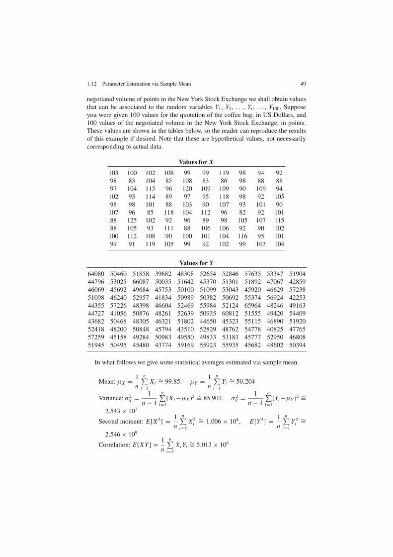
1.12 Parameter Estimation via Sample Mean 49
negotiated volume of points in the New York Stock Exchange we shall obtain values
that can be associated to the random variables Y1, Y2, . . ., Yi , . . ., Y100. Suppose
you were given 100 values for the quotation of the coffee bag, in US Dollars, and
100 values of the negotiated volume in the New York Stock Exchange, in points.
These values are shown in the tables below, so the reader can reproduce the results
of this example if desired. Note that these are hypothetical values, not necessarily
corresponding to actual data.
Values for X
103 100 102 108 99 99 119 98 94 92
98 85 104 85 108 83 86 98 88 88
97 104 115 96 120 109 109 90 109 94
102 95 114 89 97 95 118 98 92 105
98 98 101 88 103 90 107 93 101 90
107 96 85 118 104 112 96 82 92 101
88 125 102 92 96 89 98 105 107 115
88 105 93 111 88 106 106 92 90 102
100 112 108 90 100 101 104 116 95 101
99 91 119 105 99 92 102 99 103 104
Values for Y
64080 50460 51858 39682 48308 52654 52846 57635 53347 51904
44796 53025 66087 50035 51642 45370 51301 51892 47067 42859
46069 45692 49684 45753 50100 51099 53043 45920 46629 57238
51098 46240 52957 41834 50989 50382 50692 55374 56924 42253
44355 57226 48398 46604 52469 55984 52124 65964 48246 49163
44727 41056 50876 48261 52639 50935 60812 51555 49420 54409
43682 50468 48305 46321 51802 44650 45323 55115 46890 51920
52418 48200 50848 45794 43510 52829 48762 54778 40825 47765
57259 45158 49284 50983 49550 49833 53183 45777 52950 46808
51945 50495 45480 43774 59169 55923 55935 45682 48602 50394
In what follows we give some statistical averages estimated via sample mean.
Mean: µX =1
n
n∑
i=1
X i∼= 99.85, µY =
1
n
n∑
i=1
Yi∼= 50,204
Variance: σ 2X =
1
n − 1
n∑
i=1
(X i −µX )2 ∼= 85.907, σ 2Y =
1
n − 1
n∑
i=1
(Yi −µY )2 ∼=
2.543 × 10⁷
Second moment: E[X2] =1
n
n∑
i=1
X2i
∼= 1.006 × 10⁴, E[Y 2] =1
n
n∑
i=1
Y 2i
∼=
2.546 × 10⁹
Correlation: E[XY ] =1
n
n∑
i=1
X i Yi∼= 5.013 × 10⁶

50 1 A Review of Probability and Stochastic Processes
Covariance: cov[X, Y ] =1
n − 1
n∑
i=1
(X i − µX )(Yi − µY ) ∼= 44.086
Correlation coefficient: ρ =cov[X, Y ]√
σ 2X
√
σ 2Y
∼= 9.53 × 10⁻⁴
Comments on the Above Results:
• Note that we have made the division by n − 1 instead of n in the estimation of
the variance and of the covariance, since the division by n would produce biased
estimators [18, p. 284]. However, for large n the difference between the biased
and the unbiased estimators is small and the use of n − 1 or n is indifferent.
Moreover, if we know the true values of mean inside the variance and covariance
computations, the division by n produces unbiased estimators.
• We are not able to precisely estimate the shapes of the probability density func-
tions of the random variables X and Y through histograms, since the sample size
is small (see Example 1.4 for more details on this subject).
• Suppose that we want to use the New York Stock Exchange data as a reference for
predicting the variations in the price of a coffee bag. From the averages obtained
we notice that, despite of the high correlation and apparently high covariance, the
correlation coefficient is approximately zero, indicating that X and Y are uncor-
related. We would have inferred erroneously if we have said that an increase in
the New York Stock Exchange quotation would probably have been accompanied
by an increase in the prince of the coffee bag.
1.12.2 The Confidence Interval on the Sample Mean
In this subsection we shall quantify the precision of the parameter estimation made
via sample mean. This quantification will be made through the confidence interval
and the confidence coefficient.
The analysis of confidence interval is not restricted to those cases mentioned in
this section. The reader is encouraged to consult the book edited by H. Pham [12]
for a broader treatment on this and many other related subjects.
The Chebyshev inequality [9, p. 181] states that, given a random variable X with
expected value E[X ] and variance var[X ], for any positive number c,
P[|X − E[X ]| ≥ c] ≤var[X ]
c2. (1.139)
Applying this inequality to the definition of the sample mean we obtain
P[|Mn(X ) − E[X ]| ≥ c] ≤var[Mn(X )]
c2=
var[X ]
nc2= α. (1.140)
1.12 Parameter Estimation via Sample Mean 51
This inequality states that the probability that the sample mean is distant from
the true mean more than a value c is less then or equal to α. In other words, at least
100 × (1 − α)% of the values of the sample mean will be in the range (E[X ] − c,
E[X ] + c). Yet another interpretation, the value of the sample mean will be in the
range (E[X ] − c, E[X ] + c) with probability (1 − α).
The length 2c is called confidence interval and the value (1 − α) is called con-
fidence coefficient. Then, the size of the confidence interval gives the precision we
want on the sample mean and the confidence coefficient gives us an idea about how
many values of the sample mean will be in the confidence interval. The sample size,
n, governs the overall desired precision.
The confidence interval obtained via the Chebyshev inequality is somewhat loose
or pessimistic in many cases. This means that, for most of the applications, more
than 100 × (1 −α)% of the values of the sample mean will be within the confidence
interval 2c. However, the Chebyshev inequality approach is useful when we do not
know a priori the distribution of the data.
Fortunately, most of the cases related to communication systems can resort to
the central limit theorem and consider that the sample mean is Gaussian-distributed.
This is often the case in Monte Carlo simulations, where a large number or random
values are computer-generated according to the random phenomena of interest and
the desired parameter is estimated via sample mean. The following example aims at
clarifying these statements.
Example 1.7 – In this example we shall analyze the confidence interval on the
estimate of the bit error probability Pb in a digital communication system. We start
by recalling that Pb can be computed through the relative frequency interpretation
of probability, that is,
Pb = limn→∞
nE
n, (1.141)
where nE is the number of bits in error and n is the total number of transmitted bits.
The estimate of Pb is made in practice through a finite sample size and, in this case,
Pb is usually referred to as the bit error rate (BER), which is given by
BER =nE
n. (1.142)
A well-known rule-of-thumb states that we shall have a “good” estimate of the
BER if we wait for the occurrence of 100 bit errors. The aim of this example is
to obtain a better judgment on how good is the BER estimation, in the light of the
confidence interval analysis.
A usual measurement of the precision of an estimate made via sample mean is
known as the normalized standard error standard error, which can be defined by

52 1 A Review of Probability and Stochastic Processes
Sµ =√
σ 2e
µ, (1.143)
where the numerator corresponds to the square root of the estimator error variance,
and is called the standard error of this estimator. For the present context, the nor-
malized standard error can be written as
SµX=
√var[Mn(X )]
µX
=σX√nµX
. (1.144)
We know that the number of errors in a block of n bits has a binomial distribution
with parameters n and p = Pb. Then, the sample mean Mn(X ) corresponds to the
desired BER estimate. In this case we can rewrite the normalized standard error,
yielding
Sp =√
p(1 − p)/n
p=
√
1 − p
np. (1.145)
Since the probability of error is a small quantity (compared to 1) in real commu-
nication systems, we can approximate (1.145) according to
Sp∼=
1√
np. (1.146)
If we expect 100 errors in a block of n bits and the probability of error is p, then
the mean of the corresponding binomial random variable is np = 100. With this
value in (1.146) we have Sp = 0.1. In light of (1.144), Sp = 0.1 means that the
standard deviation of the sample mean is 0.1p.
Considering a confidence coefficient of 0.9, in what follows we determine the
confidence interval, assuming that, if np = 100 and p is small, n will be sufficiently
large, allowing us to approximate the binomial sample mean to a Gaussian random
variable. First we recall the calculation of the area under a Gaussian tail given in
(1.79), repeated here for convenience:
P[X ≥ γ ] =1
2erfc
(
γ − µ
σ√
2
)
. (1.147)
Additionally we observe that
P[|Mn(X ) − E[X ]| ≥ c] = α = 2P[Mn(X ) ≥ (E[X ] + c)]. (1.148)
Applying this relation in (1.147) we obtain
α = erfc
(
c√
var[Mn(X )]√
2
)
. (1.149)

1.12 Parameter Estimation via Sample Mean 53
Using the confidence coefficient (1 − α) = 0.9 and the standard deviation of the
sample mean of 0.1p we have
0.1 = erfc
(
c
0.141p
)
. (1.150)
From the computation of the complementary error function we obtain
c
0.141p∼= 1.16309 ⇒ c = 0.164p. (1.151)
From the above result we conclude that, since the confidence coefficient is
0.9, around 90% of the values of the estimated BER will be in the range (Pb −0.164Pb, Pb + 0.164Pb). Since normally we do not know the value of Pb, by
waiting for 100 bit errors we expect that around 90% of the estimated BER val-
ues will be distant from the true value of Pb in a maximum of ±16.4%. This
is indeed a quite good estimate, as subjectively stated at the beginning of this
example.
Simulation 1.5 – Confidence Interval on BER Estimations
File – CD drive:\Simulations\Probability\Confidence BER.vsm
Default simulation settings: Frequency = 1 Hz; End = 500,000
seconds. Number of bit errors: 100. Theoretical probability of error:
0.02. Confidence coefficient: 0.9.
In this experiment we consider the bit error rate (BER) estimation problem given in
Example 1.7, and investigate the convergence of the estimation using a confidence
interval analysis. Open the simulation file indicated in the header and follow the
description given below.
Data bits are randomly generated at 1 bit per second. These bits are transmit-
ted through a binary symmetric channel whose behavior was already described in
Example 1.2. The crossover probability of the BSC channel can be configured to
simulate different values for the bit error probability Pb. At the output of the BSC,
the received bits are compared with the transmitted ones and an estimate of the BER
is made according to (1.142), where the number of expected bits in error per blocks,
nE , can be configured and n is the number of transmitted bits, calculated according
to n = nE/Pb.
A histogram of the estimated BER is computed and a time plot registers the
confidence interval limits and the estimated BER values. These limits are computed
according to (1.149), given the configurable confidence coefficient (1 − α).
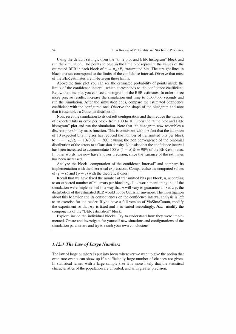
54 1 A Review of Probability and Stochastic Processes
Using the default settings, open the “time plot and BER histogram” block and
run the simulation. The points in blue in the time plot represent the values of the
estimated BER in each block of n = nE/Pb transmitted bits. The straight lines in
black crosses correspond to the limits of the confidence interval. Observe that most
of the BER estimates are in-between these limits.
Above the time plot you can see the estimated probability of points inside the
limits of the confidence interval, which corresponds to the confidence coefficient.
Below the time plot you can see a histogram of the BER estimates. In order to see
more precise results, increase the simulation end time to 5,000,000 seconds and
run the simulation. After the simulation ends, compare the estimated confidence
coefficient with the configured one. Observe the shape of the histogram and note
that it resembles a Gaussian distribution.
Now, reset the simulation to its default configuration and then reduce the number
of expected bits in error per block from 100 to 10. Open the “time plot and BER
histogram” plot and run the simulation. Note that the histogram now resembles a
discrete probability mass function. This is consistent with the fact that the adoption
of 10 expected bits in error has reduced the number of transmitted bits per block
to n = nE/Pb = 10/0.02 = 500, causing the non convergence of the binomial
distribution of the errors to a Gaussian density. Note also that the confidence interval
has been increased to accommodate 100 × (1 − α)% = 90% of the BER estimates.
In other words, we now have a lower precision, since the variance of the estimates
has been increased.
Analyze the block “computation of the confidence interval” and compare its
implementation with the theoretical expressions. Compare also the computed values
of (p − c) and (p + c) with the theoretical ones.
Recall that we have fixed the number of transmitted bits per block, n, according
to an expected number of bit errors per block, nE . It is worth mentioning that if the
simulation were implemented in a way that n will vary to guarantee a fixed nE , the
distribution of the estimated BER would not be Gaussian anymore. The investigation
about this behavior and its consequences on the confidence interval analysis is left
to an exercise for the reader. If you have a full version of VisSim/Comm, modify
the experiment so that nE is fixed and n is varied accordingly. Hint: modify the
components of the “BER estimation” block.
Explore inside the individual blocks. Try to understand how they were imple-
mented. Create and investigate for yourself new situations and configurations of the
simulation parameters and try to reach your own conclusions.
1.12.3 The Law of Large Numbers
The law of large numbers is put into focus whenever we want to give the notion that
even rare events can show up if a sufficiently large number of chances are given.
In statistical terms, with a large sample size it is more likely that the statistical
characteristics of the population are unveiled, and with greater precision.
1.13 Generation of Random Numbers 55
The weak law of large numbers is mathematically stated as:
1. limn→∞
P[|Mn(X ) − µX | ≥ c] = 0
2. limn→∞
P[|Mn(X ) − µX | < c] = 1.(1.152)
The first expression in (1.152) states that Mn(X ) − µX tend to be small with
high probability as n is increased. It does no state that Mn(X ) = µX with high
probability. It also does not state that P[|Mn(X ) − µX | ≥ c] = 0. Both a non-zero
value for c and for the probability are necessary here, despite of the fact that by
increasing n it is possible to make both as small as we want. The second expression
in (1.152) states that Mn(X ) converges to µX when n is increased. This is know as
probabilistic or stochastic convergence.
The strong law of large numbers can be written as
P[
limn→∞
Mn(X ) = µX
]
= 1. (1.153)
It means that Mn(X ) converges to µX with probability 1. It also means that the
sample mean does not converge to any another value different from µX .
1.13 Generation of Random Numbers
Currently, research and development activities in engineering, especially in commu-
nication systems engineering, make extensive use of computer simulations. More-
over, since most of the systems created or analyzed through engineering tools are
affected by some random phenomena, it is of major importance that the computer
simulation of such systems is able to reproduce these random phenomena with accu-
racy and, preferably, in a short time frame.
Usually, simulations are based on Monte Carlo methods in which random (actu-
ally pseudo-random) numbers generation is the most crucial part [2]. In essence, in
Monte Carlo methods a large amount of these numbers is generated to simulate the
random variables within the system and to permit the estimation of system parame-
ters through sample averages.
In this section we present some algorithms for generating random numbers.
These algorithms will be studied without a detailed analysis about the goodness-
of-fit of the results. For a deeper treatment on the subject, the interested reader is
referred to the book by J. E. Gentle [3], where special attention is given to the
assessment of the quality of random numbers generators. This assessment can be
made necessary since, for example, if the shape of a histogram resembles the proba-
bility distribution of a desired random variable, it is not guaranteed that all statistical
properties of the random variable are being reproduced by the generated random
numbers.

56 1 A Review of Probability and Stochastic Processes
1.13.1 Congruential Methods
In a congruential method, each generated number is determined by its predecessor
by means of a function (not necessarily linear) followed by a modular operation.
For example, in the multiplicative congruential method we have
Zk = αZk−1 mod M, Zk = 1, 2, . . . , M − 1, (1.154)
where α is called the multiplier, M is the modulus and Z0 6= 0 is the seed of the
generator. The congruence function (x mod y) returns the remainder on dividing x
by y.
The congruential method is able to generate a uniformly-distributed sequence of
pseudo-random numbers between 1 and M − 1. We say that the sequence will be
pseudo-random since it will repeat itself after its period. This period depends on the
choice of α and M and its maximum value is M − 1.
If M is very large and we divide the resultant numbers by M − 1, we will have
the generation of a uniform random variable in the interval (0, 1]. The greater the
value of M , the closer to zero the smallest number will be.
A commonly used modulus is the Mersenne prime 231 −1, and a commonly used
multiplier is 75 [3, p. 13]. The resultant sequence will have a period of 2,147,483,646
numbers, a value that is sufficiently large for most applications. In other words, the
sequence will not repeat itself during most of the simulations of practical interest.
With such a large value of M , if we divide the generated numbers by M − 1, the
smallest resultant number will be indeed very close to 0.
The importance of generating random numbers with uniform distribution is that
random numbers having other distributions are usually generated from uniformly-
distributed numbers, as we shall see in the sequel.
1.13.2 Inverse CDF Method
The inverse cumulative distribution function (CDF) method is one of the sim-
plest manners for generating continuous or discrete random variables. It is better
explained through an illustration, as shown in Fig. 1.11. Uniformly-distributed ran-
dom numbers U in the range (0, 1] are generated and the random numbers X with
the desired distribution are obtained from the inverse of its cumulative distribution
function for a given value of U .
For discrete random variables, the method is even more straightforward. The
probabilities of the values of X determine comparison thresholds and a given
value of X is generated if U is within a specific range of values. For example,
the value 3 for the random variable X in Fig. 1.11(b) is generated whenever a
value of U is generated in the range [0.4, 0.7). Note that a value of U in this
range will happen with probability 0.3, which will correspond to the probability
P[X = 3].
Other continuous distributions with CDF FY (y) can be used instead of the uni-
form, though uniform random numbers are used in the majority of cases.

1.13 Generation of Random Numbers 57
Fig. 1.11 The inverse CDF method for continuous (a), and discrete (b) random variables
We can generalize the inverse CDF method and write that
X = F−1X [FY (Y )]. (1.155)
The inverse CDF method is simple in all cases where it is simple to find the
inverse CDF of the desired random variable. The method is summarized below:
1. Generate a random variable U having a uniform distribution in (0, 1).
2. Make X = F−1X (U ), where F−1
X (U ) is the value of x when FX (x) = U .
1.13.3 Acceptance/Rejection Methods
An acceptance/rejection method generates a random variable X with probability
density fX (x) based on the realizations of another random variable Y with PDF
fY (y), preferably similar to fX (x).
The following algorithm corresponds to one of the acceptance/rejection methods,
which is used to operate from uniformly-distributed random numbers (Fig. 1.12
illustrates examples of the PDFs involved):
1. Choose a scaled PDF c fY (y) in a way that the total area of the desired PDF fX (x)
lies inside the area of c fY (y).
2. Generate a random number Y with density fY (y).
3. Generate a uniformly-distributed random number U in the interval (0, c fY (Y )].
4. If U ≤ fX (Y ), accept Y as a valid realization of X , that is X ← Y .
5. If U > fX (Y ), reject Y and go to step 2.
The idea behind an acceptance/rejection method is that sub-samples properly
selected from samples having a given distribution are stochastically equivalent to
samples from a different distribution.
To reduce the number of computations in the acceptance/rejection method, one
must ensure that the proportion of acceptances is high, which means that the area
in-between the desired and the scaled PDFs must be minimized.

58 1 A Review of Probability and Stochastic Processes
Fig. 1.12 Illustration of the acceptance/rejection method to convert a uniform random number
The acceptance/rejection method is very versatile and, unlike the inverse CDF
method, it also applies to multivariate random variables.
1.13.4 Box-Muller Method
The Box-Muller method is used to generate Gaussian random variables X and
Y from two independent and uniformly-distributed random numbers U1 and U2,
through the following relations:
1. X = cos(2πU1)
√
−2σ 2X ln(U2) + µX
2. Y = sin(2πU1)
√
−2σ 2Y ln(U2) + µY ,
(1.156)
where U1 and U2 are in the interval (0, 1], σ 2X and σ 2
Y are the variances of the desired
Gaussian random variables and µX and µY are their expected values.
Simulation 1.6 – Random Numbers Generation
File – CD drive:\Simulations\Probability\Random numbers.vsm
Default simulation settings: Frequency = 100 Hz; End = 1,000
seconds. Seed value in the uniform random variable (RV) generator:
5. Variance in the exponential RV generator: 2. Probability of success
of the Bernoulli trials in the binomial RV generator: 0.5. Variance and
mean in the Gaussian RV generator: 2 and 1, respectively.
1.13 Generation of Random Numbers 59
This experiment is intended to show examples of random numbers generation using
the methods described in this section.
A total of 100,000 numbers are generated for each random variable, using the
default simulation “end” time. The histograms and estimates of the variance and
mean are shown for each generated random variable.
In the sequel we present brief descriptions of the generators. Follow these
descriptions while analyzing inside each generator through a double click over it.
Generator A implements the multiplicative congruential method to produce
uniformly-distributed random variables in the interval (0, 1]. Specifically, it imple-
ments the expression
Zk = (231 − 2)−1(75)Zk−1mod(231 − 1), (1.157)
where the initial seed Zk−1 is configurable and k = 1, 2, . . . , 100,000.
Generator B implements the inverse CDF method to generate an exponential
random variable with configurable variance 1/λ2. For this distribution we know that
the CDF is FX (x) = 1 − e−λx . Applying the inverse CDF method we have:
u = 1 − e−λx ⇒ ln(1 − u) = −λx
⇒ X = −1
λln(1 − U ) ≡ −
1
λln(U )
(1.158)
where U is a uniformly-distributed random variable in the interval (0, 1].
Generator C also implements the inverse CDF method, but this time it produces
a binomial random variable with parameters n = 5 and configurable p. The block
diagram of this generator is shown in Fig. 1.13, where the uniform random num-
ber generation is realized by a built-in block of VisSim/Comm and the comparison
thresholds were computed according to a binomial CDF, as follows:
Tx =4
∑
k=0
(
5
x
)
px (1 − p)5−x , x = 0, 1, 2, 3, 4. (1.159)
Generator D implements the acceptance/rejection method to produce random
numbers with the “custom” desired distribution fX (x) illustrated in Fig. 1.12. This
PDF and the scaled PDF c fY (y), which is also shown in Fig. 1.12, are given by
fX (x) =
(4 − x)2/3, 2 < x < 5
0, otherwiseand
c fY (y) =
cλe−λ(y−2), y ≥ 2, c = 3, λ = 0.45
0, otherwise.
(1.160)
The algorithm for realizing the acceptance/rejection method was implemented
via Mathcad and the numbers generated were exported to VisSim/Comm via a “.dat”
file. In this algorithm, the uniform random variable U was generated by a built-in

60 1 A Review of Probability and Stochastic Processes
Fig. 1.13 Binomial random number generator: n = 5 and configurable p
function of Mathcad and the exponential random variable was generated via inverse
CDF method, by applying the mapping equation:
X = −1
λln(1 − U ) + 2. (1.161)
Finally, Generator E is implementing the Box-Muller method described by the
equations in (1.156) to generate a Gaussian random variable with configurable vari-
ance σ 2X and mean µX . The uniform random variables U1 and U2 are generated by a
built-in block of VisSim/Comm.
Now, run the simulation and compare the mean and the variance of each random
variable with the theoretical results presented in Sects. 1.8 and 1.9. It is left as
an exercise for the reader to show that the mean and the variance for the random
variable X with “custom” distribution fX (x) are 2.75 and 0.638, respectively.
Open the histogram of each random variable and run the simulation. Observe the
resultant shape of the histogram and compare it with the shape of the theoretical
probability density or mass function.
Explore inside the individual blocks. Try to understand how they were imple-
mented. Create and investigate for yourself new situations and configurations of the
simulation parameters and try to reach your own conclusions.
1.14 Random Processes
When random variables manifest in time or space we say that we have a random
process. In other words, when the realizations of the random phenomenon of interest
can be represented through waveforms with the x-axis being time or space, we say
that we have a random process.
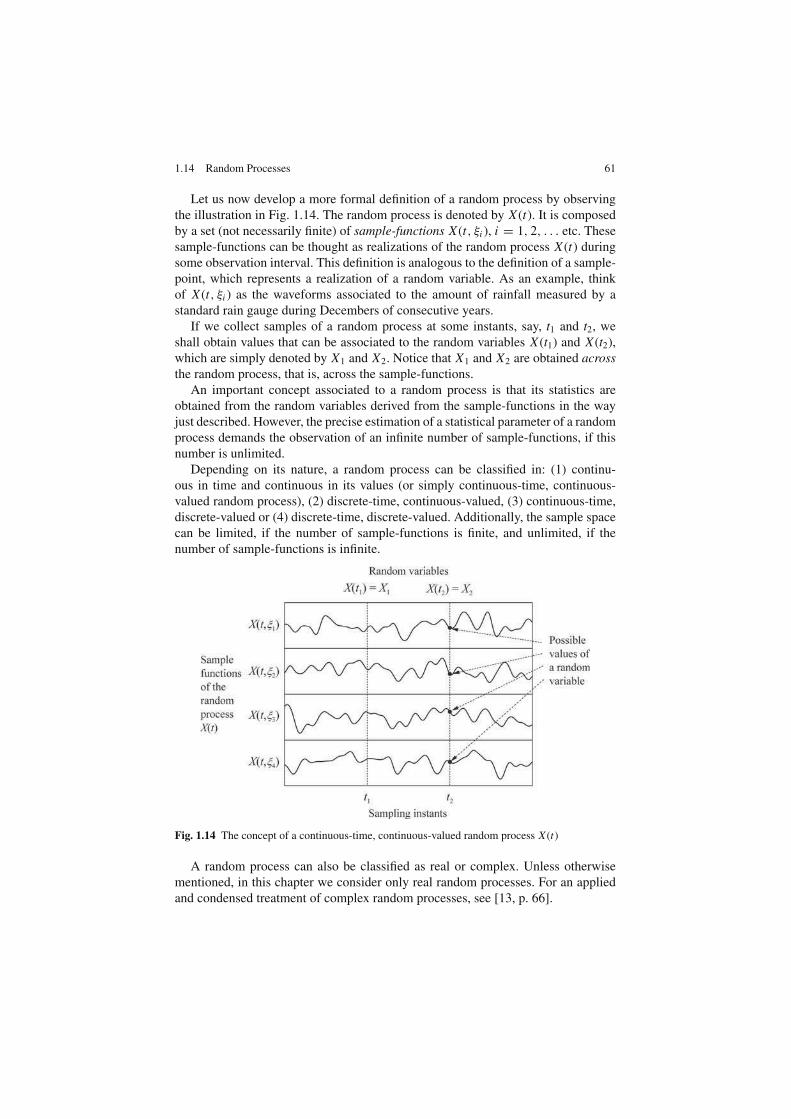
1.14 Random Processes 61
Let us now develop a more formal definition of a random process by observing
the illustration in Fig. 1.14. The random process is denoted by X (t). It is composed
by a set (not necessarily finite) of sample-functions X (t, ξi ), i = 1, 2, . . . etc. These
sample-functions can be thought as realizations of the random process X (t) during
some observation interval. This definition is analogous to the definition of a sample-
point, which represents a realization of a random variable. As an example, think
of X (t, ξi ) as the waveforms associated to the amount of rainfall measured by a
standard rain gauge during Decembers of consecutive years.
If we collect samples of a random process at some instants, say, t1 and t2, we
shall obtain values that can be associated to the random variables X (t1) and X (t2),
which are simply denoted by X1 and X2. Notice that X1 and X2 are obtained across
the random process, that is, across the sample-functions.
An important concept associated to a random process is that its statistics are
obtained from the random variables derived from the sample-functions in the way
just described. However, the precise estimation of a statistical parameter of a random
process demands the observation of an infinite number of sample-functions, if this
number is unlimited.
Depending on its nature, a random process can be classified in: (1) continu-
ous in time and continuous in its values (or simply continuous-time, continuous-
valued random process), (2) discrete-time, continuous-valued, (3) continuous-time,
discrete-valued or (4) discrete-time, discrete-valued. Additionally, the sample space
can be limited, if the number of sample-functions is finite, and unlimited, if the
number of sample-functions is infinite.
Fig. 1.14 The concept of a continuous-time, continuous-valued random process X (t)
A random process can also be classified as real or complex. Unless otherwise
mentioned, in this chapter we consider only real random processes. For an applied
and condensed treatment of complex random processes, see [13, p. 66].
62 1 A Review of Probability and Stochastic Processes
Simulation 1.7 – The Concept of Random Process
File – CD drive:\Simulations\Probability\Random process.vsm
Default simulation settings: Frequency = 100 Hz; End = 3
seconds. Auto Restart and Retain State enabled. Number of sample
functions: 10. Export to file blocks disabled. Upper (continuous-time,
continuous-valued) process selected.
This experiment aims at helping the reader to understand the concept of random pro-
cesses. It also permits that samples of the analyzed random processes are exported to
specific files. It can also be used to export data from other random processes created
by the user in substitution of the ones already provided. This feature allows the
reader to implement his own statistical data analysis from the files exported, using
the concepts presented in this chapter and well-known mathematics or spreadsheet
software tools.
Open the file indicated in the header and note that two continuous-time random
processes are being generated. The upper one is also a continuous-valued process
corresponding to a filtered noise signal. The lower process is a discrete-valued ran-
dom sequence of equally-likely rectangular pulses of amplitude ±1 and duration 1
second. The user can select the process to be analyzed by means of the “selector”
block.
Although the total number of sample-functions generated for each process can be
configured, a time plot shows the first 10 sample-functions of the selected random
process. Each sample-function lasts for 3 seconds and the complete set is generated
by an automatic restart of the simulation.
Each sample-function of the selected random process is sampled at the instants
1 and 1.4 seconds and the sample values are exported to the files “c:\X1.dat” and
“c:\X2.dat”. When the exporting option is enabled in the corresponding block, each
time you run the simulation n samples are augmented to the samples previously
stored in the file, where n is the number of sample-functions generated. If the
exporting options are not enabled, the files “c:\X1.dat” and “c:\X2.dat” are created
anyway, but no data are stored on them.
Note that the sampling process described above is being realized across the ran-
dom process, according to the theoretical concepts. These samples can be used to
estimate the statistics of a random process through ensemble averages.
A third sampling process is being realized, but along one of the sample-functions.
The resultant samples can also be used to estimate the statistics of the random
processes, but now by means of time averages. In this case, samples are taken in
0.1 second intervals during 3 seconds and the resultant values are exported to the
file “c:\X3.dat”. Whenever you run the simulation, a new set of 30n values are
augmented to the previously stored ones. By using the default settings you will have
300 samples per run.
Shortcuts are also given in the workplace to speed-up the access to the exported
files, so that you can browse, copy, delete or modify the stored data as desired.

1.14 Random Processes 63
Using the default simulation settings, open the time plot of the sample-functions
and run the simulation. Observe the similarity of the sample-functions displayed
with those shown in Fig. 1.14. Rerun the simulation and observe that you will be
presented a new set of sample-functions, as expected from the definition of a random
process. If you prefer, clear the overplot to view a new set without superimposing the
previous ones. Select the other process and repeat the instructions in this paragraph.
When finished, reset the simulation parameters to the default configuration (if you
prefer, close the file without saving and reopen it).
Now enable the file exporting process in each export block and run the simula-
tion. Through the shortcuts given, open each of the files just to get familiar with the
data displacement. Run the simulation again and notice that the number of samples
has been doubled.
This simulation will be addressed again later on in this chapter, so you can imple-
ment statistical analysis of the random processes on your own.
Explore inside the individual blocks. Try to understand how they were imple-
mented. Create and investigate for yourself new situations and configurations of the
simulation parameters and try to reach your own conclusions.
1.14.1 Stationarity Classes for Random Processes
Random processes can be classified as strict-sense stationary, wide-sense station-
ary or ergodic. A random process is said to be strict-sense stationary if the joint
distribution of any set of samples does not depend on the time origin, that is,
fX (t1),X (t2)···X (tn )(x1, x2, . . . , xn) = fX (t1+τ ),X (t2+τ )···X (tn+τ )(x1, x2, . . . , xn). (1.162)
In other words, all the statistical parameters of a strict-sense stationary random
process do not vary with any shift on the time axis.
A wide-sense random process has a constant mean and an autocovariance (or
autocorrelation) that is dependent only on the time difference t2 − t1, not on the
absolute values of t1 and t2. In mathematical terms,
µX (t) = µX , for all t , and
cov[X (t1), X (t2)] = cov[X (t2 − t1)] = K X (τ ), for all t1 and t2.(1.163)
Note that strict-sense stationarity is more restrictive than wide-sense. In what fol-
lows, unless otherwise mentioned, we shall refer to a wide-sense stationary random
process simply as a stationary process. This class of processes is of major impor-
tance for the study of communication systems theory, since most of the processes
encountered in these systems can be regarded as stationary, at least for a sufficient
long period of time. Unless otherwise mentioned, we shall consider only stationary
random processes for the rest of the presentation of this chapter.

64 1 A Review of Probability and Stochastic Processes
Another important classifications correspond to the mean-ergodic and the auto-
covariance-ergodic random processes, which correspond to sub-classes of wide-
sense random processes. For these random processes, time averages can substitute
ensemble averages, since a single realization of an ergodic process is statistically
representative of the whole process. Putting in a different way, the mean and the
correlation (or covariance) function of an ergodic random process can be obtained
from the temporal analysis of a single sample-function, instead of the analysis across
the sample-functions. Specifically,
µX =1
2T
∫ T
−T
x(t)dt and
K X (τ ) =1
2T
∫ T
−T
[x(t + τ ) − µX ][x(t) − µX ]dt
(1.164)
converge, in a mean square sense, to the mean µX and to the autocovariance K X (τ )
as T → ∞, respectively. Here x(t) is a realization or sample-function of X (t).
Many random processes encountered in communications systems analysis can be
considered ergodic, which facilitates enormously the estimation of the mean and of
the correlation or covariance functions, as we shall see in several instances through-
out the rest of this chapter.
One last classification refers to cyclostationary or periodically stationary ran-
dom processes [9, p. 525; 10, p. 373; 13, p. 75; 15, p. 458]. These are processes
in which statistical averages are periodic. These processes also arise in many situ-
ations related to communications systems analysis, for example when dealing with
linear-modulated signals.
1.14.2 Averages of Stationary Random Processes
Similar to the definition of moments of random variables, the n-th moment of a
random process X (t) is defined by
E[Xn(t)] =∫ ∞
−∞xn fX (t)(x)dx . (1.165)
In this section we study the main moments and other statistical averages of sta-
tionary random processes, with emphasis on those averages that involves one or
two processes. The analysis for multiple random processes follows by analogy to
multiple random variables and will not be presented here.
1.14.2.1 Mean and Variance
The mean and the variance of a stationary random process X (t) sampled at any
instant t are given respectively by
1.14 Random Processes 65
µX = E[X (t)] =∫ ∞
−∞x fX (t)(x)dx and
σ 2X = E
[
(X (t) − µX )2]
=∫ ∞
−∞(x − µX )2 fX (t)(x)dx .
(1.166)
From the law of large numbers, if we collect samples from a sufficiently large
number of sample-functions, the mean and the variance can be estimated through
the ensemble sample averages
µX =1
n
n∑
j=1
X (t, ξ j ) and
σ 2X =
1
n − 1
n∑
j=1
[
X (t, ξ j ) − µX
]2.
(1.167)
If the process is ergodic, the first expression in (1.164) can be applied to the
computation of the mean. Moreover, if the process is band-limited [13, p. 72] such
that it has no or almost zero frequency content for | f | > W , the following discrete-
time averages can be applied:
µX =1
n
n∑
j=1
x(t j ) and
σ 2X =
1
n − 1
n∑
j=1
[
x(t j ) − µX
]2,
(1.168)
where the values of x(t j ) are obtained by sampling a single sample-function of the
random process X (t) at a minimum rate of 2W samples per second.
1.14.2.2 Autocovariance and Autocorrelation Functions
The autocovariance and the autocorrelation functions of a random process are
defined respectively by
cov[X1, X2] = E[
(X1 − µX1)(X2 − µX2
)]
=∫ ∞
−∞
∫ ∞
−∞(x1 − µX1
)(x2 − µX2) fX1,X2
(x1, x2)dx1dx2 and
RX (t1, t2) = E[X1 X2]
=∫ ∞
−∞
∫ ∞
−∞x1x2 fX1,X2
(x1, x2)dx1dx2,
(1.169)
where we have used the shorthand notation X1 = X (t1) and X2 = X (t2).

66 1 A Review of Probability and Stochastic Processes
Now we consider only the autocorrelation function for stationary random pro-
cesses, since the autocovariance can be easily obtained by considering the adequate
subtraction of the mean of the random process, according to (1.169).
The autocorrelation of a stationary random process can be estimated through the
ensemble sample average
RX (t1, t2) = RX (t2 − t1) = RX (τ ) =1
n
n∑
j=1
X (t, ξ j )X (t + τ, ξ j ). (1.170)
If the process is ergodic, we have
RX (τ ) =1
2T
∫ T
−T
x(t + τ )x(t)dt. (1.171)
If the process is ergodic and band-limited, the following discrete-time average
can be applied:
RX (τ ) =1
n
n∑
j=1
x(t j )x(t j + τ ). (1.172)
The autocorrelation function has some important properties, as shown by:
1. RX (τ ) = RX (−τ )
2. |RX (τ )| ≤ RX (0)
3. E[X2(t)] = RX (0).
(1.173)
The autocovariance and the autocorrelation functions of a stationary random pro-
cess follow the relation
cov[X (t), X (t + τ )] = RX (τ ) − µ2X . (1.174)
If cov[X (t), X (t + τ )] = 0, the random variables obtained by sampling the ran-
dom process at instants t and t + τ are said to be uncorrelated. If RX (τ ) = 0, the
random variables obtained by sampling the random process at instants t and t + τ
are said to be orthogonal.
Example 1.8 – In Fig. 1.15 it is plotted a bipolar binary random waveform cor-
responding to a sample-function x(t) of a stationary stochastic process X (t). The
pulses of duration T are assumed to be equally-likely and the initial instant of an
entire pulse can start after td seconds, where td is a uniformly-distributed random
variable in (0, T ]. The objective of this example is to find RX (τ ), the autocorrelation
function of the random process X (t).

1.14 Random Processes 67
Fig. 1.15 Sample-function of a bipolar binary random wave
Since the pulses are equally-likely, E[X (t)] = 0. Moreover, the polarity of a
given pulse is independent of the polarity of the previous one.
In Fig. 1.15 two sampling instants are indicated, ti and tk . First let |tk − ti | ≥ T .
In this case X (tk) and X (ti ) occur in different pulses, so that
E[X (tk)X (ti )] = E[X (tk)]E[X (ti )] = 0, |tk − ti | ≥ T . (1.175)
For |tk − ti | < T , with ti < tk , X (tk) and X (ti ) will occur in the same pulse if
td < (T − |tk − ti |). In this case the correlation between X (tk) and X (ti ) will be
conditioned to the value of td . Then we have
E[X (tk)X (ti )|td ] =
A2, td < T − |tk − ti |0, otherwise.
(1.176)
To eliminate the conditioning in (1.176) we resort to the total expectance law:
E[E[X |Y ]] = E[X ]. (1.177)
Then, applying (1.177) in (1.176) we obtain
E[X (tk)X (ti )] =∫ T −|tk−ti |
0
A2 fTd(td )dtd
=∫ T −|tk−ti |
0
A2
Tdtd = A2
(
1 −|tk − ti |
T
)
.
(1.178)
Letting τ = tk − ti in (1.178), we finally obtain the autocorrelation function of
the bipolar random binary sequence:
RX (τ ) =
A2(
1 − |τ |T
)
, |τ | < T
0, otherwise.(1.179)

68 1 A Review of Probability and Stochastic Processes
This autocorrelation function is plotted in Fig. 1.16.
Fig. 1.16 Autocorrelation function of a bipolar binary random wave
1.14.2.3 Power Spectral Density (PSD)
One of the most important properties of the autocorrelation function states that
SX ( f ), the power spectral density (PSD) of the random process X (t), is determined
by the Fourier transform of the autocorrelation function RX (τ ). This transform and
the corresponding inverse are given respectively by
SX ( f ) =∫ ∞
−∞RX (τ )e− j2π f τ dτ and
RX (τ ) =∫ ∞
−∞SX ( f )e j2π f τ d f.
(1.180)
The relations in (1.180) are known as the Wiener-Khintchine relations.
From the point of view of the study of communications systems, the power spec-
tral density (PSD) is an important characteristic of a voltage or current random
process, since it reveals the frequency content of the process. In other words, it
measures the distribution of the power of a random signal in the frequency domain
and for this reason it is measured in watts/hertz.
A fast-varying random process has an autocorrelation function more concen-
trated around τ = 0, yielding a wide PSD. A slowly-varying random process has an
RX (τ ) decaying slowly with τ and, as a consequence, it has a narrowband PSD.
The PSD has some important properties:
1.
∫ ∞
−∞SX ( f )d f = RX (0) = E[X2(t)]
2. SX ( f ) = SX (− f ).
(1.181)
That is, the total average power of a voltage or current random process developed
over a 1Ω resistance, which corresponds to the second moment of the process, can
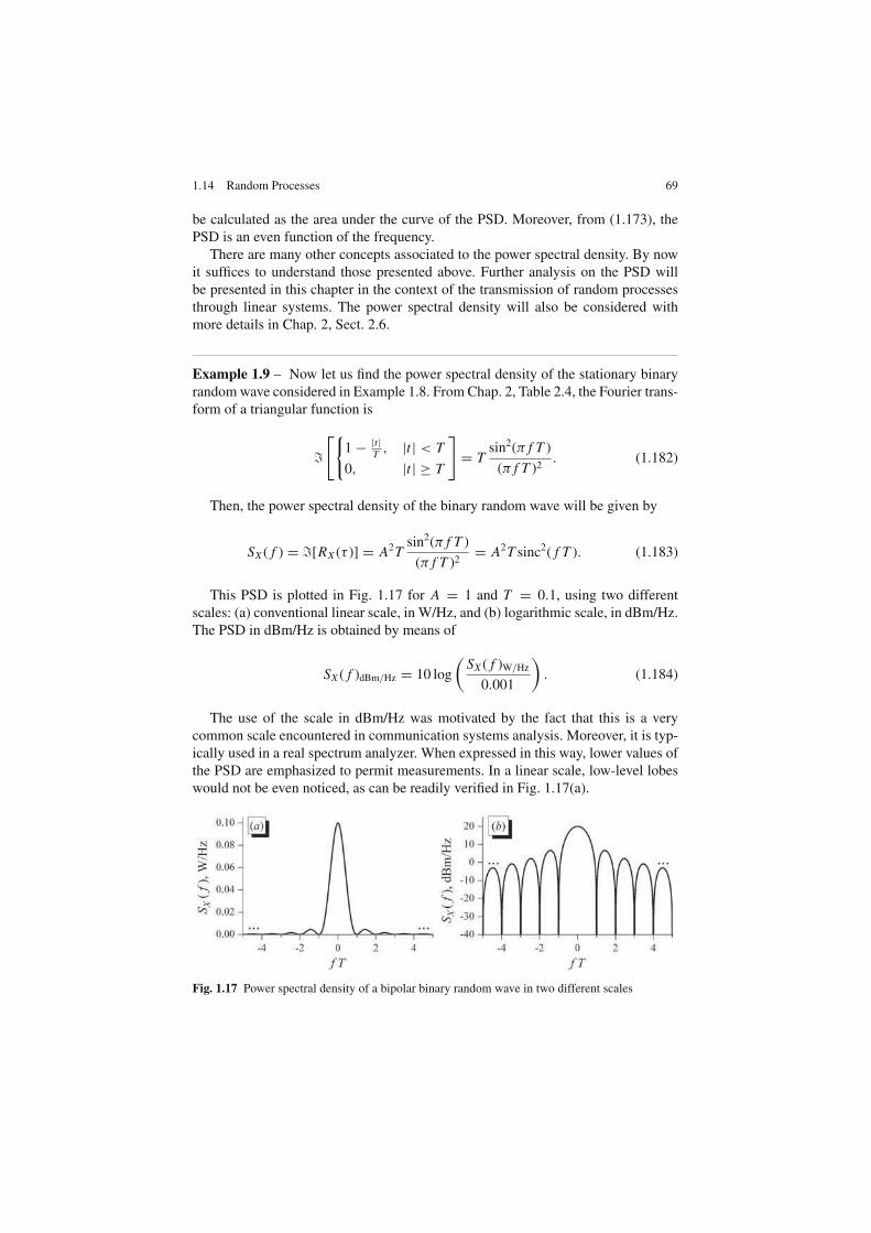
1.14 Random Processes 69
be calculated as the area under the curve of the PSD. Moreover, from (1.173), the
PSD is an even function of the frequency.
There are many other concepts associated to the power spectral density. By now
it suffices to understand those presented above. Further analysis on the PSD will
be presented in this chapter in the context of the transmission of random processes
through linear systems. The power spectral density will also be considered with
more details in Chap. 2, Sect. 2.6.
Example 1.9 – Now let us find the power spectral density of the stationary binary
random wave considered in Example 1.8. From Chap. 2, Table 2.4, the Fourier trans-
form of a triangular function is
ℑ
[
1 − |t |T
, |t | < T
0, |t | ≥ T
]
= Tsin2(π f T )
(π f T )2. (1.182)
Then, the power spectral density of the binary random wave will be given by
SX ( f ) = ℑ[RX (τ )] = A2Tsin2(π f T )
(π f T )2= A2T sinc2( f T ). (1.183)
This PSD is plotted in Fig. 1.17 for A = 1 and T = 0.1, using two different
scales: (a) conventional linear scale, in W/Hz, and (b) logarithmic scale, in dBm/Hz.
The PSD in dBm/Hz is obtained by means of
SX ( f )dBm/Hz = 10 log
(
SX ( f )W/Hz
0.001
)
. (1.184)
The use of the scale in dBm/Hz was motivated by the fact that this is a very
common scale encountered in communication systems analysis. Moreover, it is typ-
ically used in a real spectrum analyzer. When expressed in this way, lower values of
the PSD are emphasized to permit measurements. In a linear scale, low-level lobes
would not be even noticed, as can be readily verified in Fig. 1.17(a).
Fig. 1.17 Power spectral density of a bipolar binary random wave in two different scales

70 1 A Review of Probability and Stochastic Processes
From (1.173), E[X2(t)] = RX (0). Since E[X (t)] = 0, the second moment of the
process also corresponds to its average AC power. Observing Fig. 1.16 we see that
RX (0) = A2. Since A = 1 in this example, E[X2(t)] = 1 watt.
From the PSD in Fig. 1.17(a), it is apparent that most of the signal power is
concentrated in the main lobe of the frequency spectrum. Making a coarse approx-
imation of this lobe as a triangle, its area would be (2/T ) × (A2T )/2 = A2 = 1.
This result shows us that, in fact, the average power of a random process can be
determined by the area under its power spectral density.
1.14.2.4 Cross-Covariance and Cross-Correlation Functions
The cross-covariance and the cross-correlation functions follow the same reasoning
adopted for the autocovariance and the autocorrelation functions, the only difference
being the fact that, now, we are dealing with two different random processes X (t)
and Y (t), instead of one. The expressions must then reflect this.
The cross-covariance and the cross-correlation functions of two stationary ran-
dom processes follow the relation
cov[X (t), Y (t + τ )] = RXY (τ ) − µ2Xµ2
Y . (1.185)
If cov[X (t), Y (t + τ )] = 0, the random processes are said uncorrelated. If the
cross-correlation RXY (τ ) = 0, the random processes are said orthogonal. Note that
if two random processes are orthogonal, they will be uncorrelated if and only if one
of their means or both are zero.
The cross-correlation function for ergodic processes can be estimated by
RXY (τ ) =1
2T
∫ T
−T
x(t + τ )y(t)dt. (1.186)
If the processes are band-limited such that they have no or almost zero frequency
content for | f | > W , the following discrete-time average can be applied:
RXY (τ ) =1
n
n∑
i=1
x(ti )y(ti + τ ), (1.187)
where x(t j ) and y(t j + τ ) are obtained by sampling a single sample-function of the
random processes X (t) and Y (t + τ ) at a rate 2W samples per second or greater.
It is worth mentioning that if the random processes are cyclostationary, all the
statistics presented above can be computed by considering a time interval of just
one period of the processes.
1.14 Random Processes 71
Simulation 1.8 – Estimating Averages of Random Processes
File – CD drive:\Simulations\Probability\Random process.vsm
Default simulation settings: Frequency = 100 Hz; End = 3 seconds.
Auto Restart and Retain State enabled. Number of sample
functions: 10. Export to file blocks disabled. Upper (continuous-time,
continuous-valued) process selected.
In this experiment we revisit the diagram considered in Simulation 1.7, now with
the aim of obtaining some statistical averages of the simulated random processes.
Open the simulation file indicated in the header and set the number of sample-
functions to 9,000. Enable the export blocks for “X1.dat” and “X2.dat” and run
the simulation. Wait for a while until the end of the simulation. Disable the export
blocks for “X1.dat” and “X2.dat” and enable the export block for “X3.dat”. Change
the number of sample-functions to 300 and run the simulation. Now you have three
files, each having 9,000 samples: “X1.dat” has samples taken across the process
X (t) when sampled at t = 1 s, “X2.dat” has samples taken across the process X (t)
sampled at t = 1.4 s and “X3.dat” has samples taken along one sample function of
the process X (t).
As an exercise, load the above samples into a mathematical software toll, like
Mathcad, Matlab and Mathematica or into a spread-sheet like Excel. Implement the
sample averages that follow and try to obtain similar results.
(a) Ensemble mean of X (t):
µX =1
n
n∑
j=1
X (t, ξ j )
=1
n
n∑
j=1
X (1, ξ j ) =1
9000
9000∑
j=1
X1 j∼= 0.0103 (1.188)
=1
n
n∑
j=1
X (1.4, ξ j ) =1
9000
9000∑
j=1
X2 j∼= 0.01.
Note that the estimated means are essentially the same, which is a consequence
of the stationarity of the random process. Additionally, they are close to zero, the
actual mean value of the continuous-time, continuous-valued process.
(b) Time average mean of X (t):
µX =1
n
n∑
j=1
x(t j ) (1.189)

72 1 A Review of Probability and Stochastic Processes
=1
9000
9000∑
j=1
X3 j∼= −0.004.
Note that the mean obtained from the samples of a single sample-function of X (t)
is also close to the actual value, indicating that such random process is ergodic.
(c) Autocorrelation of X (t) for τ = 0.4 s:
RX (τ ) =1
n
n∑
j=1
X (t, ξ j )X (t + τ, ξ j )
=1
9000
9000∑
j=1
X (1, ξ j )X (1 + 0.4, ξ j ) (1.190)
=1
9000
9000∑
j=1
X1 j X2 j∼= −6.6 × 10⁻³.
This value indicates that the random variables X (t1) = X1 and X (t2) = X2 have
a low correlation for the value of τ = t2 − t1 = 0.4 seconds. For τ = t2 − t1 = 0
we shall find:
(d) Autocorrelation of X (t) for τ = 0:
RX (0) =1
9000
9000∑
j=1
X (1, ξ j )X (1, ξ j )
=1
9000
9000∑
j=1
X (1.4, ξ j )X (1.4, ξ j ) (1.191)
=1
9000
9000∑
j=1
X12j∼=
1
9000
9000∑
j=1
X22j∼= 1.09.
This is indeed the approximate total average power of the continuous-time,
continuous-valued random process.
(e) Time average variance of X (t):
σ 2X =
1
n − 1
n∑
j=1
[
x(t j ) − µX
]2(1.192)
=1
8999
9000∑
j=1
[
X3 j + 0.004]2 ∼= 1.04.

1.14 Random Processes 73
Note the this value makes sense, since for a zero-mean voltage random wave-
form, the DC power is zero and the total average power is equal to the AC power.
Finally, let us illustrate how a time average autocorrelation could be performed
from “X3.dat”. We need to multiply, sample-by-sample, x(t j ) and x(t j +τ ), sum-up
the result and divide per n, according to (1.172). To do this for τ = 0.4 seconds we
must calculate:
(f) Time average autocorrelation of X (t):
RX (τ ) =1
n
n∑
j=1
x(t j )x(t j + τ ) (1.193)
=1
9000
9000∑
j=1
X3 j X3( j+τ/0.1)mod9000∼= −3.3 × 10⁻³.
where ( j + τ/0.1)mod(9000) produces a circular-shift of τ/0.1 = 0.4/0.1 = 4
samples in the sequence of samples. Since the sample space is 0.1 seconds, 4 sam-
ples correspond to 0.4 seconds, which is the value desired for τ . In fact, this is
an adequate method for estimating time averages for cyclostationary random pro-
cesses. However, since the process under consideration is stationary, cutting-out the
desired number of samples and putting them at the beginning of the sequence will
produce the desired time-shift effect without producing significant estimation errors
for τ << n.
For the sake of brevity we shall stop the calculations here. As an exercise, change
the value of one of the sampling instants, simulating another value for τ , and repeat
the estimations above. Make other estimations from the files you have.
Recall that the theoretical autocorrelation function of a random process corre-
sponding to a random sequence of bipolar pulses is a triangular function of τ . Try
to produce small changes in the separation between the sampling instants in the
simulation and estimate the autocorrelation. Likewise the theoretical result, you will
observe a decay in the correlation with an increase of |τ |, starting from τ = 0.
Explore inside the individual blocks. Try to understand how they were imple-
mented. Create and investigate for yourself new situations and configurations of the
simulation parameters and try to reach your own conclusions.
1.14.3 Random Processes Through Linear Systems
While studying communication signals and systems, it is very common to find
examples where random signals suffer some sort of filtering effect when going
through linear systems. Typical exemplifying situations in which this occurs are the
filtering of a modulated signal before transmission and the filtering of the received
signal before it is further processed by the receiver.

74 1 A Review of Probability and Stochastic Processes
In this section we analyze the behavior of random processes through linear sys-
tems, based on the model depicted in Fig. 1.18. A random process X (t) is applied
to the input of a linear system having impulse response h(t) and frequency response
H ( f ). The output of the system is the random process Y (t). In Fig. 1.18, sample-
functions of X (t) and Y (t), corresponding to the waveforms x(t) and y(t), are shown
for illustration purposes. Note that y(t) was smoothed by the effect of filtering as
compared to x(t). In other words, the output process typically will have slower vari-
ations than the input process. This means that the autocorrelation function of the
output process is wider relative to the autocorrelation function of the input process.
As a consequence, the frequency content of Y (t) will occupy a lower bandwidth than
the frequency content of X (t). These comments were inserted here only to illustrate
a typical filtering effect, since there are also filters designed to produce other results
different from a bandwidth reduction. For example, a filter can be used to change
the phase of the signal, keeping the bandwidth approximately unchanged.
Fig. 1.18 A random process through a linear system
We are now able to start the discussion on the statistics of the random processes
that are influenced by a linear system. Again we shall consider only real and sta-
tionary random processes, unless otherwise mentioned.
1.14.3.1 Mean
The relation between the mean of the output random process, µY , and the mean of
the input random process, µX , is given by
µY = µX
∫ ∞
−∞h(t)dt = µX
∫ ∞
−∞h(t)e− j2π f t dt
∣
∣
∣
∣
f =0
= µX H (0). (1.194)
1.14.3.2 Autocorrelation
The autocorrelation of the output random process, RY (τ ), can be determined by
knowing the system’s impulse response h(t) and the autocorrelation of the input
random process, RX (τ ):
RY (τ ) =∫ ∞
−∞
∫ ∞
−∞h(u)h(v)RX (τ − v + u) dudv. (1.195)
1.14 Random Processes 75
1.14.3.3 Power Spectral Density (PSD)
We know from (1.180) that the power spectral density SX ( f ) and the autocorrelation
function RX (τ ) of a random process X (t) are related through a Fourier transform
pair. Additionally, we have seen that the PSD exhibit some important properties, as
given by (1.181). Another very important result relates the PSD at the input and the
output of a linear system, as shown by:
SY ( f ) = SX ( f )|H ( f )|2, (1.196)
where |H ( f )|2 = H ( f )H∗( f ) is the magnitude squared of the frequency response
H ( f ).
1.14.3.4 Cross-Spectral Density
The cross-spectral density of two random processes is defined as the Fourier trans-
form or their cross-correlation function, that is,
SXY ( f ) =∫ ∞
−∞RXY (τ )e− j2π f τ dτ. (1.197)
Differently from the power spectral density, the cross-spectral density seems do
not exhibit a clear physical meaning. However, an interpretation can be made with
the help of the following example.
Example 1.10 – Suppose that the processes X (t) and Y (t) have zero mean and are
jointly stationary. Let us find the PSD of Z (t) = X (t) + Y (t), as given below:
RZ (τ ) = E[Z (t)Z (t + τ )]
= E[X (t) + Y (t)][X (t + τ ) + Y (t + τ )]= E[X (t)X (t + τ )] + E[X (t)Y (t + τ )]
+ E[Y (t)X (t + τ )] + E[Y (t)Y (t + τ )]
= RX (τ ) + RXY (τ ) + RY X (τ ) + RY (τ ).
(1.198)
Taking the Fourier transform of both sides of (1.198) we obtain
SZ ( f ) = SX ( f ) + SXY ( f ) + SY X ( f ) + SY ( f ). (1.199)
In (1.199) we observe that if the processes X (t) and Y (t) are orthogonal to each
other, their cross-correlation will vanish, so that
SZ ( f ) = SX ( f ) + SY ( f ). (1.200)

76 1 A Review of Probability and Stochastic Processes
From (1.199) and (1.200) we can conclude that the cross-spectral densities
SXY ( f ) and SY X ( f ) are components of SZ ( f ) created to account for the non-
orthogonality between X (t) and Y (t).
We can generalize the above concept and state the following important result: the
power spectral density of the sum of orthogonal random processes is equal to the
sum of the individual power spectral densities.
The cross-spectral density has also applications in linear estimation, as discussed
in, for example, [9, p. 614] and [18, p. 426]. Some of its important properties are
summarized below:
1. SXY ( f ) = S∗Y X ( f ) ⇒ RXY (τ ) = RY X (−τ )
2. SXY ( f ) = H∗( f )SX ( f ) ⇒ RXY (τ ) = h∗(−τ ) ∗ RX (τ )
3. SY X ( f ) = H ( f )SX ( f ) ⇒ RY X (τ ) = h(τ ) ∗ RX (τ )
4. SY ( f ) = H∗( f )SY X ( f ) ⇒ RY (τ ) = h∗(−τ ) ∗ RY X (τ )
(1.201)
As we have already mentioned, the concepts related to the power spectral den-
sity of random processes are of major importance for the study of communication
systems. For this reason we shall return to this topic in a more specific context
in Chap. 2, where we shall consider the estimation of the PSD of random signals
typically encountered in the analysis of those systems.
1.14.4 The Gaussian Random Process
Likewise the Gaussian random variable, the Gaussian random process often arises
in the study of digital transmission systems.
A Gaussian random process has many definitions, some of them general, others
more specific and applied to particular situations. In a first and simplified definition,
a stationary random process is said to be Gaussian if the probability density function
of the random variable derived from samples of the process is Gaussian. It is worth
mentioning that if the process is also ergodic, these samples can be collected from a
single sample-function, which represents an easy way of verifying if a given process
is Gaussian from the point of view of the first definition.
In a more formal definition, let Y be a random variable defined by the following
functional5 relation with a random process X (t):
Y =∫ T
0
g(t)X (t)dt, (1.202)
5 Simply stating, a functional is a function that takes a function as its argument and returns a scalar16.

1.14 Random Processes 77
where g(t) is an arbitrary function and T is an arbitrary observation interval. We say
that X (t) is a Gaussian random process if Y is a Gaussian random variable.
The functional approach is of special interest for the present context. Recall from
theory that the signal at the output of a linear system is determined by the convo-
lution between the input signal and the impulse response of the system. In terms of
random processes we can write
Y (t) = X (t) ∗ h(t) =∫ ∞
−∞X (u)h(t − u)du. (1.203)
If, for simplicity purposes, we observe the value of Y (t) at t = 0, we shall have
a random variable Y . Then we can write
Y (0) = Y =∫ ∞
−∞X (u)h(u)du. (1.204)
But (1.204) has the form of (1.202). Then, if Y is Gaussian-distributed, X (t) is
a Gaussian random process. However, since samples of a Gaussian random process
are Gaussian-distributed, we conclude that if the input of a linear system is a Gaus-
sian random process, the output random process is also Gaussian-distributed. In
other words, if a Gaussian random process is filtered, it produces another Gaussian
random process as the result. This is an important concept that is frequently applied
to the analysis of communication systems.
Simulation 1.9 – Filtered Complex Gaussian Process
File – CD drive:\Simulations\Probability\Gaussian cplx.vsm
Default simulation settings: Frequency = 100 Hz; End = 200 seconds.
Cutoff frequency of the low-pass filters: 10 Hz (max).
This simulation implements the diagram shown in Fig. 1.19. Comparing this dia-
gram with the Rayleigh random variable generator given in Simulation 1.3 (see file
“Continuous RV.vsm” if necessary), one can notice that they are very similar, except
by the insertion of two low-pass filters (LPF) at the output of the Gaussian sources.
Moreover, since here we are dealing with random processes, the nomenclature has
changed: now we have a complex Gaussian random process R(t) exp[ jΘ(t)] having
its real and imaginary parts composed by independent and identically distributed
Gaussian random processes X ′(t) and Y ′(t), so that
R(t) =√
[X ′(t)]2 + [Y ′(t)]2 and
Θ(t) = arctan[Y ′(t)/X ′(t)].(1.205)
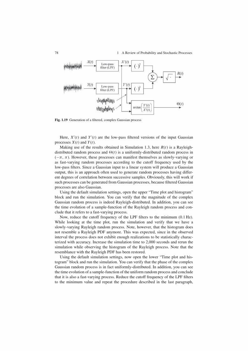
78 1 A Review of Probability and Stochastic Processes
Fig. 1.19 Generation of a filtered, complex Gaussian process
Here, X ′(t) and Y ′(t) are the low-pass filtered versions of the input Gaussian
processes X (t) and Y (t).
Making use of the results obtained in Simulation 1.3, here R(t) is a Rayleigh-
distributed random process and Θ(t) is a uniformly-distributed random process in
(−π , π ). However, these processes can manifest themselves as slowly-varying or
as fast-varying random processes according to the cutoff frequency used by the
low-pass filters. Since a Gaussian input to a linear system will produce a Gaussian
output, this is an approach often used to generate random processes having differ-
ent degrees of correlation between successive samples. Obviously, this will work if
such processes can be generated from Gaussian processes, because filtered Gaussian
processes are also Gaussian.
Using the default simulation settings, open the upper “Time plot and histogram”
block and run the simulation. You can verify that the magnitude of the complex
Gaussian random process is indeed Rayleigh-distributed. In addition, you can see
the time evolution of a sample-function of the Rayleigh random process and con-
clude that it refers to a fast-varying process.
Now, reduce the cutoff frequency of the LPF filters to the minimum (0.1 Hz).
While looking at the time plot, run the simulation and verify that we have a
slowly-varying Rayleigh random process. Note, however, that the histogram does
not resemble a Rayleigh PDF anymore. This was expected, since in the observed
interval the process does not exhibit enough realizations to be statistically charac-
terized with accuracy. Increase the simulation time to 2,000 seconds and rerun the
simulation while observing the histogram of the Rayleigh process. Note that the
resemblance with the Rayleigh PDF has been restored.
Using the default simulation settings, now open the lower “Time plot and his-
togram” block and run the simulation. You can verify that the phase of the complex
Gaussian random process is in fact uniformly-distributed. In addition, you can see
the time evolution of a sample-function of the uniform random process and conclude
that it is also a fast-varying process. Reduce the cutoff frequency of the LPF filters
to the minimum value and repeat the procedure described in the last paragraph,

1.14 Random Processes 79
just to confirm that the uniformly-distributed random process also keeps its original
distribution, no matter how fast it is.
In Chap. 3 we shall revisit the complex Gaussian random process as representa-
tive of the typical behavior of one of the most important channels used by modern
communication systems: the wireless channel.
Explore inside the individual blocks. Try to understand how they were imple-
mented. Create and investigate for yourself new situations and configurations of the
simulation parameters, especially for the filter’s cutoff frequencies, and try to reach
your own conclusions.
1.14.5 Thermal Noise Process
In the context of communications systems, the term noise can be associated to any
impairment, normally random, that affects system performance.
Among the different types of noise, thermal noise and impulse (or impulsive)
noise deserve especial attention. Thermal noise, often called Gaussian noise or
Johnson-Nyquist noise, is a random process generated by the agitation of the elec-
trons inside an electrical conductor due to thermal influence. Impulsive noise is a
normally high amplitude pulse noise caused by disturbances having abrupt changes
and short durations. For example, switching processes in a circuit may cause impul-
sive noise. The ignition system of vehicles can also induce impulsive noise in an
electronic circuit.
Thermal noise is present in all communication systems and, for this reason, we
shall give some details about it in what follows. Additionally, since thermal noise
is a Gaussian random process, from the central limit theorem and under certain
circumstances the sum of noises coming from many different sources, no matter
their individual distributions, can be approximated to a Gaussian noise.
It can be shown that the mean square value of the noise voltage VT N across the
terminals of the equivalent Thevenin circuit in Fig. 1.20 is given by [7, pp. 220–224;
5, p. 60]
E[
V 2T N
]
= 4kTBR volts2, (1.206)
where k = 1.38047 × 10⁻²⁷ joule/Kelvin (J/K) is the Boltzmann constant, T is the
absolute temperature in Kelvin, B is the measuring bandwidth in hertz (Hz) and R
is the resistance in ohms (Ω).
In the condition of maximum power transfer, the load connected to the terminals
of the circuit in Fig. 1.20 must have R ohms. In this case, the average noise power
delivered to this load will be
N =
(√
E[
V 2T N
]
/2)2
R=
(√4kTBR/2
)2
R= kTB watts. (1.207)

80 1 A Review of Probability and Stochastic Processes
Fig. 1.20 Thevenin equivalent circuit for thermal noise generation
Since the number of electrons in a conductor is very large and their motions are
random and independent, the central limit theorem leads us to the conclusion that
the thermal noise voltage is a zero-mean Gaussian random process.
1.14.5.1 Additive White Gaussian Noise (AWGN)
In communication systems, thermal noise acts by addition to the signal of interest.
In this sense we say that the noise is additive. Moreover, due to the variety of the
electrons motion speeds, ranging from very slow to very high values, the frequency
content of the thermal noise will be very high. This fact has led to the flat theoretical
model for the power spectral density of this noise, that is,
SW ( f ) =N0
2W/Hz,−∞ ≤ f ≤ ∞, (1.208)
where N0 = kTe is the noise power spectral density produced at the input of a
communication receiver circuit for which the equivalent noise temperature is Te.
The equivalent noise temperature is a circuit-dependent parameter defined as the
temperature that a resistor must be submitted in order to produce the power density
N0 when connected to a noiseless version of the circuit.
Due to the flat model for the power spectral density of the thermal noise we say
that it is a white noise. This is an allusion to the white color, since its spectrum
contains the spectrum of all colors. Then, putting together all terms we usually call
the thermal noise an additive white Gaussian noise (AWGN).
Since the autocorrelation function and the power spectral density form a Fourier
transform pair, we have
RW (τ ) = ℑ−1SW ( f ) =N0
2δ(τ ), (1.209)
where ℑ−1· is the inverse Fourier transform and δ(τ ) is the Dirac delta function.
The power spectral density (1.208) and the autocorrelation function (1.209) of
the AWG noise are plotted in Fig. 1.21.

1.14 Random Processes 81
Fig. 1.21 Power spectral density (a) and autocorrelation function (b) of the AWGN
Note that the AWGN is the ultimate process in terms of randomness, since its
samples collected ∆ seconds apart will produce completely uncorrelated random
variables for any value of ∆ > 0. Furthermore, note that the total average power of
the AWGN is infinite, since it corresponds to the area under SW ( f ). This means that
this model is unrealizable in practice. However, for most applications it suffices to
consider that the thermal noise is white in the overall bandwidth of the system under
consideration and zero outside. As a result, the total average noise power becomes
finite.
1.14.5.2 Equivalent Noise Bandwidth
The flat noise bandwidth does not apply to all band-limited systems. In other words,
even if we consider the noise flat within the system bandwidth, the system’s response
might not be flat in this range. To solve this problem it is usual to work with an equiv-
alent noise bandwidth, defined as the bandwidth of an ideal filter that produces the
same noise power produced by the filter that represents the actual system’s response.
The responses of these filters are illustrated in Fig. 1.22.
Fig. 1.22 Illustrating the concept of the equivalent noise bandwidth
Considering a white noise applied to the actual filter, the average noise power at
the output of this filter will be

82 1 A Review of Probability and Stochastic Processes
N1 =∫ ∞
−∞
N0
2|H ( f )|2d f = N0
∫ ∞
0
|H ( f )|2d f. (1.210)
With the same white noise applied to the ideal filter of bandwidth B, the average
noise power in its output will be
N2 =N0
2H 2(0)2B. (1.211)
Equating N1 and N2 given in (1.210) and (1.211), the system’s equivalent noise
bandwidth is finally given by
B =∫ ∞
0|H ( f )|2d f
H 2(0). (1.212)
1.15 Summary and Further Reading
In this chapter we studied some concepts about probability and random processes,
with focus on those topics which are more directly applicable to the study of digital
communication systems.
We dedicated about 75% of the chapter to random variables and about 25% to
stochastic processes, since most of the concepts related to random variables are
applicable with minor adequacies to random processes. In other words, if one has a
good understanding about random variables, the concepts can be easily applied to
random processes. For example, the statistics of a random process is in fact obtained
from the statistics of the random variables derived from the process.
Many references were already cited throughout the chapter, according to each
specific topic covered. In what follows we give a short overview about some of the
references listed at the end of the chapter, aiming at helping the reader to find some
complementary subject when needed.
The book by A. Papoulis [10] is one of the most complete references in what con-
cerns the formal treatment of probability and random processes, without focusing
in a specific application or area.
In the book by L. B. Koralov and Y. G. Sinai [6], basic material found in essen-
tially all good books on probability and stochastic processes are addressed, but we
think that the main contribution of the authors is to provide a complementary mate-
rial not usually covered in detail in most of the similar books.
For a condensed overview of the main topics on probability and random pro-
cesses applied to the design and analysis of communication systems we recommend
Chaps. 10 and 11 of the book by B. P. Lathi [8], Chaps. 1 to 4 of the book by M. B.
Pursley [14], Chap. of the book by J. G. Proakis [13] and Chap. 1 and Appendix 1
from the book by S. Haykin [5].
A fundamental analysis of random processes with applications in communica-
tions theory is given by B. P. Lathi in [7]. The book by P. Z. Peebles [11], though

1.16 Additional Problems 83
applicable to engineering in general, focuses on some typical applications in com-
munication systems analysis.
For a deep treatment of probability and stochastic processes applied to Electrical
and Computer Engineering we recommend the books by A. Leon-Garcia [9], H.
Stark and J. W. Woods [15] and R. D. Yates and D. J. Goodman [18].
1.16 Additional Problems
Several simulation-oriented problems were already proposed in the body of the sim-
ulation work plans throughout the chapter. Most of the following additional propo-
sitions are also based on simulation or are research-oriented, requiring some sort of
additional reading. A number of exercises involving conventional calculations can
be found in the references cited throughout the chapter.
1. Suppose that you want to create your own lottery, in which K integer numbers
are drawn at random from a total of N integer numbers ranging from 1 to N .
A player can make a bet with J numbers. In a first version of the lottery you
have determined that N = 6, K = 2 and J = 2 or 3. Solve the following
propositions: (a) Compute C , the number of combinations of 2 numbers in your
lottery. List the possible combinations. (b) Determine P2, the probability of a
player win by making a bet with 2 numbers. (c) Determine P3, the probability
of a player win by making a bet with 3 numbers. (d) From the results obtained
in “a” and “b”, determine an expression for PJ , the probability of a player win
by making a bet with J numbers. (e) Now assume that an official lottery has 60
numbers and that draws of 6 numbers are made. Compute P7, the probability of
a player win by making a bet with 7 numbers.
2. Implement a VisSim/Comm diagram to simulate a discrete memoryless source
emitting symbols from the alphabet s0, s1, s2, s3, s4, s5, s6, s7, with a priori
probabilities p0, p1, p2, p3, p4, p5, p6, p7 = 0.2, 0.28, 0.1, 0.09, 0.01, 0.02,
0.16, 0.14, respectively. Hint: use the inverse CDF method for random number
generation.
3. Let X i , i = 1, 2, . . . , n, be a set of independent and identically distributed
random variables with mean µX and variance σ 2X . Determine the variance of
the random variable Z defined by:
Z =1
√
nσ 2X
(
n∑
i=1
X i − nµX
)
4. Suppose that, for reliability improvement purposes, a given machine has n
on-board computers operating in parallel and on an independent fashion. The
machine will continue to operate if at least one of its computers is operating
properly. Considering that a computer fails with probability p, determine the
probability that the machine will fail.
84 1 A Review of Probability and Stochastic Processes
5. An electronic equipment has 326 components, each of them with a probability
of failure of 0.001. Determine the probability of five or more components in
failure, assuming that failures occur independently.
6. A die is thrown two times. Determine the probability of 3 dots in the second
throw, given that 2 dots were presented in the first throw.
7. Using VisSim/Comm, implement an experiment capable of simulating the
throwing of two dices and the computation of some unconditional and con-
ditional probabilities via the relative frequency definition of probability.
8. Using the moment theorem, compute the mean, the mean square value and vari-
ance of the random variable whose PDF is given by:
fX (x) =
2e−2x , x ≥ 0
0 , x < 0
9. The random variables X and Y have the joint PDF fXY (x, y) given below. a)
determine the marginal PDFs of X and of Y . b) Based on the result in “a”,
can we state that the random variables X and Y are independent? Justify your
answer.
fXY (x, y) =
λµe−(λx+µy), x ≥ 0, y ≥ 0
0, otherwise
10. Do some research and make a dissertation about two goodness-of-fit tests of
your choice.
11. Let a white noise process W (t) with power spectral density N0/2 W/Hz be
applied to an ideal low-pass filter with bandwidth B Hz and unitary magni-
tude response. (a) Determine and sketch SN ( f ), the PSD of the noise N (t) at
the output of the filter. (b) Determine and sketch RN (τ ), the autocorrelation
function of N (t). (c) Compute N , the average power of the noise at the output
of the filter.
12. A stationary Gaussian random process X (t) with mean 10 volts is applied to the
input of a linear time-invariant system whose impulse response h(t) is given
below. The output process Y (t) has variance ψ . (a) Determine E[Y (t)]. (b)
Write the PDF of Y (t).
h(t) =
et/0.2, 0 ≤ t ≤ 0.1 s
0, otherwise
13. The magnitude of the frequency response of an RC low-pass filter is:
|H ( f )| =1
√
1 + (2π fRC)2, with R = 500 Ω and C = 10 µF.

References 85
To the input of this filter is applied a random process Z (t) generated by filtering
a white Gaussian noise W (t) by an ideal low-pass filter of bandwidth 50 Hz and
unitary gain. The power spectral density of W (t) is 0.001 W/Hz. (a) Determine
the equivalent noise bandwidth of the RC filter. (b) Compute the average power
of the process at the output of the filter. (c) Sketch |U ( f )|, the magnitude of the
frequency response of an ideal low-pass filter capable of providing the same
average power computed in “b”, when excited by W (t).
14. Using VisSim/Comm, implement a simulation capable of demonstrating that
when a Gaussian random process is filtered, another Gaussian random process
is produced at the output of the filter.
15. Using VisSim/Comm, implement a simulation capable of demonstrating the
concept of equivalent noise bandwidth.
References
1. Chung, K. L. and Aitsahlia, F. Elementary Probability Theory with Stochastic Processes andan Introduction to Mathematical Finance. 4th Ed. New York, USA: Springer-Verlag, 2003.
2. Coates, R. F. W., Janacek, G. J. and Lever, K. V. Monte Carlo Simulation and Random NumberGeneration. IEEE J. Selected Areas in Comm., vol. 6, pp. 58–66, January 1988.
3. Gentle, J. E. Random Number Generation and Monte Carlo Methods. 2nd Ed. New York, USA:Springer Science and Business Media, Inc., 2003.
4. Graf, R. F. Modern Dictionary of Electronics, 7th Ed, USA: Newnes & Butterworth-Heineman,1999.
5. Haykin, S. Communication Systems. 3rd Ed. New York, USA: John Wiley and Sons, Inc.,1994.
6. Koralov, L. B. and Sinai, Y. G. Theory of Probability and Random Processes. 2nd Ed. Berlin,Heidelberg: Springer-Verlag, 2007.
7. Lathi, B. P. An Introduction to Random Signals and Communication Theory. USA: Interna-tional Textbook Company, 1968.
8. Lathi, B. P. Modern Digital and Analog Communication Systems. 3rd Ed. New York, USA:Oxford University Press, 1998.
9. Leon-Garcia, A. Probability, Statistics, and Random Processes for Electrical Engineering. 3rd
Ed. Upper Saddle River, NJ, USA: Prentice Hall, 2008.10. Papoulis, A. Probability, Random Variables, and Stochastic Processes. 3rd Ed. New York,
USA: McGraw Hill, 1991.11. Peebles, P. Z. Probability, Random Variables and Random Signal Principles. 2nd Ed. New
York, USA: McGraw Hill, 1987.12. Pham, H. (Editor). Springer Handbook of Engineering Statistics. London, UK: Springer-
Verlag, 2006.13. Proakis, J. G. Digital Communications. 3rd Ed. USA: McGraw Hill, Inc., 1995.14. Pursley, M. B. Introduction to Digital Communications. Upper Saddle River, New Jersey,
USA: Prentice-Hall, 2005.15. Stark, H. and Woods, J. W. Probability and Random Processes with Applications to Signal
Processing. 3rd Ed. Upper Saddle River, NJ, USA: Prentice Hall, 2002.16. Wikipedia – The Free Encyclopedia on line. Available at: http://en.wikipedia.org (last access
on June 2009).17. Weisstein, E. Wolfram MathWorld. Available at: http://mathworld.wolfram.com (last access
on June 2009).18. Yates, R. D. and Goodman, D. J. Probability and Stochastic Processes: A Friendly Introduction
for Electrical and Computer Engineers. 2nd Ed. USA: John Wiley & Sons, Inc, 2005.