chapter6 integerprogramming · 206 chapter6. integerprogramming 6.1...
TRANSCRIPT
Chapter 6
Integer Programming
Integer programming (IP) deals with solving linear models in which some or allthe variables are restricted to be integer. There are algorithms especially designedfor IP problems which basically find the optimal solution by solving a sequenceof linear programming (LP) problems.
The simplex algorithm studied in Chapter 2 is based on the fact that the feasi-ble region (the set of feasible solutions) of an LP problem is convex. This propertyplays a key role in the solution of linear models. In fact, the number of extremepoints of a convex set of solutions is finite, and we have shown that the optimalsolution is obtained in an extreme point. Therefore, even though the number ofsolutions is reduced when variables are restricted to be integer, IP problems areusually much more difficult to solve than LP problems because the set of feasiblesolutions is no longer convex.
According to the nature of the variables, we can distinguish three types of IPmodels.
• In mixed integer programming, only some of the variables are restricted tointeger values.
• In pure integer programming, all the variables are integers.
• In binary integer programming or 0-1 integer programming, all the variablesare binary (restricted to the values 0 or 1).
205
206 Chapter 6. Integer Programming
6.1 Some applications of integer programming
This section presents some illustrative examples of typical integer programmingproblems (IP problems) and binary programming problems (0-1 IP problems).
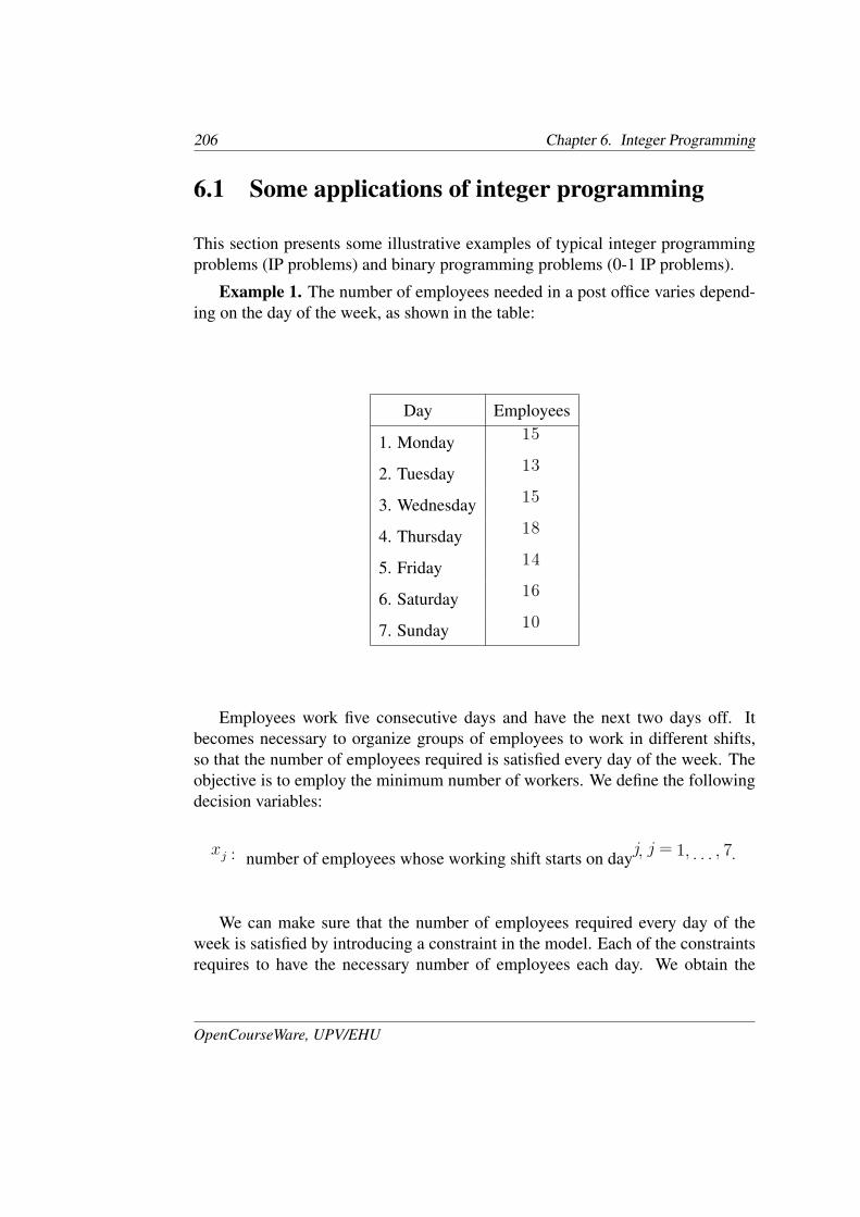
Example 1. The number of employees needed in a post office varies depend-ing on the day of the week, as shown in the table:
Day Employees
1. Monday 15
2. Tuesday 13
3. Wednesday 15
4. Thursday 18
5. Friday 14
6. Saturday 16
7. Sunday 10
Employees work five consecutive days and have the next two days off. Itbecomes necessary to organize groups of employees to work in different shifts,so that the number of employees required is satisfied every day of the week. Theobjective is to employ the minimum number of workers. We define the followingdecision variables:
xj : number of employees whose working shift starts on dayj, j = 1, . . . , 7.
We can make sure that the number of employees required every day of theweek is satisfied by introducing a constraint in the model. Each of the constraintsrequires to have the necessary number of employees each day. We obtain the
OpenCourseWare, UPV/EHU
6.1. Some applications of integer programming 207
following IP model:
min z = x1 + x2 + x3 + x4 + x5 + x6 + x7
subject tox1 + x4 + x5 + x6 + x7 ≥ 15
x1 + x2 + x5 + x6 + x7 ≥ 13
x1 + x2 + x3 + x6 + x7 ≥ 15
x1 + x2 + x3 + x4 + x7 ≥ 18
x1 + x2 + x3 + x4 + x5 ≥ 14
x2 + x3 + x4 + x5 + x6 ≥ 16
x3 + x4 + x5 + x6 + x7 ≥ 10
x1, x2, x3, x4, x5, x6, x7 ≥ 0 and integer
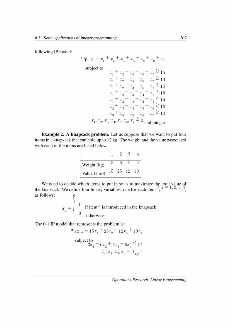
Example 2. A knapsack problem. Let us suppose that we want to put fouritems in a knapsack that can hold up to 12 kg. The weight and the value associatedwith each of the items are listed below:
1 2 3 4
Weight (kg) 3 6 5 5
Value (euro) 15 25 12 10
We need to decide which items to put in so as to maximize the total value ofthe knapsack. We define four binary variables, one for each item j, j = 1, 2, 3, 4,as follows:
xj =
1 if item j is introduced in the knapsack
0 otherwise
The 0-1 IP model that represents the problem is:
max z = 15x1 + 25x2 + 12x3 + 10x4
subject to3x1 + 6x2 + 5x3 + 5x4 ≤ 12
x1, x2, x3, x4 = 0 or 1
Operations Research. Linear Programming
208 Chapter 6. Integer Programming
We may also want to take into account other constraints in the problem, such asthe volume of the items.
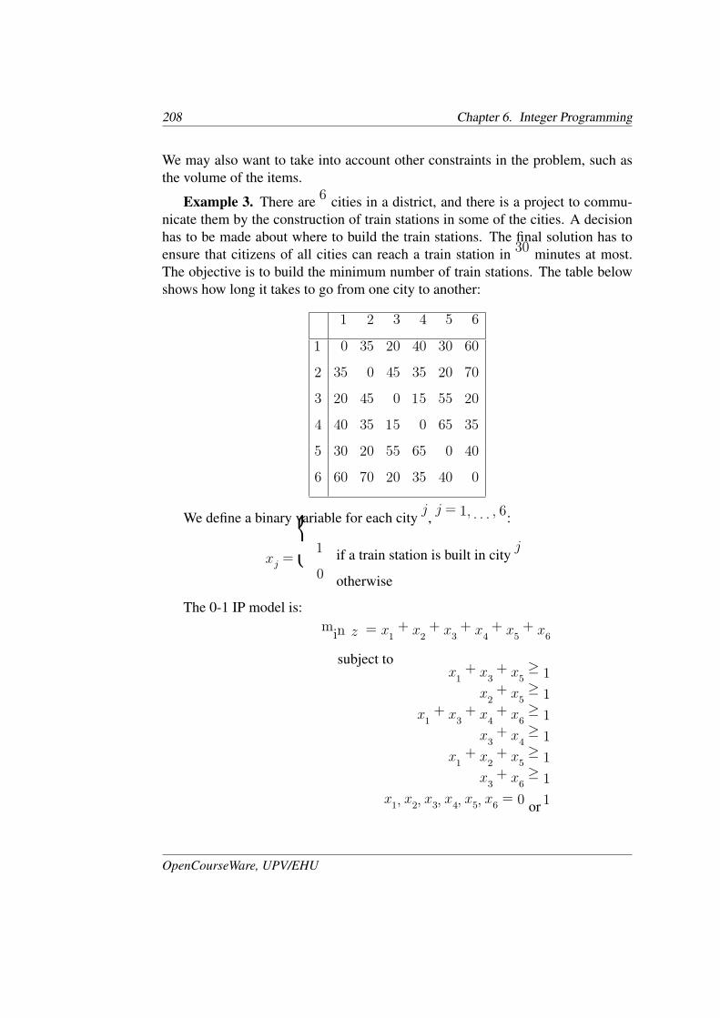
Example 3. There are 6 cities in a district, and there is a project to commu-nicate them by the construction of train stations in some of the cities. A decisionhas to be made about where to build the train stations. The final solution has toensure that citizens of all cities can reach a train station in 30 minutes at most.The objective is to build the minimum number of train stations. The table belowshows how long it takes to go from one city to another:
1 2 3 4 5 6
1 0 35 20 40 30 60
2 35 0 45 35 20 70
3 20 45 0 15 55 20
4 40 35 15 0 65 35
5 30 20 55 65 0 40
6 60 70 20 35 40 0
We define a binary variable for each city j, j = 1, . . . , 6:
xj =
1 if a train station is built in city j
0 otherwise
The 0-1 IP model is:
min z = x1 + x2 + x3 + x4 + x5 + x6
subject tox1 + x3 + x5 ≥ 1
x2 + x5 ≥ 1
x1 + x3 + x4 + x6 ≥ 1
x3 + x4 ≥ 1
x1 + x2 + x5 ≥ 1
x3 + x6 ≥ 1
x1, x2, x3, x4, x5, x6 = 0 or 1
OpenCourseWare, UPV/EHU
6.2. Solving integer programming problems 209
Each constraint refers to a city, and ensures that at least one train station willbe located no further than a 30 minute drive from each city.
6.2 Solving integer programming problemsIn this section we illustrate by means of an example the difficulties found whilesolving an IP problem.
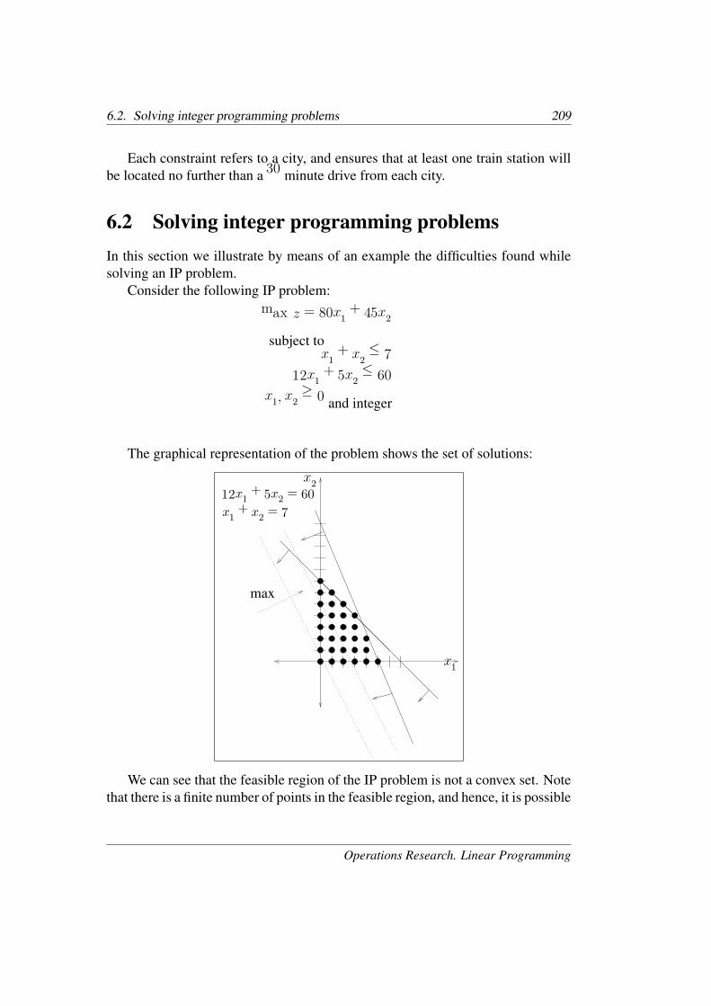
Consider the following IP problem:
max z = 80x1 + 45x2
subject tox1 + x2 ≤ 7
12x1 + 5x2 ≤ 60
x1, x2 ≥ 0 and integer
The graphical representation of the problem shows the set of solutions:
x1 + x2 = 7
12x1 + 5x2 = 60
x1
x2
max
We can see that the feasible region of the IP problem is not a convex set. Notethat there is a finite number of points in the feasible region, and hence, it is possible
Operations Research. Linear Programming
210 Chapter 6. Integer Programming
to find the optimal solution by computing the objective value z for each of thesolutions in the feasible region, and comparing them among each other. However,this method is not efficient for problems with a large number of variables, sincethe number of feasible points becomes extremely large.
In fact, a higher computational effort is required to solve an IP problem thanto solve the LP problem obtained by ignoring all integer constraints on variables,even though the number of feasible solutions to the IP problem is smaller. Thisis the case because contrary to LP problems, which have a convex set of feasiblesolutions, the feasible region of IP problems is not convex. Remind that the theorydeveloped in Chapter 2 is applicable whenever the set of solutions is convex.
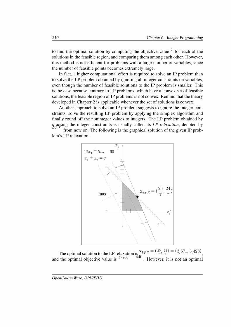
Another approach to solve an IP problem suggests to ignore the integer con-straints, solve the resulting LP problem by applying the simplex algorithm andfinally round off the noninteger values to integers. The LP problem obtained byignoring the integer constraints is usually called its LP relaxation, denoted byLPR from now on. The following is the graphical solution of the given IP prob-lem’s LP relaxation.
x1 + x2 = 7
12x1 + 5x2 = 60
x1
x2
xLPR = (25
7,24
7)max
The optimal solution to the LP relaxation is xLPR = (257, 24
7) = (3.571, 3.428),
and the optimal objective value is zLPR = 440. However, it is not an optimal
OpenCourseWare, UPV/EHU
6.3. The graphical solution of integer programming problems 211
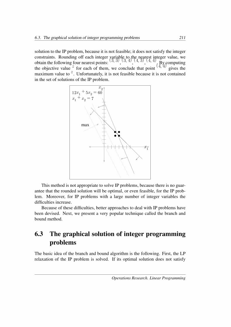
solution to the IP problem, because it is not feasible; it does not satisfy the integerconstraints. Rounding off each integer variable to the nearest integer value, weobtain the following four nearest points: (3, 3), (3, 4), (4, 3), (4, 4). By computingthe objective value z for each of them, we conclude that point (4, 4) gives themaximum value to z. Unfortunately, it is not feasible because it is not containedin the set of solutions of the IP problem.
x1 + x2 = 7
12x1 + 5x2 = 60
x1
x2
max
This method is not appropriate to solve IP problems, because there is no guar-antee that the rounded solution will be optimal, or even feasible, for the IP prob-lem. Moreover, for IP problems with a large number of integer variables thedifficulties increase.
Because of these difficulties, better approaches to deal with IP problems havebeen devised. Next, we present a very popular technique called the branch andbound method.
6.3 The graphical solution of integer programmingproblems
The basic idea of the branch and bound algorithm is the following. First, the LPrelaxation of the IP problem is solved. If its optimal solution does not satisfy
Operations Research. Linear Programming
212 Chapter 6. Integer Programming
the integer requirements, two additional LP problems are created by subdividingthe set of solutions of the LP relaxation. This partitioning is made in such away that a subset of noninteger solutions that contains the optimal solution to theLP relaxation is excluded from the set of solutions, and gives rise to the conceptof branching in the branch and bound algorithm. Afterwards, the two new LPproblems are solved.
In this section, we illustrate the branch and bound algorithm by applying it tothe IP problem shown on page 209. A sequence of LP relaxation problems areused to solve the IP problem, and their graphical solution represents the sets ofsolutions very appropriately. Let us consider the IP problem and its LP relaxation.
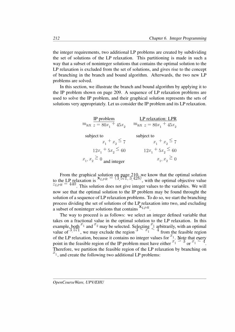
IP problem LP relaxation: LPR
max z = 80x1 + 45x2 max z = 80x1 + 45x2
subject to subject to
x1 + x2 ≤ 7 x1 + x2 ≤ 7
12x1 + 5x2 ≤ 60 12x1 + 5x2 ≤ 60
x1, x2 ≥ 0 and integer x1, x2 ≥ 0
From the graphical solution on page 210, we know that the optimal solutionto the LP relaxation is xLPR = (3.571, 3.428), with the optimal objective valuezLPR = 440. This solution does not give integer values to the variables. We willnow see that the optimal solution to the IP problem may be found throught thesolution of a sequence of LP relaxation problems. To do so, we start the branchingprocess dividing the set of solutions of the LP relaxation into two, and excludinga subset of noninteger solutions that contains xLPR.
The way to proceed is as follows: we select an integer defined variable thattakes on a fractional value in the optimal solution to the LP relaxation. In thisexample, both x1 and x2 may be selected. Selecting x1 arbitrarily, with an optimalvalue of 3.571, we may exclude the region 3 < x1 < 4 from the feasible regionof the LP relaxation, because it contains no integer values for x1. Note that everypoint in the feasible region of the IP problem must have either x1 ≤ 3 or x1 ≥ 4.Therefore, we partition the feasible region of the LP relaxation by branching onx1, and create the following two additional LP problems:
OpenCourseWare, UPV/EHU
6.3. The graphical solution of integer programming problems 213
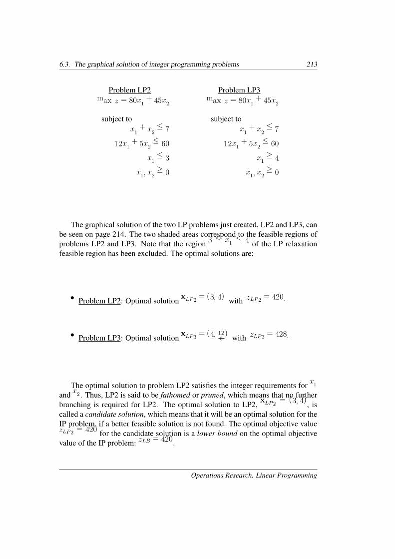
Problem LP2 Problem LP3
max z = 80x1 + 45x2 max z = 80x1 + 45x2
subject to subject to
x1 + x2 ≤ 7 x1 + x2 ≤ 7
12x1 + 5x2 ≤ 60 12x1 + 5x2 ≤ 60
x1 ≤ 3 x1 ≥ 4
x1, x2 ≥ 0 x1, x2 ≥ 0
The graphical solution of the two LP problems just created, LP2 and LP3, canbe seen on page 214. The two shaded areas correspond to the feasible regions ofproblems LP2 and LP3. Note that the region 3 < x1 < 4 of the LP relaxationfeasible region has been excluded. The optimal solutions are:
• Problem LP2: Optimal solution xLP2 = (3, 4) with zLP2 = 420.
• Problem LP3: Optimal solution xLP3 = (4, 125) with zLP3 = 428.
The optimal solution to problem LP2 satisfies the integer requirements for x1
and x2. Thus, LP2 is said to be fathomed or pruned, which means that no furtherbranching is required for LP2. The optimal solution to LP2, xLP2 = (3, 4), iscalled a candidate solution, which means that it will be an optimal solution for theIP problem, if a better feasible solution is not found. The optimal objective valuezLP2 = 420 for the candidate solution is a lower bound on the optimal objectivevalue of the IP problem: zLB = 420.
Operations Research. Linear Programming
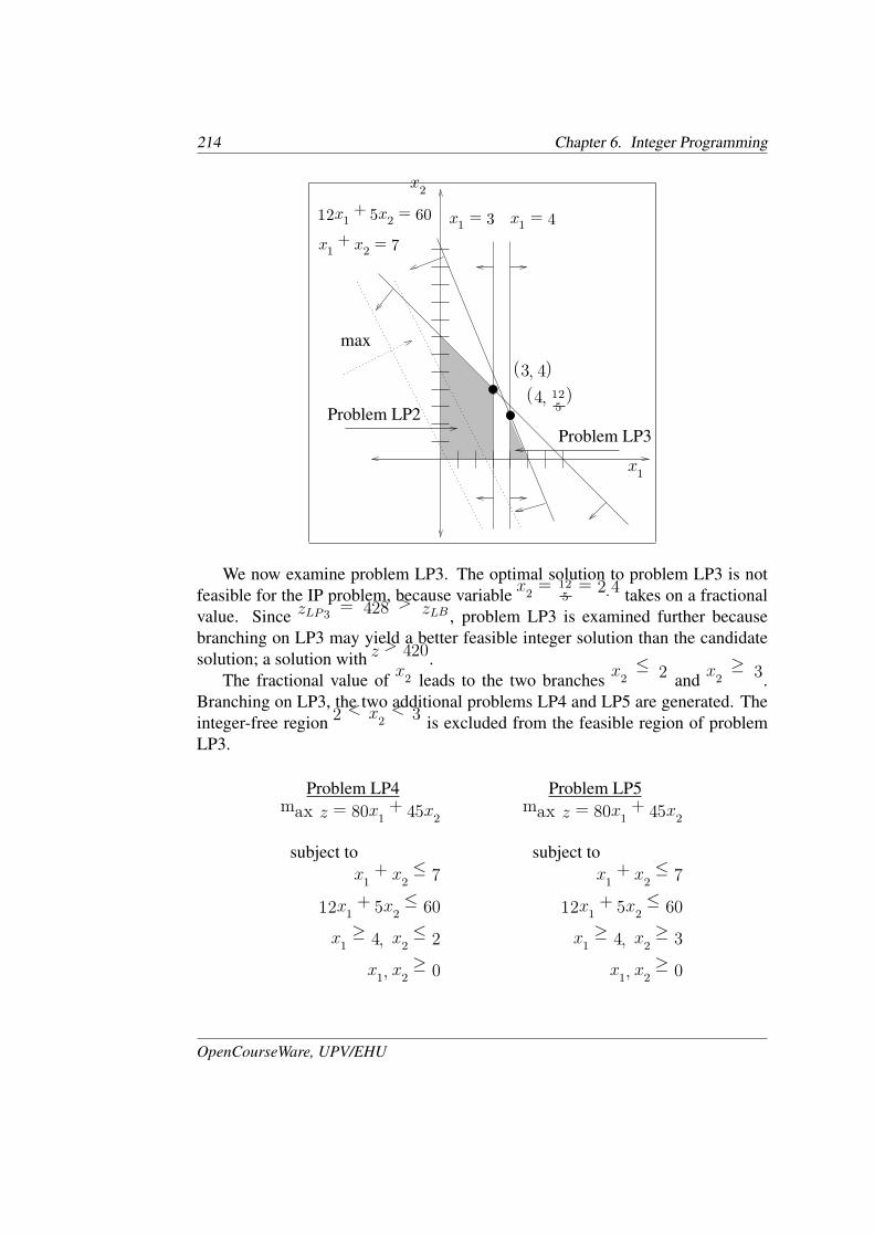
214 Chapter 6. Integer Programming
x1 + x2 = 7
12x1 + 5x2 = 60 x1 = 3 x1 = 4
x1
x2
(3, 4)
(4, 125)
max
Problem LP2Problem LP3
We now examine problem LP3. The optimal solution to problem LP3 is notfeasible for the IP problem, because variable x2 = 12
5= 2.4 takes on a fractional
value. Since zLP3 = 428 > zLB , problem LP3 is examined further becausebranching on LP3 may yield a better feasible integer solution than the candidatesolution; a solution with z > 420.
The fractional value of x2 leads to the two branches x2 ≤ 2 and x2 ≥ 3.Branching on LP3, the two additional problems LP4 and LP5 are generated. Theinteger-free region 2 < x2 < 3 is excluded from the feasible region of problemLP3.
Problem LP4 Problem LP5
max z = 80x1 + 45x2 max z = 80x1 + 45x2
subject to subject to
x1 + x2 ≤ 7 x1 + x2 ≤ 7
12x1 + 5x2 ≤ 60 12x1 + 5x2 ≤ 60
x1 ≥ 4, x2 ≤ 2 x1 ≥ 4, x2 ≥ 3
x1, x2 ≥ 0 x1, x2 ≥ 0
OpenCourseWare, UPV/EHU
6.3. The graphical solution of integer programming problems 215
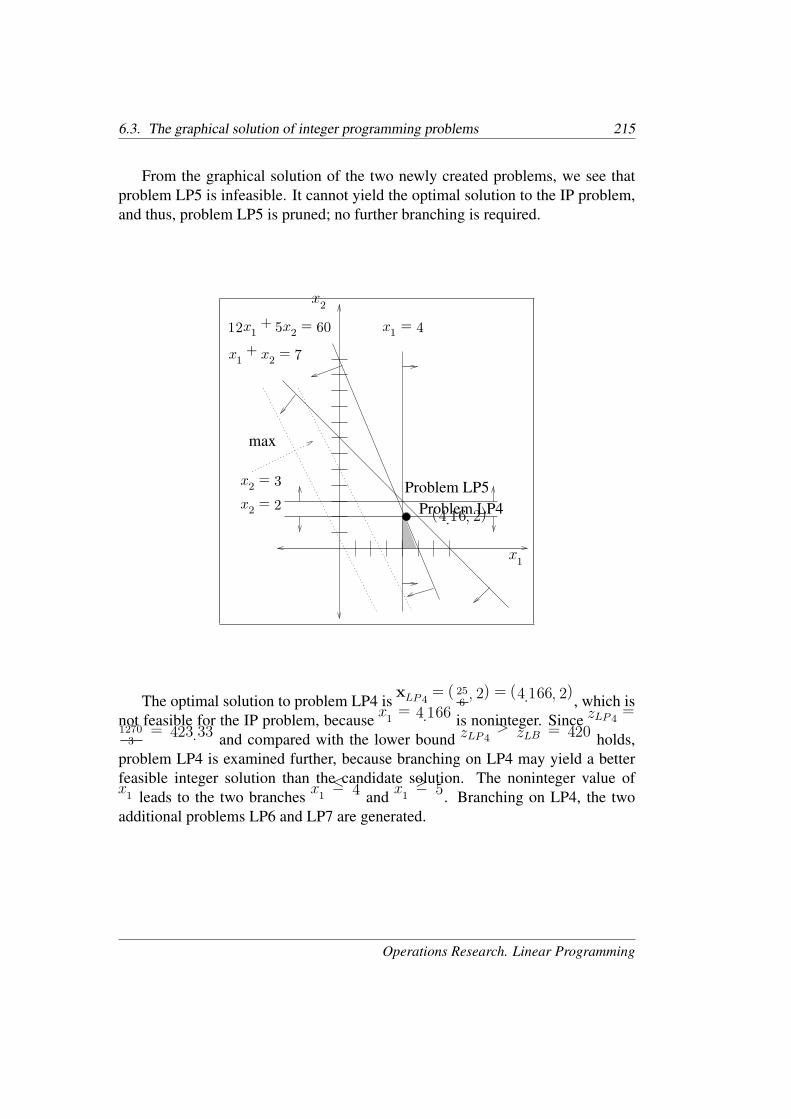
From the graphical solution of the two newly created problems, we see thatproblem LP5 is infeasible. It cannot yield the optimal solution to the IP problem,and thus, problem LP5 is pruned; no further branching is required.
x1 + x2 = 7
12x1 + 5x2 = 60 x1 = 4
x2 = 3
x2 = 2
x1
x2
(4.16, 2)
max
Problem LP4Problem LP5
The optimal solution to problem LP4 is xLP4 = (256, 2) = (4.166, 2), which is
not feasible for the IP problem, because x1 = 4.166 is noninteger. Since zLP4 =1270
3= 423.33 and compared with the lower bound zLP4 > zLB = 420 holds,
problem LP4 is examined further, because branching on LP4 may yield a betterfeasible integer solution than the candidate solution. The noninteger value ofx1 leads to the two branches x1 ≤ 4 and x1 ≥ 5. Branching on LP4, the twoadditional problems LP6 and LP7 are generated.
Operations Research. Linear Programming
216 Chapter 6. Integer Programming
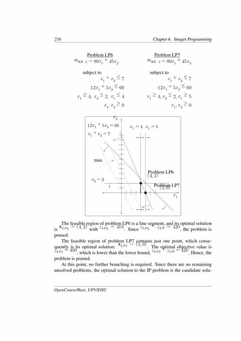
Problem LP6 Problem LP7
max z = 80x1 + 45x2 max z = 80x1 + 45x2
subject to subject to
x1 + x2 ≤ 7 x1 + x2 ≤ 7
12x1 + 5x2 ≤ 60 12x1 + 5x2 ≤ 60
x1 ≥ 4, x2 ≤ 2, x1 ≤ 4 x1 ≥ 4, x2 ≤ 2, x1 ≥ 5
x1, x2 ≥ 0 x1, x2 ≥ 0
x1 + x2 = 7
12x1 + 5x2 = 60 x1 = 4
x2 = 2
x1 = 5
x1
x2
(4, 2)
(5, 0)
max
Problem LP6
Problem LP7
The feasible region of problem LP6 is a line segment, and its optimal solutionis xLP6 = (4, 2) with zLP6 = 410. Since zLP6 < zLB = 420, the problem ispruned.
The feasible region of problem LP7 contains just one point, which conse-quently is its optimal solution: xLP7 = (5, 0). The optimal objective value iszLP7 = 400, which is lower than the lower bound, zLP7 < zLB = 420. Hence, theproblem is pruned.
At this point, no further branching is required. Since there are no remainingunsolved problems, the optimal solution to the IP problem is the candidate solu-
OpenCourseWare, UPV/EHU
6.4. The branch and bound method 217
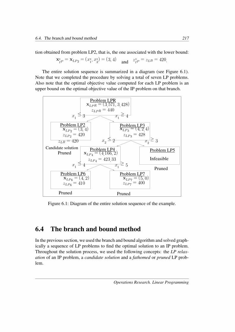
tion obtained from problem LP2, that is, the one associated with the lower bound:
x∗
IP = xLP2 = (x∗
1, x∗
2) = (3, 4) and z∗IP = zLB = 420.
The entire solution sequence is summarized in a diagram (see Figure 6.1).Note that we completed the procedure by solving a total of seven LP problems.Also note that the optimal objective value computed for each LP problem is anupper bound on the optimal objective value of the IP problem on that branch.
Problem LPR
Problem LP2 Problem LP3
Problem LP4 Problem LP5
Problem LP6 Problem LP7
xLPR = (3.571, 3.428)
xLP2 = (3, 4) xLP3 = (4, 2.4)
xLP4 = (4.166, 2)Infeasible
xLP6 = (4, 2) xLP7 = (5, 0)
zLPR = 440
zLP2 = 420 zLP3 = 428
zLP4 = 423.33
zLP6 = 410 zLP7 = 400
zLB = 420
x1 ≤ 3 x1 ≥ 4
x2 ≤ 2 x2 ≥ 3
x1 ≤ 4 x1 ≥ 5
Candidate solution
Pruned
PrunedPruned
Pruned
Figure 6.1: Diagram of the entire solution sequence of the example.
6.4 The branch and bound methodIn the previous section, we used the branch and bound algorithm and solved graph-ically a sequence of LP problems to find the optimal solution to an IP problem.Throughout the solution process, we used the following concepts: the LP relax-ation of an IP problem, a candidate solution and a fathomed or pruned LP prob-lem.
Operations Research. Linear Programming
218 Chapter 6. Integer Programming
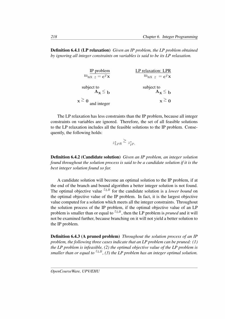
Definition 6.4.1 (LP relaxation) Given an IP problem, the LP problem obtainedby ignoring all integer constraints on variables is said to be its LP relaxation.
IP problem LP relaxation: LPR
max z = cTx max z = cTx
subject to subject to
Ax ≤ b Ax ≤ b
x ≥ 0 and integer x ≥ 0
The LP relaxation has less constraints than the IP problem, because all integerconstraints on variables are ignored. Therefore, the set of all feasible solutionsto the LP relaxation includes all the feasible solutions to the IP problem. Conse-quently, the following holds:
z∗LPR ≥ z∗IP .
Definition 6.4.2 (Candidate solution) Given an IP problem, an integer solutionfound throughout the solution process is said to be a candidate solution if it is thebest integer solution found so far.
A candidate solution will become an optimal solution to the IP problem, if atthe end of the branch and bound algorithm a better integer solution is not found.The optimal objective value zLB for the candidate solution is a lower bound onthe optimal objective value of the IP problem. In fact, it is the largest objectivevalue computed for a solution which meets all the integer constraints. Throughoutthe solution process of the IP problem, if the optimal objective value of an LPproblem is smaller than or equal to zLB , then the LP problem is pruned and it willnot be examined further, because branching on it will not yield a better solution tothe IP problem.
Definition 6.4.3 (A pruned problem) Throughout the solution process of an IPproblem, the following three cases indicate that an LP problem can be pruned: (1)the LP problem is infeasible, (2) the optimal objective value of the LP problem issmaller than or equal to zLB , (3) the LP problem has an integer optimal solution.
OpenCourseWare, UPV/EHU
6.4. The branch and bound method 219
For instance, problems LP2, LP5, LP6 and LP7 are pruned problems (seeFigure 6.1).
As it was previously said, the optimal objective value of an LP problem is anupper bound on the optimal objective value of the IP problem on that branch. Weuse the notation zUB to denote the upper bound that the optimal objective value ofeach LP problem establishes throughout the solution process of an IP problem.
6.4.1 The branch and bound algorithmLet us assume we have a maximization IP problem. The branch and bound algo-rithm can be summarized in the following steps:
* Step 1. InitializationSolve the LP relaxation associated with the IP problem to be solved.
– If the optimal solution to the LP relaxation satisfies the integer con-straints, then it is an optimal solution to the IP problem. Stop.
– Otherwise, set zLB = −∞ to initialize the lower bound on the optimalobjective value of the IP problem.
* Step 2. BranchingSelect an LP problem among the LP problems that can be branched out.Choose a variable xj which is integer-restricted in the IP problem but has anoninteger value in the optimal solution of the selected LP problem. Createtwo new LP problems adding the constraints1 xj ≤ [xj ] and xj ≥ [xj ] + 1to the LP problem.
* Step 3. BoundingSolve2 the two LP problems created in Step 2, and compute the objectivevalue zUB for each of them.
* Step 4. PruningAn LP problem may be pruned and therefore eliminated from further con-sideration, in the following cases:
(1) Pruned by infeasibility. The problem is infeasible.1[xj ] represents the greatest integer less than or equal to xj2Sensitivity analysis is commonly used and the dual simplex algorithm applied.
Operations Research. Linear Programming
220 Chapter 6. Integer Programming
(2) Pruned by bound. zUB ≤ zLB , that is, the optimal objective value ofthe LP problem is smaller than or equal to the lower bound.
(3) Pruned by optimality. The optimal solution is integer and zUB > zLB .Change the lower bound to the new value, zLB =zUB; the solutionassociated with the new lower bound is the new candidate solution.
If there are LP problems that can be branched out, then go to Step 2, andperform another iteration. Otherwise, the candidate solution is the optimalsolution to the IP problem. If no candidate solution has been found, the IPproblem is infeasible.
Even though a high computational effort is required to find the optimal solu-tion to an IP problem by applying the branch and bound algorithm, it is the mostpopular algorithm used to solve both mixed and pure IP problems.
Note that Step 2 is quite flexible, because it does not specify neither how toselect an LP problem to be branched out nor how to choose a branching variablexj , if there are several choices. Several rules have been designed to avoid arbi-trary choices and guide the search of an optimal solution to the IP problem. Infact, experience has shown that the way such decisions are made has an importanteffect on the computational efficiency of the branch and bound algorithm. A com-monly used rule to select an LP problem to be branched out is the best bound rule,which suggests that the LP problem with the largest upper bound zUB should beselected. Some rules have also been designed to choose a branching variable, butunfortunately, they are quite complex. In the following example, we choose thebranching variable arbitrarily.
Example. We apply the branch and bound algorithm to find the optimal solu-tion to the IP problem shown on page 209.
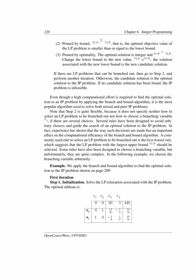
First iterationStep 1. Initialization. Solve the LP relaxation associated with the IP problem.
The optimal tableau is:
x1 x2 x3 x4
0 0 20 5 440
a2 0 1 12
7−1
7
24
7
a1 1 0 −5
7
1
7
25
7
OpenCourseWare, UPV/EHU
6.4. The branch and bound method 221
Set zLB = −∞ to initialize the lower bound.Step 2. Branching. The optimal solution to the LP relaxation is not integer.
We choose the branching variable, x1 for instance, and create two new problems:problem LP2 and problem LP3 (see page 212).
Step 3. Bounding. We solve the two LP problems created in Step 2 using thesensitivity analysis and the dual simplex algorithm.
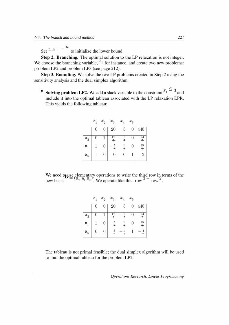
• Solving problem LP2. We add a slack variable to the constraint x1 ≤ 3 andinclude it into the optimal tableau associated with the LP relaxation LPR.This yields the following tableau:
x1 x2 x3 x4 x5
0 0 20 5 0 440
a2 0 1 12
7−1
70 24
7
a1 1 0 −5
7
1
70 25
7
a5 1 0 0 0 1 3
We need to use elementary operations to write the third row in terms of thenew basis B = (a2 a1 a5). We operate like this: row 3 − row 2.
x1 x2 x3 x4 x5
0 0 20 5 0 440
a2 0 1 12
7−1
70 24
7
a1 1 0 −5
7
1
70 25
7
a5 0 0 5
7−1
71 −4
7
The tableau is not primal feasible; the dual simplex algorithm will be usedto find the optimal tableau for the problem LP2.
Operations Research. Linear Programming
222 Chapter 6. Integer Programming
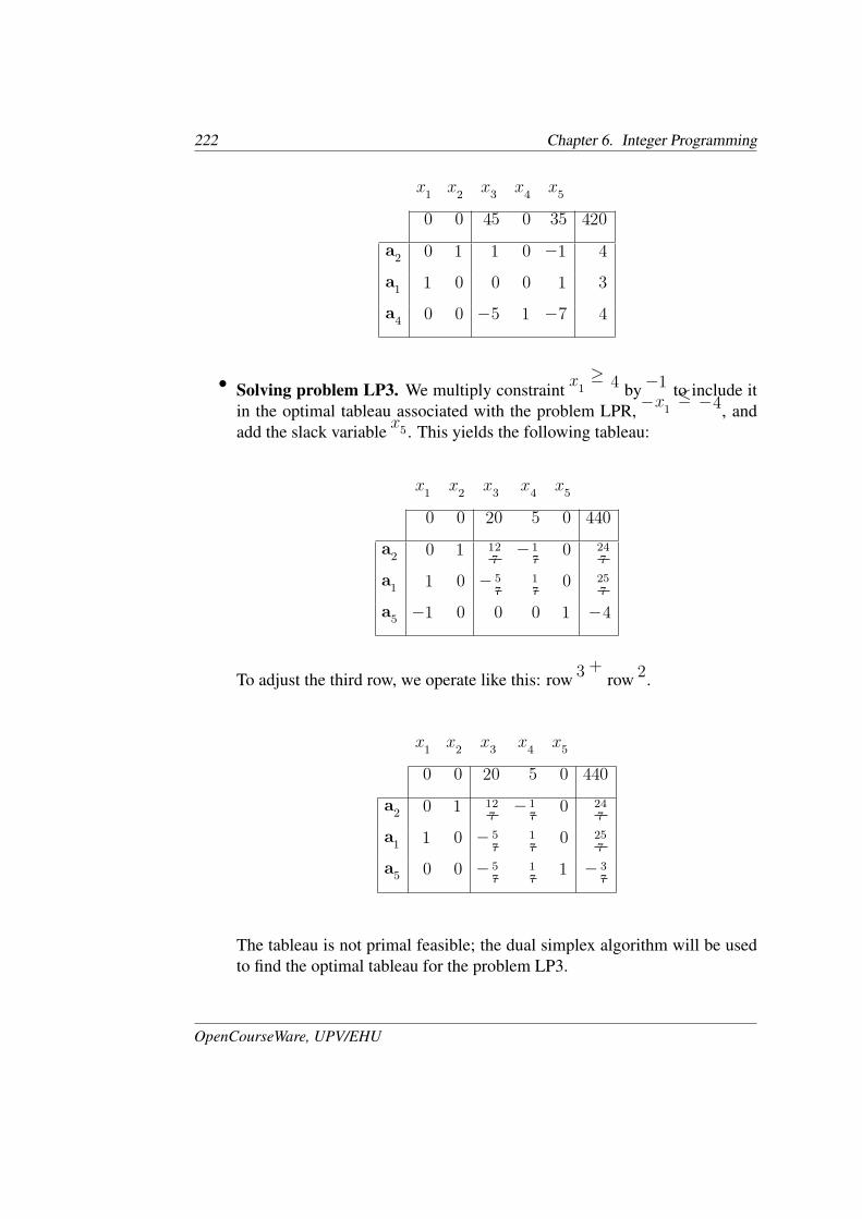
x1 x2 x3 x4 x5
0 0 45 0 35 420
a2 0 1 1 0 −1 4
a1 1 0 0 0 1 3
a4 0 0 −5 1 −7 4
• Solving problem LP3. We multiply constraint x1 ≥ 4 by −1 to include itin the optimal tableau associated with the problem LPR, −x1 ≤ −4, andadd the slack variable x5. This yields the following tableau:
x1 x2 x3 x4 x5
0 0 20 5 0 440
a2 0 1 12
7−1
70 24
7
a1 1 0 −5
7
1
70 25
7
a5 −1 0 0 0 1 −4
To adjust the third row, we operate like this: row 3 + row 2.
x1 x2 x3 x4 x5
0 0 20 5 0 440
a2 0 1 12
7−1
70 24
7
a1 1 0 −5
7
1
70 25
7
a5 0 0 −5
7
1
71 −3
7
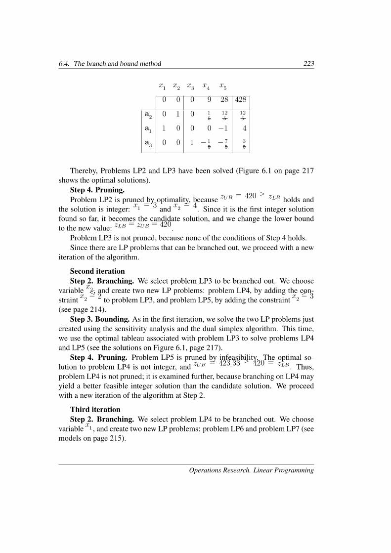
The tableau is not primal feasible; the dual simplex algorithm will be usedto find the optimal tableau for the problem LP3.
OpenCourseWare, UPV/EHU
6.4. The branch and bound method 223
x1 x2 x3 x4 x5
0 0 0 9 28 428
a2 0 1 0 1
5
12
5
12
5
a1 1 0 0 0 −1 4
a3 0 0 1 −1
5−7
5
3
5
Thereby, Problems LP2 and LP3 have been solved (Figure 6.1 on page 217shows the optimal solutions).
Step 4. Pruning.Problem LP2 is pruned by optimality, because zUB = 420 > zLB holds and
the solution is integer: x1 = 3 and x2 = 4. Since it is the first integer solutionfound so far, it becomes the candidate solution, and we change the lower boundto the new value: zLB = zUB = 420.
Problem LP3 is not pruned, because none of the conditions of Step 4 holds.Since there are LP problems that can be branched out, we proceed with a new
iteration of the algorithm.
Second iterationStep 2. Branching. We select problem LP3 to be branched out. We choose
variable x2, and create two new LP problems: problem LP4, by adding the con-straint x2 ≤ 2 to problem LP3, and problem LP5, by adding the constraint x2 ≥ 3(see page 214).
Step 3. Bounding. As in the first iteration, we solve the two LP problems justcreated using the sensitivity analysis and the dual simplex algorithm. This time,we use the optimal tableau associated with problem LP3 to solve problems LP4and LP5 (see the solutions on Figure 6.1, page 217).
Step 4. Pruning. Problem LP5 is pruned by infeasibility. The optimal so-lution to problem LP4 is not integer, and zUB = 423.33 > 420 = zLB . Thus,problem LP4 is not pruned; it is examined further, because branching on LP4 mayyield a better feasible integer solution than the candidate solution. We proceedwith a new iteration of the algorithm at Step 2.
Third iterationStep 2. Branching. We select problem LP4 to be branched out. We choose
variable x1, and create two new LP problems: problem LP6 and problem LP7 (seemodels on page 215).
Operations Research. Linear Programming
224 Chapter 6. Integer Programming
Step 3. Bounding. We solve the two LP problems just created. This time,we start from the optimal tableau associated with problem LP4 to solve problemsLP6 and LP7 (see the solutions on Figure 6.1, page 217).
Step 4. Pruning.Problem LP6 is pruned by bound, because zUB = 410 < 420 = zLB holds.Problem LP7 is also pruned by bound, since zUB = 400 < 420 = zLB holds.No problem remains to be branched out. Therefore, the candidate solution is
the optimal solution to the IP problem.
x∗
1 = 3, x∗
2 = 4, z∗IP = zLB = 420.
�
6.5 0-1 integer programmingIn practice, there are problems where all the variables are binary, and for the solu-tion of which different algorithms have been proposed. In this section, we presentone which has basically the same structure as the branch and bound algorithmintroduced earlier.
Before we apply the algorithm to solve a 0-1 IP problem, we need to makesure that the coefficients of the objective function satisfy the following:
0 ≤ c1 ≤ c2 ≤ · · · ≤ cn (6.1)
It is always possible to rewrite the 0-1 IP model and obtain a form that satisfiesthe condition (6.1). Let us see how to proceed by means of an example.
Example. Consider the following 0-1 IP model:
max z = 6x1 − 4x2
subject to3x1 + 2x2 ≤ 10
−x1 + x2 ≤ 17
x1, x2 = 0 or 1
Cost coefficients in the objective function do not satisfy the condition (6.1). Toobtain the required form, we proceed like this: we consider the absolute value of
OpenCourseWare, UPV/EHU
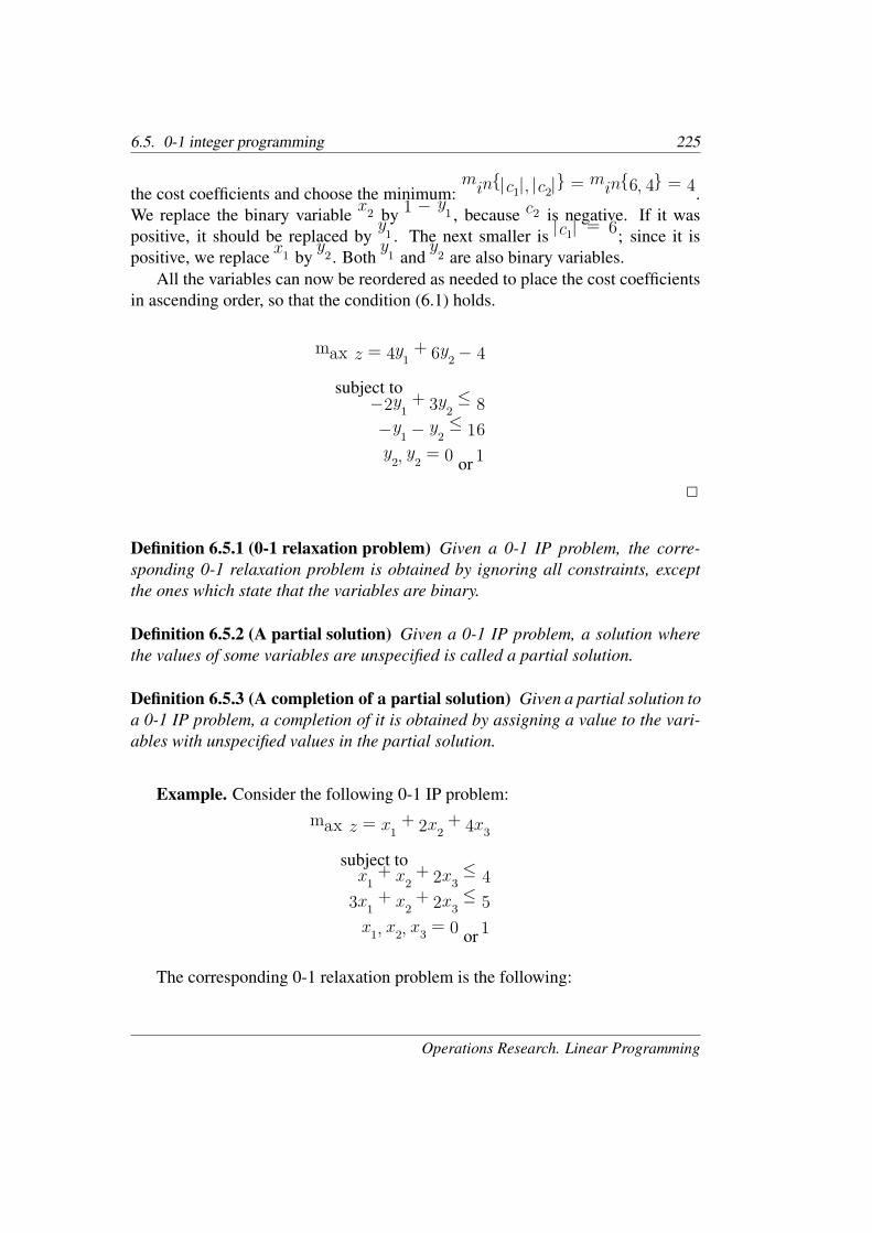
6.5. 0-1 integer programming 225
the cost coefficients and choose the minimum: min{|c1|, |c2|} = min{6, 4} = 4.We replace the binary variable x2 by 1 − y1, because c2 is negative. If it waspositive, it should be replaced by y1. The next smaller is |c1| = 6; since it ispositive, we replace x1 by y2. Both y1 and y2 are also binary variables.
All the variables can now be reordered as needed to place the cost coefficientsin ascending order, so that the condition (6.1) holds.
max z = 4y1 + 6y2 − 4
subject to−2y1 + 3y2 ≤ 8
−y1 − y2 ≤ 16
y2, y2 = 0 or 1
�
Definition 6.5.1 (0-1 relaxation problem) Given a 0-1 IP problem, the corre-sponding 0-1 relaxation problem is obtained by ignoring all constraints, exceptthe ones which state that the variables are binary.
Definition 6.5.2 (A partial solution) Given a 0-1 IP problem, a solution wherethe values of some variables are unspecified is called a partial solution.
Definition 6.5.3 (A completion of a partial solution) Given a partial solution toa 0-1 IP problem, a completion of it is obtained by assigning a value to the vari-ables with unspecified values in the partial solution.
Example. Consider the following 0-1 IP problem:
max z = x1 + 2x2 + 4x3
subject tox1 + x2 + 2x3 ≤ 4
3x1 + x2 + 2x3 ≤ 5
x1, x2, x3 = 0 or 1
The corresponding 0-1 relaxation problem is the following:
Operations Research. Linear Programming
226 Chapter 6. Integer Programming
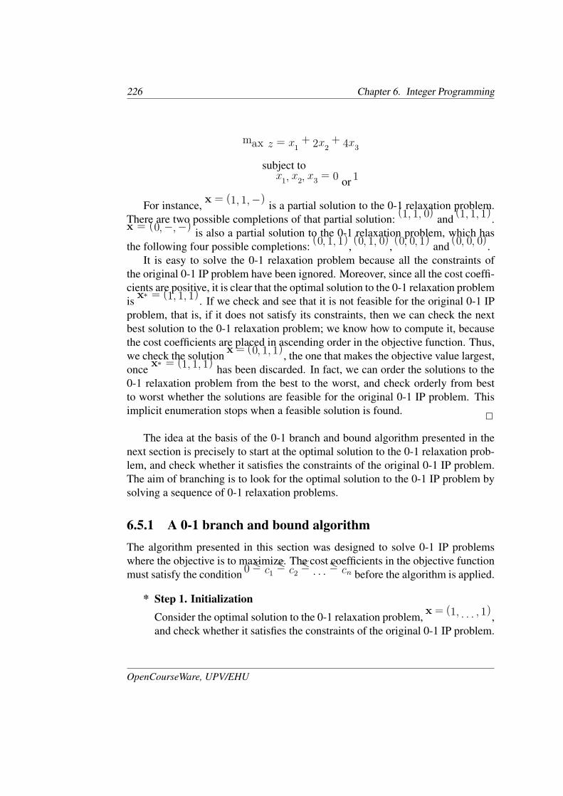
max z = x1 + 2x2 + 4x3
subject tox1, x2, x3 = 0 or 1
For instance, x = (1, 1,−) is a partial solution to the 0-1 relaxation problem.There are two possible completions of that partial solution: (1, 1, 0) and (1, 1, 1).x = (0,−,−) is also a partial solution to the 0-1 relaxation problem, which hasthe following four possible completions: (0, 1, 1), (0, 1, 0), (0, 0, 1) and (0, 0, 0).
It is easy to solve the 0-1 relaxation problem because all the constraints ofthe original 0-1 IP problem have been ignored. Moreover, since all the cost coeffi-cients are positive, it is clear that the optimal solution to the 0-1 relaxation problemis x∗ = (1, 1, 1). If we check and see that it is not feasible for the original 0-1 IPproblem, that is, if it does not satisfy its constraints, then we can check the nextbest solution to the 0-1 relaxation problem; we know how to compute it, becausethe cost coefficients are placed in ascending order in the objective function. Thus,we check the solution x = (0, 1, 1), the one that makes the objective value largest,once x∗ = (1, 1, 1) has been discarded. In fact, we can order the solutions to the0-1 relaxation problem from the best to the worst, and check orderly from bestto worst whether the solutions are feasible for the original 0-1 IP problem. Thisimplicit enumeration stops when a feasible solution is found.
�
The idea at the basis of the 0-1 branch and bound algorithm presented in thenext section is precisely to start at the optimal solution to the 0-1 relaxation prob-lem, and check whether it satisfies the constraints of the original 0-1 IP problem.The aim of branching is to look for the optimal solution to the 0-1 IP problem bysolving a sequence of 0-1 relaxation problems.
6.5.1 A 0-1 branch and bound algorithmThe algorithm presented in this section was designed to solve 0-1 IP problemswhere the objective is to maximize. The cost coefficients in the objective functionmust satisfy the condition 0 ≤ c1 ≤ c2 ≤ · · · ≤ cn before the algorithm is applied.
* Step 1. InitializationConsider the optimal solution to the 0-1 relaxation problem, x = (1, . . . , 1),and check whether it satisfies the constraints of the original 0-1 IP problem.
OpenCourseWare, UPV/EHU
6.5. 0-1 integer programming 227
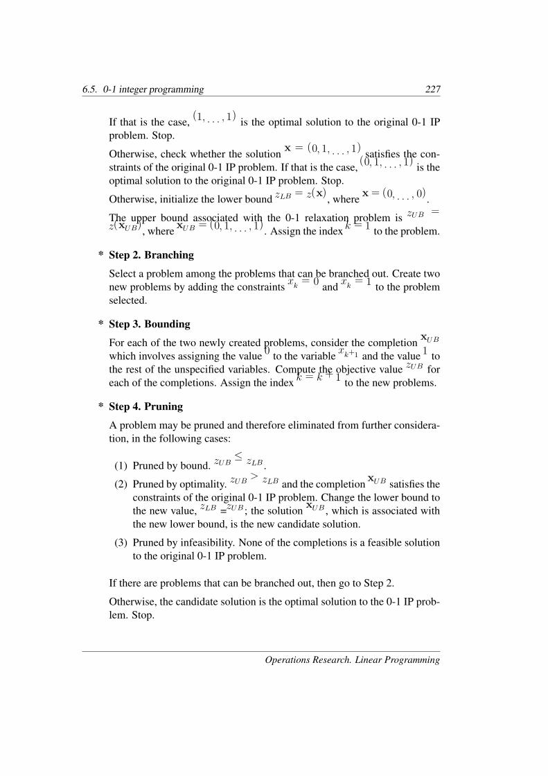
If that is the case, (1, . . . , 1) is the optimal solution to the original 0-1 IPproblem. Stop.
Otherwise, check whether the solution x = (0, 1, . . . , 1) satisfies the con-straints of the original 0-1 IP problem. If that is the case, (0, 1, . . . , 1) is theoptimal solution to the original 0-1 IP problem. Stop.
Otherwise, initialize the lower bound zLB = z(x), where x = (0, . . . , 0).
The upper bound associated with the 0-1 relaxation problem is zUB =z(xUB), where xUB = (0, 1, . . . , 1). Assign the index k = 1 to the problem.
* Step 2. Branching
Select a problem among the problems that can be branched out. Create twonew problems by adding the constraints xk = 0 and xk = 1 to the problemselected.
* Step 3. Bounding
For each of the two newly created problems, consider the completion xUB
which involves assigning the value 0 to the variable xk+1 and the value 1 tothe rest of the unspecified variables. Compute the objective value zUB foreach of the completions. Assign the index k = k + 1 to the new problems.
* Step 4. Pruning
A problem may be pruned and therefore eliminated from further considera-tion, in the following cases:
(1) Pruned by bound. zUB ≤ zLB .
(2) Pruned by optimality. zUB > zLB and the completion xUB satisfies theconstraints of the original 0-1 IP problem. Change the lower bound tothe new value, zLB =zUB; the solution xUB, which is associated withthe new lower bound, is the new candidate solution.
(3) Pruned by infeasibility. None of the completions is a feasible solutionto the original 0-1 IP problem.
If there are problems that can be branched out, then go to Step 2.
Otherwise, the candidate solution is the optimal solution to the 0-1 IP prob-lem. Stop.
Operations Research. Linear Programming
228 Chapter 6. Integer Programming
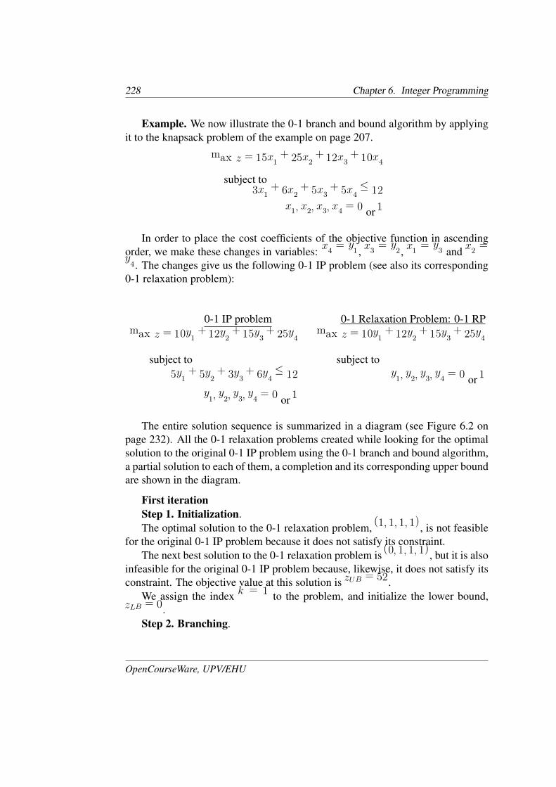
Example. We now illustrate the 0-1 branch and bound algorithm by applyingit to the knapsack problem of the example on page 207.
max z = 15x1 + 25x2 + 12x3 + 10x4
subject to3x1 + 6x2 + 5x3 + 5x4 ≤ 12
x1, x2, x3, x4 = 0 or 1
In order to place the cost coefficients of the objective function in ascendingorder, we make these changes in variables: x4 = y1, x3 = y2, x1 = y3 and x2 =y4. The changes give us the following 0-1 IP problem (see also its corresponding0-1 relaxation problem):
0-1 IP problem 0-1 Relaxation Problem: 0-1 RP
max z = 10y1 + 12y2 + 15y3 + 25y4 max z = 10y1 + 12y2 + 15y3 + 25y4
subject to subject to
5y1 + 5y2 + 3y3 + 6y4 ≤ 12 y1, y2, y3, y4 = 0 or 1
y1, y2, y3, y4 = 0 or 1
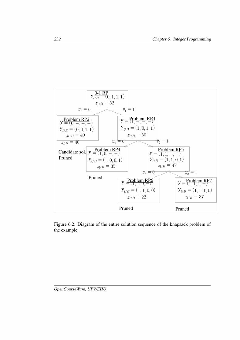
The entire solution sequence is summarized in a diagram (see Figure 6.2 onpage 232). All the 0-1 relaxation problems created while looking for the optimalsolution to the original 0-1 IP problem using the 0-1 branch and bound algorithm,a partial solution to each of them, a completion and its corresponding upper boundare shown in the diagram.
First iterationStep 1. Initialization.The optimal solution to the 0-1 relaxation problem, (1, 1, 1, 1), is not feasible
for the original 0-1 IP problem because it does not satisfy its constraint.The next best solution to the 0-1 relaxation problem is (0, 1, 1, 1), but it is also
infeasible for the original 0-1 IP problem because, likewise, it does not satisfy itsconstraint. The objective value at this solution is zUB = 52.
We assign the index k = 1 to the problem, and initialize the lower bound,zLB = 0.
Step 2. Branching.
OpenCourseWare, UPV/EHU
6.5. 0-1 integer programming 229
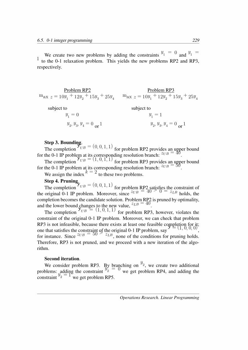
We create two new problems by adding the constraints y1 = 0 and y1 =1 to the 0-1 relaxation problem. This yields the new problems RP2 and RP3,respectively.
Problem RP2 Problem RP3
max z = 10y1 + 12y2 + 15y3 + 25y4 max z = 10y1 + 12y2 + 15y3 + 25y4
subject to subject to
y1 = 0 y1 = 1
y2, y3, y4 = 0 or 1 y2, y3, y4 = 0 or 1
Step 3. Bounding.The completion yUB = (0, 0, 1, 1) for problem RP2 provides an upper bound
for the 0-1 IP problem at its corresponding resolution branch: zUB = 40.The completion yUB = (1, 0, 1, 1) for problem RP3 provides an upper bound
for the 0-1 IP problem at its corresponding resolution branch: zUB = 50.We assign the index k = 2 to these two problems.Step 4. Pruning.The completion yUB = (0, 0, 1, 1) for problem RP2 satisfies the constraint of
the original 0-1 IP problem. Moreover, since zUB = 40 > 0 = zLB holds, thecompletion becomes the candidate solution. Problem RP2 is pruned by optimality,and the lower bound changes to the new value, zLB = 40.
The completion yUB = (1, 0, 1, 1) for problem RP3, however, violates theconstraint of the original 0-1 IP problem. Moreover, we can check that problemRP3 is not infeasible, because there exists at least one feasible completion for it;one that satisfies the constraint of the original 0-1 IP problem, say y = (1, 0, 0, 0),for instance. Since zUB = 50 > zLB , none of the conditions for pruning holds.Therefore, RP3 is not pruned, and we proceed with a new iteration of the algo-rithm.
Second iteration.We consider problem RP3. By branching on y2, we create two additional
problems: adding the constraint y2 = 0 we get problem RP4, and adding theconstraint y2 = 1 we get problem RP5.
Operations Research. Linear Programming
230 Chapter 6. Integer Programming
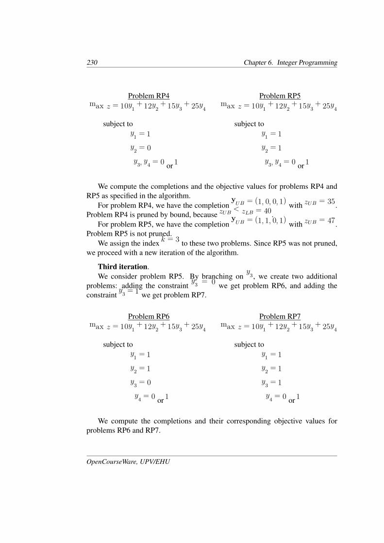
Problem RP4 Problem RP5
max z = 10y1 + 12y2 + 15y3 + 25y4 max z = 10y1 + 12y2 + 15y3 + 25y4
subject to subject to
y1 = 1 y1 = 1
y2 = 0 y2 = 1
y3, y4 = 0 or 1 y3, y4 = 0 or 1
We compute the completions and the objective values for problems RP4 andRP5 as specified in the algorithm.
For problem RP4, we have the completion yUB = (1, 0, 0, 1) with zUB = 35.Problem RP4 is pruned by bound, because zUB < zLB = 40.
For problem RP5, we have the completion yUB = (1, 1, 0, 1) with zUB = 47.Problem RP5 is not pruned.
We assign the index k = 3 to these two problems. Since RP5 was not pruned,we proceed with a new iteration of the algorithm.
Third iteration.We consider problem RP5. By branching on y3, we create two additional
problems: adding the constraint y3 = 0 we get problem RP6, and adding theconstraint y3 = 1 we get problem RP7.
Problem RP6 Problem RP7
max z = 10y1 + 12y2 + 15y3 + 25y4 max z = 10y1 + 12y2 + 15y3 + 25y4
subject to subject to
y1 = 1 y1 = 1
y2 = 1 y2 = 1
y3 = 0 y3 = 1
y4 = 0 or 1 y4 = 0 or 1
We compute the completions and their corresponding objective values forproblems RP6 and RP7.
OpenCourseWare, UPV/EHU
6.5. 0-1 integer programming 231
For problem RP6, we have the completion yUB = (1, 1, 0, 0) with zUB = 22.Problem RP6 is pruned by bound, because zUB < zLB = 40.
For problem RP7, we have the completion yUB = (1, 1, 1, 0) with zUB = 37.Problem RP7 is pruned by bound, because zUB < zLB = 40.
We assign the index k = 4 to these two problems.The 0-1 branch and bound algorithm stops, because there is no problem to be
branched out. Therefore, the solution associated with the lower bound zLB = 40,that is to say, the candidate solution, is the optimal solution to the 0-1 IP problem:yUB = (0, 0, 1, 1).
Undoing the change of variables, we obtain the optimal solution to the knap-sack problem of the example:
x∗
1 = 1, x∗
2 = 1, x∗
3 = 0, x∗
4 = 0, z∗ = 40.
Figure 6.2 summarizes the entire solution sequence in a diagram.�
Operations Research. Linear Programming
232 Chapter 6. Integer Programming
0-1 RP
Problem RP2 Problem RP3
Problem RP4 Problem RP5
Problem RP6 Problem RP7
y = (0,−,−,−) y = (1,−,−,−)
y = (1, 0,−,−) y = (1, 1,−,−)
y = (1, 1, 0,−) y = (1, 1, 1,−)
yUB = (0, 1, 1, 1)
yUB = (0, 0, 1, 1) yUB = (1, 0, 1, 1)
yUB = (1, 0, 0, 1) yUB = (1, 1, 0, 1)
yUB = (1, 1, 0, 0) yUB = (1, 1, 1, 0)
zUB = 52
zUB = 40 zUB = 50
zUB = 35 zUB = 47
zUB = 22 zUB = 37
zLB = 40
y1 = 0 y1 = 1
y2 = 0 y2 = 1
y3 = 0 y3 = 1
PrunedPruned
Pruned
PrunedCandidate sol.
Figure 6.2: Diagram of the entire solution sequence of the knapsack problem ofthe example.
OpenCourseWare, UPV/EHU