chapter8 reed-solomonand bose-chaudhuri-hocquenghem codes · 2010-08-03 · 280 8. reed-solomon...
TRANSCRIPT

Chapter 8
Reed-Solomon andBose-Chaudhuri-HocquenghemCodes
Several classes of codes were discussed in the previous chapters, including Ham-ming codes and the related dual simplex codes, repetition codes and the relateddual parity-check codes, CRC codes for error detection, Fire codes as well asfurther codes for the correction of burst errors. However, up until now we havenot found an analytical construction method for really good codes.
In this chapter we will introduce RS and BCH codes, which define two classesof very powerful codes, found around 1960. Even today these codes belong tothe best known codes, which are used more and more often for various codedcommunication systems. The advantages of these codes are summarized below.
• Both code classes can be constructed in an analytically closed way. The RScodes are MDS codes, hence they satisfy the Singleton bound with equality.
• The minimum distance is known and can be easily used as a design param-eter. For the RS codes the exact complete weight distribution is known.
• The RS as well as the BCH codes are both very powerful, if the block lengthis not too big.
• The codes can be adapted to the error structure of the channel, where RScodes are particularly applicable to burst errors and BCH codes are appli-cable to random single errors.
• Decoding according to the BMD method is easy to accomplish. There areother codes with simpler decoders, but they do not have the other advantagesof RS and BCH codes.
• With little additional effort simple soft-decision information (erasure loca-tion information) can be used in the decoder.

278 8. Reed-Solomon and Bose-Chaudhuri-Hocquenghem Codes
• The RS and BCH codes are the foundation for understanding many othercode classes, which are not mentioned here.
In Section 8.1 we will discuss RS codes as the most important class of MDS codeswhere also a spectral representation is used from which we will then derive thedescription with the generator polynomial. In Section 8.2 we will introduce BCHcodes as special RS codes where the range of the time domain is restricted toa prime field. The decoding can also be described by spectral methods in avery compact and clear way, although we will need quite some mathematicaleffort. This will take place in Sections 8.3 to 8.6. The RS and BCH codes willbe defined for the general case of q = pm as well as for the so-called primitiveblock length
n = pm − 1 = q − 1.
Thus for RS codes the block length is one symbol smaller than the cardinalityof the symbols. In Section 8.7 we will examine the special case of q = 2m forBCH codes, which is important in practice, and in Section 8.8, we will discussmodifications to the primitive block length.
Generally, we presuppose a Galois field Fpm with a primitive element z andfor the spectral transformation we will use a(x)◦—•A(x) again.
8.1 Representation and Performance of
Reed-Solomon (RS) Codes
We will first introduce RS codes by some kind of bandwidth condition in thefrequency domain. In Subsection 8.1.2 this will lead us to the derivation of ourusual representation with polynomials and matrices. In Subsection 8.1.3, wewill get into the weight distribution for MDS codes and thus also for RS codes.In Subsection 8.1.4, the error-correction and error-detection performance willbe analytically calculated. These results will be demonstrated by various errorprobability curves in Subsection 8.1.5.
8.1.1 Definition of RS Codes in the Frequency Domain
Definition 8.1 (RS code). For arbitrary prime p and integer m and an arbi-trary so-called designed distance d = dmin, a Reed-Solomon code with primitiveblock length is defined as an (n, k, dmin)q = (pm − 1, pm − d, d)q code. Typically,d = 2t+ 1 is assumed as odd, thus
n− k = d− 1 = 2t (8.1.1)
for the number of parity-check symbols. The code consists of all time-domainwords (a0, . . . , an−1)↔ a(x) with coefficients in Fpm, such that the corresponding
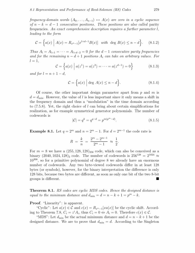
8.1 Representation and Performance of Reed-Solomon (RS) Codes 279
frequency-domain words (A0, . . . , An−1) ↔ A(x) are zero in a cyclic sequenceof n − k = d − 1 consecutive positions. These positions are also called parityfrequencies. An exact comprehensive description requires a further parameter l,leading to the form
C ={a(x)
∣∣∣ A(x) = Rxn−1[xl+d−1B(x)] with deg B(x) ≤ n− d
}. (8.1.2)
Thus Al = Al+1 = · · · = Al+d−2 = 0 for the d− 1 consecutive parity frequenciesand for the remaining n − d + 1 positions Ai can take on arbitrary values. Forl = 1,
C ={a(x)
∣∣∣ a(z1) = a(z2) = · · · = a(zd−1) = 0}
(8.1.3)
and for l = n+ 1− d,
C ={a(x)
∣∣∣ deg A(x) ≤ n− d}. (8.1.4)
Of course, the other important design parameter apart from p and m isd = dmin. However, the value of l is less important since it only means a shift inthe frequency domain and thus a “modulation” in the time domain accordingto (7.5.8). Yet, the right choice of l can bring about certain simplifications forrealization, as for example symmetrical generator polynomials. The number ofcodewords is
|C| = qk = qq−d = pm(pm−d). (8.1.5)
Example 8.1. Let q = 2m and n = 2m − 1. For d = 2m−1 the code rate is
R =k
n=
2m − 2m−1
2m − 1≈ 1
2.
For m = 8 we have a (255, 128, 128)256 code, which can also be conceived as abinary (2040, 1024, 128)2 code. The number of codewords is 256128 = 21024 ≈10308, so for a primitive polynomial of degree 8 we already have an enormousnumber of codewords. Any two byte-viewed codewords differ in at least 128bytes (or symbols), however, for the binary interpretation the difference is only128 bits, because two bytes are different, as soon as only one bit of the two 8-bitgroups is different. �
Theorem 8.1. RS codes are cyclic MDS codes. Hence the designed distance isequal to the minimum distance and dmin = d = n− k + 1 = pm − k.
Proof. “Linearity”: is apparent.“Cyclic”: Let a(x) ∈ C and c(x) = Rxn−1[xa(x)] be the cyclic shift. Accord-
ing to Theorem 7.8, Ci = ziAi, thus Ci = 0⇔ Ai = 0. Therefore c(x) ∈ C.“MDS”: Let dmin be the actual minimum distance and d = n− k+ 1 be the
designed distance. We are to prove that dmin = d. According to the Singleton

280 8. Reed-Solomon and Bose-Chaudhuri-Hocquenghem Codes
bound of Theorem 4.7, dmin ≤ n − k + 1 = d. Consider C as in (8.1.4) withdegA(x) ≤ n−d. Therefore A(x) �= 0 has a maximum of n−d roots, hence thereare a maximum of n− d values z−i with ai = −A(z−i) = 0. Thus wH(a(x)) ≥ dand dmin ≥ d. For any other l we also have dmin = d, since the “modulation” inthe time domain does not affect the weights. �
8.1.2 Polynomial and Matrix Description
Theorem 8.2. For the RS code as given in (8.1.3) the generator polynomialand the parity-check polynomial are
g(x) =
d−1∏i=1
(x− zi) , h(x) =
n∏i=d
(x− zi). (8.1.6)
Proof. For each codeword, a(zi) = 0 with 1 ≤ i ≤ d − 1. Thus (x − zi) is adivisor of a(x). So a(x) must be a multiple of g(x). Since g(x) has the degreed−1 = n−k, g(x) is the generator polynomial. For the parity-check polynomialh(x), g(x)h(x) = xn − 1 must be valid, which is the case according to (7.2.13).
�Systematic encoding can be performed with g(x) or h(x) according to the
methods discussed in Section 6.4.A further alternative is given directly by the spectral description, since non-
systematic encoding can be accomplished by inverse Fourier transform wherethe Ai values are presumed as information symbols in the frequency domain.For this realization, the encoder consists of an additive chain of k multipliersoperated in separate feedback loops, where the chain is to be run through ntimes as illustrated in Figure 7.1. So nk = n2R operations are required and theadder chain has to be computed sequentially. Usually, this IDFT method doesnot have any significant advantages over the four encoding methods discussedin Section 6.4. However, the IDFT could be simplified in certain cases by usingFFT (Fast Fourier Transform) methods.
The equation Ai = a(zi) =
n−1∑µ=0
aµziµ = 0 with 1 ≤ i ≤ d − 1 as in (8.1.3)
directly yields a (n− k, n) = (d− 1, n)-dimensional parity-check matrix H :
(a0, . . . , an−1) ·
1 z1 z2 . . . zn−1
1 z2 z4 . . . z2(n−1)
......
......
1 zd−1 z(d−1)2 . . . z(d−1)(n−1)
T
︸ ︷︷ ︸H T
= (0, . . . , 0). (8.1.7)

8.1 Representation and Performance of Reed-Solomon (RS) Codes 281
However, we do not necessarily need the parity-check matrix for decoding.
Example 8.2. Let p = 2, m = 3 and therefore n = 7. The arithmetic of F23 isthe same as in Example 7.4. For the designed distance d = 3, we have a (7, 5, 3)8RS code C = {(a0, . . . , a6) | A1 = A2 = 0}. According to Theorem 8.2,
g(x) = (x− z)(x− z2) = x2 + z4x+ z3,
h(x) = (x− z3)(x− z4)(x− z5)(x− z6)(x− z7)
= x5 + z4x4 + x3 + z5x2 + z5x+ z4.
For the generator matrix, according to (6.2.7),
G =
z3 z4 1z3 z4 1
z3 z4 1z3 z4 1
z3 z4 1
.
For the parity-check matrix, according to (6.3.3),
H1 =
(1 z4 1 z5 z5 z4
1 z4 1 z5 z5 z4
)or according to (8.1.7)
H2 =
(1 z1 z2 z3 z4 z5 z6
1 z2 z4 z6 z1 z3 z5
).
By using elementary row operations H1 can be transformed into H2: multiplyrow 2 in H1 by z2 and then add row 2 to row 1:
H3 =
(1 z1 z2 z3 z4 z5 z6
0 z2 z6 z2 1 1 z6
).
Multiplying row 2 with z2 and adding row 1 to row 2 finally yields H2. Thiscode corrects one error in the 8-ary symbols or in the binary 3-tuples. �
8.1.3 The Weight Distribution of MDS Codes
Theorem 8.3. The weight distribution as given in Definition 4.7 can be calcu-lated in an analytically closed way for any arbitrary (n, k, dmin)q MDS code andtherefore also for every RS code:
Ar =
(n
r
)(q − 1)
r−dmin∑j=0
(−1)j(r − 1
j
)qr−dmin−j (8.1.8)
=
(n
r
) r−dmin∑j=0
(−1)j(r
j
)(qr−dmin+1−j − 1). (8.1.9)
282 8. Reed-Solomon and Bose-Chaudhuri-Hocquenghem Codes
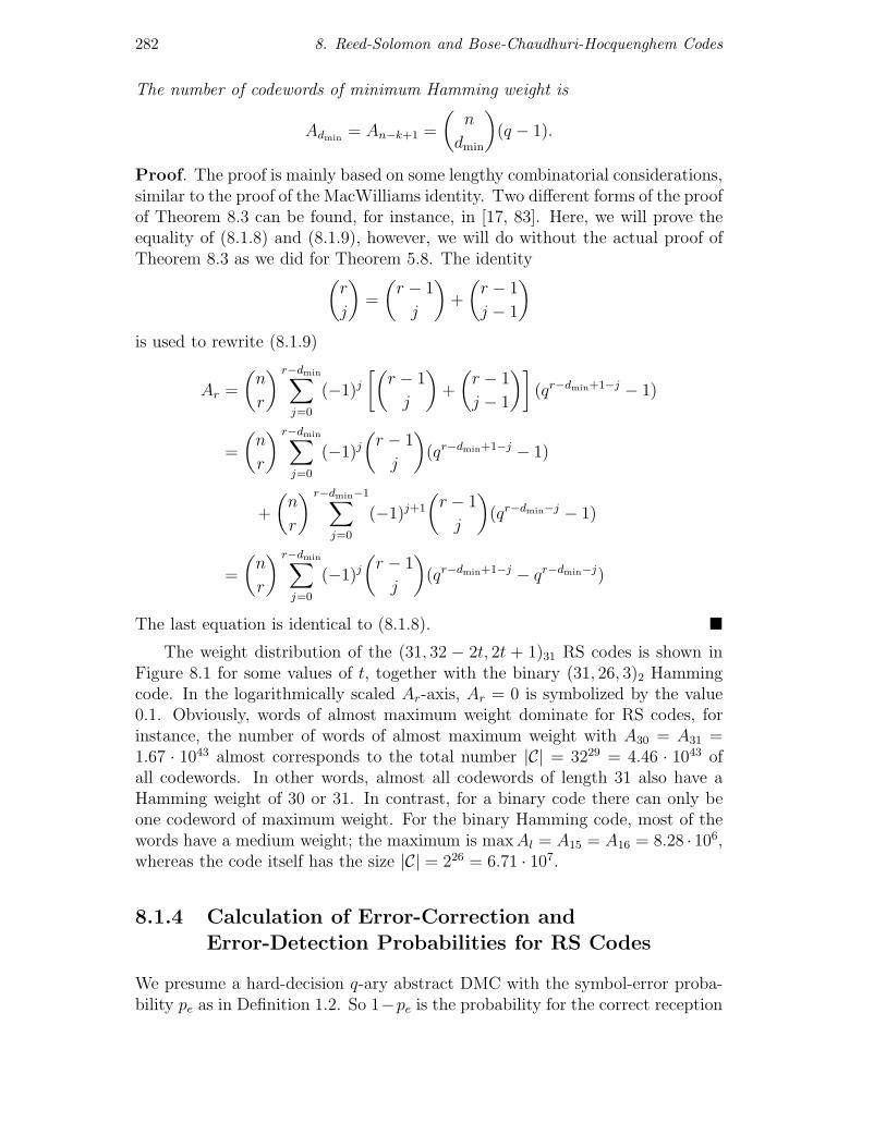
The number of codewords of minimum Hamming weight is
Admin= An−k+1 =
(n
dmin
)(q − 1).
Proof. The proof is mainly based on some lengthy combinatorial considerations,similar to the proof of the MacWilliams identity. Two different forms of the proofof Theorem 8.3 can be found, for instance, in [17, 83]. Here, we will prove theequality of (8.1.8) and (8.1.9), however, we will do without the actual proof ofTheorem 8.3 as we did for Theorem 5.8. The identity(
r
j
)=
(r − 1
j
)+
(r − 1
j − 1
)is used to rewrite (8.1.9)
Ar =
(n
r
) r−dmin∑j=0
(−1)j[(
r − 1
j
)+
(r − 1
j − 1
)](qr−dmin+1−j − 1)
=
(n
r
) r−dmin∑j=0
(−1)j(r − 1
j
)(qr−dmin+1−j − 1)
+
(n
r
) r−dmin−1∑j=0
(−1)j+1
(r − 1
j
)(qr−dmin−j − 1)
=
(n
r
) r−dmin∑j=0
(−1)j(r − 1
j
)(qr−dmin+1−j − qr−dmin−j)
The last equation is identical to (8.1.8). �The weight distribution of the (31, 32 − 2t, 2t + 1)31 RS codes is shown in
Figure 8.1 for some values of t, together with the binary (31, 26, 3)2 Hammingcode. In the logarithmically scaled Ar-axis, Ar = 0 is symbolized by the value0.1. Obviously, words of almost maximum weight dominate for RS codes, forinstance, the number of words of almost maximum weight with A30 = A31 =1.67 · 1043 almost corresponds to the total number |C| = 3229 = 4.46 · 1043 ofall codewords. In other words, almost all codewords of length 31 also have aHamming weight of 30 or 31. In contrast, for a binary code there can only beone codeword of maximum weight. For the binary Hamming code, most of thewords have a medium weight; the maximum is maxAl = A15 = A16 = 8.28 · 106,whereas the code itself has the size |C| = 226 = 6.71 · 107.
8.1.4 Calculation of Error-Correction and
Error-Detection Probabilities for RS Codes
We presume a hard-decision q-ary abstract DMC with the symbol-error proba-bility pe as in Definition 1.2. So 1−pe is the probability for the correct reception

8.1 Representation and Performance of Reed-Solomon (RS) Codes 283
0 5 10 15 20 25 30
100
105
1010
1015
1020
1025
1030
1035
1040
r
Ar
RS(31,29,3)32
RS(31,27,5)32
RS(31,23,9)32
RS(31,15,17)32
Hamming(31,26,3)2
Figure 8.1. Weight distributions of RS and Hamming codes
of a symbol, pe is the probability for an arbitrary error and pe/(q − 1) is theprobability for a specific error. The transmission over the DMC is modeled asy = a + a with the transmitted codeword a ∈ C and the error pattern e, asknown from Chapters 4 and 6.
For a bounded-minimum-distance (BMD) decoder we distinguish betweenthe following post-decoding error probabilities, which all refer to codewords, notto symbols. This is also illustrated in Figure 8.2.
(1) The probability for correct decoding is the probability that the received wordy is contained in the decoding sphere of radius t = �(dmin − 1)/2� aroundthe transmitted codeword a . By using Theorem 4.15 we get
Pcd = P (y ∈ Kt(a) | a) = P (wH(e) ≤ t) =t∑
r=0
(n
r
)pre(1−pe)
n−r. (8.1.10)
(2) The word-error probability is the probability that y is not contained in thedecoding sphere of radius t around a :
Pw = 1− Pcd = P (wH(e) > t) =n∑
r=t+1
(n
r
)pre(1− pe)
n−r. (8.1.11)

284 8. Reed-Solomon and Bose-Chaudhuri-Hocquenghem Codes
a
Pcd=1-P
wPicd
Ped
Figure 8.2. Illustration of some post-decoding error probabilities
(3) The probability of incorrect decoding is the probability that y is containedin the decoding sphere of radius t around another codeword b unequal tothe transmitted codeword a :
Picd = P
e ∈
⋃b∈C\{0}
Kt(b)
. (8.1.12)
(4) The probability of error detection is the probability that y is not containedin any of the decoding spheres of radius t around the codewords:
Ped = P
(e /∈⋃b∈C
Kt(b)
). (8.1.13)
(5) The probability of undetected error was already introduced in Section 4.6 asthe probability that y is identical to another codeword, yet unequal to thetransmitted codeword:
Pue = P (e ∈ C \ {0}). (8.1.14)
This probability is only mentioned to complete the list, since it is onlyrelevant purely for error-detection decoding without error-correction.

8.1 Representation and Performance of Reed-Solomon (RS) Codes 285
Obviously,
Pcd + Picd + Ped = 1, or equivalently Ped = Pw − Picd. (8.1.15)
For the orders of the error probabilities we typically have
Pue � Picd � Pw ≈ Ped. (8.1.16)
Furthermore, there are also the post-decoding bit error probability Pb and thepost-decoding error probability Pcs of the encoded q-ary symbols, which aresmaller than Pw by a maximum factor of k · log2 q and k, respectively, thusPw/(k log 2q) ≤ Pb ≤ Pw and Pw/k ≤ Pcs ≤ Pw. In Theorem 4.15 we stated anupper bound for Pcs
Pcs ≤ Pcs,bound =
n∑r=t+1
min
{1,
r + t
k
}(n
r
)pre(1− pe)
n−r. (8.1.17)
For the derivation of the approximation of Pcs in the proof of Theorem 4.15 weused the fact that the number of symbol errors per decoded word is limited tor + t given that the received word contains r errors. This is still exactly true,since on the one hand if the received word lies between the decoding spheres,no decoding takes place and therefore no further symbol errors can occur. Onthe other hand if the received word is in a wrong decoding sphere, there is amaximum of t further symbol errors. A slightly different bound can be found in[151]. Another approach to the problem of bit-error rate calculations is presentedin [131].
In contrast to determining the word-error rate Pw, which is very simple, thecalculation of Picd, Ped and Pue requires the knowledge of the weight distribution,which, fortunately, according to Theorem 8.3, can be calculated quite easily forall RS codes. This is why we will discuss the calculation of Picd and Ped in thischapter although it is really only an MDS specificity and does not relate to thealgebraic structure of RS codes in any way. In addition, error detection, i.e.,detecting that the received word lies between the decoding spheres, can be easilyimplemented by RS decoders, as we will see later in this chapter.
Theorem 8.4. We presuppose a q-ary hard-decision DMC with the symbol-error probability pe. For an (n, k, dmin)q MDS code with the weight distribu-tion A0, . . . , An and t = �(dmin − 1)/2� the post-decoding probability of incorrectdecoding of a received word can be exactly calculated in closed form:
Picd =n∑
h=dmin
Ah
t∑s=0
h+s∑l=h−s
N(l, s, h) · p(l), (8.1.18)
where
p(l) =
(pe
q − 1
)l(1− pe)
n−l (8.1.19)

286 8. Reed-Solomon and Bose-Chaudhuri-Hocquenghem Codes
and
N(l, s, h) =
r2∑r=r1
(h
h− s+ r
)(s− r
l − h + s− 2r
)(n− h
r
)(q − 2)l−h+s−2r(q − 1)r
(8.1.20)with r1 = max{0, l − h} and r2 = �(l − h + s)/2�. The term N(l, s, h) denotesthe number of error patterns of weight l that are at Hamming distance s to aspecific codeword b of weight h. The definition of N(l, s, h) is independent ofthe choice of b. According to (1.3.10), p(l) denotes the probability of a specificerror pattern of weight l.
Proof. For a specific b ∈ C with wH(b) = h, let
N(l, s, h) =∣∣∣{e ∈ Fn
q | wH(e) = l and dH(e,a) = s}∣∣∣,
where h− s ≤ l ≤ h+ s must be valid for N(l, s, h) > 0. The probability Picd ofincorrect decoding is the probability that e is contained in a decoding sphere ofradius t around a codeword unequal to the all-zero codeword:
Picd =∑
b∈C\{0}P (e|e is decoded to b)
=∑
b∈C\{0}
t∑s=0
P (e|dH(e, b) = s)
=∑
b∈C\{0}
t∑s=0
n∑l=0
P (e|wH(e) = l and dH(e, b) = s)
=∑
b∈C\{0}
t∑s=0
n∑l=0
N(l, s, wH(a)) · p(l)
=n∑
h=dmin
Ah
t∑s=0
h+s∑l=h−s
N(l, s, h)) · p(l).
To complete the proof we are to show the expression (8.1.20) for N(l, s, h). Wemodify b of Hamming weight h in s positions into e of Hamming weight l. Thenwe count the number of possibilities which give us the value of N(l, s, h). Tomodify b into e we divide b into five sectors:
a = (�= 0 . . . �= 0 �= 0 . . . �= 0 �= 0 . . . �= 0 0 . . . . . . 0 0 . . . . . . 0 )
different identical different different identical
e = ( 0 . . . . . . 0︸ ︷︷ ︸v
�= 0 . . . �= 0︸ ︷︷ ︸w
�= 0 . . . �= 0︸ ︷︷ ︸j
�= 0 . . . �= 0︸ ︷︷ ︸r
0 . . . . . . 0︸ ︷︷ ︸g
)

8.1 Representation and Performance of Reed-Solomon (RS) Codes 287
using g = n− v − w − j − r as an abbreviation. The following must be valid:
h = wH(a) = v + w + j
l = wH(e) = w + j + r
s = dH(a ,a) = v + j + r.
(8.1.21)
Let v, w, j, r be arbitrary. For the first h positions, i.e., for the first three sectors,
there are
(h
w
)possibilities to choose the w identical positions. For the j mod-
ifications in the remaining h − w = v + j positions there are
(h− w
j
)(q − 2)j
ways to modify the non-zero symbols into other non-zero symbols. For the last
n− h = r+ g positions, i.e., for the last two sectors, there are
(n− h
r
)(q − 1)r
ways of choosing the r non-zero symbols. All of this leads us to
N(l, s, h|v, w, j, r) =
(h
w
)·(h− w
j
)(q − 2)j ·
(n− h
r
)(q − 1)r.
The equations (8.1.21) imply that
h− s + r = w, l − h+ s− 2r = j
and therefore
N(l, s, h|r) =(
h
h− s+ r
)(s− r
l − h+ s− 2r
)(n− h
r
)(q − 2)l−h+s−2r(q − 1)r
and finally
N(l, s, h) =
r2∑r=r1
N(l, s, h|r).
Further considerations lead to r1 = max{0, l − h} and r2 = �(l − h + s)/2�, sothat the bottom numbers of the binomial coefficients are always smaller than orequal to the upper numbers and both numbers are always non-negative. �
The proof above follows the methods in [95, 131]. Slightly different butequivalent analytical expressions of Picd are derived in [17, 144].
Theorem 8.5. For the probability of incorrect decoding for a q-ary hard-decision DMC with the symbol-error probability pe the following approximationscan be made. For small pe,
Pw
Picd≈ t! · (q − 1)t
(n− 2t)(n− 2t+ 1) · · · (n− t+ 1)≈ t! ·
q − 1
n− 3
2t
t
≥ t!. (8.1.22)

288 8. Reed-Solomon and Bose-Chaudhuri-Hocquenghem Codes
For small pe and the primitive block length n = q − 1 we even have
Pw
Picd≈ t!. (8.1.23)
For large pe,
Picd ≈ q−(n−k) ·t∑
r=0
(n
r
)(q − 1)r. (8.1.24)
Proof. For small pe,
Pw =
n∑r=t+1
(n
r
)pre(1− pe)
n−r ≈(
n
t+ 1
)pt+1e .
In the expression for Picd according to (8.1.18), the summands are only dom-inant at the minimum value of l, because p(l) decreases rapidly for increasingl. According to (8.1.18), minimum l implies minimum h and maximum s, thush = 2t+ 1, s = t, l = t+ 1 as well as r1 = r2 = 0. Therefore
Picd = A2t+1
(2t+ 1
t+ 1
)(t
0
)(n− 2t− 1
0
)(q − 2)0(q − 1)0p(t+ 1)
≈ (q − 1)
(n
2t+ 1
)(2t+ 1
t+ 1
)(pe
q − 1
)t+1
,
where A2t+1 was determined according to Theorem 8.3 and the approximation1− pe ≈ 1 was used for p(l). The given form of the quotient Pw/Picd is achievedby simple remodeling and the product in the denominator, which consists of tfactors, is replaced by the power of t of the middle factor. The inequality on theright hand side of (8.1.22) follows directly from q − 1 ≥ n ≥ n− 3t/2.
For large pe the worst case is pe = (q−1)/q, since for pe/(q−1) = 1−pe = 1/q,p(l) = 1/qn which is independent of l. Thus every specific error pattern occurswith the same probability, so the channel is completely random, which allowsthe following approximation:
Picd = P (y is contained in the wrong decoding sphere)
= P (y is contained in an arbitrary decoding sphere)
− P (y is contained in the correct decoding sphere)
≈ cardinality of all decoding spheres of all codewords
number of possible words
− P (y is contained in the correct decoding sphere)
=
qk ·t∑
r=0
(n
r
)(q − 1)r
qn−
t∑r=0
(n
r
)pre(1− pe)
n−r︸ ︷︷ ︸= (q − 1)r/qn
=
(qk
qn− 1
qn
) t∑r=0
(n
r
)(q − 1)r.

8.1 Representation and Performance of Reed-Solomon (RS) Codes 289
The approximation qk − 1 ≈ qk finally leads us to the result of (8.1.22). �Both approximations of Theorem 8.5 are very precise, which we can easily
verify by the performance curves in the next subsection.
8.1.5 Performance Results for RS Codes overRandom-Error Channels
In this subsection we will only take a look at RS codes over the binary modulatedAWGN channel with hard decisions, so we assume statistically independent ran-dom single errors and the results are displayed over Eb/N0. One of the greatadvantages of RS codes is their capability of correcting burst errors, however,we will consider the corresponding performance results not in this chapter butlater on in Section 12.?.
The following figures show the performance of RS codes over q = 2m for var-ious parameter constellations, where the post-decoding error rates are displayedover Eb/N0 and pe in the upper and lower subfigures, respectively. Generally,the word-error rate Pw is always given as in (8.1.11) and the probability of in-correct decisions Picd as in (8.1.18), usually over Eb/N0 in the upper subfiguresas well as over the q-ary symbol error rate prior to the decoder pe in the bottomsubfigures. For the binary AWGN channel, i.e., for BPSK modulation, pe isdetermined by Eb/N0 as
pe = 1−(1−Q
(√2REb
N0
))m
, (8.1.25)
using (1.3.16), with m = log2 q and M = 1, as well as (1.3.23).The following upper subfigures over Eb/N0 contain not only the graphs for
the word-error rate Pw and Picd but also the bit-error rate pb,unc = Q(√
2Eb/N0)for uncoded binary signaling. Concerning the bottom subfigures over pe, theuncoded bit-error rate pb,unc could only be shown over the q-ary symbol-errorrate pe if all RS codes were considered over the same q = 2m, because of pb,unc =1−(1−pe)
1/m, of course. In actual fact, pb,unc over pe is only given in the bottompart of Figure 8.6.
The first three figures show RS codes with primitive block lengths n = q−1over q = 32, q = 64 and q = 256 for t = 1, 2, 4, 8 and partly also for t = 16 andt = 32, with k = n − 2t accordingly. Note that for n = 255 the block lengthfor binary interpretation already amounts to 2040 bits. Independent of q or n,increasing t obviously yields improvements of some dB with regards to Eb/N0.
Also, Picd rapidly decreases with increasing t, so the probability of unde-tected errors becomes quite small. For n = 255 and t = 8, Picd ≤ 2.1 · 10−5
according to (8.1.23), which can be clearly seen in Figure 8.5. FurthermorePicd ≤ 2.6 ·10−14 at t = 16 as well as Picd ≤ 3.8 ·10−37 at t = 32. For the relationPw/Picd, the approximation (8.1.22) at n = 255 gives us the values 1, 2, 26, 59291for t = 1, 2, 4, 8 which can also be seen in Figure 8.5.
290 8. Reed-Solomon and Bose-Chaudhuri-Hocquenghem Codes
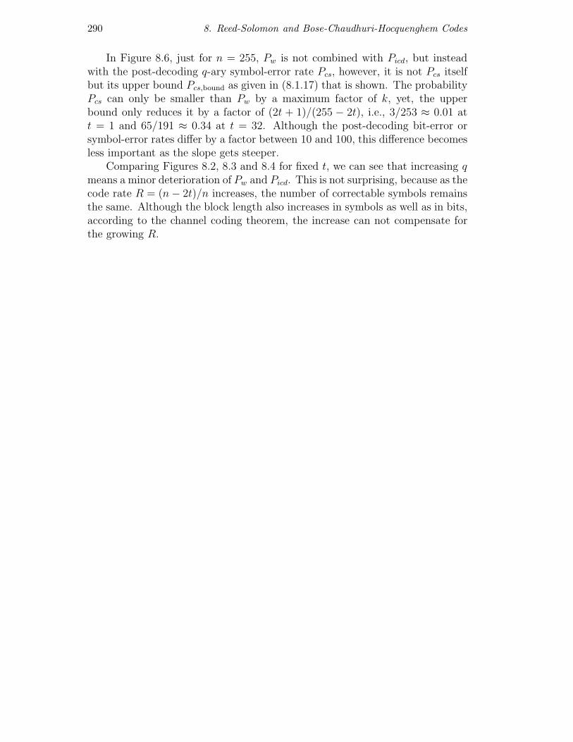
In Figure 8.6, just for n = 255, Pw is not combined with Picd, but insteadwith the post-decoding q-ary symbol-error rate Pcs, however, it is not Pcs itselfbut its upper bound Pcs,bound as given in (8.1.17) that is shown. The probabilityPcs can only be smaller than Pw by a maximum factor of k, yet, the upperbound only reduces it by a factor of (2t + 1)/(255 − 2t), i.e., 3/253 ≈ 0.01 att = 1 and 65/191 ≈ 0.34 at t = 32. Although the post-decoding bit-error orsymbol-error rates differ by a factor between 10 and 100, this difference becomesless important as the slope gets steeper.
Comparing Figures 8.2, 8.3 and 8.4 for fixed t, we can see that increasing qmeans a minor deterioration of Pw and Picd. This is not surprising, because as thecode rate R = (n− 2t)/n increases, the number of correctable symbols remainsthe same. Although the block length also increases in symbols as well as in bits,according to the channel coding theorem, the increase can not compensate forthe growing R.

8.1 Representation and Performance of Reed-Solomon (RS) Codes 291
3 4 5 6 7 8 9 10 11 12 13
10−10
10−8
10−6
10−4
10−2
100
Eb/N
0 [dB]
Pos
t−de
codi
ng e
rror
rat
es
Pw
Picd
uncoded BER
t=1
t=2 t=4
t=2
t=4
t=8
t=8
10−5
10−4
10−3
10−2
10−1
100
10−12
10−10
10−8
10−6
10−4
10−2
100
Symbol−error rate before decoder
Pos
t−de
codi
ng e
rror
rat
es
Pw
Picd
t=1
t=2
t=4
t=8
Figure 8.3. Pw and Picd of (31, 31 − 2t, 2t+ 1)32-RS codes for several t

292 8. Reed-Solomon and Bose-Chaudhuri-Hocquenghem Codes
3 4 5 6 7 8 9 10 11 12 1310
−12
10−10
10−8
10−6
10−4
10−2
100
Eb/N
0 [dB]
Pos
t−de
codi
ng e
rror
rat
es
Pw
Picd
uncoded BER
t=1 t=2 t=4 t=8 t=16
t=8
t=4 t=2
10−5
10−4
10−3
10−2
10−1
100
10−12
10−10
10−8
10−6
10−4
10−2
100
Symbol−error rate before decoder
Pos
t−de
codi
ng e
rror
rat
es
Pw
Picd
t=1
t=16
t=2
t=4
t=8
Figure 8.4. Pw and Picd of (63, 63 − 2t, 2t+ 1)64-RS codes for several t

8.1 Representation and Performance of Reed-Solomon (RS) Codes 293
3 4 5 6 7 8 9 10 11 12 1310
−12
10−10
10−8
10−6
10−4
10−2
100
Eb/N
0 [dB]
Pos
t−de
codi
ng e
rror
rat
es
Pw
Picd
t=16
uncoded BER
t=2 t=4
t=1 t=2 t=4 t=8
t=32 t=8
10−5
10−4
10−3
10−2
10−1
100
10−12
10−10
10−8
10−6
10−4
10−2
100
Symbol−error rate before decoder
Pos
t−de
codi
ng e
rror
rat
es
Pw
Picd
t=1
t=32
t=2
t=4
t=16
t=8
Figure 8.5. Pw and Picd of (255, 255 − 2t, 2t+ 1)256-RS codes for several t

294 8. Reed-Solomon and Bose-Chaudhuri-Hocquenghem Codes
3 4 5 6 7 8 9 10 11 12 1310
−12
10−10
10−8
10−6
10−4
10−2
100
Eb/N
0 [dB]
Pos
t−de
codi
ng e
rror
rat
es
Pw
Pcs,bound
t=2
uncoded BER
t=1 t=4
t=16 t=8t=32
10−5
10−4
10−3
10−2
10−1
100
10−12
10−10
10−8
10−6
10−4
10−2
100
Symbol−error rate before decoder
Pos
t−de
codi
ng e
rror
rat
es
Pw
Pcs,bound
t=4
uncoded BER
t=1
t=2
t=8 t=16t=32
Figure 8.6. Pw and Pb of (255, 255 − 2t, 2t+ 1)256-RS codes for several t

8.1 Representation and Performance of Reed-Solomon (RS) Codes 295
3 4 5 6 7 8 9 10 11 12 1310
−12
10−10
10−8
10−6
10−4
10−2
100
Eb/N
0 [dB]
Pos
t−de
codi
ng e
rror
rat
es
Pw
Picd
q=128
uncoded BER q=64
q=128 q=64
q=256
q=256
Figure 8.7. Pw and Picd of (63, 47, 17)q -RS codes for several q
In Figure 8.7 we consider shortened RS codes with n = 63 < q = 64, 128, 256.As we will see later in Theorem 8.14, shortened MDS codes are still MDS codes.Thus n−k = 2t is still valid and Pw and Picd can be calculated as usual. For fixedn = 63, k = 47 and t = 8, we increase q and therefore also the binary blocklength. The effect is a minor deterioration of Pw over Eb/N0, which is solelycaused by the increasing q-ary symbol-error rate pe, as a q-ary symbol requiresmore binary transmissions for increasing q and is therefore more vulnerable toerrors. However, over pe, Pw is fully independent of q, which is obvious lookingat (8.1.11). In contrast to Pw, Picd undergoes a significant improvement forincreasing q.
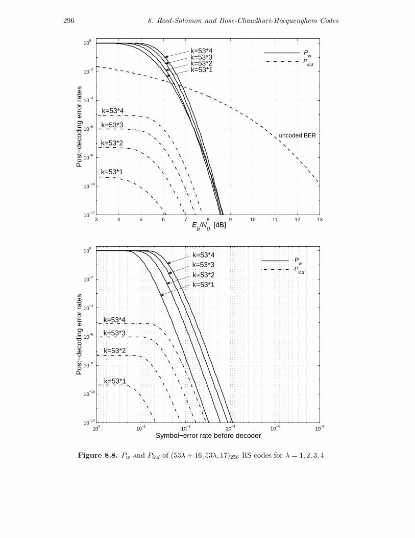
In Figure 8.8 we examine the shortening under different circumstances. Wehave q = 256 and t = 8 fixed, but the block length is n = 53λ + 2t, so a codeblock transports either 1, 2, 3 or 4 ATM cells [?]. Small λ implies a smaller blocklength and a decreasing code rate and thus worse bandwidth efficiency, however,the power efficiency, i.e., Pw over Eb/N0, remains almost the same. Over pe(bottom subfigure) instead of over Eb/N0 (upper subfigure), the dependence onthe code rate does not exist, so small λ is the most suitable, because the coderate is small without paying the penalty of worsening signal-to-noise ratio.
296 8. Reed-Solomon and Bose-Chaudhuri-Hocquenghem Codes
3 4 5 6 7 8 9 10 11 12 1310
−12
10−10
10−8
10−6
10−4
10−2
100
Eb/N
0 [dB]
Pos
t−de
codi
ng e
rror
rat
es
Pw
Picd
k=53*4
uncoded BER
k=53*4
k=53*1 k=53*2 k=53*3
k=53*3
k=53*1
k=53*2
10−5
10−4
10−3
10−2
10−1
100
10−12
10−10
10−8
10−6
10−4
10−2
100
Symbol−error rate before decoder
Pos
t−de
codi
ng e
rror
rat
es
Pw
Picd
k=53*4
k=53*1
k=53*3
k=53*2
k=53*1
k=53*2
k=53*3
k=53*4
Figure 8.8. Pw and Picd of (53λ+ 16, 53λ, 17)256-RS codes for λ = 1, 2, 3, 4

8.1 Representation and Performance of Reed-Solomon (RS) Codes 297
3 4 5 6 7 8 9 10 11 12 1310
−12
10−10
10−8
10−6
10−4
10−2
100
Eb/N
0 [dB]
Pos
t−de
codi
ng e
rror
rat
es
Pw
Picd
uncoded BER
t=2
t=32 t=64
t=4 t=8 t=16
t=2
t=4
t=8
10−5
10−4
10−3
10−2
10−1
100
10−12
10−10
10−8
10−6
10−4
10−2
100
Symbol−error rate before decoder
Pos
t−de
codi
ng e
rror
rat
es
Pw
Picd
t=4
t=32
t=8
t=16
t=2
t=64
t=8
t=2 t=4
Figure 8.9. Pw and Picd of (4t− 1, 2t− 1, 2t + 1)4t-RS codes for several t

298 8. Reed-Solomon and Bose-Chaudhuri-Hocquenghem Codes
Finally, Figure 8.9 shows a comparison of non-shortened RS codes again.We consider RS codes over q = 8, 16, 32, 64, 128, 256 with code rate R = 1/2 inthe form (4t− 1, 2t− 1, 2t+ 1)4t. Obviously, we gain a lot thanks to increasingblock length and thus to increasing complexity. However, at t = 64 the perfor-mance curve is already very steep with less than 1 dB between almost error freetransmission and total failure. We will discuss the practical side of such curvesin Section 10.?.
8.2 Representation and Performance of
Bose-Chaudhuri-Hocquenghem (BCH)
Codes
We will first introduce BCH codes as a subset of RS codes. Some examplesand interesting special cases are considered in Subsection 8.2.2. Tables andperformance curves of very high practical relevance are presented in Subsection8.2.3. Finally, the asymptotic properties of BCH codes and further features areconsidered in Subsection 8.2.4.
8.2.1 Definition of BCH Codes as Subsets of RS Codes
BCH codes emerge from RS codes by adopting the Fourier transform in Fpm andthe block length n = pm − 1, but the code symbols are taken from the primefield Fp instead of Fpm. For the typical case of p = 2 the code symbols are bitsand not groups of bits, so BCH codes are normal binary codes for p = 2.
Definition 8.2 (BCH codes). For arbitrary prime p and integer m and anarbitrary designed distance d, a Bose-Chaudhuri-Hocquenghem code is definedas an (n, k, dmin)p code with the primitive block length n = pm − 1 = q − 1 andthe relations
dmin ≥ d , k ≤ n+ 1− dmin ≤ n+ 1− d. (8.2.1)
Thus n − k ≥ 2t for d = 2t + 1. The code consists of all time-domainwords (a0, . . . , an−1) ↔ a(x) with coefficients in Fp, such that the correspondingfrequency-domain words (A0, . . . , An−1)↔ A(x) are zero in a cyclic sequence ofat least d− 1 consecutive positions. Usually the parity frequencies are presumedat 1, . . . , d− 1 and the resulting code
C ={a(x) ∈ Fp[x]
∣∣∣ a(z1) = · · · = a(zd−1) = 0}
(8.2.2)
is then called a narrow-sense BCH code. As for the RS codes, the exact de-scription of general BCH codes requires a further parameter l, where the parityfrequencies are defined by Al = Al+1 = · · · = Al+d−2 = 0 for the d−1 consecutivepositions.

8.2 Representation and Performance of BCH Codes 299
From the given designed distance d we do not directly obtain the informationblock length k or the code rate R nor the actual minimum distance dmin, buthave to calculate these parameters first. The parameter l for determining theparity frequencies is of greater importance for BCH codes than for RS codes,since for BCH codes l might even influence dmin. However, typically the narrow-sense BCH codes as in (8.2.2) are used, because then the number of parity bitsis usually at its minimum.
In contrast to (8.1.3) with a(x) ∈ Fpm [x] for RS codes, a(x) ∈ Fp[x] is requiredin (8.2.2) for BCH codes, both with degrees ≤ n−1. So a BCH code is a subsetof an RS code, thus dmin,BCH ≥ dmin,RS = d and the Singleton bound implies(8.2.1). The relation dmin ≥ d is also called BCH bound . Usually, dmin is notcalculated exactly, since the gap between dmin and d might remain unknown formost applications. In some cases even dmin = d is valid (see [83, 105]). The exactcalculation of the information block length k (or the dimension of the code) isperformed by the generator polynomial as follows.
Theorem 8.6. Let z be a primitive element of the Galois field Fpm. For thedesigned distance d, an (n, k, dmin)p BCH code with dmin ≥ d is created by thegenerator polynomial
g(x) = LCM(f[z1](x), . . . , f[zd−1](x)
)(8.2.3)
=∏b∈M
(x− b) with M =
d−1⋃i=1
[zi],
where [zi] = {zip0, zip1 , zip2 , . . .} denotes the set of conjugates as introduced inDefinition 7.3, i.e., all conjugates of zi with respect to Fp. The correspondingminimal polynomial is
f[zi](x) =∏b∈[zi]
(x− b) =
|[zi]|−1∏r=0
(x− zipr
). (8.2.4)
So, the generator polynomial g(x) is the least common multiple (LCM) of theminimal polynomials of z1, . . . , zd−1. Thus, for the information block length
k = n− deg g(x) = n−∣∣∣∣∣d−1⋃i=1
[zi]
∣∣∣∣∣ (8.2.5)
≥ n−d−1∑i=1
|[zi]|.
Proof. The coefficients of the minimal polynomials, and thus also of the gen-erator polynomial, are taken from the prime field Fp. So with the informationpolynomial, the codeword polynomial also has its coefficients in Fp. For each
300 8. Reed-Solomon and Bose-Chaudhuri-Hocquenghem Codes
combination of two minimal polynomials of (8.2.3), the polynomials are eitherrelatively prime or identical. As for the RS codes, the equation a(zi) = Ai = 0implies that g(x) must consist of the linear factors (x− zi) or that g(x) must be
a multiple of
d−1∏i=1
(x− zi). According to Theorem 7.9, the requirement that the
coefficients of a(x) must be in Fp is equivalent to a(zi)p = a(zip) for 0 ≤ i ≤ n−1.Thus for 1 ≤ i ≤ d− 1,
0 = a(zi)0 = a(zi)p = a(zip)
0 = a(zip)p = a(zip2)
0 = a(zip2)p = a(zip
3) . . .
So all (x− zipr) with 1 ≤ i ≤ d− 1 and r = 0, 1, 2, . . . must be linear factors of
g(x), but only once for each factor. According to (8.2.3), g(x) is reducible intojust these factors. �
For this representation, the BCH codes are defined as subsets of RS codeswhich almost makes the BCH bound dmin ≥ d seem trivial. However, there areother concepts for introducing BCH codes. For example, if the BCH codes aredefined by the generator polynomial g(x) with coefficients in Fp and its roots arez1, . . . , zd−1, then the proof of the BCH bound is quite time-consuming [144].
To make things a little easier, we introduced BCH codes with a slight re-striction in this chapter, as we did with the algebraic foundations in Chapter7 where we only discussed the extension of a prime field Fp to a Galois fieldFpm . However, the concept of field extensions over primitive polynomials can begeneralized to the extension of Fpm to Fpmr , where r is an integer, which gives usBCH codes with the primitive block length pmr−1 and pm-ary symbols. For thebinary interpretation with p = 2, the block length is simply m(2mr − 1). TheseBCH codes• are especially suitable for channels with burst errors of length m, in other
words, the coding scheme can be adjusted to the error structure of thechannel quite precisely;
• include the RS codes as a special case for r = 1, hence, BCH codes are ageneralization of RS codes and vice versa.
However, since almost all BCH codes used in practice are binary with the blocklength 2m − 1 and r = 1, the restriction chosen in Definition 8.2 seems to bereasonable under practical aspects. Thus BCH codes are still special RS codes.
The weight distribution of most BCH codes is not known analytically. BCHcodes for correcting up to 3 errors are an exception however, since formulas tocalculate the weight distribution are well known [79, 144].

8.2 Representation and Performance of BCH Codes 301
8.2.2 Examples and Special Cases
Example 8.3. As in Example 8.2, let p = 2, m = 3 and thus n = 7. For thedesigned distance d = 3 we have a narrow-sense BCH code with the generatorpolynomial
g(x) = LCM(f[z1](x), f[z2](x)
)= f[z](x) = x3 + x+ 1,
since, according to Example 7.4, [z1] = {z1, z2, z4} = [z2] with f[z](x) = x3 +x + 1. The BCH code turns out to be a cyclic (7, 4, 3)2 Hamming code, whencompared to 6.3. For better understanding, we will now take a closer lookat the representation in the frequency domain. According to Definition 8.2,A1 = A2 = 0 and according to Theorem 7.9, A2
i = A2i mod 7, as already used forthe proof of Theorem 8.6. Thus,
A0 = A2·0 = A20 implies that A0 ∈ {0, 1}
A3 = A2·5 = A25
A6 = A2·3 = A23 A3 determines A6
A5 = A2·6 = A26 = A4
3 A3 determines A5
A1 = A2·4 = A24 A1 = 0 per definition
A2 = A2·1 = A21 A2 = 0 per definition
A4 = A2·2 = A22 implies that A4 = 0.
Therefore for the codewords in the frequency domain
C ◦—• {(A0, 0, 0, A3, 0, A43, A
23) | A0 ∈ F2, A3 ∈ F8}.
With A0 ∈ F2 (1 bit) and A3 ∈ F23 (3 bits), 4 bits can be given arbitrarily in thefrequency domain, which, of course, correspond to the k = 4 information bitsin the time domain. Table 8.1 lists the corresponding frequency words to the16 codewords of the cyclic Hamming (or BCH) code of Example 6.1. ObviouslyA0 ∈ F2, A3 ∈ F8, A6 = A2
3 and A5 = A26 are satisfied and each of the 16 frequency
words of the form (A0, 0, 0, A3, 0, A43, A
23) is presented in the table. For the cyclic
shift from row to row, Ai is always multiplied by zi. �
Example 8.4. Comparison of the error-correction ability of RS and BCH codes.There exists a (15, 11, 5)16 RS code that can correct 2 symbol errors. In thebinary interpretation we have a (60, 44, 5)2 code, where
e = 0000 1111 1111 0000 0000 . . . is correctable
e = 0000 0001 1111 1000 0000 . . . is not correctable
e = 0000 0001 0010 1000 0000 . . . is not correctable.
Each burst error up to length 5 can be corrected, for burst errors of length 6, 7and 8, 75%, 50% and 25% can be corrected, respectively. However, 3 random

302 8. Reed-Solomon and Bose-Chaudhuri-Hocquenghem Codes
single errors can not be corrected. So the minimum distance for the binaryinterpretation is still 5, however, in special cases some slightly larger values arepossible but not guaranteed.
According to Table 8.2, there exists a (63, 45, 7)2 BCH code with comparablecode rate, which can always correct 3 random single errors. For a channel withburst errors, the RS code is better than the BCH code. However, for a channelwith statistically independent random single errors the BCH code is better thanthe RS code. �
Special case. In Theorem 6.10 we defined CRC codes by the generator poly-nomial g(x) = (1 + x)p(x) with a primitive polynomial p(x). For p(x) = f[z](x)CRC codes turn out to be special BCH codes with the form
g(x) = LCM(f[z0](x), f[z1](x)
)= (x+ 1)p(x) (8.2.6)
for the designed distance d = 3. Thus dmin ≥ 3. In the proof of Theorem 6.10dmin was determined to be even, so now we can exactly prove that dmin ≥ 4 ordmin = 4. �
For binary BCH codes with d = 2t + 1 the advantages of the form givenin (8.2.2) become immediately clear: a(zt) = 0 implies that a(zd−1) = a(z2t) =a(zt)2 = 0. For narrow-sense BCH codes with l = 1 (beginning at z1) at leastthe set z1, . . . , z2t of roots is required. In contrast to shifted parity frequencieswith l = 0 (beginning at z0) at least the set z0, . . . , z2t of roots is required,
Table 8.1. Time-domain codewords and corresponding frequency-domain words forthe (7, 4, 3)2 Hamming (or BCH) code
a(x) A(x)0 0 0 0 0 0 0 0 0 0 0 0 0 01 1 1 1 1 1 1 1 0 0 0 0 0 01 1 0 1 0 0 0 1 0 0 z4 0 z2 z0 1 1 0 1 0 0 1 0 0 1 0 1 10 0 1 1 0 1 0 1 0 0 z3 0 z5 z6
0 0 0 1 1 0 1 1 0 0 z6 0 z3 z5
1 0 0 0 1 1 0 1 0 0 z2 0 z z4
0 1 0 0 0 1 1 1 0 0 z5 0 z6 z3
1 0 1 0 0 0 1 1 0 0 z 0 z4 z2
1 1 1 0 0 1 0 0 0 0 z6 0 z3 z5
0 1 1 1 0 0 1 0 0 0 z2 0 z z4
1 0 1 1 1 0 0 0 0 0 z5 0 z6 z3
0 1 0 1 1 1 0 0 0 0 z 0 z4 z2
0 0 1 0 1 1 1 0 0 0 z4 0 z2 z1 0 0 1 0 1 1 0 0 0 1 0 1 11 1 0 0 1 0 1 0 0 0 z3 0 z5 z6

8.2 Representation and Performance of BCH Codes 303
thus a further factor x−1 occurs in the generator polynomial which reduces thedimension k unnecessarily. This only really makes sense for CRC codes, as seenpreviously.
Special case: We consider binary BCH codes for the correction of one error,so t = 1, d = 3 and n = 2m − 1. Again, let p(x) be a primitive polynomial andz be a primitive element of Fpm. Because of z2
m= zn+1 = z, we have
[z] = {z, z2, z4, z8, . . . , z2m−1} , |[z]| = m
for the set of conjugates of z. Thus [z] = [z2], so p(x) = f[z](x) = f[z2](x) for theminimal polynomials. According to Theorem 8.6, the generator polynomial is
g(x) = LCM(f[z1](x), f[z2](x)
)= f[z](x) =
m−1∏i=0
(x− z2i
). (8.2.7)
The last equation follows from (7.3.6). Now, according to (8.2.5),
k = n− deg g(x) = (2m − 1)−m,
so the binary BCH codes for correcting one error are (2m − 1, 2m −m − 1, 3)2codes, which correspond to the cyclic binary Hamming codes of order m, as thecomparison to Theorem 5.10 reveals. The binary Hamming codes can also bedescribed by
C = {a ∈ Fnp | a(z) = 0}
because for coefficients in the prime field, a(z) = 0 directly implies that a(z2) =a(z)2 = 0. �
Parity-check matrices of BCH codes have a special feature which we willexamine for the case of p = 2 and d = 2t + 1. As for RS codes in (8.1.7), eachrow of H also has the form z0, zi, zi·2, . . . , zi·(n−1) for BCH codes, where i takeson each of the n− k exponents in [z1]∪ . . .∪ [z2t]. However, with the conditiona(x) ∈ F2[x], i only has to take on the values 1, 2, 3, . . . , 2t. Because of
z2 ∈ [z1], z4 ∈ [z1], z6 ∈ [z3], z8 ∈ [z1], z10 ∈ [z5], . . .
i can be further restricted to the t values 1, 3, 5, . . . , 2t − 1, i.e., the dimensionof the parity-check matrix is reduced from (n − k, n) to (t, n) or to (mt, n) forthe binary interpretation. However, since mt can be greater than n − k (seeTheorem 8.8), the reduced binary parity-check matrix may still have linearlydependent rows, as we will demonstrate in Example 8.5.
Example 8.5. The next subsection contains the Tables 8.1 and 8.2, which havebeen mentioned so often and list the existing BCH codes and their error cor-rection ability. The following examples show how these tables were created.Therefore we will now consider various BCH codes with n = 15, where the

304 8. Reed-Solomon and Bose-Chaudhuri-Hocquenghem Codes
arithmetic of F24 is based on the primitive element z with z4 + z + 1 = 0 as inExample 7.5.
(1) The designed distance d = 3 implies the generator polynomial
g(x) = LCM(f[z1](x), f[z2](x)
)= f[z](x) = x4 + x+ 1,
because [z1] = {z1, z2, z4, z8} = [z2]. The result is the (15, 11, 3)2 Hammingcode. Since d = 3 ≤ dmin ≤ wH(g(x)) = 3, d = dmin as well as n− k = mt.
(2) The designed distance d = 5 implies the generator polynomial
g(x) =∏b∈M
(x− b) with M = [z1] ∪ [z2] ∪ [z3] ∪ [z4].
We have [z1] = {z1, z2, z4, z8} = [z2] = [z4] and [z3] = {z3, z6, z12, z24 = z9},thus M = [z] ∪ [z3]. Therefore the generator polynomial is
g(x) = f[z](x) · f[z3](x)= (x− z1)(x− z2)(x− z4)(x− z8)︸ ︷︷ ︸
x4 + x+ 1
· (x− z3)(x− z6)(x− z9)(x− z12)︸ ︷︷ ︸x4 + x3 + x2 + x+ 1
= x8 + x7 + x6 + x4 + 1,
which gives us a (15, 7, 5)2 code. Since d = 5 ≤ dmin ≤ wH(g(x)) = 5, d = dmin
as well as n− k = mt again. The parity-check matrix is reduced from
H =
1 z1 z1·2 . . . z1·14
1 z2 z2·2 . . . z2·14
1 z3 z3·2 . . . z3·14
1 z4 z4·2 . . . z4·14
to
H =
(1 z1 z1·2 . . . z1·14
1 z3 z3·2 . . . z3·14
).
For the binary interpretation this is a (2 ·4, 15) = (n−k, n)-dimensional matrix.(3) The designed distance d = 7 implies the generator polynomial
g(x) =∏b∈M
(x− b) with M = [z1] ∪ [z2] ∪ [z3] ∪ [z4] ∪ [z5] ∪ [z6].
Since [z1] = [z2] = [z4] and [z3] = [z6], M = [z1] ∪ [z3] ∪ [z5] thus
g(x) = f[z](x) · f[z3](x)︸ ︷︷ ︸x8 + x7 + x6 + x4 + 1
· f[z5](x)︸ ︷︷ ︸x2 + x+ 1
= x10 + x8 + x5 + x4 + x2 + x+ 1,

8.2 Representation and Performance of BCH Codes 305
which gives us a (15, 5, 7)2 code with d = dmin as well as n−k = 10 < 4 ·3 = mt.The reduced parity-check matrix is
H =
1 z1 z1·2 . . . z1·14
1 z3 z3·2 . . . z3·14
1 z5 z5·2 . . . z5·14
,
which is a (12, 15)-dimensional matrix for binary interpretation. A (15, 5)2 codehas a (10, 15)-dimensional binary parity-check matrix, so that two linearly de-pendent rows of the 12 rows of the binary H can be eliminated to get thestandard form.
(4) The designed distance d = 9 implies the generator polynomial
g(x) =∏b∈M
(x− b) with M =8⋃i=1
[zi].
Since [z1] = [z2] = [z4] = [z8] and [z3] = [z6], M = [z1] ∪ [z3] ∪ [z5] ∪ [z7] andtherefore
g(x) = f[z](x) · f[z3](x) · f[z5](x)︸ ︷︷ ︸x10 + x8 + x5 + x4 + x2 + x+ 1
· f[z7](x)︸ ︷︷ ︸x4 + x3 + 1
=x15 − 1
x− 1
= x14 + x13 + x12 + x11 + x10 + x9 + x8 + x7 + x6 + x5
+ x4 + x3 + x2 + x+ 1.
which gives us a (15, 1, 15)2-repetition code, i.e., 7 instead of simply 4 errors canbe corrected. So there are binary BCH codes of length 15 simply for correcting1, 2, 3 or 7 errors.
These 3 codes (except for the repetition code) can also be taken from thefollowing Tables 8.1 and 8.2. If the parity frequencies are moved, codes withdifferent generator polynomial may emerge. �
8.2.3 Tables and Performance Results on BCH Codes
Table 8.2 lists the binary narrow-sense BCH codes for the correction of t errorswith all primitive block lengths from n = 7 to n = 1023 [95, 105, 144, 151]. Ofcourse, 2t+ 1 ≤ d ≤ dmin ≤ n− k + 1.
Table 8.3 shows the generator polynomials in octal coding for some of theBCH codes listed in Table 8.2. For the (15, 7)2 BCH code with t = 2, forexample, we have g(x) = 721octal = 111 010 001dual = x8 + x7 + x6 + x4 + 1.

306 8. Reed-Solomon and Bose-Chaudhuri-Hocquenghem Codes
Table 8.2. t-error-correcting (n, k)2 BCH codes (from [105])
n k t n k t n k t n k t n k t7 4 1 255 199 7 511 322 22 1023 913 11 1023 443 73
191 8 313 23 903 12 433 7415 11 1 187 9 304 25 893 13 423 75
7 2 179 10 295 26 883 14 413 775 3 171 11 286 27 873 15 403 78
163 12 277 28 863 16 393 7931 26 1 155 13 268 29 858 17 383 82
21 2 147 14 259 30 848 18 378 8316 3 139 15 250 31 838 19 368 8511 5 131 18 241 36 828 20 358 866 7 123 19 238 37 818 21 348 87
115 21 229 38 808 22 338 8963 57 1 107 22 220 39 798 23 328 90
51 2 99 23 211 41 788 24 318 9145 3 91 25 202 42 778 25 308 9339 4 87 26 193 43 768 26 298 9436 5 79 27 184 45 758 27 288 9530 6 71 29 175 46 748 28 278 10224 7 63 30 166 47 738 29 268 10318 10 55 31 157 51 728 30 258 10616 11 47 42 148 53 718 31 248 10710 13 45 43 139 54 708 34 238 1097 15 37 45 130 55 698 35 228 110
29 47 121 58 688 36 218 111127 120 1 21 55 112 59 678 37 208 115
113 2 13 59 103 61 668 38 203 117106 3 9 63 94 62 658 39 193 11899 4 85 63 648 41 183 11992 5 511 502 1 76 85 638 42 173 12285 6 493 2 67 87 628 43 163 12378 7 484 3 58 91 618 44 153 12571 9 475 4 49 93 608 45 143 12664 10 466 5 40 95 598 46 133 12757 11 457 6 31 109 588 47 123 17050 13 448 7 28 111 578 49 121 17143 14 439 8 19 119 573 50 111 17336 15 430 9 10 127 563 51 101 17529 21 421 10 553 52 91 18122 23 412 11 1023 1013 1 543 53 86 18315 27 403 12 1003 2 533 54 76 1878 31 394 13 993 3 523 55 66 189
385 14 983 4 513 57 56 191255 247 1 376 15 973 5 503 58 46 219
239 2 367 16 963 6 493 59 36 223231 3 358 18 953 7 483 60 26 239223 4 349 19 943 8 473 61 16 247215 5 340 20 933 9 463 62 11 255207 6 331 21 923 10 453 63

8.2 Representation and Performance of BCH Codes 307
Table 8.3. Generator polynomials for t-error-correcting (n, k)2 BCH codes (from[221])
n k t g(x) octal7 4 1 1315 11 1 23
7 2 7215 3 2467
31 26 1 4521 2 355116 3 10765711 5 54233256 7 313365047
63 57 1 10351 2 1247145 3 170131739 4 16662356736 5 103350042330 6 15746416554724 7 1732326040444118 10 1363026512351725
127 120 1 211113 2 41567106 3 1155474399 4 344702327192 5 62473002232785 6 13070447632227378 7 2623000216613011571 9 625501071325312775364 10 120653402557077310004557 11 33526525250570505351772150 13 54446512523314012421501421
255 247 1 435239 2 267543231 3 156720665223 4 75626641375215 5 23157564726421207 6 16176560567636227199 7 7633031270420722341191 8 2663470176115333714567187 9 52755313540001322236351179 10 22624710717340432416300455171 11 15416214212342356077061630637163 12 7500415510075602551574724514601155 13 3757513005407665015722506464677633147 14 1642130173537165525304165305441011711139 15 461401732060175561570722730247453567445131 18 215713331471510151261250277442142024165471

308 8. Reed-Solomon and Bose-Chaudhuri-Hocquenghem Codes
For the entries of Tables 8.1 and 8.2 the designed distance d = 2t + 1 waspresumed. The actual minimum distance dmin is unknown and may even bemuch larger. However, most of the decoding methods for BCH codes can notprofit from a larger dmin, since the decoding is only based on the positions ofthe d− 1 = 2t sequential parity frequencies. Yet, in some cases we can calculatedmin exactly, as Theorem 8.7 proves.
Theorem 8.7. Suppose an (n, k)p BCH code with the primitive block lengthn = pm − 1. If the designed distance d is a divisor of n, then dmin = d.
Proof. Let n = d · β. The sum (5.1.2) of the finite geometric series can bedenoted by
xn − 1 = xdβ − 1 = (xβ − 1) ·(1 + xβ + x2β + · · ·+ x(d−1)β
)︸ ︷︷ ︸
= a(x)
.
For i = 1, . . . , d − 1, the relation 0 < iβ < n is valid and therefore ziβ �= 1.Since zi is a root of xn − 1 but not of xβ − 1, a(zi) = 0 must be satisfied. Sincea(x) ∈ Fp[x] and deg a(x) ≤ n − 1, a(x) is a codeword of Hamming weight d.Thus dmin ≤ d. Finally, the BCH bound dmin ≥ d leads to dmin = d. �
According to Table 8.2, n − k = m · t for small t. Typically, the requirednumber of parity-check bits is upper bounded by the minimum number of errorsto be corrected:
Theorem 8.8. For a binary (n, k)2 BCH code with the primitive block lengthn = 2m − 1, which can correct at least t errors,
n− k ≤ m · t. (8.2.8)
Proof. For the designed distance d = 2t + 1, n − k = deg g(x) is equal to
the cardinality of M =d−1⋃i=1
[zi] =t⋃
i=1
([z2i−1] ∪ [z2i]
). In F2m , zi and z2i are
conjugates, thus [zi] = [z2i]. So the conjugacy class [z2i] can be omitted and Mis reduced to M =
t⋃i=1
[z2i−1]. According to (6.3.5), |[z2i−1]| ≤ m and therefore
|M| ≤ t ·m. �
According to (7.3.1) with t ≈ dmin
2implies that 1−R ≤ m
2· dmin
n. So if
approximate equality was reached, then obviously dmin/n → 0 is implied forn → ∞ or m → ∞. Consequently, according to Section 3.4, BCH codes areasymptotically bad. A complete proof can be found in [83].
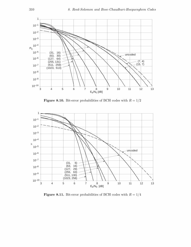
Figures 8.9, 8.10 and 8.11 show the bit-error rate over the binary modulatedAWGN channel for binary BCH codes at rates of approximately 1/2, 1/4 and

8.2 Representation and Performance of BCH Codes 309
3/4 for various block lengths between 15 and 1023. BMD decoding with harddecisions is assumed, such that the curves can be calculated according to (4.7.4).Obviously a larger block length implies a smaller error rate. The comparison ofFigures 8.9, 8.10 and 8.11 suggests R ≈ 1/2 as the best available code rate. Tomake this really clear, Figure 8.13 illustrates some BCH codes with various coderates and a constant block length of n = 255. According to the Shannon theory,small code rates are best (for example, according to Figure 3.6 a transition fromR = 1/2 to R = 1/10 can achieve a gain of approximately 1 dB), but obviouslythe construction method for BCH codes requires medium code rates for bestresults.
Both parts of Figure 8.14 show the same BCH codes with n = 255 as Figure8.13. However, the bottom part now restricts the bit-error rate to a maximumof 10−10 for easier comparison with Figures 8.9 to 8.11. In addition the top partof Figure 8.14 shows the word-error rates. According to Theorem 4.15 or (1.7.2),we have
Pb ≈ dmin
k· Pw,
so the differences between Pb and Pw are the largest for small t in Figure 8.14.For Figures 8.9 to 8.11 the differences between Pb and Pw are much smallersince an increasing t means an increase of k, so this does not merit furtherexplanation. The comparison of Figures 8.11 and Figure 8.15 will also showthat these differences are negligible.
310 8. Reed-Solomon and Bose-Chaudhuri-Hocquenghem Codes
3 4 5 6 7 8 9 10 11 12 13Eb/N0 [dB]
10–10
10–9
10–8
10–7
10–6
10–5
10–4
10–3
10–2
10–1
1
uncoded
(7, 4)(15, 7)
Pb
(31, 16)(63, 30)
(127, 64)(255, 131)(511, 259)
(1023, 513)
Figure 8.10. Bit-error probabilities of BCH codes with R = 1/2
1
10–1
10–2
10–3
10–4
10–5
10–6
10–7
10–8
10–9
10–10
3 4 5 6 7 8 9 10 11 12 13Eb/N0 [dB]
b
(31, 6)(63, 16)
(127, 29)(255, 63)(511, 130)
(1023, 258)
uncoded
Figure 8.11. Bit-error probabilities of BCH codes with R = 1/4

8.2 Representation and Performance of BCH Codes 311
uncoded
3 4 5 6 7 8 9 10 11 12 13
1
10–1
10–2
10–3
10–4
10–5
10–6
10–7
10–8
10–9
10–10
Pb
Eb/N0 [dB]
(31, 21)(63, 45)
(127, 99)(255, 191)(511, 385)
(1023, 768)
Figure 8.12. Bit-error probabilities of BCH codes with R = 3/4
uncoded
Ga = 2.9 R = 0.97 t = 1Ga = 4.5 R = 0.94 t = 2Ga = 6.4 R = 0.87 t = 4Ga = 8.3 R = 0.75 t = 8Ga = 9.9 R = 0.51 t = 18Ga = 9.7 R = 0.36 t = 25Ga = 9.0 R = 0.18 t = 42Ga = 6.6 R = 0.08 t = 55
3 4 5 6 7 8 9 10 11 12 13 14 15Eb/N0 [dB]
1
10–5
10–10
10–15
10–20
Pb
Figure 8.13. Bit-error probabilities of BCH codes with n = 255

312 8. Reed-Solomon and Bose-Chaudhuri-Hocquenghem Codes
3 4 5 6 7 8 9 10 11 12 1310
−10
10−9
10−8
10−7
10−6
10−5
10−4
10−3
10−2
10−1
100
Eb/N
0 [dB]
Wor
d−er
ror
rate
Pw
t=1t=2t=4t=8t=18t=25t=42t=55
uncoded
3 4 5 6 7 8 9 10 11 12 1310
−10
10−9
10−8
10−7
10−6
10−5
10−4
10−3
10−2
10−1
100
Eb/N
0 [dB]
Bit−
erro
r ra
te P
b
t=1t=2t=4t=8t=18t=25t=42t=55
uncoded
Figure 8.14. Word-error and bit-error probabilities of BCH codes with n = 255(same codes as in Figure 8.13)

8.2 Representation and Performance of BCH Codes 313
8.2.4 Further Considerations and Asymptotic
Properties
Figure 8.15 shows a comparison between a binary BCH code and three RScodes, where R ≈ 3/4 is the code rate for all cases. Again the binary AWGNchannel with hard decisions is presupposed, so there are no burst errors, onlyrandom single errors. For the same nominal block length the RS code is betterthan the BCH code. However, when compared to the RS block length withbinary interpretation, the BCH code is better, as expected on the grounds ofthe previous considerations and in particular Example 8.4.
3 4 5 6 7 8 9 10 11 12 1310
−12
10−10
10−8
10−6
10−4
10−2
100
Eb/N
0 [dB]
W
ord−
erro
r ra
te P
w
uncoded
RS(31,23)32
≅ (155,115)2, t=4
RS(63,47)64
≅ (378,282)2, t=8
RS(255,191)256
≅ (2040,1528)2, t=32
BCH(255,191)2, t=8
Figure 8.15. Comparison of a BCH code with some RS codes (all with R ≈ 3/4)
Note that Figure 8.15 also shows the word-error rate and Figure 8.12 thebit-error rate; the small difference for the BCH code corresponds exactly to thedifferent factors of (4.7.4) and (4.7.5) of Theorem 4.15.
Now, we will examine the influence block lengths have on the behaviour ofBCH codes by taking a closer look at Tables 8.3 and 8.4. According to Table 8.4the asymptotic coding gain Ga,hard = 10 · log10(R(t + 1)) grows with increasingblock length, as expected on the grounds of Figures 8.9 to 8.11. Yet, at the sametime the distance rate d/n decreases, as shown in Table 8.5. The distance rate

314 8. Reed-Solomon and Bose-Chaudhuri-Hocquenghem Codes
Table 8.4. Asymptotic coding gains Ga,hard of some BCH codes
n R ≈ 1/2 R ≈ 1/4 R ≈ 3/431 3.1 1.9 3.163 5.2 4.8 4.6127 7.4 7.0 5.9255 9.9 8.8 8.3511 12.0 11.5 10.51023 14.6 14.3 13.1
Table 8.5. Distance rate d/n of some BCH codes
n R ≈ 1/2 R ≈ 1/4 R ≈ 3/431 0.23 0.48 0.1663 0.21 0.37 0.11127 0.17 0.34 0.07255 0.15 0.24 0.07511 0.12 0.22 0.061023 0.11 0.21 0.05
asympt.GV 0.11 0.21 0.04
of RS codes is much larger with dmin = 1− R + 1/n ≈ 1− R, and thus lies onthe asymptotic Singleton bound, which is obvious since RS codes, being MDScodes, satisfy the Singleton bound with equality.
Figure 8.16 shows a comparison of the binary BCH codes with the asymp-totic upper Elias bound and the asymptotic lower Gilbert-Varshamov (GV)bound of Figure 4.6. For the block lengths 31, 63 and 255 all BCH codesare listed, however, for 1023 only a small number of representative BCH codesis given. Short BCH codes lie way above the GV bound, and for n = 31 evenabove the upper Elias bound (which is, of course, no contradiction, since for asmall n, codes can have a quite different behaviour than in the asymptotic caseof n→∞). For a bigger n the distance rate comes close to the GV bound andfor n > 1023 even goes below the GV bound. So even in this representationBCH codes turn out to be asymptotically bad.
Asymptotically bad codes with d/n→ 0 at a constant code rate and n→∞may, of course, still have a coding gain going toward infinity, since
Ga,hard ≈ 10 · log10(R
2· dn· n)→ ∞ as n→∞
is possible, if d/n converges very slowly toward zero.
Although BCH codes are asymptotically bad their practical advantages stilldominate: BCH codes exist for many parameter values, they are more powerfulfor short and medium block lengths than any other known code family, thecosts of encoding and especially of decoding are relatively small. However, thedisadvantages are:

8.2 Representation and Performance of BCH Codes 315
Distance rate dmin
/n
Cod
e ra
te R
=k/
n
BCH codes
n=31 (all)
n=63 (all)
n=255 (all)
n=1023 (selection)
Elias bound
Gilbert−Varshamov bound
0 0.05 0.1 0.15 0.2 0.25 0.3 0.35 0.4 0.45 0.50
0.1
0.2
0.3
0.4
0.5
0.6
0.7
0.8
0.9
1
Figure 8.16. Comparison of some BCH codes with upper and lower asymptoticbounds
• BCH codes can only correct up to half the designed distance by the usual, lesstime-consuming decoding methods. It is of no use for decoding if the actualminimum distance is bigger. ML decoding is usually impossible, although itwould mean enormous improvements [?].
• Furthermore the usual decoding methods only process and exploit hard de-cisions. So the expected gain of 2 to 3 dB for soft decisions can not beachieved. For example, according to Figure 8.10, the block length could bereduced by at least a factor of 8 with soft decisions.
The methods for increasing the coding gain of BCH codes found up to nowrequire so much more effort for decoding, that they are uninteresting in practice,therefore we will not discuss them here.

316 8. Reed-Solomon and Bose-Chaudhuri-Hocquenghem Codes
8.3 Decoding Basics: Syndrome and Key
Equation
8.3.1 The Syndrome
For RS and BCH codes, the ideal maximum-likelihood decoder can not be imple-mented with a reasonable amount of effort, instead only the bounded-minimum-distance (BMD) decoder as given in Definition 4.6 is feasible. Therefore, in thefollowing, we will assume that the actual number of errors in the received wordis no higher than the number of correctable errors. However, if there are moreerrors then no specific behaviour of the decoder is stipulated, since this case isassumed to be a failure of BMD decoder.
Although the derivation of the decoding algorithms is given for the generalcase it is primarily oriented on RS codes. Since, in contrast to RS decoding,there are enormous simplifications for BCH codes and in particular for the binaryBCH codes; we will discuss this case separately in Section 8.7.
The received word y with hard decisions is the superposition of the trans-mitted codeword a with the error word e and because of linearity of the spectraltransformation
y = a + e ◦—• Y = A +E . (8.3.1)
The symbols of the codeword and the error word are q = pm-ary for RS codesand p-ary for BCH codes in the time domain and q-ary in the frequency domain.The term “error” in the time domain always refers to the q- or p-ary values.Whether the code symbols are transmitted directly as multilevel or as bit groupsis irrelevant: if just one bit of a bit group is wrong, the whole bit group isconsidered to be false.
General presumptions for RS decoding: let d = 2t + 1 be the designeddistance and n = pm − 1 be the primitive block length. For the number τ ofactual errors, we have
τ ≤ t
{= (n− k)/2 RS codes≤ (n− k)/2 BCH codes
}. (8.3.2)
Furthermore, let l = 0 in Definitions 8.1 and 8.2 for RS and BCH codes, respec-tively. So the 2t parity frequencies are at the lowest positions 0, 1, . . . , 2t − 1.Then the codeword in the frequency domain is described by
a(x) ◦—• A(x)↔ A = (0, . . . , 0︸ ︷︷ ︸2t zeros
, A2t, . . . , An−1︸ ︷︷ ︸n−2t positions
). (8.3.3)
For BCH codes some of the n − 2t higher frequencies can also be constantlyzero, however, this is of no use for decoding, since it would need a sequence ofconsecutive roots. The received word is
Y = (E0, . . . , E2t−1︸ ︷︷ ︸= S
, A2t + E2t, . . . , An−1 + En−1). (8.3.4)

8.3 Decoding Basics: Syndrome and Key Equation 317
Definition 8.3. The syndrome S ↔ S(x) is defined by the parity frequencies ofthe received word, in other words, by the 2t components of the Fourier transformof the received word at those positions where the codewords have zeros in thefrequency domain:
S(x) =
2t−1∑i=0
Sixi , Si = Ei = Yi = y(zi) =
n−1∑µ=0
yµziµ. (8.3.5)
As in the Definitions 5.7 and 6.4, the syndrome is defined as a vector of 2tcomponents which are all-zero if and only if the received word or the errorpattern is a codeword. However, the syndrome defined here is not equal tothe Fourier transform of the syndrome of Definition 6.4. The calculation of thesyndrome actually corresponds to a partial DFT. Although this is the most time-consuming part of the decoder, many operations can be performed in paralleland sometimes also FFT (Fast Fourier Transform) methods can be used [17, 18].For BCH codes we do not actually have to Fourier transform each of the 2tfrequencies, since, according to Theorem 7.9, Sip mod n = Sp
i must be valid (wewill discuss this in detail in Section 8.7).
If only error detection is required then the decoding is finished after calcu-lating the syndrome and checking whether it is zero.
8.3.2 The Error-Locator Polynomial and the KeyEquation
Knowing the syndrome means also knowing the lower 2t frequencies of the re-ceived word or the error pattern. We now need to find the remaining n − 2tfrequencies such that the Hamming weight wH(e) = wH(e(x)) takes on its mini-mum in the time domain. If we were to swap the time for the frequency domain,this would be a classic task in communications engineering: complete an impulsesuch that its spectrum is as narrow as possible. The requirement of a minimumHamming weight of e(x) is now to be transformed into the requirement of theminimum order of an suitable polynomial, so that an algebraic evaluation ispossible.
Definition 8.4. Each error pattern e(x) ↔ (e0, . . . , en−1) is mapped to the setof unknown error locations
I = {i | 0 ≤ i ≤ n− 1 ∧ ei �= 0} , |I| = τ ≤ t (8.3.6)
which defines the error-locator polynomial
C(x) =∏i∈I
(1− xzi) = 1 + C1x+ · · ·+ Cτxτ (8.3.7)
of order τ . For the error-free case with I = ∅, we assume C(x) = 1.

318 8. Reed-Solomon and Bose-Chaudhuri-Hocquenghem Codes
Of course, I and C(x) are unknown and depend only on the error pattern butnot on the transmitted codeword. Obviously, C(x) contains all the informationabout the error locations, since I can be reconstructed from C(x) with the helpof the so-called Chien search:
I = {i | C(z−i) = 0}. (8.3.8)
So the Chien search means checking through all z−i to see if there is a rootof C(x). This leaves us with the main problem of calculating C(x) from S(x)for which we will now examine the dependence between both polynomials. Letc(x)◦—•C(x). For i ∈ I, ci = −C(z−i) = 0, and for i �∈ I, ei = 0. Thus ciei = 0for 0 ≤ i ≤ n− 1 and, according to Theorem 7.8,
Rxn−1[C(x)E(x)] = 0. (8.3.9)
This can be equivalently expressed by a cyclic convolution
τ∑µ=0
CµE(i−µ) mod n = 0 fur i = 0, . . . , n− 1. (8.3.10)
Now, we will reduce the condition (8.3.10) to the interval i = τ, . . . , 2τ −1, thenall indices of E are in the range 0, . . . , 2t−1 so that E(i−µ) mod n can be replacedby Si−µ (note that C0 = 1):
Si +τ∑
µ=1
CµSi−µ = 0 fur i = τ, . . . , 2τ − 1. (8.3.11)
This result is called the key equation or also Newton identity . The matrix formof (8.3.11) is
−Sτ−Sτ+1
...
−S2τ−2
−S2τ−1
=
S0 S1 · · · Sτ−2 Sτ−1
S1 S2 · · · Sτ−1 Sτ
......
......
Sτ−2 Sτ−1 · · · S2τ−4 S2τ−3
Sτ−1 Sτ · · · S2τ−3 S2τ−2
︸ ︷︷ ︸= Sτ,τ
·
Cτ
Cτ−1
...
C2
C1
. (8.3.12)
This is a linear equation system with τ equations to determine the τ un-knowns C1, . . . , Cτ and therefore to determine the error locations. Since all syn-drome components are known, (8.3.12) is solvable, however, we require efficientcalculation methods which only call for reasonable effort.
The equation system (8.3.12) can also be formed for the maximum numbert of errors. In the following, we will show that the rank of the corresponding
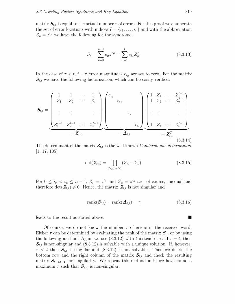
8.3 Decoding Basics: Syndrome and Key Equation 319
matrix St,t is equal to the actual number τ of errors. For this proof we enumeratethe set of error locations with indices I = {i1, . . . , iτ} and with the abbreviationZµ = ziµ we have the following for the syndrome:
Sr =
n−1∑µ=0
eµzrµ =
t∑µ=1
eiµZrµ. (8.3.13)
In the case of τ < t, t − τ error magnitudes eiµ are set to zero. For the matrixSt,t we have the following factorization, which can be easily verified:
St,t =
1 1 · · · 1Z1 Z2 · · · Zt
......
...
Zt−11 Zt−1
2 · · · Zt−1t
︸ ︷︷ ︸= Zt,t
·
ei1ei2
. . .
eit
︸ ︷︷ ︸= ∆t,t
·
1 Z1 · · · Zt−11
1 Z2 · · · Zt−12
......
...
1 Zt · · · Zt−1t
︸ ︷︷ ︸= Z T
t,t
.
(8.3.14)The determinant of the matrix Zt,t is the well known Vandermonde determinant[1, 17, 105]
det(Zt,t) =∏
t≥µ>ν≥1
(Zµ − Zν). (8.3.15)
For 0 ≤ iν < iµ ≤ n − 1, Zν = ziν and Zµ = ziµ are, of course, unequal andtherefore det(Zt,t) �= 0. Hence, the matrix Zt,t is not singular and
rank(St,t) = rank(∆t,t) = τ (8.3.16)
leads to the result as stated above. �
Of course, we do not know the number τ of errors in the received word.Either τ can be determined by evaluating the rank of the matrix St,t or by usingthe following method. Again we use (8.3.12) with t instead of τ . If τ = t, thenSt,t is non-singular and (8.3.12) is solvable with a unique solution. If, however,τ < t then St,t is singular and (8.3.12) is not solvable. Then we delete thebottom row and the right column of the matrix St,t and check the resultingmatrix St−1,t−1 for singularity. We repeat this method until we have found amaximum τ such that Sτ,τ is non-singular.
320 8. Reed-Solomon and Bose-Chaudhuri-Hocquenghem Codes
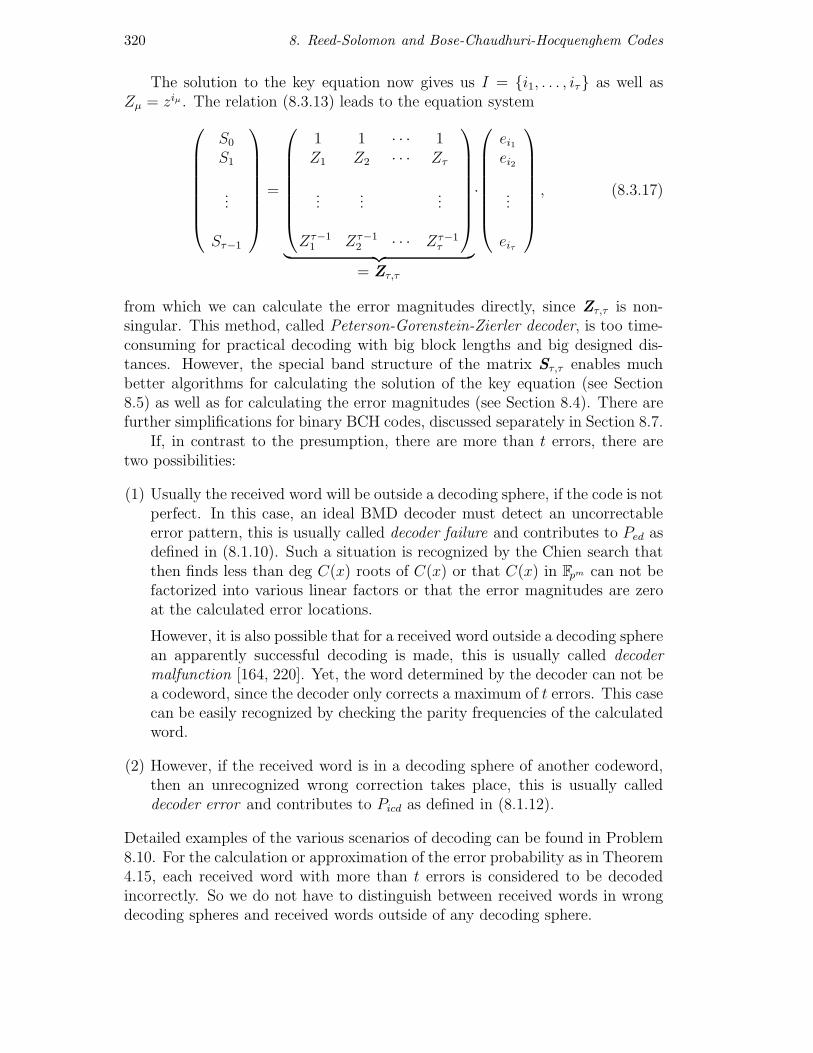
The solution to the key equation now gives us I = {i1, . . . , iτ} as well asZµ = ziµ . The relation (8.3.13) leads to the equation system
S0
S1
...
Sτ−1
=
1 1 · · · 1Z1 Z2 · · · Zτ
......
...
Zτ−11 Zτ−1
2 · · · Zτ−1τ
︸ ︷︷ ︸= Zτ,τ
·
ei1ei2
...
eiτ
, (8.3.17)
from which we can calculate the error magnitudes directly, since Zτ,τ is non-singular. This method, called Peterson-Gorenstein-Zierler decoder, is too time-consuming for practical decoding with big block lengths and big designed dis-tances. However, the special band structure of the matrix Sτ,τ enables muchbetter algorithms for calculating the solution of the key equation (see Section8.5) as well as for calculating the error magnitudes (see Section 8.4). There arefurther simplifications for binary BCH codes, discussed separately in Section 8.7.
If, in contrast to the presumption, there are more than t errors, there aretwo possibilities:
(1) Usually the received word will be outside a decoding sphere, if the code is notperfect. In this case, an ideal BMD decoder must detect an uncorrectableerror pattern, this is usually called decoder failure and contributes to Ped asdefined in (8.1.10). Such a situation is recognized by the Chien search thatthen finds less than deg C(x) roots of C(x) or that C(x) in Fpm can not befactorized into various linear factors or that the error magnitudes are zeroat the calculated error locations.
However, it is also possible that for a received word outside a decoding spherean apparently successful decoding is made, this is usually called decodermalfunction [164, 220]. Yet, the word determined by the decoder can not bea codeword, since the decoder only corrects a maximum of t errors. This casecan be easily recognized by checking the parity frequencies of the calculatedword.
(2) However, if the received word is in a decoding sphere of another codeword,then an unrecognized wrong correction takes place, this is usually calleddecoder error and contributes to Picd as defined in (8.1.12).
Detailed examples of the various scenarios of decoding can be found in Problem8.10. For the calculation or approximation of the error probability as in Theorem4.15, each received word with more than t errors is considered to be decodedincorrectly. So we do not have to distinguish between received words in wrongdecoding spheres and received words outside of any decoding sphere.
8.3 Decoding Basics: Syndrome and Key Equation 321
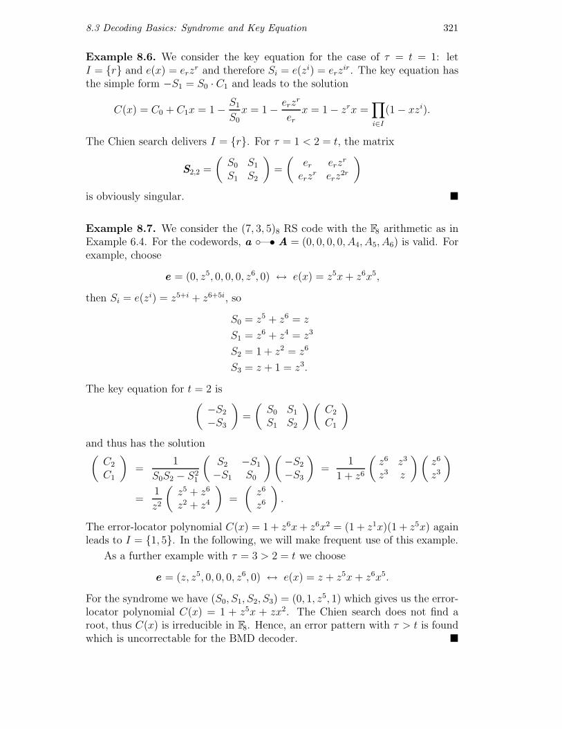
Example 8.6. We consider the key equation for the case of τ = t = 1: letI = {r} and e(x) = erz
r and therefore Si = e(zi) = erzir. The key equation has
the simple form −S1 = S0 · C1 and leads to the solution
C(x) = C0 + C1x = 1− S1
S0
x = 1− erzr
erx = 1− zrx =
∏i∈I
(1− xzi).
The Chien search delivers I = {r}. For τ = 1 < 2 = t, the matrix
S2,2 =
(S0 S1
S1 S2
)=
(er erz
r
erzr erz
2r
)is obviously singular. �
Example 8.7. We consider the (7, 3, 5)8 RS code with the F8 arithmetic as inExample 6.4. For the codewords, a ◦—• A = (0, 0, 0, 0, A4, A5, A6) is valid. Forexample, choose
e = (0, z5, 0, 0, 0, z6, 0) ↔ e(x) = z5x+ z6x5,
then Si = e(zi) = z5+i + z6+5i, so
S0 = z5 + z6 = z
S1 = z6 + z4 = z3
S2 = 1 + z2 = z6
S3 = z + 1 = z3.
The key equation for t = 2 is( −S2
−S3
)=
(S0 S1
S1 S2
)(C2
C1
)and thus has the solution(
C2
C1
)=
1
S0S2 − S21
(S2 −S1
−S1 S0
)( −S2
−S3
)=
1
1 + z6
(z6 z3
z3 z
)(z6
z3
)
=1
z2
(z5 + z6
z2 + z4
)=
(z6
z6
).
The error-locator polynomial C(x) = 1 + z6x+ z6x2 = (1 + z1x)(1 + z5x) againleads to I = {1, 5}. In the following, we will make frequent use of this example.
As a further example with τ = 3 > 2 = t we choose
e = (z, z5, 0, 0, 0, z6, 0) ↔ e(x) = z + z5x+ z6x5.
For the syndrome we have (S0, S1, S2, S3) = (0, 1, z5, 1) which gives us the error-locator polynomial C(x) = 1 + z5x + zx2. The Chien search does not find aroot, thus C(x) is irreducible in F8. Hence, an error pattern with τ > t is foundwhich is uncorrectable for the BMD decoder. �

322 8. Reed-Solomon and Bose-Chaudhuri-Hocquenghem Codes
8.4 Decoding Architectures
8.4.1 Frequency-Domain Error Correction
The error-locator polynomial C(x) and the set of unknown error locations I areknown after solving the key equation. Now, we have to determine the errormagnitudes e(x)◦—•E(x). According to (8.3.10),
Ei = −t∑
µ=1
CµEi−µ for i = 2t, . . . , n− 1 (8.4.1)
= function of (Ei−1, . . . , Ei−t).
This facilitates the principle of recursive extension: the start values are E0 =S0, . . . , E2t−1 = S2t−1. One after the other, E2t, . . . , En−1 are computed. Tech-nically, the recursive extension can be realized by a linear feedback shift register(LFSR, also called autoregressive filter) as shown in Figure 8.17. The length ofthe filter can be variable with τ or can be fixed to t. The start configuration isdefined by the t highest frequencies S2t−1, . . . , St of the syndrome. At the filteroutput, we have the values of E2t, . . . , En−1 sequentially.
–C1
.....Ei–1 Ei–t
–Ct
E
+
Ei
Figure 8.17. Computation of E(x) by recursive extension
Figure 8.18 shows the whole method of decoding in the frequency domain.Although the correction takes place in the time domain, the calculation of theerror magnitudes is performed in the frequency domain. Therefore we mustcompute the inverse Fourier transform of E(x), so that e(x) is available in thetime domain. However, we only have to determine the components which weredetected as being erroneous. To reduce the effort we will introduce a method inthe next subsection which can directly calculate the desired error magnitudes inthe time domain.
Example 8.8. Continuation of Example 8.7 with the (7, 3, 5)8 RS code. The
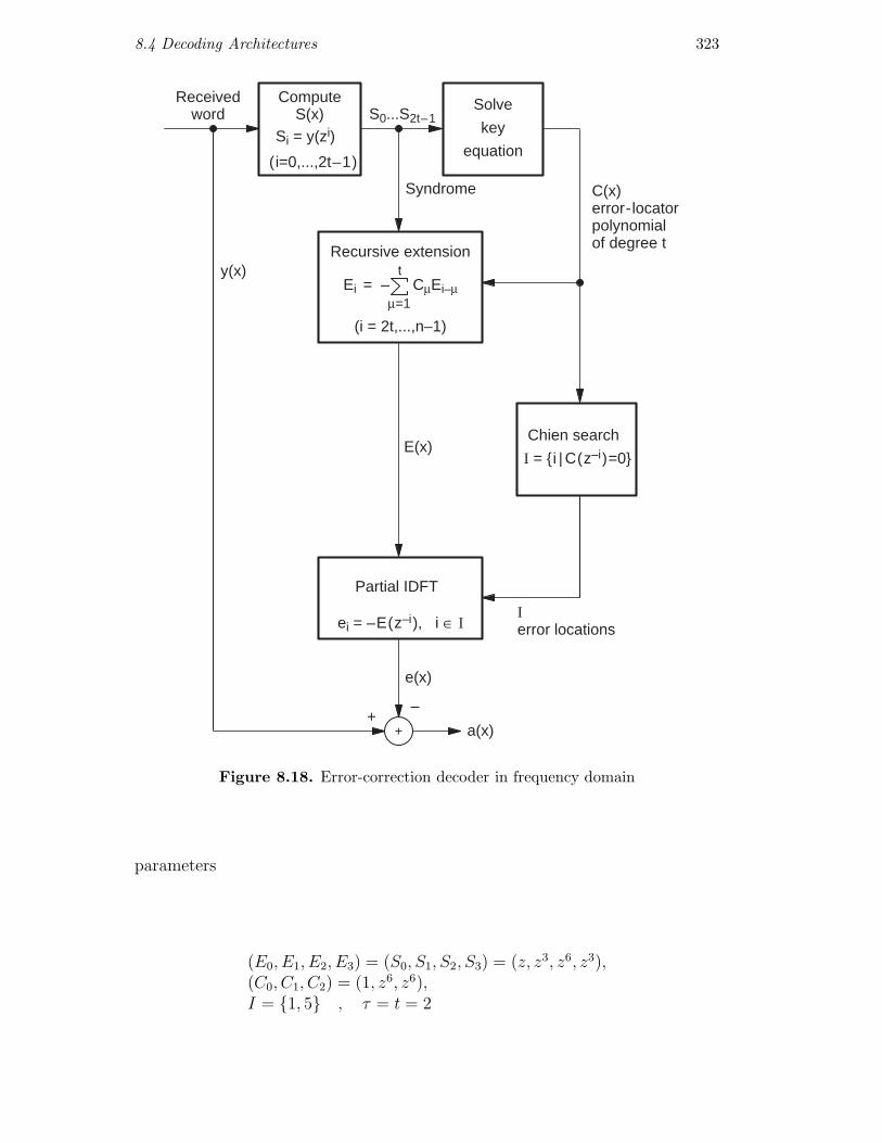
8.4 Decoding Architectures 323
Solve
key
equation
Partial IDFT
S0...S2t–1
Syndrome
Ierror locations
C(x)error-locatorpolynomialof degree t
Receivedword
t
µ=1Ei = – CµEi–µ
Recursive extension
(i = 2t,...,n–1)
ei = –E(z–i), i ∈ I
y(x)
E(x)
e(x)
+
ComputeS(x)
Si = y(zi)
(i=0,...,2t–1)
+–
a(x)
Chien search
I = {i | C(z–i)=0}
Figure 8.18. Error-correction decoder in frequency domain
parameters
(E0, E1, E2, E3) = (S0, S1, S2, S3) = (z, z3, z6, z3),(C0, C1, C2) = (1, z6, z6),I = {1, 5} , τ = t = 2

324 8. Reed-Solomon and Bose-Chaudhuri-Hocquenghem Codes
are already known. Recursive extension leads to
E4 = C1E3 + C2E2 = z6z3 + z6z6 = z3
E5 = C1E4 + C2E3 = z6z3 + z6z3 = 0
E6 = C1E5 + C2E4 = z60 + z6z3 = z2.
Finally,
E(x) = S0 + S1x+ S2x2 + S3x
3 + E4x4 + E5x
5 + E6x6
= z + z3x+ z6x2 + z3x3 + z3x4 + z2x6.
Since we have already determined that I = {1, 5}, all we need to do is calculatee1 and e5:
e1 = −E(z−1) = E(z6) = z + z2 + z4 + 1 + z6 + z3 = z5
e5 = −E(z−5) = E(z2) = z + z5 + z3 + z2 + z4 + 1 = z6.
Thus, the assumed error pattern e(x) = z5x+ z6x5 is the result. �
8.4.2 Time-Domain Error Correction
The objective now is to determine the error magnitudes at the desired positionsdirectly in the time domain without inverse Fourier transforms. As in the previ-ous subsection, the error-locator polynomial C(x) and the set of unknown errorlocations I are considered to be known after solving the key equation. Accordingto (8.3.9), a so-called error-evaluator polynomial T (x) exists with
C(x)E(x) = T (x)(xn − 1). (8.4.2)
T (x) does not directly show the error magnitudes, but the error magnitudes canbe calculated from T (x) as follows. For the degree of T (x),
deg T (x) = deg C(x)︸ ︷︷ ︸=τ
+deg E(x)︸ ︷︷ ︸≤n−1
− deg (xn − 1)︸ ︷︷ ︸=n
≤ τ − 1.
So T (x) kann be written as
T (x) = T0 + T1x+ · · ·+ Tτ−1xτ−1. (8.4.3)
The equation (8.4.2) is now written as
τ∑i=0
Cixi ·
2t−1∑i=0
Eixi
︸ ︷︷ ︸from x0 onwards
+ C(x)n−1∑i=2t
Eixi
︸ ︷︷ ︸from x2t onwards
= −T (x)︸ ︷︷ ︸until xτ−1
+ xnT (x)︸ ︷︷ ︸until xn
,
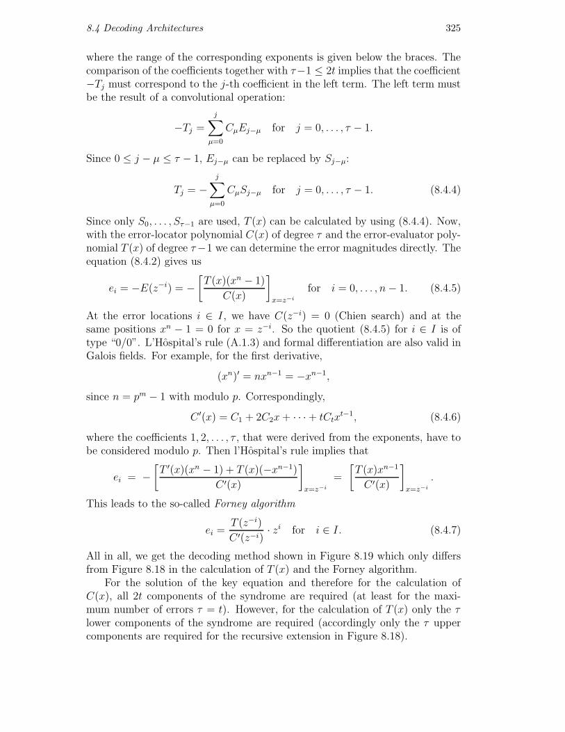
8.4 Decoding Architectures 325
where the range of the corresponding exponents is given below the braces. Thecomparison of the coefficients together with τ−1 ≤ 2t implies that the coefficient−Tj must correspond to the j-th coefficient in the left term. The left term mustbe the result of a convolutional operation:
−Tj =
j∑µ=0
CµEj−µ for j = 0, . . . , τ − 1.
Since 0 ≤ j − µ ≤ τ − 1, Ej−µ can be replaced by Sj−µ:
Tj = −j∑
µ=0
CµSj−µ for j = 0, . . . , τ − 1. (8.4.4)
Since only S0, . . . , Sτ−1 are used, T (x) can be calculated by using (8.4.4). Now,with the error-locator polynomial C(x) of degree τ and the error-evaluator poly-nomial T (x) of degree τ−1 we can determine the error magnitudes directly. Theequation (8.4.2) gives us
ei = −E(z−i) = −[T (x)(xn − 1)
C(x)
]x=z−i
for i = 0, . . . , n− 1. (8.4.5)
At the error locations i ∈ I, we have C(z−i) = 0 (Chien search) and at thesame positions xn − 1 = 0 for x = z−i. So the quotient (8.4.5) for i ∈ I is oftype “0/0”. L’Hospital’s rule (A.1.3) and formal differentiation are also valid inGalois fields. For example, for the first derivative,
(xn)′ = nxn−1 = −xn−1,
since n = pm − 1 with modulo p. Correspondingly,
C ′(x) = C1 + 2C2x+ · · ·+ tCtxt−1, (8.4.6)
where the coefficients 1, 2, . . . , τ , that were derived from the exponents, have tobe considered modulo p. Then l’Hospital’s rule implies that
ei = −[T ′(x)(xn − 1) + T (x)(−xn−1)
C ′(x)
]x=z−i
=
[T (x)xn−1
C ′(x)
]x=z−i
.
This leads to the so-called Forney algorithm
ei =T (z−i)C ′(z−i)
· zi for i ∈ I. (8.4.7)
All in all, we get the decoding method shown in Figure 8.19 which only differsfrom Figure 8.18 in the calculation of T (x) and the Forney algorithm.
For the solution of the key equation and therefore for the calculation ofC(x), all 2t components of the syndrome are required (at least for the maxi-mum number of errors τ = t). However, for the calculation of T (x) only the τlower components of the syndrome are required (accordingly only the τ uppercomponents are required for the recursive extension in Figure 8.18).
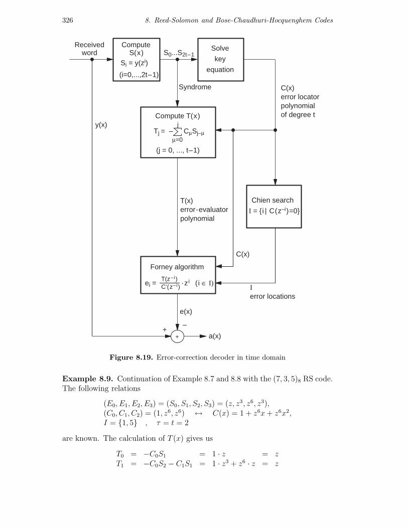
326 8. Reed-Solomon and Bose-Chaudhuri-Hocquenghem Codes
Solve
key
equation
Chien search
I = {i | C(z–i)=0}
Forney algorithm
S0...S2t–1
Syndrome
Ierror locations
C(x)error locatorpolynomialof degree t
Receivedword
j
µ=0Tj = – CµSj–µ
Compute T(x)
(j = 0, ..., t–1)
ei =
y(x)
T(x)error-evaluatorpolynomial
e(x)
+
ComputeS(x)
Si = y(zi)
(i=0,...,2t–1)
+–
a(x)
C(x)
(i ∈ I)T(z– i )C’(z– i ) · zi
Figure 8.19. Error-correction decoder in time domain
Example 8.9. Continuation of Example 8.7 and 8.8 with the (7, 3, 5)8 RS code.The following relations
(E0, E1, E2, E3) = (S0, S1, S2, S3) = (z, z3, z6, z3),(C0, C1, C2) = (1, z6, z6) ↔ C(x) = 1 + z6x+ z6x2,I = {1, 5} , τ = t = 2
are known. The calculation of T (x) gives us
T0 = −C0S1 = 1 · z = zT1 = −C0S2 − C1S1 = 1 · z3 + z6 · z = z

8.5 Solving the Key Equation 327
and thus T (x) = z + zx. Differentiation leads to C ′(x) = z6 + 2z6x = z6 mod 2.Furthermore, the Forney algorithm leads to
ei =T (z−i)C ′(z−i)
zi =z + z1−i
z6zi = z2+i + z2 =
{z5 i = 1z6 i = 5
}.
So the result is, once again, the assumed error pattern e(x) = z5x + z6x5. Fori �∈ I, the Forney algorithm does not give us the correct result ei = 0 but awrong, non-zero value, i.e., (8.4.7) is only valid for the error locations i ∈ I. �
8.5 Solving the Key Equation
8.5.1 The Berlekamp-Massey Algorithm
It was years after the discovery of RS and BCH codes that powerful algorithmswere developed for the solution of the key equation (8.3.11) or (8.3.12). Someof these algorithms are based on the Euclidean algorithm (found in 1975) andwill be introduced in the next subsection. A different method is the Berlekamp-Massey algorithm (BMA, found in 1968), which we examine here a withoutproof. Derivations of the BMA can be found in, e.g., [10, 17].
The equation (8.3.11) can be represented by a linear feedback shift regis-ter (LFSR) as shown in Figure 8.20. At the beginning (i = t) the register isinitialized with St−1, . . . , S0. One after the other the values St, . . . , S2t−1 arecreated at register input. However, to solve the key equation we do not haveto create the already known sequence of syndromes, but we are looking for thefilter coefficients for the sequence of syndromes, where the filter is to be of min-imum length. Thus solving the key equation is a problem of synthesizing anautoregressive filter.
–C1
.....Si–1 Si–t
–Ct
S0...S2t–1
+
Si
Figure 8.20. Generierung des Syndroms durch das Fehlerstellenpolynom
Figure 8.21 shows the Berlekamp-Massey algorithm. The input is the syn-drome (S0, . . . , S2t−1) and the output is the error-locator polynomial C(x) =C(j)(x) with the stop condition j = 2t.

328 8. Reed-Solomon and Bose-Chaudhuri-Hocquenghem Codes
2e > j ?
Initialize:
error-locator polynomialauxiliary polynomialcounters
C(0)(x) = 1B(0)(x) = 0
e = 0j = 0
k = 0
e
µ=1∆j = Sj + Cµ Sj–µ = 0 ?
(j)
C(j+1)(x) = C(j)(x) – ∆jxkB(j)(x) C(j+1)(x) = C(j)(x)
j ≥ 2t ?
B(j+1)(x) = ∆j C(j)(x) B(j+1)(x) = B(j)(x)
k = k+1
j = j+1
Stop
yes
yes
yesno
no
no
–1
e = j+1–ek = 1
Figure 8.21. The Berlekamp-Massey algorithm
We present only a short descriptive explanation of the BMA. The countere runs through the length of the filter and j runs through the length of the se-quence of syndromes synthesized up until now. At ∆j = 0? a check is made tosee whether we can create the next Sj using the current C(j)(x) and the currentlength e. If not then the filter coefficients are modified. Then at 2eold ≤ j thefilter is extended: enew = j+1− eold ≥ eold+1. Furthermore the auxiliary poly-

8.5 Solving the Key Equation 329
nomial B(x) is used as a temporary buffer for the last-but-one C(x). Withoutthe extension of the filter, B(x) remains unchanged. Finally, j is incrementedin any case. During the whole algorithm, j ≥ e and j ≤ 2t− 1 are always validso that at ∆j = 0? only the known syndrome values S0, . . . , S2t−1 are required.
An error pattern which is uncorrectable for the BMD decoder is detected,if, after the termination of the BMA, the degree of the calculated polynomialC(x) is unequal to e or if deg C(x) = e > t or if the Chien search finds fewerthan deg C(x) roots in the polynomial C(x).
Example 8.10. Continuation of Example 8.7 with the (7, 3, 5)8 RS code andt = 2 and l = 0. For the syndrome of the error pattern e(x) = z5x + z6x5,(S0, S1, S2, S3) = (z, z3, z6, z3). The BMA works as follows:
e k j ∆j C(j+1)(x) 2e > j B(j+1)(x)0 0 0 z 1 no z6
1 1 1 z3 1 + z2x yes z6
1 2 2 z 1 + z2x+ x2 no z6 + zx2 1 3 z 1 + z6x+ z6x2 yes z6 + zx2 2 4 Stop
The comparison with Example 8.7 shows that the result C(x) = C(4)(x) =1 + z6x+ z6x2 is correct. �
In Table 8.6, the necessary addition-and-multiplication operations for thedecoding of RS codes are approximately summarized. The BMA reduces theeffort for solving the key equation from t3 to t2 and is therefore unproblematic.The error correction in the time domain is less time-consuming than in thefrequency domain. The biggest effort is caused by the partial transformationsfor calculating the syndrome, by the Chien search and by the encoder. However,the effort can be reduced by using fast algorithms [17, 18] as well as using varioussymmetries which exist in some cases. Many hints and ideas for implementingthe algorithms are given in [79] and especially in [145]. For binary BCH codes,there are enormous simplifications which will be discussed in Section 8.7.
The equation (8.3.9) is valid regardless of where the parity frequencies aresituated. So if, instead of S0, . . . , S2t−1, the values Sl, . . . , Sl+2t−1 are known,then we only have to shift the indices into the range of 0, . . . , 2t − 1. The keyequation (8.3.11) takes on the form
Si +
τ∑µ=1
CµSj−µ = 0 for i = l + τ, . . . , l + 2τ − 1 (8.5.1)
and the switch condition on ∆j in the BMA is to be changed into
∆j = Sj+l +e∑
µ=1
C(j)µ Sj−µ+l = 0 ? (8.5.2)
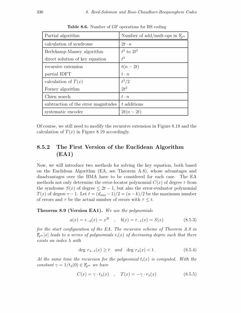
330 8. Reed-Solomon and Bose-Chaudhuri-Hocquenghem Codes
Table 8.6. Number of GF operations for RS coding
Partial algorithm Number of add/mult-ops in Fpm
calculation of syndrome 2t · nBerlekamp-Massey algorithm t2 to 2t2
direct solution of key equation t3
recursive extension t(n− 2t)
partial IDFT t · ncalculation of T (x) t2/2
Forney algorithm 2t2
Chien search t · nsubtraction of the error magnitudes t additions
systematic encoder 2t(n− 2t)
Of course, we still need to modify the recursive extension in Figure 8.18 and thecalculation of T (x) in Figure 8.19 accordingly.
8.5.2 The First Version of the Euclidean Algorithm
(EA1)
Now, we will introduce two methods for solving the key equation, both basedon the Euclidean Algorithm (EA, see Theorem A.8), whose advantages anddisadvantages over the BMA have to be considered for each case. The EAmethods not only determine the error-locator polynomial C(x) of degree τ fromthe syndrome S(x) of degree ≤ 2t − 1, but also the error-evaluator polynomialT (x) of degree τ −1. Let t = (dmin−1)/2 = (n−k)/2 be the maximum numberof errors and τ be the actual number of errors with τ ≤ t.
Theorem 8.9 (Version EA1). We use the polynomials
a(x) = r−2(x) = x2t , b(x) = r−1(x) = S(x) (8.5.3)
for the start configuration of the EA. The recursive scheme of Theorem A.8 inFpm [x] leads to a series of polynomials ri(x) of decreasing degree such that thereexists an index λ with
deg rλ−1(x) ≥ t and deg rλ(x) < t. (8.5.4)
At the same time the recursion for the polynomial ti(x) is computed. With theconstant γ = 1/tλ(0) ∈ Fpm we have
C(x) = γ · tλ(x) , T (x) = −γ · rλ(x) (8.5.5)

8.5 Solving the Key Equation 331
for the error-locator and the error-evaluator polynomial.
Proof. Although the recursion for the polynomial si(x) is used for this proof,it does not have to be calculated in practical applications of the algorithm.According to (A.7.6), the recursive polynomials are linked as
rλ(x) = sλ(x)x2t + tλ(x)S(x). (8.5.6)
According to (A.7.16),
deg tλ(x) = deg a(x)︸ ︷︷ ︸=2t
− deg rλ−1(x)︸ ︷︷ ︸≥t
≤ t.
The main equation (8.4.2) can be written as
(xn − 1)T (x) = C(x)E(x) = C(x)
(S(x) +
n−1∑i=2t
Eixi
)
and with an appropriate polynomial L(x) we then have
−T (x) = C(x)S(x) + x2tL(x). (8.5.7)
The multiplication of (8.5.6) by C(x) together with (8.5.7) leads to
C(x)rλ(x)︸ ︷︷ ︸deg<t+τ
= C(x)sλ(x)x2t + C(x)S(x)tλ(x)
= −T (x)tλ(x)︸ ︷︷ ︸deg<τ+t
+(C(x)sλ(x)− L(x)tλ(x)
)x2t︸ ︷︷ ︸
deg≥2t
.
Comparing the degrees gives us
C(x)sλ(x) = L(x)tλ(x), (8.5.8)
C(x)rλ(x) = −T (x)tλ(x). (8.5.9)
The error-locator polynomial C(x) has the roots z−i for i ∈ I. Since these zerosare only singular, C ′(z−i) �= 0 must be valid for the first derivative and theForney algorithm (8.4.7) implies that T (z−i) �= 0 for i ∈ I. Thus, accordingto (8.5.9), C(x) has to be a factor of tλ(x), hence, there exists a polynomialβ(x) = tλ(x)/C(x). Trivially, β(x) is a factor of tλ(x) and, according to (8.5.8),β(x) is also a factor of sλ(x). However, according to (A.7.10), sλ(x) and tλ(x)do not have a common divisor, thus β(x) = γ−1 is a constant that is determinedfrom γ−1 = β(0) = tλ(0)/C(0) = tλ(0). Thus C(x) = γ · tλ(x) is obvious andT (x) = −γ · rλ(x) is implied by (8.5.9). �

332 8. Reed-Solomon and Bose-Chaudhuri-Hocquenghem Codes
Example 8.11. As in Example 8.7, we will consider the (7, 3, 5)8 RS code witht = 2 and the error pattern e(x) = z5x+z6x5 with S(x) = z+z3x+z6x2+z3x3.The EA leads to the recursive scheme
x4︸︷︷︸r−2(x)
= z4x︸︷︷︸α0(x)
· (z3x3 + z6x2 + z3x+ z)︸ ︷︷ ︸r−1(x)
+ (z3x3 + x2 + z5x)︸ ︷︷ ︸r0(x)
(z3x3 + z6x2 + z3x+ z)︸ ︷︷ ︸r−1(x)
= 1︸︷︷︸α1(x)
· (z3x3 + x2 + z5x)︸ ︷︷ ︸r0(x)
+ (z2x2 + z2x+ z)︸ ︷︷ ︸r1(x)
(z3x3 + x2 + z5x)︸ ︷︷ ︸r0(x)
= (zx+ z6)︸ ︷︷ ︸α2(x)
· (z2x2 + z2x+ z)︸ ︷︷ ︸r1(x)
+ (x+ 1)︸ ︷︷ ︸r2(x)
.
Thus λ = 2. According to (A.7.3), the ti(x) recursion is
t0(x) = t−2(x)− α0(x)t−1(x) = z4xt1(x) = t−1(x)− α1(x)t0(x) = 1 + z4xt2(x) = t0(x)− α2(x)t1(x) = z6 + z5x+ z5x2.
Thus γ = 1/tλ(0) = z and, according to Theorem 8.9, C(x) = zt2(x) = 1 +z6x + z6x2 as well as T (x) = −zr2(x) = z + zx, which are equal to the resultsof Examples 8.7 and 8.9. �
8.5.3 The Second Version of the Euclidean Algorithm
(EA2)
An alternative application of the EA for determining C(x) and T (x) is based onthe complementary error-locator polynomial of degree n− |I| = n− τ :
C∗(x) =∏i�∈I
(1− xzi). (8.5.10)
While keeping {z0, . . . , zn−1} = {z−0, . . . , z−(n−1)} in mind, according to(7.2.13),
C(x)C∗(x) =n−1∏i=0
(1− xzi) =
(n−1∏i=0
(−zi)
)·(n−1∏i=0
(x− z−i)
)
= ∆ · (xn − 1) with ∆ ∈ Fpm. (8.5.11)
For i ∈ I, C∗(x) has the roots z−i and ei = −E(z−i) = 0. So C∗(x) splits upinto linear factors which are also linear factors of E(x), thus C∗(x) is a factor ofxn − 1 as well as of E(x). Since C(x) is to have a minimum degree and C∗(x)is to have a maximum degree,
C∗(x) = GCD(E(x), xn − 1
). (8.5.12)

8.5 Solving the Key Equation 333
Now, we perform a cyclic shift of n − 2t positions to the right on E(x), suchthat the known syndromes are in the higher frequencies and the unknown errormagnitudes are in the lower frequencies:
Es(x) = Rxn−1[xn−2tE(x)] ↔ (E2t, . . . , En−1, S0, . . . , S2t−1). (8.5.13)
According to Theorem 7.8, this implies a multiplication for es(x)◦—•Es(x) inthe time domain, hence es,i = ei · z−i(n−2t) for the coefficients of es(x). Since theerror magnitudes do not move, E(x) and Es(x) have the same roots, thus
C∗(x) = GCD(Es(x), x
n − 1). (8.5.14)
Corresponding to (8.4.2), there is a representation
C(x)Es(x) = Ts(x)(xn − 1), (8.5.15)
where Ts(x) is the error-evaluator polynomial for es(x).
Theorem 8.10 (Version EA2). We choose the polynomials
a(x) = r−2(x) = xn − 1 , b(x) = r−1(x) = Es(x) (8.5.16)
for the start configuration of the EA. The recursive scheme of Theorem A.8 inFpm [x] leads to a series of polynomials ri(x) of decreasing degree such that thereexists a minimum index λ with
deg rλ+1(x) < n− t. (8.5.17)
At the same time, the recursions for the polynomials si(x) and ti(x) are com-puted. With the constant γ = 1/tλ+1(0) ∈ Fpm we have
C(x) = γ · tλ+1(x) , Ts(x) = −γ · sλ+1(x) (8.5.18)
for the error-locator and the error-evaluator polynomial.
Proof. According to Theorem A.8, there exists an index λ with
rλ(x) = GCD(xn − 1, Es(x)) = C∗(x) and rλ+1(x) = 0.
So, for i ≤ λ, deg ri(x) ≥ deg rλ(x) = n−τ ≥ n− t and for i ≥ λ+1, ri(x) = 0.According to (A.7.5),
(−1)λtλ+1(x) =xn − 1
GCD(xn − 1, Es(x))=
xn − 1
C∗(x)= ∆−1C(x),
−(−1)λsλ+1(x) =Es(x)
GCD(xn − 1, Es(x))=
Es(x)
C∗(x)= ∆−1Ts(x),

334 8. Reed-Solomon and Bose-Chaudhuri-Hocquenghem Codes
where (8.5.11) implies the right hand side of the equalities. The polynomialC(x) = ∆(−1)λtλ+1(x) with x = 0 implies that γ = ∆(−1)λ = 1/tλ+1(0). Sothe proof is complete. Finally, (A.7.15) and (A.7.16) can be used to verify thecorrect degrees of C(x) and Ts(x). �
Because of the special relation of the degrees, the EA can actually be per-formed, although only the upper 2t powers of Es(x) are known. Here is anexample that makes this quite clear:
Example 8.12. We make the same presumptions as for Example 8.11 with theerror pattern e(x) = z5x+ z6x5. The shift in the frequency domain leads to
es(x) = z5−1·3x+ z6−5·3x5 = z2x+ z5x5
in the time domain. In fact, we do not know the polynomials es(x) or Es(x)completely but only
Es(x) = (E4, E5, E6, S0, S1, S2, S3) = (, z, z3, z6, z3),
where the coefficients E4, E5, E6 are unknown. With the start configuration ofr−2(x) = xn − 1 = x7 + 1 and r−1(x) = Es(x) the EA gives us the recursivescheme
(x7 + 1)︸ ︷︷ ︸r−2(x)
= (z4x+ 1)︸ ︷︷ ︸α0(x)
· (z3x6 + z6x5 + z3x4 + zx3 + . . .)︸ ︷︷ ︸r−1(x)
+ (z2x5 + z2x4 + . . .)︸ ︷︷ ︸r0(x)
(z3x6 + z6x5 + z3x4 + zx3 + . . .)︸ ︷︷ ︸r−1(x)
= (zx + z2)︸ ︷︷ ︸α1(x)
· (z2x5 + z2x4 + . . .)︸ ︷︷ ︸r0(x)
+ (x4 . . .)︸ ︷︷ ︸r1(x)
.
With deg r1(x) < n− t = 5 we have λ = 0. So inevitably r1(x) = 0. Accordingto (A.7.3),
t0(x) = t−2(x)− α0(x)t−1(x) = z4x+ 1
t1(x) = t−1(x)− α1(x)t0(x) = 1 + (zx+ z2)(z4x+ 1) = z5x2 + z5x+ z6
for the ti(x) recursion, and
s0(x) = s−2(x)− α0(x)s−1(x) = 1
s1(x) = s−1(x)− α1(x)s0(x) = zx+ z2
for the the si(x)-recursion. The polynomials of (8.5.18) with γ = 1/t1(0) = zgive us our usual results C(x) = zt1(x) = 1 + z6x + z6x2 as well as Ts(x) =zs1(x) = z3 + zx. The Forney algorithm with
es,i =Ts(z
−i)C ′(z−i)
=z3 + z2−i
z6zi =
{z2 i = 1z5 i = 5
}implies the correct result for es(x). �

8.6 Error-and-Erasure Decoding with RS Codes 335
8.6 Error-and-Erasure Decoding with RS
Codes
8.6.1 Overview and Decoding Capability
We presuppose a q-ary symmetric channel with erasures as a generalization ofthe BSEC of Figure 1.4:
Ain = Fq , Aout = Fq ∪ {?}. (8.6.1)
The demodulator decides on y = ? (erasure), if the decision on a specific y ∈ Fqwas too unreliable. The advantage of this method is that the correction of suchan erasure (position known, transmitted symbol unknown) only requires oneparity-check symbol, whereas to correct an error (position unknown, transmit-ted symbol and error symbol unknown) two parity-check symbols are required.Formally, the received word as an extension to (8.3.1) is described by
y = a + e + v , (8.6.2)
where a ∈ Fnq is the codeword, e ∈ Fn
q is the error word and v ∈ {0, ?}n isthe erasure word. As the components yi and vi can take on the value ?, thearithmetic operations between ? and b ∈ Fq are formally defined as
b+? = ? , b·? = ? fur b �= 0 , 0·? = 0. (8.6.3)
In addition to the set of unknown error locations I and the error-locator poly-nomial C(x), we will now introduce the set of known erasure locations Iv andthe erasure-locator polynomial Cv(x):
I = {i | ei �= 0} , C(x) =∏i∈I
(1− xzi), (8.6.4)
Iv = {i | vi = ?} , Cv(x) =∏i∈Iv
(1− xzi). (8.6.5)
Per definition, an erasure is not considered to be an error, thus I and Iv aredisjoint. Of course, I and C(x) are unknown, whereas Iv and Cv(x) are known.Let τ = |I| = deg C(x) be the unknown number of errors and τv = |Iv| =deg Cv(x) be the known number of erasures. The decoding method describedbelow proves the following theorem.
Theorem 8.11 (Error-and-Erasure Decoding). An (n, n − 2t, 2t+ 1)q RScode corrects τ errors and τv erasures, if
2τ + τv ≤ 2t = dmin − 1 = n− k. (8.6.6)

336 8. Reed-Solomon and Bose-Chaudhuri-Hocquenghem Codes
For τ = 0 and τv = n − k, this corresponds to the statement of Theorem 4.8,because k arbitrary correct positions in the codeword uniquely determine thewhole codeword. The calculation of the error probability for the error-and-erasure correction will be covered in Theorem 11.1?.
The decoding is performed in two major steps. The first step completelyeliminates the influence of erasures by using a trick, so that the usual methodsof error correction can be applied. Then the second step corrects the erasures.
8.6.2 First Step: Error Correction
For i ∈ Iv, cv,i = −Cv(z−i) = 0 and for i �∈ Iv, vi = 0. Thus vicv,i = 0 for
0 ≤ i ≤ n− 1. The representation (8.6.2) implies that
yicv,i︸︷︷︸yi
= aicv,i︸ ︷︷ ︸ai
+ eicv,i︸︷︷︸ei
+ vicv,i︸︷︷︸0
. (8.6.7)
Since I and Iv are disjoint, the combination ei �= 0 and cv,i = 0 is impossible,thus ei = 0 is equivalent to ei = 0. Therefore the influence of the erasures iscompletely eliminated in y = a + e, and the error locations remain unchanged.However, the error magnitudes have been modified and the syndrome is reducedby τv components, as we will see shortly. According to Theorem 7.8, the trans-formation of (8.6.7) into the frequency domain leads to
Rxn−1[−Y (x)Cv(x)]︸ ︷︷ ︸Y (x)
= Rxn−1[−A(x)Cv(x)]︸ ︷︷ ︸A(x)
+Rxn−1[−E(x)Cv(x)]︸ ︷︷ ︸E(x)
. (8.6.8)
The product A(x)Cv(x) has the degree ≤ (n − 1) + τv, so that the upper τvpowers are added to the lower powers by the modulo (xn − 1) operation:
A = (0, . . . , 0︸ ︷︷ ︸2t zeros
, A2t, . . . , An−1︸ ︷︷ ︸n− 2t positions
),
A = (A0, . . . , Aτv−1︸ ︷︷ ︸τv positions
, 0, . . . , 0︸ ︷︷ ︸2t−τv zeros
, A2t, . . . , An−1︸ ︷︷ ︸n−2t positions
). (8.6.9)
Thus, for the syndrome, we can only use the 2t− τv positions of the error word,which are left unchanged by the codeword, thus S = (Eτv , . . . , E2t−1) is the newsyndrome. According to the presupposition (8.6.6), 2τ ≤ 2t− τv, and thereforeτ errors are correctable. For solving the key equation, we now have to note that,according to (8.3.10) or (8.5.2),
Ei +τ∑
µ=1
CµEi−µ = 0 for i = τv + τ, . . . , τv + 2τ − 1. (8.6.10)

8.6 Error-and-Erasure Decoding with RS Codes 337
Since all indices of Ei are within the range of τv, . . . , τv +2t− 1, Ei correspondsto the known syndrome Si. So, the τ equations of (8.6.10) completely determinethe τ unknowns C1, . . . , Cτ .
So now the error-locator polynomial C(x) is given. The error correctioncan be performed similarly to Subsection 8.4.1 or 8.4.2 or the errors can beinterpreted as erasures for the decoding to come, since their locations are nowknown. Therefore, from now on we will only need to consider the correction oferasures.
8.6.3 Second Step: Erasure Correction
After the first step, we can now assume that the received word is superimposedby erasures only, so for y = a + v ,
Iv = {i | vi = ?} , Cv(x) =∏i∈Iv
(1− xzi),
τv = |Iv| = deg Cv(x) ≤ 2t,(8.6.11)
where Iv, Cv(x) and τv known. In the frequency domain,
Y = A+V = (V0, . . . , V2t−1, A2t + V2t, . . . , An−1 + Vn−1). (8.6.12)
For the actual calculation, yi is set to zero at the erasure locations. Accordingto the first step, vicv,i = 0 for 0 ≤ i ≤ n− 1, and according to Theorem 7.8, wehave our usual implication of
Rxn−1[Cv(x)V (x)] = 0, (8.6.13)
or equivalently expressed by the cyclic convolution,
τv∑µ=0
Cv,µV(i−µ) mod n = 0 fur i = 0, . . . , n− 1. (8.6.14)
So a recursive extension of the components V2t, . . . , Vn−1 is possible from theknown values V0, . . . , V2t−1 with
Vi = −τv∑µ=1
Cv,µVi−µ for i = n− 2t, . . . , n− 1 (8.6.15)
= function of (Vi−1, . . . , Vi−τv).
With the inverse transform vi = −V (z−i), erasure correction can be performedin the frequency domain. An alternative is the erasure correction in the timedomain: according to (8.6.13), there exists an error-evaluator polynomial Tv(x)of degree ≤ τv − 1 with
Cv(x)V (x) = Tv(x)(xn − 1). (8.6.16)

338 8. Reed-Solomon and Bose-Chaudhuri-Hocquenghem Codes
Then, corresponding to (8.4.4),
Tv,j = −j∑
µ=0
Cv,µVj−µ for j = 0, . . . , τv − 1 (8.6.17)
and the Forney algorithm is
vi =Tv(z
−i)C ′v(z
−i)· zi for i ∈ Iv. (8.6.18)
Example 8.13. As in Examples 8.7 to 8.12, we again consider the (7, 3, 5)8 RScode with t = 2 and
a = (z5, z3, z2, z, z4, z6, 1) ◦—• (0, 0, 0, 0, 1, z, z2) unknown,e = (0, 0, 0, 0, 0, z5, 0) d.h. τ = 1, I = {5} unknown,v = (0, ?, 0, 0, ?, 0, 0) d.h. τv = 2, Iv = {1, 4} known.
For the received word y = (z5, ?, z2, z, ?, z6 + z5 = z, 1), the receiver knows theerasure-locator polynomial Cv(x) = (1− xz1)(1− xz4) = 1 + z2x+ z5x2.
Step 1: error correction or location of errors. The equation cv,i =−Cv(z
−i) = 1 + z2−i + z5−2i implies that cv = (z, 0, z, 1, 0, z3, z3). Thus thereceiver can create y = (z6, 0, z3, z, 0, z4, z3), according to (7.10.7). Since
Y = (Y0, Y1, E2, E3, Y4, Y5, Y6)
we only need to determine Yi = y(zi) = Ei for i = 2, 3:
E2 = Y2 = y(z2) = z6 + z3(z2)2 + z(z2)3 + z4(z2)5 + z3(z2)6 = z4
E3 = Y3 = y(z3) = z6 + z3(z3)2 + z(z3)3 + z4(z3)5 + z3(z3)6 = z2.
The key equation (8.6.10) is E3 + C1E2 = 0 implying that C1 = −E3/E2 = z5.Thus C(x) = C0 + C1x = 1− xz5 which implies the correct result for I = {5}.From now on we will treat this located error as an erasure.
Step 2: erasure correction for Iv = {1, 4, 5} with τv = 3. The received wordis y = (z5, ?, z2, z, ?, ?, 1) and the error-locator polynomial is
Cv(x) = (1− xz1)(1− xz4)(1− xz5) = 1 + z3x+ z4x2 + z3x3.
With 0 for ?, Yi = y(zi) = z5 + z2+2i + z1+3i + z6i implies that
Y = (0, z, z2, 0, z, 0, z3) = (V0, V1, V2, V3, Y4, Y5, Y6).
The recursive extension with Vi = Cv,1Vi−1 + Cv,2Vi−2 + Cv,3Vi−3 as in (8.6.15)leads to
V4 = z3V3 + z4V2 + z3V1 = 0 + z6 + z4 = z3
V5 = z3V4 + z4V3 + z3V2 = z6 + 0 + z5 = zV6 = z3V5 + z4V4 + z3V3 = z4 + 1 + 0 = z5.
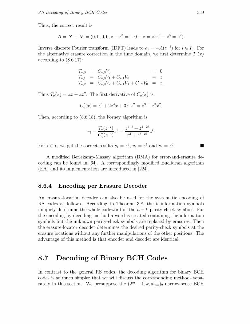
8.7 Decoding of Binary BCH Codes 339
Thus, the correct result is
A = Y −V = (0, 0, 0, 0, z − z3 = 1, 0− z = z, z3 − z5 = z2).
Inverse discrete Fourier transform (IDFT) leads to ai = −A(z−i) for i ∈ Iv. Forthe alternative erasure correction in the time domain, we first determine Tv(x)according to (8.6.17):
Tv,0 = Cv,0V0 = 0Tv,1 = Cv,0V1 + Cv,1V0 = zTv,2 = Cv,0V2 + Cv,1V1 + Cv,2V0 = z.
Thus Tv(x) = zx+ zx2. The first derivative of Cv(x) is
C ′v(x) = z3 + 2z4x+ 3z3x2 = z3 + z3x2.
Then, according to (8.6.18), the Forney algorithm is
vi =Tv(z
−i)C ′v(z
−i)zi =
z1−i + z1−2i
z3 + z3−2izi.
For i ∈ Iv we get the correct results v1 = z3, v4 = z4 and v5 = z6. �
A modified Berlekamp-Massey algorithm (BMA) for error-and-erasure de-coding can be found in [64]. A correspondingly modified Euclidean algorithm(EA) and its implementation are introduced in [224].
8.6.4 Encoding per Erasure Decoder
An erasure-location decoder can also be used for the systematic encoding ofRS codes as follows. According to Theorem 3.8, the k information symbolsuniquely determine the whole codeword or the n− k parity-check symbols. Forthe encoding-by-decoding method a word is created containing the informationsymbols but the unknown parity-check symbols are replaced by erasures. Thenthe erasure-locator decoder determines the desired parity-check symbols at theerasure locations without any further manipulations of the other positions. Theadvantage of this method is that encoder and decoder are identical.
8.7 Decoding of Binary BCH Codes
In contrast to the general RS codes, the decoding algorithm for binary BCHcodes is so much simpler that we will discuss the corresponding methods sepa-rately in this section. We presuppose the (2m − 1, k, dmin)2 narrow-sense BCH
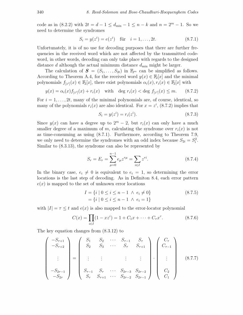
340 8. Reed-Solomon and Bose-Chaudhuri-Hocquenghem Codes
code as in (8.2.2) with 2t = d − 1 ≤ dmin − 1 ≤ n − k and n = 2m − 1. So weneed to determine the syndromes
Si = y(zi) = e(zi) fur i = 1, . . . , 2t. (8.7.1)
Unfortunately, it is of no use for decoding purposes that there are further fre-quencies in the received word which are not affected by the transmitted code-word, in other words, decoding can only take place with regards to the designeddistance d although the actual minimum distance dmin might be larger.
The calculation of S = (S1, . . . , S2t) in F2m can be simplified as follows.According to Theorem A.4, for the received word y(x) ∈ F2[x] and the minimalpolynomials f[zi](x) ∈ F2[x], there exist polynomials αi(x), ri(x) ∈ F2[x] with
y(x) = αi(x)f[zi](x) + ri(x) with deg ri(x) < deg f[zi](x) ≤ m. (8.7.2)
For i = 1, . . . , 2t, many of the minimal polynomials are, of course, identical, somany of the polynomials ri(x) are also identical. For x = zi, (8.7.2) implies that
Si = y(zi) = ri(zi). (8.7.3)
Since y(x) can have a degree up to 2m − 2, but ri(x) can only have a muchsmaller degree of a maximum of m, calculating the syndrome over ri(x) is notas time-consuming as using (8.7.1). Furthermore, according to Theorem 7.9,we only need to determine the syndromes with an odd index because S2i = S2
i .Similar to (8.3.13), the syndrome can also be represented by
Sr = Er =
n−1∑µ=0
eµzrµ =
∑i∈I
zri. (8.7.4)
In the binary case, ei �= 0 is equivalent to ei = 1, so determining the errorlocations is the last step of decoding. As in Definiton 8.4, each error patterne(x) is mapped to the set of unknown error locations
I = {i | 0 ≤ i ≤ n− 1 ∧ ei �= 0} (8.7.5)
= {i | 0 ≤ i ≤ n− 1 ∧ ei = 1}with |I| = τ ≤ t and e(x) is also mapped to the error-locator polynomial
C(x) =∏i∈I
(1− xzi) = 1 + C1x+ · · ·+ Cτxτ . (8.7.6)
The key equation changes from (8.3.12) to
−Sτ+1
−Sτ+2
...
−S2τ−1
−S2τ
=
S1 S2 · · · Sτ−1 SτS2 S3 · · · Sτ Sτ+1
......
......
Sτ−1 Sτ · · · S2τ−3 S2τ−2
Sτ Sτ+1 · · · S2τ−2 S2τ−1
·
Cτ
Cτ−1
...
C2
C1
(8.7.7)
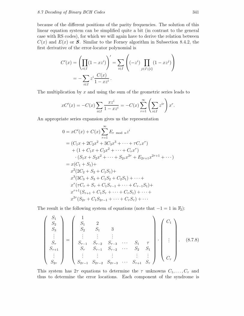
8.7 Decoding of Binary BCH Codes 341
because of the different positions of the parity frequencies. The solution of thislinear equation system can be simplified quite a bit (in contrast to the generalcase with RS codes), for which we will again have to derive the relation betweenC(x) and E(x) or S . Similar to the Forney algorithm in Subsection 8.4.2, thefirst derivative of the error-locator polynomial is
C ′(x) =
(∏i∈I
(1− xzi)
)′
=∑i∈I
(−zi)
∏j∈I\{i}
(1− xzj)
= −∑i∈I
ziC(x)
1− xzi.
The multiplication by x and using the sum of the geometric series leads to
xC ′(x) = −C(x)∑i∈I
xzi
1− xzi= −C(x)
∞∑r=1
(∑i∈I
zir
)xr.
An appropriate series expansion gives us the representation
0 = xC ′(x) + C(x)
∞∑r=1
Er mod nzi
= (C1x+ 2C2x2 + 3C3x
3 + · · ·+ τCτxτ )
+ (1 + C1x+ C2x2 + · · ·+ Cτx
τ )
· (S1x+ S2x2 + · · ·+ S2τx
2τ + E2τ+1x2τ+1 + · · · )
= x(C1 + S1)+
x2(2C2 + S2 + C1S1)+
x3(3C3 + S3 + C1S2 + C2S1) + · · ·+xτ (τCτ + Sτ + C1Sτ−1 + · · ·+ Cτ−1S1)+
xτ+1(Sτ+1 + C1Sτ + · · ·+ CτS1) + · · ·+x2τ (S2τ + C1S2τ−1 + · · ·+ CτSτ ) + · · ·
The result is the following system of equations (note that −1 = 1 in F2):
S1
S2
S3...SτSτ+1...
S2τ
=
1S1 2S2 S1 3...
......
Sτ−1 Sτ−2 Sτ−3 · · · S1 τSτ Sτ−1 Sτ−2 · · · S2 S1...
......
......
S2τ−1 S2τ−2 S2τ−3 · · · Sτ+1 Sτ
·
C1
...
Cτ
. (8.7.8)
This system has 2τ equations to determine the τ unknowns C1, . . . , Cτ andthus to determine the error locations. Each component of the syndrome is

342 8. Reed-Solomon and Bose-Chaudhuri-Hocquenghem Codes
known, even if, in (8.7.8), τ is replaced by t. Since S2i = S2i , we can drop every
second equation and all syndromes can be described as powers of syndromeswith odd indices: S2 = S2
1 , S4 = S41 , S6 = S2
3 , S8 = S81 etc. Furthermore,
1 = 3 = 5 = 7 = · · · = 1 in F2, so for odd τ , (8.7.8) is reduced to
S1
S3...SτSτ+2...
S2τ−1
=
1S2 S1 1...
......
Sτ−1 Sτ−2 Sτ−3 · · · S1 1Sτ+1 Sτ Sτ−1 · · · S3 S2...
......
......
S2τ−2 S2τ−3 S2τ−4 · · · Sτ Sτ−1
·
C1
...
Cτ
(8.7.9)
and for even τ it is reduced to
S1
S3...
Sτ−1
Sτ+1...
S2τ−1
=
1S2 S1 1...
......
Sτ−2 Sτ−3 Sτ−4 · · · 1Sτ Sτ−1 Sτ−2 · · · S2 S1...
......
......
S2τ−2 S2τ−3 S2τ−4 · · · Sτ Sτ−1
·
C1
...
Cτ
. (8.7.10)
In both cases the matrix is (τ, τ)-dimensional. The direct solution of this equa-tion system is also known as Peterson’s direct-solution decoder . We will nowdetermine the direct solution for τ = 1, 2, 3. For τ = 1,
S1 = 1 · C1 ⇒ C1 = S1.
For τ = 2,(S1
S3
)=
(1 0S21 S1
)·(
C1
C2
)⇒{
C1 = S1
C2 = (S31 + S3)/S1.
For τ = 3, S1
S3
S5
=
1 0 0
S21 S1 1
S41 S3 S2
1
· C1
C2
C3
⇒
C1 = S1
C2 = (S21S3 + S5)/(S
31 + S3)
C3 = S31 + S3 + S1C2.
Further explicit formulas for τ = 4, 5, 6 can be found, for example, in [95]. Wecan easily verify that these solutions satisfy the key equation in the standardform of (8.7.7).
The number τ of errors in the received word is, of course, unknown, butwe can use a similar method as in Section 7.5 to determine τ . The system ofequations (8.7.9) or (8.7.10) is stated with t instead of τ . If τ = t or τ = t− 1,

8.7 Decoding of Binary BCH Codes 343
then the matrix is non-singular [83, 105] and the equation system is solvable.For τ = t − 1 we then have Ct = 0. However, if τ ≤ t − 2, then the matrixis singular, in which case the two bottom rows and the two right-hand columnsare deleted and the resulting matrix is checked for singularity. This procedureis repeated until a non-singular matrix is found.
Example 8.14. Consider the (15, 5, 7)2 BCH code of Example 8.5(3) with t = 3and the generator polynomial
g(x) = f[z](x) · f[z3](x) · f[z5](x)= (x4 + x+ 1)(x4 + x3 + x2 + x+ 1)(x2 + x+ 1)
= x10 + x8 + x5 + x4 + x2 + x+ 1.
(1) Assume e(x) = 1 + x4 + x10 to be an error pattern, then the syndromeis Si = y(zi) = 1 + z4i + z10i, thus
S1 = 1 + z4 + z10 = z8
S2 = 1 + z8 + z5 = z = S21
S3 = 1 + z12 + 1 = z12
S4 = 1 + z + z10 = z2 = S41
S5 = 1 + z5 + z5 = 1S6 = 1 + z9 + 1 = z9 = S2
3 .
For the alternative calculation of the syndrome according to (8.7.3),
r1(x) = Rx4+x+1[e(x)] = x2 + 1r3(x) = Rx4+x3+x2+x+1[e(x)] = x3 + x2 + x+ 1r5(x) = Rx2+x+1[e(x)] = 1
with the same result of
S1 = r1(z) = z2 + 1 = z8
S2 = r1(z2) = z4 + 1 = z
S3 = r3(z3) = z9 + z6 + z3 + 1 = z12
S4 = r1(z4) = z8 + 1 = z2
S5 = r5(z5) = 1 = 1
S6 = r3(z6) = z3 + z12 + z6 + 1 = z9.
The equation system (8.7.9) is z8
z12
1
=
1 0 0
z z8 1z2 z12 z
· C1
C2
C3
⇒
C1 = z8
C2 = z13
C3 = z14
and the result C(x) = 1 + z8x+ z13x2 + z14x3 = (1 + xz0)(1 + xz4)(1 + xz10) isobviously the correct error-locator polynomial.

344 8. Reed-Solomon and Bose-Chaudhuri-Hocquenghem Codes
(2) Consider the error pattern e(x) = 1 + x4 with the syndrome
(S1, S2, S3, S4, S5, S6) = (z, z2, z11, z4, z10, z7).
The equation system (8.7.9) is z
z11
z10
=
1 0 0
z2 z 1z4 z11 z2
· C1
C2
C3
⇒
C1 = zC2 = z4
C3 = 0
und the result C(x) = 1 + zx + z4x2 = (1 + xz0)(1 + xz4) is the correct error-locator polynomial.
(3) Now take a look at the error pattern e(x) = x4 with the syndrome
(S1, S2, S3, S4, S5, S6) = (z4, z8, z12, z, z5, z9).
The equation system (8.7.9) is z4
z12
z5
=
1 0 0
z8 z4 1z z12 z8
· C1
C2
C3
.
The matrix is singular since its determinant is zero. Reducing it by one or twodimensions leads to(
z4
z12
)=
(1 0z8 z4
)·(
C1
C2
)or to z4 = 1 · C1.
In both cases the solution is C1 = z4 and C2 = 0, so again the error-locatorpolynomial C(x) = 1 + xz4 is correct. �
The condition in the Berlekamp-Massey algorithm (BMA) takes on the form(8.5.2) with l = 1 for binary narrow-sense BCH codes. Elementary operationslead to ∆0 = S1, ∆1 = S2, ∆2 = S3 + S1S2. Furthermore, according to [17],
∆3 = ∆5 = ∆7 = · · · = 0, (8.7.11)
so every second iteration in the BMA can be omitted.
Example 8.15. Continuation of Example 8.14(1) with the syndrome
(S1, S2, S3, S4, S5, S6) = (z8, z, z12, z2, 1, z9).
The BMA works as follows:
e k j ∆j C(j+1)(x) 2e > j B(j+1)(x)0 0 0 z8 1 no z7
1 1 1 z 1 + z8x yes z7
1 2 2 z8 1 + z8x+ x2 no z7 + x2 1 3 0 1 + z8x+ x2 yes z7 + x2 2 4 z14 1 + z8x+ z13x2 + z14x3 no z + z9x+ zx2
3 1 5 0 1 + z8x+ z13x2 + z14x3 yes z + z9x+ zx2
3 2 6 stop
The comparison with Example 8.14(1) reveals that the result C(x) = C(6)(x) =1 + z8x+ z13x2 + z14x3 is correct. �

8.8 Modifications to RS und BCH Codes 345
8.8 Modifications to RS und BCH Codes
8.8.1 Overview
We will now apply the code modifications of Section 5.5 to RS and BCH codes.The methods of• expanding (add parity-check symbols, keep k)• puncturing (remove parity-check symbols, keep k)• lengthening (add information symbols, keep n− k)• shortening (remove information symbols, keep n− k)applied to an (n, k, dmin)q code C create an (n′, k′, d′min)q code C′ with a differentblock length but the same symbol size q. Starting with the primitive blocklength n = pm − 1 we can construct almost all other block lengths n′, which isextremely important for many applications. However, the modification of cycliccodes often results in non-cyclic codes. Other methods such as transitions to• subcodes (C′ ⊂ C, also called expurgating)• extension codes (C ⊂ C′, also called augmenting)are often also considered to be code modifications where the block length remainsthe same. These relatively simple modifications are represented by divisibilityrelationships between the generator polynomials (or parity-check polynomials)and will not be re-discussed here (see Problems 6.6 and 8.10).
A further possibility for non-primitive block lengths is provided by gener-alized BCH codes with block lengths of the form n = m(2mr − 1), mentionedat the end of Subsection 8.2.1. However, they require a more time-consumingmathematical discussion and will also not be covered here.
8.8.2 Expansion
Expansion adds additional parity-check bits to the codeword, the objective beingan increased minimum distance, of course:
n′ > n, k′ = k, n′ − k′ > n− k, d′min ≥ dmin, R′ < R. (8.8.1)
The following method for expanding RS codes generalizes the principle of The-orem 5.11, however, without presuming an odd minimum distance:
Theorem 8.12. A (q − 1, k, d)q RS code C with q = pm can be easily expandedto a (q, k, d + 1)q MDS code C′ as follows. From a = (a0, . . . , aq−2) ∈ C, a ′ =(a0, . . . , aq−2, aq−1) ∈ C′ is created, where the additional parity-check symbol ofa(x) is calculated at x = zl−1:
aq−1 = −a(zl−1) = −Al−1 (8.8.2)
For narrow-sense RS codes with l = 1, aq−1 = −q−2∑i=0
ai or equivalently
q−1∑i=0
a′i = 0.

346 8. Reed-Solomon and Bose-Chaudhuri-Hocquenghem Codes
Proof. The linearity of C′ is apparent. The RS code C is generated by g(x) =(x− zl) · · · (x− zl+d−2). Let a ∈ C with wH(a) = d. If aq−1 �= 0, then wH(a
′) =wH(a) + 1 = d + 1. However, if aq−1 = −a(zl−1) = 0, then x − zl−1 has to bea factor of a(x), but not contained in g(x). Thus, there exists a representationa(x) = u(x)(x− zl−1)g(x) with suitable u(x) and therefore a(x) ∈ C′′, where C′′is created by the generator polynomial g(x) = (z − zl−1)(x− zl) · · · (x− zl+d−2)and the designed distance is d′′ = d′′min = d+ 1. Thus wH(a
′) = wH(a) ≥ d+ 1.Therefore d′min ≥ d+ 1 is proved.
The result above and d′min ≤ n′ − k′ + 1 = n − k + 2 = d + 1 lead tod′min = d+ 1 = n′ − k′ + 1, hence, C′ is an MDS code. �
The parity-check matrix of the expanded RS code is created by adding anextra row of ones and a column of zeros to the parity-check matrix of (8.1.7) asdone in (5.5.7).
A further (double) expansion gives us a (q + 1, k, d+ 2)q MDS code, whichis less important for practice, by using [17, 144]
aq = −a(zl+d−1). (8.8.3)
Furthermore, there are some more q-ary triple expanded MDS codes with n =q + 2.
The decoding of expanded codes and an accordingly modified Berlekamp-Massey algorithm (BMA) are described in [17, 64, 95]. Of course, BCH codescan also be expanded: starting from a (2m − 1, k, 2t + 1)2 code the method ofTheorem 5.11 creates a (2m, k, 2t+2)2 code. Expanded BCH codes are discussedextensively in [17].
8.8.3 Puncturing
For puncturing, parity-check symbols are deleted from the codeword:
n′ < n, k′ = k, n′ − k′ < n− k, d′min ≤ dmin, R′ > R. (8.8.4)
In contrast to the expansion, where the MDS property is only preserved forsimple or double expansion, it is always preserved for puncturing:
Theorem 8.13. A punctured MDS code remains an MDS code.
Proof. After deleting r parity-check symbols, the minimum distance is de-creased by r at the most and the Singleton bound leads to
n′ − k + 1 = n− r − k + 1 = dmin − r ≤ d′min ≤ n′ − k′ + 1 = n′ − k + 1.
The statement of the theorem is directly implied by Theorem 4.8. �In particular, punctured RS codes are still MDS codes where any arbitrary
selection of components can be punctured. So, together with expansion thereare (n, k, d)q MDS codes for all block lengths in the range of k ≤ n ≤ q + 1.

8.9 Problems 347
The decoding of punctured RS codes can be implemented by an error- orerasure-locator decoder without restrictions or losses: expand the received wordto a word of primitive block length by interpreting the r punctured positions aserasures. According to Theorem 8.11, the maximum number of τ = (d′min−1)/2errors can be corrected for τv = r erasures, since 2τ+τv = d′min+r−1 = dmin−1.
8.8.4 Shortening
Shortening codes means deleting information bits, for instance, information sym-bols are set to zero for encoding and are not transmitted:
n′ < n, k′ < k, n′ − k′ = n− k, d′min ≥ dmin, R′ < R. (8.8.5)
The information polynomials are restricted to deg u(x) ≤ k′−1 such that a(x) =u(x)g(x) has a degree ≤ (k′− 1)+ (n′− k′) = n′− 1. For shortened BCH codes,the minimum distance increases in a unforseeable way, but for MDS codes theminimum distance remains constant and a statement similar to that of Theorem8.13 can be made:
Theorem 8.14. A shortened MDS code remains an MDS code.
Proof. The relation d′min ≥ dmin is apparent and the Singleton bound impliesthat n− k + 1 = dmin ≤ d′min ≤ n′ − k′ + 1 = n− k + 1. �So, since shortened RS codes are still MDS codes, their weight distribution canbe exactly calculated according to Theorem 8.3.
8.9 Problems
8.1. Name the parameters of a 2-error-correcting RS code with q = 2m. Howmany errors can be corrected for binary interpretation?
8.2. For RS codes with q = 2m and R = k/n ≈ 1/2, prove that dmin/n ≈ 1/2for the distance rate.
8.3. For a 1-error-correcting RS code in the form of (8.1.3) with q = 5, de-termine the generator polynomial g(x) and the parity-check polynomialh(x), where z = 3 is a primitive element. Give a formula to directlycalculate the frequency components of a codeword from the time com-ponents of the information word.
8.4. For the (7, 3, 5)8 RS code in the form of (8.1.3) determine the generatorpolynomial g(x) and the parity-check polynomial h(x) as well as bothforms of the parity-check matrix according to (6.3.3) and (8.1.7).

348 8. Reed-Solomon and Bose-Chaudhuri-Hocquenghem Codes
8.5. Consider a binary BCH code where the parity-check frequencies start atz0. Prove that the designed distance d is even.
8.6. For the 1-error-correcting BCH codes over F16, prove that the degree ofthe generator polynomial
g(x) = LCM(f[zl](x), f[zl+1](x)
)is at its minimum for l = 1. Interpret your result.
8.7. Derive the parameters of the (63, k, d)2 BCH codes of Table 8.2 withoutexplicitly calculating the generator polynomial. Use Example 7.6.
8.8. Construct a ternary BCH code in the form of (8.2.2) to correct 2 errorsof length n = 26. Use p(x) = x3 + 2x+ 1 as a primitive polynomial forF27 and write the generator polynomial as a formula without an explicitcalculation.
8.9. For the (7, 5, 3)8 RS code with l = 1, determine the generator polyno-mial in the time and in the frequency domain. Which weight does thegenerator polynomial have for binary interpretation?
Consider the (7, k, d)2 BCH code which is supposed to be a maximumsubcode of the (7, 5, 3)8 RS code. Determine k and dmin as well as thegenerator polynomial. Find a u(x) ∈ F8[x] with gBCH(x) = u(x)gRS(x).Is the BCH code still a subcode of the RS code for binary interpretation?
8.10. Consider the (6, 2, 5)7 RS code with l = 0 over the prime field F7,where z = 3 is a primitive element. Create the transformation matricesaccording to (7.5.5) and (7.5.6). Determine g(x) and h(x). Decode thereceived words
y1 = (4, 6, 0, 1, 4, 3)
y2 = (4, 6, 0, 1, 4, 0)
y3 = (3, 1, 6, 1, 2, 0)
y4 = (2, 1, 6, 1, 3, 2)
y5 = (5, 0, 5, 0, 5, 0)
y6 = (2, 1, 3, 5, 5, 6)
y7 = (4, 0, 0, 1, 0, 6)
in the time as well as in the frequency domain. Solve the key equa-tion with the Peterson method as well as with the Berlekamp-Masseyalgorithm. In all 7 cases, decoding is basically different. Interpret theoccuring error scenarios.

8.9 Problems 349
8.11. As in Problem 8.10, consider the (6, 2, 5)7 RS code with l = 0, however,this time with error-and-erasure correction. Decode the received words
y8 = (?, ?, ?, 1, 4, ?) with Iv = {0, 1, 2, 5}y9 = (?, 6, 0, 1, 4, ?) with Iv = {0, 5}
in the time as well as in the frequency domain.
8.12. For the general case with RS and BCH codes, prove the following rep-resentation of the error-evaluator polynomial:
T (x) = −∑i∈I
ei
∏j∈I\{i}
(1− xzj)
. (8.9.1)
In textbooks, we often find the polynomial
W (x) = −∑i∈I
eixz
i∏
j∈I\{i}(1− xzj)
. (8.9.2)
Prove the relation
W (x) = T (x) + E0C(x) mit E0 = e(z0). (8.9.3)
Prove that the Forney algorithm is also valid for W (x) instead of T (x).For the special case of binary BCH codes, prove the relation
T (x) = xC ′(x)− E0C(x) , W (x) = xC ′(x) (8.9.4)
and interpret this result.
8.13. Verify the equations of Problem 8.12 for the (15, 5, 7)2 BCH code, dis-cussed in Example 8.14 (however, now with l = 0), with the set ofunknown error locations I = {0, 4, 10} as well as for the (6, 2, 5)7 RScode with l = 0 and z = 3 with the error pattern e(x) = 3x+ x4.

350 8. Reed-Solomon and Bose-Chaudhuri-Hocquenghem Codes