Journal of Oceanography and Marine Science Vol. 2(3), pp. 50-62, March 2011 Available online http://www.academicjournals.org/joms ISSN 2141-2294 ©2011 Academic Journals Full Length Research Paper

Hydrogeophysical parameter estimation for aquifer characterisation in hard rock environments: A case

study from Jangaon sub-watershed, India

K’Orowe, M. O.1*, Nyadawa, M. O.1, Singh, V. S.2 and Ratnakar Dhakate2

1Jomo Kenyatta University of Agriculture and Technology, P. O. Box 62000, Nairobi, Kenya. 2National Geophysical Research Institute, Uppal Road, Hyderabad 500-007, India.

Accepted December 13, 2010

This study was carried out to determine a theoretical relationship between geo-electrical data and hydraulic parameters by modifying the theories previously developed in laboratories and up-scaling the processes of pore network structures into field scale parameters. A linear relationship between transmissivity and formation factor has been developed and consequently tested on data from a typically hard rock terrain found in the Jangaon sub-watershed, Andhra pradesh, India. Key words: Aquifer characterization, geo-electrical data, formation factor.

INTRODUCTION Aquifers are best characterized by their hydraulic conductivity (K), transmissivity (T), porosity (�) and storativity (S), that influences groundwater flow and pollutant migration (Freeze and Cherry, 2002). Applying hydrogeological methods of assessment is the standard approach for evaluating these aquifer properties. Averaged values of transmissivity have been estimated from pumping tests, but the interpretation of pumping test data assumes flow through an approximately porous medium, with simple flow geometry, which does not reflect the complex nature of hard rocks. Estimating K, T, � and S values from pumping tests and downhole well-log data can also be very expensive and time-consuming. Therefore, better parameter characterization methods for hard rock aquifers are fundamental to any attempt at studying aquifers. Geophysical methods may contribute substantially towards aquifer characterization.

The potential benefits of including geophysical data in hydrogeological site characterization have been stated in numerous studies (Chen et al., 2001). These methods provide spatially distributed physical properties in regions that are difficult to sample using the normal hydrogeological methods (Butler, 2005). *Corresponding author. E-mail: modondi@yahoo.com.

They are also less invasive and are comparatively cheaper than the conventional hydrogeological methods. Several published case studies demonstrate the benefits of including geophysics for different applications as highlighted by various researchers (Hyndman and Tronicke, 2005; Goldman et al., 2005; Daniels et al., 2005). The techniques applied more in groundwater resource studies for near surface (that is, depths less than 250 m) investigations have been electrical and electromagnetic methods (Greenhouse and Slaine, 1983; Aristodemou and Thomas-Betts, 2000). Compared to electromagnetic methods, the direct current resistivity method has proved more popular with groundwater studies, due to the simplicity of the technique and the ruggedness of the instrumentation.

Direct current resistivity applications are applied in one-dimensional (1-D) and two-dimensional (2-D) surveys. Studies done using 2-D resistivity imaging surveys in hydrogeological studies have been reported by Sudo et al. (2004) and Mondal et al. (2008). However, the cost of a 2-D survey could be several times the cost of a 1-D sounding survey (Loke, 2000). So, for this reason, a ‘Schlumberger’1-D resistivity sounding has been preferred in this study. To integrate hydrological and geophysical data, formulas that describe the relations between these properties are commonly used, and can be calibrated as site-specific conversions (Alumbaugh et

al., 2002) or based on theoretical or general empirical models (Slater et al., 2002; Singha and Georelick, 2005; Singh, 2005). Converting geophysical data to hydrologic data, using these formulas presents some difficulties in that the theories used to generate the relations are not able to fully capture conditions at the field scale. Due to the inherent heterogeneity in the subsurface, the data are representative of only a small area near where they were collected, and reflects the particular support volume of the measurements at the particular location. Further away from the sampling location, both the resolution of the geophysical survey and the type of material may change, making the calibrated relation divergent (Moysey and Knight, 2004). This has led researchers to try various techniques for incorporating geophysical property estimates into hydrogeology. While McKenna and Poeter (1995) and Dietrich et al. (1998) correlated site-specific geophysical data with collocated point hydrogeological data, Yeh et al. (2002) and Ramirez et al. (2005) considered stochastic methods, such as co-simulation and co-kriging frameworks.

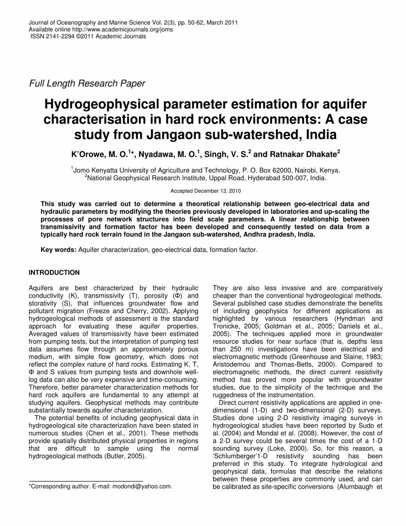
Regardless of the fact that, the geophysical data utilised for the case studies mentioned are basically the same, it has been recognised that there exists no universally accepted petrophysical models for converting geophysical data to hydro-geological attributes, partly due to, the scale and resolution disparity between hydrological and geophysical measurements (Ezzedine et al., 1999). In this study, establishing and verifying a field scale theoretical relationship between geo-electrical resistivity data and hydrogeological data has been carried out, in order to improve the characterization of aquifer parameters. The pore-scale geometrical relationships stipulated by Bernabe and Revil (1995) have been up-scaled to arrive at the field-scale relationship between transmissivity (T) and formation factor (Fa). The up-scaled model has been tested on data sets obtained from the Jangaon sub-watershed, Hyderabad, Andhra Pradesh, India. DESCRIPTION OF THE STUDY AREA The Jangaon sub-watershed, which falls under the greater Waipalli watershed, has an area of 28 km2 and is, situated about 80 km to the west of Hyderabad, Andhra Pradesh, India. It lies between longitudes 78.84°E and 79.92°E and latitudes 17.10°N and 17.14°N (Figure 1). Semi-arid climatic conditions prevail in the area, with minimum and maximum temperature of 22°C and 44°C, respectively. Drought conditions prevail for more than four months in any given year with April and May being the driest months. Geology Geology of the study area (Figure 2) consists of granites

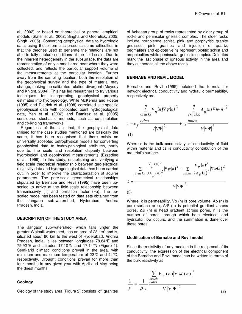
K’Orowe et al. 51 of Achaean group of rocks represented by older group of rocks and peninsular gneissic complex. The older rocks include hornblende schist, pink and porphyritic granite gneisses, pink granites and injection of quartz, pegmatites and epidote veins represent biotitic schist and amphibolites while peninsular gneissic complex. Dolerites mark the last phase of igneous activity in the area and they cut across all the above rocks. BERNABE AND REVIL MODEL Bernabe and Revil (1995) obtained the formula for network electrical conductivity and hydraulic permeability, respectively as:

( ) ( )

2

,

2)()(

2

2

Ψ∇

� ∇

+Ψ∇

∇�

=V

n

tubes

cracksnnpA

scV

nnn

tubes

cracks pV

fcc

ψψ

(1) Where c is the bulk conductivity, cf conductivity of fluid within material and cs is conductivity contribution of the material’s surface.

( )( )( )

( )

2

222

32

2)(3

3)(

Φ∇

∇�+∇�

=V

ntubes npA

npVn

cracks npA

npV

k

ϕϕ

(2) Where, k is permeability, Vp (n) is pore volume, Ap (n) is pore surface area, �� (n) is potential gradient across pores, �� (n) is head gradient across pores, n is the number of pores through which both electrical and hydraulic flow occurs, and the summation is done over these pores. Modification of Bernabe and Revil model Since the resistivity of any medium is the reciprocal of its conductivity, the expression of the electrical component of the Bernabe and Revil model can be written in terms of the bulk resistivity as:

2

2)()(

11

Ψ∇

∇

=

�

V

nnVn

tubescrack

p

f

ψ

ρρ (3)

52 J. Oceanogr. Mar. Sci.

Figure 1. Location of Jangaon Watershed in Nalgonda district, Andhra Pradesh, India.

Figure 2. Geological map of the Jangaon sub-watershed.

78.86 78.87 78.88 78.89 78.9 78.91

17.11

17.12

17.13

17.14

Longitude ( degrees)

Latitude ( degrees )

Andhra Pradesh

Jangaon Water shed

Map of India

Longitude L

atitude

78.86 78.87 78.88 78.89 78.9 78.91

17.11

17.12

17.13

17.14

M-1

M-2M-3M-4M-5

M-6

M-7

M-8M-9

M-10

M-11

M-12

M-13M-14

M-15M-16 M-17

Granite Gneiss Kankar Drainage Lineament

Longitude (degrees)

Latit

ude

(deg

rees

)

where, � is the bulk resistivity and �f is resistivity of water within the pores. Surface conduction is ignored since in hard rocks, fractures that act as the only conduction conduits. Even though tube-like pores contribute significantly to electric conduction, their contribution to hydraulic conduction is minimal in crystalline hard rocks. Equation 2 is therefore re-written as:

( )

2

22)]([3

3)]([

Φ∇

∇�

=V

ncracks npA

npV

k

ϕ

(4)

Let

( )V

nVP p

n =(specific pore volume),

( )V

npAns =

(specific pore surface)

( ) 2

2Ψ∇

∇=

npelectnw

ψ

and

( )2

2

Ψ∇

∇=

nphydrnw

ψ

The values wnelect and wnhydr determines the

weighted contribution of the pores in the electrical resistivity and hydraulic conductivity of the network and how well the pores are connected to the network. Then Equations 3 and 4 may, respectively, be re-written as:

�=

crackstubes

nPelectnw

fρρ11

(5)

�=cracks ns

nPhydrnwk 3

3

31

(6) Index ‘n’ refers only to pores where electrical and hydraulic conduction occurs. Equations 5 and 6 have one variable in common, namely, specific pore volume (Pn). This shows that the dependence of large-scale hydraulic and electrical properties on pore volume is as a con-sequence of the dependence of the network properties on the small-scale pore geometries. Wong et al. (1984) showed that networks possessing commonly observed skewed pore size distributions imply power law

K’Orowe et al. 53 relationships between small-scale electrical and hydraulic parameters and large scale pore volume and pore surface area. Because the Bernabe and Revil model can accommodate any pore size distribution including the bond shrinkage model of Wong et al. (1984), then the results of Wong et al. (1984), may be integrated into the hydraulic network and electrical equations of Bernabe and Revil (1995).

Whence k is directly proportional to 2S

km ��

�

����

�

φ where km

is defined as:

km = 12

1ln22

2

++

− xxx

> 0 (7)

and ρ

1

is directly proportional to

����

��

φφρ

m

f

1

, with φm being

expressed as:

φm=

01

ln2

2

>−xx

(8) Where x (0<x<1), is the factor by which the radius of the tube elements of Wong et al. (1984) model, are reduced. In modifying pore structure model of Bernabe and Revil to field scale model in the current study, transmissivity and apparent formation resisitivity factor (Fa) have been preferred, since they are both influenced by pore structure of a medium. Transmissivity is also related to hydraulic conductivity, which, in turn is a constant of proportionality that relates water flux (specific discharge, q) and the hydraulic head gradient (h) in Darcy’s law. It is directly proportional to the intrinsic permeability (k), reflecting the geometry of the pore system and the properties of the flowing fluid as:

hKqJ hydr ∇−== (9)

���

����

�=µδg

kK (10)

Where � is the fluid density, � is its dynamic viscosity and g is the acceleration due to gravity. The transmissivity (T), of an individual fracture of aperture (ac) can be expressed in terms of the hydraulic conductivity (K) as:

54 J. Oceanogr. Mar. Sci.

µδg

kaKaT cc == (11)

Therefore, the water flux may be written as:

haT

qjc

hydr ∇−== (12)

The electrical flow in a medium on the other hand is similarly expressed in terms of current flux and potential gradient as:

VAi

jelect ∇==ρ1

(13) The electrical property, the apparent formation resistivity factor (Fa) is expressed as:

faF

ρ

ρ= (14)

Electric flux is therefore expressed in terms of apparent formation resistivity factor as:

VFA

ij

fa

elect ∇==ρ1

(15) For this reason, apparent formation factor and transmissivity will determine the aquifer’s electrical and hydraulic properties, respectively. The use of apparent formation factor eliminates the effect of changes in water resistivity but utilizes the information on these changes. Since the matrix is non-conductive, the transmissivity of any interval of aquifer is calculated by summing the transmissivity of the fractures within that interval. Where an interval contains a single fracture, then transmissivity is simply equal to the transmissivity of that fracture. From the power laws of Wong et al. (1984), proportionality relations between bulk resistivity and intrinsic permeability with the porosity fraction, on introducing proportionality constants, A and B, respectively, can be expressed as:

A=ρ

1����

��

φφρ

m

f

1

(16)

K = B2

)(

S

mkφ

(17)

To make k the subject, Equation 17 is divided by Equation 16 to obtain.

12 −−− ��

���

����

����

�

= ρφρφ φmk

m

fSkA

B

(18) Writing K in terms of k from Equation 10, the hydraulic conductivity is expressed as:

12 −−− ��

���

����

����

�

= ρφρφµ

δ φmk

m

fSg

KA

B

(19) From Equation 11, transmissivity may be written as:

12 −−− ��

�

����

�

= ρρφµδ φ

fSg

aTm

km

cA

B

(20)

Where φφ m

aF1−= is Archie’s law (Archie, 1942)

But, � = faF ρ.

Substituting these values into Equation 20, we obtain

112 −−−����

�

�

����

�

�

−= ff aamk

m

ac FSFFg

aTA

B ρρµδ

φ (21)

Taking the natural logarithms of both sides of Equation 21, we get

( ) ac F

mm

Sga

T k

A

Blnlnln 2

φµδ

−���

����

�= −

(22) Equation 22 is therefore, the modified Bernabe and Revil relationships, which in this case relates the field parameters, transmissivity and apparent formation factor. The equation is a general form of a linear graph of the form Y = a+bX (23) Where

X = ln Fa, Y = ln (T), a =���

����

� −2ln Sga

A

B c

µδ

, and b = - φm

mk

The terms a and b are the correlation coefficients

K’Orowe et al. 55

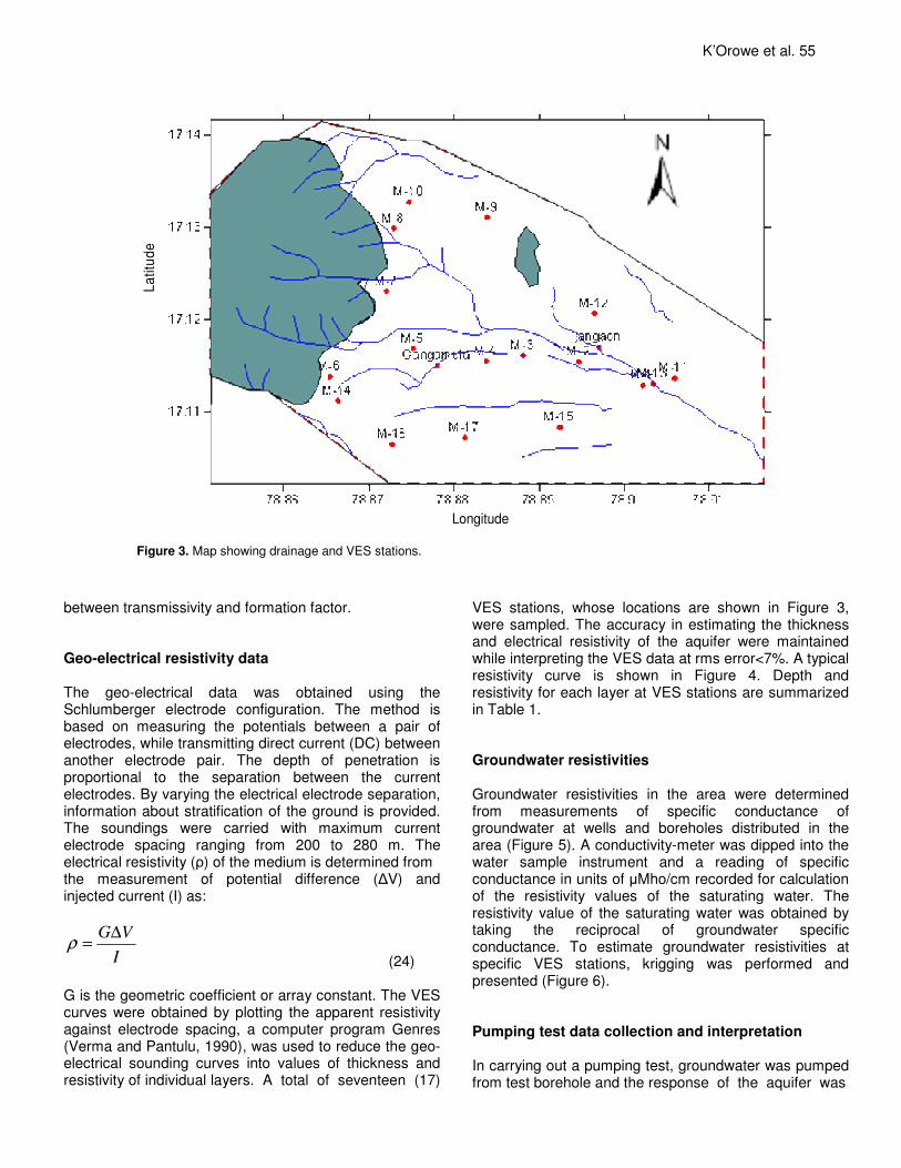
Figure 3. Map showing drainage and VES stations.

between transmissivity and formation factor. Geo-electrical resistivity data The geo-electrical data was obtained using the Schlumberger electrode configuration. The method is based on measuring the potentials between a pair of electrodes, while transmitting direct current (DC) between another electrode pair. The depth of penetration is proportional to the separation between the current electrodes. By varying the electrical electrode separation, information about stratification of the ground is provided. The soundings were carried with maximum current electrode spacing ranging from 200 to 280 m. The electrical resistivity (�) of the medium is determined from the measurement of potential difference (�V) and injected current (I) as:

IVG∆=ρ

(24) G is the geometric coefficient or array constant. The VES curves were obtained by plotting the apparent resistivity against electrode spacing, a computer program Genres (Verma and Pantulu, 1990), was used to reduce the geo-electrical sounding curves into values of thickness and resistivity of individual layers. A total of seventeen (17)

VES stations, whose locations are shown in Figure 3, were sampled. The accuracy in estimating the thickness and electrical resistivity of the aquifer were maintained while interpreting the VES data at rms error<7%. A typical resistivity curve is shown in Figure 4. Depth and resistivity for each layer at VES stations are summarized in Table 1. Groundwater resistivities Groundwater resistivities in the area were determined from measurements of specific conductance of groundwater at wells and boreholes distributed in the area (Figure 5). A conductivity-meter was dipped into the water sample instrument and a reading of specific conductance in units of �Mho/cm recorded for calculation of the resistivity values of the saturating water. The resistivity value of the saturating water was obtained by taking the reciprocal of groundwater specific conductance. To estimate groundwater resistivities at specific VES stations, krigging was performed and presented (Figure 6). Pumping test data collection and interpretation In carrying out a pumping test, groundwater was pumped from test borehole and the response of the aquifer was

Latit

ude

Longitude

56 J. Oceanogr. Mar. Sci.

Figure 4. Typical geo-electrical curves for the study area.

Figure 5. Specific conductance values (µmhos cm-1) at various points within Jangaon.

measured in the same or nearby observation boreholes. A model was then used to estimate transmissivity values from the aquifer response. Three single well test and two tests using observation wells were conducted. The heterogeneity of the hard rock system has been modelled as an equivalent porous medium. Thus, the primary and

secondary porosity and the transmissivity distribution are replaced with a continuous porous medium having equivalent hydraulic properties. The Jacob’s method has been used in conjunction with the Neumann et al. (1984) method for interpretation of the pumping tests. Pumping tests were done on the boreholes in locations W-1, W-2,

Longitude (degrees)

Latit

ude

(deg

rees

)

78.88

K’Orowe et al. 57

Figure 6. Distribution of kriged specific conductance (�mhos cm-1).

Figure 7. Location of pumping test boreholes, Jangaon sub-watershed

W-3, W-4, and W-5 (Figure 7). Aquifer bulk resistivities at pumping sites have been obtained from krigged estimates of aquifer resistivity data from VES stations (Figure 8). Aquifer layers have been taken as those overlying the basement layer. The tests consisted of two phases: the productive phase which lasted 1 h followed by a recovery phase, which was maintained until the

water level in the borehole recovered or until three readings in succession were identical. During the aquifer test, records of water levels before and after pumping, well discharge rate and the duration of the pumping test were made. The measurement of water levels was carried out in the pumped wells using an electric sounder, which is triggered when the tape is in contact with water

Longitude (degrees)

La

titud

e (d

egre

es)

58 J. Oceanogr. Mar. Sci.

Figure 8. The distribution of the resistivity of the saturated aquifer. (Note; VES stations are marked M-1, M-2, M-3………….e.t.c, Pump test boreholes are marked W-1, W-2, W-3, W-4 and W-5).

surface. After pumping is stopped, water levels were allowed to rise. For 100% recovery, static water levels before pumping and the water levels at the end of the pumping test will be equal.

The hydrogeological characteristics of the aquifer in the Jangaon are that groundwater is primarily associated with fractures zones. A common feature in these types of aquifers is that locally, the aquifer acts as a confined reservoir whereas regionally, it is unconfined, since fractures are commonly in contact with suspended groundwater near the surface or with standing surface water in depressions. For this reason, the analysis has been undertaken using the Cooper and Jacob (1946) straight-line method, where drawdown is plotted with an arithmetic scale on the y-axis against logarithmic time scale on the x-axis. Transmissivity is then estimated from the pumping rate, and change in drawdown per log-cycle. The procedure is included in the Groundwater for windows (GWW) software (Braticevic and Karanjac, 2000) used in our interpretation. Transmissivity results obtained from pumping test have been appropriately adjusted using the Neumann et al. (1984) method, to take into consideration the anisotropic nature of hard rock environments. Typical pumping curves are shown in Figure 9. DATA ANALYSIS, RESULTS AND DISCUSSION The modified Bernabe and Revil theoretical model

(Equation 22) was calibrated using field observations in the Jangaon sub-watershed. Parameters used in the calibration of the Bernabe and Revil model are shown in Table 1, while Figure 11 is a plot of logarithm of formation factor from electrical soundings versus logarithm of transmissivity from pumping tests. The resultant curve shows a negative slope in agreement with theoretical calculations given by Equation 22. The observed relationship is expressed by Equation 29, with correlation coefficient of 90%, showing that apparent resistivity factor is correlated well with transmissivity. From Figure 10, the relationship between transmissivity and apparent formation factor is given by: ln (T (m2/day)) =-2.5ln Fa +9.9 (25) Equation 25 is the calibration model of the Jangaon sub-watershed. So as to have dimensional coherence, the gradient and intercept of the curve are in units of m2/day, while apparent formation factor has no units, it being a quotient of resistivity values. By incorporating the modified Bernabe and Revil model into the calibration model of the Jangaon sub-watershed, the gradient is expressed in terms of bond shrinkage factor, x, as:

5.2ln

11

21

ln22

2

2

2

=�

��

−�

��

++

−==

xx

xxx

m

mb k

φ (26)

Longitude (degrees)

La

titud

e (d

egre

es)

K’Orowe et al. 59

Figure 9. Pumping test curve for borehole W-1 after adjustment for anisotropy.

Equation 26 can be re-written as

( )5.2

ln12

2 2 =�

��

−+=x

xm

mk

φ (27) Equation 27 reduces further to

xx ln22 =− (28)

Equation 28 can be broken into two equations given by

22 −= xy and xy ln= (29) When Equations 28 and 29 are plotted on the same graph for values of 0<x<1, the point of intersection of the two functions shown in Figure 11, is the solution required. Figure 11 shows that, the two curves intersect at a point where the value of 10x is 2, for values of 0<x<1. This gives the value of x as 0.2, therefore the cementation

60 J. Oceanogr. Mar. Sci.

Table 1. Electrical and hydraulic parameters at the pumping test boreholes.

Borehole T (m2/day) � (Ohm-m) EC (�Mho/cm) �f (Ohm-m) Fa W-1 44.2 112.2 992 10.08 11.13 W-2 24.7 156.5 895 11.17 14.01 W-3 45.7 133.1 853 11.72 11.36 W-4 37.6 112.2 1033 9.68 11.59 W-5 35.1 150.2 835 11.97 12.55

Figure 10. Transmissivity formation factor relationships.

Figure 11. Successive approximations of the functions 2x-1 and lnx for values 0<x<1

factor ���

����

�

−=

1ln

2

2

xx

mφ

will be (4.3=φm

). The negative correlation is consistent with the interpretation of electrical flow through pore volumes rather than through surface clay conduction. The trend and nature of the

apparent formation factor-transmissivity relationship for the aquifer in the Jangaon sub-watershed has therefore been established. With the development of generalized relationship (Equation 25), it is now possible to characterize transmissivity using geo-electric models within the Jangaon sub-watershed.

Hydraulic conductivity values were obtained from transmissivity values, using Equation 11, where the pore scale fracture aperture (ac) is replaced by a field scale aquifer thickness (be). Hydraulic conductivity values at each VES station are shown in Table 2. It should be noted that only VES stations with aquifer resistivities of more than 50 Ohms have been considered, according to the aquifer ranges of Gangadhara (1992). The distri-bution of the same data using ordinary kriging is shown in Figure 8. CONCLUSION From the theoretical work of Bernabe and Revil, (1995) and the bond shrinkage model of Wong et al. (1984), the

lnT = -2.5lnFa + 9.9R2 = 0.9

3.1

3.2

3.3

3.4

3.5

3.6

3.7

3.8

3.9

2.4 2.45 2.5 2.55 2.6 2.65 2.7

Log

tran

smis

sivi

ty (

ln T

)

Log formation factor (ln Fa)

-2.5

-2

-1.5

-1

-0.5

0

1 2 3 4 5 6 7 8 9

2x-2

, ln

x

10x

2x-2

lnx

K’Orowe et al. 61

Table 2. Summary of parameters at VES stations.

Station ρ (Ohm-m) eb(m) EC (�Mho/cm) ECf

10000=ρ

(Ohm-m) T (m2/day) K (m/day)

M-1 178.23 13.46 1125 8.89 20.05 11.07 0.822 M-2 163.09 26.03 999 10.01 16.29 18.61 0.715 M-3 82.94 15.55 1265 7.91 10.49 55.92 3.596 M-4 209.15 9.99 1049 9.53 21.95 8.83 0.884 M-5 187.86 10.64 846 11.82 15.89 19.80 1.861 M-7 91.41 19.47 690 14.50 6.30 200.06 10.275 M-8 212.25 9.37 694 14.45 14.69 24.10 2.572 M-9 82.71 22.82 823 12.15 6.81 164.68 7.216

M-11 170.10 8.8 1034 9.67 17.59 15.36 1.745 M-12 196.08 6.15 828 12.08 16.23 18.78 3.034 M-13 240.47 4.04 1083 9.23 26.05 5.75 1.423 M-16 163.6 24.84 591 16.92 9.67 68.54 2.759 M-17 95.83 10.8 900 11.10 8.63 86.76 8.033

pore-scale network equations have been modified to develop a field scale theoretical relationship between, transmissivity (T) and apparent formation resistivity factor (Fa). A negative linear relationship between natural logarithm of transmissivity and apparent formation factor

(that is,

( ) ac F

mm

Sga

T k

A

Blnlnln 2

φµδ −��

�

����

�= −

) has been noticed. The intercept in the equation is solely dependent on the specific surface area, for a given fracture aperture. The gradient on the other hand is dependent on the bond shrinkage factor (<0x<1) of Wong et al. (1984) which determines size of pore volumes.

The negative linear relationship means that as trans-missivity increases, apparent formation factor decreases. This is consistent with a mode of flow influenced by flow through pore volume. Applying the modified Bernabe and Revil relationship, on data acquired at the Jangaon sub-watershed has also produced a negative linear relationship (that is, ln (T (m2/day)) = -2.5ln Fa +9.9) replicating the relationship predicted by theory. A value of 3.4 has, therefore, been determined as the cementation factor for the geological material of the aquifer of the area. One cannot, however, expect that the apparent formation factor and transmissivity dependence found for the Jangaon sub-watershed to be invariably applicable to any hard rock environment. However, a cost effective and non-invasive quantification of transmissivity from geo-electrical methods is obtained. REFERENCES Alumbaugh DL, Chang PY, Paprocki L, Brainard JR, Glass RJ,

Rautman CA (2002). ‘Estimating moisture contents in the vadose zone using cross-borehole ground penetrating radar: A study of accuracy and repeatability’ Water Resour. Res., 38: 1309.

Aristodemou E, Thomas-Betts A (2000). ‘D.C resistivity and induced polarization investigations at a waste disposal site and its environments’, J. Appl. Geophys., 44: 275-302.

Bernabe Y, Revil A (1995). ‘Pore-scale heterogeneity, energy dissipation and the transport properties of rocks’, Geophys. Res. Lett., 22(12): 1529-1532.

Braticevic, Karanjac (2000). ‘Groundwater software manual’, United Nations, New York

Butler JJ Jr (2005). ‘Hydrogeological methods for estimation of spatial variations in hydraulic conductivity’, Hydrogeophysics, edited by Y. Rubin and S.S. Hubbard, Springer, Netherlands, Central groundwater board of India, 2003, ‘Occurrence, Genesis and Control Strategies of Fluoride, Waipalli Watershed, Nalgonda District Andhra-Pradesh, India’, Central Groundwater Board, Ministry of Water resources, Government of India, pp. 23-58.

Chen J, Hubbard S, Rubin Y (2001). ‘Estimating the hydraulic conductivity at the South Oyster Site from geophysical tomographic data using Bayesian techniques based on the normal linear regression model’, Water Resources Res., 37(6): 1603-1613.

Cooper HH, Jacob CE (1946). ‘A generalized graphical method for evaluating formation constants and summarizing well field history’, Transaction American Geophysical Union 27: 526-534.

Daniels JJ, Allred B, Binley A, Debrecque, Alumbaugh D (2005). ‘Hydrogeophysical case studies in the Vadose zone’, In Hydrogeophysics, edited by Rubbin, Y and Hubbard, SS., Springer, Netherlands. pp. 413-440.

Dietrich PT, Whittaker, Teutsch G (1998) ‘An integrated hydrogeophysical approach to subsurface characterization’, GQ 98

Conference, Tubngen, Federal Republic of Germany, and (Luvain): International Association of Hydrological Sciences. pp. 513-519.

Ezzedine S, Rubin Y, Chen J (1999) ‘Bayesian method for hydrogeological site characterization using borehole and geophysical survey data: theory and application to the Lawrence Livermore National Laboratory Superfund site’, Water Resources Res., 35(9): 2671-2683.

Freeze RA, Cherry JA (1979). ‘Groundwater’, prentice hall Inc. Englewood Cliffs, New Jersey.p.7

Gangadhara TR (1992). ‘Groundwater exploration techniques’, Lecture notes, National Geophysical Research Institute.

Goldman M, Gvirtzman H, Meju MA, Shtivelman V (2005). ‘Case studies at the regional scale’, In Hydrogeophysics, edited by Rubbin, Y and Hubbard, S.S, Springer, Netherlands. pp. 361-390

Greenhouse JP, Slaine DD (1983). ‘The use of reconnaissance electromagnetic methods to map contaminant migration’,

Groundwater Monitor Rev., 3(2): 47-59.

faF

ρρ=

62 J. Oceanogr. Mar. Sci. Hyndman D, Tronicke J (2005). ‘Hydrogeophysical case studies at the

local scale: The saturated zone’, In Hydrogeophysics, edited by Rubbin, Y and Hubbard, SS., Springer, Netherlands, pp. 391-415

Loke MH (2000). ‘Electrical Imaging Surveys for environmental and engineering studies: A practical guide to 2D and 3D surveys’, University of Birmingham.

McKenna SA, Poeter EP (1995). ‘Field example of data fusion in site characterization’, Water Resour. Res., 31(12): 3229-3240.

Mondal NC, Rao VA, Singh VS, Sarwade DV (2008). ‘Delineation of concealed lineaments using electrical resistivity imaging in granitic terrain’, Curr. Sci.. 94(8): 1023-1030.

Moysey S, Knight RJ (2004). ‘Modeling the field-scale relationship between dielectric constant and water content in heterogeneous systems’, Water Resource’, 40(3): 3510.

Neumann SP, Walter, GP, Bently HW, Ward JJ, Gonzales DD (1984). ‘Determination of horizontal anisotropy with three wells’, Groundwater, 22(1): 66-72.

. Ramirez AL, Nation JJ, Hanley WG, Aines R, Glacer RE, Sengupta SK, Dyer KM, Hickling TL, Daily WD ( 2005). ‘Stochastic inversion of electrical resistivity changes using a Markov Chain Monte Carlo Approach’. J. Geophysical Res., 110:BO2101, DOI: 10:1029/2004JBOO3449.

Singh KP (2005). ‘Nonlinear estimation of aquifer parameters from surficial resistivity measurements’, J. Hydrol. Earth Sci., 2: 917-938.

Singha K, Gorelick SM (2005). ‘Saline tracer visualized with electrical

resistivity tomography: field scale moment analyses, Water Resources Res., 41, WO5023, doi: 10.1029/2004WR003460.

Sudo H, Tanaka T, Kobyashi T, Miyamoto M, Amagai M (2004). ‘Permeability imaging in granitic host rocks based on surface resistivity profiling’, J. Exploration Geophys., 57(1): 56-61.

Slater L, Binley A, Versteg R, Cassiani G, Birken R, Sandberg S (2002). ‘A 3D ERT study of solute transport in a large experimental tank’, J. Appl. Geophys., 49: 211-229.

Verma SK, Pantulu KP (1990). ‘Software for the interpretation of resistivity sounding data for groundwater exploration’ National Geophysical Research Institute, Hyderabad-INDIA.

Wong P, Koplick J, Tomanic JP (1984). ‘Conductivity and permeability of rocks’, Phys. Rev. Bull., 30: 6606-6614.

Yeh TC, Liu S, Glass J, Baker K, Brainard JR, Alumbaugh DL, Labreque D (2002). ‘A geostatistical based inverse model for electrical resistivity surveys and its application to vadose zone hydrology’, Water Resour. Res., 39(3): 13-14.