characterisation of the components in cataclysmic variablesclok.uclan.ac.uk/7961/1/gabriel william...
TRANSCRIPT

Characterisation of the Components in Cataclysmic Variables
Gabriel William Pratt
A thesis submitted in partial fulfilment
of the requirements for the degree of
Doctor of Philosophy.
Centre for Astrophysics
Department of Physics, Astronomy and Mathematics
University of Central Lancashire
December 1999

Declaration
The work presented in this thesis was carried out in the Department of Physics, Astronomy
and Mathematics, University of Central Lancashire. Unless otherwise stated it is the
original work of the author.
While registered for the degree of Doctor of Philosophy, the author has not been a regis-
tered candidate for another award of the University. This thesis has not been submitted
in whole, or in part, for any other degree.
Gabriel William Pratt
December 1999

Abstract
This thesis presents new and archive X-ray, optical and ultraviolet observations of
cataclysmic variables, and discusses the results obtained in the context of the relationship
between the physical and spectral components visible. It concentrates on the eclipsing
dwarf nova OY Carinae, which has been observed both in superoutburst and quiescence.
Optical 'wide B' band light curves were obtained at the end of the 1994 superoutburst
and on the decline. Eclipse mapping of these light curves reveals an accretion disc with a
considerable physical flare (rs 100). These are the first maps of a disc in the superoutburst
state that clearly show such flaring. Contemporaneous X-ray observations were obtained
with the ROSAT HRI. No eclipse of the X-ray flux was detected, a similar result to
that obtained from the EXOSAT observations of the 1985 superoutburst by Naylor et al.
(1988), supporting the case for the existence of a coronal component source for the X-rays
in high accretion rate systems.
Later ROSAT observations of OY Car in quiescence are presented. A 1994 PSPC
observation allows constraints to be placed on the quiescent X-ray spectrum. OY Car
returns similar values for the temperature of the emitting gas and the emission measure
as its fellow eclipsing systems. It is difficult, however, to reconcile the column density
inferred from the X-ray observation with that found from HST ultraviolet observations.
A column density of nH 1022 cm 2 , found in the 'iron curtain' study by Home et al.
(1994), is not compatible with the X-ray spectrum.
New optical photometry, obtained during quiescence in 1998, is used to update the
orbital ephemeris of the system. A further ROSAT HRI light curve, obtained in quiescence
with good phase coverage, is presented. It displays an eclipse of the X-ray flux, detected
at the 13a level, which is coincident with the optical eclipse of the primary and suggests
that the region of X-ray emission is comparable in size to the white dwarf. This confirms
that the boundary layer region is visible in OY Car in quiescence, and, in common with
similar systems, implies that the boundary layer is the source of the X-ray flux during
periods of low mass accretion. The general picture of the X-ray emission from CVs, which
has been built up from observations of different objects using different satellites, has thus
been confirmed for the first time for the same object using the same satellite.
The fact that the quiescent boundary layer can be seen, and that the soft X-ray flux is
not extinguished, together suggest that the 'iron curtain' may be variable and connected
to the accretion. The thesis also explores for the first time the effect a 'warm absorber'

would have on the X-ray spectrum and the deduced column densities of high inclination
CVs in quiescence.
The application of synthetic spectral analyses to ultraviolet observations of CVs is ex-
tensively reviewed, with particular emphasis on the spectral components observed. White
dwarf model atmospheres and synthetic spectra are generated using TLJUSTY and SYN-
SPEC, and those JUE spectra of cataclysmic variables where the white dwarf can be seen
are modelled using a x2 fitting routine. White dwarf synthetic spectra veiled by an 'iron
curtain' are also calculated and applied to JUE archive observations of OY Car and similar
systems. The resulting independently estimated white dwarf temperatures are compared
with published values and with temperatures obtained from the application of different
model atmosphere codes. The column density found by Home et al. (1994) is confirmed.
JUE archive observations of U Gem show a similar cooling time ('-.' 30 days) to more recent
HST observations. It is shown that the major source of systematic error in estimating the
white dwarf temperature from ultraviolet observations is uncertainty in the masses of the
white dwarfs.
The final Chapter shows how scheduled (simultaneous) HST and ASCA observations
of OY Car in quiescence will be used to place further constraints on the temperature of the
emitting gas and the column density, and how the techniques developed for the ultraviolet
modelling can be applied to the HST data. Future (accepted) XMM observations of
UX UMa, to constrain spectral components in the high mass accretion rate regime, are
also discussed.

Contents
1 Introduction 1
1.1 The Cataclysmic Variable Zoo ..........................2
1.2 Accretion discs: energy considerations and X-ray production ........4
1.3 Accretion discs: behaviour models .......................10
1.4 The 'iron curtain' .................................17
1.5 Thesis Overview .................................19
2 Optical observations of the 1994 Feb superoutburst of OY Carinae 21
2.1 Introduction .................................... 21
2.2 Observations and data reduction ........................ 22
2.2.1 The light curves ............................. 22
2.3 Mapping the disc ................................. 26
2.3.1 Review of the eclipse mapping method ................. 26
2.3.2 Mapping the 1994 Feb superoutburst disc ............... 33
2.4 Discussion - flare angles and temperature distributions ............ 39
2.5 Conclusions .................................... 42
3 ROSAT X-ray observations of the 1994 Feb superoutburst of OY Carinae 44
3.1 Introduction .................................... 44
3.2 The ROSAT Satellite . . . . . . . . . . . . . . . . . . . . . . . . . . . . . . 47
3.3 Observations and data reduction ........................ 49
3.4 The Superoutburst X-ray light curve ...................... 51
3.5 The Superoutburst Luminosity ......................... 51
3.6 Discussion ..................................... 54
3.6.1 Comparison with VW Hyi ........................ 54
3.7 Conclusions .................................... 60
II

4 Optical and X-ray observations of OY Carinae in quiescence 63
4.1 Introduction .................................... 63
4.2 Observations and data reduction ........................ 66
4.2.1 PSPC X-ray and WFC EUV observations, 1994 July ......... 66
4.2.2 Optical observations and HRI X-ray observations, 1998 Jan - Mar . 67
4.3 The orbital ephemeris .............................. 70
4.3.1 Optical eclipse timing measurements .................. 70
4.3.2 Method .................................. 74
4.4 The X-ray data .................................. 76
4.4.1 Spectral analysis of the 1994 July ROSAT PSPC observation . . . . 76
4.4.2 The 1998 Jan ROSAT HRI observation - an X-ray eclipse ...... 81
4.5 Discussion ..................................... 84
4.5.1 The quiescent X-ray spectrum ..................... 84
4.5.2 The quiescent luminosity, the eclipse and the absorption ....... 85
4.6 Conclusions .................................... 89
5 Modelling of ultraviolet data in quiescence: critical review 91
5.1 Overview ..................................... 91
5.2 lUll: the satellite and data archive ........................ 92
5.3 Non-magnetic CVs in the ultraviolet ...................... 96
5.3.1 Observational characteristics ...................... 96
5.3.2 Boundary layer temperatures from ultraviolet observations of CV
winds................................... 99
5.4 The white dwarf primary ............................ 102
5.4.1 Detection ................................. 103
5.4.2 Temperature determination of the primary .............. 104
5.4.3 Other measurable primary parameters ................. 108
5.4.4 Summary ................................. 110
5.5 Spectrum dearchival and initial development of the fitting process ..... 110
5.6 Model construction using TLUSTY and SYNSPEC .............. 119
5.6.1 The basics of TLUSTY ......................... 121
5.6.2 Calculating the model atmospheres and synthetic spectra ...... 123
5.7 Spectral Modelling ................................ 128
5.7.1 Overview and some caveats ..................... 128
5.7.2 Some synthetic spectral analyses .................... 129
III

5.8 Discussion . 143
5.9 Summary and conclusions ............................149
6 Conclusions and Further work 151
6.1 Summary of results and conclusions ......................151
6.2 Further work ...................................154
6.2.1 Forthcoming observations with ASCA and the HST ......... 154
6.2.2 Future observations ...........................159
Appendices 164
A The Zanstra method applied to CV winds
164
B Overview of the basic equations used in model stellar atmosphere gen-
eration 166
C Details of TLUSTY and SYNSPEC input and output files 171
D Acronyms used 175
References 177
iv

Acknowledgements
I offer great thanks and appreciation to my supervisor, Barbara Hassall, for her support and encouragement, instruction, guidance and useful advice. And for her patience when faced with multiple drafts of this work. Thanks are also extended to Gordon Bromage, for his invaluable assistance and encouragement in his role as second supervisor.
Thanks to Tim Naylor, Janet Wood and Koji Mukai, with whom I have had many fruitful collaborations and stimulating discussions during days at Keele and elsewhere. Constance Ia Dous extended outstanding hospitality and provided valuable insights into ultraviolet observations during a visit to Sonneberg Observatory. Very helpful conversa-tions pertaining to the work in this thesis were had with Ed Sion while in Sonneberg and with the staff at the University Observatory, Gottingen: Klaus Beuermann, Rick Hessman, Boris Gänsicke and Klaus Reinsch. Martin Barstow kindly got me started on TLUSTY and SYNSPEC, and Ivan Hubeny provided essential files and very useful recommendations for using his programs. I am grateful to the staff at SAAO, particularly Fred Marang and Dave Buckley, for help with the telescope and the data reduction, respectively. I thank the ROSAT scheduler, Jakob Engelhauser, for flexibility as to the choice of time slots I wanted in 1998 Jan-Feb. My thanks to the observers of the Variable Star Section of the Royal Astronomical Society of New Zealand, and especially Frank Bateson, who supplied the data on OY Car. Matt Burleigh helped with the access to my data from the 1998 ROSAT run. I thank Andy Adamson and Pete Newman for providing essential computing support as STARLINK Managers. I acknowledge the use of facilities provided by the PPARC STARLINK project, and I acknowledge the financial support of a research studentship from the University of Central Lancashire.
I am very grateful to my friends and colleagues at the University of Central Lancashire and elsewhere, who have helped no end in making the last few years more bearable with the benefit of shared experience. It is a long list, but you know who you are. Many thanks, too, to my friends in Ireland, who have supported me and kept in contact through all this and over the years since we all left (and in some cases didn't leave, or left and returned to) Ballyhaunis.
Finally, I wish to give special thanks to my parents and family for all they have done for me, for their faith in me, for their support and for their encouragement. It is something of a cliché to refer to formative experiences in acknowledgements such as this, but I feel I must point out that the night sky in the West of Ireland can be breathtaking. I am forever grateful to my parents for bringing me up in such a way as to enable me to appreciate this fact.
This thesis is dedicated to the memory of my brother, Adam, and to the memory of my dear friend, Anne Marie O'Loughlin.

Chapter 1
Introduction
This thesis is concerned with observations of dwarf novae, a subclass of non-magnetic
cataclysmic variable binary star, and in particular with one example, OY Carinae. Mu!-
tiwavelength data are used to probe various aspects of this intriguing system in both the
superoutburst and quiescent states. Further simultaneous time on the Hubble Space Tele-
scope (HST) and the Advanced Satellite for Cosmology and Astrophysics (ASCA) has been
awarded, and is scheduled for 2000 Mar, giving coverage of the system in high resolution
X-ray and ultraviolet wavelengths. In this connection, a critical review of the modelling
techniques for ultraviolet spectra has been undertaken and is also presented. The review
utilises archive data of many cataclysmic variable systems from the now defunct Interna-
tional Ultraviolet Explorer (IUE) satellite and from the HST archive itself.
OY Car is a well studied system because of two attributes in particular: its inclination
and its short orbital period. It is a deeply eclipsing cataclysmic variable, with an inclination
of i = 83°, a value which allows the identification of the physical components of the system
through timing observations throughout its 91 min orbit. As such it is a member
of a relatively select group of cataclysmic variables. Moreover, the quality of modern
spectroscopic observations, across wavelengths ranging from infrared to X-ray, has allowed
the identification of spectral components which can be directly related to the energy
process taking place, and so to the physical components themselves. While theory has been
successful in explaining much of the observed behaviour, there are still many interesting
problems which can be addressed with further observations. Interpretation of data from
eclipsing systems like OY Car offers a further challenge chiefly because of inclination
effects.
The optical, X-ray and ultraviolet observations presented here address some of the
outstanding problems, such as the effect of the 'iron curtain' seen in high inclination sys-
1

tems. The results are discussed in the context of similar observations of lower inclination,
non-eclipsing systems.
The remainder of this Chapter describes the different types of cataclysmic variable,
their respective physical components, and how the physical processes give rise to the emis-
sions studied in this thesis. Note that, in keeping with the conventions of the cataclysmic
variable community, cgs or solar units are used throughout.
1.1 The Cataclysmic Variable Zoo
Up to 70% of all stars may be members of binary or multiple systems. This thesis deals
with the cataclysmic variables (CVs), which are close binary stars consisting of a white
dwarf (the primary) accreting matter from a late-type, quasi-main sequence star (the
secondary). CVs are, as a class, characterised by variations in all wavelengths on a wide
variety of timescales, all connected to the accretion process. In many cases this accretion
is in bursts, resulting in large releases of energy, hence 'cataclysmic'. Within the standard
white dwarf/main sequence star paradigm, however, a very wide variety of behaviour is
displayed. The classification scheme has subclasses and subclasses of subclasses'.
The most basic classification scheme is drawn from the way in which matter is accreted
from the secondary star onto the white dwarf. While magnetic fields undoubtedly play a
large role in all CVs, the magnetic field of the primary can control the accretion flow only
if the field strength is > 10 5 C.
CVs with a relatively weak magnetic field (< 10 C) are characterised by the fact
that the transferred material forms an accretion disc around the primary star. Such non-
magnetic CVs (a relative term) are the subject of this thesis, and all have this binary
and accretion disc structure. The physical purpose of the disc is to enable the transfer of
mass inwards, to be accreted onto the white dwarf, and the transfer of angular momentum
outwards. The point of impact of the mass transfer stream from the secondary star with
the edge of the accretion disc is called the bright spot.
The physical components of a typical nonmagnetic CV, and their characteristic energy
ranges are: the secondary (infrared - optical), the white dwarf (optical - ultraviolet), the
accretion disc (infrared - extreme ultraviolet [EUV]), the bright spot (optical - ultraviolet)
and the boundary layer between the accretion disc and the surface of the white dwarf
(EUV - X-ray).
'Once memorably described as "over Balkanisation" by Patterson et al. (1997b; as they defined yet
another subclass).
2

The non-magnetic CVs are subclassified into several categories according to their re-
spective long-term photometric behaviour, which is directly a result of the mode of accre-
tion onto the white dwarf. These categories are (organised after Warner's comprehensive
review 1995):
• Classical novae, which have had only one observed eruption. The range from pre-
nova brightness to maximum is from 6 to 19 magnitudes. The largest amplitude
eruptions with shortest duration are in the very fast novae (days); the lowest ampli-
tude, are in the slow novae, with durations that may last for years. The mechanism
for the eruptions is thermonuclear runaway of the accreted material on the surface
of the white dwarf.
• Recurrent novae are previously recognised novae that have repeated. The main
spectroscopic distinction between these types and the following dwarf novae is that
classical and recurrent novae are observed to eject a substantial shell of material.
• Dwarf novae, which are subject to smaller amplitude quasi-periodic outbursts ("
3 - 5 magnitudes) on timescales ranging from tens of days to tens of years. The
outbursts are due to a release of gravitational energy after a sudden increase in the
rate of mass transfer through the accretion disc. Dwarf novae are further subclassified
after their respective prototypes as follows:
Z Cain stars show standstills 0.7 magnitudes below maximum, during which
outbursts proper can cease for tens of days to years;
SU UMa stars are subject to occasional superoutbursts (on timescales of hundreds
of days) in addition to normal dwarf nova outbursts, rising to r,s 0.7 magnitudes
above normal outburst maximum and lasting ".s 5 times as long. There is a
further subclass of extreme SU UMas, designated ER UMa stars, which have
unusually high mass transfer rates and show extremely short intervals between
superoutbursts (19- 44 d) and a very short normal outburst interval (3- 4 d);
U Gem stars include all other dwarf novae.
• Novalike variables, which are thought to be pre-novae, post novae, and Z Cam
stars that are in permanent standstill. They are observed as such because the ob-
servational baseline available to us (rJ 100 years) is too short to reveal a change in
their state. This class includes the VY Scl stars, which are observed to undergo
occasional reductions from approximately constant magnitude, thought to be due to
a temporary reduction of the mass transfer rate.
3

In those CVs where the primary has a large magnetic field (> io C), the gas stream
material retains its identity only until the magnetic field of the primary is able to control
the flow. At this point the stream material locks onto the magnetic field lines and is
accreted along them, to impact onto the surface of the primary in an accretion column.
In those systems where the magnetic field strength of the primary is sufficient to cause
synchronisation of the rotation period of the white dwarf and the orbital period, accretion
is along the field lines and the system is a polar or AM Her star. With less powerful
magnetic fields, synchronism cannot be achieved. If the magnetic moment of the white
dwarf is small, an accretion disc can form but this is truncated at the inner edge, and
subsequent accretion is along field lines. These are the intermediate polars, which, as
a class, display a wide variety of periodic phenomena.
But non-magnetic CVs, more specifically the dwarf novae, are the subject of this work.
Understanding of such systems is intimately connected to the behaviour of the accretion
disc, on which there is a vast amount of work - both observational and theoretical - in
the literature.
1.2 Accretion discs: energy considerations and X-ray pro-
duction
This Section covers the underlying energy considerations of accretion, and deals with the
production of X-rays from CVs. The observations presented in this thesis cover different
outburst states in a wide range of wavelengths. The aim of this Section is thus to provide
the theoretical context for these observations.
See e.g. Frank et al. (1992) for a review of the theory of accretion onto compact
objects, which presents a derivation from first principles.
Energy considerations
In CVs, the shape of the secondary is distorted due to the gravitational influence of the
white dwarf (the white dwarf radius is small enough to make it immune to the reciprocal
effect). Tidal interaction on the secondary causes it to rotate synchronously with the
orbital revolution and removes any orbital eccentricity.
The shape of the distorted secondary can be obtained from the Roche approximation
(an exact representation requires a knowledge of the star's density distribution), which
assumes that the stars are point masses at their respective centres of gravity and thus
that the gravitational field due to each star is undistorted.
4

In the orbital plane of a binary system, the total potential at any point, consisting of
the sum of the gravitational potentials of the two stars and the effective potential of the
centrifugal force is (Krusewski 1966; Pringle 1985; Frank et al. 1992):
I r - ft - GMd GM8 - x
(1.1)
where r, rwd and r3 are the position vectors of m, Md (white dwarf mass), and M3 (sec-
ondary star mass) from the centre of mass, and 11 is the orbital angular velocity.
Roche equipotential surfaces are described when 't'(r) = const, and close to each star
they are almost spherical. In a binary system, their shapes are governed entirely by the
mass ratio, q = M8 /Md, and their scale is determined by the binary separation, a. The
topology of the equipotential surfaces is determined by the Lagrange points, at which a
test particle will remain stationary because there are no forces acting on it (effectively
saddle points in 'F[r]).
In a binary system, the Roche lobe is the critical equipotential surface of each star that
passes through the inner Lagrange (L i ) point. The combined effect of each star and the
rotation of the binary causes distortion of the Roche lobes, such that in three dimensions
the critical surface resembles two perfect teardrop shapes joined point to point at L 1 . In
CVs, the secondary star has filled its Roche lobe and the unbalanced gas pressure at L1,
where the net gravity vanishes, causes the material to be pushed out over the saddle point
and into the potential well of the white dwarf.
The gravitational potential energy, released by a mass m, by its accretion from
infinity onto the surface of a primary of radius Rd, mass Mm d, is:
Eacc = GMW dmIR W d
(1.2)
As luminosity is equal to the rate of energy liberation, and if 100% of the gravitational
potential energy is converted into radiation, then the accretion luminosity is:
Lacc = GMa1')t/Rd
(1.3)
where Al is the mass transfer rate.
The binding energy of a gas element of mass m in the Keplerian orbit nearest the
surface of the primary star is GMdm/Ra. The gas elements start at large distances
from the primary with negligible binding energy, so the total accretion disc luminosity in
a steady state must be:
Ldisc = GMdM = 1Lacc 2Rd 2
(1.4)
5

From these simple energy considerations, it can be seen that half the accretion energy
is liberated via gravitational energy in the accretion disc itself, as the material spirals down
through the disc to the surface of the white dwarf. This energy is released by the accretion
disc primarily as ultraviolet and optical radiation (typical temperatures of 10,000- 40,000
K in the main body of the disc); observations of CVs in the ultraviolet are discussed
further in Chapter 5.
The rest of the accretion energy is still contained in the kinetic energy of the matter.
Except where the primary star is spinning fast, frictional interactions in the transition
region between the disc and the white dwarf (the boundary layer) will allow the dissipation
of this remaining accretion energy. This is achieved when the material of the disc is
decelerated to match the rotational velocity of the primary. The boundary layer luminosity
is given by
/ LBL = Ldu 1 - QK(RW4) (1.5)
where Qwd is the angular rotation velocity of the white dwarf and Q(R,j) is the Keplerian
angular velocity at the stellar surface (Rwd). This formulation for the boundary layer
luminosity is from the Appendix of Kley (1991); this derivation, unlike previous efforts,
takes into account the transfer of angular momentum (and therefore energy) onto the
primary star.
The emitting area of the boundary layer is small compared to that of the rest of the
disc. Numerical simulations by Popham & Narayan (1995) indicate that the radial width
of the boundary layer region is only - 5% - 15% of the white dwarf radius. As such,
it should be a source of high energy radiation. Observations of nonmagnetic CVs in the
X-ray, some of which are detailed in Chapters 3 and 4, confirm that, in the limit of present
detector sensitivity, the boundary layer is the only observable source of X-rays from such
systems. The theoretical justification for this is discussed in the next Section.
Newer, more sensitive satellites may enable the detection of other sources of X-rays,
the most probable of which is coronal emission from the secondary. In single and binary
M-dwarfs, dynamo action and magnetic activity increase with rotation rate. In CVs, the
secondary stars are synchronously rotating with the binary orbit and since these orbital
periods are so short, this implies they have rapid rotation rates. These secondaries are at
and beyond the upper extremes of the rotation rates seen in field and binary M-dwarfs.
X-ray emission versus stellar rotation rate is a well-studied signature of magnetic ac-
tivity. The X-ray flux increases as a function of rotation rate up to a saturation level for
the most rapidly rotating stars (i.e. periods of several hours). For the rotation period of

the secondary star in any eclipsing CV the expected X-ray flux can be calculated. For the
rotation period of the M-dwarf in UX UMa, for example, the saturation regime is in effect
and, if it shows a normal level of activity, an X-ray luminosity of r%s 2 x 10 28 _2 x 1029 ergs
s' can be expected, with a spectrum showing a hard (2 - 3keV) and soft (— 0.3 - 0.8
keV) component (cf. Singh et al. 1999, Gizis 1998). Additionally, magnetically-driven
flares might also be seen, which have luminosities up to "-' 1032 erg s 1 .
X-rays from the boundary layer
It was suggested that the boundary layer region could be a source of X-rays from CVs
with accretion discs by Shakura & Sunyaev (1973), Lynden-Bell & Pringle (1974) and
Bath et al. (1974). Early satellite observations of CVs allowed Pringle (1977) and Pringle
& Savonije (1979) to build on this and to propose that the boundary layer was in fact
the prime source of the X-rays from nonmagnetic CVs. Further, they found that the
optical thickness of the boundary layer region is a crucial determinant of the energy of
the emitted radiation, and that the optical thickness is in turn dependent on the mass
accretion rate. Pringle & Savonije (1979) argued that for low accretion rates (M < 10 16
or 1.6 x 10 10 M(D yrT'), the boundary layer region is optically thin and the
emission is in hard X-rays with a characteristic temperature kT r, 20 keV. In contrast, for
higher accretion rates the boundary layer region becomes optically thick, the hard X-ray
emission is suppressed, and most of the radiation is emitted as soft X-rays at kT < 1 keV.
The boundary layer X-rays themselves are probably produced by either strong shocks
(Pringle & Savonije 1979) or turbulent viscosity (Tylenda 1981a). Thus, for instance,
dwarf novae in quiescence will emit hard X-rays, but in outburst they will emit softer
X-rays.
A theoretical consideration of typical boundary layer temperatures, depending on the
mass accretion rate, is found in Frank et al. (1992 - see also Warner 1995). A brief
summary follows.
If the region is optically thick, the luminosity must diffuse through a distance r' H
(the scale height of the disc) before emerging over an area r.., 27rRd2H. The effective
temperature of the boundary layer with a nonrotating white dwarf is then (e.g., Warner
1995)
47rRWdHcT 1
L 2 R, (1.6)
TEL 2.9 x 10 5 M,(M® )R 719M 219Is K (1.7)
where P9 is the radius of the white dwarf measured in units of io cm and M1 8 is the mass
7

flux rate through the disc measured in units of 1018 g respectively. A temperature of
3 x 10 K is equivalent to 0.03 keV.
If, however, the boundary layer is optically thin, radiation escapes directly from the
shockfront that forms where the gas hits the surface of the primary. The low density and
optical depth of the region mean that the material cools very inefficiently, and must be
heated to high temperatures in order to radiate the energy away. For a perfect gas, the
temperature of the post-shock is (e.g., Frank et al. 1992; Warner 1995)
- 3Pm mH 16 k
(1.8)
where v, is the pre-shock velocity, Pm and MH are the mean molecular weight and the mass
of the H atom, and k is the Boltzmann constant, respectively. The shock temperature of
the gas arriving at the primary is then
3p,,m}.4 GMd = 16 k Rd
= 1.85 x io Md(M®)R;' K
(1.9)
(1.10)
where R9 is the radius of the white dwarf measured in units of 10 9 cm, and the mass of
the white dwarf is expressed in solar masses. A temperature of 2 x 10⁸ K is equivalent to
18 keV. Thus it can be seen that there is a difference of many orders of magnitude in
the expected temperature of the boundary layer depending on the outburst state of the
system. Aspects of these characteristic temperatures will be investigated observationally
in the following Chapters.
The cooling timescale of the gas, which is dependent on the mass accretion rate, governs
how the radiation will be emitted. At temperatures of - io K, the cooling of the optically
thin gas occurs through the relatively inefficient process of free-free emission (thermal
bremsstrahlung). During outburst, the accretion rate rises and the whole boundary layer
region becomes optically thick. In this case, the distance the shocked gas flows before
cooling is less than the disc thickness, so that the hard X-rays emitted downstream of the
shock will have to diffuse through the (also optically thick) disc material. Thermalised,
soft X-rays are emitted from the blackbody source.
Patterson & Raymond (1985a, b) modelled the boundary layer region and confirmed
the predictions described above. They additionally found that at any accretion rate, there
is always some gas accreting near the top of the disc where the optical depth is low. The
luminosity due to this hot, optically thin 'atmosphere' on the otherwise cool boundary
layer will emerge as hard X-rays. Figure 1.1, taken from Patterson & Raymond (1985a),
illustrates the different areas of X-ray emission depending on the accretion rate.

(c) S I&g s (b) Mc 104 9 1'
r•
DISK
WHITE I"
WHITE DWARF DWARF
d -
-
Figure 1.1: The picture of the boundary layer region for (a) high accretion rates and (b) low accretion
rates, according to Patterson & Raymond (1985a). The dotted region is optically thin and radiates the
bremsstrahlung component at T -. li) K; the shaded region is optically thick and radiates a blackbody
component at T 3 x UP K. From Patterson & Raymond (1985a).
2

Recent numerical models by Narayan & Popham (1993) and Popham & Narayan (1995)
have added more details to the standard picture. Popham and Narayan distinguish be-
tween the "dynamical boundary layer" very near the surface of the primary star, where the
angular velocity is found to deviate significantly from Keplerian as the material switches
from rotational to pressure support, and the more extended "thermal boundary layer"
where the luminosity is radiated. The radial widths are '-' 1% - 3% and r..i 5% - 15% of
the white dwarf radius, respectively. Narayan and Popham find that the structure of the
boundary layer and the nature of the resulting spectrum depends not only on the mass
accretion rate, but also on the mass and rotation velocity of the white dwarf: for typical
CV white dwarf masses of Md r.J 0.6 - 1.OM® , the peak temperatures are kT 17 - 30
keV, a value which reduces if Vwd/Vbrcak >1 0.1. Here Vwd is the rotation velocity of the
white dwarf, and VbrCak is the breakup rotation velocity.
Satellite observations of CVs in X-rays have broadly confirmed the theoretical predic-
tions outlined above. For reviews, see, e.g., Córdova & Mason (1984a; Einstein), Eracleous
et al. (1991a, b; Einstein), Mukai & Shiokawa (1993, EXOSAT), van Teeseling & Ver-
bunt (1994; ROSAT), Richman (1996; ROSAT), van Teeseling et al. (1996; ROSAT),
or Verbunt et al. (1997; ROSAT). Further discussion on locating the X-ray source from
observation, including data obtained for this thesis, can be found in Chapters 3 and 4.
From the above discussion it should be clear that the boundary layer luminosity in X-
rays should be comparable to the disc luminosity in the optical and ultraviolet, provided
the white dwarf is not rotating too rapidly. Intimate knowledge of the intrinsic boundary
layer and accretion disc spectra is not yet within our grasp. However, it has become
increasingly clear through observation that the boundary layer luminosities of, especially,
high mass transfer rate CVs are considerably lower than that predicted by current theory
(see e.g., Belloni et al. 1991, van Teeseling et al. 1996). This effect is often termed the
'missing boundary layer problem'. There are myriad possible explanations for the 'missing
boundary layer problem', some of which are discussed in the context of the data used for
this thesis in Chapters 3 and 4.
1.3 Accretion discs: behaviour models
The quasi-periodic behaviour of dwarf nova outbursts is currently most successfully ex-
plained by the disc instability model of Osaki (1974). In this model, matter is stored in
the disc and then rapidly accreted via some, at that time unknown, instability mechanism.
Current theoretical work (see the review by Osaki 1996, and references therein) makes use
10

'I
of the fact that accretion discs are predicted to be subject to two separate instabilities,
operating on three timescales, all of which are inherent to both the disc material and to the
physical conditions in force at a particular time. Fundamentally, the model predicts that
the disc undergoes limit-cycle behaviour in the instabilities as dictated by the different
timescales.
Disc timescales
The three timescales of importance in accretion discs are:
(i) The dynamical timescale, tdyn, usually taken to be either the rotation timescale,
to = R/vj, = Q, or the time taken to establish vertical equilibrium, t = H/c3 .
Here v4, is the Keplerian velocity at B, H is the disc half-thickness and c3 is the
sound speed. In any case, if thin disc approximations are used, 2 t t.
- Heat content per unit area It can be shown that tth ~ (ii) The thermal timescale, tth - Local dissipation rate
td yn .
(iii) The viscous timescale, t. (ft/H) 2 >> tth for a thin disc.
The latter two timescales are most important in disc instability theory.
Disc instabilities
The two instabilities thought to contribute to dwarf nova outbursts are:
(1) The thermal instability, which is caused by the fact that the local heating rate Q
and the local cooling rate Q are not always in equilibrium. Because tth << t i,, the
surface density of the disc E(M) is fixed on the thermal timescale. This implies that
it is the disc thickness H, and not the surface density E, which changes in response
to heating or cooling. The criterion for a thermal instability is if
dlogQ dlogQ
dlogTc > dlogTc
where T = T(z = 0) is the central temperature.
(ii) The viscous instability. Since all variations at radius B are determined by E(R, t),
and t,, >> tj-, t, this implies that hydrostatic and thermal equilibria are maintained
2 This is useful as the disc can then be regarded as a two dimensional gas flow. Assumes (a) an
axisymmetric gravitational potential, (b) that the disc self-gravity is negligible, (c) that the material is in
circular orbits and (d) that the disc is thin, such that H c R. See Frank et al. (1992).
11

during slow viscous changes and also that the viscosity, v = v(E, I?). If a change of
variables is made such that p = yE, it can eventually be shown (see e.g., Frank et
al. 1992) that there is a viscous instability if
Op (1.12)
The disc instability model
For a review of the development of the disc instability model see Warner (1995) or Osaki's
(1996) PASP review.
According to Warner (1995), a breakthrough in the discovery of the mechanism for the
disc instability was made when Hoshi (1979) noted that the opacity, ic(p,T), for a typical
stellar composition, has a strong temperature dependence due to the partial ionization of
H and He at T r. K. Crucially, Op/OL < 0 at this temperature, leading to a viscous
instability. Warner notes that Hoshi's work went largely unremarked until the Sixth North
American Workshop on Cataclysmic Variables, at Santa Cruz in 1981.
In general, p(E, A/Id), where Md is the mass flux through the disc, is multivalued. It is
dependent on the vertical energy transport of the disc and, to a large extent, governs the
state of the material. Like in stars, if Teff is high, the material is fully ionized and energy
transport is purely radiative; conversely if Teff is low, only zones of partial ionization will
occur in the disc material and energy transport can take place by convection.
It can be shown (e.g., Frank et al. 1992) that for the optically thick regime, p cc
while for the optically thin regime, p cc E, i.e., Op/tiE > 0 for both regimes and as
such they are viscously stable. However, at an optical depth of r r..i 1, p cc E_215,
Op/tiE < 0, producing a thermally and viscously unstable situation. There are thus
two different regimes of Op/tiE. More detailed modelling of the situation (e.g., Meyer
& Meyer-Hofmeister 1983) has established that the curve on the log p - logE plane is a
smooth S-curve. The physical description of the behaviour of the disc is that it is cool and
convective for low A, hot and radiative for high KI, with an unstable transition zone.
The disc is thought to display limit cycle behaviour on the logp - logE plane (e.g.,
Meyer & Meyer-Hofmeister 1981). Let p M/37r be the steady disc value (arising from a
steady state treatment of the accretion onto a slowly-rotating non-magnetic white dwarf),
and let this lie on the stable branch of the logp - logE plane. Now suppose that, in a
given disc annulus, p 54 p. The disc will evolve along the curve towards the stable state
on the (slower) viscous timescale, trying to achieve equilibrium.
Conversely, if p i4 p, and this value now lies on the unstable branch, the disc evolves
away from p5 and towards the viscously stable branch on the (faster) thermal timescale.
12

As tth << ç, the evolution is vertically away from the viscously unstable branch, not along
it. This behaviour describes an hysteresis curve in the A? - E plane, which is shown
schematically in Figure 1.2.
It is generally agreed that the instability in an annulus produces a sharp discontinuity
in the viscosity and other parameters, causing the outburst to propagate like a combus-
tion front in both directions (e.g., Meyer 1984). There is qualitative agreement with
observations, and the model itself is flexible enough to explain a wide variety of observed
behaviour.
The disc instability model predicts that the outer radius of the accretion disc should
vary over time. In the high viscosity state, the mass flux through the disc, Md, increases.
This implies that angular momentum is transported outwards at a higher rate and the disc
radius grows. However, in the low viscosity state, the mass transfer stream adds relatively
low angular momentum material to the outer edge of the disc, and the disc radius shrinks.
The model can account for the outburst properties of most of the various types of CV.
Novalike variables have a mean M above the unstable regime, and so have no outbursts.
U Gem stars and SU UMa stars have a mean M in the unstable regime and so have
semi-regular outbursts. Z Cam stars are thought to have their mean M in the transition
zone between the stable and unstable regimes. In this case, a slight increase in M pushes
them up into the stable regime, where they behave like novalikes and have no outbursts
(corresponding to a standstill), while a slight decrease in the M drops them into the
unstable region, leading to outburst behavior.
It is worthwhile to note an alternative model proposed by Bath (1969, 1975), building
on work by Pacznski et al. (1969). The mass tmnsfer instabÜity model has currently
fallen out of favour but variations on its theme are periodically revived as a possible
explanation for the superoutburst phenomenon. It is based on the premise that mass
transfer through the L 1 point is unstable. The most-invoked cause for the instability is
variations in the mass transfer rate from the secondary, most often attributed to irradiation
(e.g., Meyer & Meyer-Hofmeister 1983; Osaki 1985).
Accretion discs are a universal phenomenon, playing a fundamental part in everything
from the formation of planets around stars to the energy production at the cores of quasars.
Those in dwarf novae are among the best studied because of their relative simplicity. Many
of the principles of the disc instability model discussed here are used in similar approaches
to the postulated accretion discs in active galactic nuclei (e.g., Mineshige & Shields 1990).
13

Eel
stable Hot, high viscosity radiative
ED
I . p .j
1
Cool, low viscosity
convective V stable
VA!
log E
Figure 1.2: A schematic illustration of the S-curve in the p - S plane. In dwarf novae, the steady
state mass flux rate is on the imstable branch of the curve, leading to limit cycle behaviour. A —* B: p
increases steadily on viscous timescale. B —, C: p jumps to upper branch on the thermal timescale. C —*
D: p decreases steadily on the viscous timescale. Finally, D —* A: p jumps to lower branch on thermal
timescale. In novalike variables, the steady state mass flux rate is on the hot, stable branch of the curve,
while in Z Cam stars, the steady state mass flux rate is in the transition zone between the unstable and
the stable regimes. See text for further details.
14

The superouthurst mechanism and the tidal resonance model
SU UMa dwarf novae undergo less frequent superoutbursts interspersed in the normal
outburst cycle. These are brighter and longer in duration than normal outbursts. A
second defining characteristic of SU UMa dwarf novae are the so-called superhumps, which
manifest themselves as humps in the orbital light curve during superoutburst, and which
drift in phase with a period 3% longer than the orbital period of the system. Superhumps
appear irrespective of inclination. The light curves of OY Car presented in Chapter 2 show
very clear superhumps. Because the superhump period drifts through the orbital period
at a well known rate ( 3%), the orbital periods of even face-on systems can be derived
relatively accurately.
The currently accepted explanation for superoutbursts and associated superhumps
was provided observationally by Vogt (1982), and theoretically by Whitehurst (1988a, b),
Osaki (1989b) and Whitehurst & King (1991). It consists principally of a precessing,
elliptical disc caused by asymmetric perturbation by the secondary star, leading to a tidal
resonance phenomenon; this is known as the tidal resonance model. SU UMa systems
typically have orbital periods Porb C 3h and mass ratios q C 0.3, and it is these factors
that are thought to have a significant role in the production and growth of the tidal
phenomena. These tidal instabilities are thought to provide a mechanism for the actual
production of superoutbursts and superhumps.
Whitehurst (1988a, b), and Whitehurst & King (1991), using detailed numerical sim-
ulations of the eclipsing dwarf nova Z Cha (which has a mass ratio, q = M21MI = 0.15),
found that tidal resonance caused a ring of higher density material to form, initially the
outer edge of the disc, and which was subsequently converted into a precessing elliptical
ring over the duration of the superoutburst. Optical observations of OY Car presented in
Chapter 2 may show evidence for such an elliptical ring, or disc.
Superoutbursts are similar to normal dwarf nova outbursts in their rise and fall, so the
central question to be addressed regards the extension of their duration. Osaki (1989b)
explains that during a normal outburst (subsequent to a superoutburst) the disc radius
is less than the tidal radius (RdI3 < Rtidal), so little angular momentum is removed by
tidal interactions, and not all of the excess mass is accreted. Through a series of normal
outbursts, the disc will grow secularly in mass and radius until the disc radius is greater
than the radius at which tidal resonance occurs (RdI 3 > Rtidai). Only in this case can
the tidal effects produce an asymmetric disc, enhancing tidal torques and maintaining the
disc in the high viscosity state, enabling the loss of accumulated angular momentum. This
15

Figure 1.3: An illustration of the effects of tidal resonance from accretion disc simulations of a system
with q = 0.12. The images are three orbital periods apart. From Whitehurst (1998a).
prolongs the outburst by allowing most of the gas to move to smaller radii and accrete
onto the primary star. Warner (1995, and references therein) states that typically -. 10%
of the disc mass is accreted during a normal outburst, and r.s 50% during a superoutburst.
The superhumps themselves are thought to be connected to the disc. Observations of
Z Cha and OY Car in the ultraviolet (Harlaftis et al. 1992a; Billington et al. 1996) show
dips in the ultraviolet flux at times of optical superhump maxima. An increased vertical
height at the disc edge, likely connected to the tidal resonance phenomenon, appears to
be obscuring the central regions. This has the effect of reducing the ultraviolet flux, but
subsequent reprocessing of this intercepted flux enhances the optical flux, producing the
superhumps.
The presence or absence of superhumps has profound implications for the eclipse map-
ping process. This is discussed further in the context of the optical light curves presented
in Chapter 2, some of which exhibit superhumps. Additionally, as these observations
were obtained on the decline from superoutburst, superhump evolution is seen, and is also
discussed.
16

1.4 The 'iron curtain'
One final observational discovery needs introduction, mainly because of its bearing on later
Chapters; this is the so-called 'iron curtain', which has been detected in the ultraviolet
spectra of some high inclination dwarf novae in quiescence, and in some novalike variable
spectra.
The ultraviolet spectra of dwarf novae in quiescence are composed of flux contribu-
tions from the white dwarf, accretion disc and bright spot, the strength of the latter two
components dictated by the mass transfer rate through the disc. The 'iron curtain' phe-
nomenon was first described in detail in an HST spectroscopic study of OY Car by Home
et al (1994). After decomposing the quiescent HST spectrum of OY Car into its con-
stituent parts, Home et al. encountered serious difficulties in fitting the spectrum of the
white dwarf with the accepted solar abundance models because of a forest of Fell features
centred around A 1600 A and A r..' 2500 A. The cause of the spectroscopic feature has
been dubbed the 'iron curtain' for this reason and for the similarity of these features to
those found in the spectra of early-type stars. The term was first coined - in the context
of early-type stars— by Shore (1992).
During fitting of the white dwarf spectrum, Home et al. found that raising the abun-
dance of Fe to three times solar levels improved the quality of the fit somewhat, but
implied a physically implausible situation - by what process can the photosphere of a
CV white dwarf come to have three times the solar abundance of Fell? Home et al. then
began to investigate the possibility that a region other than the white dwarf photosphere
may produce the features seen in the spectrum. The spectrum was thus modelled as a
solar abundance white dwarf as absorbed by a veiling gas at Tg io K, also of solar
abundance. This improved the fit significantly, and the addition of a Mach r.-' 6 velocity
dispersion (V 60 km s 1 for T 104 K) subsequently optimised the fit.
While the veiling gas must be connected in some way to the disc (what else could
produce the observed effect, once the white dwarf itself has been ruled out?), its actual
location was still somewhat uncertain. When Home et al. modelled the velocity dispersion
as being due to the Keplerian velocity field of the disc, they found that the absorbing gas
had to be distributed with a.R/R = (R/12R4 3/ 2 , where tsR is the thickness of the Fell
curtain. Their best fit model puts the gas in the inner accretion disc with R/Rd 5 and
AR/R 0.3, suggesting that the lower hemisphere of the white dwarf is simply obscured
by the inner disc, not inconceivable considering OY Car's inclination of 83° (Wood et al.
1989). However, this model leaves the upper hemisphere of the white dwarf in clear view,
17

Ui
= a°
La-
ui
d
-a V
Cd
'S. 0
1500 2000 2500
,' (A)
Figure 1.4: The 'iron curtain' detected in the FIST ultraviolet spectrum of OY Car by Home et al.
(1994). The upper panel shows, the observed spectrum of OY Car and the best-fit solar abundance white
dwarf spectrum viewed through a solar abundance veiling gas. An unveiled solar abundance white dwarf
is shown for comparison. Lower panel shows residuals. From Home et al (1994).
whereas some of the absorption features are over 80% deep.
An alternative is that outer disc material is the source of the veiling gas. In order for
the veiling gas to be associated with the outer disc region, though, the region must have
supersonic (Mach 6) but sub-Keplerian (AVIV 0.07) velocity disturbances. One hy-
pothesis emerges from the fact that the bright spot could provide a conceivable mechanism
to elevate the gas to z/R r.-a 0.12 (needed to produce this effect for OY Car's inclination).
This gas would then require several Kepler periods to establish hydrostatic equilibrium;
the same gas at 104 K, which produces the deep absorptions in the ultraviolet, has suffi-
cient optical depth to produce the Balmer continuum and line emission characteristic of
quiescent CV optical spectra.
However, follow-up observations of other high inclination systems by Catalán et al.
(1998), including more observations of OY Car, show that the 'iron curtain' features are
present around the orbit, lending weight to the suggestion that the absorbing gas originates
In

in the upper atmosphere of the disc and may not necessarily be linked to the impact region
of the gas stream.
Perhaps the most startling finding of the Home et al. (1994) study was the conclusion
that the veiling gas had a column density of NH = 1022 cm 2 , a value which is potentially
difficult to reconcile with X-ray observations as at that column density the soft X-ray flux
should be extinguished (Naylor & Ia Dous 1997). Note that in the X-ray regime, the
absorption is measured as the equivalent hydrogen column density of a solar abundance
gas; hydrogen itself ceases to be an absorber and that the metals absorb the X-rays.
Since the initial detection of an 'iron curtain' of OY Car, a raft of other systems have
subsequently been discovered to show evidence for gas veiling the white dwarf spectrum.
Archive JUE spectra of Z Cha and OY Car were retrospectively shown to display an
'iron curtain' overlying the white dwarf spectrum (Wade et al. 1994a). Similar spectral
features have now been found in HST spectroscopic studies of AL Com (Szkody et al.
1998) and, very weakly, in WZ Sge and V2051 Oph (Catalán et al. 1998). There have
been no detections thus far of veiling gas in low inclination systems.
1.5 Thesis Overview
Multiwavelength observations presented in this thesis investigate conditions in the accre-
tion disc and boundary layer regions of OY Car in both quiescence and superoutburst.
The results are discussed in terms of previous observations of OY Car itself and of similar
systems, and in the context of the various spectral and physical components visible. The
first three Chapters are concerned with this intriguing system.
The next Chapter branches out and considers systems other than OY Car. Because
simultaneous HST and ASCA time has been scheduled but the data not yet obtained, a
critical review of the modelling of ultraviolet spectra of various dwarf novae in quiescence
(including OY Car), is also presented. The discussion is again in the context of the physical
and spectral components visible.
The Chapters are organised as follows. Chapter 2 details optical observations of the
1994 Feb superoutburst of OY Car, and uses the eclipse mapping technique to derive
some of the characteristics of the accretion disc during this high mass accretion episode.
In Chapter 3 contemporaneous ROSAT X-ray observations are described, which reveal
insights about the highest energy process taking place during this superoutburst.
Chapter 4 details further optical and X-ray observations of OY Car, this time in
quiescence. An updated ephemeris is derived for the system from the optical data, and
19

this is subsequently used to phase the ROSAT X-ray light curve.
Chapter 5 anticipates the further simultaneous ultraviolet/X-ray observations from
HST and ASCA by critically reviewing techniques for modelling the ultraviolet spectrum
in quiescence using synthetic spectra. The techniques learned in the course of this Chapter
are expected to contribute significantly to the analysis of the forthcoming data. Some of
these techniques are tested on archive JUE and HST observations of similar systems, and
the results compared with those in the literature.
Finally, Chapter 6 presents the conclusions of the thesis and details what results might
be expected from the simultaneous data, including a discussion of the anticipated ASCA
spectrum, and details of how the HST spectrum will be decomposed and modelled. Lastly,
unanswered questions about OY Car and other systems, which will provide the basis for
future work, are discussed.
20

Chapter 2
Optical observations of the
1994 Feb superoutburst of
OY Carinae
2.1 Introduction
This Chapter concerns the eclipse mapping of 'broad B' band optical data of OY Car,
acquired at the end of the system's 1994 Feb superoutburst as part of an X-ray/optical
observing campaign. The aim of these observations, contemporaneous with the X-ray data
presented in Chapter 3, was to investigate the extent of the thickening of the disc during
superoutburst and on the decline. The X-ray observations, because of the inclination of
the system, in principle allow constraints to be placed on the location of the X-ray source.
The eclipse mapping technique, first introduced by Home in 1985, has established itself
as one of the most important methods for studying and deducing the properties of the
accretion discs of many different types of CV. One of the basic assumptions of the original
method is that the disc lies flat in the orbital plane. Over the years, however, there has
been mounting evidence, in all wavelengths, for substantial vertical structure in the discs
of dwarf novae in outburst and superoutburst, and in the discs of novalike variables (see
e.g., Naylor et al. 1987, 1988; Naylor 1989; Harlaftis et al. 1992a, b; Wood et al. 1995b;
Robinson et al. 1995; Billington et al. 1996; Mason et al. 1997).
While the data presented here are not the first data set of this type (similar data sets are
discussed in Krezeminski & Vogt 1985, Schoembs 1986, Naylor et al. 1987, and Hessman
et al. 1992), this is the first time light curves obtained from OY Car, or any similar
system, in superoutburst or on the superoutburst decline, have been explicitly mapped
21

with a flared disc. This in principle allows the derived flare angles to be compared with
those obtained from normal outburst data sets.
The observations are described in Section 2.2. Section 2.3 describes the disc mapping
process and includes a review of the eclipse mapping method. The results are described in
Section 2.4, where they are compared with recently published results from observations of
Z Cha in outburst, and with older observations of OY Car itself in outburst. Conclusions
are presented in Section 2.5.
2.2 Observations and data reduction
Monitoring observations made by the Variable Star Section of the Royal Astronomical
Society of New Zealand (VSS HAS NZ) confirm that OY Car underwent a superoutburst
on 1994 February 1, stayed at maximum for 7 days, and returned to quiescence over a
subsequent 13 day period. The present optical observations were obtained at the end of
the superoutburst plateau and on the decline. There is one contemporaneous optical/X-
ray observation (1994 Feb 8); the X-ray data cover the period leading up to these optical
observations and, as will be seen in Chapter 3, support the conclusions arrived at from
the eclipse mapping in this Chapter.
Figure 2.1 shows the magnitude of OY Car before, during and after the 1994 Feb
superoutburst, and uses data both from the VSS RAS NZ and the present observations
by way of illustration.
High time resolution optical photometric light curves were obtained nightly from 1994
Feb 8 to Feb 15 by Prof. J. Patterson on the im telescope at CTIO, Chile. The dates
and times of each observation are shown in Table 2.1, the journal of observations. The
Automated Single-Channel Aperture Photometer (ASCAP) was used in conjunction with
a Hamamatsu R943-02 photomultiplier tube. All observations were taken using an inte-
gration time of 5 sec through a CuSO 4 filter. This filter has a wide bandpass (3300-5700
A) which gives a broad B response, but includes a substantial amount of U (3000 - 4200
A, approx). The counts per 5 sec were corrected for atmospheric extinction and converted
to milli-Janskys, and phased with the orbital period using the updated ephemeris derived
in Chapter 4.
2.2.1 The light curves
The overall behaviour of the system over the eight days of observations is shown in Fig-
ure 2.2. The decline in flux is marked over the period of the observations, as expected
22

0
C'.
a) -o :3
C CD 0
CD
0
R R 10 ROSAT datasets 8 optical observotions
23.5676
360 370 360 390 400 410 420
Julian Date 244 9000+
Figure 2.1: The light curve of OY Car during the 1994 Jan superoutburst, from observations supplied
by the VSS RAS NZ. The X-ray observations are presented in Chapter 3. The optical data discussed in
this Chapter, obtained on the decline, are also shown. The mean, out-of-eclipse flux from these data have
been converted to Oke AB magnitudes using AD = —2.5 log f —48.60 (Oke 1974), to illustrate the decline
in brightness over the course of the observations.
50
45
40
35
30
25
20
15
10
5
0 9392 9393 9394 9395 9396 9397 9398 9399
Jutian Day 244 0000+
Figure 2.2: All the optical light curves of OY Car obtained at the end of the superoutburst of Feb 1994.
The decline in flux over the period in question is clearly seen. Each eclipse covered is also clearly seen;
expanded plots of each observation are shown in Figures 2.3 and 2.4. The observations taken on 1994 Feb
14 and 15 are virtually at the quiescent level.
23

Table 2.1: Journal of photometric observations obtained by Prof. J. Patterson at CTIO, Chile, during superoutbusst and on the decline.
UT Date UT start H.JED start Duration 2449300+ (sec)
1994 Feb 8 06:21:22 91.764 84 9452 1994 Feb 9 07:26:04 92.810 99 5647 1994 Feb 10 08:12:09 93.843 03 3606 1994 Feb 11 07:24:47 94.810 17 6358 1994 Feb 12 07:26:03 95.811 09 6324 1994 Feb 13 07:22:58 96.807 62 6521 1994 Feb 14 06:32:42 97.774 11 8641 1994 Feb 15 06:48:22 98.785 03 8427
from a glance at Figure 2.1, with an especially sharp drop (-js 28 per cent) between Feb 13
and Feb 14. Figures 2.3 and 2.4 show the individual optical light curves obtained over the
period from 1994 Feb 8 to 1994 Feb 15, phased onto the orbital period of OY Car using
the ephemeris derived in Chapter 4 (eqn. 4.1).
The apparent rise in flux between the observations of 1994 Feb 8 and 1994 Feb 9 is
real. Much of the excess flux in the light curve of Feb 9 appears to come from the large
superhump feature, which covers almost 0.5 in orbital phase. Orbital coverage is such that
it is difficult to find a 'continuum' level from which to make a quantitative estimate of the
flux rise, but if the flux immediately after eclipse is taken as a 'continuum' level, then the
rise in flux above the average flux level of the previous day is r,J 20 per cent.
The early eclipses appear to be roughly symmetric, but become increasingly asymmet-
ric as the decline progresses. On Feb 14, the superhump is at 4 0.2, and the eclipse
shape is strikingly similar to that for quiescence; however, by Feb 15, the superhump is at
0.8, and the feature previously identified as the bright spot egress gives way again to
a more round-bottomed eclipse. For the 'most quiescent' light curve, that of Feb 14, the
method of Wood et al. (1985; of which more in Section 4.3.1) was used to measure the
half-flux points of the eclipse, which in quiescence correspond to mid-ingress and egress of
the white dwarf. A value of 255 ± 5s was found for the eclipse width, slightly longer than
that of the white dwarf eclipse in quiescence (231s; Wood et al. 1989), and a value that
probably results from an over-estimation due to the superhump feature that is near the
eclipse.
A close examination of the light curves of Feb 8 and 11 (Figure 2.3), where two eclipses
are covered, shows that there are variations in the eclipse depths. In both cases, the
superhump is moving away from the eclipse phase so that the superhump is further away
24

from the eclipse in the second eclipse. The increase in the depth of the second eclipse can
be attributed solely to the fact that the superhump has moved.
The superhumps themselves show marked variations. On Feb 8 and Feb 9, the super-
hump is 0.25 mag; it becomes less distinct on Feb 11 and Feb 12, but again becomes
visible from Feb 13. Also visible are dips arising from self-absorption, similar to those seen
in lIST observations of OY Car in superoutburst by Billington et al. (1996). They can be
attributed to obscuration of the central parts of the disc by the superhump material itself,
explained by Billington et al. (1996) as time dependent changes in the thickness of the
disc at the outer edge. This azimuthal asymmetry is distinct from the wholesale physical
flaring of the disc. The best example of the dip phenomenon is in the light curve of Feb
8, where it can be seen to occur in the superhump over two consecutive orbital periods.
The dips come and go over the course of the observations, being visible in the light curves
of Feb 8, 9, 13, and 15, but not visible in the light curves of Feb 10, 11, 12 and 14. The
superhump peaks are difficult to define when the dips are significant, but an approximate
ephemeris is given by (uncertainties in parenthesis)
HJED3h = 2449391.76597+ 0.06495(442)E 3 h
(2.1)
A comparison with the updated orbital ephemeris of the system calculated in Chapter 4
shows that the superhump period is 2.9% longer than the orbital period, practically the
same as the canonical value of 3%. Calculations using this approximate superhump
ephemeris reveal that the superhumps visible in the light curves of Feb14 and Feb 15
are late superhumps, shifted in phase from the normal superhumps by 180°. Both the late
superhump ( ' s 0.25) and a faint quiescent orbital hump ( 0.85) can be seen in the
light curve of Feb 14. The late superhump visible in the Feb15 light curve is enhanced in
intensity due to a coincidence with the quiescent orbital hump.
The light curves of 1994 Feb 10, 13, 14 and 15 show clearly that the orbital phase
at which the hot spot is first eclipsed (i.e., the hot spot ingress) changes on a nightly
basis. This effect has been seen in similar observations of OY Car by Schoembs (1986)
and Hessman et al. (1992), and has been interpreted as being due to the eclipse of
the hot spot on the edge of a precessing, non-circular disc. Hessman et al. (1992) use
the phase information of a large number of edipses (20, including their own and those of
Schoembs 1986) to compile a set of disc radii at various times which correspond to different
positions in a rotating frame defined by the disc beat period'. Local disc radii are the
'The beat period is defined as P, = P.Porb/(P, - Porb) where P and Po;b are the superhump period
and orbital period, respectively. OY Car has a well defined beat period of 2.6 days (Warner 1995, and
references therein).
25

only explanation for the observed changes in the eclipse times of the hot spot, given a well
defined secondary shadow and a constant gas stream trajectory. The result (illustrated
in a "difficult diagram" - Hessman et al. 1992), after determining the geometry of the
hot spot eclipses, measuring the eclipse phases, and calculation of the relevant quantities
(including the stream trajectory and the shadow of the secondary) is a distinctly non-
circular disc. Unfortunately, a similar analysis of the light curves presented here would
produce too few points for a quantitative analysis.
2.3 Mapping the disc
2.3.1 Review of the eclipse mapping method
The eclipse mapping method developed by Home (1985a) is used here to investigate the
surface brightness distribution of the disc during the superoutburst. This technique is
established as one of the most important methods for studying accretion discs in many
types of CV. The method for recovery of the surface brightness of the disc from photometric
data is based on the theory of image entropy, originally introduced in Gull & Daniel (1978),
and the development of an optimised Maximum Entropy (ME) algorithm, by Bryan &
Skilling (1980) and Skilling & Bryan (1984). The Maximum Entropy Method (MEM) is
applied to the problem of deconvolving the eclipse profile. For reviews of the method see
e.g. Wood (1994) and Warner (1995).
Fundamentally, the method involves synthesising eclipse light curves and then using
the MEM procedure to find the positive disc image that is consistent with the data and
which maximises the image 'entropy', subject to certain criteria.
Light curve synthesis
In order to calculate a synthetic eclipse light curve, it is assumed that the tidally distorted
surface of the secondary star is given by the corresponding critical surface of the Roche
potential:
1 q 1 S 2 W1_qRwd+1+qRs 2
(2.2)
where Rd and B 3 are distances from the white dwarf and red-dwarf centres of mass (in
units of the binary separation a), S is the distance to the axis of rotation, and q = Ms/Mwd
is the binary mass ratio. This is an alternative formulation of eqn. 1.1.
With the further assumptions that
(i) The accretion disc lies flat in the orbital plane,
26

Feba Feb9
v'\r '4 M
V
—0.5 0 0.5 1 1,5 —0.5 0 0.5
Feb10 Feb11 0
0
0 N
(N
0
0
0
- —0.4 —0.2 0 0.2 0.4 0 0.5 1 1.5
Figure 2.3: Four optical light curves of OY Car in superoutburst. The x-axis is orbital phase, the y-axis
mJy. Note that the scale of the y-axis changes from Feb 9 to Feb 10.
0
0 N
V
0
0 t
0 (N
n N
0 (N
Feb 12
0 0.5
Feb 14
Feb 13
—0.5 0 0.5
Feb 15
N
0 N
U,
I ID
&d4 UN
(N
0
- 0 0.5 1 1.5 - 0 0.5 1 1.5
Figure 2.4: Four more optical light curves of OY Car on the decline from superoutburst. The x-and
y-axes are as for figure 2.3. Note that the scale of the y-axis has changed.
27

(ii) The only changes in flux are due to the eclipse by the secondary star, and
(iii) That the emitted radiation is independent of orbital phase (i.e., the observed surface
brightness distribution of the disc remains fixed with respect to the binary); this
disallows time-dependent changes on the orbital period, thus superhumps cannot be
mapped,
a light curve can be calculated from a disc image as detailed below. The fiat disc approx-
imation fails if the disc edge intercepts the line of sight, i.e. if 90 - i > a12, where a is
the disc opening angle (= 0 if a flat disc is assumed). For this Section and the remainder
of the Chapter, a will be used to denote the opening angle of the disc. Thus a/2 is the
flare half-angle.
For convenience when discussing their alternative approaches, the following nota-
tion is taken from the concise summary of the eclipse mapping method in Baptista &
Steiner (1993). The surface of the disc is divided into a Cartesian grid comprised of N 2
elements that cover a square region of side length ARLI, centred on the white dwarf and
bisected along one edge by the L 1 point. The significance of using the L 1 point is illus-
trated in 1-lorne (1985a), where it is shown that the Roche-lobe occupied by the primary
is nearly independent of the mass ratio q, provided distances are measured in units of RL1,
the distance from the centre of the white dwarf to the L 1 point (see Figure 1 of Home
1985a). Thus by varying the values of A and N, different fractions of the primary lobe
area can be covered at different spatial resolutions.
The spatially integrated disc flux at binary phase 0 is calculated by summing the
contributions of all visible surface elements:
= 02 >i: Ij Yi* , (2.3)
where Ij is the intensity along the line-of-sight to surface element j, and Vj,j, (called either
the occultation function or the visibility function) is the fraction of the element j that is
visible at phase 0. The visibility function is dependent on the intrinsic geometry of the
eclipse (i, q), and the chosen image matrix (A, N). The solid angle of each pixel as seen
from Earth is
= [
(ARt1)21 Nd2
j cost (2.4)
where i is the inclination of the system, and d is its distance from the Earth.
The geometry of the eclipse can then be specified accurately using only three param-
eters:

• the mass ratio, q, which controls the size of the Roche lobes;
• the phase of conjunction, phase zero, o; and
• the phase width of the eclipse, A, at the centre of the disk, which, once q has been
given, determines the inclination, i.
A light curve can now be calculated by specifying values for the above parameters.
The MEM technique can subsequently be used to optimise the fitting of the synthetic
light curve, given by m, to the data, given by d.
Image reconstruction using Maximum Entropy Methods
Maximum Entropy images are found "by maximising a scalar function in image space,
the image 'entropy', subject to the constraint that the predicted data associated with
the image are consistent with the observed data" - Home (1985a). The code used for
the constrained maximisation of the entropy was developed by Skilling. The algorithm is
described in Skilling & Bryan (1984), and the FORTRAN implementation, MEMSYS, is
described in Burch et al. (1983). MEMSYS is available on the UK STARLINK network.
The entropy function is defined with respect to a default image D:
(2.5)
where
Ii qj _______ EkIk
(2.6)
where 4 is the image value at pixel j and Dj is the corresponding value for the default
image. The above equations include a priori information in the default image D:
LI - kWikhik I (R - Rh) 2 1 wik=exPL_ 2A 2 j
(2.7)
where c4ijk is a weighting and Rj and Rh are the distances of the pixels j and k from the
centre of the disc. The definition above, called the "radial profile default" (Home 1985a),
sets D1 as the axisymmetric average of the image 4, suppressing azimuthal information
in the default image and maintaining the radial structure of 4 on scales greater than A.
A is called, in Baptista & Steiner (1993), the "radial blur width". It sets the extension of
the influence of the entropy in the radial direction through the default image D1.
The input data d, are phase-binned eclipse profiles, modelled with simulated light
curve fluxes as values of m#. If the number of phase bins in the input data is M, and
29

the uncertainties associated with the lightcurve are given by a, then these uncertainties
give information as to how well determined the eclipse profile is. The data constraints
(how well the simulated light curve matches the observed light curve) are imposed by the
familiar reduced x2-statistic:
x2 i(mg,_dj,)212
0=1
012
(2.8)
By maximising the entropy, S, of the image map relative to the default map, subject
to the constraint that the predicted light curve fits the data with a specific value of x2 ,
a balance is achieved between the entropy and the data. As described in Home (1985a),
"When the data strongly constrain the image, the entropy has little effect. When the data
is very noisy, the image is determined primarily by the entropy".
In practice, the default map is specified by the user and is usually assumed to have
azimuthal symmetry, thus forcing the resulting disc map to be as azimuthally symmetric
as is possible given the data. This approach has been used in the following analysis. In
a more complicated default map, the user risks losing global information at the expense
of specifics, although even with the azimuthally symmetric default map, specific informa-
tion emerges (see Section 2.4). An initial image evolves through iterated adjustments by
MEMSYS towards the ME image. MEMSYS tries first to reduce the value of x2 until the
(user defined) target value, CAlM, is reached. Subsequently, x2 = CAlM is maintained
while the entropy is increased. As a result, discussions of the quality of the fit in terms of
the absolute value of x2 are not generally undertaken, as in the case of eclipse mapping,
a specific value of x2 is being aimed for, whilst in other implementations a specific value
is arrived at.
Alternative approaches and recent developments
A review of some of the recent developments in the eclipse mapping field can be found in
Wood (1994).
The alternative approach of Baptista & Steiner (1991, 1993), especially useful for
eclipse mapping of low signal to noise data, involves the introduction of two further con-
straint functions to be used in conjunction with the x2 statistic. These were developed to
avoid the overfitting of parts of the light curve, a common problem that occurs when the
x2 statistic alone is used, and which naturally results in spurious features appearing on
the resulting disc map. Baptista & Steiner first define the T'-statistic, given by:
Al Al ro 1
0=' m0c0 ME
0=1 (2.9)
30

The residuals in the overfitted parts of the light curve tend to be of the same sign, thus
the T'-statistic was developed to reduce the bias in the residuals that occurs when the
x2-statisttc is used. In effect, this constraint function measures the correlation between
the residuals and the inverse of the fluxes at each phase. In practice, the T'-statistic is
used in conjunction with the x2-statistic. Tests on light curves of the novalike variable
V4140 Sgr, maximising the entropy S such that the fit to the data had a specific x2 and
T', improved the quality of the fit in low signal to noise light curves (Baptista & Steiner
1991).
A quantitative assessment of the improvement in the fit (to a synthetic data set) was
provided by a quality parameter Q, a complex function composed of a combination of
yet another x2 indicator of the goodness of the reconstruction, a T-statistic defined in
Reiter & Pfleiderer (1986) to evaluate the presence of correlated residuals, and a granu-
lation indicator to measure the presence of transposed noise from the light curve to the
reconstruction.
On the basis of the findings from reconstructions using the x2 +T'-statistic, Baptista &
Steiner (1993) decided that the T' statistic is, like the x2 statistic, flux-dependent, which
means that it does not act equally across the range of the light curve in question. Baptista
& Steiner (1993) therefore introduced the R-statistic, given by:
M-1
R= r.r+i (2.10)
The advantage of this expression is that for uncorrelated residuals each term has an equal
chance of being positive or negative: neighbouring residuals with the same sign contribute a
positive term to the R-statistic, while the converse is true if they are negative. Early results
suggest, on the basis of the quality parameter Q, that the x2 + H statistic produces better
reconstructions that those of the x2 + T' or the x2 alone. These alternative approaches
to the original method are still not implemented generally - note that results presented
throughout the rest of this Chapter were obtained using the original x2 constraint only.
Another major development to the standard eclipse mapping technique concerns adap-
tation of the light curve synthesis code to take into account the physical flaring of the
disc, i.e., one that increases in thickness outward from the centre, but is not concave. The
method was first introduced in Wood (1994), and application of the method to data of Z
Cha in outburst followed in Robinson et al. (1995). The modification effectively changes
the visibility function of each pixel to take into account the disc flare.
As with the original definition of the visibility function, this can only be valid when the
edge of the disc does not obscure the line of sight to the disc centre, i.e. when a12 C 90—i.
31

This implementation is used in the analysis throughout the rest of this Chapter.
Rutten (1998) has recently developed a 3D eclipse mapping method, which allows
modelling of a three dimensional disc in conjunction with the surface of a Roche lobe
filling secondary star. This flexible geometry allows information to be extracted from the
entire light curve, and not just the eclipse phases as in the standard method.
What differentiates Rutten's method from those described previously is the 3D element,
and the ability to parameterise the contribution of the secondary star. The grid used is
a new development, consisting of a large number of triangular tiles which describe the
surface of the disc and the secondary star. As with previous methods, the disc surface
is built on a Cartesian grid centred on the primary star. However, a third orthogonal
coordinate is added to each point in the plane to define the 3D shape of the disc. As the
grid now possesses a top and bottom surface, the disc rim can be accurately represented.
Many different options are available: "optically thin" elements can be defined; the inner
hemisphere of the secondary can be irradiated; etc. Rutten (1998) anticipates that this
method will be most useful when applied to light curves where both the secondary star
and the accretion disc contribute substantially.
Optimisation of the light curve fitting is achieved, as before, using MEM techniques.
However, different light sources can have similar effects on the light curve, so as Rut-
ten (1998) states "Even more so than in the case of standard eclipse mapping, with 3D
light curve fitting, results must always be treated with caution . . . ". Apart from the ver-
satile geometry, similar constraints apply to the 3D mapping technique as to the standard
technique. At the time of writing, Rutten's method has not been used on anything but
synthetic data sets.
Finally, there is Physical Parameter eclipse mapping (PPEM; Vrielmann et al. 1999).
Only very recently introduced, the method reconstructs spatially resolved maps of physical
parameters such as temperatures and even surface densities. This is achieved by fitting
eclipse light curves at several wavelengths simultaneously with the aid of a model which
describes the dependence of the disc spectrum on the physical parameters. The main
difference between this method and the classical method is the replacement of the intensity
distributions that are the normal outcome of the fitting process with distributions in
physical parameters. As such, the method requires the explicit choice of a model describing
the intensity of the disc as a function of the physical parameters to be mapped. The choice
of model is crucial and requires a knowledge of the systematic effects introduced by the
use of a certain model in order to estimate the reliability of the reconstructed parameters.
The model may be as simple as a blackbody spectrum or as complicated as the model
32

atmospheres described in ChapterS. It must be said that the method is rather complicated
and as Vrielmann et al. (1999) state "Only when we know the behaviour of the parameters
can the resulting maps be interpreted with confidence ... the PPEM method cannot give
us more information about the accretion disc than the used model allows".
2.3.2 Mapping the 1994 Feb superoutburst disc
The eclipse mapping program used in this analysis is the extension of Home's original
code that allows a flared disc. The implementation was written by Dr. J.H. Wood. That
the line of sight must intercept the disc surface constrains the allowed flare angles to
a12 < 90—i, which, given the 83°.3 inclination of OY Car (Wood et al 1989), constrains
a/2 < 6° if realistic results are to be obtained.
Method
The disc dominates the flux at the optical bandpass used; thus the contribution from the
secondary will be negligible. In choosing which light curves to map, those in which eclipses
were contaminated with superhump light were avoided, as the presence of this excess light
can affect the disc light distribution and cause spurious artifacts, especially if near phase
zero (see e.g., Warner & O'Donoghue 1988); this excess light is anyway precluded by the
assumptions of the eclipse mapping process. For this data set, it is clear that the light
curves of 1994 Feb 8, 10, 11, 13, and 15 exhibit signs of superhump light contamination of
the eclipse phase. These light curves also show dips, discussed above; these would render
the eclipse mapping program invalid, as in this case a/2 > 90 - i. The light curves of
1994 Feb 9 and 12 were thus chosen for mapping. An attempt was made to map the light
curve of 1994 Feb 15, but the poor signal to noise of the observation made this difficult
and introduced too much uncertainty for a realistic disc map.
The February 9 and February 12 data were each divided into 40 bins for orbital phase
—0.2 < 0 < 0.2. It was found that simple Poissonian statistics produced uncertainties that
were small when compared to the intrinsic flickering of the data, so a constant percentage
error derived from the ratio of the flickering to the average flux out of eclipse was adopted,
thus giving a more realistic measure of the intrinsic scatter of the data. This constant
percentage error was different for each data set, as the mean out of eclipse flux has dropped
by a factor r'. 40 percent in the 3 day period between the light curves. A mass ratio q =
0.102, a distance d = 82 pc, and inclination i = 83.3° were used as standard parameters,
all from Wood et al. (1989), and a Cartesian grid of 69 x 69 pixels, with the white dwarf
at the centre, was used to cover the accretion disc plane.
33

A flat disc was assumed for initial mapping purposes. This produced maps with pro-
nounced artifacts (such as front-back asymmetries or bright rings at the outer edge) and
a high value of x2 , as would be expected if the flare had been ignored (Wood 1994). A
constant flux was subtracted from the light curve of Feb 12 and the result was mapped
with a fiat disc; however, artifacts were still present (cf. Robinson et al. 1995). A flared
disc was then adopted, with the value of the disc opening angle, a, being gradually incre-
mented from the flat case. This produced an immediate improvement in the front-back
asymmetry and reduced the value of x2 Acceptable fits to each light curve were subse-
quently obtained by using a combination of the front-back asymmetry and x2 diagnostics.
The corresponding disc opening angles were a = 110 ± 10 for the 1994 Feb 9 light curve,
and a = 100 ± 10 for the Feb 12 light curve, respectively, where the errors have been
estimated from the best fit judged on x2-values. The resulting contour maps from the
discs of February 9 and February 12 can be seen in Figures 2.5, 2.7.
The radial temperature distribution of a disc in a steady state is predicted to be (e.g.,
Frank et al. 1992):
= 3GMdM L - ( P2fA 1/21
8irar3 L \ r ) j (2.11)
where T is the temperature at radius r. This can be compared with the blackbody
temperature calculated from the reconstructed disc, as shown in Figures 2.6 and 2.8.
For comparison, the disc map and temperature distribution obtained when the light
curve of Feb 12 is fitted with a flat disc are shown in Figures 2.9 and 2.10. Figure 2.11
shows the light curves calculated from the flat and flared disc maps, plotted with the
actual data. It is obvious that the flared disc (reduced x2 = 0.5) is a far better fit than a
flat disc (reduced x2 = 5.1).
34

0
0
0
'-I -0.5 0 045 I 145 2 2.5
Figure 2.5: The reconstructed surface brightness in the disc of February 9. The flare angle is a = 111°.
The contour scale is logarithmic, with a contour interval of 0.2 decades. The x- and y-axes are in Roche
lobe units.
0
V
4,
0 4,
£ 0,
4
= 0'
0
0 o 2 0.05 0.1 0.2 0.5
Rcdus/R LI
Figure 2.6: The brightness temperature distribution in the Feb 9 disc. Models of steady state optically
thick discs for, from top to bottom: Al = 10 9 , io', and 10" M0 yr', are also shown. The x-axis is
distance in units of BLI.
35

0
0
d
-0.5 0 0.5 1 1.5 2 2.5
Figure 2.7: The reconstructed surface brightness in the disc of February 12. The flare angle is a = 10 ° .
The contour scale is logarithmic, with a contour interval of 0.2 decades. The x- and y-axes are in Roche
lobe units.
C o .I 2 0.05 0.1 0.2 0.5
Radius/R LI
Figure 2.8: The brightness temperature distribution in the Feb 12 disc. Models of steady state optically
thick discs for, from top to bottom: M = 10, 10_b, and 10_Il M0 yr', are also shown. The x-axis is
distance in units of RLI.
In C
a) I..
0 a) 0. E a)
(0 U, a C C -c 0 L.
i

0
0
0
Figure 2.9: For comparison with Figure 2.7, this is the reconstructed surface brightness in the disc
of February 12 using a fiat disc model. The contour scale is logarithmic, with a contour interval of 0.2
decades. The x- and y-axes are in Roche lobe units.
0
4,
0
a E
a, Ii 0 C.-
0
:1
0 0 0
005 0.1 0.2 0.5
Rodius/R LI
Figure 2.10: The corresponding brightness temperature distribution in the Feb12 disc when fitted with
a flat disc model. Models of steady state optically thick discs for, from top to bottom: Al = 109, 10_10,
and lO M® yC', are also shown. The x-axis is distance in units of I?Ll.
37

C CN
- f2 -D E
'C
CC
In
—0.1 0 0.1
Binary phase
Figure 2.11: A comparison of the light curves calculated from the reconstructed disc map of Feb12 when
modelled with a flat disc (dashed) and a flared disc of opening half-angle a/2 = 50 (solid). The reduced
x2 of the fit is 5.1 for the flat disc, but 0.5 for the flared disc.
0

2.4 Discussion - flare angles and temperature distributions
In the context of accretion disc mapping, the motivation for considering flared discs has
arisen from the poor fitting, and the occurrence of spurious structure, that have resulted
from flat disc model fits to outburst and superoutburst light curves. During outbursts of
Z Cha (Warner & O'Donoghue 1988; Robinson et al. 1995) and OY Car (Rutten et al.
1992b), bright rings around the outer edge of the disc and/or front-back asymmetries were
present in the reconstructed disc when the light curve was mapped with a flat disc. There
are two interpretations for this phenomenon: either the observed features are due to an
uneclipsed light source (e.g., the secondary star, or a large disc), or the disc is exhibiting
a physical flare. See the review by Wood (1994) for further discussion.
Mapping light curves with flared discs has been attempted by previous authors at
normal outburst maximum for both OY Car and Z Cha. Rutten et al. (1992a) briefly
considered a flared disc in their optical examination of OY Car at normal outburst peak.
They used small opening angles and did obtain a satisfactory fit to the light curve, but this
caused a front-back asymmetry to develop. Rutten et al. (1992a) prefer the uneclipsed
light source interpretation, finally eliminating the spurious features by subtracting 15 per
cent of the flux before mapping.
However, the HST light curve of Z Cha at normal outburst maximum was mapped
with a disc of opening angle a = 16° by Robinson et al. (1995; this is an acceptable
opening angle because the inclination of Z Cha is less than that of OY Car). The map
was very symmetric and there was no evidence for an uneclipsed light source. The fact
that by mid-decline, the light curve could be modelled by an axisymmetric fiat disc, lends
weight to the interpretation of the Robinson et al. data at outburst maximum as being
due to a flared disc.
It has been demonstrated in Section 2.3.2 that a disc with a substantial flare exists
in OY Car three days into the decline from superoutburst. These are the first maps of
a disc in the superoutburst state that clearly show such flaring. The symmetry of the
disc maps suggests that there is no uneclipsed light source in these light curves, as does
the asymmetry in the map of the flux-subtracted light curve. It may be possible that
transient uneclipsed light sources (due, presumably, to the disc) develop and disappear
over the course of an outburst or superoutburst, and that these have previously been
observed and mapped.
One effect of this method should perhaps be noted here. The inclination of Z Cha
(81.°8) is lower than that of OY Car and yet the derived opening angle of the disc in Z
39

Cha is larger. The method (and code) used was identical. The method needs to be applied
to more systems before it can be definitively said whether the effect is systematic.
Flare angles
A comparison between calculated theoretical flare angles and those obtained from eclipse
mapping can be undertaken by way of illustrating the differences between observations
and theory.
The steady state theoretical flare angle is given by (Shakura & Sunyaev 1973; Frank
et al. 1992)
3 3
Ld Al \
= 1.72 x l0_ 2aM!d (rd x 6.9)k (1.587 x io-'°) 1 L d j
(2.12) rd
Here the equation is normalised to solar values, and a,, is the viscosity. Assuming that
the disc radius is approximately equal to the tidal radius (rd - rt), rt is approximated by
0.6a ri = = (2.13)
1+q
(Warner 1995; after Pa.cz9nsky 1977), where a is the binary separation and q is the mass
ratio. Using the binary parameters from Wood et al. (1989), and assuming a,, -s 1.0, a
steady state disc flare angle of a = 2.6° is found.
Alternatively, if the disc is assumed to be in a non-steady state, and that the disc
includes radiative and convective zones, then
1 A \2o
rd 0.038 (1.587 X 10_10) (2.14)
(adapted from Smak 1992). Adopting M -.s 4 x 10 °M® yr' (from Figure 2.8), gives
a 5o
Thus the observed disc opening angle of OY Car on the decline from superoutburst
(a -_ 10°)is considerably larger than that predicted by either steady state or non-steady
state theory.
The recent observational discovery of spiral shocks in the accretion discs of IF Peg and
U Gem in outburst (Steeghs et al. 1996, 1997; Neustroev & Borisov 1998; Harlaftis et al.
1999; Morales-Rueda et al. 1999) may provide a feasible mechanism for the production
of these opening angles. In the case of IF Peg, Harlaftis et al. (1999) find an upper
limit of a = 30° for the opening angle of the disc. More pertinent to this work, perhaps,
Morales-Rueda et al. (1999) find a 110 in IF Peg just before the system enters optical
decline. It is possible that the disc flare seen in the eclipse maps presented here is a
40

manifestation of these spiral shocks, smeared across the whole surface of the disc as a
result of the disc mapping process. It may also be that increased vertical structure at the
disc edge is contributing to the resulting disc opening angle if this interpretation is correct.
Note, however, that theoretical work by e.g., Murray (1996, 1998) favours the existence of
stationary spiral shocks in longer period, less extreme mass ratio systems than OY Car.
Both U Gem and IP Peg fulfil these criteria.
It should be noted that limb darkening has not been taken into account in the cal-
culation of the disc opening angles. The first steps towards including limb darkening in
eclipse mapping have recently been taken by Robinson and collaborators (Robinson et
al. 1999), using the HST light curve of Z Cha previously mapped with a flared disc of
opening angle a/2 = 8° (Robinson et al. 1995). The net result of including the limb
darkening in their analysis of their ultraviolet data set is to reduce the opening angle of
the disc to a/2 = 6°, a value that is still between 2° and 3° larger than that given by
disc model atmospheres (Robinson et al. 1999). The temperature distribution became
steeper as a result of including limb darkening, but the use of optically thick disc model
atmospheres flattened the distribution again, so that the net effect was virtually no change
in the temperature distribution. The inclusion of limb darkening and the use of realistic
disc model atmospheres to convert the surface brightness to temperature (rather than the
blackbody spectra normally used) has closed the gulf between the theory and observation
of steady-state, optically thick discs, but problems still remain. Robinson et al. (1999)
suggest the inclusion of a concave disc geometry and disc irradiation will close the gap
still further. Disc irradiation has been shown to be an important effect in outburst by
e.g., King (1997, 1998). Note that limb darkening will have less of an effect on the B band
optical data presented here than it did on the Robinson et al. (1995) ultraviolet data.
The contour maps in Figures 2.5 and 2.7 are fully compatible with the data. There
is no obvious superhump activity in the Feb 12 light curve and the disc image is very
azimuthally symmetric. Conversely, there is a large superhump feature in the light curve
of Feb 9, and the reconstructed disc image is asymmetric.
Figure 2.6 shows that the slope of the disc temperature distribution on Feb 9 ap-
pears only approximately compatible with the theoretical steady state solutions (given by
eqn. 2.12). The overall rate of mass flow is slightly larger than that for the disc of Feb 12.
The turn-up at the edge of the brightness temperature distribution on Feb 9 is similar
to that seen in disc maps of Z Cha (Warner & O'Donoghue 1988), and may suggest the
presence of a ring at the outer edge. Numerical simulations of superoutburst discs by
Whitehurst (1988a, 1988b) and Whitehurst & King (1991) suggest that a ring exists at
41

the outer edges of the disc in superoutburst, and indeed, precessing rings are a possible
explanation for the superhump phenomenon. Unfortunately, due to the inherent limita-
tions of the eclipse mapping method, it cannot be said definitively whether the ring is real
or an artifact from the modelling process.
In contrast, the observed slope of the disc brightness temperature distribution on Feb
12 (Figure 2.8) is quite compatible with the overplotted theoretical curves of optically
thick, steady state discs. This result shows that on the superoutburst decline, at least,
the disc is close to the optically thick, steady state expected. Such discs have also been
seen in Z Cha in outburst (e.g. Warner & O'Donoghue 1988; Borne & Cook 1985, but not
in the HST observations of Robinson et al. 1995) and novalike variables e.g. EW Tn, UX
UMa and V363 Aur (Rutten et al. 1992a). The average rate of mass flow through the
disc at this stage in the decline appears to be 4 x lr'°M® yr. There is no evidence
for a ring at the outer edge of the disc at this stage in the superoutburst decline.
This can be compared with a normal outburst peak mass flow rate of ".' 1 x 10⁻⁹M®
yr' for OY Car, again with a relatively good fit to steady state theoretical disc curves
(Rutten et al. 1992a). The fact that the disc mass flow rate found here is lower than
that found at normal outburst maximum is noted. However, the data presented here were
obtained well into the decline from superoutburst - the flux from the system is virtually
at the quiescent level two days after the acquisition of these data.
2.5 Conclusions
The optical data presented here show for the first time the flaring of the disc of OY Car
up to three days into the superoutburst decline. The following conclusions may be drawn
1. The disc of OY Car is flared 3 days into the superoutburst decline, having an opening
angle of n 100± 10. Although it is difficult to quantify the formal uncertainties, there
is marginal evidence for a decrease in the opening angle between one day into the
decline, when the opening angle is -. 110 ± 1 0 , and two days later. These values for
the opening angle allowed the best agreement between the model light curve and the
actual data, based on the fact that the lowest value of x2 could be aimed for in each
case.
2. There is a decrease in the mass flow rate between one day into the decline, and three
days after.
3. There is a possible change in the radial temperature distribution. One day into the
42

decline the disc may not be in a steady state, whereas the agreement with a steady
state disc is very good three days later.
It is not difficult to envisage even larger opening angles during superoutburst maxi-
mum, but it is unclear whether the disc is thickened at the edge, or nearer the centre.
Could the disc be concave, rather than the smooth wedge-shape in cross-section implicit
in this analysis? Is the flaring a global phenomenon, or is it a localised (in azimuth) but
large scale feature that is unavoidably smoothed and smeared due to the disc mapping
process (cf. Billington et al. 1996; this work)? Is the flaring a manifestation of the spiral
shocks that have been observed in IF Peg and U Gem, again smoothed across the whole
disc surface by the mapping process? What is seen in these results may be a combination
of all these effects.
If the flaring is wholesale and affects the whole disc, then perhaps the most perturbing
aspect is the large differences between theoretical opening angles and those observed.
Perhaps the inclusion of disc concavity and irradiation of the outer disc would resolve
the discrepancies. Failing that, the lack of a simple mechanism to support this structure
becomes a problem, perhaps solvable by invoking disc magnetic fields.
Chapter 3 presents contemporaneous X-ray observations that suggest that the central
regions are being obscured, most likely by the edge of the flared disc suggested in this
analysis.
43

Chapter 3
ROSAT X-ray observations of the
1994 Feb superoutburst of OY
Carinae
3.1 Introduction
This Chapter contains details of ROSAT X-ray observations of OY Car in superoutburst,
obtained contemporaneously with the optical observations presented in Chapter 2.
The basic theory of the origin of the X-ray emission from dwarf novae is covered in
Chapter 1; however, three fundamental points should perhaps be reiterated at this stage.
These are:
• the boundary layer is expected to be the source of the bulk of the X-ray emission
from dwarf novae, provided the primary is not spinning fast;
• in quiescence the boundary layer region is thought to be optically thin, radiating in
hard X-rays ('-.' 2— 20 key); and
. in outburst, the X-ray emitting region should become optically thick, emitting softer
(< 1.0 key) X-rays.
By the time of these observations, experimental tests of all these theoretical predictions
had been undertaken. Extensive observations of many dwarf novae in both the high
and low mass accretion rate regimes, by X-ray satellites such as Einstein and EXOSAT,
had broadly confirmed the theory that the optical thickness of the boundary layer region
depended on the outburst state of the system in question.
44

Satellite observations of dwarf novae in outburst or superoutburst are difficult due to
their inherent unpredictability and the timescales involved. Satellite response times are
frequently very slow, while, perversely, normal outburst durations in particular are often
very short. Continuous monitoring is impractical whereas Target of Opportunity (TOO)
observations typically take two days to come into effect. Systems with a relatively well
determined and frequent outburst recurrence cycle, such as VW Hyi, have been extensively
observed using TOO observations, despite the difficulties involved. Those systems which
are not so predictable, which include the three well-known eclipsing SU UMa dwarf novae
OY Car, Z Cha and HT Cas, have not been so well observed. Nevertheless, one previous
observation of OY Car itself served as a stimulus for much of our present knowledge of the
origin of X-ray emission from dwarf novae in the high mass accretion rate regime. This
was the EXOSAT observation by Naylor et al. (1988), in which, for the first time, timing
observations of an eclipsing system were used to try and locate the source of the X-rays.
This observation provided quite a shock. Up to this point, it had always been assumed
that the X-rays from dwarf novae in outburst originated, like in quiescence, from the
boundary layer. Since optical observations confirm that the white dwarf and boundary
layer are eclipsed in outburst, it seemed natural to assume that the boundary layer region
would also be eclipsed, leading to an eclipse of the X-ray flux. In fact, Naylor et al. (1988)
found no evidence for an X-ray eclipse of OY Car during the 1985 May superoutburst.
Naylor et al. concluded instead that the source of the X-rays from OY Car in superoutburst
was an extended region which they thought most likely to be an optically thin corona.
Given the difficulties involved in achieving successful TOO observations of eclipsing
dwarf novae in outburst or superoutburst, it was not long before a similar timing analysis
was applied to an eclipsing novalike variable instead. These systems, fixed in the high
mass accretion rate regime, have been likened to dwarf novae in a state of permanent
outburst. The ROSAT timing observation of UX UMa by Wood et al. (1995b) also failed
to show an eclipse of the X-rays, again indicating an extended region as the X-ray source.
In addition, the spectrum was extremely soft and consistent with a blackbody (although
only marginally so), while the overall X-ray luminosity was a factor of 10 lower than
expected when compared to other, lower inclination novalike variables. If it is assumed
that the novalike variable is accreting at the canonical value of At 10 9 M® yr', then
the X-ray luminosity of UX UMa was a factor of 1000 lower than expected. The lack of
X-ray eclipse and the low luminosity imply that the boundary layer is hidden from view
at all orbital phases.
The most recent pertinent observation is that of OY Car in superoutburst by Mauche
45

(1997b). No eclipses of the EUV flux were observed, again implying an extended emission
region.
The picture that has been built up from the results of these three observations indicates,
fundamentally, that the X-ray source observed in eclipsing systems during high mass
accretion rate episodes (or in systems in a permanent high mass accretion state) is not
the boundary layer, but is instead a considerably more extended region. The X-rays from
the boundary layer are obscured, most likely by the outer edge of the accretion disc; this
obscuration also explains the low observed X-ray luminosities. The spectra are softer than
in quiescence. The extended source of the X-rays detected may either be a static accretion
disc corona, or a wind.
The specific aim of the X-ray observations reported here was to confirm the lack of
eclipse (observed with EXOSAT by Naylor et al. 1988) in the ROSAT passband. These
observations recognise the fact that the greater sensitivity of ROSAT could give better
temporal resolution, and that different X-ray instruments, with differing passbands, may
detect different spectral components (or even physical components, a theme returned to
in Chapter 6). In addition, a proposal to observe OY Car in quiescence had been accepted
following the previous Announcement of Opportunity, although this observation was held
over and was eventually acquired after the observations detailed in this Chapter. Those
quiescent observations are detailed in Chapter 4. Thus OY Car was observed with the
same satellite in superoutburst and quiescence, potentially allowing comparisons to be
made between different accretion regimes.
The optical observations were obtained in an attempt to pin down the location of the
absorbing material that was obscuring the X-ray eclipse in Naylor et al.'s observations,
using optical disc maps. In Chapter 2, eclipse mapping of optical observations of the 1994
Feb superoutburst of OY Car showed that the accretion disc is flared to a considerable
extent (a r's 100 ) even three days into the superoutburst decline, suggesting that absorption
in the edge of a disc with this extent of flaring could obscure the boundary layer regions.
This Chapter, then, contains results from a pointed ROSAT X-ray observation ob-
tamed immediately prior to the optical observations. There is one simultaneous obser-
vation. Section 3.2 describes the ROSAT satellite, while in Section 3.3 the observations
and data reduction are described. Sections 3.4 and 3.5 deal with the X-ray light curve
and luminosity, while in Section 3.6 the results are discussed and compared with results
from the similar, but non-eclipsing system VW Hyi. The results strongly support the
hypothesis that it is obscuration by disc material that causes the boundary layer to be
invisible during the high mass accretion rate regime.
46

3.2 The ROSAT Satellite
As both this Chapter and Chapter 4 deal with data obtained with the ROSAT X-ray
satellite, this Section gives a brief introduction to the satellite itself, its instruments and
its detectors.
The German-US-UK satellite Röntgen Satellite (ROSAT; Briel et al. 1996) was launched
on 1990 June 1, equipped with what was at that time the largest ever imaging X-ray tele-
scope. The telescope was operated from, and schedules were drawn up at, the German
Science Operations Centre (GSOC) situated in Weilheim, Germany. Since GSOC was the
only ground station involved in satellite operations, ground contacts were very short (6
to 8 minutes) and occurred only in six (out of a total of 15) consecutive orbits per day.
As a consequence, ROSAT had to operate in a highly automatic fashion, and extensive
on-board data storage was required.
The ROSA T mission was governed by two scientific objectives. The first consisted of an
all-sky survey with the imaging X-ray and EUV telescopes, the second a detailed study of
selected X-ray and EUV sources. The primary objective lasted 6 months and discovered
'.'60 000 objects; the satellite then proceeded to provide more detailed observations of
selected sources, including many that were discovered as a result of the highly-successful
all-sky survey phase. References include: Pounds et al. (1993; the WFC all-sky survey),
Fleming et al. (1996; catalogue of white dwarfs found in the all-sky survey) and Voges et
al. (1999; the bright source catalogue).
ROSAT carried a main payload that consisted of a large X-ray telescope (XRT; see
Briel et al. 1996), at the time the most powerful ever built, designed for measurement
of soft X-rays in the energy range 0.1 - 2.5 keV. The telescope design was a Wolter
type I mirror assembly, which focussed the incoming X-rays by means of four nested
confocal parabolic-hyperbolic mirror pairs, made of the glass ceramic material Zerodur. As
detectors, the focal plane assembly of the XRT carried two Position Sensitive Proportional
Counters (PSPC; see e.g., Briel & Pfeffermann 1995) and one High Resolution Imager
(BR!; David et al. 1991), which were mounted on a turret for alternate positioning in
the focus. The turret also contained the detector preamplifiers and a gas supply system
to provide a continuous flow of detector gas (60% Ar, 20% Xe, 20% CH 4 ) to the PSPCs.
The data acquisition and control electronics were arranged on a fixed platform around
the turret housing. A schematic cross-section of the X-ray telescope assembly is shown in
Figure 3.1.
The PSPCs were multiwire proportional counters, consisting of two separate counters.
47

' a Ill
tilt 'Sal
'I
till tIll
ill?
I I if
till
rin(iI•I I
tflEE III
S
S
Figure 3.1: A schematic diagram of the layout of the ROSAT XRT. The X-ray detectors,
the PSPC and the HRI, lie in the focal plane assembly. Taken from the ROSAT webpage
(http://ww.xray.mpe.mpg.de/rosat)-

One was the position sensitive X-ray detector, the other was used as an anti-coincidence
detector. The HRJ was a two-dimensional position sensitive microchannel plate (MCP)
based detector.
The secondary ROSAT payload consisted of the Wide Field Camera (WFC; Sims et al.
1990), which extended the measuring range to the extreme ultraviolet (EUV) region, and
was capable of detecting photons with energies in the range 0.04 key - 0.2 keV. The WFC
comprised three nested aluminium mirrors to focus the EUV radiation onto an MCP X-ray
detector. A focal plane turret assembly was used to select one of two identical detector
assemblies.
Near the end of the all-sky survey phase (late 1990), a failure of the on-board elec-
tronics caused the satellite to spin out of control and the XRT was accidentally pointed
at the sun. Control was quickly re-established, but one of the PSPCs was blinded. The
second PSPC was operated for a further four years until depletion of the gas supply forced
it to be switched off. It was used for one final 10-day observing campaign in 1998 De-
cember. By this time there were numerous malfunctions and the satellite had again been
accidentally pointed at the sun. Nonetheless, ROSAT successfully completed its very last
observations before being switched off on 1999 Feb 12. The legacy of nearly a decade of
X-ray observations can now be found in the ROSAT archive, mirrored in the UK at the
Leicester Database and Archive Service (LEDAS - http://ledas-www.star.le.ac.uk ).
3.3 Observations and data reduction
The X-ray observations detailed here were obtained during the 1994 Feb superoutburst of
OY Car, the peak of which lasted from 1994 Feb 1 - 7 (from VSS RAS NZ observations
- the exact dates are given in Chapter 2, Section 2.2). These observations, obtained with
the ROSAT HRI, were acquired between Feb 4 and Feb 8, and so were taken at the height
of the superoutburst. The Principal Investigator (F!) was Dr. B.J.M. Hassall; the data
are public and available at [JEDAS. The data set additionally includes some simultaneous
WFC coverage. There is one contemporaneous optical/X-ray observation (1994 Feb 8).
Figure 2.1 (in Chapter 2) shows the optical magnitude of OY Car before, during and
after the 1994 Feb superoutburst, and uses data both from the VSS RAS NZ and the
optical observations detailed in that Chapter for illustration. The same Figure also shows
the timing of the X-ray observations relative to the optical observations. For the remainder
of this Chapter, to avoid confusion (and because there is a one-day gap in these data),
'observation' will be used to describe the actual n-day baseline over which the individual
49

Table 3.1: Journal of superoutburst ROSAT HRI X-ray observations.
Observation ID Date HJED start Phase covered Duration Source count rate
(244 9300+) (seconds) (counts s x 10_ 2 )
88.499 0.997-0.224 1240 3.7 ± 0.5 1994 Feb 5 89.419 0.579-0.600 112 -0.4 ± 0.6
• 89.427 0.709-0.945 1288 3.0 ± 0.5
1994 Feb 7 91.352 0.197-0.433 1288 2.5 ± 0.4 1994 Feb 8 91.799 0.277-0.599 1624 2.5 ± 0.4
• 91.870 0.405-0.428 80 3.0± 2.0 • 91.879 0.549-0.716 904 2.2 ± 0.5 • 91.891 0.745-0.839 512 1.7 ± 0.6
91.930 0.353-0.404 280 3.9± 1.2
is the time-averaged count rate from the source after background subtraction. The errors quoted are Poissonian - calculated as i/counts/duration. Note that the errors may be a slight underestimate as the (small) contribution from the background is ignored. Dataset 3 has a negative average count rate and the errors are unreliable.
'datasets' were obtained.
The start time of the HRI observation was 1994 February 4 23:43:33 UT (HJED 244
9388.489 639), and the overall time on target was 74 kiloseconds. No special scheduling
was carried out, so that no specific range of phases (such as the eclipse phase) was cov-
ered. The dates, times, phases covered and durations of the individual X-ray observation
datasets are given in the journal of X-ray observations, Table 3.1.
The data were reduced using ASTERIX software (Allan & ValIance 1995). Source counts
were extracted from a circular region of radius 150 arcsec. The background annulus, cen-
tred on the source, had inner and outer radii of 200 arcsec and 600 arcsec respectively.
These dimensions were chosen for compatibility with those used in the comprehensive
compilation of ROSATCV observations by van Teeseling et al. (1996). Source data and
background data were binned into is bins and background subtracted. The background-
subtracted total flux light curve was then corrected for vignetting, dead time, and scat-
tering. Lastly, all times were converted to (Heliocentric Julian Ephemeris Date) HJED.
The extracted background data were scaled to the dimensions of the source extraction
circle, and a background light curve created in the same way.
The ROSAT WFC observed OY Car for 26.6 kiloseconds on 1994 February 5 and 5.9
kiloseconds on 1994 February 7, with the Sla filter, which is sensitive to the spectral range
90- 206 eV. The data were extracted using ASTERIX and WFCPACK (Denby & McGale 1995)
software. There was no detection. Using a source radius of 5' and a background annulus,
centred on the source, of inner and outer radii iO' and 20', respectively, the estimated 3a
KII

upper limit to the superoutburst count rate is 1.2 x 10 counts s_I
3.4 The Superoutburst X-ray light curve
The total superoutburst light curve was obtained by folding all the datasets into 24 bins
on the orbital period of OY Car using the updated ephemeris calculated in Chapter 4
(eqn. 4.1). The duration of each bin was marginally smaller, at 227.2 s, than the totality
of the white dwarf eclipse as given in Wood et al. (1989), of 231 s. The starting point of the
binning was chosen so that one phase bin was exactly centred on phase zero. The effective
exposure time of each of the 24 bins is illustrated in Figure 3.2. The phase coverage in
the data was such that r,J 97 per cent of the orbit was covered, including one eclipse. The
resulting phase-folded superoutburst light curve can be seen in Figure 3.3. The large error
bars on the bin centred on phase 4, = 0.95 are due to the poor coverage in this bin; this
lack of coverage extends 25 per cent into the white dwarf eclipse phase bin at phase
4' = 0.0.
The mean out-of-eclipse flux is (2.8 ± 0.2) x 10-2 counts s, while the flux in white
dwarf eclipse is (3.8 ± 1.7) x 102 counts r'. The background count rate in the white
dwarf eclipse bin is (2.3± 1.3)_2 counts r'. If the null hypothesis is such that there is an
eclipse, but that background fluctuations produce the observed in-eclipse flux, there is no
total eclipse of the X-rays in the vicinity of the white dwarf at the 3.8/1.3 = 2.90' level.
Instead taking only the first four datasets, which cover the eclipse phase, and applying
the above analysis, then there is no eclipse of the X-ray flux at the 2.3c level.
3.5 The Superoutburst Luminosity
As the default data products from the ROSAT HRI give no spectral resolution', the total
time-averaged count rate was used in order to make a very rough estimate of the intrinsic
luminosity of the system in superoutburst.
ROSAT observations of VW Hydri suggest that there is no evidence for a spectral
change during outburst (Wheatley et al. 1996), at least at the ROSAT PSPC wavelength
range. We believe that this may apply equally to OY Car in superoutburst. While there
is a soft blackbody component producing the majority of the flux in this state, we believe
1 The HRI actually has a very limited (two band) spectral response. Unfortunately, the software for the
reduction of these data was not available at UCLan STARLINK node, and time constraints did not allow
the reduction of the data at another site (although this was investigated). These data may allow a better
estimate of the superoutburst luminosity.
51

0 0 (0
-o C 0 0 0)0
0 S.-
0)
0 0.5 1 1.5 Binary phase bin
Figure 3.2: The effective exposure times of each of the 24 phase bins used in the generation of the
superoutburst X-ray light curve.
C a
LO
C-) a) (0
I.-
C
0 0
mog 0 0.5 1 1.5
Binary phase
Figure 3.3: The upper panel shows the ROSAT HRI superoutburst X-ray light curve folded, in 24
bins, on the orbital period of OY Car. The lower panel shows the background light curve scaled to the
dimensions of the source extraction circle. All error bars are Poissonian.
52

that this component is not visible when OY Car is observed by ROSAT because of an
unfortunate coincidence of the spectral response of the satellite, with the fact that the disc
is flared, and the inclination of the system, discussed further in Section 3.6. If this is the
case, then the weaker 'coronal' component will be visible as it was during the EXOSAT
observation of OY Car in Naylor et al. (1988), and the observation of UX UMa by Wood
et al. (1995b), and will be the dominant contributor to the flux in the ROSATpassband.
The temperature found in the EXOSAT study of OY Car in superoutburst by Naylor
et al. (1988) was ill-constrained but was found to beT > 10 6 K (i.e., kT> 0.09 key). The
temperature of the coronal source found in the Wood et al. (1995b) study of UX UMa
was better constrained to be IcT = 0.18— 0.41 key, depending on whether the source was
Bremsstrahlung or a Raymond-Smith plasma.
The estimation of an X-ray luminosity for OY Car in superoutburst involved generating
simulated spectra within XSPEC (Arnaud 1996). A range of underlying Bremsstrahlung
and Raymond-Smith plasma model temperatures were used in conjunction with a neutral
absorption model. Values of NH = 1020 and 1021 cm 2 were used. The average NH in the
region of the sky occupied by OY Car is 1021 cm 2 , and a lower absorption was included
for comparison (however, see caveats below).
The spectra were all normalised to the observed mean count rate of the superoutburst
observation presented here, and the exposure time of each spectrum was taken to be
7400 s, identical to the total exposure time of the observation. Removal of the intervening
absorption allowed a rough estimate of the 'intrinsic' flux. In calculating the luminosity,
a distance of 82 pc was used (Wood et al. 1989).
The results, for three different underlying Bremsstrahlung and Raymond-Smith plasma
temperatures, are shown in Table 3.2.
It can be seen that the intrinsic luminosity is sensitive to both the temperature of the
underlying source and to the NH of the absorber, for the temperatures and absorptions
under discussion here. Assuming that the NH of the interstellar absorber is '' 10 21 cm 2 ,
as suggested from the GETNI-I program (Marshall & Clark 1984), then the spread in values
for the 'intrinsic' X-ray luminosity as measured from this observation is Lx n-i 10 0 - iO
erg s 1 . This range is very dependent on the assumptions used in the choosing of the
model values, as discussed further below. Note also that the Marshall & Clark (1984)
work is an estimate of the total line of sight in the Galaxy on a very coarse grid, and
is primarily of use to extragalactic astronomy. A column density of NH = 1021 cm 2 is
more an upper limit in this case, as the distance of OY Car is very much less than the
distance of the path through the Galaxy. Indeed, if the canonical value of 1 atom cm 3 is
53

Table 3.2: The 'intrinsic' 0.1 -2.5 keV luminosities for several underlying Bremsstrahlung temperatures,
normalised to the flux and count rate of the HRI observation of OY Car in superoutburst presented in
this Chapter. For clarity all values are quoted to two significant figures but note that these are based on
observed count rates which have an uncertainty of 7%.
kT (key)
NH (x10 22 cm 2 )
ECF flux a Intrinsic flux b
(x10' 2 erg cm 2 r 1 ) (x10' 2 erg cm 2 r') Luminosity
(x103° erg s)
Bremsstrahlung 0.1 0.01 7.0 25.0 20.0
0.10 160.0 6300.0 5100.0 0.3 0.01 5.1 9.1 7.4
0.10 21.0 130.0 100.0 0.5 0.01 4.5 6.8 5.5
0.10 12.0 42.0 33.0 Raymond-Smith
0.1 0.01 4.1 9.2 7.4 • 0.10 77.0 1200.0 980.0 0.3 0.01 3.7 4.4 3.6
0.10 7.2 1.6 13.0 0.5 0.01 2.6 3.1 2.5
0.10 3.8 6.9 5.6
'Flux calculated from the mean Hit! count rate using the energy-to-count conversion factors, for the respective spectra, in the Hit! calibration report (David et at. 1997).
6Flux of simulated spectrum, after normalisation to count rate of the X-ray observation presented here, and removal of intervening absorption, in the 0.1 - 2.5 keV passband.
adopted, then at the distance of OY Car, the interstellar absorption can be estimated at
NH ''s 3 x 1020 cm 2 . Furthermore, there is some evidence that the interstellar absorption
is low around the Sun out to around 50 - 100 Pc. This is the so-called "Local Bubble";
see e.g., Sfeir et al. (1999) for a recent determination of its extent using Hipparcos data.
The dominant absorber of the X-rays in OY Car is thus expected to be intrinsic to the
system. This local absorption in OY Car is discussed in greater detail in Section 3.6.1.
3.6 Discussion
3.6.1 Comparison with VW Hyi
Comparison of the outburst/superoutburst X-ray spectrum of OY Car with that of VW
Hyi is instructive in many ways. VW Hyi may well be regarded as the canonical low-
inclination dwarf nova. The system is bright in the optical (m[max] - 9.5, m V [min]-s
13.3), and is observed to undergo regular outbursts (T 30d; Ritter & KoIb 1998), and
superoutbursts (7's r' 180d; Ritter & KoIb 1998). Its apparent brightness is to some extent
due to the exceptionally low interstellar absorption to the system (NH "s 6 x 1017 cm 2 ): it has thus been well studied in all wavelengths, including in X-rays.
54

Summary of observations to date
EUV data VW Hyi has been detected in outburst with the ROSAT WFC during the
all-sky survey phase (see, e.g., Wheatley et al. 1996). Additionally, VW Hyi was detected
in superoutburst with the EUVE. Mauche's (1996) observation showed different count
rates depending on the spectrometer, with the count rate highly variable for the duration
of the observation across all three detectors (see Table 3.3). The corresponding EUV
spectrum of VW Hyi is shown to peak longward of 200 A, and does not extend shortward
of 100 A.
In Section 3.3 it was shown that OY Car was not detected by the ROSAT WFC
during the 1994 Jan superoutburst. However, OY Car has been detected in superoutburst
by EUVE. Mauche (1997b) observed 13 eclipse phases during a continuous observation of
the 1997 Mar superoutburst of OY Car. No eclipses of the EUV flux occurred, suggesting,
in common with the EXOSAT result of Naylor et al. (1988), the existence of an extended
soft X-ray/EUV source in the high accretion rate regime.
Table 3.3 summarises the EUV observations of OY Car and VW Hyi to date.
X-ray data OY Car and VW Hyi have been observed in an outburst state by both
EXOSAT and ROSAT, although in the case of OY Car a normal outburst has never been
caught. There is an increase in the soft X-ray flux from both systems during superoutburst
(e.g., van der Woerd et al. 1986; Naylor et al. 1988), but the actual scale of the increase
differs - the increase is a factor of r's 100 for VW Hyi, whereas for OY Car it rises only
by a factor r..' 3 Naylor et al. (1988) find a range of superoutburst X-ray luminosities
of L. = 103 1 - 1032 erg 51; Warner (1995, and references therein) quotes an average
superoutburst X-ray luminosity for VW Hyi of L. = 1034 erg C 1 .
X-ray components in the spectrum of VW Hyi
VW Hyi was observed in superoutburst several times by EXOSAT. According to van
Teeseling et al. (1993), the superoutburst X-ray spectrum of VW Hyi can be modelled in
terms of either
• A single component optically thin spectrum with 8.6 x iO key < kT < 8.6 x 10 2
key (i.e. io - 106 K), or,
• A combination of a hot, optically thin component at kT > 8.6 x 10_ 2 keV (which
they tentatively identify with the 2.17 keV quiescent spectrum found by Belloni et
55

Table 3.3: Comparison of the EUV observations of (DY Car and VW Hyi.
OY Car VW Hyi ROSAT WFC
Quiescence No detection° 18.7 ± 2.7 cts s Outburst Unobserved 0.08 ± 0.04 cts s Superoutburst No detection 1' Unobserved
EUVE
Quiescence Unobserved No detection Outburst Unobserved - 0.09 cts 51t
Superoutburst 0.68/0.81 cts r'.s 1.0 cts s (SW) e.
4.0 cts s (MW) 2.0 cts s (LW)
1.5 x io cts s' upper limit x 10 3 cts s' upper limit
Cm the Al/Ti/C detector during the all-sky survey phase dFrom Mauche (1996). The detector is the Deep Survey spectrometer CEstimated by the present author from Mauche (1997b)
al. 1991; see Chapter 4) and a cooler, optically thick component at 6.9 x 10 keV
< kT < 8.6 x iO key (i.e., 8 x io - io K).
Wheatley et al. (1996) prefer the optically thin plus blackbody component interpre-
tation for the spectrum of VW Hyi in both outburst and superoutburst. They suggest
the superoutburst spectrum is a result of a drop of a factor "-' 3 - 4 in the hot optically
thin component and the rise of a very soft blackbody component that is easily detected by
the EXOSAT filters but not by the ROSAT instruments. In other words, the quiescent
and outburst spectra can both be explained in the context of a variation in the relative
strengths of just the two components. They find no evidence for spectral change (from
thermal Bremsstrahlung to blackbody, for example) during outburst observations 2 .
Naylor et al.'s (1988) spectral analysis of the OY Car observation suggested that the
coronal X-ray source was relatively hot (T > 106 K) and optically thin, with a temperature
of kT - 8.6 x 10_ 2 key.
2 Although see Hartmann et al. (1999), in which BeppoSAX observations of VW Hyi during and after
outburst show clear evidence of spectral evolution. There is also a decrease in the X-ray flux over the
course of the observation (the ROSAT PSPC observation detailed in Wheatley et al. (1996) displayed a
constant flux). Hartmann et al. argue that the explanation could he in differing outburst behaviour, i.e.,
the outbursts had different characteristics.
56

me . . . k1 ['i!
I Energy (key]
Figure 3.4: Figure 9 of Wheatley et al. (1996), showing the respective spectral responses and effective areas of the instruments on EXOSAT and ROSAT.
So, how similar are OY Car and VW Hyi?
Interpretation of the X-ray data from these two systems requires consideration of several
important interconnected factors:
• Firstly, the effects of the different spectral responses of various X-ray instruments
must be taken into account. Table 3.4 summarises the instruments (and their re-
spective spectral ranges) on EU V/X-ray satellites relevant to this discussion, viz,
EUVE, EXOSAT, ROSAT, and GINGA. A comparative illustration of the effective
areas and spectral responses of the instruments on EXOSAT and ROSAT can be
found in Figure 3.4.
OY Car is an eclipsing system, whilst VW Hyi is not,
• The absorption of the X-ray source, which is to an unknown extent dependent on
the inclination. The absorption can have up to three possible components:
(i) interstellar absorption, which is very low for VW Hyi but which is still uncertain
for OY Car;
(ii) the local absorption which in the case of OY Car in quiescence is due to the pres-
ence of the 'iron curtain' of material which veils the white dwarf in quiescence
(Home et al. 1994). This effect has not been observed in any non-eclipsing
dwarf nova, suggesting that the 'iron curtain' is connected with the effect of
the disc in high inclination systems;
0
a
57

(iii) disc edge absorption, which occurs in high inclination systems in superoutburst
and is a consequence of the disc edge obscuring the central regions while flared.
This effect can be seen manifested as dips at superhump maximum in the
optical superoutburst light curves in Chapter 2 (most effectively in the light
curve of Feb 8 [Figure 2.3], when the superhump itself is very obvious, and is
very obviously affected by dips), while Billington et al. (1996) find similar dips
in ifS?' light curves of OY Car in superoutburst. There is no known way of
disentangling the effects of absorption due to the material of an 'iron curtain'
from that due to a disc seen nearly edge-on; or indeed, it is not yet known
whether they are one and the same effect.
Wrapped up in this is the question of the X-ray luminosity - similar systems would
be expected to have similar X-ray luminosities. According to Warner (1995, and refer-
ences therein), the average X-ray luminosity of VW Hyi in superoutburst, as measured by
EXOSAT , is L. '-' erg s. In contrast, Naylor et al. (1988), also using EXOSAT
find a considerably lower X-ray luminosity for OY Car in superoutburst (L r,s 1031 _1032
erg s'). A still lower limit value is found for the ROSAT observations presented here
(L 1030 erg s), although this value is very model-dependent. Moreover, Wood et al.
(1995b) also find a surprisingly low X-ray luminosity for UX UMa (L2, r- io ° erg
using ROSAT.
A qualitative explanation for the lower X-ray luminosity can be arrived at if the satellite
spectral responses and the absorption/ inclination are considered.
Satellite spectral responses can and do confuse the issue. Wheatley et al. (1996)
describe the evolution of the X-ray spectrum of VW Hyi from quiescence to outburst as the
appearance of a very soft blackbody component accompanied by a change in the relative
strengths of the optically thin component. In quiescence, the optically thin component
dominates, while in outburst, the very soft blackbody component rises to contribute most
of the flux, but this flux is outside the ROSAT bandpass. This component has disappeared
by the end of the outburst.
In the absence of evidence to the contrary, at present it seems plausible to assume that
the same components occur in the outburst X-ray spectrum of OY Car. Assuming that
this is the case, then only the optically thin components can contribute in this observation
of OY Car in the ROSAT bandpass. This suggests that the total high-energy output of
OY Car is underestimated because neither the ROSAT HRI nor the PSPC is sufficiently
sensitive to the lower energy ranges.
0

Table 3.4: Instruments, filters, and spectral energy ranges (90% response energy limits) of recent EUV and
X-ray satellites.
Satellite Instrument name Range (key)
EUVE Lex/B scanner 0.07 - 0.25 At/Ti/C scanner 0.05 - 0.08
SW spectrometer 0.07 - 0.18 MW spectrometer 0.03 - 0.09 LW spectrometer 0.02 - 0.04
EXOSAT Low Energy (LE) 3000-Lexan 0.05 - 1.77 4000-Lexan 0.07 - 1.77 Al-Par 0.04 - 1.77 Medium energy (ME) 1 - 20
5 - 50
ROSAT WFC Sla 0.09- 0.21 52a 0.06- 0.11 PSPC/HRI 0.1 - 2.5
GINGA Larze Area Counter 2 - 30
The inclination of the system is crucial, and contributes to the general confusion re-
garding the absorption to the X-ray source. The inclination of VW Hyi (i 60°) simply
allows more of the soft X-ray and EUV emitting boundary layer to be seen directly. For
OY Car however, although the boundary layer can be seen in quiescence (see Chapter 4),
during outburst/superoutburst there is no direct line of sight because the disc has flared
up as shown in Chapter 2, and the inclination is such that the flared disc blocks the view of
the central regions. This is also the case with UX UMa (Wood et al. 1995b). Because of
inclination effects, instead of the dominant, and very luminous, soft blackbody component
seen in VW Hyi during superoutburst, in OY Car and UX UMa a weaker, optically thin
coronal source is seen.
The picture is thus as follows:
• Quiescence: Single component, the optically thin boundary layer, independent of
inclination (Belloni et al. 1991; Wheatley et al. 1996; this work, Chapter 4).
Superoutburst: High inclination: single, optically thin coronal component (Naylor et
al. 1988; Wood et al. 1995b; this work). Low inclination: optically thin, presumably
coronal component (it is unlikely that this component is connected to the quiescent
59
component above, as previously suggested by van Teeseling et al. 1993), plus domi-
nant, very soft, optically thick blackbody component. The latter is not seen in high
inclination systems because of the effect of the disc.
In Section 3.5 an 'intrinsic' superoutburst X-ray luminosity for OY Car is estimated.
If the above factors were truly accounted for, OY Car would likely have a similar X-ray
luminosity to VW Hyi. Similarly, UX UMa would have a similar X-ray luminosity to
fellow low inclination novalike variables. What is frustrating here is the fact that there
are no observations, with latter-day X-ray satellites, of eclipsing systems in outburst, so
the change in the absorption between quiescence and outburst due to material local to the
system is not known.
Further discussion
This discussion does not suggest that the Lx/L opt uv ratio problem (or 'missing boundary
layer problem') has been solved. Even in quiescence, many systems (including VW Hyi
and OY Car itself - see Chapter 4) display a low boundary layer luminosity compared
to disc luminosity; typically the quiescent X-ray luminosity is a tenth of the optical+UV
luminosity. In outburst, the X-ray luminosity can differ by a factor of a hundred from
the optical+UV luminosity. One possible explanation for the exacerbation of the problem
during outburst is given by Long et al. (1993), who suggest that the surface layers of the
white dwarf spin up during outburst, storing part of the outburst energy in these layers
for slow release at a later time. The timescale for the release of the stored energy is still
not fully understood, but it is known that the rate of energy release will be dependent on
the effective viscosity of the differentially rotating white dwarf photosphere.
The X-rays from OY Car in the high accretion rate regime must be emitted from
an extended source. Similarly for UX UMa. A quantitative measurement of the change
in the local absorption when an outburst or superoutburst occurs in an eclipsing or high
inclination system, as compared to quiescence, is now urgently needed, as is a quantitative
assessment of the spectral changes between outburst and quiescence.
In conclusion, it is not yet possible to disentangle the effect of the satellite bandpasses
from the effect of the disc/ increased absorption on the estimated luminosity of OY Car.
3.7 Conclusions
A self-consistent picture of OY Car under conditions of high mass accretion emerges with
the X-ray and optical data obtained during the 1994 Feb superoutburst.

The X-ray data presented here comprise only the third X-ray observation of an eclipsing
CV in the high accretion rate regime. When the data are folded on the orbital period of
the system, there is no eclipse of the X-ray flux. This is in agreement with the previous
X-ray observation of OY Car in superoutburst, and also with the ROSAT observation of
the novalike variable UX UMa by Wood et al. (1995b). It suggests that the source of the
X-rays in superoutburst in high inclination systems is not the boundary layer per se.
In Chapter 2, optical observations obtained during the decline of the 1994 Feb super-
outburst reveal a disc with substantial vertical structure: a disc with an opening angle of
ce r.' 100 on the optical decline. The X-ray luminosity is ill-constrained, but taking into
account count rates from the data presented here and previous observations, OY Car is
definitely less luminous in X-rays than the non-eclipsing system VW Hyi, as measured
from EXOSAT observations, by at least a factor of ten. Naylor et al. (1987, 1988) used
contemporaneous observations in wavelengths other than X-rays to suggest that the disc
of OY Car had considerable vertical structure during the 1985 May superoutburst, and
that the increased local absorption that resulted had the effect of shielding the boundary
layer from view at all orbital phases. The optical observations presented in Chapter 2,
imply a flared disc and support this suggestion.
The ROSAT superoutburst observation of OY Car presented here has a count rate
comparable to the quiescent ROSAT count rate (see Chapter 4), taking into account the
fact that different detectors were used. This suggests that the ROSAT instruments are
detecting a greater part of the optically thin component than the corresponding detectors
on EXOSAT, which in turn did not detect the hardest X-rays observed by ROSAT. It
is thus probable that the derived X-ray luminosity of OY Car in superoutburst is an
underestimate because of a combination of:
• obscuration of the boundary layer regions, which are still emitting soft X-rays, by
the edge of a flared disc and other local absorption above the plane of the disc, and,
• different satellite bandpasses, and enhanced sensitivities to different regions of the
high energy spectrum.
These two factors acting together result in a decrease in the observed X-ray flux from
OY Car as compared to VW Hyi, leading to potentially false conclusions being drawn
regarding the X-ray luminosity of the system and a very low Lx/L0pt+uv ratio. The
inclination of the system is likely the main factor.
Any wish-list for the X-ray observations presented in this Chapter would have included
an X-ray spectrum. While the extraction of an HRI spectrum is possible, the fact that
61

there are only two channels would not allow any constraints to be placed on the superout-
burst spectrum of OY Car, other than whether the spectrum is generically 'hard' or 'soft'.
The author is willing to guess that the spectrum will be relatively hard compared to that
of a low inclination system. What is now needed is a high-quality outburst spectrum of
OY Car (or any other eclipsing system for that matter), sufficient to determine if there are
soft and hard X-ray components analogous to those observed in the outburst spectrum of
VW Hyi. XMM will be the satellite to resolve this question, of which more in Chapter 6.
The fact that X-rays are being detected supports the wind/corona model for the source
of the X-rays in the high mass accretion rate regime. Whether this source is static (corona)
or moving (wind) is yet to be determined. Again, XMM, with greater sensitivity and
higher throughput, should help resolve this issue. See Chapter 6 for further discussion.
62

Chapter 4
Optical and X-ray observations of
OY Carinae in quiescence
4.1 Introduction
This Chapter contains details of observations of OY Car in quiescence during 1994 and
1998.
The basic theory of the origin of the X-ray emission from dwarf novae is covered in
Chapter 1; in summary, observations of similar systems and theoretical considerations
lead one to expect that during the course of the observations presented here, hard X-
rays (r..' 2 - 20 key) were being produced in an optically thin boundary layer region;
furthermore, timing observations of an eclipsing system are the best way of locating the
source of the X-rays.
It was not until the advent of ROSAT that there was access to a satellite which was
sensitive enough to provide adequate timing information over the course of a relatively
short (typically 50 kilosec) observation of a faint dwarf nova in quiescence. Moreover, high
inclination systems are always feeble X-ray sources, especially in quiescence (Holcomb et
al. 1994). Observations of eclipsing systems are at their most useful when temporal
analysis is applied to the data: independent of whatever accretion regime may be in force
at the time, phase-resolved timing observations of the eclipses in principle allow constraints
to be placed on the source of the emission under investigation.
The use of phase-resolved timing observations to help locate the physical position of
the X-ray emitting source in quiescent dwarf novae was first used successfully by Janet
Wood and collaborators (Wood et al. 1995a). The EXOSAT observation of the 1985
May superoutburst of OY Car by Naylor et al. (1988) had failed to show an eclipse,
63

although it could be argued that this located the X-ray source away from the boundary
layer. Chapter 3 contains a discussion of the implications of this, together with further
observations.
In Wood et al. (1995a), a ROSAT observation of the eclipsing dwarf nova FIT Cas
in an unusual low state was used to show that the source of the X-rays from this system
was eclipsed and came from the vicinity of the white dwarf. As Wood et al. state: "It
must therefore be a boundary layer". Van Teeseling (1997) then phase-folded archive
ROSAT observations of a second eclipsing dwarf nova, Z Cha, and again found an eclipse
of the X-rays that was concurrent with the optical eclipse of the white dwarf. Mukai et al.
(1997) returned to observe HT Cas in quiescence (rather than a low state like previously)
with both ROSAT and ASCA, and extracted such a high-quality light curve from the
ASCA data that convincing physical constraints could be placed on the extent of the X-
ray source. The X-ray emission was found to come from the immediate vicinity of the
white dwarf, as was by now expected; the data implied that the size of the X-ray emission
region Rx < 115Rwd Mukai et al. thus could not rule out the intriguing possibility that
the X-ray source region could be smaller in extent than the white dwarf. This result could
obviously challenge the simple equatorial boundary layer picture.
Additionally in the case of OY Car, however, it is the question of the absorption to
the X-ray source that is particularly curious. The HST FOS exposures of OY Car in
quiescence obtained by Home et al. (1994) suggest the existence of a significant local
absorption due to a material with solar abundances veiling the ultraviolet spectrum of
the white dwarf— the so-called 'iron curtain' (as described in Chapter 1). Model fits to
these HST data implied a hydrogen column density of n 10 22 cm 2 . Naylor & Ia Dous
(1997) argue that this column density should be sufficient to extinguish the soft X-ray flux
from the boundary layer. To overcome this discrepancy in the case of U Gem in outburst,
Naylor & La Dous suggest that the X-ray flux detected from that high inclination system
comes from a quiescent coronal region which emits r . 1/50 of the boundary layer flux.
The aim of the X-ray observations presented here was thus twofold: to determine if the
'iron curtain' in OY Car in quiescence really has sufficient column density to extinguish
the X-ray flux in the bandpass of the ROSAT detectors; and if not, to use the phase-
resolved X-ray light curve to examine whether or not OY Car, like FIT Cas and Z Cha,
exhibits an eclipse. These observations have also been obtained with the same satellite
as the superoutburst observations in Chapter 3, thus specifically removing the effects of
differing bandpasses from their intercomparison.
From the optical observations, photometric light curves were obtained for the purpose

Table 4.1: A selection of optical observations that have required adjustments from the ephemeris of
Wood et at (1989) for the white dwarf eclipse to coincide with phase zero.
Date
1979 0 Rutten et al. (1992) 1984 established Wood et al. (1989) 1987 —84 + 2 Hessman et al. (1992) 1992 —40+5 Horneetal. (1994) 1994 —35 + 5 Pratt et al. (1999b)
of updating the ephemeris of OY Car, so that a more accurate zero point could be used
throughout the thesis to phase fold the X-ray data and the optical light curves for eclipse
mapping. As the method of X-ray eclipse detection for the X-ray data involves binning
and co-adding the data over many orbital cycles and subsequent folding on the orbital
period of the system (see Sections 3.3 and 4.2), it is important that the ephemeris used
does not have accumulated errors which would invalidate the search for an eclipse.
The last time the ephemeris of OY Car was updated was in Wood et al. (1989), in
which both a single linear and a two-part linear ephemeris were presented. The data used
for their calculation were acquired in 1984. Published papers utilising data obtained both
previously and subsequently to that used in Wood et al. (1989) have required various
adjustments in order for the white dwarf eclipse to coincide with orbital phase zero. A
selection of these observations is shown in Table 4.1 - the deviations from the linear
ephemeris, sometimes as much as 80 s (9.26 x 10⁻⁴ day), are highly significant compared
with the formal error as given in Wood et al. (1989), which corresponds to just 0.8 seconds
in the ephemeris over 3 years. Possible reasons for deviations from a linear ephemeris are
discussed further in Section 4.3.2.
Optical and X-ray observations of OY Car in quiescence are presented in this Chap-
ter. The X-ray observations were taken over two separate epochs, one with the ROSAT
PSPC, giving both timing and spectral information, the other with the HRI, giving timing
information only. They address different aspects of the thesis aims. Section 4.2 describes
the data acquisition and reduction; in Section 4.3 an updated orbital ephemeris is derived;
Section 4.4 deals with the analysis of the X-ray data (obtained at two different epochs);
while in Section 4.5, the results are discussed and compared and contrasted to those found
previously for VW Hyi. The conclusions of the Chapter are outlined in Section 4.6.
65
4.2 Observations and data reduction
4.2.1 PSPC X-ray and WFC EUV observations, 1994 July
OY Car was observed in quiescence with the ROSAT PSPC between 1994 July 5 and
1994 July 7 for a total of 1.6 kiloseconds. The PT was Prof. T. Naylor; the data is
public and available at LEDAS. An observation duration of 1.6 kilosec is very short:
further investigation has revealed that there were significant scheduling problems with
this observation, and it was decided that 1.6 kilosec was better than nothing at all. As
with the superoutburst observation obtained the same year and detailed in Chapter 3, no
special effort was made to ensure that specific orbital phases were covered. OY Car was
in the middle of a quiescent spell at the time - the previous normal outburst had taken
place on 1994 May 30, and the subsequent superoutburst occurred on 1994 December ii.
The start time of the observation was 1994 July 5 09:55:55 UT (HJED 244 9538.915 388).
Information about the X-ray observation datasets can be found in Table 4.2.
The observation was taken off-axis and with a spacecraft wobble to avoid vignetting
by PSPC support wires, so the source and background counts were extracted from larger
regions than those used for the superoutburst HRI data discussed in Chapter 3 (Sec-
tion 3.3). Data reduction was performed with the ASTERIX package. The radius of the
source region used in this case was 250 arcsec, while the inner and outer radii for the
background annulus, centred on the source, had radii of 300 and 900 arcsec, respectively.
These dimensions were again chosen for compatibility with those used by van Teeseling
et al. (1996). These data were extracted in is bins and background-subtracted, then the
background-subtracted total flux light curve was corrected for vignetting, scattering and
dead time. Lastly, all times were converted into HJED.
In addition, the PSPC spectrum from channels ii to 235 was extracted in 1 second
bins. It was then grouped, using FTOOLS (Breedon et al. 1997), into 11 spectral bins so
that there were at least 5 counts in each bin.
OY Car was also observed by the ROSAT WFC for a total of 4.9 kiloseconds on 1994
July 5 with the Sia filter. These data were reduced using ASTERIX and WFCPACK software.
There was, as with the superoutburst WFC observation, no detection, and using the
method described for the superoutburst data, the 3c upper limit found for the quiescent
count rate is 1.5 x 10 3 counts s.

Table 4.2: Journal of ROSAT PSPC X-ray observations, 1994 July.
ROSA4T Date HJED start Phase covered Duration Source count rate Observation ID (244 9500+ (seconds) (counts s' x 10 2 )
ror3OU275 1994 July 5 38.916 0.003 - 0.088 464 8.0 ± 1.3 39.313 0.296 - 0.398 560 8.0 ± 1.2
1994 July 6 40.473 0.664 - 0.670 32 0.5 ± 1.3 1994 July 7 40.508 0.229 - 0.328 544 8.7 ± 1.3
°'rlus is the time-averaged count rate from the source after background subtraction. The errors quoted are Poissonian - ,/counts/duration. Note that the errors may be a slight underestimate as the (small) contribution from the background is ignored.
4.2.2 Optical observations and HRI X-ray observations, 1998 Jan - Mar
According to monitoring observations made by the Variable Star Section of the Royal
Astronomical Society of New Zealand, OY Car underwent two superoutbursts in 1998,
reaching their respective maxima on 1998 Feb 10 and 1998 Nov 22. Figure 4.1 shows the
overall VSS RAS NZ light curve of OY Car covering the period of the 1998 optical and
X-ray observations.
X-ray observations, 1998 Jan
The main aim during the course of these observations was to obtain sufficient coverage
of the eclipse phase (i.e., —0.25 < 0 < 0.25) for a significant detection, with additional
coverage of the full orbital phase being of secondary importance. The P1 was Dr. B.J.M.
Hassall; Co-Is were the author, Prof T. Naylor and Dr. J.H. Wood.
Complications arise, however, due to the fact that the orbital period of OY Car, at '-' 91
mm, is very similar to the orbital period of ROSAT (-'.' 96 mm). As a consequence of this,
the orbital phase of OY Car covered by ROSAT precesses by '-s 5 min per satellite orbit,
leading to a very similar phase coverage for a set of contiguous observations. Additional
difficulties in obtaining the desired orbital phase coverage include Earth occultations and
the passage of the satellite through the South Atlantic Anomaly. Because of the cumulative
effect of these difficulties, it was necessary to supply extrapolated eclipse times (based on
the Wood et al. 1989 ephemeris) to the ROSAT scheduler, J. Engelhauser, approximately
one week before the observations were obtained. These eclipse timings were then used
to identify observation windows, generally r.s 20 mins in duration, during which a certain
orbital phase could be observed. Luck played its part in the scheduling: Figure 4.1 shows
that 18 days after the final ROSAT observation, OY Car went into superoutburst. The
system had returned to quiescence by the time of the optical observations discussed below.
67

ROSAT
II 0
N
a) D
C
0
0
a, 520 840 660 680 900
Julian Date 245 0000+
Figure 4.1: The light curve of OY Car, covering the period of both the ROSATand optical observations. Circles show observations as supplied by the VSS RAS NZ. It can be seen that OY Car actually underwent a superoutburst that reached maximum on 1998 Feb 10, but had returned to quiescence by the time of the optical observations.
OY Car was observed 12 times in total by the ROSAT HRI for a total of 51.5 kilo-
seconds between 1998 January 14 and 1998 January 23. Information about the individual
observations can be found in Table 4.3.
The data were again reduced using ASTERIX software. For each observation, source
counts were extracted from a circular region of radius 50 arcsec. For the determination of
the background, an annular region centred on the source was used, with inner and outer
radii of 100 arcsec and 300 arcsec, respectively. Corrections and conversions were applied
to the data as for the superoutburst HRI data.
In addition to extracting the source counts in this way, the extracted background data
were scaled to the dimensions of the source extraction circle to create a background light
curve.
Optical observations, 1998 Mar
High-speed photometry of OY Car was obtained between 1998 March 3 and 1998 March
9, with the 1.Om telescope at the South African Astronomical Observatory (SAAO). The
Pt was Dr. B.J.M. Hassall; the author was Co-I. The data were acquired by the author
& BJMH. The data demonstrate that the system had returned to quiescence, despite the

Table 4.3: Journal of ROSAT HRI X-ray observations, 1998 Jan.
ROSAT Observation ID
Date (2450800+)
HJED start Phase coverage Duration (seconds)
Source count rate a
(counts s x 10 2 )
ror300600 1998 Jan 14 28.216 0.875 - 0.146 1435 2.1 ± 0.4 ror300601 1998 Jan 14 28.476 0.990 - 0.004 83 2.4 ± 0.9
• . 28.481 0.007 - 0.348 1456 1.8 ± 0.4 • . 28.543 0.006 - 0.404 1856 1.9 ± 0.3 • . 28.620 0.282 - 0.452 928 1.3 ± 0.4 • . 28.666 0.009 - 0.165 848 1.1 ± 0.4
ror300602 1998 Jan 15 29.145 0.588 - 0.855 1440 1.3 ± 0.3 29.212 0.653 - 0.902 1280 0.7 ± 0.2
ror300603 1998 Jan 15 29.402 0.667 - 0.006 1920 1.0 ± 0.2 29.470 0.737 - 0.792 288 0.0 ± 0.2 29.475 0.819 - 0.103 1488 1.9 ± 0.4 29.538 0.813 - 0.160 1872 2.0 ± 0.3
ror300604 1998 Jan 18 31.598 0.453 - 0.477 96 3.4 ± 1.9 31.605 0.565 - 0.717 832 1.4 ± 0.4 31.652 0.316 - 0.477 864 2.9 ± 0.6 31.673 0.636 - 0.770 736 1.7 ± 0.5 31.714 0.296 - 0.550 1392 1.8 ± 0.4 31.741 0.715 - 0.818 560 1.0 ± 0.4
ror300605 1998 Jan 18 32.061 0.794 - 0.007 1520 1.3 ± 0.3 32.131 0.891 - 0.120 1248 0.6 ± 0.2 32.195 0.907 - 0.176 1408 0.3 ± 0.4 32.254 0.840 - 0.224 1824 1.2 ± 0.3
ror300606 1998 Jan 19 33.055 0.543 - 0.831 1574 1.1 ± 0.3 33.122 0.612 - 0.877 1408 1.4 ± 0.3 33.172 0.385 - 0.932 2895 2.3 ± 0.3
ror300607 1998 Jan 20 33.516 0.845 - 0.181 1834 2.1 ± 0.3 33.569 0.688 - 0.972 1378 0.9 ± 0.2 33.594 0.008 - 0.226 803 2.2 ± 0.5 34.121 0.420 - 0.632 1126 1.6 ± 0.4 34.182 0.399 - 0.688 1522 1.3 ± 0.3
ror300608 1998 Jan 22 36.036 0.771 - 0.009 1680 1.0 ± 0.2 36.102 0.815 - 0.144 1664 2.5 ± 0.4
ror300609 1998 Jan 22 36.316 0.207 - 0.301 512 0.8 ± 0.4 36.364 0.964- 0.345 2000 2.0 ± 0.3 36.431 0.002 - 0.390 1968 1.8 ± 0.3
ror300610 1998 Jan 23 37.030 0.514 - 0.857 1840 1.3 ± 0.3 37.097 0.576 - 0.908 1696 1.2 ± 0.3
ror300611 1998 Jan 23 37.426 0.778 - 0.159 2064 1.5 ± 0.3
°TM5 is the time-averaged count rate from the source after background subtraction. The errors quoted are Poissonian - fcounts/duration. Note that the errors may be a slight underestimate as the (small) contribution from the background is ignored.
69
superoutburst between these observations and the ROSAT observations discussed above.
The single-channel SAAO St. Andrews Photometer was used with a 16 arcsec aperture
at is time resolution. For much of the duration of the observing run, conditions were
non-photometric, but as the primary aim of the run was the updating of the ephemeris,
observations were continued through thin cloud. In most cases a V filter was used, with
occasional observations in difficult conditions made in white light. Sky measurements were
taken every 15-20 mm, at a position - 1 arcmin to the south of the source. A typical
eclipse light curve is shown in Figure 4.2; the journal of optical observations is shown in
Table 4.4. In addition, E- and F-region photometric standard stars were observed several
times each night, although these were not used in the subsequent reduction process because
of the largely non-photometric conditions.
4.3 The orbital ephemeris
4.3.1 Optical eclipse timing measurements
In all, 12 useful optical eclipses were observed, details of which can be found in Table 4.4.
As eclipse timings were the main aim of the observations, the data reduction process was
simplified considerably. For each eclipse light curve, all times were converted to HJED.
The times of mid-eclipse were then calculated automatically using a new program, written
by the author, based on the method described in Wood et al. (1985). The light curves were
first smoothed by passing them through a median filter of width lOs, roughly a quarter of
the duration of the ingress of the white dwarf. Each light curve was then differentiated
numerically, and the differential passed through a box car filter of width 42s. This filter
width was chosen as it is the approximate duration of the ingress of the white dwarf (cf.,
Wood et al. 1985; Wood et al. 1989). This filtered derivative was then examined to detect
the largest negative and positive points, which correspond to the mid-points of ingress and
egress respectively. Mid-eclipse was then calculated as being the point halfway between
the ingress and egress mid-points, i.e., Oo = ( wj + we)/2. The HJED times of mid-eclipse
are listed in Table 4.5.
70

500 data -
450
400
350
300
250
200
150 -0.1 -0.05 0 0.05 0.1 0.15 0.2
Orbital phase
Figure 4.2: Typical optical light curve (1998 March 4), phased with the ephemeris derived in Section 4.3.
Table 4.4: Journal of optical observations, 1998 Mar.
Run Date UT start Cycle Filter
0007 1998 March 3 22:57:30 109036 V 0009 1998 March 4 01:22:43 109045 V 1008 1998 March 5 01:46:17 109061 V 2001 1998 March 6 00:33:42 109076 V 3009 . 18:41:45 109088 V 3017 . 23:10:31 109091 V 5015 1998 March 8 20:42:03 109121 V 5019 . 21:55:27 109122 V 5024 . 23:35:29 109123 V 5028 1998 March 9 01:09:48 109124 V 5030 . 02:07:23 109125 V 6013 . 18:53:30 109136 W
71

Table 4.5: Timings of mid-eclipse used for updating the ephemeris of OY Car, taken from a variety of sources and including the data obtained for this work. 0- C values are calculated with respect to the first linear ephemeris in Wood et al. (1989).
Timings of mid-eclipse Cycle WED
(2400000+) 0 - C
(iO - day) Reference
766 44042.53565 0.04 Vogt et al. (1981) 807 44044.49241 0.15 808 44044.55549 -0.25 823 44045.50236 0.31
3282 44200.71672 0.39 3283 44200.77984 0.38 3346 44204.75645 0.30 3585 44219.84232 -0.01 3600 44220.78911 -0.03 3616 44221.79907 0.0018 3711 44227.79558 0.22 5594 44346.65229 0.33 5608 44347.53596 0.10 6607 44410.59377 0.17 6621 44411.47749 0.44 6622 44411.54062 0.53 6623 44411.60369 0.02 9271 44578.74795 0.56 Schoembs & Hartmann (1983) 9272 44578.81111 0.95
12658 44792.53859 1.26 12673 44793.48538 1.02 12674 44793.54842 0.21 22231 45396.79503 -0.38 Cook (1985) 22246 45397.74183 -0.52 22261 45398.68875 0.54 22262 45398.75183 0.13 22278 45399.76170 -0.52 22294 45400.77170 0.14 22322 45402.53908 0.08 22339 45403.61215 0.22 22357 45404.74835 0.45 22390 45406.83125 -0.45 22405 45407.77813 0.21 22417 45408.53558 0.20 22437 45409.79795 -0.29 22451 45410.68168 0.09 22468 45411.75472 -0.07 22469 45411.81780 -0.48 22484 45412.76458 -0.82 22515 45414.72146 0.49 22561 45417.62506 0.87 22563 45417.75127 0.55 27410 45723.69839 0.57 Schoembs et al. (1987) 27427 45724.77144 0.52
72

Table 4.5: (continued)
Cycle HJED 0 - C Reference (2400000+) (iOn day)
27428 45724.83456 0.50 27441 45725.65510 0.18 27442 45725.71823 0.27 27443 45725.78136 0.36 27444 45725.84448 0.35 27472 45727.61189 0.60 27473 45727.67500 0.49 27474 45727.73813 0.58 27475 45727.80121 0.17 27476 45727.86433 0.16 27504 45729.69487 0.40 27505 45729.69487 0.49 27506 45729.75797 0.28 27519 45730.57853 0.16 27520 45730.64167 0.35 27521 45730.70479 0.34 27522 45730.76791 0.33 27523 45730.83102 0.23 27535 45731.58846 0.11 27536 45731.65161 0.40 27537 45731.71474 0.50 27538 45731.77783 0.19 27551 45732.59841 0.27 27552 45732.66155 0.46 27553 45732.72462 -0.05 27554 45732.78778 0.34 27869 45752.67089 0.53 Wood et al. (1989) 27870 45752.73403 0.72 27871 45272.79714 0.61 27884 45753.61770 0.49 27902 45754.75388 0.52 27903 45754.81699 0.41 27904 45754.88012 0.50 27917 45755.70071 0.68 27918 45755.76382 0.58 27919 45755.82691 0.27 27949 45757.72055 0.39 27980 45759.67729 0.30 27981 45729.74040 0.19 27997 45760.75034 0.25 28010 45761.57089 0.03 28011 45761.63403 0.22 28012 45761.69714 0.11 28060 45764.72696 0.26 28076 45765.73690 0.32 28108 45767.75678 0.42 28122 45768.64047 0.39 28123 45768.70360 0.48
73

Table 4.5: (continued)
Cycle HJED 0 - C Reference (2400000+) (iO- day)
28124 45768.76672 0.47 28125 45768.82983 0.36 28139 45769.71352 0.33 28140 45769.77665 0.42 28141 45769.83977 0.41 72897 48594.87939 -4.10 Home et al. (1994) 85618 49397. 84069 -3.80 This work
109036 50876.51124 -5.80 109045 50876.57449 -4.66 109061 50877.58431 -5.80 109076 50878.53116 -5.44 109088 50879.28858 -5.75 109091 50879.47795 -5.68 109121 50881.37157 -5.76 109122 50881.43479 -4.77 109123 50881.49785 -5.38 109124 50881.56107 -4.39 109125 50881.62408 -5.50 109136 50882.31834 -6.20
4.3.2 Method
In order to update the orbital ephemeris of OY Car, published eclipse timings ranging
back to 1979 were used. Where needed, these eclipse timings were converted to HJED; all
timings are listed and referenced in Table 4.5.
The (0 - C) values were computed with respect to the first linear ephemeris of Wood
et al. (1989) - these are plotted in Figure 4.3. The range of 0 - C values derived from
the 1998 Mar data is quite robust despite the poor observing conditions. Eclipse timings
from Vogt et al. (1981), Schoembs & Hartmann (1983), Cook (1985), Schoembs et al.
(1987), Wood et al. (1989), and Home et al. (1994), are plotted in addition to the eclipse
timings presented here. The Home et al. (1994) timing was quoted in their paper as
HJED but was actually HJD, and needed conversion. An additional eclipse timing, from
the near-quiescent light curve obtained at the end of the superoutburst on 1994 Feb 15
(seen in Chapter 2, Figure 2.4), was also used and is plotted.
Figure 4.3 shows the result of a linear least squares fit represented by the following
updated ephemeris (uncertainties quoted in parentheses):
WED = 2443993.553958(6) + 0.0631209180(2)E
(4.1)
This fit uses the single linear ephemeris calculated in Wood et al. (1989). This paper
74

'C U,
C •1
•0
0
'C Is,
sq
0
HJEO
Figure 4.3: The 0-C diagram of OY Cu. The residuals are calculated with respect to the single linear ephemeris of Wood et al. (1989). The solid line represents the updated ephemeris fit to the residuals corresponding to a constant period with a phase offset.
also contains a two-part linear ephemeris. 0 - C values were calculated for the data
defined at the most recent epoch, using the second of these ephemerides, which is valid
for F? > 22230. The resultant residuals were approximately twice as large (-.' 0.001 d) as
those obtained using the single linear ephemeris.
It can be seen from the 0 - C diagram that the ephemeris determined by Wood et
al. (1989) had drifted completely from the recent data. Unfortunately, the sampling of
the data presented here precludes the establishment of a model for the evolution of the
ephemeris of OY Car, a common problem with this type of observation. It is known that
the ephemerides of both HT Cas and IP Peg have been observed to undergo apparently
uncorrelated departures from their assumed linear paths (Naylor 1998, private comm.).
It is not known what causes these departures, although changes in the radius of the
secondary could conceivably provide a mechanism (e.g. Applegate 1992). In Applegate's
model, suggested for non-degenerate binaries in which at least one star is magnetically
active, the distribution of angular momentum in the magnetically active star changes as
the star goes through its activity cycle. This produces variations in the oblateness of the
star, and these changes are transferred to the orbit by gravity, changing the orbital period.
Obviously the secondary star would be affected by these changes were the model applied
75

to dwarf novae. An observation to test if the secondary star in dwarf novae is magnetically
active, using XMM, is suggested in Chapter 6.
The updated ephemeris is used throughout the remainder of this Chapter for the
purposes of phasing the X-ray observations, and elsewhere in this thesis for X-ray and
optical data.
4.4 The X-ray data
4.4.1 Spectral analysis of the 1994 July ROSAT PSPC observation
The PSPC data obtained in quiescence covered only 30 per cent of the orbital phase
with no coverage at phase zero, making it impossible to search for an X-ray eclipse of the
boundary layer. It was, however, possible to use the spectral information of the PSPC
observations to place constraints on the X-ray emitting source at quiescence.
First, the PSPC spectrum was binned into the photon channel bandpasses summarised
in Table 4.6, and the count rates for each bandpass calculated. The average hardness ratio
is defined as (B—A)/(B+A); our analysis indicates a value of (B—A)/(B+A) = 0.77+0.22
for OY Car in quiescence.
The X-ray spectrum of OY Car was analysed using XSPEC software.
Table 4.6: Photon-chaimel bandpasses for the binned quiescent spectrum of OY Car.
Bandpass Channels Energy Count Rate (key) (x10 3 r')
A 11-41 0.1-0.5 4.5 B 52-201 0.6-2.4 33.8 C 52-90 0.6-1.1 11.6 D 91-201 1.1-2.4 22.3 Dl 91-150 1.1-1.8 20.3 D2 151-201 1.8-2.4 1.9
Models with neutral absorbers
The original aim was to produce formal fits to the spectrum with three free parameters
(the temperature, kT, the column density, N11, and the normalisation) using the x2 -
minimisation routines within XSPEC, but this was not possible due to the poor signal to
noise of the observation.
In order to explore the parameter space and estimate limits on the temperature and col-
umn density, representative values of kT and N11 were chosen, based on previous ROSAT
76

PSPC observations of the similar systems of near identical inclination in quiescence. The
usual practice in this case is that the X-ray spectrum of the source is fitted with a thermal
bremsstrahlung (or Raymond-Smith optically thin plasma) model in conjunction with a
neutral interstellar absorption. The X-ray spectra of both HT Gas and Z Cha have been
fitted with single component thermal bremsstrahlung models, with temperatures of 2.4
key in the case of HT Gas (Wood et al. 1995a) and 4.4 keV for Z Cha (van Teeseling
1997). The 6.0 key temperature found for the optically thin plasma (e.g., Mewe et al.
1985) model fit to the ROSA T/GINGA EU V/X-ray spectrum of VW Hyi by Wheatley
et al. (1996) was also used, which is perhaps the best-constrained quiescent dwarf nova
spectrum. A temperature of 1.0 keV was also included for constraint purposes. Model
fits to the X-ray spectra of various high-inclination non-magnetic CVs have yielded typ-
ical values of NH - 1020 - 1021 cm 2 for the absorption, and the value of NH = 1022
cm 2 from the quiescent HST ultraviolet study of OY Car by Borne et al. (1994) was also
adopted. Within XSPEC, the normalisation was then allowed to be a free parameter, while
freezing the chosen values of kT and NH.
Table 4.7 gives values for the normalisation, emission measure and luminosities for the
temperatures and absorbing columns under consideration. In general it was found that
lower temperatures produced higher values of x2 A representative thermal bremsstrahlung
spectrum of kT = 2.4 keV and column densities of NH = 1020 , 10 21 and 1022 cm 2 , folded
through the instrumental response, is shown in Figure 4.4.
Figure 4.4 clearly shows that a neutral absorption with a column density of 10 22
cm 2 does not agree with the data for this temperature of the X-ray emitting gas (2.4
keV). Similar results are found with this column density for the other temperatures under
consideration; this is borne out by the x2- values listed in Table 4.7.
The values obtained for the normalisation as a result of the single-component absorp-
tion fits were used to calculate the corresponding emission measure. The emission measure
is a robust physical determination because, as can be seen from Table 4.7, a factor of 100
change in the column density of the absorption produces only a factor 7 change in the
emission measure. The relatively low emission measures, of order 10 53 cm 3 , in Table 4.7,
agree with the observations of other high-inclination systems in van Teeseling et al. (1996).
Models with ionized absorbers
As the temperature of the veiling gas as derived by Home et al. (1994) was found to be
io K (the primary diagnostic being the Fell features, which would not have appeared
had the temperature been substantially hotter or cooler), it was considered that some
77

1 0,
C S 0 C.)
-o in
= 0 0
E I.- 0 z
1111 (J.b 1 2 Channel energy (key)
Figure 4.4: The ROSAT PSPC spectrum of OY Car in quiescence. Each line shows a thermal
bremsstrahlung spectrum with /ff = 2.4 keV folded through the instrumental response. The different
absorbing columns are: solid: NH = 1020 cm 2 , dash: NH = 1021 cm 2 , and dash-dot: NH = 1022 cm2.
Table 4.7: Table of quiescent luminosities and emission measures, assuming a single-temperature thermal
bremsstrahlung source and neutral interstellar absorption. The 'normalisation' is the normalisation of the
thermal bremsstrahJuiig model in XSPEC, given by K = (3.02 x 10')/4irD2 EM, where D is the distance
(in cm) and EM is the emission measure. A 0.1 - 2.5 keV bandpass is used for the luminosity calculation.
The x 2 is evaluated for 11 data points.
kT NH Normalisation EM x 10 Intrinsic luminosity x2 (key) (x1022 cm 2 ) (x10 4 ) (J'nenjdV) (x10 3° erg
1.0 0.01 4.3 ± 1.5 1.1 + 0.4 0.72 14.5 2.4 0.01 3.6 ± 1.2 1.0 + 0.3 0.80 10.2 4.4 0.01 3.6 + 1.1 1.0 ± 0.3 0.82 9.1 6.0 0.01 3.7 ± 1.2 1.0 + 0.3 0.84 8.8
1.0 0.1 7.3 ± 2.4 1.9 + 0.6 1.20 11.2 2.4 0.1 5.3 + 1.7 1.4 ± 0.5 1.20 9.0 4.4 0.1 5.1 ± 1.6 1.4 + 0.4 1.21 8.5 6.0 0.1 5.1 + 1.7 1.4 ± 0.4 1.22 8.3
1.0 1.0 45.5 + 11.4 12.1 ± 3.1 7.6 13.4 2.4 1.0 24.6 ± 7.5 6.6 + 2.0 5.4 15.8 4.4 1.0 21.6 + 6.9 5.7 ± 1.8 4.9 16.6 6.0 1.0 21.1 ± 6.8 5.6 + 1.8 4.8 16.9

of the material would be ionized. A priori models with a two-component absorption,
consisting of neutral (cold absorber) and ionized (warm absorber) components, were thus
considered.
It was again found necessary to freeze various parameters because the x2-minimisation
routines persisted in returning both a value of zero for the neutral column density and a
high degree of ionization for the warm absorber', both unlikely scenarios. The increased
number of free parameters also served to make realistic minimisation difficult.
Underlying bremsstrahlung temperatures of 2.0 and 7.0 keV were chosen, to represent
the extremes in the range of temperatures found thus far from X-ray observations of CVs.
In order to investigate the variations in the intrinsic luminosity due to the ionized absorber,
the interstellar absorption was frozen at N11 = 1020 cm 2 for these fits. The temperature
of the ionized absorber was frozen at 10,000 K and the Fe abundance was not allowed to
vary from solar (cf. Home et al. 1994). The luminosities were calculated for two different
values of ionized absorber N11 (1021 and 1022 cm -2 ), and a free ionization parameter. The
results are shown in Table 4.8.
For comparison, alternate fits were undertaken with a two-temperature model con-
sisting of a bremsstrahlung+blackbody source absorbed by neutral gas. In these fits, the
source temperatures were frozen and the normalisation and absorption were allowed to
vary. The blackbody temperature was chosen to be 0.008 keY because this was the tem-
perature found for the blackbody component found in VW Hyi by van Teeseling et al.
(1993).
Figure 4.5 is an illustration of a statistically "good fit" to the quiescent spectrum of
OY Car. The fit is better than the single component absorption models purely in terms
of the x2-value, but the value of the interstellar column is zero, which seems unlikely -
the typical interstellar column in this region of the sky is -S.' 1021 cm 2 (from GETNH; but
see the caveats listed in Section 3.5).
Finally, comparison of Tables 4.7 and 4.8 allows calculation of values for the quiescent
luminosity across the range of single- and two-component absorption models under consid-
eration. While it is not possible to choose between them with real statistical confidence, it
is clear that the best x2-values return a typical quiescent X-ray luminosity of Lr < 5 x 100
erg s.
'The degree of ionization of the warm absorber is parameterized in xSPEC as = L/naR2 , where R is
the distance.
79

Table 4.8: Table of quiescent luminosities, assuming an a priori model consisting of a thermal
bremsstrahlung source absorbed by a partially ionized gas corresponding to a two-component (neutral
and warm) absorber. The neutral absorption column density has been fixed at 1020 cm 2 . A bandpass
of 0.1 - 2.5 keV is used for the luminosity calculation. Summary results for a two-temperature alternate
fit, consisting of a bremsstrahlung+blackbody source absorbed by a single component neutral absorption,
are shown for comparison. For this latter fit, the bremsstrahlung and blackbody temperatures were each
frozen and the absorption was allowed to vary. See text for further details.
Single temperature bremsstrahlung, two-component absorber kT NH jabs 0 Intrinsic flux Intrinsic luminosity x2 ' (key) (x1022 cm 2 ) (erg cm 2 s') (x103° erg
2.0 0.1 < 0.01 1.46 x 10¹² 1.17 9.15 7.0 0.1 0.26 1.33 x 10¹² 1.07 7.76
2.0 1.0 3.26 4.33 x 10_12 3.48 8.05 7.0 1.0 5.34 3.90 x 10¹² 3.14 9.55
Two-temperature (bremsstrahlung+bbody), neutral absorber kT (bremss) kT (bbody) NH Intrinsic flux Intrinsic luminosity x2 (keV) (x10 22 cm 2 ) (erg cm 2 1 ) (x103° erg
2.0 0.008 0.17 3.59 x 10' 2.89 5.78
7.0 0.008 0.15 3.60 x 10 12 2.90 5.85
aThe column density of the warm absorber. 6 lonization parameter; defined as = L/nR2 .
CCalculated for 11 data points.
1 U,
0
C
0 0
a 0.2 0.5 1 2
Channel energy (key)
Figure 4.5: The ROSAT PSPC spectrum of OY Car in quiescence, this time fitted with a two-component
absorption model (neutral interstellar and ionized local), with cold and warm absorbers and normalisation
allowed to vary. The temperature of the X-ray source has been frozen at 6.0 keV. The fit is statistically
better than the neutral absorption models, but disentangling the effect of the relative contributions is
not possible with the signal to noise of this spectrum. The interstellar component in this fit is actually
nH = 0.0 cm 2 .

4.4.2 The 1998 Jan ROSAT HRI observation - an X-ray eclipse
Figure 4.6 shows that the X-ray flux is variable over the duration of the observation. The
data provide full coverage of 10 eclipses and partial coverage of 9. The mean HRI count
rate over the course of the observation is (1.60 ± 0.06) x 10-2 counts s.
The mean quiescent X-ray light curve was obtained by folding all the available data
into 96 phase bins on the orbital period of OY Car. The total exposure time of each of
the 96 phase bins is shown in Figure 4.7. The duration of the optical white dwarf eclipse,
defined as the difference between the second and third contact phases of the white dwarf,
is 231 s (Wood et al. 1989). Thus with 96 phase bins, four bins cover the eclipse and have
a total duration of 227 s. The bins were chosen such that the start of one bin coincided
with orbital phase zero.
In Figure 4.8, the quiescent X-ray light curve of OY Car is shown, binned into 96 phase
bins, phased on the ephemeris presented in Section 4.3 with a correction of -8s subtracted
from the constant term. With the -8s correction, the or_values of all four eclipse bins are
at a simultaneous low, implying that this is the best ephemeris for the X-ray data. The
spread of values in the optical 0 - C determinations in Section 4.3 is r.s 2.4 x iO days,
or 20s, so the discrepancy in the ephemeris of the X-ray data is well within the spread of
the 0 - C values of the optical observations.
To investigate the significance of the eclipse, the data were binned into 24 bins such
that the duration of one bin was marginally smaller than the duration of the optical white
dwarf eclipse. Now the out of eclipse flux was (1.70+0.06) x 10 counts s, and the flux in
eclipse was (0.14+0.06) x 10_2 counts s, where these are the mean values and the errors
are lor Poissonian. The eclipse is thus significant at the (1.70 - 0.14)! V0.062 + 0.062 =
18a level. The fact that the eclipse coincides with phase zero makes the detection more
compelling.
Two methods were used to constrain the duration of the X-ray eclipse. First, the data
were divided into 96 phase bins and the bins shifted backwards and forwards until in one
of the four eclipse bins, the count rate deviated from zero by 2.5c or greater (cf. van
Teeseling 1997). This allows the estimate of the upper limit to the width of the X-ray
eclipse of r,s 271s, which is 40s longer than the optical eclipse. Secondly, assuming that
the eclipse is symmetric, the symmetrized light curve folded at 20s time resolution was
examined (cf. Wood et al. 1995a). The full width zero depth of the eclipse in this case is
then FWZD = 259s, or 28s longer than the optical eclipse of the white dwarf.
Finally, note the apparent similarities between the average X-ray light curve presented
FE

here and that obtained for Z Cha by van Teeseling (1997): both light curves exhibit a
dip near phase 0.7 - 0.8. The similarity in the structure of the light curves is striking.
Similar dips at similar orbital phases have been observed extensively in low-energy X-ray
observations of U Gem, both in quiescence by ASCA (Szkody et al. 1996) and in outburst
by EXOSAT (Mason et al. 1988) and EUVE (Long et al. 1996b). The dips occurring in
U Gem have been interpreted as analogous to the dips which occur in the light curves in
low mass X-ray binaries (LMXB5), in that the dips occur at the correct orbital phase as
predicted by the LMXB models. These models seek to explain the dipping seen in LMXB
light curves by invoking disc-accretion stream effects. One set of models explains the
modulation as due to structure on the disc rim particularly where the accretion stream
hits, forming a bulge (White & Mason 1985, and references therein). The other main
model is that of Frank et al. (1992), which also invokes stream effects, but explains the
modulation as due to the interaction of the stream residual above and below the accretion
disc with a ring that forms at r 1010 cm when the remnant stream circularizes.
The statistics of the individual orbits in this observation of OY Car are rather poor.
It may be that the apparent dips seen in this and other light curves are due to the same
effect that causes the dips in LMXBs, and while this is suggestive of flux variability with
phase, the low signal to noise precludes a quantitative analysis of these features, even in
the average light curve.
I • I • I I • I • I
I.*i ....---- ............---
.-------------------------------------------
.
28 30 32 34 36 38 HJED 2 450 800±
Figure 4.6: The behaviour of the X-ray flux over the duration of the ROSAT Hf! observations. The
panel shows each observation average with li error bars. Eclipses have not been removed.
p 0
a 0) 0,
0,
e.i oP 00
EN

1) a' o (1)
(0 a' E
o 0
0, 0 a 'C
LU 0 0
—0.4 —0.2 0 0.2 0.4 Orbital phase
Figure 4.7: The effective exposure times of each of the 96 phase bins used for the quiescent Light curve,
in seconds.
-o Co
a) 0)
p 0.02
0.01
0
—0.5 0 0.5
Binary phase
Figure 4.8: The ROSAT HR! quiescent X-ray light curve, folded on the orbital period of OY Car in 96
bins, is shown in the top panel. The bottom panel shows the corresponding folded background light curve,
scaled to the dimensions of the source extraction circle. The dotted lines represent the times of the optical
white dwarf eclipse (Wood et at 1989), and the zero flux level. The error bars are lu Poissonian. The
data have been phased using the ephemeris derived in Section 4.3, with an adjustment of -8s to optimise
the X-ray eclipse.

4.5 Discussion
4.5.1 The quiescent X-ray spectrum
Comparison with VW Hyi
This Section is intended as a companion piece to Section 3.6.1, in which X-ray observations
of OY Car and VW Hyi in outburst and superoutburst are discussed. To recap, comparison
with VW Hyi is useful because VW Hyi is perhaps the canonical non-eclipsing dwarf nova,
in much the same way as OY Car is the canonical high-inclination system. The inclination
is one crucial aspect that must be taken into account in any comparison of these systems;
the related quantity of the absorption to the X-ray source must also be considered, as
should the differing bandpasses of the respective satellites involved.
VW Hyl is the only dwarf nova to have been detected in quiescence by the ROSAT
WFC, likely due to the low interstellar column in this direction. VW Hyi was not observed
above background in quiescence by either of the detectors on EUVE during the all-sky
survey phase. It is shown in Section 4.2.1 that OY Car was not detected by the ROSAT
WFC.
In contrast to the case in outburst and superoutburst, in quiescence the only compo-
nents predicted to be present are those detectable by ROSAT and GINGA (and ASGA),
i.e., hot, optically thin spectra. Fits to the quiescent X-ray spectrum of VW Hyi have pro-
duced various values for the temperature of the emitting gas, typically yielding kT , 10
keV, depending on the spectral response of the satellite involved. Belloni et al. (1991)
derived a quiescent temperature of 1ff = 2.17 ±0.15 keV when their ROSAT PSPC obser-
vation was fitted with a single-component Raymond-Smith optically thin thermal plasma
with line emission at 1 key. Wheatley et al. (1996) extended the analysis still further
by combining the ROSAT PSPC observation of Belloni et al. with ROSAT WFC EUV
data at the low end and GINGA hard X-ray data at the high end, giving unprecedented
wavelength coverage of the high-energy spectrum of VW Hyi. The resulting fits are thus
constrained to an unparalleled degree. Wheatley et al. fitted this combined spectrum
with single and two-temperature Mewe optically thin plasma models, with and without
line emission. They found that the dominant continuum temperature is r.., 6 key for
both model types, although the data did not distinguish between model types. For the
two-temperature case, the components are at temperatures of '.' 6.0 keV and .-s 0.7 keV.
Wheatley et al. (1996) suggest that the observed quiescent spectrum of VW Hyi is consis-
tent with emission from material heated to r.s 12 keV and cooling to temperatures below
the bandpasses of the instruments on ROSAT and GINGA.
al

Belloni et al. (1991) find a bolometric X-ray flux of fx = 1.9 x 10¹¹ erg cm 2 s
from their ROSAT observation of VW Flyi. This corresponds to a quiescent luminosity of
Lx io' erg s for a distance of 65 pc (Warner 1987a).
The ROSAT observation presented here of OY Car in quiescence does not contain
enough information to do more than constrain the X-ray spectrum and the absorption
to the X-ray source. The quiescent spectrum of OY Car is consistent with optically thin
emission at a temperature of kT < 10 keV, typical of the boundary layer emission for this
type of object. The corresponding quiescent X-ray luminosity is r-' 1030 erg 5-1
4.5.2 The quiescent luminosity, the eclipse and the absorption
In terms of the emission measure and hardness ratio, OY Car is similar to the other high
inclination dwarf novae investigated in van Teeseling & Verbunt (1994) and van Teeseling
et al. (1996): the emission measure of the X-ray emitting source is small compared to that
in lower inclination systems. This is almost certainly due to the effect of the disc edge,
blocking the emission.
The quiescent X-ray luminosity of OY Car appears comparable to both Z Cha ('bob-
metric' X-ray luminosity LXq r'., 2.5 x io ° erg van Teeseling, 1997) and HT Cas in its
unusually low state ('bolometric' Lx r.J 5 x io ° erg s' Wood et al. 1995a), but is lower
than the X-ray luminosity of HT Cas in its normal quiescent state as derived from the
ASGA observation of Mukai et al. (1997) (LXq r..e 2.2 x io' erg r'). Córdova & Mason
(1984a) quote typical CV X-ray luminosities of ". 10 3 ' erg r' in quiescence, although it
must be remembered that the proportion of high inclination CVs is small.
The X-ray luminosity of OY Car in quiescence is still lower than that of VW Hyi.
There are several possible reasons why this could be so, including:
1. The white dwarf in these systems might be spinning rapidly. This is not inconceiv-
able, given that Sion et al. (1995a), using high resolution HST spectra, found that
the white dwarf of VW Hyi was spinning at vsin i "-' 600 km r', although they sub-
sequently show that even this rotation rate cannot account for the low Lx/L opt uv
ratio for this system. Further, Cheng et al. (1997a) found that the white dwarf in
WZ Sge is rotating at a vsini r.-' 1200 km s. Observations of U Gem show that
the white dwarf in that system is rotating at usin i - 100 km C' (Sion et al. 1994),
while Mauche (1997a) calculates a vsin i -..' 300 km C' for the white dwarf in SS
Cyg. Of these systems, U Gem possesses the longest orbital period (P0,.6 = 4.25
h) and slowest white dwarf rotation, while WZ Sge has the shortest orbital period
(P0r6 = 1.36 h) and the fastest-spinning white dwarf. OY Car, Z Cha, and HT

Cas all have orbital periods closer to that of WZ Sge than that of U Gem. On this
evidence, it could be that the white dwarf in OY Car is spinning relatively fast, and
that this may have the effect of reducing the X-ray flux.
2. There may simply be a very low rate of mass transfer through the boundary layer
onto the white dwarf. Assuming the steady state case (i.e., L6, =
then for the case of these observations of OY Car in quiescence, Al is 3 x 10_ 13 -
2.7 x 10 12 M® yr', the lower limit of which is an exceptionally low value. Wood
et al. (1995a) find a mass transfer rate onto the white dwarf of M ' S-' 1 x 10 12 M®
yr for the low state of HT Cas. By contrast, if the rate of mass transfer given by
gravitational radiation is calculated using
a _i.
Al = 2.4 x 10¹⁵. M,dPori ( h) gs1
(1- j k q)(1+q)
(Warner 1995). Here Md is the white dwarf mass, Porb is the orbital period, q is the
mass ratio, and the accretion rate is measured in grammes per sec. With the value
given in Wood et al. (1989) for the primary mass and the orbital period derived in
Chapter 4, the average mass transfer rate is '-' 1.4 x 10"M® yr, a factor of 5
higher than that deduced from these observations.
An alternative formulation for the gravitational mass transfer rate is given in Pat-
terson (1984), which can be rewritten as (Shafter et al. 1986):
Al2 = 5.11 x 10-ti (/3)3.67 MdP_a26
a (Mm d + 0.07P'22)11'3(Mwd - 0.055Pa2)
(4.3)
where 0 and a are parameters of order unity, P is the orbital period in hours and it
is assumed that M/M® 0.07P(hr) 122 (empirically determined, Patterson 1984).
Substituting the appropriate values as above, an average rate of mass transfer of
n.J 3.9 x 10"M® yr' is obtained, more discrepant with the observationally derived
value.
If the explanation for the low X-ray luminosity really is due to a low mass flux
through the boundary layer, then OY Car would have to be in a low state at the
time of these observations. An examination of the VSS RAS NZ light curve of OY
Car during 1994 July was undertaken, but there are too few reliable observations
(most observations are upper limits) from which to draw any conclusions.
Note that the calculations above do not include the increase in the average mass
transfer rate due to the outbursts and superoutbursts,
(4.2)
[3$'

3. There may be differing values of the absorption to the X-ray source, and this is
discussed below.
Constraining the absorption
Constraining the absorption to the X-ray source should in principle be considerably easier
to do when the system involved is in quiescence, rather than undergoing an outburst.
As shown in Chapter 2, during outburst the accretion disc develops a considerable flare,
which, in a high inclination system, causes the disc edge to contribute considerably to
local absorption of the system. In quiescence, though, the only components that need
to be considered are the interstellar absorption and the intrinsic local absorption of the
system - the 'iron curtain'.
The HST ultraviolet observation by Home et al. (1994) showed an 'iron curtain' of
veiling material superimposed on the spectrum of the white dwarf. Home et al. (1994)
could not pinpoint the exact position of this gas, although placing the material at the outer
disc allows the plausible explanation that the disturbances that produce the material are
driven by the gas stream (however, see Catálan et al. 1998). Independent of the location
of the gas, Home et al. (1994) find a column density of NH = 1022 cm 2 .
Given that X-ray eclipses have been detected in HT Cas and Z Chain quiescence, it is
perhaps not surprising to have found the same for OY Car. The analysis in this Chapter
shows that there is a clear and unambiguous (although not necessarily total) eclipse of
the X-rays, and that the X-ray eclipse is coincident with the optical white dwarf eclipse.
The very fact that X-rays are detected from OY Car, throughout the entire orbit bar the
eclipse, demonstrates that the column density of the intervening material is not sufficient
to extinguish the flux in the ROSAT passband. This effect would be noticeable if the
column density were N11 r's 1022 cm 2 , as argued by Naylor & Ia Dous (1997).
So the real difficulty lies in constraining the value of the column density, NH, and it
is on this that the luminosity of the system is most dependent. It is perhaps premature
to draw conclusions when this factor is such a relative unknown.
Irrespective of the quality of the X-ray spectrum, there are several possible resolutions
to any discrepancy in the value of the absorption as calculated by different methods, as
follows.
1. Variability could be the key: it may be that the 'iron curtain' is not a permanent
feature and that the Home et al. (1994) observation happened to view the source
when the column density of the intervening material was higher than usual. One
FE

obvious cause of a higher local absorption than usual is a recent outburst or super-
outburst. However the Home et al. (1994) observation was obtained in the middle
of a quiescent period, strongly suggesting that the source of the veiling gas is not
connected to the outbursts.
It seems possible that the absorption could be intimately connected to the accretion
of material, and as this is variable, then so is the strength of the absorption. Three
separate X-ray observations of HT Cas have yielded three widely differing values of
NH: 1.8 x 1020 cm 2 in the low state (Wood et al. 1995a), but between 6 x 10²⁰ and
3 x 1021 cm 2 in quiescence (Patterson & Raymond 1985; Mukai et al. 1997). Naylor
& Ia Dous (1997) show that the hydrogen column density of U Gem in outburst
varies from < 10 19 to about 1022 cm 2 (three orders of magnitude!); it is not
inconceivable that smaller variations in the column density occur in quiescence.
2. Another manifestation of this inconstancy is variability on the orbital timescale.
Because of the nature of the existing observations, it is not known how the absorption
changes with orbital phase: it is quite possible that the local absorption varies
azimuthally around the disc, even in quiescence. Catalán et al. (1998) test this
hypothesis in the case of OY Car itself: it appears that the 'iron curtain' reaches a
maximum absorption near = 0.5 and is weakest just before the eclipse of the white
dwarf.
3. Naylor & Ia Dous (1997) suggest that heavy element ionisation may also explain
any discrepancy: they argue that if enough of the heavier elements responsible for
the X-ray absorption were ionized, this would reduce the opacity and increase the
X-ray column density. But they subsequently argue that a temperature of 10,000
K, as derived by Home et al. (1994) for the 'iron curtain', is insufficient to produce
significant heavy element ionization.
The results given in Table 4.8 show that both the 2 keV and the 7 key spectra
with a high column density ionized absorber require more ionization than the same
respective spectrum with a lower column density. When the ionization parameter is
frozen, the 2 key spectrum with a low column density exhibits a considerable soft
excess; this excess is lessened with the 7 keV spectrum. The spectral constraints
attempted here do suggest that there may be some ionization.
Figure 4.4 shows that a single-component neutral absorption with a column density
of 1022 cm 2 is not compatible with the data. Two-component absorption models
featuring both neutral and ionized contributions do fare better in terms of the raw
IN

x2 value, because an ionized (or, more likely, partially ionized in this case) absorber
allows more of the soft X-ray/EUV flux through due to decreased opacity. Frus-
tratingly, here a two-component absorption model fares no better at defining real
constraints because realistic estimates for the relative contribution of each compo-
nent are prevented by the data quality.
In the survey of PSPC observations of 37 CVs carried out by Richman (1996),
systematic residuals were found in the soft (n.J 0.2 key) region of the spectrum.
Instead of invoking warm local absorption, Richman suggests that the data may be
better described by a distribution of temperatures, a suggestion which echoes the
analysis of the EU V/X-ray spectrum of VW Hyi by Wheatley et al. (1996). Better
quality quiescent spectra of many CVs should help to resolve this question.
This observation of OY Car in quiescence is similar to the previous detections of X-ray
eclipses in dwarf novae in that the inferred size of the X-ray emitting region is comparable
to the size of the white dwarf, and comes from a source close to the primary. This at
least allows us to dismiss any suggestion of an alternative X-ray source in quiescence: the
X-rays are definitely coming from the boundary layer region. Establishing a useful lower
limit for the duration of the X-ray eclipse was unfortunately impossible; greater precision
is precluded by data constraints.
4.6 Conclusions
Optical observations of OY Car in quiescence have allowed an updated ephemeris for the
system to be calculated. The phase-resolved ROSAT HRI X-ray observations, phased
with the updated ephemeris, have shown that there is an eclipse of the X-ray flux from
OY Car in the quiescent state, and that the X-rays are emitted from a region very close
to the white dwarf.
A further short (1.6 kilosec) observation of OY Car with the ROSAT PSPC has per-
haps provoked more questions than answers. The quiescent X-ray luminosity seems very
low compared to the luminosities of similar (but low inclination) systems. It is not pos-
sible, on the basis of this observation, to say with any real certainty what the extent of
the absorption to the X-ray source is in quiescence. Be that as it may, reconciliation of
measurements of the local absorption in the X-ray and ultraviolet is at the moment diffi-
cult. The X-ray data is not compatible with the column density of 1022 cm 2 derived from
model fits to HSTdata by Home et al. (1994), when fitted with a single-component neu-
tral absorber. When the data are fitted with a two-component absorption, it is impossible
E;p]

to disentangle the effect of the interstellar column from that of the local column.
There are several plausible explanations for discrepancies between different measure-
ments of the absorption. It may be that the 'iron curtain' is variable, but this is difficult to
test observationally in that it requires data acquired simultaneously in the ultraviolet and
X-ray. Alternatively, it may be that there is a degree of ionization in the 'iron curtain'.
From observations of suitable systems, we now know that eclipses of the X-ray flux
occur when the accretion rate is low, and do not occur when the accretion rate is high.
We know that there are discrepancies between X-ray and ultraviolet measurements of the
local absorption in OY Car, and that the strength of the absorption appears to be variable
and intimately connected to the accretion rate as illustrated by HT Cas.
There are a great number of possible explanations for why the quiescent X-ray lu-
minosity of OY Car is lower than that of VW Hyi, some of which have been detailed
above.
For OY Car itself, better quality phase-resolved X-ray light curves are needed, light
curves that will enable the exact source of the X-ray emission to the pinpointed. Data
with higher time and energy resolution would be desirable, such as is currently available
from ASCA and which is discussed in Chapter 6. Simultaneous orbital phase dependent
observations of these systems in the ultraviolet, such as with the HST, will enable the
investigation of any variability of the local absorption with orbital phase in both ultraviolet
and X-rays. Probing the extent of the ionization of the local absorption due to the 'iron
curtain' is now a real and exciting possibility.
Looking further ahead, XMM will represent the next generation of X-ray satellites, and
will be ideal for the study of these intriguing systems due to the higher energy resolution
and especially the simultaneous optical monitoring. The potential for using XMM to
study eclipsing CVs is discussed further in Chapter 6.
rol

Chapter 5
Modelling of ultraviolet data in
quiescence: critical review
5.1 Overview
This Chapter is concerned with the modelling of ultraviolet observations of nonmagnetic
CVs, using data obtained from both the IUE and HST archives. Such ultraviolet obser-
vations have in the past been used to estimate various system parameters, and it was the
HST observation of OY Car by Borne et al. (1994) which first led to the discovery of the
'iron curtain'.
IUE is generally considered to be one of the most successful satellites ever launched.
The JUE Final Archive is a testament to both this success and to the long lifetime of the
spacecraft, containing as it does > iO spectra of thousands of objects, obtained over a
time span of nearly two decades. Crucially with CVs, ultraviolet spectra may in some cases
be used to constrain various primary star parameters, and the sheer number of available
spectra made the Final Archive the ideal place to obtain many data sets.
Background details are given in Section 5.2, which contains an overview of the JUE
observatory, its Final Archive, and explains the origin of this part of the thesis. Further
background details are given in Section 5.3, in which the general appearance of dwarf
nova spectra in the ultraviolet is discussed. These spectra differ radically depending on
the outburst state of the system. In some cases, they offer an alternative way of estimating
the temperature of the boundary layer region.
Ultraviolet spectra can also be used to constrain various primary star parameters.
Section 5.4 is a review of the various methods used to estimate the white dwarf effec-
tive temperature and other physical properties, where possible, from spectroscopic (and
91

photometric) observations. In this connection, Section 5.5 describes the development of a
basic but effective procedure to model JUE Final Archive spectra in order to estimate the
temperature of the primary.
Where ultraviolet spectra can be used to constrain various primary star parameters,
model atmospheres and synthetic spectra of white dwarfs are generally used. In Section 5.6
the development of modern computer codes to model atmospheres and calculate synthetic
spectra is described, and brought up to date by describing the codes used for this analysis,
TLUSTY and SYNSPEC, written by Dr. I. Hubeny and collaborators. Model atmospheres
and synthetic spectra are calculated using TLUSTY, SYNSPEC and associated programs;
the model construction process is entered into in some detail, including the calculation of
veiled white dwarf spectra featuring an 'iron curtain' for high inclination systems.
Section 5.7 details the process of modelling the ultraviolet spectra of some dwarf novae
using the basic method developed in Section 5.5. This allowed familiarisation with the
modelling of white dwarf atmospheres in the ultraviolet spectral region, and permitted a
quantitative assessment of the accuracy of primary temperatures derived using this method
as compared to established published values. Additionally, veiled white dwarf synthetic
spectral analyses are applied to IUE spectra of HT Gas, Z Cha and OY Car itself, to test
the reproducibility of certain 'iron curtain' parameters with the method developed here.
Example HST spectra are also included.
The penultimate Section 5.8 discusses the modelling of these spectra in terms of one or
more components (physical, parameter or both). There is also a summary of the problems
involved in the modelling, and a discussion of the prospects for improvements to the
methods developed both here and elsewhere.
Finally Section 5.9 summarises this Chapter. The methods developed here, and im-
provements thereof, are expected to be applied to the upcoming HST data from the
simultaneous ASCA/HST observations of OY Car scheduled for 2000 Mar; these aspects
are discussed in more detail in Chapter 6.
5.2 IUE: the satellite and data archive
The very first ultraviolet observation of a CV was that of Nova Serpentis 1970, obtained
with the Wisconsin Experiment Package on the OAO-2 satellite (Gallagher & Code 1974;
reference from Warner 1995), but it was not until the launch of the hugely successful
International Ultraviolet Explorer (IUE) satellite, a collaboration between ESA, NASA,
and the former UK SRC, on 28 January 1978, that the study of CVs in the ultraviolet
92

really took off.
Overview of the JUE Satellite
Ultraviolet spectra were available from JUE' over the wavelength range -. 1150— 3200 A. The JUE satellite was equipped with a 45cm Cassegrain telescope with 2 echelle spec-
trographs, each with 2 primary and 2 redundant Secondary Electron Conduction (SEC)
integrating video cameras as detectors. The cameras were designated LWP, LWR for the
long wavelength region (1900 - 3200 A), and SWP, SWR for the short (1150 - 1950 A); the wavelength resolutions were r..i 0.2 A and -.' 6 A in, respectively, the high resolution
Echelle mode and low dispersion modes. The SWR camera was never used for scientific
exposures because luckily the SWP camera did not fail.
JUE was operated from two ground control stations, situated in Goddard Space Flight
Center in Greenbelt, Maryland, USA, and the ESA IUE Observatory at the Villafranca
del Castillo Satellite Tracking Station (VILSPA) near Villanueva de Ia Canada, Madrid,
Spain. JUE was put into a geosynchronous orbit. Unlike the HST, IUE spacecraft control
was through direct commanding, and the continuous visibility of the satellite from the
two ground stations enabled IUE to be operated in an interactive mode that allowed
modifications to the observation programme in real time. JUE was thus run in a similar
fashion to general-user ground-based observatories.
Data processing was executed by pipeline software (IUESIPS) that performed complete
data reduction to produce scientific results shortly after the observation, and supplied final
data products within 48 hours after acquisition.
JUE continued scientific operations for over 18 years until it was switched off due to
lack of funding on 27 September 1996.
Overview of the JUE Final Archive
Over 104,000 spectra were obtained with JUE over the course of the spacecraft lifetime; the
IUE Final Archive (IUEFA) itself was under construction well before the end of operations.
The archive is currently held at the former tracking station at Vilspa 2 , with mirror sites
at the Space Telescope Science Institute 3 (STSCI) and in the UK at RAL 4 .
The data in the IUEFA used for this investigation were automatically extracted from
the raw spectra using specially written software called NEWSIPS (New Spectral Image
'For more information see the JUE Final Archive website at http://www.vilspa.esa.es
2http://vw.vilspa.esa.es/iue/iue.htmi
3http://archive.stsci.edu/iue/
4 http://ast .star.rl.ac.uk/iues/iues.html
93

Processing System), a direct replacement for the original standard data processing soft-
ware, LUESIPS. NEWSIPS has, in the course of this investigation, been superseded by the
final step in the archive and distribution phase of IUE data: INES (IUE Newly Extracted
Spectra). Since the data used here were extracted using NEWSIPS, this extraction sys-
tem is described below, followed by a brief summary of the improvements implemented in
IN ES.
NEWSIPS was written in the later years of the spacecraft's operational life, and thus
incorporates knowledge of the behaviour of the detectors, spectrographs and spacecraft
gained over the years. NEWSIPS uses a non-interactive optimal extraction algorithm
(Borne 1986) for low resolution spectra. The algorithm requires careful determination of
the noise model, the background determination, the extraction profile and the treatment
of bad pixels. The process is model-dependent and for automatic processing, parameters
have to be fixed and chosen so as to maximise the number of spectra that can be extracted.
NEWSIPS was developed to address four bask requirements for the Final Archive (list
from the NEWSIPS Information Manual V2.0 (JUE Newsletter #571):
• To create a uniformly processed and calibrated archive as the final product of the
JUE mission;
• To exploit new image processing techniques to improve the signal-to-noise ratio and
photometric accuracy of the data;
• To verify and correct fundamental information for each image;
• To base the contents of the IUEFA on requirements from the research community.
To ensure a good correction for the intrinsic non-linearity of the SEC cameras when
generating the IUEFA, a completely new calibration data set was obtained with which to
determine a new non-linearity correction (synonymous with the intensity transfer function,
or ITF). Existing JUE observations of field white dwarfs were used to establish the extent of
the small scale irregularities in the detector sensitivity (or fixed pattern noise). The relative
spectral energy distribution over the range 1150- 3200 A was eventually established to an
accuracy of about 3%, and, according to the NEWSIPS Information Manual, the absolute
spectroscopic flux calibration over the whole ultraviolet spectral range is now accurate to
8%.
INES is the final phase of JUE archive data extraction and all low dispersion spectra
have now been corrected with this system. The improvements of INES over NEWSIPS
are detailed in Rodriguez-Pascual et al. (1999). In brief, these are:
94

• re-derivation of the noise models for the cameras, which has corrected anomalies
that were present in the NEWSIPS noise models at high and low exposure levels;
• new algorithms to compute the camera background and the extraction profile, build-
ing on knowledge gained over the lifetime of the spacecraft;
• treatment of weak or badly centred spectra, which are now reliably and more con-
sistently dealt with;
• improved data quality flag propagation; and
• resampling of spectra to a linear wavelength scale.
"The purpose of the INES system is to reach the maximum number of scientists with
a simple distribution scheme and to provide high-quality data in a form that does not
require a detailed knowledge of the instrumental characteristics" (Vilspa Webpage).
Content of the IUEFA: relation to this thesis
The motivation for this Chapter came originally from a desire to expand the number of CV
primary stars for which a temperature was known, and to investigate various correlations
within the set of known temperatures. The intention here was to generalise the method of
synthetic spectral analysis and initiate a systematic search of the IUEFA for CV spectra
that might display the broad Lya absorption profile characteristic of a white dwarf. This
would imply a low rate of mass transfer through the accretion disc, and tie in well with the
research programme initiated in the later years of IUE operation by Drs. B.J.M. Hassall
and C. Ia Dous. Their stated aim was to increase the number of known low Al systems in
the IUEFA, in order to apply a statistical analysis to the data set to find correlations be-
tween the white dwarf temperature and e.g., system inclination, or orbital period, and also
to correlate cooling times with orbital period. In an independent investigation, Gãnsicke
& Koester (1999) have also recently searched the JUE archive for such low M systems,
and have modelled the three newly-discovered systems using the Kiel model atmosphere
code. Their results are compared with those derived independently here in Section 5.7.2.
The IUEFA also contains quiescent spectra of OY Car and close relatives, Z Cha in
particular (see Wade et al. 1994), where the 'iron curtain' is visible as a broad depression
in the spectrum around 1600A. When subjected to a synthetic spectral analysis, these
spectra can give an estimate of the local column density. This can then be compared
with results arrived at independently for X-ray spectral analyses such as that detailed in
Chapter 4.
95

As detailed in Chapter 4, the ROSAT observation of OY Car in quiescence showed
that a significant X-ray flux was detectable in quiescence, and that there was an
ray eclipse. This was not expected if the argument of Naylor & La Dous (1997) was
accepted, especially given the Home et al. (1994) estimation of an 'iron curtain' with
NH 1022 cm 2 ; Naylor & La Dous (1997) argue for extinction of the soft X-ray flux
at this column density. Furthermore, modelling of the X-ray spectrum was inconclusive
on the extent of the absorption to the X-ray source. Hence, it was decided to propose
a simultaneous HST and ASCA observation of OY Car in order to place simultaneous
constraints on the local absorption in the system in ultraviolet and in X-ray. One advantage
of observations of this kind is that time variability (see Chapter 4, Section 4.5.2) ceases to
be a problem. These proposals were accepted after review by the respective satellite Time
Allocation Committees, and the observations have been scheduled for 2000 Mar. There
are more details of these proposals and the expected data in Chapter 6.
5.3 Non-magnetic CVs in the ultraviolet
Observations of dwarf novae in the ultraviolet are vitally important because temperatures
of '' 10, 000 — 40, 000 K and more occur in the accretion disc and white dwarf, so that they
radiate predominantly in this spectral range. The disc is the dominant ultraviolet light
source when the accretion rate is high, as in outburst or superoutburst (and novalikes:
a spectroscopic signature of a primary star has not yet been unambiguously detected in
the spectrum of a novalike variable, hence the focus of this discussion on dwarf novae).
However, when the accretion rate is Low, prominent Lyman a (and, outside the wavelength
range of IUE and HST, Lyman ) absorption can be observed in the ultraviolet spectra
of some dwarf novae, implying that the white dwarf primary is contributing substantially.
Sometimes an observed rise in the flux levels towards Longer wavelengths (very approxi-
mately, > 1600A) is indicative of increasing disc contribution in the optical wavelengths.
5.3.1 Observational characteristics
Dwarf Novae
The majority of ultraviolet spectra of quiescent dwarf novae are characterised, as in the
optical, by a blue continuum plus emission lines. Lines from ionized species such as Hell,
CII - CIV, NlTI - NV, 0111, OV, MgII, Alill, Sill - SiIV, and neutral species such as Lyman
a, Cl and 01, arising from the disc, are often observed (Warner 1995, and references
therein). Table 5.1 lists the most common emission lines seen in the ultraviolet spectra
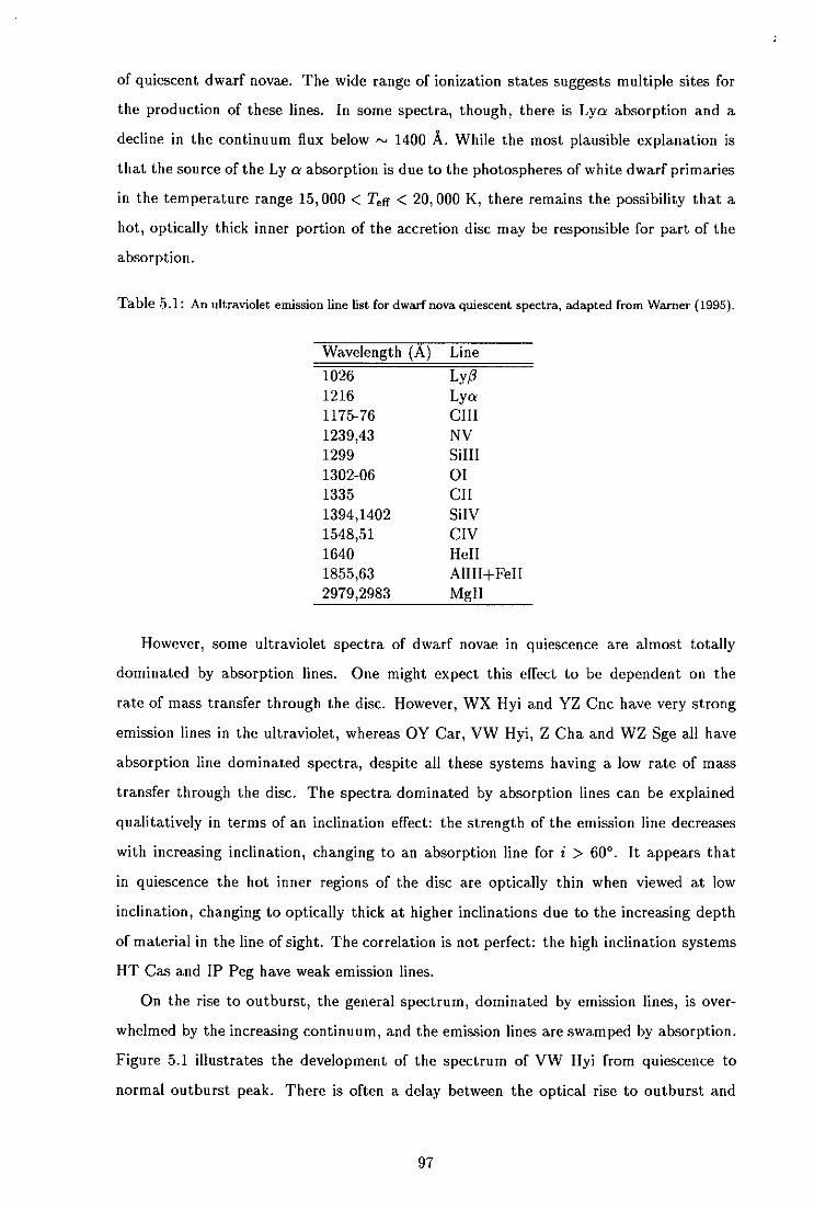
of quiescent dwarf novae. The wide range of ionization states suggests multiple sites for
the production of these lines. In some spectra, though, there is Lya absorption and a
decline in the continuum flux below r. 1400 A. While the most plausible explanation is
that the source of the Ly a absorption is due to the photospheres of white dwarf primaries
in the temperature range 15,000 < Tgj C 20, 000 K, there remains the possibility that a
hot, optically thick inner portion of the accretion disc may be responsible for part of the
absorption.
Table 5.1: An ultraviolet emission line list for dwarf nova quiescent spectra, adapted from Warner (1995).
Wavelength (A) Line
1026 Ly 1216 Lya 1175-76 CIII 1239,43 NV 1299 SillI 1302-06 0! 1335 CII 1394,1402 SiIV 1548,51 CIV 1640 Hell 1855,63 AIIII+FeII 2979,2983 MgII
However, some ultraviolet spectra of dwarf novae in quiescence are almost totally
dominated by absorption lines. One might expect this effect to be dependent on the
rate of mass transfer through the disc. However, WX Hyi and YZ Cnc have very strong
emission lines in the ultraviolet, whereas OY Car, VW Hyi, Z Cha and WZ Sge all have
absorption line dominated spectra, despite all these systems having a low rate of mass
transfer through the disc. The spectra dominated by absorption lines can be explained
qualitatively in terms of an inclination effect: the strength of the emission line decreases
with increasing inclination, changing to an absorption line for i > 60°. It appears that
in quiescence the hot inner regions of the disc are optically thin when viewed at low
inclination, changing to optically thick at higher inclinations due to the increasing depth
of material in the line of sight. The correlation is not perfect: the high inclination systems
HT Cas and IF Feg have weak emission lines.
On the rise to outburst, the general spectrum, dominated by emission lines, is over-
whelmed by the increasing continuum, and the emission lines are swamped by absorption.
Figure 5.1 illustrates the development of the spectrum of VW Hyi from quiescence to
normal outburst peak. There is often a delay between the optical rise to outburst and
97

N
N
Ln
(0 N
r-. N
3.1 3.15 3.2 3.25 log X
Figure 5.1: An illustration of the development of the ultraviolet spectrum of VW Hyi on the rise to
normal outburst maximum, as observed by the lifE in April 1990. The spectra (SWP40028 - 3WP40045;
from the JUEFA) were taken in sequence and clearly show the development of the continuum due to the
rise in flux from the disc, and the transition from a spectrum with emission lines to one dominated by
absorption lines. The Figure is plotted in log-log form because of the large rise in flux over the course of
the outburst.
the ultraviolet rise, although there are exceptions, e.g. CN On. While the propagation
of the transition front itself across the disc produces a delay, this is insufficient to explain
the observed delay durations. One of several explanations put forward for the ultraviolet
delay is that it is due to a refilling of the innermost regions of the disc, which may be trun-
cated due to irradiation by the primary (King 1997), or evacuated by a residual primary
magnetic field (e.g., Livio & Pringle 1992).
The appearance of the ultraviolet spectrum at outburst maximum is strongly depen-
dent on the inclination. For low inclination systems, the spectrum is dominated by ab-
sorption lines, with the exception of P Cyg profile emission, which is most often seen in
CIV A1550. For inclinations 70 0 < i < 80" the spectrum is almost featureless, while for
i > 80°, strong emission lines are seen.
The resonance lines in outburst are observed to have P Cyg profiles in many systems
with i < 65°, although the effect is by no means universal. Sometimes only the blue shifted
cI1

component of the P C yg profile is seen. These profiles are thought to be evidence for a
stellar wind during outburst; such winds are discussed further below.
Novalike variables
In general, the spectra of NLs display evidence for conditions of higher excitation than
those of dwarf novae, in keeping with the interpretation (within the framework of the
disc instability model) that these systems are similar to dwarf novae in a state of near-
permanent outburst. Differences are apparent, however, between novalike spectra and
those of dwarf novae at maximum. Additional lines of higher ionization are seen (e.g.,
Silil A1206, OV A1371). The dwarf novae do not develop the deep NV, SiIV and CIV
absorptions of the novalikes with optically thick discs, while emission lines appear strongly
in such novalikes for i > 65°, but only become strong in dwarf novae at maximum for
i > 75°.
5.3.2 Boundary layer temperatures from ultraviolet observations of CV
winds
Emission lines from CVs in the ultraviolet, specifically P Cyg profiles, can be used to
probe indirectly the temperature of the boundary layer region. This gives a very use-
ful alternative determination of this important parameter, allowing comparison with the
temperatures derived from X-ray observations.
It is the ultraviolet resonance lines in novalike variable spectra that show the most
compelling evidence for partial reversal into P Cyg profiles, implying, as with spectra of
dwarf novae in outburst, the presence of mass loss in a stellar wind. These winds are
thought, by analogy with the winds of early-type stars, to be driven by radiation pressure;
the P Cyg profiles of the ultraviolet resonance lines are formed by scattering in these winds
(Drew & Verbunt 1985). The second source of winds from CVs, the solar-type wind from
the secondary, has not yet been detected observationally. For a comprehensive review of
CV wind observations and models, see Mauche & Raymond (1997).
The differences between early-type stellar winds and those observed from CVs originate
in dissimilar wind geometries and discrete sources. In normal stars, the source for the
scattered continuum is the photosphere of the star itself; in CVs it is the accretion disc.
Furthermore, the presence of the accretion disc introduces a different wind geometry, and
an inclination dependence, as described below.
The lines most affected by P Cyg profiles in the JUE (and HST ) wavelength ranges
are the resonance lines CIV A1549, SiIV A1397 and NV A1240. The derived terminal

velocities of these winds (Va,) are comparable to the escape velocity from the primary
(— 5000 km r'), and it is only material from the inner disc, boundary layer region or
surface of the white dwarf itself that is likely to have been accelerated to these velocities
(Córdova & Mason 1982b). Mauche & Raymond (1997) list four reasons why accretion
disc winds are the more likely cause:
1. the gravitational potential at the surface of an accretion disc is much lower than that
at the surface of a white dwarf. This implies lower energies are needed to accelerate
the wind to escape velocity; -
2. the spatially extended nature of a disc wind has implications for the duration and
depth of eclipses of the line-forming region: the eclipses are often observed to be
shallow, indicating an extended zone;
3. spherically symmetric winds are observed to undergo an r 2 V(r)' density decrease
(where V is the velocity and r is distance). In a disc wind this decrease is likely
to be far less and the high-density component of the wind near the boundary layer
could be removed, allowing soft X-rays to emerge. This constraint also requires the
terminal velocity to be reached at a distance from the primary comparable to the
disc r&lius; and
4. lastly, since a disc wind will be produced in the same region as the region responsible
for the resonant scattering that produces the P C yg profiles, lower mass loss rates
are required for a given column density, and hence a given line strength, than those
required for a wind emanating from near the white dwarf.
As is the case in dwarf nova spectra, the P Cyg profiles are only seen in those systems
where i < 65°. This inclination dependence can be understood by considering a spherically
symmetric wind emanating from the centre of an accretion disc (e.g., Mauche & Raymond
1997). When the disc is viewed edge on, no part of the wind lies in front of the disc, so
all that is seen is the emission component whose full width is proportional to the terminal
velocity of the wind: Au = 2voVcc,/c. As the system inclination decreases, the fraction
of the wind seen in projection against the disc increases, giving rise to the absorption
component. At the same time, the strength of the emission component decreases. This
inclination effect is illustrated in Figure 5.2.
The ionization state of the wind is thought to be largely determined by the flux from
the boundary layer. Early investigations (e.g., Drew & Verbunt 1985; Kallman & Jensen
1985) encountered problems in explaining the ionization state of the wind within the
100

ME
W.
1.6 U)
a) -c 1.4
= 1.2 a)
-4-;
ca 1.0 a)
in
-2 -1 0 1 2 v/v..
Figure 5.2: Theoretical dependence of the strength and profile of the P Cyg feature on the inclination of
the system. When the disc is seen edge-on, only the emission component is seen; the situation is reversed
when the disc is viewed face-on, and only the absorption component is seen. From Mauche & Raymond
(1997).
framework of a classical (i.e. steady state) boundary layer and a smooth wind, where the
latter represented a mass loss rate that was a small fraction of the accretion rate. If these
assumptions are included in the models, the wind is ionized further than the observed
ionization states of NV, SiIV and CIV. Models by Mauche & Raymond (1987) predicted
some 100 times the observed Hell A1640 flux on the basis of these assumptions.
Hoare & Drew (1991) use the theoretical Zanstra (1931) method 5 to derive limits
on the boundary layer temperature of several novalikes and dwarf novae during outburst,
using the observed Hell .X1640 and .X4686 recombination lines. These lines occur if the
central ionising source is hotter than 50,000 K, and the observed strength of these re-
combination lines can be used to estimate the number of He+ ionizing photons produced
by the boundary layer flux. Because all the emission is assumed to come from the wind,
the derived boundary layer temperatures are upper limits. Their results suggest 50,000
TBL , 100,000 K.
Hoare & Drew (1993) followed up this work by constructing photoionization wind
models from discs with cool boundary layers (5 -9 eV) with the canonical mass flow rate
5 See Appendix A.
101

of M = 5x i0 M ® yr', and for discs with no boundary layer at all (i.e. primary rotating
near break-up speed). They then compared the ionization state of the winds predicted by
the models with those observed from spectra of low inclination novalikes (Hoare & Drew
1993). Their results implied that the observed strengths of the CIV and NV lines could be
matched by models with a cool, luminous boundary layer at 60,000 - 100,000 K, or disc-
only models (no boundary layer) where the accretion rate is 2-4 x 10⁻⁸ M ® yr'. In the
latter case the accretion rate was constrained by the need to have inner disc temperatures
of r's 7 x 10 K. The deduced mass loss rates from the wind were M w i nd 6 X 10 -10
M® yr', which appear to be reasonable values given the mass accretion rate and the
agreement with observed line strengths.
The temperatures derived from the Hoare & Drew studies are lower than the TEL
300,000 K boundary layer temperature expected from standard consideration of X-ray
production in the high accretion rate regime (see Chapter 1, Section 1.2), and suggest that
even if TBL = 300, 000 K, then the boundary layer luminosity can only be a small fraction
of the disc luminosity, another manifestation of the missing boundary layer problem. It is
not clear why this should be so. This discrepancy between the theory and the observation
of CV boundary layers has been a bone of contention since the very first X-ray luminosities
were calculated. The analysis of multiwavelength, multi-object observations by Howell et
al. (1999) suggests that, in all cases, high energy observations return high temperatures
and small emitting areas for the boundary layer, while ultraviolet and redward data return
lower temperatures and larger emitting areas. Howell et al. (1999) conclude that high
energy observations yield the best measurements of boundary layer temperatures because
the ultraviolet data is compromised by emission from the inner accretion disc.
5.4 The white dwarf primary
The accretion of matter onto the central object in a CV is a heating process, and as such
will delay the primary from suffering the eventual cold fate of an isolated white dwarf. In
addition to heating the white dwarf, accretion of matter from the secondary through a disc
also adds mass. This extra mass will have either solar abundances, or the abundances of
material processed from previous nova explosions, and will contribute angular momentum
to the white dwarf envelope. Thus studying the primaries in accreting CVs and the sub-
sequent comparison of these with isolated white dwarfs can provide illuminating insights
into the physics of the accretion process itself.
This Section is a summary of the use of ultraviolet spectroscopic observations to study
102
the white dwarfs in CVs. For an extensive, very recent, review of white dwarfs in CVs,
see Sion (1999); for an introduction to satellite observations of CV primaries, see e.g.,
Long (1999).
5.4.1 Detection
Ultraviolet light from a CV is typically dominated by that from the accretion disc. Cir-
cumstances fortuitously conspire, however, to allow the detection of the primary from
ultraviolet (and sometimes optical) spectra in three cases:
• in some dwarf novae with low mass transfer rates in quiescence;
• in some VY Scl novalike variables, where the mass transfer rate can drop temporarily
to reveal the spectrum of the primary;
• in some magnetic CVs during the low state, when the accretion appears to have shut
off.
For some years now the possibility of using ultraviolet spectra to parameterise the
primary (typically the temperature, the abundances of the accreted atmosphere and, more
recently, the rotational velocity) has been recognised. The first detections of primaries
came from observations of magnetic CVs during low optical brightness states when the
accretion appears to stop. Pioneering detections of photospheric light from the primary
of nonmagnetic CVs were carried out by Panek & HoIm (1984; U Gem), Mateo & Szkody
(1984; VW Hyi), Shafter et al. (1985; TT An) and others. Modelling of the newly-detected
primary spectra became an urgent priority.
However, in the case of CVs the modelling is not entirely straightforward because the
primaries are not isolated white dwarfs. They will be heated by the accretion process itself
and may preferentially be heated in the equatorial plane due to the boundary layer. In
fact, several high resolution HST Faint Object Spectrograph (FOS) observations of U Gem
by Long, Sion and collaborators have revealed evidence for an additional hot, possibly
equatorial, component at a considerably higher temperature than the white dwarf (e.g.
Long et al. 1993). Additional components are discussed further in Section 5.8.
The primary in a CV differs from a field white dwarf in another crucial respect: the
atmosphere is constantly accreting material from the accretion disc. In field white dwarfs,
the strong gravity drives a sedimentary process which causes the heavier elements to sink
towards the centre; at sufficiently low temperatures the structure of the white dwarf is
(theoretically) stratified, with a layer of nearly pure hydrogen on top of a layer of nearly
103

pure helium, and so on, through progressively heavier elements. The spectra of field white
dwarfs, therefore, have very little contribution from any elements other than hydrogen or
helium. To a very good approximation then, the ultraviolet spectra of field white dwarfs
can be modelled as pure hydrogen (DA type) or pure helium (DB type), with only trace
contributions from heavier elements. Note that there is considerable evidence for metal
absorbers in the atmospheres of high temperature white dwarfs (T0ff > 50,000 K), as
shown from optical follow-ups to the ROSAT WFC all-sky survey (Barstow et al. 1993;
Marsh et al. 1997). Marsh et al. found that all white dwarfs detected in the WFC all-
sky survey above Tff 55, 000 K contain metals in their atmospheres, and a steep rise
in opacity is seen at 54,000 K, which they interpreted as arising from the appearance of
radiatively supported Fe and Fe-group elements.
The CV primary, though, is likely to acquire a mixed-composition atmosphere through
the accretion process. Heavier elements may also be dredged up from deeper in the
atmosphere due to turbulent mixing driven by the shear of the boundary layer at the
equator. Solar abundance white dwarf spectra can thus be expected to provide better fits
to CV white dwarfs than pure hydrogen models alone.
5.4.2 Temperature determination of the primary
Background
Various heating mechanisms affect the white dwarf in a nonmagnetic CV. These include
(Sion 1999): instantaneously reradiated accretional heating, slow time-averaged release of
gravitational potential energy due to structure changes, angular momentum transport via
shear mixing and compressional heating. In shear mixing the rotational kinetic energy is
converted into heat and stored in the white dwarf for eventual release as a component of
surface luminosity. Sion (1999) states that the time-averaged surface luminosity L. and
temperature Teff for a white dwarf of mass and radius R, accreting at a time-
averaged accretion rate of At is:
L = L accg + Lsiiear + Lraci + L 00 i - (5.1)
where, as usual,
L3 1/4
Tff= 2 \4lrRWdcr)
(5.2) (
where L00j is the thermal cooling luminosity, Lrad is the luminosity due to the instanta-
neous reradiation of the accretion luminosity, L shear is the shear mixing luminosity and L
is the neutrino luminosity (from reactions in nova events). Laccg is the long term average
104

rate at which gravitational potential energy is liberated as a response to accretion and is
given by:
Laccg - fi (
GMWI GMdM\ - - Rd )
(5.3)
Here R OId is the Hamada-Salpeter (Hamada & Salpeter 1961) radius of a zero-temperature
white dwarf and 0 is the fraction of the total energy stored in the white dwarf. Then (1982)
modelled spherical accretion and showed that $ 0.15 - 0.25 of the total gravitational
potential energy difference.
As dwarf novae have typical outburst recurrence times of a few months, the primary
does not have a characteristic temperature as such: one would expect that the outer
layers of the white dwarf are heated to a certain temperature during an outburst and from
that point continue cooling down until the next outburst. At the same time, accreted
metals should diffuse towards the centre of the white dwarf, causing a change in the metal
abundance. Because of the cyclical nature of the accretion, derived surface temperatures
are thus an upper limit to the baseline (lowest temperature reached in quiescence before
another outburst) Teff value.
Observations suggest that white dwarf cooling is definitely detectable. In an example
relevant to this thesis, Gänsicke & Beuermann (1996) detail an investigation of the cooling
timescale for the white dwarf in VW Hyi after both normal outburst and superoutburst,
using modelling of IUE archive spectra with log g = 8 synthetic spectra. The cooling
timescale is the Kelvin time of the heated envelope layer:
Tic =ffYZdM r (5.4)
where c,, is the specific heat at constant volume, T is the temperature at the base of the
heated layer, L. is the luminosity and the integral is evaluated over the mass of the layer.
Gänsicke & Beuermann (1996) found that following an outburst, the accretion-heated
white dwarf cooled exponentially to a mean temperature of Tff c± 19,000 K. In addition,
they found that the cooling timescale was considerably longer after superoutburst (rs = 9.8
days) than after normal outburst (rpq = 2.8 days).
Strong evidence for the cooling of the white dwarf has also been found in observations
of U Gem. Long et al. (1994a) took two HST FOS observations of U Gem 13 and
70 days after the return, from the same outburst, to mean quiescent magnitude. During
this period of 57 days, the ultraviolet flux dropped by r.. 28% at 1400 A. This change is
much greater than the photometric variability and must therefore be considered as real
evidence for cooling. Long et al. then fitted synthetic white dwarf spectra to the data;
105

results suggested temperatures of 39,400 K for the first observation and 32,100 K for
the second. Further compelling evidence for a cooling of the white dwarf was given by
consideration of carbon and silicon spectral lines. The lines centred on Silli .X1260 A, SillI A1300 A and CII A1333 A were found to be weaker in the earlier spectrum. This is
important because, in a white dwarf photosphere, these lines are strongest at r'-e 30,000 K,
and weaken significantly as the effective temperature rises towards 40,000 K.
Another system in which the cooling of the white dwarf can easily be seen is WZ Sge,
a system that has very rare (each 33 years) outbursts which last approximately a month.
The most recent of these was in 1978, and the system was observed by JUE many times
over the years (1978 - 1992). The system is a unique laboratory for studying the cooling
of a white dwarf after outburst because of its long quiescence. Model fits to the quiescent
ultraviolet spectrum, which appears to have no disc contribution, show that the white
dwarf has been cooling ever since (Szkody & Sion 1989; Sion & Szkody 1991; Sparks et
al. 1993). The last JUE spectrum of WZ Sge was acquired in 1992; subsequent HST FOS
observations have allowed more accurate temperature determinations to be made for the
white dwarf (e.g., Sion et al. 1995c, who find Td = 14, 800 K), and have allowed the
estimation of abundances in the primary photosphere.
These observations present compelling evidence that, in these low Al systems, the
white dwarf is cooling down during the quiescent periods.
Temperature determination methods
There are several methods that can be employed to estimate an average temperature for
the white dwarf in a CV. Among the first to be used were eclipse depth measurements.
For this method, photometric light curves of high-inclination systems are decomposed
into their component parts (e.g. Wood et al. 1985) and the flux of the white dwarf
component measured across a range of different passbands (e.g. U, B, V, R). Blackbody
approximations or white dwarf model atmospheres are then fitted to these points. The
application of this method is obviously limited to eclipsing systems; in addition, it suffers
from the restriction that one can only have as many points as one has passbands, leading
to poor temperature discrimination. However, it does have the advantage of removing
any disc contributions. Generally, primary star temperatures deduced from this method
are cooler than the temperatures derived from ultraviolet data, perhaps reflecting the
fact that the white dwarf radiates primarily in the ultraviolet spectral range. Examples
of temperature determinations of the white dwarf in OY Car using infrared and optical
photometry can be found in Berriman (1987) and Wood et al. (1989). Berriman found
106

10,000— 15, 000 K, while Wood et al. found 15,000 K.
In the case of ultraviolet spectra, fits to the Lyman a line and ultraviolet continuum
can give a reasonable temperature estimate in those systems where the spectroscopic
signature of the primary can be identified and there is minimal disc contribution. Broad
Ly a absorption is indicative of a cool primary; the hotter the white dwarf is, the narrower
the Ly a absorption (see Figure 5.3).
0
Co
oc2 x
Co
E 0
a' o X
c..l
'C I
n
1200 1300 1400 1500 1600 1700 1800 1900
Wavelength (A)
Figure 5.3: Synthetic solar abundance ultraviolet spectra for Teff = 16,000 K (light grey) and Tetr =
20,000 K (black), illustrating how the Lyman a absorption profile narrows with a hotter white dwarf.
Both spectra cover the ILIE wavelength range, have been convolved with a Gaussian of FWHM 6 A to
match the JUE wavelength resolution, and resampled to the JUE binsize.
The results are potentially far more accurate than those from optical eclipse depth
measurements. The fitted spectra may be the spectra of field white dwarfs (e.g., Hassall
& Ia Dous 1996), or more sophisticated model fits such as those by Sion, Long, Hubeny and
collaborators (e.g. Long et al. 1993; Sion et al. 1995), or the Kiel group (e.g. Gänsicke
& Koester 1999). Warner (1995) lists 27 nonmagnetic CVs where temperatures have
been derived for the white dwarf. The mean temperatures from the best determined
measurements (i.e., synthetic spectral modelling), are 50,000 K for novalikes and 19,200 K
for dwarf novae, which is (unsurprisingly) higher than the median temperature of 10,000 K
107

for field white dwarfs (Sion 1984).
5.4.3 Other measurable primary parameters
Rotational velocities
Quantitative estimates of the global rotational velocities of CV white dwarfs have only
been possible since the advent of the high resolution spectra available from the HST and
the Hopkins Ultraviolet Telescope (HUT). Field white dwarfs are as a rule slow rotators:
Heber et al. (1997) establish an upper limit for the rotation rate of DA white dwarfs of
usin i < 40 km r'. But white dwarfs in CVs are accreting material. High resolution HST
FOS and HUT spectra have allowed questions concerning the amount of angular momen-
tum transferred to the white dwarf due to the accretion process to be addressed. Other
questions, such as whether the white dwarfs in CVs are rotating near breakup velocity
and hence would explain weak or missing boundary layer flux, can also be addressed. The
resolution of the JUE spectra is insufficient for this type of analysis.
Values for the rotational velocity of 8 CV white dwarfs are listed in Sion (1999). The
values found range from 1200 km s 1 for WZ Sge (Cheng et al. 1997b) to < 100 km
in the case of the white dwarf in U Gem (Sion et al. 1994). Since the time-averaged
accretion rate of a CV white dwarf is— 10 10M® yr 1 , and a typical CV lifetime is io
yr, this implies that most CV white dwarfs should be rotating near breakup (e.g., Sion
1999, and references therein).
However, on the basis of the 8 rotational velocities so far derived, only WZ Sge is
rotating at anything like this velocity: the white dwarf in this system is rotating at ". 30%
of breakup (Sion 1999). WZ Sge is generally acknowledged to be an exceptionally old
system, aged r-' 109 years (Sion et al. 1995b), and it has the fastest white dwarf rotational
velocity yet found.
To explain slow rotational velocities, earlier models invoked ejecta from nova explosions
taking angular momentum away from the white dwarf. While this is still viable, the effect is
too small to explain the quantitative results now available. Instead, Livio & Pringle (1998)
suggest that the common envelope phase of the nova is capable of braking the primary
rotation rate in relatively old CVs. In this scenario, shear between the surface of the
primary and the bottom of the convective envelope generates a magnetic field of sufficient
strength to exert the torque needed to slow the white dwarf.

Chemical abundances
Estimates of the metal abundances in CV white dwarfs have also only been possible
since the advent of the high signal to noise spectra available from HST and HUT. The
white dwarfs in CVs can and do display spectroscopic features with abundance ratios and
chemical species that cannot have an origin in accreted matter from a normal secondary
star: these can provide important clues to the evolutionary past of the system and of the
white dwarf itself.
Chemical abundances of 8 CV white dwarfs have been reported up to the time of writ-
ing, primarily from analysis of HST FOS spectra (see Sion 1999, Table 7). These systems
display a wide range of overabundances and underabundances. The Sion et al. (1997)
analysis of VW Hyi determined a N abundance far in excess of the abundances of C and 0,
and even more interestingly, discovered elevated levels of P and Al (P at 900 times solar!).
Sion et al. interpret these abundances as evidence for a prehistoric nova outburst in VW
Hyi: P and Al are products of proton capture nucleosynthesis which takes place during a
thermonuclear runaway. Interestingly, theoretical calculations for the diffusion timescale
in the atmosphere of a white dwarf similar to that seen in VW Hyi yield timescales of
3-4 days. Sion et al. (1997) interpret the fact that P is seen at all as being evidence for
dredge-up due to shear mixing with the accretion belt observed on the white dwarf in
quiescence. This may also explain why changes in the chemical abundances have not been
detected in observations obtained at different times after the same outburst.
Sion et al. (1998a) find a subsolar C abundance for the white dwarf in U Gem, which
they also attribute to an ancient thermonuclear runaway event. The justification runs thus
(Sion 1999): During a thermonuclear runaway, C captures a proton to form N. The more
supersolar the C, the stronger the thermonuclear runaway (Starrfield 1993); the supersolar
C abundance comes from mixing of the accreted material with white dwarf core material
(Starrfield et al. 1972). If there is no core mixing, then the thermonuclear runaway will
be weak. In a slowly accreting white dwarf (such as a dwarf nova), the thermonuclear
runaway is relatively weak, little material will be ejected from the system, and a large
common envelope will form. Some of this envelope will be ejected, but a large fraction will
be deposited on the secondary and a similar fraction will be consumed in the H-burning
shell around the white dwarf which has been rekindled by the thermonuclear runaway. This
shell will leave a He-rich layer enriched in N and depleted in C. Subsequent thermonuclear
runaways exacerbate the C depletion. Later dwarf novae deposit C-depleted material due
to the thermonuclear runaway and common envelope, to be mixed with even stronger
109

C-depleted white dwarf material due to the thermonuclear runaway and the remnant H-
burning shell source. This complex explanation leads to a C-depleted and N-enhanced
white dwarf photosphere, which has been observed (Sion et al. 1998a, Long & Gilliland
1998). There is a necessarily speculative element, but assuming that present theories of
CV evolution are correct, the model plausibly explains the observed abundances by placing
them within the current evolutionary framework.
Abundance determinations, then, can yield important information concerning the his-
tory of a given system, provided the white dwarf is visible. There is further discussion of
this subject in Section 5.8
5.4.4 Summary
The preceding Sections have detailed the use of ultraviolet spectroscopic investigations to
estimate various CV primary star parameters.
What follows is an investigation of the modelling of ultraviolet spectra, examining
how the method may be honed to obtain the best possible results from the upcoming
HST data. Because of the great number of spectra available in the IUEFA, much of the
investigation concentrates on IUE ; however, some HST FOS spectra, notably those of
OY Car itself and VW Hyi, are also modelled.
5.5 Spectrum dearchival and initial development of the fit-ting process
In dearchiving CV spectra from the LUEFA with a view to modelling the Lyman a region
and ultraviolet continuum, certain selection criteria had to be imposed. These included:
Only SWP (1150- 1950 A) spectra were dearchived as the disc contribution usually
rises to unacceptable levels in the LJWP/LWR (1900 - 3200 A) spectra6 .
• Those spectra with the lowest flux levels were then needed, as these will have the
least disc contribution. Some of these spectra were the result of poor acquisition, so
these were excluded on grounds of quality.
• Only dwarf nova spectra were dearchived as these objects are the main subject of
this work.
As a starting point, the catalogue of IUE spectra of dwarf novae and novalikes assem-
bled by Ia Dous (1990) was used, which lists all dwarf nova spectra obtained by IUE up
° Although see Gänsicke & Koester (1999), in which the entire SWP/LWP spectrum of CU Vel is convincingly modelled with a Tee = 18500 K, log g = 8 synthetic spectrum. This is unusual.
110

to 1987. In some cases the selection of the lowest flux spectrum was complicated by poor
quality low flux spectra caused by bad centering of the star in the aperture, inadequate
exposure times or poor trailing by the satellite during the exposure. Table 5.2 lists the
lowest flux DN spectra dearchived from the Ia Dous (1990) catalogue; thumbnail plots of
these spectra can be seen in Figures 5.4, 5.5 and 5.6. For those low 1* systems where the
primary contribution was clearly seen, the whole data set was subsequently dearchived.
The initial aim was to develop a simple program that would optimise the fitting of
field DA white dwarf spectra to those of quiescent dwarf novae, thus yielding a first
approximation of the temperature of the primary. To this end, some 57 JUE field DA
white dwarf spectra with well determined temperatures were dearchived. The white dwarfs
themselves were chosen from a preliminary version of an atlas being developed by Sion
and Ia Dous (La Dous, private comm.). This procedure contributed to familiarisation with
the IUEFA interface and dearchival procedures, in addition to white dwarf spectra in the
ultraviolet.
Each spectrum was converted from the initial FITS format to an ASCII file using a
publicly available conversion program (mxconv2.osf) written by Dr. M. Currie at UCL
(available from http://www.star.ucl.ac.uk/ mj c/iuedr/iuef a .html). Some of the
files were also converted using the STARLINK CONVERT package as a check of the reliability
of the conversion program. Results were exactly the same in each case. The output is in
the form of a six-column table: the wavelength (A), the absolute flux (fx), net flux
background flux (IA), flux error, and a quality flag.
The low flux dwarf nova spectra were then individually compared to the atlas of white
dwarfs, and the best fitting white dwarf spectrum was selected by the use of the reduced
x2 statistic7 , and which for these exploratory purposes was evaluated across the whole
JUE SWP wavelength range: 1150 - 1950 A, except for a 20 A region centred on Ly
a. The errors on each IUE spectrum are of the order of 10%; see Figure 5.7 for an
illustration. Any data points flagged as bad quality were excluded from the fit. In those
cases where a white dwarf was visible in the CV spectrum, the results agreed relatively
well with published values of the primary temperature where available, giving temperature
determinations that were generally consistent to within ±3000 K in all cases.
The WZ Sge post-outburst dataset can be used to illustrate that temperature discrim-
ination is even possible with this rudimentary white dwarf spectrum-fitting method. The
first "quiescent" post-outburst spectrum of WZ Sge was best modelled with a spectrum
7 Notation x The x2 statistic is defined in eqn. 2.8. x = x2 /v, where ii is the number of degrees of freedom (the number of data points minus the number of parameters to be determined from the data points).
111

corresponding to a white dwarf at Teff r. 25,000K. The subsequent spectrum, acquired
almost exactly six months later and by now more clearly exhibiting the Lya absorption
expected for a white dwarf, was best modelled with a spectrum corresponding to a white
dwarf at Teff r.s 17, 000 K. Figures 5.8 and 5.9 illustrate these fits. Obvious areas of poor
fit are in the absorption lines due to the solar composition of the white dwarf photosphere,
especially in SiIII A1300, CII A1335, SiIV AA1394, 1403 and CIV AA1548, 1551. In addi-
tion, and for later comparison, Figure 5.10 is a plot of x3 vs. white dwarf temperature
for the latter fit, and shows quantitatively the temperature discrimination available when
fitting field white dwarf spectra to those of CVs.
The validity of the procedure and program now having been established, more detailed
and realistic modelling was undertaken, which is described in the following Sections.
112

Zi
ti 91
(xfl)&
1
Li- T
fl- tL
9ti-
(xnIj)o
1
Zi
Li-
tV
(xnu)o
1
Li-
(xnu)o
1
Li-
t1
ci-
(xnu)o
1
cii-
i
Tfl- L
i
ci-
ci-
ti (x
nij&
ri (x
nu)&
1
C
'$ 0
0
V
0)
— >
4
0
EZ
O
2 S
E-
a)
a) -
a)>
C
'o
L
.0
u
Q
UN
V
a) V
C v
C
V
'C
o
1)
0
a
• I : -c
0
3
Cu
o
a)
a)' C
V
0
a) a
C) r)
tt
E
a) a)a)
a)
'• U
I-
113

E 0
CL-
H-
tV
CL-
tL
cL-
ZN
C
1 t1
Q
L (x
nu
)o1
(n
u)6
o1
(xn
i4)b
oi
a
C
LI-
Q
tL-
CL-
GC
1 (x
flu)b
ol
(xnhj)Oo1
(xrqJ)o
1
I
>
U
0
to
ttO
V
V (
t V
I-
bO
ctI-
L
I- (n
u)b
oi
ZN
LI-
(xN
jo1
ZN
L
V tV
G
L-
(xnu)b
Di
114

8 N
(xflIj)O
1
(xn
hJ)o
1
a-
I
8 N
C
0
0
0I
(xn
u)6
o1
.E •
0)
0) @
) C
) V1
0.
II 4)
Ii. -c
4 r/)
I -
V
U
c V
--
c
-a bO
-C
-
- 4) @
0.
-WE
E
00 C
: &
0.)
Co
C
- C
C" C
E
C >
E
U
0) 4
)
bC
CC U
V
0
V
U)
I. 4
)0
)4
)
0
0V
C
o
C
0<
- —
U
bjO
11
5

2e-13
l.5e-13 2 U, 0
le-13
LI-
Se-14
El 1200 1300 1400 1500 1600 1700 1800 1900
Wavelength (Angstrorns)
Figure 5.7: A spectrum of VW Flyi in quiescence (SWPI09I1), illustrating the typical extent of the
errors in an JUE spectrum, as calcuiated by the NEWSIPS extraction process.
Table 5.2: A list of the most quiescent dwarf nova spectra (good quality spectra having the lowest flux)
obtained from the IUEFA. Asterisks indicate a system for which the whole data set was dearchived; the
stars are listed in the alphabetical order of their respective constellations.
Object Spectrum Object Spectrum
RX And 5WP17642 U Gem SWP24716 SS Aur 5WP16036 AH Her SWP08089 Z Cam SWP18844 VW Hyi* SWP23865 OY Car 5WP28263 WX Hyi SWP09704 HT Cas SWP21080 T Leo SWP27683 BV Cen SWP03857 CZ Ori SWP16042 Z Cha* SWP30780 V2051 Oph SWP21091 HL CMa SWP22211 RU Peg SWP28449 YZ Cnc SWP07312 WZ Sge* SWP31294 SS Cyg 5WP24533 EK Tra SWP09768 AB Dra SWP07413 SU UMa SWP18845
116

SWP03768_scr.dat
0
(P17 0
C.,
E C.)
P.,
t._ 0 a)-
LJ eC
0
5'c1O'
0
—5xIC' 3
1200 1300 1400 1500 1600 1700 1800 1900
Wavelength (A)
Figure 5.8: The first "quiescent" post-outburst spectrum of WZ Sge (SWP03768; grey), modelled with
the spectrum of a field white dwarf at a temperature of Tee 25,700 1< (SWP17014; black). The X2 = 3.4.
Residuals are plotted (not to the same scale) in the bottom panel.
SWP057 44_sc r. dat
0
0
—1 1200 1300 1400 1500 1600 1700 1800 1900
Wavelength (A)
Figure 5.9: The spectrum subsequent to that in Figure 5.8 (SWP05744), obtained six months after,
modelled with the spectrum of a field white dwarf at a temperature of T5 — 17,000 K. The x = 2.4.
The field white dwarf spectrum (SWP07973) is again black. Residuals are again plotted, not to the same
scale, in the bottom panel.
117

30
25
20
g
15
10
5
0
'chisq.dat' 0
0 0
0
0
0 00 0
00 0 0 0
0 0
0
0 0
0
0 0 0
0
0 0 0
00
0 Co
Co 0
10000 20000 30000 40000 50000 60000 70000 Temperature of white dwarf specinim
Figure 5.10: The JUE spectrum of WZ Sge (SWP07973) has been fitted with field DA white dwarf spectra
in the temperature range 10,000 - 70,000 K. The x vs. white dwarf temperature plot for the sequence of
fits is shown above. It can be seen that there is a clear, but broad, minimum in the x2 -distribution centred
around Tes 17,000 K. This fit is shown in the previous Figure ( 5.9). For comparison with the similar
plot obtained from a synthetic spectral fit to the same WZ Sge spectrum (Figure 5.15).
118

5.6 Model construction using TLUSTY and SYNSPEC
Section 5.5 showed that approximate effective temperature determinations for the primary
star could be achieved by simply fitting the observed spectrum of a field white dwarf star
to that of a quiescent dwarf nova. The main problem with the method is the inappropriate
abundances of field white dwarf spectra when applied to the analysis of CV primary star
spectra. It is also useful to have a regular grid of different temperature spectra with which
to analyse the CV data, rather than the unevenly spaced grid of variable quality spectra
available from field white dwarf observations.
In order to improve the effective temperature estimates for the primaries in the sample,
and to provide a reliable measure of the quality of the fitting, several grids of white dwarf
model atmospheres and synthetic spectra were calculated.
For a review of the development of stellar atmosphere computations, see e.g. Kudritzki
& Hummer (1990), or Werner & Dreizler (1999). Kudritzki & Hummer define the photo-
sphere of a star in the context of stellar atmosphere models: it is " ... that part of a star
in which radiative equilibrium and hydrostatic equilibrium hold but the Saha-Boltzmann
and Planck distributions cannot be assumed". The structure of the photosphere of a star
is determined not only by radiative and hydrostatic equilibrium, but also by the radiative
transfer equation and by the condition of statistical equilibrium, which requires the num-
ber of transitions into and out of each atomic level to be equal. To calculate the model
atmosphere, an equation of state (usually the ideal gas law), the elemental abundances,
and the geometry of the atmosphere must be specified, in addition to the collisional and
radiative cross sections and rate constants. For a review of the basic equations used in
the calculation of model atmospheres and synthetic spectra, see Appendix B.
All model atmosphere codes work in approximately the same way. This involves si-
multaneously solving the basic equations of radiative transfer, hydrostatic equilibrium,
radiative equilibrium, particle conservation and statistical equilibrium. The model atmo-
sphere itself is then a set of tables of e.g., the source function and/or temperature vs.
pressure and/or optical depth.
In order to solve the basic equations, several simplifying assumptions are necessary.
These include:
• the assumption of plane parallel geometry, which streamlines matters considerably
as all variables are then a function of only one spatial coordinate. This assumption
is valid when the mean distance between the emission and the next absorption or
scattering of the photons is very small compared with the stellar radius at that point;
119

• that the atmosphere is in radiative and hydrostatic equilibrium. If this is the case,
no large scale accelerations occur;
• that there are no starspots, granulations or prominences, or gas flows in any direction
other than radial (a manifestation of the plane parallel assumption); and
• that there are no magnetic fields.
Early model atmospheres (pre-1970) also assumed, for simplicity, the condition of local
thermodynamic equilibrium (LTE) holds; that is:
. that the spectral density of the radiation is described by the Planck function;
• that the total energy density of the radiation is described by the Stefan-Boltzmann
Law;
• that the velocity distributions of the atoms, ions and electrons is described by the
Maxwell-Boltzmann distribution; and
• that the atomic-level populations are specified by the Saha-Boltzmann equations at
the local electron temperature.
The computational technique that made it possible to abandon the assumption of LTE
was "complete linearization", introduced in 1969 by Aeur & Mihalas. They demonstrated
that models based on statistical equilibrium produced spectra that agreed substantially
with observations, where LTE models had always failed to do so. These statistical equi-
librium models, often termed non-LTE (NLTE), differ from LTE models in that the pop-
ulations of some selected energy levels of some selected atoms and/or ions are allowed to
depart from their LTE values.
There are many different model stellar atmospheres available, perhaps the most famous
of which in the astrophysical community are the LTE models from ATLAS, by Kurucz, first
published in 1970. Up to date versions of the Kurucz model atmospheres and synthetic
spectra are currently available on CD ROM or from http :1/cf aku5 . harvard. edu/. There
is also the Kid code, written over 20 years primarily by Dr. D. Koester (see, e.g. Dreizler
& Werner 1993; Finley et al. 1997).
This Chapter will use the programs TLUSTY and SYNSPEC, written by Dr. I. Hubeny
and collaborators, which are extensively used by Sion, Long et al. in the modelling of
ultraviolet/EUV spectra of CVs.
120

5.6.1 The basics of TLUSTY
For the original detailed description of TLUSTY, see Hubeny (1988). The code has
undergone a considerable number of revisions and upgrades since original publication; the
major new developments are described in Hubeny & Lanz (1992), Hubeny et al. (1994)
and Hubeny & Lanz (1995).
The latest version of TLUSTY (TLUSTY195) uses a computational method known as
the hybrid complete linearization/accelerated lambda iteration (hybrid CL/AL!; described
in Hubeny & Lanz 1995 and Werner & Dreizler 1999), an evolution of the original complete
linearization method first introduced by Aeur & Mihalas (1969).
In essence, the CL method allows the discretisation (by depth and frequency) of the
nonlinear and strongly coupled equations describing the atmosphere. These equation can
then be solved iteratively using a set of linear equations for corrections to the values of
all quantities (temperature, atomic-level populations, densities and the intensity of the
radiation at each frequency) from the previous iteration (Kudritzki & Hummer 1990).
This method gives a fast convergence rate.
The AL! method is conceptually based on work by Cannon (1973b) and Rybicki (1972),
was reformulated by Scharmer (1982), and was first applied to the construction of model
atmospheres by Werner (1986). The basis of the AL! method is to express the radiation
intensity through an approximate ("lambda") operator operating on the source function,
plus a correction term known from the previous iteration. This reduces the time per
iteration and thus increases the speed of computation.
Fully line-blanketed NLTE models are available using TLUSTY195; this is achieved by
introducing the concept of "superlevels". The term line blanketing involves the study of
the influence of the thousands to millions of spectral lines on the atmospheric structure and
emergent spectrum. Despite the combination of fast convergence rate and reduced time
per iteration introduced by the hybrid CL/ALl method, its use is limited, because each
energy level is treated separately. This effectively means that atoms with a very complex
energy level structure, such as the iron-peak elements, cannot be treated. To overcome
this limitation, TLUSTY195 uses the approach of Anderson (1989), in which the problem
of radiative transfer in the millions of atomic transitions is addressed with a statistical
solution based on grouping many energy levels into a small number of "superlevels".
TLUSTY195 is an extremely flexible piece of code. It solves the basic equations (ra-
diative transfer, hydrostatic equilibrium, radiative equilibrium, particle conservation and
statistical equilibrium); the program has options for calculating semi-empirical models
121

where the temperature distribution is fixed and all other equations are solved exactly. It
is fully data oriented with no built-in opacity values, and it is highly portable, having been
written in Fortran 77.
Output files are in the form of H. vs. wavelength, where H,, is the first moment of the
specific intensity and is defined in e.g., Cray (1992; see also Appendix B).
TLUSTY (Hubeny 1988) is the basic plane-parallel, horizontally homogeneous model
stellar atmosphere calculation program. Departures from LTE are allowed for selected
atomic and ionic energy levels, and the program also incorporates convection (based on
the mixing-length formulation). Version 195 allows fully consistent NLJTE metal line blan-
keting. The most up to date versions of these programs are available from Dr. 1. Hubeny
himself. The older version TLUSTY185 is available for download from the TLUSTY
home page at http://tlusty.gsfc.nasa.gov . The still older versions TLUSTY178 and
SYNSPEC36 are also distributed by the CCP7 Project (http://ccp7.dur.ac.uk ).
Associated programs
The companion program is SYNSPEC (Hubeny et al. 1994; now at version 42), which
calculates the spectrum emergent from the model atmosphere (SYNSPEC can also take
Kurucz model atmospheres as input). If the input model atmosphere was calculated in
LTE, then SYNSPEC assumes the source functions for the continuum and lines is given
by the LTE value, i.e., the Planck function. If, however, some of the atomic energy levels
depart from LTE, then the lines from these levels can be calculated using an NLTE source
function. SYNSPEC includes two kinds of NLTE treatment of the line source function:
exact NLTE; and approximate NLTE. The latter assumes that the source function is
given by an analytical expression derived from second-order escape probability theory
(e.g. Hummer & Rybicki 1982).
A further program, CIRCUS (unpublished, version 1) calculates stellar spectra under
the influence of external emitting or absorbing bodies, i.e. veiled spectra. Each cir-
cumstellar body is assumed to be an homogeneous, isothermal slab, characterised by its
geometrical parameters (including column density, radial velocity, relative projected area
and position), and physical parameters (including temperature, electron density, mass
density and velocity dispersion). Additionally, each body may absorb or emit radiation.
Convolutions of the resulting spectrum with the rotational profile and/or the instru-
mental profile are achieved by the use of the program ROTIN (unpublished; now at version
4).
For a summary of the various input and output files and optional parameters available,
122

with examples, see Appendix C.
5.6.2 Calculating the model atmospheres and synthetic spectra
Once TLUSTY195 and SYNSPEC42 were downloaded and compiled at Preston, some
tests were undertaken to ensure that the programs were in working order, using sample
input and output files supplied with the codes for this purpose. It was first found to be
necessary that the instantaneous data storage capacity at the disposal of the program be
expanded in order to run these programs on the Preston STARLINK node, not surprising
considering the line list contains more than 185,000 lines in the SWP spectral region.
Several program arrays also had to be extended.
Because of the complex format and arrangement of input and output (I/O) files (see
Appendix C), and the necessity of renaming the output files to prevent overwriting by a
subsequent run, it was found easiest to run TLUSTY and SYNSPEC using a new front-
end written by the present author as a UNIX C-shell script. C-shell scripts introduce a
large amount of flexibility into the running of TLUSTY and SYNSPEC, giving complete
control of the I/O files (including renaming on completion of a run), and permitting the
batch processing of jobs to be undertaken in a relatively painless fashion.
All of the following model atmospheres were calculated in LTE only, with an approx-
imate NLTE treatment applied to the calculation of the resulting synthetic spectrum. At
the temperaures and gravities in question here, departures from LTE have been shown
by other studies to have negligible effects on both the structure of the atmosphere or the
resulting synthetic spectrum as produced by these programs (Long et al. 1993; Home et
al. 1994). Lanz & Hubeny (1995) provide a detailed discussion of NLTE effects in hot,
metal-rich white dwarfs: NLTE effects become important at temperatures of > 60,000 K.
Figure 5.11 illustrates the difference between synthetic spectra resulting from calculations
using LTE and approximate NLTE treatments. The continuum level and slope, and the
Lyman a line are almost unaffected; some lines are deeper in the NLTE spectrum, but
line depths are unimportant in this analysis. Differences between LTE and NLTE are
undetectable at IIJE resolution.
Pure H/He model atmospheres and synthetic spectra
Pure H/He models were the first to be produced for the present work. These model
atmospheres composed of pure hydrogen and helium in their solar abundances, were the
first to be produced. These so-called "pure hydrogen" models (with logg = 8) have been
very successful in the past when applied to the determination of the temperatures of field
123

0
x N
an
1200 1300 1400 1500 1600 1700 1800 1900
Wavelength (A)
Figure 5.11: An illustration of the difference between an LTE spectrum produced from an LTE model
atmosphere with that produced from the same model atmosphere but using an NLTE approximation (red).
The spectrum covers the JUE wavelength range and has been convolved to JUE instrumental resolution
and resampled to the JUE binsize.
white dwarfs. Log g = 8 models are generally used as a simplification: the gravity is then
a fixed parameter corresponding to a canonical Md 0.6M® white dwarf. The effect of
the white dwarf mass on the final calculated spectrum is discussed further in Section 5.8.
When utilized in the context of lUll spectra of CVs, pure H/He models allow an al-
ternative approach, in that the estimate of the effective temperature of the primary is not
limited by the signal to noise of field white dwarfs, as described in Section 5.5. The gen-
eration of these relatively simple models was a useful step in the process of familiarisation
with calculating model atmospheres and synthetic spectra using TLUSTY and SYNSPEC.
A grid of H/He-only, logg = 8, LTE model atmospheres was generated in the tem-
perature range 14,000 - 50,000 K, with appropriate increments in Tff. The models were
initially produced on a very fine wavelength scale (SA = 0.1 A). it was found that models
with Teff < 15,500 K would not converge with a "standard" TLUSTY input file. This is
because convection becomes progressively more important as a means of energy transport
at lower temperatures. A special set of "cool" input files, incorporating convection, was
124

x UI
ci,
E 0
aZ L. I 0) 0
-c Li
an
1200 1300 1400 1500 1600 1700 1800 1900
Wavelength (A)
Figure 5.12: An example of an H/He synthetic spectral fit to the quiescent JUE spectrum of VW Hyi,
at Tes = 18000 K. The Ly a absorption and the shape of the overall continuum is very well described,
but individual features from heavier elements are (obviously) not.
thus obtained in order to generate model atmospheres with Teff , 15,500 K (Hubeny,
private comm.). The final synthetic spectra were produced from the model atmospheres
using SYNSPEC, then convolved with a Gaussian of suitable FWHM to match the resolu-
tion of JUE using the rotational and instrumental convolution program ROTIN4; values
for the J(JE resolution (r.J 6 A FWHM mean) were obtained from the ESA IUE Newsletter
Figure 5.12 shows an example H/He synthetic spectral fit to a quiescent spectrum
of VW Hyi. In common with the white dwarf spectral fits described in Section 5.5, the
Lyman a region and the overall shape of the continuum are very well described, but fits
to individual lines (non H/He) are obviously not possible.
Solar abundance model atmospheres and synthetic spectra
A grid of solar abundance, log g = 8 model atmospheres was next generated. Long, Sion
and collaborators use H and He as the continuum opacity sources when calculating the
structure of the model atmosphere, the rationale being that at the temperatures and
125

gravities of interest in the study of white dwarfs, metals do not affect the opacity of the
atmosphere significantly. However, for the calculation of the solar abundance synthetic
spectra used here, hydrogen, helium and carbon were used in the calculation of the model
atmospheric structure. This was the approach taken in the model atmosphere calculations
in Home et al. (1994). The neglect of full metal line blanketing on the final calculated
spectrum is discussed further in Section 5.8; Figure 5.25 in that Section illustrates the
temperature difference that results from the inclusion of C.
Synthetic spectra for the JUE spectral range were then produced using SYNSPEC,
covering an effective temperature range of T0ff = 14,000 - 50,000 K, with appropriate
increments in T0ff. The source functions of the resonance lines for the first 20 elements (H
- Ca) were calculated using the approximate NLJTE option, while an LTE source function
was assumed for all other transitions (cf. Home et al. 1994). The intrinsic line profiles
have the form of a Voigt function and account for the contributions of natural, van der
Waals, Stark and thermal Doppler broadening. As with the H/He synthetic spectra, a
very fine wavelength grid was used initially (5A < 0.1 A) ; the spectra were then convolved
with a Gaussian of FWHM equal to JUE instrumental resolution (6 A) and resampled to
match the JUE bin size.
Veiled spectra
Finally, veiled spectra were calculated using TLUSTY, SYNSPEC and CIRCUS. The pro-
cedure for calculating these spectra was quite complicated. Firstly, normal solar abundance
white dwarf spectra were produced in the usual way in the temperature range of interest.
In this case, spectra were generated in the temperature range T0ff = 14,000 - 25,000 K,
with appropriate temperature increments. Next, a grid of opacity tables was produced
for absorbing bodies at temperatures of T0ff = 7500, 10,000 and 12,000 K, and column
densities of NH = 1020, 1021 and 1022 cm 2 . The models assume a uniform density slab for
which an electron density of it0 = 10 13 cm 3 has been chosen, in keeping with the values
found in the Home et al. (1994) study. Obviously this is a gross simplification: a realistic
model would utilize a density gradient and a more realistic geometry, but the inclusion
of these factors is beyond the scope of the present work. It will be seen that order of
magnitude results are possible with these simplifications. These calculations required the
use of the 'iron curtain' mode of SYNSPEC, which calculates monochromatic opacities for
a homogeneous slab of a given temperature and density. The spectral files and the opacity
tables were then used as input to CIRCUS, which calculates the resulting spectrum after
absorption by the circumstellar body. Figure 5.13 illustrates the effect of the veiling gas
126

on a Teff = 16, 000 K logg = 8 synthetic spectrum.
As a result of the various assumptions used here, the temperature and column density
uncertainties on any fits to 'iron curtain' spectra are 2,500 K and a factor of ten, respec-
tively. The proposed improvements to the method to lessen the uncertainties are discussed
in Section 5.7 and Chapter 6.
0
x
0 Co -
E C)
N
32 .- 'C
in
I
1200 1300 1400 1500 1600 1700 1800 1900
Wavelength (A)
Figure 5.13: A comparison of an unobscured T0 = 16,000 K, logy = 8 synthetic spectnim (light grey),
and the same spectrum veiled by absorbing gas at Tff = 10,000 K, with a column density of NH = 1022
cm 2 (black). Both spectra cover the JUE wavelength range and have been convolved to JUE resolution
and rebinned to JUE binsize. It can be seen that the effects of the 'iron curtain' are strongest around
1600A in this spectral range.
127

5.7 Spectral Modeffing
5.7.1 Overview - and some caveats
The need to apply the same criteria to the maximum number of spectra dictated which
regions of each observed spectrum would be used for modelling purposes. A distinction
should also be made here between normal spectrum fits, in which the spectrum of the
white dwarf is modelled with one or more components, and veiled spectrum fits, in
which an obscured white dwarf spectrum is modelled. It should be noted that the normal
spectrum fits presented and discussed below are one component only. There is further
review and discussion of the need, or otherwise, for consideration of extra components when
modelling these spectra in Section 5.8. In the latter case, fitting the white dwarf spectrum
with more than one temperature component, or with spectra of different abundances, is
potentially difficult because of the difficulties in disentangling the contribution of the 'iron
curtain'.
A 20A wide region centred on Lyman a was excluded in all the fits as this region is
usually contaminated by emission due to geocoronal airglow. In comparing the synthetic
spectra with the spectra of actual dwarf novae, the most prominent deviation from solar
abundances was found in the two Sill doublets (1260,65A, 1527,33A), which are consis-
tently stronger in the models than in the observed spectra. For this reason, 15A wide
regions centred on these doublets were also excluded from the fit; the possible reasons for
this marked deviation of the models from observed data are discussed later in the Chap-
ter. Finally, many of the observed spectra exhibit CIV (1550A) in emission, due to the
disc; this region has also been excluded from the fits. The exclusion of these regions was
achieved by invoking a window function that gave zero weight to the unwanted parts of
the spectrum. The goodness of fit was assessed by the use of the reduced x2 statistic, as
discussed previously, calculated across the entire range bar the regions listed above.
Closer examination of the dearchived IUEFA data files revealed that the bin size is
variable at the 0.001 A level (presumably due to rounding errors). A scrunching program
was thus written to resample the dearchived JUE spectra into bins with exactly the same
width as the model spectra. The program was written for use within the STARLINK
package FIGARO, and propagates the errors in the standard fashion. Since the actual
wavelength shifts as a result of the rebinning were only of order 0.001 A, the quality
arrays were mapped directly back into the output file.
The low flux spectra listed in Table 5.2 are plotted in Figures 5.4, 5.5 and 5.6 (see
Section 5.5 above). An attempt was made to fit each of these spectra with a synthetic solar
128

abundance white dwarf spectrum, but even a cursory examination of the Figure shows that
the characteristic Lya profile of a white dwarf is absent in the majority of the spectra. In
these cases, convincing white dwarf fits were impossible to achieve. Of the spectra listed
in Table 5.2, only 6 could be modelled with a synthetic white dwarf spectrum. These were
SWP spectra of U Gem, VW Hyi, WZ Sge, HT Cas, Z Cha and OY Car.
At this point it was decided to concentrate efforts on establishing that the method
developed here would give primary star temperatures that were in good agreement with
published values. This would then serve as a.foundation for an updated and improved
method to be used on the upcoming HST data from OY Car. It should be stressed that
the aim here was not to reproduce the temperature of every white dwarf in every system
where synthetic photospheric spectral analysis is possible, but rather to assess the various
aspects of the modelling of CV spectra in the ultraviolet in a critical fashion.
In the following Sections, IUE spectra of four CVs listed above (WZ Sge, U Gem,
HT Cas and Z Cha), with the addition of CU Vel and SW UMa (for reasons explained
below), are modelled to evaluate the reproducibility of the primary star temperature.
The IUE spectra of HT Cas and Z Cha are modelled with veiled white dwarf synthetic
spectra. An HST FOS spectrum of VW Hyi is modelled, and finally, illustrative modelling
of JUE and HST FOS spectra of OY Car is undertaken. Contributions to the error in
each temperature determination include the step size in the temperature grid and arbitrary
decisions (taken for maximum applicability of the method) concerning which regions of the
spectrum to use in the modelling and which regions to use for purposes of normalisation.
It is estimated that the overall uncertainty in the final temperature value, due to such
systematic effects, is ±1500 K. This applies equally to the normal spectrum and the veiled
spectrum fits, although, as discussed above, the temperature discrimination of the 'iron
curtain' is ±2500 K due to the coarseness of the grid employed.
5.7.2 Some synthetic spectral analyses
WZ Sge
WZ Sge is a member of the TOAD (Tremendous Outburst Amplitude Dwarf nova) subclass
of dwarf novae; outbursts are observed to occur every r.., 33 years and last approximately
a month for WZ Sge itselr. There appears to be no detectable disc contribution to the
8 However, see Lasota etal. (1999), who argue, based on oscillations recently found in optical observa-
tions, that WZ Sge is a rapidly spinning magnetic rotator which evolves through a cycle of spin-up and
spin-down phases. During the spin-down phase it is a DQ Her star whith eventually spins down to a
certain equilibrium period; an increase in the mass transfer rate causes spin-up of the white dwarf and the
129

ultraviolet spectrum.
Sparks et al. (1993) compared the white dwarf cooling curve from JUE observations
of WZ Sge with theoretical cooling curves. Sparks et al. (1993) found that a spherical
accretion model did not agree with the observed cooling curve. It was only after including
the angular momentum and shear mixing of the accreted material in the calculations, and
confining the accreted material to a wide (±27.5°) belt at the white dwarf surface, that
a curve was produced that agreed with the observations to a factor of two. WZ Sge has
now been extensively studied with the HST FOS revealing a white dwarf with a current
baseline Teff = 14,800 K (Sion et al. 1995c), rotating at r., 1200 km r' (Cheng et al.
1997b).
It is worthwhile using the JUE spectrum of WZ Sge, modelled in Section 5.5 with a
field white dwarf model at 17, 000 K (SWP05744), to illustrate the improvement in the
temperature discrimination afforded by the synthetic spectra. When the same spectrum
was modelled with a synthetic solar abundance white dwarf spectrum, the best-fitting
temperature was Teff = 20,500+1500K. This example spectrum was obtained 6 months
after the 1978 outburst of WZ Sge, when the white dwarf was still considerably hotter
than when the object was observed most recently by Sion et al. (1995c). Figure 5.14
shows the fit, while Figure 5.15 shows the difference in the x distribution available when
using synthetic spectra (cf., Figure 5.10).
U Gem
Two JUE data sets of U Gem can be modelled and used to compare with cooling times
obtained from HST FOS observations, at a different resolution, by Long et al. (1994a)
and Sion et al. (1998a).
The first JUE data set was that used by Panek & HoIm (1984) to argue that the vast
majority of the flux from the system was due to the white dwarf. The second IUE data
set, obtained by Kiplinger et al. (1991), provided inconclusive evidence for a cooling of the
white dwarf based on their analysis of the evolution of flux levels. These JUE observations
are modelled here using synthetic spectra for the first time. Table 5.3 summarises the best
synthetic spectral fits to these data sets.
A plot of temperature vs. days-post-outburst is, unfortunately, not particularly re-
vealing, mainly because of the lack of data obtained in the immediate aftermath of the
outburst and early in the decline. Table 5.3 does show, however, that the temperature of
the white dwarf has cooled to a baseline effective temperature of Teff = 27— 28,000 K by
system becomes an ER UMa star.
130

SWP05744_scr.dat
Oct
Lea
1 0_ 13
0
-iO-13
1200 1300 1400 1500 1600 1700 1800 1900
Wavelength (A)
Figure 5.14: A synthetic spectral fit to a spectrum of WZ Sge obtained six months after the 1978
outburst. The temperature of the white dwarf is 20,500 K, and x = 1.78. This plot is for comparison
with Figure 5.9, in which the same spectrum is modelled with that of a a field white dwarf.
25
20
15
V 8 =
10
5
0
o chisq.ctat' *
0 0*0*00 .00000*
0 0*000
0 0 ,0
0 0 0
0 0 •0 *
0 * * 0
0 * *
0 *
0 • 0 0
* *
0 * 0
0 0 0 0
0*0*0
* * • * 0 *
0 0
15000 20000 25000 30000 35000 40000 45000 Temperature of synthetic spectrum
Figure 5.15: The X2. vs. temperature plot for the fit of the WZ Sge spectrum SWP05744 with the solar
abundance synthetic spectra (cf. Figure 5.9, where the same spectrum is modelled with a field white dwarf
spectrum). For comparison with the similar plot obtained from the field white dwarf fit (Figure 5.10).
131

Table 5.3: A table of synthetic spectral fits to two quiescent data sets for Li Cern, obtained with JUE
P1: Panek SWP 10536 SWP 10836 SWP11144 Kiplinger et at. (1991) Pt: Kiplinger Swp24074 SWP24154 SWP24385 SWP24520 SWP24634 SWP24716 SWP25371
04/11/80 26 33000 2.54 19/12/80 71 29000 1.34 25/01/81 108 28000 1.74
29/09/84 22 31000 1.39 09/10/84 32 27000 0.48 04/11/84 58 28000 1.86 21/11/84 75 27000 1.39 08/12/84 92 28500 0.68 19/12/84 103 27500 1.25 06/03/85 75 28000 0.43
about 30 days into quiescence after the 1984 outburst. In the absence of any evidence to
the contrary, it seems likely that the same timescale is involved after the 1980 outburst.
The conclusions of the HST FOS studies of the cooling of the white dwarf in U Gem
differ slightly both one from the other, and from the above JUE - based temperature
determinations.
Long et al. (1994a) find a flux decline of 28% between spectra obtained 13 days and
70 days post-outburst, from an outburst in 1992, and estimate that the white dwarf had
cooled from 39,400 K to 32,100 K between the observations. The e-folding time of the
white dwarf temperature decay can be calculated by
Td = T6 + ATexp[—(t - to )/r]
(5.5)
where T5 is the equilibrium temperature, AT is the increase in temperature over the
equilibrium value, to is the start time of an outburst and r is the e-folding time. The
e-folding time for the Long et at. (1994a) observation is 30 days. A later observation by
Sion et at. (1998a), using a higher resolution grating, found white dwarf temperatures
of 32,000 K and 29,000 K at 13 days and 61 days after a 1995 outburst, respectively. It
is believed that the differences in these estimated temperatures are due to an unusually
long quiescent interval experienced by U Gem in 1994/1995. Sion (1999) suggests that "In
this scenario, the long quiescence could have disrupted a normal time-averaged equilibrium
between accretional heating of the upper envelope and cooling by radiation. The normal
(average) equilibrium would be reestablished only after a sufficient number of dwarf nova
cycles" (Sion's italics). The Long et al. (1994a) and JUE observations were not affected by
132

this lowering of the TC ff, having been obtained during normal duration quiescent intervals.
Considering the limitations of the JUE spectra, and that the white dwarf in U Gem
obviously has a variable baseline temperature as shown by both this and the HST studies,
the temperatures found here are not considerably different from those found in the HST
studies.
CU Vel and SW UMa
In a recent paper Gänsicke and Koester (1999) searched the entire IUEFA for CV spectra
which carried the broad Ly a feature characteristic of an underlying white dwarf. As a
result of this search, Gänsicke and Koester found this signature in the spectra of three
further CVs: the dwarf novae CU Vel and SW UMa, and the novalike variable AH Men.
All of the exposures were obtained in late 1995; the spectra of CU Vel and SW UMa had
been obtained for the Hassall & Ia Dous project to find more low A1 systems. These spectra
were then modelled by Gänsicke and Koester using the Kiel model atmosphere code. The
spectra of the dwarf novae were unequivocally the result of photospheric emission from a
white dwarf; the best fitting primary temperatures were 18, 500+ 1500 K for CU Vel and
16, 000+ 1500 K for SW UMa. However, in their discussion, Gansicke and Koester point
out the inconclusive nature of the results obtained from the modelling of the spectrum of
AH Men. The spectrum could be modelled as a white dwarf at - 19, 000 K, but it could
be equally well modelled as an accretion disc with a mass transfer rate of M = 10 95 M®
yr'.
The spectra of CU Vel and SW UMa that were analysed by Gansicke & Koester
(5WP54235 and 5WP56269, respectively) were dearchived and modelled by the author
using synthetic spectra generated using TLUSTY and SYNSPEC. This is thus a good
opportunity to assess the reproducibility of the primary temperature as a result of using
different spectral codes. One difference between the synthetic spectra used here and those
of Gänsicke and Koester (1999) is that C has been included as a continuum opacity source
in these model atmosphere calculations.
The spectra were initially modelled in exactly the same way as Gansicke & Koester (1999),
in that the fits were obtained over the wavelength range 1225 - 1900 A (rather than the
1150 - 1950 A full wavelength range). The resulting white dwarf temperature determina-
tions agree with Gänsicke and Koester's within their errors.
The spectra were also modelled across the whole range 1150 - 1950 A, except for the
masked regions listed in the introduction. This allows, in principle, the estimation of
slightly more accurate white dwarf temperatures because of the extra constraints imposed
133

SWP5 4235_sc r. dat
mc
010
eq
E U
a'7
112<
0
6x10 4
4xlC' 4
2x10"
0
1200 1300 1400 1500 1600 1700 1600 1900
Wavelength (A)
Figure 5.16: The best-fitting solar abimdance white dwarf model fit to the spectrum of CU Vel
(SWP54235), which has a = 0.66. The temperature of the model is 19,500 K.
SWP56269_scr.dat t
0
x
0)
(N7 o
o * a)
-
0)' 0
x c.J
8x10" 6x10 4x10 1 2x10'
0
1200 1300 1400 1500 1600 1700 1800 1900
Wavelength (A)
Figure 5.17: The best-fitting solar abundance white dwarf model fit to the quiescent spectrum of SW
UMa (SWP56269), which has a X2 = 1.81. The temperature of the model is 16,200 K.
134
by the data shortward of Ly a. These full continuum fits resulted in a primary temperature
of 19, 500±1500 K for CU Vel, and 16, 200+1500 K for SW UMa, although both spectra
are rather poorly constrained shortward of Lyman a (the main reason for this is the poor
absolute flux calibration of the IUEFA at wavelengths shortward of A < 1200 A). The result
for CU Vel may possibly argue for a slightly hotter white dwarf, but the temperature of
SW UMa is practically the same as the Gänsicke & Koester (1999) determination and
both cases agree within the errors. These fits are shown in Figures 5.16 and 5.17.
HT Cas and Z Cha
Both of these are high inclination systems, sufficiently so that the bright spot, accretion
disc and white dwarf are all eclipsed in each. Wade et al. (1994a) examined the evidence
for an 'iron curtain' in JUE spectra of Z Cha and OY Car, but neglected HT Cas, perhaps
because there exists only one, rather noisy spectrum of this system obtained in quiescence.
There are several quiescent spectra of Z Cha, some of which were obtained after the
decline from outburst and superoutburst, so that different temperatures would be expected
in different spectra. Synthetic spectral fits for each of these, using unabsorbed spectra,
were made in the present study, revealing that the effect of the 'iron curtain' is present in
each. Figures 5.18 and 5.19 illustrate the improvement that occurs with a veiled spectrum
fit for one particular spectrum of Z Cha. These spectra were thus modelled with veiled
spectra in an attempt to quantify any variations in the column density of the 'iron curtain'
at different epochs.
Table 5.4 summarises the veiled white dwarf fits to these Z Cha spectra, together
with the single quiescent spectrum of HT Cas. The HT Cas spectrum is noisy and the
temperature discrimination is poor shortward of the Ly a absorption. The temperature
found for the white dwarf, 15,900 +1500 K, is slightly hotter, than the temperature found
in the optical study by Wood et al. (1992), 14,000 K, who used eclipse decomposition
and flux measurements across a range of optical passbands. The limitations of using that
method are discussed in Section 5.4.2.
The veiled spectrum model (Figure 5.19) shows marked deviations from the observed
spectrum particularly in the Si abundances (Sill AA1260, 65 and SiIV AA1394, 1403) One
possible explanation may be that there is an inhomogeneous chemical abundance distri-
bution on the white dwarf surface (cf. Cänsicke & Beuermann 1996), another may be a
deviation from solar abundances in the 'iron curtain'; yet another may be that the over-
abundance is due solely to an overestimation in the models. Abundance adjustments are
beyond the scope of the present work; suffice it to say that it is potentially difficult to
135

SWP 30780_sc r. dat
0
V 0
5x10"
0
1200 1300 1400 1500 1600 1700 1800 1900
Wavelength (A)
Figure 5.18: The best fitting normal (unveiled) synthetic spectrum fit to a quiescent spectrum of Z Cha.
The x = 2.5, and the temperature of the primary star is 21,500 K; cf. Figure 5.19.
SWP 30780_sc r. dat
0
cc:
(n
V 0
5x10"
0
1200 1300 1400 1500 1600 1700 1800 1900
Wavelength (A)
Figure 5.19: The best fitting veiled synthetic spectrum fit to the same quiescent spectrum of Z Cha (cf.
Figure 5.18). The x = 1.7, the temperature of the white dwarf is 21,000 K, the veiling gas is 12,000 K,
and the nH = 1022 .
136

Table 5.4: Veiled solar abundance white dwarf synthetic spectral fits to the WE spectra of HT Cas and
Z Cha.
Object Spectrum Date Td (K) Tgas (K) nH (cm) xt HT Cas SWP21080 17/09/83 15900 10000 1022 1.45 Z Cha SWP06385 04/07/79 18100 10000 1021 1.52
5WP28262 05/05/86 17300 10000 1021 3.12 SWP30780 14/04/87 21000 12000 1022 1.74 SWP30796 16/04/87 20500 10000 1021 1.54 5WP32827 31/01/88 19900 10000 1020 2.12
disentangle the three effects mentioned above. This is discussed further in Section 5.8.
The Z Cha spectral fits show discrimination both in the column density of the veiling
gas and the white dwarf temperature. Of all these 'quiescent' spectra, the one with
the lowest flux level is also the one that delivers the coolest white dwarf, SWP28262.
The subsequent spectra, SWP30780 and SWP30796, were obtained at the very end of
an outburst and appear to show not only a cooling of the white dwarf itself, but also a
change in the temperature and column density of the 'iron curtain'. Both of these effects
are (naively) expected as the system settles down to quiescence. These results must
be treated with caution, however, because of the coarse grid (temperature and column
density) employed here for 'iron curtain' spectra. Wade et al. (1994a) found similar
values for the white dwarf temperature, but found a cooler absorbing curtain than the
hotter of the two indicated here. Ways of improving the method are discussed later in this
Chapter and also in Chapter 6.
137
VW Hyi and OY Car
VW Hyi The HST FOS spectrum of VW Hyi in quiescence was next modelled. A new
set of synthetic spectra was generated by convolving the original raw (0.1 A resolution)
synthetic to the HST FOS spectral resolution and rebinning the resulting spectrum to
the FOS binsize. Figure 5.20 illustrates the resulting fit of a 22,000 K solar abundance
synthetic spectrum, an identical figure to that found for the same spectrum by Sion et
al. (1995b). For a better fit still (an improved x2 ), Sion et al. (1995b) adjusted the
abundances and found that best fitting chemical abundances were 0 at 0.3 times solar,
N at 5 times solar and all other heavy elements at 0.15 times solar. Sion's interpretation
of the overabundance of N and the underabundance of C has been discussed previously
(Section 5.4.3). Adjusting chemical abundances is beyond the scope of this work and in
any case is complicated by the 'iron curtain' in the spectrum of OY Car.
Multi-component fits to this and other quiescent spectra of VW Hyi by Sion and
collaborators, and other groups, are discussed in Section 5.7. Multi-component fits are
again beyond the present scope of this work, and will have to be considered very carefully
if they are to be applied to the forthcoming HST data.
OY Car The JUE spectra of OY Car, HT Cas and Z Cha are from long exposures
obtained over several orbits of the binary, and thus were acquired in a different way from
the time tagged eclipse spectrophotometric observation that yielded the Home et al. (1994)
HST spectrum. As a result, any parametric determinations from synthetic spectral fitting
of IUE spectra are orbit-averaged. Wade et al. (1994a) have applied an 'iron curtain'
analysis to the available JUE spectra of OY Car and Z Cha, and in the case of OY Car
obtained primary and 'iron curtain' parameters to within a factor of 2 of the Home et al.
(1994) determinations.
Figure 5.21 illustrates the improvement in the fit to the quiescent JUE spectrum of
OY Car when a veiled spectrum model is introduced. The fit becomes progressively better
with an increase in the column density. It is clear from the Figure that Nj, = 1022 is a
slight overestimate, as some of the 'iron curtain' features are over-fitted.
Finally, an illustrative fit was performed on the Home et al. (1994) HST FOS spectrum
of OY Car. The pipeline-processed data was downloaded from the HST archive9 and
manipulated in IRAF.
Some 237 spectra were obtained by Home et al. (1994) in the course of the observation,
9 STSCI archive at http://archive.stsci.edu , ESO ST-ECF archive at
http://archive.eso.org/archive/hst
138

0
'C CD
- 0
0 •
N
E U
a) 0
N 'C
U-
@1
1200 1300 1400 1500 1600
Wavelength (A)
Figure 5.20: An unveiled, solar abundance synthetic spectral fit to the quiescent HST FOS spectrum of
VW Hyi. The temperature is 22,000 K.
139

0
x
ott
0,
(N
E 0
ci)
Is-c
* 0
N
* 0
1200 1300 1400 1500 1600 1700 1800 1900
Wavelength (A)
Figure 5.21: A quiescent spectrum of OY Car (SWP28263), modelled with the spectrum of a soiar
abundance white dwarf at T05 = 16,500 K, veiled by gas at = 10,000 K, with a column density of
tin = 1020 cm 2 (green), 1021 cm 2 (blue) and 1022 cm 2 (red). The fit to the 'iron curtain' features at
AA - 1600 - 1800 A becomes progressively better with an increase in the column density.
140

o I 0
x
0,
(N
E 0
t
as 1200 1400 1600 1800 2000 2200 2400
Wavelength (A)
Figure 5.22: The FIST FOS spectrum of OY Car, obtained by averaging the spectra acquired during
out-of-eclipse phases (black) and by averaging in-eclipse phase spectra (grey).
which covered one eclipse. Full eclipse decomposition is beyond the scope of this work,
but the next-best approach involves subtracting the in-eclipse spectrum of the white dwarf
from the out-of-eclipse spectrum. In order to separate out the spectra acquired while the
white dwarf was in eclipse from those acquired when it was visible, an average flux value
was calculated for each of the 237 spectra. When the resulting average flux values are
plotted, there is a clear 'eclipse' in the average flux as the primary star is occulted by the
secondary, leaving residual emission primarily from the disc but also from the hot spot.
The spectra obtained while the primary was in eclipse were separated out in this way and
the resulting in- and out-of-eclipse spectra averaged; these average spectra can be seen in
Figure 5.22.
The average in-eclipse spectrum was subtracted from the average out-of-eclipse spec-
trum in order to obtain a mean white-dwarf-only spectrum. This was then compared with
a veiled spectrum at 16,500 K, with Tr = 10,000 K, NH = 1022 cm 2 , the Home et al.
parameters. The resulting comparison can be seen in Figure 5.23: while the bulk of the
disc and bright spot emission has been removed, it is obvious that there is still a residual
contribution.
141

C
'C In
0 x N
N
E C-,
0' L. Q)7
'C
U-
0
1200 1400 1600 1800 2000 2200 2400
Wavelength (A)
Figure £23: A representative veiled white dwarf synthetic spectrum fit (black) to the average HST FOS
spectrum of OY Car (grey), obtained from the subtraction of the mean in-eclipse spectrum from the mean
out-of-eclipse spectrum. The parameters are the same as those found in the Home et al. (1994) study.
The most recent HST observations of OY Car and its veiling gas have been undertaken
by Catalán et al. (1998), again with the FOS. Their preliminary analysis of full orbital
coverage of the ultraviolet spectrum of OY Car shows that the 'iron curtain' is present
throughout the orbit, supporting the suggestion that the veiling gas originates in the
upper atmosphere of the disc and is not necessarily connected to the bright spot/gas
stream region.
In the next Chapter, the possibilities for modelling of the HST Space Telescope Imaging
Spectrograph (STIS) spectrum of OY Car, which covers a slightly different wavelength
range but more of the 'iron curtain', are discussed.
142
5.8 Discussion
The modelling of white dwarfs in CV spectra is a difficult business. One must first identify
whether or not the spectral signature of the white dwarf is present. In most cases any
emission from the white dwarf is drowned by that from the disc, and in the absence of
any satisfactory quiescent accretion disc models, establishing the properties of the white
dwarf from its underlying spectrum is not possible.
Even in the few cases where the white dwarf can be seen in the spectrum, the results
can be ambiguous. In high inclination systems there is the effect of the 'iron curtain'.
The global approach applied to JUE spectra, which was reasonable given its resolution
and signal to noise, would ignore the higher resolution and sensitivity offered by the newer
HST and HUT experiments. Each system is different and must be dealt with uniquely.
To set up appropriate modelling, one must first answer the following questions:
. Can the white dwarf be seen?
. What is the extent of the disc contribution?
• Is there an 'iron curtain'?
• In the absence of an 'iron curtain', is there any evidence for more than one temper-
ature component in the white dwarf spectrum?
• In the absence of an 'iron curtain', is there any evidence for unusual chemical abun-
dances?
Two component models for unobscured white dwarfs
In the case of the (unobscured by an 'iron curtain', quiescent) HUT spectrum of U Gem,
Long et al. (1993) tried to explain the difference between their single temperature model
with the JUE temperature derivation by Panek & HoIm (1984) - a difference of 8,000 K
- by modelling with a composite two-component dual-temperature synthetic spectrum.
The rationale here is that during an outburst (and during accretion in quiescence), the
equatorial regions of the white dwarf photosphere are preferentially heated, and provide
the hot component in the resulting spectrum. When the HUT spectrum of U Gem was
modelled this way, temperatures of - 38,000K with an underlying -' 57, 000 K component
were inferred, with a consequent improvement in the x2-value (Long et al. 1993). Long et
al. (1993) estimated that the hot component occupied - 15% of the white dwarf surface.
The improvement in the x2 was primarily due to a better fit below 970A, in this context
a wavelength range unique to HUT.
143

Gänsicke & Beuermann (1996) took this idea further in their analysis of IUE obser-
vations of a post-outburst VW Hyi. They address the prominent deviations of the Sill
doublets (1260,65A, 1527,33A) from model solar abundances in these spectra (mentioned
here in Section 5.7.2, and visible in plots of the models in the IUE example fits) by sug-
gesting that, in addition to there being two temperature components, there may be a
variation in the chemical composition across the surface. Their intuitive model uses a cool
pure-hydrogen component for the polar regions, and a hotter, solar-abundance component
for the equatorial regions. There was a considerable improvement in the fit to the Sill
doublets because of the reduced contribution of the solar abundance component.
Routine approximations
Various approximations that are routinely used when modelling the white dwarfs in CVs
can have quite a bearing on the final temperature determination. Most modelling assumes,
for instance, that the white dwarf will have logg = Sat its surface, which corresponds to
a white dwarf mass of Md r-' 0.6M® , the canonical mass for single white dwarfs. This is
usually a simplifying assumption and is fine when comparative temperature estimations
are wanted. As an illustration of the effect that the white dwarf mass can have on the
resulting spectrum, three example spectra in the JUE wavelength range and spectral
resolution, at a temperature of 17,000 K, were calculated. Log g values of 7.5, 8.0 and
8.5 were used, which correspond to Md 0.25M®, 0.6M® and Md 1.04® ,
respectively (assuming the radius of a C-core Hamada-Salpeter [Hamada & Salpeter 19611
white dwarf). The resulting spectra can be seen in Figure 5.24: the mass of the white
dwarf has a marked effect on the Lyman a region, which is a crucial diagnostic of the
white dwarf temperature in this wavelength range.
Webbink (1990) redetermined the mass ratios of a large sample of CVs, utilising em-
pirical calibrations derived from several well known relations between observed features
and the underlying physical parameters of the system (e.g., velocity separation of double
emission peaks, parameters of emission line profiles). Webbink (1990) calibrated observ-
able quantities against CVs and Algol binaries with well-determined mass ratios, and from
this an empirical mass-radius relation for the secondary stars was derived. Webbink then
estimated white dwarf masses from this relation, and found that white dwarf masses for
dwarf novae were 0.50 ± 0.10M® below the period gap, and 0.91 ± 0.08M® above.
The Webbink (1990) result can be contrasted with the white dwarf masses derived from
observations of eclipse durations. All the well-known eclipsing dwarf novae reside below
the period gap, but the derived masses in the literature are almost exclusively greater than
144

0.5Me and more usually ts 0.7— 0.8M ® . The mass of the white dwarf in OY Car, derived
from eclipse timing measurements in Wood et al. (1989) and Wood & Home (1990), is in
the range 0.68— 0.84M® . Sion et al. (1998a) find Md = 0.86M® (logg = 8.44) for VW
Hyi from the gravitational redshift of the white dwarf in a recent HST observation. VW
Hyi is a system which, in common with OY Car, lies below the period gap. This result
obviously does not agree with the Webbink (1990) analysis.
It should be noted here that there has been a long discussion in the literature concern-
ing the discrepancies between white dwarf masses as measured by spectroscopic means
and those determined from eclipse timings. Constraining the parameters of the compo-
nents from the measured radial velocity of emission lines is still quite controversial, and
ultimately depends on what assumptions are used in the modelling process. In particular,
the assumption that the radial velocity variations in emission tines in the accretion disc
reflect the orbital motion of the primary star has been queried. Detailed explanations and
critiques of parameter estimation from spectroscopic measurements can be found in Wade
& Ward (1985) and Warner (1995).
If the masses are uncertain, then so too will be the derived temperature. To try and
quantify the uncertainty, a 17,000 K, logy = 8.5 solar abundance synthetic spectrum
was calculated by the author over the JUE wavelength range, and fitted with logy = 8
spectra in exactly the same way as detailed earlier. The best fitting temperature was
15, 100 K. Thus on the basis of the continuum distribution and particularly the crucial
Ly a absorption region, a difference of logy = 0.5 can produce a corresponding systematic
uncertainty in the temperature of r' 2000 K. This uncertainty is not important for secular
changes in an individual system, but is important for temperature comparisons between
different systems. This uncertainty affects low temperature white dwarfs preferentially
because of the broader Lyman a absorption in these objects, and so will affect low M
systems to a considerable extent.
The other routine approximation which has the potential to add to the uncertainty
of the derived white dwarf temperature is the neglect of metal line blanketing in the
calculation of the opacity/temperature structure of the atmosphere. Although at these
temperatures and densities the dominant continuum opacity sources are H, He and C,
the cumulative effect of neglecting the other opacity sources will lead to a systematic
temperature shift. To illustrate this, solar abundance synthetic spectra were calculated
here, first using only H and He as the continuum opacity sources in TLUSTY, then using
H, He and C as the opacity sources. Synthetic spectra were produced from the model
atmospheres as described in Section 5.6.2. The result is shown in Figure 5.25: even the
145

0
x
N
0
oc:
-
E 0
a)
I N 0
x U,
1200 1300 1400 1500 1600 1700 1800 1900
Wavelength (A)
Figure 5.24: This diagram shows the spectrum of a 17,000 K solar abundance white dwarf calculated
with log g values of 7.5 (blue), 8.0 (black) and 8.5 (red). The differences are most dramatic around the
region of the Ly a absorption, which is a crucial temperature diagnostic.
neglect of C in the atmosphere has an appreciable effect on the resulting spectrum (a
reduction of - 100 K in this illustrative case involving only C). The inclusion of metals
in the model atmosphere calculations has the effect of reducing the effective temperature
at a given spectral type. This effect is mentioned briefly in Home et al. (1994), and
Home and collaborators have reported calculations of some fully line-blanketed model
atmospheres and synthetic spectra for a 15,000 K white dwarf (Lanz et al. 1992). Lanz
& Hubeny (1995) describe the effect of metal line blanketing on hot, metal-rich white
dwarfs (r..I 60,000 K): at this temperature, they find that if the Fe/H abundance is greater
than iO, the line opacity is such that Fe thust be considered in the model atmosphere
construction.
Another cause for concern is the extent of the contribution of the disc remnant, even
in quiescence. The spectra modelled here were chosen specifically because there was little
or no disc contribution.
Gänsicke & Beuermann (1996) circumvent the disc contribution problem in their study
of the cooling of the white dwarf in VW Hyi after outburst, by using an average observed
146

0
'C a1
ocx:
U)
N
E a
a) -c
I
0
N 0
x In
1200 1300 1400 1500 1600 1700 1800 1900
Wavelength (A)
Figure 5.25: A comparison of the spectrum obtained from a log g = 8, 16,000 K model atmosphere when
only H and He are used as continuum opacity sources in TLUSTY (red), with the spectrum resulting from
the use of H, He and C as the dominant continuum opacity sources (black). The effect of including C is to
reduce the effective temperature at a given spectral type. The spectrum covers the JUE wavelength range
and has been convolved with the JUE spectral resolution and rebinned to JUE binsize.
ultraviolet spectrum of VW Hyi at maximum (when the contribution of the white dwarf
is negligible). This approach should be treated with some skepticism because the disc
is optically thick in outburst and the method involves application of an optically thick
model to quiescent disc material which should be optically thin. There are, at the time of
writing, no satisfactory quiescent disc spectrum models since the disc structure is not yet
known in sufficient detail.
An alternative manifestation of a disc remnant in quiescence is the accretion belt de-
tected in VW Hyi. Huang et at. (1996) modelled the HST spectrum of VW Hyi with a
two component synthetic spectral fit, combining a white dwarf and a disc contribution.
The disc contribution can be seen most prominently in a broad continuum hump cen-
tered around 1450A, and in a velocity broadened emission feature centred on CIV 1550A.
Huang et at. (1996) generated synthetic disc spectra using Dr. I. Hubeny's unpublished
DISKSYN code. They divided the axially symmetric, Keplerian disc into annuli, each
annulus behaving as an independent radiating slab. Since the disc is optically thick in
147

the vertical direction, they integrated spectra derived from model stellar atmospheres,
using DISKSYN, over the individual annuli on the disc surface. This procedure is proven
to be a good approximation for optically thick discs (see also Long et al. 1994b). The
two component fit indicated that the ultraviolet emitting area of the disc was a ring of
width 0.06Rd (presumably indistinguishable from the boundary layer, or a belt on the
white dwarf itself), inclination 600 and rotating at a Keplerian velocity on the white dwarf
surface of 3350 km s. The ring had logg = 6.0 and Tff = 28,000K, with C and Si at
20 and 15 times solar abundance respectively. The contribution of the disc to the total
ultraviolet flux was estimated to be -a 12%.
It is now almost routine that a HST or HUT observation of an unobscured white dwarf
will be modelled with dual component/temperature synthetic spectra. The outcome of
these spectral fits suggests that a hot component is in evidence in VW Hyi - Huang et
al.'s 1996 analysis is unusual in that the second component is modelled as a disc, rather
that just a contribution from a hotter white dwarf photosphere - and U Gem (Long et
al. 1993), where the components are at 38,000 K and 57,000 K 10 days after the return
to optical quiescence. The usual interpretation is that the hotter component is due to
the preferentially heated equatorial region of the white dwarf photosphere, as mentioned
above. If it is due to the disc, then as yet there is no totally satisfactory treatment of this
component.
The realistic modelling of ultraviolet spectra is a process of assessing the contributions
of all of the components mentioned above, in the light of what is known about the system
at the time. It must be stressed yet again, however, that in the case of 'iron curtain' sys-
tems, the obscuration of the white dwarf makes it very difficult to apply two-temperature
component models to its spectrum.
For the forthcoming data, analysis similar to the method used in Home et al. (1994)
is envisaged, with improvements designed to extract the best possible results out of the
data. A grid of fully line blanketed NLTE veiled solar abundance white dwarf spectra,
close to the average quiescent temperature of the white dwarf, will be calculated. Various
values of log g will be used, corresponding to a white dwarf of Md 0.6 - 0.85M® , as
derived from eclipse durations. Models with various values for the velocity dispersion, AV
(which was essential to the Home et al. fit), column density, NH, and electron density,
12e, of the 'iron curtain', will be calculated. The optimal synthetic spectrum will then be
found using a multidimensional x2 minimisation algorithm such as AMOEBA (Press et
al. 1992), or a possibly by the use of an evolutionary strategy (genetic) algorithm. Other
possible improvements to the method are outlined in the next Chapter.
148

5.9 Summary and conclusions
In this Chapter, a wide ranging review of the use of ultraviolet spectroscopy to estimate
various system parameters has been undertaken. In the majority of most dwarf novae and
CVs in general, the emission from the disc is such that light from the photosphere of the
white dwarf is drowned out. In a certain select few objects, however, it is possible to see
the broad Lyman a absorption and blue continuum distribution of the white dwarf, and to
model these spectra to a remarkable degree of precision. In these systems, the white dwarf
is successfully modelled using synthetic spectra with solar abundances, reflecting the effect
of continued accretion from the disc. White dwarf temperatures derived independently in
the present work agree substantially with previously published values
However, care needs to be taken when these spectra are modelled. A residual disc
contribution has not yet been modelled to a satisfactory level, due to uncertainties in the
knowledge of the structure of a quiescent accretion disc. Wade et al. (1994b) model the
JUE spectrum of VW Hyi as the sum of a solar abundance white dwarf spectrum and
a steady state accretion disc. Occultation of part of the star by the disc is taken into
account, and vice versa. Wade et al. find that the fluxes from the disc and the white
dwarf can be comparable at intermediate inclinations. They find that the spectrum of
VW Hyi (SWP10911) can be described equally well with a white dwarf at Tff '- 18,000K
and no disc, implying a distance of 52pc, or by a white dwarf with Tff r.s 18,000K and
an accretion disc with M = lIr'°M® yr', viewed at an inclination angle of 60°. The
implied distance is now 80 pc, and the disc contributes 40% of the flux at 1400A.
There is evidence for more than one temperature component in some liST and HUT
spectra (e.g., Long et al. 1993), and there may be evidence for an inhomogeneous chemical
abundance distribution in VW Hyi (Gansicke & Beuermann 1996). Systematic temper-
ature inaccuracies are introduced primarily if it is assumed that the white dwarf has
logg = 8.0, but also from the neglect of metal line blanketing in the model atmosphere
calculations. The estimated temperatures derived in this Chapter agree well with those
already published, considering the simplicity of the method used and the signal to noise
of the data. However, there is much scope for improvement, and the modelling of the
upcoming HST spectrum of OY Car will have to be more sophisticated.
It is possible to see the effect of the 'iron curtain' in the ultraviolet spectra of several
eclipsing dwarf novae. An examination of the spectra available in the IUEFA certainly
suggests that the curtain is variable. It is not possible to apply more than one temperature
white dwarf component to the modelling of these spectra because it is then difficult to
149

separate out the effect of the extra component from the effect of the 'iron curtain'. The
advantage of OY Car and similar eclipsing systems is that the disc contribution can be
successfully excluded by decomposing the light curve.
With the forthcoming ultraviolet/X-ray observations, it will be possible, for the first
time, to make measurements of the extent of the 'iron curtain' across these wavelengths
simultaneously.
150

Chapter 6
Conclusions and Further work
6.1 Summary of results and conclusions
In this Section, the main findings of the thesis work are summarised. Some of the work has
been published (Pratt et al. 1999a, b). Other aspects of the work (reported in Chapter 5)
will be used in the analysis of ASGA and HST observations which are scheduled but not
yet obtained; these analyses and results are not included in the thesis because of time
constraints.
X-ray and optical observations of OY Carinae in both quiescence and superoutburst
have been used to deduce information about the disc and boundary layer region of this
eclipsing SU UMa-type dwarf nova. Archive ultraviolet observations have provided the
data for a critical evaluation of the methods used to deduce parameters of the white dwarf
primary star in a number of low mass transfer rate CVs.
Future work following from this thesis will concentrate on interweaving the techniques
involved in each spectral region, X-ray, ultraviolet and optical, in order to develop a self-
consistent picture of OY Carinae itself, and by extension, other nonmagnetic CVs, in each
accretion regime.
OY Car: superoutburst
Eclipse mapping of optical observations of OY Car on the decline from superoutburst has
shown that the disc displays a substantial disc full-opening angle of '-.. 100 even three days
into the superoutburst decline. Two days earlier, the opening angle was -'-. 110 , implying
that there is evidence for a decrease in the extent of the opening angle between 1 and
3 days after the end of the supermaximum. There was also evidence for a change in
the mass flux rate through the disc over the same timescale, from, very approximately,
151
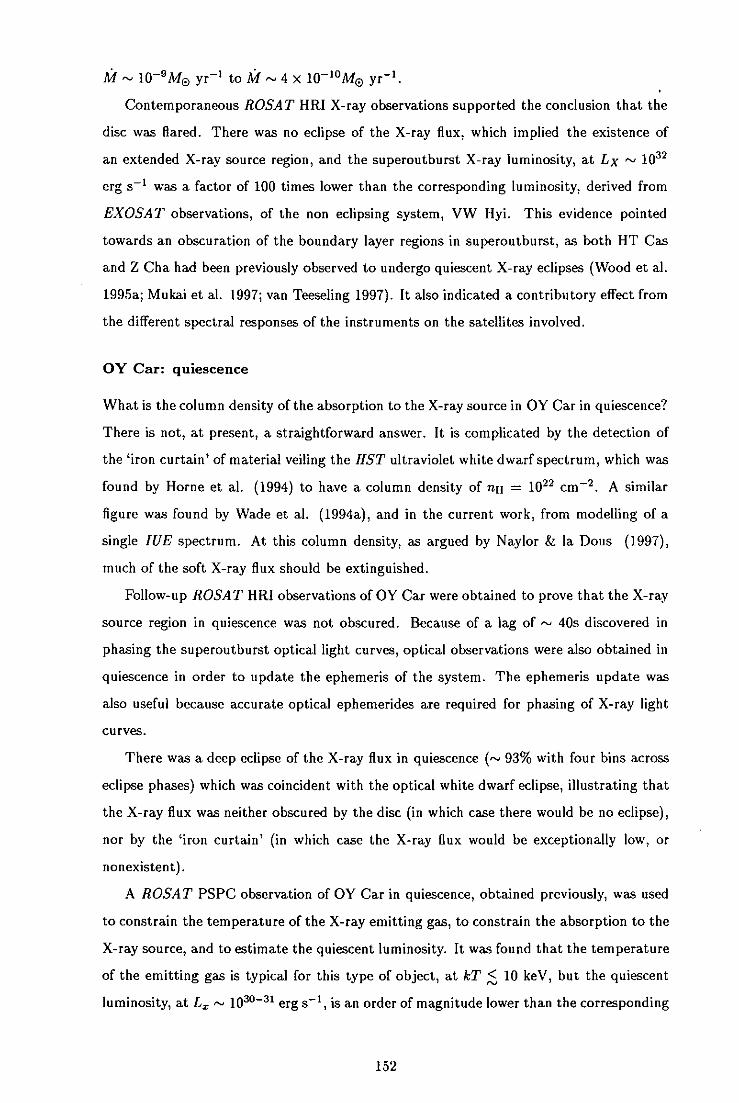
M 10 9 M® yr' to M'S-' 4 x 10'° M® yr.
Contemporaneous ROSAT HRI X-ray observations supported the conclusion that the
disc was flared. There was no eclipse of the X-ray flux, which implied the existence of
an extended X-ray source region, and the superoutburst X-ray luminosity, at Lx 1032
erg s was a factor of 100 times lower than the corresponding luminosity, derived from
EXOSAT observations, of the non eclipsing system, VW Hyi. This evidence pointed
towards an obscuration of the boundary layer regions in superoutburst, as both HT Cas
and Z Cha had been previously observed to undergo quiescent X-ray eclipses (Wood et al.
1995a; Mukai et al. 1997; van Teeseling 1997). It also indicated a contributory effect from
the different spectral responses of the instruments on the satellites involved.
OY Car: quiescence
What is the column density of the absorption to the X-ray source in OY Car in quiescence?
There is not, at present, a straightforward answer. It is complicated by the detection of
the 'iron curtain' of material veiling the HST ultraviolet white dwarf spectrum, which was
found by Home et al. (1994) to have a column density of nH = 1022 cm 2 . A similar
figure was found by Wade et al. (1994a), and in the current work, from modelling of a
single JUE spectrum. At this column density, as argued by Naylor & Ia Dolls (1997),
much of the soft X-ray flux should be extinguished.
Follow-up ROSAT HRI observations of OY Car were obtained to prove that the X-ray
source region in quiescence was not obscured. Because of a lag of r 40s discovered in
phasing the superoutburst optical light curves, optical observations were also obtained in
quiescence in order to update the ephemeris of the system. The ephemeris update was
also useful because accurate optical ephemerides are required for phasing of X-ray light
curves.
There was a deep eclipse of the X-ray flux in quiescence (r 93% with four bins across
eclipse phases) which was coincident with the optical white dwarf eclipse, illustrating that
the X-ray flux was neither obscured by the disc (in which case there would be no eclipse),
nor by the 'iron curtain' (in which case the X-ray flux would be exceptionally low, or
nonexistent).
A ROSAT PSPC observation of OY Car in quiescence, obtained previously, was used
to constrain the temperature of the X-ray emitting gas, to constrain the absorption to the
X-ray source, and to estimate the quiescent luminosity. It was found that the temperature
of the emitting gas is typical for this type of object, at kT < 10 keV, but the quiescent
luminosity, at L. '-' 1030_31 erg s, is an order of magnitude lower than the corresponding
152

luminosity of VW Hyi as measured by the same satellite. Two alternative explanations
are possible without invoking the absorption to the X-ray source - the white dwarf may
be spinning rapidly, or there may be a low rate of mass transfer through the boundary
layer.
The 1.6 kilosec observation, frustratingly, did not allow a quantitative estimate to
be made of the absorption due to interstellar hydrogen and locally to the 'iron curtain'.
Single component absorption models were not compatible with the column density of 10 22
cm 2 derived by Home et al. (1994). Model fits using a dual-component absorption could
not realistically disentangle the relative contributions of a local, ionized absorber and an
interstellar neutral absorber.
Tentatively, evidence presented here does seem to point to some contribution from
ionized material, reducing the X-ray opacity and allowing the detection of soft X-rays.
This is the first time a warm absorber has been invoked in the context of X-ray observations
of C Vs.
Archive ultraviolet observations
In most cases the ultraviolet light from the system is dominated by the accretion disc, but
in some cases the characteristic spectroscopic signature of a white dwarf can be detected
and modelled. This modelling allows the parameterisation of several attributes of the
white dwarf primary star.
As the largest archive store of ultraviolet observations, the IUEFA contains thousands
of CV spectra. In actual fact, the white dwarf can be observed in only a very small
number of these spectra. White dwarf model atmospheres and synthetic spectra were
generated, and those IUE CV spectra where the white dwarf could be seen were fitted
using a fitting routine based on the x2 value of the fit; this resulted in white dwarf
temperatures in good agreement with published values. In the case of CU Vel and SW
UMa, the derived temperatures agreed very well with (the same within the errors: +1500
K) those of Gänsicke & Koester (1999), who used the Kiel model atmosphere code.
In most of the above cases, the JUE spectrum can be modelled as a single white dwarf,
but the higher quality of HST and HUT spectra allow dual temperature models to be
fitted (Long et al. 1993), or allow the modelling of, for instance, accretion belts (Huang et
al. 1996). Outburst-quiescent datasets show that a substantial proportion of the decline
in the ultraviolet flux after outburst can be attributed to a cooling white dwarf (e.g.,
Gänsicke & Beuermann 1996).
An investigation of the accepted methods used to generate the model atmospheres and
153

synthetic spectra has suggested that derived white dwarf temperatures in CVs are subject
to some systematic uncertainties in the derived temperatures. This does not affect relative
temperature determinations, where the simple change in temperature is measured. The
two main causes of error are the neglect of metal line blanketing, which is acknowledged in
Home et al. (1994) to be an important effect, and the general assumption that the model
atmospheres will have a gravity logy = 8 (Mmd OMM® ). This is rather low compared to
estimates of the white dwarf mass in OY Car itself, based on eclipse durations (between
0.68 and 0.89M®). NLTE effects are negligible at the temperatures and gravities typical
of white dwarfs in dwarf novae.
6.2 Further work
6.2.1 Forthcoming observations with ASCA and the HST
Introduction
Early on in the course of this work, it was realised that the quality of the quiescent X-ray
spectrum of OY Car was sufficient only to weakly constrain the extent of the column
density of the absorption to the X-ray source. It was also recognised that potentially
serious discrepancies could develop between measurements of the column density in the
ultraviolet and those obtained in the X-ray (Naylor & Ia Dous 1997), and that these
potential discrepancies might be exacerbated by comparing observations obtained at dif-
ferent epochs. Simultaneous ultraviolet/X-ray observations in quiescence were needed to
specify the extent of the absorption in each spectral region.
A programme to observe OY Car simultaneously with ASCA and the HST was thus
drawn up for, respectively, ASCA AO-7 and HST Cycle 8. The proposals were drawn up
by the author and Dr. B.J.M. Hassall, in collaboration with Drs. J.H. Wood and K. Mukai,
and Prof. T. Naylor; the present author was a major contributor to the scientific cases
for both of these proposals. Each proposal was accepted after review by the respective
Time Allocation Committees, (60 kilosec and 2 orbits, respectively) and the observations
are scheduled to be acquired in 2000 Mar, unfortunately not in time for inclusion in this
thesis.
The reduction and analysis methods undertaken during the course of this thesis are
an excellent preparation for the forthcoming observations.
154

A SCA
With its increased throughput and spectral energy resolution, ASCA (Tanaka et al. 1994)
observations will be a significant improvement over those already acquired with ROSAT.
The mean count rate of the ROSAT PSPC observation detailed in Chapter 4 was 0.08
counts s (note however that the count rate in the PSPC all-sky survey was 0.024 counts
r'). PIMMS (Mukai 1993) predicts an ASCA count rate of 0.15 - 0.2 counts C 1 per
instrument, assuming the PSPC count rate above and a 2 - 10 keV bremsstrahlung model
absorbed with NH = 1022 cm 2 . This should be compared with -.' 0.12 counts C' for the
HT Cas observation by Mukai et al. (1997).
Were it not for noise contributions from the background, the 60 kilosec observation
would yield a folded light curve of the quality of that obtained by Mukai et al. (1997).
That said, with the ASCA count rate estimated above, and assuming enough eclipses
are covered, it may be possible to measure the eclipse width and depth accurately. The
summed ASCA eclipse can be used to compare X-ray and optical eclipse timings, and in
principle the phase duration of the X-ray ingress and egress can be compared with those
in the optical. The feasibility of this is illustrated by Mukai et al. (1997), who model the
ASCA X-ray eclipse of HT Cas to put real limits on the size of the X-ray emitting region,
and the location of the emission relative to the white dwarf.
The observational aspect that is expected to bear the most scientific fruit, however,
is the X-ray spectrum. The ASCA X-ray instruments have a wider passband (0.4 - 10
key) and finer energy resolution than those on ROSAT, which will result in a substantial
refinement of the X-ray spectrum of OY Car. A summed spectrum obtained over 60 kilosec
will enable concrete constraints to be placed on the absorption to the X-ray source. Dual-
component absorption models will be used to estimate the relative contributions of the
local absorption due to the 'iron curtain' and the neutral interstellar absorption. This will
then be compared to the absorption deduced from the HST ultraviolet observations. A
boundary layer X-ray luminosity and accretion rate will also be estimated. In the absence
of an X-ray eclipse (highly unlikely), modelling of the highly absorbed boundary layer
component will be undertaken.
Finally, the occurrence of absorption dips in the X-ray light curve, at other orbital
phases away from eclipse, will be investigated. This will probe the phase dependence
of any absorption variation, and if detected will imply azimuthal variation of extended
structure in the outer disc. If such dips are present at 0 ".' 0.7— 0.8, it is likely that they
will be due to the bright spot. If there are dips at other orbital phases, these should be
155

detectable by comparing hard (E > 2 key) and soft (E < 2 key) light curves.
HST
The simultaneous observations from the HST will enable well-defined constraints to be
placed on the absorption in OY Car in the ultraviolet spectral range. Initially, this obser-
vation will help assess the effect of time variability as a cause of the discrepancy between
the measured column densities in each spectral range.
OY Car will be observed with the STIS, using the CCD detectors rather than the
MAMA (Multi-Anode Microchannel Array), which would be vulnerable if the system
undergoes an outburst in mid-observation. The G230LB grating will be used to cover a
wavelength range of 1685 - 3065 A, with a central wavelength of 2375A. Signal to noise is
expected to be r.., 10 per resolution element for a five minute exposure. The white dwarf
spectrum should be relatively flat and featureless over this spectral region, whilst the
'iron curtain' has many individual lines and a large depression between 2000 and 3000A,
which should amount to over 50% percent of the flux at the column densities expected.
Figure 6.1 illustrates the predicted effect of the 'iron curtain' on the flux in the wavelength
range of the forthcoming observations. The by a region will be absent as the forthcoming
observations do not cover that wavelength; however, the slope of the continuum will be
a sufficient diagnostic of the temperature. Meanwhile, the 'iron curtain' effects are more
pronounced at "-' 2500A than at r 1600A, which will enable better constraints to be placed
on the column density and other parameters than has been possible thus far.
The author is under no illusions that the HST spectrum of OY Car will require careful
reduction and analysis. Contributions to the spectrum from the residual disc and bright
spot emission will have to be removed so that the spectrum that is eventually modelled is
that of the veiled white dwarf only. Judging from the 1150 - 2500A spectrum obtained by
Home et al. (1994), the combined disc/bright spot contribution will begin to be noticeable
longward of r'.' 2200A. The method envisaged for spectrum decomposition will be similar
to that developed in Home et al. (1994) and in the HST observations of UX UMa and
V2051 Oph by Baptista et al. (1998a, b). In order to do this, the spectra will have to
be binned and flux-calibrated, to give spectrophotometric light curves. This will involve
dividing the spectra into short (15-30A) passbands and computing the average flux in
each. From these light curves, the system can be modelled and the spectra decomposed
into each contributory element.
The light curves reconstructed from the spectra will then be decomposed into white
dwarf, bright spot and accretion disc components in a similar fashion to that described
156

0
x N
0
0,
1; an
1800 2000 2200 2400 2600 2800 3000
Wavelength (A)
Figure 6.1: Synthetic spectra of a solar composition white dwarf with Tff = 16,500 K (grey), and the
same spectrum obscured with a solar abundance LTE veiling gas with T5 = 10,000 K, = 1022 cm 2
(black). The wavelength range and resolution is identical to that of the forthcoming HST observations.
While the Ly a absorption is not covered, the continuum slope should provide a sufficient diagnostic for
the white dwarf temperature.
157

as follows, using a variation of the method of Wood et al. (1985): in this way the data
D(Ø, A) are acquired. In Home et al. (1994), the data D(, A) are modelled as M(Ø, A)
given by the sum of several components:
(6.1)
where L1() is the light curve and S1(A) is the spectrum of component i. Each data
component light curve (white dwarf, bright spot, and accretion disc) can be modelled
by imposing model light curve constraints such as assuming that the white dwarf and
accretion disc light curves be symmetric about phase 0. Also, since the white dwarf and
bright spot are totally eclipsed in OY Car, these model component light curves must have
a flux of zero between second and third contact points. The component light curves and
spectra can then be adjusted as parameters in the model M(, A) in order to achieve the
best fit to the data D(, A), using the x2 statistic. The corresponding spectra will be
reconstructed from a linear combination fit of the three model component light curves to
the data.
Once the veiled white dwarf spectrum is extracted, it will be modelled with synthetic
spectra generated using TLUSTY and SYNSPEC. Fully line blanketed models can be
used, as the temperature of the white dwarf should at this stage be known to within
a few thousand degrees. Optimised model parameters will be calculated using the im-
proved methods outlined in Section 5.8, i.e., using the multidimensional downhill simplex
AMOEBA algorithm from Press et al. (1992). However, optimisation using this method
requires vigilance as the algorithm sometimes lodges in a local minimum.
An alternative approach to optimising model parameters would be to use an evolution-
ary strategy (genetic) algorithm (GA). Although GAs cannot be guaranteed to find the
global local minimum, they do have the advantage of being able to climb "uphill" to some
extent, which is a feature downhill simplex and similar methods lack. GAs work along the
following lines:
1. Generate a set of random solutions to the problem.
2. Evaluate the solutions, minimise according to an appropriate statistic (e.g., x2 ) and
rank accordingly.
3. Generate the next generation of solutions. "Natural selection" is used here in GAs,
meaning that the fittest solutions (i.e. the ones ranked best in terms of the mm-
imising function) are more likely to produce offspring than those ranked lower. In
practice, this is achieved by assigning a success probability to each of the solutions
158

in the previous population. Then pairs of solutions to mate are picked, according to
their probability of success, to produce offspring. To produce the offspring, so-called
"uniform crossover" (Beasley et al. 1993b) is used, which means that each parameter
of the offspring solution is taken from either one or the other parent solution.
GAs have been introduced into astrophysics only recently. For reviews of the method,
see Beasley et al. (1993a, b). Example applications of GAs to the mapping of the accretion
stream and in finding the geometry of the accretion region in polar CVs can be found in
Hakala (1995) and Potter et al. (1998).
It is envisaged that a method similar to that used for field white dwarfs by Finley et al.
(1997) will be used to calculate very accurate values for several parameters, including the
temperature and gravity, in OY Car. Once the x2 is calculated for each model, Finley et
al. (1997) find the best fitting values for the Teff and log g by fitting bicubic polynomials
to each x2 surface in the region of the minimum x2 Finley et al. (1997) then find hi and
2a limits on the derived Teff and log g by polynomial interpolation of the x2 array onto a
denser Tff - logg grid. This method can potentially be applied to other parameters such
as the column density etc.
In this way, accurate values for not only the ultraviolet column density, but also the
white dwarf temperature and gravity, electron density of the veiling curtain, veiling curtain
temperature and veiling curtain velocity dispersion will be derived, simultaneously with X-
ray spectral temperature, column density and eclipse parameters. The use of improved and
more accurate model atmospheres and synthetic spectra will enable further constraints to
be placed on system parameters in the ultraviolet, while the greater spectral and temporal
resolution of ASGA will improve our knowledge of the system in the X-ray.
6.2.2 Future observations
A new generation of X-ray satellites with ever-higher sensitivity and capabilities will soon
be available. The main two are Chandra, a NASA satellite launched successfully on 1999
July 23, and an ESA Cornerstone project, the X-ray Multi-mirror Mission (XMM), which
at the time of writing is scheduled for launch 1999 mid-December. As XMM is an ESA
mission, the lion's share of the observing time is set aside for European astronomers.
This Section will concentrate on how the increased capability of XMM can be used to
investigate some of the still outstanding questions regarding CVs in outburst or high mass
accretion rate systems.
XMM carries three grazing incidence Wolter type-i X-ray telescopes which have a
total effective area of 4650 cm 2 at lkeV, approximately 6 times that of Chandro and 12
159

times that of ROSAT. XMM science instruments are:
• The European Photon Imaging Camera (EPIC), consisting of 3 CCD cameras for
X-ray imaging, moderate resolution spectroscopy (E/zlE 20 - 50) and X-ray
photometry. XMM carries two different types of EPIC cameras. Two of the X-ray
telescopes are equipped with an EPIC MOS (Metal Oxide Semiconductor) and the
third focuses onto an EPIC pn. The main differences between the cameras are that
the MOS CCD is front-illuminated while the pn camera is back-illuminated, and a
considerably faster readout time for the pn chips.
• The Reflection Grating Spectrometer (RGS), fitted to two of the X-ray telescopes,
consisting of two essentially identical spectrometers for high-resolution spectroscopy
and spectrophotometry (E/AE - 200 - 800), operable in either spectroscopy or
high-time resolution modes.
• The Optical Monitor (OM): XMM is unique in being equipped with an additional
co-aligned 30cm optical/UV telescope, the OM, providing for the first time the
opportunity to observe simultaneously across optical/UV and X-ray wavelengths.
The total bandwidth of the OM is 1600-6000 A, and its detector is operated as a
photon-counting instrument. The OM is more sensitive than a ground-based tele-
scope of equivalent aperture because of the lack of atmospheric extinction. The
OM is equipped with a filter wheel containing several filters (U, B, V, white), and
two grisms covering different wavelength ranges and capable of moderate resolution
optical/UV spectroscopy (r.s 5 A in the UV).
All six science instruments are operated simultaneously, and each instrument can be
operated independently in different data acquisition modes.
Enduring questions concerning CVs in the high mass accretion rate regime, may be
answered by further X-ray and ultraviolet observations. The author, in collaboration with
Drs. B.J.M. Hassall, J.H. Wood, K. Mukai, and Prof. T. Naylor, has submitted two
proposals for observing time on XMM (AO-1). The intention was to observe the X-ray
brightest eclipsing novalike variable, UX UMa, and our old friend OY Car in superoutburst,
in complementary proposals.
The UX UMa proposal, for which the present author is P1, has recently (1999 Dec)
been allocated the requested 51 kilosec of observing time (the OY Car proposal, which was
TOO, was unfortunately not allocated time). 51 kilosec is approximately 3 orbital periods
of UX UMa. The orbit of XMM is highly elliptical, and in principle allows continuous
target visibility of up to 70 kilosec. Thus UX UMa will be observed continuously for an
160

unprecedented length of time for an X-ray observation, allowing any variability of the X-
ray flux to be investigated. Other questions which may be answered by these observations
include
• What is the source of the X-ray emission in the high mass accretion rate
regime?: In Chapter 3, Section 3.6.1, there is a discussion of the different X-ray
spectral components observed in the spectrum of VW Hyi in outburst and super-
outburst. To recap briefly, the X-ray emitting region of VW Hyi and some other
non-eclipsing systems in outburst (and superoutburst) display a two-component X-
ray spectrum. The optically thick blackbody-like component at kT r'., 10 - 50 eV
originates from the boundary layer and dominates up to r 0.5 key. The hard, opti-
cally thin component is modelled with a 5- 10 key thermal bremsstrahlung spectrum
and can be detected down to r'. 0.1 key if the absorption is low. However the source
of the latter component is still unknown. If the component is residual optically thin
emission from the boundary layer, as suggested by the EXOSAT observations of VW
Hyi (van Teeseling et al. 1993), then this component will undergo an eclipse in a
high inclination system. This has not been the case with OY Car in superoutburst
(Naylor et al. 1988; and this work), and may be due to a considerable contribu-
tion of the blackbody component to the flux detected in each satellite filter. The
vastly increased sensitivity of XMM should enable the separate detection of the hard
component, and in principle enable constraints to be placed on it.
• Is the extended X-ray source in outburst a wind or a static corona?: The
timing observations of lix UMa and OY Car in superoutburst make it clear by the
lack of eclipse that extended regions produce the UV emission lines (the wind) and
the X-rays. However, it is still unclear whether the sources of each emission are
coincident. For example, it is perfectly possible that the hard X-rays have their
origin in a static, hot, optically thin corona rather than in an outflow such as a wind
(Naylor & Ia Dous 1997). The high time resolution RGS spectrum will provide an
answer to this question, because a static coronal X-ray source will produce narrow
emission lines (FWHM r.s 300 km s') while an X-ray source originating in a wind
will produce broad emission lines (FWHM is.' 1500 km s'). Figure 6.2 simulates the
expected appearance of the 0 VIII emission line at 0.65 keV when the source is (a)
a static corona and (b) a wind.
• What is the extent of the 'iron curtain'/absorption in outburst?: The 'iron
curtain' appears in quiescence and contributes to the opacity (and hence absorption)
161

osi- I .....I I-. I I -.1
UK'
0.2
UNU] 0.54 0.55 0.54 0.55
Figure 6.2: Left: A simulated RGS spectrum representing an X-ray source that is a static corona,
producing a narrow emission line. Right: If the source of the X-ray emission in superoutburst is the wind,
then the emission line will be broad. The thfference between the two can clearly be seen. The FWHM of
the narrow simulation is 325 km s, while the width of the broad simulation (FWHM 1500 km s')
can be determined to about 30% accuracy. Simulation by Dr. K. Mukai (private comm.).
in the ultraviolet and the X-ray. But there are no measurements of the extent of the
X-ray column in outburst. Any investigation of this particular aspect should also
have simultaneous ultraviolet coverage to measure and search for variations, orbital
or otherwise, in the ultraviolet column.
With XMM, absolutely simultaneous coverage in the optical/UV and X-ray is pos-
sible, removing the need to use two different satellites such as those observations
detailed in Section 6.2.1. The XMM OM spectral resolution is sufficient to resolve
the broad depression at A 2500A, and again, the increased spectral and temporal
resolution will allow further constraints, over and above those available from ROSAT
and ASGA, to be placed on the absorption to the X-ray source.
• What fraction of the X-ray flux, if any, comes from the secondary star?:
As pointed out in the Introduction, the corona of the secondary star is potentially a
source of X-rays. Like in the quiescent case, timing observations of eclipsing systems
are the most useful method for detecting physical components. The disc will eclipse
the secondary star, producing a drop in the X-rays at orbital phase 0.5 which is
in principle detectable. An observation of this kind would show for the first time
whether or not the secondary star is a significant contributor to the X-ray flux from
CVs.
Figure 6.3 shows a simulated eclipse of the secondary star by the accretion disc in
162
1.0 1.2 1.4 1.6 1.8 2.0 ORBITAL PEASE
Figure 6.3: A simulation of an eclipse of the X-ray emitting secondary star by the accretion disc in UX
UMa (feature at phase 0.5) as observed by XMM (predicted). This is a best case scenario, assuming that
all X-rays come from the secondary star. Simulation by Prof. T. Naylor (private comm.).
UX UMa, obtained from the total count expected from all three XMM detectors,
folded on orbital phase. The total exposure time corresponds to 3 orbital cycles
(51ks). The parameters assumed are the best available for UX UMa, and include
a disc with a semi-opening angle of 100. For this simulation it is assumed that the
secondary star is the only source of the X-rays. This eclipse is significant at the
9c-level. If, say, only a third of the X-rays had an origin on the secondary star, the
eclipse would be significant at the 3a-level.
Endpiece
The observations presented here have provided further insights into the characterisation of
the components, both physical and spectral, in CVs. Further, multiwavelength, preferably
simultaneous, observations are necessary. These will test whether the conclusions of this
thesis can hold up in the face of the greater and greater spectral/temporal resolution
available from the next generation of satellites and telescopes. Only by observing CVs in
the entire range of their emissions can a self-consistent picture of their behaviour be built
up. As the quality of our observations improve, so too does our understanding of these
intriguing systems.
163

Appendix A
The Zanstra method applied to
CV winds
The Zanstra method has been used for many years as a way of determining the temperature
of the exciting stars in nebular astrophysics. It is fully described in Osterbrook (1989); this
is the version used by Hoare and Drew (1991) to estimate CV boundary layer temperatures.
If the CV wind is optically thick in the He II Lyman continuum, it will absorb all the
ionizing photons. Thus the total number of ionizations is equal to the total number of
ionizing photons emitted. Ionization equilibrium requires that:
too F I l-'w
du fntitneas(HetT)dv ( A.1) —= 1w
number of photoionizations = number of recombinations,
where L is the energy distribution of the ionizing source, v0 = 54.4 eV is the frequency
corresponding to the ionization potential of He II, and aB is the recombination coefficient.
The ionizing source is the accretion disc plus boundary layer.
The number of recombinations can be measured by observing an He II recombination
line such as A1640 or .X4686. Hoare & Drew (1991) follow Bohlin et al. (1982) and express
the ratios in fluxes, obtaining
[ dv = 1.56 x 10 11 f(A1640) (A.2) i 0 1w
and
[= 9.8 x 10 11 J(A4686) (A.3) iwo hi.'
assuming that Te in the wind is 10 1 K. Hoare & Drew (1991) state that if the wind
temperature was as high as 50,000 K the values would increase by only 20 percent and 60
percent, respectively.
164

The Zanstra ratio is defined as
COO
G(A228, A.) = "° f/hvdu
1.1h (A.4)
where .1. is the continuum flux of the ionizing source at wavelength A., which has been
chosen to be next to the recombination line question to avoid the effects of reddening.
The Zanstra ratio gives the ratio of the number of photons with E > 54.4 eV to the
ultraviolet/optical flux.
Foreshortening effects due to the inclination of the disc relative to the observer's line of
sight are corrected by dividing the continuum flux by cos i. Hoare & Drew (1991) comment
that another effect of the disc geometry is that approximately half the recombination line
photons will be intercepted by the disc and destroyed, and therefore they multiply the
observed recombination line flux by a factor of two.
Hoare & Drew (1991) then combined equations A.2, A.3 and A.4 to express the Zanstra
ratio in terms of observable quantities:
G(A228, 1800A) = 2.4 x 10³ J(A1640)
(A.5) f.(1800A)
and
G(A228,4700A) = 1.3 x 10³ f(A4686)
(A.6) f, @ 700AY
The quantity f(line) is the observed recombination line flux (ergs cm 2 s) and f. is the
observed continuum flux/cosi in ergs cm 2 s A_I). Backscattering losses are included
in the numerical constant.
Hoare & Drew calculated a theoretical spectrum for the ionizing continuum from a
two component model consisting of a steady state accretion disc (calculated by either
integrating blackbodies or Kurucz model atmospheres at approproate temperatures over
the disc), and a boundary layer component represented by a blackbody, an NLTE model
atmosphere, or a Raymond-Smith plasma model.
165

Appendix B
Overview of the basic equations
used in model stellar atmosphere
generation
The reader is referred to Mihalas (1978), Gray (1992) or Werner & Dreizler (1999) for
a discussion of this subject from first principles, and a review of the CL/ALl method of
solution. As discussed in Section 5.6, a typical model atmosphere generation program
simultaneously solves the 5 basic equations, namely: radiative transfer, hydrostatic equi-
librium, radiative equilibrium, particle conservation and statistical equilibrium.
Definitions
Consider radiation coming from a small portion, area AA, of a surface. The specific
intensity of the radiation is defined as:
= lim cos OAA&thtzXv Un
- dE,.
- cos9dAdwdtdv (B.2)
where the limit is taken as all quantities, áÂ, &a the increment of solid angle, At the
increment of time, and zv the spectral band, diminish towards zero. The units of specific
intensity can be I,. or 'A, where the relation between these quantities is:
= IxdA.
The mean intensity, Jr,, is defined as the directional average of the specific intensity,
and is related to the energy density of the radiation field, where:
= JIudw. (B.4)
166

.1,, is sometimes referred to as the zeroth moment of the specific intensity. The first
moment, H,,, is related to the flux, where:
H,, = - ft cos 0 dw, (B.5)
while the second moment, K,.., is related to the radiation pressure and is used in the
hydrostatic equation:
K,, = _ fI, icos2 9dw. (B.6)
The flux is the measure of the net energy flow across the area z\A in time zt, in spectral
range at-., as these quantities approach the limit:
F - fdE,, - dAdtdt/
(B.7)
The flux and specific intensity can then be related using eq. B.2 to get:
P,1 = flv cosedw. (B.8)
and, following similar arguments,
F,, = 47rH,, (B.9)
Two physical processes contribute to the absorption coefficient, ic,,. The first is true
absorption where the photon is absorbed and the energy thermalized (bound-free), the
second is scattering, where the photon is scattered out of the solid angle being considered
(free-free). The amount by which the specific intensity is diminished in a length dx is:
dl,, = —.'çpldx, (B.1O)
where p is the density in mass per unit volume. K,, has units of area per unit mass. Most
of the absorption comes from hydrogen in one form or other.
The optical depth r,, can now be defined over the path length L as:
pL
TV = J ,c,,pdx. (B.11)
0
Eq. B.10 can now be rewritten as:
dl,, = —I,.,dr,,. (B.12)
This simple form of the radiative transfer equation can be solved to reveal the extinction
law:
I,, = I,, ° exp(—r,4. (B.13)
167

The emisson coefficient j,, is a measure of the the amount of radiation emitted. In an
analagous fashion to the case for absorption, the two contributing factors to the emission
coefficient are emission itself and scattering of photons into the line of sight. The increase
in the specific intensity in a length dx due to emission is:
dJ,, = j,,pdx. (B.14)
We finally come to the definition of the source function, defined as the ratio of emission
to absorption:
SV =
(Bd5)
The source function has the same units as the specific intensity. In [ATE, S. =
where B,, is the blackbody function and T is the temperature.
Radiative transfer equation
If we consider radiation travelling in a direction it, the change in the specific intensity, dI,,,
over a small element of path length du, is the sum of the losses and gains from emission
and absorption:
(B.16) dI,, = —n,,pI,,dn + j,,pdu.
Dividing across by icpdu (eq. B.11), and using eq. B.15, this reduces to:
dI,,/dr,, = —1,, + S.
This is a basic form of the radiative transfer equation.
TLUSTY uses a radiative transfer equation written as
pOJ(z, p, ii) = —ic(z, u)I(z, p, v) + j(z, ii),
(B.17)
(B.18)
where z is the geometrical depth, p is the cosine of the angle between the direction of prop-
agation and the normal to the surface, i' is the frequency, and I, ic and j have their usual
meanings. The transfer equation is considered by TLUSTY in two different forms - the
full angle-dependent form, and the Eddington-factor form, used for linearization. Further
details of these treatments, including the variables introduced and boundary conditions
used, can be found in Hubeny (1988).

The hydrostatic equilibrium equation
TLJUSTY uses a generalisation of the hydrostatic equation:
dP/dm = g, (B.19)
where P is the pressure, m is the mass and g is the gravity. Now,
P=Pgas+Prad+Pturb. (B.20)
In TLUSTY, these contributions to the pressure are defined by:
Pgas = nkT (B.21)
Prad = - [ K,..dv (B.22) ci
Pturh = ( 1/2)PV urb (B.23)
where these are the gas, radiative and turbulent pressures respectively, and the K-integral,
K, is defined in eq. B.6. Here, ii is the particle number density and k is the Boltzmann
constant.
The radiative equilibrium equation
The radiative equilibrium equation arises from the application of conservation of energy
to the flow of energy upward through the stellar photosphere. TLUSTY uses two dif-
ferent forms of the radiative equilibrium equation, one an integral equation, the other a
differential equation. The standard integral form is:
- S)du = 0, (B.24)
while the differential form is:
f°°d 4 —dv - (B.25)
K
dr 4ir
Hubeny (1988) finds that the differential form is more accurate at large depths, while the
integral form is preferable for small depths.
The statistical equilibrium equations
The equations of statistical equilibrium (or rate equations) are used to calculate the actual
occupation numbers of the bound and free states of atoms in stellar atmospheres. The
general form is derived in Mihalas (1978), p 127, and the application of these equations
to model stellar atmosphere generation can be found in Mihalas (1978) p 137-145, and
Hubeny (1988).
169

Application in TLUSTY
The reader is referred to Hubeny (1988) for a complete description of TLUSTY, from
which this précis is derived, and also to Section 5.6.1. TLIJSTY computes model stellar
atmospheres assuming a plane-parallel, horizontally homogeneous atmosphere in radiative
and hydrostatic equilibrium. It allows for departures from LTE for a set of occupation
numbers of selected atomic and ionic energy levels.
The set of equations comprising radiative transfer, hydrostatic equilibrium, raditive
equilibrium and statistical equilibrium is highly coupled and non-linear. TLUSTY solves
this set of equations using the complete linearization technique pioneered by Aeur &
Mihalas (1969), which in essence involves the discretization of the equation set by depth
and frequency. This allows iterative solutions to be found by the use of a different set of
linear equations for corrections to the values of all quantities from the previous interation.
With TLUSTY, computer time is saved by the introduction of so-called fixed-option
atomic transitions, which are treated exactly but are not linearized. The program of-
fers several options to avert divergences. Additionally, the program can allow options
which accelerate convergence of the complete linearization iterations, based on a set of the
equivalent two-level-atom procedures for selected atomic transitions performed between
two conseutive iterations.
The synthetic spectrum
The calculation of the synthetic spectrum from the model atmosphere is achieved by
expanding the flux integral (eq. B.7) in spherical polar coordinates and assuming no az-
imuthal dependence in 4.. The emergent flux in a line at frequency ii be calculated using:
F = 27r SE2(r tc ) rodlog r. (8.26)
ic0 loge
Here, the surface flux is the sum of the source function (8,..) at each depth multiplied
by an extinction factor, E2, appropriate to that depth; the integral is evaluated over all
appropriate depths. The optical depth scales are related by
dx = dr/tcp = dro/icop
where pc,, is the mass absorption coefficient, r, is the optical depth, and ,ç0 and 7-0 are the
same quantities at some reference wavelength used in the iteration of the spectrum. In
LTE, S(ro ) = B[T(ro)].
170

Appendix C
Details of TLUSTY and
SYNSPEC input and output files
All input and output files are in ASCII format.
TLUSTY195
S Input files:
- Unit 5: Main control data. This file contains the values of Teff and log g,
the LTE/LTGRAY switch, the name of the file that details the non-standard
parameters (of which there are about 90, ranging from auxiliary physical para-
maters to flags for selecting the treatment of the statistical equilibrium equa-
tion), the number of frequency points to read (these describe the continua),
the filenames of the explicit ions used in the calculation of the opacities, the
filenames containing the data for the explicit ions (including all energy levels,
bound-free transitions and bou nd-bound transitions);
- Unit 8: Starting model atmosphere. This is not needed if the model being
calculated is the initial LTE model atmosphere - in this case the input model
atmosphere is assumed grey (i.e. ,c is independent of ii).
A sample Unit 5 input file for a simple LTE model atmosphere with Teff = 35,000
K, logg = 4, composed of H and He only, is shown below:
35000. 4.0 ! TEFF, GRA/
T T ! LTE, LTGRAY
no change of general non-standard parameters
171

* frequencies
50 NFREAD
* data for atoms
*
2 NATOMS
* mode abn modpf
2 0 0
2 0 0
* data for ions
*
*iat iz nlevs ilast ilvlin nonstd typion fuel
*
1 0 9 0 100 0 ' H 1' 'hl.dat'
1 1 1 1 0 0 'H2'''
2 0 14 0 100 0 'He 1' 'hel.dat'
2 1 14 0 100 0 'He 2' 'he2.dat'
2 2 1 1 0 0 'He 3'
0 0 0 -1 0 0
*
* end
Output files:
- Unit 6: Standard output. This is a general log of the model construction
procedure in which tab!es display input data and performance messages;
- Unit 7: Condensed, machine-readab!e model atmosphere, for use as the input
to another run of TLUSTY or for use as the input Unit 8 with SYNSPEC;
- Unit 9: Convergence !og. This file is very important because it contains the
information on whether the model converged or not;
- Unit 10: Performance and error !og.
172

SYNSPEC42
SYNSPEC42 has five basic modes of operation, controlled by the switch IMODE. These
modes are (Hubeny & Lanz 1997):
. DIODE = 0: Normal synthetic spectrum (identification table and emergent flux);
. DIODE = 1: Detailed profiles of a few individual lines;
IMODE = 2: Emergent flux in the continuum + hydrogen and helium lines;
. IMODE = -1: Line identification table only - a list of lines which contribute to the
opacity at a given wavelength;
• IMODE = -2: The "iron curtain" option, detailed in Section 5.6.2.
The IMODE switch is located in Unit 55.
S Input files:
- Unit 5: Same main control data used for TLUSTY;
- Unit 55: Basic parameters for the synthetic spectrum including the LTE/NLTE
switch, the standard depth parameter (the depth at which the continuum opti-
cal depth is of order unity), the start and end wavelengths of the spectrum, the
wavelength scale, a switch giving the name of the file containing new chemical
abundances if necessary, etc;
- Unit 8: Input mode atmosphere (TLUSTY Unit 7);
- Unit 19: The line list, which in the JUE spectral range contains about 185 000
lines.
- Optional input files, of which there are 9, containing data for detailed line
profiles, changes in chemical composition etc.
A sample Unit 55 input file containing the basic parameters for a simple H/He only
synthetic spectrum in the wavelength range 1000 - 2200 A, is shown below:
2 46 0 IMODE, IDSTD, IPRIN
1 0 0 1 !INPUT MODEL (1=TLUSTY), INTRPL, ICHANGE, ICHEMC
IOPHLI
1 0 0 0 1 !IFREQ, INLTE, ICONTL, INLIST, IFHE2
0 0 0 !IHYRPR,IHEIPR, IHE2PR
173

1000 2200 5 10 1.d-4 0.1 !ALAMO,ALAST,CUTOFO,CUTOFFS,ItELOP,SPACING (A)
1. !VTB
10 0.1 1 NMU0, ANGO, IFLUX
. Output files
- Unit 6: Standard output, a general log of the procedure;
- Units 7 and 17: Emergent flux of the spectrum and theoretical continuum;
- Units 12 and 14: Line identification tables;
- Unit 16: Approximate equivalent widths of the lines;
- Optional Units 10 and 18: emergent specific intensities for the spectrum and
continuum.
On output from SYNSPEC42, the synthetic spectrum is ready for rotational and in-
strumental convolution using ROTIN4.
174

Appendix D
Acronyms used
AL! - accelerated lambda iteration
ASGA - Advanced Satellite for Cosmology and Astrophysics (formerly ASTRO-D)
BL - boundary layer
CL - complete linearization
CTIO - Cerro Tololo Inter-American Observatory (Chile)
CV - cataclysmic variable
DN - dwarf nova
EPIC - European Photon Imaging Camera (XMM instrument, of which there are two types with different sensitivity and readout characteristics: the EPIC MOS [Metal Oxide Semiconductor] and the EPIC pn)
EUVE - Extreme Ultraviolet Explorer
EXOSAT - European X-ray Observatory Satellite
FOS - Faint Object Spectrograph (HST instrument)
GSOC - German Science Operations Centre
HR! - High Resolution Imager (ROSAT instrument)
HST— Hubble Space Telescope
JUE - International Ultraviolet Explorer
LUEFA - IUE Final Archive
LEDAS - Leicester Database and Archive Service
LMXB - Low Mass X-ray Binary
MAMA - Multi-Anode Microchannel Array (HST instrument)
MCP - Microchannel Plate
MEM - Maximum Entropy Method
(N)LTE - (non-) Local Thermodynamic Equilibrium
175
NL - novalike variable
NMCV - non-magnetic cataclysmic variable
OM - Optical Monitor (XMM instrument)
PPEM - Physical Parameter Eclipse Mapping
RGS - Reflection Grating Spectrograph (XMM instrument)
ROSAT - Röntgen Satellite
SAAO - South African Astronomical Observatory
STIS - Space Telescope Imaging Spectrograph (HST instrument)
SUI - Spectrum Under the Influence (of an emitting or absorbing body)
TOAD - Tremendous Amplitude Outburst Dwarf nova, the WZ Sge subclass.
VSS RAS NZ - Variable Star Section of the Royal Astronomical Society of New Zealand
WD - white dwarf
WFC - Wide Field Camera (ROSAT instrument)
XMM - X-ray Multi-mirror Mission
XRT - the X-ray Telescope on ROSAT
176

References
Aeur LII., Mihalas D., 1969, ApJ, 158, 641.
Allan D.J., Valiance R.J., 1995, ASTEHJX - X-ray data processing system, STARLINK User Note
98.
Anderson L.S., 1989, Api, 339, 558.
Applegate, J.H., 1992, ApJ, 385, 621.
Arnaud K.A., 1996, in Astronomical Data Analysis Software and Systems V, eds. Jacoby G. and
Barnes i. ASP Conf. Series volume 101.
Baptista R., Steiner J.E., 1991, A&A, 249, 284.
Baptista R., Steiner i.E., 1993, A&A, 277, 331.
Baptista R., Home K., Wade R.A., Long KS., Rutten R.G.M., 1998, MNRAS, 298, 1079.
Baptista R., Catalan S., Home K., Zilli D., 1998, MNRAS, 300, 233
Barstow M.A., Fleming TA., Diamond Ci., Finley U.S., Sansom A.E., Rosen SR., Koester D.,
Holberg J.B., Marsh M.C., Kidder K., 1993, MNRAS, 264, 16
Bath G.T., 1969, Api, 158, 571.
Bath G.T., 1975, MNRAS, 171, 311.
Bath G.T., Evans W.D., Pringle i.E., 1974, MNRAS, 166, 113.
Beasley D., Bull DR., Martin R.R., 1993a, University Computing, 15(2), 58.
Beasley D., Bull DR., Martin R.R., 1993b, University Computing, 15(4), 170.
Belloni T., Verbunt F., Beuermann K., Bunk W., Izzo C., Kley W., Pietsch W., Ritter H., Thomas
H.C., Voges W., 1991, A&A, 246, L44.
Berriman G., 1987, MNRAS, 228, 729.
Billington I., Marsh T.R., Home K., Cheng F-H., Thomas G., Bruch A., O'Donoghue D., Eracleous
M., 1996, MNRAS, 279, 1274.
Breedon L., et al. (The VFOOLS Group) 1997, The User's Guide to FT00LS, High-Energy Astro-
physics and Space Research Centre, NASA-GSFC.
Briel U.G., Pfeffermann FL, 1995, SPIE (Soft X-ray Optics and Technology), 2518, 120.
Briel U.G., et at. 1996, ROSAT User's Handbook, Max-Planck-lnstitut für extraterrestrische
Physik, 85740 Garching, Germany.
Bryan R.K., Skilling J., 1980, MNB.AS, 191, 69.
Burch S.F., Gull S.F., Skilling i. 1983, Comp. Vis. Graph. Im. Proces., 23, 113.
Cannon C.J., 1973b, Api, 185, 621.
Catalán MS., Home K., Cheng F.-H., Marsh Ta., Hubeny 1., 1998, in ASP Conf. Ser. 137, Wild
Stars in the Old West, ads. S. Howell, E. Kuulkers, C. Woodward, ASP San Francisco.
Cheng F.-H., Sion EM., Home K., Hubeny I., Huang m., Vritelek S.D., 1997a, Ai, 114, 1165.
Cheng F.-H., Sion EM., Szkody P., Huang M., 1997b, Api, 484, L149.
Cook M.C., 1985, MNRAS, 215, 211.
Córdova F.A., Mason K.O., Api, 260, 716.
Córdova F.A., Mason K.O., 1984a, MNRAS, 206, 879.
177

David L.P., Harnden FR., Kearns K.E., Zombeck MV., 1991, ROSAT Mission Description, Ap-
pendix F.
David L.P., Harnden F.R., Harris D.E., Kearns K.E., Prestwich A., Primini F.A., Silverman J.D.,
Snowden S.L., Zombeck M.E., 1997, ROSAT Hit! Calibration Report, Harvard-Smithsonian
Centre for Astrophysics.
Denby M., McGale p., 1995, WFCPACK - ROSAT Wide Field Camera data reduction, STAR-
LINK User Note 62.5.
Dreizler S., Werner K., 1993, in Lecture Notes in Physics, 401, The Atmospheres of Early Type
Stars, eds. U. Herber, C.S. Jeffery, Springer-Verlag, Berlin.
Drew J.E., Verbunt F., 1985, MNRAS, 213, 191.
Eracleous M., Halpern J., & Patterson J., 1991a, ApJ, 370, 330.
Eracleous M., Halpern J., & Patterson J., 1991b, ApJ, 382, 290.
Finley D.S., Koester D., Basri C., 1997 ApJ, 488, 375.
Fleming TA., Snowden S.L., Pfeffermann E., Briel U., Greiner 3., 1996, A&A, 316, 147.
Frank J., King A.R., Raine D.J., 1992, Accretion Power in Astrophysics, 2nd ed., Cambridge
University Press, Cambridge.
Gallagher J.S., Code AD., 1974, ApJ, 189, 303.
Gãnsicke B.T., Beuermann K., 1996, A&A, 309, L47.
Gänsicke B.T., Koester D., 1999, A&A, 346, 151.
Gizis J.E., 1998, AJ, 115, 2053.
Gray D.F., 1992, The Observation and Analysis of Stellar Photospheres, Cambridge Univ. Press,
Cambridge.
Gull S.F., Daniel G.J., 1978, Nature, 272, 686.
Hakala P.J., 1995, A&A, 296, 164.
Hamada T., Salpeter E.E., 1961, ApJ, 134, 683.
Harlaftis E.T., Hassall, B.J.M., Naylor T., Charles P.A., Sonneborn C., 1992a, MNRAS, 257, 607.
Harlaftis E.T., Naylor T., Hassall B.J.M., Charles P.A., Sonneborn C., Bailey J., 1992b, MNRAS,
259, 593.
Harlaftis E.T., Steeghs D., Home K., Martin E., Magazzü A., 1999, MNR.AS, 306, 348.
Hartmann H.W., Wheatley P.J., Heise J., Mattei J.A., Verbunt F., 1999, A&A, 349, 558.
Hassall B.J.M., Is Dous C., 1996, in IAU Colloquium No. 158: Cataclysmic Variables and Related
Objects, eds. A. Evans, Janet H. Wood, Kluwer Acad. Pub., Dodrecht.
Heber U., Napiwotzki it., Reid IN., 1997, A&A, 323, 819.
Hessman F.V., Mantel K-H., Barwig H., Schoembs it., 1992, A&A, 263, 147.
Hoare M.G., Drew J.E., 1991, MNRAS, 249, 452.
Hoare MG., Drew J.E., 1993, MNRAS, 260, 647.
Holcomb S., Caillault J.-P., Patterson J., 1994, BAAS, 185, #21.17.
Home K., 1985a, MNRAS, 213, 129.
Home K., 1986, PASP, 98, 609.
178
Home K., Cook M.C., 1985, MNRAS, 214, 307.
Borne K., Marsh T.R., Cheng F.-H., Hubeny 1., Lanz T., 1994, ApJ, 426, 294.
Hoshi R., 1979, Prog. Theom. Phys., 61, 1307.
Howell S.B., Ciardi D.R., Szkody P., van Paradijs J., Kuulkers E., Cash J., Sirk M., Long KS.,
1999, PASP, 111, 342.
Huang M., Sion E.M., Hubeny 1., Cheng F.-H., Szkody P., 1996, AJ, 111, 2386.
Hubeny I., 1988, Computer Physics Comm., 52, 103.
Hubeny I., Hummer D.G., Lanz T., 1994, A&A, 282, 151.
Hubeny I., Lanz T., 1992, A&A, 262, 501.
Hubeny 1., Lanz T., Jeffery CS., 1994, in Newsletter on Analysis of astronomical Spectra No. 20,
ed. C.S. Jeffery, St. Andrews Univ.
Hubeny 1., Lanz T., 1995, ApJ, 439, 875.
Hubeny 1., Lanz T., 1997, SYNSPEC - A User's Guide, unpublished.
Hubeny 1., 1998, private communication.
Hummer D.G., Rybicki G.B., 1982, ApJ, 263, 925.
Iben I., 1982, ApJ, 259, 244.
Kaliman T.R., Jensen K.A., 1985, ApJ, 299, 277.
King A.R., 1997, MNRAS, 288, L16.
Ring A.R., 1998, MNRAS, 296, L45.
Kiplinger A.L., Sion EM., Szkody P., 1991, ApJ, 366, 569.
Kley W., 1991, A&A, 247, 95.
Krezeminski W., Vogt, N., 1985, A&A, 144, 124.
Kruszewski A., 1966, Adv. Astr. Astrophys., 4, 233.
Kudritzki R.P., Hummer D.G., 1990, ARA&A, 28, 303.
Kurucz R.L., 1970, Smithsonian Astrophys. Ohs. Report No. 309.
Ia Dous C., 1990, Sp. Sci. Rev., 52, 203.
Lanz T., Hubeny 1., 1995, ApJ, 439, 905.
Lanz T., Hubeny 1., Cheng F-H., Borne K., 1992, BAAS, 181, #50.04.
Lasota J.-P., Kuulkers E., Charles P., 1999, MNRAS, 305, 473.
Livio M., Pringle J.E., 1992, MNRAS, 259, 23p.
Livio M., Pringle J.E., 1998, ApJ, 505, 339.
Long KS., Blair W.P., Bowers C.W., Davidsen A.F., Kriss G.A., Sion E.M., Hubeny 1., 1993, ApJ,
405, 327.
Long K.S., Sion E.M., Huang M., Szkody P., 1994a, ApJ, 424, L49.
Long K.S., Wade R.A., Blair W.P., Davidsen A.F., Hubeny I., 1994b, ApJ, 426, 704.
Long KS., Mauche C.W., Raymond J.C., Szkody P., Mattei J.A., 1996b, ApJ, 469, 841.
Long KS., Gilliland R., 1998, ApJ, 511, 916.
Long KS., 1999, to be published in Proceedings of Cataclysmic Variables: A 60th Birthday Sym-
posium in Honour of Brian Warner (astmo-ph/9907010).
179

Lynden-Bell D., Pringle J.E., 1974, MNRAS, 168, 603.
Marsh M.C., Barstow M.A., Buckley D.A., Burleigh M.R., Holberg J.B., Koester D., O'Donoghue
D., Penney A.J., Sansom A.E., 1997, MNRAS, 287, 705
Mateo M., Szkody p., 1984, AJ, 89, 863.
Mason K.O., Cérdova F.A., Watson F.G., King AR., 1988, MNRAS, 232, 779.
Mason K.O., Drew .J.E., Knigge C., 1997, MNRAS, 290, L23.
Mauche C.W., Raymond J.C., 1987, ApJ, 323, 690.
Mauche C.W., Raymond J.C., Mattei J., 1995, ApJ, 446, 842.
Mauche C.W., 1996, in Cataclysmic Variables and Related Objects, eds. A. Evans, J.H. Wood,
Kluwer Academic Press, Dodrecht.
Mauche C.W., 1997a, ApJ, 476, L85.
Mauche C.W., 1997b, in Proceedings of the 13th North American Workshop on Cataclysmic Vari-
ables, eds. S. Howell, E. Kuulkers, C. Woodward, ASP, San Francisco.
Mauche C.W., Raymond J.C., 1997, in Cosmic Winds and the Heliosphere, eds. J.R. Jokipii, C.P.
Sonett, M.S. Giampapa, Univ. of Arizona Press, Tucson.
Mewe R., Gonenschild E.H.B.M., van den Oord G.H.J., 1985, A&AS, 62, 197.
Meyer F., 1984, A&A, 131, 303.
Meyer F., Meyer-Hofmeister E., 1981, A&A, 104, Lb.
Meyer F., Meyer-Hofmeister E., 1983, A&A, 128, 420.
Mihalas D., 1978, Stellar Atmospheres, Freeman & Co., San Francisco.
Mineshige S., Shields G.A., 1990, ApJ, 351, 47.
Morales-Reuda L., Marsh, T., Billington 1., 1999, astro-ph/9911088 (accepted for publication in
M NRAS).
Mukai K., 1993, Legacy, 3, 21.
Mukai K., Shiokawa K., 1993, ApJ., 418, 863.
Mukai K., Wood J.H., Naylor T., Schiegel E.M., Swank J.H., 1997, ApJ, 475, 812.
Murray J.R., 1996, MNRAS, 279, 402.
Murray J.R., 1998, MNRAS, 297, 323.
Narayan R., Popham R., 1993, Nature, 362, 820.
Naylor T., 1089, MNRAS, 238, 587.
Naylor T., Charles P.A., Hassall 8.J.M., Bath G.T., Berriman C., Warner B., Bailey J., Reinsch
K., 1987, MNRAS, 229, 183.
NaylorT., Bath G.T., Charles P.A., Hassall B.J.M., Sonneborn C., van der Woerd H., van Paradijs
J., 1988, MNRAS, 231, 237.
Naylor, T., Ia Dous, C., 1997, MNRAS, 290, 160.
Naylor T., 1998, private communication.
Neustroev V.V., Borisov NV., 1998, A&A, 336, L73.
Oke J.B., 1974, ApJSS, 27, 21.
Osaki Y., 1974, PASJ, 26, 429.
180

Osaki Y., 1985, A&A, 144, 369.
Osaki Y., 1996, PASP, 108, 39.
Osaki Y., 1989b, in Theory of Accretion Disks, eds. F. Meyer, W.J. Duschl, J. Frank, E. Meyer-
Hofmeister, Kiuwer Academic Press, Dodrecht, p183.
Osterbrook D.E., 1989, Astrophysics of Gaseous Nebulae and Active Galactic Nuclei, Oxford Univ.
Press, Oxford.
Pacznsky B., 1977, ApJ, 216, 822.
Pacz2nski B., Ziolkowski J., Zytkow A., 1969, in Mass loss from Stars, ed. M.Rack, Reidel, Do-
drecht.
Panek R., Holm A.V., 1984, ApJ, 277, 700.
Patterson J., 1984, ApJSS, 54, 443.
Patterson J., Raymond J.C., 1985a, ApJ, 292, 535.
Patterson J., Raymond J.C., 1985b, ApJ, 292, 550.
Patterson J., Kepp J., Shambrook A., Thomas E., Halpern J.P., Skilimand DR., Harvey D.A.,
Vanmunster T., Retter A., Fried R., Bucklet D., Nogami 0., Kato T., Baba H., 1997b, PASJ,
109, 1100.
Pfeffermann E., Brie! U.G., 1986, SPIE (Soft X-ray Optics and Technology), 97, 208.
Popham R., Narayan R., 1995, ApJ, 442, 337.
Potter S.B., Hakala P.J., Cropper M., 1998, MNRAS, 297, 1261P.
Pounds K.A., et al. 1993, MNRAS, 260, 77.
Pratt G.W., Hassall B.J.M., Naylor T., Wood J.H., MNRAS, 307, 413.
Pratt G.W., Hassall B.J.M., Naylor T., Wood J.H., Patterson J., 1999, MNRAS, 309, 847.
Press W.H., Teukolsky S.A., Vetterling W.T., Flannery B.P., Numerical Recipes (2nd edition),
CUP, Cambridge.
Pringle J.E., 1977, MNRAS, 178, 195.
Pringle i.E., 1985, in Interacting Binaries, eds. J.E. Pringle, R.A. Wade, CUP, Cambridge.
Pringle J.E., Savonije G.J.,1979, MNRAS, 187, 777.
Reiter J., Pfleiderer J., 1986, A&A, 166, 381.
Ricliman HR., 1996, ApJ., 462, 404.
Ritter H., KoIb U., 1998, A&ASS, 129, 83.
Robinson EL., Wood, J.H. Bless R.C., Clemens J.C., Dolan J.F., Elliot J.l., Nelson, M.J., Percival
J.W., Taylor J., van Citters G.W., Zhang E., 1995, ApJ , 443, 295.
Robinson EL., Wood J.H., Wade R.A., 1999, ApJ, 514, 952.
Rodriguez-Pascual P.M., Gonzalez-Riestra R., Schartel N., Wamsteker W., 1999, A&ASS, 139,
183.
Rutten R.G.M., 1998, A&ASS, 127, 581.
Rutten R.G.M., van Paradijs J., Tinbergen J., 1992a, ARIA, 260, 213.
Rutten R.G.M., Kuulkers E., Vog, N., van Paradijs J., 1992b, ARIA, 265, 159.
Rybicki G.B., 1972, in Line Formation in the Presence of Magnetic Fields, eds. R.G. Athy, L.L.
181

House, C. Newkirk, High Altitude Obs., Boulder.
Scharmer C., 1982, ApJ, 249, 720.
Schoembs R., 1986, A&A, 158, 233.
Schoembs R., Hartmann, K., 1983, A&A, 128, 37.
Schoembs R., Dreier, H., Barwig, H., 1987, A&A, 181, 50.
Sfeir D.M., Lallement R., Crifo F., Welsh B.Y., 1999, ASIA, 346, 785.
Shafter A.W., Szkody P., Liebert J., Penning W., Bond H., Crauer A., 1985, ApJ, 290, 707.
Shafter A.W., Wheeler J.C., Cannizzio J.K., 1986, ApJ, 305, 261.
Shakura NI., Sunyaev R.A., 1973, ApJ, 24, 337.
Shore S.N., 1992, in ASP Conf. Ser. 22, Nonisotropic and Variable Outflows from Stars, eds. L.
Drissen, C. Leitherer, A Nota, ASP, San Francisco.
Sims MR., Barstow M.A., Pye J.P., Wells A., Willingale R., 1990, Opt. Engineering, 29, 649.
Singh K.P., Drake S.A., Gotthelf E.V., White N.E., 1999, ApJ, 512, 874.
Sion E.M., 1999, PASP, 111, 532.
Sion E.M., Szkody P., 1991, in IAU Colloquium No. 122: Physics of Classical Novae, eds. A.
Cassatella, R. Viotti, Springer-Verlag, Berlin.
Sion E.M., Long K.S., Szkody P., Huang M., 1994, ApJ, 430, L53.
Sion E.M., Cheng F-H., Long K.S., Szkody P., Huang M., Cilliland R., Hubeny I., 1995a, ApJ,
439, 957.
Sion E.M., Huang M., Szkody P., Cheng F.-H., 1995b, ApJ, 445, L31.
Sion E.M., Cheng F.-H., Long KS., Szkody P., Cilliland R., Huang M., Hubeny I., 1995c, ApJ,
439, 957.
Sion F.M., Cheng F-H., Sparks W., Szkody P., Hubeny I., 1997, ApJ, 480, L17.
Sion F.M., Cheng F-H., Szkody P., Sparks W., Cänsicke B., Mattei J., 1998a, ApJ, 496, 449.
Skilling J., Bryan ilK., 1984, MNRAS, 211, 111.
Smak J., 1992, Acta Astr., 42, 323.
Sparks W.M., Sion F.M., Starrfield S.C., Austin 5., 1993, Ann. tsr. Phys. Soc. 10, 96.
Starrfield S.C., 1993, in The Realm of Interacting Binary Stars, eds., J. Sahade, C. Mclusky, Y.
Kondo, Kiuwer Acad. Press., Dodrecht.
Starrfleld S.C, Truran J., Sparks W.M., Kutter 5., 1972, ApJ, 176, L69.
Steeghs D., Home K., Marsh T., Donati J.F., 1996, MNRAS, 281, 626.
Steeghs D., Harlaftis E.T., Home K., 1997, MNR.AS, 270, L28.
Szkody P., Sion F.M., 1989, in White Dwarfs, ed. C Wenger, Springer-Verlag, Berlin.
Szkody P., Long K.S., Sion E.M., Raymond J.C., 1996, ApJ, 469, 834.
Szkody P., Hoard D.W., Sion E.M., Howell SB., Cheng F.-H., Sparks W.M., 1998, ApJ, 497, 928.
Tanaka Y., Inoue H., Holt S.S., 1994, PASJ, 46, L37.
Tylenda R., 1981a, Acta Astron., 31, 127.
van der Woerd H., Heise J., Bateson F.M., 1986, ASIA, 156, 252.
van Teeseling A., Verbunt F., Heise .1., 1993, ASIA, 270, 159.
182

van Teeseling A., Verbunt F., 1994, A&A, 219, 519.
van Teeseling A., Beuermann K., Verbunt F., 1996, A&A, 315, 467.
van Teeseling A., 1997, A&A, 319, L25.
Verbunt F., 1987, A&ASS, 71, 339.
Verbunt, F., Bunk W.H., Ritter H., Pfeffermann E., 1997, A&A, 327, 602.
Voges W., et al., 1999, A&A, 349, 389.
Vogt N., 1982, ApJ, 252, 563.
Vogt N., Schoembs R., Krzeminski W., Pedersen H., 1981, A&A, 94, L29.
Vrielmann S., Home K., Hessman F.V., 1999, MNRAS, 306, 766.
Wade R.A., Ward M.J., 1985, in 'Interacting binary stars', eds. J.E. Pringle, R.A. Wade, CUP,
Cambridge.
Wade R.A., Cheng F.-H., Hubeny I., 1994a, BAAS, 184, #46.05.
Wade R.A., Hubeny I., Polidan R.S., 1994b, in Interacting Binary Stars, ASP Conf. Ser., 56.
Warner B., 1987a, MNRAS, 227, 23.
Warner B., O'Donoghue D., 1988, MNRAS, 233, 705.
Warner B., 1995, Cataclysmic Variable Stars, Cambridge Univ. Press, Cambridge, UK.
Webbink R.F., 1990a, in 'Accretion Powered Compact Binaries', ed. C.W. Mauche, CUP, Cam-
bridge.
Werner K., 1986, A&A, 161, 177.
Werner K., Dreizler S., 1999, in press in J. Comp. App. Math., Comp. Astrophysics, eds. H. Riffert,
K. Werner (astro-ph/9906130)
Wheatley P.J., Verbunt F., Belloni T., Watson M.G., Naylor T., Ishida M., Duck SR., Pfeffermann
E., 1996, A&A, 307, 137.
White N.E., Mason K.O., 1985, Sp. Sci. Rev., 40, 167.
Whitehurst R., 1988a, MNRAS, 232, 35.
Whitehurst R., 1988b, MNRAS, 233, 529.
Whitehurst R., King A.R., 1991, MNRAS, 249, 25.
Wood J.H., 1994, in 'Interacting Binary Stars', ed. A.W. Shafter, ASP Conf. Ser., 56, 1>48.
Wood J.H., Irwin M.J., Pringle J.E., 1985, MNRAS, 214, 475.
Wood J.H., Home K., Berriman G., Wade R.A., 1989, ApJ, 341, 974.
Wood J.H., Home K., 1990, MNRAS, 242, 606.
Wood J.H., et al. 1993, in 'Cataclysmic Variables and Related Physics', ed. 0. Regev, C. Shaviv,
IPP, Bristol.
Wood J.H., Naylor T., Hassall B.J.M., Ramseyer T., 1995a, MNRAS, 273, 772.
Wood J.H., Naylor T., Marsh T., 1995b, MNRAS, 274, 31.
Zanstra H., 1931, PubI. Dom. Astrophys. Obs., 4, 209.
183

Mon. Not. R. Astron. Soc. 307. 413-419 (1999)
An eclipse of the X-ray flux from the dwarf nova OY Carinae in quiescence
Gabriel W. Pratt,' B. J. M. Hassall,' T. Naylor 2 and Janet H. Wood 2 Centre for Asrmpl.v.cics. University of Central Lancaslure. Presto,, PR! 2HE
2Deparro,enr of Pit 'SICS. Keele Uativersitt Ace/c STS SaG
Accepted 1999 March I. Received 1999 February 26: in original form 1999 January26
ABSTRACT
We present a phase-resolved ROSAT HRI X-ray light curve of the dwarf nova OY Car in
quiescence. The X-ray flux is eclipsed at the same time as the optical eclipse of the primary,
and the region of X-ray emission is comparable in size to the white dwarf. We use
subsequent optical observations to update the orbital ephemeris of the system.
Key swords: accretion, accretion discs - binaries: eclipsing - stars: individual: OY Car -
novae, cataclysmic variables - X-rays: stars.
I INTRODUCTION
Many non-magnetic cataclysmic variables (CVs). binary stars in
which mass iransfer is occurring between a Roche lobe filling
secondary star and a white-dwarf primary, have been detected in
X-rays. Steady-state theory suggests that half the accretion
luminosity is released in the accretion disc of such a system.
whilst the other half is released in the reeion of the boundary
layer, where the material of the accretion disc is decelerated to
match the surface velocity of the primary. In quiescence. the
boundary layer is believed to bean optically thin gas emiuing
relatively bard (— 2-20keV) X-rays. In outburst, the accretion
rate rises sienificantly. and the X-ray region becomes optically
thick, now emitting softer ( 0.1-1.0 keV) X-ravs Pringle &
Savonije 1979). Provided the white dwarf is not spinning rapidly.
theory predicts that the boundary layer is the dominant source of
the X-ray emission in non-magnetic CVs (Pringle 1977).
The dwarf novae are a subset of the non-magnetic CVs which
are observed to undergo outbursts of — 2-5 mug on time-scales of
weeks to years. SU UMa dwarf novae also undergo additional
infrequent superoutbursts. brighter by - I mag and lasting —5
times longer than normal outbursts. See Warner (1995) for a
comprehensive review.
OY Carinae is among the best-studied of the SU UMa dwarf
novae, mainly because the favourable inclination of the system
allows eclipses of the white dwarf, bright spot and accretion disc.
In principle, the simplest observational test to determine the
source of the X-rays is to observe systems in which the inclination
is such that these full eclipses occur. Then if the X-ray flux is
eclipsed, as it should be with a simple equatorial boundary layer
around the white dwarf, the location of the X-ray source can be
pinpointed to a relatively high degree of accuracy by comparing
the timings of the X-ray eclipse with optical light curves.
There are several high-inclination dwarf novae that can be
tested in this way. The ROSAT observation of HT Cas in a low
state by Wood et al. (1995a) showed that the X-ray source was
indeed eclipsed, and that as expected. the X-ray eclipse is
coincident with the optical eclipse of the white dwarf. Follow-up
observations of the system in quiescence using both ASCA and
ROSAT (Mukai et al. 1997) again showed an eclipse. The high
time resolution of the AScA data even allowed Mukai et al.
(1997) to establish an approximate upper-boundary-layer dimen-
sion of — 1.1 An X-ray eclipse has also been found in
ROSAT observations of the quiesceni Z Cha (van Teeseling
1997). In contrast, observations of the high-accretion-rate cases show
that X-ray eclipses do not occur. This was the case with the
ROSAT observations of the nova-like variable UX UMa (Wood.
Naylor & Marsh 1995b. Observations of dwarf no"ae in outburst
or superouthurst are difficult owing to their inherent unpredict-
ability: of the high inclination systems. only OY Car has been
observed in X-ray in superoutburst. and on both occasions there
was no evidence for an eclipse of the X-ray flux (Naylor et al.
1988: Pratt et al.. in preparation). It appears that in these cases the
X-ray emitting boundary layer is obscured, and the X-rays we see
have an origin in a more extended, coronal source. The present
challenge is to disentangle the effects of the disc, which becomes
considerably thicker in the outburst state (e.g. Robinson et al.
1995. Pratt et al.. in preparation), and the increased local
absorption resulting from the enhanced accretion, likely to be
material in the upper atmosphere of the disc.
tndeed. in the ease of OY Car, it is the question of the
absorption to the X-ray source that is particularly intriguing.
Hubble Space Telescope (HST) observations in quiescence (Home
et al. 1994) have suggested the existence of significant local
absorption owing to disc material veiling the spectrum of the
white dwarf, which I-tome et al. (1994) dubbed the iron curtain'
after Shore (1992). Home et al. (1994) modelled this material
taking all relevant opacity sources into account. not just the Fe. but
found it convenient to refer to the veiling material as the 'iron
0 1999 RAS

4 1 4 G. W. Pratt ci at
curtain owing to the prevalence of blended Fe n features in the
spectrum.
The aim of these observations is thus two-fold: to determine if
(he iron curtain' in OY Car in quiescence has sufficient column
density to extinguish the X-ray flux in the bandpass of the ROSAT detectors 0.1-2.5 keV). and if not. to examine whether or not OY
Car, like NT Cas and Z Cha. exhibits an X-ray eclipse.
In this paper. we present phase-resolved ROSAT X-ray observations of 0%' Car in quiescence. In Section 2 we describe
the optical and X-ray observations and data reduction, in Section 3
we derive an updated orbital ephemeris for the system, in Section
4 we discuss the X-ray data, in Section 5 we discuss our results.
and in Section 6 we present our summary and conclusions.
2 OBSERVATIONS AND DATA REDUCTION
2.1 Optical observations
Previous optical and FIST UV observations of 0%' Car obtained in
1992 and 1994 (Home et al. 1994: Pratt et al.. in preparation
show that the ephemeris of 0%' Car as calculated in Wood et al.
(1989) had drifted by —40s at this time. Further ohservations of
0%' Car in quiescence were needed to update the ephemeris.
High-speed photometry of 0%' Car was obtained with the l.O'm
telescope at the South African Astronomical Observatory
(SAAOt. between 1998 March 3 and 1998 March 9. Our data
demonstrated that the system was in quiescence at the time.
Accordintz to monitoring observations made by the Variable Star
Section of the Royal Astronomical Society of New Zealand (VSS
RAS Ni), the last superouthurst had reached maximum on 1998
February 10 and the following outburst/superouthtirst had not
occurred at the time of writing (1998 September). Fig. I shows the
overall VSS RAS NZ light curve of 0%' Car covering the period of
our optical and X-ray observations. The single-channel SAAO St
Andrews Photometer was used with a 16-arcsec aperture at I-s
time resolution. For much of the duration of the observing run,
conditions were non-photometric, but as the primary aim of the
run was the updating of the ephemeris, we continued observing
through thin cloud. In most cases a V Filter was used, with
occasional observations in difficult conditions made in white light.
Sky measurements were taken every 15-20 mm. at a position
—I arcmin to the south of the source. A typical eclipse light curve
is shown in Fig. 2.
2.2 -rav observations
0%' Car was observed 12 times by the ROS.4T High Resolution
Imager (URI) for a total of 51.5-ks between 1998 January 14 and
1998 January 23. Information about the individual observations is
presented in Table I. the journal of X-ray observations.
The orbital period of 0%' Car. at - 91 mm, is very similar to the
orbital period of ROSAT. As a consequence of this. the orbital
phase of 0%' Car covered by ROSAT precesses by - 5 min per
satellite orbit, leading to a 'er" similar phase coverage for a set of
contiguous observations. Additional difficulties in obtaining the
desired orbital phase coverage include Earth occultations and the
passage of the satellite through the South Atlantic Anomaly. Our
main aim during the course of these observations was sufficient
coverage of the eclipse phase tie. —0.25 (A 0.25), with
additional coverage of the full orbital phase being of secondary
importance.
The data were reduced using As'rERIx software. For each
observation. source counts were extracted from a circular region
of radius SOarcsec. For the determination of the background. we
used an annular region centred on the source, with inner and outer
radii of 100 and 300aresec. respectively. Source and background
data were extracted in I-s bins and the data were then background-
subtracted. The resulting background-subtracted total-tiux light
curves were then corrected for vignetting, dead time and
scattering. We then converted all times to Heliocentric Julian
Ephemeris Date UJED.
In addition to extracting the source counts in this way, the
a) -c
C
c : 0
Pit
520 840 860 550 900
Julian Date 245 0000-r Figure t.The light curve of OY Car, covering the period of both the ROSATand optical observations. Circles show observations as supplied by the VSS RAS Ni. It can be seen that 0%' Car actually underwent a superoutburst that reached maximum on 1998 Febniarv 10. but had returned to quiescence by the time of our optical observations.
1999 RAS. MNRAS 307. 413-419

Optical and X-ray observations of OY Car 415
450
400
Si
350
C
0 0
300
250
200
150 -0.1 -0.05
'data' -
0.05 0.1 0.15 0.2 Ortital phase
Figure 2. Typical optical light curve (1998 March 4). phased with the ephemeris derived in Section 3.
extracted background data were scaled to the dimensions of the
source extraction circle to create a background light curve.
3 THE ORBITAL EPHEMERIS
3.1 Optical-eclipse timing measurements
In all, we observed 12 useful optical eclipses, details of which can
he found in Table 2. As we were only interested in eclipse timings.
the data-reduction process was simplified considerably. For each
eclipse light curve, all times were converted to WED. The times
of mid-eclipse were then calculated automatically using the
method described in Wood. Irwin & Pringle (1985). The light
curves were first smoothed by passing them through a median
filter of width lOs. roughly a quarter of the duration of the ingress
of the white dwarf. Each light curve was then ditierentiated
numerically, and the differential passed through a box car filter of
width 42s. This filter width was chosen as it is the approximate
duration of the ingress of the white dwarf (ciWood et al. 1989).
This filtered derivative was then examined to detect the largest
negative and positive points, which correspond to the mid-points
of ingress and egress. respectively. Mid-eclipse was then
calculated as being the point halfway between the ingress and
egress mid-points, i.e. th = + (6)12. The UJED times of mid-eclipse are listed in Table 3.
3.2 Method
In order to update the orbital ephemeris of OY Car, we used
published eclipse timings ranging back to 1979 in addition to
those timings presented in Table 3.
The (0—C) values were computed with respect to the first
linear ephemeris of Wood et al. (1989: this paper also contains a
two-part linear ephemeris), and these are plotted in Fig. 3. Eclipse
timings from Vogt et al. (1981). Schoembs & Hartmann (1983).
1999 RAS, MNRAS 307. 413-419
Cook (1985). Schoemhs. Dreier & Barwig (1987), Wood et al.
(1989). Home et al. (1994). and Pratt et al. (in preparation) are
plotted in addition to the eclipse timings presented here. Where
needed, the published eclipse timings were converted to HJED.
Fig. 3 shows the result of a linear least-squares fit represented
by the following updated ephemeris (uncertainties quoted in
parentheses):
HJED = 2443993.553958(6) + 0.0631209180(2)E.
This linear ephemeris fit to observations over a baseline of 19yr
suggests that the two-part ephemeris calculated in Vood et al.
(1989) is unnecessary. A quadratic ephemeris offered no
significant improvement to the lit.
We note that the data used by Wood et al. (1989) describes a
totally different ephemeris. Unfortunately, the sampling of the
data presented here precludes the establishment of a model for the
evolution of the ephemeris of OY Car, a common problem with
this type of observation. It is known that the ephemerides of both
HT Cas and IP Peg have been observed to undergo apparently
uncorrelated departures from their assumed linear paths. It is not
known what causes these departures. although changes in the
radius of the secondary could conceivably provide a mechanism
(e.g. Applegate 1992). This updated ephemeris is used throughout the remainder of this
paper for the purposes of phasing the X-ray observations.
4 THE X-RAY ECLIPSE
Fig. 4 shows that the X-ray flux is variable over the duration of the
observations. The data cover 10 full eclipses and nine partial
eclipses. The mean I-WI count rate over the duration of the
observations is (I .60±0.06)x 10 2 count s'.
We obtained the mean quiescent X-ray hght curve by folding all
the available data into 96 phase bins on the orbital period of OY

416 G. W. Pratt et aL
Table I. Journal of X-ray observations.
ROSA TI Date HJED Stan Phase coverage Duration Source count rate" Observation ID
(5) (count 101 (2450800±
rh300600 1998 Jan 14 28.216 0.875-0.146 1435 2.1±0.4 rh300601 1998 Jan 14 28.476 0.990-0.004 83 2.4±0.9 • . 28.481 0.007-0.348 1456 1.8±0.4 • . 28.543 0.006-0.404 1856 1.9±0.3 - . 28.620 0.282-0.452 928 1.3±0.4
28.666 0.009-0.165 848 1.1 ±0.4 rh300602 1998 Jan 15 29.145 0.588-0.855 1440 1.3±0.3 - . 19.212 0.653-0.902 1280 0.7±0.2 rh300603 1998 Jan 15 29,402 0.667-0.006 1920 1.0±0.2
29,470 0.737-0.792 288 0.0±0.2 - . 29.475 0.819-0.103 1488 1.9±0.4 - . 29.538 0.813-0.160 1872 2.0±0.3 rh300604 1998 Jan IS 31.598 0.453-0.477 96 3.4±1.9 - . 31.605 0.565-0.717 832 1.4±0,4 - . 31.652 0.316-0477 864 2.9±0.6
31.673 0.636-0.770 736 1.7±0.5 31.714 0.296-0,550 1392 .8±0.4 31.741 0.715-0.818 560 1.0±0.4
rh300605 1998 Jan 18 32.061 0.794-0.007 1520 1.3±0.3 - . 32.131 0.891-0.120 1248 0.6±0.2
32.195 0.907-0.176 1408 03±0.4 32.254 0.840-0.224 1824 1.2±0.3
rh300606 1998 Jan 19 33.055 0.543-0.831 1574 1.1 ±0.3 33.122 0.612-0.877 1408 1.4±0.3 33.172 0.385-0.932 2895 2.3±0.3
rh300607 1998 Jan20 33.516 0.845-0.181 1834 2.1±0.3 33.569 0.688-0.972 1378 0.9±0.2 33.594 0.008-0.226 803 2.2±0.5
- . 34.121 0.420-0.632 1126 1.6±0.4 - . 34.182 0.399-0.688 1522 13=0.3 rh300608 1998 Jan 22 36.036 0.771-0.009 1680 1.0±0.2 - . 36.102 0.815-0.144 1664 13±0.4 rh300609 1998 Jan 22 36.316 0.207-0.301 512 0.8±0.4
36.364 0.964-0.345 200) 2,0±0.3 36.431 0002-0,390 1968 I
rh300610 1998 Jan 23 37.030 0.514-0857 1840 1.3±0.3 - . 37.097 11.576-0.908 1696 1.20.3 rh30006l I 1998 Jan 23 37,426 0.778-0.159 2064 1.5=0.3
This is the time-averaged count rate 'roin the source alter background subtraction. The errors quoted are Pnissonian.
Car. The total exposure lime of each of the 96 phase bins is shown
in Fig. 5. The duration of the optical-white-dwarf eclipse. detined 'Fable 3. Timings of optical aid-
as the difference between the second and third contact phases of eclipse.
the white dwarf, is 231s (Wood et al. 1989). Thus with 96 phase
bins, four bins cover the eclipse and have a total duration of 227s. Cycle WED 0-C (2400004+) 10 dl
85618 49397.84069 -3.8 Table 2. Journal of optical observations.
109036 50876.51124 -5.8 Run Date UT stan Cycle Filter 109045 50876.57449 -4.7
- 109061 50877.58431 -5.8 0007 1998 March 3 22:57:30 109036 V 109076 50878.53116 "5.4 0009 1998 March 4 01:22:43 109045 I 109088 50879.28858 -5.8
008 1998 March 5 01:46:17 109061 I' 109091 50879.47795 -5.7 2001 1998 March 6 00:33:42 109076 V 109121 50881.37157 -5.8 3009 . 18:41:45 109088 I' 109122 50881.43479 -4.8 3017 . 23:10:31 109091 V 109123 50881.49785 -5.4 5015 1998 March 8 20:42:03 109121 V 109124 50881.56107 -4.4 5019 . 21:55:27 109122 V 109125 50881.62408 -5.5 5024 - 23:35:29 109123 V 109136 50882.31834 -6.2 5028 1998 March 9 01:09:48 109124 t' 5030 . 02:07:23 109125 V Eclipse timing from a near 6013 . 18:53:30 109136 Ii' quiescent light curve in Pratt et al.
(in preparation).
© 1999 RAS. MNRAS 307. 413-419

Optical and X-ray observations of OY Car 417
It
Wo
0 5xio i0 5 Cycle
Figure 3. The 0—C diagram of OY Car. The residuals are calculated with respect to the linear ephemeris of Wood et al. (1989). The solid line represents the lit to the residuals corresponding to a constant period with a phase offset.
I I • I I •
it
25 30 32 34 36 38 HJED 2 450 800+
Figure 4. The behaviour of the X-ray Ilux over the duration of the ROSATobservations. The panel shows the data averages with to' error bars. Eclipses have not been removed.
V
0
'K
>'0 0 D
C-)
I0
'K tfl
0
P 0
U a' 'I
The bins were chosen such that the start of one bin coincided with
orbital phase zero.
In Fig. 6. we show the quiescent X-ray light curve of OY Car.
binned into 96 phase bins, phased on the ephemeris presented in
this paper with a correction of —Ss subtracted from the constant
term. With the —Ss correction, the (7-values of all four eclipse
bins are at a simultaneous low, implying that this is the best
ephemeris for the X-ray data. The spread of values in the optical
0—C determinations in Section 3 is —2.4x to of a day. or 16s.
so the discrepancy in the ephemeris of the X-ray data is well
within the error of the optical observations.
© 1999 RAS. MNR.AS 307. 413-419
To investigate the significance of the eclipse, the data were
binned into 24 bins such that the duration of one bin was
marginally smaller than the duration of the optical-white-dwarf
eclipse. Now the out of eclipse flux was (1.70±0.06)x 10-2 counts _I, and the flux in eclipse was (0.14±0.06)x 10-2
counts t . The eclipse is thus significant at the 2.3o - level, The
fact that the flux drops at exactly phase zero adds significance to
the detection.
We used two methods to estimate the duration of the X-ray
eclipse. First, we divided the data into 96 phase bins and shifted
the bins backwards and forwards until in one of the four eclipse

418 G. W. Pratt et al.
LE] L,J
(0 C)
t
ujo
0 a
LU
0 0 r'1
—0.4 —0.2 0 0.2 0.4 Orbital phase
Figure 5. The ettective exposure times of each of the 96 phase bins used for the superouthurst light curve, in seconds.
I E H
Binary abase
Figure 6. The ROSAT -IRI quiescent X-ray Itght curve, folded on the orbital period of OY Car in 96 bins, is shown in the top panel. The bottom panel shows
the corresponding folded background light curve, scaled to the dimensions of the source extraction circle. The dotted lines represent the times of the optical-white-dwarf ecltpse I Wood et al. 1989). The error bars are lu Poissonian. The data have been phased using the ephemeris derived in (his paper with an adjustment of -85. See text for explanation.
bins, the count rate deviated from zero by 2.5a or greater (cf. van
Teeseling 1997). This allows us to estimate an upper limit to the
width of the X-ray eclipse of 271 s. which is only 40s longer
than the optical eclipse. Secondly, assuming that the eclipse is
symmetric, we examined the symmetrized light curve folded at
20-s time resolution let. Wood et al. 1995a). The full width zero
depth of the eclipse in this case is then FWZD = 259 s. or only
28s longer than the optical eclipse of the white dwarf.
Finally. we note the apparent similarities between the average
X-ray light curve presented here and that obtained for Z Cha by
van Teeseling (1997). in that both light curves exhibit a dip near
phase 0.7-0.8. While this is suggestive of flux variability with
phase. the low signal-to-noise ratio precludes a quantitative
analysis of these features, even in the avenge light curve.
5 DISCUSSION
Given that X-ray eclipses have been detected in HT Cas and Z Cha
in quiescence. it is perhaps not surprising to have found the same
for DY Car. But it is DY Car that has recently been the focus of X-
ray and UV investigations which have raised some interesting
questions concerning the local absorption of the system. The HST
1999 RAS, MNRAS 307, 413-419

Optical and X-ray observations of OY Car 419
UVobservation by Home ci iii, (1994) showed an iron curtain of
veiling material superimposed on the spectrum of (he white dwarf.
Home et al. (19941 cannot pinpoint the exact position of this gas,
although placinu the material at the outer disc allows the more
plausible explanation that the disturbances that produce the
material are driven by the gas stream. Independent of the location
of the gas. Home et al, (1994) fit a column density of n H llh cm. However, at this column density, the material in front
of the white dwarf should absorb all the X-rays (see e.g. Naylor &
Ia Dous 1997).
In this paper we show that there is a clear and unambiguous
(although not necessarily total) eclipse of the X-rays, demonstrat-
ing the column density of the intervening material is not sufficient
to extinguish the flux in the ROS,4T passband.
Variability could be the key: it may be that the 'iron curtain' is
not a permanent feature and that the Home et al. (1994)
observation happened to catch the system when the column
density of the intervening material was higher than usual. One
obvious cause of a hi2her local ahsorption than usual is a recent
outburst or superoutburst: however, the Home et al. (1994)
observation was obtained in the middle of a quiescent period,
strongly suggesting that the source of the veiling gas is not
connected to the outbursts.
An alternative explanation is variability on the orbital time-
scale. Because of the nature of the existing observations. we do
not know how the absorption changes with orbital phase: it is quite
possible that the local absorption "aries azimuthallv around the
disc. This can he seen in the Inier,twionc,I Ufiraviolet Exp/m'er (!UE) spectra of Z Cha, in which it can he seen that the 'iron
curtain' is present in some spectra but not in others (Wade, Cheng
& Hubeny 1994),
It does seem clear that the absorption is intimately connected to
the accretion of' material, and as this is variable, then so is the
strength of the absorption. Three separate X-ray observations of
HT Cas have yielded three widely differino values of n: 1.8 x
I ()° cm ii the low state Wood et al. I 995a 1. but between 6 x
I03' and 3 x lO ctn In quiescence i Patterson & Raymond
1985: \lukai et al, 1997).
Finally. our observation is similar to the previous detections of
X-ray eclipses in dwarf novae in that the interred size of the X'ray
emitting remzion is comparable to the size of the white dwarf, and
comes from a >ource close to the prtmarv. However, we were
unable to establish a reliable lower limit for the duration of the X-
ray eclipse. We now know that the X'ravs in quiescence are
definitely emitted from a region in the neighbourhood of the white
dwart'. but we cannot be any more precise than that owing to data
constraints,
6 SUMMARY AND CONCLUSIONS
We have shown that there is an eclipse of the X-ray flux from OY
Car in the quiescent state, and that the X-rays are emitted from a
region very close to the white dwarf.
From observations of suitable systems. we now know that, in
general, eclipses of the X-ray flux occur where the accretion rate
is low, and do not occur where the accretion rate is high. We know
that there are discrepancies between the X-ray and UV
measurements of the local absorption in OY Car, and that the
strength of the absorption appears to be variable and intimately
connected to the accretion rate in the case of F-IT Cas,
For OY Car we now need higher quality X-ray light curves that
will enable us to pinpoint the exact source of the X-ray emission.
Data with higher time and energy resolution would be desirable.
such as is currently available from ASC'.4. Simultaneous orbital-
phase-dependent observations of these systems in the UV. such as
with the FIST, will enable the investigation of the variability of the
local absorption with orbital phase in both UV and X-rays.
Looking further ahead. XMM will represent the next generation of
X-ray satellites, and will be ideal for the study of these intriguing
systems owing to the higher throughput and especially the
simultaneous optical monitoring.
ACKNO%VLEDGMENTS
We thank Jakoh Engelhauser l'or his help with the difficult
scheduling of the RoSATobservations, We acknowledge the data
analysis facilities provided by the Starlink Project. which is run by
CCLRC on behalf of PPARC. GWP is in receipt of a University of
Central Lancashire research studentship.
REFERENCES
Applevate J. H., 1992. Api, 585- 621 Cook M. C.. 199S. NtNR.AS, 215. 211 Home K.. Marsh T. R,, Cheng F. H,, Hubeny L. Lanz 1., 1994, ApJ, 426.
294 Mukai K.- \vomd I. H.. Naylorl.. Schtemzel F.M.. Swank). H.. 1997, Api.
475 812 Navtor T. Ia Dous C.. 1997, \INR.AS, 290, 160
Navlor 1., Bath G. T. Charles P. A.. Hass-all B. I .....Sonnehorn G., an tIer Woerd H., Heise 1.. 1988. MNR.AS , 251, 237
Patterson i., Ra'mond iC.. 1985. ApI. 292, 535 PrintIe J. F,. Savonije G. i., 1979. MNRAS, 187. 777 Prinete I. F.. 1977. INRAS, ITS. 195 Robin'on F. L. cm al., 1995. Api. 445. 195 Schoembs R,, Hurtmann K.. 1983. A&.A, 128. 37 Schoenib' R., Dreier H., Banvimr H,. 198T ,A&A. 181. 50 Shore SN., 1992. in Drissen L,, Lcitherer C.. Nota A., eds, ASP Cont', 5cr, Al
Vol. 21. Non-isotropic and Variable Outtlows t rom Stars. Astron, Soc. Pac,, San Francisco, p. 342
van Tceselin2 A.. 1997.,A&A. 319. L25 Vogt N.. Schoembs R.. Krzeminski W. Pedersen H,. 1981 ..A&A. 94, L29 Wade R.....Chenm F. H.. Hubeny L. 1994. BAAS, 184. #4605 Warner B.. 1995. Cataclysmic Variable Stars. Cambridge University Press.
Cambridge Wood 1. H,. Home K.. Berriman G.. Wade R. A.. 1989. Api, 341, 974 Wood J. H., Naylor T.- Hassall B. I. M,, Ramseyer T. F.. 1995a. MNRAS.
273. 772 Wood), H,. Irwin M. 1.. Pringle J. E.. 1985, MNRAS. 214. 475 Wood). H,, Naylor T-. Marsh T. R,, 1995b. MNRAS, 274. 31
This paper has been typeset from a TEX/t$I'EX file prepared by the author,
0 1999 RAS, 2.INRAS 307, 413-419

Mon. Not. R. Astron, Soc. 309. 847-861 (1999)
Optical and ROSI4T X-ray observations of the dwarf nova OY Carinae in superoutburst and quiescence
Gabriel W. Pratt,' B. J. M. Hassall, 1 T. Naylor, 2 Janet H. Wood 2 and J. Patterson 3 'Centre for Asimphysirs. University of Central inneashire, Preston PR! 2/if - Deparnnenr of Physics. KeeL' University. Kee!e ST5 58G
1 fleparunenr of Astrnnon,v, C'oh,,nhia Universit -t 538 tWa 1201h Street. New York, NY 10027, USA
Accepted 1999 June IS. Received 1999 June 4: in original form 1999 February 23
ABSTRACT
We present ROSAT X-ray and optical light curves of the 1994 February superoutburst of the
eclipsing SU IJMa dwarf nova OY Carinae. There is no eclipse of the flux in the ROSATI-IRI
light curve. Contemporaneous 'wide B'-band optical light curves show extensive superhump
activity and dips at superhump maximum. Eclipse mapping of these optical light curves
reveals a disc with a considerable physical flare, even three days into the superoutburst
decline.
We include a later (1994 July) ROSATPSPC observation of OY Car that allows us to put
constraints on the quiescent X-ray spectrum. We find that while there is little to choose
between OY Car and its fellow high-inclination systems with regard to the temperature of
the emitting gas and the emission measure, we have difficulties reconciling the column
density found from our X-ray observation with the column found in Hubble Space Telescope
UV observations by Home et al. The obvious option is to invoke time variability.
Key words: accretion, accretion discs — binaries: eclipsing - stars: individual: OY Car —
novae, cataclysmic variables — X-rays: stars.
INTRODUCTION
Dwart' novae are a subclass of non-magnetic cataclysmic variable (CV). binary systems consisting of a Roche lobe filling late-type
secondary star in the process of mass transfer, via an accretion
disc, on to a white dwarf primary. Sudden increases in the
accretion rate through the disc and on to the white dwarf, most
likely a result of thermal instability, cause outbursts of 2-5 mag
on time-scales of weeks to years. The SU UMa subclass undergo additional infrequent superoutbursts, brighter by — I mag and
lasting — 5 times longer than ordinary outbursts, thought to be
triggered by a tidal resonance of the material in the outer disc. See
Warner (1995) for a comprehensive review.
Steady state theory predicts that half the accretion luminosity
from these systems is released in the disc, the other half in the
boundary layer between the disc and the white dwarf. This is the
region where the material of the disc is decelerated to match
the surface velocity of the primary, and in quiescence it is
believed to consist of an optically thin gas emitting relatively hard
(— 2-20keV) X-rays. In outburst, the accretion rate rises and the
X-ray emitting region is predicted to become optically thick, with
a characteristic emission of softer (— O.l—l.OkeV) X-rays
(Pringle & Savonije 1979). Provided the primary is not spinning
fast, the boundary layer is thought to be the dominant source of
the X-ray emission from non-magnetic CVs (Pringle 1977).
Observations have, to a great extent, borne out the theoretical
predictions. Those systems in which the white dwarf, bright spot
and accretion disc are all eclipsed allow in principle the simplest
observational iest to determine the source of the X-ray emission: if
it is in the vicinity of the white dwarf, as expected for a boundary
layer, then there will be an eclipse of the X-ray flux. In general
these X-ray observations are a few tens of ks in length and require
the binning of the data. The location of the X-ray source can be
further pinpointed by comparing the X-ray light curves with
optical light curves.
Of the high inclination dwarf novae, three have so far been
examined in this way. A ROSATobservation of HI Cas in the low
state showed an eclipse (Wood. Naylor & Marsh 1995b): this system was subsequently observed in quiescence by both ROSAT
and ASCA (Mukai et al. 1997). the latter observation being of
sufficient quality to allow approximate source dimensions to be
extracted from the X-ray data. In addition, van Teeseling (1997)
has observed an eclipse of the X-ray flux from Z Cha in
quiescence. while Pratt et al. (1999) have confirmed that the X-ray
source in OY Car is also eclipsed in quiescence. Observations of dwarf novae in outburst or superoutburst are
difficult because of their inherent unpredictability and the short
time-scales (at least in terms of satellite response times) involved.
Generally. the hard X-ray emission is seen to drop in many
systems during outburst, often accompanied by a surge in the soft
X-ray flux. The deepest insights into the outburst state can again
be derived from observations of the high inclination systems.
D 1999 RAS

848 G. W. Pratt et al.
Perhaps most interestingly, the EXOSATobservation of OY Car by Naylor et al. (1988) showed that there was no X-ray eclipse during
superoutburst. Contemporaneous observations at other vave-
lengths (Naylor et al, 1987. 1988) inferred considerable vertical
structure in the outer disc, causing material to block the view of
the central regions at all orbital phases. This interpretation is
supported by the lack of eclipse in the ROSAT PSPC ohservation of the high inclination nova-like variable UX UMa (Wood et al,
1995b). which is believed to be similar to a dwarf nova in a state
of permanent outburst. Additionally. advances in eclipse mapping
have recently allowed modelling of outburst discs: H,thble Space Telescope (FIST) UV observations of Z Cha at normal outburst
peak by Robinson et al. (1995) reveal a flared disc with an
opening full-angle of a = 16°. Thus it appears that in the case of
OY Car in superoutburst. we are seeing the X-ray flux from an
extended (or 'coronal') source, and not from the boundan' layer
directly, a result of the obscuration arising from a physically thick. vertically extended disc.
Discrepancies exist between boundary layer theory and
observation, however. The most famous (and still unsolved)
problem remains the fact that the X-ray luminosity rarely approaches the predicted value, being typically down by an
order of magnitude on the optical + UV luminosity from the disc.
The ratio is most discrepant for the optically thick cases. "here
the accretion rate is high, such as in the case of dwarf novae in
outburst, or nova-like variables (van Teeseling & Verbunt 1994).
One possible explanation is that the difference is a result of a loss
of a kinetic energy in the wind that is often observed to come from
the inner regions of the accretion disc during high mass transfer
episodes. Another possible explanation is a combination of this
wind energy loss in conjunction with enhanced absorption as a
result of the outburst. EUVE observations of U Gem in outburst
have shown that the spectrum is composed of emission lines.
probably produced in the corona or wind, and a highly absorbed
blackbody-like continuum (Long et al. 1996). Another explana-
tion. applicable to both high and low accretion rate systems. may
simply be that the white dwarf is spinning fast. The low LI Lpi.uv ratio is also observed in quiescence (e.g. Belloni et al,
1991): here it may be a result of the non-steady state conditions
caused by the mass accretion rate on to the primary being lower
than the mass flux rate through the outer disc.
OY Car is one of the best studied of the dwarf novae, mainly
because it is a fully eclipsing system with an inclination angle of 83°. However, with the benefits of a full eclipse come other
difficulties, chief among them the effect of the disc, which is seen
nearly edge-on in OY Car. We know that the disc becomes
physically thick during outburst and superoutburst (see, e.g.,
Naylor et al, 1988: Robinson etal. 1995), but we do not know the
extent of the contribution this makes to the overall rise in the local
absorption during these episodes. The extent of the absorption to
OY Car, both interstellar and local, is still very much a mystery.
Home et alj1994) use HSTobservations of OY Car in quiescence
to deduce the existence of a significant local absorption arising
from a veiling material, subsequently modelled by a solar
abundance local thermodynamic equilibrium (LTE) gas. Home
et al. dubbed this veiling gas the 'iron curtain' after Shore (1992):
mainly because of the existence of many blended Feit lines in its
spectrum. They derive a column density of 'r 10 22 cm 2 .
which, as pointed out by Naylor & Ia Dous (1997). is sufficient to
absorb much of the soft X-ray emission from the boundary layer.
If the absorption is this high in quiescence, how much more local
absorption is added during outburst and superoutburst?
The aim of the observations herein is to address not only the
extent of the thickening of the disc during superoutburst and the
question of the absorption to the X-ray source, but also the
missing boundary layer problem. To this end, we present
contemporaneous optical and ROSAT X-ray observations of the
eclipsing SU UMa system OY Car in superoutburst. together with
a later ROSAT X-ray observation of the system in quiescence. We
compare past and present X-ray observations of OY Car with
previous obserVations of the canonical low inclination SU UMa
system. VW Hydri. in order to illustrate the effects of the disc in
the high inclination case. The high time-resolution optical photo-
metry, obtained at the end of the superoutburst peak and on the
decline, enables us to use a new version of the eclipse mapping
method (originally developed by Home 1985. since updated to
include disc flaring. e.g. Robinson et al, 1995: Wood 1994) to
investigate the extent of the physical flaring of the disc as the
system returns to quiescence. We use the quiescent ROSAT X-ray
observation to delimit the extent of the absorption in quiescence,
and compare this to the results from the HSTdata from Home et al.
(1994).
Section 2 describes the X-ray and EUV observations and
reduction. In Section 3 we describe the analysis of the X-ray data.
Section 4 describes the superoutburst optical data, and in Section 5
we discuss our results and compare and contrast them with those
found previously for VW Hyi.
2 OBSERVATIONS AND DATA REDUCTION
Monitoring observations made by the Variable Star Section of the
Royal Astronomical Society of New Zealand (VSS RAS NZ) reveal
that OY Car underwent a superoutburst on 1994 February I. stayed
at maximum for seven days, and returned to quiescence over a
subsequent 13-day period. The first X-ray observation, obtained
with the ROSAT High Resolution Imager (HRI: David et al. 1991)
was taken at the height of the superoutburst. The optical
observations were taken at the end of the superoutburst plateau
and on the decline, and so the full data set includes one
contemporaneous opticallx-ray observation (1994 February 8).
The second X-ray observation took place in 1994 July. when the
quiescent OY Car was observed with the ROSAT Position Sensitive
Pmportional Counter (PSPC; Pfefl'ermann & Briel 1986). Both the
superoutburst and the quiescent ROSAT observations had simulta-
neous Wide Field Camera (WFC: Sims et al, 1990) coverage.
Fig. I shows the magnitude of OY Car before, during, and after
the 1994 January superoutburst, using both data from the VSS
RAS NZ and our own optical observations. The figure also shows
the timing of the X-ray observations relative to the optical
observations. Exact times are given in Table I.
The orbital period of OY Car is - 91 mm, very similar to the
- 96-min orbit of ROSAT. The orbital phase of OY Car as seen
by the satellite thus precesses through the satellite orbit (with a step
size of - 5 min per orbit), necessitating careful scheduling of
observations to obtain the required phase coverage. For the
remainder of this paper. to avoid confusion when referring to the
X-ray data, we will use 'observation' to describe the actual n-day
baseline over which the individual 'data sets' were obtained.
2,1 X-ray and EUV observations
2.1.1 Supemutburs:
OY Car was observed by the ROSAT HRI for a total of 7.4ks
0 1999 RAS, MNRAS 309. 847-861

X-ray observations of OY Car M.
0
N
a) -o 4-J
C
C
iO
RR 10 ROSAT observations 8 optical observations
S • 7.. 1 .
1 2345678
360 370 380 390 400 410 420
430
Julian Date 244 9000+ Figure I. The light curve of OY Car during the 1994 January superouiburst. from observations supplied by the VSS RAS NZ. Our optical data, obtained on (he decline, and the times of the ROSAT observations (R) are also shown. The optical data have been converted to Oke AB magnitudes using AB = -2.5 Iogf - 48.60 (Oke 1974).
Table 1. Journal of X.ray observations.
State Date I-liED start Phase covered Duration Source count ratea
(seconds) (counts"' x 10 - 2)
Superoutburst (244 9300+) 1994 Feb 4 88.492 0.885-0.916 160 4.8 ± 1.7
88.499 0.997-0.224 1240 3.7 ± 0.5 1994 Feb 5 89.419 0.579-0.600 112 -0.4 ± 0.6
89.427 0,709-0.945 1288 3.0 ± 0.5
1994 Feb 7 91.352 0.197-0.433 1288 2.5 ± 0.4 1994 Feb 8 9 1.799 0.277-0.599 1624 2.5 ± 0.4
91.870 0.405-0.428 80 3.022,0 91.879 0.549-0.716 904 2.2 ± 0.5 91.891 0.745-0.839 512 1.7 ±0.6 91.930 0.353-0.404 280 3.9 ± 1.2
Average 2.8 ± 0.2
Quiescence (244 9500+) 1994 July 5 38.916 0.003-0.088 464 8.0 ± 1.3
39.313 0.296-0.398 560 8.0 ± 1.2 1994 July 6 40.473 0.664-0.670 32 0.5 ± 1.3 1994 July 7 40.508 0.229-0.328 544 8.7 1 1.3
Average 8.1 ± 0.7
This is the time-averaged count rate from the source after background subtraction. The errors quoted are Poissonian.
between 1994 February 4 and 1994 February 8. with an
observation start time of 1994 February 4 23:43:33 UT (HuED
244 9388.489 639). The dates, times and durations of the
individual X-ray observation data sets are given in Table I. the
journal of X-ray observations.
The data were reduced using AsTEIUX software. We extracted source counts from a circular region of radius 150 arcsec. The
background annulus, centred on the source, had inner and outer radii of 200 and 600 arcsec respectively. These dimensions were
© 1999 RAS. MNRAS 309. 847-861
chosen for compatibility with those used in the comprehensive
compilation of ROSAT CV observations by van Teeseling,
Beuermann & Verbunt (1996). Source and background data
were then binned into is bins and background subtracted. The
resulting background-subtracted total flux light curve was
corrected for vignetting, dead lime, and scattering. Finally, all
times were converted to HJED.
The ROSAT WFC observed OY Car for 26.6ks on 1994
February 5 and 5.9ks on 1994 February 7, with the Sin filter,

850 G. W. Pratt et at
which is sensitive to the spectral range 90-206eV. The data were
extracted using ASTERIX and wrcpAcK software. Using a source
radius of 5 arcmin and a background annulus. centred on the
source, of inner and outer radii 10 and 20 arcmin. respectively, we
estimate a 3a upper limit to the superoutburst count rate of I.2x 10' count C'.
2.1.2 Quiescence
OY Car was observed in quiescence with the ROSAT PSPC
between 1994 July Sand 1994 July 7 for a total of 1.6 ks. OY Car
was in the middle of a quiescent spell - the previous normal
outburst took place on 1994 May 30. and the subsequent
superoutburst occurred on 1994 December II. The start time of
the observations was 1994 July 5 09:55:55 uT (HJED 244
9538.915 388). Information about these X-ray observations can also be found in Table I.
The ohservations were taken off-axis and with a spacecraft
wobble to avoid vignetting by PSPC support wires, so the source
and background counts were extracted from larger regions than
those used for the superoutburst data. The data were again reduced
using the AsrERix package. The radius of the source region used
was 250arcsec, while the inner and outer radii for the background
annulus, centred on the source, were 300 and 900 arcsec.
respectively. These dimensions were again chosen for compat-
ibility with van Teeseling et al. (1996). These data were then
corrected as described for the superoutburst data.
In addition, the spectrum from channels II to 235 was extracted
in I-s bins. It was then binned, using FTOOLS. into II spectral bins
so that there were at least 5 counts in each bin.
The WFC also observed OY Car for a total of 4.9 ks on 1994
July 5 with the Sla filter. The data were reduced using ASTERIX and WFCPACK software. There was again no detection, and using
the method described for the superoutburst data. the 3c upper limit found for the quiescent count rate is 1.5 x io counts.
2.2 Optical observations
F-ugh time-resolution optical photometry was obtained on the I-rn
telescope at CTIO. Chile. The dates and times of each observation
are presented in Table 2. the journal of optical observations. The
Automated Single-Channel Aperture Photometer (ASCAP) was
used in conjunction with a 1-lamamatsu R943-02 photomultiplier
tube. All observations were taken using an integration time of 5s through a CuSO 4 filter. This filter has a wide bandpass (3300 -
5700 A) which gives a broad B response. but includes a substantial amount of U. The counts per 5s were corrected for atmospheric
extinction and phased with the orbital period using the updated
ephemeris of Pratt et al. (1999).
3 THE X-RAY DATA
3.1 The superoutburst X-ray light curve
The average count rates decline during the course of the
observation, but recover by the last data set. We divided the
observation into two groups along the lines of the natural break in
the data sets (February 5/February 7). and found that there is a
negligible drop in the average count rate between the first three
data sets. Set I. and the last five. Set 2.
The total superoutburst light curve was obtained by folding all
the data sets into 24 bins on the orbital period of OY Car using the
Table 2. Journal of optical observations.
UT date UT start Duration (seconds)
1994 Feb 8 06:21:22 9452 1994 Feb 9 07:26:04 5647 1994 Feb10 08:12:09 3606 1994 Feb II 07:24:47 6358 1994 Feb 12 07:26:03 6324 1994 Feb 13 07:22:58 6521 1994 Feb 14 06:32:42 8641 1994 Feb 15 06:48:22 8427
ephemeris of Pratt et al. (1999). The duration of each bin was
marginally smaller, at 227.2 s. than the totality of the white dwarf
eclipse as given in Wood et al. (1989), of 231.2s. The starting
point of the binning was chosen so that one phase bin was exactly
centred on phase zero. The effective exposure time of each of the
24 bins is illustrated in Fig. 2. The phase coverage in the data was
such that - 97 per cent of the orbit was covered, including one
eclipse. The resulting phase-folded superoutburst light curve can
he seen in Fig. 3. The large error bars on the bin centred on phase
= 0.95 are a result of the poor coverage in this bin. This lack of
coverage extends - 25 per cent into the white dwarf eclipse phase
bin at phase Ô = 0.0.
The mean out-of-eclipse flux is (2.8 ± 0.2) x 102 countC,
while the flux in WD eclipse is (3.8 ± 1.7) X 10_2 counts'. We
can thus ascertain that there is no total eclipse of the X-rays in the
vicinity of the white dwarf at the 2.2a level.
If we instead take only the first four data sets, which cover the
eclipse phase. and apply the above analysis, we find that there is
no eclipse of the X-ray flux at the 2.3a level.
3.2 The superoutburst luminosity
As the ROSAT I-fRI data contains no spectral information, we have
used the total time-averaged count rate in order to make a rough
estimate of the intrinsic luminosity of the system in superoutburst.
The derivation of an approximate luminosity in superoutburst
involved generating simulated spectra within xs,'cc. As a basis for
a temperature estimate, we used kT = 6.OkeV, the dominant
temperature found for the high-eneruy spectrum of VW Hyi by
Wheatley et al. (1996). The simulated spectra were normalized to
the count rate of our observation, with intervening absorptions of 1020, 102t and 1022 cm 2 included in the models. The nH parameter is completely unknown for the superoutburst case. As
discussed in the introduction, it is likely that the local absorption
becomes the dominant contributor to the global column in
superoutburst as a result of the inclination of the system. Removal
of the estimated total intervening absorption allowed the
calculation of the corresponding intrinsic luminosities. Using a
distance of 82pc (Wood et al. 1989) and a bandpass of 0.001 to
20keV for a 'bolometric' value, the resulting superoutburst
luminosity as deduced by this method is Lx - 2 x 1032 erg C'.
33 Spectral analysis of the quiescent data
The PSPC data obtained in quiescence covered only - 30 per cent
of the orbital phase with no coverage at phase zero, making it
impossible to search for an X-ray eclipse of the boundary layer.
We were, however, able to use the spectral information of the
0 1999 RAS, MNRAS 309, 847-861

0 0.5 i 1.5
0.5 i 1.5 Binary phase bin
Figure 2. The effective exposure limes of each of the 24 phase bins used in the generation of the supemutburst X-ray light curve.
Binary phcse
Figure 3. The upper panel shows the ROSAT HRI superoutburst X-ray light curve folded, in 24 bins, on the orbital period of OY Car. The lower panel shows the background light curve scaled to the dimensions of the
source extraction circle. All error bars are Poissonian.
PSPC observations to place constraints on the X-ray emitting
source at quiescence.
First, the PSPC spectrum was binned into the photon channel
bandpasses summarized in Table 3. and the count rates for each
bandpass calculated. The average hardness ratio is defined as
(B - A )/(B + A): our analysis indicates a value of (B - .4)! (B +A) = 0.77 ± 0.22 for OY Car in quiescence.
3.3.1 Spectra! fitting
The spectral data were analysed using xsrc software. We were
unable to produce formal fits to the spectrum with three free
parameters (the temperature, U. the column density. flu, and the normalization) using the x 2-minimization routines within xspec
because of the poor signal-to-noise ratio of the observation.
In order to explore the parameter space and estimate limits on
the temperature and column density, we chose representative
values of kTand n, based on previous ROSATPSPC observations
of similar systems of near-identical inclination in quiescence. The
X-ray spectra of both HT Cas and Z Cha have been fitted with
single component thermal Bremsslrahlung models, with tempera-
tures of 2.4keV in the case of I-IT Cas (Wood et al. 1995) and
X-ray observations of OY Car 851
Table 3. Photon-channel bandpasses for the binned quiescent spectrum of OY Cu.
Bandpass Channels Energy (keV)
Count rate (Xl0 3 )
A 11-41 0.1-0.5 4.5 B 52-201 0.6-2.4 33.8 C 52-90 0.6-1.1 11.6 0 91-201 1.1-2.4 22.3 Dl 91-I50 1.1-1.8 20.3 D2 151-201 1,8-2.4 1.9
' a
a c :3 0
V d eq
a C
E 0 2
a' 0.2 0.5
Channel energy (key)
Figure 4. The ROSATPSPC spectrum of OY Car in quiescence. Each line
shows a thermal Bremsstrahlung spectrum with AT = 2.4 keV folded
through the instrumental response. The different absorbing columns are:
solid. u = 1010 cm: long dash, no = Ion cm: and dot-dash,
fl,1 = 1022cm2.
4.4 keV for Z Cha (van Teeseling 1997). We also used the 6.0-keV
temperature found for the optically thin plasma (e.g., Mewe.
Gronenschild & Van den Oord 1985) model lit to the EUV/X-ray
spectrum of VW Hyi by Wheatley et al. (1996). Model fits to the
X-ray spectra of various high-inclination non-magnetic CVs have
yielded typical values of fl - 1020_1021 cm' 2 for the absorption,
and we also adopted the value of nu = 10 22 cm 2 from the
quiescent HSTUV study of OY Car by Home et al. (1994). Within
xspsc. we then allowed the normalization to be a free parameter,
freezing the chosen values of kTand n.
Table 4 gives values for the normalization, emission measure
and luminosities for the temperatures and absorbing columns
under consideration. In general we found that lower temperatures
produced higher values of x2 - We also attempted to fit the quiescent spectrum with a dual-
absorption model, including both neutral and ionized absorbers.
While the fits were formally as good as those discussed
previously, the quality of the data does not allow us to constrain
the contributions of each component.
A representative thermal Bremsstrahlung spectrum of kT =
2.4 keV and column densities of n = 1020 . 1011 and 1022 cm' 2 ,
folded through the instrumental response. is shown in Fig. 4. The
figure shows that a single-component column density of 1022 cm 2 does not agree with the data for this temperature.
Similar results are found for the other temperatures under
consideration.
0 1999 RAS. MNRAS 309. 847-86

852 G. W. Pratt et at
We used the values obtained for the normalization as a result of
the spectral investigation to calculate the corresponding emission
measure. The emission measure is a robust physical determination
because, as can be seen from Table 4, a factor of IOU change in the
column density produces only a factor of 7 change in the emission measure. The relatively low emission measures, of order 1053 cm" 3 . in Table 4. agree with the observations of other
high-inclination systems in van Teeseling et al. (1996). Finally, within X5PEC. we estimatd the luminosity of OY Car in
quiescence (Table 4). using the temperatures and column densities
mentioned earlier. We used the same values for the distance and
bandpass as for the superoutburst luminosity, Section 3.2. The
quiescent X-ray luminosity cannot be constrained by this method to any better than Lx q lO3031 erg
4 THE SUPEROUTBURST OPTICAL DATA
4.1 Optical light curves
The overall behaviour of the system over the eight days of
observations is shown in Fig. 5. The decline in flux is masked over
the period of the observations, with an especially sharp drop
(- 28 per cent) between the light curves of February 13 and 14.
Figs 6 and 7 show the individual optical light curves obtained over
the period 1994 February 8 to 1994 February IS, phased on to the
orbital period of OY Cu. The apparent rise in flux between the observations of 1994
February 8 and 9 is real. Much of the excess flux in the light curve
of February 9 appears to come from the large superhump feature.
Table 4. Table of quiescent luminosities and emission measures. The normalization' is the normalization of the thermal Bremsstrablung model in XSPEC. given by K = (3.02 x I0")/4rD2 EM. where D is the distance (in cm) and EM is the emission measure. A bandpass of 0.001-20keV is assumed to be bolometric.
kT (keV)
I,
(Xl&2 cm' 2 ) Normalization
(X10 4 ) EM x 10 (Jnn udV)
Intrinsic luminosity (ergs')
x2 (V= 10)
1.0 0.01 4.24 ± 1.52 1.13 ± 0.41 9.15 x 10 14.70 2.4 0.01 3.59 ± 1.21 0.96 ±0.32 l,lbx lO'° 10.33 4.4 0.01 3.59 ± 1.19 0.96 ± 0.32 1.53 x lO'° 9.14 6.0 0.01 3.69 ± 1.21 0.98 ±0.32 1.80X lO'° 8.77
1.0 0.1 7.31 ± 2.41 1.95 ± 0.64 1,58 x lO'° 11.22 2.4 0.1 5.32 ± 1.73 1.42 ±0.46 1.72x 10 9.03 4.4 0.1 5.09 ± 1.64 1.36 ± 0.44 2.17 X to30 8.51 6.0 0.1 5.16 ± 1.66 1.38 ±0.44 2.52x to'° 8.30
1.0 1.0 45.46 ± 11.44 17.11±3.05 9.80x I 0M 13.36 14 1.0 24.59 ± 7.53 6.55 ± 2.01 7.95 x io ° 15.77 4.4 1.0 21.49 ± 6.85 5.73 ± 1.83 9.17 X 10 16.57 6.0 1.0 21.10 ± 6.79 5.62 ± 1.81 1.03x 10" 16.88
50
45
40
35
30 S.
::
15
10
5
0 9392 9393 9394 9395 9396 9397 9398 9399
Jultan Day 244 0000+
Figure 5. All the optical light curves of OY Cu obtained at the end of the superoutburst of February 1994. The decline in flux over the period in question is clearly seen. The observations taken on 1994 February 14 and IS are virtually at the quiescent level.
C 1999 HAS, MNRAS 309. 847-861

Orbital coverage is such that it is difficult to find a 'continuum'
level from which to make a quantitative estimate of the flux rise,
but if we take the flux immediately after eclipse as a continuum'
level, then the rise in flux above the average flux level of the
previous day is 20 per cent.
The early eclipses appear to be roughly symmetric, but become
increasing asymmetric as the decline progresses. On February 14,
the superhump is at d, - 0.2. and the eclipse shape is strikingly
Feb 8
X-ray observations of OY Car 853
similar to that for quiescence however, by February 15, the
superhump is at ck - 0.8, and the feature previously identified as the bright spot egress gives way again to a more round-bottomed
eclipse. For the 'most quiescent' light curve, that of February 14,
we used the method of Wood. Irwin & Pringle (1985) to measure
the half-flux points of the eclipse, which in quiescence correspond
to mid-ingress and egress of the white dwarf. We found a value of
255 s for the eclipse width, slightly longer than that of the white
Feb 9
0
0
'1
0
0 N
N
o
0 -
0
0 0.5 i 1.5
0 0.5
Feb 10
Feb II 0
0 "1
I 0
0 N
N
—0.4 —0.2 0 0.2 0,4 0 0.5 I 1.5
Figure 6. Four optical light curves of OY Car in .superouthurst. The .r-axis is orbital phase, the y-axis miy. Note that the scale of the v-axis changes from Februai-v 9 to February 10.
Feb 12
IN
0
U,
Feb 13 U, N
0 N
'.t 0
0
U, -1
U,
0
0 -I-
0 0.5
-0.5 0
Feb 14
Feb 15 0
0
)' c'
N
N
0
0
0 0.5 1 1.5 0 0.5
Figure 7. Four more optical light curves of OY Car on the decline from superoutbursi. The x. and v-axes are as for Fig. 6. Note that the scale of the y-axts has changed.
0 1999 RAS. SINRAS 309, 847-961

854 G. W. Pratt et at
dwarf eclipse in quiescence (231 s: Wood et al. 1989). and a value
that probably results from an over-estimation due to the super-
hump feature that is near the eclipse.
The superhumps themselves show marked variations. On
February 8 and 9. the superhump is 0.25 mag: it becomes less
distinct on February II and 12. and again becomes visible from
February 13. Also visible are dips arising from self-absorption.
similar to those seen in HST observations of OY Car in
superoutburst by Billington et al. (1996). They can be attributed
to obscuration of the central parts of the disc, by the superhump
material itself, explained by Billington et al. (1996) as time
dependent changes in the thickness of the disc at the outer edge.
This azimuthal asymmetry is distinct from the wholesale physical
flaring of the disc. The best example of the dip phenomenon is in
the light curve of February 8, where it can be seen to occur in the
superhump over two consecutive orbital periods. The dips also
come and go over the course of our observations, being visible in
the light curves of February 8.9. 13. and IS. but not visible in the
light curves of February 10, II. 12 and 14. The superhump peaks
are difficult to define when the dips are significant. Calculations
using an approximate superhump ephemeris reveal that the
.uperhumps visible in the light curves of February 14 and IS
are late superhumps. shifted in phase from the normal superhumps by 180 ° . Both the late superhump ( 0.25) and a faint quiescent orbital hump ( - 0.85) can be seen in the light curve of February
14. The late superhump visible in the February IS light curve is
enhanced in intensity as a result of a coincidence with the
quiescent orbital hump.
4.2 The superoutburst disc
4.2. / Intmduction
To investigate the surface brightness distribution of the disc during
the superouthurst. we used the eclipse mapping method developed
by Home (1985). The original method rests on the following three
basic assumptions.
(I) The surface of the secondary star is given by its Roche
potential.
(2) The accretion disc lies flat in the orbital plane.
(3) The emitted radiation is independent of the orbital phase.
i.e.. the observed surface brightness distribution of the disc
remains fixed with respect to the binary.
The method thus allows deconvolution of the eclipse profile.
This is achieved by comparing. using maximum entropy methods.
the observed intensity distribution with a default distribution
specified by the above items and the parameters of the system.
The brightness of the observed disc is then determined, subject to
two constraints:
(i) agreement between the calculated and observed light curves
is achieved by the use of the x 2 statistic, and
(ii) to allow a choice of one of the many possible disc light
distributions, the disc template map and light curve must be as
close to axisymmetric as possible.
The eclipse mapping program used in our analysis is an
extension of Home's original code that allows a flared disc. i.e..
one that increases in thickness outward from the centre, but is not
concave. For this section and the remainder of the paper, we will
use a to denote the opening angle of the disc. Thus a/2 is the flare
half-angle. That the line of sight must intercept the disc surface
constrains the allowed flare angles to a/2 C 90 - I, which in our
case is C 7°.
4.2.2 Method
The disc dominates the flux at the optical bandpass used, thus the
contribution from the secondary will be negligible. In choosing
which light curves to map. we avoided those in which eclipses
were contaminated with superhump light, as the presence of this
excess light can affect the disc light distribution and cause
spurious artefacts. especially if near phase zero. For our data set. it
is clear that the light curves of 1994 February 8. 10, II. 13. and IS
exhibit signs of superhump light contamination of the eclipse
phase. These light curves also show dips, discussed above: these
would render our eclipse mapping program invalid, as in this case
a/2 > 90 - I. We thus chose to map the light curves of 1994
February 9 and 12. We also attempted to map the light curve of
February 14. but the poor signal-to-noise ratio of the observation
made this difficult and introduced too much uncertainty for a
realistic disc map. The February 9 and 12 data were each divided into 40 bins for
orbital phase —0.2 n5 & i~ 0.2. We found that simple Poissonian
statistics produced uncertainties that were small when compared
to the intrinsic flickering of the data, so we adopted a constant
percentage error derived from the ratio of the flickering to the
average flux out of eclipse, thus giving what we regard as a more
realistic measure of the errors. This constant percentage error was
different for each data set, as the mean out-of-eclipse flux has
dropped by a factor - 40 per cent in the three-day period between
the light curves. We used a mass ratio q = 0.102. a distance
o = 82 pc, and inclination i = 83.3° as standard parameters. all
from Wood et al. (1989). and a Cartesian grid of 69 X 69 pixels.
with the white dwarf at the centre. to cover the accretion disc
plane. We initially started mapping the light curves with a flat disc.
This produced maps with a pronounced front—back asymmetry
and a high value of x 2 as would be expected if the flare had been
ignored (Wood 1994). We then began mapping the data with a
flared disc, gradually incrementing the value of the disc opening
angle, a. from the flat case. This produced an immediate
improvement in the front—back asymmetry and reduced the
value of x 2 By using a combination of the front—back asymmetry
and x2 diagnostics. we arrived at acceptable fits to each light
curve. The corresponding disc opening angles were a = 11° for
the 1994 February 9 light curve, and a = 10° for the February 12
light curve, respectively. The resulting contour maps and
associated radial brightness temperature distribution in the discs
of February 9 and February 12 can be seen in Figs 8,9. 10. and Ii,
respectively. For comparison, the disc map and temperature
distribution obtained when the light curve of February 12 is fitted
with a flat disc are shown in Figs 12 and 13. Fig. 14 shows the
light curves calculated from the flat and flared disc maps, plotted
with the actual data. It is obvious that the flared disc is a far better
fit to the data.
S DISCUSSION
5.1 OY Car and VW Hyi in the EUV and X -ray
In this section, we discuss X-ray and EUV observations of VW
Hyi and OY Car in order to address the question of whether or not
the behaviour of OY Car in this wavelength range is typical for an
0 1999 RAS, MNRAS 309, 847-86 I

X-ray observations of OY Car 855
-0.5
0,5
1.5
2.5
Figures. The reconstructed surface brightness in the disc of February 9. The flare angle is II = 11 0. The contour scale is logarithmic, with a contour interval of 0.2 decades.
0
D 0
a C
00
C
C.05 01 0.2 0.5 I
Radiu$/RdL it,
Figure 9. The brightness temperature distribution in the February 9 disc. Models of steady slate optically thick for, from top to bottom: M = to g . to_to, and 10 M0yr , are also shown.
SU UMa-ts'pe dwarf nova. Interpretation of the X-ray data from these two systems involves the consideration of severnl important interconnected factors.
(i) First. OY Car is an eclipsing system. whereas VW Hyi is not. (ii) Secondly, the absorption to the X-ray source must be taken
into account. The ahsorption can have a maximum of three
possible components. First and foremost there is the interstellar absorption, which for VW Hyi is the lowest of all dwarf novae, at
an '-6 x 10¹⁷ cnr 2 (Belloni et al. 1991). but which is unknown
in the case of OY Car. Secondly, there is the local absorption arising from the presence of the 'iron curtain' of material which
veils the white dwarf in quiescence (Home et al. 1994) and
possibly outburst. Finally, in the case of high-inclination systems
in outburst and superoutburst. there is the effect of disc edge absorption, a consequence of the material of the disc edge
obscuring the central regions while flared. This last effect can be
0 1999 RAS. MNRAS 309, 847-861
seen in the dips of the optical light curves in this paper. while
Billington etal. (1996) find dips in FIST light curves of OY Car in
superoutburst that are coincident with the optical superhump maximum. It is not known whether the 'iron curtain' phenomenon
is connected to the disc, although the fact that to date, the 'iron
curtain' has only been seen in high-inclination systems certainly
suggests that this is so. There is no known way of disentangling
the effect of absorption arising from the material of an iron
curtain' from that of a disc seen nearly edge-on.
(iii) Lastly. the spectral responses of the various X-ray satellites
are all different - the responses depend on the instrument and
detector used aboard the observing satellite. Table 5 summarizes
the instruments (and their respective spectral ranges) aboard the
EUV/X-ray satellites relevant to this discussion. i.e. EUVE. EXOSI4T ROSAT and GINGA. A comparative illustration of the
effective areas and spectral responses of the instruments aboard
EXOSAT and ROSAT can be found in fig. 9 of Wheatley et al.
(1996).
VW Hyi is perhaps the best-studied low-inclination SU UMa
dwarf nova. bright in the optical fm 0(maxi - 9.5. ,n 0,(min) - 13.31,
and observed to undergo regular outbursts (T, - 3W: Ritter & KoIb
1998). and superoutbursts (T0 180d: Ritter 1997). Its brightness is
to some extent a result of the low interstellar absorption of the
system: it has thus been well studied in all wavelengths, including
the X-ray.
5.1.1 Summary of obsen,arions to date
EUV data. VW Hyi is the only dwarf nova to be detected in
quiescence by the ROSAT WFC. probably a consequence of the
low interstellar column in this direction. VW Hyi was not
observed above background in quiescence by either of the
detectors aboard EUVE during the all-sky survey phase.
VW Hyi has also been detected in outburst with the ROSAT WFC, although this was during the all-sky survey phase. VW Hyi
has been detected in superoutburst with the EUVE. Mauche (1996)
shows different count rates depending on the spectrometer, with
the count rate rising for the duration of the observation across all
three detectors. The corresponding EUV spectrum of VW Hyi is

VOL ,OL CCC
(N) aJnlDJIdwal Sfl{J14 5 P 1 8 çOL ,0'
(N) ainwiedwal ssau I46!J8
.E C 0 t-
•i - II '2
-
2 0
0 =20 o- La -
1I 9 0
o Ur! a U - ° h
a
0 j
r 0.
-a —
0
; , d
7 C
N d
5 d
o
COO! S E- 0 II
E . E =
N 0
0
LI
0
0 0 Li
N
La
-1
U .0 I- N
-1-
2 LI
ii : 1 0 U
1:11 i .
4 00
1 u - I
I Ut I G•O 0 s - C-
856 G. W. Pratt et at
Li -C
Ci •2 E
i,
IN = Cl La = =
IN
a 2
.0
U.
U
U
C
U C -C
Ca in .0ri o
0 -
C C-- o oi-
L) 0
U = €8 .0
Ill
a Eoo 00
go 0 50— L_T
.2
0 1999 RAS, MNRAS 309, 847-861

X-ray observations of OY Car 857
E
a Co
—0.1 0 0.1
Bnory onase
Figure 14. A comparison of the light curves calculated from the reconstructed disc map of February 12 when modelled with a flat disc (dashed) and a flared disc of opening angle a/2 = 5' (solid).
Table S. Instruments. rlters. and spectral energy ranges of recent EUV and X-ray satellites.
Satellite Instrument name Range (kcV)
EUVE Lcx/B scanner 0.07-0.25 AIITiIC scanner 0.05-0.08
SW spectrometer 0.07-0.18 MW spectmmetcr 0,03-0.09 LW spectrometer 0.02-0.04
EXOSAT Low Energy (LE) 3000-Lexan 0.05-1.77 4000-1-exan 0.07-1.77 Al-Par 0.04-1.77 Medium energy (ME) 1-20
5-50
ROSAT WEC SIa 0.09-0.21 S2a 0.06-0.11 PSPC/1-IRI 0.1-2.5
GINGA Large Area Counter 2-30
shown to peak longward of 0.07 keV. and does not extend
shortward of 0.12 keV. In Section 2 we show that OY Car was not
detected by the ROSAT WFC during the 1994 January super-
outburst.
X-ray data. Fits to the quiescent X-ray spectrum of VW Hyi
have produced various values for the temperature of the emitting
gas, typically yielding kT C IOkeV. depending on the spectral
response of the satellite involved. Belloni et al. (1991) produced a
quiescent temperature of kT = 2.17 ± 0.15 keV when the ROSAT PSPC observation was fitted with a single-component Raymond-
Smith optically thin thermal plasma with line emission at
- I keV. Wheatley et al. (1996) extended the analysis further
by combining the ROSAT PSPC observation of Belloni et al. with
ROSAT WFC EIJV data at the low end and GINGA hard X-ray data at the high end, giving unprecedented wavelength coverage of
the high-energy spectrum of ViAl Hyi. Wheatley et al. fitted this
combined spectrum with single and two-temperature Mewe
optically thin plasma models, with and without line emission.
They found that the dominant continuum temperature is - 6 keV
for both model types, although they were unable to use the data to
0 1999 RAS. MNRAS 309. 847-861
distinguish between model types. For the two-temperature case,
the components are at temperatures of - 6.0 and - 0.7 keV.
Our ROSAT observation of OY Car in quiescence does not
contain enough information to do more than constrain the X-ray
spectrum and the absorption to the X-ray source. We can.
however, conclude that the quiescent spectrum of DY Car is
produced by a boundary layer at a typical temperature for this type
of object: i.e.. kT C lOkeV. DY Car and VW Hyi have been observed in an outburst state by
both EXOSAT and ROSA7'. although in the case of DY Car a
normal outburst has never been observed. There is an increase in
the soft X-ray ilux from both systems during superoutburst (e.g.,
van der Woerd, Heise & Bateson 1986: Naylor et al. 1988). but the
actual scale of the increase differs - the increase is a factor of
- IOU for VW F'lyi, whereas for DY Car it rises only by a factor of
- 3. According to van Teeseling. Verbunt & l-Ieise (1993). the
EXOSAT-observed superoutburst X-ray spectrum of VW Hyi can
be modelled in terms of either a single component optically thin
spectrum with 0.043 i5 kT :s 0.43 keV, or a combination of a hot,
optically thin component at kT > 043 keV (which they tenta-
tively identify with the 2.I7-keV quiescent spectrum found by
Belloni et al. 1991) and a cooler, optically thick component at
0.034< kT C 0.042keV. Wheatley et al. (1996) prefer the
optically thin plus blackbody component interpretation for the
spectrum of VW Hyi in both outburst and superoutburst. They
suggest the superoutburst spectrum is a result of a drop of a factor
- 3-4 in the hot quiescent optically thin component and the rise
of a very soft blackbody component that is easily detected by the
EXOSAT filters but not by the ROSAT instruments. In other words,
the quiescent and outburst spectra can both be explained in the
context of a variation in the relative strengths of just the two
components. They find no evidence for spectral change (from
thermal Bremsstrahlung to blackbody, for example) during
outburst observations.
DY Car has now been observed by both EXOSATand ROSATin superoutburst. The EXOSATobservation by Naylor et al. (1988)
suggested that the X-rays in the 1985 May superoutburst came
from a large optically thin corona at kT - 0.43 keV, producing a
luminosity of Lx - 1031 -I032 ergs. Our ROSAT superout-
burst observation of OY Car has a count rate comparable to the
quiescent count rate, taking into account the fact that different
detectors were used. This suggests that the ROSATinstrurnents are
detecting a greater part of the hard, optically thin component than
the corresponding detectors aboard EXOSAT. Table 6 summarizes the Buy and X-ray observations of OY Car
and VW Hyi to date.
5.1.2 So, how similar are OY Car and '1W Hyi?
The approximate X-ray luminosity of each system in each state is
shown in Table 7. from which it can be seen that the luminosity of
DY Car is consistently the lower of the two. This could, however,
be explained qualitatively in terms of the three differentiating
factors, namely the satellite spectral responses. the inclination and
the absorption.
Satellite spectral responses can and do confuse the issue.
Wheatley et al. (1996) describe the evolution of the X-ray spectrum of VW Hyi from quiescence to outburst as the
appearance of a very soft blackbody component accompanied by
a change in the relative strengths of two optically thin

858 G. W. Pratt ci al.
Table 6. Comparison of the EUV observations of Of Car and VW Hvi.
OY Car VW Hi
ROSAT WFC Quiescence No detection" 18.7 ± 2.7 count Outburst Unobserved 0.081 0.04 countsH Superoutburst No detection " Unobserved
EUVE Quiescence Unobserved Ni, detection Outburst Unobserved 0.09 counts 1 ' Superoutburst Unobserved l.Ocounts' (SW)
4.0countC' (MW) 2.0counts (LW)
"1.5 x 10 3 counts upper limit. .2x 10 3 counts -' upper limit.
'In the ALITiIC detector during the all-sky survey phase.
components. In quiescence the optically thin components
dominate, while in outburst, the very soft hlackhody component
rises to contribute most of the flux outside the ROSAT bandpass.
This component has disappeared by the end of the outburst.
Assuming that the same components occur in OY Car, we must
hear in mind that only the optically thin components can contribute to the ROSAT handpass. This suggests that we are
underestimating the total high-energy output of OY Car because neither the ROSAT HRI nor the PSF'C are sensitive to the lower
energy ranges.
Additionally, the inclination of the system is crucial. The
inclination of VW Hyi simply allows more of the X-ray and EUV-
etnitting boundary layer to be seen directly. For OY Car however,
although the boundary layer can be seen in quiescence. during
outburst/superoutburst there is no direct line of sight because the
disc has flared up and the inclination is such that it blocks our
view. There is increased absorption seen in OY Car as there is far
more material in the orbital plane than there is in VW Hyi. The
lack of X-ray eclipse, together with the evidence of a disc with an
npening angle of 100 three days after the end of the superoutburst.
illustrate this effect. The significantly lower X-ray luminosity in
OY Car during superoutburst is another consequence of this
increased absorption.
52 Superoutburst: flared discs and the lack of X-ray eclipse
5.2.1 Flare angles and tetuperature distributions
In the context of accretion disc mapping, the motivation for
considering flared discs has arisen from the poor fitting, and the
occurrence of spurious structure, that have resulted from flat disc
model fits to outburst and superoutburst light curves. During
outbursts of Z Cha (Warner & O'Donoghue 1988: Robinson et al.
1995) and OY Car (Rutten et at, 1992). bright rings around the
outer edge of the disc and/or front—back asymmetries were
present in the reconstructed disc when the light curve was mapped
with a flat disc. There are two interpretations for this
phenomenon: either the observed features are the result of an
uneclipsed light source (e.g., the secondary star. or a large disc), or
the disc is exhibiting a physical flare. See the review by Wood
(1994) for further discussion.
Mapping light curves with flared discs has been attempted at
normal outburst maximum for both OY Car and Z Cha. Rutten
et al. (1992) briefly considered a flared disc in their optical
examination of OY Car at nonnal outburst peak. They used small
opening angles and did obtain a satisfactory fit to the light curve.
but this caused a front—back asymmetry to develop. Rutten et al,
(1992) prefer the uneclipsed tight source interpretation, finally
eliminating the spurious features by subtracting IS per cent of the
flux before mapping.
However, the 1-1ST light curve of Z Cha at normal outburst
maximum was mapped with a disc of opening angle a = 16 ° by
Robinson et al. (1995). The fact that by mid-decline, the light
curve could be modelled by an axisymmetric flat disc, lends
weight to the interpretation of these data at outburst maximum as
being the result of a flared disc.
We demonstrated in Section 4.2.2 that a disc with a substantial
flare exists in OY Car three days into the decline from
superoutburst. These are the first maps of a disc in the
superoutburst state that clearly show such flaring.
By way of illustrating the differences between observations and -
theory. we can calculate the theoretical flare angles and compare
these to the results from eclipse mapping.
The steady state theoretical flare angle is given by (Shakura &
Sunyaev 1973: Frank. King & Raine 1985)
= 1.72 X 10²a I1 111M 318 (r x - ( .587x to_io) 312°
t'd
1/21 3/5 7 Rwo\
\rd)
Here the equation is normalized to solar values. and a, is the
viscosity. Assuming that the disc radius is approximately equal to
the tidal radius (r1 r1 ), r, is approximated by
0.6a '1 = nj =
I +q
(Warner 1995: after Pacz9nsky 1977), where a is the binary
separation and q is the mass ratio,
Using Mwo = 0.685M0. a = 0.608R0. q = 0.102 (Wood et
al. 1989). and assuming a - 1.0, we find a steady slate disc flare
angle of a Alternatively, if we assume that the disc is in a ,,on-steadv
state, and that the disc includes radiative and convective zones.
then
0.038 At 3120
rd (t.587x
(adapted from Smak 1992). Adopting M —4 x I0 M0 yr
(from Fig. II). gives a = 5 ° . Thus the flare opening angle of OY Car on superoutburst
declineis considerably larger than that predicted by either steady
state or non-steady state theory.
We find a flare angle of a 10° for the disc of February 12:
however, we note that limb darkening has not been taken into
account. The first steps towards including limb darkening in
eclipse mapping have recently been taken by Robinson and
collaborators, using the I-/ST light curve previously mapped with a
flared disc of opening angle a/2 = 8 ° (Robinson. Wood & Wade
1999). The net result of including the limb darkening in their
analysis of this UV data set is to reduce the opening angle of the
disc to a/2 = 6 °, a value that is still between 2 ° and 3° larger than
that given by disc model atmospheres. We note that limb
darkening will have less of an effect on our B band optical data.
Fig. 9 shows that the slope of the disc brightness temperature
distribution on February 9 appears only approximately compatible
0 1999 RAS, MNRAS 309. 847-861

X-ray observations of OY Car 859
Table 7. Intrinsic luminosity values for OY Car and VW Hyi (very approximate. uncorrected for inclination,.
System Slate Lx (erg sfl')
Luv' (ergs)
1,,pr+Uv
(ergs') Lx/Luv Lx/L 0 +ttv
OY Car quiescent - l&° 1.7 x io 2.5 x 10" 0.06 0.04 superoutburst -2 x 1032 1.4 X 1032 3.5 x 1032 0.07-1.43 0.03-0.57
VW Hyi quiescent - 10-" 9.1 x 1031 1.4 X 1032 0.11 0.07 superoutburst loo 1.2 x 10¹⁴ 1.6 x 10-" 0.83 0.63
'Calculated using Fuv = 718f t4e + 340f 15 + 540f2 tn + 490f tt0 -Calculated using F,p._uv = 718f 4t0 + 340f t5 , + 54012 140 ± 1680f2050 ± 2620f5500 Methqd used by van Teeseling et al. (1996). consisting of summing the average fluxes at 1460A. 1800A. 2140A. 2880A. and 5500A. in erg s 'tA . multiplied by their weights.
with the theoretical steady state solutions. The overall mass flow
rate is slightly larger than that for the disc of February 12.
The turn-up at the edge of the brightness temperature
distnbution on February 9 is similar to that seen in disc maps of Z Cha (Warner & O'Oonoghue 1988). Physical explanation of this
effect requires the presence of a ring at the outer edge. We would
hesitate to invoke an explanation that requires a ring if the light
curves were acquired in quiescence. but numerical simulations of
superoutburst discs by Whitehurst (1988a,b) and Whitehurst &
King ( 199 1) suggest that rings exist at the outer edges ofjihe disc
in superoutburst. and indeed, are the most likely explanation for
the superhump phenomenon. Unfortunately, in this case, we
cannot say definitively whether the ring is real or an artefact from the modelling process.
In contrast, the observed slope of the disc brightness
temperature distribution on February 12 (Fig. II) is quite
compatible with the overplotted theoretical curves of optically thick, steady state discs. The average rate of mass flow through the
disc at this stage in the decline appears to be -- X 10-to M® yC' - There is no evidence for a ring at the
outer edge of the disc at this stage in the superoutburst decline.
This can be compared with a normal outburst peak mass flow
rate of -- I x 10 M0 yr for OY Car, again with a relatively
good fit to steady state theoretical disc curves (Rutten et al. 1992).
We note the fact that our disc mass flow rate is lower than that found at normal outburst maximum. However, the data presented
here were obtained well into the decline from superoutburst - the
flux from the system is virtually at the quiescent level two days
after the acquisition of these data.
5.2.2 Tying it all together
A self-consistent picture of OY Car in superoutburst emerges with
the X-ray and optical data presented in this paper. The lack of X-
ray eclipse affirms the conclusions of the EXOSATobservation of
the 1985 May superoutburst by Naylor et al. (1988). suggesting
that their extended. 'coronal' X-ray source may well be the nile
and not the exception when superoutbursts occur in high-inclination systems. Our value for the X-ray luminosity in
superoutburst is also in agreement with the value of
Lx - 1031 1032 ergst. found by Naylor et al. (1988). This is up to 100 times less luminous than VW Hyi in superoutburst.
Naylor et al. (1987. 1988) used contemporaneous observations
in other wavelengths to suggest that the disc of OY Car had
considerable vertical structure during the 1985 May superoutburst.
and that the increased local absorption that resulted had the effect
of shielding the boundaiy layer from view at all orbital phases.
This also results in a decrease in the detected X-ray flux, leading
0 1999 RAS, MNRAS 309. 847-861
to false conclusions being drawn regarding the X-ray luminosity
of the system and a very low Lx/Lopituv ratio. The optical data
presented here show for the first time how flared the disc is even
three days into the superoutburst decline. It is not difficult to
envision even larger opening angles during superoutburst max-
imum. but it is unclear whether the disc is thickened at the edge, or
nearer the centre: even more perturbing is the lack of a simple
mechanism to support this structure.
5.3 Quiescence: constraining the absorption
In terms of the emission measure and hardness ratio. OY Car is
similar to the other high-inclination dwarf novae investigated in
van Teeseling & Verbunt (1994) and van Teeseling et al. (1996):
the volume of the X-ray emitting source is .small compared to that
in lower inclination systems.
The quiescent X-ray luminosity of DY Car appears comparable
to both Z Cha (bolometric Lx - 2.5 X 1030 erg s: van Teeseling
1997) and HT Cas in its unusually low state (bolometric
Ly, "- 5 x 10 erg s_i: Wood et al. 1995a), but is an order of
magnitude below the X-ray luminosity from the ASCA observation
of HT Cas in the normal quiescent state (LXq 2.2 x 1031 erg s I:
Mukai et al. 1997)- Cordova & Mason (1984) quote typical CV X-
ray luminosities of 1031 erg 5' in quiescence. although it must
be remembered that the proportion of eclipsing high-inclination
CVs is small.
If the X-rays do come from the boundary layer. then assuming
the steady state case. (i.e.. 41 = GMWOM/RwD): for the case of
OY Car in quiescence. M is 3 x 10 3 M© yr t . an exceptionally
low value. Wood et al (1995a) find a mass transfer rate on to the
white dwarf of M - lx 10 2 M®yr t for the low state of HT
Cas.
One possible explanation for such a low X-ray luminosity is
that the white dwarf in these systems is spinning rapidly. This is
not inconceivable, given that Sion et al. (1995). using high-
resolution HST spectra. found that the white dwarf of VW Hyi was
spinning at v sin i - 600 km s although they subsequently show
that even this rotation rate cannot account for the low Lx/Li+uv ratio for this system. Further. Cheng et al. (1997) found that the
white dwarf in WZ Sge is rotating at a vsini - 1200kms.
Observations of U Gem show that the white dwarf in that system is
rotating at vsini - I00kms (Sion et al. 1994). while Mauche
(1998) calculate a vsin i - 300km s for the white dwarf in SS
Cyg. Of these systems. U Gem possesses the longest orbital period
(Post, = 4.25 h) and slowest white dwarf rotation, while WZ Sge
has the shortest orbital period (p0th = 1.36 h) and the fastest-
spinning white dwarf. OY Cu. Z Cha. and HT Cas all have orbital
periods closer to that of WZ Sge than that of U Gem. On this

860 G. W. Pratt et aL
evidence, it could be that the white dwarf in OY Car is spinning
relatively fast, and that this may have the effect of reducing the X-ray flux.
Alternatively, there may simply be a very low rate of mass
transfer through the boundary layer on to the white dwarf. While
this may be true for the two observations of HT Cas (it is observed
to have occasional low states), it does not explain why the
quiescent X-ray luminosities of both 01 Car and Z Cha are an order of magnitude lower than typical values.
The real difficulty lies in constraining the value of the column density. 11H. and it is on this that the luminosity of the system is
most dependent. It is perhaps premature to draw conclusions when
this factor is such a relative unknown. Fig. 4 shows that a single
component column density of 1022 cm" 2 is not compatible with
the data. Dual-absorption models featuring both neutral and
ionized components fare no better because the relative contribu-
tion of each component is ill-constrained by the low-quality
spectrum. The uncertainty in the value of the local absorption in
OY Car may well raise some interesting implications, especially
for the 'iron curtain' model of Home etal. (1994). In that paper.
FIST observations of the quiescent system were decomposed into
the individual contributions from the white dwarf, accretion disc,
and bright spot. Home et al. found that a fit to the white dwarf
spectrum was only achieved when fitted not only with a white dwarf at TWD = 16.5 x 10 1 K. but also with a veiling solar-
abundance LIE gas of T 10 K and n11 - 10 22 cm" 1 . This
veiling gas was found to have a velocity dispersion of
60kms", suggesting a physical position at the edge of
the disc. The analysis of the 'iron curtain' phenomenon has since
been extended to Z Cha (Wade, Cheng & Hubeny 1994). It may be
that the 'iron curtain' is not a permanent feature, and our
observation happened to view the source at an epoch in which the
veiling gas was absent. Both our observation and that of Home
et al. (1994) were obtained in the middle of the respective
quiescent periods. which suggests that the source of the veiling gas
is not directly connected to the outburst mechanism. It may also be
that the 'iron curtain' is not azimuthally homogeneous. and that
the observations obtained by I-lotte et al. (1994) happened to
occur at an orbital phase during which the azimuthal distribution of the local absorption was strong.
6 CONCLUSIONS
We have used ROSt4Tobservations of OY Car to confirm that there
is no eclipse of the X-ray flux during superoutburst. Eclipse maps
of contemporaneous optical light curves show that three days into
the superoutburst decline, the disc was flared with an opening
angle of a = 100 . Taken together with the multiwavelength
observations of the 1985 May superoutburst of OY Car in Naylor
et al, (1987. 1988), we can confirm that the disc becomes thick
enough to obscure the central regions of the disc and boundary
layer when in this state. While we now know that discs become
physically thick in outburst, we do not yet know of a simple,
plausible mechanism that can hold it in place for these
considerable lengths of time.
We have difficulty reconciling the measurements of the
absorption to the X-ray source in quiescence as derived from
measurements in the X-ray and UV. Single-component absorption
models with a column density of 10 22 cm 2 , derived by Home et al, (1994) from FIST observations, are not compatible with the
data; dual-component models do not allow any constraints to be
placed on the relative contribution of each component. A possible
explanation. that the 'iron curtain' is variable, is one that is
difficult to test observationally, in that it requires data acquired
simultaneously in the UV and X-ray. Future work includes further observations of OY Car in
quiescence in order to tie down the spectrum of the X-ray source.
its position. and the absorption to it. Pratt et al. (1999) use further
ROSAT HRI observations of 01 Car in quiescence to constrain the
source of the X-ray emission, but detailed modelling of the
spectrum and the absorption to the X-ray source requires
spectrally resolved data such as are obtainable from ASCA.
Looking further into the future, systems such as these will be ideal
targets for XMM, and will make excellent use of the simultaneous
optical monitoring.
ACKNOWLEDGMENTS
We thank K. Beuermann, F.V. Hessmann, B. Gansicke and K.
Reinsch for useful discussions. We acknowledge the data analysis
facilities provided by the Starlink Project, which is run by the
Space Science Department at Rutherford Appleton Laboratory, on
behalf of the Particle Physics and Astronomy Research Council.
GWP is in receipt of a University of Central Lancashire research
studentship.
REFERENCES
Belloni T. et aL, 1991. A&A. 246, L44 Billington I.. Marsh T. R., Home K., Cheng K-H.. Thomas CL, Bruch A..
O'Donoghue D.. Eracleous M., 1996. MNRAS. 279, 1274 Cheng F-H.. Sion E. M.. Szkody R. Huang M.. 1997. Api. 484. L149 Cordova F. A.. Mason K. 0., 1984, MNRAS. 206, 879 David L. P., Harnden F. R., Kearns K. E.. Zombeck M. V. 1991. ROSAT
Mission Description. Appendix F. Max-Planck'lnstitut, Gaj-ching Frank I.. King A. R., Raine D. i., 1985. Accretion Power in Astrophysics,
Cambridge Univ. Press, Cambridge Home K.. 1985, MNRAS. 213, 129 Home K.. Marsh T. R.. Cheng F. H., Hubeny L. Lanz 1., 1994, Api, 426,
294 Long K. S.. Mauche C.. Raymond J. C.. Szkody P., Mattei iA.. 1996. Api,
469,481 Mauche C. W.. 1996, Cataclysmic Variables and Related Objects. Kluwer.
Dordrecht. p. 243 Mauche C. W., 1998. in Howell S.. Kuulkers E., Woodward C., eds. ASP
Conf. Ser. Vol. 137, Wild Stars in the Old West. Astron. Soc. Pac.. San
Francisco Mewe R.. Gronenschild E.H.B.M.. van den Oord G. H. 3.. 1985, A&AS.
62, 197 Mukai K.. Wood J. H., Naylor T., Schlegel E. M.. Swank I. H., 1997, Api.
475, 812 Naylor 1.. Ia Dous C.. 1997. MNRAS. 290. 160 NaylorT..CharlesP.A..HassallB.i.M..BathO.LBerrimanG..Warfler
B., Bailey 1., Reinsch K., 1987, MNRAS. 229. 183 Naylor T.. Bath G. t. Charles P. A.. Hassall B. I. M.. Sonneborn 0., van
der Woerd H.. van Paradijs 3., 1988. MNRAS, 231, 237
Oke J. B.. 1974. ApiS. 27, 21 Pacznsky B., 1977, Api, 216. 822 Pfeffermann E., Briel U. 0.. 1986, SPifi (Soft X-ray Optics and
Technology). 97, 208 Pratt G. W., Hassall B. J. M., Naylor T. Wood 1. H.. 1999, MNRAS, 307.
413 Pringle J. E.. 1977, MNRAS. 178, 195 Pringle 1. E.. Savonije G. 3.. 1979. MNRAS, 187, 777 Ritter H.. KoIb U., 1998. A&AS. 129. 83 Robinson E. L. et al.. 1995. Api, 443. 295
0 1999 RAS, MNRAS 309. 847-861

X-ray observations of OY Car 861
Robinson E. L.. Wood J. H.. Wade R. A.. 1999, Api. 514. 952 Rutten R. 0. M.. Kuulkers E., Vogt N.. van Paradijs 1.. 1992, A&A. 265.
159
Shalcura N. L. Sunyaev R. A., 1973. ApJ. 24. 337 Shore S. N.. 1992. in Drissen L.. Leitherer C.. Nota A.. eds. ASP Coni. 5cr.
vol. 22. Non-isotropic and Variable Outflows from Stars. Astron. Soc. Pac.. San Francisco
Sims M. R., Barstow M. A., Pye J. P.. Wells A.. Willingale It. 1990. Opt. Eng., 29. 649
Sion E....Long K. S.. Szkodv P., Huang M.. 1994. Api. 430. 53 Sion E....Huang M.. Szkodv P., Cheng F-H.. 1995. Api. 445. L31 Smak i.. 1992. Acm Ascron.. 42. 323 van der Woerd H.. Heise i.. Bateson F....1986. .A&A. 156. 252 van Teeseling A.. 1997. A&A. 319. L25 van Teeseling A.. verbunt F.. 1994. A&A. 219. 519 "an Teeseling A.. Verbunt F.. Heise 1.. 1993. A&A. 270. 159 van Teeseling A.. Beuermann K.. Verbunt K. 1996. A&A. 315, 467 Wade R. A.. Cheng F-H., Hubeny L. 1994. BAAS. 184. 46.05
Warner 8.. 1995. Cataclysmic Variable Stars. Cambridge Univ. Press. Cambridge
Warner B.. O'Donoghuc 0.. 1988. MNRAS. 233. 705 Wheaticy P. i.. Verbunt F. Belloni T. Watson M. 0.. Naylor T.. Ishida M..
Ducks. R.. Pfeffermann E., 1996. A&A. 307. 137 Whitehursi R.. 1988a, MNRAS. 232. 53 Whitehursi R., 1988b. MNRAS. 233. 529 Whitehurst R.. King A. R.. 1991. MNRAS. 250. 512 Wood J. H.. 1994. in Shatter A. W.. ed.. ASP Conf. 5cr. 56. Interacting
Binary Scars. Astron. Soc. Pac.. San Francisco. p. 48 Wood i. H.. Lrwin M. i.. Pringle I. E.. 1985. MNRAS. 214, 475 Wood J. H.. Home K.. Berriman 0.. Wade R. A.. 1989. Api. 341. 974 Wood J. H.. Naylor 1., Hassall B. i. M.. Rajnseyer T. K. 1995a. MNRAS,
273. 772 Wood J. H., Naylor T.. Marsh T. R.. 1995b. MNRAS. 274. 31
This paper has been typeset from a TEX/LArEX file prepared by the author.
t 1999 RAS, MNRAS 309. 847-861