Characterising Geometric Errors inRotary Axes of 5-axis Machine Tools

by

Xiaogeng Jiang

A thesis submitted to theFaculty of Engineering of

The University of Birminghamfor the degree of

DOCTOR OF PHILOSOPHY

Geometric Modelling GroupSchool of Mechanical EngineeringThe University of BirminghamEdgbastonBirmingham B15 2TTUK

December 2014

University of Birmingham Research Archive

e-theses repository This unpublished thesis/dissertation is copyright of the author and/or third parties. The intellectual property rights of the author or third parties in respect of this work are as defined by The Copyright Designs and Patents Act 1988 or as modified by any successor legislation. Any use made of information contained in this thesis/dissertation must be in accordance with that legislation and must be properly acknowledged. Further distribution or reproduction in any format is prohibited without the permission of the copyright holder.

Synopsis

It is critical to ensure that a 5-axis machine tool is operating within its geometric tolerance.

However, there are various sources of errors influencing its accuracy; testing them with current

methods requires expensive equipment and long machine down time. This motivates the devel-

opment of a simple and fast way to identify and characterise geometric errors of 5-axis machine

tools.

A method using a Double Ball Bar (DBB) is proposed to characterise rotary axes Position

Independent Geometric Errors (PIGEs), which are caused by imperfections during assembly of

machine components. In this method, a normal length DBB is used to test the position PIGEs

whilst an extended length DBB is used to test the orientation PIGEs. This enables a reduction in

the number of setups and time to calibrate the DBB pivot tool cups, thus enhancing measuring

efficiency. An established method is used to test the same PIGEs, and the results are used to

validate the developed method.

The Homogeneous Transformation Matrices (HTMs) are used to build up a machine tool model

and generate DBB error plots due to different PIGEs based on the given testing scheme. The

simulated DBB trace patterns can be used to evaluate individual error impacts for known faults

and diagnose machine tool conditions.

The main contribution of the thesis is the development of the fast and simple characterisation

of the PIGEs of rotary axes. The results show the effectiveness and improved efficiency of the

new methods. It can be considered for practical use in assembling processes, maintenance and

regular checking of 5-axis machine tools.

i

Acknowledgement

I would like to express my sincere gratitude to my supervisor, Dr Robert J. Cripps, for his kind

and patient guidance, support and inspiration throughout my study. Without his indispensable

help and encouragement at various stages of the research work, it would not be possible for me

to accomplish the PhD journey.

I would also like to thank the entire GMG for their wonderful insight and encouragement. I

am greatly indebted to Dr Martin Loftus who initially led me into research investigating is-

sues in machine tools. Special thanks are due to Dr Benjamin Cross for his kind support and

discussions. Thanks also go to Mr Andy Loat for his generous help in my experimentation.

I am pleased to acknowledge the University of Birmingham and the Chinese Scholarship Coun-

cil for the financial support, and Renishaw plc. for the technical support and provision of the

DBB system.

Finally, my deepest gratitude goes to my parents for their endless love, encouragement and

support.

ii

Contents

Synopsis i

Acknowledgement ii

List of Figures vii

List of Tables xi

1 Introduction 1

1.1 Overview . . . . . . . . . . . . . . . . . . . . . . . . . . . . . . . . . . . . . 1

1.2 Background information . . . . . . . . . . . . . . . . . . . . . . . . . . . . . 4

1.2.1 5-axis machine tools . . . . . . . . . . . . . . . . . . . . . . . . . . . 4

1.2.2 Error sources in 5-axis machine tools . . . . . . . . . . . . . . . . . . 8

1.2.3 Error reduction . . . . . . . . . . . . . . . . . . . . . . . . . . . . . . 13

1.3 Research objectives . . . . . . . . . . . . . . . . . . . . . . . . . . . . . . . . 18

1.4 Outline of the thesis . . . . . . . . . . . . . . . . . . . . . . . . . . . . . . . . 19

iii

2 Modelling and measuring geometric errors 21

2.1 Modelling of geometric errors . . . . . . . . . . . . . . . . . . . . . . . . . . 22

2.1.1 Linear and rotary axes . . . . . . . . . . . . . . . . . . . . . . . . . . 22

2.1.2 Position Dependent Geometric Errors (PDGEs) . . . . . . . . . . . . . 25

2.1.3 Position Independent Geometric Errors (PIGEs) . . . . . . . . . . . . . 28

2.2 Measurement of geometric errors . . . . . . . . . . . . . . . . . . . . . . . . . 30

2.2.1 Direct measurements . . . . . . . . . . . . . . . . . . . . . . . . . . . 32

2.2.2 Indirect measurements . . . . . . . . . . . . . . . . . . . . . . . . . . 33

2.3 DBB measurement . . . . . . . . . . . . . . . . . . . . . . . . . . . . . . . . 36

2.3.1 DBB system . . . . . . . . . . . . . . . . . . . . . . . . . . . . . . . 36

2.3.2 3-axis applications . . . . . . . . . . . . . . . . . . . . . . . . . . . . 38

2.3.3 5-axis applications . . . . . . . . . . . . . . . . . . . . . . . . . . . . 39

2.4 Summary . . . . . . . . . . . . . . . . . . . . . . . . . . . . . . . . . . . . . 41

3 Error modelling of a 5-axis machine tool 42

3.1 HTMs of a 5-axis machine tool . . . . . . . . . . . . . . . . . . . . . . . . . . 43

3.2 Error evaluation of DBB tests . . . . . . . . . . . . . . . . . . . . . . . . . . . 48

3.3 PIGEs simulation of DBB measuring patterns . . . . . . . . . . . . . . . . . . 54

3.4 Summary . . . . . . . . . . . . . . . . . . . . . . . . . . . . . . . . . . . . . 60

4 DBB tests 63

4.1 Four steps of tests . . . . . . . . . . . . . . . . . . . . . . . . . . . . . . . . . 64

iv

4.1.1 Testing equipment . . . . . . . . . . . . . . . . . . . . . . . . . . . . 64

4.1.2 DBB setups . . . . . . . . . . . . . . . . . . . . . . . . . . . . . . . . 66

4.1.3 Error elimination before start . . . . . . . . . . . . . . . . . . . . . . . 69

4.2 Error analysis . . . . . . . . . . . . . . . . . . . . . . . . . . . . . . . . . . . 70

4.2.1 Tests with an extension bar . . . . . . . . . . . . . . . . . . . . . . . . 74

4.3 Experimental validation . . . . . . . . . . . . . . . . . . . . . . . . . . . . . . 77

4.4 Summary . . . . . . . . . . . . . . . . . . . . . . . . . . . . . . . . . . . . . 81

5 A method of testing the accuracy of a 5-axis machine 82

5.1 Experimental design . . . . . . . . . . . . . . . . . . . . . . . . . . . . . . . 83

5.2 Error analysis . . . . . . . . . . . . . . . . . . . . . . . . . . . . . . . . . . . 85

5.3 Experimental validation . . . . . . . . . . . . . . . . . . . . . . . . . . . . . . 89

5.4 Summary . . . . . . . . . . . . . . . . . . . . . . . . . . . . . . . . . . . . . 91

6 Verification of the proposed method 92

6.1 Four steps of tests . . . . . . . . . . . . . . . . . . . . . . . . . . . . . . . . . 93

6.1.1 Experiment setups . . . . . . . . . . . . . . . . . . . . . . . . . . . . 93

6.1.2 Error analysis . . . . . . . . . . . . . . . . . . . . . . . . . . . . . . . 95

6.1.3 Experimental validation . . . . . . . . . . . . . . . . . . . . . . . . . 98

6.2 Comparison of results . . . . . . . . . . . . . . . . . . . . . . . . . . . . . . . 101

6.3 Summary . . . . . . . . . . . . . . . . . . . . . . . . . . . . . . . . . . . . . 104

7 Conclusions and future work 105

v

References 112

vi

List of Figures

1.1 Three types of 5-axis machine tools. (a) a universal spindle head with two

controlled axes [wXbYZCBt], (b) a swivelling head with one controlled axis

and a rotary table [wCXbYZAt], (c) a tilting rotary table with two controlled

axes [wCAYbXZt]. . . . . . . . . . . . . . . . . . . . . . . . . . . . . . . . . 7

1.2 Error classification in 5-axis machine tools. . . . . . . . . . . . . . . . . . . . 9

1.3 A typical machine tool foundation layout [33]. . . . . . . . . . . . . . . . . . . 11

1.4 TNC640 error compensation functions. . . . . . . . . . . . . . . . . . . . . . 15

2.1 Structure of a ball screw driven linear axis [47]. . . . . . . . . . . . . . . . . . 22

2.2 Structure of a linear motor driven linear axis [48]. . . . . . . . . . . . . . . . . 23

2.3 Structure of a worm driven rotary axis [50]. . . . . . . . . . . . . . . . . . . . 24

2.4 Structure of a torque motor driven rotary axis [52]. . . . . . . . . . . . . . . . 25

2.5 PDGEs of a linear axis (X-axis). . . . . . . . . . . . . . . . . . . . . . . . . . 26

2.6 PDGEs of a rotary axis (C-axis). . . . . . . . . . . . . . . . . . . . . . . . . . 27

2.7 PIGEs of a linear axis (Z-axis). . . . . . . . . . . . . . . . . . . . . . . . . . . 28

2.8 PIGEs of a rotary axis (A-axis). . . . . . . . . . . . . . . . . . . . . . . . . . 29

vii

2.9 Direct measurement classification. . . . . . . . . . . . . . . . . . . . . . . . . 32

2.10 Indirect measurement classification. . . . . . . . . . . . . . . . . . . . . . . . 34

2.11 A DBB [73]. . . . . . . . . . . . . . . . . . . . . . . . . . . . . . . . . . . . . 37

2.12 A typical DBB setup [73]. . . . . . . . . . . . . . . . . . . . . . . . . . . . . 38

2.13 A schematic view of the three planar testing paths. . . . . . . . . . . . . . . . 39

2.14 DBB error plots of squareness errors. (a) squareness error= 0.01◦. (b) square-

ness error=−0.01◦. . . . . . . . . . . . . . . . . . . . . . . . . . . . . . . . . 40

3.1 PIGEs of the C-axis rotary table. . . . . . . . . . . . . . . . . . . . . . . . . . 46

3.2 A schematic view of the Hermle C600U 5-axis machine tool structure. . . . . . 48

3.3 Coordinate frames assignment for the components in the kinematic chain. . . . 50

3.4 Relationships between different coordinate frames. . . . . . . . . . . . . . . . 51

3.5 Transform graph of the Hermle C600U. . . . . . . . . . . . . . . . . . . . . . 54

3.6 The testing method in Chapter 5. (a) the A-axis test without an extension bar.

(b) the A-axis test with an extension bar. (c) the C-axis test without an extension

bar. (d) the C-axis test with an extension bar. . . . . . . . . . . . . . . . . . . . 56

3.7 DBB error trace patterns of the A-axis test without the extension caused by (a)

ey0a, (b) ez0a, (c) θy0a and (d) θz0a (1div.= 5 µm). . . . . . . . . . . . . . . . . 61

3.8 DBB error trace patterns of the A-axis test with the extension caused by (a) ey0a,

(b) ez0a, (c) θy0a and (d) θz0a (1div.= 5 µm). . . . . . . . . . . . . . . . . . . . 62

4.1 Hermle C600U 5-axis machine tool [97]. . . . . . . . . . . . . . . . . . . . . . 65

4.2 The A-axis driving structure. . . . . . . . . . . . . . . . . . . . . . . . . . . . 66

viii

4.3 4 stage rotary axes test set-up on a 5-axis machine tool. (a) A-axis test without

an extension bar. (b) A-axis test with an extension bar. (c) C-axis test without

an extension bar. (d) C-axis test with an extension bar. . . . . . . . . . . . . . 67

4.4 Influence of inaccurate start position. . . . . . . . . . . . . . . . . . . . . . . . 70

4.5 An exaggerated schematic view highlighting the PIGEs of the A-axis. . . . . . 74

4.6 A-axis test result with (blue) and without compensation (red) (mm). . . . . . . 79

4.7 C-axis test result with (blue) and without compensation (red) (mm). . . . . . . 79

4.8 Residual error of the A- (blue) and C-axis (red) test with compensation (mm). . 80

5.1 4 steps of Test 1. (a) the A-axis test without an extension bar. (b) the A-axis

test with an extension bar. (c) the C-axis test without an extension bar. (d) the

C-axis test with an extension bar. . . . . . . . . . . . . . . . . . . . . . . . . . 84

5.2 A geometric model for the orientation errors in the A-axis test with the exten-

sion bar. . . . . . . . . . . . . . . . . . . . . . . . . . . . . . . . . . . . . . . 86

5.3 A-axis test result with (blue) and without compensation (red) (mm). . . . . . . 90

5.4 C-axis test result with (blue) and without compensation (red) (mm). . . . . . . 90

6.1 4 steps of the DBB tests. (a) position 1 of the A-axis test. (b) position 2 of the

A-axis test. (c) position 3 of the C-axis test. (d) position 4 of the C-axis test. . . 94

6.2 the C-axis test on a higher level. . . . . . . . . . . . . . . . . . . . . . . . . . 95

6.3 The two trajectories of the A-axis tests at Positions 1 and 2. . . . . . . . . . . . 96

6.4 The two trajectories of the C-axis tests at Positions 3 and 4. . . . . . . . . . . . 97

6.5 A-axis test result with (blue) and without compensation (red) (mm). . . . . . . 100

ix

6.6 C-axis test result with (blue) and without compensation (red) (mm). . . . . . . 100

6.7 Position PIGEs of different methods in Chapters 4, 5 and 6. . . . . . . . . . . . 101

6.8 Orientation PIGEs of different methods in Chapters 4, 5 and 6. . . . . . . . . . 102

7.1 the C-axis tests for a tilting head 5-axis machine tools. . . . . . . . . . . . . . 110

7.2 the A-axis tests for a tilting head 5-axis machine tools. . . . . . . . . . . . . . 110

x

List of Tables

1.1 Structural codes of 5-axis machine tools. . . . . . . . . . . . . . . . . . . . . . 5

2.1 Notations to define the geometric errors of different axes. . . . . . . . . . . . . 31

3.1 Simulation condition. . . . . . . . . . . . . . . . . . . . . . . . . . . . . . . . 55

4.1 Specification of DBB tests. . . . . . . . . . . . . . . . . . . . . . . . . . . . . 78

4.2 Test results for position PIGEs. . . . . . . . . . . . . . . . . . . . . . . . . . . 80

4.3 Test results for orientation PIGEs. . . . . . . . . . . . . . . . . . . . . . . . . 80

5.1 Errors included in each step of the test. . . . . . . . . . . . . . . . . . . . . . . 88

5.2 Testing results for position PIGEs. . . . . . . . . . . . . . . . . . . . . . . . . 89

5.3 Testing results for orientation PIGEs. . . . . . . . . . . . . . . . . . . . . . . . 89

6.1 Errors included in each step of the test. . . . . . . . . . . . . . . . . . . . . . . 98

6.2 Specification of DBB tests. . . . . . . . . . . . . . . . . . . . . . . . . . . . . 99

6.3 Testing results for position PIGEs. . . . . . . . . . . . . . . . . . . . . . . . . 99

6.4 Testing results for orientation PIGEs. . . . . . . . . . . . . . . . . . . . . . . . 99

xi

Chapter 1

Introduction

1.1 Overview

Precision manufacture has become a necessity in present day manufacturing sectors [1]. In order

to achieve this, the need of high precision components should be satisfied due to the following

reasons [2]:

• better product performance and reliability;

• better interchangeability during assembly process;

• better cost-efficiency due to reduced product failures.

1

Therefore, methodologies for producing accurate components efficiently and cost effectively is

a topic of considerable interest in the area of manufacturing development.

Whilst being the basis of modern manufacture and the most significant means of production,

machine tools are extensively used in various advanced machining divisions, for instance,

aerospace industries [3]. Due to the recent advancements in machine tools manufacturing tech-

nologies, current machine tools can achieve high automation with the required geometric and

dimensional accuracy [4]. Materials with better mechanical properties are used for building the

machine foundation and frame. Linear guideway systems are optimised with better lubrication

and positioning capability. High speed spindle units and hardened tools are widely used for

precision manufacturing. In terms of control software, the conventional manual machines have

been replaced by modern machines equipped with Computer Numerical Control (CNC) con-

trollers. Further, enhanced interpolation strategies and software compensation techniques are

extensively available.

Innovations occur not just in the refinement of machine tool components, but also in the devel-

opment and optimisation of their topologies. 5-axis machine tools are a great example to show

such improvement. Compared with the conventional 3-axis machine tools with three linear axes

configured orthogonally, 5-axis machine tools have two additional rotary axes. The rotary axes

are designed for the purpose of adjusting the orientation of the cutting tool with respect to the

workpiece. This allows the tool to tilt by various angles relative to the workpiece and thus

provides more possible cutter paths without extra setups. Due to the additional rotary degrees

of freedom, 5-axis machine tools offer notable benefits including better machining quality and

higher machining efficiency [5]. They are capable of producing twisted ruled surfaces such as

2

impellers and free-form (sculptured) surfaces without specialised fixtures or cutters and more

importantly, offering a better finishing quality [6]. Therefore they have been widely used in a

variety of manufacturing industries, i.e. aircraft building, mould manufacturing etc [7].

However, the accuracy of machined components depends greatly on the accuracy of the ma-

chine tool, which is affected by various error sources. Machine tool errors will be reflected in

the imprecision of the machined components. They occur during the manufacture, assembly

and operation of the machine tool. Using flawed machine tools without calibration may sub-

stantially decrease productivity and cause economic loss. This is also true for 5-axis machine

tools. In terms of 5-axis machine tools, the two rotary axes introduce flexibility in machining,

they nevertheless cause additional errors. Thus 5-axis machine tools have more error sources

compared with the 3-axis machine tools. Consequently, it is more difficult to determine the

error sources of a 5-axis machine tool due to the complexity in configuration.

It is nonetheless critical to ensure that the positional and orientational accuracy from the tool

tip to the workpiece stays within the desired tolerance, since it determines the geometric and

dimensional accuracy of the components to be machined. This is one of the top concerns of both

machine tool builders and users. To this end, this thesis will examine the error characterisation

of 5-axis machine tools. More specifically, being the major error source of 5-axis machine tools,

rotary axes will be discussed in detail [4, 8].

This chapter starts by discussing several topics regarding 5-axis machine tools and machine tool

errors. Different configurations of 5-axis machine tools are presented. In order to clarify the

error sources, impacts and categorisation, a review of these issues is included. In addition, an

overview of error elimination methods as well as compensation methods are investigated. This

3

chapter concludes with the objectives of the thesis and an overview of the remaining chapters.

1.2 Background information

1.2.1 5-axis machine tools

In a broad sense, a 5-axis machine tool can be any machine tool with five axes of motion. Hence

a 5-axis machine tool’s structural loop can be designed in three ways: serial, parallel or hybrid

configuration [9]. A structural loop is the assembly of machine components. According to [10],

a typical structural loop consists of the spindle unit (spindle, bearings and spindle housing), the

machine head, the machine slideways and machine frame, and the tool holder and workpiece

fixtures. For the majority of 5-axis machine tools and robotic arms, the machine components

are structured serially [9]. Parallel and hybrid configurations are nonetheless used in some

particular circumstances.

In the late 1940s, parallel kinematic structured machine tools were first used by industry due

to their high stiffness with high accelerations [11]. The complex parallel structure has been

adopted in today’s high speed machining and gauging systems, but not extensively used on the

shop floor [12, 13]. A hybrid configuration is a combination of serial and parallel constructions,

which is more complex and not widely used in mass production [14]. In this thesis, only the

most widely used serial structure, which is the so called “5-axis machine tool” in a narrow

sense, is discussed.

4

5-axis machine tools were developed from 3-axis machines [6]. Initially, many were retrofitted

3-axis machine tools, with a tilting rotary table mounted on the machine bed. Thereafter, re-

search was carried out for novel five axes configurations. However, it has been proposed that

the five axes cannot be randomly arranged to form a new configuration; certain rules have to be

followed when designing 5-axis machine tool structures [11, 15]. Therefore only the following

ten topologies listed in Table 1.1 are being used in industry [7, 16].

Rotary axesDifferent types of 5-axis machine tools

Universal spindle Tilting rotary table Swivelling headAB [wXYbZABt] [wABXYbZt] n/aBA [wXYbZBAt] [wBAXYbZt] n/aCA [wXYbZCAt] [wCAXYbZt] [wCXYbZAt]CB [wXYbZCBt] [wCBXYbZt] [wCXYbZBt]

Table 1.1: Structural codes of 5-axis machine tools.

In Table 1.1, each type of 5-axis machine tool is characterised with a structural code denoting

its kinematic chain, which refers to the serial assembly of rigid bodies [17, 18]. The structural

code describes the serial configuration from the workpiece end to the tool end. As an example,

the structural codes of the machine tools depicted in Fig. 1.1 are [wXbYZCBt], [wCXbYZAt]

and [wCAYbXZt], respectively. “w”, “b” and “t” stand for the workpiece, machine bed and tool

respectively to define the sequence of the kinematic chain.

Among the configurations given in Table 1.1, only three of them, depicted in Fig. 1.1, are

commonly used on the shop floor according to [19, 20]. They are categorised based on the

combination and order of the linear (T) and rotary axes (R) [6].

• TTTRR: a universal spindle head with two controlled axes, also called “wrist type”;

5

(a)

(b)

6

(c)

Figure 1.1: Three types of 5-axis machine tools. (a) a universal spindle head with two con-trolled axes [wXbYZCBt], (b) a swivelling head with one controlled axis and a rotary table[wCXbYZAt], (c) a tilting rotary table with two controlled axes [wCAYbXZt].

• RTTTR: a swivelling head with one controlled axis and a rotary table;

• RRTTT: a tilting rotary table with two controlled axes, sometimes referred to as “cradle

type” or “trunnion type”.

Each of the above configurations has its advantages and disadvantages [6]. The “TTTRR” type

5-axis machine tools are the easiest to program, the most suitable for large workpieces, but less

rigid than the other configurations in terms of the mechanical properties. This is restrained by

the force transmission of the spindle, especially when high rotational speed is applied to the

spindle. Whilst the “RRTTT” type 5-axis machine tools are stiffer than other configurations

from the perspective of mechanics, the usable workspace is however much smaller than the vol-

7

ume formed by the three linear axes due to the rotational range of the two rotary axes. Therefore

due to their strengths and weaknesses, TTTRR type is good at machining large components with

complex geometries and RRTTT is more capable of 5-sided machining (which literally means

a billet part requires five sides to be machined, leaving the sixth side for setup). RTTTR can

be seen as a hybrid type of the above two. However it combines most of the disadvantages of

the “RRTTT” and “TTTRR” types. More information about machine tool configurations can be

found in [11].

1.2.2 Error sources in 5-axis machine tools

The accuracy of a 5-axis machine tool is affected by a vast number of error sources, which

can cause geometric deformations of the machine tool components in the structural loop as

well as changes in working conditions of the machine. Due to these errors, the position and

orientation of the tool relative to the workpiece deviate from their ideal states, and the accuracy

of the machine is affected. For the convenience of discussion, different error sources are broadly

categorised into the following two subcategories: quasi-static errors and dynamic errors [9, 21,

22]. They can be further classified as shown in Fig. 1.2 and their causes and effects will be

explained in the remainder of this section.

According to [3, 10], quasi-static errors are defined as “those between the tool and the workpiece

that are slowly varying with time and related to the structure of the machine tool itself”. Quasi-

static errors account for approximately 70% of the total error budget of a machine tool (typical

accuracy without numerical compensation can be 100 µm or more) [20, 23–27]. Therefore they

8

Figure 1.2: Error classification in 5-axis machine tools.

are the major contributors to the inaccuracy of a machine tool [21]. They are further classified

as geometric errors, kinematic errors and thermally-induced errors.

Geometric errors are caused by imperfections in the geometries and dimensions of machine

tool components, and faulty assembly or flaws in the machine tool’s measuring system [9, 28].

Due to limited structural stiffness, machine tool structures yield geometric deformations caused

by various factors including the weight of the workpiece and moving slides [21]. They are

treated as constants during the measurement and calibration of the machine tool. Latest CNC

controllers are able to compensate for nonlinear errors including ball-screw pitch errors and

sag errors; however continuous attention should be paid to these errors due to their limited

long-term stability [9, 29, 37].

Geometric errors are also generated in the manufacturing and assembling processes. As re-

ported by Daniel et al. [30], 75% of the initial errors of new machine tools are due to deficien-

9

cies in manufacture or assembly. Examples of lacking precision in components’ geometric and

dimensional tolerances include high surface roughness, straightness and erroneous bearing pre-

loads etc [3, 10]. Squareness errors, straightness errors, backlash errors and many other kinds

of geometric errors are produced due to the above defect inaccuracies during manufacture and

assembly processes[21].

The imperfections in geometries and dimensions of machine components can also cause erro-

neous motion, known as kinematic errors [22]. Reducing kinematic errors is of vital importance,

since they determine the motion accuracy of multi-axes tasks involving simultaneous multiple

axes movements. Previous research suggested that kinematic and geometric errors can be clas-

sified into the same subcategory for the reason that they are both caused by geometric flaws

[3].

Another significant type of quasi-static errors are thermally induced errors. Internal and external

heat sources cause thermal deformations of machine tool components and the cutting process to

a large extent. Internal heat sources include heat generated during the cutting process, heat from

the friction of machine components and heat from the machine cooling system. External heat

sources include heat from the environment and the operator. The most critical thermally induced

error is the heat source generated by the machine tool itself. The friction resistance and the

spindle growth cause temperatures to rise, therefore thermal expansion effects in ballscrews and

guideways significantly affect the positioning accuracy of a machine tool. Detailed information

about thermally induced errors can be found in [31].

In addition to the quasi-static errors, dynamic errors also have a direct impact on the geometric

accuracy of the resulting machined surfaces. Dynamic errors vary quickly with time and are

10

caused by a number of reasons including vibrations of the machine and its environment, faulty

motion control, axes accelerations/decelerations and jerk [32]. Vibrations may cause defor-

mation of the machine tool components, which is nevertheless difficult to compensate for due

to their unknown amplitudes and frequencies. In terms of environmental vibration, most pre-

cise machine tools require an isolated foundation to exclude the influence of external vibration

sources [33]. A typical machine tool bed/foundation system is shown in Fig. 1.3. An isolated

layer of concrete is built to keep the machine bed and table away from any ground shake. An-

other causal factor is the acceleration and deceleration resulted from rapid speed changes. This

may degrade the accuracy of moving trajectories as well as the control of speed [32]. Jerk, being

the third derivative of position of the machining path with respect to time, expresses how fast

the acceleration/deceleration changes with time. High jerk helps to reduce machining time thus

enhancing productivity; it nonetheless excites machine vibrations and causes imperfections in

surface quality [34].

Figure 1.3: A typical machine tool foundation layout [33].

Cutting forces can generate internal vibration thus influence the surface finish of the machined

11

parts. The finishing quality depends greatly on the dynamic stiffness of the structure, for ex-

ample a light cut is generally more accurate than a heavy cut [3]. Therefore, cutting force is a

major error source occurring in the cutting process. To overcome this problem, in the machine

tool design stage, dynamic simulation and analysis should be carried out to ensure that the nat-

ural frequency and damping factors of the machine tool should avoid the resonance frequency

range of most cutting processes [35]. However, it is very difficult to avoid all possible vibration

frequencies due to reasons of design and economy. The latest control software allows machine

tool builders to actively adjust vibration damping to improve machining qualities [34, 36, 37].

Motion control and control software errors also affect the volumetric accuracy of the tool tip rel-

ative to the workpiece. The Computer Aided Manufacture (CAM) software is able to segment a

specific shape into lines and curves and further into a sequential series of points. Corresponding

speed of motion, the feed rate, is designated for each line/curve segment formed of two adjacent

points in the post processing stage in the CAM software and the CNC unit of the machine [38].

Unfortunately, there exists a disagreement between the desired and the approximated shape.

The approximation may jeopardise the smoothness of the surface and the efficiency of the ma-

chining process: continuous contours of cutter paths are approximated as groups of line/curve

segments, causing losses in ideal geometric continuity and eventually a decrease in surface

smoothness. Also the part program is swelled to a much larger size, thus slowing down the data

transfer process from the computer to the CNC system. Improved interpolation strategies are

developed to tackle the above issue [36, 39, 40].

Due to the developments in the Computer Aided Design (CAD)/CAM and CNC, the motion

control and control software errors have decreased dramatically [41]. Compared with other

12

dynamic errors, they can be separated by applying various feed rates and accelerations for the

same moving trajectory [22]. Much research work has been carried out to refine the interpola-

tion strategies and enhance the accuracy of motion control software [38].

As proposed, there are a number of error sources in the machine tools, different methods need

to be carried out to reduce them to enhance the machining quality. The next section will focus

on the process of avoiding/compensating for the above error sources.

1.2.3 Error reduction

It is of vital importance to reduce the machine tool errors, since the accuracy of the machine

tool has a direct influence on the quality of the produced workpiece. There are generally two

approaches to deal with the error sources, either try to eliminate them in the design and manu-

facturing stage, or to compensate for them in the CNC system [3]. The two approaches will be

covered in the remainder of this subsection.

Enhancing the quality of machine tools is always the top concern and ultimate goal of machine

tool designers. Effort should be made as much as possible to build a precise machine tool

[21]. After decades of optimising prototype design and improving manufacture and assembly

process, the accuracy of current 5-axis machine tools has reached a submicron to micron level

[6]. This has resulted in an exponential growth in the effort and cost needed to improve accuracy

through the modification of design or manufacturing process [29]. Therefore, a much cheaper

but more efficient and effective approach to enhancing the accuracy of the machine tool, namely

error compensation method has been developed [3, 31]. Error compensation has two major

13

types: hardware and software compensation [42]. Due to the complexity of designing and

implementing new hardware, hardware compensation is expensive and has only been applied

in laboratory environment [3, 42]. Software compensation can be achieved economically. For

instance, current high-end coordinate measuring machines (CMM) with maximum permissible

errors (MPE) below 3 µm are on the market which would have MPEs of 100 µm or more [22].

Software compensation can be carried out through the following four methods [42]:

1. Additional embedded software module. The machine tool errors are stored in an addi-

tional embedded software module, which can update the position signal of the machine

tool through a feedback loop.

2. Control parameter modifications. This is the main trend of software compensation since

many commercial controllers are capable of modifying the control parameters [36, 39,

40]. The modified control parameters are uploaded to the CNC unit before the NC ma-

chining programs are executed. Unfortunately, only a limited number of errors can be

compensated for using this method. For example, the Heidenhain TNC 640 is one of

the most powerful CNC controllers in the market. An overview of the errors that can be

compensated for is given in Fig. 1.4 as an indication of the current state-of-the-art error

compensation capability.

3. Post-processor modification. The conversion from part geometries to actual machining

strategies relies on the NC part program, which is produced by a post-processor. This

method allows the post-processor to embed the geometric error information into the NC

part program.

4. NC program modification. This method caters for the circumstances when a post-processor

14

Geometric errors

Linear axis errors

Nonlinear errors

Backlash

Hysteresis

Reversal spikes

Stick-slip

Sliding friction

Acceleration-dependent

position errorsError compensation

Dynamic errors

Thermal errors

position errors

Thermal expansion

compensation

Active vibration damping

control

Position-dependent adaptation

of control parameters

Load-dependent adaptation of

control parameters

Motion-dependent adaptation

of control parameters

Figure 1.4: TNC640 error compensation functions.

does not exist or is not capable of embedding error information. Then an NC modifier is

needed to create a new NC part program with the error compensated.

Substantial work has been carried out in the past to analyse and compensate for the errors in

3-axis machine tools. However 5-axis machine tools have not been studied extensively due to

the complex machine structure. To this end, the error compensation of 5-axis machine tools will

be discussed. Due to their different causes, dynamic errors and thermally induced errors differ

from geometric errors, resulting in distinct error compensation strategies. This thesis only deals

with geometric errors and their effects; thus the error compensation discussed below is within

the scope of geometric errors.

15

In general, the error compensation works in the following process regardless of how many axes

the machine tool possesses:

• Error identification;

• Error measurement;

• Error compensation.

The first step is to identify the errors and model them. Different error models are developed to

simulate the error effects: some of them were based on the development of the trigonometric

relationship for geometric modelling [29]. This approach is effective when dealing with 2-axis

or 3-axis machine tools but quite complex and difficult to model 5-axis machine tools. Another

approach has been borrowed from the field of robotics since a multi-axis machine tool can be

regarded as a robot from a mechanism’s point of view [17, 29]. The Homogeneous Transfor-

mation Matrices (HTMs) in connection with the rigid body kinematics have been adopted ex-

tensively to derive the machine tool errors, due to the convenience of expressing machine tool

deviations and simplicity in modelling the machine structure systematically [17, 29, 43, 44].

According to the theory, a machine tool is formed of several moving linkages and for a 5-axis

machine tool, machine tool errors are caused by the linkage errors and motion errors [21]. Ma-

trices are used to express different error sources in linear and rotary axes. With a sequential

multiplication of these specified HTMs following the order of the kinematic chain, the method

is able to determine the position and orientation of the tool with respect to the workpiece.

After the error sources are identified, the second step is conducted to evaluate them using certain

measuring techniques. As the previous step suggested, it is necessary to obtain the values of

16

errors in order to calculate the machine accuracy. Thus various measurements are carried out to

deal with different types of error sources, which will be discussed in detail in Chapter 2.

Once the errors have been identified and determined, compensation is then needed for enhanc-

ing the accuracy of the machine tool. The geometric error compensation generally works in two

ways: the feedback interruption compensation and origin shift compensation [31, 45, 46]. The

feedback interruption compensation works in a way that the phase signal is inserted in the feed-

back loop of the servo system. This method is applicable to most CNC machine tools, however

certain attention needs to be paid since the inserted signal is easy to interfere with the machine

feedback signal. Whilst the origin shift compensation can avoid this problem by sending the

compensation signal to the CNC unit. The CNC unit then controls the Program Logic Control

(PLC) unit to shift the zero position of axes under inspection. This online compensation method

does not rely on the modification of the hardware but can only be applied to modern CNC ma-

chines. However, current commercially available numerical controllers can only deal with a

small proportion of errors [36, 39, 40]. The majority of the error compensation are achieved by

designing new software or modifying NC codes [3, 31].

From the above, it can be seen that error compensation can effectively reduce the error of

machine tools and enhance the machining accuracy. In order to compensate for the errors, they

have to be identified and measured. In terms of 5-axis machine tools, fast, simple and reliable

measurements are necessary to enable efficient error compensation. Current methods either take

a long measuring time, or require considerably expensive equipment. In order to overcome the

above drawbacks, research objectives including developing simple and fast measuring methods

are proposed.

17

1.3 Research objectives

5-axis machine tools offer two additional rotary degrees of freedom compared with their 3-axis

counterparts. The two rotary axes provide more possibilities for machining complex shapes;

however ensuring the accuracy of the rotary axes is complicated and has not been extensively

studied. To this end, the aim of the research is to enhance the accuracy of 5-axis machine tools

with a cost-effective solution. This thesis deals with the identification and characterisation of

geometric errors of rotary axes, since they are the major error source in 5-axis machine tools

as explained in Section 1.2.2. More specifically, the Position Independent Geometric Errors

(PIGEs) will be examined in detail since they are induced by the assembly of 5-axis machine

tool components and affect the accuracy of the machine tool greatly [4, 22]. The objectives of

this research are to:

1. characterise the PIGEs of rotary axes of 5-axis machine tools using a measuring device

called the Double Ball Bar (DBB) system.

2. predict the impact of the errors on volumetric accuracy of the machine tool using the

Homogeneous Transformation Matrices (HTMs).

3. verify the effectiveness of the proposed method by simulated compensation.

18

1.4 Outline of the thesis

In this chapter, 5-axis machine tools and their error sources have been introduced. Basic con-

cepts of different types of 5-axis machine tools have been reviewed. In addition, error categori-

sation, error elimination and compensation strategies were presented. The remaining chapters

of this thesis are presented as follows.

Chapter 2 presents a literature survey on different subjects including geometric error modelling

techniques of two major types of geometric errors and various measuring methodologies for

those geometric errors. Standard DBB tests will be introduced briefly in this chapter.

Chapter 3 examines the error modelling of a 5-axis machine tool using the HTMs. Evaluation

of the impact of individual geometric errors will be included.

Chapter 4 describes in detail the four steps of the tests using a DBB system. Two rotary axes

of a 5-axis machine tool with a tilting rotary table are examined. A detailed error analysis is

presented.

Chapter 5 will illustrate a comprehensive method to evaluate the accuracy of a 5-axis machine

tool. The approach is tested on the same 5-axis machine tool.

Following Chapter 5, an established method will be proposed to verify the effectiveness of the

methods presented in Chapters 4 and 5. Different geometric models are given for verification.

The final chapter will finish with a list of conclusions about the contribution of the thesis and

19

provide some directions for future research.

20

Chapter 2

Modelling and measuring geometric errors

A complete understanding of the mechanism and composition of geometric errors helps to anal-

yse the geometrical and dimensional accuracy of a machine tool. This is achieved by modelling

the errors and then measuring them based on the modelled geometric representations. The

brief literature survey in Chapter 1 indicated that error models can help to establish simulation

models to estimate the error impacts; whilst error measuring methods are either laboratorial or

industrial environment based. In this chapter, various error modelling and measuring techniques

will be reviewed.

21

2.1 Modelling of geometric errors

2.1.1 Linear and rotary axes

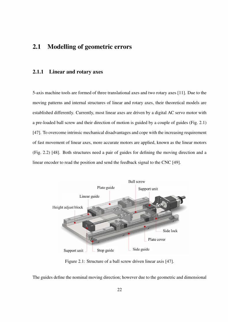
5-axis machine tools are formed of three translational axes and two rotary axes [11]. Due to the

moving patterns and internal structures of linear and rotary axes, their theoretical models are

established differently. Currently, most linear axes are driven by a digital AC servo motor with

a pre-loaded ball screw and their direction of motion is guided by a couple of guides (Fig. 2.1)

[47]. To overcome intrinsic mechanical disadvantages and cope with the increasing requirement

of fast movement of linear axes, more accurate motors are applied, known as the linear motors

(Fig. 2.2) [48]. Both structures need a pair of guides for defining the moving direction and a

linear encoder to read the position and send the feedback signal to the CNC [49].

Figure 2.1: Structure of a ball screw driven linear axis [47].

The guides define the nominal moving direction; however due to the geometric and dimensional

22

Figure 2.2: Structure of a linear motor driven linear axis [48].

imperfections in the guides and flaws in the assemblies, the poses (positions and orientations)

and motions of the linear axes are affected thus resulting in geometric errors.

Rotary axes are designed to have the rotary table or spindle rotate about designated axes, thus

having a different structure from linear axes. There are two major types of rotary axes shown

in Figs. 2.3 and 2.4, differing in their driving mechanisms. In Fig. 2.3, the driving torque is

transmitted from the hand wheel to the worm shaft, with the worm wheel connected to the

rotary table surface. In some cases, a servo motor can be applied instead of the hand wheel to

form an automatic control [50]. This structure has been used for decades due to its simplicity

and low cost. However this type of rotary axis has a number of disadvantages, some of which

include limited positioning accuracy, room needed for gears and worms, mechanical wear, etc

[51]. To resolve these problems, a better design using a torque motor has been used in 5-axis

machine tools. As depicted in Fig. 2.4, a brushless direct torque motor is applied to rotate the

table surface without the engagement of gears and worms. The use of a torque motor effectively

23

resolves the problem of backlash which appears due to gaps between worm couples when a

reverse movement (backlash) is applied [52]. The indexing position of the rotary table is read

by the rotary encoder, setting up a feedback loop in the position control. Additionally, the torque

motor provides high torque with compact shape, thus enabling its application in smaller room

compared with a worm wheel drive [53]. Despite the different internal structures, both types

have the same error components due to imperfect mechanical components and assemblies.

Figure 2.3: Structure of a worm driven rotary axis [50].

As a consequence, a broad classification has been proposed to differentiate the geometric er-

rors caused by different defects. They are the Position Dependent Geometric Errors (PDGEs)

and Position Independent Geometric Errors (PIGEs) [4, 10, 23]. Abbaszadeh-Mir et al. [54]

reported that the PDGEs, also called component errors, describe the faulty motion of moving

components. Whilst PIGEs, called location errors, appearing during assembling process, indi-

cate the position and orientation errors between the connected components.

24

Figure 2.4: Structure of a torque motor driven rotary axis [52].

2.1.2 Position Dependent Geometric Errors (PDGEs)

According to rigid body kinematics [2, 4, 17], a rigid body possesses six degrees of freedom,

determining its position and orientation in a three dimensional space [55, 56]. The six degrees

of freedom comprise three translational degrees and three rotational degrees. Correspondingly,

every degree of freedom has one component error and its value is position-dependent [22]. The

assumption of rigid body behaviour implies that the PDGE relies on the position of the moving

object with respect to a predefined reference and is a function of its nominal movement only

[22]. If the moving couple has some manufacturing defects, the accuracy of the movement is

downgraded, thus causing PDGEs. Fig. 2.5 depicts an example of a linear guideway system

whose nominal moving direction is the X-axis.

According to [10], the three principal axes that are orthogonal to each other are labelled X,

25

EXX linear positioning error along theX-axis;EYX straightness error in the Y-axis;EZX straightness error in the Z-axis;EAX angular error in the A-axis;EBX angular error in the B-axis;ECX angular error in the C-axis.

Figure 2.5: PDGEs of a linear axis (X-axis).

Y and Z, with rotary axes about each of these axes labelled A, B and C, respectively. The

six PDGE errors include two straightness error motions in the perpendicular directions to the

nominal moving direction, one positioning error motion along the moving direction and three

angular error motions about each coordinate axis. According to [10], those errors are denoted

based on the following rules.

The capital letter “E” stands for “error”, followed by a two character subscript, where the first

character is the letter representing the direction of the error and the second is the axis of motion.

PDGEs for rotary axes are defined differently due to their rotational moving patterns. For a

rotating object, it also has six degrees of freedom, thus resulting in six PDGEs—three trans-

lational PDGEs and three rotational PDGEs. For an object rotating about the C-axis, the six

PDGEs are shown in Fig. 2.6. For consistency, the PDGEs for rotary axes are named in the

same way as linear axes.

The PDGEs vary from position to position and cannot be treated as constants. Therefore re-

26

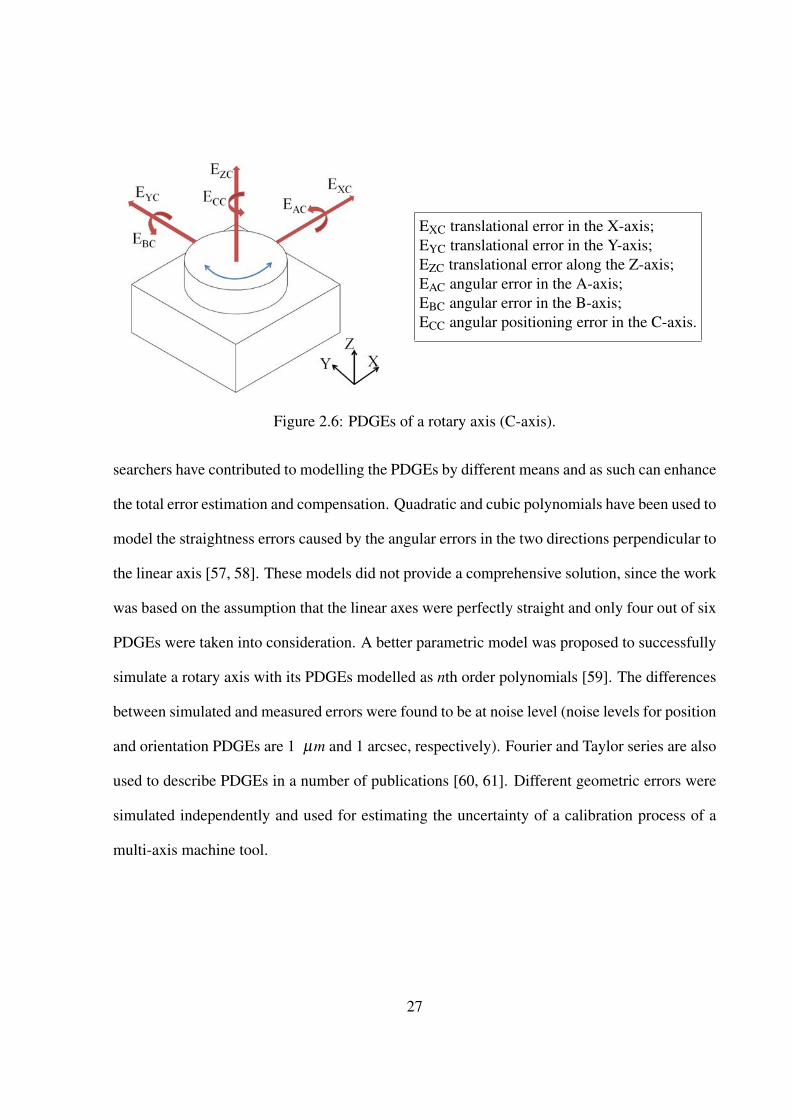
EXC translational error in the X-axis;EYC translational error in the Y-axis;EZC translational error along the Z-axis;EAC angular error in the A-axis;EBC angular error in the B-axis;ECC angular positioning error in the C-axis.

Figure 2.6: PDGEs of a rotary axis (C-axis).

searchers have contributed to modelling the PDGEs by different means and as such can enhance

the total error estimation and compensation. Quadratic and cubic polynomials have been used to

model the straightness errors caused by the angular errors in the two directions perpendicular to

the linear axis [57, 58]. These models did not provide a comprehensive solution, since the work

was based on the assumption that the linear axes were perfectly straight and only four out of six

PDGEs were taken into consideration. A better parametric model was proposed to successfully

simulate a rotary axis with its PDGEs modelled as nth order polynomials [59]. The differences

between simulated and measured errors were found to be at noise level (noise levels for position

and orientation PDGEs are 1 µm and 1 arcsec, respectively). Fourier and Taylor series are also

used to describe PDGEs in a number of publications [60, 61]. Different geometric errors were

simulated independently and used for estimating the uncertainty of a calibration process of a

multi-axis machine tool.

27

2.1.3 Position Independent Geometric Errors (PIGEs)

Position Independent Geometric Errors (PIGEs) are caused due to the imperfections of the as-

sembling process of the machine tool components [29, 54]. They can cause constant deviations

of the position and orientation of the axes. Due to the nature of the PIGEs, they are modelled

as constant values regardless of the positions where they take place. The error compositions of

linear and rotary axes are given as follows.

A prismatic joint moving along the Z-axis is illustrated to show the PIGEs of linear axes, shown

in Fig. 2.7. The reference straight line in Fig. 2.7 refers to an associated straight line fitting the

measured trajectory of points [10]. It is calculated using least squares, providing a represen-

tation of the actual condition of axes [62]. The position and orientation errors are determined

with respect to the reference straight line and the nominal coordinate frame axes.

EZ0Z linear zero position error;EA0Z error of the orientation of the Z-axisin the A-axis;EB0Z error of the orientation of the Z-axisin the B-axis.

Figure 2.7: PIGEs of a linear axis (Z-axis).

The angles between the projections of the reference straight line onto the YOZ/XOZ planes and

the Z-axis are the two orientation errors, which are also known as the squareness errors. The

third error component, “EZ0Z”, is the linear zero positioning error of the axis. In a numerical

28

controlled environment, this error can be ignored as this happens along the axis nominal moving

direction and can be compensated for by adjusting the numerical parameters [10]. Therefore in

terms of linear axes, two PIGEs are taken into consideration.

According to [10], PIGEs are labelled with the letter “E”, followed by a three-character sub-

script. The first letter in the subscript is the name of the axis referring to the direction of the

error. The second letter is a numeral “0” and the third is the moving axis.

The PIGEs of rotary axes are slightly more complicated, since not only the orientation errors,

but also the position errors need to be taken into account. Fig. 2.8 shows the error composition

for the A-axis. Each rotary axis has five PIGEs, including two position errors, two orientation

errors and one angular zero positioning error. The angular zero positioning error can be ex-

cluded from our consideration, since it can be compensated for in the encoder or the numerical

controller.

EA0A angular zero position error;EY0A position error of the A-axis in theY-axis;EZ0A position error of the A-axis in theZ-axis;EB0A orientation error of the A-axis in theB-axis;EC0A orientation error of the A-axis in theC-axis.

Figure 2.8: PIGEs of a rotary axis (A-axis).

As explained, PIGEs are treated as constants in the modelling and measuring processes. For

29

3-axis machine tools, PIGEs for each linear axes are simplified as three squareness errors be-

tween each two nominally orthogonal axes. For 5-axis machine tools, this simplification can be

achieved but is dependent upon the configuration of the machine tool [10, 29]. Therefore for

universality, the PIGEs analysed in this thesis are based on the above geometric representations

but not the simplified PIGEs for a specific machine tool configuration.

In this thesis, PIGEs and PDGEs are denoted in a simple form [4]. The simplified notations

listed in Table 2.1 have been widely used in a number of publications due to their concise

nature.

2.2 Measurement of geometric errors

As explained in Chapter 1, error identification is the initial step in the error compensation strat-

egy. After the error models are specified for all possible error sources, the next step, the error

measurement, should be carried out to determine the errors [21]. The measuring results can

provide compensation parameters for the third step: error compensation. After characterising

the errors in the given error models, error measurement strategies are developed based on the

geometric characteristics. However many errors may be superposed or overlapped in the way

that they are measured. Thus it is difficult, sometimes impossible, to decouple them in a single

measuring process. To overcome this problem, various methods using a wide variety of testing

devices are proposed to deal with different errors. These measuring methods can be generally

categorised into two approaches: direct measurements and indirect measurements [22].

30

Name of axes Errors

A-axisPDGEs

ISO EXA EYA EZA EAA EBA ECAthesis exa eya eza θxa θya θza

PIGEsISO EY0A EZ0A EB0A EC0A (EA0A)

thesis ey0a ez0a θy0a θz0a (θx0a)

B-axisPDGEs

ISO EXB EYB EZB EAB EBB ECBthesis exb eyb ezb θxb θyb θzb

PIGEsISO EX0B EZ0B EA0B EC0B (EB0B)

thesis ex0b ez0b θx0b θz0b (θy0b)

C-axisPDGEs

ISO EXC EYC EZC EAC EBC ECCthesis exc eyc ezc θxc θyc θzc

PIGEsISO EX0C EY0C EA0C EB0C (EC0C)

thesis ex0c ey0c θx0c θy0c (θz0c)

X-axisPDGEs

ISO EXX EYX EZX EAX EBX ECXthesis exx eyx ezx θxx θyx θzx

PIGEsISO EB0X EC0X (EX0X)

thesis θy0x θz0x (θx0x)

Y-axisPDGEs

ISO EXY EYY EZY EAY EBY ECYthesis exy eyy ezy θxy θyy θzy

PIGEsISO EA0Y EC0Y (EY0Y)

thesis θx0y θz0y (θy0y)

Z-axisPDGEs

ISO EXZ EYZ EZZ EAZ EBZ ECZthesis exz eyz ezz θxz θyz θzz

PIGEsISO EA0Z EB0Z (EZ0Z)

thesis θx0z θy0z (θz0z)

Table 2.1: Notations to define the geometric errors of different axes.

31

2.2.1 Direct measurements

Direct measurements refer to the measurements dealing with single errors [22]. They can be

further classified into three subcategories, shown in Fig. 2.9.

Figure 2.9: Direct measurement classification.

The material-based methods use particular precision artefacts as measuring references, for in-

stance straightedges, linear scales and step gauges [22, 63]. Dial gauges are used together with

the above measuring references to indicate the values of errors. These methods have been used

for decades and are included in national and international standards [10, 64]. However they

are still widely used because of their ease of use and simple structure. They nonetheless have

drawbacks: a major one is that the measuring accuracy relies on the accuracy of the reference

used, which is directly affected by its errors. Thus attention should be paid to the precision of

the reference when choosing the appropriate artefacts.

To overcome the above issues, laser-based measurements were developed. They use a laser

beam as the length measuring reference due to its great spatial coherence. An extensively used

32

measuring device is the laser interferometer. The measuring principle is that the wavelength

of the laser beam is employed as the length scale and transferred into the error values directly

[22]. This enables the measurement of linear positioning errors of single axes. Its application

has been expanded to enable the identification of all 21 geometric errors of 3-axis machine tools

(six PDGEs of each axis and three squareness errors between each two axes) by measuring the

positioning errors along body diagonals or other specified directions [65, 66]. With different

optics, errors including angular errors, straightness errors and squareness errors of linear axes

can be determined [10, 22, 67]. Recent innovations have enabled the positioning accuracy of

rotary axes [68, 69].

Gravity-based methods rely on the gravity field effect. The combination of a taut-wire and a

microscope are a typical example for such measuring devices [10, 22]. These types of methods

are easy to use but not suitable for horizontal planes due to the unpredictable sag of the wire

[10].

2.2.2 Indirect measurements

Indirect measuring methods work with motions involving multiple axes to analyse the machine

accuracy [22]. They can be classified into three subgroups shown in Fig. 2.10. Initially, the

indirect measurements require a specified test piece with particular geometries and shapes (e.g.

a cone frustum) mounted on the machine under test, which is then measured on a Coordinate

Measuring Machine (CMM) [70]. The result of this method is influenced by a number of

factors including the machining condition, the accuracy of the CMM being used, tool wear etc,

33

not just the geometric errors. Thus the uncertainty of the test may be greatly overestimated.

An alternative approach is to measure a machined test piece on the same machine used with

special probing systems [22]. This could partially reduce the uncertainty, but the result is still

not accurate enough due to the intrinsic errors in the machine tool.

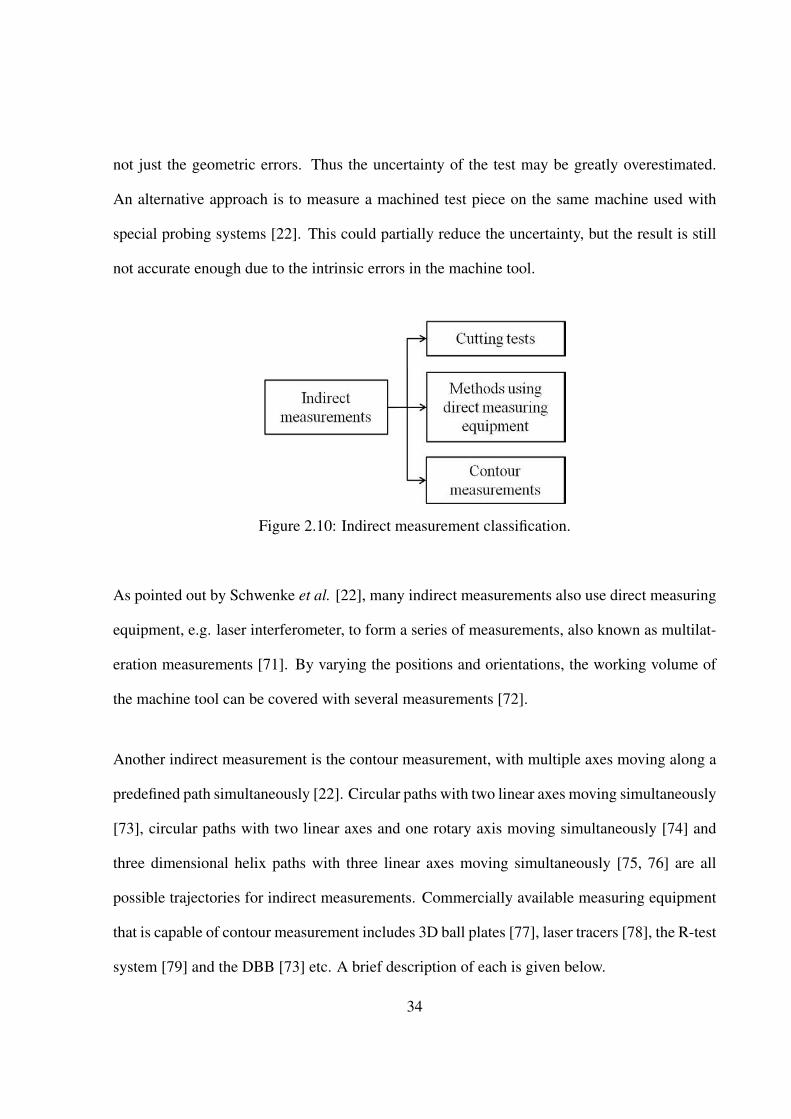
Figure 2.10: Indirect measurement classification.

As pointed out by Schwenke et al. [22], many indirect measurements also use direct measuring

equipment, e.g. laser interferometer, to form a series of measurements, also known as multilat-

eration measurements [71]. By varying the positions and orientations, the working volume of

the machine tool can be covered with several measurements [72].

Another indirect measurement is the contour measurement, with multiple axes moving along a

predefined path simultaneously [22]. Circular paths with two linear axes moving simultaneously

[73], circular paths with two linear axes and one rotary axis moving simultaneously [74] and

three dimensional helix paths with three linear axes moving simultaneously [75, 76] are all

possible trajectories for indirect measurements. Commercially available measuring equipment

that is capable of contour measurement includes 3D ball plates [77], laser tracers [78], the R-test

system [79] and the DBB [73] etc. A brief description of each is given below.

34

The 3D ball plate artefact enables the measurement of deviations in the X, Y and Z directions

at several designated points in the working volume [77]. The results can be used to derive

single geometric errors and compensate for these errors without a comprehensive machine error

model. The method is easy in theory but quite time-consuming to carry out due to the difficulties

in assuring the parallelism and straightness of the reference.

The laser tracer was developed based on displacement measuring theory to overcome the draw-

backs of the traditional laser interferometer. Rather than changing the measurement directions

every time after an error has been measured, the laser tracer is able to follow the target reflector

moving in the working volume and record the spatial displacements [78, 80]. Thus the whole

measurement can be finished with only one setup. The price for the testing equipment is rather

high (100k pounds or higher), limiting its application range.

The R-test was developed with the idea of testing rotary axes on a CMM or a 5-axis machine

tool with a setup of three linear displacement sensors and a precision ball [79]. The precision

ball is mounted in the spindle and the three non-contact displacement sensors are positioned

on the rotary table. The distance between the ball and the sensors is kept constant during the

combined movements of linear and rotary axes. Without changing the setup, the six PDGEs

of rotary axes can be diagnosed [81, 82]. Commercial software is able to compensate for the

diagnosed errors and adjust them to a desired tolerance. However, PIGEs are not covered in

the measurement. Also the method involves all five axes movements, thus relying on the high

accuracy of linear axes which requires preliminary adjustment.

Indirect measurements are established for the purpose of quick checks of machine tools, “giving

just a value for path deviation or range(s) of deviation for a tolerance check [22]”. Previous

35

researchers proposed various methods with different measuring equipment to test a number of

machine tool errors from multiple perspectives. However, these methods either require great

financial investment or need long setup time. Thus low measuring cost and high measuring

efficiency cannot be achieved. In terms of minimising the testing time and simplifying the

testing procedure, a DBB is an ideal tool for machine diagnostic testing [3, 22]. Due to its

simple structure and ease of use, the DBB is suitable for measuring the geometric accuracy of

machine tools.

2.3 DBB measurement

2.3.1 DBB system

In this thesis, a DBB system is chosen for the error measurement of the 5-axis machine tool

due to the reasons explained in Chapter 2.2. The DBB is cheap (approximately 8,000 pounds)

compared to other measuring equipment (a common laser interferometer set can cost more than

100,000 pounds). The way the DBB works is simple compared to other measuring techniques

that require hours or a day to set up and measure. Also the accuracy of the DBB can reach a

micron, which is more accurate than common CNC machine tools.

The DBB is essentially a one dimensional length measuring equipment with a precision ball

at each end, with one fixed and the other spring loaded. One typical example produced by

Renishaw plc is shown in Fig. 2.11 [73]. It includes an integrated Bluetooth wireless module

and a removable battery end cap that functions as the on-off switch. A ball bar’s nominal length

36

is 100 mm between the centres of the two balls. Extension bars of 50, 150, 300 mm in length

can be used individually or combined to provide a test radius up to 600 mm. The ball bar is

magnetised between two magnetic tool cups during testing. One tool cup is the spindle tool cup

clamped in the spindle tool holder and the other is the pivot tool cup set on the machine table.

The precision balls are connected to the tool cups by magnetic force, allowing relative rotations

only. A setup of the tool cups and the ball bar on a 3-axis machine tool is given in Fig. 2.12. The

distance between the centres of the two tool cups, namely the centres of the balls of the ball bar,

is the length captured by the ball bar. According to the ball bar specification provided by the

manufacturer [73], the resolution of the linear displacement sensor is 0.1 µm and the ball bar

accuracy is ±1.0 µm when the ambient temperature is 20◦C. Before every measurement, the

ball bar needs to be calibrated to identify its absolute length. A Zerodur R© calibrator is provided

with the ball bar tool kit for such a purpose [73].

Figure 2.11: A DBB [73].

37

Figure 2.12: A typical DBB setup [73].

2.3.2 3-axis applications

The DBB was initially designed for testing 3-axis machine tools [83]. The X-, Y- and Z-axes

are examined through three planar circular tests in the XY, YZ and ZX planes [84]. A schematic

diagram of the testing paths is given in Fig. 2.13.

In a vertical 3-axis milling machine, the DBB test includes a full circular test in the XY plane

and two partial arc tests in the YZ and XZ planes. The reason why the tests in the YZ and XZ

planes can only be conducted in partial arcs is to avoid collision of the DBB and the machine

tool. The three planar tests can be performed continuously to form a volumetric test. Up to

16 error sources including geometric and dynamic errors can be identified for three linear axes

based on the result of the volumetric test [73]. This is achieved by analysing the error plots and

comparing them with errors that have been characterised with distinctive plot shapes [85]. A

38

Figure 2.13: A schematic view of the three planar testing paths.

typical example is the effect of a squareness error between two nominally orthogonal axes. The

DBB error plot for an error-free XY planar test is a perfect circle, whilst due to the squareness

error, the shape becomes a skew ellipse (Fig. 2.14). The long axis of the oval shape aligns with

either 45◦ or 135◦ depending on the sign of the squareness error and the size of the squareness

can be determined by looking at the difference between the long axis and the nominal testing

radius.

2.3.3 5-axis applications

Recently, DBB systems have been used to evaluate the performance of 5-axis machine tools.

Geometric and dynamic errors are extensively studied with specified testing trajectories. The

research was initiated from simultaneous movements involving one rotary axis and two linear

axes, forming synchronised motions in three different directions (radial, tangential and axial)

39

Figure 2.14: DBB error plots of squareness errors. (a) squareness error= 0.01◦. (b) squarenesserror=−0.01◦.

[74]. Eight PIGEs were measured efficiently with the proposed method. With a few changes

in the testing configuration, error conditions of different types of 5-axis machine tools can be

estimated [86]. The methods have now been included in the ISO standard draft in 2012 [19].

However, since linear axes are involved in the measurements, it is difficult to separate the errors

of linear axes from the results. An idea of mimicking the cone frustum cutting test using a

DBB has been proposed to examine motion errors of rotary axes through simultaneous five axes

movements [70, 87]. Lei et al. [88] proposed a new trajectory having the A- and C-axes moving

simultaneously on a tilting rotary table type 5-axis machine tool to test the dynamic performance

of the rotary axes. Lee and Yang published a number of papers on various applications of the

DBB system. An idea of using a three dimensional hemispherical helix DBB test was proposed

to analyse the volumetric accuracy of a 3-axis machine tool [75, 76]. A four step test was

presented to evaluate the PIGEs of the A- and C-axes of a tilting rotary table type 5-axis machine

tool [5, 59, 89]. Eight PIGEs were successfully tested and with the help of a novel fixture, those

errors can be compensated for. The methods offer a possibility for machine tool measurements;

however several setups are required during testing which affects the measuring accuracy. The

40

compensation method relies on a customised fixture which cannot be achieved easily.

Most of the methods stated above require multiple setups, thus lengthening the measuring time

and inducing setup errors. The method given in this thesis is able to avoid the above drawbacks.

Also those methods are only capable of one specific type of 5-axis configuration, a generic

approach is proposed in Chapters 5 and 7 in this thesis.

2.4 Summary

In this chapter, the models and measuring methods of different types of geometric errors have

been reviewed in detail. The review started with an overview of different models of PDGEs for

both linear and rotary axes. Then corresponding models for PIGEs for linear and rotary axes

were given.

Measuring methodologies were categorised into direct and indirect measurements based on the

number of errors examined. Typical examples for both types were covered, leading to the

details of the DBB system, which is an ideal device for indirect measurement. The DBB and

its accessories were introduced to explain how it works in a 3-axis environment. The chapter

finished by briefly looking at different applications of the DBB system in 5-axis machine tools.

41

Chapter 3

Error modelling of a 5-axis machine tool

In this chapter, a machine model is established using the HTMs to evaluate the influence of

individual errors on DBB trace patterns. A number of researchers focused on the identification

of the machine tool errors with a variety of modelling techniques [17, 23, 90–94]. Most of the

work centred on the relative errors from the tool tip to the workpiece. Among them, the Homo-

geneous Transformation Matrix (HTM) method, which assumes rigid body motion, provides

a complete solution for error prediction and simulation, can therefore be used to analyse the

DBB measurement. The HTM method is helpful when evaluating the relationship between two

coordinate systems, which in this thesis are the coordinate systems affixed to the spindle and

the pivot tool cup centres. The spatial relationship is defined using the HTMs to determine the

impact of individual errors on the DBB error trace patterns. The error plots of individual errors

are generated using the given machine tool model for estimation. The machine tool model is

established with HTMs according to the test bed used in this thesis, a Hermle C600U 5-axis

42

machine tool.

3.1 HTMs of a 5-axis machine tool

With the assumption of rigid body kinematics, six degrees of freedom are assigned to each

machine tool component, including three translational degrees and three rotational degrees.

Thus, an HTM of a rigid body is given as [17, 18]:

RTC =

R3×3 T3×1

0 0 0 S

=

rix riy riz tx

r jx r jy r jz ty

rkx rky rkz tz

0 0 0 1

where the superscript R represents the reference coordinate frame that the result is expressed

with respect to and the subscript C is the coordinate frame that the results are transferred from.

R3×3 represents the orientation matrix of the rigid body coordinate frame C with respect to the

reference coordinate frame R. T3×1 represents the translation from the coordinate frame C to

the reference coordinate frame R. The bottom row represents the scale factor. When dealing

with rigid bodies, S = 1 and it is given as [0 0 0 1] .

With the given HTM expression, the ideal kinematic movements of the linear axes (X, Y and Z)

with respect to the reference coordinate frame R can be expressed as:

43

RTX,ideal =

1 0 0 Xm +XX

0 1 0 XY

0 0 1 XZ

0 0 0 1

; RTY,ideal =

1 0 0 YX

0 1 0 Ym +YY

0 0 1 YZ

0 0 0 1

;

RTZ,ideal =

1 0 0 ZX

0 1 0 ZY

0 0 1 Zm +ZZ

0 0 0 1

where Xm, Ym and Zm denote the kinematic linear position of the X-, Y- and Z-axes respectively

with respect to the reference coordinate system R. XX , XY and XZ are the constant offsets in the

X, Y and Z directions of the origin of the X-axis coordinate systems relative to the reference

coordinate system R, respectively. Similar notation is used for YX , YY and YZ in RTY,ideal, and

ZX , ZY and ZZ in RTZ,ideal.

Similarly, the HTMs of the rotary axes (A, B and C) are:

RTA,ideal =

1 0 0 AX

0 cosθa −sinθa AY

0 sinθa cosθa AZ

0 0 0 1

; RTB,ideal =

cosθb 0 sinθb BX

0 1 0 BY

−sinθb 0 cosθb BZ

0 0 0 1

;

44

RTC,ideal =

cosθc −sinθc 0 CX

sinθc cosθc 0 CY

0 0 1 CZ

0 0 0 1

where θa, θb and θc are the kinematic angular positions of the A-, B- and C-axes respectively

with respect to the reference coordinate system R. AX , AY and AZ are the constant offsets in the

X, Y and Z directions of the origin of the A-axis coordinate systems relative to the reference

coordinate system R, respectively. Similar notation is used for BX , BY and BZ in RTB,ideal, and

CX , CY and CZ in RTC,ideal.

The actual position and orientation of the axes are affected due to the PIGEs. To clearly identify

all error sources, the HTM of each link element or servo driven axis is represented as a product

of basic HTMs, including the HTMs of the kinematic parameters and the PIGEs. For exam-

ple, the C-axis rotary table rotates nominally about the C-axis centre line and its position and

orientation are affected by two position PIGEs ex0c and ey0c, and two orientation PIGEs θx0c

and θy0c. The PIGEs of the C-axis can be seen from Fig. 3.1, which depicts the perfect C-axis

table coordinate frame OC and the actual C-axis table coordinate frame OCE. So the actual

position and orientation of the C-axis rotary table can be expressed with respect to the reference

coordinate frame R as:

RTC,actual = Eex0c ·Eey0c ·Eθx0c ·Eθy0c ·RTC,ideal

45

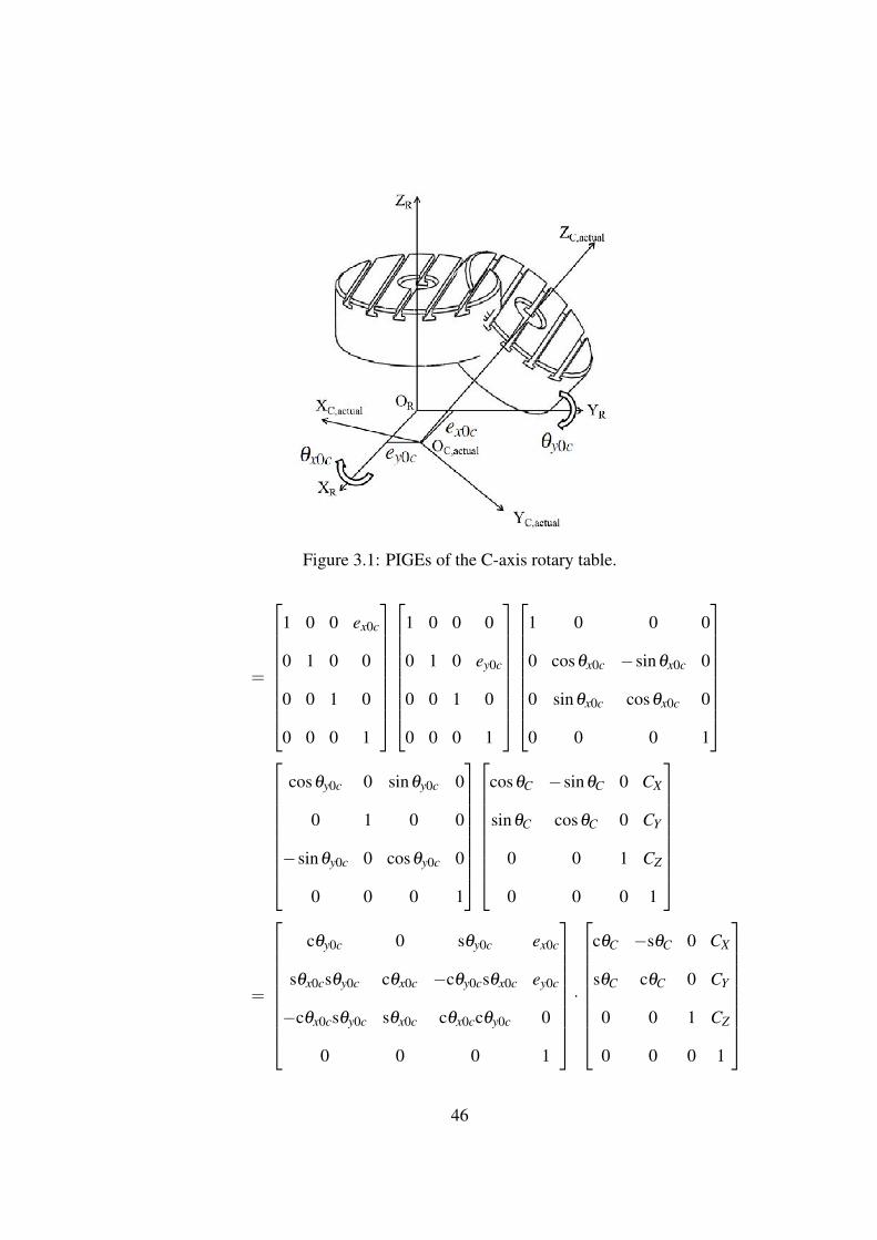
Figure 3.1: PIGEs of the C-axis rotary table.

=

1 0 0 ex0c

0 1 0 0

0 0 1 0

0 0 0 1

1 0 0 0

0 1 0 ey0c

0 0 1 0

0 0 0 1

1 0 0 0

0 cosθx0c −sinθx0c 0

0 sinθx0c cosθx0c 0

0 0 0 1

cosθy0c 0 sinθy0c 0

0 1 0 0

−sinθy0c 0 cosθy0c 0

0 0 0 1

cosθC −sinθC 0 CX

sinθC cosθC 0 CY

0 0 1 CZ

0 0 0 1

=

cθy0c 0 sθy0c ex0c

sθx0csθy0c cθx0c −cθy0csθx0c ey0c

−cθx0csθy0c sθx0c cθx0ccθy0c 0

0 0 0 1

·

cθC −sθC 0 CX

sθC cθC 0 CY

0 0 1 CZ

0 0 0 1

46

where s and c are abbreviations for sin and cos respectively.

Since the orientation PIGEs are all less than 1◦ [95, 96], the small angle approximation assump-

tion (sin(θ) ≈ θ , cos(θ) ≈ 1, when the angle θ < 1◦) is applied and second order errors are

neglected. Thus the error matrix for the C-axis rotary table can be simplified as follow

RTC,actual =

1 0 θy0c ex0c

0 1 −θx0c ey0c

−θy0c θx0c 1 0

0 0 0 1

·

cθC −sθC 0 CX

sθC cθC 0 CY

0 0 1 CZ

0 0 0 1

=

cθc −sθc θy0c CX +θy0cCZ + ex0c

θx0cθy0ccθc + sθc −θx0cθy0csθc + cθc −θx0c θx0cθy0cCX +CY −θx0cCZ + ey0c

−θy0ccθc +θx0csθc θy0csθc +θx0ccθc 1 −θy0cCX +θx0cCY +CZ

0 0 0 1

The HTM provides a possibility to combine the inaccuracies of a moving axis with its nominal

kinematic motion. The machine tool structure is thus able to be decomposed into a series of

HTMs, describing the actual relative position and orientation of each moving axis [21]. Ac-

cording to [17, 18, 21], if n rigid bodies are connected in series and the relative HTMs between

each two consecutive axes are known, the pose of the tool tip (the nth coordinate frame) with

respect to the zero coordinate frame 0 can be deduced by sequential multiplication of all HTMs:

0Tn =n

∏i=1

(i−1Ti

)= 0T1

1T22T3 · · ·n−1Tn (3.1)

where pTq (p,q = 0,1,2 · · ·n) is the HTM representing the transformation from coordinate

47

frame q to p.

3.2 Error evaluation of DBB tests

After identifying the HTMs for each individual axes, the next step is to build up the machine tool

model with them. Fig. 3.2 illustrates the test bed used in this study, a Hermle 5-axis machine

tool.

Figure 3.2: A schematic view of the Hermle C600U 5-axis machine tool structure.

A Hermle C600U tilting rotary table 5-axis machine tool consists of three linear axes X, Y and

Z, and two rotary axes A and C, which are the rotations about the X- and Z-axes respectively

[97]. This type of 5-axis machine tool can be seen as a combination of a 3-axis machine tool

48

configured in a standard Cartesian coordinate system and a tilting rotary table at the lower part

of the machine body.

Fig. 3.3 shows the machine tool kinematic structure with affixed coordinate frames on different

machine tool components. Fig. 3.4 indicates the relative position between each two adjacent

coordinate frames. The kinematic chain consists of prismatic and rotary joints in a serial se-

quence. One end of the kinematic chain is the tool tip on the spindle side (spindle tool cup

centre). The spindle tool cup is attached to the spindle, mounted on the Z-axis slide. The Z-axis

slide translates vertically relative to the X-axis slide, which moves vertically with respect to

the Y-axis slide. The Y-axis slide is a moving gantry across the machine bed, supported by the

frame with a pair of parallel guides. The other end of the kinematic chain starts from the pivot

tool cup attached to the C-axis rotary table. The pivot rotates with the rotary table about the

C-axis centre line. The C-axis rotary table is designed on top of the A-axis tilting table, which

is installed in the machine frame with a pair of pneumatic cylinders.

The modelling starts from defining the reference coordinate frame R. The point where the A-

and C-axes nominally intersect is chosen as the origin of the reference coordinate frame OR.

The X-, Y- and Z-axes of the reference coordinate frame are chosen to be parallel to the X-, Y-

and Z-slide moving directions. When the A-axis tilting table is set to be flat (the servo controlled

angular position θa = 0◦), the A-axis coordinate frame overlaps with the reference coordinate

frame R. The C-axis rotary table coordinate frame is attached to the C-axis table surface, with

its origin OC having the same X and Y coordinates as OR in the reference coordinate frame R.

The distance between OC and OR along the Z-axis direction of the reference coordinate frame

R is ZCA. The spindle tool cup centre is selected as the origin of the spindle coordinate frame S.

49

Figure 3.3: Coordinate frames assignment for the components in the kinematic chain.

The coordinate frame has offsets of X1, Y1 and Z1 in the X-, Y- and Z-directions of the reference

coordinate frame R respectively.

The DBB pivot (OPOW in Figs. 3.3 and 3.4) is attached to the C-axis rotary table surface and

its coordinate frame is determined to have the same Z height as OC with respect to the reference

coordinate frame R. However the X and Y positions are dependent upon the test setups since

the pivot is located differently when testing different axes. As an example, the distance between

OP and OC is R in the Y-direction in Figs. 3.3 and 3.4. The workpiece coordinate frame W is

assigned to the centre of the pivot tool cup. The distance from the centre of the pivot tool cup

to the bottom of the pivot along the axis of the pivot, namely OW OP in Figs. 3.3 and 3.4, is

denoted as H.

50

Figure 3.4: Relationships between different coordinate frames.

In this case, the linear axes X, Y and Z are considered free of errors, since linear axes are easy to

measure with current methods and compensate for with current CNC controllers [10, 36, 37, 40].

Therefore only the position of the spindle tool cup with respect to the reference coordinate frame

R is taken into account in this machine tool model.

Errors in the two tool cups are not taken into consideration in the modelling stage since they

can be eliminated or compensated for in the error calculation process [95]. Thus the errors in

the pivot tool cup position are not considered in the modelling stages.

51

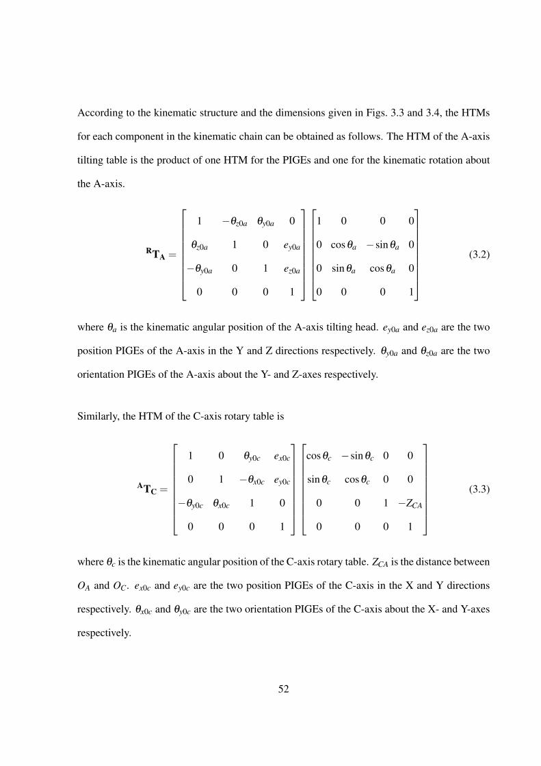
According to the kinematic structure and the dimensions given in Figs. 3.3 and 3.4, the HTMs

for each component in the kinematic chain can be obtained as follows. The HTM of the A-axis

tilting table is the product of one HTM for the PIGEs and one for the kinematic rotation about

the A-axis.

RTA =

1 −θz0a θy0a 0

θz0a 1 0 ey0a

−θy0a 0 1 ez0a

0 0 0 1

1 0 0 0

0 cosθa −sinθa 0

0 sinθa cosθa 0

0 0 0 1

(3.2)

where θa is the kinematic angular position of the A-axis tilting head. ey0a and ez0a are the two

position PIGEs of the A-axis in the Y and Z directions respectively. θy0a and θz0a are the two

orientation PIGEs of the A-axis about the Y- and Z-axes respectively.

Similarly, the HTM of the C-axis rotary table is

ATC =

1 0 θy0c ex0c

0 1 −θx0c ey0c

−θy0c θx0c 1 0

0 0 0 1

cosθc −sinθc 0 0

sinθc cosθc 0 0

0 0 1 −ZCA

0 0 0 1

(3.3)

where θc is the kinematic angular position of the C-axis rotary table. ZCA is the distance between

OA and OC. ex0c and ey0c are the two position PIGEs of the C-axis in the X and Y directions

respectively. θx0c and θy0c are the two orientation PIGEs of the C-axis about the X- and Y-axes

respectively.

52

The transformation from the pivot coordinate frame P to the C-axis rotary table coordinate

frame C is given as:

CTP =

1 0 0 0

0 1 0 −R

0 0 1 0

0 0 0 1

(3.4)

where R is the distance between OP and OC in the Y direction of the C-axis coordinate system.

The position of OW in the pivot coordinate frame P is

PVOW = [0 0 H 1]T (3.5)

and the position of OS in the reference coordinate frame R is

RVOS = [−X1 −Y1 Z1 1]T . (3.6)

According to [17], a close kinematic chain can be illustrated as a “transform graph” (Fig. 3.5).

Each short vertical line represents a coordinate frame affixed on selected machine components

in the kinematic chain. The arrow pointing from one vertical line to another stands for a trans-

formation from one coordinate to the next. Thus the position of the tool tip with respect to the

reference coordinate system R can be obtained based on the given HTMs and the transform

graph.

For instance, the position of the pivot tool cup on the C-axis rotary table with respect to the

reference coordinate system R can be obtained by starting at the base of the RVOW and listing

53

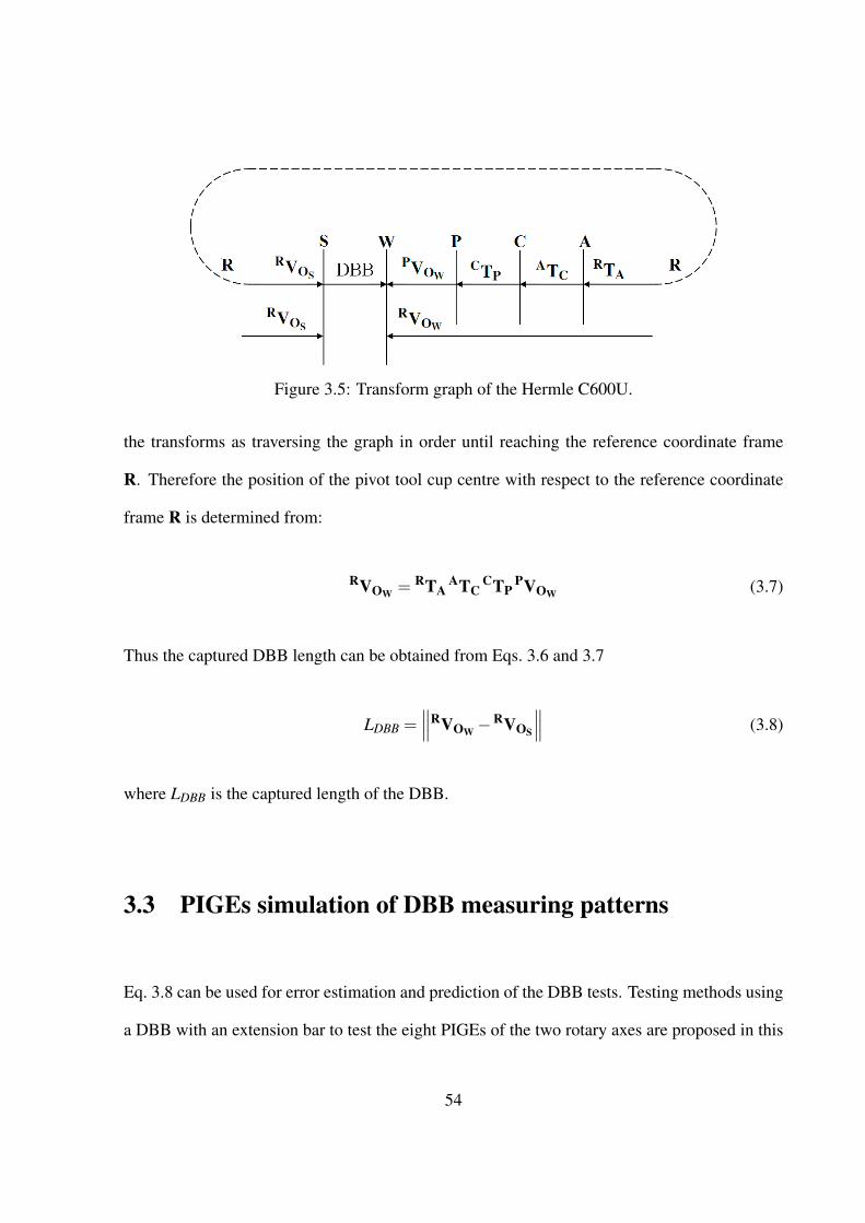
Figure 3.5: Transform graph of the Hermle C600U.

the transforms as traversing the graph in order until reaching the reference coordinate frame

R. Therefore the position of the pivot tool cup centre with respect to the reference coordinate

frame R is determined from:

RVOW = RTAATC

CTPPVOW (3.7)

Thus the captured DBB length can be obtained from Eqs. 3.6 and 3.7

LDBB =∥∥∥RVOW−

RVOS

∥∥∥ (3.8)

where LDBB is the captured length of the DBB.

3.3 PIGEs simulation of DBB measuring patterns

Eq. 3.8 can be used for error estimation and prediction of the DBB tests. Testing methods using

a DBB with an extension bar to test the eight PIGEs of the two rotary axes are proposed in this

54

thesis. The simulated error plots were generated with Eq. 3.8 to observe individual error impacts

on DBB measurements. There are three different testing methods proposed in Chapters 4 to 6

respectively. The method presented in Chapter 5 is used for simulation. The simulation process

can be used for testing methods presented in Chapters 4 and 6. When applying the model to

methods in Chapters 4 and 6, the spindle tool cup position and the pivot position, namely RVOS

and CTP, need to be adapted to the corresponding test setups. RVOS and CTP can be obtained

from Fig. 4.3 and Table 4.1 for the method given in Chapter 4, and Fig. 6.1 and Table 6.2 for

the method given in Chapter 6.

Based on the four steps of the test proposed in Chapter 5, some key specifications of the machine

tool and the DBB as well as simulation conditions are given in Table 3.1. The position PIGEs

are set as 10 µm and the orientation PIGEs as 0.01◦ for the simulation. The four steps of the

proposed method are shown in Fig. 3.6.

Table 3.1: Simulation condition.

Parameters ValuesNominal DBB length (mm) 100Nominal extended DBB length (mm) 150ex0c ey0c ey0a ez0a ( µm) 10θx0c θy0c θy0a θz0a (degree) 0.01Test radius R (mm) 100Distance between OC and OR ZCA (mm) 75Pivot tool cup centre height from the pivot bottom H (mm) 75

When testing the A-axis, the A-axis tilting table is only able to rotate from −20◦ to 70◦, there-

fore −20◦ ≤ θa ≤ 70◦ in Eq. 3.2. When testing the A-axis without an extension bar (Fig. 3.6),

55

Figure 3.6: The testing method in Chapter 5. (a) the A-axis test without an extension bar. (b)the A-axis test with an extension bar. (c) the C-axis test without an extension bar. (d) the C-axistest with an extension bar.

Eqs. 3.4 and 3.6 are given as

CTP =

1 0 0 0

0 1 0 R

0 0 1 0

0 0 0 1

(3.9)

RVOS = [0 0 0 1]T . (3.10)

56

When testing the A-axis with an extended DBB, Eqs. 3.4 and 3.6 are given as

CTP =

1 0 0 0

0 1 0 R

0 0 1 0

0 0 0 1

(3.11)

RVOS = [−D 0 0 1]T . (3.12)

where −D is the distance between OS and OR in the X direction in order to fit the length of

the extended DBB. When using a 150 mm DBB, OSOR can be deduced using the Pythagrorean

theorem

D =√

1502−1002 = 50√

2. (3.13)

Thus

RVOS =[−50√

2 0 0 1]T

. (3.14)

Similar to the A-axis tests, the C-axis is also tested in two steps, without and with an extension

bar. For the C-axis test without the extension bar, Eqs. 3.4 and 3.6 are given as

CTP =

1 0 0 R

0 1 0 0

0 0 1 0

0 0 0 1

(3.15)

RVOS = [0 0 0 1]T . (3.16)

57

When testing the C-axis with an extended DBB, Eqs. 3.4 and 3.6 are given as

CTP =

1 0 0 R

0 1 0 0

0 0 1 0

0 0 0 1

(3.17)

RVOS = [0 0 D 1]T . (3.18)

where D is the distance between OS and OR in the Z direction in order to fit the length of the

extended DBB. When using a 150 mm DBB, OSOR can be deduced from Eq. 3.13. Thus

RVOS =[0 0 50

√2 1

]T. (3.19)

With the modified CTP and RVOS given above, the length of DBB can be evaluated with Eq. 3.8.

For instance when testing the A-axis without an extended DBB, LDBB can be obtained with

Eqs. 3.2, 3.3, 3.5, 3.9, 3.10 as follow. Using MATLAB, symbolic matrix multiplication is

achieved without any rounding errors in the calculations.

LDBB =∥∥∥RVOW−

RVOS

∥∥∥

58

= ((ey0a + cθa(ey0c +ZCAθx0c)+ZCAsθa +θz0a(ex0c−ZCAθy0c)−H(sθa

−θy0cθz0a +θx0ccθa)−R(sθa(θx0ccθc +θy0csθc)− cθacθc +θz0asθc))2

+((θz0acθa−θy0asθa)(ey0c +ZCAθx0c)− ex0c +ZCAθy0c−H(θy0c

+θx0c(θz0acθa−θy0asθa)+θy0acθa +θz0asθa)+ZCA(θy0acθa +θz0asθa)

+R(sθc− (θy0acθa +θz0asθa)(θx0ccθc +θy0csθc)+ cθc(θz0acθa

−θy0asθa)))2 +(ez0a + sθa(ey0c +ZCAθx0c)−H(θy0aθy0c− cθa +θx0csθa)

−ZCAcθa−θy0a(ex0c−ZCAθy0c)+R(cθcsθa +θy0asθc + cθa(θx0ccθc

+θy0csθc)))2)(

12 )

(3.20)

When testing the A-axis with an extended DBB, LDBB can be obtained with Eqs. 3.2, 3.3, 3.5,

3.11, 3.14:

LDBB =∥∥∥RVOW−

RVOS

∥∥∥= (((θz0acθa−θy0asθa)(ey0c +ZCAθx0c)− ex0c +ZCAθy0c−50

√2−H(θy0c

+θx0c(θz0acθa−θy0asθa)+θy0acθa +θz0asθa)+ZCA(θy0acθa

+θz0asθa)+R(sθc− (θy0acθa +θz0asθa)(θx0ccθc +θy0csθc)

+ cθc(θz0acθa−θy0asθa)))2 +(ey0a + cθa(ey0c +ZCAθx0c)+ZCAsθa

+θz0a(ex0c−ZCAθy0c)−H(sθa−θz0aθy0c +θx0ccθa)−R(sθa(θx0ccθc

+θy0csθc)− cθacθc +θz0asθc))2 +(ez0a + sθa(ey0c +ZCAθx0c)

−H(θy0aθy0c− cθa +θx0csθa)−ZCAcθa−θy0a(ex0c−ZCAθy0c)

+R(cθcsθa +θy0asθc + cθa(θx0ccθc +θy0csθc)))2)(

12 )

(3.21)

59

Eqs. 3.20 and 3.21 enable the generation of error plots due to individual PIGEs: only the PIGE

under evaluation is set to a predefined value given in Table 3.1, all the other PIGEs are set to

zeros. Figs. 3.7 and 3.8 illustrate the DBB trace patterns affected by different PIGEs of the two

steps of the A-axis test.

From the figures it can be observed that, compared with the standard circles (black circles in

each subfigures), all simulated patterns are eccentric circles apart from Figs. 3.7 (c) and (d).

This is due to the fact that when testing the rotary axes without the extension bar, the spindle

ball of the DBB is placed at the origin of the reference coordinate frame R, thus orientation

PIGEs do not influence the patterns. The generated DBB trace patterns can be used as a fast

indication of PIGEs, which is useful when evaluating machine tool conditions. Also, with the

given machine tool model, estimation of individual error impact on the machine tool volumetric

accuracy becomes possible. This approach can be adapted to other testing schemes in this thesis

and other types of 5-axis machine tools by changing the parameters in the HTMs of the machine

tool components.

3.4 Summary

In this chapter, HTMs for individual machine tool components with the PIGEs specified in

Chapter 2 were developed. Then a machine tool model based on the test bed used in this thesis

was established with the given HTMs. The machine tool model was used for generating DBB

error plots, which were presented based on the A-axis test of the method proposed. From the

error plots, it can be concluded that the HTM model of the machine is correct. Individual error

60

Figure 3.7: DBB error trace patterns of the A-axis test without the extension caused by (a) ey0a,(b) ez0a, (c) θy0a and (d) θz0a (1div.= 5 µm).

plots indicated the impact of each PIGE on the DBB trace patterns, which could be used for

machine tool condition evaluation and error prediction.

61

Figure 3.8: DBB error trace patterns of the A-axis test with the extension caused by (a) ey0a, (b)ez0a, (c) θy0a and (d) θz0a (1div.= 5 µm).

62

Chapter 4

DBB tests

To identify and characterise PIGEs of rotary axes of a 5-axis machine tool, a measuring ap-

proach using a DBB is presented in this chapter. The proposed measuring method consists

of four tests for two rotary axes: the A-axis tests with and without an extension bar and the

C-axis tests with and without an extension bar. For tests without the extension bar, position

errors embedded in the A- and C-axes are measured first. Then these position errors can be

used with the results of tests with the extension bar, to obtain the orientation errors in the A-

and C-axes based on the given geometric model. All tests are performed with only one axis

moving, thus simplifying the error analysis. The idea of testing the rotary axes is to isolate the

position and orientation errors and measure them separately. Errors existing in the equipment

setup process are measured and calibrated with conventional DBB tests. The proposed method

is implemented on a 5-axis machine tool to validate the approach.

The testing procedure is carried out with the assumption that the X-, Y- and Z-axes are within

63

tolerance and hence will not introduce any significant errors. This is because current controllers

are proficient at compensating for the geometric errors of linear axes but not capable of dealing

with errors in rotary axes [36, 37, 40].

As discussed in Chapter 1, 5-axis machine tools have many possible configurations. In this the-

sis, a tilting rotary type 5-axis machine tool, which is extensively used in industry is employed

as the test bed. The majority of this type of machine tools are configured with an indexing

rotary table above a tilting table [11].

4.1 Four steps of tests

4.1.1 Testing equipment

As explained in Section 3.2, the 5-axis machine tool consists of three linear axes at the upper part

and two rotary axes at the lower part of the machine tool. A sectional view of the mechanisms

is given in Fig. 4.1.

The three linear axes are driven by ball screws and guided by linear guides. An image of the

linear axes driving structure is given in Fig. 2.1. In order to hold the heavy moving slide and

the spindle, the Y-axis slide is designed to be supported by three linear guides to ensure its

precision.

The worm design of the A-axis is shown in Fig. 4.2. The rotational driving force is transmitted

64

Figure 4.1: Hermle C600U 5-axis machine tool [97].

from a servo motor to the worm shaft then to the worm wheel connected with the A-axis table.

The A-axis tilting table is supported by a pair of pneumatic cylinders on each side, whilst the

C-axis rotary table is directly driven by a torque motor (Fig. 2.4).

The DBB and its accessories used in this study have been introduced in Chapter 2.

65

Figure 4.2: The A-axis driving structure.

4.1.2 DBB setups

Before discussing the setup of the DBB system, the reference coordinate system needs to be

defined. The origin of the reference coordinate system is defined as the intersection of the ideal

A- and C-axes when they are at their zero positions. The three axes of the reference coordinate

system are parallel to the three linear axes X, Y and Z of the machine tool coordinate system.

The setup process starts with attaching the pivot to the A-axis tilting table away from the origin

of the reference coordinate system. The centre of the spindle tool cup is then aligned with the

A-axis. The two balls of the DBB, namely the spindle ball and the table ball, are attached

to the spindle and pivot tool cups respectively. This configuration ensures any error captured

is caused by the misalignment between the reference straight line of the A-axis and its ideal

66

position. Also, since the centre of the spindle tool cup lies on the ideal A-axis in the plane

where the trajectory lies, orientation errors do not have any significant impact on the result,

which means the analysed errors are purely the position errors of the A-axis. In order to avoid

any collision of the DBB and the machine tool, the A-axis tilting movement is restricted to

−20◦ to +70◦.

Figure 4.3: 4 stage rotary axes test set-up on a 5-axis machine tool. (a) A-axis test without anextension bar. (b) A-axis test with an extension bar. (c) C-axis test without an extension bar. (d)C-axis test with an extension bar.

To fit the 150 mm DBB with an extension bar, a displacement of the spindle tool cup in the

negative X-axis direction is applied (Fig. 4.3(b)). The DBB in this step moves with its axis

67

tilted with respect to the YZ plane of the reference coordinate system. The same tilting angle of

the A-axis from −20◦ to +70◦ is applied and the trajectory of the DBB is a quarter of a conic

surface.

Since the DBB length has been changed, a recalibration process of the extended length is needed

prior to installing the DBB. A calibrator made of Zerodur R© with zero thermal expansion co-

efficient is used for the recalibration [73]. The absolute length of the extended DBB can be

obtained.

The third step is carried out for the purpose of testing the C-axis position errors. Unlike the

A-axis tests, the C-axis rotary table is able to be driven through 360◦ with the DBB. The centre

of the spindle tool cup is set to be at the origin of the reference coordinate system. The pivot

is placed away from the C-axis by a DBB nominal length in the X direction of the reference

coordinate system. This ensures only the position errors will be reflected in the result, without

any influence from the orientation errors of the C-axis. However, as the C-axis rotary table

is on top of the A-axis table, position errors in the Y-axis direction of A-axis will affect the

accuracy of the C-axis. So the effect of the A-axis errors should be taken into consideration

when calculating the C-axis PIGEs.

In the final step, the orientation errors in the C-axis are tested with the same extended DBB.

Similar to the idea of testing the A-axis orientation errors, the DBB rotates in a full circle with

its axis tilted with respect to the XY plane of the reference system.

68

4.1.3 Error elimination before start

The raw data, which is the length changes of the DBB, needs to be converted into coordinate

values in the corresponding local coordinate frames for later use. However two error sources

appear which affect the accuracy of the test. One is the set-up precision of the spindle tool cup

and the other is the position of the pivot tool cup. To ensure the spindle tool cup centre line

aligns with the main spindle axis, a dial gauge with a magnetic base mounted on the machine

table is used to keep the runout in the horizontal plane within the machine tolerance, which is

1 µm. The spindle tool cup is clamped in the spindle tool holder after the horizontal accuracy

is adjusted to the machine tolerance. The centre of the spindle tool cup is then measured in the

Z direction with respect to the Z-axis zero point with a tool setting probe attached on the table.

The test datum is set using the measured spindle tool cup position.

The positional accuracy of the centre pivot is obtained by using a planar circular DBB test

around the pivot tool cup centre. The C-axis set-up procedures are taken as an example to show

the process of eliminating the starting position errors. Errors in the placement of the pivot in

the Y or X direction will influence the precision since the deviations are in the error sensitive

directions [74].

Let P0 = (X0,Y0,Z0) be the ideal start position and P′0 the actual start position. An error of the

rotational angle δe will occur (Fig. 4.4), and is given by:

δe = tan−1(

P0P′0jP0P′0i+100

)(4.1)

where P0P′0 is the vector form P0 to P′0, i and j are the unit vectors of the X- and Y-axes respec-

69

Figure 4.4: Influence of inaccurate start position.

tively, and 100 is the nominal radius of the DBB table ball trajectory.

The vector P0P′0 is determined by performing a conventional XY planar circular test around the

starting position. The centre offsets in the X and Y directions are then used to correct the actual

starting position P′0. A similar strategy can be applied to the A-axis for the elimination of the

start position error. For the A-axis start error correction, a partial arc test in the YZ plane is

performed after set-up to derive centre offsets in the Y- and Z-axes directions.

4.2 Error analysis

For tests with and without an extension bar, the processes of modelling and analysing the errors

are different. However, the analysis for the same type of test (with or without the extension bar)

70

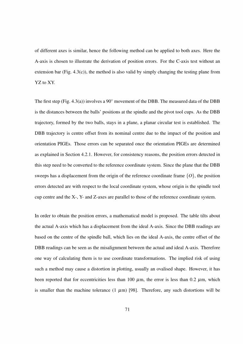
of different axes is similar, hence the following method can be applied to both axes. Here the

A-axis is chosen to illustrate the derivation of position errors. For the C-axis test without an

extension bar (Fig. 4.3(c)), the method is also valid by simply changing the testing plane from

YZ to XY.

The first step (Fig. 4.3(a)) involves a 90◦ movement of the DBB. The measured data of the DBB

is the distances between the balls’ positions at the spindle and the pivot tool cups. As the DBB

trajectory, formed by the two balls, stays in a plane, a planar circular test is established. The

DBB trajectory is centre offset from its nominal centre due to the impact of the position and

orientation PIGEs. Those errors can be separated once the orientation PIGEs are determined

as explained in Section 4.2.1. However, for consistency reasons, the position errors detected in

this step need to be converted to the reference coordinate system. Since the plane that the DBB

sweeps has a displacement from the origin of the reference coordinate frame {O}, the position

errors detected are with respect to the local coordinate system, whose origin is the spindle tool

cup centre and the X-, Y- and Z-axes are parallel to those of the reference coordinate system.

In order to obtain the position errors, a mathematical model is proposed. The table tilts about

the actual A-axis which has a displacement from the ideal A-axis. Since the DBB readings are

based on the centre of the spindle ball, which lies on the ideal A-axis, the centre offset of the

DBB readings can be seen as the misalignment between the actual and ideal A-axis. Therefore

one way of calculating them is to use coordinate transformations. The implied risk of using

such a method may cause a distortion in plotting, usually an ovalised shape. However, it has

been reported that for eccentricities less than 100 µm, the error is less than 0.2 µm, which

is smaller than the machine tolerance (1 µm) [98]. Therefore, any such distortions will be

71

insignificant. Before carrying out the experiment, a measurement using a dial indicator assures

the misalignment is less than 100 µm. Therefore, in this thesis the coordinate transformation

method is employed for calculating the misalignment.

The Y and Z coordinates of the ith point lying on the DBB table ball trajectory, Pi = (Xi,Yi,Zi),

are used to calculate the position errors using Least Squares [98]. Furthermore, for a constant

feed rate, the points are considered uniformly distributed, and we may set

θi =iN·Θ

Yi = (Rn +δi) · cos(θi +δe)

Zi = (Rn +δi) · sin(θi +δe)

where δi and θi are the captured DBB length variations and the rotational angle of the ith point

respectively. N is the total number of captured points. Θ is the total angle of rotation. The

nominal length of the DBB is represented by Rn; Yi and Zi are the coordinates of the table ball

centre respectively. θe is the error in the initial start position and is obtained with Eq. 4.1.

The position errors are then determined from:

(y− ey0a)2 +(z− ez0a)

2 = R2

where ey0a and ez0a are the position errors in Y- and Z-axes directions respectively. R is the

radius of the least squares fitted circle. Further, the distance between the point Pi and the rotation

72

centre di can be calculated from:

(Yi− ey0a)2 +(Zi− ez0a)

2 = d2i .

Least Squares Fitting minimises the sum of the squared differences between the distance di and

the fitting radius R. Therefore let

f (a,b,c) =N

∑i=0

(d2i −R2)2 =

N

∑i=0

(Y 2i +Z2

i +aYi +bZi + c)2

where

a =−2 · ey0a

b =−2 · ez0a

c = e2y0a + e2

z0a−R2.

To obtain the minimum value of the above equation, total derivatives of f (a,b,c) with respect

to a, b and c are given, which can be written in matrix form

N∑

i=0Y 2

i

N∑

i=0YiZi

N∑

i=0Yi

N∑

i=0YiZi

N∑

i=0Z2

i

N∑

i=0Zi

N∑

i=0Yi

N∑

i=0Zi N

·

a

b

c

=

N∑

i=0(Y 3

i +YiZ2i )

N∑

i=0(Y 2

i Zi +Z3i )

N∑

i=0(Y 2

i +Z2i )

and

73

ey0a

ez0a

R

=

−1

2a

−12b

12

√a2 +b2−4c

4.2.1 Tests with an extension bar

For the purpose of making the orientation errors evident, a different configuration is applied.

As shown in Fig. 4.3(b), an extension bar (50 mm) is added to the DBB in order to amplify the

effect of the orientation errors. The X-axis is driven in the negative direction to fit the longer

length without moving the table pivot. An exaggerated diagram to illustrate the error is given in

Fig. 4.5.

Figure 4.5: An exaggerated schematic view highlighting the PIGEs of the A-axis.

74

The position errors calculated in the first step can be denoted as the length O′P in Fig. 4.5, where

the point O′ is the ideal rotation centre whilst the point P is the offset centre due to the position

errors. In the second step with the extension bar, the spindle tool cup centre is shifted to S′.

This is achieved by driving the X-axis to the designated position. The spindle tool cup is kept

in the spindle, thus its centre position relative to the spindle centre line and the zero position of

the Z-axis does not change. With the assumption that all linear axes are within tolerances, the

accuracy of the spindle tool cup position can be guaranteed.

In order to transfer the captured lengths of the DBB to the bottom plane of the cone, a normal

line passing through S′ is made, having an intersection point E with the bottom surface formed

by EPi. In the triangle4S′PiE,

S′P2i = S′E2 +EP2

i .

Expressing Li (captured DBB lengths) in terms of the radius of the bottom circle of the cone

EPi, fitted using least squares, the distance EP can be obtained from Eqs. 4.2 to 4.4.

(y−YEP)2 +(z−ZEP)

2 = R2f (4.2)

where YEP and ZEP are the Y and Z components of EP respectively. R f is the radius of the least

squares fitted circle.

(Yi−YEP)2 +(Zi−ZEP)

2 = EP2i (4.3)

g(m,n, p) =N

∑i=0

(EP2i −R2)2 =

N

∑i=0

(Y 2i +Z2

i +mYi +nZi + p)2 (4.4)

where

m =−2 ·YEP

75

n =−2 ·ZEP

p = Y 2EP +Z2

EP−R2f .

Finally equate the total derivatives of g(m,n, p) with respect to m, n and p to 0. Thus YEP, ZEP

and R f are given as

YEP =−m2

ZEP =−n2

R f =12

√m2 +n2−4p.

Since SP and S′E are normal to the bottom plane, the orientation errors of S′E are the same as

those errors of SP. Therefore the orientation errors θy0a and θz0a can be calculated as:

θy0a = tan−1 ZO′E

‖S′O′‖;

θz0a = tan−1 YO′E

‖S′O′‖.

where YO′E and ZO′E are the Y and Z components of O′E respectively. Here the length EP+

PO′ is used instead of O′E, since O′E cannot be determined without knowing θy0a and θz0a.

Although EP and PO′ are not in the same plane, The resulting difference of the substitution ∆

can be determined from:

∆ = (EP+PO′)−O′E = PO′(1

cosθy0a cosθz0a−1). (4.5)

Tests without the extension bar showed that θy0a and θz0a are smaller than 1◦ (Assuming the

centre offsets captured in steps 1 and 3 are all due to orientation PIGEs, and the results of the

76

orientation PIGEs are smaller than 1◦). This suggests that ∆ is less than 10−8 mm which is

small enough to neglect.

4.3 Experimental validation

The proposed method is tested on a Hermle C600U 5-axis machine tool, whose structure is

shown in Fig. 4.1. An overshoot angle before and after the data capture arc is given in all tests

[73]. The purpose of the angular overshoot is to allow the machine to accelerate to the required

feed rate before the DBB passes through the data capture arc, and to decelerate before the feed

out movement is performed. For the C-axis tests, a recommended 45◦ was thus applied. For

the A-axis tests, however, since the DBB only travels in a 90◦ arc, big overshoot angles are no

longer feasible. According to [73], it is recommended that some angular overshoot is included,

even if the shooting angle is as small as a few degrees. Hence a 2◦ overshoot angle was chosen

in order to get as many data points as possible. The specification of the test is given in Table 4.1.

Before every test the machine tool is warmed up for 20 minutes according to the standard

warming-up procedure recommended in [10]. The four steps of the tests take approximately

30 min including the set-up process.

Figures before and after compensation of the A- and C-axes are given in Figs. 4.6 and 4.7 to

show the effectiveness of the proposed method. After the diagnosed PIGEs are compensated

to the target axes, residual errors still exist in the A- and C-axes. However the value of the

remaining errors are within tolerance (< 1 µm), shown in Fig. 4.8 for both axes. Tests with

77

Table 4.1: Specification of DBB tests.

Parameters ValueNominal length Rn (mm) 100.0000Calibrated length Rc (no extension bar) (mm) 99.9881Calibrated length Re (with extension bar) (mm) 149.9946Overshoot angle (degree) (C-axis) 45◦

Overshoot angle (degree) (A-axis) 2◦

Testing feed rate F(mm/min) 500

different feed rates were carried out to identify the remaining error sources. It has been observed

that with an increasing feed rate, the residual errors increase. Since the geometric errors are not

effected by the feed rate, the residual errors are likely to be caused by dynamic errors, which

are feed rate influenced [88].

The test was repeated 10 times until the repeatability was within the tolerances (1 µm for po-

sition PIGEs and 1′′ for orientation PIGEs). The repeatability tests were carried out consecu-

tively without changing the testing setups or conditions. Since every step can be conducted very

quickly (< 1min), the thermal condition of the machine itself and its environment only change

slightly, this will not induce significant thermal variations.

Averages and standard deviations of all testing results are calculated based on the repeatability

tests, given in Tables 4.2 and 4.3. Among those PIGEs, ey0c and θx0c are fairly large compared

to the other errors. Nonetheless they can also be compensated with the tested values and the

compensated results (Fig. 4.8) are within tolerances. Therefore the reason of ey0c and θx0c being

relatively large might be due to the worn condition of the bearing in the C-axis. The results need

to be compared with those inspected with other methods to determine their correctness. An

established method can be considered as an alternative to test the PIGEs of rotary axes, which

will be given in Chapter 6.

78

Figure 4.6: A-axis test result with (blue) and without compensation (red) (mm).

Figure 4.7: C-axis test result with (blue) and without compensation (red) (mm).

79

Figure 4.8: Residual error of the A- (blue) and C-axis (red) test with compensation (mm).

Table 4.2: Test results for position PIGEs.

Parameters Average (mm) Standard deviation (mm)ey0a 0.0342 0.00008ez0a -0.0353 0.00037ex0c 0.0013 0.00015ey0c -0.0525 0.00060

Table 4.3: Test results for orientation PIGEs.

Parameters Average (′′) Standard deviation (′′)θy0a 6.62 0.557θz0a 1.89 0.388θx0c -22.32 0.489θy0c -3.75 0.527

80

4.4 Summary

This chapter presents a new procedure using a DBB to identify the PIGEs of a 5-axis machine

tool using new testing paths for the A- and C-axes. The four steps of the procedure consist

of tests with and without the use of an extension bar for both the A- and C-axes. Since the

C-axis rotary table is designed on top of the A-axis tilting table, the tests start from the A-axis

measurement for the simplicity in error separation. The first testing step, without an extension

bar, is to determine the position errors. Then, using a 50 mm extension bar, the orientation

errors can be obtained. Similar steps are used for the C-axis tests after compensating for the

A-axis errors. The procedure is then validated using a 5-axis machine tool.

By controlling the rotary axes individually, the analysis of PIGEs is simplified since the result

only reflects the error condition of the axis under test. Other advantages of the proposed method

are that it requires no additional fixturing, and is applicable to other types of 5-axis machine

tools. The testing setup for the C-axis presented in this chapter can be used on the rotary axis

table in the RTTTR type 5-axis machine tools as demonstrated in Chapter 1.

81

Chapter 5

A method of testing the accuracy of a

5-axis machine

In Chapter 4, the two rotary axes were tested with the DBB pivot located at different positions

on the tilting rotary table. Such a method requires several setups of the pivot which induce

complexities. For example, each reposition of the pivot requires a process of exchanging another

tool holder from the tool magazine, clamping the pivot tool cup into the tool holder and attaching

it to the desired location. The setup process takes a few minutes thus increasing the measuring

time. In addition, every time the position of the pivot is reset, the pivot tool cup needs to

be recalibrated with the conventional DBB tests as explained in Section 4.1.3. The method

proposed in Chapter 4 required two planar circular tests to obtain the deviations in the pivot

tool cup for error calculation. To reduce the number of conventional DBB tests and enhance the

testing efficiency, a method involving just one pivot setup will be presented in this chapter. This

82

method can be used in those configurations where the two rotary axes are integrated together, i.e.

both rotary axes on the spindle side or on the table side. In terms of the calculation process of

the PIGEs, there exists another complexity in the previous method: the errors of the A-axis were

given with respect to the local coordinate system thus requiring a conversion to express them

with respect to the reference coordinate system. To avoid excessive calculation, the method in

this chapter measures all PIGEs in the reference coordinate system, thus no conversion of the

coordinates is required.

5.1 Experimental design

In this test, the two rotary axes (the A- and C-axes) were examined in four steps, shown in

Fig. 5.1. The DBB was placed with one ball in the spindle tool cup at the origin of the reference

coordinate system (RCS) and the other ball in the pivot tool cup away from the nominal C-axis

by a distance of Rnom. The A-axis was first driven in a 90◦ arc, from −20◦ to +70◦ to avoid

any collision of the DBB and the machine tool. Such configuration ensures any error captured

is caused by the misalignment between the reference straight line of the A-axis and its ideal

position. Also, since the centre of the spindle tool cup lies on the ideal A-axis in the trajectory

plane, orientation errors do not have any significant impact on the results, which means the

analysed centre offsets of the trajectory are purely position errors of the A-axis.

In the second step, the DBB length was extended by 50 mm using an extension bar. To fit the

150 mm DBB, a displacement of the spindle tool cup in the negative X direction was applied

(Fig. 5.1(b)). The same tilting angle of the A-axis from −20◦ to +70◦ was applied and the

83

Figure 5.1: 4 steps of Test 1. (a) the A-axis test without an extension bar. (b) the A-axis testwith an extension bar. (c) the C-axis test without an extension bar. (d) the C-axis test with anextension bar.

trajectory of the DBB formed a quarter of a conic surface.

The third step is to test the C-axis without the extension bar (Fig. 5.1(c)): the C-axis rotary table

was rotated through a 360◦ circle with the DBB. The spindle ball was kept stationary with its

centre aligning with the nominal C-axis. The trajectory of the DBB was in the XY plane of the

RCS, which ensures only the position PIGEs will be reflected in the results. However, as the

C-axis rotary table is on top of the A-axis table, position errors in the Y-axis direction of the

A-axis will affect the accuracy of the C-axis tests. Hence the testing results of the A-axis should

be removed from the errors of the C-axis.

84

In the final step, the C-axis table was rotated in the same 360◦ planar trajectory (Fig. 5.1(d)).

With the 50 mm extension bar on the DBB, the orientation PIGEs were obtained.

5.2 Error analysis

The first and third steps use the same idea as in Chapter 4 to measure the centre offsets of the

trajectory from its nominal centre as the position PIGEs. Least squares fitting is applied to

minimise the sum of the differences between the fitting radius and the distances between the

rotation centre and each measured point. By this means, the position PIGEs (ey0a and ez0a of

the A-axis and ex0c and ey0c of the C-axis) can be determined.

For the second and fourth steps, the extension bar is applied to make the orientation PIGEs

evident. A diagram to illustrate the exaggerated errors is given in Fig. 5.2. The second step

which is the A-axis test with the extension bar is explained herein, the same model can be

adopted in the fourth step.

The centre offsets calculated in the first step is denoted as OP, where the point O is the ideal

centre of rotation and the point P is the offset centre due to the position PIGEs. With the

extension bar, the spindle ball is moved to point S. In order to transfer the captured lengths Li

between the spindle tool cup centre S and the ith point Pi = (Xi,Yi,Zi) lying on the trajectory

(red circle), a normal line passing through S is drawn, having an intersection point E with the

85

Figure 5.2: A geometric model for the orientation errors in the A-axis test with the extensionbar.

bottom surface formed by EPi. In the triangle4SEPi

SP2i = SE2 +EP2

i .

Expressing Li in terms of the radius of the bottom circle of the cone EPi, fitted using least

squares, the distance EP can be obtained from Eqs. 5.1 to 5.3 [95].

(y−YEP)2 +(z−ZEP)

2 = R2f (5.1)

86

where YEP and ZEP are the Y and Z components of EP respectively. R f is the radius of the least

squares fitted circle.

(Yi−YEP)2 +(Zi−ZEP)

2 = EPi2 (5.2)

g(m,n, p) =N

∑i=0

(EPi2−R2

f )2 =

N

∑i=0

(Y 2i +Z2

i +mYi +nZi + p)2 (5.3)

where

m =−2 ·YEP

n =−2 ·ZEP

p = Y 2EP +Z2

EP−R2f .

Finally equate the total derivatives of g(m,n, p) with respect to m, n and p to 0. Thus YEP and

ZEP are given as

YEP =−m2

ZEP =−n2

Therefore from Eq. 5.1 we have:

R f =12

√m2 +n2−4p.

Since SE is normal to the bottom plane and hence parallel to the A-axis reference straight line,

the orientation errors of SE are the same as those errors of the A-axis reference straight line.

87

Therefore the orientation errors θya and θza can be calculated as:

θy0a = tan−1(

YOE

‖SO‖

)

θz0a = tan−1(

ZOE

‖SO‖

)where YOE and ZOE are the Y and Z components of OE respectively. SO is the distance between

the spindle ball and the origin of the RCS. Here the length OE is approximated as EP+PO. The

approximation results in negligible errors which have been addressed in Chapter 4. The above

method can help to identify the position and orientation PIGEs of the A- and C-axes. Table 5.1

lists the errors identified in each step, where ey0a,bot , ez0a,bot , ex0c,bot and ey0c,bot are the respec-

tive distances between the centres of the bottom circles and the origins of the corresponding

local coordinate systems.

Table 5.1: Errors included in each step of the test.

Steps Test description Position PIGEs Orientation PIGEsstep 1 the A-axis test without the ex-

tension barey0a ez0a

θy0a θz0a

step 2 the A-axis with the extensionbar

ey0a,bot ez0a,bot

step 3 the C-axis without the extensionbar

ex0c ey0c ey0aθx0c θy0c

step 4 the C-axis with the extensionbar

ex0c,bot ey0c,bot ey0a,bot

88

5.3 Experimental validation

The proposed method was implemented on the same Hermle C600U 5-axis machine tool as in

Chapter 4. Test specifications have been given in Table 4.1. The difference between the two

methods in Chapters 4 and 5 is the location of the pivot and the number of setups. In Chapter 4,

the pivot was first mounted on the A-axis tilting table surface then moved to the C-axis rotary

table surface. Whilst in this chapter the pivot was installed on the C-axis rotary table surface

without further changes in its position.

A 20 min warm up of the machine tool was carried out before each test according to [10]. Like

the method in Chapter 4, the test was repeated until the repeatability was within the tolerance

(1 µm for position PIGEs and 1′′ for orientation PIGEs). Averages and standard deviations of

all results given in Tables 5.2 and 5.3 were calculated based on the repeatability tests.

Table 5.2: Testing results for position PIGEs.

Parameters Average (mm) Standard deviation (mm)ey0a 0.0353 0.00034ez0a −0.0334 0.00029ex0c 0.0013 0.00015ey0c −0.0529 0.00049

Table 5.3: Testing results for orientation PIGEs.

Parameters Average (′′) Standard deviation (′′)θy0a −1.29 0.427θz0a 1.20 0.9072θx0c −22.28 0.409θy0c 4.48 0.579

To show the effectiveness of the proposed method, the estimated PIGEs were compensated for

the raw data. Figures before and after compensation of the test results are given in Figs. 5.3 and

89

Figure 5.3: A-axis test result with (blue) and without compensation (red) (mm).

Figure 5.4: C-axis test result with (blue) and without compensation (red) (mm).

90

5.4.

The position PIGEs obtained with the method given in Chapter 4 are close to the ones given

in this chapter (< 1µm for both axes), whilst the orientation PIGEs vary, especially θy0a and

θy0c. In the next chapter, a published method will be presented to verify both methods given in

Chapters 4 and 5 [5]. In order to verify the results obtained in Chapters 4 and 5, they will be

compared to the results obtained using the method given in [5].

5.4 Summary

A method with only one setup of the pivot on the tilting rotary table to test the two rotary axes

A and C is proposed in this chapter. The method evolves from the one presented in Chapter

4. The testing idea is similar but the number of setups has been reduced: the rotary axes were

first tested without the extension bar to determine the position PIGEs, then with the extension

for the orientation PIGEs without moving the pivot. With the minimal number of setups, the

conversion of the PIGEs with respect to the RCS is avoided and the measuring efficiency is

enhanced.

Compared with the method given in Chapter 4, the results of this method showed agreement

in position PIGEs but discrepancies in the orientation PIGEs θy0a and θy0c. To get a better

understanding of the disagreement, an established method will be presented in the next chapter

for comparison and verification purposes.

91

Chapter 6

Verification of the proposed method

The idea of using a DBB with and without an extension bar to determine the PIGEs of a single

rotary axis in two steps has been given in Chapters 4 and 5. For verification purposes, a pub-

lished testing model [5] is given to test the same PIGEs with a DBB, then compared with the

results with those obtained in the previous chapters. The effectiveness of the published method

can be seen from the difference between the DBB error plots with and without the compensation

of the identified PIGEs. In this chapter, the two rotary axes A and C were tested separately, and

the position and orientation PIGEs were measured at different testing positions. Experimental

details and results are given.

92

6.1 Four steps of tests

6.1.1 Experiment setups

The test was carried out in four steps, two for each axis, as depicted in Fig. 6.1. When testing

the A-axis, two pivot positions 1 and 2 (Fig. 6.1(a) and (b)) which are symmetric with respect

to the YZ plane of the RCS were chosen for the first and second steps respectively. The pivot

was attached to the A-axis tilting table away from the origin of the RCS. The centre of the

spindle tool cup was aligned with the A-axis, having the same X coordinate as the pivot tool

cup centre. During both measurements, the spindle ball was kept stationary and aligning with

the nominal A-axis, whilst the table ball tilted with the A-axis table about the A-axis. Only the

A-axis rotated during testing, providing a precise evaluation of position PIGEs of the A-axis.

Positions 3 and 4 (Fig. 6.1(c) and (d)) were chosen for the third and fourth steps of the C-axis

tests with different Z heights. When testing position 3, the pivot was directly attached to the

C-axis table surface whilst for position 4, a step block and gauge blocks were needed to lift up

the pivot, as shown in Fig. 6.2. It can be seen in both steps that the spindle ball and the table

ball were positioned with the same height above the C-axis table. The table ball rotated with

the C-axis table and the centre of the spindle ball was kept stationary, aligning with the C-axis.

As the accuracy of both tool cups are error prone, calibration of the tool cups were conducted

after setting the pivot positions. Since the tool cup fixed in the spindle tool holder remained un-

changed, the distance from the tool cup centre to the Z-axis zero position was ensured accurate,

as explained in Section 4.1.3. Also the axis of the tool cup centre line and the rotational axis

93

Figure 6.1: 4 steps of the DBB tests. (a) position 1 of the A-axis test. (b) position 2 of theA-axis test. (c) position 3 of the C-axis test. (d) position 4 of the C-axis test.

of the spindle was measured and adjusted to be within tolerance. In terms of the centre pivot

position, conventional DBB measurements were carried out to determine the deviations in the

Y and Z directions of the A-axis tests and deviations in the X and Y directions of the C-axis

tests, respectively.

94

Figure 6.2: the C-axis test on a higher level.

6.1.2 Error analysis

The planar circular tests were conducted to measure the centre offsets of the four circular tra-

jectories at the four positions given in Fig. 6.1. The centre offsets, namely the local position

PIGEs, are not completely identical to the ones measured with respect to the RCS due to the

influences of the orientation PIGEs. Since the rotary axes reference straight lines do not rely

on the coordinate system chosen, the orientation PIGEs are the same regardless of testing po-

sitions. The relationships between the local position PIGEs and the ones measured in the RCS

can be expressed as

ey0a,lcs = ey0a,rcs +DA tanθz0a

ez0a,lcs = ez0a,rcs +DA tanθy0a

ex0c,lcs = ex0c,rcs +DC tanθy0c +DC tanθy0a

ey0c,lcs = ey0c,rcs +DC tanθx0c

95

where the subscripts “lcs” and “rcs” indicate the position PIGEs are expressed with respect to

the LCS and RCS respectively.

Schematic views of the results from the A- and C-axes tests are given in Figs. 6.3 and 6.4. DA

is the distance from position 1 to the origin of the RCS along the X direction of the RCS, thus

OO1 = OO2 = DA

O1O2 represents the nominal A-axis, intersecting the YZ planes of the LCS at points O1 and

O2. In Fig. 6.3, O′1 and O′2 are the intersections of the actual A-axis and the YZ planes of the

LCS respectively. D1 and D2 are the vectors from O1 to O′1 and O2 to O′2 respectively.

Figure 6.3: The two trajectories of the A-axis tests at Positions 1 and 2.

Thus the orientation PIGEs of the A-axis are given as

θy0a = tan−1(

e′′z0a− e′z0a

2DA

)

θz0a = tan−1(e′′y0a− e′y0a

2DA

)96

Figure 6.4: The two trajectories of the C-axis tests at Positions 3 and 4.

where e′y0a and e′z0a are the Y and Z components of D1 respectively and e′′y0a and e′′z0a are the Y

and Z components of D2 respectively.

In Fig. 6.4, the ideal C-axis passes through the origin of the RCS O (O3) and intersects the XY

plane of the LCS at O4. Correspondingly, the actual C-axis intersects the XY planes of the RCS

and LCS at O′3 and O′4 respectively. DC is the distance from position 3 to position 4 along the Z

direction of the RCS, thus

OO4 = DC.

The vectors from O3 to O′3 and from O4 to O′4, i.e. D3 and D4, are not only influenced by the

C-axis PIGEs but also the PIGEs of the A-axis. Therefore

θx0c = tan−1(e′y0c− ey0c

DC

)

θy0c = tan−1(

e′x0c− tanθy0a ·DC− ex0c

DC

)

97

where ex0c and ey0c are the X and Y components of D3 respectively and e′x0c and e′y0c are the X

and Y components of D4 respectively.

The above analysis indicates the errors obtained in each step of the test, which are listed in

Table 6.1. The orientation PIGEs of each rotary axis can be deduced from the position PIGEs.

Table 6.1: Errors included in each step of the test.

Steps Test description Position PIGEs Orientation PIGEsstep 1 position 1 of the A-axis test e′y0a e′z0a θy0a θz0astep 2 position 2 of the A-axis test e′′y0a e′′z0astep 3 position 3 of the C-axis test ex0c ey0c ey0a

θx0c θy0cstep 4 position 4 of the C-axis test e′x0c e′y0c ey0a

6.1.3 Experimental validation

The proposed method was implemented on the same Hermle C600U 5-axis machine tool with

the same testing conditions as the methods of Chapters 4 and 5. The testing specifications are

given in Table 6.2. The four step tests were conducted following the 20 min warm up session.

The results were recorded after the test repeatability was within tolerance (1 µm for position

PIGEs and 1′′ for orientation PIGEs). The results are given in Tables 6.3 and 6.4. Figs. 6.5 and

6.6 illustrate the DBB trace patterns before and after compensation.

98

Table 6.2: Specification of DBB tests.

Parameters ValueA-axis rotation range −20◦ to +70◦

C-axis rotation range 450◦

Nominal length Rn (mm) 100.0000Calibrated length Rc (no extension bar) (mm) 99.9881Overshoot angle (degree) (C-axis) 45◦

Overshoot angle (degree) (A-axis) 2◦

Testing feed rate F(mm/min) 500Offset DA (mm) 550Offset DC (mm) 78

Table 6.3: Testing results for position PIGEs.

Parameters Average Standard deviationey0a 0.0335 mm 0.00008 mmez0a −0.0356 mm 0.0002 mmex0c 0.0014 mm 0.00012 mmey0c −0.0513 mm 0.0006 mm

Table 6.4: Testing results for orientation PIGEs.

Parameters Average Standard deviationθy0a 7.23′′ 0.130′′

θz0a 2.94′′ 0.063′′

θx0c -26.03′′ 0.785′′

θy0c -14.38′′ 0.665′′

99

Figure 6.5: A-axis test result with (blue) and without compensation (red) (mm).

Figure 6.6: C-axis test result with (blue) and without compensation (red) (mm).

100

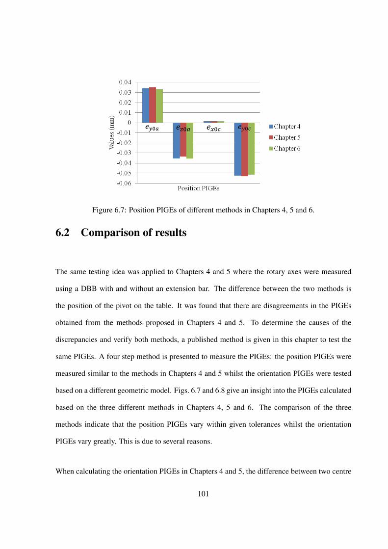
Figure 6.7: Position PIGEs of different methods in Chapters 4, 5 and 6.

6.2 Comparison of results

The same testing idea was applied to Chapters 4 and 5 where the rotary axes were measured

using a DBB with and without an extension bar. The difference between the two methods is

the position of the pivot on the table. It was found that there are disagreements in the PIGEs

obtained from the methods proposed in Chapters 4 and 5. To determine the causes of the

discrepancies and verify both methods, a published method is given in this chapter to test the

same PIGEs. A four step method is presented to measure the PIGEs: the position PIGEs were

measured similar to the methods in Chapters 4 and 5 whilst the orientation PIGEs were tested

based on a different geometric model. Figs. 6.7 and 6.8 give an insight into the PIGEs calculated

based on the three different methods in Chapters 4, 5 and 6. The comparison of the three

methods indicate that the position PIGEs vary within given tolerances whilst the orientation

PIGEs vary greatly. This is due to several reasons.

When calculating the orientation PIGEs in Chapters 4 and 5, the difference between two centre

101

Figure 6.8: Orientation PIGEs of different methods in Chapters 4, 5 and 6.

offset circles was used to obtain the deviations caused by the PIGEs [99]. The difference be-

tween the local centre offsets of the same axis in different steps is only a few microns. These

local centre offsets are affected by the DBB measuring uncertainty (1µm), thus the difference

of those offsets may fluctuate. This results in the disagreement of the orientation errors obtained

in the four steps using the methods given in Chapters 4 and 5.

For instance, in Chapter 4 when testing the A-axis, the first step without the extension bar gives

the position PIGEs, which is denoted as O′P in Fig. 4.5. In the second step the extended DBB

lengths were converted to the bottom of the cone, and the centre offsets of the cone bottom

circle are denoted as EP. In Eq. 4.5, O′E was approximated as O′P+PE

O′E = O′P+PE = O′P−EP.

which is the difference between the two centre offsets.

Constrained by the measuring uncertainty of the DBB, the value of O′E is affected, thus causing

102

the fluctuations in the orientation PIGEs. In order to improve the measuring accuracy as much

as possible, longer extension bars are recommended to magnify the effect of the orientation

PIGEs [5], however additional calibrators are required for calibrating the DBB length.

Also straightness errors and the positioning variability of linear axes may affect the accuracy

of the results. Relevant research indicated that the above causes can result in loss of accuracy

of the tests [5, 89]. This can be explained from the perspective of the linear guideways. For

most 5-axis machine tools, the sizes of the components being machined determine the amount

of wear on different positions of the guideway [100]. The majority of the components being

machined are small to medium sized with respect to the machine tool working volume. The

result is that the central part of the guideways are used the most [100]. Therefore, taking the

Hermle C600U as an example, the central parts of the X and Y guideways which are close to

the origin of the RCS, have the highest probability to be used and worn. Using the central parts

of the X- and Y-axes to place and measure the pivot may result in additional errors. Whilst for

the method proposed in this chapter, the central parts of the linear axes are avoided to perform

the measurements of the A-axis. Therefore the PIGEs of the A-axis in this chapter agree with

the ones in Chapter 4.

However, it can be seen that variations of the values of θx0c and θy0c exist between Chapters 4,

5 and 6. One reason, as explained previously, is due to the small difference between the centre

offsets of the two circles obtained with and without the extension bar. Another reason is that the

height difference between the third and fourth steps of the method in this chapter is not large

enough to differentiate between the two local position PIGEs when testing the C-axis. Thus

the orientation PIGEs in this chapter are easily affected by the uncertainty of the measurement.

103

According to [5], larger distances between the two positions is recommended to improve the

uncertainty of the measured orientation PIGEs. However, since the test bed employed in this

thesis is a small-sized machine tool, the height used in the fourth step is close to the Z-axis

upper limit, a larger distance between the two positions is not possible.

The focus of this thesis is on characterising the PIGEs of rotary axes. Since the characteristics

of the observed PIGEs in the methods of Chapters 4 and 5 are similar to those of Chapter 6 (cf.

Figs. 4.6 and 4.7 in Chapter 4, Figs. 5.3 and 5.4 in Chapter 5, and Figs. 6.5 and 6.6 in Chapter

6), the methods are in agreement.

6.3 Summary

In order to justify the results given in Chapters 4 and 5, a verified method testing the eight PIGEs

of the two rotary axes A and C using a different geometric model was presented in this chapter.

For each axis, two different positions along the rotational axis were selected as the testing

locations. Local position PIGEs were measured with respect to the LCS and orientation PIGEs

were obtained using these position PIGEs. Comparisons of the results of the three methods in

Chapters 4, 5 and 6 are given. The results showed a good agreement in position PIGEs for all

three methods, but discrepancies in orientation PIGEs, especially for θy0a and θy0c. The reasons

are due to worn conditions of linear axes and limited testing ranges.

104

Chapter 7

Conclusions and future work

The thesis has been concerned with the identification and characterisation of position indepen-

dent geometric errors (PIGEs) of rotary axes of 5-axis machine tools using a double ball bar

(DBB).

In 5-axis machine tools, two rotational degrees of freedom allow the cutter to orient with respect

to the workpiece. Additional flexibility induced by the rotary axes enables machining complex

shapes with fewer setups of the workpiece. However, the rotational degrees may cause addi-

tional errors to the machine tools, thus calibration of the rotary axes are needed to improve the

accuracy of 5-axis machine tools. To this end, the background knowledge in 5-axis machine

tools and their error sources were introduced, and some key processes to reduce the errors, in-

cluding error elimination and error compensation were discussed. Motivated by the prospect

of improving the accuracy of 5-axis machine tools, the procedures of the error compensation

scheme was studied extensively. Being one of the major error sources in a 5-axis machine tool,

105

geometric errors were considered in this thesis. More specifically, PIGEs which are due to im-

perfections during the assembly process of the machine tool were studied in detail. Research

objectives were then given to highlight the main goals of the thesis, including identifying and

characterising the PIGEs of rotary axes of 5-axis machine tools using a DBB, and simulating

the identified errors for prediction and verification purposes.

Some key issues in modelling the geometric errors of linear and rotary axes were addressed

in Chapter 2. Both PDGEs and PIGEs were examined; structural diagrams were given for

demonstration. Measurement of different geometric errors based on their characteristics were

discussed in Section 2.2. To gain a systematic understanding of those errors, a broad classifica-

tion was given to categorise the measurements into direct and indirect measurements according

to the number of errors being tested. A number of commonly used direct/indirect measuring

approaches were introduced briefly. Among them, a simple and efficient way to characterise

the linear axes using a DBB was presented. The conventional DBB tests were demonstrated

as well as their limitations. To fully exploit a DBB’s potential, an idea of applying a DBB to

characterising errors in 5-axis machine tools was developed and previous published methods

for both 3- and 5-axis machine tools were revisited.

Preparatory to the development of the new methods, the error modelling of a 5-axis machine

tool with the HTMs was presented in Chapter 3 to estimate individual error impacts on the DBB

trace patterns. First some basics in the HTMs were introduced for prismatic and rotational

joints. Then a theoretical machine model was established by affixing coordinate frames to

selected machine tool components (Figs. 3.3 and 3.4). Sequential multiplication of the HTMs

representing the kinematic motion and the PIGEs matrices defines the machine tool volumetric

106

position from the tool tip to the workpiece side. The simulated DBB error trace patterns based

on the measuring method given in Chapter 6 due to individual PIGEs were generated with

Eq. 3.8.

A novel DBB measuring method was proposed in Chapter 4 to characterise four PIGEs of each

rotary axis of a 5-axis machine tool including two position PIGEs and two orientation PIGEs

as discussed in Section 2.1.3. A strength of the methods is only the rotary axis under test was

moving during testing, thus greatly simplifying the error separation. The idea was to test the

position PIGEs of each rotary axis separately, having the DBB motion trajectory perpendicular

to the rotary axis straight line. Such testing setup ensured that only the local position PIGEs

were involved in the deviation of the motion trajectory. Orientation PIGEs were measured

based on a given geometric model (Fig. 4.5), where the orientation PIGEs could be obtained

by having an extended DBB rotating in the same pattern as the position PIGEs. This is based

on the fact that the values of position PIGEs rely on the testing location whilst the orientation

PIGEs remain unchanged regardless of testing location.

Before performing the measurements, setup errors in the spindle and pivot tool cups were con-

sidered. The alignment of the centre line of the spindle tool cup with the main spindle axis

was ensured by using a dial gauge to measure its runout in the horizontal plane. Whilst the

vertical position was ensured accurate since the spindle tool cup was clamped in the tool holder

before setting the datum. Imprecision in the pivot tool cup centre was measured with the con-

ventional DBB planar tests, detected errors were then considered in the calculation process for

compensation.

Since the method in Chapter 4 required two setups of the pivot which reduced the measuring

107

efficiency, a method with only one pivot setup was proposed in Chapter 5 for error character-

isation. The difference between the two methods is the pivot location: in Chapter 4, the pivot

was first located on the A-axis tilting table then moved to the C-axis rotary table surface; whilst

in Chapter 5, the pivot was mounted on the C-axis table surface for all testing steps. The test-

ing procedures for both methods were similar: the position PIGEs were tested using a 100 mm

DBB for each rotary axes then the orientation PIGEs were examined with an extended DBB

(150 mm). Measuring efficiency was enhanced in practice, verification of the above methods is

nonetheless required to show their effectiveness. Therefore an established method using a DBB

to characterise the same PIGEs was given in Chapter 6 [5]. Due to its validity, it serves as a

verification of the other two methods.

Each rotary axis was diagnosed in Chapter 6 with the DBB placed at different positions along

the axis reference straight line. Thus four setups of the pivot were required to estimate the eight

PIGEs of the two rotary axes A and C. Results of the three different methods were presented for

comparison. The position PIGEs vary within tolerance among the three methods, whilst value

fluctuation can be observed in the orientation PIGEs. This is mainly due to several reasons

including:

• the small difference between the centre offsets of circles obtained with and without the

extension bars on the DBB;

• the straightness errors and the positioning variability of linear axes;

• the distance between different steps in the method of Chapter 6.

The proposed methods in this thesis are not used for precision calibration of 5-axis machine

108

tools; their value lies in the fast characterisation of the PIGEs: if the results of the test show the

accuracy of the machine tool is within its tolerance, no further checking is needed; otherwise

detailed examination using more precise equipment should be carried out to determine where

the flaw exists in the machine. The method can be applied to other types of 5-axis machine tools,

like the one shown in Fig. 1.1(a). When testing the C-axis (Fig. 7.1), a flat fixture attached to the

spindle head is used to fix the spindle tool cup of the DBB. The distance from the spindle tool

cup centre to the spindle axis is the nominal DBB length Rn. A 360◦ movement of the C-axis

with the DBB can be conducted to form a C-axis test, which is similar to step 3 of the methods

in Chapters 4 and 5. Then to fit an extended DBB, the spindle tool cup is lifted up to perform

the second step of the testing method. The lifted height Hl is given by:

Hl =√

R2e−R2

n (7.1)

where Re is the extended DBB length.

Similar to the C-axis, the method can be adapted with a 90◦ angle plate, which is used for the

DBB pivot to attach to, as shown in Fig. 7.2.

In this thesis, the linear axes were assumed to be within given tolerances, since they are easier

to measure and subsequently compensate for, with today’s CNC controllers. Thus they were

not considered in the error models nor the measurements. However, the results from previous

research showed that they may jeopardise the measuring accuracy of the DBB tests thus can be

taken into account in the future work.

In summary, the main achievements in the thesis were to develop a simple and fast way to char-

109

Figure 7.1: the C-axis tests for a tilting head 5-axis machine tools.

Figure 7.2: the A-axis tests for a tilting head 5-axis machine tools.

acterise the PIGEs in the rotary axes of 5-axis machine tools. Separation of errors has been

achieved with individual axis motions. The rotary axes are measured with minimal setups and

without additional fixtures, which is a major advantage over previously published methods in-

cluding [5, 89, 101]. Setup errors in the two DBB tool cups were taken into consideration.

Comparisons with the established method and the error compensation results indicated the ef-

fectiveness of the proposed methods. The HTMs given in Chapter 3 were used to estimate the

DBB error plots according to the predefined testing schemes. The error plots can be used as

110

indications of the PIGEs, suggesting the condition of the machine tool under test. Also, the

HTMs can help to simulate error trace patterns for known faults. Comparisons of standard and

simulated error plots can be introduced as a verification of test results and a diagnosis of the

machine tool condition.

111

References

[1] Uddin, M.S. Tool path modification appraoches to enhance machining geometric ac-

curacy in 3-axis and 5-axis machining. (PhD Thesis), Kyoto University, Kyoto, Japan

(2007).

[2] Theuws, F.C.C.J.M. Enhancement of machine tool accuracy: theory and implementation.

(PhD Thesis), Eindhoven University of Technology, Eindhoven, Netherlands (1991).

[3] Ramesh, R. Mannan, M.A. Poo, A.N. Error compensation in machine tools — a review:

Part I: geometric, cutting-force induced and fixture-dependent errors. International Jour-

nal of Machine Tools and Manufacture 40(9), (2000),p1235-1256.

[4] Ibaraki, S. Knapp, W. Indirect measurement of volumetric accuracy for three-axis and

five-axis machine tools: a review. International Journal of Automation Technology 6(2),

(2012), p110-124.

[5] Lee, K.I. Yang, S.H. Measurement and verification of position-independent geometric er-

rors of a five-axis machine tool using a double ball-bar. International Journal of Machine

Tools and Manufacture 70(7), (2013), p45-52.

112

[6] Warkentin, A. Hoskins, P. Ismail, F. Bedi, S. Computer-aided 5-axis machining. CRC

Press, Boca Raton, FL, USA (2001).

[7] Fan, J. Geometric modelling of 5-axis sculptured surface machining. (PhD Thesis), Uni-

versity of Birmingham, Birmingham, UK (2006).

[8] Lei, W.T. Sung, M.P. Liu, Y.C. Chuang, Y.C. Double ballbar test for the rotary axes of

five-axis CNC machine tools. International Journal of Machine Tools and Manufacture

47(2007), p273-285.

[9] Florussen, G.H.J. Accuracy analysis of multi-axis machines by 3D length measurements.

(PhD Thesis), Eindhoven University of Technology, Eindhoven, Netherlands (2002).

[10] ISO 230-1. Test code for machine tools — Part 1: Geometric accuracy of machines

operating under no-load or quasi-static conditions. International Organization for Stan-

dardization, Geneva (2012).

[11] Bohez, E.L.J. Five-axis milling machine tool kinematic chain design and anlysis. Inter-

national Journal of Machine Tools and Manufacture 42(4), (2002), p505-520.

[12] Soons, J.A. Measurement and analysis of quasi-static Hexapod errors. Progress in Preci-

sion Engineering and Nanotechnology (1), (1997), Braunschweig, Germany, p356-359.

[13] Tlusty, J. Ziegert, J. Ridgeway, S. fundamental comparison of the use of serial and par-

allel kinematics for machine tools. Annals of CIRP 48/1, (1999), p351-356.

[14] Weck, M. Staimer, D. Parallel kinematic machine tool — current state and future poten-

tials. Annals of CIRP 51/2, (2002), p671-683.

113

[15] Chen, F. On the structural configuration synthesis and geometry of machining centres.

Journal of Mechanical Engineering Science 215(6), (2001), p641-652.

[16] Tsutsumi, M. and Saito, A. Identification of angular and positional deviations inherent

to 5-axis machining centers with a tilting-rotary table by simultaneous four-axis control

movements. International Journal of Machine Tools and Manufacture 44(12-13), (2004),

p1333-1342.

[17] Paul, R.P. Robot Manipulators: Mathematics, Programming, and Control (Artificial In-

telligence). MIT Press, MA, USA (1982).

[18] Craig, J.J. Introduction to Robotics: Mechanics and Control (3rd Edition). Pearson Edu-

cation Inc., NY, USA (2005).

[19] ISO/DIS 10791-6. Test conditions for machining centres — Part 6: Accuracy of speeds

and interpolations. International Organization for Standardization, Geneva (2012).

[20] Kiridena, V. Ferreira, P.M. Mapping the effects of positioning errors on the volumetric

accuracy of five-axis CNC machine tools. International Journal of Machine Tools and

Manufacture 33(3), (1993), p417-437.

[21] Hsu, Y.Y. Accuracy test and geometric errors compensation. (PhD Thesis), National Ts-

ing Hua University, Hsinchu, Taiwan (2002).

[22] Schwenke, H. Knapp, W. Haitjema, H. Weckenmann, A. Schmitt, R. Delbressine, F. Ge-

ometric error measurement and compensation of machines — An update. CIRP Annals -

Manufacturing Technology 57/2, (2008), p660-675.

114

[23] Florussen, G.H.J. Delbressin, F.L.M. Van De Molengraft, M.J.G. Schellekens, P.H.J. As-

sessing geometrical errors of multi-axis machines by three-dimensional length measure-

ments. Measurement 30(4), (2001),p241-255.

[24] Khan, A.W. Chen, W. Correlation between linear and angular kinematic errors in pris-

matic joint of machine tools. International Conference on Optical Instruments and Tech-

nology: Optoelectronic Measurement Technology and Systems 7511, (2009), Shanghai,

China.

[25] Liu, H. Li, B. Wang, X. Tan, G. Characteristics of and measurement methods for geo-

metric errors in CNC machine tools. International Journal of Advanced Manufacturing

Technology 54, (2011), p195-201.

[26] Aguado, S. Samper, D. Santolaria, J. Aguilar, J.J. Identification strategy of error param-

eter in volumetric error compensation of machine tool based on laser tracker measure-

ments. International Journal of Machine Tools and Manufacture 53(1), (2012), p160-169.

[27] Shen, H. Fu, J. He, Y. Yao, X. On-line asynchronous compensation methods for

static/quasi-static error implemented on CNC machine tools. International Journal of

Machine Tools and Manufacture 60, (2012), p14-26.

[28] Knapp, W. Test of the three-dimensional uncertainty of machine tools and measuring

machines and its relation to the machine errors. Annals of CIRP 32(1), (1983), p459-

464.

[29] Khan, A.W. Chen, W. Systematic geometric error modeling for workspace volumetric

calibration of a 5-axis turbine blade grinding machine. Chinese Journal of Aeronautics

23, (2010), p604-615.

115

[30] Daniel, C.M. Olson, W.W. Sutherland, W.J. Modelling the effects of component level

geometric and form deviations on machine tool slide way errors. Transactions of

NAMRI/SME 26, (1998), p347-352.

[31] Ramesh, R. Mannan, M.A. Poo, A.N. Error compensation in machine tools — a review:

Part II: thermal errors. International Journal of Machine Tools and Manufacture 40(9),

(2000), p1257-1284.

[32] Weekers, W.G. Compensation for dynamic errors of coordinate measuring machines.

(PhD Thesis), Eindhoven University of Technology, Eindhoven, Netherlands (1996).

[33] Rao, N.S.V.K. Foundation Design: Theory and Practice. John Wiley & Sons(Asia), Sin-

gapore (2010).

[34] Dr. Johannes Heidenhain GmbH. Heidenhain Technical information—Dynamic

precision-Machining dynamically and with high accuracy. Dr. Johannes Heidenhain

GmbH, Traunreut, Germany (2011).

[35] Zapciu, M. Cahuc, O. Bisu, C. Gerard, A. K’Nevez, J. Experimental study of machining

system:dynamic characterization. Journal of Machine and Forming Technology 1(3-4),

(2009), p1-18.

[36] Siemens Energy and Automation Inc. Siemens Sinumerik 840 Series User’s manual.

Siemens, IL, USA (1996).

[37] Dr. Johannes Heidenhain GmbH. Heidenhain TNC 640 Contouring control for machin-

ing centres and milling/turning machines. Dr. Johannes Heidenhain GmbH, Traunreut,

Germany (2014).

116

[38] Suh, S.H. Kang, S.K. Chung, D.H. Stroud, I. Theory and design of CNC systems.

Springer-Verlag, London, UK (2008).

[39] Dr. Johannes Heidenhain GmbH. Heidenhain TNC 426/430 User’s manual conversa-

tional programming. Dr. Johannes Heidenhain GmbH, Traunreut, Germany (1999).

[40] FANUC America Corporation. FANUC Series 35i-Model B. FANUC, IL, USA (2013).

[41] Beard, T. Interpolating curves. Modern Machine Shop 1997(10), (1997), p1-4.

[42] Khan, A.W. Chen, W. A methodology for systematic geometric error compensation in

five-axis machine tools. International Journal of Advanced Manufacturing Technology

53, (2011), p615-628.

[43] Denavit, J. Hartenberg, R.S. A kinematic notation for lower pair mechanisms based on

matrices. Journal of Applied Mechanics 22(2), (1955), p215-221.

[44] Okafor, A.C. Derivation of machine tool error models and error compensation procedure

for three axes vertical machining center using rigid body kinematic. International Journal

of Machine Tools and Manufacture 40(8), (2000), p241-255.

[45] Wang, B. The study on thermal errors compensation of NC machine tools. (Master the-

sis), Beijing University of Technology, Beijing, China (2010).

[46] Yan, J. Liu, B. Zhang, T. The compensation technique of principal axis thermal defor-

mation based on Heidenhain NC system. Manufacturing Technology and Machine Tool

2012(8), (2012), p106-114.

[47] htt p : //www.mechlinearsystems.word press.com, [25 December 2014].

117

[48] htt p : //www.thk.com, [25 December 2014].

[49] htt p : //www.heidenhain.de/deEN/products− and− applications/linear− encoders,

[25 December 2014].

[50] htt p : //www.sherline.com/3700pg.htm, [25 December 2014].

[51] Dassanayake, K.M.M. Tsutsumi, M. High performance rotary table for machine tool

applications. International Journal of Automation Technology 3, (2009), p343-347.

[52] htt p : //www.schae f f ler−group.com, [25 December 2014].

[53] HIWIN Corp. Positioning systems—rotary tables. HIWIN Corporation, Elgin, IL, US

(2014).

[54] Abbaszadeh-Mir, Y. Mayer, J.R.R. Cloutier, G. Fortin, C. Theory and simulation for the

identificaiton of the link geometric errors for a five-axis machine tool using a telescoping

magnetic ball-bar. International Journal of Production Research 40(18), (2002), p4781-

4797.

[55] Weck, M. Handbook of machine tools. Vol. 2: Construction and mathematical analysis.

Wiley Heyden, Dusseldorf, Germany (1984).

[56] Hocken, R.J. Technology of machine tools Vol. 5: machine tool accuracy. Lawrence Liv-

ermore National Laboratory, University of California, CA, USA (1980).

[57] Mou, J. Liu, C.R. A method for enhancing the accuracy of CNC machine tools for on-

machine inspection. Journal of Manufacturing Systems 11(4), (1992), p229-237.

118

[58] Ferreira, P.M. Liu, C.R. A contribution to analysis and compensation of the geometric

error of a machining center. CIRP Annals — Manufacturing Technology 35(1), (1986),

p259-262.

[59] Lee, K.I. Lee, D.K. Yang, S.H. Parametric modeling and estimation of geometric errors

for a rotary axis using double ball-bar. International Journal of Advanced Manufacturing

Technology 62, (2012),p741-750.

[60] Bringmann, B. Knapp, W. Machine tool calibration: Geometric test uncertainty depends

on machine tool performance. Precision Engineering 33(2009), p524-529.

[61] Bringmann, B. Improving geometric calibration methods for multi-axis machining cen-

ters by examining error interdependencies effects. (PhD thesis), ETH Zurich, Zurich,

Switzerland (2007).

[62] Lai, J.M. Liao, J.S. Chieng, W.H. Modeling and analysis of nonlinear guideway for

double-ball bar (DBB) measurement and diagnosis. International Journal of Machine

Tools and Manufacture 37(5), (1997), p687-707.

[63] Sartori, S. Zhang, G.X. Geometric error measurement and compensation of machines.

Annals of the CIRP 44(2), (1995), p599-609.

[64] ASME B5.54. Methods for performance evaluation of computer numerically controlled

machining centers. American Society of Mechanical Engineers, New York, US (2005).

[65] Zhang, Z. Hu, H. A general strategy for geometric error identification of multi-axis ma-

chine tools based on point measurement. International Journal of Advanced Manufactur-

ing Technology 69, (2013), p1483-1497.

119

[66] Yang, F. Du, Z. Yang, J. Hong, M. Review on geometric error measurement of machine

tools. Manufacturing Technology and Machine Tool. 2012(3), (2013), p19-23.

[67] Automated Precision Inc. API XD laser brochure. API Inc. , MD, US (2014).

[68] Automated Precision Inc. API SwivelCheck brochure . API Inc. , MD, US (2014).

[69] Renishaw plc. Renishaw brochure: XR20-W rotary calibrator. Renishaw plc., Glouces-

tershire, UK (2014).

[70] AIA/NAS. NAS979 uniform cutting tests - NAS series metal cutting equipment specifica-

tions. NAS, Washington D.C., US (1969).

[71] Chen, J.S. Kou, T.W. Chiou, S.H. Geometric error calibration of multi-axis machines

using an auto-alignment laser interferometer. Precision Engineering 23(4), (1999), p243-

252.

[72] Thiel, J. Squeezing out the lase micron. Optik and Photonik 2, (2014), p55-57.

[73] Renishaw plc. QC20-W wireless ballbar system description and specifications. Renishaw

plc., Gloucestershire, UK (2014).

[74] Tsutsumi, M. Saito, A. Identification and compensation of systematic deviations particu-

lar to 5-axis machining centers. International Journal of Machine Tools and Manufacture

43, (2003), p771-780.

[75] Yang, S.H. Kim, K.H. Park, Y.K. Measurement of spindle thermal errors in machine tool

using hemispherical ball bar test. International Journal of Machine Tools and Manufac-

ture 44, (2004), p333-340.

120

[76] Yang, S.H. Kim, K.H. Park, Y.K. Lee, S.G. Error analysis and compensation for the

volumetric errors of a vertical machining centre using a hemispherical helix ball bar test.

International Journal of Advanced Manufacturing Technology 23, (2003), p495-500.

[77] Bringmann, B. Kuenng, A. Knapp, W. A measuring artifact for true 3D machine testing

and calibration. Annals of the CIRP 54(1), (2005), p471-474.

[78] Schwenke, H. Sieber, B.R.L. Waeldele, F. Kunzmann, H. Error mapping of CMMs and

machine tools by a single tracking interferometer. Annals of the CIRP 54(1), (2005),

p475-478.

[79] Weikert, S. Knapp, W. R-test, a new device for accuracy measurements on five axis ma-

chine tools. Annals of the CIRP 53(1), (2004), p429-432.

[80] Etalon AG. Achieving the highest accuracy—Case study of the volumetric compensation

of a Fooke Endura 905 linear 5-axis machine tool by KinematicsComp from Heidenhain,

powered by the German service company AfM Technology. AfM Technology GmbH,

www.a f m− tec.de, Braunschweig, Germany (2014).

[81] Ibaraki, S. Oyama, C. Otsubo, H. Construction of an error map of rotary axes on a

five-axis machining center by static R-test. International Journal of Machine Tools and

Manufacture 51, (2011), p190-200.

[82] IBS Precision Engineering. Machine tool inspection and analyzer solutions. IBS Preci-

sion Engineering BV, Eindhoven, the Netherlands (2014).

[83] Bryan, J.B. A simple method for testing measuring machines and machine tools. Part 1:

Principles and applications. Precision Engineering 4(2), (1982), p61-69.

121

[84] ISO 230-4. Test code for machine tools — Part 4: Circular tests for numerically con-

trolled machine tools. International Organization for Standardization, Geneva (2012).

[85] Kakino, Y. Ihara, Y. Shinohara, A. Heidenhain, J. Accuracy inspection of NC machine

tools by double ball bar method. Hanser/Gardner Publications, Munich, Germany (1993).

[86] Dassanayake, K.M.M. Tsutsumi, M. Saito, A. A strategy for identifying static deviations

in universal spindle head type multi-axis machining centers. International Journal of Ma-

chine Tools and Manufacture 46, (2006), p1097-1106.

[87] Kato, N. Tsutsumi, M. Sato, R. Analysis of circular trajectory equivalent to cone-frustum

milling in five-axis machining centers using motion simulator. International Journal of

Machine Tools and Manufacture 64(1), (2013), p1-11.

[88] Lei, W.T. Paung, I.M. Yu, C.C Total ballbar dynamic tests for five-axis CNC machine

tools. International Journal of Machine Tools and Manufacture 49, (2009), p488-499.

[89] Lee, K.I. Yang, S.H. Robust measurement method and uncertainty analysis for position-

independent geometric errors of a rotary axis using a double ball-bar. International Jour-

nal of Precision Engineering and Manufacturing 14(2), (2013), p231-239.

[90] Ferreira, P.M. Liu, C.R. An analytical quadratic model for the geometric error of a ma-

chine tool. Journal of Manufacturing Systems 5(1), (1986), p51-63.

[91] Eman, K.F. Wu, B.T. Vries, M.F. A generalised geometric error model for multi-axis

machines. CIRP Annals — Manufacturing Technology 36(1), (1987), p253-256.

[92] Ehmann, K.F. Solution principles for a new generation of precision self-correcting multi-

122

axis machines. Robotics and Computer-Integrated Manufacturing 7(3-4), (1990), p357-

364.

[93] Yang, S.H. Yuan, J. Ni, J. Accuracy enhancement of a horizontal machining center by

real-time error compensation. Journal of Manufacturing Systems 15(2), (1996), p113-

124.

[94] Zhang, Y. Yang, J. Zhang, K. Geometric error measurement and compensation for the

rotary table of five-axis machine tool with double ballbar. International Journal of Ad-

vanced Manufacturing Technology 65, (2013), p275-281.

[95] Jiang, X. Cripps, R.J. A method of testing position independent geometric errors in rotary

axes of 5-axis machine tools using a double ball bar, International Journal of Machine

Tools and Manufacture 89, (2015), p151-158.

[96] Jiang, X. Cripps, R.J. Characterisation of geometric errors in 5-axis machine tools using

double ball bar system, the 30th International Manufacturing Conference, Dublin, Ireland

(2013), p287-296.

[97] Hermle Hermle C600 series brochure. Hermle, Gosheim, Germany (1999).

[98] Zargarbashi, S.H.H. Mayer, J.R.R. A model based method for centering double ball

bar test results preventing fictitious ovalization effects. International Journal of Machine

Tools and Manufacture 45(10), (2005), p1132-1139.

[99] Jiang, X. Cripps, R.J. Accuracy evaluation of rotary axes of 5-axis machine tools using a

double ball bar, International Journal of Advanced Manufacturing Technology, (submit-

ted).

123

[100] Fan, K.C. Chen, H.M. Kuo, T.H. Prediction of machining accuracy degradation of ma-

chine tools, Precision Engineering 36(2012), p288-298.

[101] Ibaraki, S. Kakino, Y. Akai, T. Takayama, N. Yamaji, I. Ogawa, K. Identification of

motion error sources on five-axis machine tools by ball-bar measurements (1st report)-

classification of motion error components and development of the modified ball bar de-

vice (DBB5), Journal of Japanese Society of Precision Engineering 76(3), (2010), p333-

337.

124