characteristic boundary conditions for the … · j. c. f. pereira and a. sequeira (eds) lisbon,...

V European Conference on Computational Fluid DynamicsECCOMAS CFD 2010

J. C. F. Pereira and A. Sequeira (Eds)Lisbon, Portugal,14-17 June 2010

CHARACTERISTIC BOUNDARY CONDITIONS FOR THENUMERICAL SOLUTION OF EULER EQUATIONS BY THE

DISCONTINUOUS GALERKIN METHODS.

Ioannis Toulopoulos∗and John A. Ekaterinaris†

∗Institute of Mathematics University of Freiburg and Institute of Applied and computationalMathematics/FORTH, Crete Greece,

Universitat of Freiburg, Hermann-Herder-Str. 10, 79104 Freiburg, Germanye-mail: [email protected]

†Department of Mechanical and Aerospace Engineering University of Patras, Greece andInstitute of Applied and computational Mathematics/FORTH, Crete Greece

IACM/FORTH, Nikolaou Plastira 100, Vassilika Vouton, GR 700 13 Heraklion, CreteGREECE

e-mail:[email protected]

Key words: Euler equations, discontinuous Galerkin finite element methods, artificialboundary conditions, characteristic boundary conditions, characteristic waves.

Abstract. We present artificial boundary conditions for the numerical simulation ofnonlinear Euler equations with the discontinuous Galerkin (DG) finite element method.The construction of the proposed boundary conditions is based on characteristic analy-sis which follows the Euler equations and are applied for boundaries with arbitrary shapeand orientation. Numerical experiments demonstrate that the proposed boundary treat-ment enables to convect out of the computational domain complex flow features with littledistortion. In addition, it is shown that small-amplitude acoustic disturbances could beconvected out of the computational domain, with no significant deterioration of the overallaccuracy of the method.

1

Ioannis Toulopoulos and John A. Ekaterinaris

1 INTRODUCTION

In this paper we present in briefly the method and the numerical computational ex-amples of our work [1]. In the numerical simulation of realistic flow problems the com-putational domain is truncated in order to enclose to region of interest and to minimizethe computational effort. Therefore the boundary of the computational domain includesartificial boundary parts. Usually, on these parts no analytical (physical) boundary dataare available and we turn of the use of artificial boundary conditions, hereafter denotedas ABCs. In general the construction of ABCs that will not have any affection to theaccuracy of the whole scheme is not an easy task. This task is relatively easier when theflow near the boundary can be linearized and analytical solutions in the truncated partof the domain may be used to derive ABCs, [2], [3].

In the literature, the most frequently effective way to construct ABCs is to use thecharacteristic analysis of Euler equations.Specificaly, applying the characteristic analysison the artificial boundaries, the original system of Euler equations is expressed in relationto incoming and outgoing characteristic waves. By this expression the values of the statevariables (conservative variables) are related with the values of the characteristic waves.This methodology has been extensively studied and successfully applied by Thompson[4],[5], Poinsot and Lele, [6], Sele et al., [7] and Colonious, [8],[9],[3], for finite differencenumerical methods. The construction of this type of ABCs requires the estimation ofthe waves. The outgoing waves are described by the solution coming from the interior ofthe domain. The incoming waves are depended on the solution outside of the domain.The exterior solution is not known and an implicit way should be introduced, in order toobtain an estimation of the incoming waves (for example in [6], using physical conditionsfor the exterior solution, the incoming waves are expressed in relation to outgoing waves).

The main objective of our work is to generalize this methodology for arbitrary shapeof boundaries, to present characteristic type ABCs compatible with the high-order dis-continuous Galerkin finite element method. In order to build up our methodology andincorporate the proposed boundary treatment in the DGFEM framework, we use themirror (ghost) element technique. The new here is that, the proposed method does notrequire any physical boundary condition for the exterior solution in order to estimatethe incoming characteristic waves which crossing the outflow boundary. Applying thecharacteristic analysis in the mirror element, we derive a system of ordinary differentialequations (ODE system). This system relates the time variations of the state variables onthe artificial element to the characteristic waves, (we call it as ABCs-ODE). ABCs-ODEsystem is advanced in time using the same method as the interior original problem. Bythe solution of ABCs-ODE, we obtain the values of the state variables at the currenttime step (Dirichlet type boundary conditions). For the current time step, the character-istic waves are computed (and so the right hand side of ABCs-ODE) using the boundarysolution data on the artificial element of the previous time step.

Numerical experiments demonstrate that use of these artificial boundary conditions

2


with DG discretizations makes convection of vortical disturbances away from the com-putational domain with little distortion possible. The proposed boundary treatment wasfurther applied for aeroacoustic problems. For this case, the full nonlinear-Euler equationsare used and aeroacoustic disturbances are specified as small perturbations in pressure.

The rest of this paper is organized as follows. In section 2, we present the formulationof the discontinuous Galerkin method for the Euler equations. Section 3 contains thedescription of the proposed ABC’s for an arbitrary shape boundary, including the charac-teristic analysis. The approximation of the characteristic waves on the local polynomialspace of the mirror elements, the expression of ABC-ODE system and the estimation ofthe values of the state vector in the mirror elements. Finally, in section 4, the accuracyof the DGFEM utilizing the proposed ABC’s is evaluated with numerical examples. Inall examples high order of accuracy at the artificial boundary is achieved.

2 GOVERNING EQUATIONS AND SPACE DISCRETIZATION

The equations of the two dimensional Euler equations are

∂tu + ∂xf(u) + ∂yg(u) = 0, in Ω× (0, T ) (1)

where T > 0 is the length of the time interval and Ω is a bounded domain of R2. In (1)the conservative variable vector and the Cartesian flux vectors are given by

u =

ρρuρvρe

, f(u) =

ρuρu2 + p

ρuv(ρe + p)u

, g(u) =

ρvρuv

ρv2 + p(ρe + p)v

. (2)

Here, p is the pressure, ρe is the total energy, and v = (u, v) is the velocity. The systemis completed by the equation of state for a perfect gas,,

p = (γ − 1)[ρe− ρ1

2(u2 + v2)], (3)

where γ = 1.4 is the ratio of the specific heats. The Euler equations are a hyperbolic sys-tem; initial and appropriate boundary conditions supplementing (1) should be specified.

2.1 The discontinuous Galerkin space discretization

Let Th be a triangulation of the domain Ω consisting of a collection of non-overlappingtriangular elements

⋃Nelel=1 Eel, thus Th =

⋃Nelel=1 Eel = Ω. For every element E ∈ Th

we define a local polynomial space Vh(E) of dimension k whose basis functions Pj arepolynomials of degree at most m, i.e. Vh(E) = Pm(E) and Pj, j = 1, ..., k ∈ Pm(E).

The dimension k of the space Vh(E) is given by the formula k = (2+m)!2!m!

. In our numericalexamples third order polynomials are used and so m = 3, k = 10. The approximatesolution uh is sought in the discontinuous finite element space Vh

Vh = v ∈ L2(Ω) : v|E ∈ Vh(E) ∀E ∈ Th.

3


Therefore, for each element E ∈ Th, the components uih, i = 1, 2, 3, 4 of the approxi-

mate conservative variable vector uh have the representation

uih =

k∑

j=1

c(t)ijPj(x, y), i = 1, 2, 3, 4, (4)

where c(t)ij are the degrees of freedom to be advanced in time. For every E ∈ Th, we write

the degrees of freedom of the components of uh, as a vector denoted by U. Note that,the finite element space does not require any continuity across inter-element boundaries.

2.2 The space-discrete weak formulation

For an element E ∈ Th, let uh ∈ Vh(E) be an approximation of u. In order to determinethe approximate solution of (1) in Vh(E) we consider the weak form of (1)

∫

E∂tuv −

∫

E(f(u),g(u)) · ∇vdxdy +

∫

∂E(f(u),g(u)) · nvds = 0 (5)

for any smooth function v. Replace u by uh, v by a test function ϕ that belongs to thefinite element space Vh, and obtain

∫

E∂tuhϕ−

∫

E(f(uh),g(uh)) · ∇ϕdxdy +

∫

∂E(f(uh),g(uh)) · nϕds = 0, ∀ ϕ ∈ Vh(E). (6)

Here n denotes the outward unit normal to the boundary ∂E of E. The line integral in (6)is not well defined since the finite element space Vh(E) does not require continuity of theapproximate solution at the interfaces. Therefore, following the finite volume approach,we replace the flux (f ,g) · n by a numerical flux function h, which depends on the twovalues of uh at the interface of the element. One is the value obtained from the interiorof the element E, denoted as uh|E, and the other is the value obtained from the adjacentelement Eadj sharing common edge with E and is denoted as uh|Eadj

,

h = h(uh|E,uh|Eadj,n).

For simplicity, in hereafter uh|E is denoted as uhin and uh|Eadj

as uhout. Any consistent

approximate Riemann solver can be used to evaluate the numerical flux, [10]. We use theLax-Friedrich’s (LF) numerical flux in our numerical implementation.

The line integral in (6) with the LF flux takes the form,

∫

∂Eh(uin

h ,uouth ,n)ϕds =

∫

∂E

((f in + f out,gin + gout) · n − λ(uout

h − uinh )

)ϕds, (7)

λ = max(x,y)∈∂E

|λi(x, y)|, i = 1, 2, 3, 4

4


where λi are the eigenvalues of the flux Jacobian J = ∂(f ,g)·n∂u

. With these notations, thediscrete problem can be expressed as: for every E ∈ Th find uh ∈ Vh(E) such that

∫E ∂tuhϕdxdy − ∫

E(f(uh),g(uh)) · ∇ϕdxdy +∫∂E h(uin

h ,uouth ,n)ϕds = 0, ∀ϕ ∈ Vh(E)

with appropriate boundary conditions on ∂Ω(8)

2.3 Temporal Discretization

Replacing ϕ in Eq. (8) by the polynomial basis functions Pj, a system of OrdinaryDifferential Equation (ODE) is obtained for the degrees of freedom U,

MdU

dt= L(U) (9)

where M is the mass matrix. This ODE system may be advanced in time by an explicitscheme. We use the explicit third order TVD Runge-Kutta method introduced in [11]:

Let tnN−1n=1 be a uniform partition of the time interval [0, T ]. Set ∆t = tn+1− tn, n =

, 1, 2, .., N − 1 where N∆t = T . The three intermediate stages of one Runge-Kutta cycle,from tn to tn+1 are

Un,1 = Un + ∆tM−1L(Un),

Un,2 =3

4Un +

1

4Un,1 +

1

4∆tM−1L(Un,1), (10)

Un,3 =1

3Un +

2

3Un,2 +

2

3∆tM−1L(Un,2),

Un+1 = Un,3,

where Un,l, l = 1, 2, 3 are the solutions at the intermediate stages of the Runge-Kuttamethod.

2.4 Boundary treatment

Consider an interior element with an edge on the boundary of the computational do-main, ∂Ω. Denote this element by Eb and the corresponding edge on the domain boundaryas eb ∈ ∂Eb

⋂∂Ω. Consider the mirror element Em of Eb be reflection about eb outside of

the computational domain, such that ∂Em⋂

∂Eb = eb, (see Fig. 1).On the boundary ∂Ω physical and artificial boundary conditions must be imposed.

The boundary conditions determine the amount of the normal flux through the boundaryedge eb. This flux is computed through the numerical flux function

h(uinh ,uout

h ), (11)

where uinh = uh|Eb

is the interior solution coming from the boundary element and uouth =

uh|Em is the boundary data information that should come from the mirror element. If there

5


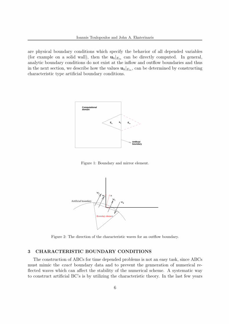
are physical boundary conditions which specify the behavior of all depended variables(for example on a solid wall), then the uh|Em can be directly computed. In general,analytic boundary conditions do not exist at the inflow and outflow boundaries and thusin the next section, we describe how the values uh|Em , can be determined by constructingcharacteristic type artificial boundary conditions.

Computationaldomain

Eb Emeb

Artificialboundary

Figure 1: Boundary and mirror element.

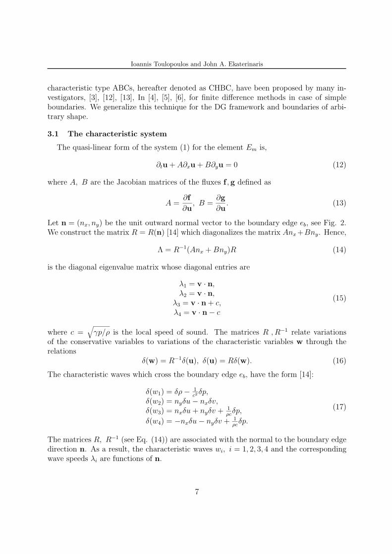
Boundary element

n

Artificial boundary ww1

4

w2w3

Figure 2: The direction of the characteristic waves for an outflow boundary.

3 CHARACTERISTIC BOUNDARY CONDITIONS

The construction of ABCs for time depended problems is not an easy task, since ABCsmust mimic the exact boundary data and to prevent the genneration of numerical re-flected waves which can affect the stability of the numerical scheme. A systematic wayto construct artificial BC’s is by utilizing the characteristic theory. In the last few years

6


characteristic type ABCs, hereafter denoted as CHBC, have been proposed by many in-vestigators, [3], [12], [13], In [4], [5], [6], for finite difference methods in case of simpleboundaries. We generalize this technique for the DG framework and boundaries of arbi-trary shape.

3.1 The characteristic system

The quasi-linear form of the system (1) for the element Em is,

∂tu + A∂xu + B∂yu = 0 (12)

where A, B are the Jacobian matrices of the fluxes f ,g defined as

A =∂f

∂u, B =

∂g

∂u. (13)

Let n = (nx, ny) be the unit outward normal vector to the boundary edge eb, see Fig. 2.We construct the matrix R = R(n) [14] which diagonalizes the matrix Anx +Bny. Hence,

Λ = R−1(Anx + Bny)R (14)

is the diagonal eigenvalue matrix whose diagonal entries are

λ1 = v · n,λ2 = v · n,

λ3 = v · n + c,λ4 = v · n− c

(15)

where c =√

γp/ρ is the local speed of sound. The matrices R ,R−1 relate variationsof the conservative variables to variations of the characteristic variables w through therelations

δ(w) = R−1δ(u), δ(u) = Rδ(w). (16)

The characteristic waves which cross the boundary edge eb, have the form [14]:

δ(w1) = δρ− 1c2

δp,δ(w2) = nyδu− nxδv,δ(w3) = nxδu + nyδv + 1

ρcδp,

δ(w4) = −nxδu− nyδv + 1ρc

δp.

(17)

The matrices R, R−1 (see Eq. (14)) are associated with the normal to the boundary edgedirection n. As a result, the characteristic waves wi, i = 1, 2, 3, 4 and the correspondingwave speeds λi are functions of n.

7


We multiply (12) by the matrix R−1 and after some algebra, we obtain the followinghyperbolic type system for the characteristic waves ,

(∂

∂t+ v · ∇)w1 = 0,

(∂

∂t+ v · ∇)w2 =

c

2(nx∂y − ny∂x)(w3 + w4),

(∂

∂t+ (v + cn) · ∇)w3 = c(nx∂y − ny∂x)w2, (18)

(∂

∂t+ (v − cn) · ∇)w4 = c(nx∂y − ny∂x)w2.

If Fw and Gw are the fluxes of the left and the right side of (18) respectively, then (18)can be written as

∂

∂tw + Fw = Gw. (19)

The right hand side of (19) expresses the variation of the waves along the tangentialto the boundary direction s = (ny,−nx). Following the approach applied for the inte-rior Riemann solver, where the normal to the interface flux is evaluated, the right-handside tangential flux Gw of the system (19) is neglected and the following evolution-typeequation for the time evaluation of the characteristic waves on Em is obtained:

∂tw + Fw = 0. (20)

The system (20) is referred to as the characteristic system, CHS.This system is solved numerically for all mirror elements of the artificial boundary, ac-cording to an upwind discretization in order to obtain a discrete approximation of thetime variation of the waves ∂t(w)|Em . Our goal is to relate this discrete time variation ofthe waves ∂t(wh) which cross the artificial boundary through edge eb as closely as possiblewith the corresponding discrete time variation of the conservative variable ∂t(uh|Em).

3.1.1 Discrete formulation of the CHS

For the element Em, the solution w of (20) is approximated, with the discontinuousGalerkin method by wh ∈ Vh(Em) such that,

∫Em

∂wh

∂tϕdxdy = − ∫

EmFw(wh)ϕdxdy+∫

ebΛ(uh|Eb

,uh|Em)R−1(uh|Eb,uh|Em)(uh|Eb

− uh|Em)ϕds, ∀ϕ ∈ Vh(Em)(21)

where Λ, R−1 are evaluated at the Roe’s average state on the midpoint of eb. Replacingin (21) the ϕ by the polynomial elements of the base of Vh(Em), we obtain a system ofODE’s for the degrees of freedom W of wh

dW

dt= LEm(wh) (22)

8


where the right side LEm results from the right hand side of (21) multiplied by the inversemass matrix M−1.

From (22) and (16), the following system for the time variation of the conservativevariables in Em is obtained

dU

dt= R

dW

dt= RLEm(wh) = Lbc(uh)|Em (23)

where R is computed at the Roe’ average state on midpoint of eb and U is the vector ofthe degrees of freedom of uh|Em , to be advanced in time.

The system (23) defines the ABCs (referred to as the ABC-ODE system) and is ad-vanced in time using the Runge-Kutta method (10). We note that for the numericalsolution of ABC-ODE by Runge-Kutta method, the characteristic waves (the right handside) at the intermediate stage l, l = 1, 2, 3, are computed using the solution data fromthe previous stage Un,l−1|Em , see (10). The numerical solution obtained from (23) yieldsvalues of the conservative state variable vector uh on the mirror element Em of the arti-ficial boundary. Using these values the numerical flux h(uh|Eb

,uh|Em), (see (11)), on eb

can be computed.

4 NUMERICAL EXAMPLES

The first problem is the propagation of a vortex in a uniform stream. Convection of avortex through an artificial outflow computational boundary is a difficult time-dependedtest problem. For this problem, boundary treatment procedures based on one-dimensionalRiemann invariant extrapolation, usually fails. For this case, the flow near the bound-ary cannot be represented as a small amplitude disturbance to a uniform state and anyartificial boundary treatment is not fully nonreflective. The convection of the isentropicvortex is governed by the Euler equations. For this problem it is found that the incomingnumerical waves do not strongly affect the overall accuracy of the numerical solution.Furthermore, the numerical perturbations generated by the incoming wave are not ableto destroy the stability of the method.

We used the same boundary conditions for the numerical solution of aeroacoustic prob-lems. The first problem of this category concerns the scattering of an acoustic pulse bya circular cylinder, [15], [16]. The second problem of this category has a time periodicsolution and is the propagation of acoustic pulses generated by a time harmonic source,[16].

In the numerical examples we denote the numerical solutions computed by the applica-tion of the proposed boundary treatment as CHBC. For certain problems where the exactsolution is known, we also obtained numerical solutions using boundary values specifiedby the exact solution. In these cases, the analytical specification of boundary data is usedfor comparison. We denote the corresponding numerical solutions as ExBc. The localpolynomial space for all the problems is Vh(E) = P3(E), ∀E ∈ Th.

9


4.0.2 Isentropic Vortex Convection

The DG finite element method, with the proposed characteristic boundary conditions,is used for the convection of a vortex through the computational boundary. The freestream flow velocity, pressure, and density are prescribed as:

[ρ∞, u∞, v∞, p∞] = [1, 1, 0, 1] .

The initial condition for the isentropic vortex is the addition of perturbations in thevelocity components (u, v) and temperature T (no perturbation in entropy) to the freestream. These perturbations are given by:

(δu, δv) = (β

2πe

1−r2

2 (−y′, x′)) (24)

δT = −(γ − 1)β2

8γπ2e1−r2

where β is the vortex strength, γ = 1.4, and (xvo, yvo) are the initial coordinates of thevortex center, (x′, y′) = (x − xv, y − yv), and r2 = x′2 + y′2. In the absence of viscousterms, the entire flow field is required to be isentropic, δS = 0, and the initial conditionfor the conservative state variables vector u(x, y, 0) = u0 is

u0 =

ρρuρvρe

=

(1 + δT )1

γ−1

ρ(u∞ + δu)ρ(v∞ + δv)p

γ−1+ ρ(u2+v2)

2

. (25)

The exact solution remains self similar for all times and represents a passive convectionof the vortex with the freestream velocity (u, v). In the numerical examples, β = 2. and(xvo, yvo) = (8., 0).

Fig. 3(a) shows the initial density field for discretization of the domain with ∆x = 0.5.The entire flow-field is mixed subsonic and supersonic

uc

< 1, for y > 0uc

> 1, for y < 0,

as it is shown in Fig.3(b). The numerical solution is computed on regular triangularmeshes using grid spacing ∆x = 0.5, 0.25, 0.125. Time iterations start and the vortex isconvected downstream. At computational time t = 2 the center of the vortex is locatedat the outflow boundary point (10,0), and half vortex has passed through the artificialboundary out of the computational domain. Fig. 4 shows the crossing of the vortexmoving with u∞ = 1 through the outflow boundary for the grid size ∆x = 0.125 att = 2. In Fig. 4(a) CHBC have been used and in Fig 4(b) the boundary values have

10


been specified by the analytic solution, ExBC. It is seen, Fig. 4(a), that the shape ofthe vortex of the supersonic part y < 0 has not changed, while the shape of the vortexcorresponding to the subsonic part y > 0 has been deformed.

The vortex continues to escape through the outflow boundary and for a later timet = 4 the vortex has moved out of the computational domain. However, Fig. 5 shows thatperturbations generated during the passage of the vortex through the outflow boundaryremain in the computational domain.

At time t = 4 the L2 error of the density variable

||ρh − ρexact||2 =

∑E∈Th

√∫E(ρh − ρexact)2

Nel

,

is computed for the three different grids. The convergence rate of the L2 error is shown inFig. 6. The dashed line shows the reduction of the L2 error using characteristic BC versus∆x. The dotted line shows the error reduction using exact (analytical) boundary dataspecified by the analytical solution, (ExBC). It is seen that the slope of the characteristicBC line is one order less than the corresponding slope of the ExBC line.

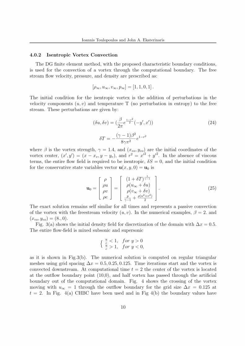
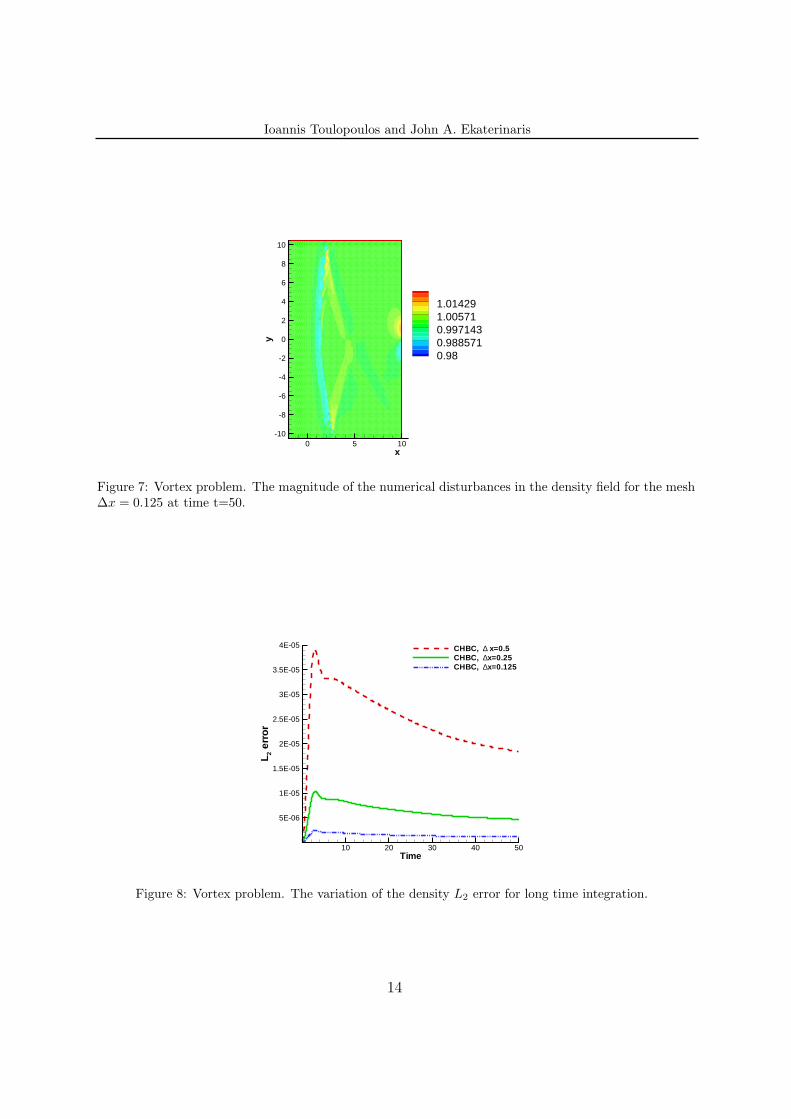
At later times the vortex has disappeared. However due to imperfections of the charac-teristic boundary conditions, spurious numerical waves which have been generated duringthe passage from the outflow boundary remain in the computational domain. These nu-merical waves propagate in the computational domain towards the inflow. The contoursof these numerical disturbances at time t = 50 are shown in Fig. 7 and have small mag-nitude, about 2% of the free stream density. The variations of the global L2 error versustime are shown in Fig. 8. It can be seen that the L2 error decreases with the meshrefinement, however even after long time integration the numerical computation remainsstable.

11

Ioannis Toulopoulos and John A. EkaterinarisIn

flow

BC

0 2 4 6 8 10-5

-4

-3

-2

-1

0

1

2

3

4

5

0.98710.96790.94860.92930.9100

Ou

tfowB

C

Free stream B C

Free stream B C

(a) Initial position of the vortex, density contours

xy

0 2 4 6 8 10-5

-4

-3

-2

-1

0

1

2

3

4

5

1.028570.9214290.8142860.7071430.6

u/c <1

u/c > 1

(b) Contours of u/c

Figure 3: Vortex propagation through a subsonic outflow boundary, ∆x = 0.5, t = 0.

x

y

5 6 7 8 9 10 11 12-3

-2

-1

0

1

2

3

0.9872290.9614860.9357430.91

(a) Subsonic outflow boundary, CHBC

y

-3

-2

-1

0

1

2

3

0.9872290.9679210.9486140.9293070.91

Analyticalb

oundary

data

(b) Subsonic outflow boundary, ExBC

Figure 4: Vortex crossing through the computational boundary: density contours computed on mesh∆x = 0.125 at t = 2. (a) Half vortex has crossed the subsonic outflow boundary using CHBC, (b) Halfvortex has crossed the subsonic outflow boundary using ExBC.

12


x

y

0 2 4 6 8 10 12 14-6

-4

-2

0

2

4

6

1.00570.99950.99280.98640.98

Figure 5: Remaining perturbations of density field on mesh ∆x = 0.125 at t = 4. The vortex has left thecomputational domain and spurious numerical waves generated by the crossing on the vertical boundary.

log(∆x)

log(

L 2)

erro

r

0.125 0.25 0.375 0.5

10-8

10-7

10-6

10-5

10-4

CH BCExBCSlope = 2.15

Slope = 3.14

Figure 6: Vortex problem. The convergence rate of the L2 error of the density, dashed line CHBC, dottedline ExBC.

13


x

y

0 5 10 15 20-10

-8

-6

-4

-2

0

2

4

6

8

10

1.014291.005710.9971430.9885710.98

Figure 7: Vortex problem. The magnitude of the numerical disturbances in the density field for the mesh∆x = 0.125 at time t=50.

Time

L 2er

ror

10 20 30 40 50

5E-06

1E-05

1.5E-05

2E-05

2.5E-05

3E-05

3.5E-05

4E-05 CHBC, ∆ x=0.5CHBC, ∆x=0.25CHBC, ∆x=0.125

Figure 8: Vortex problem. The variation of the density L2 error for long time integration.

14


4.1 Performance of CHBC for aeroacoustic problems

4.1.1 Scattering of an acoustic pulse by a cylinder surface

Scattering of an aeroacoustic pulse by the surface of a circular cylinder is considerednext. The center of the cylinder is (x, y) = 0.0 and its radius r = 0.5. The outflowboundary part of Ω is the hemicycle Γoutflow bd = (x, y) :

√x2 + y2 = 10, y ≥ 0.

The rigid boundary comprises the up half of the surface of the cylinder Γcyl = (x, y) :√x2 + y2 = 0.5, y ≥ 0 and the points (x, y),−10 ≤ x ≤ 0.5, y = 0⋃(x, y), 0.5 ≤

x ≤ 10, y = 0. The pulse is introduced by the initial pressure disturbance centered at(x, y) = (4, 0). The initial conditions are

u0 =

ρ0 = 1u0 = 0v0 = 0

p0 = ε exp(− ln(2)w

((x− 4)2 + y2))

where in our numerical experiments we set the Gaussian half-width w = 1 and ε = 0.01.Further details on the set up of this problem can be found in [15]. The computa-tional domain is divided in consequence of three triangular meshes using in every meshfiner discretization for both the Γoutflow bd and for the Γcyl. For the coarse mesh theΓoutflow bd, Γcyl are discretized by Noutflow bd = 6 elements. For the medium mesh thesurface are discretized using Noutflow bd = 12 and for the fine mesh using Noutflow bd = 24elements. We can approximately consider that the size of the Γoutflow bd discretization is

∆Γoutflow bd =Γoutflow bd

Noutflow bd. The problem for the three meshes is solved at final time t = 8.

The pressure field computed on the finer mesh (Noutflow bd = 24) is shown in Fig. 9,where the incident and scattered acoustic pulse leave the computational domain throughthe Γoutflow bd without the appearance of incoming numerical waves. For each of the threemeshes, we computed the LEb

2 error on the boundary elements of the outflow boundaryat t = 8. The grid converge of the LEb

2 error is presented in Fig. 10. The order of theconvergence is r = 2.97, which is close to the optimal order for the outflow surfaces isr = m + 1

2, [17], ( for our polynomial space r = 3 + 1

2).

4.1.2 The time harmonic source problem

The last aeroacoustic problem examined is the calculation of the perturbation pressurefield generated by a time dependent source. This problem provides a stringent case for thetest of the artificial BC because acoustic waves continuously cross the outflow boundary.The time depended acoustic source term has the form

S(x, y, t) = ε exp(− ln(2)

w((x− 4)2 + y2))sin(ωt)

and is added to the right-hand side of (1) for the energy equation. In the numericalexperiments we chose ε = 0.01, w = 1, ω = 0.5π.

15


x

y

-10 -5 0 5 100

5

10

15

0.715350.7151250.71490.7146750.714450.7142250.714

Pressure field

Figure 9: Acoustic pulse scattering problem. The final pressure field at T=8 computed on the fine meshusing the characteristic boundary conditions on the outflow boundary.

log(∆Γ) outflow boundary

log(

L 2Eb )

1 1.5 2 2.5 3 3.5 4 4.5

0.0002

0.0004

0.0006

0.0008

0.001

Slope=2.97

Figure 10: Acoustic pulse scattering problem. The converge rate of the LEb2 error at t = 8.

16


The outflow boundary computational domain is

Γoutflow bd = (x, y) : x = rcos(θ), y = rsin(θ), 0 ≤ θ ≤ 2π, r = 10.The computational domain is discretized in two triangular meshes, coarse and fine. Forthe first mesh the grid size on the outflow boundary is


40

and for the second mesh


80.

The problem has numerically solved at final time t = 350. The computed pressure fieldson the two meshes are shown in Fig. 11. For both meshes the pressure values are recordedat the point (x, y) = (10, 0) of the boundary. In Fig. 12(a) the numerical point valuescorresponding to the coarse mesh are compared with the exact pressure values. In Fig.12(b) we perform the same comparison for the numerical point values corresponding to thefine mesh. The LEb

2 error is computed on the elements of the boundary for both meshes.In Fig 13, the variations of the LEb

2 error versus time are presented. For both meshes thevalues of the LEb

2 error show periodic variation but remain bounded. Therefore it appearsthat the proposed characteristic BC approach is accurate and does not deteriorate thestability of the overall numerical scheme.

x

y

-10 -5 0 5 10-10

-8

-6

-4

-2

0

2

4

6

8

10

0.74900.74210.73520.72840.72150.71460.70770.70090.6940

(a)

x

y

-10 -5 0 5 10-10

-8

-6

-4

-2

0

2

4

6

8

10

0.74900.74210.73520.72840.72150.71460.70770.70090.6940

(b)

Figure 11: Acoustic time harmonic source problem. (a) The numerical pressure field computed at t = 350using CHBC on the coarse mesh. (b) The numerical pressure field computed at t = 350 using CHBC onthe fine mesh.

17


Time

Pre

ssur

eon

boun

dary

poin

t

50 100 150 200 250 300 3500.712

0.714

0.716

0.718Exact pressureCHBC

190 195 200 205 210

0.714

0.715

(a)

Time

Pre

ssur

eon

boun

dary

poin

t

50 100 150 200 250 300 3500.712

0.714

0.716

0.718Exact pressureCHBC

190 195 200 205 210

0.714

0.7145

(b)

Figure 12: Acoustic time harmonic source problem. (a) Coarse mesh. The exact and the numericalboundary point values of the pressure versus time. (b) Fine mesh. The exact and the numerical boundarypoint values of the pressure versus time.

Time

L 2Eb

50 100 150 200 250 300 350-0.0002

-0.0001

0

0.0001

0.0002

0.0003

0.0004CHBC fine meshCHBC coarse mesh

190 195 200 205 2100

2E-05

4E-05

6E-05

8E-05

0.0001

0.00012

Figure 13: Acoustic time harmonic source problem. The time variation of the LEb2 error for the two

meshes.

18


5 CONCLUSIONS

Artificial boundary conditions based on the characteristic analysis of the Euler’s equa-tions were developed and applied in the DG framework. These boundary conditions areapplicable to artificial boundaries with arbitrary shape. An auxiliary system was con-structed through application of characteristic analysis. The numerical solution of thissystem is used for the evaluation of the time variation of the characteristic waves whichcross the artificial boundary. The time variation of these waves was related to the con-servative variables time variation resulting in an ODE system. The numerical solutionof this system mimics adequately the analytical boundary data. Computed results withthe proposed boundary conditions demonstrated that complex flow features can be con-vected outside the computational domain with little distortion. In addition, propagationof small amplitude acoustic-type perturbations with the proposed boundary conditionsdemonstrated equally good performance with exact boundary data.

REFERENCES

[1] Toulopoulos I. and Ekaterinaris J. Artificial boundary conditions for the numericalsolution of the euler equations by the discontinuous galerkin method. Under review,2009.

[2] D. Givoli. Non-reflecting boundary conditions. Journal of Computational Physics,91:1–29, 1991.

[3] T Colonious. Modeling artificial boundary conditions for compressible flow. AnnualReview of Fluid Mechanics, 36:315–345, 2004.

[4] K. W. Thompson. Time dependent boundary conditions for hyperbolic systems.Journal of Computational Physics, 68:1–24, 1987.

[5] K. W. Thompson. Time-dependent boundary conditions for hyperbolic systems,ii.Journal of Computational Physics, 89:439–461, 1990.

[6] T.J. Poinsot and S.K. Lele. Boundary conditions for direct simulations of compress-ible viscous flows. Journal of Computational Physics, 101:104–129, 1992.

[7] L. Selle, F. Nicoud, and T. Poinsot. Actual impedance of nonreflective boundaryconditions: Implications for computation of resonators. AIAA Journal, 42(5):958–964, 2004.

[8] T. Colonious, S. K. Lele, and P. Moin. Boundary conditions for direct computationof aerodynamic sound generation. AIAA Journal, 31(9):1574–1582, 1993.

[9] T Colonious. Numerical nonreflecting boundary and interface conditions for com-pressible flow and aeroacoustic computations. AIAA Journal, 35(7):1126–113, 1997.

19


[10] Jianxian Qiu, Boo Cheong Khoo, and Chi Wang Shu. A numerical study for theperformance of the runge-kutta discontinuous Galerkin method based on differentnumerical fluxes. Journal of Computational Physics, 212(2):540–565, 2006.

[11] B Cockburn and C.W. Shu. The runge-kutta discontinuous galerkin method forconservation laws, multidimensional systems. Journal of Computational Physics,141:199–224, 1998.

[12] M Giles. Nonreflecting boundary conditions for euler calculations. AIAA Journal,28:2050–2058, 1990.

[13] G. W. Hedstrom. Nonreflective boundary conditions for the nonlinear hyperbolicsystems. Journal of Computational Physics, 30:222–237, 1979.

[14] C. Hirsch. Numerical Computation of Internal and External Flows, volume 2, Compu-tational methods for inviscid and viscous flows of Wiley series in numerical methodsin engineering. Wiley, 1988.

[15] I. Toulopoulos and J. A. Ekaterinaris. High-order discontinuous-galerkin discretiza-tions for for computational aeroacoustics in complex domains. AIAA Journal,44(3):502–511, 2006.

[16] J. C. Hardin, J. R. Ristorcelli, and C. K. Tam. Icase/larc workshop on benchmarkproblems in computational aeroacoustics (caa), nasa cp 3300. 1995.

[17] P. Monk and G. R Richter. A Discontinuous Galerkin Method for Linear SymetricHyperbolic Systems in Inhomogeneous Media. Journal of Scientific Computing, 22-23:443–477, 2005.

20

characteristic boundary conditions for the … · j. c. f. pereira and a. sequeira (eds) lisbon,...

Documents