characteristics of thz carrier dynamics...
TRANSCRIPT
CHARACTERISTICS OF THZ CARRIER DYNAMICS
IN GaN THIN FILM AND ZnO NANOWIRES BY TEMPERATURE DEPENDENT
TERAHERTZ TIME DOMAIN SPECTROSCOPY MEASUREMENT
by
SONER BALCI
SEONGSIN MARGARET KIM, COMMITTEE CHAIR
PATRICK KUNG
DANIEL J. GOEBBERT
A THESIS
Submitted in partial fulfillment of the requirements
for the degree of Master of Science
in the Department of Electrical and Computer Engineering
in the Graduate School of
The University of Alabama
TUSCALOOSA, ALABAMA
2012

Copyright Soner Balci 2012
ALL RIGHTS RESERVED

ii
ABSTRACT
We present a comprehensive study of the characteristics of carrier dynamics using
temperature dependent Terahertz Time Domain Spectroscopy. By utilizing this technique in
combination with numerical calculations, the complex refractive index, dielectric function, and
conductivity of n-GaN, undoped ZnO NWs, and Al-doped ZnO NWs were obtained. The unique
temperature dependent behaviors of major material parameters were studied at THz frequencies,
including plasma frequency, relaxation time, carrier concentration and mobility. Frequency and
temperature dependent carrier dynamics were subsequently analyzed in these materials through
the use of the Drude and the Drude-Smith models.

iii
ACKNOWLEDGMENTS
I would like to thank my advisors, Dr. Seongsin Margaret Kim and Dr. Patrick Kung for
all of their support, guidance, and patience during my graduate study. I also wish to thank Dr.
Daniel J. Goebbert for his time, support of my work, and willingness to serve on my thesis
committee. Additionally, I would like to thank my colleagues, Shawn and Eli, for the
experimental part, and Gang, for the materials growth part of this work.
iv
CONTENTS
ABSTRACT ................................................................................................ ii
ACKNOWLEDGMENTS ......................................................................... iii
LIST OF TABLES ..................................................................................... vi
LIST OF FIGURES .................................................................................. vii
1. INTRODUCTION ...................................................................................1
2. BACKGROUND .....................................................................................5
2.1 THz Time Domain Spectroscopy...........................................................5
2.2 Theoretical Background of the Data Analysis .......................................7
3. SIMULATION METHOD.....................................................................12
3.1 Array of Complex Refractive Index Values ........................................13
3.2 Calculation of With Array n ..............................................................15
3.3 Error Function and Refractive Index ...................................................15
3.4 Conductivity and Fitting ......................................................................16
4. THz MEASUREMENTS .......................................................................19
4.1 Experimental Set-up.............................................................................19
4.2 Temperature Dependent THz-TDS Measurements .............................22
4.3 Fast Fourier Transform (FFT) ..............................................................23
5. GaN THIN FILM ...................................................................................26
5.1 Refractive Index ...................................................................................27
5.2 Conductivity and Fitting ......................................................................29
v
6. ZnO NANOWIRES ...............................................................................33
6.1 Undoped ZnO NWs .............................................................................34
6.1.1 Refractive Index ................................................................................36
6.1.2 Conductivity and Fitting ...................................................................38
6.2 Al-doped ZnO NWs .............................................................................40
6.2.1 Refractive Index ................................................................................41
6.2.2 Conductivity and Fitting ...................................................................51
6.2.3 Comparison Summary ......................................................................57
7. CONCLUSION ......................................................................................60
REFERENCES ..........................................................................................61
vi
LIST OF TABLES
5.1 Fitting Parameters for n-GaN ...............................................................32
6.1 Fitting Parameters for Undoped ZnO NWs at Room Temperature .....40
6.2 Doping Details of the Al Doped ZnO NWs .........................................41
6.3 Fitting Parameters for Al Doped ZnO NWs: Sample A ......................58
6.4 Fitting Parameters for Al Doped ZnO NWs: Sample B ......................58
6.5 Fitting Parameters for Al Doped ZnO NWs: Sample C ......................59
vii
LIST OF FIGURES
2.1 A chart that shows the wavelengths, energy, and frequency that
correspond to the THz radiation ..................................................................6
2.2 THz field transmitted through bare substrate which is Al2O3
(sapphire) in this study, ........................................................8
2.3 THz field transmitted through sample (GaN thin film or ZnO NWs)
and substrate (Al2O3 in this work), ...........................................9
3.1 The code simply generates the array of all possible complex values
for refractive index .....................................................................................14
3.2 A part of the code that calculates the transmission ratio with the
refractive index array .................................................................................15
4.1 Terahertz time domain spectrometer based on Ti:Sapp ultrafast laser
at 790nm.....................................................................................................20
4.2 (a) Basic THz signal waveform with full measurement cycle. (b) THz
signal waveform cleared of the echoes ......................................................21
4.3 The heating stage used in the temperature dependent THz
spectroscopy measurements .......................................................................22
4.4 Temperature stage calibration results ..................................................23
4.5 The magnitude of the fast Fourier transform of the finite length
discrete time signal shown in Figure 4.2(b) ...............................................25
5.1 SEM image of the GaN epilayer on sapphire substrate .......................26
5.2 (a) Measured THz responses transmitted through both the GaN and
substrate, (b) temperature dependent measurement of GaN ......................27
5.3 Refractive index of GaN determined by THz-TDS .............................28
5.4 Conductivity of GaN ............................................................................29

viii
5.5 Measured real part of conductivity vs. frequency at three selected
temperatures and fitted using the simple Drude model .............................30
5.6 Summary of the temperature dependent fitting parameters of GaN ....31
6.1 SEM image of the cross section of vertically aligned ZnO NWs ........33
6.2 (a) Measured THz signal transmitted through undoped ZnO NWs,
(b) Peak amplitudes vs. temperatures for undoped ZnO NWs ..................35
6.3 Real part of refractive index vs. frequency and temperature for
undoped NWs.............................................................................................37
6.4 Complex conductivity of undoped NWs at 25oC .................................38
6.5 Real conductivity and curve fit (at 25oC) using the Drude-Smith
model for undoped NWs at different temperatures....................................39
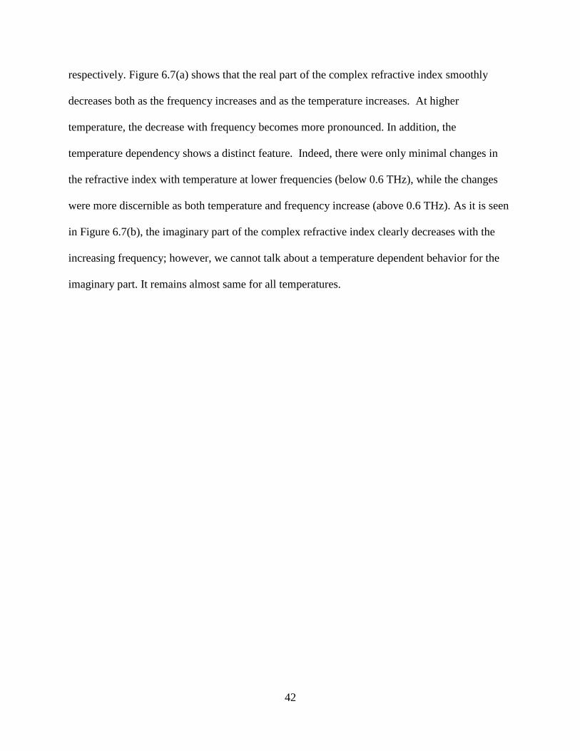
6.6 (a) THz signal transmitted through Sample A, (b) Peak amplitudes vs.
temperatures for Sample A ........................................................................43
6.7 Refractive index vs. frequency and temperature for Sample A ...........44
6.8 (a) THz signal transmitted through Sample B, (b) Peak amplitudes vs.
temperatures for Sample B.........................................................................46
6.9 Refractive index vs. frequency and temperature for Sample B ...........47
6.10 (a) THz signal transmitted through Sample C, (b) Peak amplitudes
vs. temperatures for Sample C ...................................................................49
6.11 Refractive index vs. frequency and temperature for Sample C .........50
6.12 Conductivity of Sample A at 25oC.....................................................51
6.13 Conductivity and curve fits for Sample A .........................................52
6.14 Conductivity of Sample B at 25oC .....................................................53
6.15 Conductivity and curve fits for Sample B..........................................54
6.16 Conductivity of Sample C at 25oC .....................................................55
6.17 Conductivity and curve fits for Sample C..........................................56
6.18 Comparison of the peak amplitudes of all ZnO NWs samples .........57

ix

1
CHAPTER 1
INTRODUCTION
Terahertz time domain spectroscopy (THz-TDS) has been widely investigated for many
applications in sensing and imaging technologies over the past two decades. Terahertz wave,
with a frequency between 300GHz to 10THz, is especially attractive for various applications
including security monitoring, biomedical imaging, high speed electronics and communications,
and chemical and biological sensing. There is also an increasing interest for nondestructive
testing using the THz waves because they have unique properties of propagation through certain
media and cover a number of important frequencies. For such applications, THz-TDS has
become a powerful tool and measurement technique that enables carrier dynamics at high
frequencies to be characterized, and thus may lead to a better understand of the characteristics of
high frequency optoelectronics and many other fundamental properties of materials. [1-5]
Using THz-TDS, one can determine frequency dependent basic properties of any
material, including their complex dielectric constant, refractive index and electrical conductivity.
Unlike conventional Fourier-Transform spectroscopy, THz-TDS is sensitive to both the
amplitude and the phase, thereby allowing for a direct approach to determining complex values
of material parameters with the advantage of high signal to noise ratio and coherent detection [6].
In addition, it is possible to carry out THz-TDS experiments without any electrical contact to the
sample probed, which significantly simplifies electrical measurements of any type of
nanostructures and nanomaterials. There have been a number of works done on dielectric
properties of various materials probed by THz-TDS [7-9]. Among them, wide band gap GaN and

2
ZnO nanostructures are the most interesting materials to pursue because of their extensive
applications in optoelectronic devices, photovoltaics, and high frequency electronics devices [10-
14]. The high mobility and saturation drift velocity of GaN make it a good candidate for a high-
frequency transistor that can potentially operate beyond the gigahertz and reach to the terahertz
frequency range [15-17]. ZnO nanowires (NWs) have been intensively used for many different
types of sensors and recently for base structure for nanowire based photovoltaics [18]. For solar
cell applications, it is critical to know the electrical properties of such nanowires as they would
transport photogenerated carriers.
However, there has been no report of the temperature dependent behavior of material
properties probed at THz frequencies. Since temperature is an important factor in the operating
conditions of any device, understanding its effect on carrier dynamics in constituent materials is
a critical step in the optimization of high-frequency devices. In this work, we present a study of
the temperature dependent carrier dynamics in GaN thin films and ZnO NWs obtained from
THz-TDS measurements and extract important material properties in the THz frequency region.
This text is organized as follows:
Chapter 2 gives a brief background of THz frequency region; what it really is, what the
specialty about this region is. How does a THz time domain spectroscopy work? Why is it really
important? These questions are answered in Chapter 2, as well. There will also be an explanation
how the mathematical expression of the transmission ratio in terms of the complex refractive
indices is derived.
The simulation method used to determine the frequency dependent complex refractive
index by using the complex transmission ratio is discussed in Chapter 3. Calculation of complex
3
conductivity and fitting of this conductivity are mentioned in this chapter, as well. Some details
will be given such as the MATLAB code used for determination of the complex refractive index
and also for the fitting process of the conductivity.
In Chapter 4, the THz time domain spectroscopy measurement is explained. The
experimental set-up is overviewed including the system limitation. There will be some examples
of general THz signals in time domain, basic waveforms, and as well as the Fourier transformed
THz signals. To compute the Fourier transform of a discrete signal such as the THz signals
measured in this work, an efficient algorithm called Fast Fourier Transform (FFT) is used. The
basic idea of FFT is also covered in this chapter. At last, the temperature dependent
measurement, which is the main goal of this work, is explained, as well as the additional tools
used to achieve this measurement.
One of the wide band gap materials used in this work is GaN. Why GaN was choosen is
discussed in Chapter 5. The sample details such as the thickness and the hall measurement will
be presented. By using the mathematical expressions discussed in Chapter 2, the frequency
dependent refractive index is determined through numerical iteration process and presented in
this chapter. Once the index of refraction is known, the complex conductivity is calculated
directly. Then, by fitting the calculated conductivity with the appropriate Drude model, some
important material parameters of GaN thin film is obtained.
Chapter 6 is about the ZnO NW samples used in this study. We basically have two
different kinds of ZnO NW samples: undoped and Al doped ZnO NWs. While we have one
undoped ZnO NW sample, we used three Al doped ZnO NW samples with different doping
ratios. The details about the differences in the samples such as doping ratios and thicknesses are
4
also presented in this chapter. Applying the same numerical iteration method that was used for
GaN thin film in Chapter 5, the complex index of refraction is determined for all undoped and Al
doped ZnO NW samples. Then, the frequency dependent complex conductivities are calculated
for each sample by using the corresponding refractive indices. For fitting process, another type of
Drude model, which is different than the one used for GaN thin film conductivity, is chosen
according to the different behaviour of the ZnO NW conductivity.
Chapter 7 gives a short summary of the results obtained during this work.

5
CHAPTER 2
BACKGROUND
In this chapter, detailed background information of THz frequency region, THz time
domain spectroscopy (THz-TDS), and data analysis in THZ-TDS are given. The importance and
specialty of THz radiation is explained. For the data analysis, a mathematical expression is
derived from which the frequency dependent complex refractive index can be determined
through numerical iteration process.
2.1 THz Time Domain Spectroscopy
The wavelengths which lie between 30μm and 1 mm can be called as THz radiation or
THz spectral region. Figure 2.1 would be a good chart to visualize where this frequency region
stands between other known frequency regions. As it is also expressed in Figure 2.1, the
frequency and energy are proportional to each other, unlike wavelength. We can say the terahertz
radiation has higher frequency and energy but lower wavelength than the radio frequency and
microwave, while it has higher wavelength but lower frequency and energy than the X-ray and
gamma ray. So far, it has not clearly been understood how the materials interact with each other
in terahertz frequency region. One of the main reasons why researchers have a huge interest in
THz spectral region is that the THz radiation can be transmitted through various organic
materials without giving any harm caused by ionizing radiation; especially it is safe for
biological tissues. Various interesting materials can be detected with the help of the unique

6
signals transmitted through each one. Since water is a good absorber of THz waves, THz
radiation can also be used to figure out how much water the materials contain.
Figure 2.1 A chart that shows the wavelengths, energy, and frequency that correspond to
the THz radiation.
An object which absorbs all electromagnetic radiations at any frequency is called a black
body. When a black body is at a constant temperature, it begins to radiate, called black-body
radiation. By this phenomenon, anything at a temperature higher than 10 K can be the source of a
terahertz radiation. However this radiation would be very weak. Therefore, various sources were

7
developed to generate terahertz radiation such as the gyrotron, far-infrared lasers, quantum
cascade laser, etc… Another source of THz radiation is photoconductive emitters which are also
used in terahertz time domain spectrometer (THz-TDS) used in this work.
THz time domain spectroscopy is one the most powerful tools to study material
properties in terahertz frequency range. THz-TDS uses short terahertz pulses with sub-
picosecond width. The spectrometer has two main components: a THz emitter and a THz
detector. A femtosecond laser system is used to pump the spectrometer: both emitter and the
detector.
2.2 Theoretical Background of the Data Analysis
To start data analysis, first we should define a THz pulse which is generated by the
THz-TDS system as the incident wave (emitted by the transmitted antenna). Analyzing the data
would be more convenient in frequency domain instead of time domain. Hence, let’s introduce
as Fourier transform of the time domain THz signal . (The details of Fourier transform
can be found in Chapter 4).
The complex reflection and transmission coefficients at the interface
( ) are defined as: and
, respectively. The propagation coefficient in medium over a distance
is defined as .
We consider the sample is homogeneous parallel plate with thickness (see Figure 2.3).
The complex spectral representation of the electric field of the THz wave transmitted through
bare substrate (see Figure 2.2) is given by
8
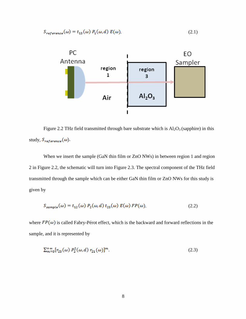
. (2.1)
Figure 2.2 THz field transmitted through bare substrate which is Al2O3 (sapphire) in this
study,
When we insert the sample (GaN thin film or ZnO NWs) in between region 1 and region
2 in Figure 2.2, the schematic will turn into Figure 2.3. The spectral component of the THz field
transmitted through the sample which can be either GaN thin film or ZnO NWs for this study is
given by
. (2.2)
where is called Fabry-Pérot effect, which is the backward and forward reflections in the
sample, and it is represented by
. (2.3)
9
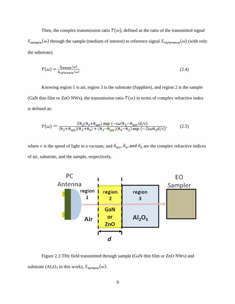
Then, the complex transmission ratio , defined as the ratio of the transmitted signal
through the sample (medium of interest) to reference signal (with only
the substrate).
(2.4)
Knowing region 1 is air, region 3 is the substrate (Sapphire), and region 2 is the sample
(GaN thin film or ZnO NWs), the transmission ratio in terms of complex refractive index
is defined as:
. (2.5)
where is the speed of light in a vacuum, and are the complex refractive indices
of air, substrate, and the sample, respectively.
Figure 2.3 THz field transmitted through sample (GaN thin film or ZnO NWs) and
substrate (Al2O3 in this work),
10
After going through a numerical iteration process -which is explained in the next chapter-
by using Equation (2.5) for the substrate, we figured out that the refractive index of Al2O3 does
not really change with frequency and does not have a strong imaginary part. Therefore, we
assumed the refractive index of the sapphire substrate is a real constant value.
One can have some assumptions in order to simplify the mathematical expression
depending on what kind of sample is used. For instance, if the sample measured by THz-TDS is
a thin film, i.e. 1, then the implicit complex transmission ratio will become
simpler and explicit:
(2.6)
To calculate the complex refractive index from the Equation (2.6), no numerical
iteration is needed anymore since the transmission ratio is now explicit. Just a simple
calculation is enough to determine the complex refractive index of the sample in Equation (2.6).
Another possible assumption to simplify the transmission ratio is having an
optically thick sample. In this case, we assume the sample is so thick that the backward and
forward reflections in the sample and the resultant echoes of the terahertz pulse are negligible.
Therefore, we don’t need to worry about the Fabry-Pérot effect (Equation (2.3)) anymore. Then,
in Equation (2.2). Consequently, the transmission ratio simplifies to:
(2.7)

11
However, since the mathematical expression for the transmission ratio in Equation (2.7)
is still implicit, numerical iteration should be applied to determine the complex refractive index
of the sample, which is discussed in Chapter 3.

12
CHAPTER 3
SIMULATION METHOD
In the previous chapter, we defined some mathematical expressions for some physical
concepts such as complex reflection and transmission coefficients at an interface and the
propagation coefficient in a medium. Using those expressions and making some assumptions,
finally we derived a complex transmission ratio in terms of the complex refractive index of the
sample we are interested in (Equation 2.5). It would be an easy calculation if we had an explicit
equation for the complex transmission ratio . However, we have to go through a numerical
iteration process in order to determine the complex index of refraction since the ratio is
totally implicit. For this purpose, an array that consists of all possible values of complex
refractive index is needed to be created.
We already have the complex transmission ratio calculated with the measured
signals (Equation (2.4)). What we need is to calculate the same transmission ratio with the array
created for possible refractive index values by using Equation (2.5). After that, the difference
between these two complex transmission ratios is calculated. Then, an error function is defined
to determine which element of the array makes this difference converge to zero. That element is
told to be the desired complex refractive index value. This process is repeated for each frequency
point.
Once index of refraction is determined, it is straight forward to calculate the frequency
dependent complex conductivity. The complex dielectric function is directly related with the
13
complex refractive index, and the conductivity is directly related with the dielectric function.
Obtaining complex conductivity, we can move on fitting process in order to extract some
important material parameters. How the fitting process is achieved for both GaN and ZnO
samples is explained in this chapter.
3.1 Array of Complex Refractive Index Values
Since the complex transmission ratio is an implicit function of the refractive index of the
sample in Equation (2.5), we sure need to consider numerical iteration. The index of
refraction we want to determine does not have to be pure real. We should give it a room to be a
complex value, as well. Therefore, the values plugged into Equation (2.5) should consist of both
real and imaginary components, defined as . To prevent process time to be
unnecessarily long, some limitations for both real and imaginary values can be defined such that
minimum values are 1 and 0, and the maximum values are 8 and 7 for real and imaginary parts,
respectively. The increment of 0.01 would be precise enough for this work. Even though there is
a limitation for the highest and lowest values, the total number of possible values is almost
500,000. It means Equation (2.5) is calculated for about 500,000 times (for each frequency point)
with one of the possible complex refractive index values each time. Each number could be
plugged into the equation one at a time in a for-loop. Then it would take 15-20 minutes for each
frequency point, and we have 50-70 frequency points depending on the case. Therefore, not to
have a process time about one day, we decided to create an array consisting of all possible values
of complex refractive index within the range defined above. The idea is to plug that array into
Equation (2.5) and calculate it one time instead of calculating one element at a time. To be able
to use matrices in our calculation, we preferred to use MATLAB since it gives us the freedom of
creating, manipulating, and calculating matrices. The following code (see Figure 3.1) is run one
14
time, and the resultant array is saved to be used later in another code to determine the refractive
index of the sample.
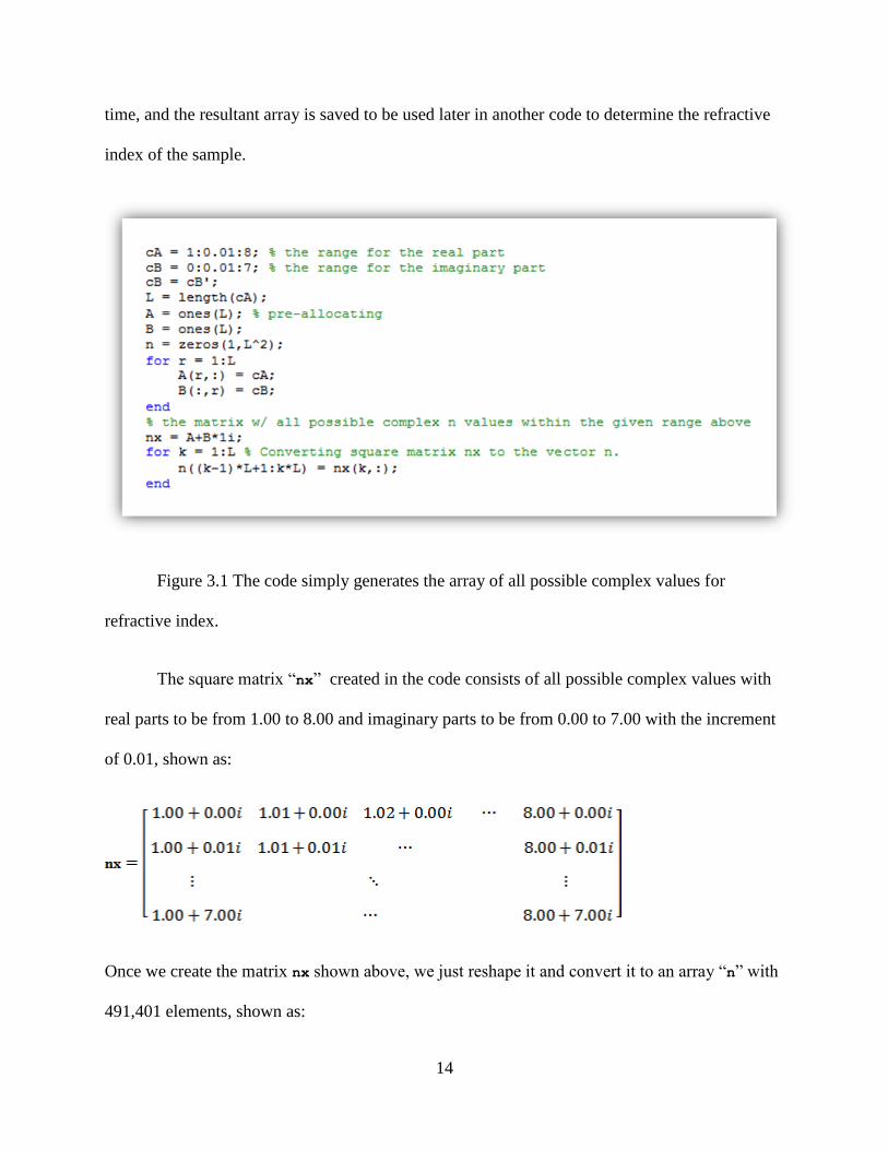
Figure 3.1 The code simply generates the array of all possible complex values for
refractive index.
The square matrix “nx” created in the code consists of all possible complex values with
real parts to be from 1.00 to 8.00 and imaginary parts to be from 0.00 to 7.00 with the increment
of 0.01, shown as:
Once we create the matrix nx shown above, we just reshape it and convert it to an array “n” with
491,401 elements, shown as:
15
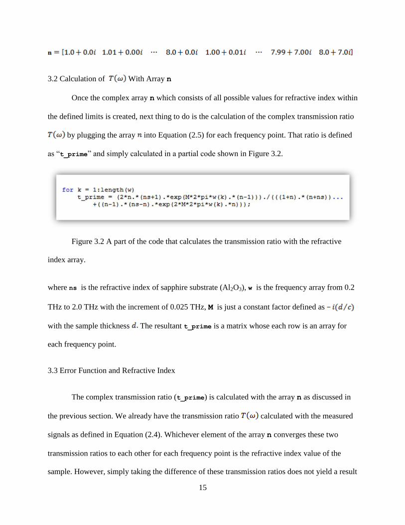
3.2 Calculation of With Array n
Once the complex array n which consists of all possible values for refractive index within
the defined limits is created, next thing to do is the calculation of the complex transmission ratio
by plugging the array into Equation (2.5) for each frequency point. That ratio is defined
as “t_prime” and simply calculated in a partial code shown in Figure 3.2.
Figure 3.2 A part of the code that calculates the transmission ratio with the refractive
index array.
where ns is the refractive index of sapphire substrate (Al2O3), w is the frequency array from 0.2
THz to 2.0 THz with the increment of 0.025 THz, M is just a constant factor defined as
with the sample thickness The resultant t_prime is a matrix whose each row is an array for
each frequency point.
3.3 Error Function and Refractive Index
The complex transmission ratio (t_prime) is calculated with the array n as discussed in
the previous section. We already have the transmission ratio calculated with the measured
signals as defined in Equation (2.4). Whichever element of the array n converges these two
transmission ratios to each other for each frequency point is the refractive index value of the
sample. However, simply taking the difference of these transmission ratios does not yield a result

16
successful enough since these two ratios are complex numbers. Therefore, an error function can
be defined having two components, one is about the magnitudes, and the other one is about the
arguments of the complex transmission ratios [24]. The first component is a function of the
logarithm of the magnitudes of the complex transmission ratios, defined as
(3.1)
and the second component is a function of the arguments of the complex ratios, defined as
(3.2)
where argument can also be called “phase angle” and defined as , and
magnitude is defined as with . Contribution
of Equation (3.1) and (3.2), the error function can be finalized as
(3.3)
Since the resultant error function is an array of pure real numbers for each frequency
point, we just look for the minimum value of the error function array, which leads us to the
desired complex refractive index value at each frequency point.
3.4 Conductivity and Fitting
After the complex refractive index of the sample is determined as a function of
frequency, the next thing to do is to calculate the complex conductivity. The dielectric function is
related with the complex index of refraction, defined as
(3.4)
17
Once the complex dielectric function is obtained, we can easily calculate the complex
conductivity by using the following relation between conductivity and dielectric function.
(3.5)
with the free-space permittivity , and a dielectric constant
for GaN and for ZnO.
Now, we know the frequency dependent complex index of refraction and conductivity.
Further, calculated conductivity is fitted with the appropriate Drude model for GaN and ZnO
samples.
For the fitting process of the conductivity of the GaN thin film, the proper model is
simple Drude model which has two parameters to be extracted: plasma frequency and the
characteristic relaxation time . Setting the upper and lower limits for both and , a row and
a column array are created for each of them. Plugging them into the simple Drude model as
arrays by using MATLAB, we obtain a 2D-array (matrix) for each frequency point consisting of
all possible complex conductivity values calculated with all possible and values within the
defined range. In each row and column, one of the variables ( , is not changing while the
other one is varying from lower limit to the upper limit with an increment defined before. By this
way, one matrix covers all possible values of complex conductivity calculated with possible
and values within the limits at each frequency point. Since this calculation is repeated for each
frequency point, the final yield is a 3D-array whose each flat (2D array) corresponds to one
frequency point. We already have the conductivity value calculated from the refractive index.
Subtracting the conductivity value at each frequency from the conductivity value matrix for the
18
corresponding frequency, we obtain a matrix of the differences. Since the fitting is processed in
least-squares sense, each element of the difference matrices is squared, and all corresponding
elements of each squared difference matrices are added to each other. What we have finally is a
matrix of added squared differences. Once we find the minimum value of this final matrix, by
knowing the corresponding row and column numbers, we can determine the fitting
parameters , and .
However, the frequency behavior of the conductivity of ZnO NW samples is different
than the one of GaN thin film. To fit the conductivity of the ZnO NW samples, the Drude-Smith
model is the appropriate one. In this model, there is an extra parameter compared with the simple
Drude model: a persistence of velocity parameter to describe the back scattering event. The
conductivity should be calculated with all possible values of the parameters , , and .
Having three fitting parameters in this case leads the calculated conductivity array to be four
dimensional: one dimension for plasma frequency , one for relaxation time , one for
parameter , and another one for the frequency , totally a 4D array. Since it would be kind of
complicated and time-consuming to run our own code, we preferred to use a built-in function
lsqcurvefit which also solves non-linear least squares problems.

19
CHAPTER 4
THz MEASUREMENTS
To be able to analyze the materials by using computational methods, first THz time
domain spectroscopy (THz-TDS) measurements should be done. In this chapter, how we
achieved THz-TDS measurements is explained. The experimental set-up used for this work and
the limitation of the instruments are also discussed. The most important part of this work,
temperature dependent THz-TDS measurement, is performed at elevated temperatures above
room temperature. For this part of the experiment, an extra component is added to the main
experimental set-up. Once all measurements are accomplished, Fast Fourier Transform (FFT) is
applied to the measured time domain THz signals before going through the computational
process.
4.1 Experimental Set-up
Terahertz measurements of the samples were carried out using the time-domain
transmission spectrometer shown in the Figure 4.1. A 790 nm mode-locked laser with 120 fs
pulses is used to pump the spectrometer. Broadband terahertz radiation (0.2-3.5 THz) is
generated by photo excitation of a photoconductive antenna based on LT-GaAs with an applied
voltage bias of 130 V at 15 kHz. Detection of the terahertz electric field is obtained using a
ZnTe electro-optic crystal and balanced photodiodes. The sample is mounted on a three-axis,
motion controlled stage perpendicular to the incident wave. Two polyethylene lenses are used to
20
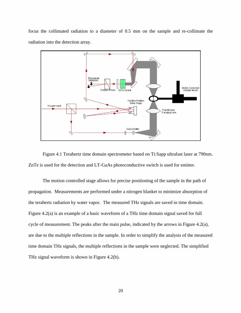
focus the collimated radiation to a diameter of 0.5 mm on the sample and re-collimate the
radiation into the detection array.
Figure 4.1 Terahertz time domain spectrometer based on Ti:Sapp ultrafast laser at 790nm.
ZnTe is used for the detection and LT-GaAs photoconductive switch is used for emitter.
The motion controlled stage allows for precise positioning of the sample in the path of
propagation. Measurements are performed under a nitrogen blanket to minimize absorption of
the terahertz radiation by water vapor. The measured THz signals are saved in time domain.
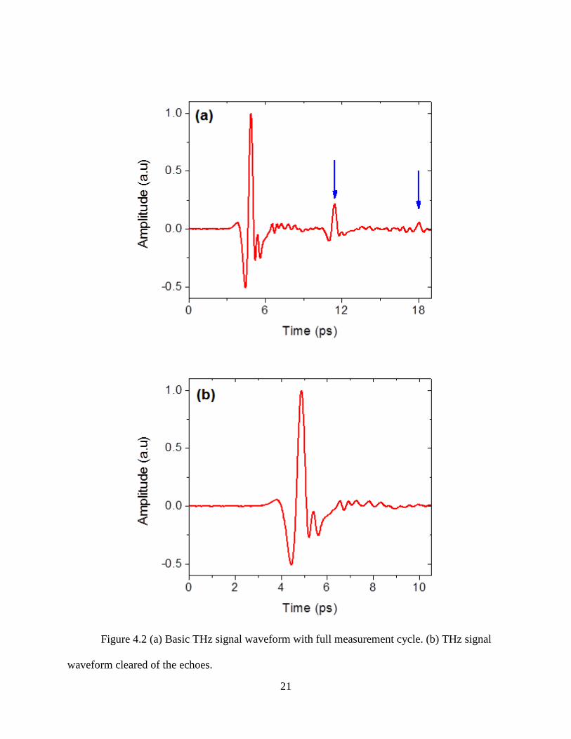
Figure 4.2(a) is an example of a basic waveform of a THz time domain signal saved for full
cycle of measurement. The peaks after the main pulse, indicated by the arrows in Figure 4.2(a),
are due to the multiple reflections in the sample. In order to simplify the analysis of the measured
time domain THz signals, the multiple reflections in the sample were neglected. The simplified
THz signal waveform is shown in Figure 4.2(b).
21
Figure 4.2 (a) Basic THz signal waveform with full measurement cycle. (b) THz signal
waveform cleared of the echoes.

22
4.2 Temperature Dependent THz-TDS Measurements
For the temperature dependent measurements, a mount with embedded resistance heating
was used, and the samples were placed in thermal contact in between two heated ceramic plates
with concentric 2 mm apertures, shown in Figure 4.3. The temperature of the mount is measured
by an embedded thermocouple and controlled using a basic feedback loop.
Figure 4.3 The heating stage used in the temperature dependent THz spectroscopy
measurements
The actual sample temperature is calibrated using an external thermocouple in contact
with the sample surface as a function of heating time and the embedded thermocouple. Careful
assessment of temperature and thermal stabilities were made for each step of increases and
decreases of the temperature as shown in Figure 4.4.

23
Figure 4.4 Temperature stage calibration results. It shows the thermal stability of each
step of increases and decreases of temperature as time passes.
4.3 Fast Fourier Transform (FFT)
Fourier Transform is used to transform a time domain signal (a function of time) as a
frequency domain signal (a function of frequency). The resultant frequency domain signal is also
called frequency spectrum for the time domain signal. The Fourier transform used to obtain the
spectral representation of a continuous-time signal is called the Continuous-Time Fourier
Transform, defined as
(4.1)
However, when the signal in interest is a function of discrete time and has a finite
sequence, then the Continuous-Time Fourier Transform sufficient to obtain the frequency
spectrum. Since the measurements performed for this study are based on sampling, which leads
the measured signal to be discrete in time, and the transmitted signals are measured for a finite
length of time, the Discrete Fourier Transform (DFT) would be the appropriate method to obtain
24
the spectral representation of the signals measured in this study. The Discrete Fourier Transform
is defined as
(4.2)
where is the total number of samples during the measurement, and is the amplitude of the
received signal at each sampling. We can say that DFT is the key to get the frequency spectrum
of a finite length discrete time signal. For computation speed concern, the fast Fourier transform
(FFT) was developed which is basically a discrete Fourier transform algorithm. By FFT, the
number of computations needed points is reduced from to . The idea is
basically splitting the DFT of -length signal into two transforms of -length signals,
defined as
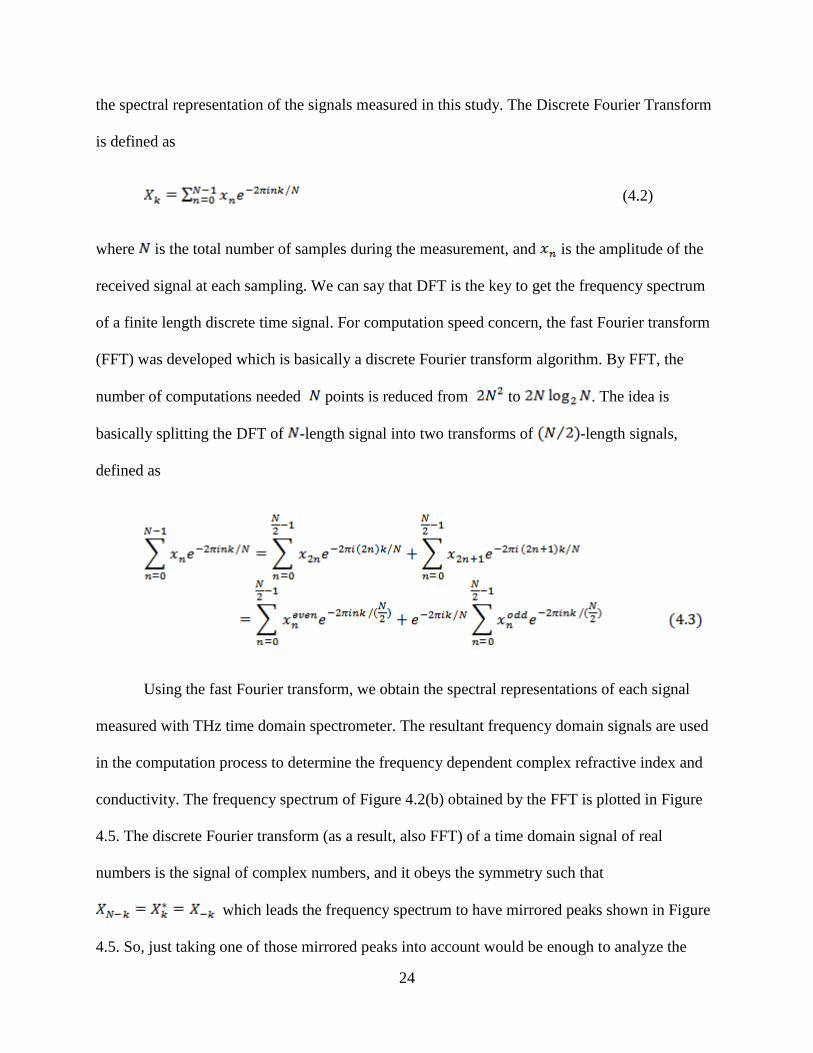
Using the fast Fourier transform, we obtain the spectral representations of each signal
measured with THz time domain spectrometer. The resultant frequency domain signals are used
in the computation process to determine the frequency dependent complex refractive index and
conductivity. The frequency spectrum of Figure 4.2(b) obtained by the FFT is plotted in Figure
4.5. The discrete Fourier transform (as a result, also FFT) of a time domain signal of real
numbers is the signal of complex numbers, and it obeys the symmetry such that
which leads the frequency spectrum to have mirrored peaks shown in Figure
4.5. So, just taking one of those mirrored peaks into account would be enough to analyze the
25
frequency spectrum. Analyzing the spectral representation in Figure 4.5, we can have an idea
about the contribution of each frequency. What Figure 4.5 tells us is we do not need to take into
account the frequencies much higher than ~2.0 THz. Therefore, we can say the limit of the THz
time domain spectrometer used in this work is about 2.0 THz.
-4 -2 0 2 40.0
0.5
1.0
Ma
gn
itu
de
(a
.u)
Frequency (THz)
Figure 4.5 The magnitude of the fast Fourier transform of the finite length discrete time
signal shown in Figure 4.2(b).
26
CHAPTER 5
GaN THIN FILM
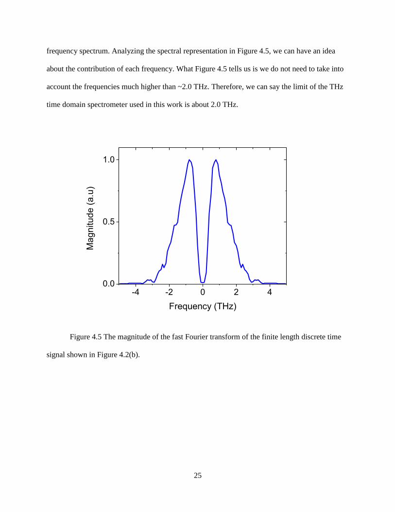
The GaN thin film used in this study is 4.8 μm thick, n-type doped and grown on a
sapphire (Al2O3) substrate by metalorganic vapor phase epitaxy (Figure 5.1). The details of the
growth condition were reported elsewhere [19]. Figure 5.2(a) compares the measured THz
responses transmitted through both the GaN thin film grown on sapphire substrate (“sample”)
and the bare sapphire substrate (“reference”). Due to absorption from the GaN epilayer, the peak
amplitude of the THz electric field transmitted through the sample is about 30% that of the THz
wave transmitted through the reference alone. We also observed minor oscillations due to
residual moisture and echoes of the reflections in the sample with a slight delay of the peak.
Figure 5.1 SEM image of the cross section of GaN epilayer on sapphire substrate
27
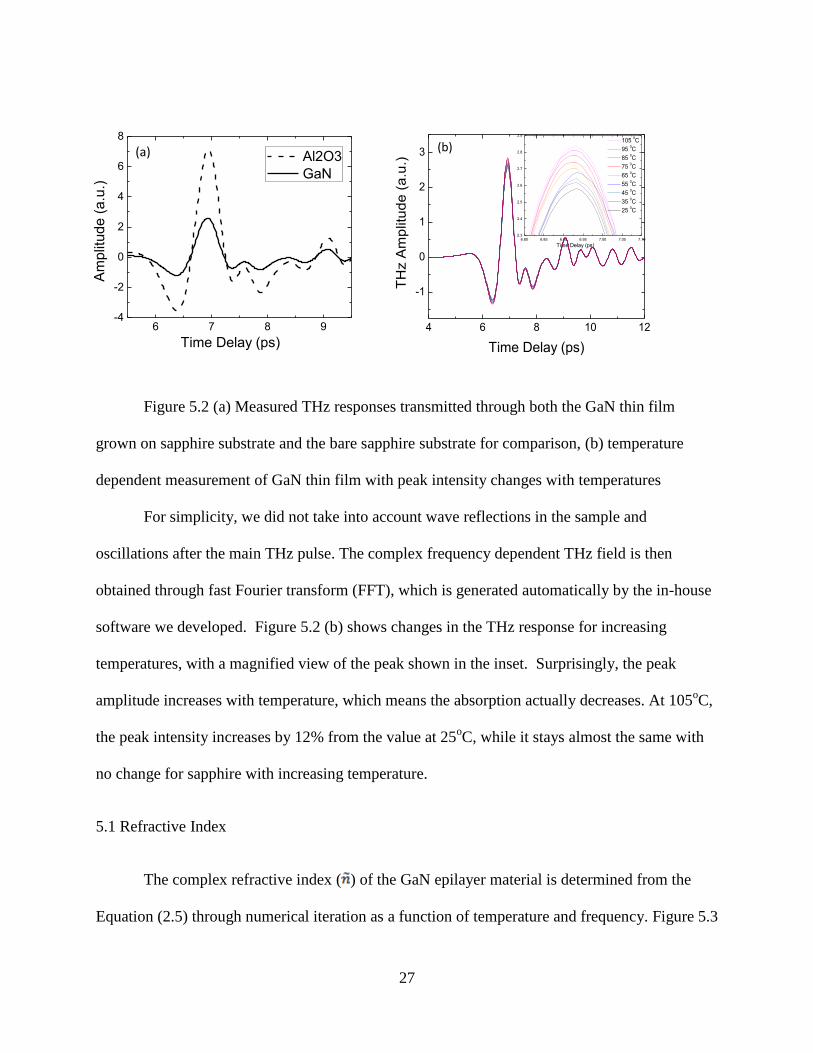
Figure 5.2 (a) Measured THz responses transmitted through both the GaN thin film
grown on sapphire substrate and the bare sapphire substrate for comparison, (b) temperature
dependent measurement of GaN thin film with peak intensity changes with temperatures
For simplicity, we did not take into account wave reflections in the sample and
oscillations after the main THz pulse. The complex frequency dependent THz field is then
obtained through fast Fourier transform (FFT), which is generated automatically by the in-house
software we developed. Figure 5.2 (b) shows changes in the THz response for increasing
temperatures, with a magnified view of the peak shown in the inset. Surprisingly, the peak
amplitude increases with temperature, which means the absorption actually decreases. At 105oC,
the peak intensity increases by 12% from the value at 25oC, while it stays almost the same with
no change for sapphire with increasing temperature.
5.1 Refractive Index
The complex refractive index ( ) of the GaN epilayer material is determined from the
Equation (2.5) through numerical iteration as a function of temperature and frequency. Figure 5.3
6 7 8 9-4
-2
0
2
4
6
8
Am
plit
ud
e (
a.u
.)
Time Delay (ps)
Al2O3
GaN
(a)
6.80 6.85 6.90 6.95 7.00 7.05 7.102.3
2.4
2.5
2.6
2.7
2.8
2.9
Time Delay (ps)
105 0C
95 0C
85 0C
75 0C
65 0C
55 0C
45 0C
35 0C
25 0C
4 6 8 10 12
-1
0
1
2
3
TH
z A
mp
litu
de
(a
.u.)
Time Delay (ps)
(b)
28
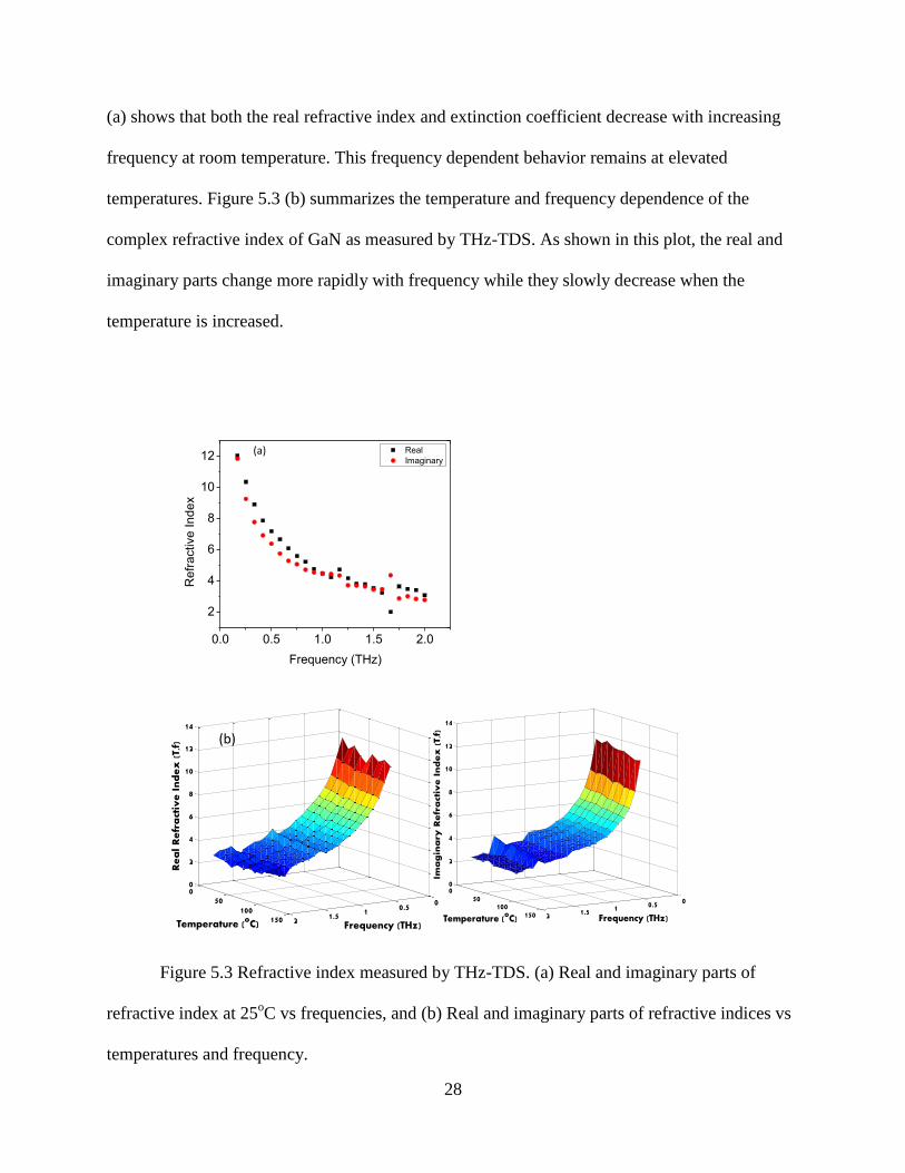
(a) shows that both the real refractive index and extinction coefficient decrease with increasing
frequency at room temperature. This frequency dependent behavior remains at elevated
temperatures. Figure 5.3 (b) summarizes the temperature and frequency dependence of the
complex refractive index of GaN as measured by THz-TDS. As shown in this plot, the real and
imaginary parts change more rapidly with frequency while they slowly decrease when the
temperature is increased.
0.0 0.5 1.0 1.5 2.0
2
4
6
8
10
12 Real
Imaginary
Re
fra
ctive
In
de
x
Frequency (THz)
(a)
00.511.52
050
100150
0
2
4
6
8
10
12
14
Frequency (THz)Temperature (oC)
Re
al
Re
fra
ctiv
e I
nd
ex
(T,
f)
00.511.52
050
100150
0
2
4
6
8
10
12
14
Frequency (THz)Temperature (oC)
Ima
gin
ary
Re
fra
ctiv
e I
nd
ex
(T,
f)(b)
Figure 5.3 Refractive index measured by THz-TDS. (a) Real and imaginary parts of
refractive index at 25oC vs frequencies, and (b) Real and imaginary parts of refractive indices vs
temperatures and frequency.

29
5.2 Conductivity and Fitting
The complex electrical conductivity can be extracted from the measured complex
refractive index by using Equation (3.4) and (3.5), and its real and imaginary parts are plotted in
Figure 5.4 (a) as a function of frequency. Again, both parts vary monotonously with frequency,
but their trends are different. The real conductivity -which is the conventional conductivity-
decreases with frequency. There are a few reports describing a similar behavior. By contrast, the
imaginary conductivity increases with frequency. The complex conductivity was also calculated
as a function of temperature from 25oC to 105
oC. For all temperatures, the frequency
dependency of both real and imaginary parts followed a trend similar to the one shown in Figure
5.4 (a). Figure 5.4 (b) illustrates this for the temperature dependent real conductivity at a few
selected THz frequencies. Interestingly, the real electrical conductivity decreases as temperature
increases: from 25 (-cm)-1
at 25 oC down to 22 (-cm)
-1 at 105 °C (0.5 THz), and from 20.5
(-cm)-1
at 25oC down to 17 (-cm)
-1 at 105 °C (1.5THz).s
0.5 1.0 1.5 2.0-5
0
5
10
15
20
25
30
35
40
Co
nd
uctivity (
cm
)-1
Real
Imaginary
Frequency (THz)
(a)
20 40 60 80 10015
20
25
30
Re
al C
on
du
ctivity (
cm
)-1
Temperature (oC)
0.5 THz
1.0 THz
1.5 THz
2.0 THz
(b)
Figure 5.4 (a) Real and imaginary part of conductivity at 25oC vs frequencies, and (b)
real conductivity vs temperature at selective frequencies.
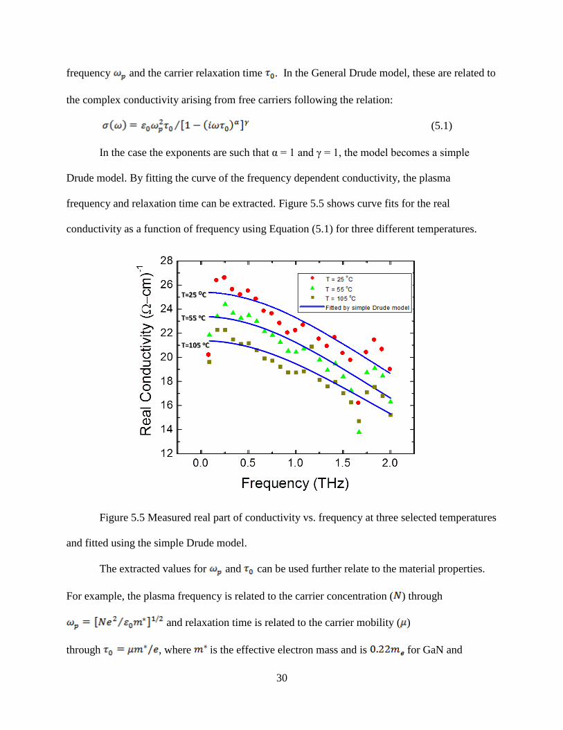
The frequency dependent complex conductivity was fitted using the Drude model [21] to
further analyze carrier dynamics and extract important material parameters, including the plasma
30
frequency and the carrier relaxation time . In the General Drude model, these are related to
the complex conductivity arising from free carriers following the relation:
(5.1)
In the case the exponents are such that α = 1 and γ = 1, the model becomes a simple
Drude model. By fitting the curve of the frequency dependent conductivity, the plasma
frequency and relaxation time can be extracted. Figure 5.5 shows curve fits for the real
conductivity as a function of frequency using Equation (5.1) for three different temperatures.
Figure 5.5 Measured real part of conductivity vs. frequency at three selected temperatures
and fitted using the simple Drude model.
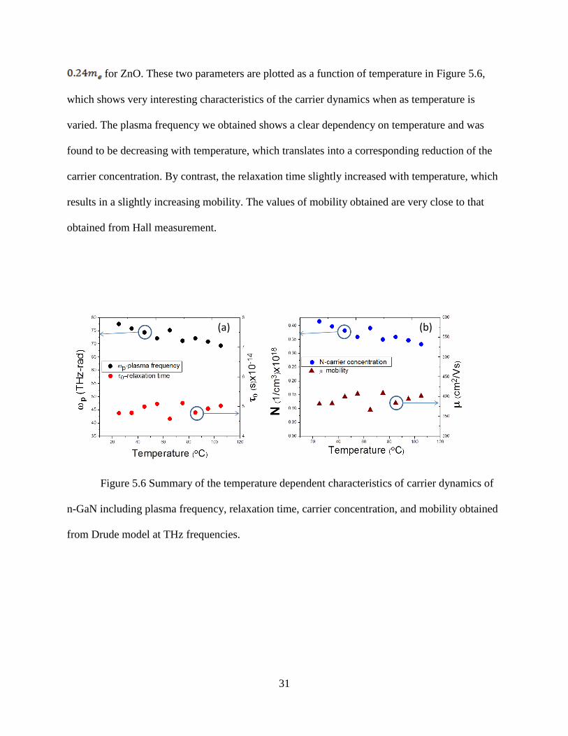
The extracted values for and can be used further relate to the material properties.
For example, the plasma frequency is related to the carrier concentration ( ) through
and relaxation time is related to the carrier mobility ( )
through , where is the effective electron mass and is for GaN and
31
for ZnO. These two parameters are plotted as a function of temperature in Figure 5.6,
which shows very interesting characteristics of the carrier dynamics when as temperature is
varied. The plasma frequency we obtained shows a clear dependency on temperature and was
found to be decreasing with temperature, which translates into a corresponding reduction of the
carrier concentration. By contrast, the relaxation time slightly increased with temperature, which
results in a slightly increasing mobility. The values of mobility obtained are very close to that
obtained from Hall measurement.
(a) (b)
Figure 5.6 Summary of the temperature dependent characteristics of carrier dynamics of
n-GaN including plasma frequency, relaxation time, carrier concentration, and mobility obtained
from Drude model at THz frequencies.
32
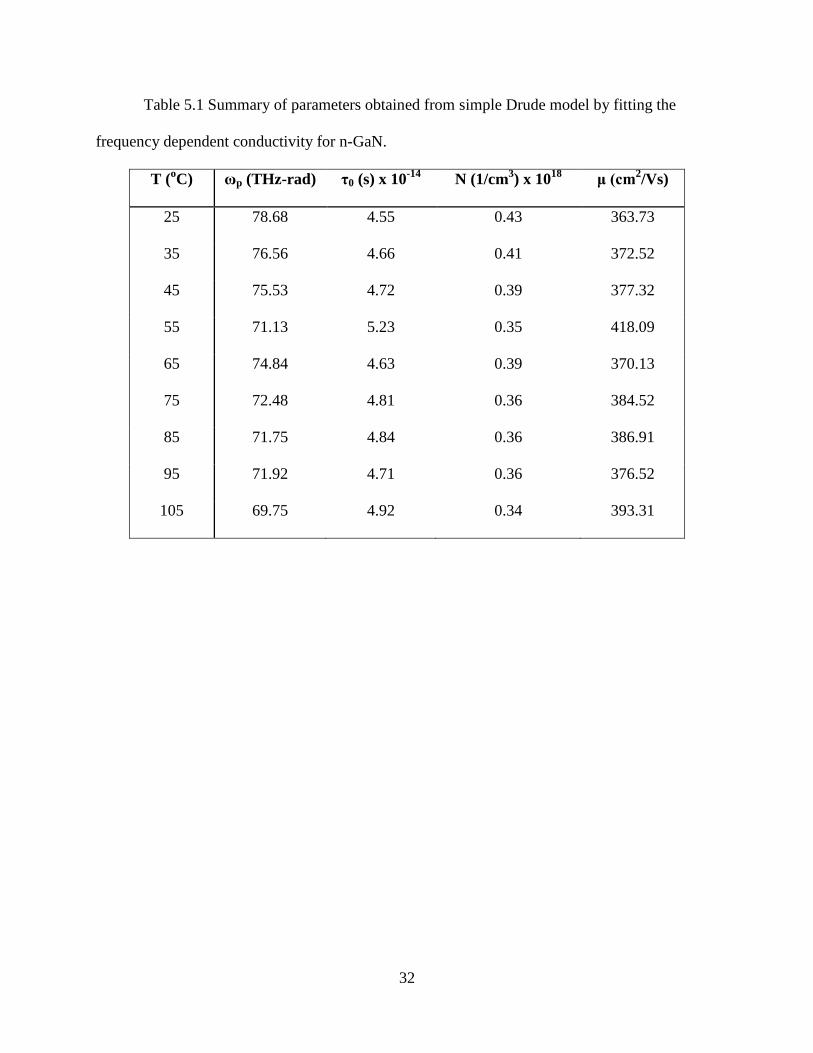
Table 5.1 Summary of parameters obtained from simple Drude model by fitting the
frequency dependent conductivity for n-GaN.
T (oC) ωp (THz-rad) τ0 (s) x 10
-14 N (1/cm
3) x 10
18 μ (cm
2/Vs)
25 78.68 4.55 0.43 363.73
35 76.56 4.66 0.41 372.52
45 75.53 4.72 0.39 377.32
55 71.13 5.23 0.35 418.09
65 74.84 4.63 0.39 370.13
75 72.48 4.81 0.36 384.52
85 71.75 4.84 0.36 386.91
95 71.92 4.71 0.36 376.52
105 69.75 4.92 0.34 393.31
33
CHAPTER 6
ZnO NANOWIRES
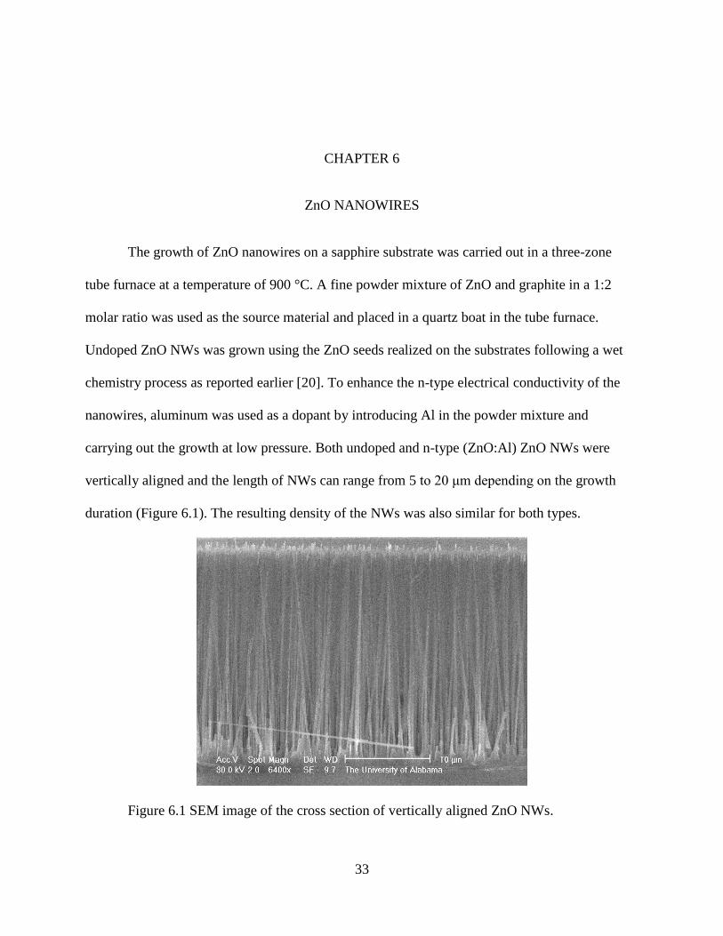
The growth of ZnO nanowires on a sapphire substrate was carried out in a three-zone
tube furnace at a temperature of 900 °C. A fine powder mixture of ZnO and graphite in a 1:2
molar ratio was used as the source material and placed in a quartz boat in the tube furnace.
Undoped ZnO NWs was grown using the ZnO seeds realized on the substrates following a wet
chemistry process as reported earlier [20]. To enhance the n-type electrical conductivity of the
nanowires, aluminum was used as a dopant by introducing Al in the powder mixture and
carrying out the growth at low pressure. Both undoped and n-type (ZnO:Al) ZnO NWs were
vertically aligned and the length of NWs can range from 5 to 20 μm depending on the growth
duration (Figure 6.1). The resulting density of the NWs was also similar for both types.
Figure 6.1 SEM image of the cross section of vertically aligned ZnO NWs.
34
6.1 Undoped ZnO NWs
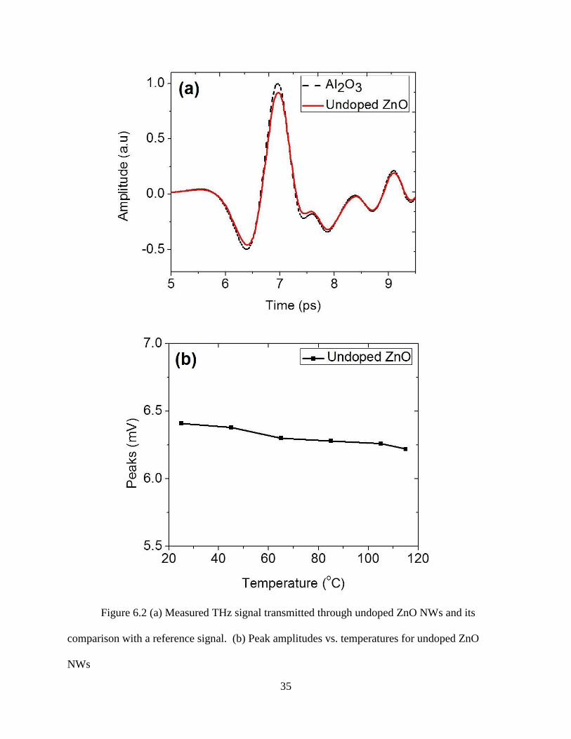
The transmitted THz electric field through the ZnO NWs did not change too much for
undoped ZnO NW as shown in Figure 6.2(a). The peak amplitude was about 90 % that of the
THz wave transmitted through the bare sapphire substrate (“reference”). Figure 6.2(b) shows the
THz transmitted wave peak amplitudes as a function of temperature for undoped NWs. It
decreases as the temperature increases. It is noted that this behavior is different from what was
observed in n-GaN in the previous section. However, the amount of decrease is small at the same
time.
35
Figure 6.2 (a) Measured THz signal transmitted through undoped ZnO NWs and its
comparison with a reference signal. (b) Peak amplitudes vs. temperatures for undoped ZnO
NWs

36
6.1.1 Refractive Index
Since the wavelength of the light used in this study is much larger than the diameter of
ZnO NWs, the refractive index of ZnO NW cannot simply be subtracted out from the refractive
index of the ZnO NW/air composite. Therefore, effective medium theory should be taken into
account [22]. This theory is mostly used to calculate the permittivity of a composite material
while the permittivity and volume fraction of each of the individual components. One of the most
commonly used effective medium theories is the Bruggeman effective medium approximation
(EMA) [23] given by
(6.1)
where, is the volume fraction of NWs from the density of NWs, is the permittivity of the
composite (ZnO NW/air), is the matrix permittivity which is 1 (air) in this study, is the
particle permittivity (ZnO NWs), and K is a geometric factor which is 1 for an array of cylinders
with its axis collinear with the incident radiation and 2 for spherical nanoparticles. The
Bruggeman EMA can be used in reverse to calculate the permittivity of one component (ZnO
NWs) while those of both the other component (air) and the composite (ZnO NW/air) are known.
Rearranging Equation (6.1) to solve , with =1 and K =1, one gets:
(6.2)
First, the refractive index of the composite (ZnO NW/air) was determined with the same
numerical method described in GaN section (Equation (2.5)). Then, by using the relation
between the complex refractive index and permittivity (Equation (3.4) and (3.5)), the complex
37
refractive index of ZnO NW was extracted from the composite (ZnO NW/air). The same process
was applied in the case of all temperatures in order to yield a temperature dependent refractive
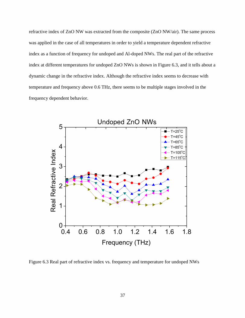
index as a function of frequency for undoped and Al-doped NWs. The real part of the refractive
index at different temperatures for undoped ZnO NWs is shown in Figure 6.3, and it tells about a
dynamic change in the refractive index. Although the refractive index seems to decrease with
temperature and frequency above 0.6 THz, there seems to be multiple stages involved in the
frequency dependent behavior.
0.4 0.6 0.8 1.0 1.2 1.4 1.6 1.80
1
2
3
4
5
Re
al R
efr
active
In
de
x
Frequency (THz)
T=25oC
T=45oC
T=65oC
T=85oC
T=105oC
T=115oC
Undoped ZnO NWs
Figure 6.3 Real part of refractive index vs. frequency and temperature for undoped NWs
38
6.1.2 Conductivity and Fitting
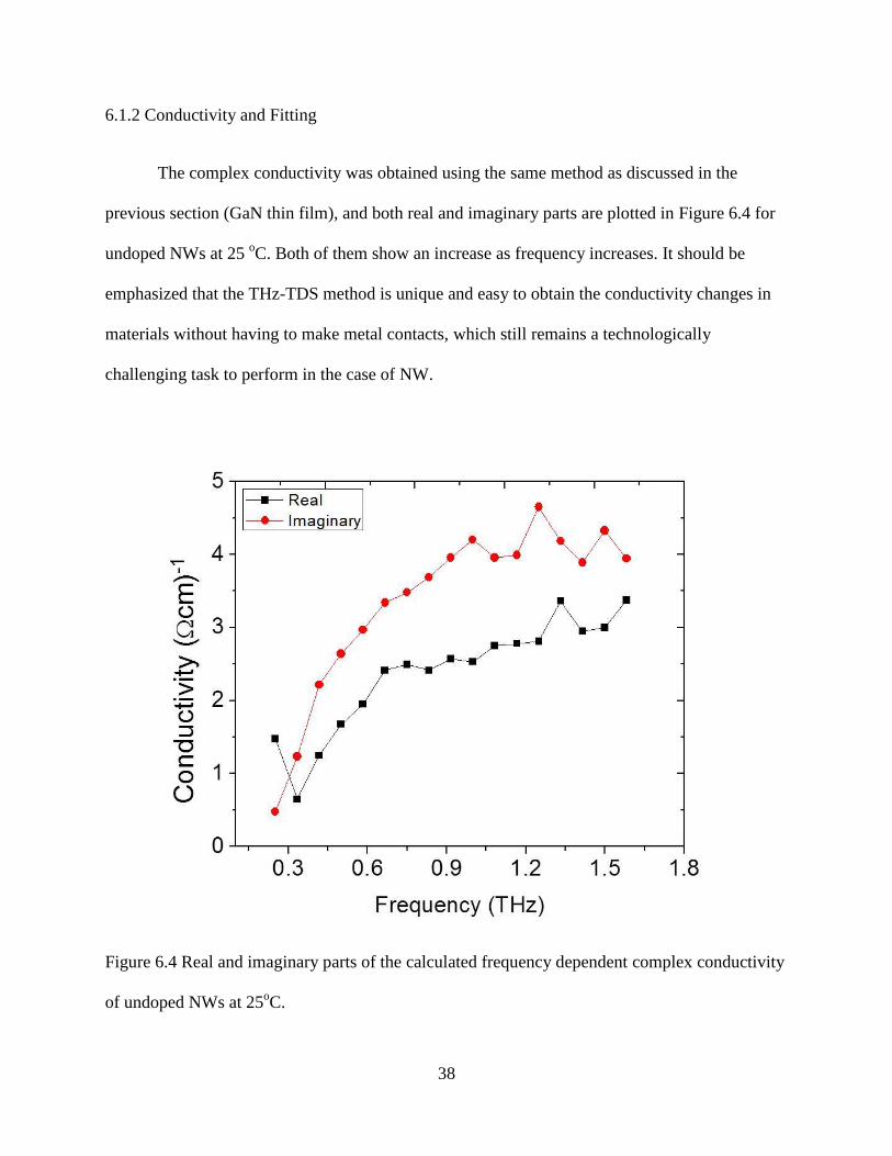
The complex conductivity was obtained using the same method as discussed in the
previous section (GaN thin film), and both real and imaginary parts are plotted in Figure 6.4 for
undoped NWs at 25 oC. Both of them show an increase as frequency increases. It should be
emphasized that the THz-TDS method is unique and easy to obtain the conductivity changes in
materials without having to make metal contacts, which still remains a technologically
challenging task to perform in the case of NW.
Figure 6.4 Real and imaginary parts of the calculated frequency dependent complex conductivity
of undoped NWs at 25oC.

39
The conductivity as a function of frequency for undoped NWs was calculated at selected
temperatures and shown in Figure 6.5. At 25 oC, the conductivity is increasing with the
frequency. But at the elevated temperature, a multiple stage process seems to appear in the
frequency dependent conductivity, similar to the frequency dependence of the refractive index.
Figure 6.5 Real conductivity and curve fit (at 25oC) using the Drude-Smith model for undoped
NWs at different temperatures.
To fit the calculated conductivity in ZnO NWS, we had to use the Drude-Smith model,
which is described by the following expression,
40
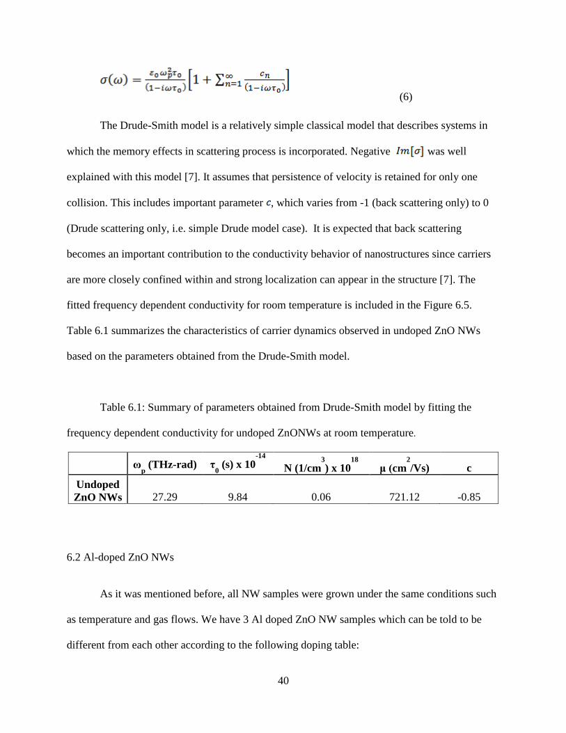
The Drude-Smith model is a relatively simple classical model that describes systems in
which the memory effects in scattering process is incorporated. Negative was well
explained with this model [7]. It assumes that persistence of velocity is retained for only one
collision. This includes important parameter , which varies from -1 (back scattering only) to 0
(Drude scattering only, i.e. simple Drude model case). It is expected that back scattering
becomes an important contribution to the conductivity behavior of nanostructures since carriers
are more closely confined within and strong localization can appear in the structure [7]. The
fitted frequency dependent conductivity for room temperature is included in the Figure 6.5.
Table 6.1 summarizes the characteristics of carrier dynamics observed in undoped ZnO NWs
based on the parameters obtained from the Drude-Smith model.
Table 6.1: Summary of parameters obtained from Drude-Smith model by fitting the
frequency dependent conductivity for undoped ZnONWs at room temperature.
ωp (THz-rad) τ
0 (s) x 10
-14
N (1/cm3
) x 1018
μ (cm2
/Vs) c
Undoped
ZnO NWs 27.29 9.84 0.06 721.12 -0.85
6.2 Al-doped ZnO NWs
As it was mentioned before, all NW samples were grown under the same conditions such
as temperature and gas flows. We have 3 Al doped ZnO NW samples which can be told to be
different from each other according to the following doping table:
(6)
41
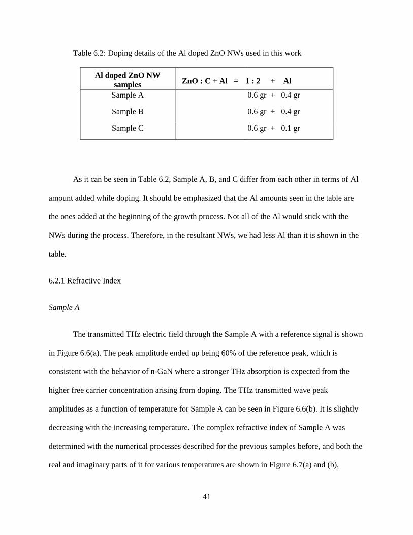
Table 6.2: Doping details of the Al doped ZnO NWs used in this work
Al doped ZnO NW
samples ZnO : C + Al = 1 : 2 + Al
Sample A
0.6 gr + 0.4 gr
Sample B
0.6 gr + 0.4 gr
Sample C
0.6 gr + 0.1 gr
As it can be seen in Table 6.2, Sample A, B, and C differ from each other in terms of Al
amount added while doping. It should be emphasized that the Al amounts seen in the table are
the ones added at the beginning of the growth process. Not all of the Al would stick with the
NWs during the process. Therefore, in the resultant NWs, we had less Al than it is shown in the
table.
6.2.1 Refractive Index
Sample A
The transmitted THz electric field through the Sample A with a reference signal is shown
in Figure 6.6(a). The peak amplitude ended up being 60% of the reference peak, which is
consistent with the behavior of n-GaN where a stronger THz absorption is expected from the
higher free carrier concentration arising from doping. The THz transmitted wave peak
amplitudes as a function of temperature for Sample A can be seen in Figure 6.6(b). It is slightly
decreasing with the increasing temperature. The complex refractive index of Sample A was
determined with the numerical processes described for the previous samples before, and both the
real and imaginary parts of it for various temperatures are shown in Figure 6.7(a) and (b),
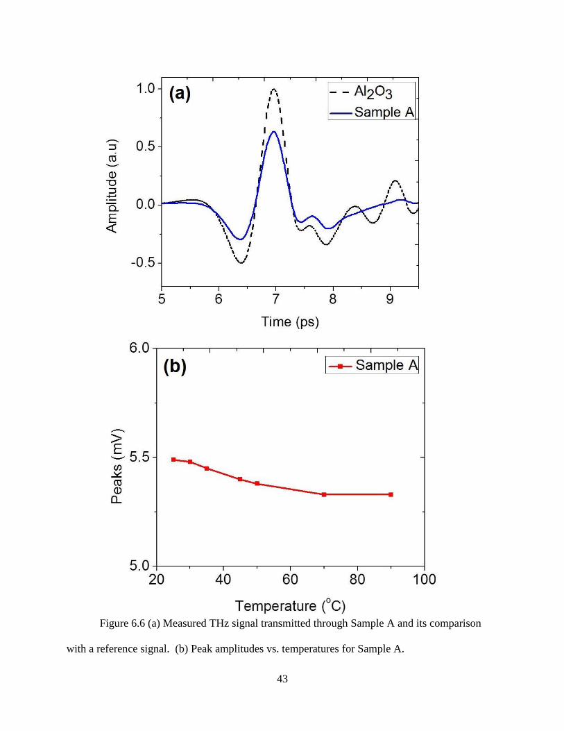
42
respectively. Figure 6.7(a) shows that the real part of the complex refractive index smoothly
decreases both as the frequency increases and as the temperature increases. At higher
temperature, the decrease with frequency becomes more pronounced. In addition, the
temperature dependency shows a distinct feature. Indeed, there were only minimal changes in
the refractive index with temperature at lower frequencies (below 0.6 THz), while the changes
were more discernible as both temperature and frequency increase (above 0.6 THz). As it is seen
in Figure 6.7(b), the imaginary part of the complex refractive index clearly decreases with the
increasing frequency; however, we cannot talk about a temperature dependent behavior for the
imaginary part. It remains almost same for all temperatures.
43
Figure 6.6 (a) Measured THz signal transmitted through Sample A and its comparison
with a reference signal. (b) Peak amplitudes vs. temperatures for Sample A.

44
Figure 6.7 (a) Real and (b) Imaginary part of refractive index vs. frequency and
temperature for Sample A.
45
Sample B
Figure 6.8(a) shows the time domain THz electric field transmitted through the Sample B
with a reference signal. The peak amplitude is almost the same with the peak of the reference
signal which is similar to the case seen for undoped ZnO NWs. Even though Sample B had the
same amount of Al with Sample A at the beginning of the growth process as seen in Table 6.2,
the behavior in Figure 6.8(a) is similar to the behavior of undoped ZnO NWs as seen in Figure
6.2(a). That leads us to infer that most of the Al was lost during the growth process and only
little amount was stuck to the nanowires. The peak amplitudes of the transmitted THz waves at
selected temperatures are plotted versus temperature in Figure 6.8(b). There is a slight decrease
in peaks while the temperature increases.
The real and imaginary parts of the determined complex refractive index of Sample B are
plotted for selected temperatures in Figure 6.9(a) and (b), respectively. It can be clearly seen in
Figure 6.9(a) that the real part of the refractive index decreases with the increasing temperature
while it can be assumed to be independent of the frequency except tiny oscillations. The
imaginary component of the refractive index decreases with the increasing frequency while it
increases with the temperature, shown in Figure 6.9(b). In the frequency region lower than 1.0
THz, both frequency and temperature dependencies of the imaginary component are stronger. As
the frequency increases (above 1.0 THz), the decrement versus frequency gets smaller, and the
temperature dependency becomes less distinct.

46
Figure 6.8 (a) Measured THz signal transmitted through Sample B and its comparison
with a reference signal. (b) Peak amplitudes vs. temperatures for Sample B.

47
Figure 6.9 (a) Real and (b) Imaginary part of refractive index vs. frequency and
temperature for Sample B.
48
Sample C
The time domain THz wave transmitted through the Sample C and the reference signal
are shown in Figure 6.10(a). In this case, the peak amplitude is again about %90 of the reference
signal just like it was observed in undoped ZnO NW and Sample B. That let us make a result
such that Sample B and C are less doped than Sample A. The temperature dependency of the
peak amplitudes of the THz waves is plotted in Figure 6.10(b). The peak amplitude decreases
with the increasing temperature.
Figure 6.11(a) and (b) are the real and imaginary components of the complex refractive
index of Sample C determined through numerical iteration process. Figure 6.11(a) shows that the
real component of the complex refractive index decreases both with increasing frequency and
temperature. Below 0.6 THz, frequency dependency is much stronger than the temperature
dependency while they are almost equal above 0.6 THz. The imaginary part of the refractive
index shown in Figure 6.11(b) has almost the same behavior as the real part in terms of
frequency dependency. However, the temperature dependent behavior of the imaginary part is
the opposite of the behavior of the real part: it increases with the increasing temperature, instead.
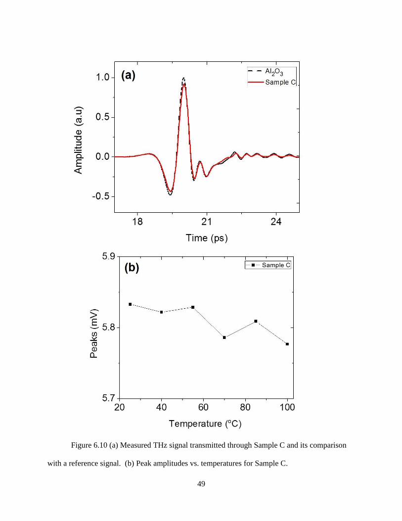
49
Figure 6.10 (a) Measured THz signal transmitted through Sample C and its comparison
with a reference signal. (b) Peak amplitudes vs. temperatures for Sample C.

50
Figure 6.11 (a) Real and (b) Imaginary part of refractive index vs. frequency and
temperature for Sample C.

51
6.2.2 Conductivity and Fitting
Sample A
The real and imaginary parts of the calculated complex conductivity are plotted in Figure
6.12 for Sample A at room temperature. Both parts show similar trend with the increasing
frequency. They increase versus frequency almost with the same slope, but with different
amplitudes. Comparing the real conductivities of undoped ZnO NW (Figure 6.4) and Al doped
ZnO NW (Sample A, Figure 6.12), it is clearly visible that the electrical conductivity increases
by a factor of ~3 at THz frequencies due to the incorporation of Al into the ZnO NWs.
Figure 6.12 Real and imaginary parts of the calculated frequency dependent complex
conductivity of Sample A at 25oC.
52
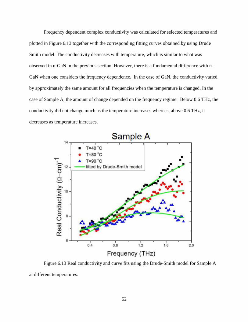
Frequency dependent complex conductivity was calculated for selected temperatures and
plotted in Figure 6.13 together with the corresponding fitting curves obtained by using Drude
Smith model. The conductivity decreases with temperature, which is similar to what was
observed in n-GaN in the previous section. However, there is a fundamental difference with n-
GaN when one considers the frequency dependence. In the case of GaN, the conductivity varied
by approximately the same amount for all frequencies when the temperature is changed. In the
case of Sample A, the amount of change depended on the frequency regime. Below 0.6 THz, the
conductivity did not change much as the temperature increases whereas, above 0.6 THz, it
decreases as temperature increases.
Figure 6.13 Real conductivity and curve fits using the Drude-Smith model for Sample A
at different temperatures.

53
Sample B
Figure 6.14 shows both real and imaginary components of the calculated frequency
dependent complex conductivity at room temperature. Imaginary part can be assumed to be not
changing with the increasing frequency except tiny oscillations. The real part seems to have two
distinct regions: below 1.0 THz and above 1.0 THz. It can be considered to be frequency
independent in each region (below and above 1.0 THz) with a higher value in the second region
(above 1.0 THz). Again, the conductivity’s being as low as the one of the undoped ZnO NW
supports the previous outcome from Figure 6.8(a) that Sample B has very little amount of Al
(almost undoped).
Figure 6.14 Real and imaginary parts of the calculated frequency dependent complex
conductivity of Sample B at 25oC.
54
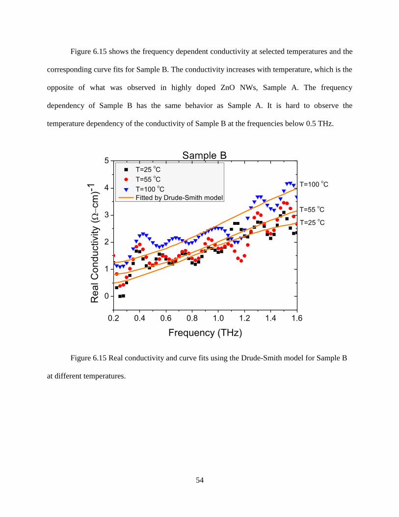
Figure 6.15 shows the frequency dependent conductivity at selected temperatures and the
corresponding curve fits for Sample B. The conductivity increases with temperature, which is the
opposite of what was observed in highly doped ZnO NWs, Sample A. The frequency
dependency of Sample B has the same behavior as Sample A. It is hard to observe the
temperature dependency of the conductivity of Sample B at the frequencies below 0.5 THz.
0.2 0.4 0.6 0.8 1.0 1.2 1.4 1.6
0
1
2
3
4
5
T=100 oC
T=55 oC
Re
al C
on
du
ctivity (cm
)-1
Frequency (THz)
T=25 oC
T=55 oC
T=100 oC
Fitted by Drude-Smith model
T=25 oC
Sample B
Figure 6.15 Real conductivity and curve fits using the Drude-Smith model for Sample B
at different temperatures.
55
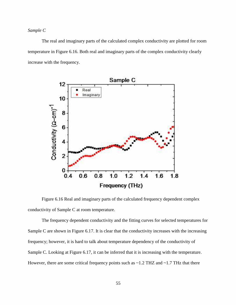
Sample C
The real and imaginary parts of the calculated complex conductivity are plotted for room
temperature in Figure 6.16. Both real and imaginary parts of the complex conductivity clearly
increase with the frequency.
Figure 6.16 Real and imaginary parts of the calculated frequency dependent complex
conductivity of Sample C at room temperature.
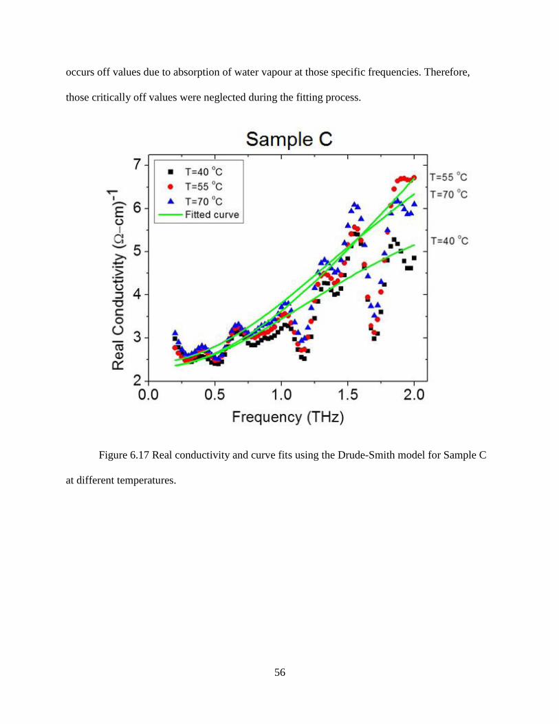
The frequency dependent conductivity and the fitting curves for selected temperatures for
Sample C are shown in Figure 6.17. It is clear that the conductivity increases with the increasing
frequency; however, it is hard to talk about temperature dependency of the conductivity of
Sample C. Looking at Figure 6.17, it can be inferred that it is increasing with the temperature.
However, there are some critical frequency points such as ~1.2 THZ and ~1.7 THz that there
56
occurs off values due to absorption of water vapour at those specific frequencies. Therefore,
those critically off values were neglected during the fitting process.
Figure 6.17 Real conductivity and curve fits using the Drude-Smith model for Sample C
at different temperatures.
57
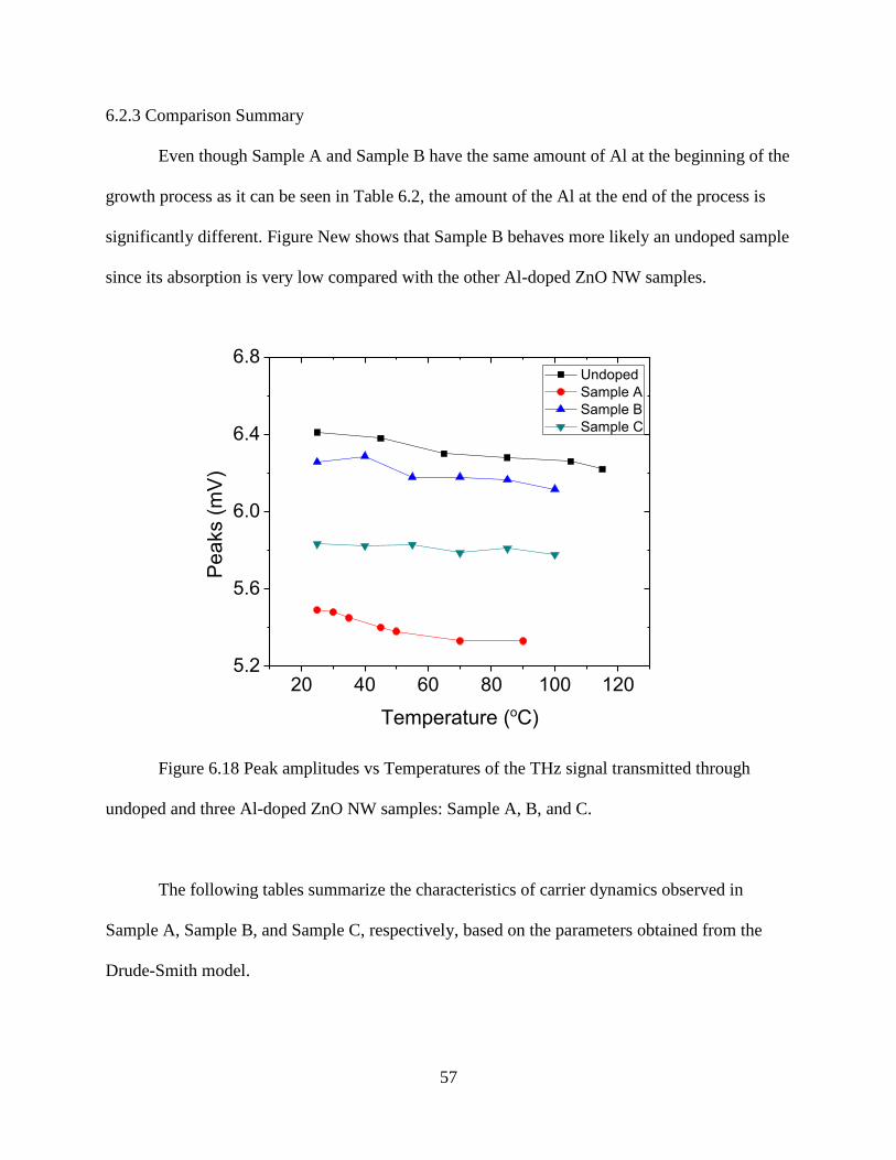
6.2.3 Comparison Summary
Even though Sample A and Sample B have the same amount of Al at the beginning of the
growth process as it can be seen in Table 6.2, the amount of the Al at the end of the process is
significantly different. Figure New shows that Sample B behaves more likely an undoped sample
since its absorption is very low compared with the other Al-doped ZnO NW samples.
20 40 60 80 100 1205.2
5.6
6.0
6.4
6.8
Pe
aks (
mV
)
Temperature (oC)
Undoped
Sample A
Sample B
Sample C
Figure 6.18 Peak amplitudes vs Temperatures of the THz signal transmitted through
undoped and three Al-doped ZnO NW samples: Sample A, B, and C.
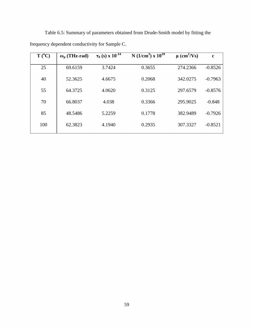
The following tables summarize the characteristics of carrier dynamics observed in
Sample A, Sample B, and Sample C, respectively, based on the parameters obtained from the
Drude-Smith model.

58
Table 6.3: Summary of parameters obtained from Drude-Smith model by fitting the
frequency dependent conductivity for Sample A.
T (o
C) ωp (THz-rad) τ
0 (s) x 10
-14
N (1/cm3
) x 1018
μ (cm2
/Vs) c
25 54.42 7.29 0.22 534.43 -0.67
40 74.18 5.17 0.42 379.01 -0.74
55 60.00 5.29 0.27 387.44 -0.60
70 63.29 5.97 0.30 437.58 -0.67
80 57.29 6.68 0.25 489.27 -0.68
90 50.85 7.45 0.20 545.76 -0.61
Table 6.4: Summary of parameters obtained from Drude-Smith model by fitting the
frequency dependent conductivity for Sample B.
T (oC) ωp (THz-rad) τ0 (s) x 10
-14 N (1/cm
3) x 10
18 μ (cm
2/Vs) c
25 29.55 7.40 0.07 542.56 -0.93
40 41.15 5.34 0.13 391.51 -0.91
55 42.20 5.26 0.13 385.58 -0.91
70 42.46 5.79 0.14 423.99 -0.93
85 48.94 4.32 0.18 316.67 -0.91
100 46.98 5.23 0.17 383.29 -0.89
59
Table 6.5: Summary of parameters obtained from Drude-Smith model by fitting the
frequency dependent conductivity for Sample C.
T (oC) ωp (THz-rad) τ0 (s) x 10
-14 N (1/cm
3) x 10
18 μ (cm
2/Vs) c
25 69.6159 3.7424 0.3655 274.2366 -0.8526
40 52.3625 4.6675 0.2068 342.0275 -0.7963
55 64.3725 4.0620 0.3125 297.6579 -0.8576
70 66.8037 4.038 0.3366 295.9025 -0.848
85 48.5486 5.2259 0.1778 382.9489 -0.7926
100 62.3823 4.1940 0.2935 307.3327 -0.8521

60
CHAPTER 7
CONCLUSION
We have presented a comprehensive study of the temperature dependent carrier dynamics
of n-GaN and ZnO NWs based on THz-Time Domain Spectroscopy measurements.
Spectroscopy measurements were performed for each sample at elevated temperatures by using a
heating stage added to sample mount and a feedback loop to verify the sample temperature. To
analyze the measured signals, computational methods were developed. Combining experimental
measurements and numerical calculations, the complex refractive index, dielectric function, and
conductivity of n-GaN, undoped ZnO NWs, and three Al-doped ZnO NW samples with different
doping ratios were obtained. The unique temperature dependent behaviors of these material
parameters were studied at THz frequencies. We were able to observe how different doping
ratios would affect the material parameters. Different fitting processes were developed for GaN
thin film and ZnO NWs separately due to their significantly different conductivity behavior.
Further analysis of temperature dependent carrier dynamics were obtained considering both the
Drude and the Drude-Smith models in order to extract the plasma frequency, relaxation time,
carrier concentration and mobility.
61
REFERENCES
[1] K. P. Cheung and D. H. Auston, Infrared Phys. 26, 23 (1986).
[2] D. Grischkowsky, S. Keiding, M. van Exter, and Ch. Fattinger, J. Opt. Soc. Am. B 7, 2006
(1990).
[3] B. Ferguson and X.-C. Zhang, Nature Mater. 1, 26 (2002).
[4] M. Tonouchi, Nat. Photonics 1, 97 (2007).
[5] M. Van Exter, and D. Grischkowsky, Phys. Rev. B, 41, 1990, pp. 12140-12149.
[6] Charles A. Schmuttenmaer, Chem. Rev. 104, 1759-1779 (2004).
[7] Baxter, J.B.; Schmuttenmaer, C.A., J Phys Chem B 2006, 110, 25229.
[8] Tsong-Ru Tsai, Shi-Jie Chen, Chih-Fu Chang, Sheng-Hsien Hsu, Tai-Yuan Lin, and Cheng-
Chung Chi, Opt. Express 14, 4898-4907 (2006)
[9] Jiaguang Han, Abul K. Azad , and Weili Zhang, Journal of Nanoelectronics and
Optoelectronics, Vol. 2, 222-233 (2007)
[10] S. Nakamura, T. Mukai, and M. Senoh, Appl. Phys. Lett. 64, 1687-1689 (1994).
[11] K. S. Ramaiah, Y. K. Su, S. J. Chang, B. Kerr, H. P. Liu, and I. G. Chen, Appl. Phys. Lett.
84, 3307-3309 (2004).
[12] S. Nakamura, M. Senoh, S. Nagahama, N. Iwasa, T. Yamada, T. Matsushita, H. Kiyoku,
and Y. Sugimoto, Jpn. J. Appl. Phys., Part 2, 35, L74-L76 (1996).
[13] F. A. Ponce, and D. P. Bour, Nature 386, 351-359, (1997).
[14] Ü. Özgür, Ya. I. Alivov, C. Liu, A. Teke, M. A. Reshchikov, S. Doğan, V. Avrutin, S.-J.
Cho, and H. Morkoç, J. Appl. Phys. 98, 041301 (2005).
[15] R. Gaska, J. W. Yang, A. Osinsky, Q. Chen, M. A. Khan, A. O. Orlov, G. L. Snider, and M.
S. Shur, Appl. Phys. Lett. 72, 707-709 (1998).
[16] S. J. Pearton, J. C. Zolper, R. J. Shul, and F. Ren, “GaN: Processing, defects, and devices,”
J. Appl. Phys. 86, 1-78 (1999).
[17] H. Morkoc, S. Strite, G. B. Gao, M. E. Lin, B. Sverdlov, and M. Burns, J. Appl. Phys. 76,
1363-1398 (1994).

62
[18] Wan, Q.; Li, Q. H.; Chen, Y. J.; Wang, T. H.; He, X. L.; Li, J. P.; Lin, C. L., Appl. Phys.
Lett. 84 (2004) 3654.
[19] B Liu, D.H Lim, M Lachab, A Jia, K Takahashi and A Yoshikawa, IPAP Conf. Ser. 1
(2000), 133.
[20] R. N. Gayen, R. Bhar, A. K. Pal, Indian Journal of Pure & Applied Physics 48, June 2010,
pp. 385-393
[21] N. V. Smith, Phys. Rev. B 64, 155106 (2001).
[22] Choy, T. C. Effective Medium Theory: Principles and Applications; Clarendon Press:
Oxford, U. K., 1999.
[23] Bruggeman, D. A. G., Ann. Phys. 24 (1935) 636.
[24] L. Duvillaret, F. Garet, J.L. Coutaz, IEEE Journal of Selected Topics in Quantum
Electronics, 2 (1996), pp. 739–746