characterization of human-induced vibrations
TRANSCRIPT
University of South CarolinaScholar Commons
Theses and Dissertations
2016
Characterization of Human-Induced VibrationsBenjamin Thomas DavisUniversity of South Carolina
Follow this and additional works at: https://scholarcommons.sc.edu/etd
Part of the Civil Engineering Commons
This Open Access Dissertation is brought to you by Scholar Commons. It has been accepted for inclusion in Theses and Dissertations by an authorizedadministrator of Scholar Commons. For more information, please contact [email protected].
Recommended CitationDavis, B. T.(2016). Characterization of Human-Induced Vibrations. (Doctoral dissertation). Retrieved fromhttps://scholarcommons.sc.edu/etd/3770

Characterization of Human-Induced Vibrations
by
Benjamin Thomas Davis
Bachelor of ScienceUniversity of South Carolina 2013
Master of ScienceUniversity of California, Berkeley 2014
Submitted in Partial Fulfillment of the Requirements
for the Degree of Doctor of Philosophy in
Civil Engineering
College of Engineering and Computing
University of South Carolina
2016
Accepted by:
Juan Caicedo, Major Professor
Victor Hirth, Committee Member
Robert Mullen, Committee Member
Dimitris Rizos, Committee Member
Lacy Ford, Senior Vice Provost and Dean of Graduate Studies

c© Copyright by Benjamin Thomas Davis, 2016All Rights Reserved.
ii

Dedication
To all those who take the road less traveled by,
it makes all the difference [1].
iii

Acknowledgments
Funding
This work is partially supported by a grant from the University of South Carolina
Magellan Scholar Program, and additional partial support is provided by a grant
from the Alzheimer’s Association (ETAC-10-174499).
This work was supported in part by VISN 7 from the United States (US) Depart-
ment of Veterans Affairs Health Services Research and Development Service. The
contents do not represent the views of the US Department of Veterans Affairs or the
US Government.
This material is based upon work supported by the National Science Foundation
Graduate Research Fellowship Program under Grant Number 1450810. Any opinions,
findings, and conclusions or recommendations expressed in this material are those
of the author(s) and do not necessarily reflect the views of the National Science
Foundation.
Appreciation
My thanks to the following who are presented in no particular order and with the
role I knew them in:
• Dr. Juan Caicedo (USC Professor) for his invaluable guidance, support, andencouragement since the beginning of my college career;
• Dr. Victor Hirth (PH Medical Director) for his collaboration and guidance onthe project;
• Dr. Bruce Easterling (VAMC Doctor) for his collaboration on the hospitalstudy;
iv

• Dr. Charles Pierce (USC Professor) for inspiring me to be a civil engineerduring the Carolina Master Scholars program;
• Johannio Marulanda, Glen Weiger, Gustavo Ospina, and Grady Mathews(PhD Candidates) for helping me thoroughly understand various aspects ofengineering;
• Ramin Madarshahian, Albert Ortiz, and Yohanna Mejia (PhD Candidates)for helping refine ideas and conquer stubborn math problems;
• Diego Arocha (MS Student) for creating a benchmark dataset comprising 3575human-induced vibrations records;
• Michael Fernandez (BS Student) for building the steel test frame FEEL wasinitially tested on;
• Andrew MacMillan (BS Student) for his help testing the monitoring systembefore deployment;
• Robert Boykin (BS Student) for lending his computer science skills to helpdevelop the monitoring system;
• Minji Moon (High School Student) for her aid in the initial experiments todevelop FEEL;
• Davis Borucki (High School Student) for his aid in the initial experiments todevelop FEEL;
• Laney Patterson (High School Student) for being a joy summer after summerhelping with experiments;
• Emily Cranwell (Writing Center MS Student) for her Englishgrammar/spelling/writing review and tips so my proposal and dissertationwould sound even better;
• Mackenzie Roman (Nuclear Engineer) for her upbeat encouragement and fooddeliveries;
• Eric and Diane Davis (My Parents) for encouraging me to reach for the stars;
• Emily Davis (My Sister) for her encouragement and support, and keeping megrounded;
• the many study participants across the state of South Carolina;
• countless teachers;
• and all those who kept me going through your encouragement and support.
v

Abstract
In the US alone, 20% of citizens will be over the age of 65 by the year 2030, and the
largest challenge facing this growing demographic is not a new disease but a simple
motion - the fall. These events are the premier cause of fatal and nonfatal injuries. In
fact, a fall is so common that every 17 seconds an older adult is treated for fall-related
injuries, and every 30 minutes, an older adult dies from fall complications. Research
has shown a positive outcome of a fall event is largely dependent on the immediate
response (<30 minutes) and rescue of the person.
This work explores the concept of utilizing structural vibrations to detect human
falls for rapid rescue response. A human-induced vibration monitoring system is de-
veloped on the principles of the ideal fall detection system. The system was installed
throughout the William Jennings Bryan Dorn Veteran’s Administration Medical Cen-
ter (VAMC) and a private four person family’s residence to collect real world human-
induced vibrations. Installation resulted in the recording of 16 human falls and 45,000
acceleration events, expanding the database to 220,597 events as of 2016 February
1. This and other information are recorded according to the data management plan
presented within to enable future study of human activity from vibrations.
For a successful fall detection system implementation, the accelerometers need
the ability to discern good signals to reduce the amount of data analyzed. A method
of signal categorization using Support Vector Machines is explored to this end, with
96.8% accuracy over 100 trials. Following signal selection, the ability to detect a fall
regardless of the distance from the event to the accelerometer becomes paramount,
and is overcome with the introduction of the Force Estimation and Event Localization
vi

(FEEL) Algorithm. The algorithm allows structures to ‘FEEL’ an impact, such as
a fall, boasting 96.4% accuracy in locating the impact in over 3575 impacts of eight
different types, and a 99% confidence interval for being within -2.0% ± 1.3% of
the actual force magnitude. The strength of the algorithm is that it intrinsically
embeds the properties of any structure and does not require time synchronization
of sensors. Since FEEL operates in the frequency domain, an Environments For
Fostering Effective Critical Thinking (EFFECT) active learning module is included
to aid in educating future learners.
vii

Table of Contents
Dedication . . . . . . . . . . . . . . . . . . . . . . . . . . . . . . . . . . iii
Acknowledgments . . . . . . . . . . . . . . . . . . . . . . . . . . . . . iv
Abstract . . . . . . . . . . . . . . . . . . . . . . . . . . . . . . . . . . . vi
List of Tables . . . . . . . . . . . . . . . . . . . . . . . . . . . . . . . . xiv
List of Figures . . . . . . . . . . . . . . . . . . . . . . . . . . . . . . . xix
List of Symbols . . . . . . . . . . . . . . . . . . . . . . . . . . . . . . . xxviii
List of Abbreviations . . . . . . . . . . . . . . . . . . . . . . . . . . . xxxi
Chapter 1 Introduction . . . . . . . . . . . . . . . . . . . . . . . . . 1
1.1 Motivation . . . . . . . . . . . . . . . . . . . . . . . . . . . . . . . . . 1
1.2 Current State of Fall Detection Technology . . . . . . . . . . . . . . . 3
1.3 What’s Next? . . . . . . . . . . . . . . . . . . . . . . . . . . . . . . . 5
Chapter 2 System Design and Implementation . . . . . . . . . . . 7
2.1 Introduction . . . . . . . . . . . . . . . . . . . . . . . . . . . . . . . . 7
2.2 Wireless Accelerometer Validation . . . . . . . . . . . . . . . . . . . . 8
2.3 Installation Details . . . . . . . . . . . . . . . . . . . . . . . . . . . . 9
2.4 Common Challenges . . . . . . . . . . . . . . . . . . . . . . . . . . . 16
viii

2.5 Sensor Failure Modes . . . . . . . . . . . . . . . . . . . . . . . . . . . 18
2.6 Sensor Reliability . . . . . . . . . . . . . . . . . . . . . . . . . . . . . 22
2.7 Description of Collected Data . . . . . . . . . . . . . . . . . . . . . . 29
2.8 Features of Collected Data . . . . . . . . . . . . . . . . . . . . . . . . 32
2.9 Hospital Reported Human Falls . . . . . . . . . . . . . . . . . . . . . 38
2.10 Real Falls vs Recorded Falls . . . . . . . . . . . . . . . . . . . . . . . 40
2.11 Conclusion . . . . . . . . . . . . . . . . . . . . . . . . . . . . . . . . . 46
Chapter 3 Data Management For Structural Vibration Mon-itoring of Human Activity . . . . . . . . . . . . . . . . 49
3.1 Introduction . . . . . . . . . . . . . . . . . . . . . . . . . . . . . . . . 49
3.2 Management Plan . . . . . . . . . . . . . . . . . . . . . . . . . . . . . 49
3.3 Database Architecture . . . . . . . . . . . . . . . . . . . . . . . . . . 51
3.4 Conclusion . . . . . . . . . . . . . . . . . . . . . . . . . . . . . . . . . 59
Chapter 4 Acceleration Event Filtering . . . . . . . . . . . . . . 60
4.1 Introduction . . . . . . . . . . . . . . . . . . . . . . . . . . . . . . . . 60
4.2 Acceleration Signal Metrics . . . . . . . . . . . . . . . . . . . . . . . 61
4.3 Support Vector Machines . . . . . . . . . . . . . . . . . . . . . . . . . 66
4.4 Filtering of Acceleration Signals . . . . . . . . . . . . . . . . . . . . . 69
4.5 Conclusion . . . . . . . . . . . . . . . . . . . . . . . . . . . . . . . . . 77
Chapter 5 The FEEL Algorithm . . . . . . . . . . . . . . . . . . . . 81
5.1 Introduction . . . . . . . . . . . . . . . . . . . . . . . . . . . . . . . . 81
5.2 Force Estimation and Event Localization (FEEL) Algorithm . . . . . 81
ix

5.3 Low-Pass Finite Impulse Response Filter Design and Fourier MethodResampling . . . . . . . . . . . . . . . . . . . . . . . . . . . . . . . . 87
5.4 Verification Experiments . . . . . . . . . . . . . . . . . . . . . . . . . 89
5.5 Implementation Experiments . . . . . . . . . . . . . . . . . . . . . . . 99
5.6 Implementation Experiment Resampled . . . . . . . . . . . . . . . . . 126
5.7 Implementation Retest Experiment . . . . . . . . . . . . . . . . . . . 130
5.8 Conclusion . . . . . . . . . . . . . . . . . . . . . . . . . . . . . . . . . 134
Chapter 6 EFFECT Active Learning Module For The Fre-quency Domain . . . . . . . . . . . . . . . . . . . . . . . . 135
6.1 Introduction . . . . . . . . . . . . . . . . . . . . . . . . . . . . . . . . 135
6.2 The EFFECT Pedagogical Framework . . . . . . . . . . . . . . . . . 136
6.3 The EFFECT Developmental Framework . . . . . . . . . . . . . . . . 137
6.4 Concept Selection . . . . . . . . . . . . . . . . . . . . . . . . . . . . . 140
6.5 Active Learning Module . . . . . . . . . . . . . . . . . . . . . . . . . 140
6.6 Conclusion . . . . . . . . . . . . . . . . . . . . . . . . . . . . . . . . . 144
Chapter 7 Conclusion . . . . . . . . . . . . . . . . . . . . . . . . . . 151
7.1 Future Work . . . . . . . . . . . . . . . . . . . . . . . . . . . . . . . . 156
References . . . . . . . . . . . . . . . . . . . . . . . . . . . . . . . . . 157
Appendix A Hospital Reported Falls and Descriptions . . . . . . 164
Appendix B Captured Human Fall Acceleration Records . . . . . 168
B.1 Fall Reported on 2013-06-17 22:00 (ID 16) . . . . . . . . . . . . . . . 168
x

B.2 Fall Reported on 2013-06-20 17:15 (ID 18) . . . . . . . . . . . . . . . 172
B.3 Fall Reported on 2013-06-28 23:20 (ID 20) . . . . . . . . . . . . . . . 173
B.4 Fall Reported on 2013-07-25 18:00 (ID 26) . . . . . . . . . . . . . . . 175
B.5 Fall Reported on 2013-07-30 04:50 (ID 28) . . . . . . . . . . . . . . . 176
B.6 Fall Reported on 2013-08-27 11:00 (ID 32) . . . . . . . . . . . . . . . 177
B.7 Fall Reported on 2013-08-29 14:40 (ID 33) . . . . . . . . . . . . . . . 179
B.8 Fall Reported on 2013-08-31 18:08 (ID 34) . . . . . . . . . . . . . . . 180
B.9 Fall Reported on 2013-09-22 03:05 (ID 35) . . . . . . . . . . . . . . . 182
B.10 Fall Reported on 2013-10-03 12:55 (ID 36) . . . . . . . . . . . . . . . 184
B.11 Fall Reported on 2013-10-22 20:10 (ID 39) . . . . . . . . . . . . . . . 185
B.12 Fall Reported on 2013-10-26 07:30 (ID 41) . . . . . . . . . . . . . . . 186
B.13 Fall Reported on 2013-10-28 23:23 (ID 42) . . . . . . . . . . . . . . . 187
B.14 Fall Reported on 2013-11-25 17:45 (ID 44) . . . . . . . . . . . . . . . 188
B.15 Fall Reported on 2013-12-03 03:55 (ID 46) . . . . . . . . . . . . . . . 190
B.16 Fall Reported on 2013-12-09 04:15 (ID 48) . . . . . . . . . . . . . . . 191
Appendix C Sample Human Activity Database Queries . . . . . . . 193
C.1 Database Table Information . . . . . . . . . . . . . . . . . . . . . . . 193
C.2 Sensor Related Queries . . . . . . . . . . . . . . . . . . . . . . . . . . 193
C.3 System Related Queries . . . . . . . . . . . . . . . . . . . . . . . . . 196
C.4 Acceleration Event Related Queries . . . . . . . . . . . . . . . . . . . 198
Appendix D SVM 3rd Degree Polynomial Kernel Results forEvent Filtering . . . . . . . . . . . . . . . . . . . . . . . 203
xi

Appendix E SVM Sigmoid Kernel Results for Event Filtering . 206
Appendix F Manual Vs. SVM Classified Categories for RecordedFall Events . . . . . . . . . . . . . . . . . . . . . . . . . 209
Appendix G Event Localization Method Attempts . . . . . . . . . 212
G.1 Deviation Method . . . . . . . . . . . . . . . . . . . . . . . . . . . . . 212
G.2 Deviation of Normalized Force Estimates . . . . . . . . . . . . . . . . 215
G.3 Modal Assurance Criterion of Force Estimates . . . . . . . . . . . . . 218
G.4 Time Shift Method . . . . . . . . . . . . . . . . . . . . . . . . . . . . 222
G.5 Residual Analysis Method . . . . . . . . . . . . . . . . . . . . . . . . 225
Appendix H Verification Experiments Additional Results . . . . 229
H.1 Node 3 Impact . . . . . . . . . . . . . . . . . . . . . . . . . . . . . . 230
H.2 Node 6 Impact . . . . . . . . . . . . . . . . . . . . . . . . . . . . . . 232
H.3 Node 7 Impact . . . . . . . . . . . . . . . . . . . . . . . . . . . . . . 234
H.4 Node 10 Impact . . . . . . . . . . . . . . . . . . . . . . . . . . . . . . 236
H.5 Node 11 Impact . . . . . . . . . . . . . . . . . . . . . . . . . . . . . . 238
H.6 Node 14 Impact . . . . . . . . . . . . . . . . . . . . . . . . . . . . . . 240
H.7 Node 15 Impact . . . . . . . . . . . . . . . . . . . . . . . . . . . . . . 242
Appendix I Implementation Experiment Force Hammer TrialAdditional Results . . . . . . . . . . . . . . . . . . . . . 244
I.1 Location 2 Impact . . . . . . . . . . . . . . . . . . . . . . . . . . . . 245
I.2 Location 3 Impact . . . . . . . . . . . . . . . . . . . . . . . . . . . . 247
I.3 Location 4 Impact . . . . . . . . . . . . . . . . . . . . . . . . . . . . 249
xii
I.4 Location 5 Impact . . . . . . . . . . . . . . . . . . . . . . . . . . . . 251
Appendix J EFFECT Active Learning Module Frequency Do-main Handout . . . . . . . . . . . . . . . . . . . . . . . . 253
Appendix K EFFECT Active Learning Module Survey . . . . . . . 259
Appendix L EFFECT Survey Responses . . . . . . . . . . . . . . . . 262
L.1 Student A . . . . . . . . . . . . . . . . . . . . . . . . . . . . . . . . . 263
L.2 Student B . . . . . . . . . . . . . . . . . . . . . . . . . . . . . . . . . 264
L.3 Student C . . . . . . . . . . . . . . . . . . . . . . . . . . . . . . . . . 265
L.4 Student D . . . . . . . . . . . . . . . . . . . . . . . . . . . . . . . . . 266
L.5 Student E . . . . . . . . . . . . . . . . . . . . . . . . . . . . . . . . . 267
L.6 Student F . . . . . . . . . . . . . . . . . . . . . . . . . . . . . . . . . 268
L.7 Student G . . . . . . . . . . . . . . . . . . . . . . . . . . . . . . . . . 269
L.8 Student H . . . . . . . . . . . . . . . . . . . . . . . . . . . . . . . . . 270
L.9 Student I . . . . . . . . . . . . . . . . . . . . . . . . . . . . . . . . . 271
Appendix M SSH Database Utilities Documentation . . . . . . . . 272
Appendix N FEEL Python Package Documentation . . . . . . . . . 329
xiii

List of Tables
Table 2.1 Sensor Failure Modes . . . . . . . . . . . . . . . . . . . . . . . . . 20
Table 2.2 Reported Falls Vs. Recorded Data Events . . . . . . . . . . . . . . 41
Table 3.1 Acceleration Parameters . . . . . . . . . . . . . . . . . . . . . . . . 54
Table 3.2 Parameters in the System Log Table . . . . . . . . . . . . . . . . . 56
Table 4.1 Signal Categories . . . . . . . . . . . . . . . . . . . . . . . . . . . . 69
Table 4.2 SVM Linear Kernel Metric Combination Stats (100 Trials) . . . . 71
Table 4.3 SVM RBF Kernel Metric Combination Stats (100 Trials) . . . . . 71
Table 4.4 SVM Linear Kernel Best Training Set for Each Metric Combination 75
Table 4.5 SVM RBF Kernel Best Training Set for Each Metric Combination 75
Table 4.6 SVM Linear Kernel Worst Training Set for Each Metric Combination 75
Table 4.7 SVM RBF Kernel Worst Training Set for Each Metric Combination 76
Table 5.1 Steel Frame Preliminary Trial Force Magnitude Estimate Results . 95
Table 5.2 Steel Frame Trial Using Eight Locations Results Summary . . . . 98
Table 5.3 Implementation Experiment Event Types . . . . . . . . . . . . . . 100
Table 5.4 Confusion Matrix for Locating Hammer Impacts . . . . . . . . . . 104
Table 5.5 Confusion Matrix for Locating Ball-Low Impacts . . . . . . . . . . 108
Table 5.6 Confusion Matrix for Locating Ball-High Impacts . . . . . . . . . . 109
Table 5.7 Confusion Matrix for Locating Bag-Low Impacts . . . . . . . . . . 113
xiv

Table 5.8 Confusion Matrix for Locating Bag-High Impacts . . . . . . . . . . 117
Table 5.9 Confusion Matrix for Locating D-Jump Impacts . . . . . . . . . . 120
Table 5.10 Confusion Matrix for Locating J-Jump Impacts . . . . . . . . . . . 122
Table 5.11 Confusion Matrix for Locating W-Jump Impacts . . . . . . . . . . 125
Table 5.12 Concrete Floor Confusion Matrix for Location Using Data Down-sampled to 400 Hz . . . . . . . . . . . . . . . . . . . . . . . . . . . 128
Table 5.13 Concrete Floor Confusion Matrix for Location Using Data Up-sampled From 400 Hz to 1651.7 Hz . . . . . . . . . . . . . . . . . . 130
Table 5.14 Concrete Floor Retest Experiment Event Types . . . . . . . . . . 130
Table 5.15 Implementation Retest Confusion Matrix for Location . . . . . . . 132
Table 6.1 Question Statistics for Conducive/Confidence Questions . . . . . . 145
Table A.1 Hospital Reported Fall Events . . . . . . . . . . . . . . . . . . . . 164
Table D.1 SVM 3rd Degree Polynomial Kernel Metric Combination Stats(100 Trials) . . . . . . . . . . . . . . . . . . . . . . . . . . . . . . . 203
Table D.2 SVM 3rd Degree Polynomial Kernel Best Training Set for EachMetric Combination . . . . . . . . . . . . . . . . . . . . . . . . . . 203
Table D.3 SVM 3rd Degree Polynomial Kernel Worst Training Set for EachMetric Combination . . . . . . . . . . . . . . . . . . . . . . . . . . 204
Table E.1 SVM Sigmoid Kernel Metric Combination Stats (100 Trials) . . . . 206
Table E.2 SVM Sigmoid Kernel Best Training Set for Each Metric Combination206
Table E.3 SVM Sigmoid Kernel Worst Training Set for Each Metric Combination207
Table F.1 Recorded Fall Events SVM Classified Categories . . . . . . . . . . 209
xv

Table G.1 Confusion Matrix for Locating Ball-Low Impacts Using The De-viation Method . . . . . . . . . . . . . . . . . . . . . . . . . . . . . 213
Table G.2 Confusion Matrix for Locating Ball-High Impacts Using The De-viation Method . . . . . . . . . . . . . . . . . . . . . . . . . . . . . 213
Table G.3 Confusion Matrix for Locating Bag-Low Impacts Using The De-viation Method . . . . . . . . . . . . . . . . . . . . . . . . . . . . . 214
Table G.4 Confusion Matrix for Locating Bag-High Impacts Using The De-viation Method . . . . . . . . . . . . . . . . . . . . . . . . . . . . . 214
Table G.5 Confusion Matrix for Locating D-Jump Impacts Using The De-viation Method . . . . . . . . . . . . . . . . . . . . . . . . . . . . . 214
Table G.6 Confusion Matrix for Locating J-Jump Impacts Using The De-viation Method . . . . . . . . . . . . . . . . . . . . . . . . . . . . . 215
Table G.7 Confusion Matrix for Locating W-Jump Impacts Using The De-viation Method . . . . . . . . . . . . . . . . . . . . . . . . . . . . . 215
Table G.8 Confusion Matrix for Locating Ball-Low Impacts Using The De-viation of Normalized Force Estimates Method . . . . . . . . . . . 216
Table G.9 Confusion Matrix for Locating Ball-High Impacts Using The De-viation of Normalized Force Estimates Method . . . . . . . . . . . 217
Table G.10 Confusion Matrix for Locating Bag-Low Impacts Using The De-viation of Normalized Force Estimates Method . . . . . . . . . . . 217
Table G.11 Confusion Matrix for Locating Bag-High Impacts Using The De-viation of Normalized Force Estimates Method . . . . . . . . . . . 217
Table G.12 Confusion Matrix for Locating D-Jump Impacts Using The De-viation of Normalized Force Estimates Method . . . . . . . . . . . 218
Table G.13 Confusion Matrix for Locating J-Jump Impacts Using The De-viation of Normalized Force Estimates Method . . . . . . . . . . . 218
Table G.14 Confusion Matrix for Locating W-Jump Impacts Using The De-viation of Normalized Force Estimates Method . . . . . . . . . . . 218
Table G.15 Confusion Matrix for Locating Ball-Low Impacts Using The MACof Force Estimates Method . . . . . . . . . . . . . . . . . . . . . . 220
xvi

Table G.16 Confusion Matrix for Locating Ball-High Impacts Using TheMAC of Force Estimates Method . . . . . . . . . . . . . . . . . . . 220
Table G.17 Confusion Matrix for Locating Bag-Low Impacts Using The MACof Force Estimates Method . . . . . . . . . . . . . . . . . . . . . . 220
Table G.18 Confusion Matrix for Locating Bag-High Impacts Using TheMAC of Force Estimates Method . . . . . . . . . . . . . . . . . . . 221
Table G.19 Confusion Matrix for Locating D-Jump Impacts Using The MACof Force Estimates Method . . . . . . . . . . . . . . . . . . . . . . 221
Table G.20 Confusion Matrix for Locating J-Jump Impacts Using The MACof Force Estimates Method . . . . . . . . . . . . . . . . . . . . . . 221
Table G.21 Confusion Matrix for Locating W-Jump Impacts Using The MACof Force Estimates Method . . . . . . . . . . . . . . . . . . . . . . 222
Table G.22 Confusion Matrix for Locating Ball-Low Impacts Using The TimeShift Method . . . . . . . . . . . . . . . . . . . . . . . . . . . . . . 223
Table G.23 Confusion Matrix for Locating Ball-High Impacts Using TheTime Shift Method . . . . . . . . . . . . . . . . . . . . . . . . . . 223
Table G.24 Confusion Matrix for Locating Bag-Low Impacts Using The TimeShift Method . . . . . . . . . . . . . . . . . . . . . . . . . . . . . . 223
Table G.25 Confusion Matrix for Locating Bag-High Impacts Using TheTime Shift Method . . . . . . . . . . . . . . . . . . . . . . . . . . 224
Table G.26 Confusion Matrix for Locating D-Jump Impacts Using The TimeShift Method . . . . . . . . . . . . . . . . . . . . . . . . . . . . . . 224
Table G.27 Confusion Matrix for Locating J-Jump Impacts Using The TimeShift Method . . . . . . . . . . . . . . . . . . . . . . . . . . . . . . 224
Table G.28 Confusion Matrix for Locating W-Jump Impacts Using The TimeShift Method . . . . . . . . . . . . . . . . . . . . . . . . . . . . . . 225
Table G.29 Confusion Matrix for Locating Ball-Low Impacts Using The Resid-ual Analysis Method . . . . . . . . . . . . . . . . . . . . . . . . . . 226
Table G.30 Confusion Matrix for Locating Ball-High Impacts Using TheResidual Analysis Method . . . . . . . . . . . . . . . . . . . . . . . 226
xvii

Table G.31 Confusion Matrix for Locating Bag-Low Impacts Using The Resid-ual Analysis Method . . . . . . . . . . . . . . . . . . . . . . . . . . 226
Table G.32 Confusion Matrix for Locating Bag-High Impacts Using TheResidual Analysis Method . . . . . . . . . . . . . . . . . . . . . . . 227
Table G.33 Confusion Matrix for Locating D-Jump Impacts Using The Resid-ual Analysis Method . . . . . . . . . . . . . . . . . . . . . . . . . . 227
Table G.34 Confusion Matrix for Locating J-Jump Impacts Using The Resid-ual Analysis Method . . . . . . . . . . . . . . . . . . . . . . . . . . 227
Table G.35 Confusion Matrix for Locating W-Jump Impacts Using The Resid-ual Analysis Method . . . . . . . . . . . . . . . . . . . . . . . . . . 228
xviii
List of Figures
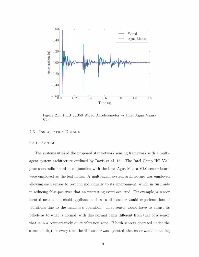
Figure 2.1 PCB 33B50 Wired Accelerometer vs Intel Agua Mansa V2.0 . . . 9
Figure 2.2 System Star Network Topography . . . . . . . . . . . . . . . . . . 10
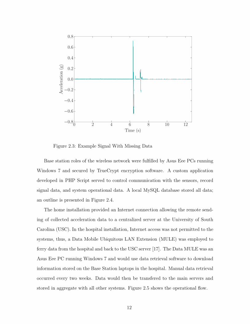
Figure 2.3 Example Signal With Missing Data . . . . . . . . . . . . . . . . . 12
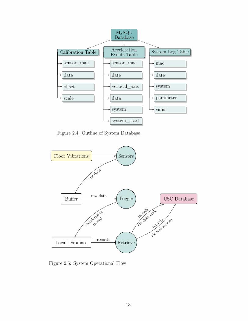
Figure 2.4 Outline of System Database . . . . . . . . . . . . . . . . . . . . . 13
Figure 2.5 System Operational Flow . . . . . . . . . . . . . . . . . . . . . . 13
Figure 2.6 Home Layout . . . . . . . . . . . . . . . . . . . . . . . . . . . . . 14
Figure 2.7 Typical Patient Room at Hospital . . . . . . . . . . . . . . . . . . 15
Figure 2.8 Accelerometer Rapid Oscillation . . . . . . . . . . . . . . . . . . . 19
Figure 2.9 Accelerometer Spike . . . . . . . . . . . . . . . . . . . . . . . . . 19
Figure 2.10 Sensor Failure Modes in a Hospital Setting for a Total of 46,214Sensor Hours . . . . . . . . . . . . . . . . . . . . . . . . . . . . . 21
Figure 2.11 Life Time of Failed Sensors in a Hospital Setting (Out of 100Sensors) . . . . . . . . . . . . . . . . . . . . . . . . . . . . . . . . 22
Figure 2.12 Home Installation’s Active Sensors . . . . . . . . . . . . . . . . . 23
Figure 2.13 Hospital Installation’s Active Sensors . . . . . . . . . . . . . . . . 23
Figure 2.14 QQ Plot for a Weibull Distribution Describing the Failure Rate . 25
Figure 2.15 QQ Plot for a Truncated Normal Distribution Describing theFailure Rate . . . . . . . . . . . . . . . . . . . . . . . . . . . . . . 26
Figure 2.16 QQ Plot for a Log-Normal Distribution Describing the Failure Rate 27
Figure 2.17 Weibull Distribution Failure Model Vs. Sensor Failures . . . . . . 28
xix

Figure 2.18 Sensor Failure Rate Bathtub Curve . . . . . . . . . . . . . . . . . 28
Figure 2.19 Home Installation’s Sensor Activations . . . . . . . . . . . . . . . 30
Figure 2.20 Home Installation’s Activity Density . . . . . . . . . . . . . . . . 31
Figure 2.21 Hospital Installation’s Sensor Activations . . . . . . . . . . . . . . 32
Figure 2.22 Hospital Installation’s Activity Density . . . . . . . . . . . . . . . 33
Figure 2.23 Home Installation’s Maximum Amplitude per Record . . . . . . . 34
Figure 2.24 Home Installation’s Signal Energy Per Record . . . . . . . . . . . 35
Figure 2.25 Home Installation’s Maximum Amplitude Vs. Signal Energy . . . 36
Figure 2.26 Hospital Installation’s Maximum Amplitude Per Record . . . . . 37
Figure 2.27 Hospital Installation’s Signal Energy Per Record . . . . . . . . . . 37
Figure 2.28 Hospital Installation’s Maximum Amplitude Vs. Signal Energy . . 38
Figure 2.29 Comparison of Hospital Reported Falls to System Captured Falls 39
Figure 2.30 Visualization of Reported Falls Vs. Captured Falls . . . . . . . . 40
Figure 2.31 Fall Event 2013-06-28 23:23:57 . . . . . . . . . . . . . . . . . . . . 42
Figure 2.32 Fall Event 2013-06-28 23:24:42 . . . . . . . . . . . . . . . . . . . . 43
Figure 2.33 Fall Event 2013-06-28 23:28:42 . . . . . . . . . . . . . . . . . . . . 43
Figure 2.34 Fall Event 2013-08-29 14:48:57 - Sensor Inside Room . . . . . . . 44
Figure 2.35 Fall Event 2013-08-29 14:48:57 - Sensor Outside Room . . . . . . 45
Figure 2.36 Fall Event 2013-11-25 17:33:49 . . . . . . . . . . . . . . . . . . . . 46
Figure 3.1 Enhanced Entity Relationship Diagram for Human Activity Database 52
Figure 4.1 Example of How to Calculate RoD . . . . . . . . . . . . . . . . . 65
Figure 4.2 Example of How to Calculate DR . . . . . . . . . . . . . . . . . . 67
xx

Figure 4.3 Signal Category Examples . . . . . . . . . . . . . . . . . . . . . . 70
Figure 4.4 Score Distribution for Linear Kernel Metric Combinations (100Trials) . . . . . . . . . . . . . . . . . . . . . . . . . . . . . . . . . 72
Figure 4.5 Score Distribution for RBF Kernel Metric Combinations (100 Trials) 73
Figure 4.6 Metric Comparison of Manually Categorized Records . . . . . . . 74
Figure 4.7 SVM Linear Kernel Metric Combination Hyperplanes . . . . . . . 76
Figure 4.8 SVM RBF Kernel Metric Combination Hyperplanes . . . . . . . . 77
Figure 4.9 SVM Classified Signal Category Examples . . . . . . . . . . . . . 78
Figure 4.10 Metric Comparison of SVM Classified Records Where DR WasUsed for Training . . . . . . . . . . . . . . . . . . . . . . . . . . . 79
Figure 4.11 Recorded Fall Events Manual Vs. SVM Categories . . . . . . . . . 80
Figure 5.1 FEEL Algorithm Process Diagram . . . . . . . . . . . . . . . . . 82
Figure 5.2 Biased Force Estimate Example . . . . . . . . . . . . . . . . . . . 87
Figure 5.3 Low-Pass FIR Filter Frequency Response . . . . . . . . . . . . . . 88
Figure 5.4 Steel Test Frame Layout . . . . . . . . . . . . . . . . . . . . . . . 90
Figure 5.5 T̂7,j for j From 1 to 3 . . . . . . . . . . . . . . . . . . . . . . . . . 91
Figure 5.6 T̂10,j for j From 1 to 3 . . . . . . . . . . . . . . . . . . . . . . . . 91
Figure 5.7 Force Estimations for an Impact on Node 7 . . . . . . . . . . . . 92
Figure 5.8 Force Estimations for an Impact on Node 10 . . . . . . . . . . . . 93
Figure 5.9 Li for an Impact on Node 7 . . . . . . . . . . . . . . . . . . . . . 94
Figure 5.10 Li for an Impact on Node 10 . . . . . . . . . . . . . . . . . . . . . 94
Figure 5.11 Steel Frame Transfer Functions . . . . . . . . . . . . . . . . . . . 96
Figure 5.12 Force Estimates by Node for an Impact on Node 2 . . . . . . . . 97
xxi

Figure 5.13 Li for an Impact on Node 2 . . . . . . . . . . . . . . . . . . . . . 98
Figure 5.14 Implementation Experimental Layout . . . . . . . . . . . . . . . . 99
Figure 5.15 Implementation Experiment Example Accelerations . . . . . . . . 101
Figure 5.16 Concrete Floor Transfer Functions . . . . . . . . . . . . . . . . . 102
Figure 5.17 Hammer Impact Force Estimations for an Impact on Location 1 . 103
Figure 5.18 Hammer Impact Li for an Impact on Location 1 . . . . . . . . . . 104
Figure 5.19 Hammer Impacts Force Magnitude Estimation Difference . . . . . 105
Figure 5.20 Hammer Impacts Force Magnitude Estimation Error . . . . . . . 105
Figure 5.21 Ball-Low Li for an Impact on Location 1 . . . . . . . . . . . . . . 106
Figure 5.22 Ball-Low Force Estimations for an Impact on Location 1 . . . . . 107
Figure 5.23 Ball-Low Force Magnitude Estimation Histogram . . . . . . . . . 108
Figure 5.24 Ball-High Li for an Impact on Location 1 . . . . . . . . . . . . . . 109
Figure 5.25 Ball-High Force Estimations for an Impact on Location 1 . . . . . 110
Figure 5.26 Ball-High Force Magnitude Estimation Histogram . . . . . . . . . 111
Figure 5.27 Bag-Low Force Estimations for an Impact on Location 2 . . . . . 112
Figure 5.28 Bag-Low Li for an Impact on Location 2 . . . . . . . . . . . . . . 113
Figure 5.29 Bag-Low Force Magnitude Estimation Histogram . . . . . . . . . 114
Figure 5.30 Bag-High Force Estimations for an Impact on Location 5 . . . . . 115
Figure 5.31 Bag-High Li for an Impact on Location 5 . . . . . . . . . . . . . . 116
Figure 5.32 Bag-High Force Magnitude Estimation Histogram . . . . . . . . . 116
Figure 5.33 D-Jump Force Estimations for an Impact on Location 1 . . . . . . 118
Figure 5.34 D-Jump Li for an Impact on Location 1 . . . . . . . . . . . . . . 119
Figure 5.35 D-Jump Force Magnitude Estimation Histogram . . . . . . . . . . 119
xxii

Figure 5.36 J-Jump Li for an Impact on Location 3 . . . . . . . . . . . . . . . 120
Figure 5.37 J-Jump Force Estimations for an Impact on Location 3 . . . . . . 121
Figure 5.38 J-Jump Force Magnitude Estimation Histogram . . . . . . . . . . 122
Figure 5.39 W-Jump Force Estimations for an Impact on Location 4 . . . . . 123
Figure 5.40 W-Jump Li for an Impact on Location 4 . . . . . . . . . . . . . . 124
Figure 5.41 W-Jump Force Estimation Histogram . . . . . . . . . . . . . . . . 125
Figure 5.42 Force Magnitude Estimation Difference for Concrete Floor Im-pacts Using Data Downsampled to 400 Hz . . . . . . . . . . . . . 127
Figure 5.43 Force Magnitude Estimation Error for Concrete Floor ImpactsUsing Data Downsampled to 400 Hz . . . . . . . . . . . . . . . . . 127
Figure 5.44 Force Magnitude Estimation for Concrete Floor Impacts UsingData Upsampled From 400 Hz to 1651.7 Hz . . . . . . . . . . . . . 129
Figure 5.45 orce Magnitude Estimation Error for Concrete Floor ImpactsUsing Data Upsampled From 400 Hz to 1651.7 Hz . . . . . . . . . 129
Figure 5.46 Concrete Floor Retest Experiment Example Accelerations . . . . 131
Figure 5.47 Difference Between Force Magnitude Estimation And MeasuredHammer Force for Implementation Retest Experiment . . . . . . 133
Figure 5.48 Error Between Force Magnitude Estimation And Measured Ham-mer Force for Implementation Retest Experiment . . . . . . . . . 133
Figure 6.1 EFFECT Pedagogical Structure [49, 50, 51] . . . . . . . . . . . . 138
Figure 6.2 EFFECT Developmental Structure [55] . . . . . . . . . . . . . . . 139
Figure 6.3 Distribution of Responses Broken Down by Students’ ExpectedGrade for Question 3 “Indicate How Conducive to Learning TheFollowing Course Activities Were” . . . . . . . . . . . . . . . . . . 146
Figure 6.4 Distribution of Responses Broken Down by Students’ ExpectedGrade for Question 6.a “Did The Lab Visit Make The Connec-tion Between Math and Physics Easier to Understand?” . . . . . 147
xxiii
Figure 6.5 Distribution of Responses Broken Down by Students’ ExpectedGrade for Question 4 “How Confident Do You Feel About TheFollowing Topics?” . . . . . . . . . . . . . . . . . . . . . . . . . . 149
Figure B.1 Fall Event 2013-06-17 21:57:19 | Sensor D4E1 . . . . . . . . . . . 168
Figure B.2 Fall Event 2013-06-17 21:57:19 | Sensor B3B0 . . . . . . . . . . . 169
Figure B.3 Fall Event 2013-06-17 21:58:54 | Sensor BB46 . . . . . . . . . . . 169
Figure B.4 Fall Event 2013-06-17 21:58:54 | Sensor BB87 . . . . . . . . . . . 170
Figure B.5 Fall Event 2013-06-17 22:03:19 | Sensor BB87 . . . . . . . . . . . 170
Figure B.6 Fall Event 2013-06-17 22:10:07 | Sensor BB87 . . . . . . . . . . . 171
Figure B.7 Fall Event 2013-06-20 17:14:23 | Sensor D4E1 . . . . . . . . . . . 172
Figure B.8 Fall Event 2013-06-20 17:14:23 | Sensor BB46 . . . . . . . . . . . 172
Figure B.9 Fall Event 2013-06-28 23:23:57 | Sensor 8D2C . . . . . . . . . . . 173
Figure B.10 Fall Event 2013-06-28 23:24:42 | Sensor 8D2C . . . . . . . . . . . 173
Figure B.11 Fall Event 2013-06-28 23:28:42 | Sensor 8D2C . . . . . . . . . . . 174
Figure B.12 Fall Event 2013-06-28 23:30:38 | Sensor 8D2C . . . . . . . . . . . 174
Figure B.13 Fall Event 2013-07-25 17:49:29 | Sensor B3A1 . . . . . . . . . . . 175
Figure B.14 Fall Event 2013-07-25 17:49:29 | Sensor BB7E . . . . . . . . . . . 175
Figure B.15 Fall Event 2013-07-30 04:45:49 | Sensor BB48 . . . . . . . . . . . 176
Figure B.16 Fall Event 2013-08-27 10:58:35 | Sensor BB48 . . . . . . . . . . . 177
Figure B.17 Fall Event 2013-08-27 10:58:35 | Sensor E0A8 . . . . . . . . . . . 177
Figure B.18 Fall Event 2013-08-27 10:58:35 | Sensor E7EC . . . . . . . . . . . 178
Figure B.19 Fall Event 2013-08-27 10:58:35 | Sensor 3496 . . . . . . . . . . . . 178
Figure B.20 Fall Event 2013-08-29 14:48:57 | Sensor E7DB . . . . . . . . . . . 179
xxiv

Figure B.21 Fall Event 2013-08-29 14:48:57 | Sensor 3493 . . . . . . . . . . . . 179
Figure B.22 Fall Event 2013-08-31 18:07:07 | Sensor B3A5 . . . . . . . . . . . 180
Figure B.23 Fall Event 2013-08-31 18:07:07 | Sensor E7DB . . . . . . . . . . . 180
Figure B.24 Fall Event 2013-08-31 18:07:07 | Sensor 8D2C . . . . . . . . . . . 181
Figure B.25 Fall Event 2013-09-22 02:45:21 | Sensor C7AE . . . . . . . . . . . 182
Figure B.26 Fall Event 2013-09-22 02:45:21 | Sensor DC67 . . . . . . . . . . . 182
Figure B.27 Fall Event 2013-09-22 02:45:21 | Sensor 2E73 . . . . . . . . . . . . 183
Figure B.28 Fall Event 2013-10-03 12:34:31 | Sensor B3A5 . . . . . . . . . . . 184
Figure B.29 Fall Event 2013-10-22 20:02:20 | Sensor E7EC . . . . . . . . . . . 185
Figure B.30 Fall Event 2013-10-26 07:34:28 | Sensor E7EC . . . . . . . . . . . 186
Figure B.31 Fall Event 2013-10-28 23:25:33 | Sensor E0A8 . . . . . . . . . . . 187
Figure B.32 Fall Event 2013-11-25 17:33:49 | Sensor B3A5 . . . . . . . . . . . 188
Figure B.33 Fall Event 2013-11-25 17:33:49 | Sensor BB7C . . . . . . . . . . . 188
Figure B.34 Fall Event 2013-11-25 17:33:49 | Sensor 3087 . . . . . . . . . . . . 189
Figure B.35 Fall Event 2013-11-25 17:33:49 | Sensor 3493 . . . . . . . . . . . . 189
Figure B.36 Fall Event 2013-12-03 03:47:22 | Sensor B3A5 . . . . . . . . . . . 190
Figure B.37 Fall Event 2013-12-09 04:59:04 | Sensor B3A5 . . . . . . . . . . . 191
Figure B.38 Fall Event 2013-12-09 04:59:04 | Sensor BB45 . . . . . . . . . . . 191
Figure B.39 Fall Event 2013-12-09 04:59:04 | Sensor 8D2C . . . . . . . . . . . 192
Figure B.40 Fall Event 2013-12-09 04:59:04 | Sensor 8F1E . . . . . . . . . . . 192
Figure D.1 SVM 3rd Degree Polynomial Kernel Metric Combination Hy-perplanes . . . . . . . . . . . . . . . . . . . . . . . . . . . . . . . 204
xxv

Figure D.2 Score Distribution for 3rd Degree Polynomial Kernel MetricCombinations (100 Trials) . . . . . . . . . . . . . . . . . . . . . . 205
Figure E.1 Score Distribution for Sigmoid Kernel Metric Combinations (100Trials) . . . . . . . . . . . . . . . . . . . . . . . . . . . . . . . . . 208
Figure H.1 Force Estimates by Node for an Impact on Node 3 . . . . . . . . 231
Figure H.2 Li for an Impact on Node 3 . . . . . . . . . . . . . . . . . . . . . 231
Figure H.3 Force Estimates by Node for an Impact on Node 6 . . . . . . . . 233
Figure H.4 Li for an Impact on Node 6 . . . . . . . . . . . . . . . . . . . . . 233
Figure H.5 Force Estimates by Node for an Impact on Node 7 . . . . . . . . 235
Figure H.6 Li for an Impact on Node 7 . . . . . . . . . . . . . . . . . . . . . 235
Figure H.7 Force Estimates by Node for an Impact on Node 10 . . . . . . . . 237
Figure H.8 Li for an Impact on Node 10 . . . . . . . . . . . . . . . . . . . . . 237
Figure H.9 Force Estimates by Node for an Impact on Node 11 . . . . . . . . 239
Figure H.10 Li for an Impact on Node 11 . . . . . . . . . . . . . . . . . . . . . 239
Figure H.11 Force Estimates By Node for An Impact On Node 14 . . . . . . . 241
Figure H.12 Li for an Impact on Node 14 . . . . . . . . . . . . . . . . . . . . . 241
Figure H.13 Force Estimates by Node for an Impact on Node 15 . . . . . . . . 243
Figure H.14 Li for an Impact on Node 15 . . . . . . . . . . . . . . . . . . . . . 243
Figure I.1 Hammer Impact Force Estimations for an Impact on Location 2 . 245
Figure I.2 Hammer Impact Li for an Impact on Location 2 . . . . . . . . . . 246
Figure I.3 Hammer on Location 2 Accelerations . . . . . . . . . . . . . . . . 246
Figure I.4 Hammer Impact Force Estimations for an Impact on Location 3 . 247
xxvi

Figure I.5 Hammer Impact Li for an Impact on Location 3 . . . . . . . . . . 248
Figure I.6 Hammer on Location 3 Accelerations . . . . . . . . . . . . . . . . 248
Figure I.7 Hammer Impact Force Estimations for an Impact on Location 4 . 249
Figure I.8 Hammer Impact Li for an Impact on Location 4 . . . . . . . . . . 250
Figure I.9 Hammer on Location 4 Accelerations . . . . . . . . . . . . . . . . 250
Figure I.10 Hammer Impact Force Estimations for an Impact on Location 5 . 251
Figure I.11 Hammer Impact Li for an Impact on Location 5 . . . . . . . . . . 252
Figure I.12 Hammer on Location 5 Accelerations . . . . . . . . . . . . . . . . 252
xxvii

List of Symbols
Amax maximum value of amplitude present in a signal
Es signal energy in a signal processing sense
FSnew new sampling rate
FSold original sampling rate
∆ (accelerometer unit conversion) offset value;
(RoD) window shift
∆t signal delay time
Γ raw 1 g value for the sensor axis
Γ−1 the last calculated raw 1 g value for the sensor axis
αi regularization parameter in the range of 0 ≤ αi ≤C
γ (SVM) shape parameter;
(Weibull distribution) scale parameter
F̂ force magnitude estimation for an acceleration event
F̂i,j force magnitude estimation for the i-th location and j-sensor
L̂ coefficient which indicates the impact’s location
λ failure rate[F̂i,j
]matrix containing force estimations for the i-th locations and j-
sensors
Pxx(f) power spectral density of x
Pxy(f) power spectral density of x to y
Pyx(f) power spectral density of y to x
Pyy(f) power spectral density of y
T̂(f) transfer function estimate
xxviii

µ mean
ρ independent intercept parameter
ρnan density of NaN present in a signal
ρxy Pearson product-moment correlation coefficient
σ standard deviation
σ‡ vector of standard deviations
τ offset integer
τF̂i,jdata point in the signal of the peak in the force estimate
τF̂i,jdata point in the signal of the peak in the force estimate
{Li} vector of location coefficients
{F̂i,j} force estimation vector for the i-th location and j-sensor
no number of overlapping points per window
ns number of points present in a signal
nw number of points per window
nnan number of NaN present in a signal
x′ training data
yi vector of the form y ∈ {−1, 1}n
yi,g i-th accelerometer value in units of gravity
yi,raw i-th raw value (i.e. before conversion to gravity units) read from the
accelerometer
C (accelerometer unit conversion) scale value for an accelerometer axis;
(SVM) penalty parameter
D signal sorted in descending order
d signal delay
f number of failures
xxix

i (FEEL) location;
(MADr) index of signal;
(RoD) point in acceleration signal
j (FEEL) sensor;
(RoD) window adjusting integer
K support vector machine kernel function
k (Weibull distribution) shape parameter;
(deviation method) point in[F̂i,j
]being compared
N number of coefficients in the filter
n (event localization) number of points in window;
(signal energy) last time step;
(SVM) number of points of x
S detrended acceleration signal
T sensor acceleration trigger threshold
t (log-normal distribution) time value of interest;
(normal distribution) time value of interest;
(reliability) time period that failures f occurred in;
(signal processing) time;
(Weibull distribution) time value of interest
x (SVM) testing data or data to be classified;
(FEEL) force input
y acceleration output
xxx

List of Abbreviations
ABET . . . . . . . . . . . . . . . . . . . . . . . Accreditation Board for Engineering and Technology
ASCE . . . . . . . . . . . . . . . . . . . . . . . . . . . . . . . . . . . . . . . . American Society of Civil Engineers
COV . . . . . . . . . . . . . . . . . . . . . . . . . . . . . . . . . . . . . . . . . . . . . . . . . . . . . . . . . . . . . . . . . . Covariance
DAQ . . . . . . . . . . . . . . . . . . . . . . . . . . . . . . . . . . . . . . . . . . . . . . . . . . . . Data Acquisition System
DOM . . . . . . . . . . . . . . . . . . . . . . . . . . . . . . . . . . . . . . . . . . . . . . . . . . . . . . . Drawn Over Mandrel
DR . . . . . . . . . . . . . . . . . . . . . . . . . . . . . . . . . . . . . . . . . . . . . . . . . . . . . . . . . . . . . . Dispersion Ratio
EFFECT. . . . . . . . . . . . . . . . . .Environments For Fostering Effective Critical Thinking
FEEL . . . . . . . . . . . . . . . . . . . . . . . . Force Estimation and Event Localization Algorithm
FFT . . . . . . . . . . . . . . . . . . . . . . . . . . . . . . . . . . . . . . . . . . . . . . . . . . . . . . Fast Fourier Transform
FIR. . . . . . . . . . . . . . . . . . . . . . . . . . . . . . . . . . . . . . . . . . . . . . . . . . . . . .Finite Impulse Response
IFFT . . . . . . . . . . . . . . . . . . . . . . . . . . . . . . . . . . . . . . . . . . . . . . Inverse Fast Fourier Transform
LAN . . . . . . . . . . . . . . . . . . . . . . . . . . . . . . . . . . . . . . . . . . . . . . . . . . . . . . . . . Local Area Network
MAC . . . . . . . . . . . . . . . . . . . . . . . . . . . . . . . . . . . . . . . . . . . . . . . . . . Modal Assurance Criterion
MAC Address . . . . . . . . . . . . . . . . . . . . . . . . . . . . . . . . . . . . . . Media Access Control Address
MAD. . . . . . . . . . . . . . . . . . . . . . . . . . . . . . . . . . . . . . . . . . . . .Maximum Amplitude Difference
MADr. . . . . . . . . . . . . . . . . . . . . . . . . . . . . . . . . . . . . .Maximum Amplitude Difference Ratio
MTBF . . . . . . . . . . . . . . . . . . . . . . . . . . . . . . . . . . . . . . . . . . . . . . . Mean Time Between Failure
xxxi

MTTF . . . . . . . . . . . . . . . . . . . . . . . . . . . . . . . . . . . . . . . . . . . . . . . . . . . . . Mean Time To Failure
MULE . . . . . . . . . . . . . . . . . . . . . . . . . . . . . . . . . . . . . . . . . Mobile Ubiquitous LAN Extension
NaN . . . . . . . . . . . . . . . . . . . . . . . . . . . . . . . . . . . . . . . . . . . . . . . . . . . . . . . . . . . . . . . Not a Number
PC. . . . . . . . . . . . . . . . . . . . . . . . . . . . . . . . . . . . . . . . . . . . . . . . . . . . . . . . . . . .Personal Computer
PH . . . . . . . . . . . . . . . . . . . . . . . . . . . . . . . . . . . . . . . . . . . . . . . . . . . . . Palmetto Health Hospital
QQ. . . . . . . . . . . . . . . . . . . . . . . . . . . . . . . . . . . . . . . . . . . . . . . . . . . . . . . . . . . . .Quantile-Quantile
RBF . . . . . . . . . . . . . . . . . . . . . . . . . . . . . . . . . . . . . . . . . . . . . . . . . . . . . . . Radial Basis Function
RoD . . . . . . . . . . . . . . . . . . . . . . . . . . . . . . . . . . . . . . . . . . . . . . . . . . . . . . . . . . . Rate of Dispersion
SDII . . . . . . . . . . . . . . . Structural Dynamics and Intelligent Infrastructure Laboratory
SDOF. . . . . . . . . . . . . . . . . . . . . . . . . . . . . . . . . . . . . . . . . . . . . . . . . . .Single Degree of Freedom
SVM. . . . . . . . . . . . . . . . . . . . . . . . . . . . . . . . . . . . . . . . . . . . . . . . . . . . . Support Vector Machine
UDP. . . . . . . . . . . . . . . . . . . . . . . . . . . . . . . . . . . . . . . . . . . . . . . . . . . . .User Datagram Protocol
US . . . . . . . . . . . . . . . . . . . . . . . . . . . . . . . . . . . . . . . . . . . . . . . . . . . . . . United States of America
USB . . . . . . . . . . . . . . . . . . . . . . . . . . . . . . . . . . . . . . . . . . . . . . . . . . . . . . . . . Universal Serial Bus
USC . . . . . . . . . . . . . . . . . . . . . . . . . . . . . . . . . . . . . . . . . . . . . . . . . University of South Carolina
VAMC. . . .William Jennings Bryan Dorn Veteran’s Administration Medical Center
xxxii

Chapter 1
Introduction
1.1 Motivation
In the US alone, 20% of citizens will be over the age of 65 by the year 2030 [2]; the
largest challenge facing this growing demographic is not a new disease but a simple
motion - the fall. These events are the premier cause of fatal and nonfatal injuries
[2, 3, 4], and hospital trauma admissions among older adults [2]. They affect one in
three age 65+ every year [2, 4] and over half of those age 80+ [4]. In fact, a fall is so
common that every 17 seconds an older adult is treated for fall-related injuries, and
every 30 minutes, an older adult dies from fall complications [3].
This accounts for “25% of all hospital admissions and 40% of all nursing home
admissions” [4]. Of the population admitted, “40% [...] do not return to independent
living [and] 25% die within a year” [4]. That means 65% of those experiencing a fall
cannot return to their previous quality of independent living.
Costs stemming from falls are high. Direct medical costs “adjusted for inflation,
were $30 billion” in 2012 with an expected increase of annual direct and indirect costs
to $67.7 billion (in 2012 dollars) by the year 2020 [3].
The expense does not stop there but further continues to the health impact on
the person who fell. Moderate to severe injuries can result from an incident. These
include “lacerations, hip fractures, and head traumas” which “can make it hard to
get around or live independently, and increase the risk of early death” [2].
Even though only 20-30% of falls result in moderate to severe injuries [2], “a
1

large percentage of non-injured fallers (47%) cannot get up without assistance” [4].
The time spent immobile directly affects the person’s health outcome. Within 30-
60 minutes of compression from a fall, muscle cells begin to breakdown potentially
resulting in dehydration, pressure sores, hypothermia, and pneumonia [4].
Thus, the outcome of a fall becomes dependent upon the immediate response and
rescue of those immobile persons [5, 6]. Help after an immobilizing fall increases
survival rates by 80% and the probability for the person to return to independent
living [4]. If one could largely reduce response time, more older adults could return to
their residences in a healthy state rather than sacrifice their individual independence.
Rapid response would decrease the medical costs associated with falls, along with the
amount of nursing home admissions, and more importantly, the amount of fatalities
due to falls.
Those who fall can develop a fear of falling, even if no injuries were sustained.
The person may be driven by this fear to limit their activity. Risk of falling conse-
quently increases because of the person’s reduced mobility and physical fitness [2, 3].
Several health problems are associated with impaired mobility “including depression,
cardiovascular disease, cancer, and injuries secondary to falls and automobile crashes”
[2]. Fear can tug at the person’s mind, causing “feelings of helplessness and social
isolation” to further complicate one’s health state [3].
Combating falls is harder than prevention techniques alone. Restraints have been
used to restrict a patient’s movements in an effort to reduce the chance of falling.
However, forcefully limiting movement has a similar outcome as the patient voluntar-
ily limiting his activity due to fear. It does not work. Muscles weaken and physical
function declines which increases the falling risk rather than reduce it [3]. Prevention
must be done in ways that do not restrict mobility, but the chance of falling remains
because every movement has that potential implicitly.
2

1.2 Current State of Fall Detection Technology
The ever present fall risk directs development towards methods other than pre-
vention. Commercial solutions utilizing worn pendants, like Life Alert, remove the
need to be near a phone to call for aid after a fall event. Effectiveness of the system
shows when a Life Alert member goes to a retirement home, members go “six years
later than an equivalent aged senior” [7]. The system also impacts mental health as
87% of Life Alert users say the protection provided is a main or important factor in
the decision to stay at home [7]. However, the system is still limited because of user
dependence. Users need to be conscious to press the pendant and need to be wearing
the pendant in the first place.
Computer vision techniques with machine learning have been used successfully to
92% accuracy when using simulated falls by able-bodied participants in home envi-
ronments [8]. Visual techniques are computationally intensive and intrusive, bringing
concerns of processing power and user privacy. The machine-learning component
when applied to human activity (i.e. a person’s normal schedule) has the possibility
to predict a fall and could be used as part of a preemptive measure.
An alternative to using cameras is to use infrared technology which is somewhat
less privacy-intrusive [9]. However, household residents’ perception is one of “being
watched” so the privacy concern persists [5]. The system utilized was based on user
activity and was only 35.7% successful in detection [9]. They described falls that
required aid as those where the observed was inactive. Challenges arise as aid may
be required in situations where the observed is not completely inactive. For instance,
one can break a hip and crawl across the floor in an effort to get to a phone, but in
the end the phone is out of reach because the person cannot get up to reach it. The
observed in this case needs medical assistance, but by the concept presented, this
person would not receive aid.
Worn accelerometers have been suggested as a good way to differentiate between
3

human activities. Rybina et al correctly identified hopping, jumping, and skipping in
all cases, running and balancing in 11 out of 12 cases using the Time Domain Correla-
tion Coefficient in a laboratory setting [10]. Other research suggests the method used
has a medium/high uncertainty without time synchronization, making it not ideal
for fall detection [11]. Another worn accelerometer method using a Hidden Markov
Model successfully detected 68 of 74 human falls in laboratory testing [12]. While
privacy issues dissipate using acceleration data, other challenges arise from wearing
devices. The assumption that the device remains in a fixed position to the wearer
does not fully account for devices moving around during human activities. More
importantly, compliance issues abound as “patients have low will to wear devices
for detecting falls because they feel well before a fall occurs” or consider the device
intrusive [6].
The previous directs research towards a less intrusive solution. Floor vibrations
have been previously proposed as a way to detect falls, and dummies were used for
laboratory testing of the algorithms [5, 13]. One team developed and patented a
special device for use in fall detection [5]. However, little information is publicly
available to determine the effectiveness of this device.
Techniques presented by Zigel et al added microphones as an additional input
to recognize a fall [13]. However, energy methods were employed, which presents
challenges if the event is near or far from a sensor. Different transient wave forms
can produce the same amount of energy and lead to incorrect identification or missed
events. Damping ratios are often assumed by the spectrum employed by Zigel et al,
opening the possibility of further error as the characteristics of the structure are not
fully realized [14].
4

1.3 What’s Next?
The author seeks to overcome the challenges of other methods towards the ideal
human-induced vibration monitoring system. We begin this journey by describing
what the ideal system would be:
(1) user-independent to remove the need for any specific user information or userinput;
(2) environmentally-based, removing the need for the user to wear any devices andthe challenges associated with worn devices;
(3) able to operate on devices that are naturally unobtrusive;
(4) privacy respecting;
(5) inexpensive to operate and maintain, both monetarily and computationally;
(6) and adaptive to any environment (e.g. registers event regardless of distancefrom event to sensor).
This ideal can be extended when one looks at human fall detection from the angle
of structural vibrations for a potential product implementation. The system should
additionally seek to:
(1) not require modifications to the structure;
(2) not require modifications to the electrical network of the buildings;
(3) not interfere with normal network operation in the building;
(4) and easy to install.
The natural sensor choice for the ideal system is a wireless smart accelerometer.
These sensors are small and can be easily attached anywhere on a structure, allowing
them to be unobtrusive whilst monitoring the environment of the user. They are
typically inexpensive to operate and maintain (e.g. smart phones often come equipped
with an accelerometer), and can perform some analytics on their own. No structural
or electrical modifications of the building are needed.
5

This work utilizes wireless accelerometers to design and implement a human-
induced vibration monitoring system towards the end goal of developing the ideal
human fall detection system. Systems are installed in two different real world en-
vironments - a hospital and a private family residence - resulting in the capture of
several fall events. The information is cared for according to a data management
plan based with a relational database design to provide flexibility for the future as
research progresses.
A human fall detection system using structural vibrations would require the ability
for the system to sort good from bad signals, ideally on the sensor level. Signal se-
lection as a preprocessing operation, reduces the amount of information for detection
algorithms to work through making the system as a whole more efficient. Methods
for using machine learning through Support Vector Machine (SVM) with new signal
metrics are developed to enable individual sensors to decide signal quality.
The challenge after initial signal selection thus becomes detecting an impact from
a human fall. Acceleration amplitudes the sensor experiences will vary based on the
distance between a sensor and an impact. Thus any algorithm for fall detection based
in vibrations has to overcome distance to be effective, and ideally would not require
time synchronization or estimate structural properties whilst doing so. This led to
the development of the Force Estimation and Event Localization Algorithm (FEEL)
which accomplishes all those goals and is additionally designed to scale with any
number of sensors, which increases the robustness of the system.
FEEL utilizes the frequency domain as part of relating accelerations to a force and
location. The concept of frequency domain can be hard to grasp, leading the author
to include an education module for teaching the concept. The Environments For
Fostering Effective Critical Thinking (EFFECT) framework was chosen for creating
the module due to the focus on critical thinking and increasing knowledge transfer,
whilst encouraging the student to improve other beneficial professional skills.
6

Chapter 2
System Design and Implementation
2.1 Introduction
A robust, automated system must be designed for deployment in the real world
in order to learn more about human activity through vibrations. The system should
emulate the ideals for a human fall detection system as outlined in Section 1.3, so that
the system may operate in diverse environments. In a hospital environment like that
of William Jennings Bryan Dorn Veteran’s Administration Medical Center (VAMC),
the additional implementation requirements of the system are very important due to
the nature of hospital equipment. The VAMC has numerous networks running and
machines operating on various frequency bands that a monitoring system, not being
aware of this fact, could interfere with and affect the normal health care operations
of the hospital. For the case of private residences, an owner would not necessarily
want to alter his home nor have installation personnel spending a large amount of
time interrupting his day.
Initial research into a system was conducted by Davis et al [15], and is where the
ultimate system design draws its basis. Various network configurations employing
wireless accelerometers were explored, ultimately resulting in an adaptive network
that allows the capturing of human-induced vibrations within the bounds of the ideal
system. This work puts forth a standard for all human activity monitoring systems
that has been vetted through installations at both VAMC and a private residence.
The goal for developing this system focused on capturing real world fall events
7

through structural vibrations, with many human falls being captured during the
study period. Several fall events are showcased with discussion relating what is seen
in the acceleration plots to that of the reported incidents’ descriptions, showing the
possibility of fall detection through structural vibrations. In addition, the author
explores features of the signals and vibration activity trends that closely match the
general schedule of the people at each installation location which can lead to broader
human activity monitoring for other health care applications.
2.2 Wireless Accelerometer Validation
Before any system was installed, the wireless accelerometer on the Intel Agua
Mansa V2.0 sensor board needed to be validated as operating to the wired accelerom-
eter standard. The two accelerometers were sitting side by side on a steel frame table,
where a tennis ball was dropped and allowed to come to rest on the table. A NI-9234
DAQ operated a PCB Piezotronics 333B50 accelerometer with 1019 mV/g collecting
data at 1651.7 Hz for the wired accelerometer standard. Data was collected for both
accelerometers simultaneously as the ball bounced on the table. Time vectors were
generated for each signal with the Agua Mansa’s time vector being adjusted until a
match was obtained between the two signals. The Agua Mansa accelerometer was
found to be operating at approximately 316 Hz and matching the wired accelerome-
ter very well as seen in Figure 2.1. Differences in amplitude are due to the sensors
having two different sampling rates, which causes the sensors to see different parts of
the waveform.
The experiment was repeated using another Agua Mansa sensor, with the results
being the same as the first trial. Thus the remainder of the sensors are considered to
be operating at the same rate.
8
0.0 0.2 0.4 0.6 0.8 1.0 1.2Time (s)
-0.60
-0.40
-0.20
0.00
0.20
0.40
0.60
Acce
lerat
ion
(g)
WiredAgua Mansa
Figure 2.1: PCB 33B50 Wired Accelerometer vs Intel Agua MansaV2.0
2.3 Installation Details
2.3.1 System
The systems utilized the proposed star network sensing framework with a multi-
agent system architecture outlined by Davis et al [15]. The Intel Camp Hill V2.1
processor/radio board in conjunction with the Intel Agua Mansa V2.0 sensor board
were employed as the leaf nodes. A multi-agent system architecture was employed
allowing each sensor to respond individually to its environment, which in turn aids
in reducing false-positives that an interesting event occurred. For example, a sensor
located near a household appliance such as a dishwasher would experience lots of
vibrations due to the machine’s operation. That sensor would have to adjust its
beliefs as to what is normal, with this normal being different from that of a sensor
that is in a comparatively quiet vibration zone. If both sensors operated under the
same beliefs, then every time the dishwasher was operated, the sensor would be telling
9
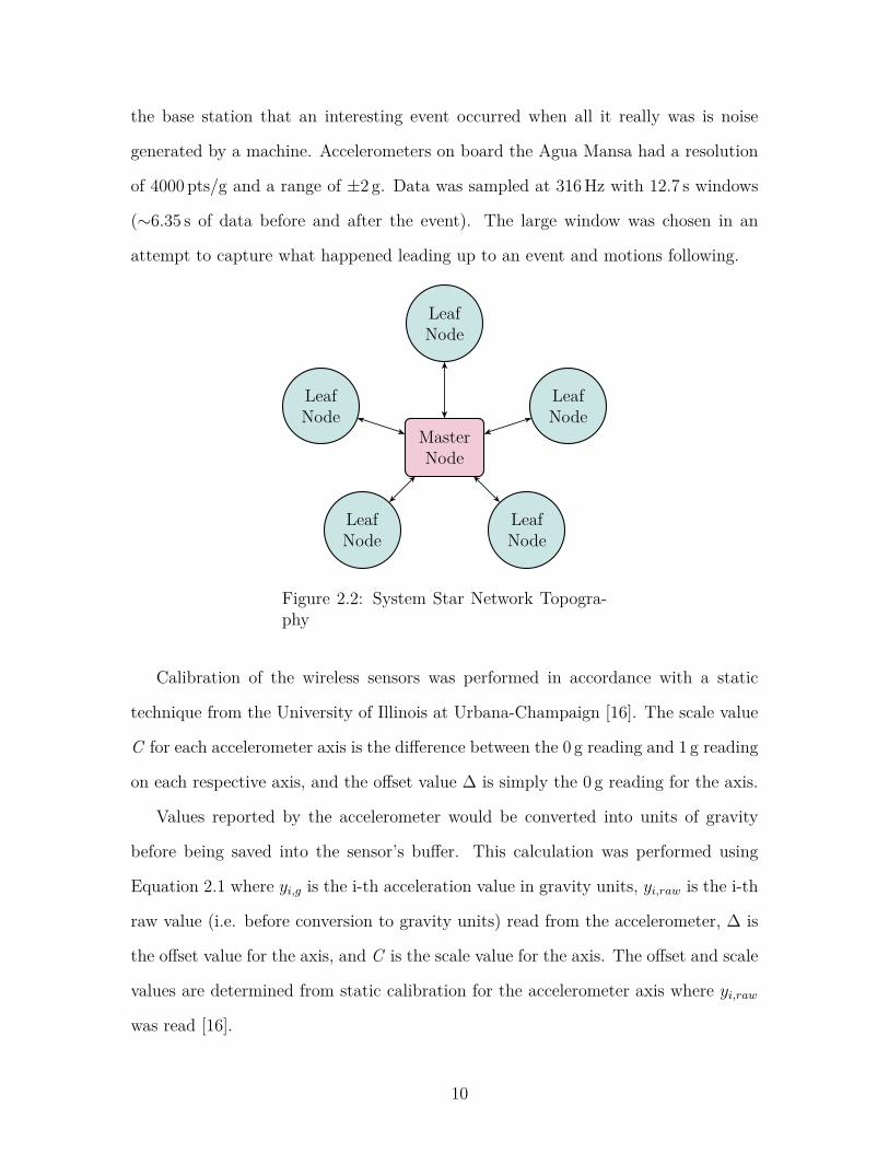
the base station that an interesting event occurred when all it really was is noise
generated by a machine. Accelerometers on board the Agua Mansa had a resolution
of 4000 pts/g and a range of ±2 g. Data was sampled at 316 Hz with 12.7 s windows
(∼6.35 s of data before and after the event). The large window was chosen in an
attempt to capture what happened leading up to an event and motions following.
MasterNode
LeafNode
LeafNode
LeafNode
LeafNode
LeafNode
Figure 2.2: System Star Network Topogra-phy
Calibration of the wireless sensors was performed in accordance with a static
technique from the University of Illinois at Urbana-Champaign [16]. The scale value
C for each accelerometer axis is the difference between the 0 g reading and 1 g reading
on each respective axis, and the offset value ∆ is simply the 0 g reading for the axis.
Values reported by the accelerometer would be converted into units of gravity
before being saved into the sensor’s buffer. This calculation was performed using
Equation 2.1 where yi,g is the i-th acceleration value in gravity units, yi,raw is the i-th
raw value (i.e. before conversion to gravity units) read from the accelerometer, ∆ is
the offset value for the axis, and C is the scale value for the axis. The offset and scale
values are determined from static calibration for the accelerometer axis where yi,raw
was read [16].
10

yi,g = yi,raw − ∆C
(2.1)
A threshold level of ±50 pts (typically 0.0125 g) served to indicate a vibration
event of note (threshold choice discussed more in Section 2.4). The system is triggered
if the condition presented in Equation 2.2 where Γ is the raw 1 g value for the sensor
axis, yi,raw is the current (or i-th) raw value read from the accelerometer on the axis,
and T is the threshold for the axis.
|Γ − yi,raw| ≥ T (2.2)
The value of Γ for each sensor axis changes depending on the orientation of the
sensor. Initially, Γ is determined by filling up the sensor’s buffer once under “at rest”
conditions, and then taking the average of those values. Each time a new value is
read from the accelerometer, Γ updates using a version of a running average seen in
Equation 2.3 where Γ raw 1 g value for the sensor axis, Γ−1 is the last calculated raw
1 g value for the sensor axis, and yi,raw is the i-th raw value (i.e. before conversion to
gravity units) read from the accelerometer.
Γ = Γ−1 · yi,raw
2 (2.3)
Each leaf node streamed data over an User Datagram Protocol (UDP) wireless
local area network connection provided by the base station computer where all pro-
cessing was handled, including buffering, triggering, and local storage. UDP con-
nections, by its nature, sometimes lose data when communicating between entities
leaving gaps in the signal (see Figure 2.3). The platform combats this by adding in
synchronization packages that allow for tracking how many data points should have
been seen, that way the unreliable nature of UDP connections can be overcome.
11
0 2 4 6 8 10 12Time (s)
−0.8
−0.6
−0.4
−0.2
0.0
0.2
0.4
0.6
0.8
Acce
lerat
ion
(g)
Figure 2.3: Example Signal With Missing Data
Base station roles of the wireless network were fulfilled by Asus Eee PCs running
Windows 7 and secured by TrueCrypt encryption software. A custom application
developed in PHP Script served to control communication with the sensors, record
signal data, and system operational data. A local MySQL database stored all data;
an outline is presented in Figure 2.4.
The home installation provided an Internet connection allowing the remote send-
ing of collected acceleration data to a centralized server at the University of South
Carolina (USC). In the hospital installation, Internet access was not permitted to the
systems, thus, a Data Mobile Ubiquitous LAN Extension (MULE) was employed to
ferry data from the hospital and back to the USC server [17]. The Data MULE was an
Asus Eee PC running Windows 7 and would use data retrieval software to download
information stored on the Base Station laptops in the hospital. Manual data retrieval
occurred every two weeks. Data would then be transfered to the main servers and
stored in aggregate with all other systems. Figure 2.5 shows the operational flow.
12
MySQLDatabase
Calibration Table AccelerationEvents Table System Log Table
sensor_mac
date
offset
scale
sensor_mac
date
vertical_axis
data
system
system_start
mac
date
system
parameter
value
Figure 2.4: Outline of System Database
Floor Vibrations Sensors
Buffer Trigger USC Database
Local Database Retrieve
rawdata
raw data
accele
ration
record
records
record
s
viadata
mule
record
s
viaweb
servic
e
Figure 2.5: System Operational Flow
13

2.3.2 Home Environment
The home installation occurred on the first story of a two story wood-framed
house located in Columbia, South Carolina. A family of four resided there, including
two identical twin toddlers 2.5 years of age. Sensors were installed in the living room
of the home, a location chosen for its high human activity. Sensors were attached to
hardwood floors using double-sided duct tape. Figure 2.6 provides a diagram of the
home installation.
Kitchen
Dining
Bathroom
Mas
ter
Bedr
oom
Clo
set
Couch
TV
ChairChair
Sensor
Sens
or
475 cm
406c
m92
cm13
5cm
205 cm135 cm 135 cm
Figure 2.6: Home Layout
2.3.3 Hospital Environment
Systems were installed on the fourth floor of the hospital whose flooring was
vinyl layered on top of reinforced concrete. The particular wing monitored contained
14
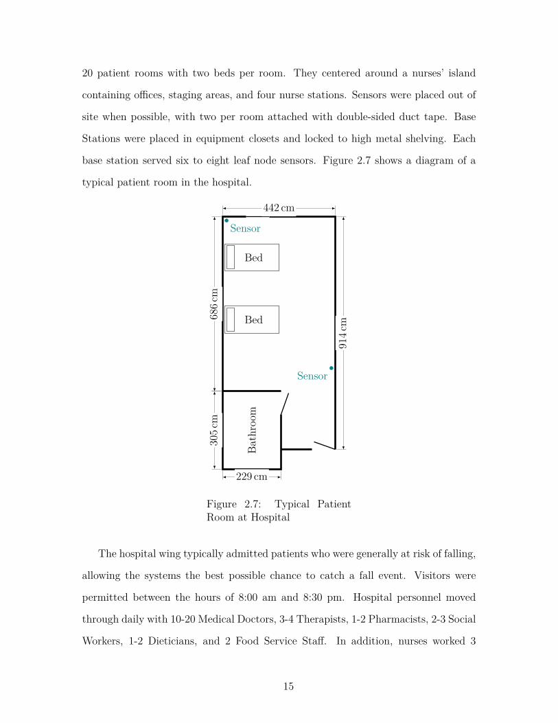
20 patient rooms with two beds per room. They centered around a nurses’ island
containing offices, staging areas, and four nurse stations. Sensors were placed out of
site when possible, with two per room attached with double-sided duct tape. Base
Stations were placed in equipment closets and locked to high metal shelving. Each
base station served six to eight leaf node sensors. Figure 2.7 shows a diagram of a
typical patient room in the hospital.
Bath
room
Bed
Bed
Sensor
Sensor
442 cm
914c
m
229 cm
305c
m68
6cm
Figure 2.7: Typical PatientRoom at Hospital
The hospital wing typically admitted patients who were generally at risk of falling,
allowing the systems the best possible chance to catch a fall event. Visitors were
permitted between the hours of 8:00 am and 8:30 pm. Hospital personnel moved
through daily with 10-20 Medical Doctors, 3-4 Therapists, 1-2 Pharmacists, 2-3 Social
Workers, 1-2 Dieticians, and 2 Food Service Staff. In addition, nurses worked 3
15

shifts/day with about 4 nurses per shift. Numerous patients rotate through as well.
This brings a lot of variability to the system and challenges in deployment discussed
in Section 2.4.1.
2.4 Common Challenges
The challenges faced by the floor monitoring system have the potential to be very
complex as the research not only looks at the structure vibrations itself but aims at
inferring the activities that people perform as they interact with their environment
and those objects in it. These challenges are augmented when the sensors are in-
stalled in a hospital setting where patients and visitors can directly interact with the
system. The challenges of having a successful monitoring system are discussed in
three categories: (1) Environment, focusing on installed location; and (2) Hardware
focusing on the sensing system itself.
2.4.1 Environment Challenges
One of the first challenges phased during sensor installation was the limitation of
which outlets were available for use. This limited the location of the sensors as the
cables for power were kept to a minimal distance. Spare outlets out of the way, say
behind a bed, were few. Sensors were not permitted in particular outlets because
they were for emergency power, medical equipment, etc. This left mostly outlet
that were in the open or in a hallway where a higher probability of tampering exists
because of the visibility of the phone chargers used to power the sensors. Sensors
in these areas could also be accidentally hit when a hospital bed is wheeled out of a
room or someone thinks the power source is a complementary charger provided by
the hospital and attempt to use it. Many of the sensors experiencing the USB Port
Detached failure mode discussed in Section 2.5 were found in unprotected areas (e.g.
hallway). When the sensors were hidden, people had more of a ‘out of sight, out of
16
mind’ mentality as they did not know the sensors or their chargers existed.
The user interaction with the sensors changed when sensors were installed in
patients’ homes. Each patient was advised to not touch the equipment. There were
zero USB Port Detached failure modes in patient homes even when sensors were
easily visible. In comparison, only hospital staff (e.g. nurses) were informed about
the system equipment in the hospital setting. Movement of patients through the
hospital is variable, and sometimes rapid, making informing each individual patient
impractical for the research team. The conclusion drawn is that equipment used in
a hospital setting needs to look foreign enough to patients that they do not tamper
with it, or at the very least, all equipment needs to be well hidden out of the view of
patients and visitors.
Another challenge was the low amount of vibrations transfered through the rein-
forced concrete flooring present in the hospital. The floors design of hospitals tend to
be stricter on the amount of vibration allowed because of potentially sensitive med-
ical instruments and patient comfort [18]. Hence, each patient room needed several
sensors and a lower threshold level to adequately detect signals.
2.4.2 Hardware Challenges
The use of a star network as outlined in [15], provides challenges due to the
operation of a base station in the form of a laptop. Restrictions placed by the hospital
removed the possibility of sending data through the Internet to a centralized server.
Thus, a laptop was required to collect and store data from the wireless sensors. The
limited laptop WiFi range increased the number of laptops required to cover the entire
hospital wing to six. This becomes one more item, and a very vital data collection
piece, to keep functional; something that can be removed with access to hospital
WiFi.
The maintenance of the laptop meant monitoring battery health (to keep system
17

running when electricity goes out) and cleaning out dust accumulation. In addition,
the computers needed to be hidden to prevent tampering, locked down to prevent
theft, and thoroughly encrypted to protect the data according to the hospital’s reg-
ulations. These devices were undisturbed to the best of our knowledge due to the
proactive stance taken to secure the equipment.
The sensors themselves experienced significant failures over their operating life
span. Failures include wireless communication errors and accelerometer reading fail-
ures with the Mean Time To Failure (MTTF) of the sensors being approximately 170
days. These failures are most likely because the type of sensors used are prototypes
for research purposes and not a commercial standard. The reliability of the sensors
can be improved when using industrial level sensors. More on this is discussed in
Section 2.5.
Various operational errors of the sensors lead to false-positives as readings crossed
the threshold level. Some sensors reported extremely rapid oscillations to the maxi-
mum swing level of the hardware as depicted in Figure 2.8. These were certainly not
generated by any human activity as the cycling rate is extremely high.
Accelerometers were sometimes over-clocked or malfunctioned to produce a single
high value point reading that would trigger the system. Figure 2.9 displays the error.
The plot shows that the trigger could not have been caused by human activity as
there is no oscillation around zero which would be expected from a floor excitation.
2.5 Sensor Failure Modes
The Camp Hill and Agua Mansa boards experienced several different modes of
failure during the life of this study, both physical hardware damage and software
issues. Failure modes are presented in order of most common to least for each board
in Table 2.1. The sensors installed in a hospital setting mainly experienced the USB
Port Detached and the Network Failure modes.
18

0 2 4 6 8 10 12Time (s)
−2.5
−2.0
−1.5
−1.0
−0.5
0.0
0.5
1.0
1.5
Acce
lerat
ion
(g)
Figure 2.8: Accelerometer Rapid Oscillation
0 2 4 6 8 10 12Time (s)
−0.2
0.0
0.2
0.4
0.6
0.8
1.0
1.2
Acce
lerat
ion
(g)
Figure 2.9: Accelerometer Spike
19

Table 2.1: Sensor Failure Modes
Type DescriptionC
amp
Hill
USB Port Detached The USB port is ripped off the Camp Hill board
Network Failure Camp Hill does not connect to host or drops fromnetwork to never rejoin
Serial PortCommunicationFailure
Unable to communicate with the processor boardusing the serial port which prevents programmingof the board
Data TransmissionFailure
The Camp Hill connects to the host but does nottransmit data
Agu
aM
ansa Accelerometer
Reading FailureThe Agua Mansa is not sending accelerationsignals for the Camp Hill to read
As seen in Figure 2.10, there were numerous compliance issues resulting in the
physical damaging of the sensors. USB wall chargers were adapted for use to power
the sensors on location; however, some patients did not abide by the warning labels
and attempted to unplug the sensors so that they could use the charger for their
phone or other device. The result was the detachment of the USB port used to power
the sensor.
The second ranked mode, Network Failure, and the last ranked mode, Data Trans-
mission Failure, are due to issues in the WiFly chip or software on the Camp Hill
boards. Additionally, there may be some signals operating in the same band as the
Camp Hill causing the network communication issues. Cell phones and medical de-
vices in the hospital were checked to remove the possibility of interference but with
the constant influx of patients, anyone could have brought in a device that interfered.
A Serial Port Communication Failure arises during the preparation of the sensor
for deployment and is an expected defect of the microprocessor. The Accelerometer
Reading Failure develops from manufacturing defects or the degradation of the Agua
Mansa board.
20

0 5 10 15 20 25 30Occurrences
USB Detached
Network
Serial PortCommunication
AccelerometerReading
DataTransmission
Figure 2.10: Sensor Failure Modes in a Hospital Setting for a Totalof 46,214 Sensor Hours
Instrumentation in private rooms showed signs of higher compliance noted in a
large reduction in the USB Port Detached mode due to the education of the residents
whereas in a hospital setting, every new patient would need to be informed about
the system. This presented quite a challenge. Software failures were more common
in private rooms suggesting the sensors degraded over their lifespan rather than were
destroyed due to patient compliance.
Another interesting result is the life time of the sensors in the failure modes tended
largely to remain under 100 days of operation as seen in Figure 2.11. Patient stays in
the hospital are often not very long. Hence, the USB Port Detached failure mode is
more likely to occur because the high turnover rate and the impracticality to inform
each patient about the system.
21
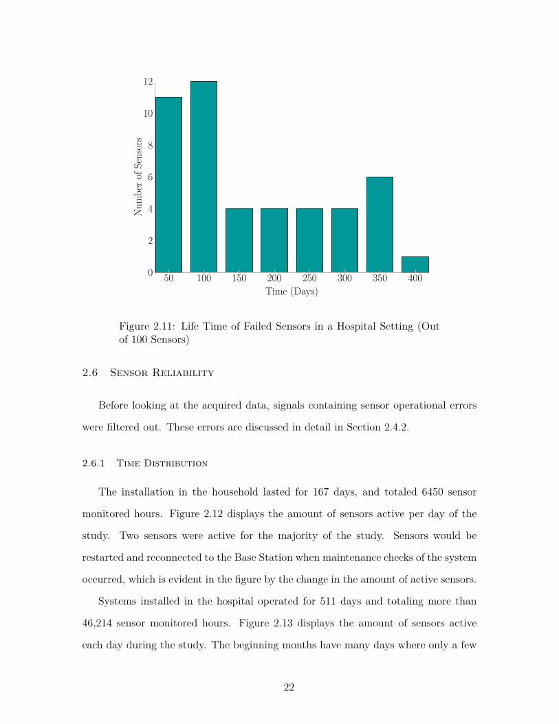
50 100 150 200 250 300 350 400Time (Days)
0
2
4
6
8
10
12
Num
bero
fSen
sors
Figure 2.11: Life Time of Failed Sensors in a Hospital Setting (Outof 100 Sensors)
2.6 Sensor Reliability
Before looking at the acquired data, signals containing sensor operational errors
were filtered out. These errors are discussed in detail in Section 2.4.2.
2.6.1 Time Distribution
The installation in the household lasted for 167 days, and totaled 6450 sensor
monitored hours. Figure 2.12 displays the amount of sensors active per day of the
study. Two sensors were active for the majority of the study. Sensors would be
restarted and reconnected to the Base Station when maintenance checks of the system
occurred, which is evident in the figure by the change in the amount of active sensors.
Systems installed in the hospital operated for 511 days and totaling more than
46,214 sensor monitored hours. Figure 2.13 displays the amount of sensors active
each day during the study. The beginning months have many days where only a few
22
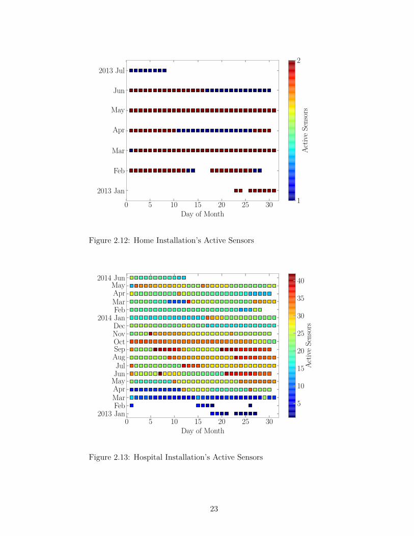
0 5 10 15 20 25 30Day of Month
2013 Jan
Feb
Mar
Apr
May
Jun
2013 Jul
1
2
Activ
eSe
nsor
s
Figure 2.12: Home Installation’s Active Sensors
0 5 10 15 20 25 30Day of Month
2013 JanFebMarAprMayJunJul
AugSepOctNovDec
2014 JanFebMarAprMay
2014 Jun
5
10
15
20
25
30
35
40
Activ
eSe
nsor
s
Figure 2.13: Hospital Installation’s Active Sensors
23
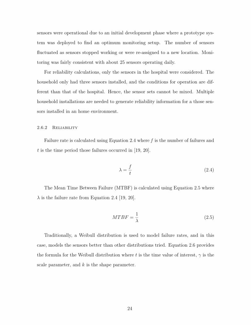
sensors were operational due to an initial development phase where a prototype sys-
tem was deployed to find an optimum monitoring setup. The number of sensors
fluctuated as sensors stopped working or were re-assigned to a new location. Moni-
toring was fairly consistent with about 25 sensors operating daily.
For reliability calculations, only the sensors in the hospital were considered. The
household only had three sensors installed, and the conditions for operation are dif-
ferent than that of the hospital. Hence, the sensor sets cannot be mixed. Multiple
household installations are needed to generate reliability information for a those sen-
sors installed in an home environment.
2.6.2 Reliability
Failure rate is calculated using Equation 2.4 where f is the number of failures and
t is the time period those failures occurred in [19, 20].
λ = f
t(2.4)
The Mean Time Between Failure (MTBF) is calculated using Equation 2.5 where
λ is the failure rate from Equation 2.4 [19, 20].
MTBF = 1λ
(2.5)
Traditionally, a Weibull distribution is used to model failure rates, and in this
case, models the sensors better than other distributions tried. Equation 2.6 provides
the formula for the Weibull distribution where t is the time value of interest, γ is the
scale parameter, and k is the shape parameter.
24

P (t) =
kγ
(tγ
)k−1e−(
tγ
)k
t > 0
0 t ≤ 0(2.6)
The Weibull distribution was fitted using the weibull_min function from SciPy
[21], and a Quantile-Quantile (QQ) plot produced in Figure 2.14 showing a relatively
linear trend. This indicates the distribution is a good fit for the Camp Hill failures.
0 100 200 300 400 500Quantiles
0
100
200
300
400
500
Ord
ered
Valu
es
R2 = 0.9653
Figure 2.14: QQ Plot for a Weibull Distribution Describing the Fail-ure Rate
A truncated normal distribution was tried as in Equation 2.7 where σ is the
standard deviation, µ is the mean, and t is the time value of interest. In this case,
the standard deviation was 110.6 days, and the mean was 170.7 days.
P (t) =
1
σ√
2πe−(t−µ)2/
(2σ2)
t > 0
0 t ≤ 0(2.7)
25
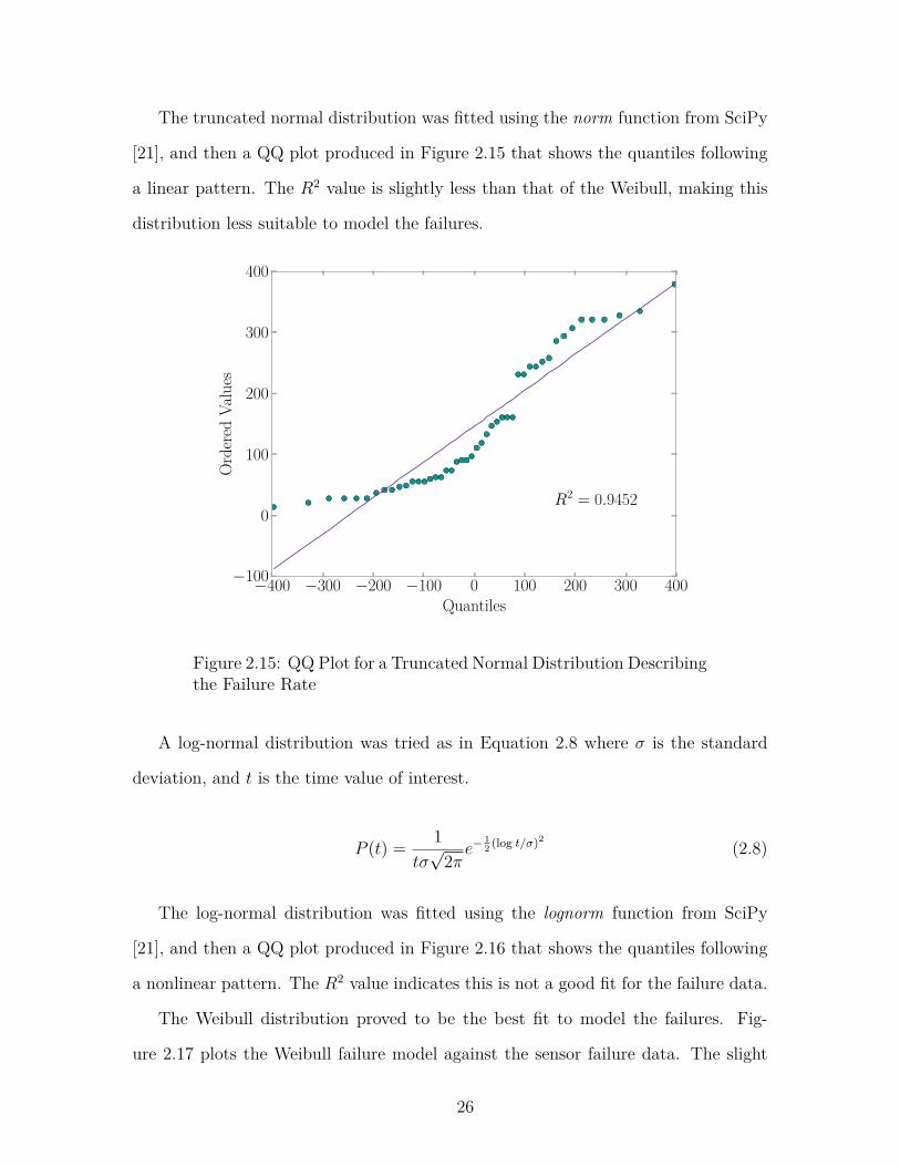
The truncated normal distribution was fitted using the norm function from SciPy
[21], and then a QQ plot produced in Figure 2.15 that shows the quantiles following
a linear pattern. The R2 value is slightly less than that of the Weibull, making this
distribution less suitable to model the failures.
−400 −300 −200 −100 0 100 200 300 400Quantiles
−100
0
100
200
300
400
Ord
ered
Valu
es
R2 = 0.9452
Figure 2.15: QQ Plot for a Truncated Normal Distribution Describingthe Failure Rate
A log-normal distribution was tried as in Equation 2.8 where σ is the standard
deviation, and t is the time value of interest.
P (t) = 1tσ
√2π
e− 12 (log t/σ)2
(2.8)
The log-normal distribution was fitted using the lognorm function from SciPy
[21], and then a QQ plot produced in Figure 2.16 that shows the quantiles following
a nonlinear pattern. The R2 value indicates this is not a good fit for the failure data.
The Weibull distribution proved to be the best fit to model the failures. Fig-
ure 2.17 plots the Weibull failure model against the sensor failure data. The slight
26

0 100 200 300 400 500 600 700 800Quantiles
0
100
200
300
400
500
600
Ord
ered
Valu
es
R2 = 0.8910
Figure 2.16: QQ Plot for a Log-Normal Distribution Describing theFailure Rate
increase in failures around 300 days is not well modeled by the Weibull and con-
tributes to the nonlinear right tail of the Weibull QQ Plot in Figure 2.14. A wear out
failure trend as exhibited in Figure 2.18 was experienced by the sensors. The overall
failure rate is 5.06 × 10⁻³ failureshour , and the MTBF is 197.7 hours.
Expanding this in a probabilistic sense for the likelihood of measuring a fall that
produced a vibration measurable by the sensor, we find that the chance is directly
related to the sensor failure rate as demonstrated in Equation 2.9.
P (Measuring Fall | Measurable Vibration) = P (Sensor Working)
= 1 − P (Sensor Failure)(2.9)
The assumption made here is that a sensor that is operating correctly will have the
capability to correctly identify the impact (identification is being explored in other
research), and the fall occurs in the sensor’s area of influence.
27

0 100 200 300 400 500Time (days)
0.000
0.001
0.002
0.003
0.004
0.005
0.006
Prob
abili
ty
WeibullData
Figure 2.17: Weibull Distribution Failure Model Vs. Sensor Failures
0 100 200 300 400 500Time (days)
0.000
0.002
0.004
0.006
0.008
0.010
0.012
0.014
Failu
reRa
te(fa
ilure
/day
)
Figure 2.18: Sensor Failure Rate Bathtub Curve
28

Using the Weibull distribution fitted above, the likelihood of measuring a fall in
a year using these sensors is 4.9%. This assumes that the algorithms are completely
reliable, and the fall creates measurable accelerations. The MTBF to achieve 99%
likelihood comes out to be 8642.4 hours. This equates to 1.16 × 10⁻⁴ failureshour as an
overall failure rate for a sensor, which is what a manufacturer should aim for when
producing sensors for a fall detection application.
2.7 Description of Collected Data
A total of 21,413 events were captured in the household. Figure 2.19 displays the
distribution of sensor activations during this time period. The beginning of this period
experienced around 260 activations a day, while the end of the period experienced
around 60 events a day. This disparity has to do with system operational issues
towards the end of the study. The laptop started to degrade in performance, and
consequently, the ability to receive and store data. In addition, the residents took a
vacation from May 19 until June 1 as marked on the graph, which, during this time,
no activity was recorded.
Taking all of the activations and compressing them into a week, human activity
trends show a discernible pattern as illustrated in Figure 2.20. Three bands of higher
activity appear around the hours of 8, 12, and 18. These, evidently correspond
with typical daily meal times when there would naturally be a lot of activity in the
household preparing dinner and wrangling children to the dinner table. The sensors
were located in the first floor in the room next to the kitchen and dinning room,
which supports this conclusion. Lighter activity is seen throughout the day time and
almost zero activity is seen during typical sleeping hours (between hours of 22 and
6). The twins regularly took naps around the hours of 10 and 15, which are shown
to be times of lower activity as well. Also, the family attends Sunday church services
around the hours of 9 and 10, which, as the graph displays, have almost zero events.
29
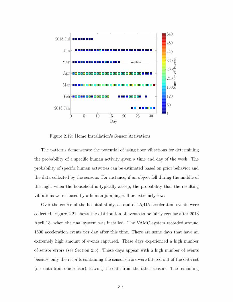
0 5 10 15 20 25 30Day
2013 Jan
Feb
Mar
Apr
May
Jun
2013 Jul
——— Vacation ———
–
1
60
120
180
240
300
360
420
480
540
Num
bero
fEve
nts
Figure 2.19: Home Installation’s Sensor Activations
The patterns demonstrate the potential of using floor vibrations for determining
the probability of a specific human activity given a time and day of the week. The
probability of specific human activities can be estimated based on prior behavior and
the data collected by the sensors. For instance, if an object fell during the middle of
the night when the household is typically asleep, the probability that the resulting
vibrations were caused by a human jumping will be extremely low.
Over the course of the hospital study, a total of 25,415 acceleration events were
collected. Figure 2.21 shows the distribution of events to be fairly regular after 2013
April 13, when the final system was installed. The VAMC system recorded around
1500 acceleration events per day after this time. There are some days that have an
extremely high amount of events captured. These days experienced a high number
of sensor errors (see Section 2.5). These days appear with a high number of events
because only the records containing the sensor errors were filtered out of the data set
(i.e. data from one sensor), leaving the data from the other sensors. The remaining
30
Sun Mon Tue Wed Thu Fri Sat
6
12
18
23
Hou
rofD
ay
80
160
240
320
400
480
560
640
720
Num
bero
fEve
nts
Figure 2.20: Home Installation’s Activity Density
signals are low magnitude signals with a small signal to noise ratio.
A distinct pattern develops when the entire data set is broken down by hour
of the day and overlapped; a pattern which matches what one would expect to see
in a hospital setting (see Figure 2.22). A large amount of events were recorded
during normal business hours on the weekdays and a smaller amount of events are
present on the weekends during all hours. This demonstrates the possibility of using
floor vibrations to study a high traffic area’s activity patterns. These patterns could
further be used for a number of uses. For example, to refine any human fall detection
methodology by introducing probabilities of falls based on the hospital’s routines.
For instance, if a large amount of activity is present around hour 10 normally, then
the probability that a fall would go unnoticed at this time is low, but if a spike of
acceleration occurred at hour 23, then there would be a higher probability of fall
going unnoticed and a monitoring system would raise an alarm.
Different environments produce different activity patterns, which means systems
31

0 5 10 15 20 25 30Day
2013 JanFebMarAprMayJunJul
AugSepOctNovDec
2014 JanFebMarAprMay
2014 Jun
0.0
0.8
1.6
2.4
3.2
4.0
4.8
5.6
6.4
7.2
log(
Num
bero
fEve
nts)
Figure 2.21: Hospital Installation’s Sensor Activations
of sensors will need to learn their own specific environment in order to accurately
identify and even predict actions such as a human falls. This can be vividly seen by
comparing Figure 2.20 and Figure 2.22. For instance, during the nap time hours of
the household, there is little activity because the twins are asleep; however, during
those same hours in the hospital, things are still very much happening as the hospital
never fully sleeps.
2.8 Features of Collected Data
Before looking at the acquired data, signals containing sensor operational errors
were filtered out. The errors are discussed in Section 2.4.
2.8.1 Features Explored
Two typical signal features were used to explore trends in the collected data:
maximum amplitude and signal energy.
32
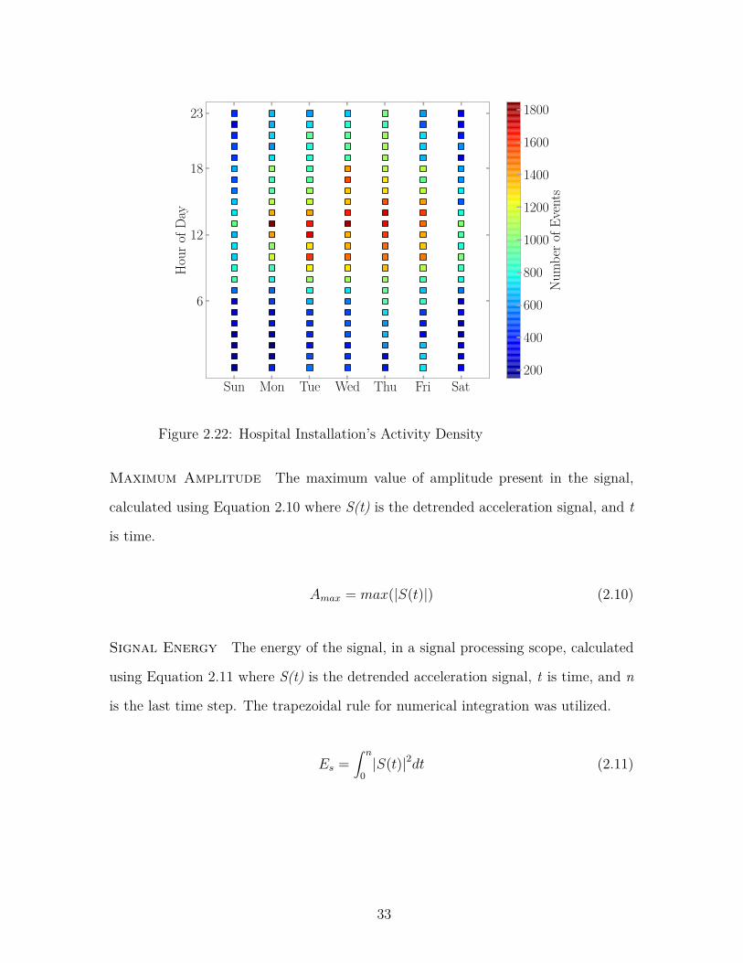
Sun Mon Tue Wed Thu Fri Sat
6
12
18
23
Hou
rofD
ay
200
400
600
800
1000
1200
1400
1600
1800
Num
bero
fEve
nts
Figure 2.22: Hospital Installation’s Activity Density
Maximum Amplitude The maximum value of amplitude present in the signal,
calculated using Equation 2.10 where S(t) is the detrended acceleration signal, and t
is time.
Amax = max(|S(t)|) (2.10)
Signal Energy The energy of the signal, in a signal processing scope, calculated
using Equation 2.11 where S(t) is the detrended acceleration signal, t is time, and n
is the last time step. The trapezoidal rule for numerical integration was utilized.
Es =∫ n
0|S(t)|2dt (2.11)
33
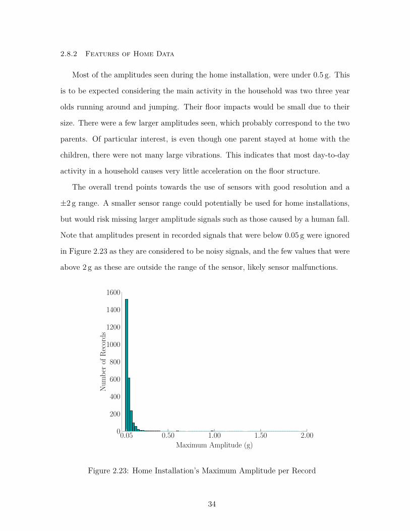
2.8.2 Features of Home Data
Most of the amplitudes seen during the home installation, were under 0.5 g. This
is to be expected considering the main activity in the household was two three year
olds running around and jumping. Their floor impacts would be small due to their
size. There were a few larger amplitudes seen, which probably correspond to the two
parents. Of particular interest, is even though one parent stayed at home with the
children, there were not many large vibrations. This indicates that most day-to-day
activity in a household causes very little acceleration on the floor structure.
The overall trend points towards the use of sensors with good resolution and a
±2 g range. A smaller sensor range could potentially be used for home installations,
but would risk missing larger amplitude signals such as those caused by a human fall.
Note that amplitudes present in recorded signals that were below 0.05 g were ignored
in Figure 2.23 as they are considered to be noisy signals, and the few values that were
above 2 g as these are outside the range of the sensor, likely sensor malfunctions.
0.05 0.50 1.00 1.50 2.00Maximum Amplitude (g)
0
200
400
600
800
1000
1200
1400
1600
Num
bero
fRec
ords
Figure 2.23: Home Installation’s Maximum Amplitude per Record
34

The signal energy for each record was calculated to give a measure of how much
activity a sensor caught in each record. The majority of signals, a lot of which are
noise, had very low signal energy, while those with activity tended to have relatively
higher values. Figure 2.24 displays this trend. Note that outlier values, those above
0.0005 g2 s are not displayed. There were very few of these signals and corresponded
with records containing cyclic patterns, which are most likely caused by a machine,
and thus were not included here.
The two signal features were plotted against each other in Figure 2.25 to see
if there was a correlation between the two. Groupings would allow machine learn-
ing techniques coupled with probabilistic methods to generate the likelihood a fall
occurred and other activities occurred. Research is ongoing in this regard.
0E+00 1E-04 2E-04 3E-04 4E-04 5E-04Signal Energy (g2 · s)
0
1000
2000
3000
4000
5000
6000
7000
8000
Num
bero
fRec
ords
Figure 2.24: Home Installation’s Signal Energy Per Record
35

0E+00 1E-04 2E-04 3E-04 4E-04 5E-04Signal Energy (g2 · s)
0.0
0.5
1.0
1.5
2.0
Max
imum
Am
plitu
de(g
)
Figure 2.25: Home Installation’s Maximum Amplitude Vs. SignalEnergy
2.8.3 Features of Hospital Data
Amplitudes present in records capture from the hospital tended to be small in
magnitude (<0.5 g), with a bunch of outlying records having around 2 g. The lower
amplitudes were expected due to the nature of the stiffness of reinforced concrete
flooring, and the tight regulations on hospitals to limit vibrations [18]. The larger
amplitudes were caused by a mixture of impacts close to the location of the sensor,
and patients picking up the sensors, perhaps thinking they USB power sources were
chargers for their phones (see Section 2.4).
The overall trend points towards the use of sensors with good resolution and a
±2 g range. Note that amplitudes present in recorded signals that were below 0.05 g
were ignored in Figure 2.26 as they are considered to be noisy signals, and the few
values that were above 2 g as these are outside the range of the sensor, likely sensor
malfunctions.
36

0.05 0.50 1.00 1.50 2.00Maximum Amplitude (g)
0
500
1000
1500
2000
Num
bero
fRec
ords
Figure 2.26: Hospital Installation’s Maximum Amplitude Per Record
0 5 10 15 20Signal Energy (g2 · s)
0
200
400
600
800
1000
1200
1400
1600
1800
Num
bero
fRec
ords
Figure 2.27: Hospital Installation’s Signal Energy Per Record
37

0 5 10 15 20Signal Energy (g2 · s)
0.0
0.5
1.0
1.5
2.0
Max
imum
Am
plitu
de(g
)
Figure 2.28: Hospital Installation’s Maximum Amplitude Vs. SignalEnergy
Signal energy present in the hospital installation are grouped mostly between 8 g2 s
and 15 g2 s, indicating accelerations observed have a similar amount of activity. Note
that values below 0.1 g2 s were removed as records with those values are considered
to be noise.
The two signal features were plotted against each other in Figure 2.28 to see
if there was a correlation between the two. Groupings would allow machine learn-
ing techniques coupled with probabilistic methods to generate the likelihood a fall
occurred and other activities occurred. Research is ongoing in this regard.
2.9 Hospital Reported Human Falls
For the length of the study, 50 fall events were reported by the hospital staff (see
Table A.1). The estimated time of each fall was given to researchers to be used to
correlate with collected acceleration records. Challenges arose because the of human
38

error when reporting the time and because the times reported are the time the patient
was found and not necessarily the actual time of the event. Hospital patients are
monitored on a regular schedule along with constant patrols and emergency pendants
the patients can press to call for nurse assistance which aids to reduce reported time
error. Additionally, the base station computers’ time may also be off since they were
not connected to the Internet where the computers could get constant time updates
based on an atomic clock. Researchers thus look at a ±1 hour window based on
the reported time to account for these potentials for error. Of those 50 reported,
four occurred before the room had a system installed and one did not have enough
information to identify the system that would have recorded the event. Researchers
found records correlating with 16 reports of the remaining 45 records.
0 5 10 15 20 25 30 35Number of Events
Reco
rded
Not
Reco
rded
ActiveInactive
Figure 2.29: Comparison of Hospital Reported Falls to System Cap-tured Falls
Sometimes during operations, the sensors would fail (see Section 2.5) and become
inactive leading to missed fall events, and other times, the event was missed entirely
39

even though the sensors were active. The latter may be due to the larger error in time
reporting than accounted for (discussed above) or the impact from the fall resulting
in a slight vibration that the sensors could not detect. Figure 2.29 demonstrates these
challenges. Sensors were active during 26 reported events, but only capturing 16 of
those 26. This equates to a ∼62% successful capture rate.
2.10 Real Falls vs Recorded Falls
2.10.1 Recorded Falls
Table 2.2 compares the reported to the collected events and rates the researcher’s
confidence (0 being no confidence, 5 being very confident) that the fall event was
captured based on the collection time and the actual signal. Figure 2.30 visualizes
the dates demonstrating human error in the reporting process.
Sun Mon Tue Wed Thu Fri Sat0
6
12
18
23
Hou
rofD
ay
Reported Falls Recorded Data
Figure 2.30: Visualization of Reported Falls Vs. Captured Falls
40
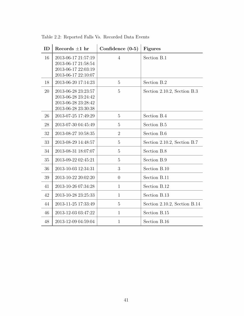
Table 2.2: Reported Falls Vs. Recorded Data Events
ID Records ±1 hr Confidence (0-5) Figures
16 2013-06-17 21:57:192013-06-17 21:58:542013-06-17 22:03:192013-06-17 22:10:07
4 Section B.1
18 2013-06-20 17:14:23 5 Section B.2
20 2013-06-28 23:23:572013-06-28 23:24:422013-06-28 23:28:422013-06-28 23:30:38
5 Section 2.10.2, Section B.3
26 2013-07-25 17:49:29 5 Section B.4
28 2013-07-30 04:45:49 5 Section B.5
32 2013-08-27 10:58:35 2 Section B.6
33 2013-08-29 14:48:57 5 Section 2.10.2, Section B.7
34 2013-08-31 18:07:07 5 Section B.8
35 2013-09-22 02:45:21 5 Section B.9
36 2013-10-03 12:34:31 3 Section B.10
39 2013-10-22 20:02:20 0 Section B.11
41 2013-10-26 07:34:28 1 Section B.12
42 2013-10-28 23:25:33 1 Section B.13
44 2013-11-25 17:33:49 5 Section 2.10.2, Section B.14
46 2013-12-03 03:47:22 1 Section B.15
48 2013-12-09 04:59:04 1 Section B.16
41

2.10.2 Sample Records
A few collected records stand out to the research team and are presented in this
section. The remainder of collected fall events are presented in Appendix B.
Fall Reported on 2013-06-28 23:20 (ID 20)
According the description of this event, the patient was found kneeling next to
the bed after attempting to get up and walk around. This is an interesting sequence
of events with several captured records in close proximity to the reported time the
fall occurred. The first signal shown in Figure 2.31 looks like a jostling movement
which is interpreted to be the patient shifting towards the edge of the bed.
The patient attempted to get up to stretch his legs after shifting to the edge of
the bed. Instead, he fell to the floor to land (we assume) on his knees. Figure 2.32
shows a signal that looks like one knee hit with the majority of the person’s weight,
and another knee followed more gently after the initial impact of the first.
0 2 4 6 8 10 12Time (s)
−0.08
−0.06
−0.04
−0.02
0.00
0.02
0.04
0.06
0.08
0.10
Acce
lerat
ion
(g)
Figure 2.31: Fall Event 2013-06-28 23:23:57
42

0 2 4 6 8 10 12Time (s)
−0.10
−0.05
0.00
0.05
0.10
0.15
0.20
0.25
0.30
Acce
lerat
ion
(g)
Figure 2.32: Fall Event 2013-06-28 23:24:42
0 2 4 6 8 10 12Time (s)
−0.10
−0.05
0.00
0.05
0.10
0.15
Acce
lerat
ion
(g)
Figure 2.33: Fall Event 2013-06-28 23:28:42
43

Within a few minutes, the patient may have attempted to get back up onto the bed
but was unsuccessful leading to another impact on the floor as he dropped back down.
Figure 2.33 shows a downward impact with a slightly higher downward amplitude
(∼0.08 g) than the first time the patient fell in Figure 2.32 which suggests more force
was applied to the floor, like the full weight of the patient.
Fall Reported on 2013-08-29 14:40 (ID 33)
A nurse was helping the patient, in this instance, to the bedside commode. They
did not make all the way and the patient lost balance falling to the floor. The fall
was broken by the nurse who eased the patient onto the floor lessening the impact.
What is of interest for this event the mode which involves one person ‘damping’ the
impact and that two sensors, one inside (Figure 2.34) and one outside of the room
(Figure 2.35), showed similar acceleration patterns.
0 2 4 6 8 10 12Time (s)
−0.08
−0.06
−0.04
−0.02
0.00
0.02
0.04
0.06
Acce
lerat
ion
(g)
Figure 2.34: Fall Event 2013-08-29 14:48:57 - Sensor Inside Room
44

0 2 4 6 8 10 12Time (s)
−0.04
−0.02
0.00
0.02
0.04
0.06
Acce
lerat
ion
(g)
Figure 2.35: Fall Event 2013-08-29 14:48:57 - Sensor Outside Room
Notice how each sensor picked up three consecutive hits at approximately the
same time within the record, with the sensor that is in the room of the event expe-
riencing slightly higher accelerations than that of the sensor outside the room. The
response demonstrates the low reliability of determining a fall directly from ampli-
tude alone but points towards the possibility of using records from multiple sensors to
develop a probability that the event occurred. A research topic the team is currently
investigating.
Fall Reported on 2013-11-25 17:45 (ID 44)
The patient in this scenario bent over to pick up some trash off the floor before
losing his balance and falling down. Assuming the he bent at the waist and tumbled
in the direction of his bending, the natural defensive response would be to attempt to
break the fall using ones arms before the rest of the body lands. Figure 2.36’s signal
displays that pattern with the first peak being smaller than the second.
45
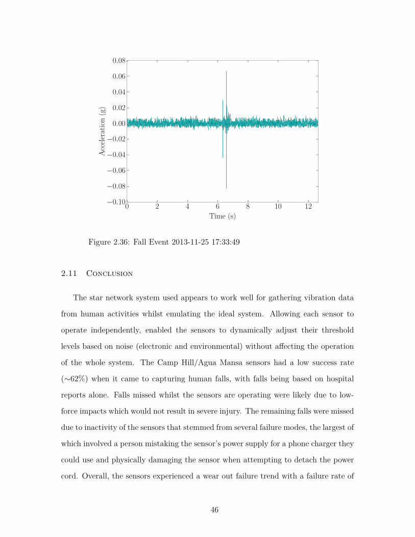
0 2 4 6 8 10 12Time (s)
−0.10
−0.08
−0.06
−0.04
−0.02
0.00
0.02
0.04
0.06
0.08
Acce
lerat
ion
(g)
Figure 2.36: Fall Event 2013-11-25 17:33:49
2.11 Conclusion
The star network system used appears to work well for gathering vibration data
from human activities whilst emulating the ideal system. Allowing each sensor to
operate independently, enabled the sensors to dynamically adjust their threshold
levels based on noise (electronic and environmental) without affecting the operation
of the whole system. The Camp Hill/Agua Mansa sensors had a low success rate
(∼62%) when it came to capturing human falls, with falls being based on hospital
reports alone. Falls missed whilst the sensors are operating were likely due to low-
force impacts which would not result in severe injury. The remaining falls were missed
due to inactivity of the sensors that stemmed from several failure modes, the largest of
which involved a person mistaking the sensor’s power supply for a phone charger they
could use and physically damaging the sensor when attempting to detach the power
cord. Overall, the sensors experienced a wear out failure trend with a failure rate of
46

5.06×10⁻³ failureshour and a MTBF is 197.7 hours. The likelihood of this sensor to capture
a fall in its current state is 4.9%. In order to have a 99% likelihood of capturing a
fall, a sensor’s MTBF should be 8642.4 hours based on a Weibull distribution.
Other aspects of the sensor emerged, including recommendations of buffer size,
sampling rate, and sensitivity for wireless accelerometers for human activity monitor-
ing, in particular human fall detection. These factors are chosen as they are general
enough that every wireless sensor working with human-induced vibrations would uti-
lize them. Factors such as operational temperature range are not explored as they
are specific to the environment one would install the sensor and should be made on
a case-by-case basis.
The current recommendation for a buffer size (e.g. amount of time needed to fully
capture a vibrations from a fall) is 3 s [6]. This suggestion holds up when looking
at the 16 fall events captured by the system for purely capturing the vibrations of
the fall. One may wish to increase the buffer size for handling various fall detection
algorithms, however. Sampling rate of the sensors was 316 Hz, working well in both
the home and hospital installations. This rate is not a typical hardware enabled
rate for wireless accelerometers, so it is suggested to use the more common rate of
400 Hz which will also give signals some more definition. Sensitivity of the installed
sensors, the remaining aspect, was 0.25 mg resolution and a range of ±2 g. The range
proved more than enough in the falls the systems experienced, with no cutting off
of the signals. However, the resolution was not enough in several of the cases, and
several events were missed potentially due to the fall having low-force which a higher
resolution sensor could have registered. A suggested resolution of 1 µg is put forth to
have better definition in the signal, particularly for falls resulting in low amplitude
vibrations.
Preliminary looks at human activity monitoring through structural vibrations
shows promise. Schedules of the people in hospital and the home installations match
47

closely to what the system saw in vibrations as seen in the heat maps presented.
Further research into predictive activity models would open up many avenues for
development of privacy-respecting technology towards more intelligent infrastructure.
48

Chapter 3
Data Management For Structural Vibration
Monitoring of Human Activity
3.1 Introduction
A large amount of data is produced from a large scale installation of the vibra-
tion monitoring system described in Chapter 2. Thus, a way to keep track of all the
data in a meaningful way so that researchers can focus more on analysis and not on
organization of all the data is needed. This is called data curation and is “the ac-
tive and ongoing management of data through its life cycle of interest and usefulness
to scholarship, science, and education” [22]. The field itself “includes authentica-
tion, archiving, management, preservation, retrieval, and representation” [22]. As a
first step towards curation of the data generated by this work, a data management
plan was devised and implemented. The devised strategy focused on flexibility for
scalability through a relational database architecture, as well as leveraging secure
websites interfaces for tracking other information related to the project. Addition-
ally, a Python package was created to streamline access to the database allowing for
researchers to gather information with ease.
3.2 Management Plan
All data gathered and generated is housed on servers of the Structural Dynamics
and Intelligent Infrastructure Laboratory (SDII) at the University of South Carolina
(USC). The following sections describe the data being collected and its management.
49
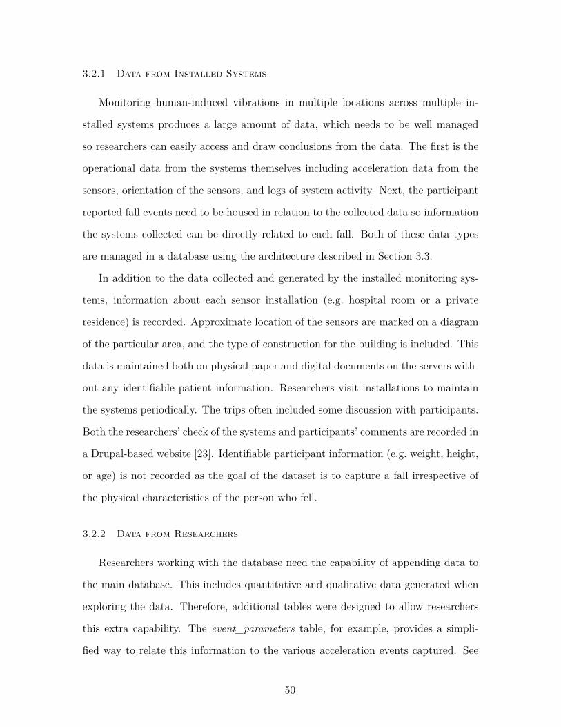
3.2.1 Data from Installed Systems
Monitoring human-induced vibrations in multiple locations across multiple in-
stalled systems produces a large amount of data, which needs to be well managed
so researchers can easily access and draw conclusions from the data. The first is the
operational data from the systems themselves including acceleration data from the
sensors, orientation of the sensors, and logs of system activity. Next, the participant
reported fall events need to be housed in relation to the collected data so information
the systems collected can be directly related to each fall. Both of these data types
are managed in a database using the architecture described in Section 3.3.
In addition to the data collected and generated by the installed monitoring sys-
tems, information about each sensor installation (e.g. hospital room or a private
residence) is recorded. Approximate location of the sensors are marked on a diagram
of the particular area, and the type of construction for the building is included. This
data is maintained both on physical paper and digital documents on the servers with-
out any identifiable patient information. Researchers visit installations to maintain
the systems periodically. The trips often included some discussion with participants.
Both the researchers’ check of the systems and participants’ comments are recorded in
a Drupal-based website [23]. Identifiable participant information (e.g. weight, height,
or age) is not recorded as the goal of the dataset is to capture a fall irrespective of
the physical characteristics of the person who fell.
3.2.2 Data from Researchers
Researchers working with the database need the capability of appending data to
the main database. This includes quantitative and qualitative data generated when
exploring the data. Therefore, additional tables were designed to allow researchers
this extra capability. The event_parameters table, for example, provides a simpli-
fied way to relate this information to the various acceleration events captured. See
50

Section 3.3 for more discussion and description about this and other tables.
3.2.3 Data Access
Access to the data is controlled through log in credentials for each user. This
allows for the control of what each user can do with the database so as to prevent
accidental changes. In addition, each installed system maintains a local database that
mirrors the one housed with SDII as an additional precaution. A Python package
(ssh_database_utilities) standardizes data access to the database which additionally
aids in reducing unwanted accidental changes to stored information. The package
documentation is available in Appendix M. For those given more direct access to the
database, sample queries are provided in Appendix C.
3.3 Database Architecture
A relational database was chosen to store and access the experimental data, using
MySQL as the backend [24]. The enhanced entity relationship diagram is presented
in Figure 3.1. This database structure is used at the site where data is collected in
the base stations and in the main database. The following paragraphs describe the
tables in more detail, and are organized in alphabetical order for easy reference. The
term ‘event’ means the monitoring system was triggered to record accelerations from
its sensors thus indicating one or more recorded signals, and the term ‘hit’ means an
impact present in a signal.
51
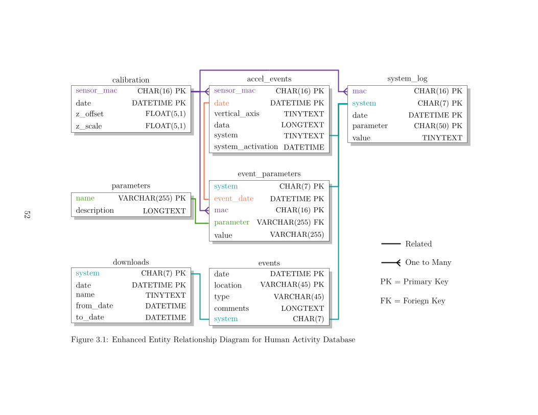
sensor_mac CHAR(16) PKdate DATETIME PKz_offset FLOAT(5,1)z_scale FLOAT(5,1)
calibrationsensor_mac CHAR(16) PKdate DATETIME PKvertical_axis TINYTEXTdata LONGTEXTsystem TINYTEXTsystem_activation DATETIME
accel_eventsmac CHAR(16) PKsystem CHAR(7) PKdate DATETIME PKparameter CHAR(50) PKvalue TINYTEXT
system_log
name VARCHAR(255) PKdescription LONGTEXT
parameters system CHAR(7) PKevent_date DATETIME PKmac CHAR(16) PKparameter VARCHAR(255) FK
value VARCHAR(255)
event_parameters
system CHAR(7) PKdate DATETIME PKname TINYTEXTfrom_date DATETIMEto_date DATETIME
downloadsdate DATETIME PKlocation VARCHAR(45) PKtype VARCHAR(45)comments LONGTEXTsystem CHAR(7)
events
Related
One to Many
PK = Primary Key
FK = Foriegn Key
Figure 3.1: Enhanced Entity Relationship Diagram for Human Activity Database
52

accel_events Here, all the data collected from the sensors is stored including
information about the orientation of the sensor and the system the sensor belongs
to. Each table row has a system and system_activation for referencing items stored
in the system_log table. Knowing when the system was activated allows one to grab
information from the log pertaining to a specific operational period of the system.
The acceleration data captured is first converted into units of gravity through the
calibration table, and then, is stored as a space delimited string in the field data.
calibration The Agua Mansa sensors report data to the base station in pts/g,
where the data needs to be converted into units of acceleration. This table stores
the calibration information with the base station using the latest dated calibration
values for unit conversion. Sensor Media Access Control Addresses (MAC Addresses)
must be available in the calibration table before data is recorded into the accel_event
table. Base station programs enforce this policy. For more information on calibration
and conversion formulas see Section 2.3.1.
downloads This table is used to track when data from a system for a specific
time period has been transfered from the base station to the SDII servers. When
downloading data, the user enters his name or, in the case of the web service, the name
webservice is entered. Subsequent downloads of data from a base station reference
the table to reduce the amount of data to transfer in each download, and thus the
amount of time it takes for the download process. This is used in the base station for
use with the Data Mobile Ubiquitous LAN Extension (MULE), and the main server
for use with the web service (see Section 2.3.1 for more details).
events All reported human-induced vibration events are recorded here with in-
formation on the system that saw the event, the date and time the event occurred,
comments from the reporter, and the location of installation. No patient information
53

(e.g. name, weight) is stored to protect privacy. The field type intentionally is flexible
if other significant human activity besides a human fall is reported as this can be of
interest for refining fall detection algorithms or research into other activity.
event_parameters Acceleration events have various parameters, or metrics, that
can be used to describe them. Calculated metrics from the parameters table are
stored in this table for signals present in accel_events. This includes parameters
like maximum amplitude and signal category. Access the parameters database table
for a current list of available metrics created by this research and their descriptions.
Table 3.1 provides the parameters available at the time of this writing.
parameters The parameter table defines parameters and removes the chance that
a it can be misspelled. Other tables reference this one via foreign keys to ensure
integrity. Table 3.1 describes the parameters, available as of 2016 February 1, in
alphabetical order by their database names.
Table 3.1: Acceleration Parameters
Name DB Name Description
Amplitude Hits amphit Amplitude within the record (g);There is one number per hit
Maximum Amplitude ampmax Max of the absolute value of thesignal (g); See Section 4.2.2
Manual Category category-manual Category of signal manually clas-sified: (0) not sure what category,(1) noise, (2) some activity but in-distinct peaks or shape, (3) dis-tinct peaks and shape, (4) sensorerror; Used for training an SVM
continued on next page. . .
54

Name DB Name Description
SVM Category category-svm Category of signal created by theSVM: (0) not sure what category,(1) noise, (2) some activity but in-distinct peaks or shape, (3) dis-tinct peaks and shape; See Chap-ter 4
Dispersion Ratio dr The ratio of desired signal to envi-ronmental noise; See Section 4.2.5
Error errornorm Normalized error of the exponen-tial curve
Location location Location of the event; For exam-ple, a specific room in a house
Max AmplitudeDifference mad The max change between descend-
ing sorted, absolute values of thesignal (g); NaN are ignored; SeeSection 4.2.3
Accepted Hits naccept Number of hits accepted duringanalysis
NaN Density nandensity The density of NaN values in therecord; See Section 4.2.1
Number Rejected nreject Number of potential hits rejectedduring analysis
Rate of Dispersion rod How much dispersion is presentwithin a signal; See Section 4.2.4
Signal Energy senergy Energy present in a signal process-ing sense (g2 s); See Section 2.8.1
Hit Time thit Time of impacts within the record(in seconds since the beginning ofthe record); There is one numberper hit
Natural Freq. andDamping wnzetahit Estimation of ωnζ for each hit
within the record
55

system_log The system log tracks activity of the system, including errors and
installation dates, during a system’s operation. This is for both the base station and
the sensors themselves. Base stations (i.e. the laptops) store a blank string, 0, or
their MAC Addresses for the field mac. Sensors store in the log using their own MAC
Addresses so parameters such as reliability or actual sampling rate can be determined
(see Chapter 2). The table does not reference another table by foreign key unlike that
of the parameter and event_parameter table relationship. This allows for maximum
flexibility when programming the system so that new log info can be added at will.
Thus, parameter names in this table tend to be more verbose and self-descriptive for
clarity. Table 3.2 describes the parameters in the system logs, as of 2016 February 1,
in alphabetical order of their database names.
Table 3.2: Parameters in the System Log Table
DB Name Description
data_received Number of data points received fromthe sensor in the time span er-ror_log_length
error_log_length Length of time between system logsaves (s); Saved when system starts
installed Indicates system installed, referencethe date of the log for when the installoccurred
lost_sync Number of times the base station lostsynchronization with a sensor in thetime span error_log_length
malformed_data Number of bad data packets receivedby the base station for the sensor inthe time span error_log_length
continued on next page. . .
56
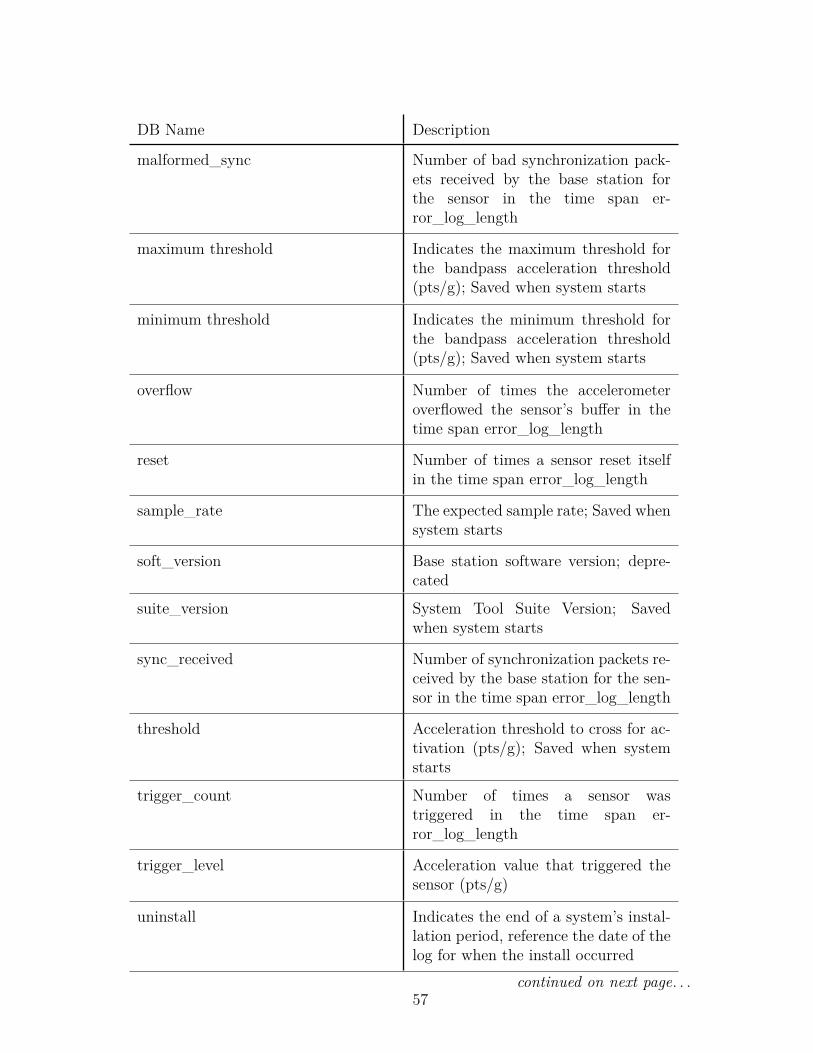
DB Name Description
malformed_sync Number of bad synchronization pack-ets received by the base station forthe sensor in the time span er-ror_log_length
maximum threshold Indicates the maximum threshold forthe bandpass acceleration threshold(pts/g); Saved when system starts
minimum threshold Indicates the minimum threshold forthe bandpass acceleration threshold(pts/g); Saved when system starts
overflow Number of times the accelerometeroverflowed the sensor’s buffer in thetime span error_log_length
reset Number of times a sensor reset itselfin the time span error_log_length
sample_rate The expected sample rate; Saved whensystem starts
soft_version Base station software version; depre-cated
suite_version System Tool Suite Version; Savedwhen system starts
sync_received Number of synchronization packets re-ceived by the base station for the sen-sor in the time span error_log_length
threshold Acceleration threshold to cross for ac-tivation (pts/g); Saved when systemstarts
trigger_count Number of times a sensor wastriggered in the time span er-ror_log_length
trigger_level Acceleration value that triggered thesensor (pts/g)
uninstall Indicates the end of a system’s instal-lation period, reference the date of thelog for when the install occurred
continued on next page. . .57

DB Name Description
webservice-accel_events-duplicates Number of duplicate accelerationevent records the web service tried toupload
webservice-accel_events-failure Indicates the web service failed to up-load acceleration events
webservice-accel_events-sent Number of acceleration event recordsthe web service sent
webservice-accel_events-timeout Number of timeouts the web servicehad when trying to send accelerationevent data
webservice-calibration-duplicates Number of duplicate calibrationrecords the web service tried toupload
webservice-calibration-failure Indicates the web service failed to up-load calibrations
webservice-calibration-sent Number of calibration records the webservice sent
webservice-calibration-timeout Number of timeouts the web servicehad when trying to send calibrationdata
webservice-downloads-duplicates Number of duplicate download recordsthe web service tried to upload
webservice-downloads-failure Indicates the web service failed to up-load downloads
webservice-downloads-sent Number of download records the webservice sent
webservice-downloads-timeout Number of timeouts the web servicehad when trying to send downloadsdata
webservice-system_log-duplicates Number of duplicate system logrecords the web service tried to upload
webservice-system_log-failure Indicates the web service failed to up-load system logs
continued on next page. . .
58

DB Name Description
webservice-system_log-sent Number of system log records the webservice sent
webservice-system_log-timeout Number of timeouts the web servicehad when trying to send system logsdata
3.4 Conclusion
The data management plan outlined in this chapter, has worked well over the
many years of the human activity through structural vibrations study and provides
a foundation for future data curation. Researchers have the infrastructure to handle
and analyze the multitude of acceleration records collected, as well as tools for easy
access to data while mitigating the possibility of accidental changes in the data.
Identifiable participant information is not recorded, providing privacy and promoting
research towards user-independent fall detection. The flexibility and scalability of
this plan will provide valuable research infrastructure for years to come.
59

Chapter 4
Acceleration Event Filtering
4.1 Introduction
The Structural Dynamics and Intelligent Infrastructure Laboratory (SDII) at the
University of South Carolina (USC) houses 536,686 acceleration records constitut-
ing 220,597 distinct events as of 2016 February 1, with more being gathered daily.
These records are collected as a joint effort between SDII, Palmetto Health Hospi-
tal (PH), and the William Jennings Bryan Dorn Veteran’s Administration Medical
Center (VAMC) to capture human-induced vibrations from a variety of environments
including hospitals, nursing homes, and personal residences. The aim of the effort
is to investigate human activity as it relates to changes in medical conditions using
vibrations of the structural as the sole point of reference. Needless to say, vibration
based human monitoring systems produce a considerable amount of data which create
the challenge of identifying relevant records to study or consider for further action.
Data is often collected using wireless accelerometers, and with that comes addi-
tional challenges as wireless communication is not always reliable leading to dropped
packets on the network meaning parts of the signals can be missing. Another chal-
lenge comes from the reliability of the sensors which can degrade over time under con-
tinuous operation and transmit error-ridden data (details discussed in Section 2.5).
Hence, signal metrics were developed and employed through a Support Vector Ma-
chine (SVM) to sort the database of signals into categories, greatly reducing the
amount of human labor required to get to the ‘meat’ of the database.
60

4.2 Acceleration Signal Metrics
In addition to typical characteristics of the signal such as amplitude, several met-
rics were developed for describing the records which would then be used by the SVM
to learn what the researcher judged to be a good signal. The metrics NaN Density
and MADr served to indicate the cleanliness of the signal with respect to potential
sensor errors. The remainder of the metrics were used to describe the level of activity
present. A signal with little activity is often unwanted for processing techniques as
the data does not contain much information beyond what the sensor quantization
levels are, hence, a way to filter out weak signals is necessary to help the analyst find
quality signals quickly or for computer code to select signals autonomously. All these
metrics are calculated after the mean of the signal has been subtracted to each point.
4.2.1 NaN Density
Sometimes with wireless accelerometers, there will be lost data because of dropped
communication packets. Synchronization techniques allow for the host to determine
missing packets and how many data points are lost. The lost data points are replaced
with a place-holder such as the symbol NaN which stands for ‘Not a Number.’ The
more missing packets, the less reliable the data is. In an effort to easily identify the
signals with a multitude of missing data points, the metric NaN Density was created.
It simply counts the number of NaN place-holders and ratios it to the number of
points in the entirety of the record. Equation 4.1 displays the calculation where nnan
is the number of points in the signal that indicate missing data, and ns are the total
number of points in the acceleration signal.
ρnan = nnan
ns
(4.1)
61

As can be seen from above, the lower the amount of lost data packets, the lower
the ratio with 0.0 being a record without any missing packets. See Figure 2.3 for a
signal missing data.
4.2.2 Maximum Amplitude
This is a simple metric that determines the maximum absolute value of the signal
as shown in Equation 4.2 where max() is the maximum value function, S(t) is the
detrended acceleration signal, and t is time.
Amax = max (|S(t)|) (4.2)
4.2.3 Maximum Amplitude Difference Ratio (MADr)
This metric determines the maximum change between values of consecutive points
within the acceleration signal. Sometimes, the accelerometer may malfunction and
produce a fictitious high-value amplitude point or a ‘spike’ (see Figure 2.9). Accel-
eration records from real events would follow a shape similar to an impulse response
function. Thus the Maximum Amplitude Difference (MAD) gives a sense of discon-
tinuities in the signal that are not due to a physical action.
First, the descending-sorted absolute value of the acceleration signal S(t) is cal-
culated using Equation 4.3 where desc() is the descending order sorting function.
D = desc (|S(t)|) (4.3)
Next, Equation 4.4 expresses the calculation of Maximum Amplitude Difference
(MAD) where max() is the maximum value function, Di is calculated in Equation 4.3,
and i is the index within D.
62

MAD = max (Di − Di−1) (4.4)
Finally, take this value in ratio with the maximum amplitude like in Equation 4.5
where MAD is the maximum amplitude difference calculated using Equation 4.4, and
Amax is the maximum amplitude in the signal calculated using Equation 4.2.
MADr = MADAmax
(4.5)
The closer the MADr is to 1.0, the sharper the change between consecutive points
is. Typically, a ratio greater than 0.95 indicates a ‘spike’ in the data.
4.2.4 Rate of Dispersion (RoD)
The maximum change of the dispersion present of the signal can serve as an indi-
cation of how spread the acceleration signal is. First, a vector of standard deviations
σ‡ is computed like in Equation 4.6 where σ() is the standard deviation, Si is the i-th
point of the acceleration signal, and j is an integer that adjusts the window location
where the standard deviation is calculated.
{σ‡} =
σ (Si:i+nw)
σ (Si+∆:i+∆+nw)...
σ (Si+j∆:i+j∆+nw)
(4.6)
The window shift ∆ is calculated using Equation 4.7
∆ = nw − no (4.7)
63

where nw is the number of points per window, and no is the number of overlapping
points per window. RoD is calculated using Equation 4.8 where τ is an integer.
RoD = max(∣∣∣σ‡
i+τ − σ‡i
∣∣∣) (4.8)
An example of what the metric calculation process looks like is presented in the
following with two signal examples to demonstrate how the rate changes: free vibra-
tion (Signal A) in Figure 4.1a, and a harmonic vibration (Signal B) in Figure 4.1b.
For the example, the value of nw is 250, no is 249, and τ is 100. Notice how the Rate
of Dispersion (RoD) in Signal A is several magnitudes higher than that of the more
regular vibration of Signal B which has more regular dispersion of data points (Fig-
ure 4.1e and Figure 4.1f). This demonstrates how changes in accelerations present in
a signal can be indicated using RoD.
4.2.5 Dispersion Ratio (DR)
This metric attempts to characterize the strength of the desired signal compared
against other sources of vibration considered ‘environmental noise.’ In the case of
human activity, environmental noise would be something like a washing machine
running, and a desired signal would be free vibration wave forms resulting from
impacts. One challenge associated with evaluating the amount of environmental noise
is that one needs to have a record that is only noise. The amount of environmental
noise is different for each sensor installation, and it might even change as a function of
time. It is not practical to manually study noisy signals for each case and determine
the level of environmental noise. An alternative method is presented here where the
vector of standard deviations is calculated using Equation 4.6 and values are extracted
to create a ratio between the signal of interest and the environmental noise in the
same record. The dispersion ratio is defined in Equation 4.9 where max() is
64

0 2 4 6 8 10 12Time (s)
−0.8−0.6−0.4−0.2
0.00.20.40.6
Acce
lerat
ion
(g)
(a) Signal A
0 2 4 6 8 10 12Time (s)
−0.6
−0.4
−0.2
0.0
0.2
0.4
0.6
Acce
lerat
ion
(g)
(b) Signal B
0 2 4 6 8 10 12Time (s)
0.000.050.100.150.200.250.300.350.40
σ‡
(g)
(c) σ‡ for Signal A
0 2 4 6 8 10 12Time (s)
0.000.050.100.150.200.250.300.350.40
σ‡
(g)
(d) σ‡ for Signal B
0 2 4 6 8 10 12Time (s)
0.00
0.02
0.04
0.06
0.08
0.10
0.12
|σ‡ i+
τ−
σ‡ i|(
g)
RoD = 0.11g
(e) RoD for Signal A
0 2 4 6 8 10 12Time (s)
0.00
0.02
0.04
0.06
0.08
0.10
0.12
|σ‡ i+
τ−
σ‡ i|(
g)
RoD = 0.00078g
(f) RoD for Signal B
Figure 4.1: Example of How to Calculate RoD
65
the maximum value function, min() is the minimum value function, and σ‡ is the
vector calculated using Equation 4.6.
DR =max
(σ‡)
min (σ‡) (4.9)
The idea is that the shifting window will grab segments with only environmental
noise present and some windows that have data of interest. Environmental noise is
then considered to be where a smaller standard deviation is present (e.g. base line
readings of a sensor when no activity is present), and good signal is where the data
has higher variations which results in a larger standard deviation value.
Figure 4.2 presents an example for calculating DR using the same parameters as
in the example for RoD (Section 4.2.4). In Figure 4.2a, the environmental noise and
signal of interest are identified. The calculation of σ‡ occurs, and then the ratio of
maximum to minimum values of σ‡ is taken to determine DR in Figure 4.2b.
4.3 Support Vector Machines
The concept of SVMs was first developed by researchers of AT&T Bell Labo-
ratories as “a training algorithm that maximizes the margin between the training
patterns and the decision boundary” [25]. Further research would develop the base
algorithm into a flexible and accurate machine learning technique providing the ability
for classification, and it would see use in financial forecasting, predicting medication
adherence, and mobile communications [26, 27, 28, 29, 30]. The algorithm can be
trained, or learn by example, much like a human-being which gives SVMs the ability
to label, and hence classify, information presented to it. Metrics can be gathered
from an entity in question, which the SVM can use to ‘connect the dots’ indicating
the entity in question belongs to which group [31].
66
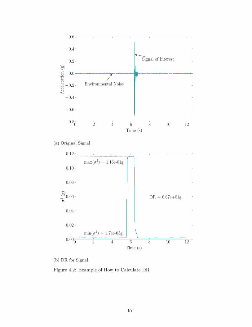
0 2 4 6 8 10 12Time (s)
−0.8
−0.6
−0.4
−0.2
0.0
0.2
0.4
0.6
Acce
lerat
ion
(g)
Environmental Noise
Signal of Interest
(a) Original Signal
0 2 4 6 8 10 12Time (s)
0.00
0.02
0.04
0.06
0.08
0.10
0.12
σ‡
(g)
max(σ‡) = 1.16e-01g
min(σ‡) = 1.74e-03g
DR = 6.67e+01g
(b) DR for Signal
Figure 4.2: Example of How to Calculate DR
67

SVMs can use many kernel functions for designing boundaries with the train-
ing data [26, 32]. The four kernels tested were linear, radial basis function (RBF),
polynomial (3rd degree), and sigmoid. The RBF outperformed the other kernels in
robustness, and had the most highest scoring best training sets (see Section 4.4).
The linear kernel came in second place in both aspects considered. Therefore, the
following discussion is presented with the linear and RBF.
The linear kernel is described by
K (x, x′) = x · x′ (4.10)
where x′ is the training and x is the testing data. The RBF is described by
K (x, x′) = e−γ|x−x′|2 (4.11)
where x′ and x represent the training and testing data respectively. These are
regulated by the shape parameter γ [26, 32, 33]. This “projects data from a low-
dimensional space to a space of higher dimension” [31] which increases the ability
of the SVM to determine decision boundaries, and thus increase the accuracy of
classification.
Kernels are fed into a decision function having the form of
f (x) = sign(
n∑i=1
yiαiK (x, x′) + ρ
)(4.12)
where sign () is the function described by Equation 4.13, x is the data to be classified, n
is the number of points of x, yi is a vector of form y ∈ {−1, 1}n, αi is the regularization
parameter in the range of 0 ≤ αi ≤ C with C being the penalty parameter, K (x, x′)
is the kernel function, and ρ is an independent intercept parameter [32]. Python
package Scikit-Learn v0.16.1 provides SVM functions used here [32].
68

sign (x) =
−1 if x ≤ 0
0 if x = 0
1 if x ≥ 0
(4.13)
4.4 Filtering of Acceleration Signals
Metrics from Section 4.2 were generated for all the available data and saved into
a relational database for future access. Data was first filtered using MADr to ignore
signals with data caused by sensor malfunctions (MADr < 0.95) and the NaN Den-
sity metric to find complete signals (ρnan = 0), that being the signals not having
any missing data points. Researchers then randomly selected 200 signals from the
database without knowing the metric values. The signals were plotted and manually
categorized using the following categories shown in Table 4.1.
Table 4.1: Signal Categories
Category Description Count1 Exhibiting lots of noise with little to no data 1602 Some activity but indistinct peaks or shape 223 Distinct peaks or shape 18
In this way, the SVM can learn the categories assigned by the researcher. The
SVM would relate categories to metric values and be able to sort the remainder of
the 536,686 records of the database. Examples of the categories from Table 4.1 are
presented in Figure 4.3.
The Pareto Principle, a guideline often used in economics and has seen use in
computer science, was chosen to validate the method where the split of the data set
becomes 80% training and 20% validation [34]. Data was randomly split into the
training and validation categories using the Scikit-Learn function train_test_split()
69
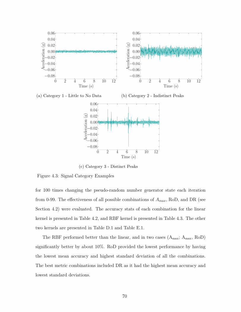
0 2 4 6 8 10 12Time (s)
−0.08−0.06−0.04−0.02
0.000.020.040.06
Acce
lerat
ion
(g)
(a) Category 1 - Little to No Data
0 2 4 6 8 10 12Time (s)
−0.08−0.06−0.04−0.02
0.000.020.040.06
Acce
lerat
ion
(g)
(b) Category 2 - Indistinct Peaks
0 2 4 6 8 10 12Time (s)
−0.08−0.06−0.04−0.02
0.000.020.040.06
Acce
lerat
ion
(g)
(c) Category 3 - Distinct Peaks
Figure 4.3: Signal Category Examples
for 100 times changing the pseudo-random number generator state each iteration
from 0-99. The effectiveness of all possible combinations of Amax, RoD, and DR (see
Section 4.2) were evaluated. The accuracy stats of each combination for the linear
kernel is presented in Table 4.2, and RBF kernel is presented in Table 4.3. The other
two kernels are presented in Table D.1 and Table E.1.
The RBF performed better than the linear, and in two cases (Amax; Amax, RoD)
significantly better by about 10%. RoD provided the lowest performance by having
the lowest mean accuracy and highest standard deviation of all the combinations.
The best metric combinations included DR as it had the highest mean accuracy and
lowest standard deviations.
70
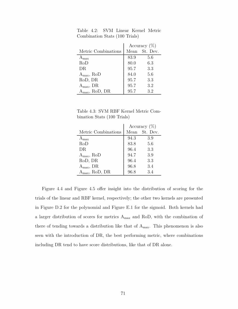
Table 4.2: SVM Linear Kernel MetricCombination Stats (100 Trials)
Accuracy (%)Metric Combinations Mean St. Dev.Amax 83.9 5.6RoD 80.0 6.3DR 95.7 3.3Amax, RoD 84.0 5.6RoD, DR 95.7 3.3Amax, DR 95.7 3.2Amax, RoD, DR 95.7 3.2
Table 4.3: SVM RBF Kernel Metric Com-bination Stats (100 Trials)
Accuracy (%)Metric Combinations Mean St. Dev.Amax 94.3 3.9RoD 83.8 5.6DR 96.4 3.3Amax, RoD 94.7 3.9RoD, DR 96.4 3.3Amax, DR 96.8 3.4Amax, RoD, DR 96.8 3.4
Figure 4.4 and Figure 4.5 offer insight into the distribution of scoring for the
trials of the linear and RBF kernel, respectively; the other two kernels are presented
in Figure D.2 for the polynomial and Figure E.1 for the sigmoid. Both kernels had
a larger distribution of scores for metrics Amax and RoD, with the combination of
there of tending towards a distribution like that of Amax. This phenomenon is also
seen with the introduction of DR, the best performing metric, where combinations
including DR tend to have score distributions, like that of DR alone.
71
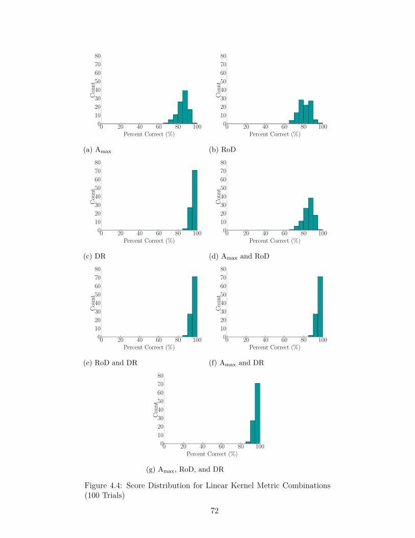
0 20 40 60 80 100Percent Correct (%)
01020304050607080
Coun
t
(a) Amax
0 20 40 60 80 100Percent Correct (%)
01020304050607080
Coun
t
(b) RoD
0 20 40 60 80 100Percent Correct (%)
01020304050607080
Coun
t
(c) DR
0 20 40 60 80 100Percent Correct (%)
01020304050607080
Coun
t
(d) Amax and RoD
0 20 40 60 80 100Percent Correct (%)
01020304050607080
Coun
t
(e) RoD and DR
0 20 40 60 80 100Percent Correct (%)
01020304050607080
Coun
t
(f) Amax and DR
0 20 40 60 80 100Percent Correct (%)
01020304050607080
Coun
t
(g) Amax, RoD, and DR
Figure 4.4: Score Distribution for Linear Kernel Metric Combinations(100 Trials)
72
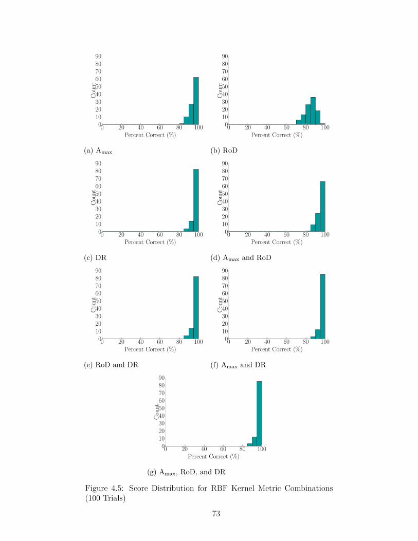
0 20 40 60 80 100Percent Correct (%)
0102030405060708090
Coun
t
(a) Amax
0 20 40 60 80 100Percent Correct (%)
0102030405060708090
Coun
t
(b) RoD
0 20 40 60 80 100Percent Correct (%)
0102030405060708090
Coun
t
(c) DR
0 20 40 60 80 100Percent Correct (%)
0102030405060708090
Coun
t
(d) Amax and RoD
0 20 40 60 80 100Percent Correct (%)
0102030405060708090
Coun
t
(e) RoD and DR
0 20 40 60 80 100Percent Correct (%)
0102030405060708090
Coun
t
(f) Amax and DR
0 20 40 60 80 100Percent Correct (%)
0102030405060708090
Coun
t
(g) Amax, RoD, and DR
Figure 4.5: Score Distribution for RBF Kernel Metric Combinations(100 Trials)
73
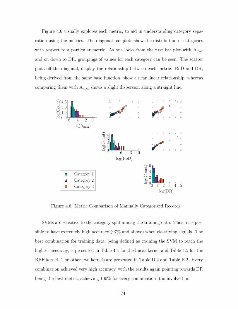
Figure 4.6 visually explores each metric, to aid in understanding category sepa-
ration using the metrics. The diagonal bar plots show the distribution of categories
with respect to a particular metric. As one looks from the first bar plot with Amax
and on down to DR, groupings of values for each category can be seen. The scatter
plots off the diagonal, display the relationship between each metric. RoD and DR,
being derived from the same base function, show a near linear relationship; whereas
comparing them with Amax shows a slight dispersion along a straight line.
−6 −4 −2 0log(Amax)
0.01.53.04.5
log(
Coun
t)
−9 −6 −3 0log(RoD)
01234
log(
Coun
t)
0 1 2 3 4 5log(DR)
0246
log(
Coun
t)
Category 1Category 2Category 3
Figure 4.6: Metric Comparison of Manually Categorized Records
SVMs are sensitive to the category split among the training data. Thus, it is pos-
sible to have extremely high accuracy (97% and above) when classifying signals. The
best combination for training data, being defined as training the SVM to reach the
highest accuracy, is presented in Table 4.4 for the linear kernel and Table 4.5 for the
RBF kernel. The other two kernels are presented in Table D.2 and Table E.2. Every
combination achieved very high accuracy, with the results again pointing towards DR
being the best metric, achieving 100% for every combination it is involved in.
74

Table 4.4: SVM Linear Kernel Best Training Set for EachMetric Combination
Metric Combinations C1 C2 C3 Accuracy (%)Amax 121 21 18 97.5RoD 121 21 18 97.5DR 129 18 13 100.0Amax, RoD 121 21 18 97.5RoD, DR 129 18 13 100.0Amax, DR 129 18 13 100.0Amax, RoD, DR 129 18 13 100.0
Table 4.5: SVM RBF Kernel Best Training Set for EachMetric Combination
Metric Combinations C1 C2 C3 Accuracy (%)Amax 121 21 18 100.0RoD 121 21 18 97.5DR 128 18 14 100.0Amax, RoD 121 21 18 100.0RoD, DR 128 18 14 100.0Amax, DR 128 18 14 100.0Amax, RoD, DR 128 18 14 100.0
Table 4.6 and Table 4.7 display the worst scoring category split observed during
the trials for the linear and RBF kernels, respectively. The remaining two kernels are
presented in Table D.3 and Table E.3. From these results, one can further see the
robustness of each metric for the SVM to better determine the hyperplanes between
categories.
Table 4.6: SVM Linear Kernel Worst Training Set forEach Metric Combination
Metric Combinations C1 C2 C3 Accuracy (%)Amax 134 11 15 67.5RoD 134 15 11 65.0DR 131 15 14 87.5Amax, RoD 134 11 15 67.5RoD, DR 131 15 14 87.5Amax, DR 131 15 14 87.5Amax, RoD, DR 131 15 14 87.5
75
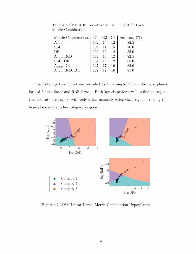
Table 4.7: SVM RBF Kernel Worst Training Set for EachMetric Combination
Metric Combinations C1 C2 C3 Accuracy (%)Amax 132 16 12 82.5RoD 134 11 15 70.0DR 132 16 12 85.0Amax, RoD 132 16 12 82.5RoD, DR 132 16 12 85.0Amax, DR 127 17 16 85.0Amax, RoD, DR 127 17 16 85.0
The following two figures are provided as an example of how the hyperplanes
formed for the linear and RBF kernels. Both kernels perform well in finding regions
that indicate a category, with only a few manually categorized signals crossing the
hyperplane into another category’s region.
−9 −7 −5 −3 −1log(RoD)
−6−5−4−3−2−1
01
log(
Am
ax)
0 1 2 3 4 5log(DR)
−9
−7
−5
−3
−1
log(
RoD
)
Category 1Category 2Category 3
Figure 4.7: SVM Linear Kernel Metric Combination Hyperplanes
76

−9 −7 −5 −3 −1log(RoD)
−6−5−4−3−2−1
01
log(
Am
ax)
0 1 2 3 4 5log(DR)
−9
−7
−5
−3
−1
log(
RoD
)
Category 1Category 2Category 3
Figure 4.8: SVM RBF Kernel Metric Combination Hyperplanes
4.5 Conclusion
At the time of this writing, the SVM, using the DR metric, has worked through
all 536,686 acceleration records much faster than if the same records were processed
manually. Preprocessing removed 273,422 records that were missing data points or
were identified as sensor malfunctions. This leaves 203,964 records in category one;
33,972 in category two; 25,321 in category three; and 7 records ignored as the value
of DR was infinity indicating a signal containing all the same value, something that
could also be filtered out in preprocessing in the future. Examples of SVM classified
signals are seen in Figure 4.9. Relatively few manually classified training samples are
required for the SVM to learn from, making this a very time-efficient method not
requiring much user input. In the case of this study, only 200 signals were used for
training - a mere 0.04% of the entire dataset.
77
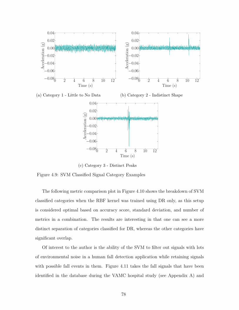
0 2 4 6 8 10 12Time (s)
−0.08
−0.06
−0.04
−0.02
0.00
0.02
0.04
Acce
lerat
ion
(g)
(a) Category 1 - Little to No Data
0 2 4 6 8 10 12Time (s)
−0.08
−0.06
−0.04
−0.02
0.00
0.02
0.04
Acce
lerat
ion
(g)
(b) Category 2 - Indistinct Shape
0 2 4 6 8 10 12Time (s)
−0.08
−0.06
−0.04
−0.02
0.00
0.02
0.04
Acce
lerat
ion
(g)
(c) Category 3 - Distinct Peaks
Figure 4.9: SVM Classified Signal Category Examples
The following metric comparison plot in Figure 4.10 shows the breakdown of SVM
classified categories when the RBF kernel was trained using DR only, as this setup
is considered optimal based on accuracy score, standard deviation, and number of
metrics in a combination. The results are interesting in that one can see a more
distinct separation of categories classified for DR, whereas the other categories have
significant overlap.
Of interest to the author is the ability of the SVM to filter out signals with lots
of environmental noise in a human fall detection application while retaining signals
with possible fall events in them. Figure 4.11 takes the fall signals that have been
identified in the database during the VAMC hospital study (see Appendix A) and
78
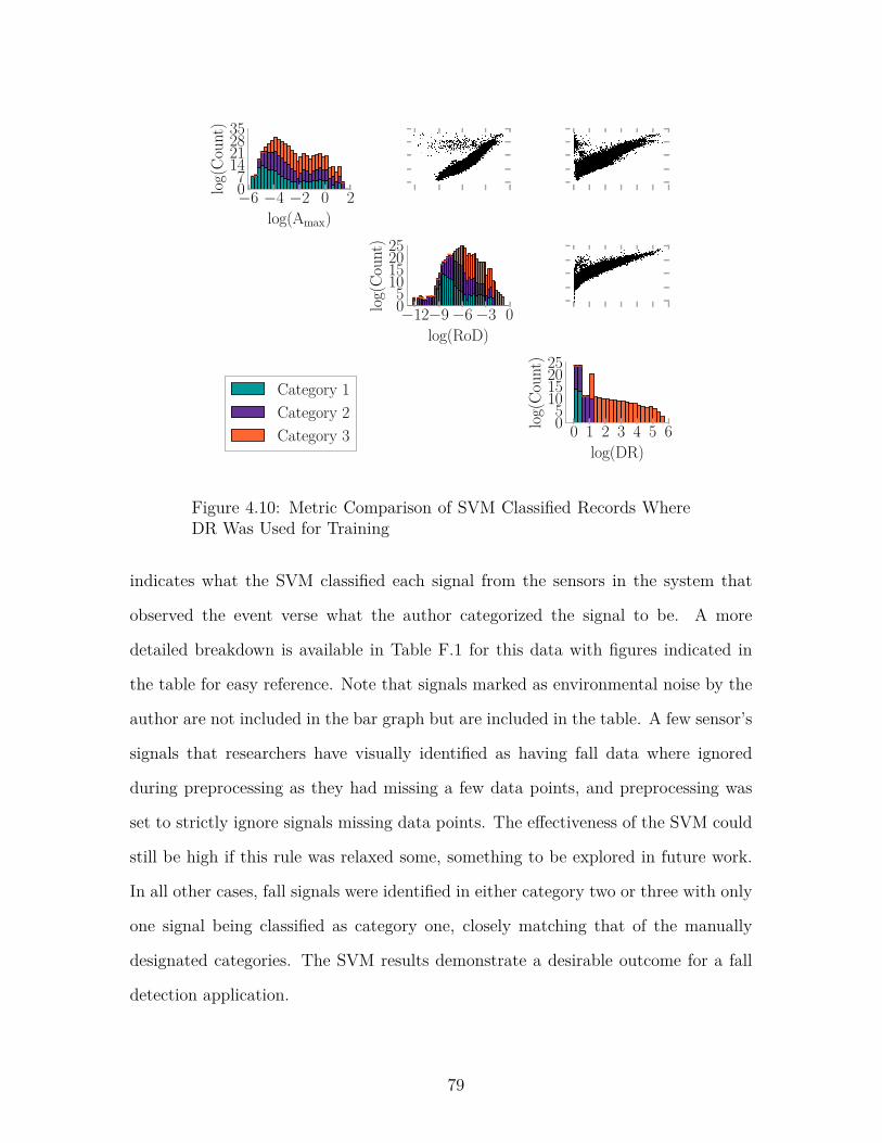
−6 −4 −2 0 2log(Amax)
07
14212835
log(
Coun
t)
−12−9 −6 −3 0log(RoD)
05
10152025
log(
Coun
t)
0 1 2 3 4 5 6log(DR)
05
10152025
log(
Coun
t)
Category 1Category 2Category 3
Figure 4.10: Metric Comparison of SVM Classified Records WhereDR Was Used for Training
indicates what the SVM classified each signal from the sensors in the system that
observed the event verse what the author categorized the signal to be. A more
detailed breakdown is available in Table F.1 for this data with figures indicated in
the table for easy reference. Note that signals marked as environmental noise by the
author are not included in the bar graph but are included in the table. A few sensor’s
signals that researchers have visually identified as having fall data where ignored
during preprocessing as they had missing a few data points, and preprocessing was
set to strictly ignore signals missing data points. The effectiveness of the SVM could
still be high if this rule was relaxed some, something to be explored in future work.
In all other cases, fall signals were identified in either category two or three with only
one signal being classified as category one, closely matching that of the manually
designated categories. The SVM results demonstrate a desirable outcome for a fall
detection application.
79
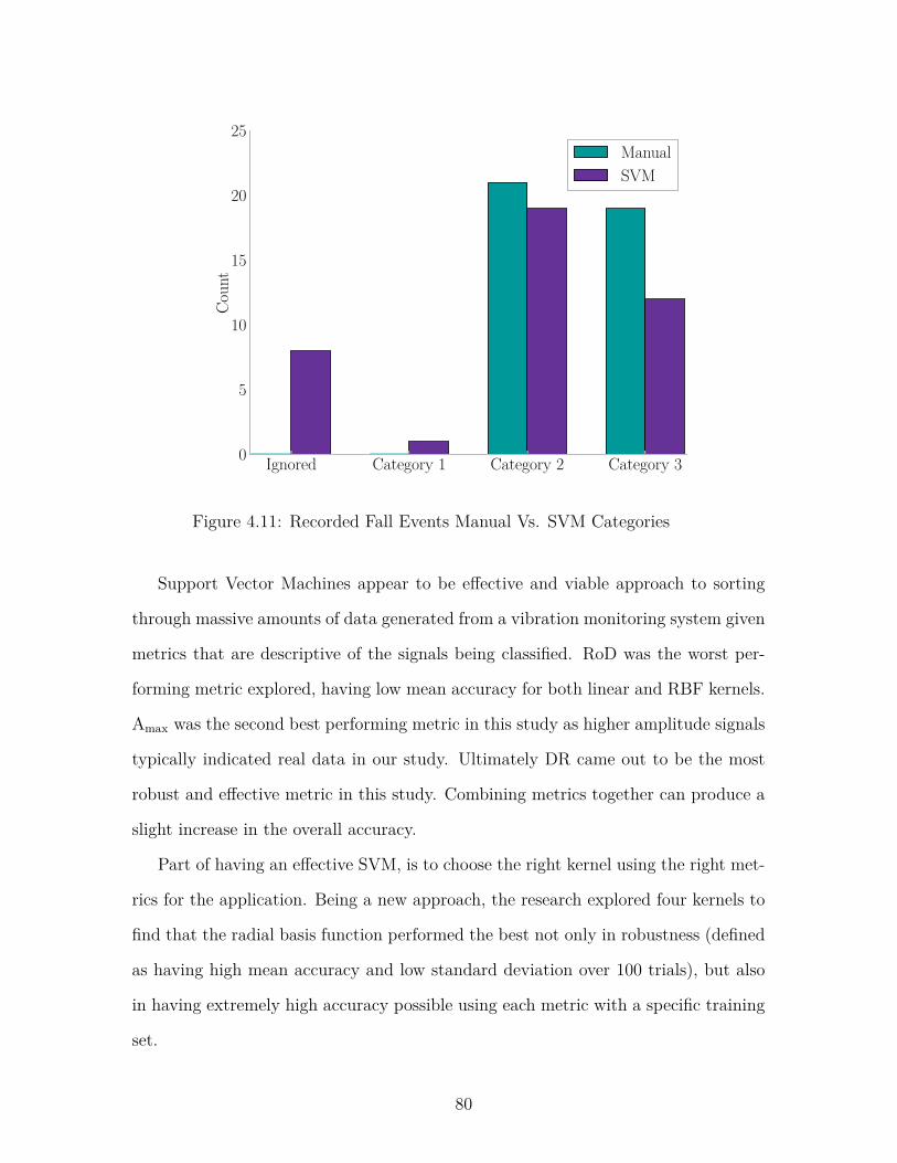
Ignored Category 1 Category 2 Category 30
5
10
15
20
25
Coun
t
ManualSVM
Figure 4.11: Recorded Fall Events Manual Vs. SVM Categories
Support Vector Machines appear to be effective and viable approach to sorting
through massive amounts of data generated from a vibration monitoring system given
metrics that are descriptive of the signals being classified. RoD was the worst per-
forming metric explored, having low mean accuracy for both linear and RBF kernels.
Amax was the second best performing metric in this study as higher amplitude signals
typically indicated real data in our study. Ultimately DR came out to be the most
robust and effective metric in this study. Combining metrics together can produce a
slight increase in the overall accuracy.
Part of having an effective SVM, is to choose the right kernel using the right met-
rics for the application. Being a new approach, the research explored four kernels to
find that the radial basis function performed the best not only in robustness (defined
as having high mean accuracy and low standard deviation over 100 trials), but also
in having extremely high accuracy possible using each metric with a specific training
set.
80

Chapter 5
The FEEL Algorithm
5.1 Introduction
An important part for treatment and rescue pertaining to fall detection is estimat-
ing the magnitude of the impact and its location within the structure. Doctors could
utilize the force information to determine the severity of injuries and take appropri-
ate action to prevent further exacerbation. Diagnosis and treatment of injuries thus
have the potential to be quicker with the impact’s force magnitude. Rescuers can use
the impact location information to more quickly find the fallen person, a useful tool
particularly when the fallen cannot yell for help. In addition, the force estimate can
also be used to differentiate between a person falling and objects being dropped.
The challenges of current state-of-the-art fall detection algorithms using structural
vibrations (discussed in Section 1.2) stem from the estimation of properties that vary
by structure (e.g. energy methods use structural damping estimations). Even with
ample experimentation and modeling of a structural system, the physical properties,
such as stiffness and damping, are still challenging to obtain. Thus, an algorithm
using floor vibrations should intrinsically embed within itself the attributes of any
structure.
5.2 Force Estimation and Event Localization (FEEL) Algorithm
The FEEL Algorithm was designed to intrinsically embed structural properties
into transfer function estimates between calibrated locations and sensors. Forces
81

and the dynamic response of the structure are related during the calibration process,
which eliminates challenges with distance between a sensor and an impact’s location
assuming the response is measurable. Time synchronization of sensors can be difficult,
thus FEEL was designed to not require it. The algorithm becomes more easily scalable
because of this. Scalability also brings with it greater robustness as more sensors can
be added to the mix to provide more information. A minimum of two sensors are
required to apply FEEL due to the pair matching method for estimating the location
and force of impact. FEEL has been implemented as the Python package feel with
documentation being provided in Appendix N and has been filed as U.S. Patent
Application No. 62/324,468 [35]. The process diagram for navigating the algorithm’s
operation is shown in Figure 5.1, with more detail on each step provided in the
following sections.
CalibrateT̂i,j
CaptureVibrations
EstimateForces{F̂i,j}
LocalizeEvent L̂
EstimateForce Mag-nitude F̂
Figure 5.1: FEEL Algorithm Process Diagram
5.2.1 Calibration
The FEEL Algorithm works by first dynamically characterizing the structure.
Calibration yields transfer functions between forces at plausible fall locations and
accelerations at the sensor locations. Force records obtained from an impulse hammer
and the resulting floor vibrations are recorded for use in the transfer function estimate
presented in Equation 5.1
T̂(f) = Txy(f) + Tyx(f)2 (5.1)
82
where
Txy(f) = Pxy(f)Pxx(f) (5.2)
Tyx(f) = Pyy(f)Pyx(f) (5.3)
x is input (force), y is output (accelerations), Pxy(f) is the cross power spectral
density of x to y, Pxx(f) is the power spectral density of x, Pyy(f) is the power
spectral density of y, and Pyx(f) is the cross power spectral density of y to x [36, 37].
The averaging of Txy(f) and Tyx(f) reduces the amount of noise and measurement
error present in the transfer function estimate.
5.2.2 Force Estimation
To estimate the force, one takes the acceleration signal S and applies the T̂(f) for
the each location of impact as seen in the following
[Ii,j] = FFT(S)[T̂i,j(f)
] (5.4)
[F̂i,j
]= IFFT ([Ii,j]) (5.5)
where FFT() is the Fast Fourier Transform, IFFT() is the Inverse Fast Fourier Trans-
form,[F̂i,j
]is the force estimation matrix, i is the location, and j is the sensor.
5.2.3 Event Localization
The location of events in other disciplines has traditionally been treated as a
‘time of flight’ problem. Sensors are time synchronized and the difference between
83

the arrival of a wave is used for localization [38, 39]. This technique has proven
successful in other areas of engineering but has significant challenges. In particular,
the sensors need to be synchronized and the wave speed needs to be known. This
would increase the complexity of the sensing system, and ultimately the potential
cost of production. Therefore, the author aimed at developing a method that does
not depend on time. The method compares force estimates for different locations
using data from different sensors. The location that estimates the same force, likely
corresponds to the location of impact.
The FEEL Algorithm event localization requires at least two sensors. The author
attempted many methods to compare the force estimates and found the use of the
Correlated Force Estimates Method to be the most robust due to its redundancy,
with reliability increasing with the more sensors used. Other techniques explored
during the development of the FEEL Algorithm are presented in Appendix G.
Correlated Force Estimates Method
The method begins by determining the window of the force estimation to consider
based on the maximum amplitude within the acceleration window. Alternatively, one
could use a threshold crossing method to choose a window within the force estimate,
like taking the time where the signal first crosses out of a ‘noise’ level previously
defined.
Symmetrical or asymmetrical windows may be used. The windows may also be
taken on a per sensor basis, by choosing one sensor as a reference and using its
window for all the sensors, or any combination thereof. The author suggests using
a symmetrical window and using one sensor as a reference. This is due to the fact
that the FEEL Algorithm is time-independent, meaning the force estimates at each
sensor will show peaks at the same time across all estimates, and the method is based
on the shape of the peak in the force estimates, making a symmetrical window ideal
84
for capturing the similarity of symmetrical peaks. The force estimates do usually
maintain a similar shape at the location of impact, which lends localization towards
this method.
After portions of each force estimate are selected, the normalized correlation co-
efficient matrix is formed using only the real portion of the force estimate like in
Equation 5.6
{Li} = max
0 ρxy(F̂i,1(n), F̂i,2(n)) · · · ρxy(F̂i,1(n), F̂i,j(n))
0 · · · ρxy(F̂i,2(n), F̂i,j(n)). . . ...
sym. 0
(5.6)
where
ρxy = COV (x, y)√
σxσy
(5.7)
is the Pearson product-moment correlation coefficient, cov() is the covariance, σ is the
standard deviation, x and y are vectors, {Li} is the vector of maximum normalized
correlation coefficient for each location i, max() is the maximum value function, F̂i,j
is the force estimation of the i-th location at the j-th sensor, and n is the number of
points in the window [21, 40].
The normalized correlation coefficients are then compared by location with the
largest value being the location of impact as in Equation 5.8 where L̂ is the highest
correlation coefficient, and max() is the maximum value function.
L̂ = max({Li}) (5.8)
85

The advantage of this approach stems from the pair matching in the correlation
matrix. Each force estimate is compared to the other, providing redundancy when
more sensors and consequently, more force estimates are available. There may be
times when very poor force estimates appear, so by taking the best pair of estimates
(i.e. the pair having the highest correlation value), error in locating the impact reduce
greatly. Furthermore, the acceleration records do not have to be time-synchronized,
reducing the complexity of the data acquisition system. The Correlated Force Esti-
mates Method thus provided the more robust localization of the methods tested.
5.2.4 Force Magnitude Estimation
Once the location has been identified as in Section 5.2.3, the two closest matching
pair of force vectors are used to estimate the force magnitude. The estimation of the
force can be biased with a constant value in the acceleration measurements. Yet, the
force magnitude estimate of the i-th location and j-th sensor can be estimated using
F̂i,j = max({F̂i,j}
)− min
({F̂i,j}
)(5.9)
where max() is the maximum value function, {F̂i,j} is the real portion of the force
estimation vector produced by Equation 5.5, and min() is the minimum value func-
tion. Figure 5.2 demonstrates a biased force estimation. Applying Equation 5.9, one
can see the accuracy of the force magnitude estimate increases for the location and
sensor.
The force magnitude for the specific acceleration event is taken to be the average
of the two sensor’s force estimation magnitudes whose force estimation vectors more
closely match as seen in Equation 5.10
F̂ = F̂i,1 + F̂i,2
2 (5.10)
86
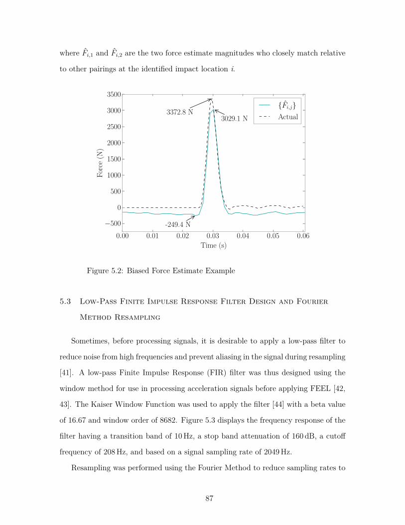
where F̂i,1 and F̂i,2 are the two force estimate magnitudes who closely match relative
to other pairings at the identified impact location i.
0.00 0.01 0.02 0.03 0.04 0.05 0.06Time (s)
−500
0
500
1000
1500
2000
2500
3000
3500Fo
rce
(N)
-249.4 N
3029.1 N3372.8 N
{F̂i,j}Actual
Figure 5.2: Biased Force Estimate Example
5.3 Low-Pass Finite Impulse Response Filter Design and Fourier
Method Resampling
Sometimes, before processing signals, it is desirable to apply a low-pass filter to
reduce noise from high frequencies and prevent aliasing in the signal during resampling
[41]. A low-pass Finite Impulse Response (FIR) filter was thus designed using the
window method for use in processing acceleration signals before applying FEEL [42,
43]. The Kaiser Window Function was used to apply the filter [44] with a beta value
of 16.67 and window order of 8682. Figure 5.3 displays the frequency response of the
filter having a transition band of 10 Hz, a stop band attenuation of 160 dB, a cutoff
frequency of 208 Hz, and based on a signal sampling rate of 2049 Hz.
Resampling was performed using the Fourier Method to reduce sampling rates to
87

0 200 400 600 800 1000Frequency (Hz)
0.0
0.2
0.4
0.6
0.8
1.0
Gai
n
Figure 5.3: Low-Pass FIR Filter Frequency Response
400 Hz after the filter was applied to the data [21, 45]. A signal delay was calculated
using Equation 5.11 where N is the number of coefficients in the filter, d is the number
of data points in the delay, FSnew is the new sampling rate, and FSold is the original
sample rate of the signal [21].
d =(
N − 12
)(FSnew
FSold
)(5.11)
The above signal delay equations give the number of samples the filtering process
have been affected by the filter’s initial conditions, and it is suggested to round the
values if a whole number is not produced from the equations. To get the amount
of time the signal delay equates to, use Equation 5.12 where d is the signal delay
calculated in Equation 5.11.
∆t = d
FSnew
(5.12)
88

The filter and resampling mentioned here are both provided in the feel Python
package for convenient use. See Appendix N for more details.
5.4 Verification Experiments
The FEEL Algorithm was tested on a small scale steel structure at the Structural
Dynamics and Intelligent Infrastructure Laboratory (SDII) at the University of South
Carolina (USC) in two trials. The structure is shown in Figure 5.4 and was built using
3.18 cm (1.25 in) outer diameter, 0.478 cm (0.188 in) wall DOM cold-rolled tube steel
as the beams and 2.54 cm (1 in) NC 2C threaded rods to connect the beams to the
6.35 cm (2.5 in) cubic 1018 cold-rolled bar. The tubes and cubes were thread in an
20.32 cm (8 in) pitch. The structure is suspended on steel supports and allowed to
rotate around the horizontal axis using mounted bearings. Even though the dynamic
characteristics of the structure do not match those of a residential dwelling, the
objective of the tests described here is to verify if the algorithm would work before
moving to a full scale structure. Three PCB Piezotronics 333B50 accelerometers with
a sensitivity of 1000 mV/g were attached to the structure using magnetic mounts at
nodes 8, 9, and 12. A 2.22 N (0.5 lb) PCB Piezotronics Impulse Force Hammer having
a sensitivity of 2.33 mV/N (10.35 mV/lb) was used to excite the structure,. Data was
collected at a rate of 2049 Hz, filtered using a FIR, and downsampled to 400 Hz as in
Section 5.3. The lower rate was chosen in order to model a more realistic scenario.
5.4.1 Preliminary Trial
The first trial served to indicate the viability of the FEEL Algorithm. Transfer
functions were calculated using the method outlined in Section 5.2.1 at node 7 (Fig-
ure 5.5) and node 10 (Figure 5.6) for all three sensors using a nfft value of 2048 and
a noverlap value of 1024. The data used for the transfer functions was captured in one
continuous record containing forces and accelerations. Five impacts were performed,
89

1 2 3 4
5 6 7 8
9 10 11 12
13 14 15 16
40.5 cm 40.5 cm 40.5 cm
68.5
8cm
68.5
8cm
68.5
8cm
Sensor 1
Sensor 2 Sensor 3
Figure 5.4: Steel Test Frame Layout
with the structure being allowed to return to rest after each hammer hit.
The transfer functions were then used to estimate the force of impact using the
method in Section 5.2.2. Figure 5.7 displays the node 7 impact results, and Figure 5.8
displays the node 10 impact results. The force estimations for both impacts were used
to identify the location of an impact based on the Correlated Force Estimates Method
in Section 5.2.3. The location results for node 7’s impact are displayed in Figure 5.9,
and node 10’s impact displayed in Figure 5.10. The correct location is highlighted in
orange. The force magnitude was calculated as in Section 5.2.4 and results displayed
in Table 5.1. FEEL was successful in identifying the location and force of the impacts.
90

0 50 100 150 200Frequency (Hz)
−90
−80
−70
−60
−50
−40
−30
−20
−10
Powe
r(dB
)
Sensor 1Sensor 2Sensor 3
Figure 5.5: T̂7,j for j From 1 to 3
0 50 100 150 200Frequency (Hz)
−90
−80
−70
−60
−50
−40
−30
−20
−10
Powe
r(dB
)
Sensor 1Sensor 2Sensor 3
Figure 5.6: T̂10,j for j From 1 to 3
91

0.00 0.02 0.04 0.06 0.08 0.10 0.12 0.14Time (s)
−10
0
10
20
30
40
50
60
70
80
Forc
e(N
)
Sensor 1Sensor 2Sensor 3Actual
(a) F̂7,j
0.00 0.02 0.04 0.06 0.08 0.10 0.12 0.14Time (s)
−10
0
10
20
30
40
50
60
70
80
Forc
e(N
)
Sensor 1Sensor 2Sensor 3Actual
(b) F̂10,j
Figure 5.7: Force Estimations for an Impact on Node 7
92

0.00 0.02 0.04 0.06 0.08 0.10 0.12 0.14Time (s)
0
20
40
60
80
100
Forc
e(N
)
Sensor 1Sensor 2Sensor 3Actual
(a) F̂7,j
0.00 0.02 0.04 0.06 0.08 0.10 0.12 0.14Time (s)
0
20
40
60
80
100
Forc
e(N
)
Sensor 1Sensor 2Sensor 3Actual
(b) F̂10,j
Figure 5.8: Force Estimations for an Impact on Node 10
93
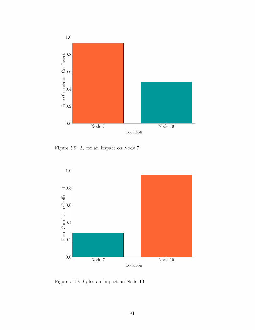
Node 7 Node 10Location
0.0
0.2
0.4
0.6
0.8
1.0
Forc
eCo
rrela
tion
Coeffi
cient
Figure 5.9: Li for an Impact on Node 7
Node 7 Node 10Location
0.0
0.2
0.4
0.6
0.8
1.0
Forc
eCo
rrela
tion
Coeffi
cient
Figure 5.10: Li for an Impact on Node 10
94
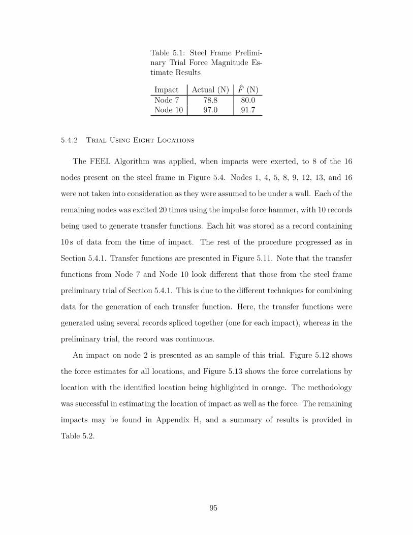
Table 5.1: Steel Frame Prelimi-nary Trial Force Magnitude Es-timate Results
Impact Actual (N) F̂ (N)Node 7 78.8 80.0Node 10 97.0 91.7
5.4.2 Trial Using Eight Locations
The FEEL Algorithm was applied, when impacts were exerted, to 8 of the 16
nodes present on the steel frame in Figure 5.4. Nodes 1, 4, 5, 8, 9, 12, 13, and 16
were not taken into consideration as they were assumed to be under a wall. Each of the
remaining nodes was excited 20 times using the impulse force hammer, with 10 records
being used to generate transfer functions. Each hit was stored as a record containing
10 s of data from the time of impact. The rest of the procedure progressed as in
Section 5.4.1. Transfer functions are presented in Figure 5.11. Note that the transfer
functions from Node 7 and Node 10 look different that those from the steel frame
preliminary trial of Section 5.4.1. This is due to the different techniques for combining
data for the generation of each transfer function. Here, the transfer functions were
generated using several records spliced together (one for each impact), whereas in the
preliminary trial, the record was continuous.
An impact on node 2 is presented as an sample of this trial. Figure 5.12 shows
the force estimates for all locations, and Figure 5.13 shows the force correlations by
location with the identified location being highlighted in orange. The methodology
was successful in estimating the location of impact as well as the force. The remaining
impacts may be found in Appendix H, and a summary of results is provided in
Table 5.2.
95

0 50 100 150 200Frequency (Hz)
−270
−254
−238
−222
−206
−190
Powe
r(dB
)
Sensor 1Sensor 2Sensor 3
(a) T̂14,j
0 50 100 150 200Frequency (Hz)
−270
−254
−238
−222
−206
−190
Powe
r(dB
)
Sensor 1Sensor 2Sensor 3
(b) T̂15,j
0 50 100 150 200Frequency (Hz)
−270
−254
−238
−222
−206
−190
Powe
r(dB
)
Sensor 1Sensor 2Sensor 3
(c) T̂10,j
0 50 100 150 200Frequency (Hz)
−270
−254
−238
−222
−206
−190
Powe
r(dB
)
Sensor 1Sensor 2Sensor 3
(d) T̂11,j
0 50 100 150 200Frequency (Hz)
−270
−254
−238
−222
−206
−190
Powe
r(dB
)
Sensor 1Sensor 2Sensor 3
(e) T̂6,j
0 50 100 150 200Frequency (Hz)
−270
−254
−238
−222
−206
−190
Powe
r(dB
)
Sensor 1Sensor 2Sensor 3
(f) T̂7,j
0 50 100 150 200Frequency (Hz)
−270
−254
−238
−222
−206
−190
Powe
r(dB
)
Sensor 1Sensor 2Sensor 3
(g) T̂2,j
0 50 100 150 200Frequency (Hz)
−270
−254
−238
−222
−206
−190
Powe
r(dB
)
Sensor 1Sensor 2Sensor 3
(h) T̂3,j
Figure 5.11: Steel Frame Transfer Functions
96
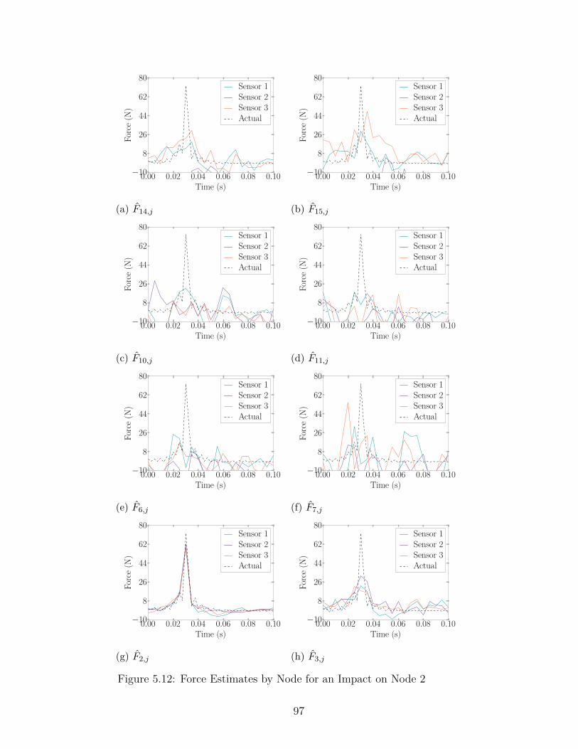
0.00 0.02 0.04 0.06 0.08 0.10Time (s)
−10
8
26
44
62
80
Forc
e(N
)
Sensor 1Sensor 2Sensor 3Actual
(a) F̂14,j
0.00 0.02 0.04 0.06 0.08 0.10Time (s)
−10
8
26
44
62
80
Forc
e(N
)
Sensor 1Sensor 2Sensor 3Actual
(b) F̂15,j
0.00 0.02 0.04 0.06 0.08 0.10Time (s)
−10
8
26
44
62
80
Forc
e(N
)
Sensor 1Sensor 2Sensor 3Actual
(c) F̂10,j
0.00 0.02 0.04 0.06 0.08 0.10Time (s)
−10
8
26
44
62
80
Forc
e(N
)
Sensor 1Sensor 2Sensor 3Actual
(d) F̂11,j
0.00 0.02 0.04 0.06 0.08 0.10Time (s)
−10
8
26
44
62
80
Forc
e(N
)
Sensor 1Sensor 2Sensor 3Actual
(e) F̂6,j
0.00 0.02 0.04 0.06 0.08 0.10Time (s)
−10
8
26
44
62
80
Forc
e(N
)
Sensor 1Sensor 2Sensor 3Actual
(f) F̂7,j
0.00 0.02 0.04 0.06 0.08 0.10Time (s)
−10
8
26
44
62
80
Forc
e(N
)
Sensor 1Sensor 2Sensor 3Actual
(g) F̂2,j
0.00 0.02 0.04 0.06 0.08 0.10Time (s)
−10
8
26
44
62
80
Forc
e(N
)
Sensor 1Sensor 2Sensor 3Actual
(h) F̂3,j
Figure 5.12: Force Estimates by Node for an Impact on Node 2
97

Node 2
Node 3
Node 6
Node 7
Node 10
Node 11
Node 14
Node 15
Location
0.0
0.2
0.4
0.6
0.8
1.0
Forc
eCo
rrela
tion
Coeffi
cient
Figure 5.13: Li for an Impact on Node 2
The results from the steel frame indicate the viability of the FEEL Algorithm.
Each impact set correctly identified the node the impact occurred on, and closely
estimated the maximum force of the impact. Sometimes a node near the impact,
such as node 2 in Figure H.1, shows some convergence of the three sensors. This
demonstrates that each transfer function has an area of influence, which will be
explored in future work.
Table 5.2: Steel Frame Trial Using EightLocations Results Summary
Impact L̂ Actual (N) F̂ (N)Node 2 Node 2 72.7 63.4Node 3 Node 3 13.6 10.7Node 6 Node 6 26.0 22.5Node 7 Node 7 88.4 83.9Node 10 Node 10 12.9 11.1Node 11 Node 11 18.0 19.0Node 14 Node 14 24.4 23.7Node 15 Node 15 38.5 29.6
98

5.5 Implementation Experiments
This section discusses the performance of the FEEL Algorithm in a full scale
structural environment based on the human-induced vibration benchmark dataset
developed by Arocha [46]. The experiments were performed in the second story office
of the USC Structures Laboratory, measuring 777 cm (25.5 ft) by 638 cm (20.9 ft),
that has reinforced concrete floors covered in vinyl tiles. The experimental layout
is presented in Figure 5.14. Three PCB Piezotronics 333B50 accelerometers with
sensitivity of 1000 mV/g were installed on the floor near the walls. Data was collected
at a rate of 1651.7 Hz with 2 s windows. Five locations were chosen on the floor for
the experiment. A total of 3575 impact events of eight different types were available.
The events include hammer impacts (Section 5.5.1), ball drops (Section 5.5.2), bag
Location 1
Location 2
Location 3
Location 4
Location 5Sensor1
Sensor 2
Sensor 3
Sensor 4
777 cm
638c
m
412c
m
282 cm
320 cm
389 cm
318c
m
310 cm
220c
m
171 cm
145c
m
218 cm
227c
m
239 cm
315c
m
120 cm
231c
m
Figure 5.14: Implementation Experimental Layout
99

drops (Section 5.5.3), and human jumps (Section 5.5.4). Event types are outline in
Table 5.3 and example acceleration records are provided in Figure 5.15.
Table 5.3: Implementation ExperimentEvent Types
Event Name Mass (kg) Detailshammer 5.49ball-low 0.56 1.42 m dropball-high 0.56 2.10 m dropbag-low 0.45 1.42 m dropbag-high 0.45 2.10 m dropd-jump 80 malej-jump 55 femalew-jump 85 male
5.5.1 Force Hammer Trials
Transfer functions were developed for each of the five locations (see Figure 5.16)
using a PCB Piezotronics Impulse Force Hammer Model 086D50 with a sensitivity of
0.2305 mV/N (1.025 mV/lb) and the ability to excite to a frequencies up to 800 Hz.
Five separate impacts were combined into one long force vector for calculation of
the transfer functions as seen in Figure 5.16. Then, 15 separate impacts per loca-
tion (total of 75 impacts) were used to validate the FEEL Algorithm. Results for a
single impact on location one are presented where Figure 5.15h displays the accel-
eration signals, Figure 5.17 displays force estimations, and Figure 5.18 displays the
force correlation coefficients with the identified location in orange. Examples for the
remaining locations are presented in Appendix I.
A histogram of the difference between the estimated force magnitudes and those
measured with the force hammer are shown in Figure 5.19, with a mean of 183.9 N
(41.3 lb) and a standard deviation of of 184.3 N (41.4 lb). The estimates largely tend
to be within 200 N (45 lb) of the measured force for each impact, with 72.0% of
estimates falling within this range. Figure 5.20 displays the distribution of the force
100
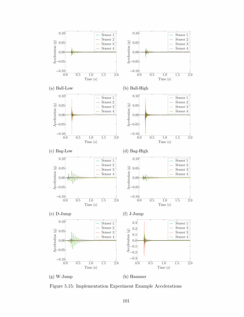
0.0 0.5 1.0 1.5 2.0Time (s)
−0.10
−0.05
0.00
0.05
0.10
Acce
lerat
ion
(g)
Sensor 1Sensor 2Sensor 3Sensor 4
(a) Ball-Low
0.0 0.5 1.0 1.5 2.0Time (s)
−0.10
−0.05
0.00
0.05
0.10
Acce
lerat
ion
(g)
Sensor 1Sensor 2Sensor 3Sensor 4
(b) Ball-High
0.0 0.5 1.0 1.5 2.0Time (s)
−0.10
−0.05
0.00
0.05
0.10
Acce
lerat
ion
(g)
Sensor 1Sensor 2Sensor 3Sensor 4
(c) Bag-Low
0.0 0.5 1.0 1.5 2.0Time (s)
−0.10
−0.05
0.00
0.05
0.10
Acce
lerat
ion
(g)
Sensor 1Sensor 2Sensor 3Sensor 4
(d) Bag-High
0.0 0.5 1.0 1.5 2.0Time (s)
−0.10
−0.05
0.00
0.05
0.10
Acce
lerat
ion
(g)
Sensor 1Sensor 2Sensor 3Sensor 4
(e) D-Jump
0.0 0.5 1.0 1.5 2.0Time (s)
−0.10
−0.05
0.00
0.05
0.10
Acce
lerat
ion
(g)
Sensor 1Sensor 2Sensor 3Sensor 4
(f) J-Jump
0.0 0.5 1.0 1.5 2.0Time (s)
−0.10
−0.05
0.00
0.05
0.10
Acce
lerat
ion
(g)
Sensor 1Sensor 2Sensor 3Sensor 4
(g) W-Jump
0.0 0.5 1.0 1.5 2.0Time (s)
−0.3−0.2−0.1
0.00.10.20.3
Acce
lerat
ion
(g)
Sensor 1Sensor 2Sensor 3Sensor 4
(h) Hammer
Figure 5.15: Implementation Experiment Example Accelerations
101

0 200 400 600 800Frequency (Hz)
−140
−110
−80
−50
−20
Powe
r(dB
)
Sensor 1Sensor 2Sensor 3Sensor 4
(a) T̂1,j
0 200 400 600 800Frequency (Hz)
−140
−110
−80
−50
−20
Powe
r(dB
)
Sensor 1Sensor 2Sensor 3Sensor 4
(b) T̂2,j
0 200 400 600 800Frequency (Hz)
−140
−110
−80
−50
−20
Powe
r(dB
)
Sensor 1Sensor 2Sensor 3Sensor 4
(c) T̂3,j
0 200 400 600 800Frequency (Hz)
−140
−110
−80
−50
−20
Powe
r(dB
)Sensor 1Sensor 2Sensor 3Sensor 4
(d) T̂4,j
0 200 400 600 800Frequency (Hz)
−140
−110
−80
−50
−20
Powe
r(dB
)
Sensor 1Sensor 2Sensor 3Sensor 4
(e) T̂5,j
Figure 5.16: Concrete Floor Transfer Functions
102
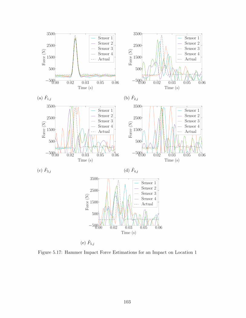
0.00 0.02 0.03 0.05 0.06Time (s)
−500
500
1500
2500
3500
Forc
e(N
)Sensor 1Sensor 2Sensor 3Sensor 4Actual
(a) F̂1,j
0.00 0.02 0.03 0.05 0.06Time (s)
−500
500
1500
2500
3500
Forc
e(N
)
Sensor 1Sensor 2Sensor 3Sensor 4Actual
(b) F̂2,j
0.00 0.02 0.03 0.05 0.06Time (s)
−500
500
1500
2500
3500
Forc
e(N
)
Sensor 1Sensor 2Sensor 3Sensor 4Actual
(c) F̂3,j
0.00 0.02 0.03 0.05 0.06Time (s)
−500
500
1500
2500
3500
Forc
e(N
)
Sensor 1Sensor 2Sensor 3Sensor 4Actual
(d) F̂4,j
0.00 0.02 0.03 0.05 0.06Time (s)
−500
500
1500
2500
3500
Forc
e(N
)
Sensor 1Sensor 2Sensor 3Sensor 4Actual
(e) F̂5,j
Figure 5.17: Hammer Impact Force Estimations for an Impact on Location 1
103
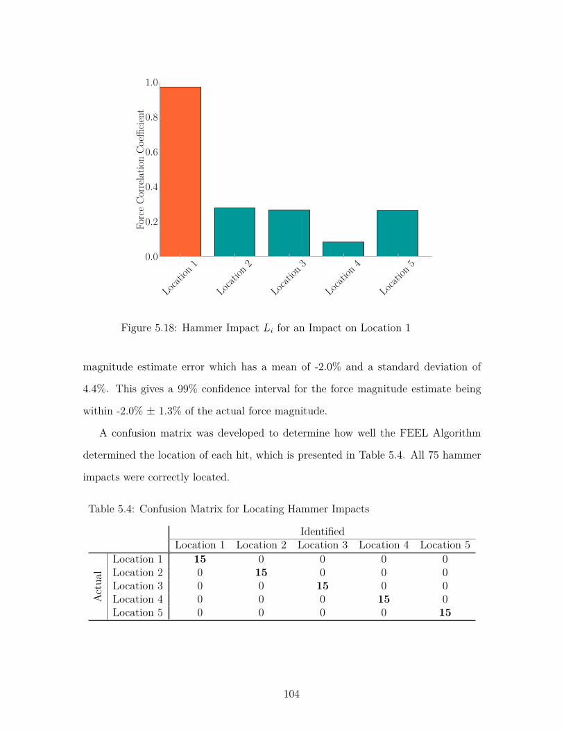
Locat
ion1
Locat
ion2
Locat
ion3
Locat
ion4
Locat
ion5
0.0
0.2
0.4
0.6
0.8
1.0
Forc
eCo
rrela
tion
Coeffi
cient
Figure 5.18: Hammer Impact Li for an Impact on Location 1
magnitude estimate error which has a mean of -2.0% and a standard deviation of
4.4%. This gives a 99% confidence interval for the force magnitude estimate being
within -2.0% ± 1.3% of the actual force magnitude.
A confusion matrix was developed to determine how well the FEEL Algorithm
determined the location of each hit, which is presented in Table 5.4. All 75 hammer
impacts were correctly located.
Table 5.4: Confusion Matrix for Locating Hammer Impacts
IdentifiedLocation 1 Location 2 Location 3 Location 4 Location 5
Act
ual
Location 1 15 0 0 0 0Location 2 0 15 0 0 0Location 3 0 0 15 0 0Location 4 0 0 0 15 0Location 5 0 0 0 0 15
104

0 200 400 600 800 1000Force Magnitude Difference (N)
0
5
10
15
20
25
30
35
40
Occ
urre
nces
Figure 5.19: Hammer Impacts Force Magnitude Estimation Differ-ence
−15 −10 −5 0 5 10Force Magnitude Error (%)
0
2
4
6
8
10
12
14
16
18
Occ
urre
nces
Figure 5.20: Hammer Impacts Force Magnitude Estimation Error
105

5.5.2 Ball Drop Trials
A basketball weighing 0.56 kg (1.23 lb) was dropped from two different heights at
each location for 100 repetitions. The trial named ball-low indicates a drop height
of 1.42 m (4.63 ft), and the trial named ball-high indicates a drop height of 2.10 m
(6.89 ft).
A sample impact for ball-low at location one is presented with Figure 5.15a show-
ing the vibrations the floor experienced, Figure 5.22 showing the force estimations at
each location, and Figure 5.21 showing the resulting correlation coefficients where the
orange bar is the identified location. Note that unlike with the hammer excitation,
no force record is available for comparison.
Locat
ion1
Locat
ion2
Locat
ion3
Locat
ion4
Locat
ion5
0.0
0.2
0.4
0.6
0.8
1.0
Forc
eCo
rrela
tion
Coeffi
cient
Figure 5.21: Ball-Low Li for an Impact on Location 1
A confusion matrix was generated to demonstrate the accuracy of the FEEL
Algorithm for location when the impact was caused by ball-low in Table 5.5. All 500
ball-low impacts were correctly identified giving a 100% success rate.
106

0.00 0.02 0.04 0.07 0.09Time (s)
−200
−40
120
280
440
600
Forc
e(N
)Sensor 1Sensor 2Sensor 3Sensor 4
(a) F̂1,j
0.00 0.02 0.04 0.07 0.09Time (s)
−200
−40
120
280
440
600
Forc
e(N
)
Sensor 1Sensor 2Sensor 3Sensor 4
(b) F̂2,j
0.00 0.02 0.04 0.07 0.09Time (s)
−200
−40
120
280
440
600
Forc
e(N
)
Sensor 1Sensor 2Sensor 3Sensor 4
(c) F̂3,j
0.00 0.02 0.04 0.07 0.09Time (s)
−200
−40
120
280
440
600
Forc
e(N
)
Sensor 1Sensor 2Sensor 3Sensor 4
(d) F̂4,j
0.00 0.02 0.04 0.07 0.09Time (s)
−200
−40
120
280
440
600
Forc
e(N
)
Sensor 1Sensor 2Sensor 3Sensor 4
(e) F̂5,j
Figure 5.22: Ball-Low Force Estimations for an Impact on Location 1
107

Table 5.5: Confusion Matrix for Locating Ball-Low Impacts
IdentifiedLocation 1 Location 2 Location 3 Location 4 Location 5
Act
ual
Location 1 100 0 0 0 0Location 2 0 100 0 0 0Location 3 0 0 100 0 0Location 4 0 0 0 100 0Location 5 0 0 0 0 100
A histogram of the estimated force magnitudes shown in Figure 5.23 demonstrates
a tight grouping of the force estimates around 500 N-600 N (123 lb-135 lb) having a
mean of 569.5 N (128.0 lb) and standard deviation of 41.3 N (11.5 lb). The variation
in estimates is due to how the ball drop experiment was performed as well as errors
in FEEL. The experiment was performed by a person holding and releasing the ball.
This means there will be some variation in the force as the person holds the ball at a
slightly different heights, and the ball bounces at slightly different spots each time.
400 450 500 550 600 650 700 750 800Force Magnitude Estimation (N)
0
50
100
150
200
Occ
urre
nces
Figure 5.23: Ball-Low Force Magnitude Estimation Histogram
108

A sample impact for ball-high at location four is presented with Figure 5.15b
showing the vibrations the floor experienced, Figure 5.25 showing the force estima-
tions at each location, and Figure 5.24 showing the resulting correlation coefficients
where the orange bar is the identified location.
Locat
ion1
Locat
ion2
Locat
ion3
Locat
ion4
Locat
ion5
0.0
0.2
0.4
0.6
0.8
1.0
Forc
eCo
rrela
tion
Coeffi
cient
Figure 5.24: Ball-High Li for an Impact on Location 1
A confusion matrix was generated to demonstrate the accuracy of the FEEL
Algorithm for localization in the case of ball-high in Table 5.6. Of the 500 ball-high
impacts, 499 were correctly identified which is a 99.8% success rate.
Table 5.6: Confusion Matrix for Locating Ball-High Impacts
IdentifiedLocation 1 Location 2 Location 3 Location 4 Location 5
Act
ual
Location 1 100 0 0 0 0Location 2 0 100 0 0 0Location 3 1 0 99 0 0Location 4 0 0 0 100 0Location 5 0 0 0 0 100
109
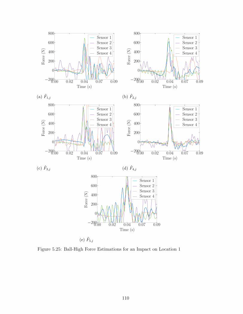
0.00 0.02 0.04 0.07 0.09Time (s)
−200
0
200
400
600
800
Forc
e(N
)Sensor 1Sensor 2Sensor 3Sensor 4
(a) F̂1,j
0.00 0.02 0.04 0.07 0.09Time (s)
−200
0
200
400
600
800
Forc
e(N
)
Sensor 1Sensor 2Sensor 3Sensor 4
(b) F̂2,j
0.00 0.02 0.04 0.07 0.09Time (s)
−200
0
200
400
600
800
Forc
e(N
)
Sensor 1Sensor 2Sensor 3Sensor 4
(c) F̂3,j
0.00 0.02 0.04 0.07 0.09Time (s)
−200
0
200
400
600
800
Forc
e(N
)
Sensor 1Sensor 2Sensor 3Sensor 4
(d) F̂4,j
0.00 0.02 0.04 0.07 0.09Time (s)
−200
0
200
400
600
800
Forc
e(N
)
Sensor 1Sensor 2Sensor 3Sensor 4
(e) F̂5,j
Figure 5.25: Ball-High Force Estimations for an Impact on Location 1
110
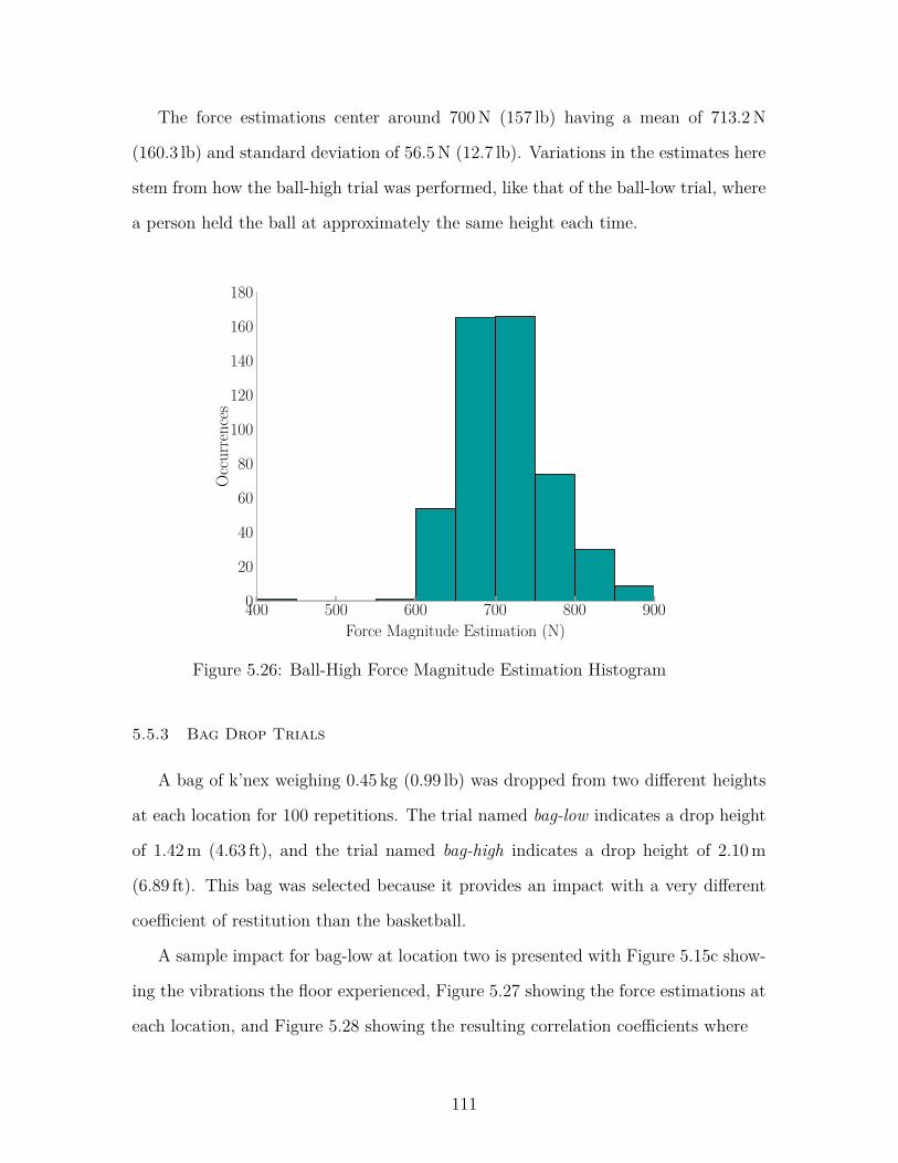
The force estimations center around 700 N (157 lb) having a mean of 713.2 N
(160.3 lb) and standard deviation of 56.5 N (12.7 lb). Variations in the estimates here
stem from how the ball-high trial was performed, like that of the ball-low trial, where
a person held the ball at approximately the same height each time.
400 500 600 700 800 900Force Magnitude Estimation (N)
0
20
40
60
80
100
120
140
160
180
Occ
urre
nces
Figure 5.26: Ball-High Force Magnitude Estimation Histogram
5.5.3 Bag Drop Trials
A bag of k’nex weighing 0.45 kg (0.99 lb) was dropped from two different heights
at each location for 100 repetitions. The trial named bag-low indicates a drop height
of 1.42 m (4.63 ft), and the trial named bag-high indicates a drop height of 2.10 m
(6.89 ft). This bag was selected because it provides an impact with a very different
coefficient of restitution than the basketball.
A sample impact for bag-low at location two is presented with Figure 5.15c show-
ing the vibrations the floor experienced, Figure 5.27 showing the force estimations at
each location, and Figure 5.28 showing the resulting correlation coefficients where
111

0.00 0.01 0.02 0.03 0.04Time (s)
−200
−80
40
160
280
400
Forc
e(N
)Sensor 1Sensor 2Sensor 3Sensor 4
(a) F̂1,j
0.00 0.01 0.02 0.03 0.04Time (s)
−200
−80
40
160
280
400
Forc
e(N
)
Sensor 1Sensor 2Sensor 3Sensor 4
(b) F̂2,j
0.00 0.01 0.02 0.03 0.04Time (s)
−200
−80
40
160
280
400
Forc
e(N
)
Sensor 1Sensor 2Sensor 3Sensor 4
(c) F̂3,j
0.00 0.01 0.02 0.03 0.04Time (s)
−200
−80
40
160
280
400
Forc
e(N
)
Sensor 1Sensor 2Sensor 3Sensor 4
(d) F̂4,j
0.00 0.01 0.02 0.03 0.04Time (s)
−200
−80
40
160
280
400
Forc
e(N
)
Sensor 1Sensor 2Sensor 3Sensor 4
(e) F̂5,j
Figure 5.27: Bag-Low Force Estimations for an Impact on Location 2
112

the orange bar is the identified location. Notice that the force correlation coefficient
for the k’nex bag was much smaller than those found for the basketball. However,
the method was still successful at determining the location of impact.
Locat
ion1
Locat
ion2
Locat
ion3
Locat
ion4
Locat
ion5
0.0
0.2
0.4
0.6
0.8
1.0Fo
rce
Corr
elatio
nCo
efficie
nt
Figure 5.28: Bag-Low Li for an Impact on Location 2
A confusion matrix was generated to demonstrate the accuracy of the FEEL
Algorithm for localization with the bag-low test in Table 5.7. Of the 500 bag-low
impacts, 498 were correctly identified which is a 99.6% success rate.
Table 5.7: Confusion Matrix for Locating Bag-Low Impacts
IdentifiedLocation 1 Location 2 Location 3 Location 4 Location 5
Act
ual
Location 1 98 1 0 0 1Location 2 0 100 0 0 0Location 3 0 0 100 0 0Location 4 0 0 0 100 0Location 5 0 0 0 0 100
113
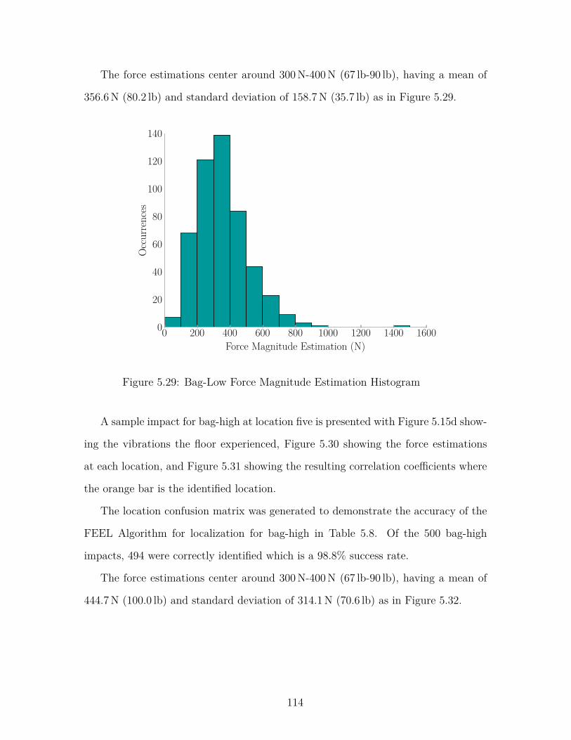
The force estimations center around 300 N-400 N (67 lb-90 lb), having a mean of
356.6 N (80.2 lb) and standard deviation of 158.7 N (35.7 lb) as in Figure 5.29.
0 200 400 600 800 1000 1200 1400 1600Force Magnitude Estimation (N)
0
20
40
60
80
100
120
140O
ccur
renc
es
Figure 5.29: Bag-Low Force Magnitude Estimation Histogram
A sample impact for bag-high at location five is presented with Figure 5.15d show-
ing the vibrations the floor experienced, Figure 5.30 showing the force estimations
at each location, and Figure 5.31 showing the resulting correlation coefficients where
the orange bar is the identified location.
The location confusion matrix was generated to demonstrate the accuracy of the
FEEL Algorithm for localization for bag-high in Table 5.8. Of the 500 bag-high
impacts, 494 were correctly identified which is a 98.8% success rate.
The force estimations center around 300 N-400 N (67 lb-90 lb), having a mean of
444.7 N (100.0 lb) and standard deviation of 314.1 N (70.6 lb) as in Figure 5.32.
114

0.00 0.01 0.02 0.03 0.04Time (s)
−600
−280
40
360
680
1000
Forc
e(N
)Sensor 1Sensor 2Sensor 3Sensor 4
(a) F̂1,j
0.00 0.01 0.02 0.03 0.04Time (s)
−600
−280
40
360
680
1000
Forc
e(N
)
Sensor 1Sensor 2Sensor 3Sensor 4
(b) F̂2,j
0.00 0.01 0.02 0.03 0.04Time (s)
−600
−280
40
360
680
1000
Forc
e(N
)
Sensor 1Sensor 2Sensor 3Sensor 4
(c) F̂3,j
0.00 0.01 0.02 0.03 0.04Time (s)
−600
−280
40
360
680
1000
Forc
e(N
)
Sensor 1Sensor 2Sensor 3Sensor 4
(d) F̂4,j
0.00 0.01 0.02 0.03 0.04Time (s)
−600
−280
40
360
680
1000
Forc
e(N
)
Sensor 1Sensor 2Sensor 3Sensor 4
(e) F̂5,j
Figure 5.30: Bag-High Force Estimations for an Impact on Location 5
115
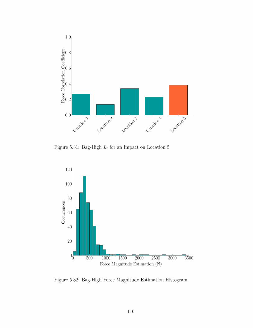
Locat
ion1
Locat
ion2
Locat
ion3
Locat
ion4
Locat
ion5
0.0
0.2
0.4
0.6
0.8
1.0
Forc
eCo
rrela
tion
Coeffi
cient
Figure 5.31: Bag-High Li for an Impact on Location 5
0 500 1000 1500 2000 2500 3000 3500Force Magnitude Estimation (N)
0
20
40
60
80
100
120
Occ
urre
nces
Figure 5.32: Bag-High Force Magnitude Estimation Histogram
116

Table 5.8: Confusion Matrix for Locating Bag-High Impacts
IdentifiedLocation 1 Location 2 Location 3 Location 4 Location 5
Act
ual
Location 1 96 2 1 0 1Location 2 0 100 0 0 0Location 3 0 1 98 0 1Location 4 0 0 0 100 0Location 5 0 0 0 0 100
5.5.4 Human Jump Trials
Three different people jumped at each location 100 times. The trial names indicate
the following: d-jump is a male weighing 80 kg (176 lb), j-jump is a female weighing
55 kg (121 lb), w-jump is a male weighing 85 kg (187 lb). The jump height of each
person varied, and the way the person landed varied as well. This allowed for testing
the FEEL Algorithm and exploring its robustness.
A sample impact for d-jump at location one is presented with Figure 5.15e showing
the vibrations the floor experienced, Figure 5.33 showing the force estimations at
each location, and Figure 5.34 showing the resulting correlation coefficients where
the orange bar is the identified location.
The location confusion matrix was generated to demonstrate the accuracy of the
FEEL Algorithm for localization for the d-jump test in Table 5.9. Of the 500 d-jump
impacts, 476 were correctly identified which is a 95.2% success rate. The algorithm
had the most error at location one where it only had 86% success.
The force estimations center around 700 N-800 N (157 lb-180 lb), having a mean of
711.4 N (159.9 lb) and standard deviation of 226.9 N (51.0 lb) as in Figure 5.35. Since
this trial is record of human-induced vibrations, there is bound to be some variation
as the person jumping would not have jumped to the same height every time. The
spread of estimates is closer together than that of the bag-high trials.
117

0.00 0.06 0.12 0.19 0.25Time (s)
−500
−200
100
400
700
1000
Forc
e(N
)Sensor 1Sensor 2Sensor 3Sensor 4
(a) F̂1,j
0.00 0.06 0.12 0.19 0.25Time (s)
−500
−200
100
400
700
1000
Forc
e(N
)
Sensor 1Sensor 2Sensor 3Sensor 4
(b) F̂2,j
0.00 0.06 0.12 0.19 0.25Time (s)
−500
−200
100
400
700
1000
Forc
e(N
)
Sensor 1Sensor 2Sensor 3Sensor 4
(c) F̂3,j
0.00 0.06 0.12 0.19 0.25Time (s)
−500
−200
100
400
700
1000
Forc
e(N
)
Sensor 1Sensor 2Sensor 3Sensor 4
(d) F̂4,j
0.00 0.06 0.12 0.19 0.25Time (s)
−500
−200
100
400
700
1000
Forc
e(N
)
Sensor 1Sensor 2Sensor 3Sensor 4
(e) F̂5,j
Figure 5.33: D-Jump Force Estimations for an Impact on Location 1
118

Locat
ion1
Locat
ion2
Locat
ion3
Locat
ion4
Locat
ion5
0.0
0.2
0.4
0.6
0.8
1.0
Forc
eCo
rrela
tion
Coeffi
cient
Figure 5.34: D-Jump Li for an Impact on Location 1
0 500 1000 1500 2000 2500Force Magnitude Estimation (N)
0
20
40
60
80
100
120
Occ
urre
nces
Figure 5.35: D-Jump Force Magnitude Estimation Histogram
119
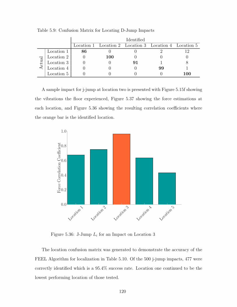
Table 5.9: Confusion Matrix for Locating D-Jump Impacts
IdentifiedLocation 1 Location 2 Location 3 Location 4 Location 5
Act
ual
Location 1 86 0 0 2 12Location 2 0 100 0 0 0Location 3 0 0 91 1 8Location 4 0 0 0 99 1Location 5 0 0 0 0 100
A sample impact for j-jump at location two is presented with Figure 5.15f showing
the vibrations the floor experienced, Figure 5.37 showing the force estimations at
each location, and Figure 5.36 showing the resulting correlation coefficients where
the orange bar is the identified location.
Locat
ion1
Locat
ion2
Locat
ion3
Locat
ion4
Locat
ion5
0.0
0.2
0.4
0.6
0.8
1.0
Forc
eCo
rrela
tion
Coeffi
cient
Figure 5.36: J-Jump Li for an Impact on Location 3
The location confusion matrix was generated to demonstrate the accuracy of the
FEEL Algorithm for localization in Table 5.10. Of the 500 j-jump impacts, 477 were
correctly identified which is a 95.4% success rate. Location one continued to be the
lowest performing location of those tested.
120

0.00 0.06 0.12 0.19 0.25Time (s)
−400
−160
80
320
560
800
Forc
e(N
)Sensor 1Sensor 2Sensor 3Sensor 4
(a) F̂1,j
0.00 0.06 0.12 0.19 0.25Time (s)
−400
−160
80
320
560
800
Forc
e(N
)
Sensor 1Sensor 2Sensor 3Sensor 4
(b) F̂2,j
0.00 0.06 0.12 0.19 0.25Time (s)
−400
−160
80
320
560
800
Forc
e(N
)
Sensor 1Sensor 2Sensor 3Sensor 4
(c) F̂3,j
0.00 0.06 0.12 0.19 0.25Time (s)
−400
−160
80
320
560
800
Forc
e(N
)
Sensor 1Sensor 2Sensor 3Sensor 4
(d) F̂4,j
0.00 0.06 0.12 0.19 0.25Time (s)
−400
−160
80
320
560
800
Forc
e(N
)
Sensor 1Sensor 2Sensor 3Sensor 4
(e) F̂5,j
Figure 5.37: J-Jump Force Estimations for an Impact on Location 3
121
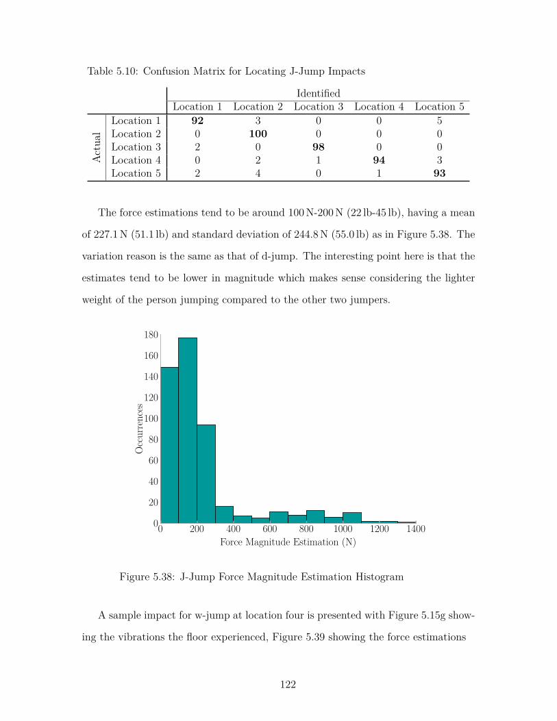
Table 5.10: Confusion Matrix for Locating J-Jump Impacts
IdentifiedLocation 1 Location 2 Location 3 Location 4 Location 5
Act
ual
Location 1 92 3 0 0 5Location 2 0 100 0 0 0Location 3 2 0 98 0 0Location 4 0 2 1 94 3Location 5 2 4 0 1 93
The force estimations tend to be around 100 N-200 N (22 lb-45 lb), having a mean
of 227.1 N (51.1 lb) and standard deviation of 244.8 N (55.0 lb) as in Figure 5.38. The
variation reason is the same as that of d-jump. The interesting point here is that the
estimates tend to be lower in magnitude which makes sense considering the lighter
weight of the person jumping compared to the other two jumpers.
0 200 400 600 800 1000 1200 1400Force Magnitude Estimation (N)
0
20
40
60
80
100
120
140
160
180
Occ
urre
nces
Figure 5.38: J-Jump Force Magnitude Estimation Histogram
A sample impact for w-jump at location four is presented with Figure 5.15g show-
ing the vibrations the floor experienced, Figure 5.39 showing the force estimations
122
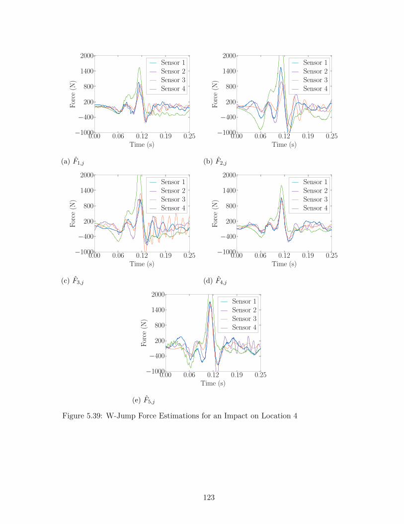
0.00 0.06 0.12 0.19 0.25Time (s)
−1000
−400
200
800
1400
2000
Forc
e(N
)Sensor 1Sensor 2Sensor 3Sensor 4
(a) F̂1,j
0.00 0.06 0.12 0.19 0.25Time (s)
−1000
−400
200
800
1400
2000
Forc
e(N
)
Sensor 1Sensor 2Sensor 3Sensor 4
(b) F̂2,j
0.00 0.06 0.12 0.19 0.25Time (s)
−1000
−400
200
800
1400
2000
Forc
e(N
)
Sensor 1Sensor 2Sensor 3Sensor 4
(c) F̂3,j
0.00 0.06 0.12 0.19 0.25Time (s)
−1000
−400
200
800
1400
2000
Forc
e(N
)
Sensor 1Sensor 2Sensor 3Sensor 4
(d) F̂4,j
0.00 0.06 0.12 0.19 0.25Time (s)
−1000
−400
200
800
1400
2000
Forc
e(N
)
Sensor 1Sensor 2Sensor 3Sensor 4
(e) F̂5,j
Figure 5.39: W-Jump Force Estimations for an Impact on Location 4
123
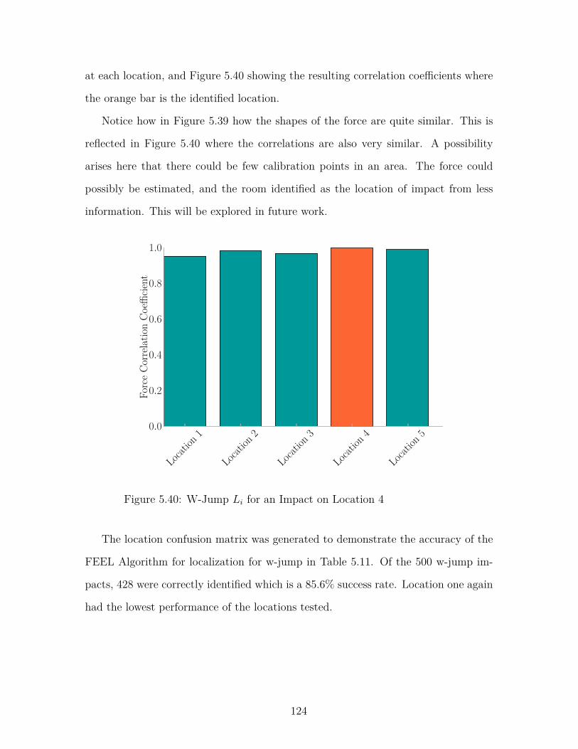
at each location, and Figure 5.40 showing the resulting correlation coefficients where
the orange bar is the identified location.
Notice how in Figure 5.39 how the shapes of the force are quite similar. This is
reflected in Figure 5.40 where the correlations are also very similar. A possibility
arises here that there could be few calibration points in an area. The force could
possibly be estimated, and the room identified as the location of impact from less
information. This will be explored in future work.
Locat
ion1
Locat
ion2
Locat
ion3
Locat
ion4
Locat
ion5
0.0
0.2
0.4
0.6
0.8
1.0
Forc
eCo
rrela
tion
Coeffi
cient
Figure 5.40: W-Jump Li for an Impact on Location 4
The location confusion matrix was generated to demonstrate the accuracy of the
FEEL Algorithm for localization for w-jump in Table 5.11. Of the 500 w-jump im-
pacts, 428 were correctly identified which is a 85.6% success rate. Location one again
had the lowest performance of the locations tested.
124

Table 5.11: Confusion Matrix for Locating W-Jump Impacts
IdentifiedLocation 1 Location 2 Location 3 Location 4 Location 5
Act
ual
Location 1 45 6 4 13 32Location 2 1 98 0 0 1Location 3 3 3 90 0 4Location 4 0 0 1 96 3Location 5 0 1 0 0 99
The force estimations center around 900 N-1000 N (202 lb-225 lb), having a mean
of 947.1 N (212.9 lb) and standard deviation of 421.5 N (97.8 lb) as in Figure 5.41. The
variation in magnitudes is due to the same reason as that of d-jump and j-jump trials.
This test had the heaviest person jumping which the histogram demonstrates with
the majority of jumps being higher in magnitude than the other two participants.
0 500 1000 1500 2000 2500Force Magnitude Estimation (N)
0
10
20
30
40
50
60
Occ
urre
nces
Figure 5.41: W-Jump Force Estimation Histogram
125

5.6 Implementation Experiment Resampled
The following describes the effect of resampling on the performance of FEEL.
5.6.1 Using Sampling Frequency of 400 Hz
The data collected during the experiment presented in Section 5.5, was downsam-
pled to 400 Hz using the Fourier Method [21, 45]. This would determine if the higher
frequencies present in the data affect the force estimate and event localization. The
results presented below point towards the new rate being more effective than the orig-
inal sampling rate. It is then verified that the FEEL Algorithm can be implemented
at a relatively low sampling frequency to reduce computational cost.
The experiment first started with the force estimate difference for the hammer
impacts as a signifier of force magnitude estimation accuracy shown in Figure 5.42.
With the new sampling frequency of 400 Hz, the differences became much smaller
having a mean of 109.9 N (24.7 lb) and standard deviation of 99.1 N (22.3 lb). The
accuracy improved placing 85.3% of force differences within the 200 N (45 lb) range,
an increase of 13.3% from the original estimates presented in Figure 5.19. The 99%
confidence interval for force magnitude estimation error also improved becoming -1.7%
± 1.0% based on Figure 5.43 where the mean is -1.7% and the standard deviation is
3.5%.
The next measure was event localization accuracy which is displayed in a confusion
matrix of Table 5.12. Originally across all action types, there were 3447 correctly
located out of 3575 records for a 96.4% overall accuracy rate. Resampling brought the
location accuracy down to 90.7% correct, or 3244 out of 3575. The event localization
accuracy still remains very high showing that the FEEL Algorithm can be used for
localization at lower sampling rates.
The results indicate that as one lowers the sampling rate, the location accuracy
decreases, while the force magnitude estimation accuracy increases. Sampling rate
126

0 100 200 300 400 500Force Magnitude Difference (N)
0
5
10
15
20
25
30
35
40
45
Occ
urre
nces
Figure 5.42: Force Magnitude Estimation Difference for ConcreteFloor Impacts Using Data Downsampled to 400 Hz
−15 −10 −5 0 5 10Force Magnitude Error (%)
0
5
10
15
20
25
Occ
urre
nces
Figure 5.43: Force Magnitude Estimation Error for Concrete FloorImpacts Using Data Downsampled to 400 Hz
127
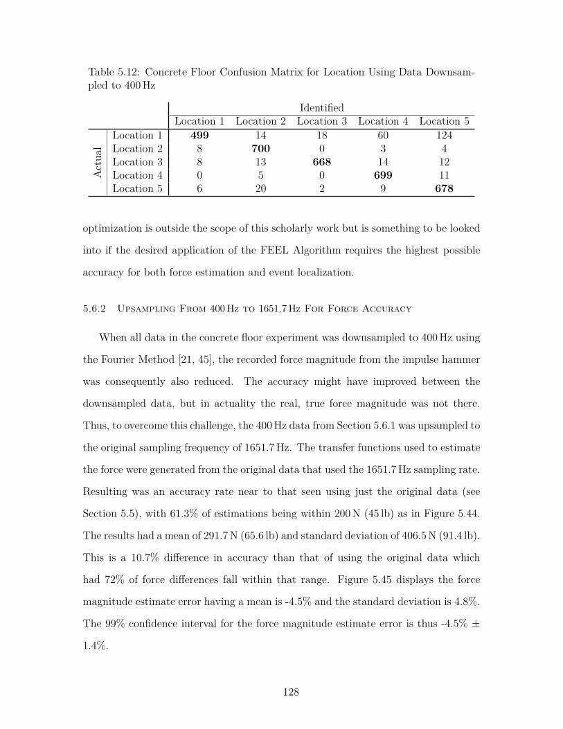
Table 5.12: Concrete Floor Confusion Matrix for Location Using Data Downsam-pled to 400 Hz
IdentifiedLocation 1 Location 2 Location 3 Location 4 Location 5
Act
ual
Location 1 499 14 18 60 124Location 2 8 700 0 3 4Location 3 8 13 668 14 12Location 4 0 5 0 699 11Location 5 6 20 2 9 678
optimization is outside the scope of this scholarly work but is something to be looked
into if the desired application of the FEEL Algorithm requires the highest possible
accuracy for both force estimation and event localization.
5.6.2 Upsampling From 400 Hz to 1651.7 Hz For Force Accuracy
When all data in the concrete floor experiment was downsampled to 400 Hz using
the Fourier Method [21, 45], the recorded force magnitude from the impulse hammer
was consequently also reduced. The accuracy might have improved between the
downsampled data, but in actuality the real, true force magnitude was not there.
Thus, to overcome this challenge, the 400 Hz data from Section 5.6.1 was upsampled to
the original sampling frequency of 1651.7 Hz. The transfer functions used to estimate
the force were generated from the original data that used the 1651.7 Hz sampling rate.
Resulting was an accuracy rate near to that seen using just the original data (see
Section 5.5), with 61.3% of estimations being within 200 N (45 lb) as in Figure 5.44.
The results had a mean of 291.7 N (65.6 lb) and standard deviation of 406.5 N (91.4 lb).
This is a 10.7% difference in accuracy than that of using the original data which
had 72% of force differences fall within that range. Figure 5.45 displays the force
magnitude estimate error having a mean is -4.5% and the standard deviation is 4.8%.
The 99% confidence interval for the force magnitude estimate error is thus -4.5% ±
1.4%.
128

0 500 1000 1500 2000 2500 3000Force Magnitude Difference (N)
0
5
10
15
20
25
Occ
urre
nces
Figure 5.44: Force Magnitude Estimation for Concrete Floor ImpactsUsing Data Upsampled From 400 Hz to 1651.7 Hz
−25 −20 −15 −10 −5 0 5Force Magnitude Error (%)
0
5
10
15
20
25
30
Occ
urre
nces
Figure 5.45: orce Magnitude Estimation Error for Concrete FloorImpacts Using Data Upsampled From 400 Hz to 1651.7 Hz
129
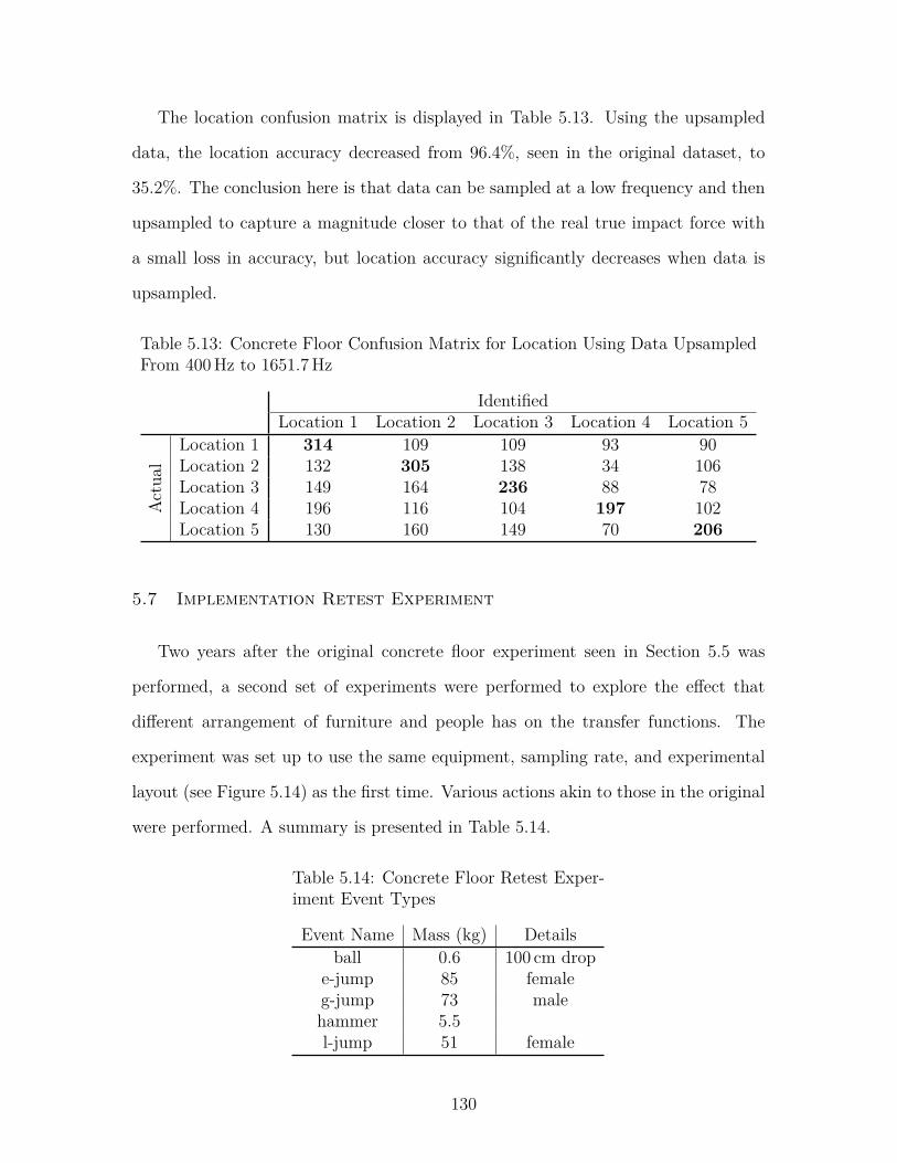
The location confusion matrix is displayed in Table 5.13. Using the upsampled
data, the location accuracy decreased from 96.4%, seen in the original dataset, to
35.2%. The conclusion here is that data can be sampled at a low frequency and then
upsampled to capture a magnitude closer to that of the real true impact force with
a small loss in accuracy, but location accuracy significantly decreases when data is
upsampled.
Table 5.13: Concrete Floor Confusion Matrix for Location Using Data UpsampledFrom 400 Hz to 1651.7 Hz
IdentifiedLocation 1 Location 2 Location 3 Location 4 Location 5
Act
ual
Location 1 314 109 109 93 90Location 2 132 305 138 34 106Location 3 149 164 236 88 78Location 4 196 116 104 197 102Location 5 130 160 149 70 206
5.7 Implementation Retest Experiment
Two years after the original concrete floor experiment seen in Section 5.5 was
performed, a second set of experiments were performed to explore the effect that
different arrangement of furniture and people has on the transfer functions. The
experiment was set up to use the same equipment, sampling rate, and experimental
layout (see Figure 5.14) as the first time. Various actions akin to those in the original
were performed. A summary is presented in Table 5.14.
Table 5.14: Concrete Floor Retest Exper-iment Event Types
Event Name Mass (kg) Detailsball 0.6 100 cm drop
e-jump 85 femaleg-jump 73 malehammer 5.5l-jump 51 female
130

0.0 0.2 0.4 0.6 0.8 1.0Time (s)
−0.15
−0.10
−0.05
0.00
0.05
0.10
0.15
Acce
lerat
ion
(g)
Sensor 1Sensor 2Sensor 3Sensor 4
(a) Ball
0.0 0.2 0.4 0.6 0.8 1.0Time (s)
−0.15
−0.10
−0.05
0.00
0.05
0.10
0.15
Acce
lerat
ion
(g)
Sensor 1Sensor 2Sensor 3Sensor 4
(b) E-Jump
0.0 0.2 0.4 0.6 0.8 1.0Time (s)
−0.15
−0.10
−0.05
0.00
0.05
0.10
0.15
Acce
lerat
ion
(g)
Sensor 1Sensor 2Sensor 3Sensor 4
(c) G-Jump
0.0 0.2 0.4 0.6 0.8 1.0Time (s)
−0.15
−0.10
−0.05
0.00
0.05
0.10
0.15
Acce
lerat
ion
(g)
Sensor 1Sensor 2Sensor 3Sensor 4
(d) L-Jump
0.0 0.2 0.4 0.6 0.8 1.0Time (s)
−1.5
−1.0
−0.5
0.0
0.5
1.0
1.5
Acce
lerat
ion
(g)
Sensor 1Sensor 2Sensor 3Sensor 4
(e) Hammer
Figure 5.46: Concrete Floor Retest Experiment Example Accelerations
131

Each event type had five repetitions performed at five different locations for a
total of 25 records per event, and giving 125 available records in total. Figure 5.46
gives example accelerations for each event type.
The transfer functions from the original dataset (Section 5.5) were applied to
the 125 records of the retest dataset. Table 5.15 provides the confusion matrix for
location identification, with the shaded regions indicating local areas. The ability to
identify location dropped from average 96.8% correct to 70.4% with locations four
and five showing the most change. With large redistribution of the loading in the
room, the transfer functions have thus changed significantly at locations 4 and 5.
Local area identification demonstrates 80% accuracy and indicates a good ability to
perform regional localization in the face of significant change in loading.
Table 5.15: Implementation Retest Confusion Matrix for Location
IdentifiedLocation 1 Location 2 Location 3 Location 4 Location 5
Act
ual
Location 1 20 1 1 1 2Location 2 0 25 0 0 0Location 3 0 6 19 0 0Location 4 1 1 1 11 11Location 5 5 0 7 0 13
Force magnitude estimation is compared to the measured hammer force in Fig-
ure 5.47. The differences had a mean of 1533.1 N (344.7 lb) and a standard deviation
of 1736.7 N (390.4 lb), indicating FEEL was having difficulty in estimating force of
impact under the new loading conditions. This is further backed by Figure 5.48 which
gives the 99% confidence interval for force magnitude estimation error as 16.2% ±
8.4%. In conclusion, the transfer functions should be re-calibrated when significant
furniture rearrangement is done.
132

0 1000 2000 3000 4000 5000Force Magnitude Difference (N)
0
1
2
3
4
5
Occ
urre
nces
Figure 5.47: Difference Between Force Magnitude Estimation AndMeasured Hammer Force for Implementation Retest Experiment
−80 −60 −40 −20 0 20 40 60 80 100Force Error (%)
0
1
2
3
4
5
6
7
8
9
Occ
urre
nces
Figure 5.48: Error Between Force Magnitude Estimation And Mea-sured Hammer Force for Implementation Retest Experiment
133
5.8 Conclusion
Most of the challenges faced by current detection systems based in structural vi-
brations are overcome through the application of the Force Estimation and Event
Localization (FEEL) Algorithm. Structural vibrations, which naturally contain the
dynamic attributes of the structure, are directly related to the impact force and loca-
tion. Challenges arising from structural property variation are thus eliminated, and
challenges of distance between a sensor and an event are overcome. Time synchro-
nization is not required for applying FEEL, making implementation easier than other
methods.
The algorithm exhibits great performance with 96.4% average accuracy in recog-
nizing impact location in over 3575 impacts of eight different types, and having a
force magnitude estimation error of -2.0% ± 1.3% for the 99% confidence interval. A
brief look how FEEL works at a lower sampling rate, 400 Hz in this case, indicates
that location accuracy decreases and force magnitude estimation accuracy increases
when compared to a higher sampling rate of 1651.7 Hz. However, the force actually
experienced by the structure is larger than what the signal captured at the lower
sampling rate sees. Data can be captured at a low sampling rate and upsampled
to close the gap between the force magnitude estimation and the force experienced
by the structure to alleviate this problem. Upsampling, however, does not increase
localization accuracy, but instead decreases it. In addition for long term implementa-
tions, there is a need to re-calibrate the transfer functions when significant furniture
rearranging in an area is done to maintain FEEL’s high accuracy.
134

Chapter 6
EFFECT Active Learning Module For The
Frequency Domain
6.1 Introduction
Traditionally research dissertations focus on reporting a contribution to a spe-
cific area. However, the job of an academician goes beyond the discovery of new
knowledge to disseminating that knowledge through education. Dr. Juan M. Caicedo
encourages doctoral students that are interested in academia to apply to programs
such as the Preparing Future Faculty program and explore other aspects of the aca-
demic life such as teaching and service [47]. He also encourages students to explore
the use of effective teaching techniques by including a chapter in their dissertation
focusing in education rather than research. This chapter should not be an island of
the dissertation, and the topics should be relevant to those covered in the rest of the
work. This chapter discusses the use of active learning, “defined as any instructional
method that engages students in the learning process” [48], to teach concepts that
are difficult to conceptualize in structural dynamics. These concepts are particularly
important to understand the rest of the work presented herein.
Material such as that provided within this work can be difficult to grasp for stu-
dents without prior knowledge in dynamics due to the complexity of many of the
basic concepts. The Environments For Fostering Effective Critical Thinking (EF-
FECT) framework is used here to engage critical thinking skills and improve the
transfer of knowledge [49, 50, 51]. EFFECT was originally created in 2008 with a
135

focus on freshmen engineering students to increase retention and improve outcomes
in the aforementioned areas and has since seen expansion to other college levels [49,
52, 53, 54]. Accreditation Board for Engineering and Technology (ABET) and Amer-
ican Society of Civil Engineers (ASCE) student outcomes can be addressed by each
full EFFECT making it a natural choice for engineering education, particularly in
the realms of communication skills, teamwork, and knowledge of contemporary is-
sues [53]. The EFFECT developmental framework provides a procedure that guides
instructors in creation of an EFFECT. The framework, in summary, follows this pro-
cedure: (1) critical concepts should be identified, (2) active learning modules are
developed for those concepts, (3) context provided for the EFFECT, and (4) a driv-
ing question and supporting question for a decision worksheet are developed [55]. It
is highly recommended that instructors test and perfect the active learning modules
before continuing with providing a context and designing a decision worksheet.
In this work, only the first two steps are completed. The outcome is an active
learning module for the concept of frequency domain representation of signals, a
concept heavily used in the FEEL Algorithm seen in Chapter 5. The module pro-
vides a foundation on which to expand into a full EFFECT for areas that work
with frequency domain based analysis, and will be provided on the EFFECT website
(https://sdii.ce.sc.edu/effects/).
6.2 The EFFECT Pedagogical Framework
EFFECT’s pedagogical framework, presented in Figure 6.1, “links the two critical
elements of active learning and reflective writing” [51] to stimulate the learner to
think critically about a topic presented [49, 51] and is what students experience in
class. An EFFECT begins with a decision worksheet where students thoughts are
framed in a design problem individually and then in concert with a group. The groups
discuss their varying opinions and provide support for their arguments. Everyone has
136
a different knowledge set, thus this encourages students to think through each others’
ideas which in itself requires critical thinking or meta-cognition of what factors they
do not know. Driving questions are then supported by any number of interchangeable
active learning modules designed to give hands on experience to explore topics. The
modules can challenge students’ preconceived notions which may vary well be mis-
conceptions, encouraging self-discovery of knowledge. After each module, students
submit journal entries about class activities addressing the hows and whys the new
material can aid them in the design problem. This further directs students to think
deeply about a concept. The end of an EFFECT is a group and class discussion
about everything that was learned to come up with their new answers to the driving
question after they have corrected any misconceptions and expanded their knowledge
base. Afterwards, students submit final reports with their designs [49, 50, 51].
6.3 The EFFECT Developmental Framework
The developmental framework, outlined in Figure 6.2, takes a “think big, start
small” approach to creating a full EFFECT [55]. Individual elements of an EFFECT
are implemented first, and then refined in an iterative process based on feedback from
students and teacher evaluations of both self and the class. Items like how well did
the activity work in getting the understanding across or was the activity engaging
enough to encourage students to use critical thinking are of particular interest. Over
time, all the individual components of an EFFECT are combined to create the full
EFFECT and are linked together through a decision worksheet which has a context
and a set of driving and guiding questions to direct students on the learning process
[55].
The first step to creating a full EFFECT begins by the instructor identifying
concepts to be taught. Following this, active learning modules are created to demon-
strate the concepts through hands-on experiences, jigsaw class, or other engaging
137

DecisionWorksheet
ActiveLearningModule 1
ActiveLearningModule 2
ActiveLearningModule n
Redesign& Group
Discussion
Final Design& Report
Journal Entry
Journal Entry
Journal Entry
Journal Entry
Figure 6.1: EFFECT PedagogicalStructure [49, 50, 51]
active learning techniques [56, 57, 58, 59, 60, 61, 62, 63]. These two steps are done
iteratively for several classes to improve upon the active learning modules so that
knowledge transfer is maximized and critical thinking is engaged. The third step is
to connect the concepts to a real world application. This aids in deep learning as
students link what they are seeing to something they are more familiar with or is
138
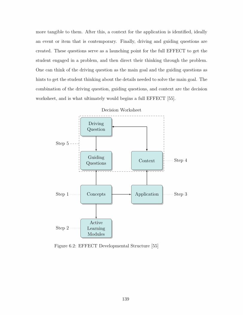
more tangible to them. After this, a context for the application is identified, ideally
an event or item that is contemporary. Finally, driving and guiding questions are
created. These questions serve as a launching point for the full EFFECT to get the
student engaged in a problem, and then direct their thinking through the problem.
One can think of the driving question as the main goal and the guiding questions as
hints to get the student thinking about the details needed to solve the main goal. The
combination of the driving question, guiding questions, and context are the decision
worksheet, and is what ultimately would begins a full EFFECT [55].
DrivingQuestion
GuidingQuestions
Concepts
ActiveLearningModules
Application
Context
Decision Worksheet
Step 1
Step 2
Step 3
Step 4
Step 5
Figure 6.2: EFFECT Developmental Structure [55]
139
6.4 Concept Selection
Meetings with Dr. Juan M. Caicedo were spent discussing topics explored in this
work to select concepts that were, based on his instruction experience, difficult for
students to grasp. The concept of frequency domain representation of signals, some-
thing used heavily in the FEEL Algorithm, was identified as a difficult concept for
students and is the subject of the active learning module presented in Section 6.5 [47].
Frequency domain is not as utilized or explored in basic structural dynamics classes
as time domain is, and students typically think in terms of time instead of excitation
frequency to the overall signal. Hence, the selected topic was chosen as the subject
of an active learning module so that students can learn the concept effectively.
6.5 Active Learning Module
As a step towards creating a full EFFECT, the following active learning mod-
ule was created based on the format provided from the EFFECT website [54]. The
module focuses on the use of a steel frame test structure at the University of South
Carolina (USC) seen in Section 5.4; however, any structure can be used provided
that it has more visible responses to loading (e.g. large displacements) and one knows
or can estimate the first natural frequency. This ensures the students can both feel
and see what is happening with the structure. The module additionally provides the
opportunity for students to improve communication and teamwork skills through a
jigsaw-styled class where some students become ‘experts’ in the mathematical for-
mulas and others in the physical results, enabling the students to teach one another.
This method places emphasis on cooperation as the student group is less likely to
succeed without everyone coming together as a team, thus encouraging everyone’s
engagement with the subject matter [62]. Due to the potential demands of the expe-
rience, this module is designed for pairs of ‘experts’ so that students can share the
140

demands for each piece. Students are additionally encouraged to take notes in the
focus groups to additionally ease the social demand [57].
Concept Frequency domain representation of signals
Audience College Junior/Senior
Estimated Time 75 minutes
Materials
1. Steel frame (or other structure). See Section 5.4.
2. DAQ. Used NI 9234 Module.
3. Accelerometer. Used PCB 333B50.
4. Computer (to operate DAQ).
5. Hammer (for impulse excitation). Used PCB 086C03.
6. Graph paper.
Description Begin by splitting class into two halves. One half will remain in
the classroom where an instructor will introduce the concept using typical classroom
instruction. The other half will proceed to the location of the steel frame for a hands
on explanation of the concept.
Classroom: Explain what is frequency domain is, and how it differs from the time
domain we often see. Talk about how any signal can be broken down into multiple
sines and cosines having their own frequency and amplitude. In other words, multiple
waveforms combine together to form a signal much like multiple instruments make
up an orchestra, and one hears all the instruments together or can focus in on one
particular instrument, i.e. a specific waveform within the greater signal. Talk about
the math for converting a time domain signal into frequency domain through the
141

Fourier Transform. A handout to aid with instruction on the topic is provided in
Appendix J.
Laboratory: Start by explaining what frequency domain is, and how it differs from
the time domain we often see. Talk about how any signal can be broken down into
multiple waveforms having their own frequency. Have the students plot their predic-
tion of what a 1 Hz harmonic loading would look like in the frequency domain. Then
ask the students to push the frame at an approximate rate of 1 Hz, recording the ac-
celerations. Using software such as Signal Express, convert the recorded time domain
data into frequency domain and plot for the students to see. Prompt them to talk
about the differences between their predictions and the result from the experiment.
Repeat the prediction and experiment for two other excitation frequencies: 5 Hz and
10 Hz.
If using a different structure than the steel frame, choose three rates where one
is less than the first natural frequency, one about the first natural frequency, and
finally, one after the first natural frequency. This will give the same outcome as the
steel frame.
Combined Groups: After each respective group (classroom and laboratory) is
done, bring the laboratory group back to the classroom. Take groups of four with
two from the initial classroom group and two from the initial laboratory group. Have
the student groups relate the classroom instruction to the instruction the laboratory
students had. Have the students come up with an idea of what is happening in various
parts of the graph. Students will then present what they have learned to the class,
with the instructors prompting for other groups who have different explanations.
The groups will then be asked to come up with an estimate of what would happen
if the steel frame came under simultaneous loadings, one loading at each of the rates
used previously (1 Hz, 5 Hz, 10 Hz). Then ask them what they would expect a hammer
hit would look like in the frequency domain. Each group should generate a new set
142

of response vs. frequency plots for the two cases. Instructor prompts for groups to
describe their plots and reasoning for their expected results.
Take the whole class back to the laboratory with the steel frame. Have three
different students apply a loading at the three rates simultaneously. On Signal Ex-
press, the frequency representation of the signal can be updated in real time so that
the students may compare their estimates to reality. Ask them about the differences
between what they thought and what the results are showing. Why do the results
look that way?
Repeat the experiment using the hammer to excite the structure. Plot the fre-
quency domain representation of the signal. Ask the students about the differences
between what they thought and what the results are showing. Why do the results
look that way? What do the peaks in the frequency domain mean? Discuss what the
students observed and how/why their thinking differs from reality.
Expected Outcomes The expected outcomes include students learning about
that signals can be represented in different domains, the frequency domain in partic-
ular. Students are expected to begin to understand a relationship between structural
response in the time domain and power in the frequency domain, and that one signal
can be broken into multiple sinusoidals that have their own frequencies. The concept
of superposition can be reinforced with discussions on why multiple signals can be
combined into one as well.
Students are expected to begin answering questions about the frequency domain
as if it is the time domain. After a few experiments and discuss, students then are ex-
pected to realize the frequency domain operates differently than the time domain and
be able to correctly predict what the signal representation in the frequency domain
looks like.
143
6.6 Conclusion
The active learning module was used in a structural vibrations engineering class
at USC having fifteen students. In the class period after the module, an anonymous
survey (see Appendix K) was administered to gain feedback from students on how to
improve the module and nine students responded. Survey responses are provided in
Appendix L, and a summary of scores is provided in Table 6.1 where a score of one
is not conducive/confident and a score of five is conducive/confident.
A post-class interview with the instructor indicated that the scores presented in
Table 6.1 were representative of exam performance in each topic [64]. Confidence
scores for Single Degree of Freedom (SDOF) Periodic Excitation and Frequency Do-
main Signal Representation confirms that they are topics that are challenging for
students, i.e. they perceive the topics as being challenging, as thought by the instruc-
tor. Surveys were not taken in prior years, so a similar survey needs to be done in
subsequent years (longitudinal study) to see if student mean confidence increases.
The breakdown of scores by students’ expected grades are displayed in Figure 6.3.
All students regardless of expected grade thought the class lectures were all very
conducive to their learning. In-class homeworks were not regarded as conducive with
a student commenting on how he felt the format was more like a quiz than a homework
with the instructor not providing much aid. The project was considered conducive,
however, some students wanted more guidance or instruction before tackling the
assignment.
Experiments and lab visits were regarded as conducive, with student responses to
Question 6 (Did the lab visit make the connection between math and physics easier to
understand? How or why?) reinforcing scores in Question 3 (Indicate how conducive
to learning the following course activities were.). Figure 6.4 displays the breakdown of
responses for Question 6.a where students were asked if the lab visit allowed them to
144
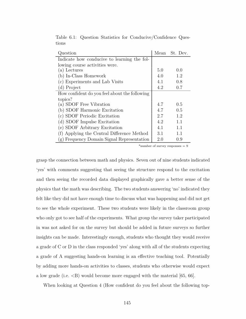
Table 6.1: Question Statistics for Conducive/Confidence Ques-tions
Question Mean St. Dev.Indicate how conducive to learning the fol-lowing course activities were.(a) Lectures 5.0 0.0(b) In-Class Homework 4.0 1.2(c) Experiments and Lab Visits 4.1 0.8(d) Project 4.2 0.7How confident do you feel about the followingtopics?(a) SDOF Free Vibration 4.7 0.5(b) SDOF Harmonic Excitation 4.7 0.5(c) SDOF Periodic Excitation 2.7 1.2(d) SDOF Impulse Excitation 4.2 1.1(e) SDOF Arbitrary Excitation 4.1 1.1(f) Applying the Central Difference Method 3.1 1.1(g) Frequency Domain Signal Representation 2.0 0.9
*number of survey responses = 9
grasp the connection between math and physics. Seven out of nine students indicated
‘yes’ with comments suggesting that seeing the structure respond to the excitation
and then seeing the recorded data displayed graphically gave a better sense of the
physics that the math was describing. The two students answering ‘no’ indicated they
felt like they did not have enough time to discuss what was happening and did not get
to see the whole experiment. These two students were likely in the classroom group
who only got to see half of the experiments. What group the survey taker participated
in was not asked for on the survey but should be added in future surveys so further
insights can be made. Interestingly enough, students who thought they would receive
a grade of C or D in the class responded ‘yes’ along with all of the students expecting
a grade of A suggesting hands-on learning is an effective teaching tool. Potentially
by adding more hands-on activities to classes, students who otherwise would expect
a low grade (i.e. <B) would become more engaged with the material [65, 66].
When looking at Question 4 (How confident do you feel about the following top-
145

1 2 3 4 5Score
0
2
4
6
8
10
Coun
t
ABCD
(a) Lectures
1 2 3 4 5Score
0
2
4
6
8
10
Coun
t
ABCD
(b) In-Class Homework
1 2 3 4 5Score
0
2
4
6
8
10
Coun
t
ABCD
(c) Experiments and Lab Visits
1 2 3 4 5Score
0
2
4
6
8
10
Coun
t
ABCD
(d) Project
Figure 6.3: Distribution of Responses Broken Down by Students’ Ex-pected Grade for Question 3 “Indicate How Conducive to Learning TheFollowing Course Activities Were”
ics.) which served to indicate how confident students felt on their grasp of concepts
presented in the class, there were mixed results as seen in Figure 6.5. Free vibration
and harmonic excitation are topics the students felt confident about, and are also
topics taught at the beginning of the semester. Periodic and impulse excitation are
more complex topics, with the students reporting varying levels of confidence levels.
Students reported having more confidence with arbitrary excitation even though this
topic is ‘an extension’ of impulse excitation. The central difference method had an
mean score of 3.1 showing students had a moderate confidence level about the topic.
Of particular interest to the author is the scores for the frequency domain represen-
tation which was only taught through the active learning module for a single class
period. Students reported not being very confident (score ≤ 3) which suggests some
146
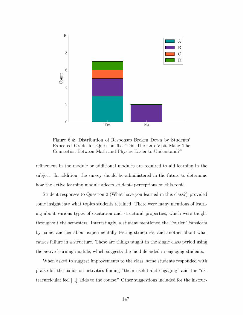
Yes No0
2
4
6
8
10
Coun
t
ABCD
Figure 6.4: Distribution of Responses Broken Down by Students’Expected Grade for Question 6.a “Did The Lab Visit Make TheConnection Between Math and Physics Easier to Understand?”
refinement in the module or additional modules are required to aid learning in the
subject. In addition, the survey should be administered in the future to determine
how the active learning module affects students perceptions on this topic.
Student responses to Question 2 (What have you learned in this class?) provided
some insight into what topics students retained. There were many mentions of learn-
ing about various types of excitation and structural properties, which were taught
throughout the semesters. Interestingly, a student mentioned the Fourier Transform
by name, another about experimentally testing structures, and another about what
causes failure in a structure. These are things taught in the single class period using
the active learning module, which suggests the module aided in engaging students.
When asked to suggest improvements to the class, some students responded with
praise for the hands-on activities finding “them useful and engaging” and the “ex-
tracurricular feel [...] adds to the course.” Other suggestions included for the instruc-
147

tor to give an overview of concepts to be thinking about during the experiments or to
have more class discussion in addition to the ‘expert’ groups. A few responses asked
for more time to work with the material and to get to see all of the experiments. This
thought is further backed by instructors’ observation that the classroom group of stu-
dents asked more questions to gain understanding of the base concepts whereas the
experiment group was able to piece the concepts together and ask more application
1 2 3 4 5Score
0
2
4
6
8
10
Coun
t
ABCD
(a) SDOF Free Vibration
1 2 3 4 5Score
0
2
4
6
8
10
Coun
t
ABCD
(b) SDOF Harmonic Excitation
1 2 3 4 5Score
0
2
4
6
8
10
Coun
t
ABCD
(c) SDOF Periodic Excitation
1 2 3 4 5Score
0
2
4
6
8
10
Coun
t
ABCD
(d) SDOF Impulse Excitation
1 2 3 4 5Score
0
2
4
6
8
10
Coun
t
ABCD
(e) SDOF Arbitrary Excitation
1 2 3 4 5Score
0
2
4
6
8
10
Coun
t
ABCD
(f) Applying the Central DifferenceMethod
148
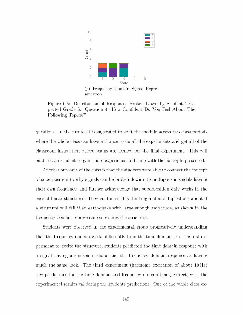
1 2 3 4 5Score
0
2
4
6
8
10
Coun
t
ABCD
(g) Frequency Domain Signal Repre-sentation
Figure 6.5: Distribution of Responses Broken Down by Students’ Ex-pected Grade for Question 4 “How Confident Do You Feel About TheFollowing Topics?”
questions. In the future, it is suggested to split the module across two class periods
where the whole class can have a chance to do all the experiments and get all of the
classroom instruction before teams are formed for the final experiment. This will
enable each student to gain more experience and time with the concepts presented.
Another outcome of the class is that the students were able to connect the concept
of superposition to why signals can be broken down into multiple sinusoidals having
their own frequency, and further acknowledge that superposition only works in the
case of linear structures. They continued this thinking and asked questions about if
a structure will fail if an earthquake with large enough amplitude, as shown in the
frequency domain representation, excites the structure.
Students were observed in the experimental group progressively understanding
that the frequency domain works differently from the time domain. For the first ex-
periment to excite the structure, students predicted the time domain response with
a signal having a sinusoidal shape and the frequency domain response as having
much the same look. The third experiment (harmonic excitation of about 10 Hz)
saw predictions for the time domain and frequency domain being correct, with the
experimental results validating the students predictions. One of the whole class ex-
149

periments was not performed due to time constraints, but the impulse experiment
saw students connecting how an impulse excites the natural frequencies of a structure
and further seeing students realize a structure has many natural frequencies, not just
one.
Overall, the active learning module appears to have encouraged students’ critical
thinking and engagement. Future iterations to better refine the module are suggested
to (1) expand the module over two class periods, (2) to allow the entire class to cycle
through the experiments, and (3) provide ample time for discussion and demonstra-
tions during classroom instruction.
150

Chapter 7
Conclusion
Wireless smart accelerometers were implemented in system boasting a star net-
work topology which allowed for each sensor to operate independently to dynamically
adjust to their respective local environment. The sensors themselves, had a success
rate of 62% in capturing the falls reported by the study participants. Falls missed
by the sensors were likely due to low-force impacts that would not have resulted in
severe injury. The remaining fall events missed were due to several failures modes,
the most predominant of which being the power supply to the sensors being mistaken
for a phone charger. Together, the accelerometers experienced a wear out failure
trend with a 5.06 × 10⁻³ failureshour failure rate and a 197.7 hours Mean Time Between
Failure (MTBF). This equates to a 4.9% chance to capture a human fall in a year. A
successful system would instead need a 99% chance to capture a fall, which means a
MTBF of 8642.4 hours is required for the sensors.
Other characteristic recommendations for the wireless accelerometers emerged
when working with the vibration monitoring system. The 16 human fall events cap-
tured by the system indicate a buffer size of 3 s suggested by Yu is sufficient to capture
the full waveform, and important aspect when dealing with limited resources of an
embedded sensor [6]. A sampling rate of 316 Hz was used by the Camp Hill/Agua
Mansa and worked well. The more common sampling rate of 400 Hz is suggested
as it is a more typical rate and will provide more definition in the signal. Installed
sensors operated using 0.25 mg resolution and ±2 g range. The range proved to be
large enough based on the falls recorded. The resolution, however, was not sharp
151
enough in several cases and may have contributed to the sensors missing low-force
falls. A resolution of 1 µg would provide greater definition, and a better chance for
registering human falls resulting in low amplitude accelerations. These three general
characteristics were chosen as they are applicable in any situation. Sensor charac-
teristics like operational temperature range are not explored since they are related
to the environment a sensor would be in, thus making those characteristics better
chosen by case.
Large amounts of data were generated whilst monitoring structural vibrations at
both the hospital and private home. A data management plan was developed using
a relation database architecture and online tools, and accompanied by a Python
package to streamline access to the information. The plan proved to be robust and
provided much needed infrastructure to handle the information generated by the
study. In fact, the infrastructure allowed for the researchers to discover the possible
connection between vibrations and human activity.
The installed systems recorded data that demonstrated a potential way to analyze
human activity patterns from the structural vibrations produced. General schedules
of those in the hospital and private residence closely relate to the amount of acceler-
ations seen by installed sensors, indicating the possibility. This area of study could
result in predictive activity models that could create more intelligent infrastructure
to adjust to the needs of the human residing.
A way to choose quality acceleration signals became of interest in the face of a
human activity database comprising 536,686 acceleration records. Machine learning
through Support Vector Machine (SVM) utilizing typical and new signal metrics were
used with high accuracy in the classification results. The radial basis function (RBF)
kernel was the most robust of the kernels tested, reaching a mean accuracy of 96.8%
with a standard deviation of 3.4% in 100 trials. The linear kernel came in second,
reaching a mean accuracy of 95.7% with a standard deviation of 3.2% in 100 trials.
152
Of the metric combinations used, the Dispersion Ratio (DR) proved to be the best
one its own. DR scored higher than the other metrics when used on its own in the
linear and RBF kernels, and increased the score of the metric combinations it was
involved in. When looking at the score distributions for each metric combination,
this becomes apparent as one can see that combinations with DR have distributions
like that of DR alone, placing accuracy scores almost entirely in the 95%-100% range.
The RBF kernel was used in combination with the DR metric to classify all the
acceleration records in the human activity database using only 200 manually classified
records for training - a mere 0.04% of the entire database. The small amount of
training records required make this machine learning method very time-efficient to
implement. Preprocessing of records with sensor errors or records with missing data
points resulted in the removal of 273,422 records from the dataset. The remaining
were classified as exhibiting lots of noise with little to no data (category one: 203,964),
having some activity but indistinct peaks or shape (category two: 33,972), and having
distinct peaks or shape (category three: 25,321). Seven records were ignored as their
value of DR was infinity indicating a signal having one value for every time step. This,
and the low computational cost of SVMs and the DR metric, indicates the possibility
that the SVM could also be implemented at the sensor level to great effect, reducing
the amount of data to be processed at a centralized hub.
Investigating how the SVM classified researcher’s identified human fall vibration
events was of particular interest to the author. The fall records were classified primar-
ily as category two and category three, which, in an implementation scenario, would
indicate the data was good for analysis. A few acceleration records were ignored as
preprocessing identified them as having a missing data point. The effectiveness of the
SVM could still be high if the rule on missing data points was relaxed some, and is
something to be explored in the future.
The development of the Force Estimation and Event Localization (FEEL) Algo-
153

rithm furthers knowledge of structural dynamics and overcomes most challenges of
other fall detection techniques based in structural vibrations, including the estimation
of structural characteristics such as stiffness and acceleration amplitudes experienced
by the sensors being affected by distance to the impact. FEEL operates by first
calibrating likely fall locations around a structure and directly relating structural
vibrations, which naturally contain the dynamic characteristics of the structure, to
force and location of an impact - thus overcoming the aforementioned challenges. Ad-
ditionally, sensors do not need to be time-synchronized as FEEL primarily operates
in the frequency domain, which makes the algorithm easier to implement and less
costly, computation-wise, to use.
FEEL was tested using more than 3500 combined impacts on a concrete floor
at five different locations and of eight different types (e.g. ball drop, human jump),
showing great performance. Impact location was identified with an average of 96.4%
accuracy, and the force magnitude estimate error was -2.0% ± 1.3% for the 99%
confidence interval.
Sampling rates were shown to have an effect on performance of FEEL. Lower
rates reduce location accuracy and increase force magnitude accuracy, yet, the force
actually experienced by the structure is larger than that recorded at a lower sampling
rate. This is because the lower sampling rate can miss part of the true signal. To
alleviate this issue, data can be resampled to a higher rate to get closer to the true
force magnitude quantity. Upsampling from the lower rate does not improve location
accuracy however.
The Environments For Fostering Effective Critical Thinking (EFFECT) active
learning module on the frequency domain representation of signals had interesting
outcomes. Students surveyed found experiments and lab visits to be conducive to
learning. A large majority additionally indicated that lab visits made the connec-
tion between math and physics easier to understand, suggesting hands-on learning
154
is an effective teaching tool. Instructor observations reinforce this idea as they no-
ticed students who were in the lab group grasped the concepts better based on their
responses to questions. Yet, frequency domain signal representation on a scale of
1 (not confident) to 5 (confident) scored the lowest of all the topics surveyed hav-
ing a mean confidence score of 2 and a 0.9 standard deviation. Students found the
activity “useful and engaging” while that having an “extracurricular feel [...] adds
to the course”, with a few responses indicating students would like more time with
the material which could possibly increase their confidence with the concept. In the
future, splitting the module across multiple class periods so that each student group
gets time in the classroom and the lab could be beneficial to learning.
Another outcome of the module was that students connected the concept of su-
perposition to why the Fourier Transform can break a signal down into multiple
sinusoidals each having its own frequency, and they further were able to acknowledge
that superposition can only be used in linear structures. More thinking on the topic
and students arrived at questions about if a structure will fail during an earthquake
if a large enough amplitude, shown in the frequency domain representation, excites
the structure. Students also began to realize that structures have multiple natural
frequencies, not just one as they had seen previously in Single Degree of Freedom
(SDOF) cases.
The whole of this contribution provides deeper knowledge into vibrations from
human activity, and in particular, human fall detection using force of impact. The
system design and data management plans pave the way for implementation and en-
able further collection of vibration-based analysis of human activity, whilst serving
as guidelines for other projects. The human activity database housed at the Struc-
tural Dynamics and Intelligent Infrastructure Laboratory (SDII) at the University of
South Carolina (USC) provides a large conglomerate of structural vibration records,
including 16 human fall events, for future researchers to analyze and test new algo-
155

rithms against. Acceleration event classification reduces the amount of data to be
processed, so a system can operate more efficiently or relevant data can be chosen
effectively. Information provided by FEEL can reduce response times to fall events
and give doctors more insight to the incident, and, more broadly, enable analysis of
other types of impacts on structures.
7.1 Future Work
Research into modeling human activity from structural vibrations would provide
avenues for predicting a condition change of the user, such as the possibility of an
oncoming fall. More work into using SVM classifiers for signal selection, such as
manually categorizing more records in the human activity database and comparing
to the SVM results, would provide more insight into effectiveness of the method.
Exploring how to optimize signal preprocessing before applying the SVM, would also
be of interest. Forays into how to best place and use calibration points for FEEL
would be a great addition to it’s body of knowledge. Finally, capturing falls in a room
calibrated by FEEL and applying the algorithm, would validate FEEL in regards to
human fall detection.
156

References
[1] Robert Frost. “The Road Not Taken”. In: Mountain Interval. 1916.
[2] Centers for Disease Control and Prevention. The State of Aging and Healthin America. Report. Atlanta, GA: US Department of Health and HumanServices, 2013.
[3] Centers for Disease Control and Prevention. Falls Among Older Adults. Tech.rep. US Department of Health and Human Services, Sept. 2014. url: http://www.cdc.gov/HomeandRecreationalSafety/Falls/adultfalls.html.
[4] Learn Not To Fall. Philips Lifeline. Dec. 2014. url: http://www.learnnottofall.com/ (visited on 12/18/2014).
[5] Majd Alwan et al. “A Smart and Passive Floor-Vibration Based Fall De-tector for Elderly”. In: Information and Communication Technologies, 2006.ICTTA ’06. 2nd. Vol. 1. 2006, pp. 1003–1007. doi: 10.1109/ICTTA.2006.1684511.
[6] Xinguo Yu. “Approaches and Principles of Fall Detection for Elderly andPatient”. In: 10th Annual IEEE International Conference on e-Health Net-working, Applications, and Service. IEEE, July 2008, pp. 42–47. doi: 10.1109/HEALTH.2008.4600107.
[7] Saving a Life from Potential Catastrophe Every 10 Minutes. Life Alert. 2014.url: http://www.lifealert.com/ (visited on 12/19/2014).
[8] Michael Belshaw et al. “Towards a Single Sensor Passive Solution for Au-tomated Fall Detection”. In: Annual International Conference of the IEEEEngineering in Medicine and Biology Society. IEEE Engineering in Medicineand Biology Society, 2011, pp. 1773–1776. doi: 10 . 1109 / IEMBS . 2011 .6090506.
[9] Andrew Sixsmith and Neil Johnson. “A Smart Sensor to Detect the Falls ofthe Elderly”. In: Pervasive Computing, IEEE 3.2 (2 Apr. 2004), pp. 42–47.issn: 1536-1268. doi: 10.1109/MPRV.2004.1316817.
157

[10] Kateryna Rybina, Maksym Ternovoy, and Waltenegus Dargie. Expressive-ness of Time Domain Features for Detecting Different Types of HumanMovements. Conference. Lviv-Slaske, Ukraine: TCSET, Feb. 2010.
[11] Waltenegus Dargie. “Analysis of Time and Frequency Domain Features ofAccelerometer Measurements”. In: International Conference on ComputerCommunications and Networks. San Francisco, CA: IEEE, Aug. 2009, pp. 1–6. isbn: 978-1-4244-4581-3. doi: 10.1109/ICCCN.2009.5235366.
[12] Jin Wang et al. “Recognizing Human Daily Activities from AccelerometerSignal”. In: Advanced in Control Engineering and Information Science 15(2011), pp. 1780–1786. doi: 10.1016/j.proeng.2011.08.331.
[13] Yaniv Zigel, Dima Litvak, and Israel Gannot. “A Method for AutomaticFall Detection of Elderly People using Floor Vibrations and Sound - Proofod Concept on Human Mimicking Doll Falls”. In: IEEE Transactions onBiomedical Engineering 56.12 (Dec. 2009). doi: 10 . 1109 / TBME . 2009 .2030171.
[14] Tom Irvine. An Introduction to the Shock Response Spectrum. July 2012.url: http://www.vibrationdata.com/tutorials2/srs_intr.pdf (visited on12/18/2014).
[15] Benjamin T. Davis et al. “Use of Wireless Smart Sensors for DetectingHuman Falls through Structural Vibrations”. In: Civil Engineering Topics.Ed. by Tom Proulx. Vol. 4. Conference Proceedings of the Society for Ex-perimental Mechanics Series. Springer New York, 2011, pp. 383–389. doi:10.1007/978-1-4419-9316-8_37.
[16] Shinae Jang and Jennifer Rice. Calibration Guide for Wireless Sensors. Illi-nois Structural Health Monitoring Project. 2009.
[17] Rahul C. Shah et al. “Data MULEs: Modeling and Analysis of a Three-Tier Architecture for Sparse Sensor Networks”. In: Ad Hoc Networks (2003),pp. 215–233.
[18] Eric E. Ungar. “Vibration Criteria for Healthcare Facility Floors”. In: Jour-nal of Sound and Vibration (Sept. 2007), pp. 26–27.
[19] NIST. SEMATECH e-Handbook of Statistical Methods. U.S. Department ofCommerce. Oct. 2013. url: http://www.itl .nist.gov/div898/handbook/(visited on 11/10/2015).
158
[20] Scott Speaks. Reliability and MTBF Overview. Vicor Power. url: http://www . vicorpower . com / documents / quality / Rel _ MTBF . pdf (visited on11/10/2015).
[21] SciPy. The Scipy Community. Sept. 2015. url: http://scipy.org/ (visitedon 03/21/2016).
[22] Data Curation. English. Council on Library and Information Resources.2014. url: http ://www.clir . org/ initiatives - partnerships/data - curation(visited on 03/01/2016).
[23] Dries Buyaert. Drupal. English. Drupal. Mar. 2016. url: https : / /www.drupal.com/ (visited on 03/23/2016).
[24] MySQL: The world’s most popular open source database. English. Oracle.Mar. 2016. url: https://www.mysql.com/ (visited on 03/21/2016).
[25] Bernhard E. Boser, Isabelle M. Guyon, and Vladimir N. Vapnik. “A TrainingAlgorithm for Optimal Margin Classifiers”. In: Proceedings of the Fifth An-nual Workshop on Computational Learning Theory. COLT ’92. Pittsburgh,Pennsylvania, USA: ACM, 1992, pp. 144–152. isbn: 0-89791-497-X. doi:10.1145/130385.130401. url: http://doi.acm.org/10.1145/130385.130401.
[26] I. Guyon, B. Boser, and V. Vapnik. “Automatic Capacity Tuning of VeryLarge VC-Dimension Classifiers”. In: Advances in Neural Information Pro-cessing Systems. Morgan Kaufmann, 1993, pp. 147–155.
[27] Corinna Cortes and Vladimir Vapnik. “Support-Vector Networks”. In: Ma-chine Learning 20.3 (Sept. 1995), pp. 273–297. issn: 0885-6125. doi: 10 .1023/A:1022627411411. url: http://dx.doi.org/10.1023/A:1022627411411.
[28] Martin Sewell. Support Vector Machines (SVMs). 2006. url: http://www.svms.org/ (visited on 04/12/2016).
[29] Youn-Jung Son et al. “Application of Support Vector Machine For Predictionof Medication Adherence in Heart Failure Patients”. In: Healthcare Informat-ics Research 16 (4 2010), pp. 253–259. doi: 10.4258/hir.2010.16.4.253.
[30] R. Han et al. “Application of Support Vector Machine to Mobile Commu-nications in Telephone Traffic Load of Monthly Busy Hour Prediction”. In:2009 Fifth International Conference on Natural Computation. Vol. 3. 2009,pp. 349–353. doi: 10.1109/ICNC.2009.96.
159

[31] William S. Noble. “What is a Support Vector Machine”. In: Nature Biotech-nology. Computational Biology 24.12 (2006), pp. 1565–1567. doi: 10.1038/nbt1206-1565.
[32] Scikit-Learn Developers. Support Vector Machines. Scikit-Learn. 2015. url:http://scikit-learn.org/stable/modules/svm.html# (visited on 07/01/2015).
[33] Ting-Fan Wu, Chih-Jen Lin, and Ruby C. Weng. “Probability Estimatesfor Multi-Class Classification by Pairwise Coupling”. In: Journal of MachineLearning Research 5 (Aug. 2004). Ed. by Yoram Singer, pp. 975–1005.
[34] Nick Bunkley. Joseph Juran, 103, Pioneer in Quality Control, Dies. NewYork Times. May 3, 2008. url: http://www.nytimes.com/2008/03/03/business/03juran.html?_r=0 (visited on 10/05/2016).
[35] Benjamin T. Davis and Juan M. Caicedo. “Impact Force Estimation andEvent Localization”. Pat. 62/324,468 (United States of America). Universityof South Carolina. Apr. 19, 2016.
[36] D. J. Erwins. Modal Testing: Theory, Practice and Application. 2nd. Philadel-phia: Research Studies Press Ltd., 2003. isbn: 0863802184.
[37] Julius S. Bendat and Allan G. Peirsol. Random Data: Analysis and Measure-ment Procedures. 3rd. John Wiley & Sons, Inc., 2000. isbn: 0471317330.
[38] Frank Parker Stockbridge. “How Far Off Is That German Gun”. In: PopularScience (Dec. 1918), p. 39. url: https ://books .google . com/books? id=EikDAAAAMBAJ&pg=PA39#v=onepage&q&f=false.
[39] Yiu-Tong Chan et al. “Time-of-Arrival Based Localization Under NLOSConditions”. In: IEEE Transactions on Vehicular Technology 55.1 (Jan. 2006),pp. 14–24. doi: 10.1109/TVT.2005.861207.
[40] Explorable.com. Pearson Product-Moment Correlation. Oct. 8, 2009. url:https://explorable.com/pearson-product-moment-correlation (visited on04/10/2016).
[41] Resampling. English. The MathWorks, Inc. 2016. url: http://www.mathworks.com/help/signal/ug/resampling.html (visited on 03/21/2016).
[42] Andrew Greensted. FIR Filter by Windowing. English. The Lab Book Pages.May 2010. url: http://www.labbookpages.co.uk/audio/firWindowing.html(visited on 03/21/2016).
160
[43] Nguyen Huu Phuong. FIR Filter Design: The Window Design Method. En-glish. Rice University. Mar. 2016. url: http://cnx.org/contents/2YEHwQYh@1/FIR-FILTER-DESIGN-THE-WINDOW-D (visited on 03/22/2016).
[44] J. F. Kaiser. “Nonrecursive Digital Filter Design Using the I_0-sinh WindowFunction”. In: IEEE International Symposium on Circuits & Systems. IEEE.1974.
[45] William G. Hawkins. “Fourier Transform Resampling: Theory and Applica-tion”. In: IEEE Transactions on Nuclear Science 44.4 (Aug. 1997), pp. 1543–1550.
[46] Diego Arocha. “Time Domain Methods to Study Human-Structure Intera-tion”. Master. Columbia, SC: University of South Carolina, 2013.
[47] Juan M. Caicedo. Discussion on EFFECTs. Personal Communication. Feb. 20,2016.
[48] Active Learning. English. Everett Community College. url: https://www.everettcc.edu/files/administration/institutional-effectiveness/institutional-research/outcomeassess-active-learning.pdf (visited on 04/19/2016).
[49] Juan M. Caicedo et al. “Environments For Fostering Effective Critical Think-ing (EFFECTs)”. In: 2008 ASEE Annual Conference and Exposition. ASEE.Pittsburgh, PA, June 2008.
[50] Juan M. Caicedo et al. “Assessment of Environments For Fostering EffectiveCritical Thinking (EFFECTs) on a first year Civil Engineering course”. In:2009 ASEE Annual Conference and Exposition. ASEE. Austin, TX, June2009.
[51] Charlie Pierce, Juan M. Caicedo, and Joe Flora. “Engineering EFFECTs:Strategies and Successes in Introduction to Civil Engineering”. In: 4th FirstYear Engineering Experience (FYEE) Conference. Pittsburgh, PA, Aug.2012.
[52] Juan M. Caicedo. “Active Learning Activities in Structural Model Updat-ing”. In: 120th ASEE Annual Conference and Exposition. ASEE. Atlanta,GA, June 2013.
[53] Charlie Pierce et al. “Integrating Professional and Technical EngineeringSkills with the EFFECTs Pedagogical Framework”. In: International Journalof Engineering Education 30 (2014), pp. 1579–1589.
161

[54] Environments for Fostering Critical Thinking (EFFECTs). University ofSouth Carolina. Mar. 2016. url: http://sdii.ce.sc.edu/effects/.
[55] Charlie Pierce. EFFECTs Developmental Framework. English. University ofSouth Carolina. Mar. 15, 2013. url: https://sdii .ce.sc.edu/effects/?q=node/90 (visited on 02/20/2016).
[56] Thomas A. Angelo and K. Patricia Cross. Classroom Assessment Techniques.2nd ed. San Francisco: Jossey-Bass, 1993.
[57] J. Clarke. Pieces of the Puzzle: The Jigsaw Method. Westport, CT: Green-wood Press, 1994.
[58] Melvin L. Silberman. Active Learning: 101 Strategies to Teach Any Subject.Boston: Allyn and Bacon, 1996.
[59] Alison Morrison-Sheltar and Mary Marwitz. Teaching Creatively. Eden Prairie:Outernet, 2001.
[60] Ryan Watkins. 75 E-Learning Activities: Making Online Learning Interac-tive. San Francisco: Pfeiffer, 2005.
[61] Arthur VanGundy. 101 Activities For Teaching Creativity and Problem Solv-ing. San Francisco: Pfeiffer, 2005.
[62] Schreyer Institute. Jigsaw Strategy. English. Penn State. 2007. url: https://www.schreyerinstitute.psu.edu/pdf/alex/jigsaw.pdf.
[63] Center For Teaching & Learning. Active Learning Techniques. English. BrighamYoung University. url: http://ctl.byu.edu/tip/active-learning-techniques(visited on 04/19/2016).
[64] Juan M. Caicedo. Post ECIV 524 Discussion on Class Performance. Per-sonal Communication. Apr. 25, 2016.
[65] Michael Prince. “Does Active Learning Work? A Review Of The Research”.In: Journal of Engineering Education 93.3 (July 2004), pp. 223–231.
[66] Joel Michael. “Where’s The Evidence That Active Learning Works?” In:Advances in Physiology Education 30.4 (2006), pp. 159–167. doi: 10.1152/advan.00053.2006. eprint: http://advan.physiology.org/content/30/4/159.full.pdf. url: http://advan.physiology.org/content/30/4/159.
162

[67] Miroslav Pastor, Michal Binda, and Tomas Harcarik. “Modal Assurance Cri-terion”. In: Procedia Engineering 48 (2012), pp. 543–548. doi: 10.1016/j.proeng.2012.09.551.
163

Appendix A
Hospital Reported Falls and Descriptions
Table A.1: Hospital Reported Fall Events
ID Reported Time Description ActiveSensors
Record(±1 hr)
1 2013-01-18 11:00 Slid down from chair 0
2 2013-01-24 06:50 Fell against wall when trying to siton toilet
0
3 2013-01-26 11:25 Slid off wheelchair 0
4 2013-01-27 01:45 - 0
5 2013-04-11 00:30 - 0
6 2013-04-17 06:00 - 4
7 2013-04-19 08:55 - 0
8 2013-04-25 05:00 - 0
9 2013-04-25 07:05 - 0
10 2013-04-28 15:45 - 0
11 2013-05-17 08:55 - 0
12 2013-05-23 11:30 - 0
13 2013-05-27 13:05 - 5
14 2013-05-27 18:10 - 6
15 2013-06-06 13:45 - 6
16 2013-06-17 22:00 Putting right sandal on and lostbalance
4 x
continued on next page. . .
164
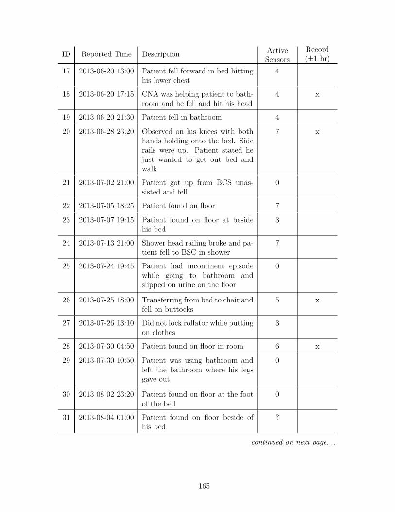
ID Reported Time Description ActiveSensors
Record(±1 hr)
17 2013-06-20 13:00 Patient fell forward in bed hittinghis lower chest
4
18 2013-06-20 17:15 CNA was helping patient to bath-room and he fell and hit his head
4 x
19 2013-06-20 21:30 Patient fell in bathroom 4
20 2013-06-28 23:20 Observed on his knees with bothhands holding onto the bed. Siderails were up. Patient stated hejust wanted to get out bed andwalk
7 x
21 2013-07-02 21:00 Patient got up from BCS unas-sisted and fell
0
22 2013-07-05 18:25 Patient found on floor 7
23 2013-07-07 19:15 Patient found on floor at besidehis bed
3
24 2013-07-13 21:00 Shower head railing broke and pa-tient fell to BSC in shower
7
25 2013-07-24 19:45 Patient had incontinent episodewhile going to bathroom andslipped on urine on the floor
0
26 2013-07-25 18:00 Transferring from bed to chair andfell on buttocks
5 x
27 2013-07-26 13:10 Did not lock rollator while puttingon clothes
3
28 2013-07-30 04:50 Patient found on floor in room 6 x
29 2013-07-30 10:50 Patient was using bathroom andleft the bathroom where his legsgave out
0
30 2013-08-02 23:20 Patient found on floor at the footof the bed
0
31 2013-08-04 01:00 Patient found on floor beside ofhis bed
?
continued on next page. . .
165
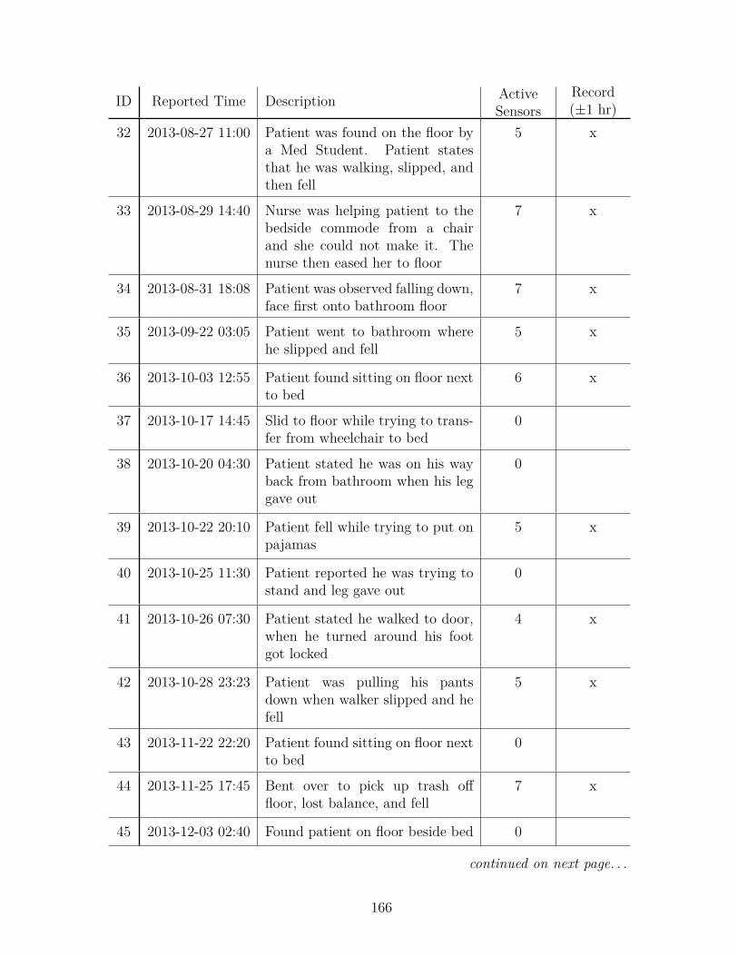
ID Reported Time Description ActiveSensors
Record(±1 hr)
32 2013-08-27 11:00 Patient was found on the floor bya Med Student. Patient statesthat he was walking, slipped, andthen fell
5 x
33 2013-08-29 14:40 Nurse was helping patient to thebedside commode from a chairand she could not make it. Thenurse then eased her to floor
7 x
34 2013-08-31 18:08 Patient was observed falling down,face first onto bathroom floor
7 x
35 2013-09-22 03:05 Patient went to bathroom wherehe slipped and fell
5 x
36 2013-10-03 12:55 Patient found sitting on floor nextto bed
6 x
37 2013-10-17 14:45 Slid to floor while trying to trans-fer from wheelchair to bed
0
38 2013-10-20 04:30 Patient stated he was on his wayback from bathroom when his leggave out
0
39 2013-10-22 20:10 Patient fell while trying to put onpajamas
5 x
40 2013-10-25 11:30 Patient reported he was trying tostand and leg gave out
0
41 2013-10-26 07:30 Patient stated he walked to door,when he turned around his footgot locked
4 x
42 2013-10-28 23:23 Patient was pulling his pantsdown when walker slipped and hefell
5 x
43 2013-11-22 22:20 Patient found sitting on floor nextto bed
0
44 2013-11-25 17:45 Bent over to pick up trash offfloor, lost balance, and fell
7 x
45 2013-12-03 02:40 Found patient on floor beside bed 0
continued on next page. . .
166
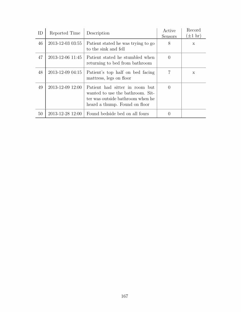
ID Reported Time Description ActiveSensors
Record(±1 hr)
46 2013-12-03 03:55 Patient stated he was trying to goto the sink and fell
8 x
47 2013-12-06 11:45 Patient stated he stumbled whenreturning to bed from bathroom
0
48 2013-12-09 04:15 Patient’s top half on bed facingmattress, legs on floor
7 x
49 2013-12-09 12:00 Patient had sitter in room butwanted to use the bathroom. Sit-ter was outside bathroom when heheard a thump. Found on floor
0
50 2013-12-28 12:00 Found bedside bed on all fours 0
167

Appendix B
Captured Human Fall Acceleration Records
The following are acceleration versus time plots of the signals corresponding to
events highlighted in Table 2.2 that were recorded using sensors in the flooring. Sensor
signals showing little to no data are not displayed. The full list of reported falls and
their descriptions are found in Table A.1.
B.1 Fall Reported on 2013-06-17 22:00 (ID 16)
0 2 4 6 8 10 12Time (s)
−0.03
−0.02
−0.01
0.00
0.01
0.02
0.03
0.04
Acce
lerat
ion
(g)
Figure B.1: Fall Event 2013-06-17 21:57:19 | Sensor D4E1
168

0 2 4 6 8 10 12Time (s)
−0.06
−0.04
−0.02
0.00
0.02
Acce
lerat
ion
(g)
Figure B.2: Fall Event 2013-06-17 21:57:19 | Sensor B3B0
0 2 4 6 8 10 12Time (s)
−0.015
−0.010
−0.005
0.000
0.005
0.010
Acce
lerat
ion
(g)
Figure B.3: Fall Event 2013-06-17 21:58:54 | Sensor BB46
169

0 2 4 6 8 10 12Time (s)
−0.025
−0.020
−0.015
−0.010
−0.005
0.000
0.005
0.010
0.015
Acce
lerat
ion
(g)
Figure B.4: Fall Event 2013-06-17 21:58:54 | Sensor BB87
0 2 4 6 8 10 12Time (s)
−0.5
−0.4
−0.3
−0.2
−0.1
0.0
0.1
0.2
Acce
lerat
ion
(g)
Figure B.5: Fall Event 2013-06-17 22:03:19 | Sensor BB87
170
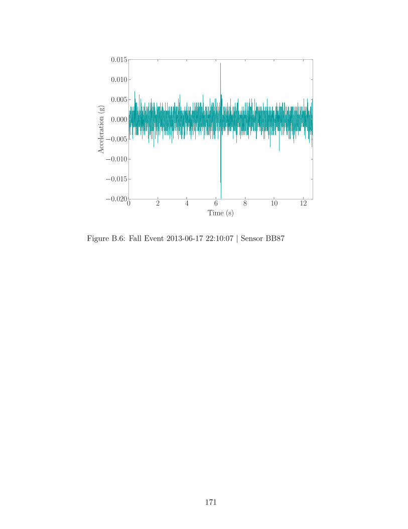
0 2 4 6 8 10 12Time (s)
−0.020
−0.015
−0.010
−0.005
0.000
0.005
0.010
0.015
Acce
lerat
ion
(g)
Figure B.6: Fall Event 2013-06-17 22:10:07 | Sensor BB87
171

B.2 Fall Reported on 2013-06-20 17:15 (ID 18)
0 2 4 6 8 10 12Time (s)
−0.025
−0.020
−0.015
−0.010
−0.005
0.000
0.005
0.010
0.015
Acce
lerat
ion
(g)
Figure B.7: Fall Event 2013-06-20 17:14:23 | Sensor D4E1
0 2 4 6 8 10 12Time (s)
−0.010
−0.005
0.000
0.005
0.010
0.015
Acce
lerat
ion
(g)
Figure B.8: Fall Event 2013-06-20 17:14:23 | Sensor BB46
172

B.3 Fall Reported on 2013-06-28 23:20 (ID 20)
0 2 4 6 8 10 12Time (s)
−0.08
−0.06
−0.04
−0.02
0.00
0.02
0.04
0.06
0.08
0.10
Acce
lerat
ion
(g)
Figure B.9: Fall Event 2013-06-28 23:23:57 | Sensor 8D2C
0 2 4 6 8 10 12Time (s)
−0.10
−0.05
0.00
0.05
0.10
0.15
0.20
0.25
0.30
Acce
lerat
ion
(g)
Figure B.10: Fall Event 2013-06-28 23:24:42 | Sensor 8D2C
173
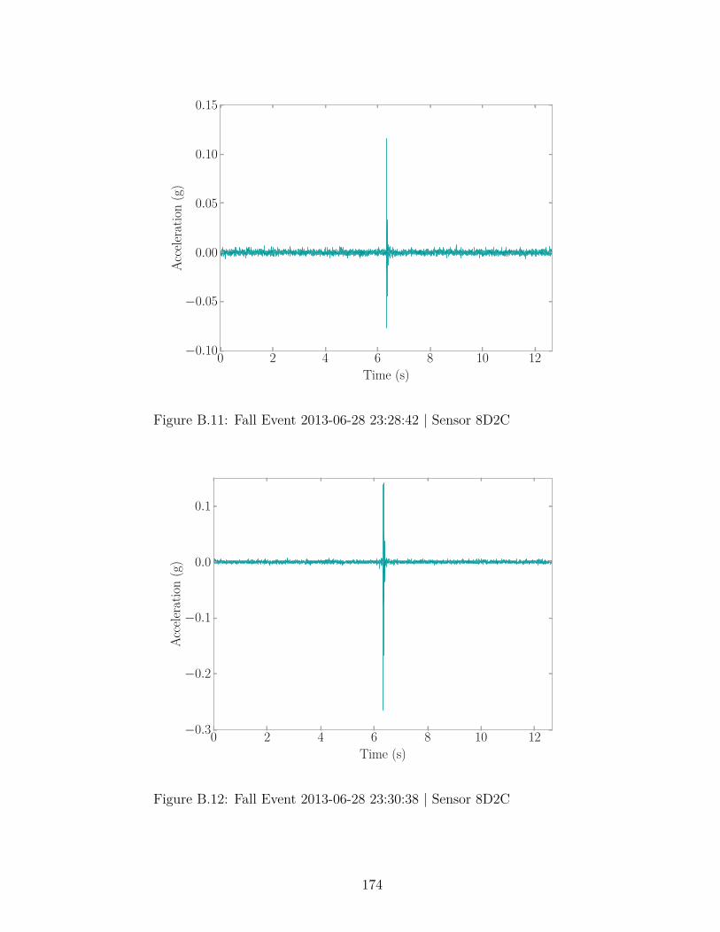
0 2 4 6 8 10 12Time (s)
−0.10
−0.05
0.00
0.05
0.10
0.15
Acce
lerat
ion
(g)
Figure B.11: Fall Event 2013-06-28 23:28:42 | Sensor 8D2C
0 2 4 6 8 10 12Time (s)
−0.3
−0.2
−0.1
0.0
0.1
Acce
lerat
ion
(g)
Figure B.12: Fall Event 2013-06-28 23:30:38 | Sensor 8D2C
174

B.4 Fall Reported on 2013-07-25 18:00 (ID 26)
0 2 4 6 8 10 12Time (s)
−0.03
−0.02
−0.01
0.00
0.01
0.02
0.03
Acce
lerat
ion
(g)
Figure B.13: Fall Event 2013-07-25 17:49:29 | Sensor B3A1
0 2 4 6 8 10 12Time (s)
−0.010
−0.005
0.000
0.005
0.010
0.015
Acce
lerat
ion
(g)
Figure B.14: Fall Event 2013-07-25 17:49:29 | Sensor BB7E
175
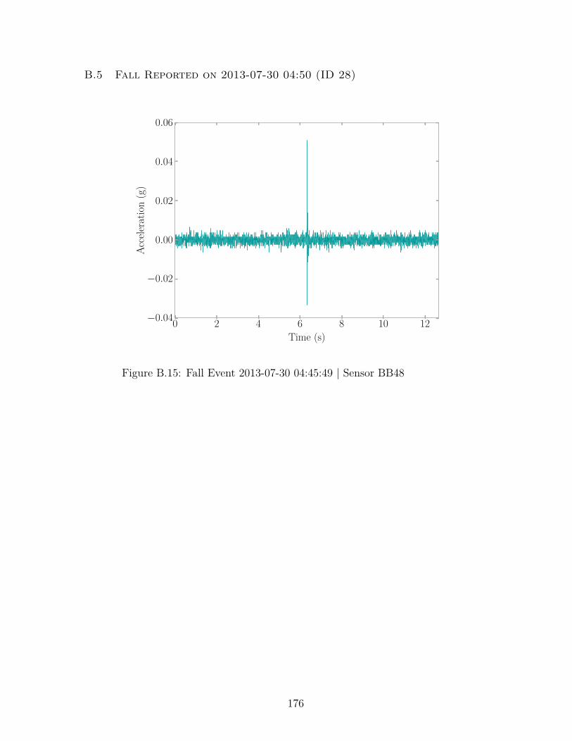
B.5 Fall Reported on 2013-07-30 04:50 (ID 28)
0 2 4 6 8 10 12Time (s)
−0.04
−0.02
0.00
0.02
0.04
0.06Ac
celer
atio
n(g
)
Figure B.15: Fall Event 2013-07-30 04:45:49 | Sensor BB48
176
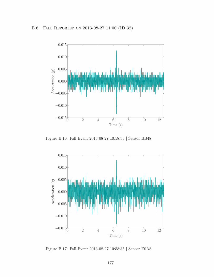
B.6 Fall Reported on 2013-08-27 11:00 (ID 32)
0 2 4 6 8 10 12Time (s)
−0.015
−0.010
−0.005
0.000
0.005
0.010
0.015
Acce
lerat
ion
(g)
Figure B.16: Fall Event 2013-08-27 10:58:35 | Sensor BB48
0 2 4 6 8 10 12Time (s)
−0.015
−0.010
−0.005
0.000
0.005
0.010
0.015
Acce
lerat
ion
(g)
Figure B.17: Fall Event 2013-08-27 10:58:35 | Sensor E0A8
177
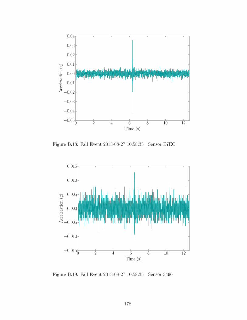
0 2 4 6 8 10 12Time (s)
−0.05
−0.04
−0.03
−0.02
−0.01
0.00
0.01
0.02
0.03
0.04
Acce
lerat
ion
(g)
Figure B.18: Fall Event 2013-08-27 10:58:35 | Sensor E7EC
0 2 4 6 8 10 12Time (s)
−0.015
−0.010
−0.005
0.000
0.005
0.010
0.015
Acce
lerat
ion
(g)
Figure B.19: Fall Event 2013-08-27 10:58:35 | Sensor 3496
178
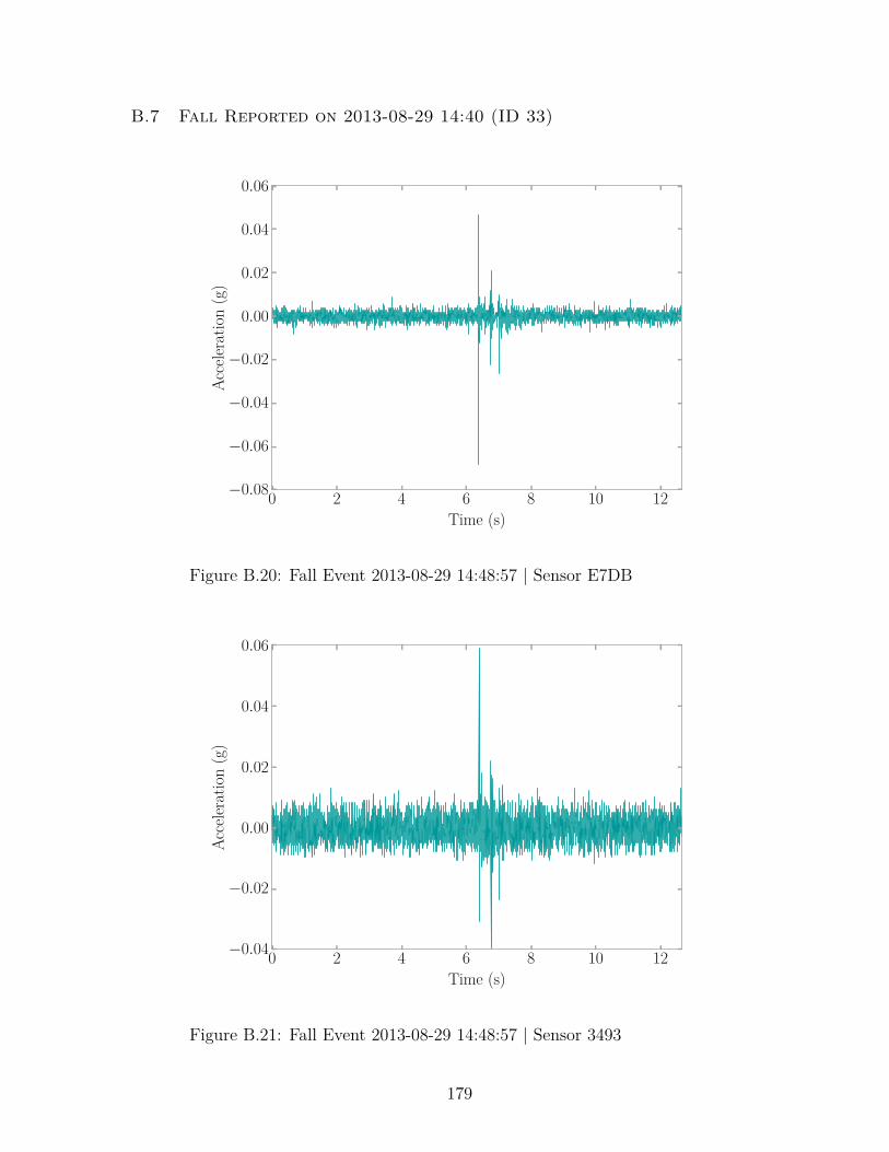
B.7 Fall Reported on 2013-08-29 14:40 (ID 33)
0 2 4 6 8 10 12Time (s)
−0.08
−0.06
−0.04
−0.02
0.00
0.02
0.04
0.06
Acce
lerat
ion
(g)
Figure B.20: Fall Event 2013-08-29 14:48:57 | Sensor E7DB
0 2 4 6 8 10 12Time (s)
−0.04
−0.02
0.00
0.02
0.04
0.06
Acce
lerat
ion
(g)
Figure B.21: Fall Event 2013-08-29 14:48:57 | Sensor 3493
179
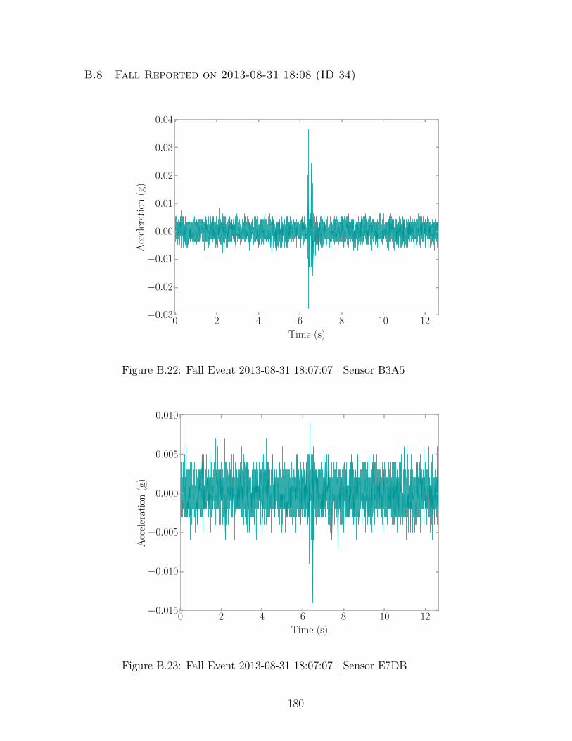
B.8 Fall Reported on 2013-08-31 18:08 (ID 34)
0 2 4 6 8 10 12Time (s)
−0.03
−0.02
−0.01
0.00
0.01
0.02
0.03
0.04
Acce
lerat
ion
(g)
Figure B.22: Fall Event 2013-08-31 18:07:07 | Sensor B3A5
0 2 4 6 8 10 12Time (s)
−0.015
−0.010
−0.005
0.000
0.005
0.010
Acce
lerat
ion
(g)
Figure B.23: Fall Event 2013-08-31 18:07:07 | Sensor E7DB
180

0 2 4 6 8 10 12Time (s)
−0.03
−0.02
−0.01
0.00
0.01
0.02
0.03
0.04
0.05
0.06
Acce
lerat
ion
(g)
Figure B.24: Fall Event 2013-08-31 18:07:07 | Sensor 8D2C
181

B.9 Fall Reported on 2013-09-22 03:05 (ID 35)
0 2 4 6 8 10 12Time (s)
−0.02
−0.01
0.00
0.01
0.02
0.03
0.04
0.05
Acce
lerat
ion
(g)
Figure B.25: Fall Event 2013-09-22 02:45:21 | Sensor C7AE
0 2 4 6 8 10 12Time (s)
−0.04
−0.02
0.00
0.02
0.04
Acce
lerat
ion
(g)
Figure B.26: Fall Event 2013-09-22 02:45:21 | Sensor DC67
182

0 2 4 6 8 10 12Time (s)
−0.03
−0.02
−0.01
0.00
0.01
0.02
0.03
0.04
0.05
Acce
lerat
ion
(g)
Figure B.27: Fall Event 2013-09-22 02:45:21 | Sensor 2E73
183

B.10 Fall Reported on 2013-10-03 12:55 (ID 36)
0 2 4 6 8 10 12Time (s)
−0.020
−0.015
−0.010
−0.005
0.000
0.005
0.010
0.015
0.020
0.025
Acce
lerat
ion
(g)
Figure B.28: Fall Event 2013-10-03 12:34:31 | Sensor B3A5
184

B.11 Fall Reported on 2013-10-22 20:10 (ID 39)
0 2 4 6 8 10 12Time (s)
−0.03
−0.02
−0.01
0.00
0.01
0.02
0.03Ac
celer
atio
n(g
)
Figure B.29: Fall Event 2013-10-22 20:02:20 | Sensor E7EC
185
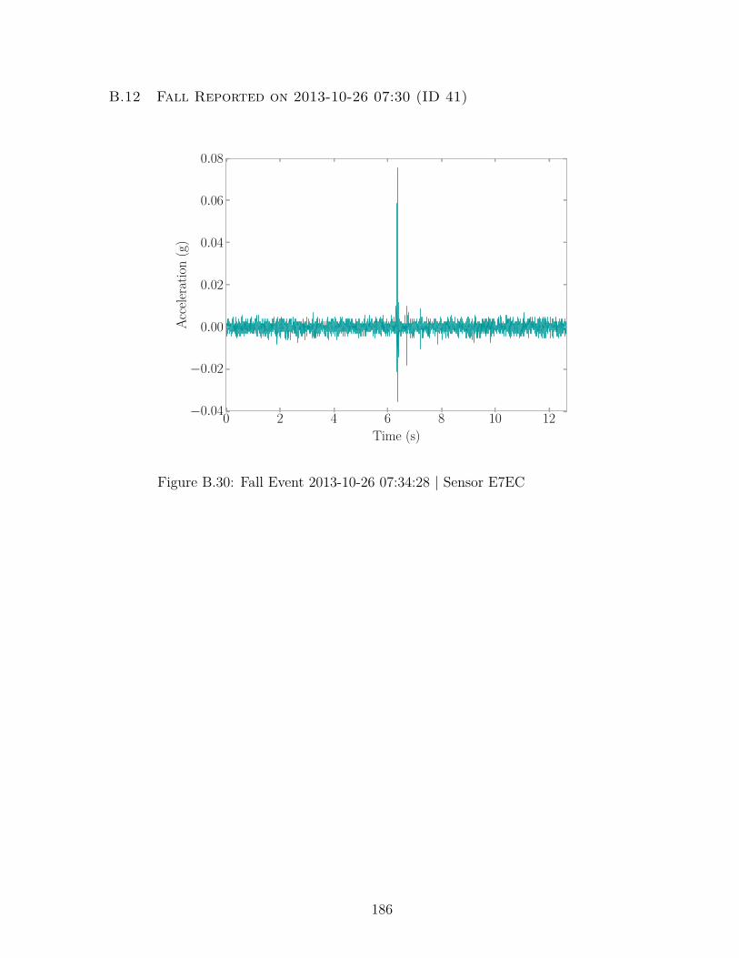
B.12 Fall Reported on 2013-10-26 07:30 (ID 41)
0 2 4 6 8 10 12Time (s)
−0.04
−0.02
0.00
0.02
0.04
0.06
0.08Ac
celer
atio
n(g
)
Figure B.30: Fall Event 2013-10-26 07:34:28 | Sensor E7EC
186

B.13 Fall Reported on 2013-10-28 23:23 (ID 42)
0 2 4 6 8 10 12Time (s)
−0.020
−0.015
−0.010
−0.005
0.000
0.005
0.010
0.015
0.020
0.025
Acce
lerat
ion
(g)
Figure B.31: Fall Event 2013-10-28 23:25:33 | Sensor E0A8
187
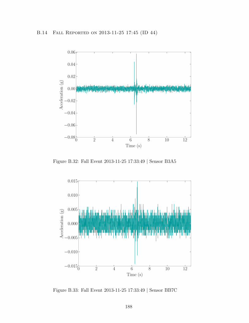
B.14 Fall Reported on 2013-11-25 17:45 (ID 44)
0 2 4 6 8 10 12Time (s)
−0.08
−0.06
−0.04
−0.02
0.00
0.02
0.04
0.06
Acce
lerat
ion
(g)
Figure B.32: Fall Event 2013-11-25 17:33:49 | Sensor B3A5
0 2 4 6 8 10 12Time (s)
−0.015
−0.010
−0.005
0.000
0.005
0.010
0.015
Acce
lerat
ion
(g)
Figure B.33: Fall Event 2013-11-25 17:33:49 | Sensor BB7C
188

0 2 4 6 8 10 12Time (s)
−0.10
−0.08
−0.06
−0.04
−0.02
0.00
0.02
0.04
0.06
0.08
Acce
lerat
ion
(g)
Figure B.34: Fall Event 2013-11-25 17:33:49 | Sensor 3087
0 2 4 6 8 10 12Time (s)
−0.04
−0.03
−0.02
−0.01
0.00
0.01
0.02
0.03
0.04
0.05
Acce
lerat
ion
(g)
Figure B.35: Fall Event 2013-11-25 17:33:49 | Sensor 3493
189
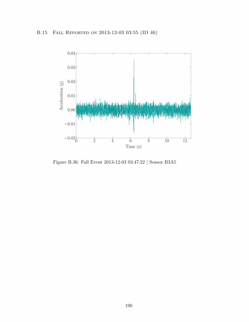
B.15 Fall Reported on 2013-12-03 03:55 (ID 46)
0 2 4 6 8 10 12Time (s)
−0.02
−0.01
0.00
0.01
0.02
0.03
0.04Ac
celer
atio
n(g
)
Figure B.36: Fall Event 2013-12-03 03:47:22 | Sensor B3A5
190

B.16 Fall Reported on 2013-12-09 04:15 (ID 48)
0 2 4 6 8 10 12Time (s)
−0.025
−0.020
−0.015
−0.010
−0.005
0.000
0.005
0.010
0.015
Acce
lerat
ion
(g)
Figure B.37: Fall Event 2013-12-09 04:59:04 | Sensor B3A5
0 2 4 6 8 10 12Time (s)
−0.10
−0.08
−0.06
−0.04
−0.02
0.00
0.02
0.04
Acce
lerat
ion
(g)
Figure B.38: Fall Event 2013-12-09 04:59:04 | Sensor BB45
191
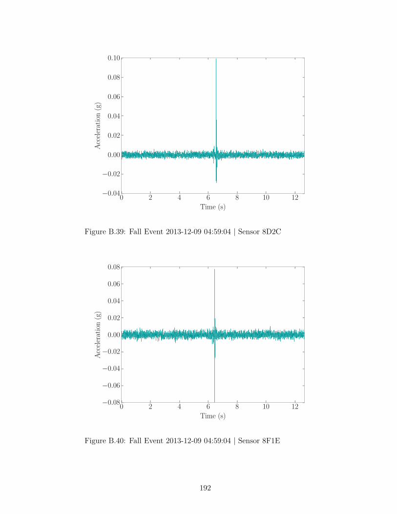
0 2 4 6 8 10 12Time (s)
−0.04
−0.02
0.00
0.02
0.04
0.06
0.08
0.10
Acce
lerat
ion
(g)
Figure B.39: Fall Event 2013-12-09 04:59:04 | Sensor 8D2C
0 2 4 6 8 10 12Time (s)
−0.08
−0.06
−0.04
−0.02
0.00
0.02
0.04
0.06
0.08
Acce
lerat
ion
(g)
Figure B.40: Fall Event 2013-12-09 04:59:04 | Sensor 8F1E
192

Appendix C
Sample Human Activity Database Queries
The following presents example Human Activity Database queries grouped by
informational type. This is part of the data management plan discussed in Chapter 3.
C.1 Database Table Information
Getting a list of column names in a database table. If another table is desired, simply
replace accel_events with your desired table.
Code Snippet C.1: List Columns of a Table
SELECT COLUMN_NAMEFROM INFORMATION_SCHEMA.COLUMNSWHERE TABLE_SCHEMA = "main_ssh"
AND TABLE_NAME = "accel_events";
C.2 Sensor Related Queries
Find calibration records for a particular sensor. Replace the sensor_mac value with
the Media Access Control Address (MAC Address) of the sensor desired.
Code Snippet C.2: Find The Calibration Record of a Sensor
SELECT *FROM calibrationWHERE sensor_mac = "0006661495C0";
193
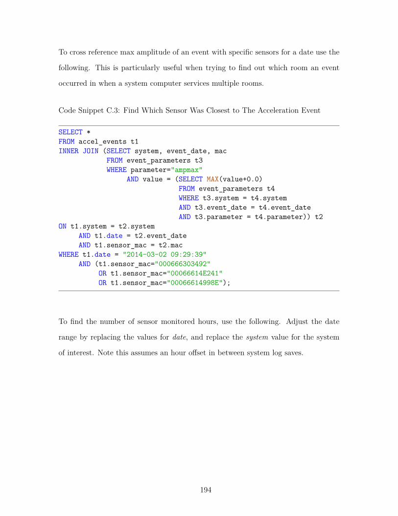
To cross reference max amplitude of an event with specific sensors for a date use the
following. This is particularly useful when trying to find out which room an event
occurred in when a system computer services multiple rooms.
Code Snippet C.3: Find Which Sensor Was Closest to The Acceleration Event
SELECT *FROM accel_events t1INNER JOIN (SELECT system, event_date, mac
FROM event_parameters t3WHERE parameter="ampmax"
AND value = (SELECT MAX(value+0.0)FROM event_parameters t4WHERE t3.system = t4.systemAND t3.event_date = t4.event_dateAND t3.parameter = t4.parameter)) t2
ON t1.system = t2.systemAND t1.date = t2.event_dateAND t1.sensor_mac = t2.mac
WHERE t1.date = "2014-03-02 09:29:39"AND (t1.sensor_mac="000666303492"
OR t1.sensor_mac="00066614E241"OR t1.sensor_mac="00066614998E");
To find the number of sensor monitored hours, use the following. Adjust the date
range by replacing the values for date, and replace the system value for the system
of interest. Note this assumes an hour offset in between system log saves.
194
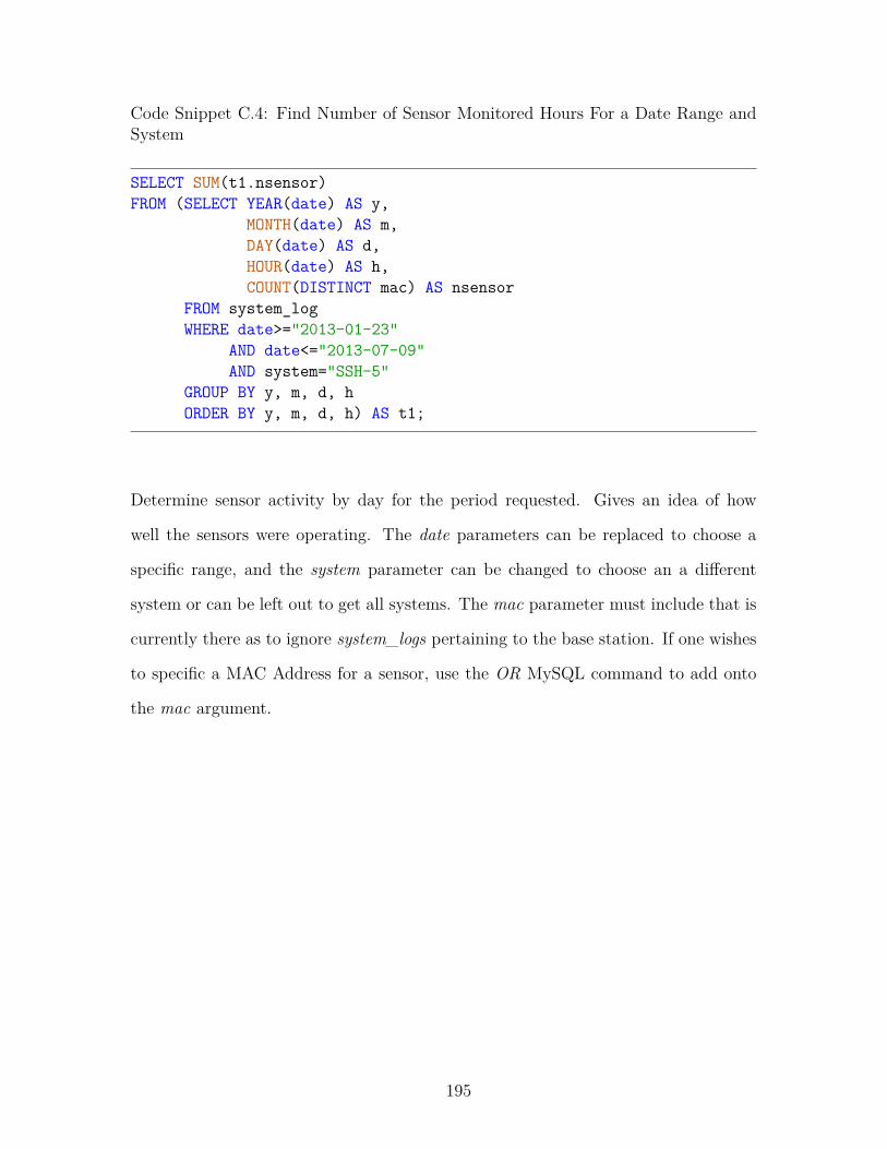
Code Snippet C.4: Find Number of Sensor Monitored Hours For a Date Range andSystem
SELECT SUM(t1.nsensor)FROM (SELECT YEAR(date) AS y,
MONTH(date) AS m,DAY(date) AS d,HOUR(date) AS h,COUNT(DISTINCT mac) AS nsensor
FROM system_logWHERE date>="2013-01-23"
AND date<="2013-07-09"AND system="SSH-5"
GROUP BY y, m, d, hORDER BY y, m, d, h) AS t1;
Determine sensor activity by day for the period requested. Gives an idea of how
well the sensors were operating. The date parameters can be replaced to choose a
specific range, and the system parameter can be changed to choose an a different
system or can be left out to get all systems. The mac parameter must include that is
currently there as to ignore system_logs pertaining to the base station. If one wishes
to specific a MAC Address for a sensor, use the OR MySQL command to add onto
the mac argument.
195
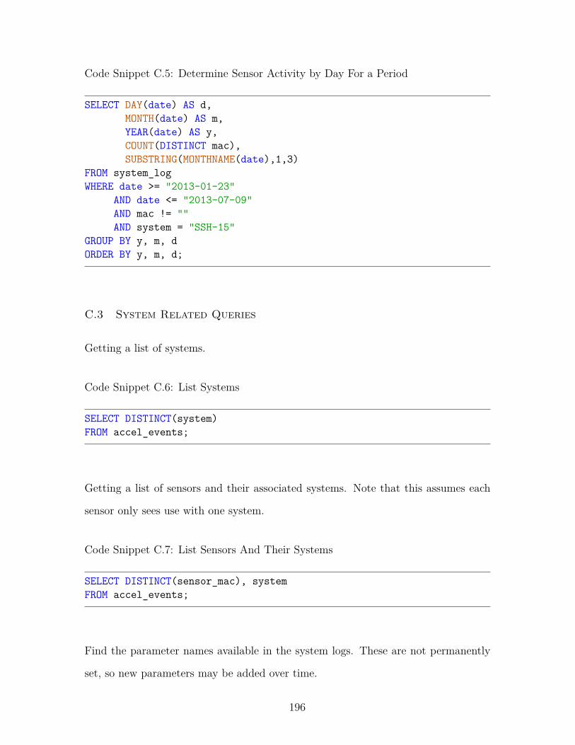
Code Snippet C.5: Determine Sensor Activity by Day For a Period
SELECT DAY(date) AS d,MONTH(date) AS m,YEAR(date) AS y,COUNT(DISTINCT mac),SUBSTRING(MONTHNAME(date),1,3)
FROM system_logWHERE date >= "2013-01-23"
AND date <= "2013-07-09"AND mac != ""AND system = "SSH-15"
GROUP BY y, m, dORDER BY y, m, d;
C.3 System Related Queries
Getting a list of systems.
Code Snippet C.6: List Systems
SELECT DISTINCT(system)FROM accel_events;
Getting a list of sensors and their associated systems. Note that this assumes each
sensor only sees use with one system.
Code Snippet C.7: List Sensors And Their Systems
SELECT DISTINCT(sensor_mac), systemFROM accel_events;
Find the parameter names available in the system logs. These are not permanently
set, so new parameters may be added over time.
196

Code Snippet C.8: Available System Log Parameters
SELECT DISTINCT(parameter)FROM system_log;
Access system logs for a particular sensor.
Code Snippet C.9: Access System Logs For a Sensor
SELECT *FROM system_logWHERE mac = "00066614B3A1";
Access system logs for the system base station.
Code Snippet C.10: Access System Logs For a Sensor
SELECT *FROM system_logWHERE system = "SSH-36"AND mac = "";
Access download information for a particular system. Gives insight into how the data
was sent to the database.
Code Snippet C.11: Access Download Information For a System
SELECT *FROM downloadsWHERE system = "SSH-5";
197
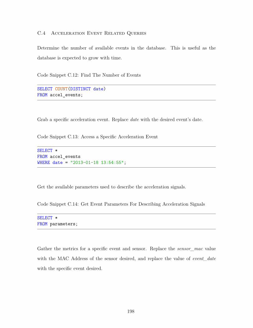
C.4 Acceleration Event Related Queries
Determine the number of available events in the database. This is useful as the
database is expected to grow with time.
Code Snippet C.12: Find The Number of Events
SELECT COUNT(DISTINCT date)FROM accel_events;
Grab a specific acceleration event. Replace date with the desired event’s date.
Code Snippet C.13: Access a Specific Acceleration Event
SELECT *FROM accel_eventsWHERE date = "2013-01-18 13:54:55";
Get the available parameters used to describe the acceleration signals.
Code Snippet C.14: Get Event Parameters For Describing Acceleration Signals
SELECT *FROM parameters;
Gather the metrics for a specific event and sensor. Replace the sensor_mac value
with the MAC Address of the sensor desired, and replace the value of event_date
with the specific event desired.
198

Code Snippet C.15: Find the Signal Metrics For an Event and Sensor
SELECT *FROM event_parametersWHERE mac = "00066614B3AA"
AND event_date = "2013-07-20 02:44:25";
To find a flat signal (i.e. one with little to no excitation), set the amplitude value low
for ampmax like in the following.
Code Snippet C.16: Find a Flat Acceleration Signal
SELECT t1.*, t2.value AS ampmaxFROM accel_events t1INNER JOIN event_parameters t2 ON m1.date = t2.event_date
AND t1.sensor_mac = t2.macWHERE t2.parameter = "ampmax"
AND t2.value < 0.0125;
Find a spike signal (i.e. a sensor error that reads only one high value). See Sec-
tion 2.4.2 for more details.
Code Snippet C.17: Find a Spike Acceleration Signal
SELECT t1.*FROM event_parameters t1INNER JOIN event_parameters t2 ON t1.event_date = t2.event_date
AND t1.mac = t2.macINNER JOIN accel_events ON accel_events.date = t1.event_date
AND accel_events.sensor_mac = t1.macWHERE t1.parameter = "metric1"
AND t2.parameter = "ampmax"AND t2.value > 0.5AND t1.value/t2.value > 0.95;
199

Find the maximum parameter value for a period, simply replace ampmax with the
desired parameter, replace the event_date ranges, and replace the system.
Code Snippet C.18: Find Maximum Parameter Value For a System and Date Range
SELECT tt.*FROM event_parameters ttINNER JOIN (SELECT system,
event_date,mac,parameter,MAX(value+0.0) AS MaxVal
FROM event_parametersWHERE parameter= "ampmax"
AND event_date >= "2013-01-18"AND event_date <= "2014-06-14"AND system = "SSH-36"
GROUP BY event_date) groupedttON tt.event_date = groupedtt.event_date
AND tt.value = groupedtt.MaxValORDER BY event_date;
Getting the number of events by day can give a sense of how activity is distributed
across a period of time. The date parameters can be replaced to choose a specific
range, and the system parameter can be changed to choose an a different system or
can be left out to get all systems. The mac parameter must include that is currently
there as to ignore system_logs pertaining to the base station. If one wishes to specific
a MAC Address for a sensor, use the OR MySQL command to add onto the mac
argument.
200
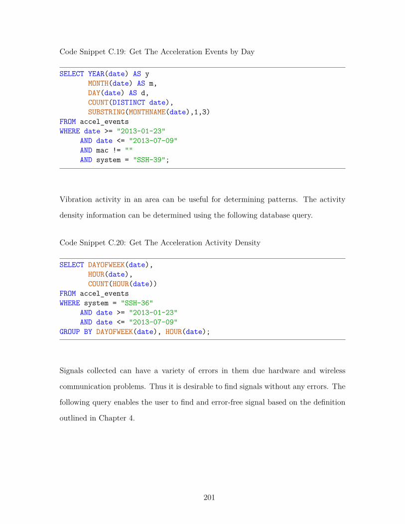
Code Snippet C.19: Get The Acceleration Events by Day
SELECT YEAR(date) AS yMONTH(date) AS m,DAY(date) AS d,COUNT(DISTINCT date),SUBSTRING(MONTHNAME(date),1,3)
FROM accel_eventsWHERE date >= "2013-01-23"
AND date <= "2013-07-09"AND mac != ""AND system = "SSH-39";
Vibration activity in an area can be useful for determining patterns. The activity
density information can be determined using the following database query.
Code Snippet C.20: Get The Acceleration Activity Density
SELECT DAYOFWEEK(date),HOUR(date),COUNT(HOUR(date))
FROM accel_eventsWHERE system = "SSH-36"
AND date >= "2013-01-23"AND date <= "2013-07-09"
GROUP BY DAYOFWEEK(date), HOUR(date);
Signals collected can have a variety of errors in them due hardware and wireless
communication problems. Thus it is desirable to find signals without any errors. The
following query enables the user to find and error-free signal based on the definition
outlined in Chapter 4.
201

Code Snippet C.21: Find Error-Free Signals
SELECT ae.sensor_mac, ae.date, ae.dataFROM accel_events aeWHERE NOT EXISTS (
SELECT NULLFROM event_parameters ep1INNER JOIN event_parameters ep2
ON ep1.mac = ep2.macAND ep1.event_date = ep2.event_date
INNER JOIN event_parameters ep3ON ep1.mac = ep3.macAND ep1.event_date = ep3.event_date
WHERE ae.date = ep1.event_dateAND ae.sensor_mac = ep1.macAND ep1.parameter = "nandensity"AND ep2.parameter = "ampmax"AND ep3.parameter = "mad"AND (ep1.value+0.0 > 0.0
OR (ep3.value+0.0)/(ep2.value+0.0) > 0.95OR LOWER(ep2.value) = "nan"OR LOWER(ep3.value) = "nan")
)AND ae.data <> ’No Data’
202
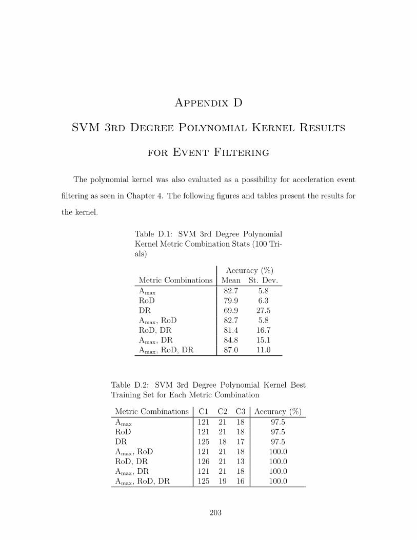
Appendix D
SVM 3rd Degree Polynomial Kernel Results
for Event Filtering
The polynomial kernel was also evaluated as a possibility for acceleration event
filtering as seen in Chapter 4. The following figures and tables present the results for
the kernel.
Table D.1: SVM 3rd Degree PolynomialKernel Metric Combination Stats (100 Tri-als)
Accuracy (%)Metric Combinations Mean St. Dev.Amax 82.7 5.8RoD 79.9 6.3DR 69.9 27.5Amax, RoD 82.7 5.8RoD, DR 81.4 16.7Amax, DR 84.8 15.1Amax, RoD, DR 87.0 11.0
Table D.2: SVM 3rd Degree Polynomial Kernel BestTraining Set for Each Metric Combination
Metric Combinations C1 C2 C3 Accuracy (%)Amax 121 21 18 97.5RoD 121 21 18 97.5DR 125 18 17 97.5Amax, RoD 121 21 18 100.0RoD, DR 126 21 13 100.0Amax, DR 121 21 18 100.0Amax, RoD, DR 125 19 16 100.0
203

Table D.3: SVM 3rd Degree Polynomial Kernel WorstTraining Set for Each Metric Combination
Metric Combinations C1 C2 C3 Accuracy (%)Amax 134 11 15 67.5RoD 134 15 11 65.0DR 121 21 18 0.0Amax, RoD 134 11 15 67.5RoD, DR 130 17 13 15.0Amax, DR 127 17 16 17.5Amax, RoD, DR 126 21 13 10.0
−9 −7 −5 −3 −1log(RoD)
−6−5−4−3−2−1
01
log(
Am
ax)
0 1 2 3 4 5log(DR)
−9
−7
−5
−3
−1
log(
RoD
)
Category 1Category 2Category 3
Figure D.1: SVM 3rd Degree Polynomial Kernel Metric CombinationHyperplanes
204
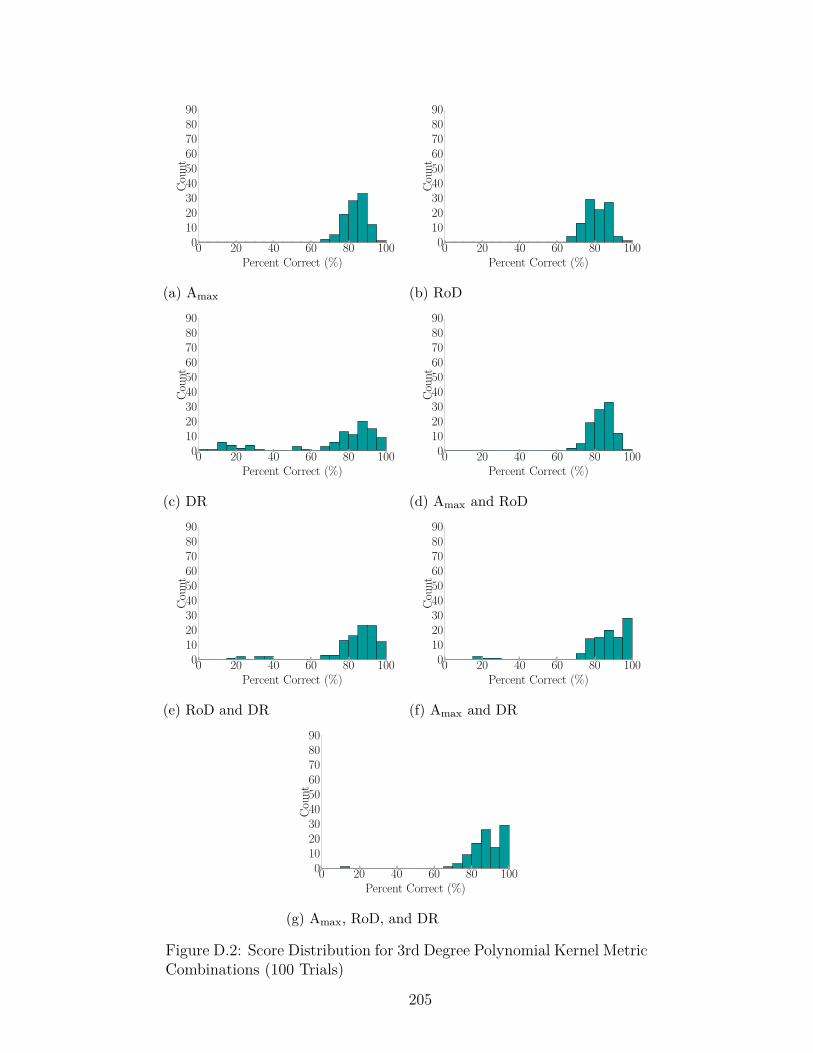
0 20 40 60 80 100Percent Correct (%)
0102030405060708090
Coun
t
(a) Amax
0 20 40 60 80 100Percent Correct (%)
0102030405060708090
Coun
t
(b) RoD
0 20 40 60 80 100Percent Correct (%)
0102030405060708090
Coun
t
(c) DR
0 20 40 60 80 100Percent Correct (%)
0102030405060708090
Coun
t
(d) Amax and RoD
0 20 40 60 80 100Percent Correct (%)
0102030405060708090
Coun
t
(e) RoD and DR
0 20 40 60 80 100Percent Correct (%)
0102030405060708090
Coun
t
(f) Amax and DR
0 20 40 60 80 100Percent Correct (%)
0102030405060708090
Coun
t
(g) Amax, RoD, and DR
Figure D.2: Score Distribution for 3rd Degree Polynomial Kernel MetricCombinations (100 Trials)
205

Appendix E
SVM Sigmoid Kernel Results for Event
Filtering
The sigmoid kernel was also evaluated as a possibility for acceleration event fil-
tering as seen in Chapter 4. The following figures and tables present the results for
the kernel.
Table E.1: SVM Sigmoid Kernel MetricCombination Stats (100 Trials)
Accuracy (%)Metric Combinations Mean St. Dev.Amax 93.6 3.7RoD 81.3 6.1DR 79.9 6.3Amax, RoD 93.4 3.7RoD, DR 79.9 6.3Amax, DR 79.9 6.3Amax, RoD, DR 79.9 6.3
Table E.2: SVM Sigmoid Kernel Best Training Set forEach Metric Combination
Metric Combinations C1 C2 C3 Accuracy (%)Amax 121 21 18 100.0RoD 121 21 18 97.5DR 121 21 18 97.5Amax, RoD 121 21 18 100.0RoD, DR 121 21 18 97.5Amax, DR 121 21 18 97.5Amax, RoD, DR 121 21 18 97.5
206

Table E.3: SVM Sigmoid Kernel Worst Training Set forEach Metric Combination
Metric Combinations C1 C2 C3 Accuracy (%)Amax 132 16 12 82.5RoD 134 11 15 67.5DR 134 15 11 65.0Amax, RoD 132 16 12 82.5RoD, DR 134 15 11 65.0Amax, DR 134 15 11 65.0Amax, RoD, DR 134 15 11 65.0
207

0 20 40 60 80 100Percent Correct (%)
0102030405060708090
Coun
t
(a) Amax
0 20 40 60 80 100Percent Correct (%)
0102030405060708090
Coun
t
(b) RoD
0 20 40 60 80 100Percent Correct (%)
0102030405060708090
Coun
t
(c) DR
0 20 40 60 80 100Percent Correct (%)
0102030405060708090
Coun
t
(d) Amax and RoD
0 20 40 60 80 100Percent Correct (%)
0102030405060708090
Coun
t
(e) RoD and DR
0 20 40 60 80 100Percent Correct (%)
0102030405060708090
Coun
t
(f) Amax and DR
0 20 40 60 80 100Percent Correct (%)
0102030405060708090
Coun
t
(g) Amax, RoD, and DR
Figure E.1: Score Distribution for Sigmoid Kernel Metric Combinations(100 Trials)
208
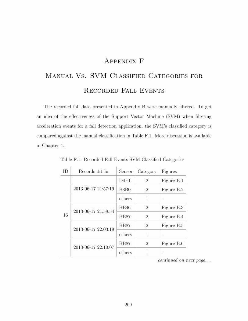
Appendix F
Manual Vs. SVM Classified Categories for
Recorded Fall Events
The recorded fall data presented in Appendix B were manually filtered. To get
an idea of the effectiveness of the Support Vector Machine (SVM) when filtering
acceleration events for a fall detection application, the SVM’s classified category is
compared against the manual classification in Table F.1. More discussion is available
in Chapter 4.
Table F.1: Recorded Fall Events SVM Classified Categories
ID Records ±1 hr Sensor Category Figures
16
2013-06-17 21:57:19D4E1 2 Figure B.1
B3B0 2 Figure B.2
others 1 -
2013-06-17 21:58:54BB46 2 Figure B.3
BB87 2 Figure B.4
2013-06-17 22:03:19BB87 2 Figure B.5
others 1 -
2013-06-17 22:10:07BB87 2 Figure B.6
others 1 -continued on next page. . .
209

ID Records ±1 hr Sensor Category Figures
18 2013-06-20 17:14:23D4E1 2 Figure B.7
BB46 2 Figure B.8
others 1 -
20
2013-06-28 23:23:578D2C 3 Figure B.9
others 1 -
2013-06-28 23:24:428D2C - Figure B.10
others 1 -
2013-06-28 23:28:428D2C - Figure B.11
others 1 -
2013-06-28 23:30:388D2C 3 Figure B.12
others 1 -
26 2013-07-25 17:49:29B3A1 2 Figure B.13
BB7E - Figure B.14
others 1 -
28 2013-07-30 04:45:49BB48 3 Figure B.15
others 1 -
32 2013-08-27 10:58:35
BB48 2 Figure B.16
E0A8 2 Figure B.17
E7EC 3 Figure B.18
3496 1 Figure B.19
others 1 -
33 2013-08-29 14:48:57E7DB 3 Figure B.20
3493 2 Figure B.21
others 1 or 2 -
34 2013-08-31 18:07:07
B3A5 2 Figure B.22
E7DB - Figure B.23
8D2C - Figure B.24
others 1 -continued on next page. . .
210

ID Records ±1 hr Sensor Category Figures
35 2013-09-22 02:45:21
C7AE 3 Figure B.25
DC67 3 Figure B.26
2E73 3 Figure B.27
others - -
36 2013-10-03 12:34:31B3A5 2 Figure B.28
others 1 -
39 2013-10-22 20:02:20E7EC - Figure B.29
others 1 -
41 2013-10-26 07:34:28E7EC - Figure B.30
others 2 -
42 2013-10-28 23:25:33E0A8 2 Figure B.31
others - -
44 2013-11-25 17:33:49
B3A5 3 Figure B.32
BB7C 2 Figure B.33
3087 3 Figure B.34
3493 2 Figure B.35
others 2 -
46 2013-12-03 03:47:22B3A5 2 Figure B.36
others 1,2 -
48 2013-12-09 04:59:04
B3A5 2 Figure B.37
BB45 3 Figure B.38
8D2C 3 Figure B.39
8F1E - Figure B.40
others 1 -
211
Appendix G
Event Localization Method Attempts
This section describes the attempted methods towards determine the location
of an impact from a force estimate generated by Equation 5.5 whilst developing
the FEEL Algorithm. All methods have the flexibility of window choice like in the
Correlated Force Estimates Method of Section 5.2.3.
G.1 Deviation Method
Following the selection of a window, the standard deviation is taken between the
resulting real portions of the force estimations from each sensor to each location,
point by point within the window. Equation G.1 demonstrates this step with {Li}
being a vector of maximum standard deviations σ for each location, F̂i,j(k) being
the force estimate for the i-th location and j-th sensor, k being the point within the
force estimate vector being compared, and n being the number of points in the force
estimate window.
{Li} = max
σ( F̂i,1(k) F̂i,2(k) · · · F̂i,j(k) )
σ( F̂i,1(k + 1) F̂i,2(k + 1) · · · F̂i,j(k + 1) )... ... ... . . . ...
σ( F̂i,1(k + n) F̂i,2(k + n) · · · F̂i,j(k + n) )
(G.1)
The maximum standard deviation of the force at each location is then compared
in Equation G.2 where L̂ is the lowest standard deviation, which indicates the impact
212

location estimation, and min() is the minimum value function.
L̂ = min({Li}) (G.2)
The reasoning is that the location’s force estimates that more closely match in
magnitude for the specified window, indicates the location of impact. This works
very well for impulse forces, but begins to have challenges when applied to other
force impacts such as a person jumping as seen in the following tables.
Table G.1: Confusion Matrix for Locating Ball-Low Impacts Using The DeviationMethod
IdentifiedLocation 1 Location 2 Location 3 Location 4 Location 5
Act
ual
Location 1 100 0 0 0 0Location 2 0 100 0 0 0Location 3 0 0 100 0 0Location 4 0 0 0 100 0Location 5 0 1 0 0 99
Table G.2: Confusion Matrix for Locating Ball-High Impacts Using The DeviationMethod
IdentifiedLocation 1 Location 2 Location 3 Location 4 Location 5
Act
ual
Location 1 100 0 0 0 0Location 2 0 100 0 0 0Location 3 0 1 99 0 0Location 4 0 0 0 100 0Location 5 0 0 0 0 100
213

Table G.3: Confusion Matrix for Locating Bag-Low Impacts Using The DeviationMethod
IdentifiedLocation 1 Location 2 Location 3 Location 4 Location 5
Act
ual
Location 1 91 0 0 9 0Location 2 2 98 0 0 0Location 3 60 0 4 36 0Location 4 1 1 0 98 0Location 5 20 65 0 0 15
Table G.4: Confusion Matrix for Locating Bag-High Impacts Using The DeviationMethod
IdentifiedLocation 1 Location 2 Location 3 Location 4 Location 5
Act
ual
Location 1 84 1 0 15 0Location 2 0 100 0 0 0Location 3 51 0 6 43 0Location 4 2 8 0 90 0Location 5 24 70 0 0 6
Table G.5: Confusion Matrix for Locating D-Jump Impacts Using The DeviationMethod
IdentifiedLocation 1 Location 2 Location 3 Location 4 Location 5
Act
ual
Location 1 89 0 0 9 2Location 2 1 99 0 0 0Location 3 0 0 97 3 0Location 4 0 0 0 100 0Location 5 0 0 0 4 96
214

Table G.6: Confusion Matrix for Locating J-Jump Impacts Using The DeviationMethod
IdentifiedLocation 1 Location 2 Location 3 Location 4 Location 5
Act
ual
Location 1 95 0 1 4 0Location 2 17 79 1 3 0Location 3 1 0 95 4 0Location 4 2 0 0 98 0Location 5 29 10 0 24 37
Table G.7: Confusion Matrix for Locating W-Jump Impacts Using The DeviationMethod
IdentifiedLocation 1 Location 2 Location 3 Location 4 Location 5
Act
ual
Location 1 54 0 0 46 0Location 2 86 11 0 3 0Location 3 30 0 56 14 0Location 4 0 0 0 100 0Location 5 34 0 0 53 13
G.2 Deviation of Normalized Force Estimates
This method is similar to the Deviation Method discussed in Section G.1, but
normalizes the force before making the standard deviation calculations. Equation G.3
normalizes each force estimate where F̂i,j is the force estimate for the i-th location
and j-th sensor, and max() is the maximum value function.
||F̂i,j|| = F̂i,j
max(∣∣∣F̂i,j
∣∣∣) (G.3)
The standard deviation is then taken point by point for a chosen window in
Equation G.4 where {Li} is a vector of maximum standard deviations σ for each
location, ||F̂i,j|| being the normalized force estimate for the i-th location and j-th
215

sensor, k being the point within the force estimate vector being compared, and n
being the number of points in the normalized force estimate window.
{Li} = max
σ( ||F̂i,1(k)|| ||F̂i,2(k)|| · · · ||F̂i,j(k)|| )
σ( ||F̂i,1(k + 1)|| ||F̂i,2(k + 1)|| · · · ||F̂i,j(k + 1)|| )... ... ... . . . ...
σ( ||F̂i,1(k + n)|| ||F̂i,2(k + n)|| · · · ||F̂i,j(k + n)|| )
(G.4)
Finally, the location is identified as being the location with lowest standard devi-
ation value as seen in Equation G.5.
L̂ = min({Li}) (G.5)
Since the peak magnitudes varied a lot between the sensors, the thought became
to normalized each signal so that the maximum value was one. In theory, this would
move the shapes of the force closer together for the actual location. See the confusion
matrices below for results.
Table G.8: Confusion Matrix for Locating Ball-Low Impacts Using The Deviationof Normalized Force Estimates Method
IdentifiedLocation 1 Location 2 Location 3 Location 4 Location 5
Act
ual
Location 1 100 0 0 0 0Location 2 0 100 0 0 0Location 3 0 0 100 0 0Location 4 0 0 0 100 0Location 5 0 0 0 0 100
216

Table G.9: Confusion Matrix for Locating Ball-High Impacts Using The Deviationof Normalized Force Estimates Method
IdentifiedLocation 1 Location 2 Location 3 Location 4 Location 5
Act
ual
Location 1 100 0 0 0 0Location 2 0 100 0 0 0Location 3 0 1 99 0 0Location 4 0 0 0 100 0Location 5 0 0 0 0 100
Table G.10: Confusion Matrix for Locating Bag-Low Impacts Using The Deviationof Normalized Force Estimates Method
IdentifiedLocation 1 Location 2 Location 3 Location 4 Location 5
Act
ual
Location 1 100 0 0 0 0Location 2 0 96 0 4 0Location 3 0 25 11 55 0Location 4 0 1 0 99 0Location 5 0 3 0 2 95
Table G.11: Confusion Matrix for Locating Bag-High Impacts Using The Deviationof Normalized Force Estimates Method
IdentifiedLocation 1 Location 2 Location 3 Location 4 Location 5
Act
ual
Location 1 95 4 1 0 0Location 2 0 98 0 1 1Location 3 0 23 21 48 8Location 4 0 5 0 95 0Location 5 0 2 0 5 93
217

Table G.12: Confusion Matrix for Locating D-Jump Impacts Using The Deviationof Normalized Force Estimates Method
IdentifiedLocation 1 Location 2 Location 3 Location 4 Location 5
Act
ual
Location 1 62 0 0 3 35Location 2 1 97 1 1 0Location 3 2 0 96 1 1Location 4 0 0 0 98 2Location 5 0 0 0 0 100
Table G.13: Confusion Matrix for Locating J-Jump Impacts Using The Deviationof Normalized Force Estimates Method
IdentifiedLocation 1 Location 2 Location 3 Location 4 Location 5
Act
ual
Location 1 65 2 4 6 23Location 2 5 71 2 17 5Location 3 0 0 79 6 15Location 4 0 0 0 93 7Location 5 3 0 2 14 81
Table G.14: Confusion Matrix for Locating W-Jump Impacts Using The Deviationof Normalized Force Estimates Method
IdentifiedLocation 1 Location 2 Location 3 Location 4 Location 5
Act
ual
Location 1 38 1 8 49 4Location 2 30 54 1 14 1Location 3 2 1 72 21 4Location 4 1 0 0 99 0Location 5 2 0 0 12 86
G.3 Modal Assurance Criterion of Force Estimates
Taking an idea from the modal analysis play book that looks at the similarity of
mode shapes, the Modal Assurance Criterion (MAC) was adapted to be applied to
pairs of force estimates in a similar manner as that of the Correlated Force Estimates
Method in Section 5.2.3. Equation G.6 is the original equation for MAC [67]. This
218

was adapted so that {A} is one force estimate and {X} is another, with n being the
number of points within the force estimate window being considered.
MAC(A, X) =
∣∣∣∑nj=1{Aj}{Xj}
∣∣∣(∑nj=1{Aj}2
) (∑nj=1{Xj}2
) (G.6)
Using the MAC equation, all force estimate combinations would be compared and
the maximum value taken as that location’s MAC value. Equation G.7 shows this
procedure where {Li} is the maximum MAC value of all the combinations of the i-th
location, max() is the maximum value function, F̂i,j is the force estimate of the i-th
location at the j-th sensor, and n is the number of points within the window.
{Li} = max
0 MAC(F̂i,1(n), F̂i,2(n)
)· · · MAC
(F̂i,1(n), F̂i,j(n)
)0 · · · MAC
(F̂i,2(n), F̂i,j(n)
). . . ...
sym. MAC(F̂i,j(n), F̂i,j(n)
)
(G.7)
The location is then determined by whichever location has the largest MAC value
as in Equation G.8.
L̂ = max({Li}) (G.8)
MAC is used in Modal Analysis to compare the shapes of multiple mode shapes.
As experiments continued to more varied impacts, the shape of the force became
more important that then magnitude for localization. Hence, MAC was adapted for
the Force Estimation and Event Localization (FEEL) Algorithm. The results are
presented below in confusion matrices.
219

Table G.15: Confusion Matrix for Locating Ball-Low Impacts Using The MAC ofForce Estimates Method
IdentifiedLocation 1 Location 2 Location 3 Location 4 Location 5
Act
ual
Location 1 100 0 0 0 0Location 2 0 100 0 0 0Location 3 0 0 100 0 0Location 4 0 0 0 100 0Location 5 0 1 0 0 99
Table G.16: Confusion Matrix for Locating Ball-High Impacts Using The MAC ofForce Estimates Method
IdentifiedLocation 1 Location 2 Location 3 Location 4 Location 5
Act
ual
Location 1 100 0 0 0 0Location 2 0 100 0 0 0Location 3 0 0 99 0 1Location 4 0 0 0 100 0Location 5 0 0 0 0 100
Table G.17: Confusion Matrix for Locating Bag-Low Impacts Using The MAC ofForce Estimates Method
IdentifiedLocation 1 Location 2 Location 3 Location 4 Location 5
Act
ual
Location 1 77 4 11 3 5Location 2 0 100 0 0 0Location 3 5 2 50 1 42Location 4 0 0 0 99 1Location 5 1 0 0 0 99
220
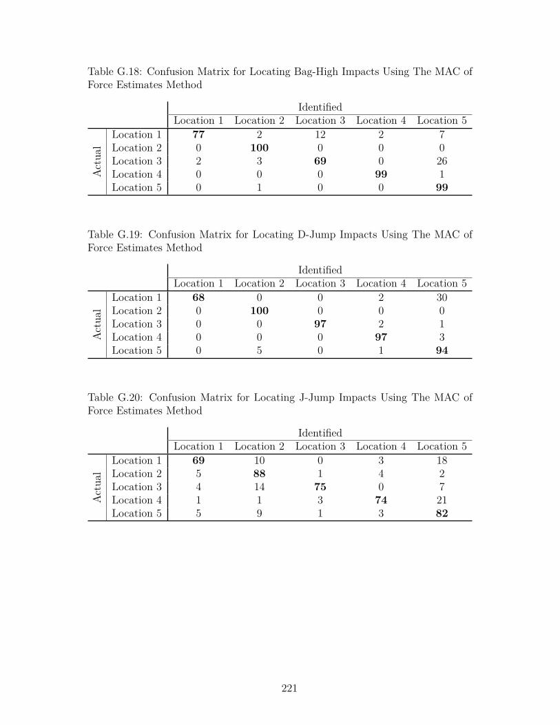
Table G.18: Confusion Matrix for Locating Bag-High Impacts Using The MAC ofForce Estimates Method
IdentifiedLocation 1 Location 2 Location 3 Location 4 Location 5
Act
ual
Location 1 77 2 12 2 7Location 2 0 100 0 0 0Location 3 2 3 69 0 26Location 4 0 0 0 99 1Location 5 0 1 0 0 99
Table G.19: Confusion Matrix for Locating D-Jump Impacts Using The MAC ofForce Estimates Method
IdentifiedLocation 1 Location 2 Location 3 Location 4 Location 5
Act
ual
Location 1 68 0 0 2 30Location 2 0 100 0 0 0Location 3 0 0 97 2 1Location 4 0 0 0 97 3Location 5 0 5 0 1 94
Table G.20: Confusion Matrix for Locating J-Jump Impacts Using The MAC ofForce Estimates Method
IdentifiedLocation 1 Location 2 Location 3 Location 4 Location 5
Act
ual
Location 1 69 10 0 3 18Location 2 5 88 1 4 2Location 3 4 14 75 0 7Location 4 1 1 3 74 21Location 5 5 9 1 3 82
221

Table G.21: Confusion Matrix for Locating W-Jump Impacts Using The MAC ofForce Estimates Method
IdentifiedLocation 1 Location 2 Location 3 Location 4 Location 5
Act
ual
Location 1 32 5 8 21 34Location 2 4 84 2 4 6Location 3 4 1 81 3 11Location 4 0 1 0 91 8Location 5 1 4 0 1 94
G.4 Time Shift Method
Time shifting looks at the location of peaks within the force estimates, and if the
peaks of the sensors align. The thought is that the location whose force estimates
have peaks that more closely align is where the impact occurred since the FEEL
Algorithm is time-independent. The standard deviation σ is taken of each point in
time τF̂i,jwhere the peak in the force estimate occurred as in Equation G.9 where i
is the location, and j is the sensor.
{Li} = σ
τF̂i,1
τF̂i,2...
τF̂i,j
(G.9)
The location of impact is consequently the location having the lowest standard
deviation value as this indicates the time in the force estimate the peaks occur are
more closely aligned as in Equation G.10.
L̂ = min({Li}) (G.10)
Results of this method are presented in the following confusion matrices.
222

Table G.22: Confusion Matrix for Locating Ball-Low Impacts Using The TimeShift Method
IdentifiedLocation 1 Location 2 Location 3 Location 4 Location 5
Act
ual
Location 1 100 0 0 0 0Location 2 0 99 0 0 1Location 3 0 0 100 0 0Location 4 0 0 0 100 0Location 5 0 0 0 0 100
Table G.23: Confusion Matrix for Locating Ball-High Impacts Using The TimeShift Method
IdentifiedLocation 1 Location 2 Location 3 Location 4 Location 5
Act
ual
Location 1 100 0 0 0 0Location 2 0 100 0 0 0Location 3 0 0 100 0 0Location 4 0 0 0 98 2Location 5 0 0 0 0 100
Table G.24: Confusion Matrix for Locating Bag-Low Impacts Using The Time ShiftMethod
IdentifiedLocation 1 Location 2 Location 3 Location 4 Location 5
Act
ual
Location 1 87 3 2 7 1Location 2 0 91 3 3 3Location 3 9 72 13 2 4Location 4 0 0 0 98 2Location 5 2 7 5 3 83
223

Table G.25: Confusion Matrix for Locating Bag-High Impacts Using The TimeShift Method
IdentifiedLocation 1 Location 2 Location 3 Location 4 Location 5
Act
ual
Location 1 81 10 1 4 4Location 2 0 99 0 0 1Location 3 16 62 20 1 1Location 4 1 2 1 94 2Location 5 6 9 12 4 69
Table G.26: Confusion Matrix for Locating D-Jump Impacts Using The Time ShiftMethod
IdentifiedLocation 1 Location 2 Location 3 Location 4 Location 5
Act
ual
Location 1 73 5 2 14 6Location 2 0 99 0 0 1Location 3 1 2 76 10 11Location 4 6 4 5 82 3Location 5 10 2 0 6 82
Table G.27: Confusion Matrix for Locating J-Jump Impacts Using The Time ShiftMethod
IdentifiedLocation 1 Location 2 Location 3 Location 4 Location 5
Act
ual
Location 1 81 1 8 3 7Location 2 11 75 4 7 3Location 3 20 7 55 14 4Location 4 1 0 3 86 10Location 5 29 3 24 16 28
224
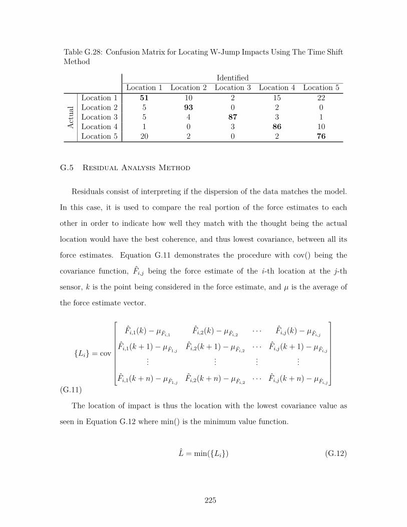
Table G.28: Confusion Matrix for Locating W-Jump Impacts Using The Time ShiftMethod
IdentifiedLocation 1 Location 2 Location 3 Location 4 Location 5
Act
ual
Location 1 51 10 2 15 22Location 2 5 93 0 2 0Location 3 5 4 87 3 1Location 4 1 0 3 86 10Location 5 20 2 0 2 76
G.5 Residual Analysis Method
Residuals consist of interpreting if the dispersion of the data matches the model.
In this case, it is used to compare the real portion of the force estimates to each
other in order to indicate how well they match with the thought being the actual
location would have the best coherence, and thus lowest covariance, between all its
force estimates. Equation G.11 demonstrates the procedure with cov() being the
covariance function, F̂i,j being the force estimate of the i-th location at the j-th
sensor, k is the point being considered in the force estimate, and µ is the average of
the force estimate vector.
{Li} = cov
F̂i,1(k) − µF̂i,1F̂i,2(k) − µF̂i,2
· · · F̂i,j(k) − µF̂i,j
F̂i,1(k + 1) − µF̂1,jF̂i,2(k + 1) − µF̂i,2
· · · F̂i,j(k + 1) − µF̂i,j
... ... ... ...
F̂i,1(k + n) − µF̂1,jF̂i,2(k + n) − µF̂i,2
· · · F̂i,j(k + n) − µF̂i,j
(G.11)
The location of impact is thus the location with the lowest covariance value as
seen in Equation G.12 where min() is the minimum value function.
L̂ = min({Li}) (G.12)
225

Table G.29: Confusion Matrix for Locating Ball-Low Impacts Using The ResidualAnalysis Method
IdentifiedLocation 1 Location 2 Location 3 Location 4 Location 5
Act
ual
Location 1 100 0 0 0 0Location 2 1 99 0 0 0Location 3 0 0 100 0 0Location 4 0 0 0 100 0Location 5 43 57 0 0 0
Table G.30: Confusion Matrix for Locating Ball-High Impacts Using The ResidualAnalysis Method
IdentifiedLocation 1 Location 2 Location 3 Location 4 Location 5
Act
ual
Location 1 100 0 0 0 0Location 2 0 100 0 0 0Location 3 0 1 99 0 0Location 4 0 0 0 100 0Location 5 13 87 0 0 0
Table G.31: Confusion Matrix for Locating Bag-Low Impacts Using The ResidualAnalysis Method
IdentifiedLocation 1 Location 2 Location 3 Location 4 Location 5
Act
ual
Location 1 93 0 0 7 0Location 2 13 87 0 0 0Location 3 93 1 6 0 0Location 4 13 4 0 83 0Location 5 57 43 0 0 0
226

Table G.32: Confusion Matrix for Locating Bag-High Impacts Using The ResidualAnalysis Method
IdentifiedLocation 1 Location 2 Location 3 Location 4 Location 5
Act
ual
Location 1 90 0 0 10 0Location 2 6 94 0 0 0Location 3 93 0 7 0 0Location 4 5 11 0 84 0Location 5 51 49 0 0 0
Table G.33: Confusion Matrix for Locating D-Jump Impacts Using The ResidualAnalysis Method
IdentifiedLocation 1 Location 2 Location 3 Location 4 Location 5
Act
ual
Location 1 96 0 0 4 0Location 2 44 46 0 10 0Location 3 69 0 17 14 0Location 4 4 0 0 96 0Location 5 53 45 0 2 0
Table G.34: Confusion Matrix for Locating J-Jump Impacts Using The ResidualAnalysis Method
IdentifiedLocation 1 Location 2 Location 3 Location 4 Location 5
Act
ual
Location 1 94 0 0 6 0Location 2 77 21 0 2 0Location 3 61 0 36 3 0Location 4 21 0 0 79 0Location 5 99 0 0 1 0
227
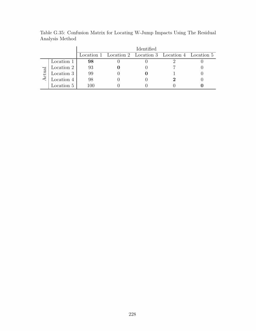
Table G.35: Confusion Matrix for Locating W-Jump Impacts Using The ResidualAnalysis Method
IdentifiedLocation 1 Location 2 Location 3 Location 4 Location 5
Act
ual
Location 1 98 0 0 2 0Location 2 93 0 0 7 0Location 3 99 0 0 1 0Location 4 98 0 0 2 0Location 5 100 0 0 0 0
228
Appendix H
Verification Experiments Additional Results
The following presents results from impacts that occurred on the remaining nodes
from the steel frame eight node trial in Section 5.4.2. Force estimates and force
correlations are presented for each case. FEEL Algorithm was successful in force and
location estimation in all cases.
229

H.1 Node 3 Impact
0.00 0.02 0.04 0.06 0.08 0.10Time (s)
−5
0
5
10
15
20Fo
rce
(N)
Sensor 1Sensor 2Sensor 3Actual
(a) F̂14,j
0.00 0.02 0.04 0.06 0.08 0.10Time (s)
−5
0
5
10
15
20
Forc
e(N
)
Sensor 1Sensor 2Sensor 3Actual
(b) F̂15,j
0.00 0.02 0.04 0.06 0.08 0.10Time (s)
−5
0
5
10
15
20
Forc
e(N
)
Sensor 1Sensor 2Sensor 3Actual
(c) F̂10,j
0.00 0.02 0.04 0.06 0.08 0.10Time (s)
−5
0
5
10
15
20Fo
rce
(N)
Sensor 1Sensor 2Sensor 3Actual
(d) F̂11,j
0.00 0.02 0.04 0.06 0.08 0.10Time (s)
−5
0
5
10
15
20
Forc
e(N
)
Sensor 1Sensor 2Sensor 3Actual
(e) F̂6,j
0.00 0.02 0.04 0.06 0.08 0.10Time (s)
−5
0
5
10
15
20
Forc
e(N
)
Sensor 1Sensor 2Sensor 3Actual
(f) F̂7,j
230
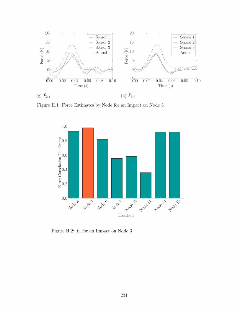
0.00 0.02 0.04 0.06 0.08 0.10Time (s)
−5
0
5
10
15
20
Forc
e(N
)Sensor 1Sensor 2Sensor 3Actual
(g) F̂2,j
0.00 0.02 0.04 0.06 0.08 0.10Time (s)
−5
0
5
10
15
20
Forc
e(N
)
Sensor 1Sensor 2Sensor 3Actual
(h) F̂3,j
Figure H.1: Force Estimates by Node for an Impact on Node 3
Node 2
Node 3
Node 6
Node 7
Node 10
Node 11
Node 14
Node 15
Location
0.0
0.2
0.4
0.6
0.8
1.0
Forc
eCo
rrela
tion
Coeffi
cient
Figure H.2: Li for an Impact on Node 3
231

H.2 Node 6 Impact
0.00 0.02 0.04 0.06 0.08 0.10Time (s)
−5
2
9
16
23
30Fo
rce
(N)
Sensor 1Sensor 2Sensor 3Actual
(a) F̂14,j
0.00 0.02 0.04 0.06 0.08 0.10Time (s)
−5
2
9
16
23
30
Forc
e(N
)
Sensor 1Sensor 2Sensor 3Actual
(b) F̂15,j
0.00 0.02 0.04 0.06 0.08 0.10Time (s)
−5
2
9
16
23
30
Forc
e(N
)
Sensor 1Sensor 2Sensor 3Actual
(c) F̂10,j
0.00 0.02 0.04 0.06 0.08 0.10Time (s)
−5
2
9
16
23
30Fo
rce
(N)
Sensor 1Sensor 2Sensor 3Actual
(d) F̂11,j
0.00 0.02 0.04 0.06 0.08 0.10Time (s)
−5
2
9
16
23
30
Forc
e(N
)
Sensor 1Sensor 2Sensor 3Actual
(e) F̂6,j
0.00 0.02 0.04 0.06 0.08 0.10Time (s)
−5
2
9
16
23
30
Forc
e(N
)
Sensor 1Sensor 2Sensor 3Actual
(f) F̂7,j
232

0.00 0.02 0.04 0.06 0.08 0.10Time (s)
−5
2
9
16
23
30
Forc
e(N
)Sensor 1Sensor 2Sensor 3Actual
(g) F̂2,j
0.00 0.02 0.04 0.06 0.08 0.10Time (s)
−5
2
9
16
23
30
Forc
e(N
)
Sensor 1Sensor 2Sensor 3Actual
(h) F̂3,j
Figure H.3: Force Estimates by Node for an Impact on Node 6
Node 2
Node 3
Node 6
Node 7
Node 10
Node 11
Node 14
Node 15
Location
0.0
0.2
0.4
0.6
0.8
1.0
Forc
eCo
rrela
tion
Coeffi
cient
Figure H.4: Li for an Impact on Node 6
233

H.3 Node 7 Impact
0.00 0.02 0.04 0.06 0.08 0.10Time (s)
0
20
40
60
80
Forc
e(N
)
Sensor 1Sensor 2Sensor 3Actual
(a) F̂14,j
0.00 0.02 0.04 0.06 0.08 0.10Time (s)
0
20
40
60
80
Forc
e(N
)
Sensor 1Sensor 2Sensor 3Actual
(b) F̂15,j
0.00 0.02 0.04 0.06 0.08 0.10Time (s)
0
20
40
60
80
Forc
e(N
)
Sensor 1Sensor 2Sensor 3Actual
(c) F̂10,j
0.00 0.02 0.04 0.06 0.08 0.10Time (s)
0
20
40
60
80Fo
rce
(N)
Sensor 1Sensor 2Sensor 3Actual
(d) F̂11,j
0.00 0.02 0.04 0.06 0.08 0.10Time (s)
0
20
40
60
80
Forc
e(N
)
Sensor 1Sensor 2Sensor 3Actual
(e) F̂6,j
0.00 0.02 0.04 0.06 0.08 0.10Time (s)
0
20
40
60
80
Forc
e(N
)
Sensor 1Sensor 2Sensor 3Actual
(f) F̂7,j
234

0.00 0.02 0.04 0.06 0.08 0.10Time (s)
0
20
40
60
80Fo
rce
(N)
Sensor 1Sensor 2Sensor 3Actual
(g) F̂2,j
0.00 0.02 0.04 0.06 0.08 0.10Time (s)
0
20
40
60
80
Forc
e(N
)
Sensor 1Sensor 2Sensor 3Actual
(h) F̂3,j
Figure H.5: Force Estimates by Node for an Impact on Node 7
Node 2
Node 3
Node 6
Node 7
Node 10
Node 11
Node 14
Node 15
Location
0.0
0.2
0.4
0.6
0.8
1.0
Forc
eCo
rrela
tion
Coeffi
cient
Figure H.6: Li for an Impact on Node 7
235
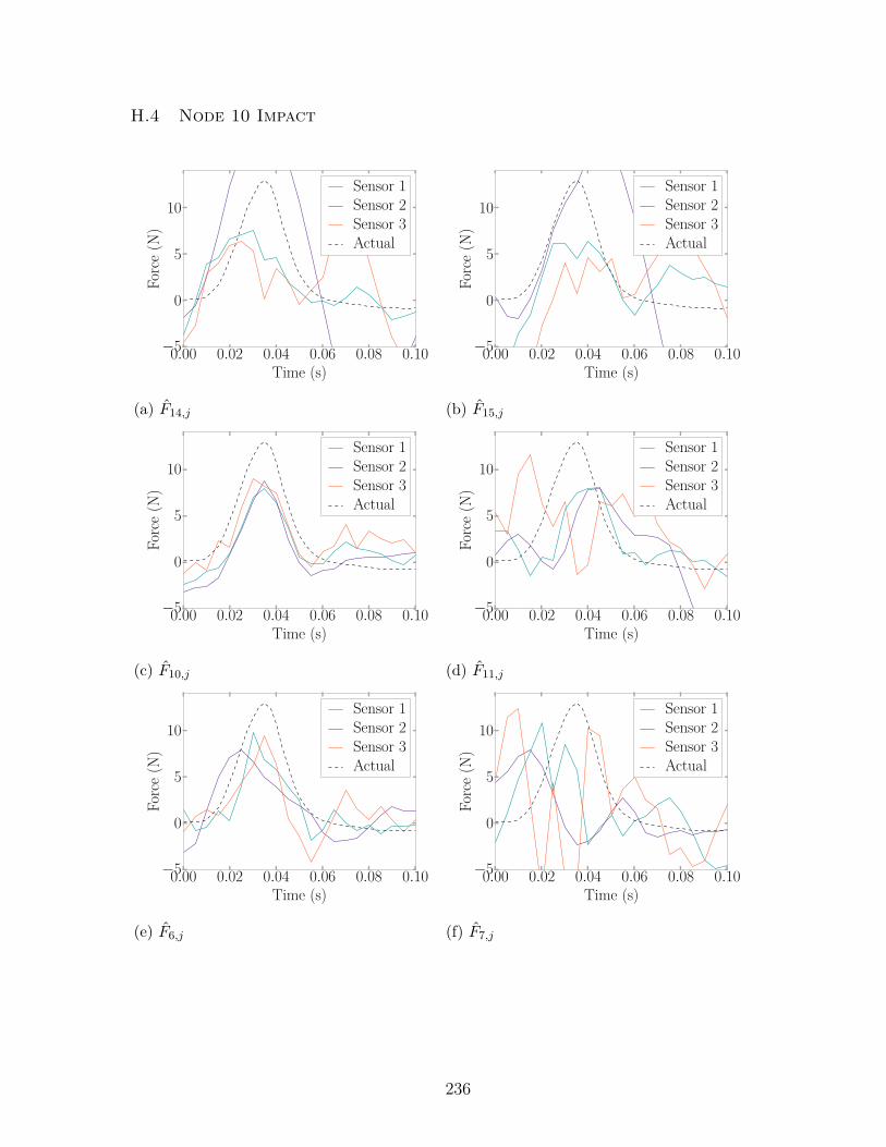
H.4 Node 10 Impact
0.00 0.02 0.04 0.06 0.08 0.10Time (s)
−5
0
5
10
Forc
e(N
)
Sensor 1Sensor 2Sensor 3Actual
(a) F̂14,j
0.00 0.02 0.04 0.06 0.08 0.10Time (s)
−5
0
5
10
Forc
e(N
)
Sensor 1Sensor 2Sensor 3Actual
(b) F̂15,j
0.00 0.02 0.04 0.06 0.08 0.10Time (s)
−5
0
5
10
Forc
e(N
)
Sensor 1Sensor 2Sensor 3Actual
(c) F̂10,j
0.00 0.02 0.04 0.06 0.08 0.10Time (s)
−5
0
5
10Fo
rce
(N)
Sensor 1Sensor 2Sensor 3Actual
(d) F̂11,j
0.00 0.02 0.04 0.06 0.08 0.10Time (s)
−5
0
5
10
Forc
e(N
)
Sensor 1Sensor 2Sensor 3Actual
(e) F̂6,j
0.00 0.02 0.04 0.06 0.08 0.10Time (s)
−5
0
5
10
Forc
e(N
)
Sensor 1Sensor 2Sensor 3Actual
(f) F̂7,j
236
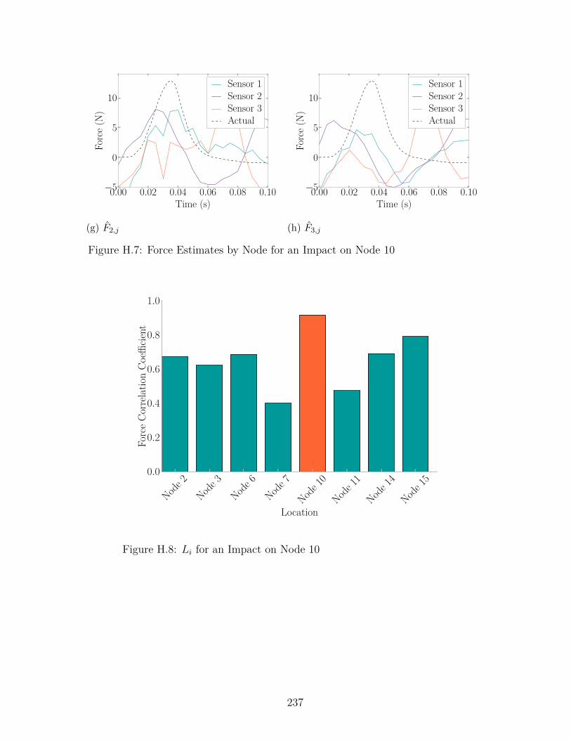
0.00 0.02 0.04 0.06 0.08 0.10Time (s)
−5
0
5
10Fo
rce
(N)
Sensor 1Sensor 2Sensor 3Actual
(g) F̂2,j
0.00 0.02 0.04 0.06 0.08 0.10Time (s)
−5
0
5
10
Forc
e(N
)
Sensor 1Sensor 2Sensor 3Actual
(h) F̂3,j
Figure H.7: Force Estimates by Node for an Impact on Node 10
Node 2
Node 3
Node 6
Node 7
Node 10
Node 11
Node 14
Node 15
Location
0.0
0.2
0.4
0.6
0.8
1.0
Forc
eCo
rrela
tion
Coeffi
cient
Figure H.8: Li for an Impact on Node 10
237
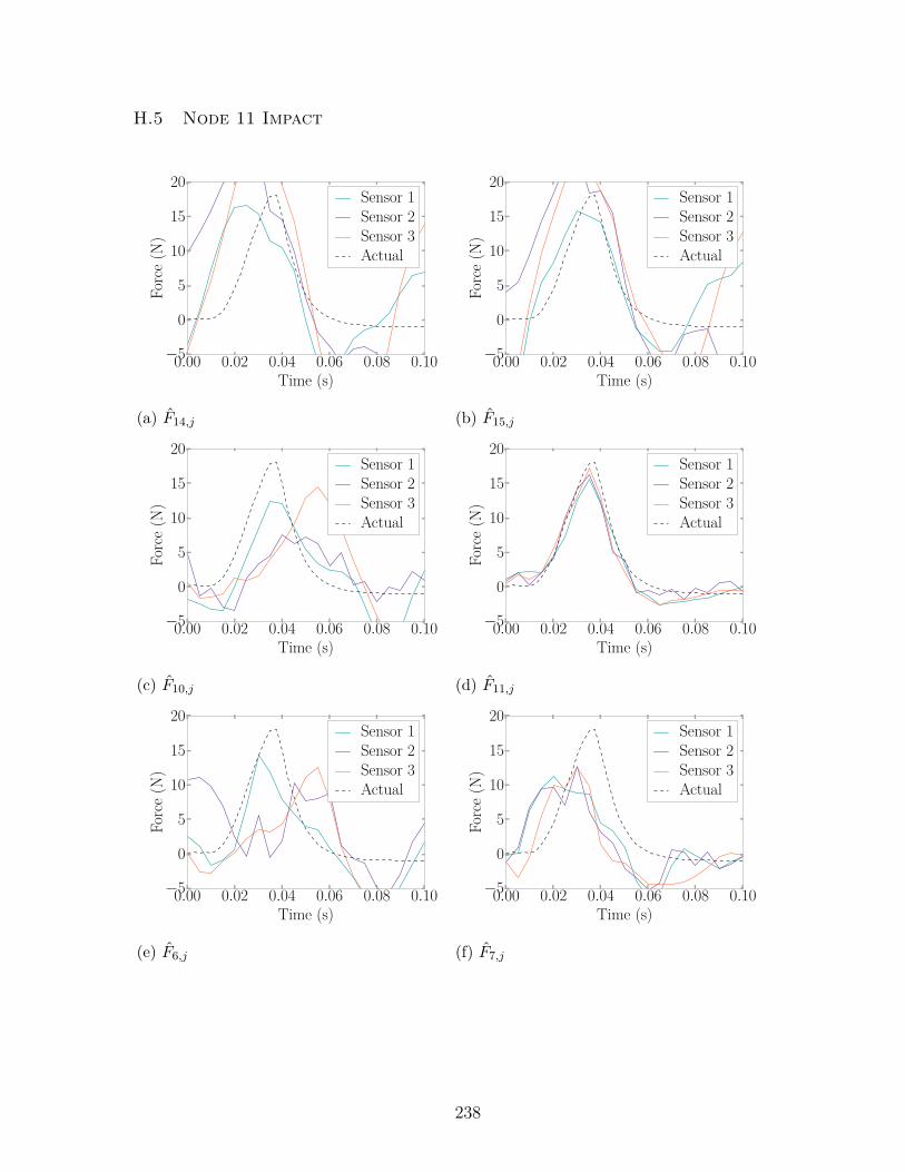
H.5 Node 11 Impact
0.00 0.02 0.04 0.06 0.08 0.10Time (s)
−5
0
5
10
15
20Fo
rce
(N)
Sensor 1Sensor 2Sensor 3Actual
(a) F̂14,j
0.00 0.02 0.04 0.06 0.08 0.10Time (s)
−5
0
5
10
15
20
Forc
e(N
)
Sensor 1Sensor 2Sensor 3Actual
(b) F̂15,j
0.00 0.02 0.04 0.06 0.08 0.10Time (s)
−5
0
5
10
15
20
Forc
e(N
)
Sensor 1Sensor 2Sensor 3Actual
(c) F̂10,j
0.00 0.02 0.04 0.06 0.08 0.10Time (s)
−5
0
5
10
15
20Fo
rce
(N)
Sensor 1Sensor 2Sensor 3Actual
(d) F̂11,j
0.00 0.02 0.04 0.06 0.08 0.10Time (s)
−5
0
5
10
15
20
Forc
e(N
)
Sensor 1Sensor 2Sensor 3Actual
(e) F̂6,j
0.00 0.02 0.04 0.06 0.08 0.10Time (s)
−5
0
5
10
15
20
Forc
e(N
)
Sensor 1Sensor 2Sensor 3Actual
(f) F̂7,j
238

0.00 0.02 0.04 0.06 0.08 0.10Time (s)
−5
0
5
10
15
20
Forc
e(N
)Sensor 1Sensor 2Sensor 3Actual
(g) F̂2,j
0.00 0.02 0.04 0.06 0.08 0.10Time (s)
−5
0
5
10
15
20
Forc
e(N
)
Sensor 1Sensor 2Sensor 3Actual
(h) F̂3,j
Figure H.9: Force Estimates by Node for an Impact on Node 11
Node 2
Node 3
Node 6
Node 7
Node 10
Node 11
Node 14
Node 15
Location
0.0
0.2
0.4
0.6
0.8
1.0
Forc
eCo
rrela
tion
Coeffi
cient
Figure H.10: Li for an Impact on Node 11
239

H.6 Node 14 Impact
0.00 0.02 0.04 0.06 0.08 0.10Time (s)
−5
0
5
10
15
20
25Fo
rce
(N)
Sensor 1Sensor 2Sensor 3Actual
(a) F̂14,j
0.00 0.02 0.04 0.06 0.08 0.10Time (s)
−5
0
5
10
15
20
25
Forc
e(N
)
Sensor 1Sensor 2Sensor 3Actual
(b) F̂15,j
0.00 0.02 0.04 0.06 0.08 0.10Time (s)
−5
0
5
10
15
20
25
Forc
e(N
)
Sensor 1Sensor 2Sensor 3Actual
(c) F̂10,j
0.00 0.02 0.04 0.06 0.08 0.10Time (s)
−5
0
5
10
15
20
25Fo
rce
(N)
Sensor 1Sensor 2Sensor 3Actual
(d) F̂11,j
0.00 0.02 0.04 0.06 0.08 0.10Time (s)
−5
0
5
10
15
20
25
Forc
e(N
)
Sensor 1Sensor 2Sensor 3Actual
(e) F̂6,j
0.00 0.02 0.04 0.06 0.08 0.10Time (s)
−5
0
5
10
15
20
25
Forc
e(N
)
Sensor 1Sensor 2Sensor 3Actual
(f) F̂7,j
240
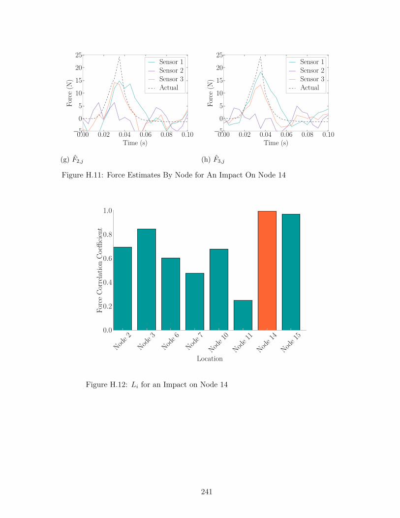
0.00 0.02 0.04 0.06 0.08 0.10Time (s)
−5
0
5
10
15
20
25
Forc
e(N
)Sensor 1Sensor 2Sensor 3Actual
(g) F̂2,j
0.00 0.02 0.04 0.06 0.08 0.10Time (s)
−5
0
5
10
15
20
25
Forc
e(N
)
Sensor 1Sensor 2Sensor 3Actual
(h) F̂3,j
Figure H.11: Force Estimates By Node for An Impact On Node 14
Node 2
Node 3
Node 6
Node 7
Node 10
Node 11
Node 14
Node 15
Location
0.0
0.2
0.4
0.6
0.8
1.0
Forc
eCo
rrela
tion
Coeffi
cient
Figure H.12: Li for an Impact on Node 14
241

H.7 Node 15 Impact
0.00 0.02 0.04 0.06 0.08 0.10Time (s)
0
10
20
30
40
Forc
e(N
)
Sensor 1Sensor 2Sensor 3Actual
(a) F̂14,j
0.00 0.02 0.04 0.06 0.08 0.10Time (s)
0
10
20
30
40
Forc
e(N
)
Sensor 1Sensor 2Sensor 3Actual
(b) F̂15,j
0.00 0.02 0.04 0.06 0.08 0.10Time (s)
0
10
20
30
40
Forc
e(N
)
Sensor 1Sensor 2Sensor 3Actual
(c) F̂10,j
0.00 0.02 0.04 0.06 0.08 0.10Time (s)
0
10
20
30
40Fo
rce
(N)
Sensor 1Sensor 2Sensor 3Actual
(d) F̂11,j
0.00 0.02 0.04 0.06 0.08 0.10Time (s)
0
10
20
30
40
Forc
e(N
)
Sensor 1Sensor 2Sensor 3Actual
(e) F̂6,j
0.00 0.02 0.04 0.06 0.08 0.10Time (s)
0
10
20
30
40
Forc
e(N
)
Sensor 1Sensor 2Sensor 3Actual
(f) F̂7,j
242
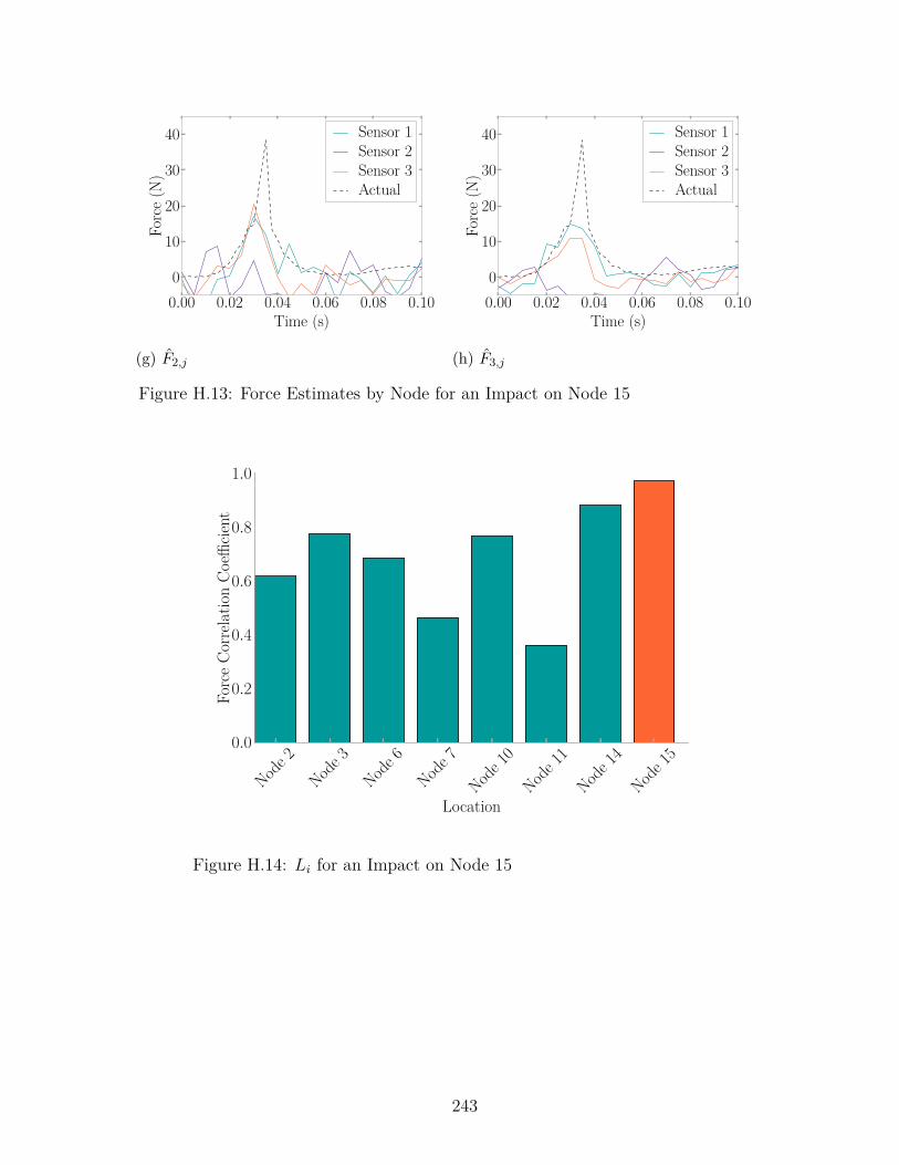
0.00 0.02 0.04 0.06 0.08 0.10Time (s)
0
10
20
30
40Fo
rce
(N)
Sensor 1Sensor 2Sensor 3Actual
(g) F̂2,j
0.00 0.02 0.04 0.06 0.08 0.10Time (s)
0
10
20
30
40
Forc
e(N
)
Sensor 1Sensor 2Sensor 3Actual
(h) F̂3,j
Figure H.13: Force Estimates by Node for an Impact on Node 15
Node 2
Node 3
Node 6
Node 7
Node 10
Node 11
Node 14
Node 15
Location
0.0
0.2
0.4
0.6
0.8
1.0
Forc
eCo
rrela
tion
Coeffi
cient
Figure H.14: Li for an Impact on Node 15
243

Appendix I
Implementation Experiment Force Hammer
Trial Additional Results
The following presents results from impacts that occurred on the remaining loca-
tions in the force hammer trial of the implementation experiments in Section 5.5.1.
Force estimates and force correlations are presented for each case. The FEEL Algo-
rithm was successful in force and location estimation in all cases.
244

I.1 Location 2 Impact
0.00 0.02 0.03 0.05 0.06Time (s)
−500
250
1000
1750
2500Fo
rce
(N)
Sensor 1Sensor 2Sensor 3Sensor 4Actual
(a) F̂1,j
0.00 0.02 0.03 0.05 0.06Time (s)
−500
250
1000
1750
2500
Forc
e(N
)
Sensor 1Sensor 2Sensor 3Sensor 4Actual
(b) F̂2,j
0.00 0.02 0.03 0.05 0.06Time (s)
−500
250
1000
1750
2500
Forc
e(N
)
Sensor 1Sensor 2Sensor 3Sensor 4Actual
(c) F̂3,j
0.00 0.02 0.03 0.05 0.06Time (s)
−500
250
1000
1750
2500
Forc
e(N
)Sensor 1Sensor 2Sensor 3Sensor 4Actual
(d) F̂4,j
0.00 0.02 0.03 0.05 0.06Time (s)
−500
250
1000
1750
2500
Forc
e(N
)
Sensor 1Sensor 2Sensor 3Sensor 4Actual
(e) F̂5,j
Figure I.1: Hammer Impact Force Estimations for an Impact on Location 2
245

Locat
ion1
Locat
ion2
Locat
ion3
Locat
ion4
Locat
ion5
0.0
0.2
0.4
0.6
0.8
1.0
Forc
eCo
rrela
tion
Coeffi
cient
Figure I.2: Hammer Impact Li for an Impact on Location 2
0.0 0.5 1.0 1.5 2.0Time (s)
−0.3
−0.2
−0.1
0.0
0.1
0.2
0.3
Acce
lerat
ion
(g)
Sensor 1Sensor 2Sensor 3Sensor 4
Figure I.3: Hammer on Location 2 Accelerations
246

I.2 Location 3 Impact
0.00 0.02 0.03 0.05 0.06Time (s)
−500
500
1500
2500
3500Fo
rce
(N)
Sensor 1Sensor 2Sensor 3Sensor 4Actual
(a) F̂1,j
0.00 0.02 0.03 0.05 0.06Time (s)
−500
500
1500
2500
3500
Forc
e(N
)
Sensor 1Sensor 2Sensor 3Sensor 4Actual
(b) F̂2,j
0.00 0.02 0.03 0.05 0.06Time (s)
−500
500
1500
2500
3500
Forc
e(N
)
Sensor 1Sensor 2Sensor 3Sensor 4Actual
(c) F̂3,j
0.00 0.02 0.03 0.05 0.06Time (s)
−500
500
1500
2500
3500
Forc
e(N
)Sensor 1Sensor 2Sensor 3Sensor 4Actual
(d) F̂4,j
0.00 0.02 0.03 0.05 0.06Time (s)
−500
500
1500
2500
3500
Forc
e(N
)
Sensor 1Sensor 2Sensor 3Sensor 4Actual
(e) F̂5,j
Figure I.4: Hammer Impact Force Estimations for an Impact on Location 3
247
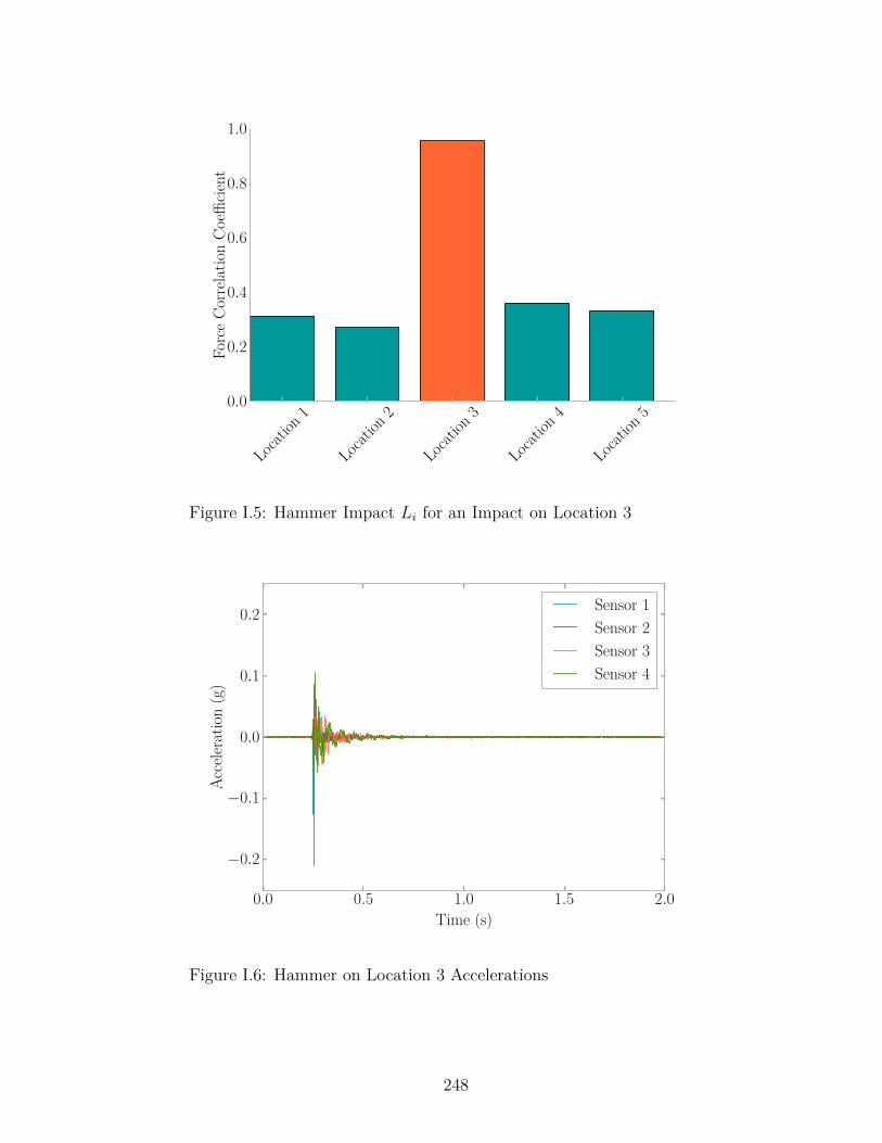
Locat
ion1
Locat
ion2
Locat
ion3
Locat
ion4
Locat
ion5
0.0
0.2
0.4
0.6
0.8
1.0
Forc
eCo
rrela
tion
Coeffi
cient
Figure I.5: Hammer Impact Li for an Impact on Location 3
0.0 0.5 1.0 1.5 2.0Time (s)
−0.2
−0.1
0.0
0.1
0.2
Acce
lerat
ion
(g)
Sensor 1Sensor 2Sensor 3Sensor 4
Figure I.6: Hammer on Location 3 Accelerations
248

I.3 Location 4 Impact
0.00 0.02 0.03 0.05 0.06Time (s)
−500
500
1500
2500
3500Fo
rce
(N)
Sensor 1Sensor 2Sensor 3Sensor 4Actual
(a) F̂1,j
0.00 0.02 0.03 0.05 0.06Time (s)
−500
500
1500
2500
3500
Forc
e(N
)
Sensor 1Sensor 2Sensor 3Sensor 4Actual
(b) F̂2,j
0.00 0.02 0.03 0.05 0.06Time (s)
−500
500
1500
2500
3500
Forc
e(N
)
Sensor 1Sensor 2Sensor 3Sensor 4Actual
(c) F̂3,j
0.00 0.02 0.03 0.05 0.06Time (s)
−500
500
1500
2500
3500
Forc
e(N
)Sensor 1Sensor 2Sensor 3Sensor 4Actual
(d) F̂4,j
0.00 0.02 0.03 0.05 0.06Time (s)
−500
500
1500
2500
3500
Forc
e(N
)
Sensor 1Sensor 2Sensor 3Sensor 4Actual
(e) F̂5,j
Figure I.7: Hammer Impact Force Estimations for an Impact on Location 4
249
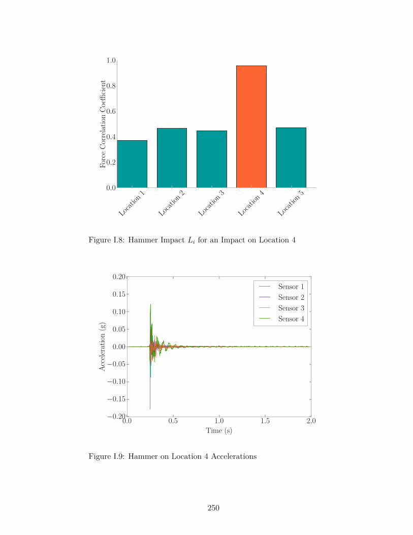
Locat
ion1
Locat
ion2
Locat
ion3
Locat
ion4
Locat
ion5
0.0
0.2
0.4
0.6
0.8
1.0
Forc
eCo
rrela
tion
Coeffi
cient
Figure I.8: Hammer Impact Li for an Impact on Location 4
0.0 0.5 1.0 1.5 2.0Time (s)
−0.20
−0.15
−0.10
−0.05
0.00
0.05
0.10
0.15
0.20
Acce
lerat
ion
(g)
Sensor 1Sensor 2Sensor 3Sensor 4
Figure I.9: Hammer on Location 4 Accelerations
250

I.4 Location 5 Impact
0.00 0.02 0.03 0.05 0.06Time (s)
−1000
750
2500
4250
6000Fo
rce
(N)
Sensor 1Sensor 2Sensor 3Sensor 4Actual
(a) F̂1,j
0.00 0.02 0.03 0.05 0.06Time (s)
−1000
750
2500
4250
6000
Forc
e(N
)
Sensor 1Sensor 2Sensor 3Sensor 4Actual
(b) F̂2,j
0.00 0.02 0.03 0.05 0.06Time (s)
−1000
750
2500
4250
6000
Forc
e(N
)
Sensor 1Sensor 2Sensor 3Sensor 4Actual
(c) F̂3,j
0.00 0.02 0.03 0.05 0.06Time (s)
−1000
750
2500
4250
6000
Forc
e(N
)Sensor 1Sensor 2Sensor 3Sensor 4Actual
(d) F̂4,j
0.00 0.02 0.03 0.05 0.06Time (s)
−1000
750
2500
4250
6000
Forc
e(N
)
Sensor 1Sensor 2Sensor 3Sensor 4Actual
(e) F̂5,j
Figure I.10: Hammer Impact Force Estimations for an Impact on Location 5
251

Locat
ion1
Locat
ion2
Locat
ion3
Locat
ion4
Locat
ion5
0.0
0.2
0.4
0.6
0.8
1.0
Forc
eCo
rrela
tion
Coeffi
cient
Figure I.11: Hammer Impact Li for an Impact on Location 5
0.0 0.5 1.0 1.5 2.0Time (s)
−0.4
−0.2
0.0
0.2
0.4
Acce
lerat
ion
(g)
Sensor 1Sensor 2Sensor 3Sensor 4
Figure I.12: Hammer on Location 5 Accelerations
252
Appendix J
EFFECT Active Learning Module Frequency
Domain Handout
This section contains a handout used in the EFFECT active learning module
discussed in Chapter 6.
253

EFFECT: Introduction to Frequency Domain by: Benjamin T. Davis, EIT
What is frequency domain?
“Put simply, a time-domain graph shows how a signal changes over time, whereas a frequency-
domain graph shows how much of the signal lies within each given frequency band over a range
of frequencies” [1].
You may have heard of the Fourier Series and its use in representing periodic signals through a summation
of cosine and sine terms. As a reminder, Equation 1 presents the Fourier Series [2].
S(t) = a0 +
∞∑j=1
aj cos (jω0t) +
∞∑j=1
bj sin (jω0t) (1)
This series is fundamental in creating a function for a periodic signal allowing for further analysis and
modeling. Taking a closer look at the series, one can see the theory that signals contain many sinusoidals of
varying amplitudes and frequencies. The larger the amplitude, the greater power that particular waveform
contributes to overall signal. This concept is what the frequency domain representation of a signal emulates
- frequencies present within a signal and how much each frequency contributes to the signal as a whole.
As an example, let’s take a sinusoidal loading that has a frequency of 10Hz and an amplitude of 20N. In
the time domain, this looks like a typical sine wave that has ten cycles in a second as in Figure 1a; however,
in the frequency domain (see Figure 1b) the frequency present in the signal, 10Hz, will create a peak as it
is rate with a large contribution (i.e. highest power).
0.0 0.2 0.4 0.6 0.8 1.0
Time (s)
−20
−10
0
10
20
Force
(N)
(a) Time Domain
0 20 40 60 80 100
Frequency (Hz)
0
50
100
150
200
250
300
350
Amplitude
(b) Frequency Domain
Figure 1: Signal Representations
University of South Carolina, Columbia Page 1 of 5
254
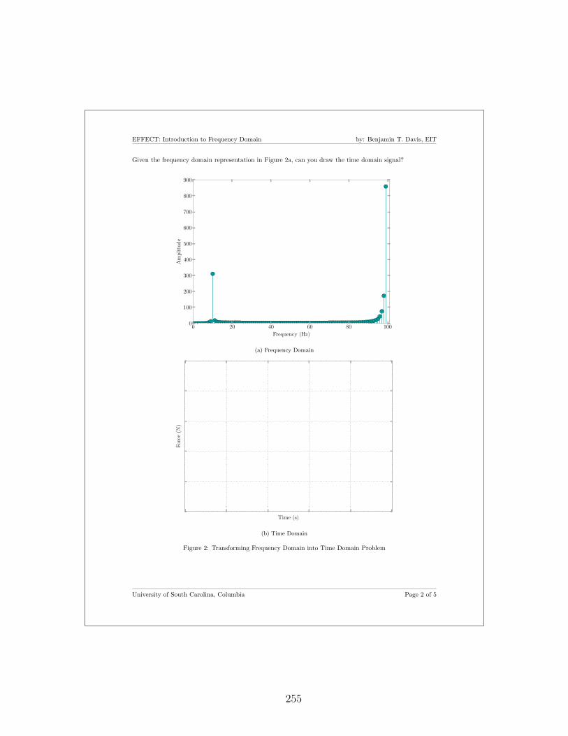
EFFECT: Introduction to Frequency Domain by: Benjamin T. Davis, EIT
Given the frequency domain representation in Figure 2a, can you draw the time domain signal?
0 20 40 60 80 100
Frequency (Hz)
0
100
200
300
400
500
600
700
800
900Amplitude
(a) Frequency Domain
Time (s)
Force
(N)
(b) Time Domain
Figure 2: Transforming Frequency Domain into Time Domain Problem
University of South Carolina, Columbia Page 2 of 5
255

EFFECT: Introduction to Frequency Domain by: Benjamin T. Davis, EIT
How to transform a time domain signal to frequency domain?
The Fourier Transform “is a generalization of the complex Fourier Series” [3] that enables the decomposition
of a periodic signal into its frequency components, or, in other words, “takes a time-based pattern, measures
every possible cycle, and returns the overall ‘cycle recipe’ (the strength, offset, and rotation speed for every
cycle that was found)” [4]. One can liken the concept to listening to an orchestra. The orchestra combines
multiple waveforms from the many instruments that make up its whole into one audio signal. Now, if you
were to focus in on an individual instrument within the orchestra, you would be focusing on one audio
signal. This is essentially what the Fourier Transform does. It breaks down the orchestra into individual
instruments each having their own frequency to create the frequency domain representation of the entire
orchestra’s sound. Equation 2 presents the Fourier Transform [3, 5]
F (ξ) =
∫ ∞
−∞S(t)e2πiξtdt (2)
where
ξ = frequency, Hz
S(t) = signal being evaluated with respect to time t
t = time, s
How to handle transforming more complex signals into the fre-
quency domain?
That first example wasn’t so rough, right? What if you had to decompose the signal in Figure 3a? A lot
more difficult to do by hand.
0.0 0.2 0.4 0.6 0.8 1.0
Time (s)
−60
−40
−20
0
20
40
60
Force
(N)
(a) Time Domain
0 20 40 60 80 100
Frequency (Hz)
0
20
40
60
80
100
120
140
160
180
Pow
er(dB)
(b) Frequency Domain
Figure 3: Complex Signal Example
Enter the Fast Fourier Transform (FFT) for machine calculations created by James Cooley and John Tukey
to make the transformation from time domain to frequency domain simple to do by computer [6]. Equation 3
presents the FFT [4, 6]
University of South Carolina, Columbia Page 3 of 5
256

EFFECT: Introduction to Frequency Domain by: Benjamin T. Davis, EIT
F (ξ) =
N−1∑n=0
S(n)e2πiξ(n/N) (3)
where
ξ = frequency, Hz
S(n) = signal being evaluated with respect to point n
n = data point
N = total number of data points
Fortunately for us, a lot of programming languages come with FFT built in. Take a look at the numpy
package available in Python in Code Snippet 1. Pretty easy, right?
1 import numpy as np
2
3 N = 200 # number of points in signal
4 dt = 1.0 / N # the time step between each data point of signal for one cycle
5
6 x = np.linspace(0, 2*np.pi, N) # in radians as np.sin() works in radians only
7 signal = 20*np.sin(10*x) + 50*np.sin(50*x) # the values of your signal
8 time = np.arange(0, len(signal)/dt, dt) # the time vector of the signal
9
10 sp = np.fft.fft(signal, len(signal)) # calculate the FFT for the discrete signal
11 freq = np.fft.fftfreq(time.shape[-1], dt) # grab the frequencies FFT evaluated
Code Snippet 1: Example of FFT Using Python Package NumPy
Using the code above on the complex signal in Figure 3a transforms the signal in the frequency domain
seen in Figure 3b. Notice how there is a peak at both 10Hz and 50Hz and that directly comes from the
frequencies in the sine functions used to create the signal. Additionally, pay attention to the decibel values
of the peaks. How does this relate to the amplitudes of each sine term that composes the signal?
University of South Carolina, Columbia Page 4 of 5
257
EFFECT: Introduction to Frequency Domain by: Benjamin T. Davis, EIT
References
[1] Frequency Domain. English. Wikipedia. 2015. url: https://en.wikipedia.org/wiki/Frequency domain.
[2] Anil K. Chopra. Dynamics of Structures: Theory and Applications to Earthquake Engineering. 4th ed.
Prentice Hall, 2011.
[3] Fourier Transform. English. Wolfram Math World. 2016. url: http : / /mathworld . wolfram . com /
FourierTransform.html.
[4] Kalid Azad. An Interactive Guide to the Fourier Transform. English. Better Explained. 2013. url:
http://betterexplained.com/articles/an-interactive-guide-to-the-fourier-transform/.
[5] Fourier Transform. English. Wikipedia. 2016. url: https://en.wikipedia.org/wiki/Fourier transform.
[6] James W. Cooley and John W. Tukey. “An Algorithm for the Machine Calculation of Complex Fourier
Series”. In: Mathematics of Computation 19.90 (1965), pp. 297–301. url: http://www.jstor.org/stable/
2003354?seq=1#page scan tab contents.
University of South Carolina, Columbia Page 5 of 5
258

Appendix K
EFFECT Active Learning Module Survey
This section contains the survey given to evaluate the EFFECT active learning
module discussed in Chapter 6.
259

ECIV 524 Structural Vibrations Survey
This is an anonymous survey, so do not write or sign your name. Please answer the followingquestions honestly.
1. What is your expected grade in this class? 2 A 2 B 2 C 2 D 2 F
2. What have you learned in this class?
3. Indicate how conducive to learning the following course activities were.
a. Lectures not conducive 2—2—2—2—2 conducive
b. In-Class Homework not conducive 2—2—2—2—2 conducive
c. Experiments and Lab Visits not conducive 2—2—2—2—2 conducive
d. Project not conducive 2—2—2—2—2 conducive
4. How confident do you feel about the following topics?
a. SDOF Free Vibration not confident 2—2—2—2—2 confident
b. SDOF Harmonic Excitation not confident 2—2—2—2—2 confident
c. SDOF Periodic Excitation not confident 2—2—2—2—2 confident
d. SDOF Impulse Excitation not confident 2—2—2—2—2 confident
e. SDOF Arbitrary Excitation not confident 2—2—2—2—2 confident
f. Applying the Central Difference Method not confident 2—2—2—2—2 confident
g. Frequency Domain Signal Representation not confident 2—2—2—2—2 confident
University of South Carolina 1 of 2
260

ECIV 524 Structural Vibrations Survey
5. What did you learn during the lab visit?
6a. Did the lab visit make the connection between math and physics easier tounderstand? 2 Yes 2 No
6b. How or why?
7. How would you improve the activities during the lab visit?
University of South Carolina 2 of 2
261

Appendix L
EFFECT Survey Responses
The following are responses given by students to the survey in Appendix K to
evaluate the EFFECT active learning module in Chapter 6. The check boxes for
questions three and four were given numeric values where one is not conducive/con-
fident and five is conducive/confident.
262

L.1 Student A
1. B
2. Structures have a natural frequency and will undergo damping. There aredifferent types of excitations that can be applied to a structure and each onewill have a different impact on the structure’s properties.
3. a) 5b) 4c) 3d) 4
4. a) 5b) 5c) 4d) 2e) 2f) 3g) 3
5. A structure can have more than one natural frequency, and when these areexcited you see peaks on the frequency vs. amplitude graph. A structure canonly have so much power done on it before it will break (max amplitude).
6. a) Yesb) Seeing the data graphically after an actual experiment helped relate the
concepts.
7. Some of the concepts were still pretty confusing, even after some explanation.Maybe give an overview of the basic concepts to keep in mind before doing theactual experiment.
263

L.2 Student B
1. A
2. We have learned a lot about the response of a SDoF to different forms of exci-tation including free vibrations, harmonic, impulse, and arbitrary. We studiedthe displacement, the velocity, and acceleration of the structures in question. Ialso learned how much this upper level class calls upon information we learnedin other classes. I liked that because it makes the effort in previous years feelworth it.
3. a) 5b) 2c) 4d) 3
4. a) 5b) 5c) 4d) 5e) 5f) 1g) 1
5. I was absent the day of the lab visit so I went on my own. I was able tomanipulate the structure myself by pushing on it and “felt” how strong it was.I was also able to observe the structure in vibration. Finally, we used a slowmotion camera and a ruler to determine displacement at certain time intervalswhich we used to calculate ζ.
6. a) Yesb) It helps to see the actual 3D structure in front of you. It gives you a mental
check while performing calculations. You know what the structure shoulddo so you can say your math would or would not match up with what youthink it should do.
7. Again, I wasn’t there but I feel if the entire class is struggling to calculatestiffness then the teacher should help us out. Our project was made moredifficult because we could not find k and neither could anyone else. Also, inclass homeworks are awful. Its basically a quiz because the teacher wouldnot answer any questions even if we were totally lost. Take home homeworkwe could bring to the teacher and ask for further explanation (teaching) of acertain topic.
264

L.3 Student C
1. A
2. I’ve learned about classifying systems and the process behind solving for thosesystems. We have gotten a chance to see how you would experimentally teststructures and how to take data from them.
3. a) 5b) 4c) 4d) 5
4. a) 5b) 5c) 4d) 5e) 4f) 3g) 3
5. I learned how to test a structure as well as saw how to graph and visualize labdata. From the last visit, I was able to see how a structure can be excited atall frequencies when struck by an impulse hammer.
6. a) Yesb) It helped to make the connection because the results nearly mimicked
the theoretical numbers and it confirmed that the physics was true andaccurately described structures.
7. The last lab was confusing dealing with frequency domain response mainlybecause I didn’t see David run through the simulations with the group thatwent to the lab. The theory helped solve the problem at the end, but I took aminute to grasp the physics behind exciting certain frequencies.
265

L.4 Student D
1. B
2. I have learned about different frequencies and how these frequencies come intoplay when trying to find the displacement, velocity, and acceleration of differ-ent structures. Also, how different types of excitations effect the structuresdifferently from each other.
3. a) 5b) 2c) 4d) 4
4. a) 5b) 4c) 2d) 5e) 5f) 3g) 2
5. I learned that without using time in the graphs, it was easier to see how muchand how little the different frequencies were.
6. a) Yesb) To perform an actual test and see the results was helpful. On the other
hand the results from the real world simulation aren’t perfect graphs whichis what the book usually deals with.
7. I’m sure there is a way to improve, but I found them useful and engaging.
266

L.5 Student E
1. B (student reported B+ which was not an option; changed to B)
2. Learned about SDOF systems and the many excitations a system can have andthe effects of them.
3. a) 5b) 4c) 3d) 4
4. a) 4b) 5c) 2d) 5e) 5f) 3g) 1
5. Learned that superposition is only valid with a linear system.
6. a) Nob) Because I guess I had not been involved in the lab during the whole dura-
tion of the experiment. It’s kinda hard to go in and learn in an hour anda half.
7. Not really sure. However, the lab visits do have an extracurricular feel and Ifeel it adds to the course.
267

L.6 Student F
1. A
2. How to model a single degree of freedom vibration due to arbitrary excitations.
3. a) 5b) 5c) 5d) 5
4. a) 5b) 5c) 1d) 5e) 5f) 5g) 3
5. How a structure reacts to various frequencies. Natural frequencies can be foundwith a simple impulse hammer test.
6. a) Yesb) It allowed myself to physically see what was going on.
7. Allow more brainstorming among the entire class versus working in pairs.
268

L.7 Student G
1. C
2. I have learned what damping ratios are, a better understanding of degrees offreedom. I’ve learned these are different types of vibrations and most can becalculated.
3. a) 5b) 5c) 4d) 4
4. a) 5b) 5c) 1d) 3e) 3f) 4g) 1
5. I learned that even such a large structure moves when enough force is applied.I also learned the structure moves not only up and down, but left and rightslightly.
6. a) Yesb) We got to physically see the vibrating of the structure happen.
7. I cannot think of anything at the moment.
269

L.8 Student H
1. D
2. The concepts of vibrations in structures with single degrees of freedom. Thetools/methods to use to analyze structural vibrations and what counts as failure.
3. a) 5b) 5c) 5d) 5
4. a) 4b) 4c) 3d) 4e) 4f) 3g) 2
5. That there are other methods/data to analyze experiments with rather thanjust something with time domain.
6. a) Yesb) The actual observation of the experiment allowed a firm connection be-
tween the concept and the math.
7. Perhaps a different experiment included, maybe a small demonstration in excelon what was one can analyze the data to reach conclusions for the key variablesnecessary for the math equations.
270

L.9 Student I
1. B
2. Dynamics of Structures, SDOF, free vibrations through undamped structures,viscously damped, and coloumb damped. SDOF harmonic excitations on struc-tures. Arbitrary and impulse responses. The central difference method andFourier series (a little bit).
3. a) 5b) 5c) 5d) 4
4. a) 4b) 4c) 3d) 4e) 4f) 3g) 2
5. We learned about frequency-domain responses. Basically, the representation ofa response of a system through amplitudes and frequency.
6. a) Nob) I thought we didn’t have a lot of time to further discuss the subject.
7. Make it a two-three day lecture/lab visit so we have more time for questions/ex-amples.
271

Appendix M
SSH Database Utilities Documentation
This presents the documentation for the Python package for interacting with the
database presented in Chapter 3.
272

SSH Database Utilities DocumentationRelease 1.0.0
Benjamin T. Davis
May 04, 2016
273

CONTENTS
1 License 1
2 Activity Density 2
3 Data Dumper 5
4 Dispersion Ratio 8
5 Event 10
6 Event Processor 13
7 Events by Day 22
8 Max Amplitude 25
9 Metrics 29
10 Monitored Days 32
11 NaN Density 35
12 Record Categorizer 37
13 Signal Energy 39
14 Rate of Dispersion 41
15 Standard Deviation Wave 43
16 System Groups 45
17 Value Jump 46
18 VA Room Info 48
i
274

Python Module Index 53
ii
275

CHAPTER
ONE
LICENSE
Copyright (c) 2016 Benjamin T. Davis. All rights reserved.
Redistribution and use in source and binary forms, with or without modification, are permittedprovided that the following conditions are met:
1. Redistributions of source code must retain the above copyright notice, this list of conditions andthe following disclaimer.
2. Redistributions in binary form must reproduce the above copyright notice, this list of condi-tions and the following disclaimer in the documentation and/or other materials provided with thedistribution.
3. Neither the name of the copyright holder nor the names of its contributors may be used toendorse or promote products derived from this software without specific prior written permission.
THIS SOFTWARE IS PROVIDED BY THE COPYRIGHT HOLDERS AND CONTRIBUTORS“AS IS” AND ANY EXPRESS OR IMPLIED WARRANTIES, INCLUDING, BUT NOT LIM-ITED TO, THE IMPLIED WARRANTIES OF MERCHANTABILITY AND FITNESS FOR APARTICULAR PURPOSE ARE DISCLAIMED. IN NO EVENT SHALL THE COPYRIGHTHOLDER OR CONTRIBUTORS BE LIABLE FOR ANY DIRECT, INDIRECT, INCIDENTAL,SPECIAL, EXEMPLARY, OR CONSEQUENTIAL DAMAGES (INCLUDING, BUT NOT LIM-ITED TO, PROCUREMENT OF SUBSTITUTE GOODS OR SERVICES; LOSS OF USE, DATA,OR PROFITS; OR BUSINESS INTERRUPTION) HOWEVER CAUSED AND ON ANY THE-ORY OF LIABILITY, WHETHER IN CONTRACT, STRICT LIABILITY, OR TORT (INCLUD-ING NEGLIGENCE OR OTHERWISE) ARISING IN ANY WAY OUT OF THE USE OF THISSOFTWARE, EVEN IF ADVISED OF THE POSSIBILITY OF SUCH DAMAGE.
1
276

CHAPTER
TWO
ACTIVITY DENSITY
Authors: Benjamin T. Davis, NSF Graduate Research Fellow
Date: 2014 August 20
Activity density is a tool to show how activity and area is by compressing acceleration events intoan hour by week format. This allows the user to easily see patterns of activity and give the userand idea of how dense a time is for activity.
2
277

SSH Database Utilities Documentation, Release 1.0.0
activity_density.get(sys=’all’, start=‘2010-01-01’, end=None, mac=None)Collects the activity density data from the SSH Database for specified systems for the spec-ified dates and specified sensor macs
Parameters
• sys (str or list) – The system group as a string being either
– va : VA Hospital Systems
– ph : Palmetto Health Systems
– all : all available systems
or a custom list of strings with each string having the form SSH-##
• start (str or datetime | default = ‘2010-01-01’) – The starting date toconsider with form YYYY-MM-DD or YYYY-MM-DD HH:MM:SS
• end (str or datetime | default = ‘2010-01-01’) – The ending date to con-sider with form YYYY-MM-DD or YYYY-MM-DD HH:MM:SS
• mac (list | default = None) – The unique machine address of the sensor ifonly a specific sensors are requested. Otherwise all sensors correspond-ing to a specific date will be returned
Returns activity (list) – The activity density information with row being and en-try and columns having form [0]dayOfWeekNumber, [1]hour, [2]numberO-fEvents
Notes
•uses the ‘accel_events’ table
•adapted from SSH Data analysis/Database_utils_py/ActivityDensity/
3
278

SSH Database Utilities Documentation, Release 1.0.0
activity_density.plot(activity)Plots the data received from activity_density.get() as a heatmap
Parameters activity (list) – The activity density information with row beingand entry and columns having form [0]dayOfWeekNumber, [1]hour, [2]num-berOfEvents
Returns axis (<matplotlib.axes.AxesSubplot>) – The handle for the plot axis
Notes
•The axis default to light gray in color
•Change various features of the plot using axis; e.g.
>>> pyplot.setp(axis.lines, color='r', linewidth=2.0, linestyle='-')
•adapted from SSH Data analysis/Database_utils_py/ActivityDensity/
4
279

CHAPTER
THREE
DATA DUMPER
Authors: Benjamin T. Davis, NSF Graduate Research Fellow
Date: 2016 April 07
Grabs the specified system group’s data and saves to a csv file.
5
280

SSH Database Utilities Documentation, Release 1.0.0
data_dumper.run(username, password, sys=’all’, tables=[’accel_events’, ‘sys-tem_log’, ‘downloads’, ‘events’], nrows=2000, savedir=’./’)
Dumps the database into a series of csv files, each file containing nrows of data
Parameters
• username (str) – The username having admin rights for the human ac-tivity database
• password (str) – The password for the username
• sys (list | default = ‘all’) – The system group as a string being either
– va : VA Hospital Systems
– ph : Palmetto Health Systems
– all : all available systems
or a custom list of strings with each string having the form SSH-##
• tables (list | default = [’accel_events’, ‘system_log’, ‘downloads’,‘events’]) – A list of table name strings that should be dumped
• nrows (int | default = 2000) – The number of rows to dump into the csvfile at a time; this prevents possible errors from server timeouts on largedatasets
• savedir (str | default = ‘./’) – The directory to save in csv files in; stringshould end with ‘/’
Notes
•Saves the csv files to the server housing the MySQL database based on the savedirdirectory
6
281

SSH Database Utilities Documentation, Release 1.0.0
data_dumper.make_system_options(systems)Makes the MySQL where clause for choosing selected systems
Parameters systems (list) – the system names
7
282

CHAPTER
FOUR
DISPERSION RATIO
Authors: Benjamin T. Davis, NSF Graduate Research Fellow
Date: 2015 March 24
8
283

SSH Database Utilities Documentation, Release 1.0.0
dispersion_ratio.calc(data, window=250, noverlap=249)Calculates the dispersion ratio which is defined as max(std_wave) / min(std_wave)
Parameters
• data (list) – data to perform the operation on (e.g. accelerometer data)
• window (int | default = 250) – the number of points to use per operation;must be less than len(data)
• noverlap (int | default = 249) – number of points to overlap per window;must be less than window
Returns dr (float) – the dispersion ratio
Notes
•performs calculation as if NaN was not present. Meaning that data=[1,2,3,NaN,4,5]and x=[0,1,2,3,4,5] would be treated as data=[1,2,3,4,5] and x=[0,1,2,4,5], respectively
•adapted from SSH Data Analysis/Database_utils_py/StandardDeviationSNR/
9
284

CHAPTER
FIVE
EVENT
Author: Benjamin T. Davis, NSF Graduate Research Fellow <[email protected]>
Date: 2015 July 2
10
285

SSH Database Utilities Documentation, Release 1.0.0
event.get(system, event_date, mac=None)Grabs an acceleration event from the SSH database
Parameters
• system (str) – The system that saw the event using the format SSH-##.Systems may be obtained from the sys_group module
• event_date (str or datetime) – The full string or datetime object of formYYYY-MM-DD HH:MM:SS
• mac (str | default = None) – The unique machine address of the sensor ifonly a specific sensor is requested. Otherwise all sensors correspondingto a specific date will be returned.
Returns event (list) – where each slot contains a sublist of the form[0]event_date, [1]sensor_mac, [2]vertical_axis, [3]accelerationData, [4]sys-tem, [5]system_activation
Notes
•uses the ‘accel_events’ table
•only returns one event at a time
•adapted from SSH Data analysis/Database_utils_py/AccelEventPlot/
11
286

SSH Database Utilities Documentation, Release 1.0.0
event.plot(event, fs=1, one_plot=False)Plots the event gathered by event.get()
Parameters
• event (list) – The list of event data features from event.get()
• fs (float | default = 1) – The sampling rate of the data in Hz
• one_plot (boolean | default = False) – If you want the data to be plottedin one window or each sensor to be plotted in its own window
Returns axis (list or <matplotlib.axes.AxesSubplot>) – If one_plot was set toTrue, this will be a list of <matplotlib.axes.AxesSubplot> objects, one foreach sensor’s plot. Otherwise this will be a single object
Notes
•The axis default to light gray in color
•Change various features of the plot using axis; e.g.
>>> pyplot.setp(axis.lines, color='r', linewidth=2.0, linestyle='-')
•adapted from SSH Data analysis/Database_utils_py/AccelEventPlot/
12
287

CHAPTER
SIX
EVENT PROCESSOR
Authors: Benjamin T. Davis, NSF Graduate Research Fellow
Date: 2016 February 09
The event processor works through records processes said records for the various metrics. Theresults are stored in the human-induced vibration activity database.
13
288

SSH Database Utilities Documentation, Release 1.0.0
event_processor.insert_or_update_parameter(cursor, system, event_date,mac, parameter, value)
Attempts to insert, or failing that update, the parameter value in the event_parameters table
Parameters
• cursor (pymysql.cursors.Cursor) – The pymysql cursor object for exe-cuting queries
• system (str) – The system relating to the parameter
• event_date (str or datetime) – The event date with form YYYY-MM-DDor YYYY-MM-DD HH:MM:SS
• mac (str) – The MAC address relating to this parameter
• parameter (str) – The parameter to insert or update
• value (str) – The value of the parameter
14
289

SSH Database Utilities Documentation, Release 1.0.0
event_processor.mark_event_parameter_processed(cursor, event_date,mac, parameter)
Marks an event’s parameter as processed in event_processing table
Parameters
• cursor (pymysql.cursors.Cursor) – The pymysql cursor object for exe-cuting queries
• event_date (str or datetime) – The event date with form YYYY-MM-DDor YYYY-MM-DD HH:MM:SS
• mac (str) – The MAC address relating to this parameter
• parameter (str) – The parameter to insert or update
Note:•Switching the value of ‘processed’ from 0 to 1 indicates the event has has been pro-cessed. In other words, 0 indicated unprocessed and 1 indicates processed.
15
290

SSH Database Utilities Documentation, Release 1.0.0
event_processor.all_records(metric=’ampmax’, start=‘2010-01-01’,end=None)
Generates processing information in the event_processing table for all acceleration recordsin accel_events for a date range
Parameters
• metric (str | default = ‘ampmax’) – The metric to process. Metrics aredefined in the parameters table
• start (str or datetime | default = ‘2010-01-01’) – The starting date toconsider with form YYYY-MM-DD or YYYY-MM-DD HH:MM:SS
• end (str or datetime | default = None) – The ending date to consider withform YYYY-MM-DD or YYYY-MM-DD HH:MM:SS
Note:•Ignores records saying ‘No Data’
16
291

SSH Database Utilities Documentation, Release 1.0.0
event_processor.all_records_category_svm(start=‘2010-01-01’,end=None)
Adds all records processing information to the event_processing table for generated theSVM-defined category
Parameters
• start (str or datetime | default = ‘2010-01-01’) – The starting date toconsider with form YYYY-MM-DD or YYYY-MM-DD HH:MM:SS
• end (str or datetime | default = None) – The ending date to consider withform YYYY-MM-DD or YYYY-MM-DD HH:MM:SS
Note:•Ignores records saying ‘No Data’
•Ignores records with ‘NaN’ present, i.e. incomplete records
•Ignores records with a MADr greater than 0.95 as these are considered sensor errors
•Ignores records that have already been categorized with category-manual as these areconsidered training records for the SVM
17
292

SSH Database Utilities Documentation, Release 1.0.0
event_processor.records_missing_metric(metric=’ampmax’, start=‘2010-01-01’, end=None)
Looks for records missing the specified metric in the events_parameters table and then gen-erates processing information in the event_processing table
Parameters
• metric (str | default = ‘ampmax’) – The metric to process. Metrics aredefined in the parameters table
• start (str or datetime | default = ‘2010-01-01’) – The starting date toconsider with form YYYY-MM-DD or YYYY-MM-DD HH:MM:SS
• end (str or datetime | default = None) – The ending date to consider withform YYYY-MM-DD or YYYY-MM-DD HH:MM:SS
Note:•Ignores records saying ‘No Data’
18
293

SSH Database Utilities Documentation, Release 1.0.0
event_processor.records_missing_category_svm(start=‘2010-01-01’,end=None)
Looks for records missing an SVM-defined category in the events_parameters table and thengenerates processing information in the event_processing table
Parameters
• start (str or datetime | default = ‘2010-01-01’) – The starting date toconsider with form YYYY-MM-DD or YYYY-MM-DD HH:MM:SS
• end (str or datetime | default = None) – The ending date to consider withform YYYY-MM-DD or YYYY-MM-DD HH:MM:SS
Note:•Ignores records saying ‘No Data’
•Ignores records with ‘NaN’ present, i.e. incomplete records
•Ignores records with a MADr greater than 0.95 as these are considered sensor errors
•Ignores records that have already been categorized with category-manual as these areconsidered training records for the SVM
19
294

SSH Database Utilities Documentation, Release 1.0.0
event_processor.generate_metric(metric=’ampmax’, fs=316.0, window=250,noverlap=249)
Generates the specified metric based on the table event_processing which is generated usingall_records() or records_missing_metric()
Parameters
• metric (str | default = ‘ampmax’) – The metric to process. Metrics aredefined in the parameters table
• fs (float | default = 316.0) – The sampling rate (Hz) of the records beingevaluated. This is set to 316 Hz which was shown by Benjamin T. Davisin his PhD dissertation to be the frequency of the Camp Hill sensor; usedfor senergy
• window (int | default = 250) – The number of points to use per operation;must be less than len(data); used for stdsnr
• noverlap (int | default = 249) – Number of points to overlap per window;must be less than window; used for stdsnr
20
295

SSH Database Utilities Documentation, Release 1.0.0
event_processor.svm_categorize()Categorizes records using a SVM from Benjamin T. Davis’s dissertation, Characterization ofHuman-Induced Vibrations, that learns based on category-manual. It operates using the tableevent_processing which is generated using records_missing_category_svm()
Note:•The SVM learns based on category-manual. The radial basis function kernel using theDisperion Ratio metric was found to be the best, and is what the SVM provided hereutilizes.
•if DR = infinity, category is marked as 0 for unsure. These are typically signals con-taining all the same values.
21
296

CHAPTER
SEVEN
EVENTS BY DAY
Authors: Benjamin T. Davis, NSF Graduate Research Fellow
Date: 2014 August 14
Events by day shows how many acceleration events occur on each month of each day which givesthe viewer an idea of how active an area is. This is a version of Activity Density.
22
297

SSH Database Utilities Documentation, Release 1.0.0
events_by_day.get(sys=’all’, start=‘2010-01-01’, end=None, mac=None)Collects the event data from the SSH Database specified systems for the specified dates andspecified sensor macs
Parameters
• sys (str or list) – The system group as a string being either
– va : VA Hospital Systems
– ph : Palmetto Health Systems
– all : all available systems
or a custom list of strings with each string having the form SSH-##
• start (str or datetime | default = ‘2010-01-01’) – The starting date toconsider with form YYYY-MM-DD or YYYY-MM-DD HH:MM:SS
• end (str or datetime | default = ‘2010-01-01’) – The ending date to con-sider with form YYYY-MM-DD or YYYY-MM-DD HH:MM:SS
• mac (list | default = None) – The unique machine address of the sensor ifonly a specific sensors are requested. Otherwise all sensors correspond-ing to a specific date will be returned
Returns events (list) – events by day with columns having the form [0]year,[1]month, [2]day, [3]event count, [4]month abbreviation
Notes
•uses the ‘accel_events’ table
•adapted from SSH Data analysis/Database_utils_py/EventsByDay/
23
298

SSH Database Utilities Documentation, Release 1.0.0
events_by_day.plot(events, logscale=False)Plots the data received from events_by_day.get() as a heatmap
Parameters
• events (list) – events by day with columns having the form [0]year,[1]month, [2]day, [3]event count, [4]month abbreviation
• logscale (boolean | default = False) – determines if output should be inlog scale
Returns axis (<matplotlib.axes.AxesSubplot>) – The handle for the plot axis
Notes
•The axis default to light gray in color
•Change various features of the plot using axis; e.g.
>>> pyplot.setp(axis.lines, color='r', linewidth=2.0, linestyle='-')
•adapted from SSH Data analysis/Database_utils_py/ActivityDensity/
24
299

CHAPTER
EIGHT
MAX AMPLITUDE
Authors: Benjamin T. Davis, NSF Graduate Research Fellow
Date: 2015 January 16
25
300

SSH Database Utilities Documentation, Release 1.0.0
max_amplitude.calc(data)Finds the maximum amplitude of the data determined by max(abs(data))
Parameters data (list) – data to perform the operation on (e.g. accelerometerdata)
Returns max_amplitude (float) – the maximum amplitude present in the data
26
301

SSH Database Utilities Documentation, Release 1.0.0
max_amplitude.difference(data)Finds the maximum amplitude difference (MAD) of the data which is the max change of theabsolute values of the descending sorted data
Parameters data (numpy.array) – data to perform the operation on (e.g. ac-celerometer data)
Returns mad (float) – the maximum amplitude difference present in the data
27
302
SSH Database Utilities Documentation, Release 1.0.0
max_amplitude.get(systemDate)Finds the maximum amplitudes of the events given based on metric2 in the SSH Database
Parameters systemDate (2D list) – a list with system names as the first columnand an event date as the second column
>>> systemDate = [[['SSH-36'], ['2013-04-25 16:48:03']],[['SSH-37'], ['2014-06-01 00:32:24']]]
Returns amplitudes (2D array) – an array containing the results for all the sys-tem and date combinations from systemDate with each row having the form[[0] system, [1] date, [2] mac, [3] amplitude]. The mac slot corresponds tothe mac of the sensor that has the maximum amplitude. The amplitude slotcontains the max amplitude value.
Notes
•adapted from SSH Data Analysis/Database_utils_py/maxAmplitude/
28
303

CHAPTER
NINE
METRICS
Authors: Benjamin T. Davis, NSF Graduate Research Fellow
Date: 2015 November 05
Metrics provides functions for grabbing signal metric information that is stored in the database.
29
304

SSH Database Utilities Documentation, Release 1.0.0
metrics.get(sys=’all’, start=‘2010-01-01’, end=None, param=’all’, mac=None)Collects the specified signal metrics
Parameters
• sys (str or list) – The system group as a string being either
– va : VA Hospital Systems
– ph : Palmetto Health Systems
– all : all available systems
or a custom list of strings with each string having the form SSH-##
• start (str or datetime | default = ‘2010-01-01’) – The starting date toconsider with form YYYY-MM-DD or YYYY-MM-DD HH:MM:SS
• end (str or datetime | default = ‘2010-01-01’) – The ending date to con-sider with form YYYY-MM-DD or YYYY-MM-DD HH:MM:SS
• param (list | default = ‘all’) – The name of the metrics in the databaseto retrieve or ‘all’ to grab everything
• mac (list | default = None) – The unique machine address of the sensor ifonly a specific sensors are requested. Otherwise all sensors correspond-ing to a specific date will be returned
Returns metrics (list) – The list of metrics requested where [0]system, [1]date[2]sensor mac, [3]param1 value, [4]param2 value,...
Notes
•uses the ‘event_parameters’ table
•uses the ‘parameters’ table
•adapted from SSH Data analysis/Database_utils_py/SignalMetricPlot/
30
305

SSH Database Utilities Documentation, Release 1.0.0
metrics.getGrouped(sys=’all’, start=‘2010-01-01’, end=None, param=’all’,mac=None)
Collects the specified signal metrics as a group. The grouping only returns records thatcontain the metrics listed after applying a filter to the values to ignore “NaN” and empty.
Parameters
• sys (str or list) – The system group as a string being either
– va : VA Hospital Systems
– ph : Palmetto Health Systems
– all : all available systems
or a custom list of strings with each string having the form SSH-##
• start (str or datetime | default = ‘2010-01-01’) – The starting date toconsider with form YYYY-MM-DD or YYYY-MM-DD HH:MM:SS
• end (str or datetime | default = ‘2010-01-01’) – The ending date to con-sider with form YYYY-MM-DD or YYYY-MM-DD HH:MM:SS
• param (list | default = ‘all’) – The name of the metrics in the databaseto retrieve or ‘all’ to grab everything
• mac (list | default = None) – The unique machine address of the sensor ifonly a specific sensors are requested. Otherwise all sensors correspond-ing to a specific date will be returned
Returns metrics (list) – The list of metrics requested where [0]system, [1]date[2]sensor mac, [3]param1 value, [4]param2 value,...
Notes
•uses the ‘event_parameters’ table
•uses the ‘parameters’ table
•adapted from SSH Data analysis/Database_utils_py/SignalMetricPlot/
31
306

CHAPTER
TEN
MONITORED DAYS
Authors: Benjamin T. Davis, NSF Graduate Research Fellow
Date: 2014 September 29
Monitored Days displays how many sensors were active by day. Gives user an idea of how well asystem and its sensors are operating.
32
307

SSH Database Utilities Documentation, Release 1.0.0
monitored_days.get(sys=’all’, start=‘2010-01-01’, end=None, mac=None)Collects the monitored day data from the SSH Database for specified systems for the speci-fied dates and specified sensor macs
Parameters
• sys (str or list) – The system group as a string being either
– va : VA Hospital Systems
– ph : Palmetto Health Systems
– all : all available systems
or a custom list of strings with each string having the form SSH-##
• start (str or datetime | default = ‘2010-01-01’) – The starting date toconsider with form YYYY-MM-DD or YYYY-MM-DD HH:MM:SS
• end (str or datetime | default = ‘2010-01-01’) – The ending date to con-sider with form YYYY-MM-DD or YYYY-MM-DD HH:MM:SS
• mac (list | default = None) – The unique machine address of the sensor ifonly a specific sensors are requested. Otherwise all sensors correspond-ing to a specific date will be returned
Returns sensors_active (list) – The monitored day information with row beingand entry and columns having form [0]day, [1]month, [2]year, [3]numberOf-Sensors, [4]monthName
Notes
•uses the ‘system_log’ table
•adapted from SSH Data Analysis/Database_utils_py/MonitoredDays/
33
308

SSH Database Utilities Documentation, Release 1.0.0
monitored_days.plot(sensors_active)Plots the data received from monitored_days.get() as a heatmap
Parameters sensors_active (list) – The monitored day information with row be-ing and entry and columns having form [0]day, [1]month, [2]year, [3]num-berOfSensors, [4]monthName
Returns axis (<matplotlib.axes.AxesSubplot>) – The handle for the plot axis
Notes
•The axis default to light gray in color
•Change various features of the plot using axis; e.g.
>>> pyplot.setp(axis.lines, color='r', linewidth=2.0, linestyle='-')
•adapted from SSH Data Analysis/Database_utils_py/MonitoredDays/
34
309

CHAPTER
ELEVEN
NAN DENSITY
Authors: Benjamin T. Davis, NSF Graduate Research Fellow
Date: 2015 March 20
35
310

SSH Database Utilities Documentation, Release 1.0.0
nan_density.calc(data)Calculates the density of nan values in a data set. The equation is # nan / total points
Parameters data (list) – data to perform the operation on (e.g. accelerometerdata)
Returns density (float) – the density of NaN in the data
Notes
•adapted from SSH Data Analysis/Database_utils_py/nanDensity/
36
311

CHAPTER
TWELVE
RECORD CATEGORIZER
Authors: Benjamin T. Davis, NSF Graduate Research Fellow
Date: 2015 March 26
Browses falls database at random and allows user to categorize the signal
37
312

SSH Database Utilities Documentation, Release 1.0.0
record_categorize.run()Runs the categorizer and guides the user through the process while saving the user’s re-sponses to the database in table event_parameters with the parameter name being category-manual
Notes
•uses the ‘accel_events’ table
•adapted from SSH Data analysis/Database_utils_py/manualRecordCategorizer/
38
313

CHAPTER
THIRTEEN
SIGNAL ENERGY
Authors: Benjamin T. Davis, NSF Graduate Research Fellow
Date: 2015 April 02
39
314

SSH Database Utilities Documentation, Release 1.0.0
signal_energy.calc(y, x=None, dx=1.0)Determines the signal energy (signal processing version). This is defined to be inte-gral(data^2).The integration scheme used here is the trapezoidal rule.
Parameters
• y (list) – the y values of the signal
• x (list | default = None) – the x coordinates corresponding to data
• dx (float | default = 1.0) – the spacing between elements of data; if x isnot specified, dx is used
Returns senergy (float) – the signal energy
Notes
•https://en.wikipedia.org/wiki/Energy_(signal_processing)
•performs integration as if NaN was not present. Meaning that data=[1,2,3,NaN,4,5]and x=[0,1,2,3,4,5] would be treated as data=[1,2,3,4,5] and x=[0,1,2,4,5], respectively
•adapted from SSH Data Analysis/Database_utils_py/signalEnergy/
40
315

CHAPTER
FOURTEEN
RATE OF DISPERSION
Author: Benjamin T. Davis, NSF Graduate Research Fellow <[email protected]>
Date: 2015 March 05
41
316

SSH Database Utilities Documentation, Release 1.0.0
rate_of_dispersion.calc(data, window=250, noverlap=249, offset=100,rv=’rod’)
Calculates the Rate of Dispersion (RoD) which is defined as max(jumps) / max(abs(data))
Parameters
• data (1D array like) – data to perform the operation on (i.e. accelerom-eter data)
• window (int | default = 250) – the number of points to use per operation;must be less than len(data)
• noverlap (int | default = 249) – number of points to overlap per window;must be less than window
• offset (int | default = 100) – the number of points to offset for calculatingvalue jumps
• rv (str | default = ‘cd’) – values to return from the following options:
– cd : Coefficient of Deviation
– all : stdwave, jumps, cnd
Returns
• rod (float | if ‘rv = ‘cd’) – the rate of dispersion
• info (dict | if ‘rv = ‘all’) – dictionary containing the results of all thecalculations with the keys
– stdwave : standard deviation wave output
– jumps : the value jump output
– rod : Rate of Dispersion
42
317

CHAPTER
FIFTEEN
STANDARD DEVIATION WAVE
Author: Benjamin T. Davis, NSF Graduate Research Fellow <[email protected]>
Date: 2015 March 05
43
318

SSH Database Utilities Documentation, Release 1.0.0
std_wave.calc(data, window=250, noverlap=249)Windows the data and takes the standard deviation of those windows creating a wave likeeffect moving through the data.
Parameters
• data (1D array like) – data to perform the operation on (e.g. accelerom-eter data)
• window (int | default = 250) – the number of points to use per operation;must be less than len(data)
• noverlap (int | default = 249) – number of points to overlap per window;must be less than window
Returns std_wave (list) – contains the standard deviation wave through the sig-nal of size len(signal)-noverlap
44
319

CHAPTER
SIXTEEN
SYSTEM GROUPS
The module provides some system groupings for various deployments. These groups are:Group Name VariableAll Systems all
Palmetto Health Systems ph
VA Hospital Systems va
Here is the list of systems in each group in Python code.
all = ['SSH-1','SSH-2','SSH-3','SSH-4','SSH-5','SSH-6','SSH-7','SSH-9','SSH-10','SSH-11','SSH-12','SSH-13','SSH-14','SSH-15','SSH-16','SSH-17','SSH-18','SSH-19','SSH-20','SSH-21','SSH-22','SSH-23','SSH-24','SSH-25','SSH-26','SSH-27','SSH-28','SSH-29','SSH-30','SSH-31','SSH-32','SSH-33','SSH-34','SSH-35','SSH-36','SSH-37','SSH-38','SSH-39','SSH-40','SSH-41','SSH-42']
ph = ['SSH-1','SSH-2','SSH-3','SSH-4','SSH-5','SSH-6','SSH-7','SSH-9','SSH-10','SSH-11','SSH-12','SSH-13','SSH-14','SSH-15','SSH-16','SSH-17','SSH-18','SSH-19','SSH-20','SSH-21','SSH-22','SSH-23','SSH-24','SSH-25','SSH-26','SSH-27','SSH-28','SSH-29','SSH-30','SSH-31','SSH-32','SSH-33','SSH-34','SSH-35']
va = ['SSH-36','SSH-37','SSH-38','SSH-39','SSH-40','SSH-41','SSH-42']
These are all automatically loaded for you when you import the package and can be accessed likeso.
>>> ssh_database_utils.sys_groups.ph
45
320

CHAPTER
SEVENTEEN
VALUE JUMP
Author: Benjamin T. Davis, NSF Graduate Research Fellow <[email protected]>
Date: 2015 March 05
46
321

SSH Database Utilities Documentation, Release 1.0.0
value_jump.calc(data, offset=100)Calculates value jumps between points with an offset defining which points to use.
Parameters
• data (1D array_like) – data to perform the operation on (i.e. standarddeviation wave data)
• offset (int | default = 100) – the number of points to offset
Returns jumps (list) – contains the value jumps through the data; list of sizedata-offset
47
322

CHAPTER
EIGHTEEN
VA ROOM INFO
Authors: Benjamin T. Davis, NSF Graduate Research Fellow
Date: 2014 July 24
Groups sensors by room for the VA installation from 2013-01-18 to 2014-06-13.
48
323
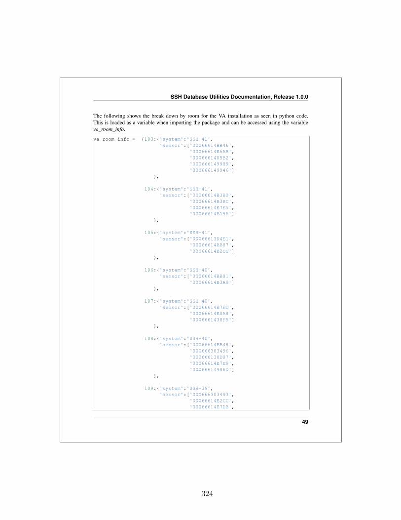
SSH Database Utilities Documentation, Release 1.0.0
The following shows the break down by room for the VA installation as seen in python code.This is loaded as a variable when importing the package and can be accessed using the variableva_room_info.
va_room_info = {103:{'system':'SSH-41','sensor':['00066614BB46',
'00066614E6AB','0006661405B2','000666149989','000666149946']
},
104:{'system':'SSH-41','sensor':['00066614B3B0',
'00066614B3BC','00066614E7E5','00066614B15A']
},
105:{'system':'SSH-41','sensor':['00066613D4E1',
'00066614BB87','00066614E2CC']
},
106:{'system':'SSH-40','sensor':['00066614BB81',
'00066614B3A9']},
107:{'system':'SSH-40','sensor':['00066614E7EC',
'00066614E0A8','0006661438F5']
},
108:{'system':'SSH-40','sensor':['00066614BB48',
'000666303496','000666138D07','00066614E7E9','00066614986D']
},
109:{'system':'SSH-39','sensor':['000666303493',
'00066614E2CC','00066614E7DB',
49
324

SSH Database Utilities Documentation, Release 1.0.0
'000666143087','0006661497E3']
},
110:{'system':'SSH-39','sensor':['00066614BB7C',
'00066614E272','00066614B3A5','00066614394B','00066614996F','0006661497E8']
},
111:{'system':'SSH-39','sensor':['000666138F1E',
'000666138D2C','000666143081']
},
112:{'system':'SSH-39','sensor':['00066614B3B3',
'00066614BB45','00066614999F']
},
113:{'system':'SSH-38','sensor':['0006661400E5',
'00066614BB89','000666142F31','000666303486','00066614B3B5']
},
114:{'system':'SSH-38','sensor':['00066614C7AE',
'000666138D9C']},
115:{'system':'SSH-38','sensor':['00066614DC67',
'000666142E73']},
116:{'system':'SSH-37','sensor':['00066614BB90',
'00066613C925','0006661499A6']
50
325

SSH Database Utilities Documentation, Release 1.0.0
},
117:{'system':'SSH-37','sensor':['00066613D665',
'000666303495','0006661499B5','000666142F24']
},
118:{'system':'SSH-37','sensor':['00066614E6D0',
'00066614D0A3','000666139700','00066614B3B1','000666149983']
},
119:{'system':'SSH-37','sensor':['000666143B49',
'00066614B94A','0006661499B5','00066614B3A1','0006661499B6','0006661497A5']
},
120:{'system':'SSH-36','sensor':['000666303492',
'00066614E241','00066614998E']
},
120:{'system':'SSH-36','sensor':['000666303492',
'00066614E241','00066614998E']
},
121:{'system':'SSH-36','sensor':['00066614BB8F',
'00066614BB7E','000666303485','0006661499AF']
},
122:{'system':'SSH-36','sensor':['00066614E687',
51
326

SSH Database Utilities Documentation, Release 1.0.0
'00066614B3A1','00066614E687','000666149981']
},}
52
327

PYTHON MODULE INDEX
aactivity_density, 1
ddata_dumper, 4dispersion_ratio, 7
eevent, 9event_processor, 12events_by_day, 21
mmax_amplitude, 24metrics, 28monitored_days, 31
nnan_density, 34
rrate_of_dispersion, 40record_categorize, 36
ssignal_energy, 38std_wave, 42
vva_room_info, 47value_jump, 45
53
328

Appendix N
FEEL Python Package Documentation
This presents the documentation for the Python package that implements the
FEEL Algorithm presented in Chapter 5.
329

FEEL DocumentationRelease 1.0.0
Benjamin T. Davis
May 04, 2016
330

CONTENTS
1 License 1
2 Low-Pass FIR Filter 2
3 Resample 7
4 Transfer Function Estimate 9
5 Force 11
6 Location 14
7 How To...? 187.1 FIR Filter a Signal . . . . . . . . . . . . . . . . . . . . . . . . . . . . . . . . . . 187.2 Plot a FIR Filter . . . . . . . . . . . . . . . . . . . . . . . . . . . . . . . . . . . 197.3 Resample a Signal . . . . . . . . . . . . . . . . . . . . . . . . . . . . . . . . . . 217.4 Make a Transfer Function . . . . . . . . . . . . . . . . . . . . . . . . . . . . . . 227.5 Plot a Transfer Function . . . . . . . . . . . . . . . . . . . . . . . . . . . . . . . 227.6 Calculate Force . . . . . . . . . . . . . . . . . . . . . . . . . . . . . . . . . . . . 237.7 Find Impact Location . . . . . . . . . . . . . . . . . . . . . . . . . . . . . . . . 25
8 Code Example 28
Python Module Index 38
i
331

CHAPTER
ONE
LICENSE
Copyright (c) 2016 Benjamin T. Davis. All rights reserved.
Redistribution and use in source and binary forms, with or without modification, are permittedprovided that the following conditions are met:
1. Redistributions of source code must retain the above copyright notice, this list of conditions andthe following disclaimer.
2. Redistributions in binary form must reproduce the above copyright notice, this list of condi-tions and the following disclaimer in the documentation and/or other materials provided with thedistribution.
3. Neither the name of the copyright holder nor the names of its contributors may be used toendorse or promote products derived from this software without specific prior written permission.
THIS SOFTWARE IS PROVIDED BY THE COPYRIGHT HOLDERS AND CONTRIBUTORS“AS IS” AND ANY EXPRESS OR IMPLIED WARRANTIES, INCLUDING, BUT NOT LIM-ITED TO, THE IMPLIED WARRANTIES OF MERCHANTABILITY AND FITNESS FOR APARTICULAR PURPOSE ARE DISCLAIMED. IN NO EVENT SHALL THE COPYRIGHTHOLDER OR CONTRIBUTORS BE LIABLE FOR ANY DIRECT, INDIRECT, INCIDENTAL,SPECIAL, EXEMPLARY, OR CONSEQUENTIAL DAMAGES (INCLUDING, BUT NOT LIM-ITED TO, PROCUREMENT OF SUBSTITUTE GOODS OR SERVICES; LOSS OF USE, DATA,OR PROFITS; OR BUSINESS INTERRUPTION) HOWEVER CAUSED AND ON ANY THE-ORY OF LIABILITY, WHETHER IN CONTRACT, STRICT LIABILITY, OR TORT (INCLUD-ING NEGLIGENCE OR OTHERWISE) ARISING IN ANY WAY OUT OF THE USE OF THISSOFTWARE, EVEN IF ADVISED OF THE POSSIBILITY OF SUCH DAMAGE.
1
332

CHAPTER
TWO
LOW-PASS FIR FILTER
Author: Benjamin T. Davis, NSF Graduate Research Fellow <[email protected]>
Date: 2015 May 1
2
333

FEEL Documentation, Release 1.0.0
lowpassfir.applyfilter(data, taps, a)Applies a low-pass finite impulse response filter to clean digital acceleration and force data
Parameters
• data (array-like) – The detrended data captured from a system (e.g.force) where column is the sensor and row is time step
• taps (1D array-like) – The values of the taps of the low pass FIR filter;can get the taps using design()
• a (float) – The denominator coefficient for the filter; can get the tapsusing design()
Returns
• fdata (array) – The filtered data
• delay (float) – The phase delay in points from the beginning of the sig-nal; to get the delay in seconds, divide value by sampling frequency; thefiltering process corrupts part of the record, so shift the record by thisvalue like this fdata[delay:]
Notes
•The way the record shift is calculated here differs from that of the reference mate-rial. This is due to some experimenting with the shifting value that determined forceestimations are more accurate with the version presented here.
References
http://wiki.scipy.org/Cookbook/FIRFilter
3
334

FEEL Documentation, Release 1.0.0
lowpassfir.design(fs, trans_hz=10, ripple_db=160, cutoff_hz=208, rv=’filter’)Designs a low-pass finite impulse response filter for cleaning digital acceleration and forcedata
Parameters
• fs (float) – Sampling frequency for the data in Hz
• trans_hz (int or float | optional | default = 10) – Transition width frompass to stop of the filter in Hz
• ripple_db (int or float | optional | default = 160) – Desired attenuationof the stop band in dB
• cutoff_hz (int or float | optional | default = 208) – Cut off frequency forthe filter in Hz; it is recommended that this value is slightly higher thanthe desired Nyquist Rate, e.g. (0.5*fs)+8
• rv (str | optional | default = ‘filter’) – Specified return values the userwants filter -> taps, a params -> taps, a, width, beta
Returns
• taps (1D array-like) – The values of the taps of the low pass FIR filter
• a (float) – The denominator coefficient for the filter
• width (float) – Transition width relative to Nyquist Rate
• beta (float) – Kaiser window beta parameter used
References
http://wiki.scipy.org/Cookbook/FIRFilter
4
335

FEEL Documentation, Release 1.0.0
lowpassfir.plotfiltercoeff(taps)Plots the FIR filter coefficients
Parameters taps (1D array-like) – The values of the taps of the low pass FIRfilter; can get the taps using design()
Returns axis (<matplotlib.axes.AxesSubplot>) – The axis handle for the currentplot; can be used to adjust the plot visuals
Notes
•The axis default to light gray in color
•Change various features of the plot using axis; e.g.
>>> pyplot.setp(axis.lines, color='r', linewidth=2.0, linestyle='-')
References
http://wiki.scipy.org/Cookbook/FIRFilter
http://matplotlib.org/users/pyplot_tutorial.html
5
336

FEEL Documentation, Release 1.0.0
lowpassfir.plotfreqresponse(taps, fs)Plots the FIR filter frequency response
Parameters
• taps (1D array-like) – The values of the taps of the low pass FIR filter;can get the taps using design()
• fs (int or float) – Sampling frequency for the data; same as used indesign()
Returns axis (<matplotlib.axes.AxesSubplot>) – The axis handle for the currentplot; can be used to adjust the plot visuals
Notes
•The axis default to light gray in color
•Change various features of the plot using axis; e.g.
>>> pyplot.setp(axis.lines, color='r', linewidth=2.0, linestyle='-')
References
http://wiki.scipy.org/Cookbook/FIRFilter
http://matplotlib.org/users/pyplot_tutorial.html
6
337

CHAPTER
THREE
RESAMPLE
Author: Benjamin T. Davis, NSF Graduate Research Fellow <[email protected]>
Date: 2015 May 1
7
338

FEEL Documentation, Release 1.0.0
resample.resample(data, oldfs, newfs, trans_hz=10, ripple_db=160, cutoff_hz=208)Resamples data from and old rate to a new rate using the Fourier Method, after applying aFIR filter to clean the data
Warning: Function has only been tested to work for downsampling!
Parameters
• data (array-like) – The detrended data captured from a system (e.g.force) where column is the sensor and row is time step
• oldfs (float) – Original sampling frequency for the data in Hz
• newfs (float) – New sampling frequency for the data in Hz
• trans_hz (int or float | optional | default = 10) – Transition width frompass to stop of the filter in Hz
• ripple_db (int or float | optional | default = 160) – Desired attenuationof the stop band in dB
• cutoff_hz (int or float | optional | default = 208) – Cut off frequency forthe filter in Hz; it is recommended that this value is slightly higher thanthe desired Nyquist Rate, e.g. (0.5*fs)+8
Returns rdata (1D array) – The resampled data that has been adjusted for phasedelay
Notes
•function has only been tested and verified to work when downsampling
•if you are interested in seeing more specifics about the filter, refer to lowpassfir func-tions
References
http://docs.scipy.org/doc/scipy-0.15.1/reference/generated/scipy.signal.resample.html
8
339

CHAPTER
FOUR
TRANSFER FUNCTION ESTIMATE
Author: Benjamin T. Davis, NSF Graduate Research Fellow <[email protected]>
Date: 2015 April 30
9
340

FEEL Documentation, Release 1.0.0
tfestimate.tfestimate(x, y, fs, nfft=2048, noverlap=1024)Estimates the transfer function using the average of two different methods to calculate thetransfer function
Parameters
• x (1D array-like) – The input for the system (e.g. force)
• y (1D array-like) – The output of the system (e.g. accelerations) corre-sponding to the input x
• fs (int or float) – Sampling frequency for both the input and output
• nfft (int | optional | default = 2048) – Number of data points used ineach block for FFT
• noverlap (int | optional | default = 1024) – Number of overlapping datapoints used for Welch’s Average Periodogram Method
Returns
• freq (1D array) – The frequencies corresponding to each point of thetransfer function estimate
• tfe (1D array) – The values of the transfer function estimate
Notes
•x and y should be captured at the same sampling frequency
•utilizes Welch‘s Average Periodogram Method
•typically one would want to display the transfer function in decibel units; to convert todB perform 20*log10(tfe)
References
http://matplotlib.org/api/mlab_api.html?highlight=psd#matplotlib.mlab.psd
http://matplotlib.org/api/mlab_api.html?highlight=psd#matplotlib.mlab.csd
Bendat, J. S., and Piersol, A. G. (2000). Random Data: Analysis and Measurement Proce-dures. Wiley. New York.
Ewins, D.J. (2000). Modal Testing: Theory, Practice, and Application. Research StudiesPress Ltd. p.238-239.
10
341

CHAPTER
FIVE
FORCE
Author: Benjamin T. Davis, NSF Graduate Research Fellow <[email protected]>
Date: 2015 April 30
11
342

FEEL Documentation, Release 1.0.0
force.estimate(accel, tfe, nfft=2048, rmtrend=False)Estimates the force of impact from acceleration data
Parameters
• accel (1D array-like) – The detrended accelerations captured from a sys-tem
• tfe (1D array-like) – The values of the transfer function estimate relatingforce and acceleration; these are found using feel.tfestimate()
• nfft (int | optional | default = 2048) – Number of data points used in theFFT
• rmtrend (boolean | optional | default = False) – Whether or not to re-move trend (detrend) of the force estimate before returning the data; usesscipy.signal.detrend() with default settings
Returns f_hat (array) – The detrended impact force estimate
Notes
•Only uses the first n points of the acceleration signal, where n is the number of pointsof the tfe
References
http://docs.scipy.org/doc/numpy/reference/routines.fft.html
http://docs.scipy.org/doc/scipy-0.15.1/reference/generated/scipy.signal.detrend.html
12
343

FEEL Documentation, Release 1.0.0
force.magnitude(f_hat)Determines the magnitude of the force estimate. Grabs the two best matching force estimatepairs (based on correlations) and uses the real part of the complex conjugate to calculate themagnitude.
Parameters f_hat (array) – The force estimates for a location with rows beingthe sensor and columns being the data points
Returns f (float) – The force estimate magnitude
Notes
•it is easiest to take the outputs from force_estimate and usenumpy.vstack((force1, force2)) to create the f_hats array
13
344

CHAPTER
SIX
LOCATION
Author: Benjamin T. Davis, NSF Graduate Research Fellow <[email protected]>
Date: 2015 June 10
14
345

FEEL Documentation, Release 1.0.0
location.forcedev(f_hats)Calculates the deviation of force estimates for each provided location using real portion ofthe estimate only
Parameters f_hats (dict) – The detrended impact force estimates for each sensorat each location of form
>>> f_hats = {1: [force11 force12], 2:[force21 force22]}
where the dict key is the location designation, and the dict value is an arraywhere rows indicate sensor and column indicate points in the force estimates
Returns
L (dict) – The values for each location in f_hats of form
>>> L = {1: dev1, 2: dev2}
where lowest deviation value is the location of impact
Notes
•It is easiest to take the outputs from force_estimate and use numpy.vstack((force11,force12)) to create each dictionary value
•It is also best to use this method by first taking a window around the peak of the forceestimate for each sensor record in f_hats
15
346

FEEL Documentation, Release 1.0.0
location.forcecorr(f_hats)Calculates the correlation of force estimates for each provided location by calculating thecorrelation coefficents of pairs of signals and grabbing the largest coefficient as the correla-tion for the location
Parameters f_hats (dict) – The detrended impact force estimates for each sensorat each location of form
>>> f_hats = {1: [force11 force12], 2:[force21 force22]}
where the dict key is the location designation, and the dict value is an arraywhere rows indicate sensor and column indicate points in the force estimates
Returns
L (dict) – The values for each location in f_hats of form
>>> L = {1: corr1, 2: corr2}
where highest correlation value is the location of impact
Notes
•It is easiest to take the outputs from force_estimate and usenumpy.vstack((force11, force12)) to create each dictionary value
16
347

FEEL Documentation, Release 1.0.0
location.locate(L, ctype=’corr’)Determines the location of impact
Parameters
• L (dict) – The values for each location in f_hats of form {1: dev1, 2:dev2}
• ctype (str) – The force comparision type used
std -> if results are from forcedev
corr -> if results are from forcecorr
Returns L_hat (any type) – The location of impact; type is dependent on the keytype given in the dictionary L
17
348

CHAPTER
SEVEN
HOW TO...?
Here are various topics to help you on your way to using the feel package to its fullest.
7.1 FIR Filter a Signal
Sometimes a signal contains a lot of high-frequency noise that is unnecessary for the FEEL Al-gorithm and it just creates noisy transfer functions which in turn skew results. The feel packageprovides a simple way to clean these signals using lowpassfir().
Let’s say you have acceleration data, named signal, collected at a rate of 2000 Hz, sees a lot ofnoise once it passes the 500 Hz frequency. We would filter it like in the following.
from feel.lowpassfir import design, applyfilter
# design the filtertaps, a = design(fs=2000,
trans_hz=10,ripple_db=160,cutoff_hz=1008,rv='filter')
# apply the filterfdata, delay = applyfilter(data=signal,
taps=taps,a=a)
FIR Filters have a linear phase delay which allows one to easily remove the phase from the filteredsignal. This is done like in the following.
s = fdata[delay:]
A good tip is to make the cut-off frequency slightly higher than the Nyquist Frequency, or in otherwords slightly higher than half of the fs.
18
349

FEEL Documentation, Release 1.0.0
7.2 Plot a FIR Filter
When reporting about the filter one used, it is sometimes beneficial to provide plots showing thethe filter coefficients and frequency response. The feel package provides a simple way to cleanthese signals using lowpassfir().
7.2.1 Filter Coefficents
To plot the filter coefficients, do the following.
from feel.lowpassfir import design, plotfiltercoeff
# design the filtertaps, a = design(fs=2000,
trans_hz=10,ripple_db=160,cutoff_hz=208,rv='filter')
# now for plottingaxis = plotfiltercoeff(taps)
Figure 7.1 shows an example of what the filter coefficients look like when plotted.
7.2. Plot a FIR Filter 19
350
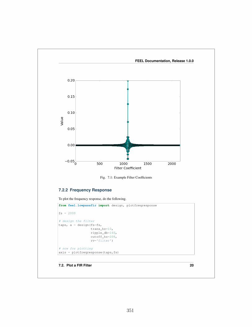
FEEL Documentation, Release 1.0.0
Fig. 7.1: Example Filter Coefficients
7.2.2 Frequency Response
To plot the frequency response, do the following.
from feel.lowpassfir import design, plotfreqresponse
fs = 2000
# design the filtertaps, a = design(fs=fs,
trans_hz=10,ripple_db=160,cutoff_hz=208,rv='filter')
# now for plottingaxis = plotfreqresponse(taps,fs)
7.2. Plot a FIR Filter 20
351
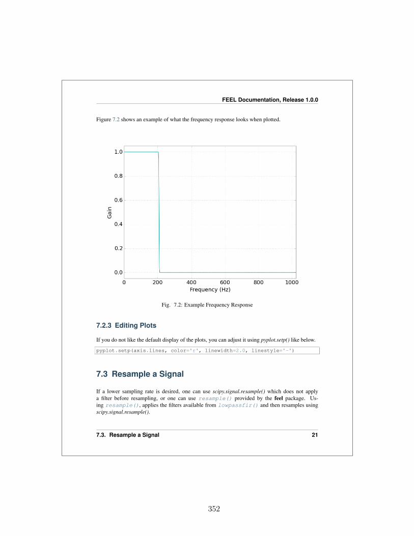
FEEL Documentation, Release 1.0.0
Figure 7.2 shows an example of what the frequency response looks when plotted.
Fig. 7.2: Example Frequency Response
7.2.3 Editing Plots
If you do not like the default display of the plots, you can adjust it using pyplot.setp() like below.
pyplot.setp(axis.lines, color='r', linewidth=2.0, linestyle='-')
7.3 Resample a Signal
If a lower sampling rate is desired, one can use scipy.signal.resample() which does not applya filter before resampling, or one can use resample() provided by the feel package. Us-ing resample(), applies the filters available from lowpassfir() and then resamples usingscipy.signal.resample().
7.3. Resample a Signal 21
352
FEEL Documentation, Release 1.0.0
For example, consider the following code where we want to resample the data from 2000 Hz to400 Hz.
from feel import resample
rdata = resample(data,oldfs=2000,newfs=400,trans_hz=10,ripple_db=160,cutoff_hz=208)
A good tip is to make the cut-off frequency slightly higher than the Nyquist Frequency, or in otherwords slightly higher than half of the newfs.
7.4 Make a Transfer Function
The basis of the FEEL Algorithm is based in manipulation of transfer functions. So naturally afunction, called tfestimate(), to easily generate said function is provided in the package. Seethe code snippet below where the variable input would the exciter of the system, and the variableoutput would be the measured response of the system.
from feel import tfestimate
freq, tfe = tfestimate(x=input,y=output,fs=500,nfft=2048,noverlap=1024)
Typically you would want to have an noverlap of half of the nfft which helps smooth out the transferfunction.
7.5 Plot a Transfer Function
Transfer functions are often displayed using decibels for the power value and Hertz for the fre-quency values. The code above gives freq in Hertz, but not tfe in decibels. For example, here ishow you would simply plot the output from tfestimate().
import numpy as npfrom matplotlib import pyplot as plt
tfe_db = 20 * np.log10(tfe)
7.4. Make a Transfer Function 22
353
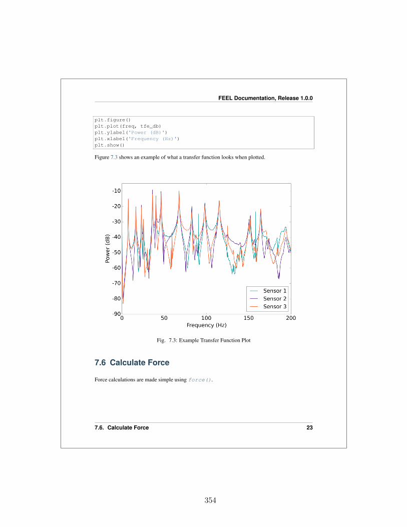
FEEL Documentation, Release 1.0.0
plt.figure()plt.plot(freq, tfe_db)plt.ylabel('Power (dB)')plt.xlabel('Frequency (Hz)')plt.show()
Figure 7.3 shows an example of what a transfer function looks when plotted.
Fig. 7.3: Example Transfer Function Plot
7.6 Calculate Force
Force calculations are made simple using force().
7.6. Calculate Force 23
354
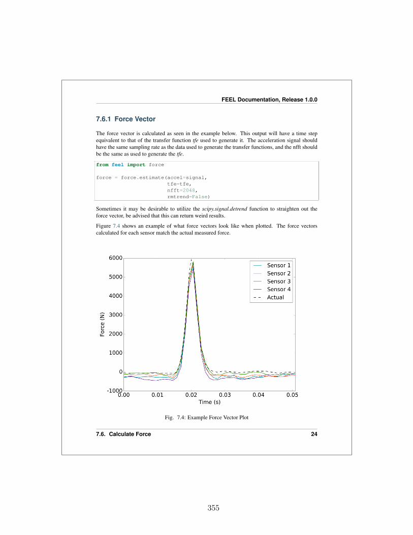
FEEL Documentation, Release 1.0.0
7.6.1 Force Vector
The force vector is calculated as seen in the example below. This output will have a time stepequivalent to that of the transfer function tfe used to generate it. The acceleration signal shouldhave the same sampling rate as the data used to generate the transfer functions, and the nfft shouldbe the same as used to generate the tfe.
from feel import force
force = force.estimate(accel=signal,tfe=tfe,nfft=2048,rmtrend=False)
Sometimes it may be desirable to utilize the scipy.signal.detrend function to straighten out theforce vector, be advised that this can return weird results.
Figure 7.4 shows an example of what force vectors look like when plotted. The force vectorscalculated for each sensor match the actual measured force.
Fig. 7.4: Example Force Vector Plot
7.6. Calculate Force 24
355
FEEL Documentation, Release 1.0.0
7.6.2 Force Magnitude
Each force vector has a peak magnitude which is considered to be the force of impact. This iscalculated by taking the minimum value of the local peak area and subtracting it from the maximumvalue of the local peak area. Luckily, feel provides a function to do just that. See the examplebelow.
from feel import force
magnitude = force.magnitude(force)
7.7 Find Impact Location
The location of impact can be determined using the force vectors from each sensor which ex-perience the event. This method requires a minimum of two sensor’s force vectors to work.Two techniques are shipped with the package. The author recommends the Force CorrelationMethod provided by location.forcecorr() as it is more robust, and will be the examplepresented. Alternatively, a second choice is to use the Force Deviation Method available fromlocation.forcedev().
7.7.1 Force Correlation Method
The author’s recommended method is demonstrated in the example below. Let’s start by gettingthe force vectors (see force.estimate()) of two sensors who are s1 and s2 respectively, forall two locations l1 and l2 using the transfer functions estimates (see tfestimate()) for eachof the locations to each of the sensors.
import numpy as npfrom feel import force, location
# location 1force_s1_l1 = force.estimate(accel=s1,
tfe=tfe_s1_l1,nfft=2048,rmtrend=False)
force_s2_l1 = force.estimate(accel=s2,tfe=tfe_s2_l1,nfft=2048,rmtrend=False)
# location 2force_s1_l2 = force.estimate(accel=s1,
7.7. Find Impact Location 25
356
FEEL Documentation, Release 1.0.0
tfe=tfe_s1_l2,nfft=2048,rmtrend=False)
force_s2_l2 = force.estimate(accel=s2,tfe=tfe_s2_l2,nfft=2048,rmtrend=False)
Then we make the f_hats dictionary where keys are location names and the values are the forcevectors of each sensor for that location.
f_hats = {l1: np.vstack((force_s1_l1, force_s1_l1))l2: np.vstack((force_s1_l2, force_s1_l2))}
Once that is done, invoke the function for the Force Correlation Method (seelocation.forcecorr()) to get correlation values for each location.
L = location.forcecorr(f_hats)
This will give a dictionary back where key is the location label and value is the correlation for thatlocation. Now apply the location.locate() function which will tell you which location theimpact occurred.
L_hat = location.locate(L,ctype='corr')
7.7.2 Plotting the Force Correlation Method
To visualize the location correlations, the author suggests using a bar plot where the x axis is thelocation labels (i.e. the keys of the L dictionary), and the y axis is the correlation value (i.e. thevalues of the L dictionary). Highlighting the location where the algorithm thinks the event occurredhelps make the location’s bar pop. Something like in Figure 7.5.
7.7. Find Impact Location 26
357
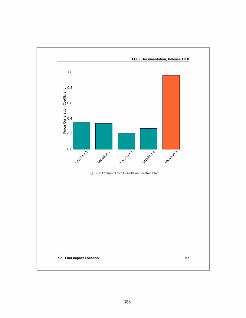
FEEL Documentation, Release 1.0.0
Fig. 7.5: Example Force Correlation Location Plot
7.7. Find Impact Location 27
358

CHAPTER
EIGHT
CODE EXAMPLE
A working example is provided along with the feel package that demonstrates its use. Look in thedirectory /feel/example/ for the Python code and the data files.
filename: example.py
"""Example using the FEEL Algorithm toolsuite
Author: Benjamin T. Davis, NSF Graduate Research FellowDate Created: 2015 May 1"""
import sysimport ossys.path.insert(0, os.path.abspath('../../')) # path to feel package
# relative to example.py
import numpy as npimport scipy.signal as signalfrom matplotlib import pyplot as plt
from feel import resample, tfestimate, force, location
#%% set constantsdt = 0.000488 # time step between samples
#%% Load data'''Location 1 Data'''# Accelerationfilename = './loc1/Acceleration.txt'loc1_accel = np.loadtxt(fname=filename, dtype=float, skiprows=7)
28
359
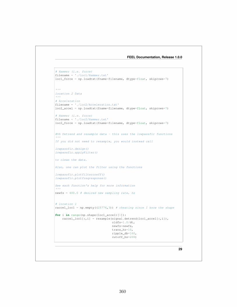
FEEL Documentation, Release 1.0.0
# Hammer (i.e. force)filename = './loc1/Hammer.txt'loc1_force = np.loadtxt(fname=filename, dtype=float, skiprows=7)
'''location 2 Data'''# Accelerationfilename = './loc2/Acceleration.txt'loc2_accel = np.loadtxt(fname=filename, dtype=float, skiprows=7)
# Hammer (i.e. force)filename = './loc2/Hammer.txt'loc2_force = np.loadtxt(fname=filename, dtype=float, skiprows=7)
#%% Detrend and resample data - this uses the lowpassfir functions'''If you did not need to resample, you would instead call
lowpassfir.design()lowpassfir.applyFilter()
to clean the data.
Also, one can plot the filter using the functions
lowpassfir.plotfiltercoeff()lowpassfir.plotfreqresponse()
See each function's help for more information'''newfs = 400.0 # desired new sampling rate, hz
# location 1raccel_loc1 = np.empty((25776,3)) # cheating since I know the shape
for i in range(np.shape(loc1_accel)[1]):raccel_loc1[:,i] = resample(signal.detrend(loc1_accel[:,i]),
oldfs=1.0/dt,newfs=newfs,trans_hz=10,ripple_db=160,cutoff_hz=208)
29
360

FEEL Documentation, Release 1.0.0
rforce_loc1 = resample(signal.detrend(loc1_force),oldfs=1.0/dt,newfs=newfs,trans_hz=10,ripple_db=160,cutoff_hz=208)
rforce_loc1 *= 10.350 # convert from volts to lb of force hammer
# plot location 1 dataplt.figure()plt.subplot(4,1,1)plt.plot(raccel_loc1[:,0])plt.ylim((-0.6,0.6))plt.xlim((0,len(raccel_loc1[:,0])))plt.title('Location 1 - ai0')plt.ylabel('Accel (g)')plt.subplot(4,1,2)plt.plot(raccel_loc1[:,1])plt.ylim((-0.6,0.6))plt.xlim((0,len(raccel_loc1[:,1])))plt.title('Location 1 - ai1')plt.ylabel('Accel (g)')plt.subplot(4,1,3)plt.plot(raccel_loc1[:,2])plt.ylim((-0.6,0.6))plt.xlim((0,len(raccel_loc1[:,2])))plt.title('Location 1 - ai2')plt.ylabel('Accel (g)')plt.subplot(4,1,4)plt.xlim((0,len(rforce_loc1)))plt.plot(rforce_loc1)plt.title('Location 1 - Force')plt.ylabel('Force (lb)')plt.xlabel('Points')plt.tight_layout()plt.show()
# location 2raccel_loc2 = np.empty((25776,3)) # cheating since I know the shape
for i in range(np.shape(loc2_accel)[1]):raccel_loc2[:,i] = resample(signal.detrend(loc2_accel[:,i]),
oldfs=1.0/dt,newfs=newfs,
30
361

FEEL Documentation, Release 1.0.0
trans_hz=10,ripple_db=160,cutoff_hz=208)
rforce_loc2 = resample(signal.detrend(loc2_force),oldfs=1.0/dt,newfs=newfs,trans_hz=10,ripple_db=160,cutoff_hz=208)
rforce_loc2 *= 10.350 # convert from volts to lb of force hammer
# plot location 2 dataplt.figure()plt.subplot(4,1,1)plt.plot(raccel_loc2[:,0])plt.ylim((-0.6,0.6))plt.xlim((0,len(raccel_loc2[:,0])))plt.title('Location 2 - ai0')plt.ylabel('Accel (g)')plt.subplot(4,1,2)plt.plot(raccel_loc2[:,1])plt.ylim((-0.6,0.6))plt.xlim((0,len(raccel_loc2[:,1])))plt.title('Location 2 - ai1')plt.ylabel('Accel (g)')plt.subplot(4,1,3)plt.plot(raccel_loc2[:,2])plt.ylim((-0.6,0.6))plt.xlim((0,len(raccel_loc2[:,2])))plt.title('Location 2 - ai2')plt.ylabel('Accel (g)')plt.subplot(4,1,4)plt.xlim((0,len(rforce_loc2)))plt.plot(rforce_loc2)plt.title('Location 2 - Force')plt.ylabel('Force (lb)')plt.xlabel('Points')plt.tight_layout()plt.show()
#%% Estimate transfer functionsnfft = 2048 # size of FFT window, typically best as a power of 2noverlap = nfft / 2 # overlap of Welch method, typically half of nfft
31
362

FEEL Documentation, Release 1.0.0
# Location 1freq_ai0, loc1_ai0_tf = tfestimate(x=rforce_loc1,
y=raccel_loc1[:,0],fs=newfs,nfft=nfft,noverlap=noverlap)
freq_ai1, loc1_ai1_tf = tfestimate(x=rforce_loc1,y=raccel_loc1[:,1],fs=newfs,nfft=nfft,noverlap=noverlap)
freq_ai2, loc1_ai2_tf = tfestimate(x=rforce_loc1,y=raccel_loc1[:,2],fs=newfs,nfft=nfft,noverlap=noverlap)
# plot location 1 TFplt.figure()plt.plot(freq_ai0, 20*np.log10(loc1_ai0_tf), label='ai0')plt.plot(freq_ai1, 20*np.log10(loc1_ai1_tf), label='ai1')plt.plot(freq_ai2, 20*np.log10(loc1_ai2_tf), label='ai2')plt.legend()plt.title('Location 1 Transfer Functions')plt.xlabel('Frequency (Hz)')plt.ylabel('Power (dB)')plt.show()
# Location 2freq_ai0, loc2_ai0_tf = tfestimate(x=rforce_loc2,
y=raccel_loc2[:,0],fs=newfs,nfft=nfft,noverlap=noverlap)
freq_ai1, loc2_ai1_tf = tfestimate(x=rforce_loc2,y=raccel_loc2[:,1],fs=newfs,nfft=nfft,noverlap=noverlap)
freq_ai2, loc2_ai2_tf = tfestimate(x=rforce_loc2,y=raccel_loc2[:,2],
32
363
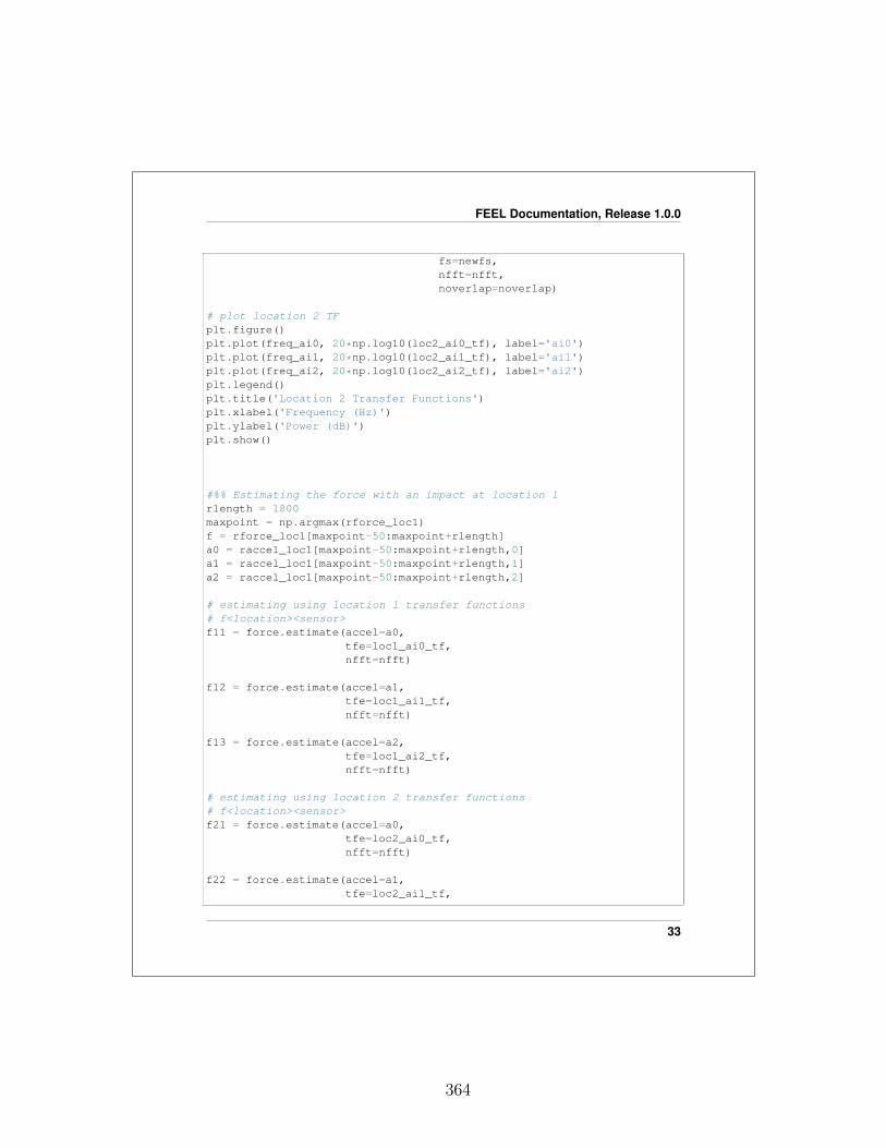
FEEL Documentation, Release 1.0.0
fs=newfs,nfft=nfft,noverlap=noverlap)
# plot location 2 TFplt.figure()plt.plot(freq_ai0, 20*np.log10(loc2_ai0_tf), label='ai0')plt.plot(freq_ai1, 20*np.log10(loc2_ai1_tf), label='ai1')plt.plot(freq_ai2, 20*np.log10(loc2_ai2_tf), label='ai2')plt.legend()plt.title('Location 2 Transfer Functions')plt.xlabel('Frequency (Hz)')plt.ylabel('Power (dB)')plt.show()
#%% Estimating the force with an impact at location 1rlength = 1800maxpoint = np.argmax(rforce_loc1)f = rforce_loc1[maxpoint-50:maxpoint+rlength]a0 = raccel_loc1[maxpoint-50:maxpoint+rlength,0]a1 = raccel_loc1[maxpoint-50:maxpoint+rlength,1]a2 = raccel_loc1[maxpoint-50:maxpoint+rlength,2]
# estimating using location 1 transfer functions# f<location><sensor>f11 = force.estimate(accel=a0,
tfe=loc1_ai0_tf,nfft=nfft)
f12 = force.estimate(accel=a1,tfe=loc1_ai1_tf,nfft=nfft)
f13 = force.estimate(accel=a2,tfe=loc1_ai2_tf,nfft=nfft)
# estimating using location 2 transfer functions# f<location><sensor>f21 = force.estimate(accel=a0,
tfe=loc2_ai0_tf,nfft=nfft)
f22 = force.estimate(accel=a1,tfe=loc2_ai1_tf,
33
364

FEEL Documentation, Release 1.0.0
nfft=nfft)
f23 = force.estimate(accel=a2,tfe=loc2_ai2_tf,nfft=nfft)
# form the dictionary for force_location# location #: array((sensor) x (npoints in force_estimate))# aka row is sensor, column is point in force estimate for each entryf_hats = {1:np.vstack((f11,f12,f13)), 2:np.vstack((f21,f22,f23))}
L = location.forcecorr(f_hats) # determines the force correlations
x = []y = []for key, val in L.items():
x.append(key)y.append(val)
time1 = np.array(range(0,len(f))) * dttime2 = np.array(range(0,len(f11))) * dt * 2.0
plt.figure()
# plot actual force of impactplt.subplot(4,1,1)plt.plot(time1, f, label='Actual')plt.title('Actual Impact at Location 1')plt.xlabel('Time (s)')plt.ylabel('Force (N)')
# plot location 1 force estimatesplt.subplot(4,1,2)plt.plot(time2, f11, label='ai0')plt.plot(time2, f12, label='ai1')plt.plot(time2, f13, label='ai2')plt.legend()plt.title('Location 1 Force Estimates (L1 TF)')plt.xlabel('Time (s)')plt.ylabel('Force (N)')
# plot location 2 force estimatesplt.subplot(4,1,3)plt.plot(time2, f21, label='ai0')plt.plot(time2, f22, label='ai1')plt.plot(time2, f23, label='ai2')plt.legend()
34
365

FEEL Documentation, Release 1.0.0
plt.title('Location 2 Force Estimates (L2 TF)')plt.xlabel('Time (s)')plt.ylabel('Force (N)')
# event localization# locate function gives the location numberplt.subplot(4,1,4)width = 0.8plt.bar(x,y, width=0.8, align='center')plt.title('Impact Occurred at Location %s' %location.locate(L))plt.xlabel('Location')plt.ylabel('Force Correlation')axis = plt.gca()axis.xaxis.set_ticks([1,2])axis.xaxis.set_ticklabels(['Loc %s'%x[0],'Loc %s'%x[1]])
plt.tight_layout()
plt.show()
#%% Estimating the force with an impact at location 2rlength = 1800maxpoint = np.argmax(rforce_loc2)f = rforce_loc2[maxpoint-50:maxpoint+rlength]a0 = raccel_loc2[maxpoint-50:maxpoint+rlength,0]a1 = raccel_loc2[maxpoint-50:maxpoint+rlength,1]a2 = raccel_loc2[maxpoint-50:maxpoint+rlength,2]
# estimating using location 1 transfer functions# f<location><sensor>f11 = force.estimate(accel=a0,
tfe=loc1_ai0_tf,nfft=nfft)
f12 = force.estimate(accel=a1,tfe=loc1_ai1_tf,nfft=nfft)
f13 = force.estimate(accel=a2,tfe=loc1_ai2_tf,nfft=nfft)
# estimating using location 2 transfer functions# f<location><sensor>f21 = force.estimate(accel=a0,
35
366
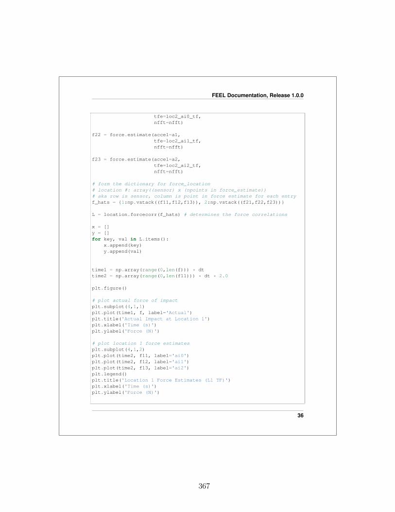
FEEL Documentation, Release 1.0.0
tfe=loc2_ai0_tf,nfft=nfft)
f22 = force.estimate(accel=a1,tfe=loc2_ai1_tf,nfft=nfft)
f23 = force.estimate(accel=a2,tfe=loc2_ai2_tf,nfft=nfft)
# form the dictionary for force_location# location #: array((sensor) x (npoints in force_estimate))# aka row is sensor, column is point in force estimate for each entryf_hats = {1:np.vstack((f11,f12,f13)), 2:np.vstack((f21,f22,f23))}
L = location.forcecorr(f_hats) # determines the force correlations
x = []y = []for key, val in L.items():
x.append(key)y.append(val)
time1 = np.array(range(0,len(f))) * dttime2 = np.array(range(0,len(f11))) * dt * 2.0
plt.figure()
# plot actual force of impactplt.subplot(4,1,1)plt.plot(time1, f, label='Actual')plt.title('Actual Impact at Location 1')plt.xlabel('Time (s)')plt.ylabel('Force (N)')
# plot location 1 force estimatesplt.subplot(4,1,2)plt.plot(time2, f11, label='ai0')plt.plot(time2, f12, label='ai1')plt.plot(time2, f13, label='ai2')plt.legend()plt.title('Location 1 Force Estimates (L1 TF)')plt.xlabel('Time (s)')plt.ylabel('Force (N)')
36
367

FEEL Documentation, Release 1.0.0
# plot location 2 force estimatesplt.subplot(4,1,3)plt.plot(time2, f21, label='ai0')plt.plot(time2, f22, label='ai1')plt.plot(time2, f23, label='ai2')plt.legend()plt.title('Location 2 Force Estimates (L2 TF)')plt.xlabel('Time (s)')plt.ylabel('Force (N)')
# event localization# locate function gives the location numberplt.subplot(4,1,4)width = 0.8plt.bar(x,y, width=0.8, align='center')plt.title('Impact Occurred at Location %s' %location.locate(L))plt.xlabel('Location')plt.ylabel('Force Correlation')axis = plt.gca()axis.xaxis.set_ticks([1,2])axis.xaxis.set_ticklabels(['Loc %s'%x[0],'Loc %s'%x[1]])
plt.tight_layout()
plt.show()
37
368

PYTHON MODULE INDEX
fforce, 10
llocation, 13lowpassfir, 1
rresample, 6
ttfestimate, 8
38
369