characterization of potential impact of speed limit enforcement on

Characterization of Potential Impact of Speed limit Enforcement on Emissions Reduction

Mohamadreza Farzaneh, Ph.D., P.E. * Center for Air Quality Studies, Texas Transportation Institute

1106 Clayton Lane, Suite 300E, Austin, TX 78723 Tel.: (512) 467-0946 Fax.: (512) 467-8971 Email: [email protected]

and

Josias Zietsman, Ph.D., P.E. Center for Air Quality Studies, Texas Transportation Institute

Tel.: (979) 458-3476 Fax.: (979) 845-7548 Email: [email protected]

Total words: 4377 + (6 figures and 4 tables) × 250 = 6,877

* Corresponding author

TRB 2012 Annual Meeting Paper revised from original submittal.

Farzaneh and Zietsman

2

ABSTRACT

The main objectives of this paper are twofold; first, the paper presents an approach to combine field data and microscopic emissions modeling to answer a transportation air quality policy issue. The study then uses this approach to evaluate the potential benefits of speed limit enforcement on vehicle emissions on high-speed roads.

The analytical approach used for this investigation involved performing two parallel phases - a field analysis phase based on field collected GPS data and a modeling analysis based on MOVES default drive schedules. Two highway speed limits were included in the analysis. The results show a modest increase of CO2 and fuel consumption for both speed limits. NOx and THC were increased more than 10% as the result of exceeding the speed limit. PM2.5 also showed a sizeable increase in the range of 10% to 36%. With an average increase of approximately 50%, CO showed the highest increase among all the pollutants.


3

INTRODUCTION

The U.S. Environmental Protection Agency (EPA) designates the areas that do not meet the National Ambient Air Quality Standards (NAAQS) as nonattainment areas. These areas must submit air quality plans, known as State Implementation Plans (SIPs), showing how they will attain the standards. If they fail to do this, they face sanctions and other penalties, such as the possible loss of highway funds, under the Clean Air Act Amendments of 1990 (CAAA). Many of these nonattainment areas have used, or attempted to use, various strategies in their SIPs to reduce emissions. These strategies include vehicle inspection and maintenance (I/M) programs, transportation control measures (TCM), clean fuel programs, etc.

The main purpose of this paper is to demonstrate the methodology of performing emission impact analysis for a specific policy question through a combination of fine GPS field data and second-by-second emissions modeling. The analytical approach used for this investigation involved performing two parallel phases - a field analysis phase based on field collected GPS data and a modeling analysis based on MOVES default drive schedules. Two highway speed limits were included in the analysis.

It is well known that a vehicle operating at higher speeds on a highway will generally emit higher amounts of pollutants as the engine will work at higher loads and consume more fuel; therefore, strategies targeted at lowering the average non-congested traffic flow speed would have large potential air quality benefits. The secondary purpose of this study is to investigate the potential benefits of speed limit enforcement on vehicle emissions on high-speed roads.

A field study and a modeling investigation were developed and executed to demonstrate examples of average changes in emissions of different pollutants as the results of exceeding posted speed limit. The field comprised of a limited real-world Global Positioning Satellite (GPS) data collection coupled with EPA’s new emissions estimation model, the MOtor Vehicle Emission Simulator (MOVES), to determine these changes. The modeling investigation was conducted based on the MOVES default drive schedules.

ENVIRONMENT AND SPEED REDUCTION

The majority of studies addressing the relationship between speed limit enforcement and emissions in the past five years have been performed in Europe. This section provides a review of observations and data collection performed on roads in The Netherlands, Portugal, and Switzerland.

In a study by Panis et al. (2006), the effectiveness of the various types of models available to researchers to conduct studies of speed limit effects on driver behavior was investigated. The researchers concluded that a traffic micro-simulation model is able to provide the necessary estimates of driving behavior, and that driver-specific speeds can be simulated in real time. This is considered a significant improvement compared with a single average speed for trips and road sections employed in macroscopic emission models. However, the input data required for such models are greater than for macroscopic models. In addition, validation of such detailed models is more complicated. Most of the validations to date have been conducted



4

against the measured traffic counts and speeds. Rarely have validations been made directly on modeled acceleration and deceleration. Efforts are required to further calibrate and validate methodologies before they can be reliably used as the basis for emissions estimation.

Panis et al. concluded that, overall, while speed management efforts effectively reduce the average speed of roadway traffic, its impact on vehicle emissions is complex. Frequent acceleration and deceleration movements in a network significantly reduce the effect of the reduced average speed on emissions. The net results are that active speed management has no significant impact on pollutant emissions.

The Portuguese study pertained to a traffic signalization project on a highway (Coelho et al. 2005). The case study site was on Highway N6 between the cities of Lisbon and Cascais, Portugal. The corridor is approximately 12.5 mi (20 km) long, with two approach lanes per direction. It is located along the coast and abuts several localities. The average annual daily traffic (AADT) is 37,000 and there are zones with different speed limits; 50, 60, and 70 k/h (30, 37, and 44 mph). At the two locations that were analyzed, the speed limit was set at 70 k/h.

There were 14 traffic control devices installed. The team collected signal and traffic parameters, such as length of the yellow, red, and green intervals, the approaching traffic volume and vehicle speed distribution. Field measurements of signal control and traffic stream variables were collected over several days using video cameras at two different locations for the site. Traffic volumes and speed in zones outside the influence of the signals were measured to verify whether drivers actually reduced their speed in the segments where traffic control devices are installed. The study showed that drivers did reduce their speed in the corridor.

This Portuguese observation confirms results from a Texas Transportation Institute (TTI 2002) study performed in Houston, TX, that showed average speeds would drop if speed limits are lowered or greater controls placed on a roadway. Speed limits were reduced on several Houston roadways. The TTI study indicated that although the average speeds had been reduced, the 55 mph level was not achieved. This proved consistent for all freeways that had been monitored. On a section of the I-610 North Loop that was previously signed at 60 mph, average speeds reduced from 60.2 mph to 57.8 mph during the non-peak daytime hours. During nighttime hours, the average speed decreased from 63.5 mph to 60.8 mph. However, the new averages were still above the posted speed limit by 2.8 mph and 5.8 mph respectively. An approximately seven-mile section of US 290 east of Beltway 8 previously signed at 65 mph resulted in an approximately 5-mph reduction in average speeds. However, the observed average speeds exceeded the 55-mph limit by 4 to 7 mph.

Coelho et al. concluded that speed limit strategies that prioritize enforcement of the speed limit tend to create more stops for all traffic, and therefore produce higher emissions. The control of speed violators increases with traffic flow. As a trade-off, overall traffic delay will also increase as well as the number of vehicles that are unfairly stopped, and, as a result, increases the generation of pollutant emissions. If the intent were to minimize the emissions consequences, then a more tolerant strategy for speed enforcement would need to be adopted.

This dilemma is highlighted by a New Zealand study. Povey et al. (2003) found that the perceived risk of being caught is a major determinant of drivers’ choice of speed. Speed limit reductions on a New Zealand roadway led to decreases in accidents, but this was achieved through an increase in speed infringement notices reflecting a decrease in enforcement tolerances and a policy of issuing tickets rather than warnings. The researchers also noted that high-impact



5

advertising and publicity campaigns to promote the harmful consequences of speeding supported enforcement activity.

In the Netherlands, dispersion models had suggested that traffic-related emissions on highways were substantially affected by the maximum driving speed. More strict speed limits on highways with many people living near the roadway would reduce exposure and related health effects. The objective of the Amsterdam study was to assess whether the policy to lower the maximum speed limit from 100 to 80 kph (62 to 50 mph) on a section of the Amsterdam ring highway had reduced measured traffic-related air pollution near the highway (Dijkema et al. 2008). Researchers collected traffic data from the national Department of Public Works along with roadside monitoring data from the Amsterdam Air Quality Monitoring Network. The network continuously monitors particulate matter (PM), oxides of nitrogen (NOx), and a proxy of soot at urban background and roadside locations in the Amsterdam city area. One of the roadside stations was located along the section of the ring highway under study and was where the speed limit intervention measurements were taken. The study concluded that PM emissions decreased after speeds were reduced on the section of the highway. No significant effect on NOx was observed.

In a Swiss study, Keller et al. (2008) investigated how emissions and ozone levels would have changed if the maximum speed limit on Swiss motorways were decreased from 120 to 80 kph (75 to 50 mph). The air quality model package MM5/CAMx was applied to two nested domains, both including Switzerland. Anthropogenic emissions were based on various European and Swiss data sources. The simulations for the reference case were based on current driving behavior. The research team concluded that the traffic speed reduction alone was not sufficient to significantly reduce ozone levels. However, it was noted that NOx and aerosol concentrations, traffic noise, and heavy accidents decrease in such a traffic scenario as well. These provide an additional benefit besides any small ozone reduction during summer smog conditions. The researchers also noted that more important for ozone reductions in Switzerland were the long-term emission developments in Switzerland, in the adjacent countries and, to some extent, in the entire northern hemisphere. This means that significantly greater reductions would occur from more broad, regional, or international efforts.

STUDY APPROACH

A field study and a modeling investigation were developed and executed to demonstrate examples of average changes in emissions of different pollutants as the results of exceeding posted speed limit. The field comprised of a limited real-world Global Positioning Satellite (GPS) data collection coupled with EPA’s new emissions estimation model, the MOtor Vehicle Emission Simulator (MOVES), to determine these changes. The modeling investigation was conducted based on the MOVES default drive schedules.

The analytical approach used for this section involved the execution of four tasks. Figure 1 shows the project flow diagram, and where the various tasks fit in the process. As shown in the flow diagram, this analysis is divided into two phases that were executed in parallel — a field analysis phase based on field collected GPS data and a modeling analysis based on MOVES



6

default drive schedules. The following section describes these tasks in detail. Both studies were performed based on the following common assumptions:

- only gasoline passenger cars and passenger trucks (SUVs, minivans, and pickup trucks)were used;

- all the vehicles use the same gasoline; - the emissions estimations are based on average ambient conditions for Travis County,

TX, in August; - the 2009 age distribution was used for both vehicle classes; and - a 50%-50% split was assumed for vehicle classes; based on vehicle sales estimates from

Annual Energy Outlook 2010 report (EIA 2010).

FIELD STUDY

EPA’s newest emissions model, MOVES, utilizes a disaggregate approach to estimate emissions rates and emissions inventories (EPA 2009). This disaggregate approach enables MOVES to perform estimations at different analysis levels. The model is currently available with only the national average driving patterns included in the default database of the model. Despite this, users can input customized drive schedules or equivalent operating mode distributions into the model for link-based analysis; i.e., project level analysis. This field study exploits this feature of the MOVES model by applying real-world speed profiles for scenarios representing speed limit compliant and noncompliant driving conditions.

For this purpose, the research team conducted a series of data collection efforts on a major highway in Austin, TX, metropolitan area. A mid-size passenger vehicle was equipped with a GPS unit and was driven multiple times on selected routes. The driver used the following driving instructions to generate the appropriate information for the required scenarios: speed limit compliant: do not exceed the speed limit while following the traffic flow in

the center or right lane; speed limit noncompliant: follow the traffic flow in the left lane; and drive safely and do not interrupt the traffic flow in any instance.

All the data collection runs occurred during the off-peak period between 10:00 a.m. and 1:00 p.m. Table 1 lists the study routes and the information for the different scenario runs. Figure 2 shows these routes on the area map. Both roadways (IH-35 and US 183) are major freeways that serve the Austin metro area. Speed limits on these roadways vary between 60 mph in urban areas to 65 mph in rural areas.

Each data collection run included driving in a loop while not exceeding the speed limit, i.e. compliant runs, followed immediately by a run following the traffic flow on the left most lane, i.e. noncompliant runs. Table 1 also includes the information for each run.

The GPS data file was imported into mapping software. Locations of the beginning and end points of the runs as well as the points of speed limit changes were marked on the map. The observations corresponding to each run were then extracted using these reference points. The



7

speed profiles of all runs were examined for errors and out-of-bound readings. This quality control showed no sign of error in the extracted speed profiles and therefore each speed profile was accepted as a drive schedule representing one of the scenarios shown in Table 1. The table also shows average speed and traveled distance of each run. Figure 3 presents a sample of these drive schedules.

The drive schedules were imported to the MOVES2010 model under the model’s project level analysis option. The age distribution of Texas light-duty gasoline vehicles were also imported to the model. The ambient conditions for an average day in August were obtained and used for all the MOVES runs. MOVES has two light-duty gasoline vehicle classes: passenger cars (source type 21), and passenger trucks (source type 31) including SUVs, minivans, and pick-up trucks. Both of these classes were included in the analysis. A 50%-50% split was used to aggregate the results to represent the majority of the light-duty gasoline vehicles.

The following pollutants were included in the analysis: NOx, carbon monoxide (CO), total hydrocarbons (THC), PM2.5, and carbon dioxide (CO2). NOx and THC are ozone precursors and thus have high importance in Texas while CO and PM2.5 are associated with health hazard to humans. CO2 is the main greenhouse gas contributing to the global climate change. CO2 is also directly related to fuel consumption and therefore its changes reflect changes in fuel consumption.

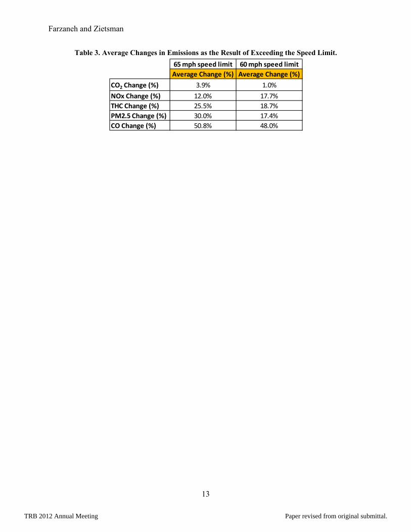
The results of the MOVES runs, grams of pollutants for each drive schedule normalized by the distance, grams per mile (g/mi) for a single representative vehicle, were calculated and organized by pollutant, scenario runs, and posted speed limits. The net difference and percentage changes in emissions for each scenario were calculated. Figure 4 and Figure 5 shows the distance-normalized emissions results of the average representative vehicle for each scenario. Table 2 presents the percent changes for each scenario run for the average representative vehicle. Table 3 lists the average percentage change for each speed limit (60 and 65 mph).

The results show a modest increase of CO2 for both speed limits. Fuel consumption is directly related to CO2 and therefore will have approximately the same percentage of increase. Both ozone precursors, NOx and THC, increased more than 10% as the result of exceeding the speed limit. PM2.5 also showed a sizeable increase in the range of 10% to 36%. With an average increase of approximately 50%, CO showed the highest increase among all the pollutants. The higher speed limit (65 mph) appears to have an increased impact on the CO2 changes, THC, and PM2.5; i.e., exceeding a 65 mph speed limit appears to result in a higher percentage change in emissions than exceeding a 60 mph speed limit.

In interpreting and using the results of this analysis, the limitation of the collected data and methodology should be considered. The relationship between traffic movement and emissions is a multidimensional issue. The main dimensions are – traffic demand (traffic volume), – average traffic speed, and – average driving behavior (i.e., the amount of acceleration and deceleration instances). Any change in one dimension is expected to influence the other dimensions as well, which might decrease or cancel out the intended benefits of the implemented measure. For example, lowering the average traffic speed via increased speed limit enforcement might increase the average distribution of acceleration maneuvers, which in turn will produce higher amount of emissions that exceed the reductions obtained from reducing average traffic speed.

The data collected and used in this investigation were obtained driving a single vehicle. While this approach provided real-world driving pattern data required for accurate estimation



8

analysis, however, it does not address the interaction of the vehicles. Specifically, it is assumed that, on average, all the vehicles will drive the same as the speed-limit-compliant driving behavior that was observed in this case study, if the posted speed limit is more effectively enforced. Other limitations that need to be taken into consideration are:

- The research team wanted to use field data as the basis of the study and did not have access to such data from vehicle classes other than light-duty vehicles; therefore the study only addressed emissions from light duty-vehicles.

- Since there is large variability in CO, CO2, NOx and PM2.5 emissions, uncertainty analysis of MOVES output is required to distinguish statistically significant effects of different speed limits. Sensitivity analysis of model assumptions would also help in identifying more robust effects. Such sensitivity analyses were beyond the scope of this study and were not included.

- Statistical tests of MOVES output under different scenarios need to be undertaken before making definitive assertions about the air quality effects of enforcing speed limits.

IMPACT OF SPEED FROM MOVES

In addition to the field study, the research team also examined the changes in emissions rates based on the default drive schedules that are incorporated in the current version of the MOVES model. These drive schedules represent national average drive schedules corresponding to different average speeds. The drive schedules are grouped by roadway type; i.e., rural or urban, and limited access (freeway and highway) or unlimited access (arterials). Since the focus of the study is the air quality impact of speed limit enforcement, the research team determined the urban limited access road type would best represent the desired conditions.

The required MOVES input files were prepared assuming the similar conditions that were used for the field study; i.e., average Texas age distribution for the light-duty gasoline vehicles, a 50%-50% split for cars and passenger trucks, etc. Similar to the field study, emissions of NOx, THC, CO, PM2.5, and CO2 were included in the analysis.

Using the above input information, the emissions rates for average speeds of 75, 70, 65, 60, and 55 mph were obtained for these pollutants. The percent changes in emissions rates as the result of exceeding the speed limit were calculated for 70, 65, 60, and 50 mph speed limits. For each speed limit, exceeding the speed limit by 5, 10, and 15 mph were included in the analysis where applicable. The highest speed bin in the MOVES model has an average speed of 75 mph, therefore this speed was the maximum speed included in this investigation. Table 4 shows the results of this analysis. Figure 6 shows the same results in graphical form.

As it was previously mentioned, the default drive schedules in the MOVES model for a vehicle class depends on the type of the facility and does not have any direct relationship with the speed limits. The results of this analysis should then be interpreted in light of this limitation. It is strongly recommended to take these results as an indication of the changes and not the final estimated changes. An approach similar to the field study in this project is a better method to produce accurate estimates of emissions changes. Overall, the modeling analysis results are in agreement with field observations; however, it appears that the benefits of enforcing lower speed limits (i.e. 55 and 50 mph) are not as considerable as speed limits higher than 60 mph.



9

CONCLUSIONS This paper demonstrates a unique application of GPS data collection and microscopic

emissions modeling to investigate the emission implication of a transportation policy issue. The paper shows how field GPS data collection can be combined with EPA’s MOVES model to answer a specific policy question. The demonstrated methodology is used to investigate the potential benefits of speed limit enforcement on vehicle emissions on high-speed roads.

A field study and a modeling investigation were developed and executed to demonstrate examples of average changes in emissions of different pollutants as the results of exceeding posted speed limit. The field comprised of a limited real-world Global Positioning Satellite (GPS) data collection coupled with EPA’s new emissions estimation model, the MOtor Vehicle Emission Simulator (MOVES), to determine these changes. The modeling investigation was conducted based on the MOVES default drive schedules. The results show a modest increase of CO2 and fuel consumption for both speed limits. NOx and THC were increased more than 10% as the result of exceeding the speed limit. PM2.5 also showed a sizeable increase in the range of 10% to 36%. With an average increase of approximately 50%, CO showed the highest increase among all the pollutants.

The following are further findings of this study:

- While speed management effectively reduces the average speed of the roadway traffic, its impact on vehicle emissions is complex. If the traffic flow experiences frequent acceleration and deceleration movements in a network, the effect of the reduced average speed on emissions will be significantly reduced. The net results then might be that the active speed management would have no significant impact on pollutant emissions.

- The traffic micro-simulation model has a great potential to provide the necessary estimates of driving behavior and driver-specific speeds in real time. This is considered an important improvement compared with a single average speed for trips and road sections employed in macroscopic emission models. However, the input data required for such models are greater than for macroscopic models. In addition, validation of such detailed models is more complicated. Efforts are required to further calibrate and validate methodologies before they can be reliably used as the basis for emissions estimation.

- Because of the complexity of the ozone formation in the atmosphere, the traffic speed reduction alone is not sufficient enough to significantly reduce ozone levels. However, it should be noted that NOx and aerosol concentrations, traffic noise, and heavy accidents decrease in such traffic scenarios. These provide an additional benefit besides any small ozone reduction during the summer smog conditions.

ACKNOWLEDGEMENTS

The study reported in this paper was funded by the Texas Department of Transportation (TxDOT). The authors would like to thank Bill Knowles of TxDOT for his support on all stages of the study.



10

REFERENCES

Coelho, Margarida, et al. “Impact of speed control traffic signals on pollutant emissions.” In Transportation Research Part D, 10, 2005, pp. 323-340.

Dijkema, Marieke, et al. “Air Quality Effects of an Urban Highway Speed Limit Reduction.” In Atmospheric Environment, 42, 2008, pp. 9098-9105

Keller, Johannes, et al. “The impact of reducing the maximum speed limit on motorways in Switzerland to 80 km/hr on emissions and peak ozone.” In Environmental Modeling & Software, 23, 2008, pp. 322-332.

Panis, Luc Int, et al. “Modelling instantaneous traffic emission and the influence of traffic speed limits.” In Science of the Total Environment, 371, 2006, pp. 270-285.

Povey, L. J., et al. “An investigation of the relationship between speed enforcement, vehicle speeds and injury crashes in New Zealand.” Road Safety Research, Policing and Education Conference, Sydney, Australia, 2003, pp. 102-109.

Environmental Speed Limits in Houston, Texas: Preliminary Evaluation Report. Report for the Texas Department of Transportation. Texas Transportation Institute, The Texas A&M University System, College Station, TX, August 2002.

MOVES 2010 Users Guide. U.S. Environmental Protection Agency, Assessment and Standards Division, Office of Transportation and Air Quality, (EPA-420-B-09-041), December 2009.

Energy Information Administration, Annual Energy Outlook 2010; Table 57: Light-Duty Vehicle Sales by Technology Type, 2010. Accessible at http://www.eia.gov/oiaf/aeo/supplement/sup_tran.xls



11

TABLES

Table 1. Study Routes and Information of the Scenario Runs.

Scen

ario

ID

Section

Dis

tanc

e (m

i)

Post

ed S

peed

Li

mit

(mph

) C

ompl

iant

A

vera

ge S

peed

(m

ph)

Non

com

plia

nt

Ave

rage

Spe

ed

(mph

) Ex

tra

Spee

d (m

ph)

1 IH-35 N between US290 and exit 241 3.72 60 61.21 63.4 2.2 2 60 59 67.3 8.3 3 IH-35 N between exit 241 and exit 252 9.37 65 62.8 70 7.2 4 65 64.1 68.2 4.1 5 IH-35 S between exit 241 and exit 238B 3.28 60 57.3 67.6 10.3 6 60 59.3 66.8 7.5 7 IH-35 S between exit 252 and exit 241 9.44 65 62.5 68.5 6 8 65 63 69.9 6.9 9 US183 N between exit IH-35 and Spicewood Springs Rd. 9.72 65 63.3 68.4 5.1 10 US183 S between Spicewood Springs Rd. and IH-35 8.03 65 64.2 68.5 4.3

1 The driver on this run had to partially drive above speed limit to avoid merging vehicles.



12

Table 2. Changes in Emissions for Each Scenario from Speed Limit Compliant Case.

Scenario ID 1 2 3 4 5 6 7 8 9 Posted Speed Limit (mph) 60 60 65 65 60 60 65 65 65

CO 2 Change (%) -4.1% 2.0% 3.2% -0.2% 3.6% 2.7% 6.4% 8.4% 3.4% NOx Change (%) 9.4% 21.4% 11.3% 8.0% 20.4% 19.5% 17.8% 17.5% 9.6% THC Change (%) 10.7% 20.1% 23.9% 26.0% 22.2% 21.9% 28.5% 31.7% 20.5%

PM2.5 Change (%) 10.2% 12.3% 36.6% 33.7% 23.1% 24.0% 20.9% 35.2% 27.0% CO Change (%) 30.0% 57.7% 41.0% 57.9% 55.5% 48.7% 46.0% 66.7% 41.3%



13

Table 3. Average Changes in Emissions as the Result of Exceeding the Speed Limit.

65 mph speed limit 60 mph speed limitAverage Change (%) Average Change (%)

CO2 Change (%) 3.9% 1.0%

NOx Change (%) 12.0% 17.7%THC Change (%) 25.5% 18.7%PM2.5 Change (%) 30.0% 17.4%CO Change (%) 50.8% 48.0%



14

Table 4. MOVES Emissions Rates Changes as a Result of Exceeding the Speed Limit.

Posted Speed Limit (mph) 70 65 65 60 60 60 55 55 55Noncomplint Average Speed (mph) 75 75 70 75 70 65 70 65 60Extra Speed (mph) 5 10 5 15 10 5 15 10 5

CO2 Change (%) 5.9% 10.8% 4.6% 13.2% 6.8% 2.2% 5.6% 1.0% -1.1%NOx Change (%) 8.6% 17.3% 8.0% 23.6% 13.8% 5.4% 15.4% 6.8% 1.4%THC Change (%) 14.5% 24.6% 8.8% 25.7% 9.8% 0.9% 5.9% -2.6% -3.5%

PM2.5 Change (%) 16.2% 28.6% 10.7% 40.0% 20.6% 8.9% 21.5% 9.7% 0.8%CO Change (%) 44.1% 37.3% -4.7% 78.1% 23.6% 29.7% 1.5% 6.6% -17.9%



15

FIGURES

Figure 1. Flowchart of the Study Approach.

GPS Data Collection- Compliant with posted speed limit-Noncompliant with posted speed limit

Drive Schedule ExtractionBy route, speed limit, and compliance with the speed limit

Emissions EstimationUsing MOVES2010 with collected drive schedules

Calculate Average Impact

Emissions EstimationUsing MOVES2010 with default drive schedules

Calculate Average Impact

Scenario BuildingBuild a matrix of speed limits and noncompliant average speeds

Analysis Scope Determination

Modeling Analysis

Field Analysis



16

Figure 2. Study Routes – Left: IH-35, Right: US 183.

60 mph

65 mph 65 mph



17

Figure 3. Drive Schedules for IH-35 N with a 60 mph Speed Limit.

40

45

50

55

60

65

70

75

0 50 100 150 200 250

Spee

d (m

ph)

Time (s)

Compliant Scenario # 1

Compliant Scenario # 2

Noncompliant Scenario # 1

Noncompliant Scenario # 2



18

Figure 4. NOx, THC, and CO Emissions Rates for Different Scenarios.

1 2 3 4 5 6 7 8 9 10

Compliant 0.69167 0.64845 0.71748 0.70164 0.63165 0.57895 0.69569 0.6945 0.6904 0.71082Noncompliant 0.75671 0.78728 0.79857 0.75762 0.76073 0.69189 0.81948 0.81594 0.75667 0.76482

00.10.20.30.40.50.60.70.80.9

LDG

V Av

erag

e N

OX

(g/m

i)

1 2 3 4 5 6 7 8 9 10


0.00

0.05

0.10

0.15

0.20

0.25

LDG

V Av

erag

e TH

C (g

/mi)

1 2 3 4 5 6 7 8 9 10


00.5

11.5

22.5

33.5

4

LDG

V Av

erag

e C

O (g

/mi)



19

Figure 5. PM2.5 and CO2 Emissions Rates for Different Scenarios.

1 2 3 4 5 6 7 8 9 10


0.0000.0010.0020.0030.0040.0050.0060.0070.0080.0090.010

LDG

V Av

erag

e PM

2.5

(g/m

i)

1 2 3 4 5 6 7 8 9 10


050

100150200250300350400450

LDG

V Av

erag

e C

O2

(g/m

i)



20

Figure 6. Potential Changes in Emissions as a Result of Exceeding the Speed Limit based on

MOVES Emissions Rates.

0%

5%

10%

15%

20%

25%

15 mph 10 mph 5 mph

NO

x C

hang

es (%

)

Exceeding Speed Limit

55 mph speed limit60 mph Speed Limit65 mph Speed Limit70 mph Speed Limit

-5%

0%

5%

10%

15%

20%

25%

30%

15 mph 10 mph 5 mph

THC

Cha

nges

(%)



-40%

-20%

0%

20%

40%

60%

80%

100%

15 mph 10 mph 5 mph

CO

Cha

nges

(%)



0%5%

10%15%20%25%30%35%40%45%

15 mph 10 mph 5 mphPM

2.5

Cha

nges

(%)



-2%

0%

2%

4%

6%

8%

10%

12%

14%

15 mph 10 mph 5 mph

CO

2C

hang

es (%

)


55 mph speed limit60 Speed Limit65 mph Speed Limit70 mph Speed Limit


characterization of potential impact of speed limit enforcement on

Documents