characterization of the inlet combustion air in nist's ... characterization of the inlet...

NISTIR 6458

Characterization of the Inlet Combustion Air inNIST's Reference Spray Combustion Facility:Effect of Vane Angle and Reynolds Number

John F. WidmannS. Rao CharagundlaCary PresserProcess Measurements DivisionChemical Science and Technology Laboratory

U. S. Department of CommerceTechnology AdministrationNational Institute of Standards and Technology100 Bureau DriveGaithersburg, Maryland 20899

January 2000

ii

Contents

page

Introduction 1

Reference Spray Combustion Facility 3

Numerical Methodology 4

Results 7

Summary 19

Acknowledgements 19

References 20

iii

Notation

C1ε, C2ε, Cµ constants in turbulence model equationsD0 inner diameter of the outer pipe of the annular regionsDi outer diameter of the inner pipe of the annular regionsFi body forcesGk generation of k due to turbulent stressesGθ axial flux of angular momentumGz axial flux of axial momentumk turbulent kinetic energyL characteristic lengthp static pressurer radial coordinateR0 radial location of the outer wall of the annular passagesRe = (D0 - Di) zu /ν Reynolds numberRi radial location of the inner wall of the annular passagesS swirl numbert timeu, u mean velocityui, uj, uk velocity components in Cartesian coordinatesuθ tangential velocity componentuz axial velocity component

zu mean axial velocity based upon the volumetric flow ratexi, xj, xk Cartesian coordinatesz axial coordinate

Greek lettersα vane angle defined in Fig. 3Bδij Kronecker deltaε turbulence dissipation rateν kinematic viscosityµ viscosityµt eddy or turbulent viscosityθ polar angleρ densityσk, σε constants in the turbulence model equations

1

Characterization of the Inlet Combustion Air in NIST'sReference Spray Combustion Facility:Effect of Vane Angle and Reynolds Number

John F. Widmann, S. Rao Charagundla, and Cary PresserChemical Science and Technology LaboratoryNational Institute of Standards and Technology100 Bureau Drive, Stop 8360Gaithersburg, MD 20899-8360, USA

AbstractThe airflow through a 12-vane cascade swirl generator is examined numerically tocharacterize the inlet combustion air in the reference spray combustion facility at NIST.A three-dimensional model is used to simulate the aerodynamics in the swirl generatorthat imparts the desired degree of angular momentum to the air in the annulus leadinginto the reactor. A parametric study is presented in which the effects of the vane angleand Reynolds number are examined.† Reynolds numbers ranging from 5,000 to 30,000,and vane angles ranging from 30o to 60o, are investigated. For a vane angle of 50o, whichis the current operating condition of the swirl generator, a recirculation zone develops atthe exit of the annulus for Reynolds number, Re ≈ 9500. The Renormalization Groupmethod (RNG) k-ε turbulence model is used to model the transport, production, anddissipation of turbulence due to its superior performance (relative to the standard k-εturbulence model) for this type of flow.

Keywords: Swirl Number, Turbulence, Fluid Mechanics, Numerical Analysis, CodeValidation, CFD, Reynolds Number

IntroductionThe design and optimization of multiphase thermal oxidation systems in the power

generation, waste incineration, and chemical process industries are relying increasinglyon computational fluid dynamics (CFD) models and simulations to provide relevantprocess information in a cost-effective manner. In general, there is a need forexperimental data with quantitative uncertainties that detail the characteristics of thedroplet field and flame structure, and provide an understanding of their interrelationshipwith the system operating conditions. Of particular concern to modelers, and themotivation of this work, is the quantification of the boundary conditions, and especiallythe inlet conditions, to which numerical simulations are so sensitive. To meet thisdemand, the National Institute of Standards and Technology (NIST) has developed areference spray combustion facility. A benchmark experimental database is beingamassed that can be used for input and validation of multiphase combustion models andsubmodels (Widmann et al., 1999a). As part of this program, our current focus is toprovide parametric information on the aerodynamics at the inlet boundary (i.e., spatial

† Electronic files of the data presented in this report are available. Contact Cary Presser [email protected].

2

profiles of the mean velocity components and turbulence intensity) that can be of value tothe CFD modeler. In this report, a computational study was performed to investigate theeffect of vane angle and Reynolds number on the inlet combustion air of NIST'sreference spray combustion facility. The aerodynamics of the entering combustion airhave a significant effect on the structure and stability of the spray flame. It is thereforecrucial that this aspect of the reactor be adequately characterized if the facility is to beused for CFD validation. There was a two-fold justification for taking a computationalapproach. Firstly, to provide the flow through the burner and aerodynamic characteristicsat the burner exit (or inlet condition of the chamber). This allowed comparison withexperimental measurements of the mean velocity components, and provided turbulentintensity levels at the inlet boundary (before completion of the experimentalmeasurements) for the modelers. Secondly, to clarify discrepancies between values ofthe swirl number derived from empirical geometric relationships and values computedfrom the surface integral equation that defines the swirl number.

In addition, a parallel program at NIST is underway to develop a reference atomizerthat produces a spray with well-controlled characteristics. Such an atomizer wouldprovide well-characterized inlet conditions for model validation, and would also permittesting, validation, and development of a variety of diagnostic techniques. Severalindustrial collaborators (e.g., Fluid Jet Associates, Creare Inc., CFD Research Corp.) aredeveloping atomizers for this purpose, using acoustic and electrostatic atomizationtechniques. Of concern with the use of such an atomizer will be the interaction betweenthe fuel transport processes and combustion air aerodynamics. Thus, a detaileddescription of the inlet combustion air flow field, corresponding to both present andfuture operating conditions, is required in anticipation of the needs of both the modelerand nozzle designer. This report has been prepared to address this issue.

Fig. 1 Schematic of the (A) reference spray combustion facility at NIST, and (B)annulus surrounding the fuel nozzle through which the combustion air enters thereactor.

3

Reference Spray Combustion FacilityThe experimental facility, shown in Fig. 1A, includes a swirl burner with a movable

12-vane swirl cascade. The cascade is adjusted to impart the desired degree of swirlintensity to the combustion air stream that passes through a 0.10 m o.d. passage and flowsalong the fuel passage. The swirl intensity is a measure of the angular momentum of thecombustion air. It is characterized by the swirl number, S, defined as the ratio of the axialflux of angular momentum to the axial flux of axial momentum (Gupta et al., 1984). Theswirl number in the annular region of the generator depends upon the vane angle and theReynolds number, Re =(D0 - Di) zu /ν.

Figure 1B presents an expanded view of the burner and nozzle. The nozzle isinterchangeable, and a variety of fuels can be used in the facility. The fuel flow rate,combustion air flow rate, wall temperatures, and exiting gas temperatures are monitoredand stored on a personal computer.

The burner is enclosed within a stainless steel chamber to provide improvedreproducibility and control of the spray flame. The chamber height is 1.2 m and the innerdiameter is 0.8 m. Several windows provide optical access for nonintrusive probing ofthe flame. A stepper-motor-driven traversing system translates the entire burner/chamberassembly and thus permits measurements of spray properties at selected locationsdownstream of the nozzle. Additional details on the design of the burner are available inthe literature (Presser et al., 1993). The relevant dimensions necessary for modeling thefacility are presented in Fig. 2. Note that the reactor exit is off-axis, which makes theproblem non-axisymmetric.

A B

FUEL INLETAIRINLET

FUELNOZZLE

OPTICALWINDOWS

12-VANECASCADE

EXHAUST

Fig. 2 Schematic of (A) the 12-vane cascade swirl generator, and (B) the spraycombustion facility. Dimensions are given in millimeters.

4

In this paper, the airflow through the vane-cascade swirl generator, shown in Fig.2A, was simulated using FLUENT† computational fluid dynamics software (FLUENTInc., 1998). Recently, Widmann et al. (1999b) modeled the airflow through the swirlgenerator using two turbulence models, the standard k-ε model (Launder and Spalding,1972) and the Renormalized Group theory (RNG) k-ε model (Yakhot and Orszag, 1986),at conditions corresponding to the baseline case of the NIST database (50o vane angle andRe = 10,000). The two turbulence models are two equation models in which two scalartransport equations are used to describe the production, diffusion, and dissipation ofturbulence.

The standard k-ε model is a semi-empirical turbulence model based upon anisotropic eddy-viscosity hypothesis. It is widely used in industrial flow and heat transfersimulations due to its robustness, economy, and reasonable accuracy (Shyy et al., 1997).The RNG k-ε model also belongs to the k-ε family of turbulence models; however, unlikethe standard k-ε model, the RNG k-ε model was derived using a statistical techniquecalled renormalization group methods. The model equations are similar to the standard k-ε model, but the statistical derivation results in different values for the various constantsin the equations.

Smith and Reynolds (1992) reported inaccuracies with the specific values of theconstants in the RNG k-ε model. In response, Yakhot and coworkers reformulated theearlier derivation of the differential equation describing the transport of ε (Yakhot et al.,1992; Yakhot and Smith, 1992). With this change, the RNG k-ε turbulence model hasshown improvement over the standard k-ε model when applied to many industrial flows(e.g., Papageorgakis and Assanis, 1999; Yin et al., 1996; Lien and Leschziner, 1994;Yakhot et al., 1992). Particularly, noteworthy is the rate-of-strain term in the transportequation for ε that has been reported to result in improved predictions of flow fields withhigh strain rates. In particular, flows in curved geometries, stagnation flows, separatedflows, and swirling flows are situations in which the RNG k-ε model has been reported tobe more accurate than the standard k-ε turbulence model. Benim (1990) compared theperformance of these two turbulence models in a swirling combustor and found that theRNG k-ε model resulted in predictions consistent with experiment, while the standard k-εmodel compared poorly with the experimental data. Widmann et al. (1999b) appliedboth of these turbulence models to simulations of airflow through the vane-cascade swirlgenerator shown in Fig. 2A, including the swirling flow through the annulus followingthe vanes. They found that only the RNG k-ε model resulted in predicted flowfieldsconsistent with experimental data.

Numerical MethodologyThe numerical formulation is for isothermal, turbulent airflow through the 12-vane

cascade swirl generator shown in Fig. 2A. The relevant conservation equations includecontinuity, the Reynolds averaged Navier-Stokes equations, and an appropriateturbulence model. The Reynolds averaged Navier-Stokes equations are generated from

† Certain commercial equipment, materials, or software are identified in this publication to specifyadequately the experimental procedure. Such identification does not imply recommendation orendorsement by the National Institute of Standards and Technology, nor does it imply that the materials orequipment are necessarily the best available for this purpose.

5

the instantaneous Navier-Stokes equations using the following transformations (Bird etal., 1960):

iii uuu '+= , 'ρρρ += , and 'ppp += . (1)

Here, the overbar and prime indicate a time-averaged quantity and an instantaneousfluctuation, respectively. Dropping the overbar for convenience, the resulting expressionfor the momentum equation in Cartesian coordinates is

)(32)()( ji

jiij

k

k

i

j

j

i

jiji

ji uu

xF

xu

xu

xu

xxpuu

xu

t′′−

∂∂++

∂∂

−

∂∂

+∂∂

∂∂+

∂∂−=

∂∂+

∂∂ ρδµµρρ . (2)

The last term in Eq. (2) is the derivative of the Reynolds stresses, jiuu ′′− ρ , and representsthe effect of turbulence on the momentum balance. The Reynolds stresses representadditional unknowns, and a set of constitutive equations is required to close theseequations. The turbulence models provide the additional equations necessary to close thetransport equations.

The Reynolds stresses in Eq. (2) are computed using the Boussinesq hypothesis(Hinze, 1975),

iji

it

i

j

j

itji x

ukxu

xuuu δµρµρ

∂∂

+−

∂∂

+∂∂

=−32 , (3)

where µt is the eddy or turbulent viscosity computed from

ερµ µ

2kCt = . (4)

For the standard k-ε turbulence model, the scalar quantities k and ε are computed fromthe following transport equations:

ρεσµµρρ −+

∂∂

+

∂∂=

∂∂+

∂∂

kik

t

ii

i

Gxk

xku

xk

t)()( (5)

and

kCG

kC

xxu

xt kik

t

ii

i

2

21)()( ερεεσµµερρε εε −+

∂∂

+

∂∂=

∂∂+

∂∂ . (6)

The generation of k due to turbulent stresses, Gk, is given by

i

jjik x

uuuG

∂∂

−= ρ . (7)

The values of the constants in Eqs. (4) - (6) have been determined experimentally to beC1ε = 1.44, C2ε = 1.92, Cµ = 0.09, σk = 1.0, and σe = 1.3 (Launder and Spalding, 1972).

6

The numerical simulations carried out in this study were generated using asegregated, implicit solver. Integrating the transient problem to steady state was found tobe computationally less expensive than solving the time-independent transport equations,and this method was used for the results presented here. The coupled equations weresolved with first order accuracy in time and second order accuracy in momentum,continuity, and turbulence parameters. The pressure and velocity were coupled using thePISO algorithm (Issa, 1986) with neighbor and skewness correction, and standard wallfunctions (Launder and Spalding, 1974) were used for the near-wall treatment.

A uniform velocity profile was used for the inlet condition, and an inlet turbulenceintensity of 10 % was assumed with a characteristic length of R0 - Ri = 0.0333 m. Thepredictions at the outlet of the domain were not sensitive to the inlet turbulence intensity.In this report, the Reynolds number, based upon the mean axial velocity in the annularregions of the domain, was varied from 5,000 to 30,000. Sheen et al. (1997) reported thetransition from laminar to turbulent flow in an annulus to occur at Re ≈ 1600; therefore,we expect fully developed turbulent flow for all of these simulations. At the outlet, theradial velocity was assumed negligible and the radial equilibrium pressure distributionwas calculated by

ru

rp 2

θρ=

∂∂ . (8)

Also at the outlet, the turbulence intensity and characteristic length used for the inletcondition were assumed in the event of backflow into the domain, such as in arecirculation zone.

A B

θ = 0o

θ = 30o

α

Fig. 3 Schematic of (A) the surface mesh used to generate the unstructured grid for thenumerical simulation, and (B) a top view of the 12-vane cascade and themodeled 30o section. Note that the periodic boundaries in (A) have beenomitted for clarity.

7

A three-dimensional model is required for this geometry; however, due to symmetryit is only necessary to simulate a 30o portion of the vane cascade. An unstructured gridwas used for the simulations, and the surface mesh is shown in Fig. 3A. Note that therotationally periodic symmetry planes at θ = 0o and θ = 30o are not shown in the figure.The mesh was constructed so that the grid resolution gradually increased from the inlet tothe vanes, and then remained high throughout the remainder of the domain. The numberof cells in the mesh was systematically increased until the solution was determined to begrid-independent, and this strategy of gradually increasing the resolution from the inletplane to the vanes was used for all of the grids. The predictions presented herecorrespond to results obtained from a grid with approximately 277,000 cells. A top viewof the vanes is shown in Fig. 3B, and the 30o section that was modeled is depicted. Thevane angle, α, is shown in the figure.

ResultsThe combustion air is assumed to enter at the bottom of the swirl generator with a

uniform velocity profile. The air flows through an annular section approximately 0.178 mlong with the same radial dimensions as the exit annulus (Ri = 0.0175 m and R0 = 0.0508m). The flow is then directed radially outward (see Fig. 1A). The flow bends upwardand then returns toward the center of the swirl generator as it passes through the vanes.The swirling flow is finally directed upward through the exit annulus, approximately0.165 m long, and enters the reactor. The fuel is introduced into the reactor through theinner passage of the annulus (see Fig. 1B); therefore, the swirling combustion air flowsaround the fuel nozzle as it enters the reactor.

0

1

2

3

4

0.02 0.03 0.04 0.05

RNG k- ε MODEL

STAN DARDk- ε MODEL

RADIUS, m

MEA

N V

ELO

CIT

Y, m

s-1

Fig. 4 Variation for the total air velocity with radial position at the annulus outlet. Theexperimental data are compared to the numerical simulation using the standardand RNG k-ε turbulence models.

8

Figure 4 presents the variation of total air velocity with radial position at the annulusoutlet. The predicted velocity profiles are compared with the experimental data ofWidmann et al. (1999b) for a vane angle, α, of 50o and Re = 10,000. The error bars inthe figure correspond to combined standard uncertainties with a coverage factor of 2(Taylor and Kuyatt, 1994). Additional details of the uncertainty analysis can be foundelsewhere (Widmann et al., 1999b). As shown in Fig. 4, the standard k-ε model is inpoor agreement with the experimental data, failing to predict the recirculation zonepresent at the outlet. The RNG k-ε turbulence model predicts the recirculation zone thatis experimentally observed, and the predicted velocity profile agrees well with theexperimental data. For this reason, all of the simulations presented in this report used theRNG k-ε turbulence model.

CASE VANEANGLE

REYNOLDSNUMBER

SWIRLNUMBER

1 30o 10,000 0.282 30o 20,000 0.283 40o 5,000 0.354 40o 10,000 0.355 40o 20,000 0.356 50o 5,000 0.427 50o 7,500 0.438 50o 8,000 0.439 50o 8,500 0.4310 50o 9,000 0.4411 50o 9,500 0.4912 50o 10,000 0.4913 50o 15,000 0.5014 50o 20,000 0.5015 50o 30,000 0.5116 60o 5,000 0.5917 60o 10,000 0.6318 60o 20,000 0.6519 60o 30,000 0.66

Table 1 The set of vane angles and Reynolds numbers explored in this report. Data filesare available that detail the profiles of total velocity, axial velocity, tangentialvelocity, static pressure, turbulence intensity, and turbulence parameters (k andε) for each case.

The velocity profiles of the inlet combustion air were determined by simulating theairflow through the swirl generator for a variety of vane angles and Reynolds numbers.Vane angles of 30o, 40o, 50o, and 60o were studied, and the Reynolds number was variedfrom 5,000 to 30,000. A vane angle of 50o is currently being used in the facility, so this

9

angle was investigated to a greater extent than the other vane angles. Table 1 summarizesthe different conditions for the 19 simulations. Data files for each case are available fromthe authors that detail the profiles of total velocity, axial velocity, tangential velocity,static pressure, turbulence intensity, and turbulence parameters (k and ε) at the outlet ofthe annulus (i.e., inlet of the spray combustion reactor).

The effect of the vane angle on the predicted radial profiles of total velocity, axialvelocity, tangential velocity, and turbulence intensity for Re = 10,000 at the outlet planeof the simulation are shown in Figs. 5 - 8, respectively. Radial velocities are negligiblefor all cases. The total velocity profiles in Fig. 5 reveal that the highest velocities arenear the inner wall of the annulus for vane angles of 30o and 40o. However, as the vaneangle is increased, the radial coordinate corresponding to the maximum velocity movestowards the outer wall. In addition, a recirculation zone develops near the inner wall, andthe size of the recirculation zone increases with increasing vane angle. Figure 6 indicatesthat the corresponding profiles of the axial velocity component follow essentially thesame trends except that the radial coordinate corresponding to the maximum velocity isgreater for α = 30o than for α = 40o. The recirculation zone predicted by the simulationswith vane angles of 50o and 60o is shown clearly in Fig. 6. For the simulations with arecirculation zone, the air flow is predominantly near the outer wall.

0

1

2

3

4

5

0.02 0.028 0.036 0.044RADIAL COORDINATE, m

30o

40o

50o60o

VELO

CIT

Y, m

s-1

Fig. 5 Variation of the predicted total velocity with radial position at the outlet of theannulus for Re = 10,000 and vane angles, α, of 30o, 40o, 50o, and 60o.

The variation of the predicted tangential velocity component with radial position ispresented in Fig. 7. The tangential velocity profiles, like the axial velocity profiles, peaknear the inner wall for vane angles of 30o and 40o, but are shifted toward larger radialcoordinates for vane angles of 50o and 60o due to the recirculation zone. At radialpositions within the recirculation zone, the tangential velocity is negligible, indicatingthat the flow is essentially axial upstream into the burner passage. The variation of the

10

relative turbulence intensities with radial position are presented in Fig. 8. Thesimulations with vane angles of 30o and 40o predict turbulence intensities in the range of20 % to 40 %. In contrast, the simulation with a 50o vane angle predicts turbulenceintensities ranging from below 5 % to 50 %, and the simulation with α = 60o predictsturbulence intensities in the range 7 % to 70 %. The recirculation zone results in a regionof high velocity gradients, and therefore high shear, that increases the turbulence levelsappreciably.

-1

0

1

2

3

4


30o

40o

50o60o

AXIA

L VE

LOC

ITY,

m s

-1

Fig. 6 Variation of the predicted axial velocity with radial position at the outlet of theannulus for Re = 10,000 and vane angles, α, of 30o, 40o, 50o, and 60o.

0

1

2

3

4


30o

40o

50o

60o

TAN

GEN

TIAL

VEL

OC

ITY,

m s

-1

Fig. 7 Variation of the predicted tangential velocity with radial position at the outlet ofthe annulus for Re = 10,000 and vane angles, α, of 30o, 40o, 50o, and 60o.

11

0

0.1

0.2

0.3

0.4

0.5

0.6

0.7

0.8


30o

40o

50o

60o

TUR

BULE

NC

E IN

TEN

SITY

Fig. 8 Variation of the predicted turbulence intensity with radial position at the outletof the annulus for Re = 10,000 and vane angles, α, of 30o, 40o, 50o, and 60o.

The variation of the inlet combustion air characteristics with Reynolds number ispresented in Figs. 9 - 13. Profiles of total velocity, axial velocity, tangential velocity,turbulence intensity, and static pressure are presented, respectively, for six values of theReynolds number and a vane angle of 50o. In each case, the profiles for Re = 5,000 andRe = 7,500 (Frames A and B) are similar, but considerably different from the remainingfour profiles that correspond to the simulations predicting a recirculation zone (Frames C,D, E, and F). When comparing Fig. 5 with Fig. 9, it is clear that the effect of vane angleon the shape of the predicted radial profiles is more significant than the effect ofReynolds number. However, the magnitude of the velocity components, turbulenceintensity, and static pressure depend strongly on Re.

Inlet Swirl numberThe degree of swirl present in the combustion air entering a burner or furnace has a

strong effect on the structure and stability of the flame, and it is therefore an importantinlet parameter for modelers. Despite the importance of characterizing the swirling flow,several obstacles prevent the reliable prediction of highly swirling flow fields. Asdiscussed above, one difficulty encountered when designing these systems is thequestionable accuracy of current turbulence models for highly strained flows. Thisuncertainty results in flow field predictions that are suspect until validated withexperimental data. In addition, geometrical and empirical correlations available in theliterature are highly geometry dependent and often involve simplifying assumptions (e.g.,inviscid flow) that lead to large uncertainties in the predictions.

12

0

1

2

0.02 0.028 0.036 0.044

Re = 5,000

RADIAL COORDINATE, m

0

1

2

3

0.02 0.028 0.036 0.044

Re = 7,500


0

1

2

3

4

0.02 0.028 0.036 0.044

Re = 10,000


0

1

2

3

4

5

6

0.02 0.028 0.036 0.044

Re = 15,000


0

1

2

3

4

5

6

7

8

0.02 0.028 0.036 0.044

Re = 20,000


0

2

4

6

8

10

12

0.02 0.028 0.036 0.044

Re = 30,000


A B

C D

E F

VELO

CIT

Y, m

s-1

VELO

CIT

Y, m

s-1

VELO

CIT

Y, m

s-1

VELO

CIT

Y, m

s-1

VELO

CIT

Y, m

s-1

VELO

CIT

Y, m

s-1

Fig. 9 Variation of the predicted total velocity with radial position at the outlet of theannulus for a vane angle, α, of 50o and various Reynolds numbers.

13

0

0.2

0.4

0.6

0.8

1.0

1.2

1.4

0.02 0.028 0.036 0.044

Re = 5,000


0

1

2

0.02 0.028 0.036 0.044

Re = 7,500


0

1

2

3

0.02 0.028 0.036 0.044

Re = 10,000


-1

0

1

2

3

4

5

0.02 0.028 0.036 0.044

Re = 15,000


-1

0

1

2

3

4

5

6

7

0.02 0.028 0.036 0.044

Re = 20,000


-2

0

2

4

6

8

10

0.02 0.028 0.036 0.044

Re = 30,000


A B

C D

E F

AXIA

L VE

LOC

ITY,

m s

-1AX

IAL

VELO

CIT

Y, m

s-1

AXIA

L VE

LOC

ITY,

m s

-1

AXIA

L VE

LOC

ITY,

m s

-1AX

IAL

VELO

CIT

Y, m

s-1

AXIA

L VE

LOC

ITY,

m s

-1

Fig. 10 Variation of the predicted axial velocity with radial position at the outlet of theannulus for a vane angle, α, of 50o and various Reynolds numbers.

14

0

0.2

0.4

0.6

0.8

1.0

1.2

1.4

0.02 0.028 0.036 0.044

Re = 5,000


0

1

2

0.02 0.028 0.036 0.044

Re = 7,500


0

1

2

0.02 0.028 0.036 0.044

Re = 10,000


0

1

2

3

4

0.02 0.028 0.036 0.044

Re = 15,000


0

1

2

3

4

5

6

0.02 0.028 0.036 0.044

Re = 20,000


0

1

2

3

4

5

6

7

8

0.02 0.028 0.036 0.044

Re = 30,000


A B

C D

E F

TAN

GEN

TIAL

VEL

OC

ITY,

m s

-1TA

NG

ENTI

AL V

ELO

CIT

Y, m

s-1

TAN

GEN

TIAL

VEL

OC

ITY,

m s

-1

TAN

GEN

TIAL

VEL

OC

ITY,

m s

-1TA

NG

ENTI

AL V

ELO

CIT

Y, m

s-1

TAN

GEN

TIAL

VEL

OC

ITY,

m s

-1

Fig. 11 Variation of the predicted tangential velocity with radial position at the outlet ofthe annulus for a vane angle, α, of 50o and various Reynolds numbers.

15

0.16

0.18

0.20

0.22

0.24

0.26

0.28

0.30

0.02 0.028 0.036 0.044

Re = 5,000


0.2

0.3

0.4

0.02 0.028 0.036 0.044

Re = 7,500


0

0.1

0.2

0.3

0.4

0.5

0.6

0.02 0.028 0.036 0.044

Re = 10,000


0

0.1

0.2

0.3

0.4

0.5

0.6

0.7

0.8

0.02 0.028 0.036 0.044

Re = 15,000


0

0.2

0.4

0.6

0.8

1.0

1.2

0.02 0.028 0.036 0.044

Re = 20,000


0

0.2

0.4

0.6

0.8

1

1.2

1.4

0.02 0.028 0.036 0.044

Re = 30,000


A B

C D

E F

TUR

BULE

NC

E IN

TEN

SITY

TUR

BULE

NC

E IN

TEN

SITY

TUR

BULE

NC

E IN

TEN

SITY

TUR

BULE

NC

E IN

TEN

SITY

TUR

BULE

NC

E IN

TEN

SITY

TUR

BULE

NC

E IN

TEN

SITY

Fig. 12 Variation of the predicted turbulence intensity with radial position at the outletof the annulus for a vane angle, α, of 50o and various Reynolds numbers.

16

-0.2

0

0.2

0.4

0.6

0.8

1.0

1.2

1.4

0.02 0.028 0.036 0.044

Re = 5,000


-1

0

1

2

3

4

0.02 0.028 0.036 0.044

Re = 7,500


-1

0

1

2

3

4

5

0.02 0.028 0.036 0.044

Re = 10,000


-2

0

2

4

6

8

10

12

0.02 0.028 0.036 0.044

Re = 15,000


-5

0

5

10

15

20

25

0.02 0.028 0.036 0.044

Re = 20,000


-10

0

10

20

30

40

50

60

0.02 0.028 0.036 0.044

Re = 30,000


A B

C D

E F

STAT

IC P

RES

SUR

E, P

aST

ATIC

PR

ESSU

RE,

Pa

STAT

IC P

RES

SUR

E, P

a

STAT

IC P

RES

SUR

E, P

aST

ATIC

PR

ESSU

RE,

Pa

STAT

IC P

RES

SUR

E, P

a

Fig. 13 Variation of the predicted static (gauge) pressure with radial position at theoutlet of the annulus for a vane angle, α, of 50o and various Reynolds numbers.

17

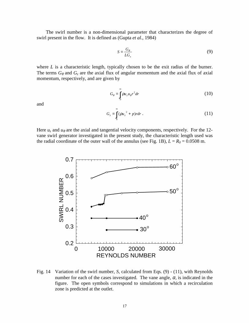
The swirl number is a non-dimensional parameter that characterizes the degree ofswirl present in the flow. It is defined as (Gupta et al., 1984)

zLGGS θ= (9)

where L is a characteristic length, typically chosen to be the exit radius of the burner.The terms Gθ and Gz are the axial flux of angular momentum and the axial flux of axialmomentum, respectively, and are given by

∫∞

=0

2drruuG z θθ ρ (10)

and

∫∞

+=0

2 )( rdrpuG zz ρ . (11)

Here uz and uθ are the axial and tangential velocity components, respectively. For the 12-vane swirl generator investigated in the present study, the characteristic length used wasthe radial coordinate of the outer wall of the annulus (see Fig. 1B), L = R0 = 0.0508 m.

0.2

0.3

0.4

0.5

0.6

0.7

0 10000 20000 30000REYNOLDS NUMBER

30o

40o

50o

60o

SWIR

L N

UM

BER

Fig. 14 Variation of the swirl number, S, calculated from Eqs. (9) - (11), with Reynoldsnumber for each of the cases investigated. The vane angle, α, is indicated in thefigure. The open symbols correspond to simulations in which a recirculationzone is predicted at the outlet.

18

Figure 14 presents the swirl number calculated at the outlet of the computationaldomain for each of the simulations in Table 1. The open symbols correspond to cases inwhich a recirculation zone was predicted at the outlet of the domain. For vane angles of30o and 40o, the swirl number is independent of Re over the range of Reynolds numbersinvestigated, indicating that viscosity effects are not significant. For these vane angles,simulations and correlations invoking the inviscid assumption will likely give reasonablepredictions. Note that the simulations corresponding to α = 30o or α = 40o do not predictthe presence of a recirculation zone at the outlet of the domain. For the simulations withvane angles of 50o and 60o, the swirl number is a weak function of Reynolds number, butreaches asymptotic values for high Reynolds numbers.

10-5

10-4

10-3

10-2

10-1

0 10000 20000 30000 40000REYNOLDS NUMBER

IPRESS

IAXIAL

ITANG

SU

RFA

CE

INTE

GR

AL

Fig. 15 Variation of the axial momentum (IAXIAL), tangential momentum (ITANG), andstatic pressure (IPRESS) contributions to the swirl number calculation withReynolds number.

The abrupt increase in the swirl number at Re ≈ 9,500 predicted for α = 50o

corresponds to the development of a recirculation zone at the outlet, and results from adecrease in the static pressure contribution in Eq. (11), as shown in Fig. 15. The curveslabeled IAXIAL, ITANG, and IPRESS in Fig. 15 correspond to

∫∞

=0

2rdruI zAXIAL ρ , (12)

19

∫∞

==0

2drruuGI zTANG θθ ρ , (13)

and

∫∞

=0

prdrI PRESS , (14)

respectively. The static pressure contribution to the swirl number, IPRESS, decreasesabruptly when the recirculation zone develops due to the negative static pressure in therecirculation zone. The decrease in IPRESS, which appears in the denominator of Eq. (9),results in an abrupt increase in the swirl number.

SummaryThe combustion air entering the reference spray combustion facility at NIST has

been investigated computationally using the Reynolds averaged Navier-Stokes equationsand the RNG k-ε turbulence model. The RNG k-ε turbulence model was previouslyvalidated experimentally for the confined, swirling flow studied in this investigation. Aparametric study is presented in which the effects of the Reynolds number and vane angleare examined for the ranges of 5,000 < Re < 30,000 and 30o < α < 60o. The simulationswith a vane angle of 50o, which is the current operating condition for the reference spraycombustion facility, predict the development of a recirculation zone for Re ≈ 9500. Thisreport completes a recent study intended to characterize the inlet combustion air in theNIST reference spray combustion facility. The details presented herein can be used asinlet conditions for modelers attempting to simulate the multiphase combustion processwithin the reactor.

AcknowledgementsThe authors would like to thank Mike Carrier for technical support. One of the

authors (JFW) wishes to acknowledge the financial support of the NRC/NISTPostdoctoral Research Program.

20

References

Benim, A. C. (1990). Finite Element Analysis of Confined Turbulent Swirling Flows.International Journal of Numerical Methods in Fluids. 11:697-717.

Bird, R. B., Stewart, W. E., and Lightfoot, E. N. (1960). Transport Phenomena, JohnWiley & Sons, New York.

Fluent 5 User's Guide. (1998). Fluent Incorporated, Lebanon, NH 03766 USA.

Gupta, A. K., Lilley, D. G., and Syred, N. (1984). Swirl Flows, Abacus Press, Kent.

Hinze, J. O. (1975). Turbulence, McGraw-Hill Publishing Co., New York.

Issa, R. I. (1986). Solution of Implicitly Discretized Fluid Flow Equations by OperatorSplitting. Journal of Computational Physics. 62:40-65.

Jaw, S. Y., and Chen, C. J. (1998). Present Status of Second-Order Closure TurbulenceModels. I: Overview. Journal of Engineering Mechanics. 124:485-501.

Launder, B. E., and Spalding, D. B. (1972). Lectures in Mathematical Models ofTurbulence, Academic Press, London.

Launder, B. E., and Spalding, D. B. (1974). The Numerical Computation of TurbulentFlows. Computer Methods in Applied Mechanics and Engineering. 3:269-289.

Lien, F. S., and Leschziner, M. A. (1994). Assessment of Turbulence-Transport ModelsIncluding Non-Linear RNG Eddy-Viscosity Formulation and Second-MomentClosure for Flow Over a Backward-Facing Step. Computers in Fluids. 23:983-1004.

Papageorgakis, G. C., and Assanis, D. N. (1999). Comparison of Linear and NonlinearRNG-Based k-ε Models for Incompressible Turbulent Flows. Numerical HeatTransfer, Part B. 35:1-22.

Sheen, H. J., Chen, W. J., and Wu, J. S. (1997). Flow Patterns for an Annular Flow Overan Axisymmetric Sudden Expansion. Journal of Fluid Mechanics. 350:177-188.

Shyy, W., Thakur, S. S., Ouyang, H., Liu, J., and Blosch, E. (1997). ComputationalTechniques for Complex Transport Phenomena. pp. 163-230. CambridgeUniversity Press, Cambridge, UK.

Smith, L. M., and Reynolds, W. C. (1992). On the Yakhot-Orszag RenormalizationGroup Method for Deriving Turbulence Statistics and Models. Physics of Fluids A,4:364-390.

21

Taylor, B. N., and Kuyatt, C. E. (1994). Guidelines for Evaluating and Expressing theUncertainty of NIST Measurement Results. NIST Technical Note 1297. NationalInstitute of Standards and Technology, Gaithersburg, MD, 20899.

Widmann, J. F., Charagundla, S. R., Presser, C., and Heckert, A. (1999a). BenchmarkExperimental Database for Multiphase Combustion Model Input and Validation:Baseline Case. NISTIR 6286. National Institute of Standards and Technology,Gaithersburg, MD 20899-8360, USA.

Widmann, J. F., Charagundla, S. R., and Presser, C. (1999b). Benchmark ExperimentalDatabase for Multiphase Combustion Model Input and Validation: Characterizationof the Inlet Combustion Air. NISTIR 6370. National Institute of Standards andTechnology, Gaithersburg, MD 20899-8360, USA.

Yakhot, V., and Orszag, S. A. (1986). Renormalization Group Analysis of Turbulence:I. Basic Theory. J. Scientific Computing, 1:1-51.

Yakhot, V., Orszag, S. A., Thangam, S., Gatski, T. B., and Speziale, C. G. (1992).Development of Turbulence Models for Shear Flows by a Double ExpansionTechnique. Physics of Fluids A. 4:1510-1520.

Yakhot, V., and Smith L. M. (1992). The Renormalization Group, the ε-Expansion andthe Derivation of Turbulence Models. Journal of Scientific Computing. 7:35-61.

Yin, M., Shi, F., and Xu, Z. (1996). Renormalization Group Based k-ε TurbulenceModel for Flows in a Duct with Strong Curvature. International Journal ofEngineering Science. 34:243-248.

characterization of the inlet combustion air in nist's ... characterization of the inlet...

Documents