characterization of the swelling properties of highly...
TRANSCRIPT

Technical Report Documentation Page
1. Report No. FHWA/TX-09/0-6048-1
2. Government Accession No.
3. Recipient’s Catalog No.
4. Title and Subtitle Characterization of the Swelling Properties of Highly Plastic Clays Using Centrifuge Technology
5. Report Date December 2008; Revised April 2009
6. Performing Organization Code 7. Author(s)
Jorge G. Zornberg, Jeffrey A. Kuhn, and Michael D. Plaisted 8. Performing Organization Report No.
0-6048-1
9. Performing Organization Name and Address Center for Transportation Research The University of Texas at Austin 3208 Red River, Suite 200 Austin, TX 78705-2650
10. Work Unit No. (TRAIS) 11. Contract or Grant No.
0-6048
12. Sponsoring Agency Name and Address Texas Department of Transportation Research and Technology Implementation Office P.O. Box 5080 Austin, TX 78763-5080
13. Type of Report and Period Covered Technical Report 09/2007–08/2008
14. Sponsoring Agency Code
15. Supplementary Notes Project performed in cooperation with the Texas Department of Transportation and the Federal Highway Administration.
16. Abstract A feasibility study was performed to determine the potential advantages of characterizing the swelling properties of highly plastic clay using a geotechnical centrifuge. This study consisted of an experimental program involving a series of tests in a small and large centrifuge in which water was ponded atop compacted clay specimens, flown up to speed, and the specimen’s height was monitored with time. This method allowed for the characterization of the swelling properties of the soil within 24 hours of the start of testing. Traditional free-swell testing to achieve the same level of characterization required approximately 30 days for the highly plastic clay evaluated in the study. This new centrifuge methodology for evaluating the swelling potential of clay was found to produce comparable results to traditional testing in a fraction of the time. Centrifuge testing of highly plastic clays will allow the Texas Department of Transportation to acquire a speedy characterization of the swelling characteristics of highly plastic clays by direct measurement of swelling rather than by the use of correlations between swelling and index properties or suction.
17. Key Words Highly plastic clay, swelling, and centrifugation,
18. Distribution Statement No restrictions. This document is available to the public through the National Technical Information Service, Springfield, Virginia 22161; www.ntis.gov.
19. Security Classif. (of report) Unclassified
20. Security Classif. (of this page) Unclassified
21. No. of pages 82
22. Price
Form DOT F 1700.7 (8-72) Reproduction of completed page authorized


Characterization of the Swelling Properties of Highly Plastic Clays Using Centrifuge Technology Jorge G. Zornberg, Ph.D., P.E. Jeffrey A. Kuhn Michael D. Plaisted CTR Technical Report: 0-6048-1 Report Date: December 2008; Revised April 2009 Project: 0-6048 Project Title: Soil Testing Using Centrifuge Technology Sponsoring Agency: Texas Department of Transportation Performing Agency: Center for Transportation Research at The University of Texas at Austin Project performed in cooperation with the Texas Department of Transportation and the Federal Highway Administration.

iv
Center for Transportation Research The University of Texas at Austin 3208 Red River Austin, TX 78705 www.utexas.edu/research/ctr Copyright (c) 2008 Center for Transportation Research The University of Texas at Austin All rights reserved Printed in the United States of America

v
Disclaimers Author's Disclaimer: The contents of this report reflect the views of the authors, who
are responsible for the facts and the accuracy of the data presented herein. The contents do not necessarily reflect the official view or policies of the Federal Highway Administration or the Texas Department of Transportation (TxDOT). This report does not constitute a standard, specification, or regulation.
Patent Disclaimer: There was no invention or discovery conceived or first actually reduced to practice in the course of or under this contract, including any art, method, process, machine manufacture, design or composition of matter, or any new useful improvement thereof, or any variety of plant, which is or may be patentable under the patent laws of the United States of America or any foreign country.
Engineering Disclaimer NOT INTENDED FOR CONSTRUCTION, BIDDING, OR PERMIT PURPOSES.
Project Engineer: Jorge G. Zornberg
Professional Engineer License State and Number: CA No. C 056325 P. E. Designation: Research Supervisor

vi
Acknowledgments The authors express appreciation for the dedicated guidance of the TxDOT Project
Director, Dr. Zhiming Si. We are also thankful for the input by members of the PMC, including David Head, Caroline Herrera, Christopher Weber, and Stanley Yin. RTI’s support by German Claros and Frank Espinosa is much valued.
vii
Table of Contents
Chapter 1. Introduction................................................................................................................ 1
Chapter 2. Assessment of Existing Information......................................................................... 3 2.1 TxDOT Research on Pavements over Expansive Clays ........................................................3 2.2 Conventional swelling tests on highly plastic clays ..............................................................4 2.3 The Potential Vertical Rise (PVR) Method ...........................................................................5 2.4 Potential Vertical Rise Revisited (TxDOT 0-4518) ..............................................................5 2.5 Infiltration tests on highly plastic clay in the centrifuge .......................................................7 2.6 Assessment of TxDOT needs ................................................................................................8
Chapter 3. Characterization of Eagle Ford Clay ....................................................................... 9 3.1 Index parameters ....................................................................................................................9
3.1.1 Grain size distribution .................................................................................................... 9 3.1.2 Atterberg limits .............................................................................................................. 9 3.1.3 Moisture density relationships ..................................................................................... 10 3.1.4 Specific gravity ............................................................................................................ 11
3.2 Free-swell tests ....................................................................................................................11 3.2.2 Effect of compaction water content on swelling .......................................................... 13 3.2.3 Effect of seating loads on swelling .............................................................................. 15 3.2.4 Findings from free-swell testing .................................................................................. 16
3.3 Saturated hydraulic conductivity .........................................................................................16 3.4 Summary of characterization of Eagle Ford Clay ...............................................................17
Chapter 4. Small Centrifuge Equipment and Procedure ........................................................ 19 4.1 Introduction ..........................................................................................................................19 4.2 Small Centrifuge Setup ........................................................................................................20
4.2.1 Centrifuge Cup ............................................................................................................. 20 4.2.2 Permeameter Cup ......................................................................................................... 20 4.2.3 Porous Supporting Plate ............................................................................................... 21 4.2.4 Permeameter Cap ......................................................................................................... 22
4.3 Small Centrifuge Testing Procedure ....................................................................................22 4.4 Small Centrifuge Typical Result and Repeatability ............................................................23
Chapter 5. Large Centrifuge Equipment and Procedure ....................................................... 25 5.1 Large Centrifuge Setup ........................................................................................................25
5.1.1 General Setup ............................................................................................................... 25 5.1.2 Permeameter Cup ......................................................................................................... 28 5.1.3 Permeameter Outflow Plate ......................................................................................... 29 5.1.4 Permeameter Cap and linear displacement transducer ................................................ 29 5.1.5 In-flight addition of water ............................................................................................ 30 5.1.6 Overview of the system ............................................................................................... 31
5.2 Large Centrifuge Testing Procedure ....................................................................................31 5.3 Typical test results ...............................................................................................................32 5.4 Key capabilities of the large centrifuge ...............................................................................34
viii
Chapter 6. Parametric Evaluation ............................................................................................ 35 6.1 Specimen Height ..................................................................................................................35 6.2 Water Head ..........................................................................................................................36 6.3 Overburden ..........................................................................................................................36 6.4 G-level .................................................................................................................................38
Chapter 7. Repeatability of Results in Large Centrifuge Testing .......................................... 39
Chapter 8. Comparison of Small and Large Centrifuge Test Results ................................... 41
Chapter 9. Comparison between 1G and nG Tests ................................................................. 43 9.1 Determining Effective Stress in the Centrifuge ...................................................................43
9.1.1 Accounting for Varied G-level .................................................................................... 43 9.1.2 Effect of Varying Hydraulic Conductivity................................................................... 44 9.1.3 Selection of Pore Water Pressure Profiles ................................................................... 48
9.2 Validation of Ng Results from 1g Relation .........................................................................49 9.3 Determining Stress-Strain Relation from Ng Tests .............................................................52
Chapter 10. Conclusions ............................................................................................................. 55
References .................................................................................................................................... 57
Appendix A: Small Centrifuge Testing Procedure .................................................................. 59
Appendix B: Large Centrifuge Testing Procedure .................................................................. 65

ix
List of Figures Figure 1.1: Centrifuge Testing Setup .............................................................................................. 1
Figure 2.1: (a) Logitudinal crack caused by volumetric changes induced by expansive clays; (b) Pavement constructed using geogrid reinforcements to prevent the development of logitudinal cracks induced by expansive clays ......................................... 4
Figure 2.2: Fixed-Ring Consolidation Cell (Olson, 2007) ............................................................. 5
Figure 2.3: Schematic of laboratory setup for diffusion experiment (pg. 43 of V.2) ..................... 7
Figure 2.4: Suction log time plot for determination of the diffusion coefficient α (pg. 60 of V.2) ................................................................................................................................. 7
Figure 2.5: Advancement of a wetting front in a highly plastic clay in a centrifuge, Frydman (1990) .................................................................................................................. 8
Figure 3.1: Grain size distribution for Eagle Ford Shale ................................................................ 9
Figure 3.2: Standard and Modified Proctor compaction curves for Eagle Ford Shale. ................ 10
Figure 3.3: Odeometer apparatus used in free-swell testing ......................................................... 11
Figure 3.4: Free-swell testing setup .............................................................................................. 12
Figure 3.5: Free-swell test on Eagle Ford clay ............................................................................. 13
Figure 3.6: Swell tests on compacted Eagle Ford clay specimens prepared at different water contents ................................................................................................................... 14
Figure 3.7: Results of swell testing on compacted Eagle Ford clay specimens at different water contents ................................................................................................................... 14
Figure 3.8: Swell tests on compacted Eagle Ford clay specimens subjected to different seating loads ...................................................................................................................... 15
Figure 3.9: Results of swell tests on compacted Eagle Ford clay specimens subjected to different seating loads ....................................................................................................... 16
Figure 3.10: Flexible-wall hydraulic conductivity test ................................................................. 17
Figure 4.1: View of the small centrifuge permeameter available at The University of Texas at Austin for the characterization of moisture movement through soils: ............... 19
Figure 4.2: Centrifuge cup ............................................................................................................ 20
Figure 4.3: Permeameter cup with base removed ......................................................................... 21
Figure 4.4: Porous supporting plate .............................................................................................. 21
Figure 4.5: Permeameter cap ........................................................................................................ 22
Figure 4.6: Illustration of L1 (Step 8) ........................................................................................... 22
Figure 4.7: Typical Small Centrifuge Test Set ............................................................................. 23
Figure 5.1: Large centrifuge permeameter .................................................................................... 26
Figure 5.2: Large centrifuge permeameter .................................................................................... 28
Figure 5.3: Acrylic permeameter cup for the large centrifuge ...................................................... 29
Figure 5.4: Base porous stone and outflow plate .......................................................................... 29
Figure 5.5: (a) Permeameter top cap (b) Linear position sensor ................................................... 30

x
Figure 5.6: Linear position sensor ................................................................................................ 30
Figure 5.7: Overview of centrifuge permeameter ......................................................................... 31
Figure 5.8: Initial large centrifuge testing results ......................................................................... 33
Figure 5.9: Outflow results from initial large centrifuge test ....................................................... 33
Figure 5.10: Typical results from large centrifuge testing using the a linear position sensor ................................................................................................................................ 34
Figure 6.1: Effect of sample heights on measured swell (200G with 2cm water head) ............... 35
Figure 6.2: Effect of water head on measured swell (3cm sample at 200G) ................................ 36
Figure 6.3: Stress Ranges Without Overburden ........................................................................... 37
Figure 6.4: Stress Ranges With Overburden................................................................................. 37
Figure 6.5: Effect of G-levels on measured swell (3cm sample with 2cm water head) ............... 38
Figure 7.1: Three large centrifuge tests performed at 200 G with 2 cm of soil and 1 cm of water .................................................................................................................................. 39
Figure 8.1: Comparison of small and large centrifuge results ...................................................... 41
Figure 8.2: Composite curve for small and large centrifuge tests ................................................ 42
Figure 9.1: Pore water pressures assuming constant and varied g-level ....................................... 44
Figure 9.2: Pressure heads, constant hydraulic conductivity. (1cm sample, 400g, 2cm water) ................................................................................................................................ 46
Figure 9.3: Pressure heads, one order of magnitude change in hydraulic conductivity. (1cm sample, 400g, 2cm water) ........................................................................................ 47
Figure 9.4: Pressure heads, two orders of magnitude change in hydraulic conductivity. (1cm sample, 400g, 2cm water) ........................................................................................ 47
Figure 9.5: Pressure heads, four orders of magnitude change in hydraulic conductivity. (1cm sample, 400g, 2cm water) ........................................................................................ 48
Figure 9.6: Simplified Pore Water Pressure Distributions............................................................ 49
Figure 9.7: Calculated Swell vs. Measured (varied PWPs) .......................................................... 50
Figure 9.8: Calculated Swell vs. Measured (corrected) ................................................................ 51
Figure 9.9: 1g best fit vs. Ng best fit............................................................................................. 52
Figure 9.10: Ng predicted vs. measured. ...................................................................................... 53
xi
List of Tables Table 3.1: Index properties of Eagle Ford Shale .......................................................................... 10
Table 4.1: Statistics of Repeatability Set ...................................................................................... 23
Table 5.1: Comparison of centrifuge environments for hydraulic characterization of soils ........ 27
Table 7.1: Variation in swell between tests for repeatability ........................................................ 39
Table 8.1: Comparison of small and large centrifuge test results ................................................. 42
Table 9.1: Test Set Data ................................................................................................................ 51

xii
1
Chapter 1. Introduction
The need to design and construct roadways on highly plastic clays is common in central and eastern Texas, where expansive clays are prevalent. Roadways constructed on highly plastic clay subgrades may be damaged as the result of significant volume changes that occur when such soils undergo cycles of wetting and drying. These volume changes induce vertical movements, accelerate the degradation of pavement materials, and ultimately shorten the service life of the roadway. Proper characterization of expansive clays is required for design of and remediation of roadways constructed on poor subgrade materials. Current methods for characterization of expansive clays, however, either do not properly replicate field conditions, require excessive time for testing, or require the measurement of index properties rather than the direct measurement of swelling. An alternative method is proposed in this study, involving the infiltration of water into highly plastic clays under an increased gravity field in a centrifuge. This will accelerate the infiltration process and, ultimately, the characterization of the expansive clay.
The University of Texas at Austin acquired a state-of-the-art centrifuge permeameter under the direction of Dr. Zornberg in the summer of 2006. This centrifuge permeameter equipment was developed to alleviate shortcomings in available techniques for the characterization of the hydraulic properties of soils. This centrifuge permeameter allows measurement of the variables relevant for characterization of highly plastic clays in an expedited fashion by allowing in-flight, continuous, data acquisition. Most importantly, centrifuge technology will facilitate the use of direct experimental measurement of the swelling of highly plastic clays, rather than the use of correlations based on index properties, as this has not been the common practice in the past due to time constraints in current experimental methods.
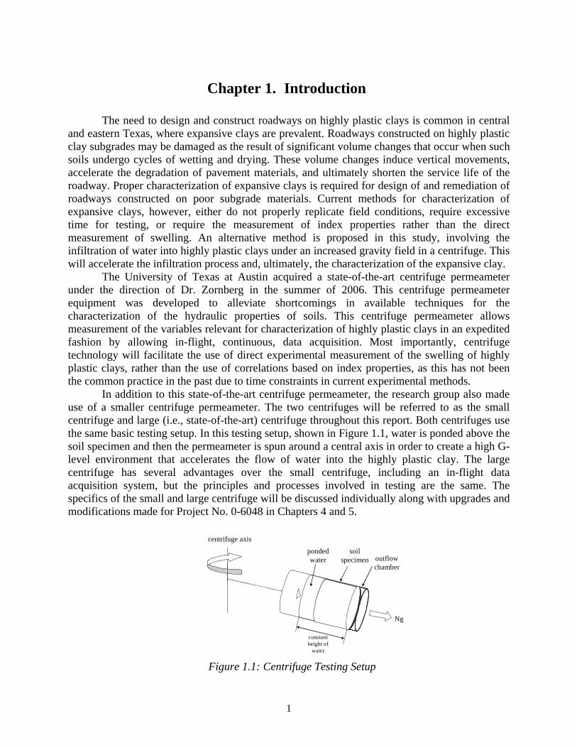
In addition to this state-of-the-art centrifuge permeameter, the research group also made use of a smaller centrifuge permeameter. The two centrifuges will be referred to as the small centrifuge and large (i.e., state-of-the-art) centrifuge throughout this report. Both centrifuges use the same basic testing setup. In this testing setup, shown in Figure 1.1, water is ponded above the soil specimen and then the permeameter is spun around a central axis in order to create a high G-level environment that accelerates the flow of water into the highly plastic clay. The large centrifuge has several advantages over the small centrifuge, including an in-flight data acquisition system, but the principles and processes involved in testing are the same. The specifics of the small and large centrifuge will be discussed individually along with upgrades and modifications made for Project No. 0-6048 in Chapters 4 and 5.
Figure 1.1: Centrifuge Testing Setup
centrifuge axis
outflow chamber
soil specimen
ponded water
constant height of
water
Ng

2

3
Chapter 2. Assessment of Existing Information
Literature concerning the simultaneous measurement of infiltration and swelling of highly plastic clays is scarce. The scarcity of literature on this subject is largely due to the extensive testing times required for testing volume changes in highly plastic clays using traditional laboratory methods. The extensive testing time required for traditional laboratory methods is demonstrated in section 3.2 where it is shown that a free-swell test on highly plastic clays took one month to run. The centrifuge technology presented in this report, however, shows that tests run in the centrifuge can be completed within one day.
In this assessment of existing information the following subjects will be covered: (1) Conventional swelling tests on highly plastic clays, (2) Benefits and disadvantages of conventional infiltration tests on highly plastic clays, (3) Infiltration tests on highly plastic clay in the centrifuge, (4) Swelling tests on highly plastic clay in the centrifuge, and (5) Assessment of TxDOT needs.
2.1 TxDOT Research on Pavements over Expansive Clays TxDOT has been actively investigating methods to quantify volumetric changes in
expansive clays as well as engineering solutions to address the problems posed by these volumetric changes in pavement design. The most common method used to predict vertical movements in highly plastic clays is the Potential Vertical Rise (PVR) method. The basis for the PVR method was developed by Chester McDowell (1956) and has been widely used with little revision since its inception. The methodology proposed by McDowell is based on a correlation between the plasticity index (PI) of the soil and the percent volumetric change. Once the plasticity index of a soil is measured, the percent volumetric change is then predicted for the overburden pressure at incremental depths within the soil profile of interest. The potential volumetric change is finally converted into a potential vertical rise for each layer and summed for the vertical profile in order to determine the total potential vertical rise. The PVR method, unfortunately, has often led to over-prediction of vertical movements. An additional drawback of the PVR method is that there has only been limited validation of the estimated potential vertical rise against movements measured in the field.
The PVR method was recently revisited by Lytton et al. (2005), who proposed a model for moisture movement based on a diffusion analysis and a previously developed model for volume changes based on changes in suction (Covar and Lytton 2001). In this updated PVR method, the diffusion analysis is used to predict changes in suction across time and space and subsequently volumetric changes in the soil across time and space. In order for a design engineer to make these calculations, a computer program was developed to calculate vertical movements based on a set of input parameters. Execution of this program requires environmental and geometric inputs, soil profile information, barrier and wheel path information, structural properties of the pavement, traffic information, reliability, and roadway roughness. One issue with the updated PVR method is that it is based on measurements made during drying processes, which may cause potential problems associated with repeatability of the results.
The recent Project 0-5812 exemplifies the efforts of the Department to address the problems associated with expansive clays in pavement performance. Specifically, this project has been conducted under the supervision of Dr. Jorge Zornberg in order to quantify the benefits of using geogrid-reinforcement to mitigate problems associated with expansive clay subgrades. The

4
specific problem being investigated is the development of longitudinal cracks that may develop even before new roads have been opened to traffic. Figure 2.1(a) illustrates the development of longitudinal cracks in a pavement constructed in Bryan District over expansive clays (FM 1915 in Milam County). The enhanced performance achieved by using geogrid reinforcements to mitigate this problem is shown in Figure 2.1(b) where it is evident that no longitudinal cracks have developed in the same road when the pavement incorporated the use of geogrid reinforcements.
While it appears that good engineering approaches are being developed to mitigate the problems associated with expansive clays, the proper characterization of the expansive clays is imperative in order to select the appropriate approach, and to conduct the subsequent pavement design. Expansive clays can be found across the entire state of Texas. These areas include Dallas, Fort Worth, Waco, Austin, San Antonio, Houston, El Paso, and numerous other areas. Jones and Holtz (1973) have estimated annual losses in the U.S. in excess of $2 billion due to expansive clays. Accordingly, the development of an accurate and expeditious method for characterization of expansive clays such as the one proposed in this study is expected lead to significant benefits to the Texas Department of Transportation.
Figure 2.1: (a) Logitudinal crack caused by volumetric changes induced by expansive clays;
(b) Pavement constructed using geogrid reinforcements to prevent the development of logitudinal cracks induced by expansive clays
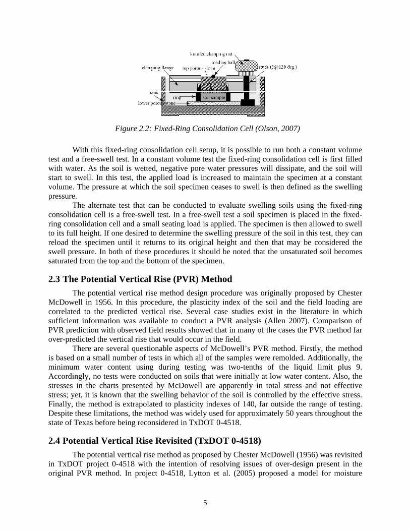
2.2 Conventional swelling tests on highly plastic clays Traditional swelling tests on highly plastic clay have been performed in a one-
dimensional odometer that is used in incremental vertical-flow consolidation (Figure 2.2). In this case, a specimen is placed into a ring and sandwiched between two porous stones that are protected from clogging by filter paper. The ring is held into a water tank by a clamping flange secured with a series of knurled clamping nuts. Finally, a load is placed on the top porous stone to confine the soil specimen.
5
Figure 2.2: Fixed-Ring Consolidation Cell (Olson, 2007)
With this fixed-ring consolidation cell setup, it is possible to run both a constant volume test and a free-swell test. In a constant volume test the fixed-ring consolidation cell is first filled with water. As the soil is wetted, negative pore water pressures will dissipate, and the soil will start to swell. In this test, the applied load is increased to maintain the specimen at a constant volume. The pressure at which the soil specimen ceases to swell is then defined as the swelling pressure.
The alternate test that can be conducted to evaluate swelling soils using the fixed-ring consolidation cell is a free-swell test. In a free-swell test a soil specimen is placed in the fixed-ring consolidation cell and a small seating load is applied. The specimen is then allowed to swell to its full height. If one desired to determine the swelling pressure of the soil in this test, they can reload the specimen until it returns to its original height and then that may be considered the swell pressure. In both of these procedures it should be noted that the unsaturated soil becomes saturated from the top and the bottom of the specimen.
2.3 The Potential Vertical Rise (PVR) Method The potential vertical rise method design procedure was originally proposed by Chester
McDowell in 1956. In this procedure, the plasticity index of the soil and the field loading are correlated to the predicted vertical rise. Several case studies exist in the literature in which sufficient information was available to conduct a PVR analysis (Allen 2007). Comparison of PVR prediction with observed field results showed that in many of the cases the PVR method far over-predicted the vertical rise that would occur in the field.
There are several questionable aspects of McDowell’s PVR method. Firstly, the method is based on a small number of tests in which all of the samples were remolded. Additionally, the minimum water content using during testing was two-tenths of the liquid limit plus 9. Accordingly, no tests were conducted on soils that were initially at low water content. Also, the stresses in the charts presented by McDowell are apparently in total stress and not effective stress; yet, it is known that the swelling behavior of the soil is controlled by the effective stress. Finally, the method is extrapolated to plasticity indexes of 140, far outside the range of testing. Despite these limitations, the method was widely used for approximately 50 years throughout the state of Texas before being reconsidered in TxDOT 0-4518.
2.4 Potential Vertical Rise Revisited (TxDOT 0-4518) The potential vertical rise method as proposed by Chester McDowell (1956) was revisited
in TxDOT project 0-4518 with the intention of resolving issues of over-design present in the original PVR method. In project 0-4518, Lytton et al. (2005) proposed a model for moisture

6
movement based on a diffusion analysis and a model for volume changed based on change in suction. The project reviewed the basic assumptions of the existing PVR methodology and suggested an alternative procedure for evaluating PVR.
In this revised PVR methodology, an evaporation experiment is conducted in order to determine the diffusion coefficient of a soil. The diffusion analysis was then used to predict special changes in suction with time. Based on modeled spatial changes in suction, volumetric changes in the soil are calculated for one-dimensional profiles of soil and the potential vertical rise is estimated.
Lytton et al. (2005) developed a computer program, WINPRES, to complement implementation of their research. In the computer program, the following inputs are required: environmental and geometric information, soil profile information, barrier and wheel path information, structural properties of the pavement, traffic information, reliability, and roadway roughness. The program outputs predictions of vertical movements, suction profiles, and roughness with time.
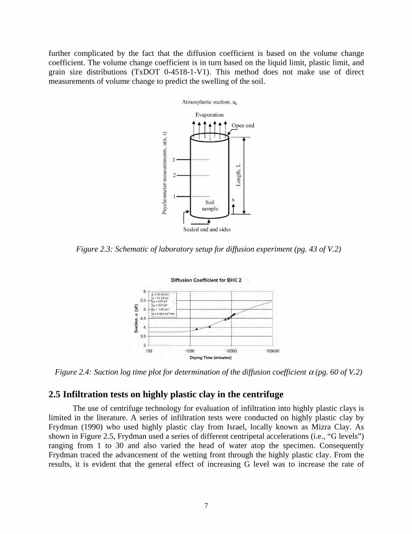
A new laboratory procedure was proposed as part of this project in order to estimate the diffusion coefficient. The setup of the diffusion experiment used to determine a diffusion coefficient, α, is shown in Figure 2.3. A specimen of highly plastic clay is first extracted from a Shelby tube. Holes are then drilled along its length for the placement of thermocouple psychrometers. The specimen is then wrapped in aluminum foil and placed inside of Styrofoam in a vertical tube with one end sealed. Finally, the specimen is placed in a temperature-controlled environment with the sealed end facing down and suction is monitored along the soil specimen’s length as evaporation occurs from the open end of the specimen. The experiment is analyzed by first plotting the soil suctions measured during the experiment versus the log of time as shown in Figure 2.4. Then, the suctions values at the boundaries and the geometry of the soil specimen are used in a MATLAB program written by the researchers (alphadrytest and drytest). Finally, an α coefficient is determined by fitting the diffusion relationship to the laboratory data. Finally the authors ask for the soil diffusion coefficient to be reported to the nearest seven decimal places. The authors do not justify why such accuracy is necessary.
As shown in the suction versus time data plotted in Figure 2.4, data are only plotted for times between 1,000 and 10,000 minutes. It is unclear as to why data is not plotted for smaller or larger times. Furthermore, the model does not appear to fit the observed data very well. For times greater than 10,000 minutes the predictive relationship indicates that suction should continue to increase. In order to verify this curve fitting methodology and the resulting predictive relationship, suction records at larger times are needed.
As with any testing method, there are issues that arise with respect to the method’s ability to measure the variables of interest and the method’s repeatability. In the revisited version of the PVR method, an evaporation test is conducted in order to evaluate moisture movement. It should be noted that swelling occurs during a wetting process in the soil and that moisture movement during wetting and drying will differ substantially based on the hysteretic nature of the permeability of the soil. Furthermore, the method makes use of a diffusion coefficient. The use of a singular diffusion coefficient to express the rate of moisture movement simplifies the process of moisture movement. The diffusion coefficient is based on a simplification of Richard’s equation, which expresses the relationship between head gradients and flow through an unsaturated soil. This method also makes use of the slope of the soil water retention curve for determination of the α coefficient. As per the procedure the soil water retention curve is not necessarily measured and is instead determined from an empirical relationship. The model is
7
further complicated by the fact that the diffusion coefficient is based on the volume change coefficient. The volume change coefficient is in turn based on the liquid limit, plastic limit, and grain size distributions (TxDOT 0-4518-1-V1). This method does not make use of direct measurements of volume change to predict the swelling of the soil.
Figure 2.3: Schematic of laboratory setup for diffusion experiment (pg. 43 of V.2)
Figure 2.4: Suction log time plot for determination of the diffusion coefficient α (pg. 60 of V.2)
2.5 Infiltration tests on highly plastic clay in the centrifuge The use of centrifuge technology for evaluation of infiltration into highly plastic clays is
limited in the literature. A series of infiltration tests were conducted on highly plastic clay by Frydman (1990) who used highly plastic clay from Israel, locally known as Mizra Clay. As shown in Figure 2.5, Frydman used a series of different centripetal accelerations (i.e., “G levels”) ranging from 1 to 30 and also varied the head of water atop the specimen. Consequently Frydman traced the advancement of the wetting front through the highly plastic clay. From the results, it is evident that the general effect of increasing G level was to increase the rate of

8
advancement of the wetting front. It should also be noted that a higher head atop the specimen lead to a faster advancement of the wetting front.
Figure 2.5: Advancement of a wetting front in a highly plastic clay in a centrifuge, Frydman (1990)
Use of centrifuge technology for characterization of volumetric changes in highly plastic clay is not well documented in the literature. In the aforementioned infiltration experiments conducted by Frydman, infiltration into highly plastic clay was performed in the centrifuge, but vertical swelling was not monitored. Several papers including Robinson et al. (2003) and Lee and Fox (2005) report on seepage consolidation in the centrifuge, but do not go into swelling measurements in the centrifuge. Another paper by Mitchell (1995) details the use of centrifuge testing for clay liner samples but again does not go into swelling measurements in the centrifuge.
2.6 Assessment of TxDOT needs TxDOT would benefit from a methodology that can be used to characterize the swelling
of highly plastic clay under conditions representative of those in the field. The tests need to directly measure the swelling of the soil and should avoid any predictive correlations for predicting swelling. This test should be able to be conducted in a reasonably short amount of time and the results of the test should be reproducible. The ability to conduct tests within a short time period will allow multiple tests to be run on a soil of interest. These tests can be related to local index properties for that soil group or specific project which may have the potential to be used for predicting swelling. Centrifuge testing of highly plastic soils allows for the direct measurement of vertical swelling in tests that can be conducted within a short time period. Furthermore, centrifuge testing of swelling soils provides the assurance that the full amount of swelling has occurred during testing in that time of equilibrium are able to be reached. On the other hand, testing under normal gravity leads to tests that may need to be suspended before having reached steady-state.
9
Chapter 3. Characterization of Eagle Ford Clay
3.1 Index parameters The highly plastic clay selected for this study was excavated from the Eagle Ford
formation in Round Rock, Texas. Clay from the Eagle Ford formation was selected for this study because it is known to generally have a high swelling potential. The Eagle Ford clay attained for this research study was excavated at the site from a depth of 10 feet with a backhoe. The color of excavated soil was mostly gray with yellow coloring. Prior to testing, the soil was air-dried, crushed, and processed. After being air-dried and processed, the soil appeared tan in color. The soil was dried at a temperature of approximately 120°F, not exceeding 140°F, according to ASTM D 698-00a so that changes in the soil properties would not occur. The following tests were performed to provide index parameters for the soil: grain size distribution; Atterberg limits; moisture density relationships; and specific gravity.
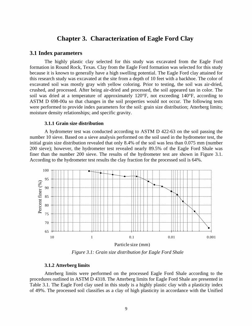
3.1.1 Grain size distribution A hydrometer test was conducted according to ASTM D 422-63 on the soil passing the
number 10 sieve. Based on a sieve analysis performed on the soil used in the hydrometer test, the initial grain size distribution revealed that only 8.4% of the soil was less than 0.075 mm (number 200 sieve); however, the hydrometer test revealed nearly 89.5% of the Eagle Ford Shale was finer than the number 200 sieve. The results of the hydrometer test are shown in Figure 3.1. According to the hydrometer test results the clay fraction for the processed soil is 64%.
Figure 3.1: Grain size distribution for Eagle Ford Shale
3.1.2 Atterberg limits Atterberg limits were performed on the processed Eagle Ford Shale according to the
procedures outlined in ASTM D 4318. The Atterberg limits for Eagle Ford Shale are presented in Table 3.1. The Eagle Ford clay used in this study is a highly plastic clay with a plasticity index of 49%. The processed soil classifies as a clay of high plasticity in accordance with the Unified
65
70
75
80
85
90
95
100
0.0010.010.1110
Perc
ent f
iner
(%)
Particle size (mm)
10
Soil Classification system. Given the clay fraction of 64% and the Atterberg limits, the activity of the soil is 0.77.
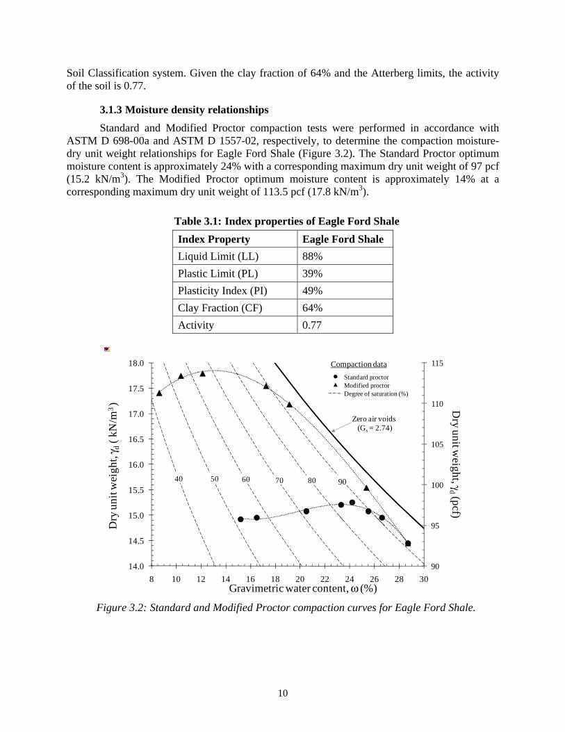
3.1.3 Moisture density relationships Standard and Modified Proctor compaction tests were performed in accordance with
ASTM D 698-00a and ASTM D 1557-02, respectively, to determine the compaction moisture-dry unit weight relationships for Eagle Ford Shale (Figure 3.2). The Standard Proctor optimum moisture content is approximately 24% with a corresponding maximum dry unit weight of 97 pcf (15.2 kN/m3). The Modified Proctor optimum moisture content is approximately 14% at a corresponding maximum dry unit weight of 113.5 pcf (17.8 kN/m3).
Table 3.1: Index properties of Eagle Ford Shale Index Property Eagle Ford Shale Liquid Limit (LL) 88% Plastic Limit (PL) 39% Plasticity Index (PI) 49% Clay Fraction (CF) 64% Activity 0.77
Figure 3.2: Standard and Modified Proctor compaction curves for Eagle Ford Shale.
90
95
100
105
110
115
14.0
14.5
15.0
15.5
16.0
16.5
17.0
17.5
18.0
8 10 12 14 16 18 20 22 24 26 28 30
Dry unit w
eight, γd (pcf)D
ry u
nit w
eigh
t, γ d
( kN
/m3 )
Gravimetric water content, ω (%)
Standard proctorModified proctorDegree of saturation (%)
90807060
Compaction data
Zero air voids (Gs = 2.74)
5040

11
3.1.4 Specific gravity Two specific gravity measurements were performed on the fraction of soil passing the
No. 4 sieve in accordance with ASTM D 854-02. The specific gravity values from the two measurements were 2.731 and 2.742 for an average value of 2.74.
3.2 Free-swell tests A series of baseline free-swell tests were conducted on a specimen of Eagle Ford clay
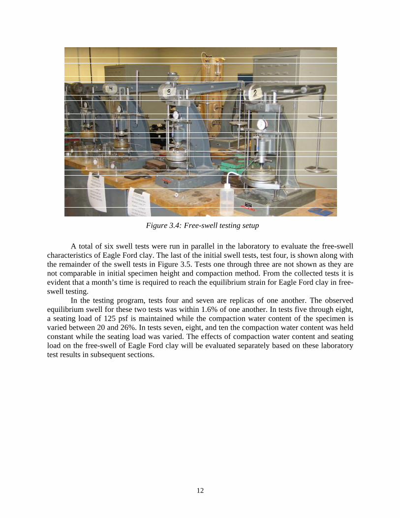
compacted at optimum water content and to a density equivalent to 100% of standard proctor compaction. The apparatus used for free-swell testing is the odeometer pictured in Figure 3.3. The soil specimen is placed in a fixed-ring consolidation cell as described in Section 2.2, and the specimen is subjected to a confining pressure. During testing, vertical movements of the specimen were monitored with a dial gauge and a linear variable differential transducer (LVDT). After the specimen is placed in the apparatus and then seating load is applied, the height of the specimen is monitored. Once the height of the specimen comes to equilibrium, data is logged from the LVDT and water is added to the reservoir in which the soil specimen is sitting in order to begin swell testing of the specimen. Based on the experience of the initial three tests conducted to investigate the free-swell properties of Eagle-Ford clay, it was expected to take approximately one month for specimens to swell to their full height. This height of the specimen at this last stage is termed the “equilibrium swell height.” Because the tests are long in duration, a series of swell tests were run in parallel in the laboratory (Figure 3.4).
Figure 3.3: Odeometer apparatus used in free-swell testing
Nominal weight
Dial gauge
Linear variableDisplacement transducer
Soil specimen in consolidation ring
12
Figure 3.4: Free-swell testing setup
A total of six swell tests were run in parallel in the laboratory to evaluate the free-swell characteristics of Eagle Ford clay. The last of the initial swell tests, test four, is shown along with the remainder of the swell tests in Figure 3.5. Tests one through three are not shown as they are not comparable in initial specimen height and compaction method. From the collected tests it is evident that a month’s time is required to reach the equilibrium strain for Eagle Ford clay in free-swell testing.
In the testing program, tests four and seven are replicas of one another. The observed equilibrium swell for these two tests was within 1.6% of one another. In tests five through eight, a seating load of 125 psf is maintained while the compaction water content of the specimen is varied between 20 and 26%. In tests seven, eight, and ten the compaction water content was held constant while the seating load was varied. The effects of compaction water content and seating load on the free-swell of Eagle Ford clay will be evaluated separately based on these laboratory test results in subsequent sections.
13
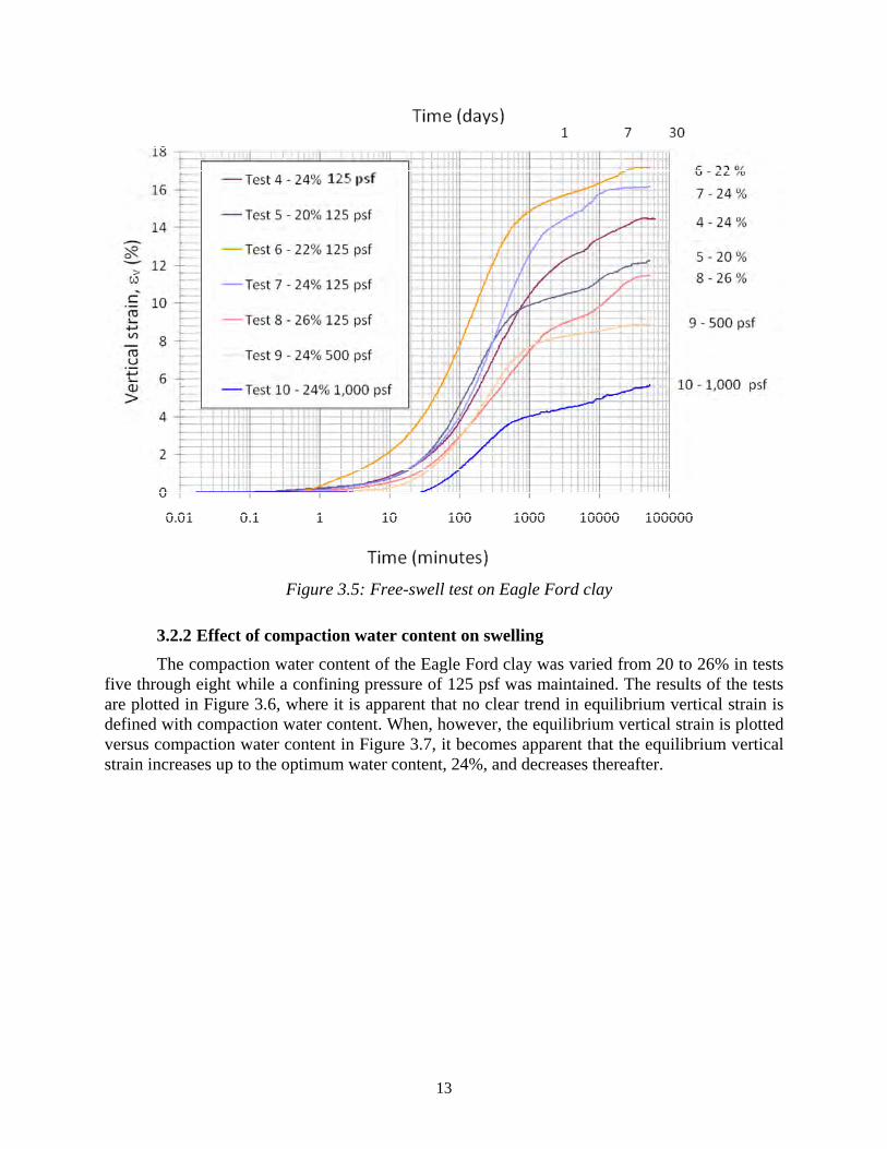
Figure 3.5: Free-swell test on Eagle Ford clay
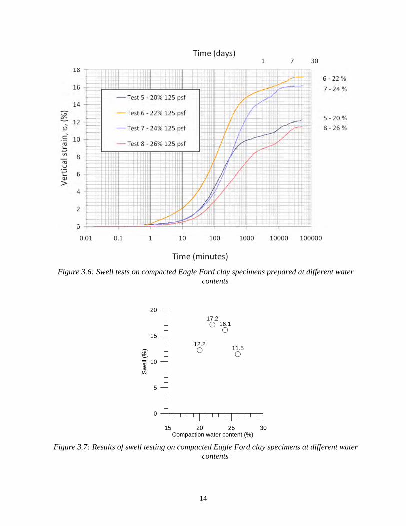
3.2.2 Effect of compaction water content on swelling The compaction water content of the Eagle Ford clay was varied from 20 to 26% in tests
five through eight while a confining pressure of 125 psf was maintained. The results of the tests are plotted in Figure 3.6, where it is apparent that no clear trend in equilibrium vertical strain is defined with compaction water content. When, however, the equilibrium vertical strain is plotted versus compaction water content in Figure 3.7, it becomes apparent that the equilibrium vertical strain increases up to the optimum water content, 24%, and decreases thereafter.
14
Figure 3.6: Swell tests on compacted Eagle Ford clay specimens prepared at different water
contents
Figure 3.7: Results of swell testing on compacted Eagle Ford clay specimens at different water
contents
15 20 25 30Compaction water content (%)
0
5
10
15
20
Sw
ell (
%)
12.2
17.216.1
11.5

15
3.2.3 Effect of seating loads on swelling In tests seven, eight, and ten the compaction water content was held constant at 24%
while the seating load was increased from the baseline value of 125 psf, to 500 psf, and finally 1,000 psf. The results of these tests are plotted together in Figure 3.8. The vertical strains observed in these three tests show a decrease in equilibrium vertical strain with increasing seating load. When the equilibrium strains for these three tests are plotted versus seating load in Figure 3.9, a log-linear relationship can be observed. This logarithmic relationship between equilibrium swell and seating load will be later used in modeling swelling behavior in the centrifuge.
Figure 3.8: Swell tests on compacted Eagle Ford clay specimens subjected to different seating
loads

16
Figure 3.9: Results of swell tests on compacted Eagle Ford clay specimens subjected to
different seating loads
3.2.4 Findings from free-swell testing The free-swell tests conducted on Eagle Ford clay allowed determination of the time to
equilibrium for free-swell test, the repeatability of free-swell tests, the effects of compaction water content on free-swell, and the effects of seating load on free-swell. A time period of one month was required for specimen to reach their final equilibrium strain. Two tests conducted under identical seating loads and compaction water content showed a difference of 1.6% between their equilibrium strains. The equilibrium swell was observed to increase in magnitude up to the optimum water content and decrease thereafter. The relationship between equilibrium swell and seating load was shown to be log-linear.
3.3 Saturated hydraulic conductivity The standard test method for evaluating the movement of water through a saturated
highly plastic clays is to measure the hydraulic conductivity of a saturated specimen in a flexible wall permeameter cell (Figure 3.10). For this test, Eagle Ford clay was compacted at a moisture content of approximately 23.6%, which is within 1% of optimum (24%), and a dry unit weight of 98.7 pcf (Γd,max = 97.5 pcf). The height-to-diameter ratio of this specimen was approximately 0.5. Because this clay is highly plastic and has a low hydraulic conductivity, the back-pressure saturation and consolidation of the specimen was time consuming. After saturation and consolidation at an effective stress of 4 psi, a hydraulic gradient of 20 was applied between the top and bottom of the specimen. The flow rate into and out of the specimen was then measured until the ratio of the outflow to inflow was at least 0.99. The hydraulic conductivity was found to be approximately 8 x 10⁻⁹ ft/min (4 x 10⁻⁹ cm/s).
100 1000Seating load (psf)
0
5
10
15
20
Sw
ell (
%)
16.1
8.9
5.7

17
Figure 3.10: Flexible-wall hydraulic conductivity test
3.4 Summary of characterization of Eagle Ford Clay Eagle Ford clay was found to be highly plastic with a plasticity index of 49. In the Eagle Ford clay, 97% of the particles were found to be clay-sized particles. The optimum water content for standard proctor compaction was 24%. Free-swell testing on Eagle Ford clay revealed a requisite testing time of 30 days and a log-linear relationship between equilibrium strain and seating load. The hydraulic conductivity of Eagle Ford clay at optimum water content and Standard Proctor compaction effort was found to be 4 x 10⁻⁹ cm/s.

18

19
Chapter 4. Small Centrifuge Equipment and Procedure
4.1 Introduction A state-of-the-art centrifuge laboratory has been recently added to the geotechnical
laboratories at The University of Texas at Austin. One of the available apparatus involves a small centrifuge that has been upgraded to house a permeameter (Figure 4.1a). The small centrifuge equipment is suitable for pilot tests that do not require the use of controlled influx and that do not require in-flight instrumentation. The testing setup for the small permeameter involves two components, as shown in Figure 4.1b. The first component is a permeameter cup that contains the soil specimen and the permeant (i.e., water). The soil specimen is compacted within the permeameter cup and is sandwiched between two porous plastic plates. Filter paper is used to separate the soil specimen from the porous plastic plates at each boundary. The porous plate at the upper boundary allows water to freely flow into the specimen. Another porous plate at the lower boundary allows water to freely flow out of the specimen. The second component of small centrifuge testing is a custom-made centrifuge cup. A more detailed description of each component is included in section 4.2. During centrifuge testing, the permeameter cup is placed in the centrifuge cup on top of the soil sample. The small centrifuge is capable of flying four permeameter cups simultaneously. The ability to test duplicate soil specimens in parallel in the centrifuge is a significant advantage as it allows evaluation of test repeatability.
Figure 4.1: View of the small centrifuge permeameter available at The University of Texas at
Austin for the characterization of moisture movement through soils: (a) view of the small centrifuge; (b) view of the permeameter. The small centrifuge equipment is
suitable for pilot tests that do not require the use of controlled influx and that do not need the use of in-flight instrumentation.
20
4.2 Small Centrifuge Setup The small centrifuge is a modified asphalt centrifuge with four arms that hold metallic
centrifuge cups. The setup of the centrifuge is fairly customizable as the contents of the centrifuge cups can be altered to fit requirements of different tests. Plastic permeameter cups that fit inside the centrifuge cups were designed and manufactured specifically for this project. The main components are discussed individually below.
4.2.1 Centrifuge Cup The centrifuge cups, which hang from the spinning centrifuge arms, were provided with
the centrifuge and have not been significantly altered (Figure 4.2). The holders have an inner diameter of 2.5 inches and a usable inside depth of 4.5 inches. The base of the specimen holder has a small vent hole to allow air and water outflow. When in flight the distance from the base of a sample and the center of rotation in the small centrifuge is approximately 6.5 inches.
Figure 4.2: Centrifuge cup
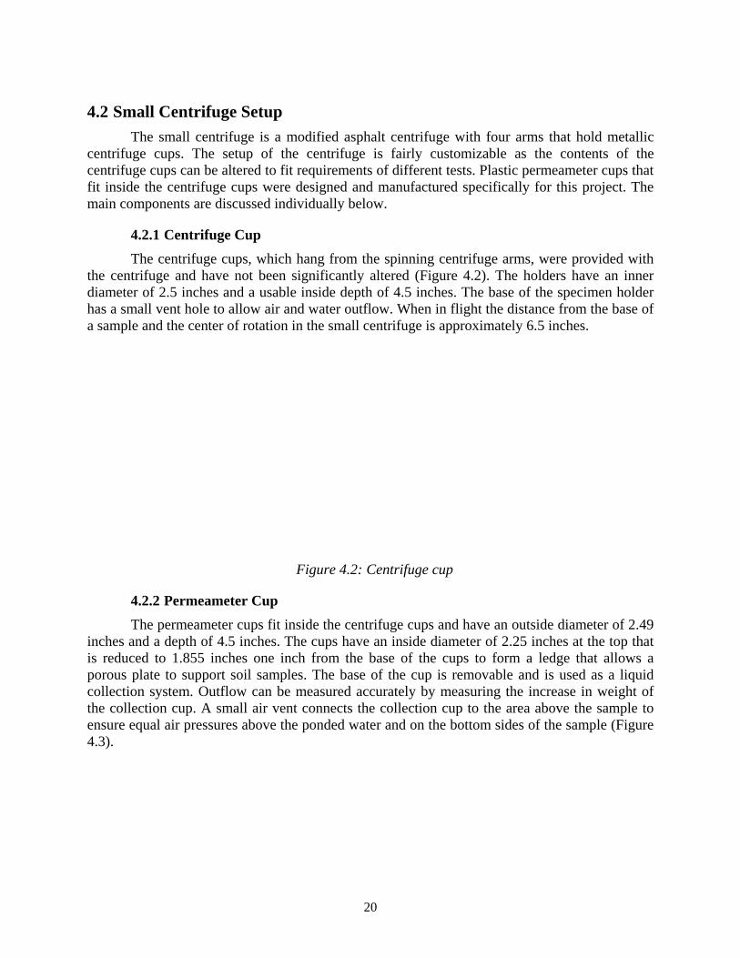
4.2.2 Permeameter Cup The permeameter cups fit inside the centrifuge cups and have an outside diameter of 2.49
inches and a depth of 4.5 inches. The cups have an inside diameter of 2.25 inches at the top that is reduced to 1.855 inches one inch from the base of the cups to form a ledge that allows a porous plate to support soil samples. The base of the cup is removable and is used as a liquid collection system. Outflow can be measured accurately by measuring the increase in weight of the collection cup. A small air vent connects the collection cup to the area above the sample to ensure equal air pressures above the ponded water and on the bottom sides of the sample (Figure 4.3).

21
Figure 4.3: Permeameter cup with base removed
4.2.3 Porous Supporting Plate The porous supporting plate seen in Figure 4.4 sits on top of the ledge in the permeameter
cup and creates a surface to place specimens. The plate contains 1/32” holes that allow water to flow freely from the base of the specimen. To avoid soil migration a filter paper is placed in between the porous plate and soil specimen.
Figure 4.4: Porous supporting plate
Air vent
Removable base
22
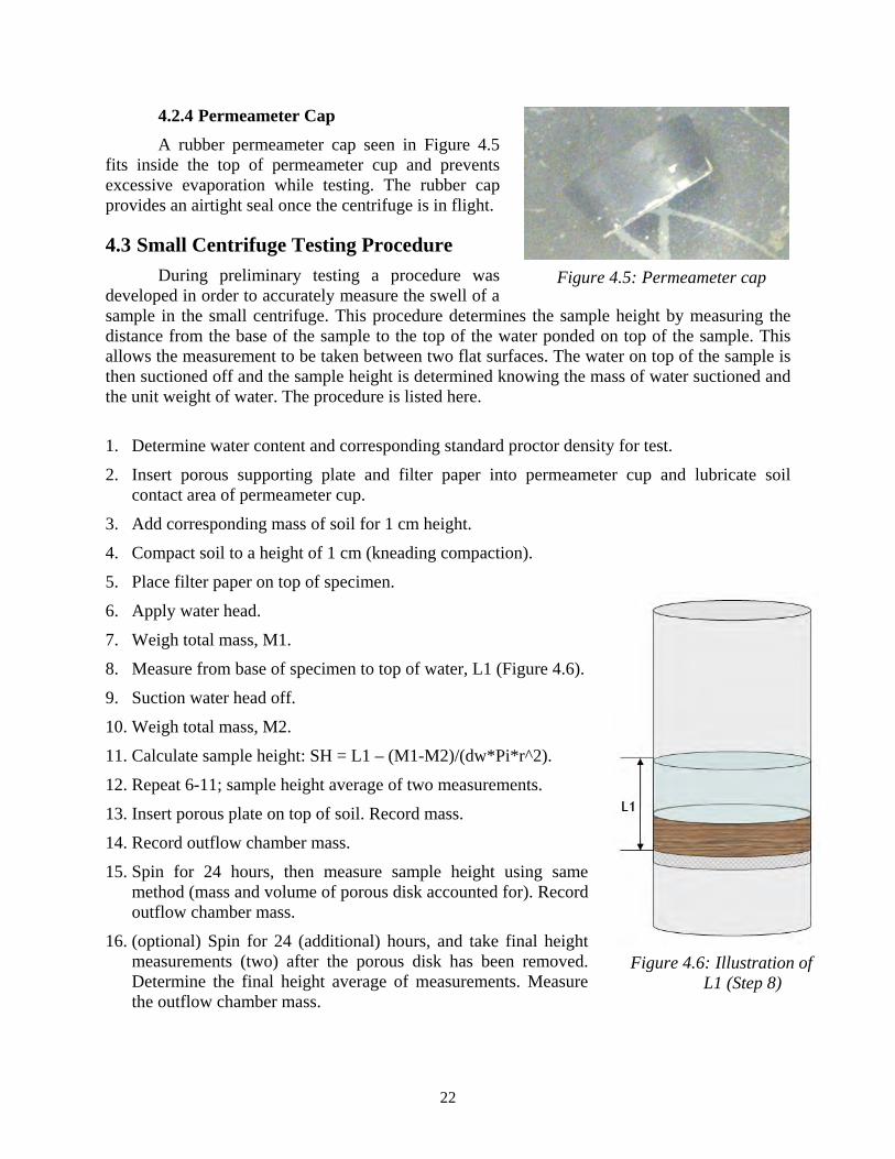
4.2.4 Permeameter Cap A rubber permeameter cap seen in Figure 4.5
fits inside the top of permeameter cup and prevents excessive evaporation while testing. The rubber cap provides an airtight seal once the centrifuge is in flight.
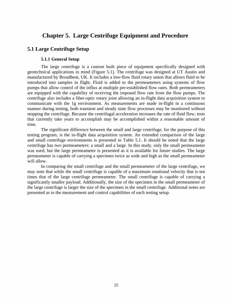
4.3 Small Centrifuge Testing Procedure During preliminary testing a procedure was
developed in order to accurately measure the swell of a sample in the small centrifuge. This procedure determines the sample height by measuring the distance from the base of the sample to the top of the water ponded on top of the sample. This allows the measurement to be taken between two flat surfaces. The water on top of the sample is then suctioned off and the sample height is determined knowing the mass of water suctioned and the unit weight of water. The procedure is listed here.
1. Determine water content and corresponding standard proctor density for test.
2. Insert porous supporting plate and filter paper into permeameter cup and lubricate soil contact area of permeameter cup.
3. Add corresponding mass of soil for 1 cm height.
4. Compact soil to a height of 1 cm (kneading compaction).
5. Place filter paper on top of specimen.
6. Apply water head.
7. Weigh total mass, M1.
8. Measure from base of specimen to top of water, L1 (Figure 4.6).
9. Suction water head off.
10. Weigh total mass, M2.
11. Calculate sample height: SH = L1 – (M1-M2)/(dw*Pi*r^2).
12. Repeat 6-11; sample height average of two measurements.
13. Insert porous plate on top of soil. Record mass.
14. Record outflow chamber mass.
15. Spin for 24 hours, then measure sample height using same method (mass and volume of porous disk accounted for). Record outflow chamber mass.
16. (optional) Spin for 24 (additional) hours, and take final height measurements (two) after the porous disk has been removed. Determine the final height average of measurements. Measure the outflow chamber mass.
Figure 4.5: Permeameter cap
Figure 4.6: Illustration of L1 (Step 8)

23
This procedure was used during testing and provided highly repeatable results. One major benefit of this procedure is that it eliminates the issues associated with measuring a non-uniform surface such as the top of the soil sample. By using the water surface as a reference point the average height of the non-uniform soil sample can accurately be determined.
4.4 Small Centrifuge Typical Result and Repeatability A series of tests were performed to evaluate the repeatability of the small centrifuge. Six
tests were run at a g-level of 400 with two centimeters of water head and 480 psf of overburden. The target sample height was one centimeter; however, the samples in this data set were slightly under-compacted and had an average height of 1.06 cm. The tests were run using the procedure discussed in section 4.3.
The six tests are graphed together in Figure 4.7. The final strains of the samples are very consistent at approximately 8% strain. Statistical data for these tests are provided in Table 4.1. These tests show the high repeatability of tests run in the small centrifuge. Most notable is the low standard deviation of the test set (i.e., less than 1% strain or .01cm).
Table 4.1: Statistics of Repeatability Set Average 7.90%Standard Deviation 0.86%Minimum 6.60%Maximum 9.03%
Figure 4.7: Typical Small Centrifuge Test Set
400g, WH=2cm, SH=1cm, 15g (480psf) OB
0%
2%
4%
6%
8%
10%
12%
0 5 10 15 20 25 30 35 40 45 50
Time (hrs)
Stra
in
Jul 14, SH=1.03
Jul 14, SH=1.07
Jul 12, SH=1.05
Jul 12, SH=1.08
Jul 10, SH=1.07
Jul 10, SH=1.07

24
25
Chapter 5. Large Centrifuge Equipment and Procedure
5.1 Large Centrifuge Setup
5.1.1 General Setup The large centrifuge is a custom built piece of equipment specifically designed with
geotechnical applications in mind (Figure 5.1). The centrifuge was designed at UT Austin and manufactured by Broadbent, UK. It includes a low-flow fluid rotary union that allows fluid to be introduced into samples in flight. Fluid is added to the permeameters using systems of flow pumps that allow control of the influx at multiple pre-established flow rates. Both permeameters are equipped with the capability of receiving the imposed flow rate from the flow pumps. The centrifuge also includes a fiber-optic rotary joint allowing an in-flight data acquisition system to communicate with the 1g environment. As measurements are made in-flight in a continuous manner during testing, both transient and steady state flow processes may be monitored without stopping the centrifuge. Because the centrifugal acceleration increases the rate of fluid flow, tests that currently take years to accomplish may be accomplished within a reasonable amount of time.
The significant difference between the small and large centrifuge, for the purpose of this testing program, is the in-flight data acquisition system. An extended comparison of the large and small centrifuge environments is presented in Table 5.1. It should be noted that the large centrifuge has two permeameters: a small and a large. In this study, only the small permeameter was used, but the large permeameter is presented as it is available for future studies. The large permeameter is capable of carrying a specimen twice as wide and high as the small permeameter will allow.
In comparing the small centrifuge and the small permeameter of the large centrifuge, we may note that while the small centrifuge is capable of a maximum rotational velocity that is ten times that of the large centrifuge permeameter. The small centrifuge is capable of carrying a significantly smaller payload. Additionally, the size of the specimen in the small permeameter of the large centrifuge is larger the size of the specimen in the small centrifuge. Additional notes are presented as to the measurement and control capabilities of each testing setup.

26
Figure 5.1: Large centrifuge permeameter

27
Table 5.1: Comparison of centrifuge environments for hydraulic characterization of soils
Small Centrifuge
Large centrifuge Small permeameter Large permeameter
Centrifuge details Maximum rotational
velocity (rpm) 10,000 900 900
Centrifuge arm to base of specimen (mm) 175 613 624
Maximum g-level at base of specimen 17,000 500 500
Permeameter details Diameter (mm) 57 71 153
Maximum specimen height (mm) 85 127 306
Measurement and control
capabilities Head of water on top of
specimen NA Addition of fluid through rotary joint
Addition of fluid through rotary joint
Flow rate into specimen NA Addition of fluid with
a infusion pump through a rotary joint
Addition of fluid with a infusion pump
through a rotary joint
Outflow volume
Test must be stopped, determined by weighting on a laboratory scale
In-flight via pressure transducer
In-flight via pressure transducer
Soil suction NA In-flight via heat dissipation units
In-flight via heat dissipation units
Volumetric water content NA
In-flight, bulk measurement via
vertical time domain reflectometry probe
In-flight, profile measurements via
horizontal time domain reflectometry
probes The permeameter cup varies from that used in the small centrifuge in that it has a larger
diameter (2.5 inches instead of 2.25) along with instrumentation that allows for real time, in-flight monitoring of sample height and outflow. The large centrifuge is very flexible and has previously measured things such as water content and suction also.
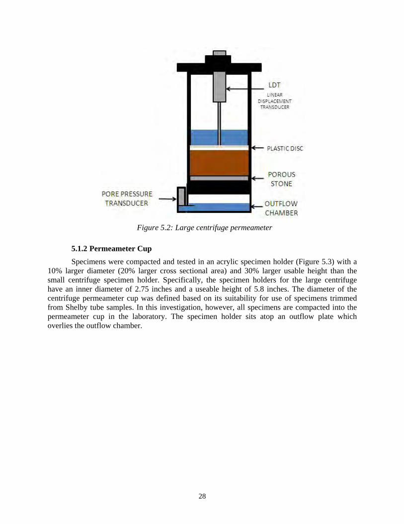
The large centrifuge permeameter consists of a permeameter cup, outflow plate, permeameter cap, and linear position sensor as shown in Figure 5.2.
28
Figure 5.2: Large centrifuge permeameter
5.1.2 Permeameter Cup Specimens were compacted and tested in an acrylic specimen holder (Figure 5.3) with a
10% larger diameter (20% larger cross sectional area) and 30% larger usable height than the small centrifuge specimen holder. Specifically, the specimen holders for the large centrifuge have an inner diameter of 2.75 inches and a useable height of 5.8 inches. The diameter of the centrifuge permeameter cup was defined based on its suitability for use of specimens trimmed from Shelby tube samples. In this investigation, however, all specimens are compacted into the permeameter cup in the laboratory. The specimen holder sits atop an outflow plate which overlies the outflow chamber.

29
Figure 5.3: Acrylic permeameter cup for the large centrifuge
5.1.3 Permeameter Outflow Plate The soil specimen is atop a piece of filter paper overlying a porous stone and a bottom
platen (Figure 5.4). During testing, water flows out of the soil specimen, into the porous stone, and onto the outflow plate where it is channeled down into an outflow chamber. A pressure sensor located at the base of the outflow chamber is used to measure the volume of water in the outflow chamber and ultimately to determine the rate of water outflow from the specimen.
Figure 5.4: Base porous stone and outflow plate
5.1.4 Permeameter Cap and linear displacement transducer The large permeameter incorporates a top cap (Figure 5.5) used to hold a linear position
sensor (Figure 5.6). The linear position sensor used in the permeameter is resistance-based and has a range of one inch. The linear position sensor in combination with the solid state data

30
acquisition system is the key to measuring vertical movements in the centrifuge permeameter. The linear position sensor has an accuracy of one-thousandth of an inch.
(a) (b)
Figure 5.5: (a) Permeameter top cap (b) Linear position sensor
Figure 5.6: Linear position sensor
5.1.5 In-flight addition of water In free-swell testing, the specimen is allowed to reach a steady height under the seating
load prior to the addition of water. Once the specimen has reached a steady height, this height is taken as the initial height of the specimen. Once water is added, the height of the specimen is recorded with time and calculated values of strain are based on the initial height of the specimen. This procedure is followed so that any swelling that is measured is based on the effects of saturation and not on the affects of the addition of the seating load to the as-compacted specimen. In centrifuge testing the same procedure can be replicated. In the centrifuge the loading of the soil-specimen comes from the centrifugal force caused by the rotation of the permeameter. Accordingly, water must be added after the soil specimen is in flight if the same effect is desired. The large centrifuge is equipped with a low-flow hydraulic joint as discussed in Section 5.1. Once the specimen is compacted it is flown up to speed and the height is monitored. Once the height of the soil specimen equilibrates to the new stresses introduced by the
Linear position sensor
Permeameter cup
Outflow chamber
31
centrifugal force, a measured volume of water is added through the low-flow hydraulic union using an infusion pump so as to create the desired water head above the soil specimen. In this manner, the large centrifuge can be used to duplicate the procedure used in free-swell testing that is meant to isolate the effects of saturation on the swelling of a soil that is under a particular state of total stress.
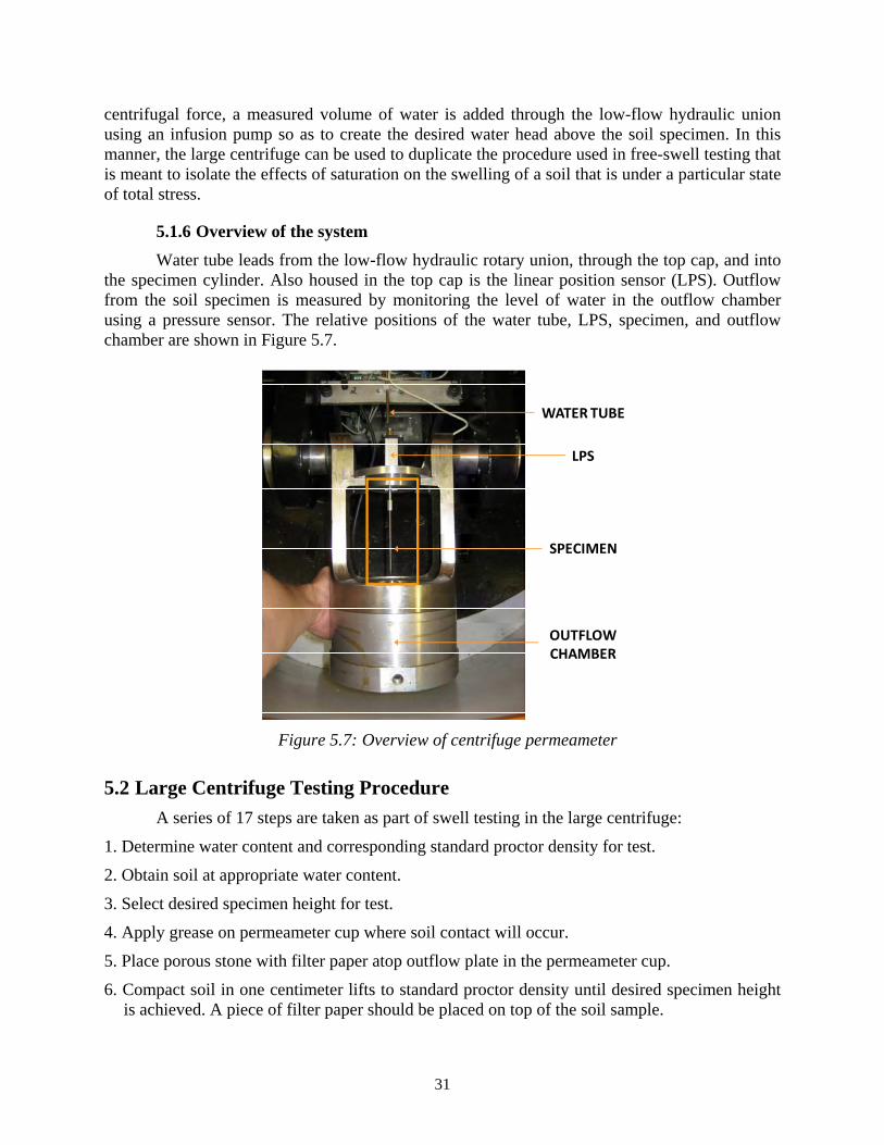
5.1.6 Overview of the system Water tube leads from the low-flow hydraulic rotary union, through the top cap, and into
the specimen cylinder. Also housed in the top cap is the linear position sensor (LPS). Outflow from the soil specimen is measured by monitoring the level of water in the outflow chamber using a pressure sensor. The relative positions of the water tube, LPS, specimen, and outflow chamber are shown in Figure 5.7.
Figure 5.7: Overview of centrifuge permeameter
5.2 Large Centrifuge Testing Procedure A series of 17 steps are taken as part of swell testing in the large centrifuge:
1. Determine water content and corresponding standard proctor density for test.
2. Obtain soil at appropriate water content.
3. Select desired specimen height for test.
4. Apply grease on permeameter cup where soil contact will occur.
5. Place porous stone with filter paper atop outflow plate in the permeameter cup.
6. Compact soil in one centimeter lifts to standard proctor density until desired specimen height is achieved. A piece of filter paper should be placed on top of the soil sample.
OUTFLOW CHAMBER
LPS
LOCATION OFSPECIMENCHAMBER
WATER TUBE

32
8. Place a porous stone on top of the sample to support the linear position senor arm.
9. Measure the distance from the top of the permeameter cup to the top of the upper porous plate with a Vernier caliper at four evenly spaced points around the permeameter cup.
10. Add water on top of soil sample to desired water height.
11. Fasten top cap with linear position sensor to top of permeameter cup.
12. Set centrifuge RPM to desired speed and start the data acquisition system to begin recording voltages from the LDT and the outflow transducer.
13. Run test until the soil specimen has reached a constant height and a steady state flow rate has been achieved.
14. Stop the test and weigh the specimens,
15. Suction off water from the top of the specimen and re-weigh.
16. Measure the distance from the top of the permeameter cup to the top of the upper porous plate with a Vernier caliper at four evenly spaced points around the permeameter cup.
17. Remove the soil specimens from the permeameter cylinders and determine their gravimetric water contents.
With the instrumentation and testing apparatus in place, this testing procedure is straight-
forward to follow in the laboratory. With initial training and limited oversight a laboratory technician could conduct the test and produce good testing results. Appendix A provides additional information regarding the testing procedures for the centrifuge permeameter.
5.3 Typical test results The large centrifuge has the advantage of being able to continually monitor the height of
the soil specimen. Prior to the addition of the linear position sensor, the height of the soil specimen was monitored by stopping the centrifuge and measuring the height with a Vernier caliper. The initial test was conducted on a 3 cm specimen of clay with 2 cm of overlying water at 50 G. The results from this test are shown in Figure 5.8. During the test, the specimen cylinder was also weighed and the flux rate from the specimen was calculated. The resulting flux rate versus time is shown in Figure 5.9. Based on the trends in strain and flux rate with time, the soil specimen reached its equilibrium strain under steady state flow after 3-4 days. It should be noted, however, that the scatter in the strain is considerable. Scatter from small centrifuge tests was originally found to be considerable but was later reduced as the testing procedure was refined. Since the addition of the linear position sensor, the height of the soil specimen can be continually monitored. The resulting trend in vertical strain with time is show for the test shown in Figure 5.10. These results are fairly typical for tests conducted in the large centrifuge.

33
Figure 5.8: Initial large centrifuge testing results
Figure 5.9: Outflow results from initial large centrifuge test
0
5
10
15
20
25
30
0 1 2 3 4 5 6 7
Stra
in (%
)
Elapsed time (days)
Sample 1
Sample 2
1.E-07
1.E-06
1.E-05
1.E-04
0 1 2 3 4 5 6 7
Flux
rate
(cm
/s)
Elapsed time (days)
Sample 1 - top
Sample 1 - base
Sample 2 -top
Sample 2 - base
34
Figure 5.10: Typical results from large centrifuge testing using the a linear position sensor
5.4 Key capabilities of the large centrifuge The large centrifuge has several key capabilities that set it apart from small centrifuge
testing. Specifically, the solid-state data acquisition system capable of sustaining high G levels gives the ability for in-flight data acquisition. Currently, this system is being used to measure specimen heights and outflow rates from soil specimens. In the small centrifuge, the height and outflow rates can be attained only by stopping the tests to take measurements. Additionally, properties that have been previously monitored using the large centrifuge and have the potential to be used in the future for highly plastic clay include suction and water content monitoring. The large centrifuge also has the advantage of being equipped with a low-flow hydraulic rotary union. This gives the experimenter the ability to control the water level during testing and to add water once the specimen is already in flight to ensure that the soil is under the correct total stress state before swelling is monitored.
0 0.5 1 1.5 2Time (days)
0
2.5
5
7.5
10
Ver
tical
stra
in (%
)

35
Chapter 6. Parametric Evaluation
A series of centrifuge tests were performed to understand the effect that the various variables had on test results. The four variables evaluated in this study include specimen height, water head, overburden pressure, and g-level. The baseline was a two centimeter specimen, with two centimeters of water head, minimum overburden spun at 200 g’s. Each parameter was varied individually and is discussed in detail in the following sections.
6.1 Specimen Height Specimen heights were varied from one centimeter up to four centimeters. Figure 6.1
shows strain versus time for three samples at different specimen heights. The following trends were noticed and were used to decide the standard specimen height:
• With increasing specimen height, the final strain is reduced. This is a result of an increase in effective stress in the sample.
• With increasing specimen height, testing time is increased.
• The measurement techniques used in both the small and large centrifuge systems have an accuracy of approximately 0.02 centimeters. With increasing specimen height the magnitude of this error in the measured strain is reduced.
A standard specimen height of one centimeter was chosen. The two main factors that
resulted in this choice were the longer test times from larger samples and the fact that 1g free-swell tests are performed on samples of similar size. The increased effect of measurement error was not considered to be enough to prevent the use of a one centimeter sample height.
Figure 6.1: Effect of sample heights on measured swell (200G with 2cm water head)
0%
2%
4%
6%
8%
10%
12%
14%
16%
18%
20%
0 50 100 150 200 250 300
Time (hrs)
Stra
in (%
)
2cm
3cm
4cm
36
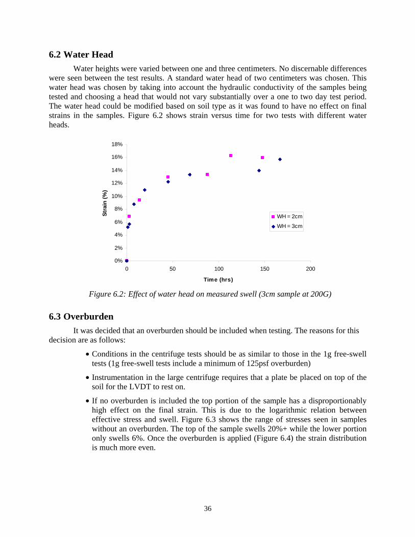
6.2 Water Head Water heights were varied between one and three centimeters. No discernable differences
were seen between the test results. A standard water head of two centimeters was chosen. This water head was chosen by taking into account the hydraulic conductivity of the samples being tested and choosing a head that would not vary substantially over a one to two day test period. The water head could be modified based on soil type as it was found to have no effect on final strains in the samples. Figure 6.2 shows strain versus time for two tests with different water heads.
Figure 6.2: Effect of water head on measured swell (3cm sample at 200G)
6.3 Overburden It was decided that an overburden should be included when testing. The reasons for this
decision are as follows:
• Conditions in the centrifuge tests should be as similar to those in the 1g free-swell tests (1g free-swell tests include a minimum of 125psf overburden)
• Instrumentation in the large centrifuge requires that a plate be placed on top of the soil for the LVDT to rest on.
• If no overburden is included the top portion of the sample has a disproportionably high effect on the final strain. This is due to the logarithmic relation between effective stress and swell. Figure 6.3 shows the range of stresses seen in samples without an overburden. The top of the sample swells 20%+ while the lower portion only swells 6%. Once the overburden is applied (Figure 6.4) the strain distribution is much more even.
0%
2%
4%
6%
8%
10%
12%
14%
16%
18%
0 50 100 150 200
Time (hrs)
Stra
in (%
)
WH = 2cm
WH = 3cm

37
Figure 6.3: Stress Ranges Without Overburden
Figure 6.4: Stress Ranges With Overburden
0
2
4
6
8
10
12
14
16
18
20
0 500 1000 1500 2000
Effective Stress (psf)
Swel
l (%
)
0
2
4
6
8
10
12
14
16
18
20
0 500 1000 1500 2000
Effective Stress (psf)
Swel
l (%
)
Range of stresses seen in sample
Range of stresses seen in sample
Overburden
38
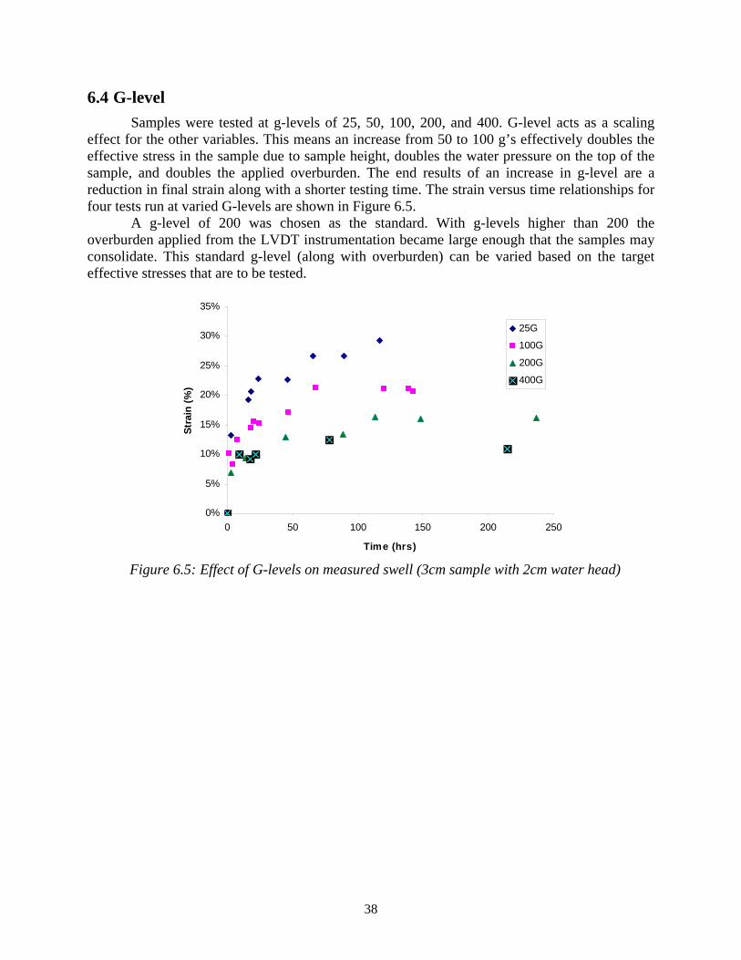
6.4 G-level Samples were tested at g-levels of 25, 50, 100, 200, and 400. G-level acts as a scaling
effect for the other variables. This means an increase from 50 to 100 g’s effectively doubles the effective stress in the sample due to sample height, doubles the water pressure on the top of the sample, and doubles the applied overburden. The end results of an increase in g-level are a reduction in final strain along with a shorter testing time. The strain versus time relationships for four tests run at varied G-levels are shown in Figure 6.5.
A g-level of 200 was chosen as the standard. With g-levels higher than 200 the overburden applied from the LVDT instrumentation became large enough that the samples may consolidate. This standard g-level (along with overburden) can be varied based on the target effective stresses that are to be tested.
Figure 6.5: Effect of G-levels on measured swell (3cm sample with 2cm water head)
0%
5%
10%
15%
20%
25%
30%
35%
0 50 100 150 200 250
Time (hrs)
Stra
in (%
)
25G
100G
200G
400G
39
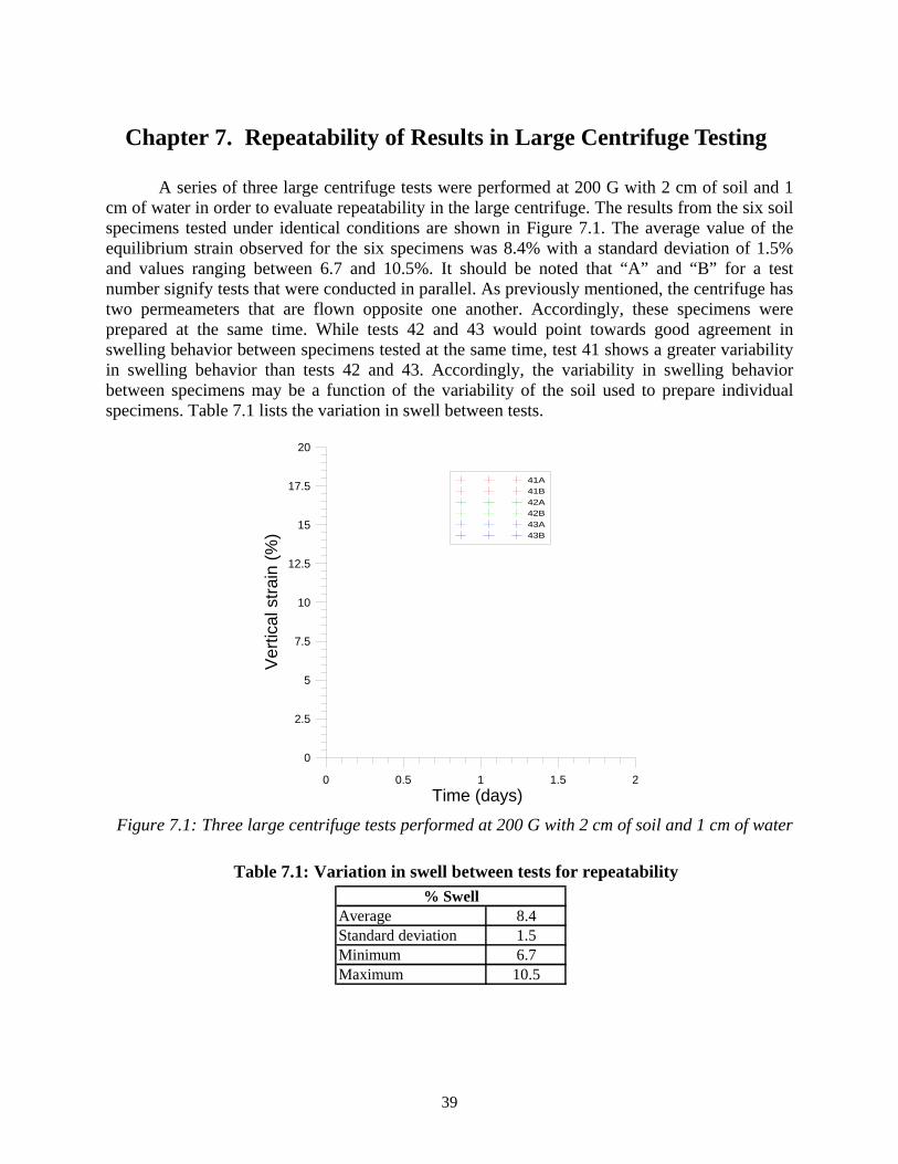
Chapter 7. Repeatability of Results in Large Centrifuge Testing
A series of three large centrifuge tests were performed at 200 G with 2 cm of soil and 1 cm of water in order to evaluate repeatability in the large centrifuge. The results from the six soil specimens tested under identical conditions are shown in Figure 7.1. The average value of the equilibrium strain observed for the six specimens was 8.4% with a standard deviation of 1.5% and values ranging between 6.7 and 10.5%. It should be noted that “A” and “B” for a test number signify tests that were conducted in parallel. As previously mentioned, the centrifuge has two permeameters that are flown opposite one another. Accordingly, these specimens were prepared at the same time. While tests 42 and 43 would point towards good agreement in swelling behavior between specimens tested at the same time, test 41 shows a greater variability in swelling behavior than tests 42 and 43. Accordingly, the variability in swelling behavior between specimens may be a function of the variability of the soil used to prepare individual specimens. Table 7.1 lists the variation in swell between tests.
Figure 7.1: Three large centrifuge tests performed at 200 G with 2 cm of soil and 1 cm of water
Table 7.1: Variation in swell between tests for repeatability
0 0.5 1 1.5 2Time (days)
0
2.5
5
7.5
10
12.5
15
17.5
20
Ver
tical
stra
in (%
)
41A41B42A42B43A43B
Average 8.4Standard deviation 1.5Minimum 6.7Maximum 10.5
% Swell

40

41
Chapter 8. Comparison of Small and Large Centrifuge Test Results
Three tests were conducted in the small centrifuge in order to compare tests results from large and small centrifuge testing. This corresponds to a series of six specimens. The same parameters used to evaluate repeatability in the large centrifuge (i.e., 200 G, 2 cm of soil, and 1 cm of water) were used for the small centrifuge tests. The results from the small centrifuge testing are plotted with the results from large centrifuge testing in Figure 8.1. Composite curves for the small and large centrifuge test results were determined by the vertical strain for each test at each instant in time. The resulting curves represent the average swelling behavior of the soil and are shown in Figure 8.2. A comparison of the composite curve demonstrates very good agreement between the swelling behavior observed in the large and small centrifuges. The equilibrium strains are compared in terms of average, standard deviation, and minimum and maximum values in Table 8.1. The average equilibrium strain for large and small centrifuge testing is within 0.1 % of each other. The standard deviation for large and small centrifuge testing is also within 0.1% of each other. The good agreement between tests conducted in the large centrifuge and small centrifuge demonstrates the validity of validity of centrifuge swell testing in that similar results were found in separate testing environments.
Figure 8.1: Comparison of small and large centrifuge results

42
Figure 8.2: Composite curve for small and large centrifuge tests
Table 8.1: Comparison of small and large centrifuge test results
% Swell Small LargeAverage 8.3 8.4Standard deviation 1.4 1.5Minimum 6.5 6.7Maximum 9.9 10.5

43
Chapter 9. Comparison between 1G and nG Tests
As shown by results from 1g free-swell testing, the relationship between swell and effective stress is semi-logarithmic. This poses a problem when attempting to directly compare 1g and Ng tests because of the comparatively larger range of stress experienced by samples in the centrifuges.
Stresses in free-swell tests vary less than 5 psf across the sample. Considering the overburdens applied to the free-swell tests, the 5 psf differences are negligible and the stress can be considered constant across the sample. This is not the case for the Ng tests where effective stress can vary up to 1000 psf across the sample. Because of the difference in the state of stress in the samples, comparison between 1g and Ng tests must be done indirectly by comparing effective stress vs. swell relationships.
Comparison was initially made by using the known effective stress vs. swell relation determined from the 1g free-swell tests. This relation was then used to calculate the total swell that would be expected given the range of stresses seen in a centrifuge test. If the calculated swell using the 1g relation matched with test results from the respective Ng tests, both the Ng and 1g tests would be based on the same fundamental effective stress vs. strain relation and the relation between 1G and NG tests would be validated.
In order to complete this comparison the range of stresses in the centrifuge must be calculated. The next section is devoted to the analysis of effective stresses seen in a sample tested under increased G-levels.
9.1 Determining Effective Stress in the Centrifuge Calculating total stresses in a centrifuge sample is fairly straightforward. Overburden of a
layer can be calculated by multiplying the unit weight of the layer by its thickness times the average g-level for the layer. Because G-level varies with radius the average g-level over the layer must be used. The average can be calculated by integrating the g-level across the layer (with respect to radius) and dividing by the layer thickness. However, as g-level varies linearly with radius, the average can be taken simply as the g-level calculated at mid-height of each layer.
Using the above method total stress can be calculated at any point in a centrifuge test sample. In order to determine the effective stress the pore pressures must be known and subtracted from the total stress.
9.1.1 Accounting for Varied G-level
Using the assumption that total head decreases linearly throughout the sample (Darcian flow, constant hydraulic conductivity and area) and is zero at the base of the specimen, total head can be expressed as:
)1()( )(
)(ab
arrrr
at hrh −−+=
(9.1) where: r is the radius where the head is desired;
ah is the known head at the top of the sample;
ar is the radius at the top of the sample;

44
br is the radius at the base of the sample (datum).
Elevation head can be calculated as the distance above the datum multiplied by the average g-level across that distance:
∫−
== br
r
be
rrdrrrh
2)(
)(222
2 ωω (9.2)
Given that pet hhh += , the pressure head at any radius can be calculated using:
2)(
)1()(2222
)()( ωrr
hrh brrrr
ap ab
a−
−+= −− (9.3)
where: r is the radius where the head is desired;
ah is the known head at the top of the sample;
ar is the radius at the top of the sample;
br is the radius at the base of the sample (datum); ω is the rotational velocity (constant).
The effect of the g-level varying across the sample is minimal when compared to the
assumption of a constant g-level. Figure 9.1 shows the slightly lower pore pressures across a 4 cm sample with 2 cm of water head when a varying g-level is taken into account.
Figure 9.1: Pore water pressures assuming constant and varied g-level
9.1.2 Effect of Varying Hydraulic Conductivity Many factors may affect the hydraulic conductivity of soil across a sample in a centrifuge
test. Several are listed here:
0
0.5
1
1.5
2
2.5
3
3.5
4
4.5
0 50 100 150 200 250 300
Pressure head (cm)
Dis
tanc
e (c
m)
Linearly increasing g-level
Constant g-level throughout sample
45
• Particle migration causing fines to move with flow towards the base of the specimen resulting in a lower hydraulic conductivity in the lower portion of the sample.
• Higher stress levels in lower portions of the sample resulting in lower void ratio and lower hydraulic conductivity
• Clogging of filter paper from particle migration and base of specimen resulting in lower hydraulic conductivity at the base of the specimen.
• More swelling in the upper portion of the sample due to lower stresses resulting in higher hydraulic conductivities in the top of specimens.
All of the factors result in hydraulic conductivity decreasing in a sample from top to
bottom. The effect of non-uniform hydraulic conductivity on the pore pressures across the sample can be analyzed by assuming a linear drop in hydraulic conductivity across the sample such that:
)()( baab
aa kk
rrrrkrk −
−−
+= (9.4)
where: r is the radius where the head is desired;
ar is the radius at the top of the sample;
br is the radius at the base of the sample (datum);
ak is the hydraulic conductivity at the top of the sample;
bk is the hydraulic conductivity at the base of the sample. Using this relation, a function for hydraulic gradient across the sample is defined as:
Arkqri)(
)( −= (9.5)
where: A is the cross-sectional area of the sample; q is the flow rate through the sample.
By integrating )(ri from br to r the resulting function is total head as follows:
)(|))(ln(|)(
)(|))(ln(|)(
)(ba
abbababa
ba
abbabbabat kkA
rkrkrkkrrqkkA
rkrkrkkrrqrh
−+−−−
−−
+−−−=
(9.6) As previously discussed, elevation head can be expressed as was shown in Equation 9.2:
2)(
)(222 ωrr
rh be
−= (9.2)
and therefore the resulting function for pressure head is:
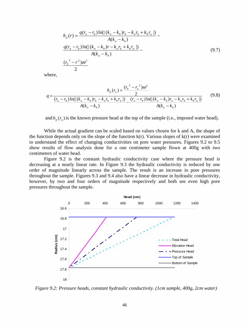
46
2)(
)(|))(ln(|)(
)(|))(ln(|)(
)(
222 ωrr
kkArkrkrkkrrq
kkArkrkrkkrrq
rh
b
ba
abbababa
ba
abbabbabap
−
−−
+−−−
−−
+−−−=
(9.7)
where,
)(|))(ln(|)(
)(|))(ln(|)(
2)(
)(222
ba
abbaababa
ba
abbabbaba
abap
kkArkrkrkkrr
kkArkrkrkkrr
rrrh
q
−+−−−
−−
+−−−
−+
=
ω
(9.8)
and )( ap rh is the known pressure head at the top of the sample (i.e., imposed water head).
While the actual gradient can be scaled based on values chosen for k and A, the shape of
the function depends only on the slope of the function k(r). Various slopes of k(r) were examined to understand the effect of changing conductivities on pore water pressures. Figures 9.2 to 9.5 show results of flow analysis done for a one centimeter sample flown at 400g with two centimeters of water head.
Figure 9.2 is the constant hydraulic conductivity case where the pressure head is decreasing at a nearly linear rate. In Figure 9.3 the hydraulic conductivity is reduced by one order of magnitude linearly across the sample. The result is an increase in pore pressures throughout the sample. Figures 9.3 and 9.4 also have a linear decrease in hydraulic conductivity, however, by two and four orders of magnitude respectively and both see even high pore pressures throughout the sample.
Figure 9.2: Pressure heads, constant hydraulic conductivity. (1cm sample, 400g, 2cm water)
16.6
16.8
17
17.2
17.4
17.6
17.8
18
0 200 400 600 800 1000 1200 1400
Head (cm)
Rad
ius
(cm
)
Total Head
Elevation Head
Pressure Head
Top of Sample
Bottom of Sample

47
Figure 9.3: Pressure heads, one order of magnitude change in hydraulic conductivity. (1cm
sample, 400g, 2cm water)
Figure 9.4: Pressure heads, two orders of magnitude change in hydraulic conductivity. (1cm
sample, 400g, 2cm water)
16.6
16.8
17
17.2
17.4
17.6
17.8
18
0 200 400 600 800 1000 1200 1400
Head (cm)
Rad
ius
(cm
)
Total Head
Elevation Head
Pressure Head
Top of Sample
Bottom of Sample
16.6
16.8
17
17.2
17.4
17.6
17.8
18
0 200 400 600 800 1000 1200 1400
Head (cm)
Rad
ius
(cm
)
Total Head
Elevation Head
Pressure Head
Top of Sample
Bottom of Sample

48
Figure 9.5: Pressure heads, four orders of magnitude change in hydraulic conductivity. (1cm
sample, 400g, 2cm water)
The most apparent effect of a sample with decreasing hydraulic conductivity is the increase in pore water pressure in the sample. This causes a lower effective stress in the sample and must be taken into account when comparing 1g vs. Ng tests. Several simplified pore water pressure distributions were selected, as discussed next.
9.1.3 Selection of Pore Water Pressure Profiles For analysis of 1g vs. Ng tests three pore water pressure distributions were chosen to
represent the range of pressures that might be obtained in a sample due to the uncertainty of hydraulic conductivities. They are as follows:
1. A linearly decreasing pore water pressure to represent a free flowing condition.
2. A constant power water pressure distribution to represent a case with decreasing hydraulic conductivity across the sample.
3. A linearly increasing pore water pressure distribution to represent a significant decrease in hydraulic conductivity across the sample. Pore pressures representing a no-flow case were used.
These will be referred to PWP1, PWP2, and PWP3 respectively. They are shown in
Figure 9.6 on a one centimeter sample at 400g with two centimeters of water head.
16.6
16.8
17
17.2
17.4
17.6
17.8
18
0 200 400 600 800 1000 1200 1400
Head (cm)
Rad
ius
(cm
)
Total Head
Elevation Head
Pressure Head
Top of Sample
Bottom of Sample

49
Figure 9.6: Simplified Pore Water Pressure Distributions
9.2 Validation of Ng Results from 1g Relation In order to compare Ng tests with 1g tests the logarithmic relationship of strain versus
effective stress (from 1g tests) was used. This relation was used to predict the magnitude of strain values that should be expected from an Ng test, given the ranges in effective stresses seen in the Ng tests. If this predicted strain is similar to the measured strain from the Ng test, a relation between the Ng and 1g tests would be confirmed.
In order to predict strain for the Ng tests the following steps were taken:
• The sample height was discretized into .1 cm increments.
• Average effective stress was calculated for each increment.
• Strain vs. effective stress relation (from 1g tests) was used to calculate swell for each layer
• Effective stresses were recalculated using new unit weights (corrected for swell) and layer heights.
• Strain was recalculated. The process was repeated until strain varied less than .05% between iterations.
This process was completed using the three of the simplified pore water pressure
distributions and for three different Ng test sets. The resulting calculated swells for each of the simplified pore water pressure distributions are shown in Figure 9.7 versus the measured swell for the test set. The three of the distributions predict swells that are lower than those measured in the centrifuge. PWP3 gives results closest to that measured in the centrifuge.

50
Figure 9.7: Calculated Swell vs. Measured (varied PWPs)
The under-prediction of swell in the calculations based on 1g tests could be attributed to an over-prediction of effective stress in the samples. However, because PWP3 represents the maximum pore water pressures that could logically be seen in the sample, it was decided that an over-prediction of effective stresses was unlikely. One reason for this variance in swell could be the difference in measurement procedure between the 1g swell tests and the Ng centrifuge tests.
The free-swell tests used LVDTs placed on top of a porous stone to measure swell. If the sample is not in perfect contact with the porous stone, any initial swell of the sample would be ignored until perfect contact is achieved. The Ng tests used a different method that involved suctioning water off and measuring the volume of suctioned water (discussed in section 4.3). This method does not require perfect contact and would measure the initial swell resulting in larger measured strains.
Several simplified experiments were run to determine the magnitude of this effect. It was concluded that the LVDTs would on average ignore 1.5mm (1.5% swell for the 1cm samples used) of swell given our compaction techniques. The measured swells from Ng tests were reduced by 1.5% and have been graphed as “Corrected Ng” in Figure 9.8.
0
1
2
3
4
5
6
7
8
9
Test 1 Test 2 Test 3
Swel
l (%
) PWP 1
PWP 2
PWP 3
Measured Ng

51
Figure 9.8: Calculated Swell vs. Measured (corrected)
Once the correction has been applied the calculated swells using PWP3 match well with the Ng tests. This provides an indirect comparison of the 1g and Ng tests. For the three test sets considered all fall within 1.5% with an average error of 0.6%. The testing setups are shown in Table 9.1 along with the calculated and measured strains. The measured swell from each test set is the average for all tests run with that specific setup.
Table 9.1: Test Set Data G-
Level
Water Height (cm)
Sample Height (cm)
Overburden (g)
Strain (%)
Calculated Corrected
Ng Test Set 1 400 2 1 15 6.6 6.4
Test Set 2 200 2 1 53 5.5 6.7
Test Set 3 200 2 1 78 3.9 3.5
It would be beneficial to validate some of the assumptions that are used in this
comparison. Particularly, it would be useful to:
• Determine if clogging that would result in pore water pressures close to that of PWP3 (used in analysis) occurs in the Ng tests.
• Pursue further testing into the effect the measurement system has on the reported swell.
0
1
2
3
4
5
6
7
8
9
Test 1 Test 2 Test 3
Swel
l (%
) PWP 3
Corrected Ng
Measured Ng

52
9.3 Determining Stress-Strain Relation from Ng Tests While the Ng tests have been confirmed to correlate well with 1g tests, a method is still
required obtain the relationship between swelling and effective stress from Ng tests. The method used for determining the stress-strain relation is as follows:
• Perform three or more Ng tests at varying effective stress levels.
• Assume an effective stress vs. swell relationship such that, Swell (%) = A*ln(Effective Stress) + B.
• Calculate the swell for each of the test sets using the method discussed in section 9.2 using the assumed effective stress vs. swell relation. Consider pore water pressure distribution three (PWP3) in the calculations, as it was found to be the most accurate (section 9.2).
• Determine the coefficients A and B that result in the least error between measured swell and predicted swell for all test sets using the least squares method.
This process was completed for the three previously discussed test sets listed in Table
9.1. The Solver application in Microsoft Excel was used to find values of A and B which resulted in the least error of predicted vs. measured swell. The resulting coefficients were -5.517 and 44.15 for A and B respectively. These compare well with the coefficients found from the free-swell tests (-5.16 and 40.99 respectively). Figure 9.9 illustrates the effective stress vs. swell relationship found from the 1g free-swell tests (black) along with the relationship found using the three Ng test sets (red). The three test sets that populated the Ng best fit are also plotted over their respective effective stresses and the scatter from the best fit is shown.
Figure 9.9: 1g best fit vs. Ng best fit.
0
2
4
6
8
10
12
14
16
18
20
0 500 1000 1500 2000
Effective Stress (psf)
Swel
l (%
)
Ng Best Fit
Free Sw ell (1g) Best Fit
Test Set 1
Test Set 2
Test Set 3

53
The swell values calculated using the nG best fit relation are shown in Figure 9.10 as a function of the results measured from the Ng tests. The variance is low with the second test set being worst at 1.2% lower than the measured swell.
Figure 9.10: Ng predicted vs. measured.
This method was found to provide good resulting, and is suitable for predicting the effective stress vs. swell relationship using the three test sets. However, several things are worth noting:
• The final relation (coefficients A and B) is very sensitive to small changes in swell of the test sets.
• The final relation is accurate only for effective stress ranges seen in the test sets. It would be best to populate the best fit with tests over a wide range of effective stresses. For example, one centimeter samples could be flown at 100, 200, and 400 g’s in order to have data from effective stresses ranging from approximately 50 to 1500 psf.
• A single sample could be flown at progressively higher g-levels (100, 200, 400 for example) to get the multiple data points needed to populate the best fit curve. This would allow a three day test (1 day for each g-level) to produce an effective stress vs. swell relation accurate over a wide range of stresses.
0.00
1.00
2.00
3.00
4.00
5.00
6.00
7.00
8.00
1 2 3
Test Set
Swel
l (%
)
Predicted Sw ell
Measured Sw ell (corrected)

54
55
Chapter 10. Conclusions
The research team successfully used centrifuge technology to evaluate the swelling properties of highly plastic clay. Testing performed for this project demonstrated the feasibility of expeditiously measuring the swelling potential of highly plastic clays using a centrifuge permeameter. Specifically, a time period of 24 hours was found necessary for a 1 cm specimen of compacted clay to swell to an equilibrium height in the centrifuge permeameter. This is in contrast to the one month of time required for free-swell test specimens to reach equilibrium. Good agreement was found between tests conducted in the large centrifuge and small centrifuge. Specifically, the average equilibrium strain for large and small centrifuge testing was within 0.1% of one another. Finally, a methodology for determining the stress-strain relationship from centrifuge testing was presented and validated. The relationship can be developed by running three 24 hour tests on a single specimen, yielding a total testing time of 3 days.
Centrifuge permeameter technology has great potential to provide engineers with a means of quickly and directly attaining the swelling of highly plastic clay. Rather than having to resort to index properties to predict soil swelling, centrifuge permeation of highly plastic clays allows for the direct, expeditious, and consistent experimental measurement of swelling.
Continued centrifuge testing would be instrumental in order to allow characterization of expansive clays that are typically encountered in TxDOT pavement projects. Specifically, an additional testing program using high plasticity soils from specific sites in the state would allow quantification of the potential heave at these sites. Ultimately, the characterization of expansive clays at specific sites would allow comparison of experimentally predicted vertical raise values with those obtained using less rigorous approaches such as the PVR based on index clay properties.

56

57
References
Allen , J., 2004, “Forced Ventilated Swell-Shrink Test for Potential Vertical Expansive Soil Movement.” Thesis, Master of Science in Engineering, The University of Texas at Austin.
American Society of Testing and Materials, 2000, “Standard Test Method for Determining Unsaturated and Saturated Hydraulic Conductivity in Porous Media by Stead-State Centrifugation.” ASTM D6527-00. West Conshohocken, Pennsylvania.
Bear, J., Dynamics of Fluids in Porous Media. Elsevier, New York, 1943.
Cinicoioglu, O., Znidarcic, D., and Ko, H, 2006. “A New Centrifugal Testing Method: Descending Gravity Test.” Geotechnical Testing Journal, Vol. 29, No. 5, pp. 1-10.
Covar, A. P., and Lytton, R. L., 2001, “Estimating soil swelling behavior using soil classification properties.” Expansive Clay Soils and Vegetative Influences on Shallow Foundations, ASCE Geotechnical Publication No. 115, American Society of Civil Engineers, Reston, VA, pp. 44–63.
Jones , D.E., and Holtz, W.G., 1973, “Expansive Soils – The Hidden Disaster,” Civil Engineering, Vol. 43, no. 8, pp. 49-51.
Kuhn, J., 2005, “Effect of Cracking on the Hydraulic Properties of Unsaturated Highly Plastic Clays.” MS thesis, The University of Texas, Texas.
Lee, J., and Fox, P. , 2005, “Efficiency of Seepage Consolidation for Preparation of Clay Substrate for Centrifuge testing.” Geotechnical Testing Journal, Vol. 28, No. 6, pp.1-9.
Lu, N., and Likos, W.J, 2005, Unsaturated Soil Mechanics, Wiley, New York.
Lytton, R.L., Aubeny, C., and Bulut, R., May 2006, “Design Procedure for Pavements on Expansive Soils: Volume 2,” Texas Transportation Institute, Report # 0-4518-1 (V2).
Lytton, R.L., Aubeny, C., and Bulut, R., August 2005, “Design Procedure for Pavements on Expansive Soils: Volume 1,” Texas Transportation Institute, Report # 0-4518-1 (V1).
Lytton, R.L., Aubeny, C., and Bulut, R., June 2005, “Design Procedure for Pavements on Expansive Soils: Volume 3,” Texas Transportation Institute, Report # 0-4518-1 (V3).
Lytton, R.L., Aubeny, C., and Bulut, R., July 2005, “Re-evaluation of Potential Vertical Rise Design Procedures 0-4518-S,” Texas Transportation Institute, Report # 0-4518-S.
McCartney, J., 2006, “Measurement of the Hydraulic Characteristics of Unsaturated Soils using a Centrifuge Permeameter,” Comprehensive Proposal, The University of Texas at Austin.
McCartney, J.S., and Zornberg, J.G. (2005). “The Centrifuge Permeameter for Unsaturated Soils (CPUS).” Proceedings of the International Symposium on Advanced Experimental

58
Unsaturated Soil Mechanics, Experus 2005, Trento, Italy, June 27-29, A.A. Balkema, pp.299-304.
McDowell, C., 1956, “Interrelationships of loads, volume change, and layer thickness of soils to the behavior of engineering structures.” Highway Research Board, Proc. 35th Annual Meetings, Pub. No. 426, Washington, DC, pp. 754-772.
Olson, Roy E. 2007 Course Notes on Incremental Vertical-Flow Consolidation Test, Consolidation and Settlement of Soft Soils.
Mitchell, R.J., 1994, “Centrifuge techniques for testing clay liner samples.” Canadian Geotechnical Journal, No. 31, pp. 577-583.
Puppala, A., and Hoyos, L., Ongoing, “Realistic design guidelines for low classification roads in high PI clays.” Texas Department of Transportation Project #0-5430.
Robinson, R.G., Tan, T.S., and Lee, F.H., 2003, “A Comparative Study of Suction-Induced Seepage Consolidation Versus Centrifuge Consolidation.” Journal of Geotechnical Testing, March 2003, Vol. 26, No.1., pp 1-10.
Singh, D., and Gupta, A., 2000, “Modeling hydraulic conductivity in a small centrifuge.” Canadian Geotechnical Journal, No. 37, pp. 1150-1155.
Terzaghi, K., 1943, Theoretical Soil Mechanics. John Wiley and Sons, New York.
Weisberg, E, and Frydman, S., 1990, “Study of Flow in Compacted Columns of Swelling Clay.”
Zornberg, J.G. and Kuhn, J., 2007, Field Suction and Effect of Cracking in Highly Plastic Clay, Center for Transportation Research, Report # 0-5202-1 through # 0-5202-3.

59
Appendix A: Small Centrifuge Testing Procedure
A1. Soil Preparation 1. Soil should be mixed to optimum water content and allowed to equilibrate for 48 hours after
mixing. This ensures an even moisture distribution throughout the soil mix. Record the target dry unit weight ( , ) and target water content ( , ). A soil sample should always be taken directly prior to testing and measured for water content.
Note: During testing, a zone of , +/- 0.5% was used as acceptable.
A2. Centrifuge Cup Preparation and Soil Compaction 2. Insert the porous supporting plate into the permeameter cup and place a filter paper on top of
the plate. Lubricate the inside of the cup approximately 2 cm up from the porous plate.
3. Weigh the mass of the centrifuge cup (including the detachable outflow chamber), supporting plate, and two filter papers. One filter paper should already have been inserted on top of the supporting plate. The second will be placed on top of the compacted soil but should be included in this measurement. Record the mass ( ). Remove the detachable outflow chamber and weigh ( ). Reattach after weighing.
4. Insert appropriate mass of soil at optimum moisture into centrifuge cup. This required mass should be calculated as , 1 , . The soil should then be compacted to one centimeter height using kneading compaction. Proper compaction is important and care should be taken to obtain a sample height as close to one centimeter as possible.
5. Place the second filter on top of the compacted soil and weight the mass of the cup ( . This mass should be checked to ensure proper soil compaction and mass ( = + .
Note: During testing +/- 1g was acceptable.
A3. Determining Initial Sample Height 6. Water should be gently poured on top of the specimen to a height of approximately 2 cm. Air
bubbles should be removed including those stuck underneath the filter paper. The mass of the cup with water on top should be recorded ( ). Using a caliper, the distance from the base of the compacted soil to base of the water meniscus should be measured ( , ).
Note: It is useful to either mark a line or machine a groove in the centrifuge cup at the location of the base of the soil. This reduces variance in measurements as the caliper can be placed on the line or in the groove and measured from the same precise location.
7. One half to one centimeter of water should then be suctioned off. The mass of the cup ( ) and distance from the base of the compacted soil to the base of the meniscus ( , ) should again be measured.

60
8. A porous supporting disk should then be placed on top of the soil sample. The effective height of the porous disk should be calculated and recorded . The porous disk is used to distribute the overburden across the soil sample.
Note: The effective height of the porous disk refers to the increase in height of water due to the submerged porous disk. This should be calculated experimentally by determining ∆L (change in distance from base of soil to base of water meniscus) when the porous disk is submerged.
9. (optional *) Water should be added to a height of approximately 2 cm. The mass of the cup with water on top should be recorded ( ). Once again air bubbles must be removed especially in the pores of the disk. Using a caliper, the distance from the base of the compacted soil to base of the water meniscus should be measured ( , ).
10. (optional *) One half to one centimeter of water should then be suctioned off. The mass of the cup ( ) and distance from the base of the compacted soil to the base of the meniscus ( , ) should again be measured.
11. (optional *) The remainder of the water should be suctioned off around the upper porous disk. Record the mass of the cup ( .
A4. Applying Water Head and Overburden 12. A mass of water should be poured onto the sample equaling a head of 2 cm. This can be
calculated as 2 . The mass of the cup should then be recorded ( .
13. Insert weights equaling the desired overburden mass on top of the porous disk. The cup should be inserted into the centrifuge cup holder and the rubber stopper placed in the opening of the centrifuge cup to prevent excessive evaporation.
A5. Spinning the Centrifuge 14. The centrifuge should be started at the RPM desired for the particular test. Record the current
time ( ). The centrifuge should be allowed to spin for approximately 24 hours. Turn off the centrifuge, recording the time ( ). Wait until the centrifuge has come to a complete stop and remove the cup from the centrifuge holder and the rubber stopper from the top. Remove the weights from the upper porous disk.
A6. Determining 24 Hour Sample Height (optional) 15. (optional **) Record the mass of the cup ( ) and distance from the base of the compacted
soil to the base of the meniscus ( , ).
16. (optional **) One half to one centimeter of water should then be suctioned off. The mass of the cup ( ) and distance from the base of the compacted soil to the base of the meniscus ( , ) should again be measured.

61
17. (optional **) The remainder of the water should be suctioned off around the upper porous disk. Record the mass of the cup ( . Remove the detachable outflow chamber and weigh ( ). Reattach after weighing.
A7. Re-applying Water Head and Overburden 18. A mass of water should be poured onto the sample equaling a head of two centimeters. This
can be calculated as 2 . The mass of the cup should then be recorded ( . Insert weights equaling the desired overburden mass on top of the porous disk.
A8. Spinning the Centrifuge 19. The cup should be inserted into the centrifuge cup holder and the rubber stopper placed in the
opening of the centrifuge cup to prevent excessive evaporation. The centrifuge should be started at the RPM desired for the particular test. Record the current time ( ).
20. The centrifuge should be allowed to spin for approximately 24 hours. Turn off the centrifuge recording the time ( ). Wait until the centrifuge has come to a complete stop and remove the cup from the centrifuge holder and the rubber stopper from the top. Remove the weights from the upper porous disk.
A9. Determining Final Sample Height 21. Record the mass of the cup ( ) and distance from the base of the compacted soil to the
base of the meniscus ( , ).
22. One half to one centimeter of water should then be suctioned off. The mass of the cup ( ) and distance from the base of the compacted soil to the base of the meniscus ( , ) should again be measured.
23. The remainder of the water should be suctioned off around the upper porous disk. Record the mass of the cup ( .
24. Remove the upper porous disk and pour approximately 2 cm of water in the cup. Record the mass of the cup ( ) and distance from the base of the compacted soil to the base of the meniscus ( , ).
25. One half to one centimeter of water should then be suctioned off. The mass of the cup ( ) and distance from the base of the compacted soil to the base of the meniscus ( , ) should again be measured.
26. The remainder of the water should be suctioned off. Record the mass of the cup ( . Remove the detachable outflow chamber and weigh ( ). Reattach after weighing.
62
27. The sample should then be removed from the centrifuge cup and oven dried to determine the final water content.
A10. Calculations
Initial Height: , , , , or , ,
Where:
, , ,
, , ,
, , , (optional)
, , , (optional)
is the effective height of the porous supporting disk.
24-hour Height: , ,2
Where:
, , ,
, , ,
is the effective height of the porous supporting disk.
Final Height: , , , ,4
Where:
, , ,
, , ,
63
, , ,
, , ,
is the effective height of porous supporting disk. Note: If , and , consistently vary from , and , the effective height may have been calculated incorrectly.
Final Strain:
Optional *: Additional initial sample height readings may be taken after the porous disk has been inserted. This allows for greater accuracy in the initial reading and the opportunity to ensure that the effective height of the porous disk, , being used is correct. This step requires additional time and allows the sample to swell under 1g conditionals; however, the researchers found if measurements are taken quickly the effect is minimal.
Optional **: A 24-hour reading may be taken. If new soils are being tested, incremental readings such as a 24-hour reading may be helpful to ensure that swelling has completed. If a soil type is being tested for the first time, it is recommended to take the 24-hour reading, perform a repeat of the 24-hour reading at 48 hours, and then perform the final height measurements at 72 hours.

64
65
Appendix B: Large Centrifuge Testing Procedure
The following steps outline the testing procedure for the large centrifuge permeameter. A
data sheet should be used for each test so that the technician performing the test records all of the necessary data.
B1. Preparation of Soil Specimen The soil specimen used for testing should be prepared in a similar manner to which soil in
the field is prepared during construction. If construction is to take place on a natural soil, then testing should be carried out on samples that are trimmed into the testing device. Testing for this study has been performed only on remolded samples and thus only the testing of remolded soils will be addressed. Preparation of the soil for a test on remolded soil is to proceed as follows:
a. Specific gravity test Perform a specific gravity measurement on the fraction of soil passing
the No. 4 sieve in accordance with ASTM D 854-02. b. Moisture content and density selection Determine the moisture density relationships for the
soil (ASTM D 698-00a; ASTM D 1557-02). Select a target moisture content and density for the test.
c. Soil processing Process an adequate amount of soil for running several tests. This processed
soil will be the source for your centrifuge test. Prior to testing, the soil was air-dried, crushed, and processed. After being air-dried and processed, the soil appeared tan in color. The soil was dried at a temperature of approximately 120°F, not exceeding 140°F according to ASTM D 698-00a so that changes in the soil properties would not occur.
d. Target moisture content Once the target water content and density are determined, sufficient
soil to form two specimens should be mixed to the target water content. The water content of the source soil should be determined and entered into the data sheet. Using the target water content and density, the mass of soil to be used from the source material and the mass of water that should be added should be determined. The phase diagrams in the data sheet should be filled out.
e. Moisture equilibration The mixed soil should be placed in an air-tight plastic bag for 48
hours. It is preferable that this plastic bag is kept in a humidity chamber for this 48-hour period.
B2. Preparation of Permeameter Cup For each test, the centrifuge cup must be properly cleaned, re-assembled, and weighed in
preparation for compacting the specimen into the permeameter cup.
a. Cleaning The permeameter cup should be cleaned with soap and water after each test. The permeameter cup should then be dried with a towel or left on an equipment rack to air-dry.
66
b. Grease application To minimize ring friction and sidewall leakage during testing, a thin layer of high vacuum grease should be spread around the inner wall of the permeameter cup. The easiest way to apply the grease is with the tip of one’s finger. In our laboratory we use Dow Corning High Vacuum Grease.
c. Ponding height The height to which water is to be ponded above the base plate should be
selected and the set-screws in the wall of the permeameter should be re-arranged as appropriate.
d. Permeameter weight The permeameter cylinder, base plate, top plate, filter papers, and
vacuum grease should be weighed together on a laboratory scale. e. Base plate and base filter paper The base plate is then placed inside of the permeameter
cylinder and a piece of filter paper is placed atop the porous plate. The filter papers that are used for the large centrifuge permeameter are pre-cut and are a product of Humboldt Manufacturing Company out of Schiller Park, Illinois. The filter paper is 2.8 inches (70 mm) in diameter and is model HM-4189.28.
f. Height determination In order that the initial and final heights of the soil specimen can be
determined, the distance from the top of the cup to the top of the base plate should be measured and noted as D_base in the data sheet.
B3. Soil Specimen Preparation The soil specimen is compacted in 1 cm lift up to the desired specimen height using a
March-Bellofram actuator air piston (product number 980-077-000). The air piston was outfitted with a 5-inch long, 0.5-inch diameter rod that we screwed onto the actuator air piston to serve as a compaction ram and used to impart energy into the soil. Prior to additional lifts, the surface of the soil is scarified.
1. Compaction height check Prior to starting compaction, a digital Vernier caliper is zeroed out
with the measurement from the top of the cup to the top of the base plate. The Vernier caliper is then raised 10 mm and locked in place. During the compaction procedure, this Vernier Caliper is intermittently used to measure the lift thickness.
2. Soil placement To start compaction, soil is placed in the cup and kneaded into place with
one’s finger. If this kneading is not carried out, the compaction foot will penetrate the soil and strike the base plate without compacting the soil.
3. Piston compaction Once the soil is kneaded into place, the air regulator on the Bellofram
pump is set to 15 psi and the footing is brought down onto the surface of the soil in 1-second intervals, moving around the surface of the soil to provide a uniform compaction height. Once the soil has been kneaded at all points, the top of the soil specimen is checked with the Vernier caliper. If the soil has not yet been adequately compacted, the compaction foot is again moved around the surface of the soil. The height should be checked after each round of compaction and compaction should be stopped once the target height has been reached.

67
4. Additional lifts If a specimen height greater than one centimeter is desired, then the top of the previous lift is scarified prior to compaction. The digital Vernier caliper is unlocked, advanced an additional 10 mm, and then locked again. Finally, steps two and three are repeated.
5. Top filter paper and top plate The top filter paper and plate are placed onto the soil and
pressed firmly into place. 6. Initial total weight The permeameter containing the compacted soils specimen sandwiched
between filter papers and outflow plates is weighed and the weight is noted as W_total in the data sheet.
B4. Pre-flight Preparation Now that the specimen has been prepared, several steps must be taken in placing the
specimen in the centrifuge and preparing it for flight.
1. Outflow chamber Fill the outflow chamber with 5 ml of fluid. 2. Test cylinder insertion Screw the test cylinder onto the top of the outflow chamber. 3. Initial height measurement A Vernier caliper is used to measure the distance between the top
of the permeameter cylinder and the top of the top of the top plate. Four measurements of this distance are taken starting at the twelve o'clock position, proceeding to three o'clock, six o'clock, and nine o'clock. These height measurements are recorded in the data sheet as D_top and are separated by a pipe symbol, |.
4. Permeameter lid placement Place the lid with the linear position sensor onto the chamber.
Screw the lid down to the permeameter swing arm. 5. Inflow tubing insertion The inflow tubing is inserted into the permeameter lid. 6. LPS The height of the linear position sensor (LPS) can be adjusted with the set screws in the
lid.
B5. Starting the Test Once the centrifuge has been prepared for flight, it is now necessary to start the
centrifuge for flight.
1. Obstruction check Check the inside of the centrifuge to make sure that it is free of any foreign objects and that everything is properly tied down.
2. Centrifuge closure Close and secure the centrifuge lid. Turn off the brake override.
3. Start DAS Turn on the data acquisition system (DAS) and start logging data at 30-second
intervals.

68
4. Start Centrifuge Key into the centrifuge system, set the target rotational velocity, and start the centrifuge.
5. Initial equilibrium Monitor the height of the soil specimen until it comes to an initial
equilibrium. Note the initial equilibrium time in terms of elapsed seconds since the start of data acquisition on the data sheet.
6. Initial ponding height In order to establish the initial height of ponded water, pump 50 ml of
water per cm of desired water height above the initial soil height into the soil cylinder at a rate of 10 ml/min to reach the desired ponding height. During testing, a flow rate of 2 ml/hr should be more than sufficient to maintain the ponded height of water.
B6. Monitoring the Test Once the test is running, it will be necessary to monitor the data acquisition system to
determine if the proper height of water is being maintained and to monitor the outflow rate from the specimen.
1. Ponding height and Inflow Rate The strobe light should be used to monitor the height of
ponded water in the chamber. An inflow rate of 2 ml/hr should be sufficient to maintain the height of water. If the height is found to have decreased, the system should be pulsed with 50 ml of water per each cm of desired water height above the initial soil height.
2. Outflow rate The volume of water in the outflow chamber should be monitored over the
duration of the test. The slope of the outflow volume versus time curve should be evaluated in order to determine the outflow rate.
B7. Finishing the Test 1. Stopping the centrifuge Once the test is finished, the centrifuge may be stopped by activating
the stop button on the centrifuge control panel. The centrifuge will then take several minutes to slow down. Once the centrifuge has slowed down completely, the operator will hear the sound of the air-brakes locking into place. This will be immediately followed by the sound of the lid safety latch releasing.
2. Brake override The brake override switch should be activated. When the centrifuge is at rest,
the air-brakes will be locked, preventing the centrifuge table from being rotated. The brake override switch can be activated to allow the table to be rotated, giving the user the ability to access each permeameter.
3. Inflow tubing removal The inflow tubing is removed from the permeameter lid. 4. Permeameter lid removal The permeameter lid is unscrewed and removed from the top of the
permeameter. 5. Water removal Water that remains ponded atop the specimen should be vacuumed off.

69
6. Final height measurement A Vernier caliper is used to measure the distance between the top of the permeameter cylinder and the top of the top of the top plate. Four measurements of this distance are taken starting at the twelve o'clock position, proceeding to three o'clock, six o'clock, and nine o'clock. These height measurements are recorded in the data sheet as D_top and are separated by a pipe symbol, |.
7. Test cylinder removal The test cylinder is screwed off of the outflow chamber. 8. Final total weight The permeameter is turned on its side and excess ponded water is allowed
to drain out. The permeameter is then placed on a laboratory scale to determine the final weight which is noted as W_total in the data sheet.
9. Water content determination Six water content trays (i.e., three for each specimen) should be
weighed and their labels and weights should be noted in the data sheet. The specimens should be removed one at a time from their permeameter and the specimens should be sliced into three equal portions and placed in the water content dishes. Accordingly, water content readings are taken from the base, middle, and top of the specimen. For purposes of clarity, the base of the soil specimen is the part of the soil specimen resting atop the base filter paper and base plate.
10. Cleaning The permeameter cup should be cleaned with soap and water and then dried with a
towel or left to air-dry on an equipment rack.