CHARACTERIZATION OF UTA HYPERSONIC

SHOCK TUNNEL

by

DEREK GLENN LEAMON

Presented to the Faculty of the Graduate School of

The University of Texas at Arlington in Partial Fulfillment

of the Requirements

for the Degree of

MASTER OF SCIENCE IN AEROSPACE ENGINEERING

THE UNIVERSITY OF TEXAS AT ARLINGTON

May 2012

iii

ACKNOWLEDGEMENTS

First and foremost, I would like to thank my family for enabling my pursuit of a Masters

degree. Without their emotional and financial support, I would not be in a position that affords

me the opportunity to expand my knowledge though higher learning at UTA.

I would like to thank Dr. Don Wilson, who helped me confirm my desire to pursue a

Masters degree and gave me the opportunity to work on a thesis project in the reputed

Aerodynamics Research Center. My advisor, Dr. Frank Lu, was also immensely friendly and

helpful in my pursuit of finishing this study, readily offering a plethora of references and advice

relative to my work.

I would like to thank the various professors and their graduate assistants from around

campus that graciously gave assistance to my project through the use of their equipment, all at

the mere mention of Dr. Frank Lu’s name, which demonstrates great respect among his peers.

The major contributors were Dr. Rajeshwar in the Department of Chemistry and Biochemistry

for use of his furnace and Dr. Luo in the Department of Mechanical and Aerospace Engineering

for help in obtaining film micrographs.

A big thanks goes to Kermit Beird and Sam Williams, who selflessly machined several

components of my design at no cost to the department. Without their help via CNC machining,

the project could not have been completed.

Finally, a very special thanks goes to the late Rod Duke. Without his countless hours of

effort in machining, maintenance, guidance, and recommendations, among other assistances, I

could never have never have completed this work.

May 9, 2012

iv

ABSTRACT

CHARACTERIZATION OF UTA HYPERSONIC

SHOCK TUNNEL

Derek Glenn Leamon, M.S.

The University of Texas at Arlington, 2012

Supervising Professor: Frank K. Lu

Characterization of a hypersonic shock tunnel was performed under low enthalpy

conditions. A rake was designed and fabricated to measure pitot pressure and heat flux at

three axial locations in the test section. Pitot pressures at three locations provided an indication

of the inviscid core. Thin film RTD sensors with a fast response time were fabricated to

measure the heat flux under these low enthalpy conditions. The Cook-Felderman algorithm

was used to estimate the heat flux from the temperature history. Results for the first millisecond

of test time showed a probe tip surface temperature increase of 15-20 K and a calculated heat

flux in the inviscid core of 9.93 ± 0.56 W/cm2.

v

TABLE OF CONTENTS

ACKNOWLEDGEMENTS ........................................................................................................... iii ABSTRACT.................................................................................................................................iv LIST OF ILLUSTRATIONS ......................................................................................................... vii LIST OF TABLES ........................................................................................................................ix NOMENCLATURE ...................................................................................................................... x Chapter Page

1. INTRODUCTION……………………………………..………..….. .................................... 1

1.1 Objective ...................................................................................................... 1

1.2 General Operation of the HST ...................................................................... 3 1.3 Refurbishment of the HST ............................................................................ 7

2. TEST PREPARATION DESIGN AND CONSTRUCTION............................................ 9

2.1 Diaphragm Testing and Selection ................................................................. 9 2.2 Rake and Sting Design ............................................................................... 10

2.2.1 Rake Design ............................................................................... 10 2.2.2 Sting Design ............................................................................... 13

2.3 Thin Film RTD Construction ....................................................................... 16

2.3.1 Substrate Selection and Preparation ........................................... 16 2.3.2 Film Material Application ............................................................. 19 2.3.3 Electrical Connections to Film ..................................................... 21

2.4 Test Apparatus Installation ......................................................................... 23

2.4.1 Wiring and Vacuum Seal ............................................................. 25

3. THIN FILM RTD CALIBRATION............................................................................... 28

3.1 Static Calibration ........................................................................................ 28

vi

3.2 Dynamic Calibration ................................................................................... 29

4. EXPERIMENTAL PROGRAM .................................................................................. 34

4.1 Shock Tube ................................................................................................ 34

4.2 Test Section ............................................................................................... 36

4.2.1 Transducer Analysis ................................................................... 37 4.2.2 RTD Analysis .............................................................................. 40

4.3 Data Collection ........................................................................................... 43

5. RESULTS AND DISCUSSION ................................................................................. 44

5.1 RTD Calibration.......................................................................................... 44

5.1.1 Static Calibration ......................................................................... 45 5.1.2 Dynamic Calibration .................................................................... 46

5.2 Experimental Results ................................................................................. 48

5.2.1 Shock Tube ................................................................................ 49 5.2.2 Transducer Response ................................................................. 50 5.2.3 RTD Response ........................................................................... 54

5.2.3.1 Heat-Flux Determined Via Constant Heat-Flux Case ............................................ 54

5.2.3.2 Heat-Flux Determined Via Cook-Felderman Algorithm .......................................... 56

6. CONCLUSIONS AND RECOMMENDATIONS ......................................................... 59

6.1 Conclusions ............................................................................................... 59

6.2 Recommendations ..................................................................................... 60 APPENDIX

A. RAKE & STING ASSEMBLY AND PART DESIGN................................................... 61

B. MATLAB® CODES .................................................................................................. 86

REFERENCES ......................................................................................................................... 90 BIOGRAPHICAL INFORMATION .............................................................................................. 92

vii

LIST OF ILLUSTRATIONS

Figure Page 1.1 UTA Hypersonic Shock Tunnel (a) Schematic [1], (b) Single-point panoramic view, courtesy of Pravin Vadassery (reverse view) ...................................................... 3 1.2 Primary diaphragms before and after successful test ............................................................. 4 1.3 Example wave diagram for a reflected shock tunnel [1] .......................................................... 6 1.4 Throat locking mechanisms including new stainless steel disk ............................................... 8 2.1 Rake section views (dimensions in cm) ............................................................................... 12 2.2 Disassembled rake components .......................................................................................... 12 2.3 Sting section view with attached rake (dimensions in cm.) ................................................... 14 2.4 Assembled sting with rake attachment ................................................................................. 16 2.5 Micrograph of a 45 μm section of RTD substrate surface taken at 110x with 1500-grit polishing .................................................................................. 18 2.6 Micrograph of a 45 μm section of RTD film surface taken at 110x ........................................ 21 2.7 Complete RTD (a) Schematic [2] (b) End view of film (c) Side view ...................................... 23 2.8 Rake and sting assembly installed in HST test section ......................................................... 24 2.9 Turnbuckle support for extended sting ................................................................................. 25 2.10 Wired rake interior ............................................................................................................. 26 2.11 Wiring threaded through rubber cork and sealed with RTV silicone .................................... 27 3.1 Wheatstone bridge circuit diagram used for calibration and testing ...................................... 30 3.2 Circuit with RTD immersed in glycerin beaker for dynamic calibration .................................. 32 4.1 Typical Pitot pressure transducer response ......................................................................... 38 4.2 Pitot pressure sample analysis ............................................................................................ 38 5.1 Static calibration of RTDs .................................................................................................... 45

viii

5.2 Typical dynamic calibration results ...................................................................................... 47 5.3 Linear relation of voltage and square-root of time ................................................................ 47 5.4 Typical shock passage in shock tube ................................................................................... 49 5.5 Typical Pitot signal pressure-time history in HST test section ............................................... 50 5.6 Average measured Pitot pressure distributions .................................................................... 51 5.7 Top view of calculated local Mach distributions in test section with approximate core flow trace ......................................................................................... 52 5.8 Test 3 estimated from end of varying transient startup ......................................................... 53 5.9 Transformed temperature response of RTD 2 ...................................................................... 54 5.10 Transformed temperature response of RTD 4 .................................................................... 55 5.11 Transformed temperature response of RTD 5 .................................................................... 55 5.12 Temperature response of RTD 2 with transformed regression............................................ 56 5.13 Temperature response of RTD 4 with transformed regression............................................ 57 5.14 Temperature response of RTD 5 with transformed regression............................................ 57

ix

LIST OF TABLES

Table Page 2.1 Diaphragm Scoring Test Results ......................................................................................... 10

5.1 Static Calibration Results .................................................................................................... 46

5.2 Dynamic Calibration Results ................................................................................................ 48

5.3 Test Conditions ................................................................................................................... 50

5.4 Calculated Heat Flux Results .............................................................................................. 58

x

NOMENCLATURE

A cross-sectional area

a speed of sound

c specific heat

H enthalpy

k thermal conductivity

M Mach number

P pressure

heat flux

R resistance

Re Reynolds Number

Rg gas constant of air

T temperature

t time

u velocity

V voltage

x axial length

y height

z width

αR temperature resistance coefficient

β thermal product

Δ increment

γ specific heat ratio

μ dynamic viscosity

ρ density

σ standard deviation

xi

Subscript

air air used as a medium

gly glycerin used as a medium

i input / indice

n number of points in iteration

o output

pit Pitot

ref reference condition

s surface

t stagnation condition

0 ambient condition

1 driven section in front of incident shock

4 driver section

5 driven section behind reflected incident shock

∞ freestream condition

Superscript

° degree

* sonic condition

1

CHAPTER 1

INTRODUCTION

A crucial stage in any aircraft assembly or component design is laboratory testing. It is

a means to validate analytically and numerically derived behaviors by simulating flight

conditions for a brief period of time on a scaled model. Just as it is important to control test

conditions to ensure accurate data collection, it is equally important to understand the test

equipment and the limitations they impose when trying to replicate said flight conditions. This

can be accomplished with preliminary testing designed specifically to learn the flow properties a

model will be exposed to for any set of operating parameters.

During this program, characteristics of the Hypersonic Shock Tunnel (HST) test section

was determined experimentally using baseline tunnel operating conditions. The core flow was

found by measuring the pressure distribution at multiple planes, which revealed the test section

boundary layer and provided a useful Mach number map. Stagnation-point heat transfer rates

were simultaneous measured near the axial centerline of the test section utilizing thin-film

sensors.

1.1 Objective

The focus of this research is to provide a preliminary indication of the flow quality of a

shock tunnel. This effort is one part of a larger collective effort to restore the operational

capability of the HST, which was previously decommissioned and disassembled to make room

for other projects. These calibration studies, some of which were previously recommended by

the initial tunnel designer [1], include taking pitot pressure surveys to determine the test section

boundary-layer thickness and core flow, as well as determining heat transfer rates near the

centerline of the test section. More specifically, this study concentrated on determining these

2

conditions at multiple axial locations in the test section under low enthalpy conditions while

using a throat designed for a freestream Mach number of 10.

To facilitate these goals, a rake capable of measuring pitot pressure spans across the

test section at different axial locations was developed. To reduce the number of needed tests

and simplify the data reduction process, a means of simultaneously measuring heat transfer

rate was incorporated into the design. This system, a rake for housing sensors and a sting for

mounting the rake in the test section, will be discussed in detail in Chapter 2.

The HST is limited to a total flow time of a few milliseconds or less. The majority of the

test is dominated by transient startup and the blowdown from the high-pressure driver gas

behind a short quasi steady-state test period. Due to the brevity of the desired testing period,

sensors with sufficiently fast response times must be used. For pressure measurements, this

fast response can be accomplished through commercially available transducers. Nine PCB

111A21 pressure transducers of approximately 50 mV/psi sensitivity were utilized for this study.

While there are a multitude of commercially available thermocouples and other temperature

sensors, most do not have response times and sensitivities suitable for measuring low enthalpy

cases in short-duration shock facilities. For this reason, a more arduous technique must be

employed. Thin film resistance temperature detectors (RTD) are a common method for

determining temperature and heat flux in shock tubes and tunnels due to their fast response

time and high sensitivity, making them an ideal selection for this study. These sensors have

very thin metallic films mounted on substrates of sufficiently low thermal conductivity. They

work on the principle that the film’s resistance is linearly proportional to the temperature of the

film and that the corresponding voltage response when this resistance is changed is

proportional to the square root of time. This voltage response can then be processed to

determine the temperature history and the heat flux. To accomplish this, the platinum thin film

RTD approach previously developed by Kevin Kinnear in a shock tube at the ARC will be

adapted for use in the sting and rake system in this study. Details of the principles behind the

thin film RTD used in this program can be found in [2].

3

1.2 General Operation of the HST

The HST is a reflected shock tunnel that began operation in 1989. It consists of

standard shock tunnel components, including a shock tube, interchangeable throat, expansion

nozzle, test section, and diffuser with dump tank. The shock tube consists of a high-pressure

driver section, a low-pressure driven section, and a short double primary diaphragm section that

separates the two sections with intermediate pressure. The driven section is connected to the

throat, which is separated from the nozzle by a small secondary diaphragm. This provides

increased flexibility in controlling the test section conditions after the expansion nozzle by

allowing varying initial pressures between the two sections. The flow terminates after exiting

the building through a diffuser and entering a large tank. Figure 1.1(a) shows the general

sketch of the HST and Fig. 1.1(b) shows how it exists in 2012.

(a)

(b)

Figure 1.1 UTA Hypersonic Shock Tunnel. (a) Schematic [1]. (b) Single-point panoramic view,

courtesy of Pravin Vadassery (reverse view).

4

Typical operation of the HST begins by running a Clark CMB-6 5-stage compressor

located in an adjacent building. This compressor supplies up to 14.5 MPa (2100 psi) to a

Haskel pump model-55696, which further compresses dry air into a 1 m (3.28 ft) diameter

spherical pressure vessel, up to 31 MPa (4500 psi.) This sphere then supplies high pressure air

to the driver and double-diaphragm sections of the shock tube. The operating driver pressure,

P4, using air strictly from the sphere is around 20.7 MPa (3000 psi,) which is used exclusively in

this study. Depending on the duration of the charging period, pressures as high as 24.1 MPa

(3500 psi) can still be achieved, but at the cost of an increasingly large amount of time thanks to

diminishing returns from the limited sphere pressure. Pressure in the double diaphragm section

is typically kept at half the driver pressure value during charging in order to minimize the

possibility of accidental rupture. The primary diaphragms located here can be made from a

variety of materials to accommodate a wide range of pressures, but they are typically made of

steel for standard operation. Additionally, they are scored with a crossing T pattern, as shown

in Figure 1.2, which results in four distinct petals when burst. Ideally, this scoring allows for a

controlled burst while minimizing the potential for diaphragm particles to strike models

downstream in the test section or for the petals to be ripped off entirely by the reflected shock.

This is done by finely adjusting the depth and geometry of the cut.

Figure 1.2 Primary diaphragms before and after successful test.

5

The driven section is isolated by one of the primary diaphragms and a smaller

secondary Mylar diaphragm of 0.254 mm (0.01 in.) thickness, located just in front of the throat.

A small Sargent-Welch model-1376 vacuum pump can be used to evacuate this section,

typically reaching pressures as low as 0.007 MPa (1.02 psi.) Additionally, this section can then

be filled with dry air to a wide range of pressures from a Kellogg American Inc. compressor

model DB462-C capable of supplying up to 1.2 MPa (175 psi.) This compressor is also used to

control an array of solenoid valves used to read pressures in each section of the HST, as well

as valves used in the Haskel pump. For this study, the driven section pressure, P1, was

maintained at the local ambient of 0.102 MPa (14.8 psi) using dry air.

The throat and throat locking mechanism, located directly after the secondary Mylar

diaphragm, is made so that the throat can be interchangeable. Since the expansion nozzle exit

diameter is fixed, this allows for varying the freestream Mach number by adjusting the throat

diameter. The throat used in this study is for M∞=10 test conditions.

Beyond the expansion nozzle are the test section, diffuser, and dump tank. These

sections are connected to a larger Sargent-Welch model-1396 vacuum pump and additional

Sargent-Welch model-1376 vacuum pump in order to provide as low a back pressure as

possible for the nozzle as it expands the flow. This is imperative to increasing the test duration

of the flow. Vacuums achieved in these conjoined sections were limited to 0.0042-0.0044 MPa

(0.61-0.64 psi) during this study. For safety, all pumps are isolated from the tunnel by two-port

valves before operation.

The testing process is initiated by venting the intermediate pressure from the double-

diaphragm section, causing the high pressure to burst through and send a normal shock down

the driven section towards the throat. This shock reflects off of the secondary diaphragm and

back into the flow, creating stage 5 conditions [3]. These conditions behind the reflected

incident shock are also the stagnation conditions for the throat. The high-pressure gas trapped

at the upstream end of the throat bursts the diaphragm and initiates the expansion of the flow

through the throat and nozzle into the test section. The standard x-t diagram for a reflected

6

shock tunnel is shown in Figure 1.3, with the five standard stages of a reflected shock tube

wave propagation indicated in ovals.

Figure 1.3 Example wave diagram for a reflected shock tunnel [1].

A large number of pressure transducer ports are available to monitor conditions before

and during operation. Transducers connected to the driver, double-diaphragm, driven, and test

sections of the tunnel allow for safe monitoring and regulation from a remote control room.

Ports located along the driven section and expansion nozzle are available for data collection to

monitor the flow as it approaches the test section. However, due to the lack of actual

transducers available for this study, only two PCB 111A23 transducers were used to measure

the normal shock passage at stations 5 and 6 in the driven section [1], which are located 137.16

cm (54 in.) apart. Typically, a sensor used just in front of the secondary diaphragm (station 7)

would be used to empirically confirm the pressure behind the reflected shock, P5, which is also

the stagnation pressure for the throat. Due to the unavailability of a transducer for this port, all

flow conditions in the shock tube have been calculated from the shock passage.

7

There are several devices available for data acquisition from sensors at these ports and

any sensors associated with the model in the test section. After passing through a PCB model

483A signal conditioner, PCB transducer output can be read by a Tektronix DPO 4054 Digital

Phosphor Oscilloscope or by National Instruments TB-2709 data acquisition cards (DAQ) using

a National Instruments PXIe-8130 embedded controller. The oscilloscope is capable of 4

channels of data and was used to sample data at 25 MS/s, while the DAQ cards are capable of

8 channels each when processed via National Instruments LabVIEW software. Standard

operation during this study used the oscilloscope to measure the two driven section pressure

transducers, the RTD response, and to trigger data collection by the DAQ cards for the

transducers located in the test section with the single RTD.

1.3 Refurbishment of the HST

Before this study could be performed, the HST required major reassembly and

refurbishment of major components that had been damaged or gone missing after its

disassembly. This state-of-affairs was due to the rise in interest of pulse detonation research, a

waning interest in hypersonic research, and a lack of available laboratory space.

In addition to the standard reassembly and alignment of the double-diaphragm, 3 driven

tubes, throat with locker, expansion nozzle, and test section, a number of maintenance and

refurbishment procedures had to be performed to restore the HST to working order. The interior

of all tunnel components upstream of the diffuser were scrubbed with a radial steel wire wheel

brush to remove residue from previous tests and inactivity.

The diffuser section itself, which previously slid in and out of another diffuser pipe

section passing through the wall to the dump tank, could not be found during reassembly. It

was replaced with a fixed diffuser section containing five 10.16 cm (4 in.) diameter ports for

instrumentation mounting purposes, designed by team lead Tiago Rolim.

The interior of the dump tank was treated for corrosion by Enrust, for rust treatment and

prevention. Rust was most likely caused by the untreated interior’s exposure to years of

humidity due to a broken safety valve which allows excess pressure to escape during testing

8

that could otherwise damage the sensitive sensors in the test section by exposing them to much

longer durations of high pressure after the concluded tests. This safety valve, which is held

closed by a spring, was repaired as well.

From the safety valve, schedule 40 steel piping connecting the dump tank to the

Sargent-Welch model-1396 vacuum pump needed to be replaced due to missing parts and

severe damage to some fittings. The pump itself was given maintenance and thoroughly sealed

with room temperature vulcanization (RTV) silicone to minimize leaks.

The three transducers for monitoring and regulating pressure in the driver, double-

diaphragm, and driven sections were all replaced with Omegadyne Inc. model

MMA5.0KVP4K1T3A5 transducers due to failure of the previous transducers during initial

testing after restoring tunnel operation.

Lastly, some components of the throat locking mechanism, which secures the throat to

the expansion nozzle, were replaced with a single piece to simplify the procedure needed to

replace the secondary diaphragm. The part is a stainless steel disk designed again by team

lead Tiago Rolim, as shown in Figure 1.4.

Figure 1.4 Throat locking mechanisms including new stainless steel disk.

9

CHAPTER 2

TEST PREPARATION DESIGN AND CONSTRUCTION

A significant amount of preparation is required before the test section characterization

can begin. These preparations include a relatively simple selection of diaphragm scoring depth,

design and manufacture of a system to house and axially translate pressure transducers and

heat-flux sensors in the test section, and fabrication of said heat-flux sensors.

2.1 Diaphragm Testing and Selection

Preliminary testing had to be performed to determine a suitable scoring depth on

previously available 1008 steel (10 gauge) plates. As this study intends to operate with a P4

driver pressure of 20.7 MPa (3000 psi) and the double-diaphragm section is kept at half as

much pressure, the scoring depth selected should optimally be so that possibility of accidental

rupture while pressurizing these sections is minimized while also ensuring that the diaphragms

burst cleanly after venting the intermediate double-diaphragm pressure. These tests were

performed on single diaphragms, and the results are shown in Table 2.1. The results show that

Test 2 provides the best result, which would result in an anticipated rupture around 3.11 MPa

(450 psi) when venting the double-diaphragm section under standard two-diaphragm operation.

Test 1 is suitable but would provide fewer margins for error in trying to prevent accidental

rupture. Test 3 is completely unsuitable due to the rupture pressure being greater than the

intended initial P4.

Additionally, scoring the diaphragms using a CNC milling machine proved to be the

preferred method in minimizing fragmentation or failure of the diaphragm petals by ensuring a

uniform depth throughout each cut and consistency between all plates.

10

Table 2.1 Diaphragm Scoring Test Results

High Pressure Test

Diaphragm Scoring Depth (mm)

Rupture Pressure (MPa)

1 1.016 15.17

2 0.889 17.57

3 0.762 21.03

2.2 Rake and Sting Design

An apparatus must be designed that is capable of securing forward facing pressure

transducers across various axial locations in the test section in order to determine the core flow.

It must be wide enough to determine the boundary layer of the flow from the expansion nozzle

exit to the diffuser at the back of the test section. Additionally, a forward facing probe capable

of securing a single thin film RTD sensor must also be incorporated into the design near the

axial centerline of the test section (height: y = 0; width: z = 0) to concurrently measure

temperature data.

The above requirements were met by designing two major assemblies, both of which

are constructed of multiple parts. One assembly, the rake, was for housing all sensors, and the

other, the sting, was a variable length arm for securing the rake in the test section. The conjoint

two-assembly system was able to pass all necessary electrical wiring from a vacuum

environment to the exterior of the tunnel while shielding them from potential damage during

testing.

2.2.1. Rake Design

Previous tests in the HST suggest that the boundary layer of the test section takes up at

least 1/3 of the cross-sectional area [4]. Since the nozzle exit diameter is 30.48 cm (12 in.), a

rake that spans in both directions from the axial centerline needs to be over 2/3 the length of

this diameter, 20.32 cm (8 in.), to ensure that the outermost transducers are within the boundary

layer. For simplicity, uniform spacing has been selected, using 9 transducers spaced 2.54 cm

(1 in.) apart, with the center transducer laying directly on the axis.

11

The rake was constructed in two similar top and bottom halves in an effort to make a

structure that could house forward facing transducers while still maintaining geometry that could

be created through practical machining applications. Simple blocks were machined to directly

house and secure the 9 PCB 111A21 transducers selected for the tests. These blocks were

then compressed between two corresponding slots in each rake half.

The exterior of the rake was designed to have a circularly rounded leading edge with an

arbitrary half angle selection of 3°. This angle was selected primarily to allow a large enough

thickness in the rake behind the transducers to create a cavity for passing all electrical wiring to

the sensors but was also minimized to keep a low aerodynamic profile suitable for hypersonic

testing. Additionally, the transducer blocks were recessed from the leading edge with ports

smaller than the diameter of the transducer surfaces to help protect them from flying debris.

On the bottom half of the rake, a bayonet style attachment was created to attach a

hemispherical cap for use with the RTD. This probe attachment was designed in accordance to

the mounting method used by Kinnear [2]. Components of the probe, including the cap, Teflon

sleeve insert, and RTD have all been scaled up to match the scale of the other rake

components. Details of the RTD sizing are discussed in Section 2.3.1, and the other

components can be seen in Appendix A. Additionally, the leading edge of the hemispherical

cap and rake were aligned in the same plane to minimize the possibility of interference by the

bow shocks generated from both.

A hollow pipe attachment was also made as a means to attach the rake to the sting

while also internally passing the wiring for all ten sensors. The pipe piece has two wings that

attach internally at the back of the two rake halves, and the internal pipe diameter was

minimized while still allowing enough room for all sensor connectors to be threaded through.

Figure 2.1 shows the general spacing of the sensors in the rake, as well as some

exterior dimensions of importance. The bayonet attachment is located directly under the

transducer that lies on the test section axial centerline, at y = -2.54 cm (-1 in.) and z = 0. This is

sufficiently close to the centerline to assure measurements are taken in the core flow.

12

Figure 2.1 Rake section views (dimensions in cm).

Figure 2.2 Disassembled rake components.

13

Figure 2.2 shows the disassembled components, including all screws and the flat

hexagonal nut used to secure the bayonet attachment to the interior of the rake. All

components were made via CNC machining due to the intricacies of the geometry and the need

for precisely securing all sensors. Since the exterior durability of the design is a non-factor,

6061 grade aluminum was used to save weight and cost due to the material already being

available. Lastly, steel Heli-Coil inserts were used in screw holes near the leading edge to

strengthen the threads in the shallow countersunk holes.

2.2.2. Sting Design

The rake assembly needs to be able to be precisely mounted at multiple axial locations

in the test section, with the centermost transducer laying on the tunnel centerline. In a

concurrent design with the rake, a variable length sting arm was conceived to make use of the

newly designed fixed diffuser section just downstream of the test section. The only imposed

design restriction was that the outer diameter of the primary sting arm should have a diameter

of 5.08 cm (2 in.)

The design process began with a simple flange and insert to match the sizing of the

diffuser section ports, which have diameters of 10.16 cm (4 in.) This flange and insert piece

was left with a 2.54 cm (1 in.) hole for making a plug or connector for passing wiring through,

but the exact means of doing this was left undecided at the time. Additionally, the diffuser ports

are radially equidistant from the tunnel centerline with two on top, and one on both sides and

the bottom.

With this and the design restriction in mind, a matching set of interlocking pipe fittings

were designed for the ends of the primary sting arm and a connector piece that could be

attached to the port insert in some manner. These fittings are a simple four petal design that

are connected by inserting the matching pieces and then locking by rotating the pipe 45° and

securing with screws. This design was selected to create a simple yet secure connection for

the sting sections due to the difficulty of installation, as seen in Section 2.4.

14

Figure 2.3 Sting section view with attached rake (dimensions in cm.)

Next, a pipe section was selected to connect the port insert and the pipe fitting so that

the primary sting arm would lay along the centerline of the test section when all pieces were

attached to each other. This was done by over sizing the pipe length and cutting into the side of

the fitting piece and port insert to create simple fittings, which were then welded together to

make one large sting base piece. This can be seen in Figs. 2.3 and 2.4.

With a basic sting arm now aligned along the tunnel centerline, the length must be

decided so that the rake mounted on the end can measure conditions at useful positions in the

test section, while also remaining variable length to accomplish this at multiple axial locations.

The solution to this was to create a two-section sting which could have its length adjusted by

sliding in and out of each other. Since the primary sting arm component outer diameter had

been previously established, a secondary smaller diameter sting arm would be made to fit and

slide along the interior. This secondary sting arm would also need to have an inner diameter

capable of accommodating the rake pipe attachment. Additional outer diameter thickness on

the end of the secondary arm and inner diameter thickness on the non-coupling end of the

primary arm have been added to create heads which prevent overextension while assembled.

The secondary arm also has two half circle slotted groves that run the entire length on each

side, and there are corresponding groves in the end of the primary arm. These groves act as a

keyway to prevent rotation of the secondary arm. This is done by using short rods as keys

15

between the matching slots in each arm, which are held in place by the interior geometry of the

primary arm and a large washer shaped cap on the end. The slots in the secondary arm can

then also be used to prevent rotation of the rake attachment, or any device mounted on the end

at a future time.

The final part of the general design for the primary and secondary arms involved

adjusting the overall length of each one so that the leading edge of the attached rake would be

at suitable test locations. The tests were decided to be conducted at three axial locations, with

the center test being aligned with the center of the view ports in the test section, and the other

two being equal distances from the center test position near the front and back of the test

section. Position of the screw holes needed in the primary arm to secure the rake at these

locations also influenced the exact positioning of the tests at the front and back of the test

section. Ultimately, a combination of port selection between the two top ports on the diffuser

and screw hole locations in the primary arm led to the selection of the test locations. Measured

from the tunnel nozzle exit, these test locations are at 11.78 cm (4.64 in.), 31.47 cm (12.39 in.),

and 51.15 cm (20.14 in.)

An in-depth structural analysis was not performed. Basic calculations showed that the

wall thicknesses in each pipe component of the sting design were sufficient in providing a high

safety factor even if deflected by the stagnation pressure from the P5 reflected incident shock

conditions in the shock tube. Since the flow undergoes a large expansion process before

reaching the test section, the pressure will always be lower in the test section at any given time.

Therefore an in-depth analysis was deemed unnecessary.

The full rake and sting assembly is shown in Fig. 2.4. Lastly, since flow downstream of

the sensor plane is of no concern, all screws significantly downstream of the leading edge have

been designed without countersunk holes in order to simplify the design and installation

processes.

16

Figure 2.4 Assembled sting with rake attachment.

2.3 Thin Film RTD Construction

Fast-response thin film RTD probes must be constructed to measure temperature

during the planned low enthalpy test conditions. All RTD construction steps in this section were

emulated or modified from the process previously detailed by Kinnear [2]. This includes the

same general steps of substrate selection, surface preparation, gauge material application, lead

creation, and electrical wiring.

2.3.1. Substrate Selection and Preparation

As demonstrated in previous shock tube experiments, MACOR machinable glass

ceramic is an ideal selection for the substrate material of a thin film RTD probe due to its

favorable thermal properties, as well as its ease of being machined, which allows for a wide

variety of complex geometries. These properties allow the MACOR rods to be heated to 1000

°C (1832 °F) without significant deformation, which is vital during the film application process,

and they also provide the insulation required to ensure validity of the semi-infinite substrate

17

thickness necessary for use in the one dimensional theory that governs the experimental results

from these thin films.

To match the scaling of the previously designed rake components, 4.76 mm (3/16 in.)

diameter and 38.1 mm (1.5 in.) length rods were selected. This length, while excessive in terms

of the length needed for the semi-infinite substrate assumption, was selected to ease all phases

of construction and testing by having excess material for handling the rods without direct

contact with the working surface, film, or leads after their completion.

When applied to the substrate, successful films should result in a thickness of less than

1 μm, and should be smooth and flat without any irregularities. The first step in achieving this is

to obtain a finely polished, flat surface on one end of each substrate to be prepared. The

process was started by cutting purchased MACOR rods to length with a rapidly rotating

abrasive disk using a Dremel-300 series variable speed rotary tool. The polishing was achieved

by mounting a series of increasing fine grit sandpaper onto this rotating disk afterwards. 600-

grit silicon carbide sandpaper was used to initially polish and round the edges of the working

surface. The process was repeated using 1000-grit and 1500-grit sandpaper, until the flat

surface and rounds had a visibly polished appearance. Great care was taken in assuring the

rounds were smooth and uniform to ensure the possibility of a consistent transition between the

gauge material on the end and the lead material on the sides. This was to avoid sharp

discontinuities or uneven thicknesses in the film after application, which could result in poor

electrical contact between the two materials or even electrical burnout during the calibration or

testing processes, destroying the sensor. After the polishing process was completed, the rods

were rinsed in water and dried in a clean environment to remove any residual substrate

material.

Additionally, since the continuity of the substrate surface is critical to creating

functioning sensors, the working surface was examined under a Hitachi S-3000N Variable

Pressure Scanning Electron Microscope for imperfections. Figure 2.5 shows a micrograph

section of a working substrate surface after completing the polishing process. While not perfect,

18

it shows what was determined to be an acceptable surface. Note that Figure 2.5 depicts a

completed RTD surface taken after the completion of Section 2.3.2, with a portion of the

polished surface featured to the right of the film strip. Complications of maintaining a constant

film width between RTD samples was circumvented by carefully burnishing one edge of the film.

This is seen to the left of the film where the surface is coarser. Surfaces the films lie on are

more accurately reflected by the magnified area. Due to the unavailability of a 2000-grit

sandpaper and crocus cloth used previously in this construction method, the substrate surface

preparation was concluded at this point.

Figure 2.5 Micrograph of a 45 μm section of RTD substrate surface taken at 110x with 1500-grit polishing.

19

2.3.2. Film Material Application

After completing the substrate polishing process, the gauge material was applied next.

The films are formed through the use of commercially available metallo-organic lusters that are

commonly used in ceramic pottery and glass decoration. These metallo-organics are liquid

solutions of metallic particles suspended in organic solvents and chemical agents that act as a

carrier medium. These additives aid in creating a strong bond between the substrate and the

metal and are expelled in a baking process which accomplishes this.

As done with previous testing, platinum was selected due to it being the standard for

precision resistance thermometers [2]. “Liquid Bright Platinum R-2” and thinning essence

toluene were used to make the films. These were purchased from Standard Ceramic Supply

Company located in Carnegie, Pennsylvania. Since film thickness is one of the major factors

that determine the sensor’s resistance, toluene was used to thin the Liquid Bright Platinum,

starting with the previously determined mixture of three parts by volume of thinner to one part

Liquid Bright Platinum. In order to create a uniform film on the substrate, a small brush with fine

camel hair was used to apply a 1 mm (0.04 in.) wide strip on the working substrate surface with

a single stroke. This provided the most consistency in uniform material distribution along the

surface, as well as between each substrate rod. The platinum material was immediately dried

in an ordinary kitchen toaster oven on a low setting for 10 minutes to prevent contaminates such

as dust from mixing with the film material.

To remove the organic carrier from the Liquid Bright Platinum and adhere the metal to

the substrate, the ceramic rod samples were placed on a grooved ceramic plate for stability and

baked in a Fisher Scientific Isotemp Programmable Muffle 650-Series Furnace. The films were

cured by gradually raising the temperature to 765 °C (1409 °F) over one hour and then

maintaining at this temperature for an additional thirty minutes. This reveals the need for a

durable ceramic substrate that will not deform at such high temperatures, as mentioned in

Section 2.3.1. Also, the gradual temperature rise is needed to prevent blistering or boiling of the

gauge material. The precise temperature needed to cure the metallo-organic compound is

20

calculated from the Cone standard [5] for dictating baking duration of glass and ceramics, which

is primarily influenced by the heating rate of the furnace or oven being used.

After baking was completed, the rods were left in the furnace overnight to gradually

cool. As with the gradually ramp up in temperature to prevent damage to the film material, the

temperature also needs to be ramped down gradually to prevent cracking. Cracking in the film

can result in the accumulation of stresses, which can ultimately change the resistance of the

film during the calibration process when the films are partially reheated and release this stress.

This entire process was repeated with successively less thinning essence to Liquid

Bright Platinum ratios until successful films were achieved. Due to the less refined substrate

surface achieved in Section 2.3.1, it was found through trial-and-error that the mixture needed

to be gradually thickened to achieve continuous films. Ultimately, a 1:1 ratio of thinning

essence to Liquid Bright Platinum achieved successful films.

Due to the difficulties of emulating this RTD preparation method, twenty substrate and

film samples were prepared per attempt. The successful batch was measured with a Fluke 70

Series II Multimeter and had film resistances ranging from 30-100 Ω, which was determined to

be caused by inconsistencies in film thickness and width during application. With three planned

tests taken into consideration, five samples of similar resistance were selected from the batch,

to allow for possible errors leading up to the completion of the HST tests.

Figure 2.6 shows an identically sized micrograph section of one of the successfully

completed RTD films, largely free of inconsistencies or discontinuities. The films are fairly

consistent and have sufficient resistance to enable fast response heat transfer measurements.

The five sensors, RTD 1 through RTD 5, have resistances ranging between 40-48 Ω and were

selected to continue with the process of creating leads from each end of the films and attaching

wiring to the leads.

21

Figure 2.6 Micrograph of a 45 μm section of RTD film surface taken at 110x.

2.3.3. Electrical Connections to Film

Electrical leads and wiring need to be connected to the thin films without significantly

increasing the diameter of the rods, particularly near the working surface, as the thin film must

form a flush and continuous surface with the hemispherical cap to assure that proper stagnation

point measurements are recorded. Another metallo-organic solution, “Liquid Bright Gold R-1”

from Standard Ceramic Supply Company, was selected for the leads. Gold is a convenient

selection for the leads, because it can be applied and cured using the same baking times and

temperature used for the platinum films. Gold is additionally suited for used in the leads since it

is known to produce continuous thin film connections with other metals such as platinum. Gold

has significantly lower electrical resistivity that will prevent it from interfering with readings from

the platinum film.

The gold metallo-organic material was applied from the edges of the film to halfway

down each rod. It is unnecessary to polish the sides of the rods or dilute the gold material, but

the surface must be clean and dry. Attention was taken in assuring the overlap between the

gold and platinum interface was kept to a minimum, yet adequate enough to ensure a solid

electrical contact. During the calibration and testing processes, it is necessary to subject the

22

RTD to small voltage pulses, as well as lower constant voltage. If the interface between the two

films is too small or too thin, electrical burnout could occur when subjected to these voltages,

causing the RTD to fail. Adversely, if the gold significantly overlaps the platinum, the film

resistance will be reduced by shortening its effective length. After applying the gold material,

the samples were dried, baked, and cooled using the same process used for the platinum

material.

After assuring that the leads formed successful electrical contacts with the platinum

films, the final step was connecting appropriate wire to the gold leads while minimizing the

change in profile to the exterior of the ceramic rods. Small gauge uninsulated stranded wire

was unwound and attached to the leads at the midpoint of the rods using Pure Silver

Conductive Epoxy 8331-14g available from MG Chemicals. The epoxy, which is mixed in two

parts and cures gradually with exposure to air, was applied to the connection point between the

gold leads and the wire and quickly wrapped with insulating electrical tape to both flatten and

secure the connection. Electrical tape was also applied over the gold leads and exposed wiring

to electrically isolate the RTD from the metallic hemispherical cap and fortify the delicate lead

films and wires from possible damage due to mishandling or installation into the Teflon sleeve

used to secure the RTD during testing. After drying, the RTD was again confirmed to have solid

electrical contact without raising the resistance by measuring from the newly attached wires.

Figure 2.7 shows a general RTD sketch using this method, as well as an end and side

view of a successfully completed RTD used in this particular study. As seen in the end view,

the insulating electrical tape is flush with the platinum film plane, which will coincide with the

hemispherical cap when installed in the rake bayonet probe. The side view shows that the

overall length with excess substrate and wires is about 5 cm (2 in.) Given that the films still

have an acceptable range of resistances, the present development shows that the RTDs have

been successfully scaled up to match the sizing of the rake.

23

(a) (b)

(c)

Figure 2.7 Complete RTD. (a) Schematic [2]. (b) End view of film. (c) Side view.

2.4 Test Apparatus Installation

With completion of all major hardware components of the test apparatus, it needs to be

installed to ensure that the intended specification is met, in that it rigidly secures all sensors at

the selected test locations. Figure 2.8 shows the assembly mounted in the center of the test

section through one of the top ports in the new fixed diffuser section. The sting components

and screws used to secure them had to be installed through the other small diffuser ports and

test section viewport, which proved to be quite difficult. The simple interlocking mechanism

previously designed to connect the base and primary arm proved immensely helpful during

installation, as this junction was barely within arm’s reach from the test section.

24

Figure 2.8 Rake and sting assembly installed in HST test section.

While the sting was in its fully extended configuration, the increased moment from its

own weight, or any external light force applied to the end, caused the rake to be deflected

slightly. To remedy this and fully secure the extended rake, a support structure was added.

Shown in Fig. 2.9, two rectangular blocks were cut with matching half circles with the same

radius as the outer secondary sting arm radius and secured with bolts on either side. The

bottom block was welded to one end of 15.24 cm (6 in.) long turnbuckle, which was secured

through a preexisting hole in the bottom of the test section previously used for model mounting

purposes. The counter rotating bolt threads on each end of the turnbuckle allowed for the sting

to be tightly secured but removed quickly without causing over tightening that could artificially

deflect the sting downwards.

25

Figure 2.9 Turnbuckle support for extended sting.

2.4.1. Wiring and Vacuum Seal

In addition to securing the test apparatus at the desired locations, the necessary wiring

must be passed from the sensors, down the sting, and out of the HST test section. Figure 2.10

shows the interior of the rake after wiring has been completed. Due to the possibility of the RTD

wiring becoming twisted when connecting the hemispherical cap to the rake, the cap was

connected first and then wired in the interior cavity of the rake. Figure 2.10 also shows how the

interior cavity dimensions were sized to provide the necessary clearance needed by the circular

coaxial connectors used to wire the transducers.

Omega Type-J Insulated Duplex Polyvinyl thermocouple wire was used from the interior

cavity to the tunnel exterior for low resistance and durability. Interior edges and corners of the

sting geometry were rounded to prevent the stripping of wire casing and the possibility of

damaging or cutting the wire itself, and all cables were labeled at each end to assure proper

matching was made outside of the tunnel after sealing the interior.

26

Figure 2.10 Wired rake interior.

Once the wires had passed through the sting base and out of the HST, the previously

bypassed problem of creating a vacuum seal had to be addressed. The simplest and most

economical solution found was to drill a series of holes through a solid 2.54 cm (1 in.) diameter

rubber stopper that matched the wire gauges. The holes were drilled near through the stopper

near the outer radius and then had cuts made along its length so that the wires could be radially

inserted into the makeshift plug without needing to worry about the sizing of the connectors on

either end or having to thread the long lengths of wire through a central hole. After adjusting the

plug location along the length of the wires to suit the lengths needed for each individual test, the

plug was gently hammered into the opening of the sting port flange and sealed with RTV

silicone. The silicone, which typically takes a full day to completely cure, was deemed solid

enough for testing just a couple of hours after application due to the low pressure difference

between the interior and exterior of the test section. With a maximum differential of one

atmosphere, the semi-cured silicone proved more than enough in creating a vacuum tight seal.

Due to a new RTD needing to be wired for each test, this seal had to be removed each time as

well, and with an already lengthy test preparation time, being able to vacuum the test section

and operate the tunnel with this condition helped expedite testing by a considerable amount.

27

Figure 2.11 shows the simple rubber stopper’s effectiveness in creating a seal after passing ten

wires between the two distinct environments.

Figure 2.11 Wiring threaded through rubber cork and sealed with RTV silicone.

28

CHAPTER 3

THIN FILM RTD CALIBRATION

In order to convert electrical voltage output from the RTDs into useful temperature and

heat flux measurements, two key thermal properties of each probe must be determined

experimentally through calibration testing [2]. These properties are the temperature coefficient

of resistance, αR, and the thermal product, β = (ρck)1/2

. They can be determined from static and

dynamic calibrations tests, respectively.

3.1 Static Calibration

Ideally, the resistance of the thin film is linearly proportional to the temperature it

experiences. The temperature coefficient of resistance depends on a multitude of factors, such

as the material selected and the geometry of the film, and the useful linear range is dependent

on the uniformity and purity of the metal, as well as its adherence to the substrate. Since these

factors could not be replicated perfectly in a precisely controlled manufacturing process, much

less by hand, each RTD must be calibrated independently.

The sensitivity and linearity of this relationship can be determined for each sensor by

using a liquid medium to heat the RTD, which allows the film resistance to be measured at

various temperatures. The RTDs were individually immersed in a glass beaker containing

99.5% glycerin C3H5(OH)3 and placed on a hot plate. Glycerin was selected as a medium due

to its high boiling point and low gas solubility since the presence of gases could complicate

interpretation of the results. The increased temperature range provided by the glycerin allows

for measurements up to it boiling point, 290 °C (554 °F.) However, calibration for this study was

only performed from ambient conditions to 120 °C (248 °F,) as this range adequately covers the

expected temperature rises in the planned HST tests.

29

A scientific glass mercury thermometer was used with a Fluke 70 Series II Multimeter to

calibrate each probe. Through experience, this was most easily accomplished by wiring the

RTDs into a circuit with the multimeter to actively monitor the resistance while preheating the

glycerin above the measurement range and then recording readings as it gradually cooled. This

method was determined to minimize errors in data collection to the accuracies of the

thermometer and multimeter.

Performing a least-squares linear regression on the data reveals the slope of the

resistance-temperature correlation, ΔR/ΔT, which can then be used to determine the

temperature coefficient of resistance via the relationship

αR

1

R0

R

T

(3.1)

where R0 is the resistance of the film at the ambient temperature of the actual testing process.

If the ambient temperature of the calibration and actual test conditions differ and are not taken

into consideration, the resulting heat flux calculation will have an approximate 1% error increase

for every 5 to 10 K difference [2].

3.2 Dynamic Calibration

After completion of the static calibration, a dynamic calibration needs to be performed to

determine the thermal product of each RTD. As with the thermal coefficient of resistance, the

thermal product depends heavily on the history of the gauge construction. In particular, it

depends on the substrate surface preparation and even the firing details of the ceramic

production process [2]. Due to the interpenetration of platinum and ceramic that occurs at the

interface between the films and substrates, the physical properties ρ, c, and k that determine

the thermal product, are not the properties of the bulk material and cannot be measured directly.

Therefore, a transient double electrical discharge calibration method was employed to

experimentally determine each thermal product.

30

Figure 3.1 Wheatstone bridge circuit diagram used for calibration and testing.

Each RTD was incorporated into the Wheatstone bridge circuit shown in Figure 3.1 and

supplied with an approximate 0.1 ms, 10 V rectangular voltage pulse using a DVIII DC

Transistor Power Supply and a simple button switch to briefly close the circuit. This pulse

causes ohmic heating in the film, which causes a change in resistance. Excessive pulse

duration or repetition should be avoided as exceedingly high film temperatures can cause the

connections between the platinum and gold or the gold and silver epoxy to fail. Ideally, the

pulse magnitude and duration should be selected in order to heat the film enough to achieve the

desired bridge output, but not enough to cause damage to the film through repeated or

prolonged exposure. It is wise to monitor the film or lead temperatures after each pulse to

ensure the delicate probe metals remain as close to the ambient temperature as possible, to

avoid possible damage from overheating. The pulse was initiated by the simple button switch

for all dynamic calibration tests. The change in resistance is then recorded as a voltage output

across the bridge circuit by a Tektronix DPO 4054 Digital Phosphor Oscilloscope, and it is

equivalent to the temperature-time history of the gauge. Additionally, for a constant heat

transfer rate to the surface, it has been shown previously that this temperature change is

31

directly proportional to the square root of time [2]. This relationship can be utilized to closely

determine the thermal product of each RTD in a method similar to the static calibration used to

determine the thermal coefficient of resistance.

The first half of the test was conducted in air, where heat loss from the film to the

surroundings was negligible in comparison to the heat conduction to the substrate. Plotting the

voltage response of the first few milliseconds as a function of the square root of time ideally

produces a linear response, which can then be fit with a least-squares linear regression to

determine the slope that best fits the slope of the data. The test was then repeated with the

same conditions with the exception of the RTD being immersed in glycerin C3H5(OH)3, where a

small but more significant fraction of heat was dissipated into the fluid as opposed to the

substrate. This manifests as a temperature-time curve with the same general shape as the air

test only with a smaller output voltage. Also plotting this output as a function of the square root

of time and fitting a least-squares linear regression to the data will determine the second slope

approximation needed to calculate the thermal product.

Figure 3.2 shows the bridge circuit used to conduct this calibration, as well as the

experimental program later in the HST. The top left shows the circuit constructed on a

breadboard with three identical resistors near the range of resistance exhibited in the RTDs.

The top right shows the connection to the DC power supply via alligator clips, with the button

switch for triggering rectangular voltage pulses incorporated between the negative terminals.

The bottom left shows two more clips that connect the output to the digital oscilloscope, and the

bottom right shows one of the RTD probes submerged in a beaker containing ambient

temperature glycerin for a test.

32

Figure 3.2 Circuit with RTD immersed in glycerin beaker for dynamic calibration.

The ratio of the two slopes determined from the square root of time least-squares linear

regressions can then be used to calculate the thermal product from the relationship

β

βgly

t air

t gly

1

(3.2)

where the thermal product of glycerin C3H5(OH)3 is given as 0.0933 J/cm2/K/s

0.5 [6].

Using the Wheatstone bridge in this setup with three constant resistors and one varying

RTD resistance causes it to be unbalanced. This imbalance appears as a step input indicating

an infinite heat transfer rate at the start of the test. One remedy is to replace one of the

resistors with a potentiometer and finely balance the bridge by repeatedly conducting the

voltage pulse and making adjustments until the step output is removed. However, this is a

troublesome approach considering the delicate nature of the micro-scale thin films. It should be

noted that the first of the selected five RTDs was destroyed from electrical burnout during its

dynamic calibration by exposing it to repeat voltage pulses too quickly, causing the film to

33

overheat and fail. A simple alternative, as discovered through experience, was to simply

translate the data afterwards to a balanced output. Results from the calibration process showed

that the temperature-time history of the RTDs after the step output still adhered to the known

square root of time relation, and therefore could be similarly applied to determine the thermal

products of the remaining probes while minimizing their exposure to the voltage pulses need to

conduct the calibration.

Additionally, care was taken to make the circuit as inductance free as possible. If

induction occurs, it will appear as a small oscillation in the temperature-time curve. Sources of

interference include coiling or wrapping of uninsulated wire that can produce magnetic fields, as

well as domestic sources of electromagnetic waves such as cell phones and radios.

34

CHAPTER 4

EXPERIMENTAL PROGRAM

Experiments were performed in the HST to characterize the test section under low

enthalpy conditions using a newly designed rake and sting housing system to measure pressure

and temperature with commercially available transducers and proven thin-film RTD concepts

respectively. These measurements were taken at three equidistant axial locations in the test

section and were designed to reveal flow characteristics that are useful for planning future

experiments using similar conditions. Variance in the testing procedure was kept to a minimum

between each test aside from the axial measurement location.

The tests were performed using the diaphragms selected in Section 2.1 with upstream

P4 driver pressures of 20.7 MPa (3000 psi,) initial P1 driven pressures of 0.102 MPa (14.8 psi,)

and test section back pressures between 0.0042 and 0.0044 MPa (0.61 and 0.64 psi.) All tests

were conducted using dried air at ambient temperatures of approximately 22 °C (71.6 °F,). A

Mach 10 nozzle was used for the tests.

4.1 Shock Tube

Even with careful preparation, each test will inadvertently have variation in the observed

flow properties in the shock tube, at the throat, and in the test section due to imprecise

replications of diaphragms, pressures, ambient temperature, or a multitude of other variables.

Therefore, it is necessary to document various properties for each case to properly quantify the

flow upstream of the test section.

In addition to this, previous shock tube experiments show that theoretically computed

shock strengths are higher than those in actual tests from the shock decelerating as it travels

down the tube, due to boundary layer growth. The relative position of this contact surface to the

incident shock can be seen in Figure 1.3.

35

Due to these complications, the shock speed must be physically measured for each

test, making it unnecessary to precisely measure the P4 driver or double-diaphragm section

pressures. These readings should be taken as close to the end as possible in order to minimize

any discrepancy between the measured shock speed and the actual speed at the throat. Two

PCB 111A23 pressure transducers were used at Stations 5 and 6 in the driven section near the

throat, which are precisely 137.16 cm (54 in.) apart [1]. From the distance and time of the

shock passage from the data, the Mach number can then be computed from

Ms us

a1

x t

1Rg,1T1

(4.1)

where the velocity us is computed from x, the distance between the transducers, and Δt, the

lapsed time between the initially recorded signals, and the ambient speed of sound a1 being

calculated from γ, Rg, and T, the specific heat ratio, gas constant of air, and temperature ahead

of the incident shock, the subscript 1 referring to the conditions ahead of the shock.

From the calculated normal shock, it is possible to obtain the stagnation conditions at

the throat. The desired total conditions, pressure, density, temperature, and enthalpy, Pt, ρt, Tt,

and Ht respectively, can be determined through a series of cumbersome calculations by finding

the stage 5 conditions behind the reflected incident shock. As an alternative, a more expedient

method was employed by using NASA’s Chemical Equilibrium with Applications (CEA) code for

solving reflected incident shock tube problems [7]. Frozen flow calculations were used due to

the shock strength being low enough to cause minimal disassociation of gases. Calculations

using equilibrium conditions confirmed this, as only a negligible change in stagnation properties

occurred between the two states.

Even though the nozzle is designed for Mach 10, boundary layer growth causes the

actual freestream Mach to be lower. Using the calculated specific heat ratio behind the

reflected incident shock and the measured throat to nozzle exit area ratio, the freestream Mach

number can be back solved with a numerical solver using the area-Mach relation [8]

36

A

A 2

1

M∞2

2

5 1 1

5 1

2M∞

2

5 1 5 1

(4.2)

Other freestream conditions at the nozzle exit can then be calculated using the

stagnation conditions and newly calculated freestream Mach numbers with the isentropic

relations

Tt

T∞

1 5 1

2M∞

2

(4.3a)

Pt

P∞

1 5 1

2M∞

2 5 5 1

(4.3b)

and ρ

t

ρ∞

1 5 1

2M∞

2 1 5 1

(4.3c)

The Reynolds number is another useful property for understanding the freestream flow

conditions. It is typical to quote the Reynolds number by its value per unit length. This can be

calculated by [9]

Re∞ x ρ∞u∞

μ∞

(4.4)

where the dynamic viscosity μ∞ is calculated from the well-known Sutherland’s Law

μ∞ μ

ref T∞

Tref

2

Tref s

T∞ s

(4.5)

with the reference conditions s = 110.4 K, Tref = 273.15 K, and μref = 1.716 * 10-5

kg/(m s) for air.

These cumulative conditions should now thoroughly quantify the flow upstream of the test

section for each run.

4.2 Test Section

Now that the flow conditions entering the test section have been properly tabulated, the

primary interests of the tests can be focused on. This includes using the average measured

pressure readings to create a pressure and Mach distribution profile at the selected axial test

locations, tracing the approximate useful core flow from this data along with calculated oblique

shocks and expansion waves, and determining useful heat properties near the axial centerline

37

at those same locations, including the increase in stagnation temperature and the approximate

heat transfer rate, or heat flux, .

4.2.1. Transducer Analysis

Regardless of axial position or relative position to the core flow across any cross

section, the Pitot signal outputs from shock passage in the test section generally have the same

characteristic record. A strong voltage impulse is observed as the shock makes initial contact

and forms a bow shock in front of the leading edge. This transient spike is then quickly damped

into a quasi-steady state immediately behind the shock. This continues for a short variable

length of time until the flow begins to destabilize or is interrupted by the driver gas arrival. This

quasi-steady flow behind the shock is the output range of interest needed to quantify a local

total pressure [10].

Due to high sampling rates and sensitivities, the raw data contains a lot of noise and

sharp discontinuities that may interfere with determining an accurate pressure reading. To

remedy this, a low-pass Butterworth filter was used to lightly filter the data by removing

excessively high frequencies from the response. This filter also results in maximum possible

amplitude smoothness, helping to remove the discontinuities, sharp variations, and other

irregularities. Figure 4.1 demonstrates the filter’s effectiveness in smoothing the response

without removing potentially useful data by removing frequencies above 20 kHz.

38

Figure 4.1 Typical Pitot pressure transducer response

Figure 4.2 Pitot pressure sample analysis

-20

0

20

40

60

80

100

120

140

160

40.1 40.2 40.3 40.4 40.5

Outp

ut (V

)

Time (s)

Unfiltered

Filtered

×10-3

×10-3

-2

0

2

4

6

8

40.1 40.2 40.3 40.4 40.5

Pp

it / P

t

Time (s)

Typical Transducer Response

Assumed Test Time Average

2σ (95% Confidence)

×10-3

×10-3

(a) (b) (c)

(a) Transient flow startup (b) Assumed test time (c) Flow termination

39

Figure 4.2 shows a typical filtered result with the three expected stages observable with

any given transducer response. As this method is trying to assign a static value to a dynamic

signal there is a degree of variance between the results of a given signal, even if the flow

conditions are assumed to be similar. Due to this, the assumed useful test duration must be

carefully considered by taking all nine concurrent readings into consideration, with some

variability between the inferred core flow and boundary layers. In general, the duration of the

test time is governed by the shock strength, uniformity of the flow, and the tunnel back pressure

in front of the shock.

For this study, the average of the measured test time, excluding data beyond two

standard deviations, was converted to a useful pressure measurement using the manufacturer

supplied sensitivity, which was 51±1 mV/psi. These values can be plotted versus their location

to reveal the general pressure profile at each test plane, but it is more apt create a non-

dimensional scale by normalizing these values with respect to the stagnation temperature, Pt,

since this affords some consistency between test results where the runs have varying upstream

flow characteristics.

These pressures can also be converted directly to the local freestream Mach numbers

to express the distribution in an easily understood format. This can be done by using previously

determined conditions with the Rayleigh-Pitot formula [11] and numerically solving for the Mach

number:

Ppit P∞ 5 1 M∞

2

2

5 1 5 1

5 1

2 5M∞2 5 1

1 5 1

(4.6)

For the core flow, these calculated Mach values should closely approach but not exceed the

calculated freestream Mach number entering the test section, and they will decrease with

proximity to the wall due to the boundary layer.

40

4.2.2. RTD Analysis

The measured RTD output resembles the temperature-time curve observed in the

dynamic calibration for the first few milliseconds after the initial shock passes, followed by a

rapid increase as the driver gas arrives. The useful test time varies between each test and is

limited to time between the initial shock passage and the arrival of the driver gas. Only the

initial square root of time relation in the response during this timeframe is useful for

characterizing the flow. This time was experimentally shown to decrease as the distance from

the expanding nozzle exit increased. Calculated heat transfer rates were limited to a maximum

of one millisecond for this study. The delicate and unprotected thin films were destroyed by the

arrival of the high-pressure driver gas, so the sensor must be replaced with a new one for each

test.

A Wheatstone bridge deflection method can be used to convert the time-varying voltage

signal to useful temperature measurement with the relation [12]

o o

i

R1

R1 R0

R

R R4

(4.7a)

where the initial input is the constant voltage supplied to the bridge during testing, the voltage

output and initial resistances are all measured quantities, and

R0 R0 R0 (4.7b)

signifies the change in the RTD film resistance when subjected to a change in temperature.

Solving equation (4.6a) and equation (4.6b) for ΔR/ΔV and dividing by the previously

determined RTD sensitivities ΔR/ΔT from equation (3.1) yields the desired conversion factor.

Next, the stagnation point heat transfer rates must be determined using two techniques

that require the thermal properties determined from the RTD calibrations, the temperature

coefficient of resistance and the thermal product.

41

The first method works under an ideal one-dimensional heat flux assumption where the

voltage output perfectly conforms to the temperature-time relation. This constant heat flux case

can be represented by the relationship [2]

s

ρck

t

12

12

2

Δ

R o

(4.8)

which can be simplified with some simple substitutions. Plotting the useful data range of the

response versus the square root of time allows for a least-squares linear regression to be

generated, which has the general form

t c (4.9)

where λ is the slope and c is a constant caused by any initial offset. As previously mentioned,

any impulse in the response caused by an initially imbalanced bridge can be removed by

translating the square root of time portion of the relation to remove the offset. The data can

then be translated with respect to time to remove any offset in the regression line (c = 0.)

Substituting equation (4.9) into equation (4.8) and replacing the thermal product terms yields a

form that can be used to directly calculate the constant heat flux.

s

2 R o

(4.10)

The second method was a numerical technique for calculating heat flux under non-

constant heat transfer conditions. The Cook-Felderman algorithm is a piecewise linear

expression that approximates heat flux using the already uniformly discretized data points.

Since this method contains no integration approximations, its accuracy is only limited by the

degree to which the true heat flux is approximated by the voltage response and to the degree

the voltage response is approximated by the function. The algorithm is [13]

n t

R o

tn

tn

tn ti

tn ti tn ti 1

tn ti 1

n 1

i 1

2 ti ti 1

tn ti tn ti 1 tn tn 1

Δt

(4.11)

42

where n is the equally divided number of points by time Δt and t ranges from 0 to nΔt. Due to

the instability of the algorithm, previous work [2] and experience show that the raw RTD

response cannot be used directly due to sharp fluctuations caused by noise. These fluctuations

cause large errors in the calculated heat flux. The solution found was to approximate the data

by determining a least-squares linear regression on the data, plotted with respect to the square

root of time in an identical procedure as the one used in the constant heat flux case, and then

plotting the regression back in the normal time domain to create a smooth parabolic fit to

represent the temperature-time curve. Due to its unstable nature, the Cook-Felderman

algorithm quickly converges on the approximate heat flux value but also diverges quickly near

the end of the sequence in an undamped oscillatory manner. This is of no concern, and the

divergence can be truncated to reveal a near constant solution.

43

4.3 Data Collection

The RTD wired from the test section was incorporated into the same Wheatstone bridge

as depicted in Figure 3.1, with the output monitored by one of the four channels of the Tektronix

DPO 4054 Digital Phosphor Oscilloscope and with the switch removed. The bridge was given a

constant excitation of 4 V from a DVIII DC Transistor Power Supply. An additional two channels

on the digital oscilloscope were used to measure the normal shock passage just upstream of

the throat using the two PCB 111A23 pressure transducers.

Nine additional channels were needed to record Pitot data from the nine PCB 111A21

pressure transducers located in the test section. This was accomplished using two National

Instruments TB-2709 DAQ cards with a NI PXIe-8130 Embedded Controller and processed by

NI LabVIEW software. The general length of the useful test time data varied with location

relevant to the boundary layer and core flows, as well as axial location, and was observed to

range from 50 to 200 μs for the given test conditions and locations.

All pressure transducers were supplied power from a PCB model 483A signal

conditioner, and all input channels on the oscilloscope and DAQ system were captured using a

25 MS/s sampling rate over a range from upstream of the initial shock tube transducer to

downstream of the test section. This was determined to be an adequate frequency for the Pitot

data, and more than adequate for the RTD and shock tube transducer data. Recordings were

triggered by an internal triggering function of the digital oscilloscope using the initial shock tube

transducer, which is initiated by the measured voltage exceeding a used defined limit. This

triggered both the recording on the oscilloscope and a rectangular output voltage pulse that was

used to trigger the DAQ system recording. From this, a sufficient timeframe upstream and

downstream of the trigger points was recorded to capture all necessary data.

44

CHAPTER 5

RESULTS AND DISCUSSION

Specific test results are discussed in this chapter, including the RTD static and dynamic

calibration processes, the shock tube test conditions, Pitot pressure transducer response

processing, and RTD heat flux calculations.

5.1 RTD Calibration

Five thin film RTD sensors were selected from a batch of samples constructed in an

iterative construction process similar to those used in previous experiments [2]. Due to

difficulties in the replication process, including substrate preparation and an inability to finely

regulate the thickness and consistency of the platinum films, resulting resistances spanned a

wide range and were lower than expected. The five selected do not necessarily have the

highest resistances, but rather they are the five from the last successful batch with the most

similar resistances, which ranged between 41-48 Ω. This was done in an attempt to minimize

one degree of variability expected with the test results. Two of the selected five did not survive

the calibrations and test setup in their entirety before being able to be used for data collection in

the HST test section. Furthermore, the harsh testing environment thoroughly destroyed the

remaining three sensors after a single test each by erosion of the entire film surface.

45

Figure 5.1 Static Calibration of RTDs.

5.1.1. Static Calibration

Figure 5.1 shows the static calibration results for the selected RTDs. Data points were

collected at set intervals by carefully controlling the cooling rate of the glycerin C3H5(OH)3 used

as a medium to heat the platinum films. The sensitivities were determined by the slope of least-

squares linear regression fits for each data set. Each regression was found to be highly

accurate, with correlation coefficients exceeding 0.995. Correlation of the data was limited by

the accuracy of the timing used to record readings at each specified temperature as the medium

cooled and by the resolution of the instruments used to collect the data.

Pertinent results of the static calibration are tabulated in Table 5.1. This includes the

sensitivities discovered from the linear regression slopes, the regression correlations to the

actual data, the temperature coefficients of resistance, the approximate measured resistance

values at 25 °C (77 °F,) and the error analysis. The temperature coefficients of resistance were

calculated using the sensitivities and the ambient test temperature.

40

42

44

46

48

50

52

54

40 50 60 70 80 90 100 110 120 130

Resis

tance (Ω

)

Temperature (°C)

RTD 1 RTD 2 RTD 3 RTD 4 RTD 5 Linear Regression

46

Table 5.1 Static Calibration Results

RTD R at

25 °C αR (K

-1)

± Percent Error

Sensitivity (Ω/°C)

Correlation Coefficient

1 47.9 0.00111 0.96 0.0532 0.9994

2 43.2 0.00121 1.29 0.0524 0.9967

3 42.7 0.00122 1.33 0.0519 0.9983

4 41.3 0.00123 0.84 0.0506 0.9991

5 40.9 0.00123 1.44 0.0502 0.9977

Due to the expected linear relationship between resistance and temperature, the

linearity of the data is of importance and was the primary factor used in calculating the percent

error. Hysteresis error was discounted as being negligible due to the slow and controlled

cooling rate of the medium and the careful measurements at each temperature.

5.1.2. Dynamic Calibration

Electrical discharge calibrations were performed using a Wheatstone bridge to

determine the thermal products of each RTD. A rectangular voltage pulse varying from 10-12 V

was supplied to the circuit to create appreciable ohmic heating in the platinum thin films,

causing varying responses when exposed to air and glycerin. Using an initially unbalanced

bridge circuit resulted in an initial step in output voltage that did not affect the curvature of the

data needed for calibration, which should ideally be proportional to the square root of time.

Figure 5.2 shows superimposed results of a typical RTD response after removing the initial step

from the imbalanced bridge.

47

Figure 5.2 Typical dynamic calibration results.

Figure 5.3 Linear relation of voltage and square-root of time.

-10

0

10

20

30

40

50

60

70

80

-1 0 1 2 3 4 5

Voltage (

V)

Time (s) ×10-3

×10-3

Air

Glycerin

0

10

20

30

40

50

0.5 0.6 0.7 0.8 0.9 1

Voltage (

V)

Time1/2 (ms)1/2

RTD 4 Data

Linear Regression

2σ (95% Confidence)

×10-3

Glycerin

Air

48

Figure 5.3 confirms the expected relation by plotting a sample of the superimposed

temperature-time data curve against the square root of time and fitting the data with a least-

squares linear regression. The data shows minor oscillatory behavior, most likely from an

unknown source of impedance, despite efforts to remove all local sources of electromagnetic

interference. This behavior reduced the correlation of the regression line with the data, but not

to a degree to cause concern. This is evident by the majority of data points still falling between

two standard deviations from the linear fit line, including random noise in the output.

Table 5.2 tabulates the pertinent data from the dynamic calibration, including the newly

acquired thermal products and linear correlations of each regression. The thermal products of

each individual RTD were calculated from the slopes of the linear regressions using equation

(3.2) and the known thermal product of the glycerin medium. RTD 1 did not survive this phase,

failing due to a prolonged voltage pulse causing electrical burnout.

Table 5.2 Dynamic Calibration Results

RTD R at

25 °C β

(J/cm2/K/s

0.5)

± Total Percent Error

Air Correlation Coefficient

Glycerin Correlation Coefficient

1 47.9 - - - -

2 43.2 0.203 8.85 0.9598 0.9190

3 42.7 0.177 4.93 0.9832 0.9659

4 41.3 0.170 8.59 0.9633 0.9205

5 40.9 0.181 5.76 0.9679 0.9447

5.2 Experimental Results

Test results of the HST low enthalpy calibration tests are presented in this subsection.

These include the shock tube data tabulation, the derived results of the array of pressure

transducers in the rake, and the calculated surface temperature and heat flux for the single

platinum thin film RTD, also in the rake. Data in the test section is differentiated by three test

planes, which are measured with respected to the expansion nozzle exit.

49

5.2.1. Shock Tube

Test conditions at the throat and the expansion nozzle exit into the test section were

calculated from a series of equations by initially determining the normal incident shock velocity

in the shock tube. This was accomplished using two transducers mounted flush with the interior

wall of the shock tube just upstream of the HST throat and then observing their response.

Figure 5.4 shows an example of determining the precise time taken for the shock to pass by

each sensor.

Figure 5.4 Typical shock passage in shock tube.

This measured time was then used to calculate various stagnation and freestream conditions

using equation (4.1) through equation (4.5) in conjunction with NASA’s online CEA code,

CEARUN, used to calculated chemical equilibrium problems, including shock tubes with

reflected incident shocks, as is the case in the HST. Results are tabulated in Table 5.3 and are

distinguished by their test number and the location of the sensor plane in the test section.

0

20

40

60

80

33 34 35 36 37 38 39

Tra

nsducer

Response (

V)

Time (s)

Station 5 Transducer

Station 6 Transducer

×10-3

1668.4μs

Ms = 2.40

×10-3

50

Table 5.3 Test Conditions

Test x M∞ Pt ρt Tt Ht P∞ ρ∞ T∞ Re∞/x

(cm) (MPa) (kg/m3) (K) (kJ/kg) (Pa) (kg/m

3) (K) (m

-1)

1 11.783 9.45 2.60 9.99 907.6 639.01 70.55 0.0048 50.8 1.98E+06

2 31.468 9.43 2.74 10.33 923.9 657.27 74.67 0.0050 52.0 2.01E+06

3 51.153 9.42 2.72 10.20 929.6 663.73 74.41 0.0049 52.6 1.96E+06

5.2.2. Transducer Response

Transducer responses from the nine Pitot probes spanning the test section had to be

conjointly considered when deciding the useful test time data for each run. Additional

consideration had to be given whether a sensor appeared to be within the test section wall

boundary layer or not, which effectively reduced the test time. Figure 5.5 shows a typical

normalized transducer response for all nine concurrent sensor readings after filtering

extraneous noise.

Figure 5.5 Typical Pitot signal pressure-time history in HST test section.

-2

0

2

4

6

8

40.1 40.2 40.3 40.4 40.5

Pp

it / P

t

Time (s)

PCB 1

PCB 2

PCB 3

PCB 4

PCB 5

PCB 6

PCB 7

PCB 8

PCB 9

×10-3

×10-3

(a) (b) (c) (d)

(a) Transient flow startup (b) Test time (c) Variance in test termination between boundary layer and core flow (d) Flow termination

51

After discerning the useful test time in the core flow and boundary layer regions, the

data was then averaged. This can be further refined by removing outlying data from the

selected region. Two standard deviations from the mean value have been used in all cases.

The three plots in Figure 5.6 show the average measured normalized pressure ratios for each

test plane.

Figure 5.6 Average measured Pitot pressure distributions.

Figure 5.7 shows a sectioned top view of the test section with local Mach numbers at

each transducer location, calculated using equation (4.6.) The core flow is traced using a

variety of data. The core due to the boundary layer from the expansion nozzle and test section

constant area entry is approximated by the results from Test 1 and 2. An oblique shock angle

was calculated from the expansion exit using the Taylor-Maccoll method for calculating shocks

in conical flow using spherical coordinates [3]. This was accomplished in an expedient manner

using previously developed codes following this method [14]. As this test program was

0

0.5

1

1.5

2

2.5

3

3.5

-15 -10 -5 0 5 10 15

Pp

it / P

t

z (cm)

Test 1

Test 2

Test 3

×10-3

All Locations y = 0

52

operated under presumed minimum operating conditions for any future experiments, the shock

angle would be equal to or less than those observed in this circumstance. This assumption is

also dependent on the use of the same Mach 10 nozzle. In addition to the oblique shock, a

series of conical expansion waves are formed by the 90° turn at the end of the constant area

inlet to the test section. The interaction of these expansion waves with the oblique shock or

reflection off of the side walls or diffuser entrance are a possible sources of the flow degradation

experienced at the Test 3 plane, as seen on the right side of Figure 5.7.

Figure 5.7 Top view of calculated local Mach distributions in test section

with approximate core flow trace.

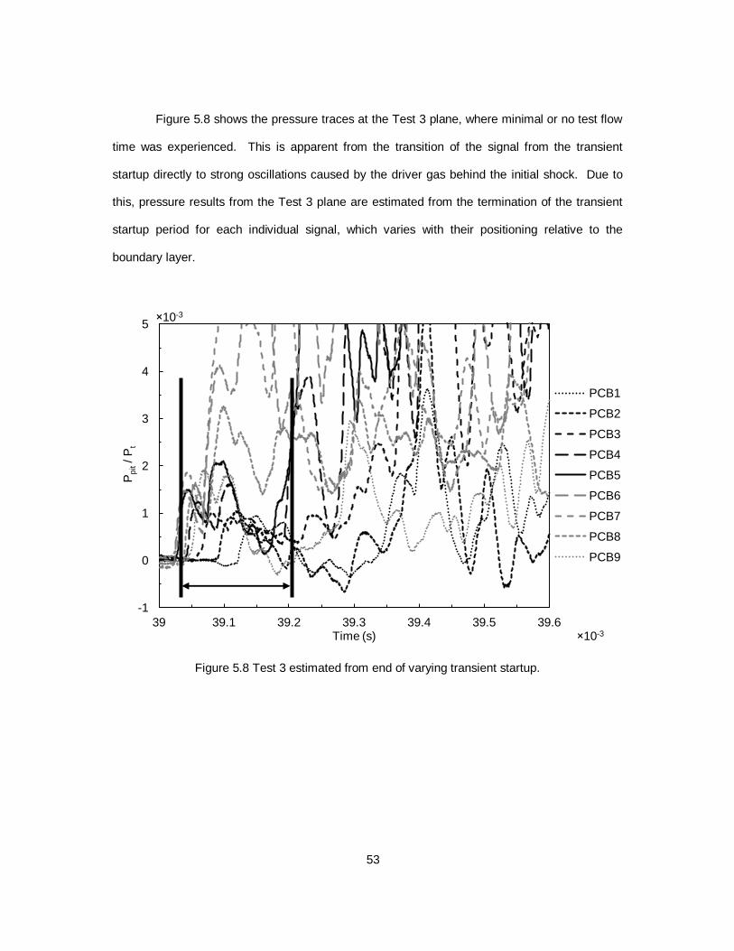
53

Figure 5.8 shows the pressure traces at the Test 3 plane, where minimal or no test flow

time was experienced. This is apparent from the transition of the signal from the transient

startup directly to strong oscillations caused by the driver gas behind the initial shock. Due to

this, pressure results from the Test 3 plane are estimated from the termination of the transient

startup period for each individual signal, which varies with their positioning relative to the

boundary layer.

Figure 5.8 Test 3 estimated from end of varying transient startup.

-1

0

1

2

3

4

5

39 39.1 39.2 39.3 39.4 39.5 39.6

Pp

it / P

t

Time (s)

PCB1

PCB2

PCB3

PCB4

PCB5

PCB6

PCB7

PCB8

PCB9

×10-3

×10-3

54

5.2.3. RTD Response

The voltage output for the single RTD lying near the axial centerline of the tunnel for

each test was processed to determine the stagnation point temperature rise as well as heat flux

under constant and non-constant assumptions.

5.2.3.1 Heat-Flux Determined Via Constant Heat-Flux Case

Voltage responses from the RTD for each test were plotted against the square root of

time and fit with a least-squares linear regression to determine the slope need to calculate heat

flux using a constant heat flux rate assumption. The slope was obtained and used in equation

(4.10) to determine the heat flux for each probe under these ideal circumstances. Some

impedance was experienced in each test case, causing oscillations in the results, as shown in

Figures 5.9 through 5.11. As the heat flux is determined using only the slope of the regression

line, this problem can be mitigated through careful data processing. Also as shown in the same

figure, the selected range of data just after a transient startup period fits a linear approximation

with an adequate correlation and the majority of points falling between two standard deviations

from the regression.

Figure 5.9 Transformed temperature response of RTD 2.

22

26

30

34

38

42

0.1 0.2 0.3 0.4 0.5 0.6 0.7 0.8 0.9 1

Tem

pera

ture

(°C

)

Time1/2 (ms)1/2

Experimental Data

Linear Regression

2σ (95% Confidence)

RTD 2

55

Figure 5.10 Transformed temperature response of RTD 4.

Figure 5.11 Transformed temperature response of RTD 5.

20

25

30

35

40

45

0 0.1 0.2 0.3 0.4 0.5 0.6 0.7 0.8 0.9 1

Tem

pera

ture

(°C

)

Time1/2 (ms)1/2

Experimental Data

Linear Regression

2σ (95% Confidence)

RTD 4

20

24

28

32

36

40

0 0.1 0.2 0.3 0.4 0.5 0.6 0.7 0.8

Tem

pera

ture

(°C

)

Time1/2 (ms)1/2

Experimental Data

Linear Regression

2σ (95% Confidence)

RTD 5

56

5.2.3.2 Heat-Flux Determined Via Cook-Felderman Algorithm

Using the parabolic fit of the response, the data can processed numerically via the

Cook-Felderman algorithm to find the heat flux using a non-constant heat flux assumption. This

time was limited to the first millisecond of data for the Tests 1 and 2 to provide a standard by

which to compare the results between each test plane. Less than one millisecond of useful test

time was present in the response for Test 3 at the back of the test section, most likely due to

degradation of the core flow by the intersecting shocks and expansion waves produced

upstream in the test section. Figures 5.12 through 5.14 show the results of the RTD using the

first millisecond of data with a parabolic fit, except for RTD 5, which only experienced 0.7 ms of

useful data..

Figure 5.12 Temperature response of RTD 2 with transformed regression.

22

26

30

34

38

42

0 0.1 0.2 0.3 0.4 0.5 0.6 0.7 0.8 0.9 1

Tem

pera

ture

(°C

)

Time (s)

Experimental Data

Parabolic Regression

RTD 2

×10-3

57

Figure 5.13 Temperature response of RTD 4 with transformed regression.

Figure 5.14 Temperature response of RTD 5 with transformed regression.

22

26

30

34

38

42

46

0 0.1 0.2 0.3 0.4 0.5 0.6 0.7 0.8 0.9 1

Tem

pera

ture

(°C

)

Time (s)

Experimental Data

Parabolic Regression

RTD 4

22

27

32

37

42

0 0.1 0.2 0.3 0.4 0.5 0.6 0.7

Tem

pera

ture

(°C

)

Time (s)

Experimental Data

Parabolic Regression

RTD 5

58

Equations (4.7a) and (4.7b) can be used with the sensitivities determined during the

static calibration to find a conversion factor to convert the voltage response to surface

temperatures. Results show that the increase in temperature during the test period caused by

the passing shock are fairly minor, increasing by 15-20 °C

Heat flux calculations for the assumed constant and non-constant methods are

tabulated in Table 5.4, including the RTD number used for each test, the duration of the useful

test time used for the Cook-Felderman algorithm, and the estimated error in each reading

caused by the accumulation of errors in each calibration and testing process.

RTD 3 was skipped in the testing process due to electrical burnout while setting up the

Wheatstone bridge circuit immediately preceding Test 1. Error in calculated heat flux was

estimated from the accumulated linearity error of all regression lines used throughout the

calibration and testing data reduction processes.

Table 5.4 Calculated Heat Flux Results

Constant Heat Flux Case (W/cm

2)

Cook-Felderman (W/cm2)

@ [test time] Test RTD

1 4 17.2 ± 11.2% 9.37 ± 8.6% @ t = 1.0 ms

2 2 17.86 ± 10.4% 10.49 ± 8.9% @ t = 1.0 ms

3 5 12.16 ± 10.6% 7.80 ± 5.9% @ t = 0.7 ms

59

CHAPTER 6

CONCLUSIONS AND RECOMMENDATIONS

6.1 Conclusions

All primary objectives of the low enthalpy HST characterization have been completed

successfully, including the design and construction of an apparatus to house pressure and

temperature sensors at three distinct test section planes under approximately the same

operating conditions. A variable length rake and sting system was designed to secure a span

of nine pressure transducers across the test section at these locations, which determined the

pressure and Mach distribution at these planes. From this data and additional shock

calculations, the approximate core flow area was traced.

Platinum thin film RTDs were replicated using a previously documented method.

These sensors were incorporated into the rake design and concurrently recorded stagnation

temperature and heat transfer rates for each test. Results showed that the probe tip surface

temperature increased 15-20 K and the calculated heat flux in the core flow was 9.93 ± 0.56

W/cm2 for the first millisecond of test time.

Due to possible interference at the back of the test section caused by intersecting

oblique shocks and expansion waves generated upstream in the test section, results obtained

at the Test 3 plane are suspect. Future tests should be conducted even with or forward of the

Test 2 plane at the test section midpoint to avoid these flow complications.

60

6.2 Recommendations

To improve the quality of heat flux measurements and reduce the error, a more

automated manufacturing method should be implemented to remove as much human

involvement as possible. Nanofabrication is a quickly growing industry that could suit thin film

applications such as those employed in this study. This would allow for a large number of

nearly identical sensors to be easily replicated and used in great quantities for single tests.

The durability of the thin film sensors must also be addressed. Additional

construction steps to add a highly heat conductive but strong coating material over the films

would greatly increase their durability.

The sting primary and secondary arms can be reused or modified to accommodate a

wide variety of models at any test plane between the Test 1 and Test 3 by simply drilling

additional screw holes. This allows for a 39.37 cm (15.5 in.) axial range of flexibility between

points near the front and back of the test section. Additionally, a rubber O-ring could

potentially be added to the sting interlocking pipe fitting to remove deficiencies in the

connection caused by wear from repeated use.

61

APPENDIX A

RAKE & STING ASSEMBLY AND PART DESIGN

62

63

64

65

66

67

68

69

70

71

72

73

74

75

76

77

78

79

80

81

82

83

84

85

86

APPENDIX B

MATLAB® CODES [15]

87

Sample Low-Pass Butterworth Filter Code Used on Transducer and RTD Output

clc;clear;

fi1 = fopen('Data1.csv'); % input data file f1 = textscan(fi1, '%f %f %f %f %f %f %f %f %f %f', 'Delimiter',

',','HeaderLines',23); fclose(fi1); time =f1{1}; PCB1 =f1{2}; PCB2 =f1{3}; PCB3 =f1{4}; PCB4 =f1{5}; PCB5 =f1{6}; PCB6 =f1{7}; PCB7 =f1{8}; PCB8 =f1{9}; PCB9 =f1{10};

Fs=2500000; % frequency Fc=20000; % filter cutoff frequency cutof_freq= Fc/(Fs/2); [B,A] = butter(1,cutof_freq);

pp1=filter(B,A,PCB1); % filtered vs unfiltered plots pp1=pp1-mean(pp1(1:1000)); plot(time,PCB1) hold on plot(time,pp1,'r')

X = [time,pp1,pp2,pp3,pp4,pp5,pp6,pp7,pp8,pp9]; X = transpose(X); fileID = fopen('Data1.txt','w'); % output text file fprintf(fileID,'%10s %13s %13s %13s %13s %13s %13s %13s %13s

%13s\r\n','TIME','PCB1','PCB2','PCB3','PCB4','PCB5','PCB6','PCB7','PCB

8','PCB9'); fprintf(fileID,'%+9.7f %+10.10f %+10.10f %+10.10f %+10.10f %+10.10f

%+10.10f %+10.10f %+10.10f %+10.10f\r\n',X); fclose(fileID);

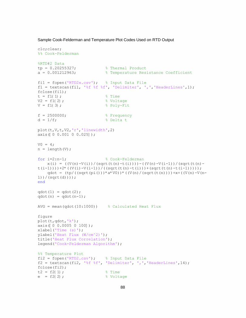
88

Sample Cook-Felderman and Temperature Plot Codes Used on RTD Output

clc;clear; %% Cook-Felderman

%RTD#2 Data tp = 0.20255327; % Thermal Product a = 0.001212963; % Temperature Resistance Coefficient

fi1 = fopen('RTD2x.csv'); % Input Data File f1 = textscan(fi1, '%f %f %f', 'Delimiter', ',','HeaderLines',1); fclose(fi1); t = f1{1}; % Time V2 = f1{2}; % Voltage V = f1{3}; % Poly-Fit

f = 2500000; % Frequency d = 1/f; % Delta t

plot(t,V,t,V2,'r','linewidth',2) axis([0 0.001 0 0.025]);

V0 = 4; n = length(V);

for i=2:n-1; % Cook-Felderman x(i) = ((V(n)-V(i))/(sqrt(t(n)-t(i))))-((V(n)-V(i-1))/(sqrt(t(n)-

t(i-1))))+2*((V(i)-V(i-1))/((sqrt(t(n)-t(i)))+(sqrt(t(n)-t(i-1))))); qdot = (tp/((sqrt(pi()))*a*V0))*((V(n)/(sqrt(t(n))))+x+((V(n)-V(n-

1))/(sqrt(d)))); end

qdot(1) = qdot(2); qdot(n) = qdot(n-1);

AVG = mean(qdot(10:1000)) % Calculated Heat Flux

figure plot(t,qdot,'k'); axis([0 0.0005 0 100]); xlabel('Time (s)'); ylabel('Heat Flux (W/cm^2)'); title('Heat Flux Correlation'); legend('Cook-Felderman Algorithm');

%% Temperature Plot fi2 = fopen('RTD2.csv'); % Input Data File f2 = textscan(fi2, '%f %f', 'Delimiter', ',','HeaderLines',14); fclose(fi2); t2 = f2{1}; % Time e = f2{2}; % Voltage

89

b = 35.179/0.0524; % Deg C/Volts

Fc=20000; % Cutoff Frequency cut= Fc/(f/2); [B,A] = butter(1,cut); % Butterworth Filter

e = (e-mean(e(1:100)))*b+25; e2 = filter(B,A,e);

figure plot(t2,e,t2,e2,'r'); axis([-.0005 0.002 0 70]);

%% Square-Root of Time Linear Regression fi2 = fopen('RTD2y.csv'); % Input Data File f2 = textscan(fi2, '%f %f %f %f %f', 'Delimiter',

',','HeaderLines',14); fclose(fi2); t3 = f2{1}; rtd = f2{2}; lin = f2{3}; % linear fit data con1 = f2{4}; % confidence line data con2 = f2{5}; % confidence line data

figure plot(t3,rtd,'k',t3,lin,'-',t3,con1,'-r',t3,con2,'-g');

90

REFERENCES

1. Stuessy, W. Scott, "Hypersonic Shock Tunnel Development and Calibration," Master's

Thesis, Department of Aerospace Engineering, The University of Texas at Arlington,

Arlington, TX, 1989.

2. Kinnear, Kevin M., "Design, Calibration and Testing of Transient Thin Film Heat Transfer

Gauges," Master's Thesis, Department of Mechanical and Aerospace Engineering, The

University of Texas at Arlington, Arlington, TX, 1997.

3. Anderson, John D., Jr.: Modern Compressible Flow: With Historical Perspective, 3d ed.,

Mcgraw-Hill Book Company, New York, 2003.

4. Chung, Kung-Ming, "Shock Impingement Near Mild Hypersonic Expansion Corners," Ph.D

Dissertation, Department of Aerospace Engineering, The University of Texas at Arlington,

Arlington, TX, 1992.

5. Cone Chart. BigCeramicStore.com. 29 Apr. 2012

<http://www.bigceramicstore.com/information/ConeChart.html>

6. Eckert, E. R. G., and R. M. Drake., Analysis of Heat and Mass Transfer, McGraw-Hill, New

York, 1972.

7. CEARUN. Ed. Dr. Michael J. Zehe. NASA. 22 Mar. 2012 <http://cearun.grc.nasa.gov/>

8. Anderson, John D., Jr., Fundamentals of Aerodynamics, 4th ed., McGraw-Hill, New York,

2007.

9. Reynolds Number. Ed. Tom Benson. 22 May 2009. NASA. 22 Mar. 2012

<http://www.grc.nasa.gov/WWW/BGH/reynolds>

10. Saravanan S., Jagadeesh G., and Reddy K. P. J., "Aerodynamic Force Measurement Using

3-Component Accelerometer Force Balance System in a Hypersonic Shock Tunnel,"

Springer-Verlag, 2008

91

11. Mee, David J., "Dynamic Calibration of Force Balances," Department of Mechanical

Engineering, The University of Queensland, Australia, Report Number 2002/6, 2003.

12. Figliola, R.S. and Beasley, D.E., Theory and Design for Mechanical Measurements, 5th

Edition, John Wiley & Sons, Inc., 2011, pp. 164-168.

13. Cook W. J. and Felderman E. J., "Reduction of Data from Thin-Film Heat-Transfer Gages:

A Concise Numerical Technique," AIAA Journal, Vol. 4, No, 3, 1966, pp.561.

14. Lassaline, J.V., "Supersonic Right Circular Cone at Zero Angle of Attack," Department of

Aerospace Engineering, Ryerson University, Toronto, Ontario, Canada 2009.

15. MATLAB (2008b, The MathWorks, Natick, Massachusetts, U.S.A.)

92

BIOGRAPHICAL INFORMATION

Derek Leamon was born in Dallas, Texas on September 26th, 1984. After developing

an interest in aircraft and spacecraft in high school, he pursued and received a Bachelor of

Science in Aerospace Engineering from The University of Texas at Arlington in 2008. After a

difficult and unrewarding job hunt, Derek returned to UT Arlington a year later seeking higher

education by pursuing a Masters degree from the same department he had left. During his first

year in the Masters program, Derek took multiple Air Breathing Propulsion courses through Dr.

Wilson that led to the opportunity of pursuing an experimentally based thesis in the

Aerodynamics Research Center.