Technische Universität München

Fakultät für Mathematik

M6 Mathematische Modellbildung

Characterizations of Orthogonal Polynomials and

Harmonic Analysis on Polynomial Hypergroups

Stefan Alexander Kahler

Vollständiger Abdruck der von der Fakultät für Mathematik der Technischen UniversitätMünchen zur Erlangung des akademischen Grades eines

Doktors der Naturwissenschaften (Dr. rer. nat.)

genehmigten Dissertation.

Vorsitzende: Prof. Dr. Simone Warzel

Prüfer der Dissertation: 1. Prof. Dr. Rupert Lasser

2. Prof. Dr. Eberhard Kaniuth

3. Prof. Dr. Mourad Ismail

(nur schriftliche Beurteilung)

Die Dissertation wurde am 26.01.2016 bei der Technischen Universität München eingereicht unddurch die Fakultät für Mathematik am 19.04.2016 angenommen.

�God exists since mathematics is consistent, and

the Devil exists since we cannot prove it.�

(André Weil)1

1[GCG98, p. 251]

Abstract

We characterize speci�c classes of orthogonal polynomials in terms of properties which comefrom (or are related to) harmonic and functional analysis such as cohomology. We considerpolynomial hypergroups, which are commutative and come along with a sophisticated harmonicanalysis, and, in the �rst part of the thesis, give a su�cient criterion and a necessary criterion fortheir `1-algebras to be weakly amenable. These criteria will be based on growth and smoothnessconditions, asymptotics, shift operators and various further ingredients such as the Plancherelisomorphism and the fundamental lemma of the calculus of variations. Moreover, we extensivelystudy point amenability (i.e., the nonexistence of nonzero bounded point derivations w.r.t.symmetric characters) w.r.t. such `1-algebras. Both of these amenability notions have beenknown to correspond to certain problems concerning the derivatives of the underlying orthogonalpolynomials�and to be surprisingly rarely satis�ed; the latter contrasts with L1-algebras oflocally compact groups.

Considering suitable ultraspherical polynomials, we show that there exist polynomial hy-pergroups whose `1-algebra is weakly amenable but fails to be (right character) amenable,which solves a problem that has been open for some years. In the second part of the thesis,we completely characterize point and weak amenability for the classes of Jacobi, symmetricPollaczek and associated ultraspherical polynomials (and for two further classes) by identifyingthe corresponding parameter regions. Besides our general criteria, each of these classesrequires speci�c analytical techniques: the characterization concerning the Jacobi polyno-mials makes use of their asymptotics, the Fourier expansions of their derivatives, suitableapproximations and inheritance via homomorphisms. The result for symmetric Pollaczekpolynomials relies on a transformation into a system whose derivatives are more accessibleconcerning asymptotic behavior. Our solution for the associated ultraspherical polynomials willbene�t from a fruitful interplay between hypergeometric and absolutely continuous Fourier series.

The third part of the thesis deals with symmetric, suitably normalized orthogonal polynomialsequences (Pn(x))n∈N0 within which we characterize the class of ultraspherical polynomials interms of certain constancy properties of the Fourier coe�cients belonging to (P ′2n−1(x))n∈N.Such characterizations may be motivated by amenability considerations, and our result improvesprevious work of Lasser�Obermaier in terms of the whole sequence (P ′n(x))n∈N; in fact, weshall uncover some redundancy. We obtain similar characterizations for the discrete and�moreinvolved�continuous q-ultraspherical polynomials via (Dq−1P2n−1(x))n∈N and (DqP2n−1(x))n∈N,respectively, where Dq denotes the q-di�erence operator and Dq denotes the Askey�Wilsonoperator; these characterizations sharpen earlier results of Ismail�Obermaier. Finally, wecharacterize a large subclass of the continuous q-ultraspherical polynomials via the averag-ing operator Aq and explicitly show that this characterization does not extend to the whole class.

Besides these main results, the thesis contains several elaborated motivating examples and addi-tional discussions, recalls important basics, provides background information, and, �nally, brie�yexplains two possible projects w.r.t. postdoctoral research (Outlook).

v

Zusammenfassung

Wir charakterisieren spezi�sche Klassen orthogonaler Polynome über Eigenschaften, welcheaus der harmonischen Analysis und Funktionalanalysis wie der Kohomologie kommen (oderVerwandtschaft dazu aufweisen). Wir betrachten polynomiale Hypergruppen � diese sindkommutativ und gehen mit einer eleganten harmonischen Analysis einher � und präsentierenim ersten Teil der Arbeit ein hinreichendes Kriterium sowie ein notwendiges Kriterium dafür,dass ihre `1-Algebren schwach mittelbar sind. Diese Kriterien gründen auf Wachstums- undGlattheitsbedingungen, asymptotischem Verhalten, Shift-Operatoren und diversen weiterenBestandteilen wie dem Plancherel-Isomorphismus und dem Fundamentallemma der Variation-srechnung. Des Weiteren untersuchen wir ausgiebig Punktmittelbarkeit (d.h. die Nichtexistenznicht-verschwindender beschränkter Punktderivationen bzgl. symmetrischer Charaktere) bzgl.solcher `1-Algebren. Von beiden dieser Mittelbarkeitsbegri�e war bereits bekannt, dass siegewissen Problemstellungen entsprechen, die die Ableitungen der zugrunde liegenden orthog-onalen Polynome betre�en, sowie dass sie überraschend selten erfüllt sind; letzteres steht imKontrast zu L1-Algebren lokalkompakter Gruppen.

Indem wir geeignete ultrasphärische Polynome betrachten, zeigen wir, dass es polynomiale Hy-pergruppen gibt, deren `1-Algebra schwach mittelbar, jedoch nicht (rechts-Charakter-) mittelbarist � was ein Problem löst, dass für einige Jahre o�en gewesen ist. Im zweiten Teil der Arbeitcharakterisieren wir Punktmittelbarkeit und schwache Mittelbarkeit vollständig für die Klassender Jacobi-, symmetrischen Pollaczek- und assoziierten ultrasphärischen Polynome (sowie fürzwei weitere Klassen), indem wir die zugehörigen Parameterregionen identi�zieren. Nebenunseren allgemeinen Kriterien benötigt jede dieser Klassen spezi�sche analytische Techniken:Die die Jacobi-Polynome betre�ende Charakterisierung benutzt deren asymptotisches Verhalten,die Fourier-Entwicklungen ihrer Ableitungen, geeignete Approximationen sowie Vererbung überHomomorphismen. Das Resultat für die symmetrischen Pollaczek-Polynome stützt sich aufeine Transformation in ein System, dessen Ableitungen zugänglicher bzgl. asymptotischenVerhaltens sind. Unsere Lösung für die assoziierten ultrasphärischen Polynome pro�tiert voneinem fruchtbaren Zusammenspiel zwischen hypergeometrischen Reihen und absolut stetigenFourierreihen.

Der dritte Teil der Arbeit befasst sich mit symmetrischen, geeignet normalisierten Folgenorthogonaler Polynome (Pn(x))n∈N0 , innerhalb derer wir die Klasse der ultrasphärischen Poly-nome über gewisse Konstantheitseigenschaften der Fourierkoe�zienten, die zu (P ′2n−1(x))n∈Ngehören, charakterisieren. Solche Charakterisierungen können über Mittelbarkeitsbetrachtungenmotiviert werden. Unser Resultat verbessert ein früheres von Lasser�Obermaier, welches diegesamte Folge (P ′n(x))n∈N in Betracht zog und bzgl. dessen wir eine Redundanz erkennenwerden. Wir erhalten ähnliche Charakterisierungen für die diskreten und � was komplizierter ist� kontinuierlichen q-ultrasphärischen Polynome über (Dq−1P2n−1(x))n∈N bzw. (DqP2n−1(x))n∈N,wobei Dq den q-Di�erenzenoperator und Dq den Askey�Wilson-Operator bezeichnet; dieseCharakterisierungen verschärfen frühere Resultate von Ismail�Obermaier. Schlussendlichcharakterisieren wir eine groÿe Teilklasse der kontinuierlichen q-ultrasphärischen Polynomeüber den Averaging-Operator Aq und zeigen explizit, dass diese Charakterisierung nicht für diegesamte Klasse gilt.

Neben diesen Hauptresultaten enthält die Arbeit mehrere ausgearbeitete motivierende Beispieleund zusätzliche Diskussionen, wiederholt wichtige Grundlagen, stellt Hintergrundinformationenzur Verfügung und erklärt abschlieÿend kurz zwei mögliche Projekte mit Blick auf Postdoktoran-denforschung (Outlook).

vi

List of publications

This thesis is a publication-based dissertation, based on our papers [Kah15] and [Kah16].

� Our paper �Orthogonal polynomials and point and weak amenability of `1-algebras ofpolynomial hypergroups� [Kah15] was �rst published in Constructive Approximation in

Constr. Approx. 42 (2015), no. 1, 31�63,DOI: http://dx.doi.org/10.1007/s00365-014-9246-2,

published by Springer Science+Business Media New York. The author respects the �Copy-right Transfer Statement� which can be found in the appendix of this thesis. Springer holdsthe copyright of [Kah15]. However, the �Copyright Transfer Statement� explicitly permitsthe author to include the �nal published journal article in other publications (such as hisdissertation).

� Our paper �Characterizations of ultraspherical polynomials and their q-analogues� [Kah16]was �rst published in Proceedings of the American Mathematical Society in

Proc. Amer. Math. Soc. 144 (2016), no. 1, 87�101,electronically published on September 4, 2015, DOI: http://dx.doi.org/10.1090/proc/12640(to appear in print),

published by American Mathematical Society. The author electronically signed the �Con-sent to Publish� which can be found in the appendix of this thesis. The American Mathe-matical Society holds the copyright of [Kah16]. However, the �Consent to Publish� explicitlypermits the author to use (part or all of) the work in his own future publications.

Both papers can be found in the appendix.

The author gratefully acknowledges the possibility provided by Springer Science+BusinessMedia New York to include [Kah15] in his dissertation.

The author gratefully acknowledges the possibility provided by the American MathematicalSociety, Providence, RI to include [Kah16] in his dissertation.

Due to the publication-based character, parts of this thesis are very similar to our papers [Kah15,Kah16].

vii

Preface and acknowledgments

This work is located at a crossing point between the branches of functional, harmonic and Fourieranalysis on the one hand, and the theory of orthogonal polynomials and special functions onthe other hand. The focus of our research can be divided into three parts, contained in threecorresponding main sections:

� Part I: general results on weak amenability�and on the nonexistence of nonzero boundedpoint derivations w.r.t. symmetric characters�concerning `1-algebras of polynomial hy-pergroups (on N0); weak amenability for `1-algebras corresponding to ultraspherical poly-nomials, and the solution to the (previously open) problem whether it is possible that aweakly amenable `1-algebra of a polynomial hypergroup fails to be amenable. See Section 2and [Kah15].

� Part II: weak amenability�and the nonexistence of nonzero bounded point derivations�for `1-algebras corresponding to important one-parameter generalizations of the ultraspher-ical polynomials (Jacobi, symmetric Pollaczek, associated ultraspherical). See Section 3and [Kah15].

� Part III: new characterizations of ultraspherical, discrete q-ultraspherical and continuousq-ultraspherical polynomials in terms of the derivative, the q-di�erence operator Dq andthe Askey�Wilson operator Dq, respectively; new characterization of certain continuousq-ultraspherical polynomials in terms of the averaging operator Aq�and the proof thatthe latter characterization does not hold for the whole class of continuous q-ultrasphericalpolynomials. See Section 4 and [Kah16].

The main (and most of the further) results of this thesis can be found in the papers[Kah15, Kah16]; however, the thesis contains also a few results which are not contained in thepapers. For instance, the notes at the end of Section 4.4 are a sharpening of the correspondingparts in [Kah16]. Furthermore, in Section 3 we now also consider the notions of α-amenability(or, closely related, ϕ-amenability) and right character amenability (without exception, thecorresponding situations w.r.t. amenability itself are easier to see and have been known before).Concerning an important step in the proof of Theorem 3.2 (which is also [Kah15, Theorem 4.1]),we present a faster yet less elementary variant, see Remark 3.1.

The thesis contains several detailed �motivating examples�: Section 2.1 reconsiders weakamenability for the �minimal� (but nevertheless interesting) example of the Chebyshev poly-nomials of the �rst kind and discusses arising problems, which motivates our su�ciencycriterion Theorem 2.1 [Kah15, Theorem 2.3]. Via an estimation using Dougall's formula, theasymptotic behavior of the gamma function, the power mean inequality and the Riemannzeta function, Section 2.5 applies this su�ciency criterion to the ultraspherical polynomialscorresponding to the parameter region properly between the Chebyshev polynomials of the�rst kind and the Legendre polynomials. On the one hand, this provides �rst examples ofpolynomial hypergroups whose `1-algebra is weakly amenable but fails to be amenable. Infact, we will even obtain simultaneous failure of right character amenability. On the otherhand, Section 2.5 motivates the considerably more involved approach for Theorem 3.1 [Kah15,Theorem 3.1] on general Jacobi polynomials. Section 3.1 applies our necessary criterion forweak amenability, Theorem 2.2 [Kah15, Theorem 2.2], to the �non-ultraspherical� subclass ofthe symmetric Pollaczek polynomials in a rather elementary way (via Euler's in�nite productformula for the complex gamma function, elementary approximation and Stirling's formula).This result is then improved in Theorem 3.2 towards establishing even the existence of a nonzerobounded point derivation. Furthermore, it motivates the similar yet no longer elementarystudy of the associated ultraspherical polynomials leading to Theorem 3.3 [Kah15, Theorem 5.1].

viii

With few exceptions, what cannot be found in the main sections of this thesis are the detailedproofs. Concerning the latter, we explicitly refer to our papers�in which the details are given.Our motivation for writing Section 2, Section 3 and Section 4 was a twofold one: on the onehand, the purpose is to provide a thorough overview, including elaborated motivations for ourresults (and for our research at all), some background and also some additional information�allof this in a more extensive way than this would have been possible in the paper versions. Onthe other hand, the purpose is to achieve a concise presentation which is limited to outlinesor sketches of those proofs that can be found in the papers [Kah15] and [Kah16] (which areincluded in this publication-based dissertation).

The introductory Section 1 starts with the Banach�Tarski paradox and Tarski's theorem ashistorical motivation for amenability considerations and recalls some of the most importantamenability notions for groups, hypergroups and�most important for our purposes�Banachalgebras: we particularly recall the notions of amenability (Johnson), weak amenability (Bade�Curtis�Dales and Johnson), right character amenability (Kaniuth�Lau�Pym and Monfared)and point amenability (nonexistence of nonzero bounded point derivations w.r.t. symmetriccharacters, regarded as a global property). We also recall the most important facts about(polynomial) hypergroups and their basic harmonic analysis. Very roughly speaking, the maindi�erence between a group and the more general notion of a hypergroup is that the convolutionof two Dirac measures need no longer be a Dirac measure again but still a (more general)probability measure in the latter case; the algebraic group operations are generalized to thehypergroup convolution and involution, which are required to satisfy certain compatibilityand non-degeneracy properties. Polynomial hypergroups on N0 were introduced by Lasser inthe 1980s, have a sophisticated harmonic analysis and provide a very rich example class. Forthe L1-algebra of a locally compact group G, amenability and right character amenability areknown to correspond to the amenability of G (where Johnson's characterization �G amenable⇔ L1(G) amenable� can be regarded as basic motivation to consider amenability notions forBanach algebras), whereas weak amenability and point amenability are always satis�ed. Forthe `1-algebra of a polynomial hypergroup, however, the situation is very di�erent: althougheach polynomial hypergroup is known to be amenable in the hypergroup sense, even pointamenability of the `1-algebra, which is the weakest of the four abovementioned properties forBanach algebras, is often not satis�ed. Furthermore, the individual behavior strongly dependson the inducing sequence (Pn(x))n∈N0 of orthogonal polynomials (or on the orthogonalizationmeasure µ) and can quickly lead to major challenges in the theory of orthogonal polynomialsand special functions. A very convenient criterion of Lasser (2007) states that the `1-algebraof a polynomial hypergroup necessarily fails to be amenable whenever the Haar weights tendto in�nity. This allows to rule out amenability for most of the naturally occurring exam-ples. Also for right character and point amenability convenient criteria have been available;concerning point amenability, there is a criterion of Lasser (2009) which relates the existenceof nonzero bounded point derivations to the derivatives of the underlying orthogonal polynomials.

For weak amenability, however the situation has been much worse: even for ultrasphericalpolynomials (P

(α)n (x))n∈N0 , which for α ≥ −1

2 form the surely most prominent example classfor polynomial hypergroups, the situation has been open for the parameter region properlybetween the Chebyshev polynomials of the �rst kind and the Legendre polynomials (i.e., forα ∈

(−1

2 , 0); as already mentioned above, we will give the solution in Section 2.5). Moreover,

there has not been a convenient criterion for weak amenability. A characterization of Lasser(2007) in terms of the Fourier coe�cients2 of the (inducing polynomials') derivatives, whichwill be precisely recalled in Section 1.4, has su�ered from several general barriers (such as therequirement of deep�and frequently not explicitly available�knowledge about the inducing

2`Fourier coe�cients' means coe�cients in expansions w.r.t. the basis{

1∫RP

2n(x) dµ(x)

Pn(x) : n ∈ N0

}.

ix

orthogonal polynomials, and the requirement to deal with the whole space `∞, despite the factthat many of the powerful tools of harmonic analysis are restricted to proper subspaces). Ithas also su�ered from a lack of applicability: to our knowledge, its su�cient direction has beensuccessfully applied only to examples where also the stronger notion of amenability holds (e.g.,to the Chebyshev polynomials of the �rst kind), and its necessary direction has been successfullyapplied only to examples where the structure of the underlying orthogonal polynomials is veryspeci�c and allows for explicit computations (e.g., to the ultraspherical polynomials for α ≥ 0)or where one might also argue via point derivations instead (e.g., ultraspherical polynomials forα ≥ 1

2). The two main results of Section 2 are our su�ciency criterion and our necessary criterionmentioned above, which are both based on Lasser's characterization but overcome the describedproblems in a satisfying way: the su�cient criterion Theorem 2.1 relies on limiting behaviorof orthogonal polynomials, growth conditions, the Plancherel isomorphism and several furtheringredients such as the fundamental lemma of the calculus of variations, and its combinationwith inheritance via homomorphisms will turn out to be strong enough to establish weakamenability whenever this property occurs in the whole classes of Jacobi, symmetric Pollaczekand associated ultraspherical polynomials. The necessary criterion Theorem 2.2 relies on shiftoperators and shows that the `1-algebra cannot be weakly amenable if the orthogonalizationmeasure does not behave su�ciently �badly�. It will essentially contribute to ruling out weakamenability when this property fails in the three just mentioned classes. Section 2 provides alsohelpful results concerning point amenability of `1-algebras of polynomial hypergroups.

Theorem 3.1, Theorem 3.2 and Theorem 3.3 are the main results of Section 3. They providethe following characterizations, which are full descriptions of point and weak amenability for theclasses of Jacobi, symmetric Pollaczek and associated ultraspherical polynomials:

� The `1-algebra induced by the Jacobi polynomials (R(α,β)n (x))n∈N0 is point amenable if and

only if α < 12 , and weakly amenable if and only if α < 0.

� The `1-algebra induced by the symmetric Pollaczek polynomials (Q(α,λ)n (x))n∈N0 is point

amenable if and only if α < 12 and λ = 0, and weakly amenable if and only if α < 0 and

λ = 0.

� The `1-algebra induced by the associated ultraspherical polynomials (A(α,ν)n (x))n∈N0 is

point amenable if and only if α < 12 , and weakly amenable if and only if α < 0 and ν = 0.

Concerning the general regions from which the parameters are taken such that a polynomialhypergroup is induced, and concerning earlier partial results, we refer to Section 3. Besidesapplications of general results of Section 2, establishing these characterizations requires speci�canalytical techniques for each of the three classes. The Jacobi polynomials are tackled via theChu�Vandermonde and the Pfa��Saalschütz identity, the Stolz�Cesàro theorem, a technicalinduction argument and inheritance via homomorphisms, and via their asymptotics. In contrastto the purely ultraspherical case considered in Section 2.5, explicit computations seem to berather impracticable at some stages�and it will be one of our tasks to avoid them as far aspossible. Our proof concerning point amenability for the symmetric Pollaczek polynomials isessentially based on a transformation into a system with easier asymptotic behavior, and ona subsequent estimation of the derivatives at 0. While, for instance, the Jacobi polynomialscan be represented as a terminating 2F1 hypergeometric series in a rather convenient way,such estimations are much more involved for the symmetric Pollaczek polynomials (for whichexpedient explicit computations seem to be out of reach�for instance, in the hypergeometricrepresentation of the symmetric Pollaczek polynomials, x occurs both in the argument andin a parameter). Our result on the associated ultraspherical polynomials is based on Euler'stransformation for hypergeometric functions, on the location of the zeros of hypergeometricfunctions, on Pringsheim's theorem and on an own result concerning absolute continuity ofFourier series (which might be of interest of its own). Another important generalization of

x

the ultraspherical polynomials, namely the class of continuous q-ultraspherical (or Rogers)polynomials, has already been known to contain no example such that `1(h) is at least pointamenable. Finally, in Section 3.5 we study two further classes (random walk polynomials andcosh-polynomials). We note at this stage that two auxiliary results, namely Lemma 2.4 (i) andLemma 3.1, can also be found in the author's Master's thesis [Kah12] (the latter with a di�erentproof, however).

Theorem 3.1, Theorem 3.2 and Theorem 3.3 can also be seen as characterizations of certain(subclasses of classes of) orthogonal polynomials. Characterizing speci�c orthogonal polyno-mials has a long history. Section 4 is devoted to another type of such characterizations: asalready mentioned above, the Fourier coe�cients of the derivatives of the underlying orthogonalpolynomials play a crucial role with regard to weak amenability of `1-algebras of polynomialhypergroups. The simpli�cation of the proof of Theorem 3.1 when restricting oneself to thepurely ultraspherical subcase (as presented in the motivating Section 2.5) is partially reasonedin the very simple form these Fourier coe�cients take for the ultraspherical polynomials; a moredetailed discussion is given in Section 4.1. In fact, this simple form, a striking constancy prop-erty, characterizes the ultraspherical polynomials: in 2008, Lasser and Obermaier found thatfor a sequence (Pn(x))n∈N0 of symmetric random walk polynomials3 with normalization pointA > 0 (i.e., Pn(A) = 1 (n ∈ N0)) and orthogonalization measure µ the following are equivalent:

(i) Pn(x) = P(α)n (x) (n ∈ N0) for some α > −1, (ii) A = 1 and P ′n(x) = P ′n(1)P ∗n−1(x) (n ∈ N).

Here, (P ∗n(x))n∈N0 is the random walk polynomial sequence w.r.t. the normalization point Aand the measure dµ∗(x) := (A2 − x2) dµ(x) (which is well-de�ned because supp µ ⊆ [−A,A] forsymmetric random walk polynomial sequences). The condition P ′n(x) = P ′n(1)P ∗n−1(x) (n ∈ N)is a concise reformulation of the aforementioned constancy property of the Fourier coe�cients.

This result by Lasser and Obermaier has experienced improvements in two directions: on the onehand, in 2011 Ismail and Obermaier found analogues for the classes of discrete and continuousq-ultraspherical polynomials (later, Ismail and Simeonov obtained also extensions to symmetricAl-Salam�Chihara, symmetric Askey�Wilson and symmetric Meixner�Pollaczek polynomials,and the author's Master's thesis [Kah12] contains suitable extensions to the classes of Jacobiand generalized Chebyshev polynomials); the characterization of the discrete q-ultrasphericalpolynomials (Pn(x;α : q))n∈N0 uses the q-di�erence operator Dq (more precisely, Dq−1), andthe characterization of the continuous q-ultraspherical polynomials (Pn(x;β|q))n∈N0 is in termsof another q-generalization of the classical derivative, namely in terms of the Askey�Wilson

operator Dq (q ∈ (0, 1); α, β ∈(

0, 1√q

)). On the other hand, we have shown in our Master's

thesis [Kah12] that the Lasser�Obermaier characterization remains valid if (ii) is replaced bythe apparently weaker condition �A = 1 and P ′2n−1(x) = P ′2n−1(1)P ∗2n−2(x) (n ∈ N)�. In fact, itsu�ces to require a constancy property as described above only for odd indices and only at somecarefully chosen points. In contrast to the original Lasser�Obermaier result, this sharpeningdoes no longer follow from older, more �classical� results of Hahn and Al-Salam�Chihara.

Theorem 4.4 [Kah16, Theorem 2.1] is a modi�cation of the just mentioned result of our Master'sthesis [Kah12]: Theorem 4.4 is no longer restricted to random walk polynomials but considersmore general (symmetric) orthogonal polynomial sequences (Pn(x))n∈N0 . Since this more generalsetting does no longer contain a condition which a priori enforces that supp µ ⊆ [−A,A] (or theboundedness of supp µ, or at least the uniqueness of µ, at all), it also requires a more generalinterpretation of the sequence (P ∗n(x))n∈N0 . Since this improvement does not a�ect the actualproof, however, we shall mainly focus on the classes of discrete and continuous q-ultrasphericalpolynomials in Section 4: the main purpose is to sharpen the Ismail�Obermaier results on the

3In this thesis, the expression �random walk polynomials� will be used with two di�erent meanings: the currentmeaning, which corresponds to that in Section 4, di�ers from the meaning in Section 3.

xi

discrete and continuous q-ultraspherical polynomials in the same way as we have been ableto sharpen the Lasser�Obermaier result on purely ultraspherical polynomials in our Master'sthesis [Kah12] and in Theorem 4.4; such a project (as part of the author's dissertation) wasannounced in the outlook of [Kah12]. In this context, the two main results are Theorem 4.5[Kah16, Theorem 2.2] and Theorem 4.6 [Kah16, Theorem 2.3].

While Theorem 4.5 (discrete q-ultraspherical polynomials) can be established via an inductionargument that resembles the proof of Theorem 4.4 (ultraspherical polynomials), Theorem 4.6(i.e., the analogous characterization of the continuous q-ultraspherical polynomials) requiresadditional and more sophisticated strategies. The actual reason for the more technical andinvolved argument is that while the product formula for the q-di�erence operator basicallyresembles that of the classical derivative, the product formula for the Askey�Wilson operatoressentially relies on an additional operator Aq, an averaging operator. This leads to the problemthat one has to simultaneously tackle (determinacy problems concerning) the additional Fouriercoe�cients w.r.t. this averaging operator. An important idea to overcome this problem is toconsider the functions n 7→ Aq[xPn(x)] and determinacy of corresponding Fourier coe�cients.Moreover, our proof will rely on a detailed study and some kind of �simultaneous involvement�of the continuous q-ultraspherical polynomials themselves; the latter yields a conclusion whichavoids further tedious calculations and considerably shortens the argument.

The fourth main result of Section 4, Theorem 4.7 [Kah16, Theorem 2.4], is a characterization ofthe continuous q-ultraspherical polynomials with β ≤ 1 in terms of the averaging operator Aq.Provided q ∈ (0, 1), β ∈ (0, 1], Pn

(√β

2 + 12√β

)= 1 (n ∈ N0) and P2(0) = −β 1−q

1−β2q, it yields the

equivalence of the following two properties:

(i) Pn(x) = Pn(x;β|q) (n ∈ N0),

(ii) the quotient∫RAqPn+1(x)Pn−1(x) dµ(x)∫RDqPn+1(x)Pn(x) dµ(x)

is independent of n ∈ N.

Again, this will be shown via an induction argument. The second part of Theorem 4.7 statesthat this characterization does not hold for the whole class of continuous q-ultrasphericalpolynomials; more precisely, the characterization becomes wrong if the condition �β ∈ (0, 1]�

is replaced by the weaker condition �β ∈(

0, 1√q

)� (which worked in Theorem 4.6). We will

establish an explicit counterexample based on the sequence(Pn(x; 5

4

∣∣12

))n∈N0

.

The thesis concludes with a short outlook on possible future research, with a collection ofimportant symbols, with the appendix�which, besides the papers [Kah15, Kah16] with thedetailed proofs, the Springer �Copyright Transfer Statement� and the AMS �Consent to Publish�,includes summaries of the papers�and, �nally, with the references. The BibTeX code of mostof the references was taken from the AMS website (MathSciNet), often with slight adjustments.

Apart from pointing out relations to own works, we deliberately refrain from giving referencesin a preface; however, the precise references will be given in the later parts of this thesis.

In the course of our research, we have frequently used mathematical software (Maple)�to getideas and conjectures, observe possible simpli�cations, identify possible asymptotic and limitingor growth behavior, get an idea of numerical values, �check� calculations, plot graphs and so on.Since we think that it is reasonable and standard in modern mathematics to use such valuableauxiliary tools for the described purposes, we will refrain from pointing out the single usagesin this thesis. However, we want to emphasize that such mathematical software is not neededto understand the �nal proofs. The thesis, including our papers [Kah15, Kah16], can be readwithout any computer usage; in particular, long calculations have been simpli�ed so far thatthey do not require a computer algebra system and can be made by hand (in reasonable time).

xii

Acknowledgments

I �rst want to express my gratitude to Prof. Dr. Rupert Lasser for encouraging me to doresearch in this beautiful �eld of mathematics, for many interesting and fruitful discussions,and for an always open door. I also want to express my gratitude to him for supporting myparticipation in six international conferences and encouraging me to contribute talks to them(which brought me to places like Kaohsiung, Hong Kong, Tianjin and Granada), for attendingseveral of these conferences together, and for supporting my participation in a summer schoolat Lisbon. Prof. Lasser taught me in measure theory, functional analysis and many furtherareas of mathematics when I was a student, and his lectures sharpened my mathematical viewand rigor. Later, he became my TopMath mentor and doctorate supervisor, and I am gratefulfor the chance to work together with him.

Since I �rst met him at an �Abstract Harmonic Analysis� conference in Kaohsiung, Prof. Dr.Eberhard Kaniuth has been showing continuous interest in my research and my scienti�c way.Prof. Kaniuth supported my participation in further conferences of the �Abstract HarmonicAnalysis� series and always gave me the feeling to be a member of the community. I also wantto thank him for taking the time to meet and discuss during several of his visits in Munich.

I had the chance to meet Prof. Dr. Mourad E.H. Ismail at a conference on asymptotics andspecial functions in Hong Kong, and I am thankful for the interest he has shown in my research.

I want to thank Prof. Dr. Martin Brokate, who is my mentor w.r.t. TUM Graduate School,and his secretary Birgit Viehl. Prof. Brokate has always had an open door for me, and I amgrateful for the possibility to use a room at his chair M6. I want to thank Prof. Dr. GeroFriesecke, who was my TopMath mentor in the �rst TopMath years, for bringing me into�rst contact with mathematical research�including the chance to participate in a workshopat Oberwolfach. Prof. Friesecke taught me analysis when I was a young student, and I amgrateful for the mathematical intuition he imparted in his lectures and in discussions. I amgrateful for the interest concerning my research PD Dr. Josef Obermaier has been showing formany years. Many thanks to my neighbor and former fellow student Dr. Robert Lang�notonly for reading parts of the manuscript of this thesis, but also for an abundance of �scienti�cevenings� from Gödel to string theory etc.; I am grateful for our good and reliable friendship,which has accompanied me for more than ten years now and which has given us the possibilityto learn from each other. I want to express my gratitude to my former fellow student Dr. YuenAu Yeung, both for his advice concerning many (non-mathematical) topics of life and for hisfriendship. Many thanks also to my former fellow student Dr. Peter Heinig�for reading an earlyversion of [Kah15], and for his friendship. Moreover, I am indebted to Dr. Peter Heinig, Dr.Robert Lang and my former fellow student Felix Früchtl for listening to drafts of conference talks.

I gratefully acknowledge support from the graduate program TopMath of the ENB (EliteNetwork of Bavaria) and the TopMath Graduate Center of TUM Graduate School at TechnischeUniversität München. During large parts of my research I was partially supported by ascholarship from the Max Weber-Programm within the ENB and by a scholarship from theStudienstiftung des deutschen Volkes.

Neither my studies nor my research would have been possible without the everlasting supportand love of my family. I want to express my deepest gratitude to my family, and also to myfriends!

xiii

Contents

Abstract and list of publications v

Preface and acknowledgments viii

1. From the Banach�Tarski paradox to amenability notions for hypergroups and orthog-onal polynomials 11.1. Historical motivation . . . . . . . . . . . . . . . . . . . . . . . . . . . . . . . . . . 11.2. Amenability notions for groups and Banach algebras . . . . . . . . . . . . . . . . 31.3. Hypergroups and orthogonal polynomials: some basic harmonic analysis . . . . . 71.4. Hypergroups and orthogonal polynomials: various types of amenability . . . . . . 13

2. Point and weak amenability of `1-algebras of polynomial hypergroups: general results 192.1. Motivating example: Chebyshev polynomials of the �rst kind reconsidered . . . . 192.2. Establishing weak amenability: growth conditions and asymptotics . . . . . . . . 212.3. Ruling out weak amenability: shift operators and smoothness conditions . . . . . 232.4. Inheritance via homomorphisms and results on point amenability . . . . . . . . . 252.5. A �rst application of the su�cient criterion: ultraspherical polynomials and the

solution to the problem �amenability vs. weak amenability� . . . . . . . . . . . . 26

3. Complete characterizations of point and weak amenability for speci�c classes 293.1. A �rst application of the necessary criterion: weak amenability and smoothness

for symmetric Pollaczek polynomials . . . . . . . . . . . . . . . . . . . . . . . . . 313.2. Jacobi polynomials: transition from the purely ultraspherical case, and how to

avoid dealing with a 9F8 . . . . . . . . . . . . . . . . . . . . . . . . . . . . . . . . 333.3. Symmetric Pollaczek polynomials: transformations and estimations of the deriva-

tives . . . . . . . . . . . . . . . . . . . . . . . . . . . . . . . . . . . . . . . . . . . 363.4. Associated ultraspherical polynomials: interplay between hypergeometric and ab-

solutely continuous Fourier series . . . . . . . . . . . . . . . . . . . . . . . . . . . 393.5. Further classes: random walk polynomials and cosh-polynomials . . . . . . . . . . 41

4. Characterizations of ultraspherical and q-ultraspherical polynomials 444.1. Weak amenability reconsidered and a characterization of ultraspherical polynomials 444.2. A characterization of discrete q-ultraspherical polynomials in terms of the q-

di�erence operator . . . . . . . . . . . . . . . . . . . . . . . . . . . . . . . . . . . 504.3. A characterization of continuous q-ultraspherical polynomials in terms of the

Askey�Wilson operator . . . . . . . . . . . . . . . . . . . . . . . . . . . . . . . . . 524.4. A characterization of continuous q-ultraspherical polynomials in terms of the av-

eraging operator . . . . . . . . . . . . . . . . . . . . . . . . . . . . . . . . . . . . 56

Outlook 58

Symbols 62

A. Publication [Kah15] 67A.1. Summary . . . . . . . . . . . . . . . . . . . . . . . . . . . . . . . . . . . . . . . . 67A.2. �Copyright Transfer Statement� Springer and included publication . . . . . . . . 68

B. Publication [Kah16] 107B.1. Summary . . . . . . . . . . . . . . . . . . . . . . . . . . . . . . . . . . . . . . . . 107B.2. �Consent to publish� AMS and included publication . . . . . . . . . . . . . . . . . 108

References 127

xv

1. From the Banach�Tarski paradox to amenability notions forhypergroups and orthogonal polynomials

Parts of Section 1 are very similar to our publication [Kah15].

1.1. Historical motivation

In 1924, Banach and Tarski found a result which has become famous far beyond the mathe-matical community: a ball in R3 can be split into a �nite number of pieces in such a way thatthese pieces can be reassembled into two balls of the original size; more generally, given any twobounded sets A,B ⊆ R3 with nonempty interior, it is possible to split A into �nitely many piecesand rearrange them to a partition of B, using nothing but rigid motions. In his foreword to[Wag93], Mycielski calls this `Banach�Tarski paradox' the �most surprising result of theoreticalmathematics� [Wag93, p. xi]. Without any doubt, it is indeed counterintuitive from a physicalpoint of view, more precisely: it strikingly shows that a mathematical result, in particular ahighly nonconstructive one (in 1964, Solovay showed that the Banach�Tarski paradox is notcontained in ZF or at least in ZF + DC, i.e., ZF + the `axiom of dependent choice', cf. [Wag93,Chapter 13]), may be far away from being compatible with �everyday experience�, and only ofnarrow signi�cance concerning physical theories. From a purely mathematical point of view,the (very subjective) question whether one �nds the Banach�Tarski paradox surprising or notmay be related to the personal attitude towards the axiom of choice (which, due to Gödel andCohen, is logically independent of ZF): the constructivist might argue that a counterintuitive,or even �unnatural�, axiom should not be expected to produce intuitive theorems, whereasthe formalist, or the �pragmatic� analyst who bene�ts from the Hahn�Banach theorem, fromAlaoglu's theorem and from many other results and concepts which would not be available inZF, has to (and will) approve that his kind of mathematics intrinsically enforces phenomenalike the Banach�Tarski paradox (and, in particular, sets which are not Lebesgue-measurable).Across all factions, however, it should be quite unexpected that�despite the generalizationsto n dimensions, n ≥ 4, are valid [Wag93, Chapter 5]�the Banach�Tarski paradox has noanalogue in R or R2; this is a consequence of Banach's theorem (1923) which shows that theLebesgue-measures on R and R2 extend to isometry-invariant �nitely additive measures onP(R) and P(R2), respectively [Wag93, Corollary 10.9].

The proof of the Banach�Tarski paradox is easier than one might expect; a very readable version,which does not necessarily require to deal with the extensive background theory, can be foundin the �rst three chapters of [Wag93]. A very helpful tool is the concept of `paradoxical sets' and`paradoxical groups':

De�nition. Let X be a set, and let G be a group that acts on X. Then a subset E of X iscalled `G-paradoxical' if there exist a partition {A1, . . . , Am, B1, . . . , Bn}, m,n ∈ N, of E anda1, . . . , am, b1, . . . , bn ∈ G such that as well {a1(A1), . . . , am(Am)} as {b1(B1), . . . , bn(Bn)} is apartition of E. G itself is called `paradoxical' if G is G-paradoxical w.r.t. the left translations.

With this de�nition, the Banach�Tarski paradox�from now on, we refer to the three-dimensional�standard form� (two balls out of one), and not to the �strong form� (arbitrary bounded sets withnonempty interior)�reads as follows: every ball in R3 is G3-paradoxical, where G3 denotes theisometry group of R3. The central part of the proof given in [Wag93] is the following ingredient[Wag93, Proposition 1.10]:

Proposition 1.1. Let X be a set, and let G be a paradoxical group that acts freely (i.e., withoutnontrivial �xed points) on X. Then X is G-paradoxical.

In the proof of Proposition 1.1, the axiom of choice is needed to obtain a partition {g(N) : g ∈ G}of X, where N ⊆ X and the G-orbits in X intersect at single points; such a�highly

1

nonconstructive��coordinate system�, consisting of the orbits on the one hand and the imagesof N under the group action on the other hand, allows to transfer a �paradoxical decomposition�of G to a paradoxical decomposition of X. Based on Proposition 1.1, in [Wag93] the remainingproof of the Banach�Tarski paradox is done via a speci�c paradoxical subgroup of SO(3) (a freegroup of rank 2; partially going back to von Neumann), via the resulting `Hausdor� paradox' forspheres, via an argument which goes back to Sierpi«ski and makes it possible to handle groupactions with at last countably many �xed points and, �nally, via the transition from spheresto balls (and the Banach�Schröder�Bernstein theorem if one is interested in the strong form).Roughly speaking, the overall approach is to obtain a rather explicit decomposition w.r.t. highlynon-explicit �coordinates� provided by the axiom of choice.

Being older than 90 years now, the Banach�Tarski paradox has experienced many (deep)improvements. In 1991, Pawlikowski proved that the Banach�Tarski paradox is already impliedby the Hahn�Banach theorem [Paw91], which is well-known to be weaker than the axiom ofchoice (and which is also weaker than Alaoglu's theorem [Lux62, Lux69, Pin72]�Alaoglu'stheorem is known to be still weaker than the axiom of choice [HL71, Lux69]; cf. also [Edw75]).Much earlier results concern minimizing the number of necessary pieces in the decomposition(in 1947, Robinson showed that �ve pieces are enough yet also necessary, cf. [Wag93, Chapter4]) and in�nite versions (even getting a continuum of spheres from one, Sierpi«ski 1945, cf.[Wag93, Chapter 6]). In 1994, Dougherty and Foreman gave a decomposition using pieceswhich have the property of Baire (solution to Marczewski's problem) [DF94]. In 2005, Wilsonestablished a continuous movement version (solution to de Groot's problem) [Wil05]. Moreover,the lack of analogues in one or two dimensions suggested another eye-catching question whichbecame known as Tarski's circle-squaring problem and was answered positively by Laczkovichin 1990: it is possible to cut a disc into �nitely many pieces and rearrange them to a square(of necessarily the same area) [Lac90]. Laczkovich's proof uses the axiom of choice and about1050 pieces, and it shows that the rearrangement can even be done by using only translations;again there is a recent continuous movement version [Wil05]. Related results are the�mucholder�von Neumann paradoxes for the plane and line, see [Wag93, Chapter 7].

More important for our purposes, however, is Tarski's theorem: In the light of the Banach�Tarski paradox and Banach's theorem, it is an interesting question how the (non)existence ofparadoxical decompositions is related to the existence of �nitely additive measures. The answerwas given by Tarski in 1938 [Wag93, Corollary 9.2]:

Theorem 1.1 (Tarski's theorem). Let X be a set, let G be a group that acts on X, and let Ebe a subset of X. The following are equivalent:

(i) E is not G-paradoxical,

(ii) there exists a G-invariant �nitely additive measure ν : P(X)→ [0,∞] with ν(E) = 1.

Of course, the nontrivial direction is �(i) ⇒ (ii)�. Applying Theorem 1.1 to G itself (and theaction via left translations), one obtains [Run02, Corollary 0.2.11]:

Corollary 1.1. Let G be a group. The following are equivalent:

(i) G is not paradoxical,

(ii) there exists a left-invariant �nitely additive measures ν : P(G)→ [0, 1] with ν(G) = 1,

(iii) there exists m ∈ `∞(G)∗ such that 〈δg ∗ φ,m〉 = 〈φ,m〉 (g ∈ G,φ ∈ `∞(G)) and 〈1,m〉 =‖m‖ = 1; here, ∗ means the convolution of the Dirac measure δg with the function φ (w.r.t.the discrete topology).

The Banach�Tarski paradox and Tarski's theorem in�uenced various areas of analysis and canbe regarded as origin of a large and fruitful branch of harmonic analysis�the branch which dealswith amenability and related concepts.

2

1.2. Amenability notions for groups and Banach algebras

Corollary 1.1 motivates the de�nition of an amenable locally compact group [Run02, De�nition1.1.1; De�nition 1.1.3; De�nition 1.1.4]:

De�nition 1.1. A locally compact group G is called `amenable' if there exists a left-invariant`mean' on L∞(G), i.e., m ∈ L∞(G)∗ such that 〈δg ∗ φ,m〉 = 〈φ,m〉 (g ∈ G,φ ∈ L∞(G)) and〈1,m〉 = ‖m‖ = 1; ∗ means the convolution of the Dirac measure δg with the function φ.

In particular, a locally compact group G is not paradoxical if and only if G is amenable w.r.t.the discrete topology; if so, then G is also amenable w.r.t. the original topology (making it alocally compact group) [Run02, Corollary 1.1.10]. The expression �amenable� was introducedby Day, maybe as a pun (cf. [Run02, Chapter 1.5] for further information).

A left-invariant mean on L∞(G) (G being a locally compact group) can be characterized asfollows [Run02, Proposition 1.1.2]: a linear functional m : L∞(G) → C is a left-invariantmean on L∞(G) if and only if 〈δg ∗ φ,m〉 = 〈φ,m〉 (g ∈ G,φ ∈ L∞(G)), 〈1,m〉 = 1 and〈φ,m〉 ≥ 0 (φ ∈ L∞(G) with φ ≥ 0).

There are several su�cient conditions for a locally compact group to be amenable: for instance,�nite groups, compact groups, solvable (in particular, Abelian) groups, locally �nite groups(i.e., every �nite set of elements generates a �nite subgroup), and closed subgroups of amenablegroups are amenable; every elementary group is amenable, see [Run02, Chapter 1] and [Wag93,Chapter 10].

If a locally compact group contains a closed subgroup which is a free group of rank 2, then it isnot amenable [Run02, Corollary 1.2.8]; however, the von Neumann conjecture, i.e., that everynon-amenable group contains a subgroup which is a free group of rank 2, was disproved byOl'shanskii in 1980 [Ol′80].

There are several characterizations of amenable groups. For the moment, we restrict ourselvesto the following characterizations in terms of Reiter's conditions P1 and Pp [Rei68, 3.2 and 6 inChapter 8] [Pie84, Chapter 2.6] and the Følner condition [Run02, p. 35] [Pie84, Chapter 2.7]:

Proposition 1.2. Let G be a locally compact group. The following are equivalent:

(i) G is amenable,

(ii) G satis�es `Reiter's condition P1', i.e., for every ε > 0 and for every compact subset Cof G, there exists a positive function φ ∈ L1(G) with ‖φ‖1 = 1 such that ‖δg ∗ φ− φ‖1 <ε (g ∈ C),

(iii) for at least one p ∈ [1,∞), G satis�es `Reiter's condition Pp', i.e., for every ε > 0 andfor every compact subset C of G, there exists a positive function φ ∈ Lp(G) with ‖φ‖p = 1such that ‖δg ∗ φ− φ‖p < ε (g ∈ C),

(iv) for every p ∈ [1,∞), G satis�es Reiter's condition Pp,

(v) G satis�es the `Følner condition', i.e., for every ε > 0 and for every compact subset C of G,there exists a Borel subset E of G with 0 < νG(E) <∞ such that νG(gE∆E)

νG(E) < ε (g ∈ C).

In Proposition 1.2 (v), νG denotes the (more precisely, a �xed) left Haar measure of G, and ∆denotes the symmetric di�erence. Another good reference is the monograph [Pat88]. In thefollowing, we recall how amenable groups can be characterized in terms of their L1-algebras andproperties which come from cohomology [Dal00].

3

Recall that, given a Banach algebra A, a Banach space X is called a `Banach A-bimodule'if there exist continuous bilinear mappings A × X → X, (a, x) 7→ a • x and (a, x) 7→ x ◦ a,such that a•(b•x) = ab•x, (x◦a)◦b = x◦ab and a•(x◦b) = (a•x)◦b for all a, b ∈ A and x ∈ X.

Of course, A itself is a Banach A-bimodule (via the algebra multiplication). More interesting,if X is a Banach A-bimodule, then its dual X∗ becomes a Banach A-bimodule�the `dualmodule'�via A×X∗ → X∗, a • f(x) := f(x ◦ a) and f ◦ a(x) := f(a •x) (x ∈ X). Furthermore,if ϕ ∈ ∆(A), where ∆(A) denotes the `character space' of A (i.e., the set of `characters'�i.e., nonzero homomorphisms from A into C),4 then C becomes a Banach A-bimodule viaa • x := x ◦ a := ϕ(a)x (a ∈ A, x ∈ C). Following the reference, we denote this BanachA-bimodule by Cϕ.

If A is commutative, then a Banach A-bimodule X is called a `Banach A-module' ifa • x = x ◦ a (a ∈ A, x ∈ X). Trivially, if A is commutative, then A itself is a Banach A-module,and if X is a Banach A-module, then so is X∗; furthermore, if ϕ ∈ ∆(A), then Cϕ is a BanachA-module.

Recall that a linear mapping D from a Banach algebra A into a Banach A-bimodule X is calleda `derivation' if it satis�es the �product rule�

D(ab) = a •D(b) +D(a) ◦ b (a, b ∈ A),

and an `inner derivation' ifD(a) = a • x− x ◦ a (a ∈ A)

for some x ∈ X. Obviously, each inner derivation is a bounded derivation.

These concepts, which belong to cohomology, enabled Johnson to �nd the following characteri-zation of amenable groups [Joh72]:

Theorem 1.2 (Johnson's characterization). Let G be a locally compact group. The following areequivalent:

(i) G is amenable,

(ii) for every Banach L1(G)-bimodule X, every bounded derivation from L1(G) into the dualmodule X∗ is an inner derivation.

This remarkable result was Johnson's motivation to �extend� the de�nition of amenability toarbitrary Banach algebras, in the following way [Joh72]:

De�nition. A Banach algebra A is called `amenable' if for every Banach A-bimodule X everybounded derivation from A into the dual module X∗ is an inner derivation.

There are several ways of characterizing amenable Banach algebras. One of these waysis via approximate diagonals: a Banach algebra A is amenable if and only if there existsa `bounded approximate diagonal' for A, i.e., a bounded net (mα)α∈I ⊆ A⊗A such thatlimα(a · mα − mα · a) = 0 and limα(π(mα)a) = a (a ∈ A); another characterization is interms of virtual diagonals: A is amenable if and only if there exists a `virtual diagonal' forA, i.e.,M ∈ (A⊗A)∗∗ such that a·M = M ·a and π∗∗(M)·a = a (a ∈ A) [Run02, Theorem 2.2.4].

The de�nition of an amenable Banach algebra and its characterizations suggest an abundanceof generalizations (or sharpenings). For instance, a Banach algebra A is called `essentially

4If the character space ∆(A) of a (commutative) Banach algebra A is endowed with the Gelfand topology, then∆(A) is called the `structure space' of A.

4

amenable' if the de�ning condition holds at least for `neo-unital' Banach A-bimodules X (i.e.,A • X ◦ A = X) [GL04]; if a Banach algebra is unital (or at least has a bounded approxi-mate identity), then the notions of amenability and essential amenability coincide [GL04, p. 231].

A Banach algebra A is called `approximately amenable' if for every Banach A-bimodule Xevery bounded derivation from A into the dual module X∗ is the strong limit of a net of innerderivations [GL04], and A is called `pseudo-amenable' if there exists an approximate diagonalfor A (which need not necessarily be bounded) [GZ07]; if A has a bounded approximate identity,the notions of approximate amenability and pseudo-amenability coincide [GZ07, Proposition 3.2].

A Banach algebra A is called `pointwise amenable' if for every Banach A-bimodule X, for everybounded derivation from A into the dual module X∗, and for every a ∈ A, there exists x ∈ X∗such that D(a) = a • x− x ◦ a [DL10].

A is called `contractible' or `super-amenable' if for every Banach A-bimodule X every boundedderivation from A into X is an inner derivation [Dal00, Run02].

In this thesis, we shall extensively study the following property [Joh88]:

De�nition. A Banach algebra A is called `weakly amenable' if every bounded derivation fromA into A∗ is an inner derivation.

Concerning weak amenability, there exist several characterizations and generalizations[Dal00, Run02] again�for instance, considering iterated duals, which yields the notion ofpermanent weak amenability: a Banach algebra A is called `permanently weakly amenable' if,for every n ∈ N, every bounded derivation from A into the nth dual A(n) is an inner derivation;for commutative Banach algebras, permanent weak amenability reduces to weak amenability[DGG98]. Trivially, a commutative Banach algebra A is weakly amenable if and only if thereexists no nonzero bounded derivation from A into A∗ [BCD87]. Furthermore, a commutativeBanach algebra A is weakly amenable if and only if for every Banach A-module X everybounded derivation from A into X is zero [BCD87].

The preceding amenability notions are only an excerpt of the various possibilities, and it is notour aim to give a complete survey. We note that some of the notions suggest further variations(e.g., `sequential/uniform/weak-∗ approximate amenability') or reasonable combinations (e.g.,`approximate weak amenability'); of course, there is an abundance of resulting implications,surprising coincidences�and open problems. The corresponding literature is extensive.

If A is a commutative Banach algebra, one has the following implications:5 �A contractible�⇒ (trivial) �A amenable� ⇒ (trivial) �A pointwise amenable� ⇒ [DL10, Theorem 1.5.4] �Aapproximately amenable� ⇒ [GZ07, Corollary 3.4] �A pseudo-amenable� ⇒ [GZ07, Corollary3.7] �A weakly amenable�. Moreover, if A is also semisimple, then there exists no nonzerocontinuous derivation from A into A itself (this is a consequence of the Singer�Werner theorem[Dal00, Corollary 2.7.20]).6 Furthermore: if a Banach algebra A is commutative and contractible,then A is semisimple and �nite-dimensional [Dal00, Corollary 2.8.49].

Johnson's analogue to Theorem 1.2 w.r.t. weak amenability is the following [Joh91]:

Theorem 1.3. For any locally compact group G, L1(G) is weakly amenable.

5In fact, not all of these implications require commutativity.6In fact, the following remarkable result holds (as a consequence of a theorem of Thomas [Dal00, Theorem5.2.48]): if A is a semisimple commutative Banach algebra, then there exists neither a continuous nor adiscontinuous nonzero derivation from A into A.

5

A remarkable sharpening of Theorem 1.3 is that L1(G) is permanently weakly amenable forevery locally compact group G [CGZ09, p. 3179]. Moreover, given any locally compact groupG, then essential amenability, approximate amenability and pseudo-amenability of L1(G) are allequivalent to G being amenable: since every locally compact group has a bounded approximateidentity [Kan09, Chapter 1.3], the assertion reduces to `L1(G) is approximately amenable if andonly if G is amenable', which is shown in [GL04, Theorem 3.2]. The question when L1(G) ispointwise amenable seems to be open [DL10, p. 13]. L1(G) is contractible if and only if G is�nite [Run02, Exercise 4.1.7].

We now recall two local concepts of amenability. Let A be a Banach algebra, and let ϕ ∈ ∆(A).

� A is called `ϕ-amenable' if for every Banach A-bimodule X such that a • x = ϕ(a)x (a ∈A, x ∈ X) every bounded derivation from A into the dual module X∗ is an inner derivation[KLP08b].

� A linear functional D : A→ C is called a `point derivation on A at ϕ' if

D(ab) = ϕ(a)D(b) + ϕ(b)D(a) (a, b ∈ A)

[Dal00].

Observe that a point derivation on A at ϕ is a derivation from A into Cϕ; it is inner if and onlyif it is zero (which, of course, holds without any commutativity assumptions on A).

A being ϕ-amenable is equivalent to the existence of m ∈ A∗∗ such that 〈f · a,m〉 =ϕ(a) 〈f,m〉 (a ∈ A, f ∈ A∗) and 〈ϕ,m〉 = 1 [KLP08b, p. 85; Theorem 1.1];7 such an m is calleda `ϕ-mean' [KLP08b]. Of course, this reminds to means in the context of amenable groups. Infact, for any locally compact group G, L1(G) is amenable w.r.t. the trivial character if and onlyif G is amenable [KLP08a, p. 942]. The local concept of ϕ-amenability yields the de�nitionof the following global property: A is called `right character amenable' if A is ϕ-amenable forevery ϕ ∈ ∆(A) and A has a bounded right approximate identity [KLP08a, Mon08];8 so L1(G)is right character amenable if and only if G is amenable.

It is not di�cult to see that if there exists a nonzero bounded point derivation at ϕ ∈ ∆(A),then A is not ϕ-amenable [KLP08b, Remark 2.4]. Moreover, A fails to be weakly amenable ifthere exists a nonzero bounded point derivation for some ϕ ∈ ∆(A) [Dal00, Theorem 2.8.63].

Concerning `1-algebras of polynomial hypergroups, which shall be considered in this thesis, thetheory of ϕ-amenability and point derivations has turned out to be especially rich when onerestricts oneself to characters ϕ ∈ ∆s(A) (`Hermitian character/structure space'), i.e., ϕ ∈ ∆(A)such that ϕ(a∗) = ϕ(a) (a ∈ A) (provided A is a Banach ∗-algebra), cf. the approaches presentedin [Las09a, Las09b, Las09c]. Therefore, we make the following de�nition (which, despite thesimilar name, must not be confused with the notion of pointwise amenability recalled above):

De�nition. We call a Banach ∗-algebra A `point amenable' if for all ϕ ∈ ∆s(A) there exists nononzero bounded point derivation on A at ϕ.

With regard to the implications recalled above, we note that a Banach ∗-algebra which is notpoint amenable can neither be right character amenable nor weakly amenable.

7f · a ∈ A∗ is de�ned by f · a(b) = f(ab) (b ∈ A).8Since every amenable Banach algebra has a bounded approximate identity [Dal00, Theorem 2.9.57], everyamenable Banach algebra is also right character amenable.

6

1.3. Hypergroups and orthogonal polynomials: some basic harmonic analysis

Motivated by the Banach�Tarski paradox, in Subsection 1.2 we recalled some amenabilityproperties of locally compact groups G and the corresponding L1-algebras. It is a naturalquestion to ask whether, and how, results for the group case transfer to generalizations ofgroups�one might in particular think of semigroups, and indeed the literature on their harmonicanalysis, including amenability notions, is extensive. In this thesis, we consider a (generally)very di�erent generalization of locally compact groups: hypergroups. We brie�y recall theirgeneral de�nition and some basics, following the presentation in [BH95]�which is a re�nementof Jewett's concept [Jew75]; the concepts of Dunkl (1973) and Spector (1975) are similar. Ourcentral results deal with hypergroups which are discrete; in this case, the hypergroup axiomssimplify and can be found in [Las05], for instance (cf. below).

Let K be a locally compact Hausdor� space, and let C(K), Cb(K) and Cc(K) denote thesets of (complex-valued) continuous functions on K, bounded continuous functions on K andcontinuous functions on K with compact support, respectively. We assume that Cb(K) isendowed with the ‖.‖∞-norm. Furthermore, Cc(K) shall carry the topology which is obtainedas inductive limit of the spaces CE(K) := {f ∈ Cc(K) : supp f ⊆ E}, E ⊆ K compact, whereeach of the spaces CE(K) shall be endowed with the ‖.‖∞-norm.

Let M(K) denote the set of (complex) Radon measures on K, i.e., the set of continuouslinear functionals on Cc(K), and let ‖µ‖ := sup{|µ(f)| : f ∈ Cc(K) with ‖f‖∞ ≤ 1}for every µ ∈ M(K). Let M+(K) denote the subset of positive measures, letM b(K) := {µ ∈ M(K) : ‖µ‖ < ∞} denote the set of bounded Radon measures, and,�nally, let M1(K) := {µ ∈ M(K) : µ ≥ 0 and ‖µ‖ = 1} denote the subset of probabilitymeasures on K. Via integration theory, there are identi�cations with functions on the Borelσ-algebra on K. We think that the functional analytic approach to hypergroups is a ratherelegant and natural one. The spacesM b(K) and Cb(K) are a dual pair; in the following, M b(K)shall be endowed with the σ(M b(K), Cb(K)) topology (which is called the `Bernoulli topology').

We assume that the set C(K) := {C ⊆ K : C compact and C 6= ∅} is endowed with the `Michaeltopology', the topology on C(K) which is given by the subbasis of all CU (V ) := {C ∈ C(K) :C ∩ U 6= ∅ and C ⊆ V }, U, V ⊆ K open.

De�nition. A nonvoid locally compact Hausdor� space K, together with a (second) binary op-eration ω : M b(K)×M b(K)→M b(K) (`convolution') and a mapping . : K → K (`involution'),is called a `hypergroup' if the following conditions hold:

� ω(δx, δy) ∈ M1(K) and supp ω(δx, δy) ∈ C(K) for every x, y ∈ K, and the mappingsK × K → M1(K), (x, y) 7→ ω(δx, δy) and K × K → C(K), (x, y) 7→ supp ω(δx, δy) arecontinuous,

� together with ω, the C-linear space M b(K) is an algebra,

� there exists a (necessarily unique) `unit element' e ∈ K such that ω(δe, δx) = δx =ω(δx, δe) (x ∈ K),

� . is a homeomorphism and, for all x, y ∈ K, one has ˜x = x, ω(δx, δy)(f) = ω(δy, δx)(f)

(f ∈ Cc(K), where f ∈ Cc(K) is de�ned via f(x) := f(x)), and e ∈ supp ω(δx, δy)⇔ x = y.

If ω makes the C-linear space M b(K) even a commutative algebra, then K is called a `commu-tative' hypergroup. If K is endowed with the discrete topology, then K is called a `discrete'hypergroup.

As already mentioned above, the de�nition becomes considerably simpler in the discrete case,cf. [BH95] and [Las05, p. 56; De�nition 2.1]: a nonvoid set K, together with a mapping ω

7

(convolution) which maps K ×K into conv {δk : k ∈ K}, the convex hull9 of Dirac functions onK, and a bijective mapping . : K → K (involution), is a discrete hypergroup if

� ω is associative, i.e., ∑k∈K

ω(y, z)(k)ω(x, k) =∑k∈K

ω(x, y)(k)ω(k, z)

for all x, y, z ∈ K (note that the sums are �nite),

� there exists a (necessarily unique) unit element e ∈ K such that ω(e, x) = δx = ω(x, e) (x ∈K),

� for all x, y ∈ K, one has ˜x = x, ω(x, y)(k) = ω(y, x)(k) (k ∈ K), and

e ∈ supp ω(x, y)⇔ x = y. (1.1)

Observe that, in contrast to the original de�nition, we have de�ned the convolution ω (corre-sponding to a discrete hypergroup) on K ×K rather than on M b(K) ×M b(K)�and mappingto functions on K rather than to measures in M b(K). On the one hand, we have decided todo so to keep consistent with the cited literature; on the other hand, it is easy to see that thetwo approaches can be identi�ed which each other (identifying x with δx and using bilinearextensions). We refer to [BH95] and [Las05] for more details.

A (discrete) group G may be considered as a discrete hypergroup via ω(x, y) := δxy and x := x−1

(x, y ∈ G) [Las05, Remark on p. 57]; in an analogous way, each locally compact group may beconsidered as a hypergroup via its usual convolution structure [Jew75, p. 17 Proposition 2].In contrast to the group case, a hypergroup need not have an �algebraic structure� which isindependent from its entire, in particular also �topological� structure: to each locally compactgroup corresponds a discrete group (which has the same algebraic properties)�however, if K isa hypergroup such that for all x, y ∈ K there is an element �xy� in K with ω(δx, δy) = δxy, thenK is already a locally compact group (via (x, y) 7→ xy) [Jew75, p. 17 Proposition 1]. Cf. alsothe notes at the beginning of [Jew75, Section 7.1].

Hypergroups are interesting for several reasons. One reason is that they cover many exampleswhich can be rather di�erent from the group or semigroup setting (for instance, double cosets).Another�surely not less important�reason is that hypergroups have a rich harmonic analysis.For any x ∈ K and f ∈ C(K), one can de�ne the `(left) translation' Txf : K → C of f by x via

Txf(y) :=

∫Kf dω(δx, δy).

10 (1.2)

Note that the right hand side of (1.2) is well-de�ned for every f ∈ C(K) because supp ω(δx, δy)is compact. If f ∈ Cc(K), then Txf ∈ Cc(K) (x ∈ K). A measure νK ∈ M+(K), νK 6= 0,such that νK(f) = νK(Txf) (f ∈ Cc(K), x ∈ K) (`left-invariance'), is called a `Haar measure'.Up to a positive real factor, a Haar measure is unique. For many speci�c types of hypergroups(for instance, for commutative, compact or discrete hypergroups), the existence of such a Haarmeasure is known; particularly for discrete hypergroups, the existence of a Haar measure iseasily seen, and the Haar measure takes a very simple form [Las05, Theorem 2.1]. There isan article on the arXiv which states that every hypergroup (however, in the sense of Spector)bears a Haar measure [Cha12] (we shall not make use of this). The translation can be de�nedfor more general functions; we shall need the following: for any p ∈ [1,∞], f ∈ Lp(K) (w.r.t. a

9�nite convex combinations10To avoid any confusion, we note that our reference [BH95] writes T x instead of Tx, whereas Tx in [BH95] can

mean something di�erent.

8

�xed Haar measure) and x ∈ K, one has Txf ∈ Lp(K) (and ‖Txf‖p ≤ ‖f‖p). We refer to themonograph [BH95] for more details.

We shall not recall the further basic concepts of harmonic analysis on hypergroups in fullgenerality (anyway, many of these concepts are limited to the commutative case, of course), butrestrict ourselves to those types this thesis mainly deals with, namely to polynomial hypergroups.

Polynomial hypergroups were introduced by Lasser in the 1980s [Las83]. They provide anabundance of examples for hypergroups which, on the one hand, are very di�erent from groups,and, on the other hand, nevertheless show a great diversity among themselves: the individualbehavior strongly depends on (Pn(x))n∈N0 , the inducing orthogonal polynomial sequence. Allpolynomial hypergroups have in common that many concepts of harmonic analysis and Gelfandtheory take a rather concrete form; hence, one may regard polynomial hypergroups as an elegantway to study orthogonal polynomials via methods from functional and harmonic analysis.Of course, one may also think of them as a valuable possibility to obtain many examples infunctional and harmonic analysis�in particular, in the theory of Banach algebras�which comefrom the theory of orthogonal polynomials and special functions. In fact, the topic is located ata fruitful crossing point between the areas. In the following, we refer to [Las83] and [Las05] ifnot stated otherwise.

Let a0 > 0, b0 < 1, c0 := 0, (an)n∈N, (cn)n∈N ⊆ (0, 1) and (bn)n∈N ⊆ [0, 1) satisfy an + bn + cn =1 (n ∈ N0), and let (Pn(x))n∈N0 ⊆ R[x] be a sequence of polynomials that is given by thethree-term recurrence relation P0(x) := 1, P1(x) := 1

a0(x− b0),

P1(x)Pn(x) = anPn+1(x) + bnPn(x) + cnPn−1(x) (n ∈ N). (1.3)

Trivially, Pn(1) = 1 (n ∈ N0). As a crucial condition for obtaining a hypergroup structure,additionally assume that `property (P)' holds, i.e., that the linearization coe�cients g(m,n; k)de�ned by the expansions

Pm(x)Pn(x) =m+n∑k=0

g(m,n; k)︸ ︷︷ ︸!≥0 (P)

Pk(x) (m,n ∈ N0) (1.4)

are all nonnegative. As a consequence of the theory of orthogonal polynomials, in particularFavard's theorem (cf. [Chi78, I-Theorem 4.4, II-Theorem 3.1]), (Pn(x))n∈N0 is orthogonal w.r.t.a unique probability (Borel) measure µ on R with |supp µ| = ∞; the support of µ is containedin the set

N0 :=

{x ∈ R : sup

n∈N0

|Pn(x)| <∞}

=

{x ∈ R : max

n∈N0

|Pn(x)| = 1

},

which contains 1 (obvious) and is a compact subset of [1− 2a0, 1].11 Orthogonality yields

g(m,n; |m− n|), g(m,n;m+ n) 6= 0 (m,n ∈ N0) (1.5)

andg(m,n; k) = 0 (m,n ∈ N0, k < |m− n|), (1.6)

i.e., (1.4) reduces to

Pm(x)Pn(x) =m+n∑

k=|m−n|

g(m,n; k)︸ ︷︷ ︸!≥0 (P)

Pk(x) (m,n ∈ N0)

11The uniqueness of µ is a consequence of the compact support: if there was a di�erent orthogonalization measureν, then neither µ nor ν could have compact support, cf. [Chi78, II-Theorem 3.2; II-Theorem 5.6]. Alternatively,the uniqueness of µ can be obtained directly from the three-term recurrence relation and the conditions on(an)n∈N0 , (bn)n∈N0 , (cn)n∈N0 ; apply [Chi78, II-Theorem 5.6; IV-Theorem 2.2].

9

(which, of course, can be seen as an extension of the three-term recurrence relation (1.3)).Therefore, one has

m+n∑k=|m−n|

g(m,n; k) = 1 (m,n ∈ N0). (1.7)

De�ning ω : N0 × N0 → CN0 and . : N0 → N0 by ω(m,n) :=∑m+n

k=|m−n| g(m,n; k)δk and n := n,property (P) and (1.7) imply that N0 becomes a commutative discrete hypergroup with unitelement 0, a `polynomial hypergroup'; ω maps into conv {δn : n ∈ N0}. If m,n ∈ N0 withmn 6= 0, then, due to (1.5), supp ω(m,n) has at least two elements (in sharp contrast to thegroup case, cf. above). Note that (1.6) (and hence orthogonality) is very important for the�non-degeneracy property� (1.1) to be satis�ed.

In a series of papers starting with [Szw92b], Szwarc gave several su�cient conditions for thecrucial property (P). [Szw03] provides an abstract characterization of property (P). To ourknowledge, there is no simple and convenient explicit characterization which is just in terms of(an)n∈N0 , (bn)n∈N0 , (cn)n∈N0 .

Sometimes it is more convenient to consider di�erent normalizations of the polynomials: let(ρn(x))n∈N0 ⊆ R[x] and (pn(x))n∈N0 ⊆ R[x] denote the sequences of monic and orthonormal12

polynomials corresponding to (Pn(x))n∈N0 , respectively. One has ρ0(x) = p0(x) = 1 and

xρn(x) = ρn+1(x) + βnρn(x) + α2nρn−1(x) (n ∈ N0),

xpn(x) = αn+1pn+1(x) + βnpn(x) + αnpn−1(x) (n ∈ N0),

where α0 := 0, α1 := a0√c1, αn := a0

√cnan−1 (n ∈ N\{1}), β0 := b0 and

βn := a0bn + b0 (n ∈ N).13 Some of the cited results from [Chi78] use the monic nor-malization.

For any n ∈ N0, the `translation operator' (or `shift operator') Tn maps a function f : N0 → Cto the translation Tnf : N0 → C of f by n, which reads

Tnf(m) =

m+n∑k=|m−n|

g(m,n; k)f(k) = Tmf(n) (m ∈ N0).

The Haar measure, normalized such that {0} is mapped to 1, is just the counting measure on N0

weighted by the `Haar weights', i.e., the values of the `Haar function' h : N0 → [1,∞) de�ned by

h(n) =1∫

RP2n(x) dµ(x)

=1

g(n, n; 0)= p2

n(1);

obviously, each of the following two conditions is equivalent to the preceding de�nition of h:

� h(0) = 1, h(1) = 1c1

and

h(n+ 1) =ancn+1

h(n) (n ∈ N),

� h(0) = 1 and

g(m,n; k)h(n) = g(m, k;n)h(k) (m,n ∈ N0, k ∈ {|m− n|, . . . ,m+ n}).

12with positive leading coe�cients13To obtain well-de�nedness in the preceding recurrence relations, we make the�widely common�convention

that (α20 = α0 =)0 times something unde�ned shall be 0.

10

For p ∈ [1,∞), let the ‖.‖p-norms and the corresponding spaces be de�ned w.r.t. the Haarmeasure:

`p(h) := {f : N0 → C : ‖f‖p <∞}

with

‖f‖p :=

( ∞∑k=0

|f(k)|ph(k)

) 1p

;

moreover, let `∞(h) := `∞. For any n ∈ N0, Tn is a nonexpansive operator in B(`p(h)) (p ∈[1,∞]). Trivially, if f ∈ c0, then also Tnf ∈ c0, and if f ∈ c00, then Tnf ∈ c00.14 For anyp ∈ [1,∞) and q := p

p−1 ∈ (1,∞], one has the duality (`p(h))∗ ∼= `q(h) via

〈f, g〉 :=

∞∑k=0

f(k)g(k)h(k) (f ∈ `p(h), g ∈ `q(h)).

In the same manner, the duality (c0)∗ ∼= `1(h) holds. Note that 〈f, g〉 is also well-de�ned ifg ∈ `1(h) and f ∈ `∞ arbitrary. Concerning inclusions, the following holds: if p, q ∈ [1,∞] withp ≤ q, then `p(h) ⊆ `q(h) (as the Haar weights are bounded from below by 1).

Given f ∈ `p(h) and g ∈ `q(h), where p ∈ [1,∞], q := pp−1 ∈ [1,∞], the `convolution' f ∗ g :

N0 → C of f and g is de�ned byf ∗ g(n) := 〈Tnf, g〉 .

The following hold:

f ∗ g ∈ `∞,f ∗ g = g ∗ f, (1.8)

f ∈ `1(h)⇒ f ∗ g ∈ `q(h) and ‖f ∗ g‖q ≤ ‖f‖1 ‖g‖q .

We note that if 1 < p, q < ∞, then (1.8) (i.e., the commutativity of the convolution) is shownin [Las05]. If f ∈ `1(h) and g ∈ `∞, one can establish (1.8) in the following way: �rst, it can beseen elementarily from the de�nitions that the convolution commutes if f ∈ c00. Then, one usesan approximation argument and the fact that, for any f ∈ `1(h), ‖f ∗ g‖∞ ≤ ‖f‖1 ‖g‖∞ and‖g ∗ f‖∞ ≤ ‖f‖1 ‖g‖∞.

De�ning (εn)n∈N0 ⊆ c00 via the expansions

Pn(x) =

n∑k=0

εn(k)Pk(x)h(k), εn(n+ 1) := εn(n+ 2) := . . . := 0 (n ∈ N0, x ∈ R),

or, equivalently, via

εn =1

h(n)δn (n ∈ N0),

it is obvious that ‖εn‖1 = 1 and

εm ∗ εn =

m+n∑k=|m−n|

g(m,n; k)εk, εn ∗ g = Tng

for all m,n ∈ N0, g ∈ `∞; therefore, the convolution ∗ can be seen as an extension of thehypergroup convolution ω.

14As widely common, we denote by c0 and c00 the subspaces of `∞ which consist of the null sequences and thesequences with �nite support, respectively.

11

Endowing `2(h) with the inner product `2(h) × `2(h) → C, (f, g) 7→ 〈f, g〉, `2(h) becomes aHilbert space.

Endowing `1(h) with the convolution ∗ and complex conjugation (as involution), `1(h) becomesa semisimple commutative Banach ∗-algebra with unit ε0 = δ0, the ``1-algebra' of the polynomialhypergroup. `1(h) acts on the (unital) Banach `1(h)-module `p(h) by convolution for eachp ∈ [1,∞], and `∞ is the dual module of `1(h), see [Las07] or [Las09c].

The structure space ∆(`1(h)) of `1(h) can be identi�ed with

X b(N0) :=

{z ∈ C : sup

n∈N0

|Pn(z)| <∞}

=

{z ∈ C : max

n∈N0

|Pn(z)| = 1

}via the homeomorphism X b(N0)→ ∆(`1(h)), z 7→ ϕz,

ϕz(f) :=∞∑k=0

f(k)Pk(z)h(k) (f ∈ `1(h)).

In the same way, N0 = X b(N0)∩R can be identi�ed with the Hermitian structure space ∆s(`1(h)).

Given any f ∈ `1(h), under this identi�cation the Gelfand transform of f , restricted to ∆s(`1(h)),

becomes the `Fourier transform' f : N0 → C of f ,

f(x) :=∞∑k=0

f(k)Pk(x)h(k);

one has f ∈ C(N0),∥∥∥f∥∥∥

∞≤ ‖f‖1 and

f ∗ g = f g (f, g ∈ `1(h)). (1.9)

The mapping . : `1(h) → C(N0), f 7→ f is called the `Fourier transformation' on `1(h). TheFourier transformation is injective: if f ∈ `1(h) and f |supp µ = 0, then f = 0.15

We need to recall another identi�cation: given any x ∈ N0, the (`symmetric') `character'16

xα ∈ `∞\{0} belonging to x is de�ned by

xα(n) := Pn(x) (n ∈ N0).

One hasTm xα(n) = xα(m) xα(n) (m,n ∈ N0) (1.10)

and, which is obvious,|xα(n)| ≤ 1 (n ∈ N0).

The map ϑ : N0 → {xα : x ∈ N0}, ϑ(x) := xα is a bijection, and endowing {xα : x ∈ N0} with thetopology inherited from N0 via ϑ (this is the topology of pointwise convergence), the Plancherel�Levitan theorem yields a unique regular positive bounded Borel measure π on {xα : x ∈ N0}with

‖f‖22 =

∫|f ◦ ϑ−1|2 dπ (f ∈ `1(h)).

15Identifying ∆(`1(h)) with X b(N0), the Gelfand transform of a function f ∈ `1(h) becomes Ff : X b(N0) → C,Ff(z) :=

∑∞k=0 f(k)Pk(z)h(k); sometimes, also Ff is called `Fourier transform' of f (and F is called `Fourier

transformation', too). For our purposes, we only need f = Ff |N0, however.

16The expression �symmetric character� (or �Hermitian character�) is used both for the elements of the Hermitianstructure space ∆s(`

1(h)), i.e., for the symmetric characters in the �Banach algebraic sense�, and for thesymmetric characters in the �hypergroup sense�, whose de�nition is recalled now. Of course, these notions canbe identi�ed with each other (since both of them can be identi�ed with elements of N0 ⊆ R, see below).

12

π is called Plancherel measure, and there exists exactly one isometric isomorphism from `2(h)

to L2({xα : x ∈ N0}, π) such that the image of f ∈ `1(h) and f ◦ ϑ−1 coincide as elements ofL2({xα : x ∈ N0}, π); this isometric isomorphism is called the Plancherel isomorphism. Underthe identi�cation ϑ, the Plancherel measure π reduces to the orthogonalization measure µ, andthe Plancherel isomorphism to the (uniquely determined) isometric isomorphism P : `2(h) →L2(R, µ) which satis�es

f = P(f) (f ∈ `1(h))

in L2(R, µ). Therefore, it is justi�ed to use the names `Plancherel measure' and `Plancherelisomorphism' also for µ and P, respectively, which shall be done throughout this thesis. Theinverse Plancherel isomorphism P−1 satis�es

P−1(F )(k) =

∫RF (x)Pk(x) dµ(x) (F ∈ L2(R, µ), k ∈ N0).

One hasP(f ∗ g) = P(f)P(g) (f ∈ `1(h), g ∈ `2(h)),

which follows from (1.9) by approximation.

Some of the many known explicit examples such that N0 $ X b(N0) and 1 /∈ supp µ (hence, inparticular, also supp µ $ N0) can be found in Section 3.3 and Section 3.5. Recall that suchproperties are very di�erent from Abelian locally compact groups.

1.4. Hypergroups and orthogonal polynomials: various types of amenability

Concerning (generalized notions of) amenability for polynomial (or other) hypergroups, thereexist several approaches�which, on the one hand, very naturally arise from their groupanalogues because many of the concepts we recalled in Subsection 1.2 can be transferred tohypergroups in a reasonable and frequently straight forward way, but, on the other hand, need(and in most cases do) no longer bear the equivalences or rather general results which are validin the group case. We divide these di�erent approaches into two parts (which, of course, are notindependent from each other): transference of means (and Reiter's conditions, Følner conditionand so on)�and considerations of the L1-algebras (which can be of very di�erent type comparedto L1-algebras of locally compact groups).

In the following, let K be a hypergroup which has a (�xed) Haar measure.

Means w.r.t. hypergroups are extensively studied in [Ska92]. Eight years earlier, some resultsand basic de�nitions were already given in S. Wolfenstetter's dissertation [Wol84]. The followingde�nition is taken from [Ska92] and the straight forward analogue to De�nition 1.1:

De�nition 1.2. K is called `amenable' if there exists a left-invariant `mean' on L∞(K), i.e.,m ∈ L∞(K)∗ such that 〈Txφ,m〉 = 〈φ,m〉 (x ∈ K,φ ∈ L∞(K)) and 〈1,m〉 = ‖m‖ = 1.

Each commutative hypergroup is amenable (this follows from the Markov�Kakutani �xed pointtheorem) [Ska92, Example 3.3 (a)], and, easier to see, each compact hypergroup is amenable[Ska92, Example 3.3 (b)]. Moreover, closed subgroups of amenable hypergroups are amenable[Ska92, Proposition 3.5].

In view of Proposition 1.2, we note that K is amenable if and only if K satis�es Reiter'scondition P1 [Ska92, Theorem 4.1].17 However, this is not equivalent to the correspondingcondition P2 being satis�ed; Reiter's condition P2 w.r.t. hypergroups, which is stronger than

17`Reiter's condition Pp', p ∈ [1,∞), means that for every ε > 0 and for every compact subset C of K there existsa positive function φ ∈ Lp(K) with ‖φ‖p = 1 such that ‖Txφ− φ‖p < ε (x ∈ C) [Ska92, LS11].

13

P1 [Ska92, Theorem 4.3; Example 4.6], is also studied in [FL00] (in a modi�ed way). Furthernoteworthy references concerning (modi�ed) Reiter's condition(s) in the context of hypergroupsare [FLS04, FLS05, Geb92, LS11]. [HHL10] deals with a Følner type condition and stronglytranslation-invariant means on polynomial hypergroups, cf. also [Hof12]. Strongly invariantmeans on commutative hypergroups are studied in [LO12].

If the L1-algebra ([BH95]; we omit recalling the precise general de�nition, since in this thesiswe shall concentrate on `1-algebras of polynomial hypergroups18) of a hypergroup is amenable,then the hypergroup is amenable [Ska92, Proposition 4.9]. The converse is not true: in fact,an amenable hypergroup need not even have a point amenable L1-algebra, which can easily beseen from our results presented in Section 3 (but has been known before, see various examplesin [Las09b], for instance).

From now on, we restrict ourselves to polynomial hypergroups again, induced by sequences(Pn(x))n∈N0 as in Subsection 1.3. Since these are commutative, they are all amenable and hencesatisfy Reiter's condition P1. Moreover, [Ska92, Lemma 4.5] clari�es the situation w.r.t. Reiter'scondition P2: P2 is satis�ed if and only if 1 ∈ supp µ (further characterizations of this propertyare given in [LOW13, LS11]). Since these results on amenability in the hypergroup sense andon Reiter's conditions are already very satisfying and since there is a considerable amount ofliterature on these topics (cf. above), we shall from now on focus on amenability propertieswhich concern the Banach algebra `1(h).

Since `1(h) is a commutative, unital and semisimple (and, obviously, in�nite-dimensional) Banach∗-algebra, one has the following (cf. Subsection 1.2):

� `1(h) is never contractible,

� the notions of amenability and essential amenability coincide for `1(h),

� the notions of weak amenability and permanent weak amenability coincide for `1(h),

� if `1(h) is weakly amenable or right character amenable, then `1(h) is also point amenable,

� there exists no nonzero derivation from `1(h) into `1(h).

There are interesting necessary criteria for amenability of `1(h):

Theorem 1.4. If `1(h) is amenable, then both of the following hold:

(i) h(n) 6→ ∞ (n→∞) [Las07, Theorem 3],

(ii) there exists some ε > 0 such that for all x, y ∈ N0 with x 6= y there is some f ∈ `1(h) with‖f‖1 = 1 and |f(x)− f(y)| ≥ ε [Las09c, Proposition 1].

(i) is very convenient. (ii), which is a consequence of a result of Gourdeau [Gou89], seems to beless convenient�however, it is interesting because it provides a kind of separation result.

Most of the naturally occurring examples satisfy h(n) → ∞ (n → ∞) and hence do nothave amenable `1-algebras. A property which has extensively been studied is the notion ofα-amenability [Las09a], coming from the notion of ϕ-amenability:

De�nition. Let α ∈ {xα : x ∈ N0}. `1(h) is called `α-amenable' if one (and hence every) of thefollowing equivalent conditions holds:

18As common in the group case, we write �`1� when explicitly referring to the discrete topology, and �L1�otherwise.

14

(i) `1(h) is ϕ-amenable with ϕ ∈ ∆s(`1(h)) given by

ϕ(f) :=∞∑k=0

α(k)f(k)h(k) (f ∈ `1(h)),

(ii) there exists m ∈ (`∞)∗ such that 〈Tnf,m〉 = α(n) 〈f,m〉 (n ∈ N0, f ∈ `∞) and 〈α,m〉 = 1(such an m is called an `α-mean'),

(iii) there is some M ≥ 1 such that `Reiter's condition P1(α,M)' holds, i.e., for everyε > 0 and for every �nite subset C of N0, there exists f ∈ `1(h) with ‖f‖1 ≤ M and∑∞

k=0 α(k)f(k)h(k) = 1 such that ‖Tnf − α(n)f‖1 < ε (n ∈ C).19

Consequently, if X b(N0)\N0 = ∅, then `1(h) is right character amenable if and only if `1(h)

is α-amenable for every α ∈ {xα : x ∈ N0}. In contrast to amenable groups, right characteramenability of `1(h) need not be satis�ed although every polynomial hypergroup is amenablein the hypergroup sense (see [Las09c, p. 792], for instance; we will obtain further examples inSection 3). However, `1(h) is always 1-amenable, i.e., α-amenable w.r.t. the trivial character α =

1α; as in the group case, this obviously just corresponds to the amenability (of each polynomialhypergroup�amenability in the hypergroup sense) [Las09a]. A characterization of α-amenabilityin terms of the `Glicksberg�Reiter property' is given in [Las09a]. Several further investigationshave been made; we just mention [FLS04, FLS05, LP10] and that there are some works byAzimifard, including [Azi10] and [Azi09] (arXiv). The following [FLS04, Theorem 4.4] is ofparticular interest:

Theorem 1.5. If x ∈ N0 with µ(x) = 0 and `1(h) is xα-amenable, then Pn(x) 6→ 0 (n→∞).

[FLS04, Theorem 4.10], which should be compared to Theorem 1.4 (i), tells:

Proposition 1.3. Assume that (Pn(x))n∈N0 is of `Nevai class M(0, 1)', i.e., αn → 12 (n → ∞)

and βn → 0 (n → ∞) (cf. the recurrence relation for the orthonormal sequence (pn(x))n∈N0),20

and assume also that (Pn(x))n∈N0 is of `bounded variation type', i.e.,∑∞

n=1(|αn+1−αn|+ |βn+1−βn|) < ∞. Then (−1, 1) ⊆ N0, and: if x ∈ (−1, 1) and `1(h) is xα-amenable, then h(n) 6→∞ (n→∞).

Moreover, from [FLS04, Proposition 4.2] one easily obtains the following useful result concerning

−1α-amenability (cf. [FLS04, Example 4.6; Remark 4.8]):

Proposition 1.4. If bn ≡ 0 and h(n)∑nk=0 h(k)

→ 0 (n → ∞), then −1 ∈ N0 and `1(h) is −1α-amenable.

Identifying ∆s(`1(h)) with N0, a point derivation w.r.t. a Hermitian character becomes a linear

functional Dx : `1(h)→ C satisfying

Dx(f ∗ g) = f(x)Dx(g) + g(x)Dx(f) (f, g ∈ `1(h)),

where x ∈ N0 is �xed [Las09b]. Therefore, it is justi�ed to call such Dx `point derivation' (on`1(h) at x) again, which shall be done throughout the thesis. Using the notation of [Las09b],we write �Dx 6= 0 exists� if there is a nonzero bounded point derivation at x, and �Dx = 0�otherwise. Hence, `1(h) is point amenable if and only if Dx = 0 for all x ∈ N0.

19Concerning (iii), there exists a simpler characterization in terms of T1 (instead of Tn), see [FLS04, Theorem4.1].

20Nevai class M(0, 1) has some interesting consequences for polynomial hypergroups�for instance, concerningconnection coe�cients [LR93].

15

The identi�cations yield that if x ∈ N0 and Dx 6= 0 exists, then `1(h) is neither weakly amenablenor xα-amenable. Concerning the latter, [Las09b, Proposition 5] provides a slight improvement.

Given x ∈ N0, it can be rather di�cult�and require deep knowledge about the underlyingorthogonal polynomial sequence (Pn(x))n∈N0�to see whether Dx 6= 0 exists or Dx = 0. Never-theless, there are some trivial cases: one always has D1 = 0, and if bn ≡ 0, then −1 ∈ N0 andD−1 = 0 [Las09b, Proposition 3]. The following characterization [Las09b, Theorem 1] relatesthe existence of nonzero bounded point derivations to the sequence (P ′n(x))n∈N0 of derivatives,which makes it extremely useful:

Theorem 1.6. If x ∈ N0, then Dx 6= 0 exists if and only if {P ′n(x) : n ∈ N0} is bounded. Hence,`1(h) is point amenable if and only if {P ′n(x) : n ∈ N0} is unbounded for all x ∈ N0.

In [Las09b], several more criteria are presented, involving spectral sets, homomorphisms,growth conditions, Nevai class M(0, 1) and bounded variation type (cf. Proposition 1.3). Moreimportant for our purposes, however, is Lasser's analogue to Theorem 1.6 concerning weakamenability (Theorem 1.7 below), which involves the Fourier coe�cients associated with P ′n(x):

let (κn)n∈N0 ⊆ c00 be de�ned via the expansions

κ0 := 0, P ′n(x) =

n−1∑k=0

κn(k)Pk(x)h(k), κn(n) := κn(n+ 1) := . . . := 0 (n ∈ N, x ∈ R),

or, equivalently, viaκn = P−1(P ′n) (n ∈ N0).

Remark 1.1. Compared to [Las07] (and also [Las09c]), our sequence (κn)n∈N0 coincides withLasser's original de�nition up to the constant factor a0.

The following is [Las07, Theorem 2] (or [Las09c, Theorem 2]):

Theorem 1.7. `1(h) is weakly amenable if and only if {‖κn ∗ ϕ‖∞ : n ∈ N0} is unbounded forall ϕ ∈ `∞\{0}.

There are two special situations in which the failure of weak amenability may be seen ratherquickly from Theorem 1.7:

� (κn)n∈N0 is explicitly known and easily seen to be uniformly bounded (i.e., {‖κn‖∞ :n ∈ N0} = {‖κn ∗ ε0‖∞ : n ∈ N0} is bounded). For instance, this is the case for the

ultraspherical polynomials (P(α)n (x))n∈N0 with α ≥ 0 (see [Las07, Corollary 1]). Recall

that, given some α > −1, (P(α)n (x))n∈N0 is given by its orthogonalization measure

dµ(x) =Γ(2α+ 2)

22α+1Γ(α+ 1)2(1− x2)αχ(−1,1)(x) dx (1.11)

and the normalization P (α)n (1) = 1 (n ∈ N0),21 or, equivalently, in terms of

bn ≡ 0, an ≡ 1− bn − cn, cn :=n

2n+ 2α+ 1(n ∈ N);

property (P) holds (and hence a polynomial hypergroup is induced) if and only if α ≥ −12 ,

and the Haar weights are given by h(0) = 1 and

h(n) =(2n+ 2α+ 1)(2α+ 2)n−1

n!(n ∈ N); (1.12)

21We use the following (widely common) notation: for any subset A ⊆ R let χA : R → {0, 1} be de�ned by

χA(x) :=

{1, x ∈ A,0, else.

16

moreover, N0 = X b(N0) = supp µ = [−1, 1] [Las05, Section 6].22 One has

‖κn‖∞ =2n+ 2α+ 1

h(n)(n ∈ N) (1.13)

[Las07, (10); (11)]. It is obvious that

h(n) = Θ(n2α+1) (n→∞), i.e., h(n) = O(n2α+1) (n→∞) and lim infn→∞

|h(n)|n2α+1

> 0

(1.14)(cf. also (2.25) in Section 2.5). Hence, {‖κn‖∞ : n ∈ N0} is bounded if and only if α ≥ 0.

For α = −12 , one obtains the Chebyshev polynomials of the �rst kind (Tn(x))n∈N0 , i.e.,

P(− 1

2)n (x) = Tn(x) (n ∈ N0);

this is the only example among the ultraspherical polynomials such that `1(h) is evenamenable ([Las07, Corollary 3], Theorem 1.4 (i)).23 The problem of weak amenability forthe parameter region α ∈

(−1

2 , 0), which was suggested in [Las09c, Section 3] and has been

open for some years, shall be solved in this thesis, see Section 2.5; note that, by (1.13),‖κn‖∞ → ∞ (n → ∞) in this case. For α = 0, one gets the Legendre polynomials; forα = 1

2 , one has the Chebyshev polynomials of the second kind.

� {‖κn ∗ ϕ‖∞ : n ∈ N0} is bounded for some ϕ ∈ {xα : x ∈ N0}; since, due to (1.10), xα ∗κn(m) =

∑nk=0 Tm xα(k)κn(k)h(k) = Pm(x)

∑nk=0 κn(k)Pk(x)h(k) = Pm(x)P ′n(x) for each

x ∈ N0 and m,n ∈ N0, and since consequently ‖κn ∗ xα‖∞ = |P ′n(x)|, the boundedness of{‖κn ∗ xα‖∞ : n ∈ N0} corresponds to the existence of a nonzero bounded point derivationat x (due to Theorem 1.6) [Kah15, Section 1]. In other words: the general implication�weakly amenable ⇒ point amenable� (cf. Subsection 1.2) reduces to the fact that pointamenability is equivalent to the unboundedness of {‖κn ∗ ϕ‖∞ : n ∈ N0} for all ϕ ∈ {xα :

x ∈ N0}, which is a proper subset of `∞\{0},24 whereas weak amenability is equivalent tothe unboundedness of {‖κn ∗ ϕ‖∞ : n ∈ N0} for all ϕ ∈ `∞\{0}, regardless of whether ϕ isa character or not.

In general, a direct application of Theorem 1.7 may be very di�cult and require deep knowledgeabout the concrete sequence (Pn(x))n∈N0 , however; several problems occur: on the one hand,in many interesting examples explicit formulas for (κn)n∈N0 and the convolution (which relieson the linearization coe�cients g(m,n; k)) are not available or at least cumbersome�therefore,explicit computations are tedious or, in many cases, even impossible. On the other hand, thespace `∞ is �too large� to be �manageable� via the basic concepts of harmonic analysis�manyof these are limited to `1(h) (or at least `2(h)) or to {xα : x ∈ N0}.

Apart from this thesis (and our corresponding paper [Kah15]), we are aware of only one exampleto which Theorem 1.7 has successfully been applied in order to establish weak amenability: thisis the sequence (Tn(x))n∈N0 of Chebyshev polynomials of the �rst kind [Las07, Corollary 2], forwhich both (κn)n∈N0 and ∗ take a very convenient form�but, as already recalled above, `1(h)

22The reference contains a typo concerning the Haar weights�the correct formula (1.12) can be obtained from(3.2) by setting α = β.

23Further examples of polynomial hypergroups such that `1(h) is amenable are provided by the Bernstein�Szeg®polynomials [LP10].

24That {xα : x ∈ N0} is indeed a proper subset of `∞\{0} can be seen as follows: for instance, ε0 /∈ {xα : x ∈ N0}�for otherwise one would have 0 = P1(x) = P2(x) = . . . for some x ∈ N0, which contradicts orthogonality [Chi78,I-Theorem 5.3]. (Of course, an even easier argument to see that the subset is proper would be to take into

account that {xα : x ∈ N0} ⊆ {ϕ ∈ `∞ : ϕ(0) = 1}.)

17

is even known to be amenable (with completely di�erent proofs using approximate diagonals).Despite the latter fact, the proof of [Las07, Corollary 2] is interesting concerning generalizations,cf. [Las07, remark after the proof of Corollary 3]. We refer to Section 2.1 below for a modi�edversion which will indeed serve as a kind of motivation for the research presented in Section 2.2,Section 2.5 and Section 3.2.

It is one of the purposes of this thesis to deduce a necessary criterion which can be as �easy� tocheck as the convenient necessary criteria for amenability and α-amenability (and hence rightcharacter amenability) recalled above, and to deduce a su�cient criterion which, in particular,enables us to solve a problem which has been open for some years, namely whether �`1(h) weaklyamenable� already implies �`1(h) amenable� (or at least �`1(h) right character amenable�).Concerning this problem, our su�cient criterion will enable us to give explicit examples suchthat these implications do not hold (for instance, the abovementioned ultraspherical polynomialsfor the parameter region α ∈

(−1

2 , 0)will turn out to be suitable examples, see Section 2.5).

These might also be the �rst examples of commutative, non-compact hypergroups in generalwhich have such properties.

The related question whether there exists a polynomial hypergroup such that `1(h) is pointamenable but fails to be weakly amenable and right character amenable has already beenanswered positively by [Las07, Las09b, Las09c], also in terms of ultraspherical polynomials: onthe one hand, the ultraspherical polynomials yield point amenable `1(h) if and only if α < 1

2(where Dx 6= 0 exists for each x ∈ (−1, 1) if α ≥ 1

2) [Las09b, Corollary 1]. On the other hand,the ultraspherical polynomials yield right character amenable `1(h) if and only if α = −1

2[Las09c, p. 792]�then, `1(h) is also amenable (Chebyshev polynomials of the �rst kind).Finally, recall that `1(h) fails to be weakly amenable if α ≥ 0 (cf. above).

The little q-Legendre polynomials [Las05, Section 6] provide an example of a polynomial hyper-group such that `1(h) is right character amenable yet non-amenable, see [Las09c, p. 792].

Remark. We note at this stage that in the references [FLS04, Las07, Las09b, Las09c], whichwe cite frequently in this thesis, the additional assumption b0 ≥ 0 was made. However, noneof the results we cite becomes false if this additional assumption is dropped (easy to see; theassumption b0 ≥ 0 has no meaning). The class of Jacobi polynomials, see Section 3, containsexamples where b0 < 0.

18

2. Point and weak amenability of `1-algebras of polynomialhypergroups: general results

Parts of Section 2 are very similar to our publication [Kah15].

If not stated otherwise, let (Pn(x))n∈N0 always be as in Section 1.3 (without further speci�cation).

2.1. Motivating example: Chebyshev polynomials of the �rst kind reconsidered

We de�ne (fn)n∈N0 ⊆ c00 by

p2n(x) =

2n∑k=0

fn(k)Pk(x)h(k), fn(2n+ 1) := fn(2n+ 2) := . . . := 0 (n ∈ N0, x ∈ R),

or, equivalently, byfn = P−1(p2

n) (n ∈ N0), (2.1)

and we de�ne (Fn)n∈N0 ⊆ c00 by

Fn :=1

n+ 1

n∑k=0

fk (n ∈ N0). (2.2)

It is easy to see that fn and Fn are nonnegative, and that fn is explicitly given by

fn(k) =

{g(n, k;n), k ≤ 2n,

0, else.(2.3)

Moreover, for the sake of brevity, we de�ne σ : N→ R\{0} by

σ(n) := κn(n− 1).

In the following, we consider the simplest example of a polynomial hypergroup on N0; this is pro-

vided by the Chebyshev polynomials of the �rst kind, i.e., (Tn(x))n∈N0 =

(P

(− 12)

n (x)

)n∈N0

. The

Chebyshev polynomials of the �rst kind are given via the simplest possible recurrence coe�cients:bn ≡ 0 and an = cn = 1

2 (n ∈ N). The orthogonalization measure reduces to dµ(x) = ωT (x) dx,where ωT : R→ [0,∞),

ωT (x) :=1

π(1− x2)−

12χ(−1,1)(x). (2.4)

One hascos(nx) = Tn(cosx) (n ∈ N0, x ∈ C) (2.5)

[AS64, 22.3.15],

g(m,n; k) =1

2[δ|m−n|(k) + δm+n(k)] (m,n ∈ N0, k ∈ {|m− n|, . . . ,m+ n}), (2.6)

and the Haar function reduces to

h(n) = 2− δ0(n) (n ∈ N0). (2.7)

All of these basics are well-known. (fn)n∈N0 (via (2.3) and (2.6)), (Fn)n∈N0 and σ are explicitlygiven by

fn =

{ε0, n = 0,

ε0 + ε2n, else,(2.8)

Fn =n

n+ 1ε0 +

1

n+ 1

n∑k=0

ε2k,

σ(n) = n.

19

Moreover, one has

κn = σ(n)

bn−12 c∑

k=0

h(n− 1− 2k)εn−1−2k (n ∈ N) (2.9)

[Las07, p. 186]. We now give a�more generalizable�variant to [Las07, Corollary 2] concerningthe proof of weak amenability of the Banach algebra `1(h) that corresponds to the Chebyshevpolynomials of the �rst kind. This variant can be regarded as motivation for our su�cientcriterion presented in the next subsection. As in [Las07], we use Theorem 1.7. Hence, let ϕ ∈ `∞such that {‖κn ∗ ϕ‖∞ : n ∈ N0} is bounded, and let C := supn∈N0

‖κn ∗ ϕ‖∞. We divide ourproof into four steps:

Step 1: it is shown in [Las07, proof of Corollary 2] that (in our notation)

κn+1 ∗ εn − κn ∗ εn+1 = σ(n+ 1)Fn (n ∈ N0). (2.10)

Consequently, ‖Fn ∗ ϕ‖∞ ≤2Cn+1 (n ∈ N0), and therefore

‖Fn ∗ ϕ‖∞ → 0 (n→∞). (2.11)

Step 2: let T := supn∈Nσ(n+2)σ(n) (= 3). Using (2.9), for every n ∈ N the following calculation

holds:κn+2 ∗ ϕ(0)

σ(n+ 2)− κn ∗ ϕ(0)

σ(n)= h(n+ 1)Tn+1ϕ(0) = h(n+ 1)ϕ(n+ 1). (2.12)

Consequently,

(n+ 2)|ϕ(n+ 1)| = 1

2

∣∣∣∣κn+2 ∗ ϕ(0)− σ(n+ 2)

σ(n)κn ∗ ϕ(0)

∣∣∣∣ ≤ 1

2(C + TC) = 2C, (2.13)

which implies thatϕ ∈ O(n−1) ⊆ c0. (2.14)

Step 3: letF := ε0. (2.15)

Obviously, fn → F (n→∞) pointwise and

supn∈N0

‖fn‖1 <∞. (2.16)

Hence, (Fn)n∈N0 converges to F pointwise (even uniformly), and

supn∈N0

‖Fn‖1 <∞. (2.17)

Now given any m ∈ N0, we can use that Tm is nonexpansive w.r.t. the ‖.‖p-norms to conclude

that TmFn∗⇀ TmF w.r.t. σ(`1(h), c0) [CP03, p. 405; p. 413], which, in view of Step 2, yields

Fn ∗ ϕ(m) = 〈TmFn, ϕ〉 → 〈TmF,ϕ〉 = F ∗ ϕ(m) (n → ∞), i.e., Fn ∗ ϕ converges to F ∗ ϕpointwise. With Step 1, we obtain from this that

‖Fn ∗ ϕ− F ∗ ϕ‖∞ → 0 (n→∞), (2.18)

and,

Step 4, that F ∗ϕ = 0, i.e., ϕ = 0 (since F = ε0). Using Theorem 1.7, we see that `1(h) is indeedweakly amenable. Note that, blowing up the conclusion at the beginning of the present Step 4,it reads

(∀m ∈ N0 : 〈TmF,ϕ〉 = 0)⇒ ϕ = 0. (2.19)

20

We note again that `1(h) is even amenable [Las07, Corollary 3] (or also [Wol84, Proposition5.4.4])�so the preceding proof of weak amenability is interesting only in view of possible gener-alizations to other, more complicated polynomial hypergroups. We chose our presentation with aview to such generalizations (and, to this end, inserted (2.18) and (2.19), which the reader mighthave found clumsy and needless at �rst sight). Searching for generalizations, it is remarkablethat Step 1 (both the result (2.11) and the central argument (2.10)) holds in large generalitywhenever σ(n)→∞ (n→∞), see the next subsection. Besides this observation, however, againseveral problems occur:

� Problem 1: Step 2 essentially relied on the (very) special structure of the Chebyshevpolynomials of the �rst kind: the important intermediate result (2.14) was due to thesimple explicit formula for the sequence (κn)n∈N (2.9) (and also due to the �niteness of T ).

� Problem 2: Step 3 made use of the existence of a simple weak-∗ limit F (2.15) of thesequence (Fn)n∈N0 w.r.t. σ(`1(h), c0). In general, such a limit need not exist at all: theBanach�Steinhaus theorem yields that (2.17) is necessary for the existence of a weak-∗limit, and in Subsection 2.5 we shall see examples such that (2.17) is violated (ultraspher-ical polynomials for α > −1

2). Although a pointwise�and even uniform�limit (which,without suitable further information, is of little worth, of course) exists under rather gen-eral conditions, see the notes at the end of Subsection 2.2, it need not be of �simple�structure (or at least explicitly available) in general. All in all, a reasonable generalizationof (2.18) will be one of the main tasks.

� Problem 3: even if one comes up to a situation which can be compared to the beginningof Step 4, the implication in (2.19) might be false or at least very nontrivial, depending onF : it might happen that the set {TmF : m ∈ N0} is simply �not large enough� to allowthe conclusion. Therefore, also Step 4 essentially relied on the special structure of theChebyshev polynomials of the �rst kind.

In the next subsection, we shall present the announced su�cient criterion for weak amenabilityof `1(h). The Chebyshev weight ωT (2.4) will play a crucial role because it naturally arises whenconsidering the limiting behavior of orthogonal polynomials.

2.2. Establishing weak amenability: growth conditions and asymptotics

We give a su�cient criterion whose combination with inheritance via homomorphisms shall allowus to establish weak amenability of `1(h) for all of those Jacobi, symmetric Pollaczek and asso-ciated ultraspherical polynomial sequences such that weak amenability of `1(h) holds. Before,the only known example in this class was the sequence (Tn(x))n∈N0 of Chebyshev polynomi-als of the �rst kind. As already outlined in the previous subsection, Step 1 of our motivatingexample (which considered just these Chebyshev polynomials of the �rst kind) generalizes with-out noteworthy di�culties: the proof of the following Lemma 2.1, which is [Kah15, Lemma2.2] in our corresponding paper, is based on ideas of [Las07, Section 2, in part. Corollary 2],puts them into a more general framework, and uses, as already done in [Las07], the well-known`Christo�el�Darboux formula' which states that

1

a0cnh(n)

n−1∑k=0

h(k)P 2k (x) = P ′n(x)Pn−1(x)− P ′n−1(x)Pn(x) (2.20)

for every n ∈ N and x ∈ R (cf. [Las07, (12)]).

Lemma 2.1. Let ϕ ∈ `∞ such that {‖κn ∗ ϕ‖∞ : n ∈ N0} is bounded. If σ(n) → ∞ (n → ∞),then ‖Fn ∗ ϕ‖∞ → 0 (n→∞).

21

Roughly speaking, Problem 1, Problem 2 and Problem 3 described at the end of the previoussubsection can be overcome with the following approach:(1) do not overcome Problem 1 in generality, but make (2.14)�more precisely, a strongerform of (2.14) which imposes also properly sublinear growth of h and therefore yields bothO(n−1) ⊆ `2(h) and, as needed to apply Lemma 2.1, σ(n) → ∞ (n → ∞) (see Lemma 2.4 (i)below)�a condition.(2) Overcome Problem 2 by considering a weak limit F of the sequence (Fn)n∈N0 =(

1n+1

∑nk=0 fk

)n∈N0

w.r.t. σ(`2(h), `2(h)) instead of a weak-∗ limit w.r.t. σ(`1(h), c0). This

exists under considerably�and suitably�more general growth conditions than (2.16), and ourfurther strategy will not require to know it in an explicit form. Our central idea is to considerasymptotics and to use a result which goes back to Nevai and yields that�under suitableconditions�the polynomials p2

n(x) (which coincide with the functions fn(x) on N0) increasinglyrapidly �oscillate� around a certain weak limit as n ∈ N0 increases. This limit involves theChebyshev weight ωT (2.4).(3) Overcome Problem 3 via Hilbert space methods and the fundamental lemma of the calculusof variations [Dac04, Theorem 1.24].

The following auxiliary results correspond to [Kah15, Lemma 2.3] (Lemma 2.2) and [Kah15,Lemma 2.4] (Lemma 2.3).

Lemma 2.2. If µ is absolutely continuous25 and supp µ = [−1, 1], and if furthermoreµ′ > 0 a.e. in [−1, 1] and supn∈N0

∫Rp

4n(x) dµ(x) < ∞, then ωT

µ′ ∈ L2(R, µ) and∥∥∥Fn ∗ ϕ− P−1(ωTµ′

)∗ ϕ∥∥∥∞→ 0 (n→∞) for all ϕ ∈ `2(h).26

Lemma 2.3. Under the conditions of Lemma 2.2, the set{TmP−1

(ωTµ′

): m ∈ N0

}is total in

the Hilbert space `2(h).

Establishing theses lemmas is the actual work on the way to our su�cient criterion. Thedetails are given in our paper [Kah15]. Besides the ingredients outlined above, our proof makesmassive use of another result on asymptotic behavior (taken from Nevai's work [Nev79]), of asuitable weak convergence argument [BC09, Corollary A.8.8], of the Plancherel isomorphism, ofappropriate approximation arguments, and, which is a consequence of the hypergroup structure(cf. Section 1.3), of the uniform boundedness of {Pn(x) : n ∈ N0} on supp µ. ConcerningNevai's asymptotic result recalled above, our proof uses a version which is presented in [MNT87,Theorem 12.1] and provides a suitable strong convergence for the arithmetic means. Ourstrategy makes essential use of the additional regularity conditions on µ.

Based on Lemma 2.1, Lemma 2.2 and Lemma 2.3, we obtain the following su�ciency criterion,which is [Kah15, Theorem 2.3]:

Theorem 2.1. If each of the conditions

(i) {‖κn ∗ ϕ‖∞ : n ∈ N0} is unbounded for all ϕ ∈ `∞\O(n−1),

(ii) µ is absolutely continuous, supp µ = [−1, 1], µ′ > 0 a.e. in [−1, 1],

(iii) h(n) = O(nα) (as n→∞) for some α ∈ [0, 1),

25If not stated otherwise, absolute continuity of the orthogonalization measure µ, the Radon�Nikodym derivativeµ′, as well as singular parts and so on, are always meant w.r.t. the Lebesgue�Borel measure on R.

26Of course, the expression � ωTµ′ ∈ L2(R, µ)� has to be interpreted in the sense that there exists a (unique) element

of L2(R, µ) that contains every Borel measurable continuation of the µ-a.e. de�ned quotient ωTµ′ to R, and this

element of L2(R, µ) shall then be denoted by ωTµ′ again. In the following, we shall use this notation without

further explanation.

22

(iv) supn∈N0

∫Rp

4n(x) dµ(x) <∞

holds, then `1(h) is weakly amenable.

When applying Theorem 2.1 to examples later in this thesis, we will check condition (i) byverifying even the unboundedness of {|κn ∗ ϕ(0)| : n ∈ N0} for every ϕ ∈ `∞\O(n−1); cf. alsothe motivating Subsection 2.1.

Obviously, condition (iv) of Theorem 2.1 is equivalent to the boundedness of {‖fn‖2 : n ∈ N0}.

Using the lemmas, the proof of Theorem 2.1 can be done by transferring the conclusion of ourmotivating example in Subsection 2.1.

For the sake of completeness, we note that condition (ii) of Theorem 2.1 (i.e., that µ isabsolutely continuous and in the `Erd®s class') has some interesting consequences by itself. Onthe one hand, it yields N0 = [−1, 1]: [Nev86, Theorem 4.5.6] tells that h(n)∑n−1

k=0 h(k)→ 0 (n→∞);

therefore, h is of subexponential growth, which then implies N0 = X b(N0) = supp µ = [−1, 1]as a consequence of [Las05, Corollary 6.1].27 On the other hand, it yields the existence ofa pointwise limit F ∈ `∞ of the sequence (fn)n∈N0 , which then is also the uniform limitof (Fn)n∈N0 : this is a consequence of [MNT87, Theorem 11.1; Theorem 12.1]. Another con-sequence of Theorem 2.1 (ii) is that (Pn(x))n∈N0 is of Nevai classM(0, 1) [Nev86, Theorem 4.5.7].

A di�erent su�cient criterion for weak amenability of `1(h) was given via [Per11a, Proposition2.19]; it involves the inverses of the functions Fn (in our notation) in `1(h) and the norms

∥∥F−1n

∥∥1

(n ∈ N0; cf. [Per11a, De�nition 2.11]). Even if the existence of these inverses is guaranteed,28

it may be very di�cult to estimate the norms∥∥F−1

n

∥∥1. This problem, and the resulting lack of

satisfying applicability, has already been pointed out in [Per11a]; to our knowledge, applicationson concrete examples have not been given.

2.3. Ruling out weak amenability: shift operators and smoothness conditions

As recalled in Section 1.4, the Banach algebra `1(h) that corresponds to the sequence of ul-

traspherical polynomials (P(α)n (x))n∈N0 with α ≥ 0 can be seen to be not weakly amenable by

realizing that (κn)n∈N0 , which is explicitly known and of exactly the same structure as (2.9)(cf. Subsection 2.5 below), is uniformly bounded [Las07, Corollary 1]. In view of (2.9) (or,more precisely, its analogue (2.26) below), this just means that σ is bounded. Observe thatthe �critical value� α = 0 (which corresponds to the Legendre polynomials) has an interestingmeaning concerning the orthogonalization measure (1.11): if α ≥ 0, then the Radon�Nikodymderivative µ′ is continuous on [−1, 1] and continuously di�erentiable on (−1, 1), whereas if α < 0,then µ′ behaves �worse�. Theses observations yield the following questions concerning a generalpolynomial hypergroup:

� Is the boundedness of σ equivalent to the boundedness of {‖κn‖∞ : n ∈ N0}? (Trivially,the boundedness of σ is necessary for the boundedness of {‖κn‖∞ : n ∈ N0}.)

� Is {‖κn‖∞ : n ∈ N0} automatically bounded�and hence `1(h) not weakly amenable�whenever µ′ is su�ciently �smooth�?

27An interesting characterization of N0 = X b(N0) = supp µ is given in [Per11b].28For instance, this is satis�ed if h is of subexponential growth because then N0 = X b(N0) = supp µ [Las05,

Corollary 6.1] and Fn > 0 on N0, so the existence follows from well-known general Gelfand theory. In particular,the existence of the inverses F−1

n (n ∈ N0) would be guaranteed under the conditions of our su�ciency criterionTheorem 2.1. We note that there exists an interesting generalization of the cited ingredient [Las05, Corollary6.1], see [BH95, Theorem 2.5.12] and [BH95, Corollary 2.5.13] (which correspond to results of Vogel [Vog87]and Voit [Voi88]), and cf. [Las05, Lemma 6.2].

23

If the answer to the �rst question was positive, this would be very convenient because thecomputation of σ is much easier than the computation of the whole sequence (κn)n∈N0 , seeLemma 2.4 (i) below. However, the answer is negative, see the notes at the end of Section 3.2.Nevertheless, the �rst part of Theorem 2.2 below provides a closely related characterization whichinvolves the values κn(0) (instead of σ(n) = κn(n− 1)); for brevity, let τ : N0 → R be de�ned by

τ(n) := κn(0).

The computation of τ is more involved than that of σ, but it can still be considerably easierthan the computation of the whole sequence (κn)n∈N. In fact, Lemma 2.4 (ii) and (iii) willgive explicit recurrence relations for τ ; in Section 3.5, we shall apply these to the class ofcosh-polynomials.

The answer to the second question (�µ′ su�ciently `smooth' ⇒ {‖κn‖∞ : n ∈ N0} bounded?�)will turn out to be positive, which yields a necessary criterion for weak amenability which is asshort as the necessary criteria for amenability, α-amenability and right character amenabilityrecalled in Section 1.4. In the following, we state the announced results, which are [Kah15,Lemma 2.1] and [Kah15, Theorem 2.2].

Lemma 2.4. The following hold:

(i) σ is explicitly given by

σ(n) =n

a0cnh(n)(n ∈ N).

(ii) τ satis�es the following coupled system of recursions: τ(0) = 0, τ(1) = 1a0,

τ(2n) = − 1

g(n, n; 2n)

2n−1∑k=1

g(n, n; k)τ(k) (n ∈ N),

τ(2n+ 1) =1

g(n, n+ 1; 2n+ 1)

[n+ 1

a0anh(n)−

2n∑k=1

g(n, n+ 1; k)τ(k)

](n ∈ N).

(iii) If bn ≡ 0 (symmetric case), then τ satis�es τ(2n) = 0 (n ∈ N0) and the recurrence relationτ(1) = 1,

τ(2n+ 1) =1

g(n, n+ 1; 2n+ 1)

[n+ 1

anh(n)−

n∑k=1

g(n, n+ 1; 2k − 1)τ(2k − 1)

](n ∈ N).

(iv) For each n ∈ N0 the representation

κn = χ{0,...,n}Tnτ

holds.

(v) If bn ≡ 0, then κ2n−1(2k + 1) = κ2n(2k) = 0 (n ∈ N, k ∈ N0).

Theorem 2.2. {‖κn‖∞ : n ∈ N0} is bounded if and only if τ is bounded. If `1(h) is weaklyamenable, then

(i) τ is unbounded;

moreover, if `1(h) is weakly amenable (or, more generally, if (i) holds), then

(ii) µ has a singular part or µ′ is not absolutely continuous (as a function) on[min supp µ,max supp µ].

24

The detailed proofs are given in our paper [Kah15].

We note that Lemma 2.4 (i), which is also contained in the author's Master's thesis [Kah12],is immediate from integrating the Christo�el�Darboux formula (2.20) w.r.t. µ; under theadditional assumption of symmetry (i.e., bn ≡ 0, which we have not supposed), this result isalready contained in [LO08]�with a completely di�erent proof, however, which was generalizedto a proof of the full assertion of Lemma 2.4 (i) by E. Perreiter then (who found Lemma 2.4 (i)independently of the author).

Lemma 2.4 (iv), which relates (κn)n∈N0 to τ via the shift operators Tn, is the central toolfor establishing Lemma 2.4 (ii) and (iii). Moreover, from Lemma 2.4 (iv) the necessity of theboundedness of {‖κn‖∞ : n ∈ N0} for the boundedness of τ (the su�ciency is trivial) can beseen as follows: if τ is bounded, then

‖τ‖∞ ≥ supn∈N0

‖Tnτ‖∞ ≥ supn∈N0

‖κn‖∞

because, as a consequence of the hypergroup structure, the shift operators Tn are nonexpansiveon `∞ (see Section 1.3). The proof of Theorem 2.2 (ii) relies on Theorem 2.2 (i), an integrationby parts argument and the uniform boundedness of {Pn(x) : n ∈ N0} on supp µ. With regardto Theorem 2.2 (ii), it is interesting to observe that there are polynomial hypergroups whoseorthogonalization measure µ is even purely discrete�an explicit example is provided by the littleq-Legendre polynomials [Las05, Section 6]. As we already have recalled, the little q-Legendrepolynomials yield right character amenable yet non-amenable `1(h).

Considering the ultraspherical polynomials again, (1.11) and (1.14) show that if µ′ is absolutelycontinuous on [−1, 1], then h is of at least linear growth. Via Theorem 2.2, this generalizes to thefollowing observation for arbitrary polynomial hypergroups: if µ is absolutely continuous and µ′

is absolutely continuous on the convex hull of supp µ, then τ�and hence σ�is bounded due toTheorem 2.2; in view of Lemma 2.4, this is only possible if h has at least linear growth. Comparethis to the conditions of the su�ciency criterion Theorem 2.1.

2.4. Inheritance via homomorphisms and results on point amenability

As already mentioned, [Las09b] contains many results on point amenability of `1(h). In thissubsection, we give some additional criteria. The following proposition, which corresponds to[Kah15, Proposition 2.1], gives two necessary criteria in the symmetric case (i.e., bn ≡ 0):

Proposition 2.1. Let bn ≡ 0.

(i) If cnan−1 ≤ 14 (n ∈ N), then N0 = [−1, 1] and Dx 6= 0 exists for all x ∈ (−1, 1). Hence, if

`1(h) is point amenable, then cnan−1 >14 for some n ∈ N.

(ii) If lim supn→∞ cn <12 , then 0 ∈ N0 and D0 6= 0 exists. Hence, if `1(h) is point amenable,

then lim supn→∞ cn ≥ 12 .

Proposition 2.1 (i) �isolates� an argument which is in principle already contained in [Las09b,Example 7] and which is based on nonnegativity of the connection coe�cients to the Chebyshev

polynomials of the second kind

(P

( 12)

n (x)

)n∈N0

(cf. [Ask71, Theorem 1] or [Szw92a, Theorem 2]).

The argument essentially uses that�as we already have recalled�the set

{d

dxP( 12)

n (x) : n ∈ N0

}is bounded for every x ∈ (−1, 1) (and that one has N0 = X b(N0) = supp µ = [−1, 1] for theChebyshev polynomials of the second kind). The proof of Proposition 2.1 (ii) shows that thecondition lim supn→∞ cn < 1

2 enforces both {Pn(0) : n ∈ N0} and {P ′n(0) : n ∈ N0} to be

25

bounded; hence, one can apply Theorem 1.6.

The following �inheritance via homomorphisms� result due to Lasser and Perreiter concerningweak amenability is from [LP10, in part. Theorem 2.2 and Proposition 3.1].

Theorem 2.3. Let (Pn(x))n∈N0 induce another polynomial hypergroup on N0, and let h denotethe corresponding Haar function. Let for each n ∈ N0 the connection coe�cients Cn(0), . . . , Cn(n)

be de�ned by Pn(x) =∑n

k=0Cn(k)Pk(x), and assume that∑n

k=0 |Cn(k)| ≤ C (n ∈ N0) for some�xed C > 0. Then there exists a continuous homomorphism of Banach algebras with dense rangefrom `1(h) into `1(h), and if `1(h) is weakly amenable, then so is `1(h).

We have the following analogue to Theorem 2.3 for point amenability [Kah15, Proposition 2.2]:

Proposition 2.2. Under the conditions of Theorem 2.3, let˜N0 refer to (Pn(x))n∈N0. Then the

following holds: if x ∈ ˜N0 and Dx 6= 0 exists on `1(h), then x ∈ N0 and Dx 6= 0 exists on `1(h).In particular: if `1(h) is point amenable, then so is `1(h).

Proposition 2.2 is an extension of [Las09b, Proposition 6] (but can be established in the sameway).

The detailed proofs are given in our paper [Kah15].

2.5. A �rst application of the su�cient criterion: ultraspherical polynomials andthe solution to the problem �amenability vs. weak amenability�

We consider the ultraspherical polynomials (P(α)n (x))n∈N0 for α ∈

(−1

2 , 0)and, as a �rst appli-

cation of Theorem 2.1, prove that `1(h) is weakly amenable in this case. This is much simplerthan the generalization to Jacobi polynomials presented in Section 3.2. We preliminarily notethat (fn)n∈N0 (2.1) is explicitly given by fn|N0\{0,2,...,2n} = 0 and

fn(2k) =(2k)!

(α+ 1

2

)2k

(2α+ 1)2k(k!)2

(n+ α+ 1

2

) (α+ 1

2

)n−k n!(2α+ 1)n+k(

n+ k + α+ 12

)(n− k)!(2α+ 1)n

(α+ 1

2

)n+k

(n ∈ N0, k ∈ {0, . . . , n}).

(2.21)This is a consequence of (2.3) and the explicit formula for the linearization coe�cients g(m,n; k)for the ultraspherical polynomials (Dougall's formula), which reads, for any m,n ∈ N0,

g(m,n; k) =j!

(α+

1

2

)j

(m

j

)(n

j

)

×

(m+ n+ α+ 1

2 − 2j) (α+ 1

2

)m−j

(α+ 1

2

)n−j (2α+ 1)m+n−j(

m+ n+ α+ 12 − j

) (α+ 1

2

)m+n−j (2α+ 1)m(2α+ 1)n

(2.22)

if k = m+n−2j with j ∈ {0, . . . ,min{m,n}}, and g(m,n; k) = 0, else, cf. [Las83, Section 3 (a)]or [Las05, p. 97], or also [AAR99, Theorem 6.8.2] or [Ask75, (5.7)] (the latter references containsome interesting historical notes concerning Dougall's formula). With

(x)p =Γ(x+ p)

Γ(x)(p ∈ R, x > max{0,−p}), (2.23)

after some rearrangements and cancellations (2.21) may be rewritten as

fn(2k) =Γ(2α+ 1)

Γ(α+ 1

2

)2 (n+ α+1

2

)(n+ 2α+ 1)−2α(2k + 2α+ 1)−2α(k + 1)2

α− 12

× (n− k + 1)α− 12

(n+ k + α+

3

2

)α− 1

2

(n ∈ N0, k ∈ {0, . . . , n}).(2.24)

26

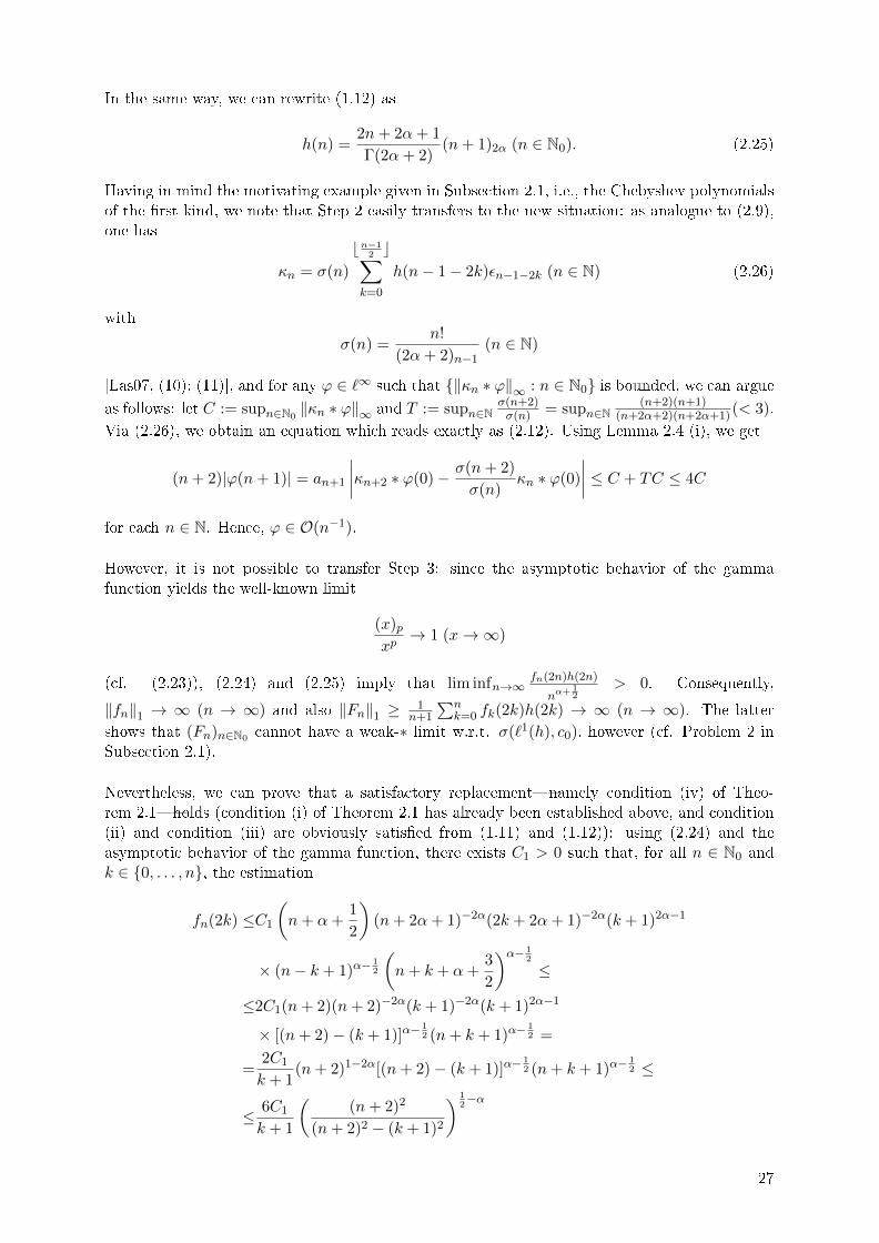
In the same way, we can rewrite (1.12) as

h(n) =2n+ 2α+ 1

Γ(2α+ 2)(n+ 1)2α (n ∈ N0). (2.25)

Having in mind the motivating example given in Subsection 2.1, i.e., the Chebyshev polynomialsof the �rst kind, we note that Step 2 easily transfers to the new situation: as analogue to (2.9),one has

κn = σ(n)

bn−12 c∑

k=0

h(n− 1− 2k)εn−1−2k (n ∈ N) (2.26)

with

σ(n) =n!

(2α+ 2)n−1(n ∈ N)

[Las07, (10); (11)], and for any ϕ ∈ `∞ such that {‖κn ∗ ϕ‖∞ : n ∈ N0} is bounded, we can argue

as follows: let C := supn∈N0‖κn ∗ ϕ‖∞ and T := supn∈N

σ(n+2)σ(n) = supn∈N

(n+2)(n+1)(n+2α+2)(n+2α+1)(< 3).

Via (2.26), we obtain an equation which reads exactly as (2.12). Using Lemma 2.4 (i), we get

(n+ 2)|ϕ(n+ 1)| = an+1

∣∣∣∣κn+2 ∗ ϕ(0)− σ(n+ 2)

σ(n)κn ∗ ϕ(0)

∣∣∣∣ ≤ C + TC ≤ 4C

for each n ∈ N. Hence, ϕ ∈ O(n−1).

However, it is not possible to transfer Step 3: since the asymptotic behavior of the gammafunction yields the well-known limit

(x)pxp→ 1 (x→∞)

(cf. (2.23)), (2.24) and (2.25) imply that lim infn→∞fn(2n)h(2n)

nα+12

> 0. Consequently,

‖fn‖1 → ∞ (n → ∞) and also ‖Fn‖1 ≥1

n+1

∑nk=0 fk(2k)h(2k) → ∞ (n → ∞). The latter

shows that (Fn)n∈N0 cannot have a weak-∗ limit w.r.t. σ(`1(h), c0), however (cf. Problem 2 inSubsection 2.1).

Nevertheless, we can prove that a satisfactory replacement�namely condition (iv) of Theo-rem 2.1�holds (condition (i) of Theorem 2.1 has already been established above, and condition(ii) and condition (iii) are obviously satis�ed from (1.11) and (1.12)): using (2.24) and theasymptotic behavior of the gamma function, there exists C1 > 0 such that, for all n ∈ N0 andk ∈ {0, . . . , n}, the estimation

fn(2k) ≤C1

(n+ α+

1

2

)(n+ 2α+ 1)−2α(2k + 2α+ 1)−2α(k + 1)2α−1

× (n− k + 1)α−12

(n+ k + α+

3

2

)α− 12

≤

≤2C1(n+ 2)(n+ 2)−2α(k + 1)−2α(k + 1)2α−1

× [(n+ 2)− (k + 1)]α−12 (n+ k + 1)α−

12 =

=2C1

k + 1(n+ 2)1−2α[(n+ 2)− (k + 1)]α−

12 (n+ k + 1)α−

12 ≤

≤ 6C1

k + 1

((n+ 2)2

(n+ 2)2 − (k + 1)2

) 12−α

27

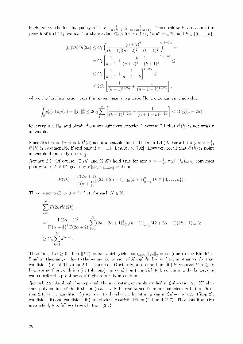
holds, where the last inequality relies on 1n+k+1 ≤

3(n+2)+(k+1) . Thus, taking into account the

growth of h (1.14), we see that there exists C2 > 0 such that, for all n ∈ N0 and k ∈ {0, . . . , n},

fn(2k)2h(2k) ≤ C2

((n+ 2)2

(k + 1)[(n+ 2)2 − (k + 1)2]

)1−2α

=

= C2

[1

k + 1+

k + 1

(n+ 2)2 − (k + 1)2

]1−2α

≤

≤ C2

[1

k + 1+

1

n+ 1− k

]1−2α

≤

≤ 2C2

[1

(k + 1)1−2α+

1

(n+ 1− k)1−2α

],

where the last estimation uses the power mean inequality. Hence, we can conclude that∫Rp4n(x) dµ(x) = ‖fn‖22 ≤ 2C2

n∑k=0

[1

(k + 1)1−2α+

1

(n+ 1− k)1−2α

]< 4C2ζ(1− 2α)

for every n ∈ N0, and obtain from our su�cient criterion Theorem 2.1 that `1(h) is not weaklyamenable.

Since h(n)→∞ (n→∞), `1(h) is not amenable due to Theorem 1.4 (i). For arbitrary α > −12 ,

`1(h) is xα-amenable if and only if x = ±1 [Las09c, p. 792]. However, recall that `1(h) is pointamenable if and only if α < 1

2 .

Remark 2.1. Of course, (2.24) and (2.25) hold true for any α > −12 , and (fn)n∈N0 converges

pointwise to F ∈ `∞ given by F |N0\{0,2,...,2n} = 0 and

F (2k) =Γ(2α+ 1)

Γ(α+ 1

2

)2 (2k + 2α+ 1)−2α(k + 1)2α− 1

2

(k ∈ {0, . . . , n}).

There is some Cα > 0 such that, for each N ∈ N,

N∑k=1

F (2k)2h(2k) =

=Γ(2α+ 1)2

Γ(α+ 1

2

)4Γ(2α+ 2)

N∑k=1

(2k + 2α+ 1)2−2α(k + 1)4

α− 12

(4k + 2α+ 1)(2k + 1)2α ≥

≥ CαN∑k=1

k2α−1.

Therefore, if α ≥ 0, then ‖F‖22 = ∞, which yields supn∈N0‖fn‖2 = ∞ (due to the Eberlein�

Smulian theorem, or due to the sequential version of Alaoglu's theorem) or, in other words, thatcondition (iv) of Theorem 2.1 is violated. Obviously, also condition (iii) is violated if α ≥ 0;however neither condition (ii) (obvious) nor condition (i) is violated: concerning the latter, onecan transfer the proof for α < 0 given in this subsection.

Remark 2.2. As should be expected, the motivating example studied in Subsection 2.1 (Cheby-shev polynomials of the �rst kind) can easily be reobtained from our su�cient criterion Theo-rem 2.1: w.r.t. condition (i) we refer to the short calculation given in Subsection 2.1 (Step 2);condition (ii) and condition (iii) are obviously satis�ed from (2.4) and (2.7). That condition (iv)is satis�ed, too, follows trivially from (2.8).

28

3. Complete characterizations of point and weak amenability forspeci�c classes

Parts of Section 3 are very similar to our publication [Kah15].

In Section 2.5, we solved the problem of weak amenability for the class of ultraspherical polyno-mials. In the present section, we extend this result to important one-parameter generalizationsof the ultraspherical polynomials, namely to the classes of Jacobi, symmetric Pollaczek and as-sociated ultraspherical polynomials. We give complete characterizations of both point and weakamenability of the `1-algebras by specifying the corresponding parameter regions. In the fol-lowing, we recall some basics and refer to [Las83, Sections 3 (a), (b)] and [Las94, Sections 3,4].

� Given α, β > −1, the sequence (R(α,β)n (x))n∈N0 of Jacobi polynomials which corresponds

to α and β is determined by its orthogonalization measure

dµ(x) =Γ(α+ β + 2)

2α+β+1Γ(α+ 1)Γ(β + 1)(1− x)α(1 + x)βχ(−1,1)(x) dx

and the normalization R(α,β)n (1) = 1 (n ∈ N0), or, equivalently, via

a0 =2α+ 2

α+ β + 2, an =

(α+ β + 2)(n+ α+ 1)(n+ α+ β + 1)

(α+ 1)(2n+ α+ β + 1)(2n+ α+ β + 2)(n ∈ N),

cn =(α+ β + 2)n(n+ β)

(α+ 1)(2n+ α+ β)(2n+ α+ β + 1)(n ∈ N),

bn ≡ 1− an − cn.

(3.1)

The corresponding parameter region DP ⊆ (− 1,∞)2 such that property (P) holds if andonly if (α, β) ∈ DP is

DP =

{(α, β) ∈

[−1

2,∞)× (−1,∞) : α ≥ β, a(a+ 5)(a+ 3)2 ≥ (a2 − 7a− 24)b2

},

where a = α+ β + 1 and b = α− β [Gas70, Theorem 1]; one has h(0) = 1 and

h(n) =(2n+ α+ β + 1)(α+ β + 2)n−1(α+ 1)n

n!(β + 1)n(n ∈ N). (3.2)

The hypergeometric representation of the Jacobi polynomials reads

R(α,β)n (x) = 2F1

(−n, n+ α+ β + 1

α+ 1

∣∣∣∣ 1− x2

)(n ∈ N0)

[KLS10, (9.8.1)].

� Given α > −12 , λ ≥ 0, the sequence (Q

(α,λ)n (x))n∈N0 of symmetric Pollaczek polynomials

which corresponds to α and λ is determined by its orthogonalization measure

dµ(x) = Cα,λ(1− x2)αeλx(2 arccos x−π)√

1−x2

∣∣∣∣Γ(α+1

2+

iλx√1− x2

)∣∣∣∣2 χ(−1,1)(x) dx, (3.3)

where Cα,λ > 0 is a constant such that µ has total mass 1, and the normalization

Q(α,λ)n (1) = 1 (n ∈ N0). Equivalently, (Q

(α,λ)n (x))n∈N0 is given via

bn ≡ 0, an ≡ 1− bn − cn, cn :=n

2n+ 2α+ 2λ+ 1

∑n−1k=0

(n−1k

) (2λ)k

(2α+1)k∑nk=0

(nk

) (2λ)k

(2α+1)k

(n ∈ N).

29

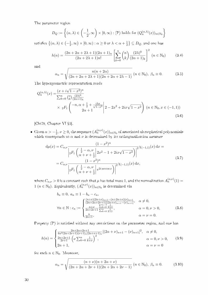
The parameter region

DQ :=

{(α, λ) ∈

(−1

2,∞)× [0,∞) : (P) holds for (Q(α,λ)

n (x))n∈N0

}satis�es

{(α, λ) ∈

(−1

2 ,∞)× [0,∞) : α ≥ 0 or λ < α+ 1

2

}⊆ DQ, and one has

h(n) =(2n+ 2α+ 2λ+ 1)(2α+ 1)n

(2α+ 2λ+ 1)n!

[n∑k=0

(n

k

)(2λ)k

(2α+ 1)k

]2

(n ∈ N0) (3.4)

and

αn =

√n(n+ 2α)

(2n+ 2α+ 2λ+ 1)(2n+ 2α+ 2λ− 1)(n ∈ N0), βn ≡ 0. (3.5)

The hypergeometric representation reads

Q(α,λ)n (x) =

(x+ i√

1− x2)n∑nk=0

(nk

) (2λ)k

(2α+1)k

× 2F1

(−n, α+ 1

2 + iλx√1−x2

2α+ 1

∣∣∣∣∣ 2− 2x2 + 2ix√

1− x2

)(n ∈ N0, x ∈ (−1, 1))

(3.6)

[Chi78, Chapter VI �5].

� Given α > −12 , ν ≥ 0, the sequence (A

(α,ν)n (x))n∈N0 of associated ultraspherical polynomials

which corresponds to α and ν is determined by its orthogonalization measure

dµ(x) = Cα,ν(1− x2)α∣∣∣∣2F1

(12 − α, να+ ν + 1

2

∣∣∣∣ 2x2 − 1 + 2ix√

1− x2

)∣∣∣∣2χ(−1,1)(x) dx =

= Cα,ν(1− x2)α∣∣∣∣2F1

(12 − α, να+ ν + 1

2

∣∣∣∣ e2i arccosx

)∣∣∣∣2χ(−1,1)(x) dx,

(3.7)

where Cα,ν > 0 is a constant such that µ has total mass 1, and the normalization A(α,ν)n (1) =

1 (n ∈ N0). Equivalently, (A(α,ν)n (x))n∈N0 is determined via

bn ≡ 0, an ≡ 1− bn − cn,

∀n ∈ N : cn :=

(n+ν)(2α+ν)n+1−(n+2α+ν)(ν)n+1

(2n+2α+2ν+1)[(2α+ν)n+1−(ν)n+1] , α 6= 0,

n+ν2n+2ν+1

∑n−1k=0

1k+ν∑n

k=01

k+ν

, α = 0, ν > 0,

n2n+1 , α = ν = 0.

(3.8)

Property (P) is satis�ed without any restrictions on the parameter region, and one has

h(n) =

2n+2α+2ν+1

4α2(2α+2ν+1)(ν+1)n(2α+ν+1)n[(2α+ ν)n+1 − (ν)n+1]2, α 6= 0,

2n+2ν+12ν+1

(ν∑n

k=01

k+ν

)2, α = 0, ν > 0,

2n+ 1, α = ν = 0

(3.9)

for each n ∈ N0. Moreover,

αn =

√(n+ ν)(n+ 2α+ ν)

(2n+ 2α+ 2ν + 1)(2n+ 2α+ 2ν − 1)(n ∈ N0), βn ≡ 0. (3.10)

30

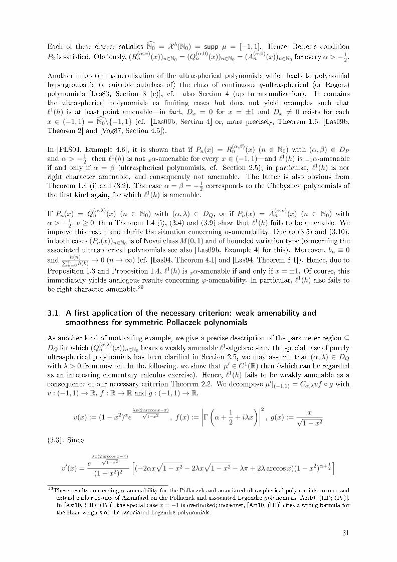
Each of these classes satis�es N0 = X b(N0) = supp µ = [−1, 1]. Hence, Reiter's condition

P2 is satis�ed. Obviously, (R(α,α)n (x))n∈N0 = (Q

(α,0)n (x))n∈N0 = (A

(α,0)n (x))n∈N0 for every α > −1

2 .

Another important generalization of the ultraspherical polynomials which leads to polynomialhypergroups is (a suitable subclass of) the class of continuous q-ultraspherical (or Rogers)polynomials [Las83, Section 3 (c)], cf. also Section 4 (up to normalization). It containsthe ultraspherical polynomials as limiting cases but does not yield examples such that`1(h) is at least point amenable�in fact, Dx = 0 for x = ±1 and Dx 6= 0 exists for eachx ∈ (−1, 1) = N0\{−1, 1} (cf. [Las09b, Section 4] or, more precisely, Theorem 1.6, [Las09b,Theorem 2] and [Vog87, Section 4.5]).

In [FLS04, Example 4.6], it is shown that if Pn(x) = R(α,β)n (x) (n ∈ N0) with (α, β) ∈ DP

and α > −12 , then `

1(h) is not xα-amenable for every x ∈ (−1, 1)�and `1(h) is −1α-amenableif and only if α = β (ultraspherical polynomials, cf. Section 2.5); in particular, `1(h) is notright character amenable, and consequently not amenable. The latter is also obvious fromTheorem 1.4 (i) and (3.2). The case α = β = −1

2 corresponds to the Chebyshev polynomials ofthe �rst kind again, for which `1(h) is amenable.

If Pn(x) = Q(α,λ)n (x) (n ∈ N0) with (α, λ) ∈ DQ, or if Pn(x) = A

(α,ν)n (x) (n ∈ N0) with

α > −12 , ν ≥ 0, then Theorem 1.4 (i), (3.4) and (3.9) show that `1(h) fails to be amenable. We

improve this result and clarify the situation concerning α-amenability. Due to (3.5) and (3.10),in both cases (Pn(x))n∈N0 is of Nevai classM(0, 1) and of bounded variation type (concerning theassociated ultraspherical polynomials see also [Las09b, Example 4] for this). Moreover, bn ≡ 0

and h(n)∑nk=0 h(k)

→ 0 (n→∞) (cf. [Las94, Theorem 4.1] and [Las94, Theorem 3.1]). Hence, due to

Proposition 1.3 and Proposition 1.4, `1(h) is xα-amenable if and only if x = ±1. Of course, thisimmediately yields analogous results concerning ϕ-amenability. In particular, `1(h) also fails tobe right character amenable.29

3.1. A �rst application of the necessary criterion: weak amenability andsmoothness for symmetric Pollaczek polynomials

As another kind of motivating example, we give a precise description of the parameter region ⊆DQ for which (Q

(α,λ)n (x))n∈N0 bears a weakly amenable `1-algebra; since the special case of purely

ultraspherical polynomials has been clari�ed in Section 2.5, we may assume that (α, λ) ∈ DQ

with λ > 0 from now on. In the following, we show that µ′ ∈ C1(R) then (which can be regardedas an interesting elementary calculus exercise). Hence, `1(h) fails to be weakly amenable as aconsequence of our necessary criterion Theorem 2.2. We decompose µ′|(−1,1) = Cα,λvf ◦ g withv : (−1, 1)→ R, f : R→ R and g : (−1, 1)→ R,

v(x) := (1− x2)αeλx(2 arccos x−π)√

1−x2 , f(x) :=

∣∣∣∣Γ(α+1

2+ iλx

)∣∣∣∣2 , g(x) :=x√

1− x2

(3.3). Since

v′(x) =eλx(2 arccos x−π)√

1−x2

(1− x2)2

[(−2αx

√1− x2 − 2λx

√1− x2 − λπ + 2λ arccosx)(1− x2)α+ 1

2

]29These results concerning α-amenability for the Pollaczek and associated ultraspherical polynomials correct and

extend earlier results of Azimifard on the Pollaczek and associated Legendre polynomials [Azi10, (III); (IV)].In [Azi10, (III); (IV)], the special case x = −1 is overlooked; moreover, [Azi10, (III)] cites a wrong formula forthe Haar weights of the associated Legendre polynomials.

31

for x ∈ (−1, 1), we see that

|v′(x)| ≤ eλx(2 arccos x−π)√

1−x2

(1− x2)2≤ e

− λ√1−x2

(1− x2)2

if 1−|x| is su�ciently small. Consequently, v ∈ C1(−1, 1) and limx→±1 v′(x) = 0 = limx→±1 v(x).

We now study the function f . Euler's in�nite product formula for the complex gamma functionstates that

Γ(z) =1

z

∞∏n=1

(1 + 1

n

)z1 + z

n

(z ∈ C,−z /∈ N0)

[GK97, Proposition 15.1.6], and it is a consequence of this that

|Γ(x+ iy)|2 = Γ(x)2∞∏n=0

(x+ n)2

(x+ n)2 + y2(x, y ∈ R,−(x+ iy) /∈ N0) (3.11)

[AS64, 6.1.25]. From (3.11) we obtain that

log f(x) = 2 log Γ

(α+

1

2

)+∞∑n=0

log

(α+ 1

2 + n)2(

α+ 12 + n

)2+ λ2x2︸ ︷︷ ︸

=:γn(x)

(x ∈ R).

Since γn : R→ R, x 7→ γn(x), is continuously di�erentiable for each n ∈ N0 with

γ′n(x) =−2λ2x(

α+ 12 + n

)2+ λ2x2

(x ∈ R),

and since the series∑∞

n=0 γ′n(x) converges uniformly on compact intervals, we see that log f ∈

C1(R) andd

dxlog f(x) = −2λ2x

∞∑n=0

1(α+ 1

2 + n)2

+ λ2x2(x ∈ R).

Consequently, f ∈ C1(R) with

f ′(x) = −2λ2xf(x)

∞∑n=0

1(α+ 1

2 + n)2

+ λ2x2(x ∈ R).

In particular, we have established the existence of a constant C1 > 0 such that |f ′(x)| ≤C1|x|f(x) (x ∈ R) and hence obtain

|(f ◦ g)′(x)| ≤ C1|g(x)|f ◦ g(x)|g′(x)| = C1|x|

(1− x2)2f ◦ g(x) (x ∈ (−1, 1)). (3.12)

As a consequence of (a well-known variant of) Stirling's formula [AAR99, Corollary 1.4.4], thereis a constant C2 > 0 such that

|f ◦ g(x)| ≤ C2|g(x)|2αe−λπ|g(x)| (x ∈ (−1, 1));

in view of (3.12), this yields a constant C3 > 0 such that

|(f ◦ g)′(x)| ≤ C3|g(x)|2α+4e−λπ|g(x)|

if x ∈ (−1, 1) is such that 1− |x| is su�ciently small. So we can conclude that f ◦ g ∈ C1(−1, 1)and limx→±1(f ◦ g)′(x) = 0 = limx→±1 f ◦ g(x); putting all together, we see that indeedµ′ ∈ C1(R), and that, due to Theorem 2.2, {‖κn‖∞ : n ∈ N0} is bounded and `1(h) fails to beweakly amenable.

In Subsection 3.3, we shall see that `1(h) even fails to be point amenable whenever λ > 0�witha considerably more involved argument, however.

32

3.2. Jacobi polynomials: transition from the purely ultraspherical case, and howto avoid dealing with a 9F8

Our main result on Jacobi polynomials is the following theorem, which corresponds to [Kah15,Theorem 3.1] and gives complete characterizations concerning point and weak amenability.

Theorem 3.1. Let (α, β) ∈ DP , and let Pn(x) = R(α,β)n (x) (n ∈ N0). Then `1(h) is

(i) point amenable if and only if α < 12 (where Dx 6= 0 exists for each x ∈ (−1, 1) if α ≥ 1

2and D−1 6= 0 exists if and only if α ≥ β + 2),

(ii) weakly amenable if and only if α < 0.

Our proof of Theorem 3.1 relies on four lemmas, and we use the following notation:

∆ := {(α, β) ∈ DP : α+ β + 1 ≥ 0}

and

φn := R(α,β)n (−1) = (−1)n

(β + 1)n(α+ 1)n

(n ∈ N0).

Of course, φn depends on α, β > −1. The explicit formula for φn follows from the second equationin [Ism09, (4.1.6)] (note that our normalization does not coincide with that used in [Ism09], cf.the �rst equation in [Ism09, (4.1.6)]). The asymptotics of the gamma function yield

φn = Θ(nβ−α) (n→∞). (3.13)

The �rst lemma [Kah15, Lemma 3.1] gives an explicit formula for the sequence (κn)n∈N andgeneralizes (2.9) and (2.26).

Lemma 3.1. If (α, β) ∈ DP and Pn(x) = R(α,β)n (x) (n ∈ N0), then

κn(k) = σ(n)φn − φkφn − φn−1

(n ∈ N, k ∈ {0, . . . , n}). (3.14)

Concerning asymptotic behavior, we obtain from (3.2), Lemma 2.4 (i), Lemma 3.1 and (3.13):

h(n) = Θ(n2α+1), σ(n) = Θ(n−2α), τ(n) =

{Θ(n−α−β), α 6= β,

O(n−2α), α = β(3.15)

as n→∞.

In Section 2.5, we saw that Step 2 of Section 2.1 easily transfers from the Chebyshev polyno-mials of the �rst kind to arbitrary ultraspherical polynomials. It is considerably more involved(and the most technical part of Theorem 3.1) to obtain an analogue for non-symmetric Jacobipolynomials�i.e., to verify condition (i) of Theorem 2.1 (as far as a veri�cation is necessary forour proof of Theorem 3.1; in fact, we shall see that it is not necessary to deal with the whole set{(α, β) ∈ DP : α < 0} but it su�ces to consider a proper subset and, after a successful applica-tion of Theorem 2.1 to this subset, to use inheritance via homomorphisms). Our second lemma[Kah15, Lemma 3.2] provides an auxiliary function which will become a crucial tool concerningthe just outlined strategy.

Lemma 3.2. If (α, β) ∈ DP , α 6= β, and Pn(x) = R(α,β)n (x) (n ∈ N0), then the function

η : N→ [0,∞),

η(n) :=n+ 2

h(n+ 1)

n∑k=0

h(k)

k + 1

∣∣∣∣ κn+2(k)

σ(n+ 2)− κn(k)τ(n+ 2)

τ(n)σ(n+ 2)

∣∣∣∣ ,is well-de�ned and satis�es limn→∞ η(n) = α−β

2α+1 .

33

Concerning condition (iv) of Theorem 2.1, we have the following [Kah15, Lemma 3.3]:

Lemma 3.3. If (α, β) ∈ DP , α < 0, and Pn(x) = R(α,β)n (x) (n ∈ N0), then

supn∈N0

∫Rp

4n(x) dµ(x) <∞.

Finally, the fourth lemma [Kah15, Lemma 3.4] is helpful w.r.t. inheritance via homomorphisms�more precisely, w.r.t. applications of Theorem 2.3 and Proposition 2.2.

Lemma 3.4. Let (α, β), (γ, δ) ∈ DP , and let for each n ∈ N0 the connec-tion coe�cients CPn (α, β; γ, δ)(0), . . . , CPn (α, β; γ, δ)(n) be de�ned by R

(α,β)n (x) =∑n

k=0CPn (α, β; γ, δ)(k)R

(γ,δ)k (x). Then each of the following conditions is su�cient for

the existence of some C > 0 such that∑n

k=0 |CPn (α, β; γ, δ)(k)| ≤ C (n ∈ N0): (A) γ ≤ α andδ = β, (B) γ = α and δ ≥ β, (C) γ = α− ξ and δ = β − ξ for some ξ ≥ 0.

Lemma 3.1 can be established very quickly via the Jacobi forward shift

d

dxR(α,β)n (x) =

n(n+ α+ β + 1)

2α+ 2R

(α+1,β+1)n−1 (x) (n ∈ N) (3.16)

[Ism09, (4.1.6); (4.2.2)],30 the connection coe�cients w.r.t. the original sequence [Ism09, Section9.1] (cf. also [Doh02]) and several ingredients from the theory of hypergeometric series (certaincontiguous relations, Chu�Vandermonde identity [AAR99, Corollary 2.2.3], Pfa��Saalschützidentity [AAR99, Theorem 2.2.6]). This way is presented in our paper [Kah15]. A very similarargument is used in [IS12]. Another direct proof is contained in the author's Master's thesis andbased on kernel polynomials [Kah12, Section 3.4.2]. Alternatively, one could also use inductionand a general recurrence relation for the sequence (κn)n∈N0 , cf. [Las07, (5)] and Remark 1.1,and cf. also (4.12) and (4.21) in Section 4 (which studies a di�erent setting, however). This wasdone by E. Perreiter (independently of the author). Lemma 3.2 is a consequence of Lemma 3.1and the Stolz�Cesàro theorem. Lemma 3.3 relies on ideas from [Sze75, Chapter 7.34] andsuitable asymptotics of the Jacobi polynomials (which follow from [Sze75, Chapter 7.32] andare consequences of a formula of Mehler�Heine type and a formula of Darboux, or also of aformula of Hilb's type). If β ≥ −1

2 , the polynomials p4n(x) (n ∈ N0) even have a µ-integrable

majorant on (−1, 1)�namely the function R → [0,∞), x 7→ C(1−x)2α+1(1+x)2β+1χ(−1,1)(x), with

C ∈ R independent of x. This is a consequence of [NEM94, Theorem 1] (which, however, is fornon-symmetric Jacobi polynomials a rather deep result that has led to the Erdélyi�Magnus�Nevai conjecture which deals with the occurring constants C). Lemma 3.4 follows from resultsof [Bav71]. (B) and its proof via [Bav71] are already contained in E. Perreiter's dissertation[Per11a, Corollary 3.12].

Trying to prove Lemma 3.3 in a way which directly imitates the strategy presented in Section 2.5for the purely ultraspherical case, i.e., transforming∫

Rp4n(x) dµ(x) =

2n∑k=0

[g(n, k;n)]2h(k) (n ∈ N0)

via (2.3) and estimating the right hand sides from above by using explicit formulas for thelinearization coe�cients g(m,n; k), would be a �rather bad idea�: for non-symmetric (and�non-special�) Jacobi polynomials, these formulas are much more complicated than Dougall'sformula (2.22)�Rahman's formula, for instance, which works (and explicitly shows property

30In contrast to (3.16), the Jacobi backward shift reads

(1− x2)d

dxR(α+1,β+1)n (x) = (2α+ 2)

[R

(α,β)1 (x)R(α+1,β+1)

n (x)−R(α,β)n+1 (x)

](n ∈ N0), (3.17)

cf. [Ism09, (4.1.6); (4.2.5)] and (3.1). We shall refer to this later.

34

(P)) for the pairs (α, β) ∈ ∆, involves a 9F8 hypergeometric series [Rah81].

In view of earlier results (cf. [Las09b, Section 4]), concerning Theorem 3.1 (i) it is just left to usto establish point amenability for (α, β) ∈ DP \∆. Of course, this will follow from Theorem 3.1(ii). More directly, it can be obtained from Proposition 2.2 and Lemma 3.4: if (α, β) ∈ DP \∆,then (α+ ξ, β) ∈ ∆ for some ξ ∈

(0,−α+ 1

2

).

The failure of weak amenability for α ≥ 0 was shown in E. Perreiter's dissertation [Per11a,Corollary 3.12]; the proof corresponds to an application of Theorem 2.3 (inheritance viahomomorphisms), Lemma 3.4 (B) and the failure of weak amenability for the ultrasphericalpolynomials corresponding to α.

The di�cult part concerning the proof of Theorem 3.1 (ii) is to establish weak amenability forα < 0. In view of Theorem 2.3 and Lemma 3.4, we may additionally assume that (α, β) is locatedin the interior of ∆. In this situation, the conditions of our su�ciency criterion Theorem 2.1can be seen to be satis�ed: (ii) and (iii) are clear, (iv) is a consequence of Lemma 3.3, and ourproof of the remaining condition (i) can be outlined as follows:

let ϕ ∈ `∞ such that {‖κn ∗ ϕ‖∞ : n ∈ N0} is bounded, let C := supn∈N0‖κn ∗ ϕ‖∞, let η be

as in Lemma 3.2, let S := limn→∞ η(n) < 1 (the latter is a consequence of Lemma 3.2), let

T := supn∈N

∣∣∣ τ(n+2)τ(n)

∣∣∣ <∞ (this follows from (3.15); with regard to well-de�nedness of quotients

containing τ(n), note that we have τ(n) 6= 0 (n ∈ N) because α 6= β), let N ∈ N such that

η(n) ≤ S+12 for all n ∈ N with n ≥ N , and, �nally, let M := max

((N + 1) ‖ϕ‖∞ ,

4+4T1−S C

).

Then use induction on n to show that

|ϕ(n)| ≤ M

n+ 1

for each n ∈ N0. This is the tedious non-symmetric analogue to Step 2 in Section 2.1 (and tothe easier�still symmetric�generalization contained in Section 2.5). As in Section 2.1 and inSection 2.5, the details rely on a consideration of (κn ∗ ϕ(0))n∈N0 .

The detailed proofs of Theorem 3.1 and the four lemmas can be found in our paper [Kah15].

In contrast to Abelian locally compact groups, for arbitrary polynomial hypergroups there isno Pontryagin duality (despite their commutativity): in fact, the only polynomial hypergroupsfor which N0 is a hypergroup w.r.t. pointwise multiplication and complex conjugation (andwhich are also `Pontryagin' then [BH95, Proposition 2.4.18])�cf. [BH95, Chapter 2.4] for the

precise de�nitions and some properties�correspond to Jacobi polynomials (R(α,β)n (x))n∈N0 with

(α, β) ∈ DP such that either β ≥ −12 or α + β ≥ 0 [CS90] [BH95, Section 3.6]. Combining this

with Theorem 3.1, we see that each of the cases �`1(h) amenable�, �`1(h) weakly amenable butnot right character amenable�, �`1(h) point amenable but neither right character amenable norweakly amenable� and �`1(h) not point amenable� can occur even in the class of Pontryaginpolynomial hypergroups.

Theorem 3.1 has also some interesting consequences w.r.t. our general results presented inSection 2:

� Theorem 2.2 tells that the boundedness of the set {‖κn‖∞ : n ∈ N0} is equivalent to theboundedness of the single function τ . However, as outlined in Section 2.3, this is in generalnot equivalent to the boundedness of σ (whose computation would be considerably easier,

see Lemma 2.4 (i)): if, for example, Pn(x) = R(α,β)n (x) (n ∈ N0) with α > 0, β > −1 and

α+ β < 0, then τ(n)→∞ (n→∞) but σ(n)→ 0 (n→∞). This follows from (3.15).

35

� (i) of our necessity criterion Theorem 2.2, i.e., the unboundedness of τ , is not su�cient forweak amenability of `1(h). We can take the examples of the previous item to see this. Inparticular, (ii) of Theorem 2.2, i.e., that µ is not absolutely continuous (as a measure) or µ′

is not absolutely continuous on the convex hull of supp µ (as a function), is not su�cient forweak amenability. Recall that the conditions of our su�ciency criterion Theorem 2.1 canbe regarded as a suitable sharpening of (ii) of Theorem 2.2 (and also of (i) of Theorem 2.2);cf. the note at the end of Section 2.3.

� If α and β are chosen from the smaller region α ≥ 12 , β > −1, α + β < 0, and if still

Pn(x) = R(α,β)n (x) (n ∈ N0), then `1(h) is not even point amenable (in fact, there exist

nonzero bounded point derivations at every x ∈ (−1, 1)). Thus condition (i) (and hencecondition (ii)) of Theorem 2.2 is also not su�cient for point amenability of `1(h).

� Finally, (ii) (and therefore (i)) of Theorem 2.2 is not necessary for point amenability of

`1(h): if 0 ≤ α < 12 and Pn(x) = P

(α)n (x) (n ∈ N0), then `1(h) is point amenable (already

due to [Las09b, Corollary 1]), but (ii) of Theorem 2.2 is not satis�ed. The same examplesshow that neither condition (iii) nor condition (iv) of Theorem 2.1 is necessary for pointamenability of `1(h) (cf. the notes at the end of Section 2.5, in part. Remark 2.1). The littleq-Legendre polynomials provide examples which show that condition (ii) of Theorem 2.1is not necessary for point amenability of `1(h) (cf. the notes at the end of Section 2.3).

� With regard to the comment at the end of Section 2.3, we note that if (ii) of Theorem 2.2is satis�ed, then h can nevertheless be of superlinear growth (see the examples above).

3.3. Symmetric Pollaczek polynomials: transformations and estimations of thederivatives

In the motivating Subsection 3.1, we used Theorem 2.2 to rule out weak amenability for allPollaczek polynomials (Q

(α,λ)n (x))n∈N0 with (α, λ) ∈ DQ, λ > 0. As announced in Subsection 3.1,

we now sharpen this result and show that even point amenability fails in this situation. Thefollowing is [Kah15, Theorem 4.1].

Theorem 3.2. Let (α, λ) ∈ DQ and Pn(x) = Q(α,λ)n (x) (n ∈ N0). Then `1(h) is

(i) point amenable if and only if α < 12 and λ = 0,

(ii) weakly amenable if and only if α < 0 and λ = 0.

(ii) is completely contained in the earlier parts of this thesis. Concerning the proof of (i), wedistinguish three cases: the case α < 1

2 and λ = 0 corresponds just to point amenability of

ultraspherical polynomials [Las09b, Corollary 1]. The case α+ λ ≥√

8α+52 − 1 can be solved by

extending an argument which has been given in [Las09b, Example 7] for (the subcase) α+λ ≥ 1.This argument corresponds to our Proposition 2.1 (i).

The remaining case 0 < λ < −α+√

8α+52 − 1 is much more interesting and the actual di�culty

in the proof of Theorem 3.2 (i): neither (i) nor (ii) of Proposition 2.1 applies;31 our strategywill be quite di�erent and can be outlined as the following idea: �rst transform the Pollaczekpolynomials into a system of orthogonal polynomials which is closely related yet more convenient(particularly with regard to asymptotic behavior)�then, based on this transformation, showthat the derivatives of the Pollaczek polynomials are bounded at 0, which yields a nonzerobounded point derivation due to Theorem 1.6.

31A very fast yet not trivial way to see that limn→∞ cn = 12(in the whole class of symmetric Pollaczek polynomials)

would be to apply a relationship to the Laguerre polynomials [Las94, Section 4] and Perron's formula in thecomplex plane [Sze75, Theorem 8.22.3].

36

The more convenient class we have in mind is the class of random walk polynomials32, cf. [Las83,Section 3 (d)] [Las94, Sections 6, 7] in the following: given a ≥ 1 and b ≥ 0, the sequence

(S(a,b)n (x))n∈N0 of random walk polynomials which corresponds to a and b is determined by its

orthogonalization measure

dµ(x) = Ca,b[4a− (a+ 1)2x2]b2a− 1

2 exp

(a− 1)bx[2 arccos

(a+12√ax)− π

]2a√

4a− (a+ 1)2x2

×

∣∣∣∣∣Γ(b

2a+

i(a− 1)bx

2a√

4a− (a+ 1)2x2

)∣∣∣∣∣2

χ(− 2√a

a+1, 2√a

a+1

)(x) dx

if b > 0 and

dµ(x) = Ca,0

√4a− (a+ 1)2x2

1− x2χ(− 2

√a

a+1, 2√a

a+1

)(x) dx

if b = 0, with suitable Ca,b, Ca,0 > 0,33 and the normalization S(a,b)n (1) = 1 (n ∈ N0)�or,

equivalently, but in a much simpler form, via

bn ≡ 0, an ≡ 1− bn − cn, cn :=n

(a+ 1)n+ b(n ∈ N). (3.18)

Obviously,

S(1,b)n (x) = P

( b−12 )

n (x) (b ≥ 0, n ∈ N0). (3.19)

Property (P) holds for all a ≥ 1 and b ≥ 0, and one has N0 = [−1, 1] and

X b(N0) =

{z ∈ C :

∣∣∣∣z − 2√a

a+ 1

∣∣∣∣+

∣∣∣∣z +2√a

a+ 1

∣∣∣∣ ≤ 2

}.

The Haar weights satisfy h(0) = 1 and

h(n) =

{an( ba)

n[(a+1)n+b]

bn! , b > 0,

(a+ 1)an−1, b = 0(3.20)

for n ∈ N. The relationship to the Pollaczek polynomials reads as follows:

S(a,b)n (x) =

Q( b2a− 1

2,b( 1

a+1− 1

2a))n

(a+12√ax)

Q( b2a− 1

2,b( 1

a+1− 1

2a))n

(a+12√a

) (n ∈ N0) (3.21)

and

Q(α,λ)n (x) =

S( 2α+2λ+12α−2λ+1

,(2α+1) 2α+2λ+12α−2λ+1)

n

(√1−

(2λ

2α+1

)2x

)

S( 2α+2λ+12α−2λ+1

,(2α+1) 2α+2λ+12α−2λ+1)

n

(√1−

(2λ

2α+1

)2) (n ∈ N0), (3.22)

provided a ≥ 1, b > 0 in (3.21), and α > −12 , 0 ≤ λ < α + 1

2 in (3.22) (the denominators arenonzero).

The following lemma [Kah15, Lemma 4.1] is our central auxiliary tool:

32Concerning the relation to random walks, we refer to [AI84, Section 6]. To avoid confusions, we note thatin Section 4 we will use the expression �random walk polynomials� in a rather di�erent, much more generalmanner.

33We note that the case b > 0 is stated with a typo in [Las94, Section 7]. That our formula is the correct one canbe seen from the proof of [Las94, Theorem (7.1)]; cf. also [AI84, Section 6].

37

Lemma 3.5. Let α > −12 , 0 ≤ λ < α+ 1

2 . Let

ρ :=

√1−

(2λ

2α+ 1

)2

, γ :=

√2α− 2λ+ 1

2α+ 2λ+ 1,

and let

sn :=(2α+ 2λ+ 1)(n+ 2α+ 1)

(2α+ 1)(2n+ 2α+ 2λ+ 1), tn := 1− sn =

(2α− 2λ+ 1)n

(2α+ 1)(2n+ 2α+ 2λ+ 1)(n ∈ N).

Then the recurrence relation ψ1 := ρ,

ψn+1 :=ρψn − tnsnψn

(n ∈ N),

de�nes a sequence (ψn)n∈N ⊆ [γ,∞) which satis�es

ψn ≥2λn+ 2α+ 1

2λn+ 2α− 2λ+ 1γ

for each n ∈ N.

Its elementary proof can be found in our paper [Kah15]. Based on Lemma 3.5, the proof of the

remaining case 0 < λ < −α +√

8α+52 − 1 (Theorem 3.2 (i)) can be sketched as follows: since

λ < α+ 12 , we can set Sn(x) := S

(a,b)n (x) with a := 2α+2λ+1

2α−2λ+1 > 1 and b := (2α + 1)2α+2λ+12α−2λ+1 > 0.

In the following, we use the notation of Lemma 3.5. (3.22) yields

P ′n(0) = ρS′n(0)

Sn(ρ)(n ∈ N0),

and one has S0(x) = 1, S1(x) = x,

xSn(x) = snSn+1(x) + tnSn−1(x) (n ∈ N).

It can be seen from the latter recurrence relation that

S′n(0) = O(nγn) (n→∞). (3.23)

Furthermore, this recurrence relation implies that Sn(ρ) =∏nk=1 ψk (n ∈ N)�hence, as a conse-

quence of Lemma 3.5, we obtain

1

Sn(ρ)= O(n−1γ−n) (n→∞). (3.24)

Putting all together, we can conclude that {P ′n(0) : n ∈ N0} is bounded and apply Theorem 1.6as desired. The details are given in our paper [Kah15].

Remark 3.1. Concerning the case 0 < λ < −α+√

8α+52 − 1 (Theorem 3.2 (i)), we observe:

(i) Comparing the random walk polynomials to the symmetric Pollaczek polynomials, wecould bene�t from the random walk polynomials in a twofold way. On the one hand,their recurrence coe�cients are of considerably easier structure. On the other hand�andmore important, while limn→∞ cn = limn→∞ an for the whole class of symmetric Pollaczekpolynomials, the two limits are obviously di�erent for the non-ultraspherical random walkpolynomials: it was the latter property which enabled us to estimate (S′n(0))n∈N0 (cf.(3.23)).

38

(ii) With regard to the proof of (3.24), there is a variant which does not require to useLemma 3.5 (nevertheless, we still use the notation of the lemma): applying [AI84, Sec-tion 6, in part. (6.30)], we obtain

1

Sn(ρ)= Θ(nα+ 1

4γ−ne−√

8λn) (n→∞), (3.25)

which obviously yields (3.24). However, the proof of (3.25) via the cited ingredient is muchless elementary than the proof of our Lemma 3.5; [AI84, (6.30)] relies on a relationshipto the Laguerre polynomials and Perron's formula in the complex plane [Sze75, Theorem8.22.3].

The strategy presented in Subsection 3.1 to rule out weak amenability whenever λ > 0 andthe strategy presented in the current subsection to even rule out point amenability for thoseλ show that {‖κn‖∞ : n ∈ N0} and {P ′n(0) : n ∈ N0} are bounded�without the need ofexplicit computations of κn (n ∈ N0), or ‖κn‖∞ (n ∈ N0), and P ′n(0) (n ∈ N0). Such explicitcomputations seem to be out of reach for this example class (which, concerning κn (n ∈ N0),contrasts with the Jacobi polynomials studied in Subsection 3.2): this shows the worth of the(general) necessity result Theorem 2.2 and the worth of the (concrete) transformation into therandom walk polynomials combined with the asymptotic approach. In particular, we think thattrying to estimate P ′n(0) (n ∈ N0) via (3.6) (or via similar hypergeometric representations forthe random walk polynomials, cf. [AI84, Section 6]) would not be a better idea.

As a consequence of Theorem 3.2, we see that even the combination of bn ≡ 0, the existence ofan n ∈ N with cnan−1 >

14 and the condition lim supn→∞ cn ≥ 1

2 (cf. Proposition 2.1) is notsu�cient for point amenability.

Point and weak amenability for the random walk polynomials themselves will be characterizedin Subsection 3.5.

3.4. Associated ultraspherical polynomials: interplay between hypergeometricand absolutely continuous Fourier series

Concerning the class of associated ultraspherical polynomials, point and weak amenability canbe characterized as follows [Kah15, Theorem 5.1]:

Theorem 3.3. Let α > −12 , ν ≥ 0, and Pn(x) = A

(α,ν)n (x) (n ∈ N0). Then `1(h) is

(i) point amenable if and only if α < 12 (where Dx 6= 0 exists for each x ∈ (−1, 1) if α ≥ 1

2 butD−1 = 0 always),

(ii) weakly amenable if and only if α < 0 and ν = 0.

The �if� part of (i) is shown in [Las09b, Example 4].34 The �only if� part, as well as the strongerassertion stated in the brackets, can be seen via Proposition 2.1 (i); this is motivated by [Ask71,Section 3].35 Taking into account (i) and the earlier results of this thesis, it remains to ruleout weak amenability for the parameter region α < 1

2 , ν > 0. The subcase α ≥ 0 is not verydi�cult and can be tackled by an homomorphism inheritance argument�more precisely, via thenonnegativity of the connection coe�cients to the ultraspherical polynomials {P (α)

n (x) : n ∈ N0}34We note that the reference contains a small mistake: in general, we do not have h(n) = O(n2α+1) (n→∞) as

stated in [Las09b, Example 4], but h(n) = O(n2|α|+1) if α 6= 0 and h(n) = O(nγ) for every γ > 1 if α = 0, cf.(3.9). One does not have h(n) = O(n) in the latter case (except if ν = 0). This mistake does not a�ect theconclusion, however.

35To avoid possible confusions, we note that the parametrization in [Ask71, Section 3] is slightly di�erent fromours: the parameter µ in [Ask71, Section 3] corresponds to our parameter ν, whereas ν in the referencecorresponds to α+ 1

2in our notation.

39

(see [Ask71, Section 3]) and Theorem 2.3; the special case α = 0 has already been solved in[LP10, Corollary 3.4] by using this method.

The subcase α < 0 is the actual di�culty in the proof of Theorem 3.3 (ii)�here, the connection

coe�cients to {P (α)n (x) : n ∈ N0} are still nonnegative [Ask71, Section 3], but the `1-algebra

which corresponds to these ultraspherical polynomials is, as we already have seen, weaklyamenable, and therefore the formerly successful homomorphism inheritance argument breaksdown. Instead, our strategy for α < 0 (which shall be assumed from now on) is basedon our necessity criterion Theorem 2.2. The strategy uses a similar decomposition of theRadon�Nikodym derivative (which shall turn out to be absolutely continuous on [−1, 1]) as inthe motivating Subsection 3.1; however, this is considerably more involved than ruling out weakamenability for the Pollaczek �counterparts� which were considered in Subsection 3.1. In thefollowing, we give a brief sketch.

Since the numerators in (3.7) have singularities at the boundary of supp µ, we �rst use Euler'stransformation formula for hypergeometric functions [AAR99, Theorem 2.2.5] to rewrite (3.7) as

dµ(x) = 16−αCα,ν(1− x2)−α∣∣∣∣2F1

(2α+ ν, α+ 1

2α+ ν + 1

2

∣∣∣∣ e2i arccosx

)∣∣∣∣2χ(−1,1)(x) dx. (3.26)

Now, at least the numerator is absolutely continuous on [−1, 1]. Concerning the denomina-

tor of (3.26) and well-de�nedness, we note that 2F1

(2α+ ν, α+ 1

2α+ ν + 1

2

∣∣∣∣ .) is absolutely convergent

[AAR99, Theorem 2.1.2] and nonzero [Run71] on the unit circle. Observe that the denominatorhas also a meaning with respect to Fourier series. We shall crucially bene�t from a fruitfulinterplay between hypergeometric and Fourier series, and we need the following auxiliary resulton absolute continuity [Kah15, Lemma 5.1]:

Lemma 3.6. Let (γn)n∈N0 ⊆ R such that∑∞

n=0 |γn| < ∞, and assume that there exists anN ∈ N0 such that 0 ≤ γn+1 ≤ n

n+1γn whenever n ≥ N . Then

(i) both functions Fc, Fs : [0, 2π] → R, Fc(x) :=∑∞

n=0 γn cos(nx), Fs(x) :=∑∞

n=1 γn sin(nx),are absolutely continuous,

(ii) the function G : [0, 2π]→ R, G(x) :=∣∣∑∞

n=0 γne−inx∣∣2, is absolutely continuous.

Our proof of Lemma 3.6 makes use of an idea presented in [Tri68], various ingredients fromthe theory of trigonometric and Fourier series (in particular [Bar64, Chapters I�11, I�23;X�2-Theorem 1]) and Pringsheim's theorem. Having in mind the many already existing,frequently more elementary results on smoothness properties of Fourier series vs. decays of thecorresponding coe�cients, Lemma 3.6 might have some value of its own.

Turning back to the proof of Theorem 3.3 (ii) (failure of weak amenability for the case α < 0,ν > 0) and now decomposing µ′|[−1,1] = 16−αCα,ν

vf◦g with v : [−1, 1] → R, f : [0, 2π] → R and

g : [−1, 1]→ [0, 2π],

v(x) := (1− x2)−α, f(x) :=

∣∣∣∣2F1

(2α+ ν, α+ 1

2α+ ν + 1

2

∣∣∣∣ e−ix)∣∣∣∣2 , g(x) := 2π − 2 arccosx,

�rst recall that v is absolutely continuous. De�ning

γn :=(2α+ ν)n

(α+ 1

2

)n(

α+ ν + 12

)nn!

(n ∈ N0),

40

we see that γn = O(n2α−1) (as n → ∞) and that at least one of the sequences (γn)n∈N0 or(−γn)n∈N0 satis�es the conditions of Lemma 3.6. Hence, f is also absolutely continuous (andnonzero). Since g is absolutely continuous and increasing, we �nally obtain that µ′|[−1,1] isabsolutely continuous. Hence, we can establish the boundedness of {‖κn‖∞ : n ∈ N0}�andconsequently rule out weak amenability of `1(h)�via Theorem 2.2, as desired. As in theprevious subsection, an explicit computation of κn (n ∈ N0) or ‖κn‖∞ (n ∈ N0) seems to be outof reach, which shows the advantage of the approach provided by Theorem 2.2 via the (at thisstage explicitly known) orthogonalization measure.

Again, the detailed proofs can be found in our paper [Kah15].

Albeit the previous strategy works for every pair (α, ν) ∈(−1

2 , 0)×(0,∞), a simpler argument is

available for the subregion ful�lling ν ≥ −2α: as an immediate consequence of (3.7) and (3.26),or also from (3.8), one has

A(α,ν)n (x) = A(−α,2α+ν)

n (x) (n ∈ N0)

then; so if ν ≥ −2α, the failure of weak amenability of `1(h) follows already from the easierparts of Theorem 3.3.

Comparing the classes of Jacobi, symmetric Pollaczek and associated ultraspherical polynomialsto their common subclass, i.e., the ultraspherical polynomials, the three main results of thissection�which are Theorem 3.1, Theorem 3.2 and Theorem 3.3�yield the following observations:

� both point and weak amenability are independent of the additional parameter (`β') of theJacobi polynomials; the main task concerning the proof of Theorem 3.1 was establishingweak amenability for all (α, β) ∈ DP with α < 0;

� both point and weak amenability depend on the additional parameter (`λ') of the symmetricPollaczek polynomials; the main task concerning the proof of Theorem 3.2 was ruling outpoint amenability for all (α, λ) ∈ DQ with 0 < λ < −α+

√8α+52 − 1;

� weak amenability depends on the additional parameter (`ν') of the associated ultrasphericalpolynomials, but point amenability is independent of this additional parameter; the mostinteresting part concerning the proof of Theorem 3.3 was ruling out weak amenability forall (α, ν) ∈

(−1

2 , 0)× (0,∞) with ν < −2α.

The behavior with regard to amenability, right character amenability and xα-amenability for x ∈(−1, 1] does not depend on the additional parameters, and the behavior w.r.t. −1α-amenabilitydepends on β but is independent of λ and µ, see the notes before Subsection 3.1.

3.5. Further classes: random walk polynomials and cosh-polynomials

Concerning the random walk polynomials, which were considered in Subsection 3.3 as an auxiliarytool, point and weak amenability can be characterized as follows [Kah15, Proposition 4.1]:

Proposition 3.1. Let a ≥ 1, b ≥ 0, and Pn(x) = S(a,b)n (x) (n ∈ N0). Then `1(h) is

(i) point amenable if and only if a = 1 and b < 2,

(ii) weakly amenable if and only if a = 1 and b < 1.

Based on the earlier results of this thesis, the proof is not di�cult. It bene�ts from the verysimple recurrence coe�cients (3.18) and our Proposition 2.1 (ii). The details are given in ourpaper [Kah15].

41

We additionally note that a short calculation yields that (only) in the special case a+ b ≥ 3 alsoProposition 2.1 (i) applies, which yields the stronger result that Dx 6= 0 exists for all x ∈ (−1, 1)then.

The failure of point amenability for the special cases Pn(x) = S(a,0)n (x) (n ∈ N0) with a > 1

(these are the Cartier�Dunau polynomials, which are connected with homogeneous trees [Las83,Section 3 (d)] [Las94, Sections 6, 7]) was already obtained in [Las09b, Example 5] by explicitlycomputing the derivatives at x = 0�hence, Proposition 3.1 extends that result; in contrastto [Las09b, Example 5], we have avoided such explicit computations. The failure of weakamenability can also be seen as in Subsection 3.1, i.e., via Theorem 2.2. However, in sharpcontrast to the closely related symmetric Pollaczek polynomials, for the pairs (a, b) with a > 1and b > 0 it is indeed the easier variant to rule out weak amenability via ruling out pointamenability. In view of (3.20) and Theorem 1.4 (i), `1(h) is amenable if and only if a = 1 andb = 0 (Chebyshev polynomials of the �rst kind). As a consequence of Proposition 3.1, (3.19)and [Las09c, p. 792], this improves to the observation that the case a = 1, b = 0 is also the onlyone such that `1(h) is right character amenable. Reiter's condition P2 is satis�ed if and onlyif and only if a = 1 (because the latter is equivalent to 1 ∈ supp µ), i.e., for the ultrasphericalpolynomials.

Another interesting example is the class of cosh-polynomials; the following basics can be found in[Las05, Section 6]: given a ≥ 0, the sequence (Ψ

(a)n (x))n∈N0 of cosh-polynomials that corresponds

to a is determined by its orthogonalization measure

dµ(x) = Ca1√

1− x2 cosh2 aχ(− 1

cosh a, 1cosh a)(x) dx,

Ca > 0 suitable, and the normalization Ψ(a)n (1) = 1 (n ∈ N0). Equivalently, (Ψ

(a)n (x))n∈N0 is

given by

bn ≡ 0, an ≡ 1− bn − cn, cn :=cosh(a(n− 1))

2 cosh(an) cosh a(n ∈ N).

Independently of a, property (P) is ful�lled, and the linearization coe�cients take a very easyform:

g(m,n; k) =cosh(ak)

2 cosh(am) cosh(an)[δ|m−n|(k) + δm+n(k)] (m,n ∈ N0, k ∈ {|m− n|, . . . ,m+ n}).

The Haar weights satisfy

h(n) = [2− δ0(n)] cosh2(an) (n ∈ N0).

Moreover, N0 = [−1, 1] and

X b(N0) =

{z ∈ C :

∣∣∣∣z − 1

cosh a

∣∣∣∣+

∣∣∣∣z +1

cosh a

∣∣∣∣ ≤ 2

}.

We have the following, which is [Kah15, Proposition 6.1], concerning amenability notions:

Proposition 3.2. Let a ≥ 0 and Pn(x) = Ψ(a)n (x) (n ∈ N0). The following are equivalent: (i)

a = 0, (ii) `1(h) is amenable, (iii) `1(h) is weakly amenable, (iv) `1(h) is point amenable.

Further equivalent conditions (which, in contrast to (i) � (iv), have not been contained in ourpaper [Kah15], however) are �(v) `1(h) is right character amenable� and �(vi) Reiter's conditionP2 is satis�ed�; recall that the latter is equivalent to 1 ∈ supp µ. The case a = 0 yields theChebyshev polynomials of the �rst kind again. Since the most implications are trivial, it justremains to show that (iv) implies (i), which is immediate from our Proposition 2.1 (ii) (note that

42

cn → 11+e2a

as n → ∞). In the special case cosh a ≥√

2, also Proposition 2.1 (i) applies (note

that c1a0 = 12 cosh2 a

and cnan−1 = 14 cosh2 a

(n ≥ 2)). Another variant follows from Theorem 1.6and the explicit values

|P ′n(0)| =

{0, n ∈ N0 even,n cosh acosh(an) , n ∈ N0 odd

(3.27)

(easy to see). Concerning the failure of weak amenability for a > 0, we can also explicitlycompute

τ(n) =

{0, n ∈ N0 even,n cosh acosh(an) , n ∈ N0 odd

(3.28)

via Lemma 2.4 (iii) and then apply Theorem 2.2 (i). Comparing (3.28) to (3.27), we get∫RP′n(x) dµ(x) = τ(n) = |P ′n(0)| (n ∈ N0); this is rather striking because there is no general

implication between the boundedness of τ and the boundedness of {P ′n(0) : n ∈ N0} (cf. theclasses considered at the end of Subsection 3.2).

43

4. Characterizations of ultraspherical and q-ultrasphericalpolynomials

Parts of Section 4 are very similar to our publication [Kah16].

4.1. Weak amenability reconsidered and a characterization of ultrasphericalpolynomials

Recall that deducing weak amenability of `1(h) for (P(α)n (x))n∈N0 , −1

2 < α < 0, from The-orem 2.1�see Section 2.5�was considerably easier than the full Jacobi analogue given inTheorem 3.1, primarily for the following two reasons: on the one hand, condition (iv) ofTheorem 2.1 could be checked in a rather elementary way, based on the Plancherel isomorphismand a convenient explicit formula for the linearization coe�cients g(n, 2k;n) (Dougall's formula),and without the need to consider asymptotics. On the other hand, condition (i) of Theorem 2.1could be veri�ed as fast as for the Chebyshev polynomials of the �rst kind�due to the verysimple form of the sequence (κn)n∈N0 , see (2.26), which can be reformulated as the observationthat all of the functions κ2n−1|{0,2,...,2n−2}, κ2n−1|{1,3,...,2n−1}(= 0), κ2n|{0,2,...,2n−2}(= 0) andκ2n|{1,3,...,2n−1} are constant for each n ∈ N.

The equations κ2n−1|{1,3,...,2n−1} = 0 and κ2n|{0,2,...,2n−2} = 0 (n ∈ N) are consequences of thesymmetry (bn ≡ 0, µ symmetric). However, the constancy of the functions κ2n−1|{0,2,...,2n−2}and κ2n|{1,3,...,2n−1} (n ∈ N) is a striking property of the ultraspherical polynomials: infact, the ultraspherical polynomials can be characterized via such properties. The �rst suchcharacterization is due to Lasser and Obermaier [LO08]. It has been generalized to the classes ofdiscrete and continuous q-ultraspherical polynomials by Ismail and Obermaier [IO11]; moreover,a re�nement of the original Lasser�Obermaier result has been given in the author's Master'sthesis [Kah12, Theorem 4.1 (i); Corollary 4.1 (i)]�Theorem 4.4 below, which is [Kah16,Theorem 2.1], is a modi�cation of the result of the Master's thesis [Kah12, Theorem 4.1 (i);Corollary 4.1 (i)]. In the following, we shall precisely recall these results. We �rst recall somebasic theory and introduce some basic notation.

Throughout the section, we consider sequences (Pn(x))n∈N0 ⊆ R[x] of polynomials given by arecurrence relation of the form P0(x) = 1,

xPn(x) = anPn+1(x) + cnPn−1(x) (n ∈ N0), (4.1)

where A > 0, c0 := 0, (cn)n∈N ⊆ R, an := A − cn (n ∈ N0) and cnan−1 > 0 (n ∈ N).36 Asa consequence of Favard's theorem and further standard results from the theory of orthogonalpolynomials (cf. [Chi78, I-Theorem 4.1, I-Theorem 4.4, II-Exercise 1.2, II-Theorem 3.1]), thisis equivalent to orthogonality w.r.t. a symmetric probability (Borel) measure µ on R with|supp µ| =∞ and the normalization Pn(A) = 1 (n ∈ N0).37

If additionally(cn)n∈N ⊆ (0, A) (RW)

holds, then (Pn(x))n∈N0 is called a (symmetric) random walk polynomial sequence (`RWPS').38

36Again, we make the widely common convention that (c0 =)0 times something unde�ned shall be 0.37Concerning the existence of symmetric µ, cf. [Chi78, I-Theorem 4.3] and [Chi82, p. 332]; note that if

(Pn(x))n∈N0 satis�es (4.1) and is orthogonal w.r.t. some (not necessarily symmetric) µ, then (Pn(x))n∈N0

is also orthogonal w.r.t. the measure ν, ν(A) := µ(−A) (A Borel subset of R), so (Pn(x))n∈N0 is orthogonalw.r.t. the symmetric measure 1

2[µ+ ν].

38Concerning the relation to random walks, we refer to [CSvD98, vDS93]. In contrast to some authors, we do notgenerally require that A = 1 when using the expression RWPS. Moreover, to avoid any confusion, we mentionagain that the expression �random walk polynomials� (or �random walk polynomial sequence�) as used in thepresent section is much more general than the corresponding expression used in Section 3.

44

This is equivalent to supp µ ⊆ [−A,A].39 In this case, µ is necessarily unique (not only amongthe symmetric orthogonalization measures�if there were any two di�erent orthogonalizationmeasures, then none of them could have compact support, cf. [Chi78, II-Theorem 3.2;II-Theorem 5.6] again). Consequently, dµ∗(x) := (A2 − x2) dµ(x) uniquely de�nes a symmetric�nite (Borel) measure µ∗ on R with |supp µ∗| = ∞ and supp µ∗ ⊆ [−A,A], and we get acorresponding symmetric RWPS (P ∗n(x))n∈N0 with P ∗n(A) = 1 (n ∈ N0).

Of course, the ultraspherical polynomials (P(α)n (x))n∈N0 are an example of a symmetric RWPS

(for any α > −1).

As usual, we denote by (Un(x))n∈N0 the Chebyshev polynomials of the second kind (normalized

such that Un(1) = n+ 1), i.e., Un(x) = (n+ 1)P( 12)

n (x) =∑bn2 c

k=0 (2− δn−2k,0)Tn−2k(x) (n ∈ N0)[AS64, 22.2.5; 22.12.2; 22.12.3]; moreover, let U−1(x) := 0. It is well-known that

sin((n+ 1)x) = Un(cosx) sinx (n ∈ N0, x ∈ C) (4.2)

[AS64, 22.3.16].

Given q ∈ (0, 1) and α, β ∈(

0, 1√q

), the corresponding�suitably normalized�sequences of dis-

crete q-ultraspherical (or symmetric big q-Jacobi) polynomials (Pn(x;α : q))n∈N0 and continuousq-ultraspherical polynomials (or Rogers polynomials; in essence, symmetric continuous q-Jacobipolynomials) (Pn(x;β|q))n∈N0 are de�ned via A = α

√q,

cn = α√q

1− qn

1− α2q2n(4.3)

(n ∈ N) and A =√β

2 + 12√β,

cn =

√β

2

1− qn

1− βqn(4.4)

(n ∈ N), respectively [IO11]. Obviously, both the discrete q-ultraspherical polynomials (Pn(x;α :q))n∈N0 and the continuous q-ultraspherical polynomials (Pn(x;β|q))n∈N0 are also examples ofsymmetric RWPS. The ultraspherical polynomials are limiting cases because

limq→1

Pn(x; qα+ 12 : q) = P (α)

n (x)

andlimq→1

Pn(x; qα+ 12 |q) = P (α)

n (x) (4.5)

for every α > −1, n ∈ N0 and x ∈ R; moreover, Tn(x) = Pn(x; 1|q) and

Un(x) = Un

(√q

2 + 12√q

)Pn(x; q|q) (n ∈ N0) [KLS10]. Since we will not need them, we

omit the explicit formulas for the orthogonalization measures. The orthogonalization measureµ of (Pn(x;α : q))n∈N0 is purely discrete and satis�es max supp µ = A [IO11]. If β ≤ 1,the orthogonalization measure µ of (Pn(x;β|q))n∈N0 is absolutely continuous (w.r.t. theLebesgue�Borel measure on R) and supp µ = [−1, 1], whereas if β > 1, then point measuresappear at ±A and max supp µ = A > 1 [IO11]. Further information about these classes can be

39If (Pn(x))n∈N0 ⊆ R[x] is a symmetric RWPS, then, as an[Pn+1(x) − Pn(x)] = (x − A)Pn(x) + cn[Pn(x) −Pn−1(x)] (n ∈ N0) by (4.1), we have Pn(x) ≥ Pn−1(x) ≥ 1 for all x ≥ A and n ∈ N (which follows via(RW) and induction). This, however, implies that all zeros of the polynomials Pn(x) (n ∈ N) are locatedin (−A,A)�due to the latter, supp µ ⊆ [−A,A] [Chi78, II-Theorem 3.2; II-Theorem 5.6]. This argumentis motivated by a similar one in the author's Master's thesis [Kah12]. The reverse direction is contained in[LO08, p. 2493, p. 2494]�the slightly di�erent setting w.r.t. the normalization point A does not a�ect thevalidity of the argument given in [LO08]. Cf. also [CSvD98, vDS93].

45

found in [Ism09, IO11, KLS10]. The latter reference contains the full (q-)Askey scheme.

Similarly as in Section 1.3, we de�ne h : N0 → (0,∞) by

h(n) :=1∫

RP2n(x) dµ(x)

=

{1, n = 0,∏nj=1

aj−1

cj, else

[IO11]. Concerning well-de�nedness of h, note that, although µ need not be unique if (RW) doesnot hold, the values of

∫RP (x) dµ(x), P (x) ∈ R[x], are always uniquely determined: expand

P (x) in the basis {Pn(x) : n ∈ N0} and use orthogonality.

Let (Qn(x))n∈N0 ⊆ R[x] be de�ned by Qn(x) :=∑bn2 c

k=0 h(n − 2k)Pn−2k(x) (n ∈ N0). Thefollowing calculation makes use of our convention that (c0 =)0 times something unde�ned shallbe 0, which helps to avoid clumsy case di�erentiations. Due to (4.1), for every n ≥ 2 we have

(A2 − x2)Qn(x) =

=

bn2 c∑k=0

h(n− 2k)(A2 − an−2kcn−2k+1 − cn−2kan−2k−1)Pn−2k(x)

−bn2 c∑k=0

h(n− 2k)an−2kan−2k+1Pn−2k+2(x)−bn2 c∑k=0

h(n− 2k)cn−2kcn−2k−1Pn−2k−2(x) =

=

bn2 c∑k=0

h(n− 2k)(A2 − an−2kcn−2k+1 − cn−2kan−2k−1)Pn−2k(x)

−bn2 c−1∑k=0

h(n− 2k − 2)an−2k−2an−2k−1Pn−2k(x)− h(n)anan+1Pn+2(x)

−bn2 c+1∑k=0

h(n− 2k + 2)cn−2k+2cn−2k+1Pn−2k(x) + h(n+ 2)cn+2cn+1Pn(x).

Using the product formula for h and the fact that cn−2k−1cn−2k = 0 if k =⌊n2

⌋and

cn−2k+2cn−2k+1 = 0 if k =⌊n2

⌋+ 1, we get

(A2 − x2)Qn(x) =

=

bn2 c∑k=0

h(n− 2k)(A2 − an−2kcn−2k+1 − cn−2kan−2k−1)Pn−2k(x)

−bn2 c∑k=0

h(n− 2k)cn−2k−1cn−2kPn−2k(x)− h(n)anan+1Pn+2(x)

−bn2 c∑k=0

h(n− 2k)an−2k+1an−2kPn−2k(x) + h(n)an+1anPn(x).

Since A2 − an−2kcn−2k+1 − cn−2kan−2k−1 − cn−2k−1cn−2k − an−2k+1an−2k = 0 for every k ∈{0, . . . ,

⌊n2

⌋}, we �nally obtain that

(A2 − x2)Qn(x) = −h(n)anan+1[Pn+2(x)− Pn(x)] (n ∈ N0); (4.6)

the validity for n = 0 and n = 1 is obvious. Alternatively, (4.6) could be established by atwofold application of a �non-con�uent� version of the Christo�el�Darboux formula (cf. [Chi78,

46

I-Theorem 4.5]) to the quotient Pn+2(x)−Pn(x)A2−x2 .

Now if (Pn(x))n∈N0 ⊆ R[x] is a symmetric RWPS, then (A2 − x2)P ∗n(x) is orthogonal to Pk(x)w.r.t. µ for every n ∈ N0 and k ∈ N0\{n, n + 2}; this is immediate consequence of thede�nition, the symmetry of the measures and the equation

∫R(A

2 − x2)P ∗n(x)Pk(x) dµ(x) =∫RP∗n(x)Pk(x) dµ∗(x). Hence, (4.6) yields P ∗n(x) = Qn(x)

Qn(A) (n ∈ N0), i.e.,

P ∗n(x) =

∑bn2 ck=0 h(n− 2k)Pn−2k(x)∑bn2 c

k=0 h(n− 2k)(n ∈ N0). (4.7)

If (Pn(x))n∈N0 ⊆ R[x] is a symmetric RWPS, then it would also be possible to establish(4.7) by directly showing that the right hand side de�nes a sequence of polynomials whichis orthogonal w.r.t. µ∗; a similar argument has been used in the author's Master's thesis [Kah12].

We now take (4.7) to extend the de�nition of (P ∗n(x))n∈N0 to the general case (i.e., (RW) is notrequired). This extension also preserves the orthogonality of (A2 − x2)P ∗n(x) and Pk(x) w.r.t. µ(n ∈ N0, k ∈ N0\{n, n+ 2}), which now is a consequence of (4.6).

In the following, we do not require (Pn(x))n∈N0 to be an RWPS unless explicitly stated otherwise.

It is well-known thatd

dxTn(x) = nUn−1(x) (n ∈ N0) (4.8)

[KLS10, (9.8.45)]. Thus, if Pn(x) = Tn(x) (n ∈ N0), then A = 1 and P ′n(x) = P ′n(1)P ∗n−1(x)(n ∈ N). Obviously, the latter is just a reformulation of (A = 1 and) the constancy of all functionsκ2n−1|{0,2,...,2n−2} and κ2n|{1,3,...,2n−1} (n ∈ N), where, as in Section 1.4, for each n ∈ N0 we de�neκn : N0 → R by

κn(k) :=

∫RP ′n(x)Pk(x) dµ(x).

The Lasser�Obermaier result mentioned above characterizes the symmetric RWPS that sharethis property [LO08, Lemma 1; Theorem 1]:

Theorem 4.1. If (RW) holds, then the following are equivalent:

(i) Pn(x) = P

(1

2c1− 3

2

)n (x) (n ∈ N0),

(ii) A = 1 and P ′n(x) = P ′n(1)P ∗n−1(x) (n ∈ N).

The Ismail�Obermaier analogues for the classes of discrete and continuous q-ultraspherical poly-nomials mentioned above use suitable q-generalizations of the classical derivative:

� for q ∈ (0,∞)\{1}, the `q-di�erence operator' Dq : R[x] → R[x] is given by DqP (x) =P (x)−P (qx)

x−qx (x 6= 0),

� for q ∈ (0, 1), the (linear) `Askey�Wilson operator' Dq : R[x] → R[x] is de�ned via aq-extension of (4.8), namely by

DqTn(x) =qn2 − q−

n2

√q − 1√

q

Un−1(x) (n ∈ N0); (4.9)

so if Pn(x) = Tn(x) (n ∈ N0), then DqPn(x) = DqPn(1)P ∗n−1(x) (n ∈ N).

47

Both Dq and Dq contain the classical derivative ddx as limiting case q → 1. These basics, as

well as further information about Dq and Dq, can be found in [Ism09] or [IO11]. ConcerningTheorem 4.2 and Theorem 4.3 below, we note that Theorem 4.2 is contained in [IO11, Theorem4.1] and that Theorem 4.3 is contained in [IO11, Theorem 5.2].

Theorem 4.2. Let q ∈ (0, 1), α ∈(

0, 1√q

), A = α

√q; moreover, let c1 = α

√q 1−q

1−α2q2. Then the

following are equivalent:

(i) Pn(x) = Pn(x;α : q) (n ∈ N0),

(ii) Dq−1Pn(x) = Dq−1Pn(A)P ∗n−1(x) (n ∈ N).

Theorem 4.3. Let q ∈ (0, 1), β ∈(

0, 1√q

)and A =

√β

2 + 12√β; assume c1 =

√β

21−q

1−βq . Then thefollowing are equivalent:

(i) Pn(x) = Pn(x;β|q) (n ∈ N0),

(ii) DqPn(x) = DqPn(A)P ∗n−1(x) (n ∈ N).

To be precise, we note that the special case β = 1 (Chebyshev polynomials of the �rst kind),which occurs very naturally in our normalization but only as limiting case in the �standard�normalization of the continuous q-ultraspherical polynomials [KLS10], has been excluded in theoriginal version of [IO11, Theorem 5.2]�however, the proof given in [IO11] extends to this case.

Remark 4.1. Note that if Pn(x) = P(α)n (x) (n ∈ N0) with α > −1, then, up to normalization,

(P ′n(x))n∈N coincides with (P(α+1)n−1 (x))n∈N; in the same way, if Pn(x) = Pn(x;α : q) (n ∈ N0) with

q ∈ (0, 1) and α ∈(

0, 1√q

), then (Dq−1Pn(x))n∈N corresponds to (Pn−1(x;αq : q))n∈N, and if

Pn(x) = Pn(x;β|q) (n ∈ N0) with q ∈ (0, 1) and β ∈(

0, 1√q

), then (DqPn(x))n∈N corresponds to

(Pn−1(x;βq|q))n∈N. These are the corresponding �forward shifts� (which should also be regardedas some motivation for Theorem 4.1, Theorem 4.2 and Theorem 4.3), cf. (3.16), [IO11, (2.10)] and[KLS10, (14.10.23)]. In each case, we have coincidence with (P ∗n−1(x))n∈N (up to normalization).Consequently, the classes are �preserved� by the corresponding operators (and by the passage fromµ to µ∗). If Dq−1 was replaced by Dq, this would become wrong (because DqP (x) = Dq−1P (qx)

for every P (x) ∈ R[x] and because it is easy to see that there is no α ∈(

0, 1√q

)such that

(Pn(qx;αq : q))n∈N0 = (Pn(x; α : q))n∈N0). Furthermore, it is interesting to observe that theorthogonalization measure of (DqPn(x;β|q))n∈N is always absolutely continuous and has support[−1, 1] (because βq < 1).

Characterizing families of orthogonal polynomials by speci�c properties has a long history,including an extensive literature ([AS90] provides a valuable survey up to 1990). The inter-esting, �characterizing� direction �(ii) ⇒ (i)� in Theorem 4.1 can also be obtained from oldercharacterization results: one possibility is to apply a famous contribution of Hahn which tellsthat only the `classical' orthogonal polynomials possess derivatives which form orthogonalpolynomial sequences again [Hah35]40�note that the ultraspherical polynomials are the onlyclassical polynomials such that µ has compact support and µ is symmetric (cf. [Chi78, ChapterV �2]). Similarly, one may also use a related (yet independent) characterization of the classicalorthogonal polynomials given by Al-Salam and Chihara [ASC72].41 This result of Al-Salam�Chihara and the result of Hahn have analogues for the q-di�erence operator Dq [DG06, Hah49].However, it seems to be open whether there are also analogues for the Askey�Wilson operator

40In fact, this characterization might have been discovered already around 50 years earlier by Sonine, cf. [Ism09,p. 528].

41The relationship between Theorem 4.1 and the cited results of Hahn [Hah35] and Al-Salam�Chihara [ASC72]was already observed in our Master's thesis [Kah12].

48

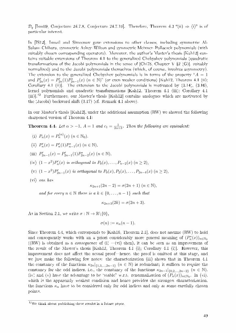
Dq [Ism09, Conjecture 24.7.8, Conjecture 24.7.10]. Therefore, Theorem 4.3 �(ii) ⇒ (i)� is ofparticular interest.

In [IS12], Ismail and Simeonov gave extensions to other classes, including symmetric Al-Salam�Chihara, symmetric Askey�Wilson and symmetric Meixner�Pollaczek polynomials (withsuitably chosen corresponding operators). Moreover, the author's Master's thesis [Kah12] con-tains suitable extensions of Theorem 4.1 to the generalized Chebyshev polynomials (quadratictransformations of the Jacobi polynomials in the sense of [Chi78, Chapter V �2 (G)], suitablynormalized) and to the Jacobi polynomials themselves (which, of course, involves asymmetry).The extension to the generalized Chebyshev polynomials is in terms of the property �A = 1and P ′2n(x) = P ′2n(1)P ∗2n−1(x) (n ∈ N)� (or even weaker conditions) [Kah12, Theorem 4.1 (ii);Corollary 4.1 (ii)]. The extension to the Jacobi polynomials is motivated by (3.14), (3.16),kernel polynomials and quadratic transformations [Kah12, Theorem 4.1 (iii); Corollary 4.1(iii)].42 Furthermore, our Master's thesis [Kah12] contains analogues which are motivated bythe (Jacobi) backward shift (3.17) (cf. Remark 4.1 above).

In our Master's thesis [Kah12], under the additional assumption (RW) we showed the followingsharpened version of Theorem 4.1:

Theorem 4.4. Let α > −1, A = 1 and c1 = 12α+3 . Then the following are equivalent:

(i) Pn(x) = P(α)n (x) (n ∈ N0),

(ii) P ′n(x) = P ′n(1)P ∗n−1(x) (n ∈ N),

(iii) P ′2n−1(x) = P ′2n−1(1)P ∗2n−2(x) (n ∈ N),

(iv) (1− x2)P ′n(x) is orthogonal to P0(x), . . . , Pn−2(x) (n ≥ 2),

(v) (1− x2)P ′2n−1(x) is orthogonal to P0(x), P2(x), . . . , P2n−4(x) (n ≥ 2),

(vi) one hasκ2n+1(2n− 2) = σ(2n+ 1) (n ∈ N),

and for every n ∈ N there is a k ∈ {0, . . . , n− 1} such that

κ2n+3(2k) = σ(2n+ 3).

As in Section 2.1, we write σ : N→ R\{0},

σ(n) := κn(n− 1).

Since Theorem 4.4, which corresponds to [Kah16, Theorem 2.1], does not assume (RW) to holdand consequently works with an a priori considerably more general meaning of (P ∗n(x))n∈N0

((RW) is obtained as a consequence of (i) � (vi) then), it can be seen as an improvement ofthe result of the Master's thesis [Kah12, Theorem 4.1 (i); Corollary 4.1 (i)]. However, thisimprovement does not a�ect the actual proof�hence, the proof is omitted at this stage, andwe just make the following few notes: the characterization (iii) shows that in Theorem 4.1the constancy of the functions κ2n|{1,3,...,2n−1} (n ∈ N) is redundant; it su�ces to require theconstancy for the odd indices, i.e., the constancy of the functions κ2n−1|{0,2,...,2n−2} (n ∈ N).(iv) and (v) have the advantage to be �stable� w.r.t. renormalization of (Pn(x))n∈N0 . In (vi),which is the apparently weakest condition and hence provides the strongest characterization,the functions κn have to be considered only for odd indices and only at some carefully chosenpoints.

42We think about publishing these results in a future paper.

49

In contrast to Theorem 4.1, Theorem 4.4 is no longer a consequence of the results of Hahn andAl-Salam�Chihara mentioned above. The proof of Theorem 4.4 can be found in [Kah16].

In this thesis, we present analogous improvements of Theorem 4.2 and Theorem 4.3. Moreover,we shall give a characterization of a subclass of the continuous q-ultraspherical polynomials interms of the `averaging operator' Aq : R[x] → R[x], which, for every q ∈ (0, 1), is given bylinearity and the de�ning equation

AqTn(x) =qn2 + q−

n2

2Tn(x) (n ∈ N0) (4.10)

[IO11]. We shall also see that this characterization in terms of Aq will not transfer to the wholeclass of continuous q-ultraspherical polynomials.

4.2. A characterization of discrete q-ultraspherical polynomials in terms of theq-di�erence operator

Let A and (Pn(x))n∈N0 be as in Subsection 4.1 (property (RW) is not required), and let q ∈(0, 1). As analogue to (κn)n∈N0 , and following [IO11] (yet with di�erent notation), we considerthe Fourier coe�cients associated with the q-di�erence operator Dq−1 : for every n ∈ N0, letκn(. : q) : N0 → R be given by

κn(k : q) :=

∫RDq−1Pn(x)Pk(x) dµ(x).

It is obvious that κn(k : q) = 0 if k ≥ n or if n − k is even. As analogue to σ, we de�neσ(. : q) : N→ R\{0},

σ(n : q) := κn(n− 1 : q).

The following theorem [Kah16, Theorem 2.2] is the analogue to Theorem 4.4.

Theorem 4.5. Under the conditions of Theorem 4.2, the following are equivalent:

(i) Pn(x) = Pn(x;α : q) (n ∈ N0),

(ii) Dq−1Pn(x) = Dq−1Pn(A)P ∗n−1(x) (n ∈ N),

(iii) Dq−1P2n−1(x) = Dq−1P2n−1(A)P ∗2n−2(x) (n ∈ N),

(iv) (A2 − x2)Dq−1Pn(x) is orthogonal to P0(x), . . . , Pn−2(x) (n ≥ 2),

(v) (A2 − x2)Dq−1P2n−1(x) is orthogonal to P0(x), P2(x), . . . , P2n−4(x) (n ≥ 2),

(vi) one hasκ2n+1(2n− 2 : q) = σ(2n+ 1 : q) (n ∈ N),

and for every n ∈ N there is a k ∈ {0, . . . , n− 1} such that

κ2n+3(2k : q) = σ(2n+ 3 : q).

Since the details of the proof of Theorem 4.5 were omitted in our paper [Kah16] (because theproof is rather similar to the proof of Theorem 4.4�which, however, has been omitted in thisthesis, cf. above), we want to give these details here. We preliminarily note two important(general) relations: on the one hand, the analogue to Lemma 2.4 (i) is

σ(n : q) = q1−n 1− qn

1− q1

cnh(n),

σ(n : q)

σ(n+ 1 : q)= q

1− qn

1− qn+1

ancn

(n ∈ N) (4.11)

50

[IO11, proof of Theorem 4.1].43 On the other hand, (κn(. : q))n∈N0 satis�es the recurrencerelation κ0(. : q) = 0,

anκn+1(k : q) + cnκn−1(k : q) =1

q[akκn(k + 1 : q) + ckκn(k − 1 : q)] +

δn,kh(n)

(n, k ∈ N0) (4.12)

[IO11, proof of Theorem 4.1], which relies on the product rule

Dq[PQ](x) = P (x)DqQ(x) +Q(qx)DqP (x) (P (x), Q(x) ∈ R[x])

[Ism09, (11.4.15)] for Dq.

We now come to the proof of Theorem 4.5. The direction �(i) ⇒ (ii)� is a part of Theorem 4.2,the implications �(ii) ⇒ (iii)� and �(iii) ⇒ (vi)� are trivial. Moreover, (iv) and (v) are obviousreformulations of (ii) and (iii), respectively. It is left to establish �(vi) ⇒ (i)�: we use inductionto show that (4.3) is satis�ed for all n ∈ N if (vi) is assumed to hold. The validity for n = 1 isan assumption of the theorem. Furthermore, (4.12) implies

a2σ(3 : q) + c2σ(1 : q) =A

qσ(2 : q),

which yieldsA

q=

1

q

1− q3

1− q2c2 + q

1− q1− q2

a1

c1c2 =

1

q

1− α2q4

1− q2c2

as a consequence of (4.11). Hence, (4.3) is shown for n = 2. Now let n ∈ N be arbitrary but �xed,and assume that 1, . . . , 2n ful�ll (4.3). Choose k ∈ {0, . . . , n−1} such that κ2n+3(2k : q) = σ(2n+3 : q). Since κ2n(. : q) and κ2n+1(. : q) are uniquely determined by c1, . . . , c2n, we obtain fromthe direction �(i) ⇒ (ii)� (or from Theorem 4.2) that κ2n(2j − 1 : q) = σ(2n : q) (j ∈ {1, . . . , n})and κ2n+1(2j − 2 : q) = σ(2n+ 1 : q) (j ∈ {1, . . . , n+ 1}). Then (4.12) yields

a2n+1κ2n+2(2k + 1 : q) + c2n+1σ(2n : q) =A

qσ(2n+ 1 : q), (4.13)

a2n+1κ2n+2(2n− 1 : q) + c2n+1σ(2n : q) =A

qσ(2n+ 1 : q), (4.14)

a2n+2σ(2n+ 3 : q) + c2n+2σ(2n+ 1 : q) =a2k

qκ2n+2(2k + 1 : q) +

c2k

qκ2n+2(2k − 1 : q), (4.15)

a2n+2σ(2n+ 3 : q) + c2n+2σ(2n+ 1 : q) =a2n

qσ(2n+ 2 : q) +

c2n

qκ2n+2(2n− 1 : q). (4.16)

We distinguish two cases:Case 1: k 6= 0. (4.12) yields

a2n+1κ2n+2(2k − 1 : q) + c2n+1σ(2n : q) =A

qσ(2n+ 1 : q).

43 With regard to the precise relation between (4.11) and Lemma 2.4 (i), we note that the latter would read

σ(n) =n

cnh(n)(n ∈ N)

in the present setting�which can be seen in the same way as in Section 2.3, however. Concerning the variantusing the Christo�el�Darboux formula (cf. (2.20)), take into account that the Christo�el�Darboux formulareads

1

cnh(n)

n−1∑k=0

h(k)P 2k (x) = P ′n(x)Pn−1(x)− P ′n−1(x)Pn(x) (n ∈ N, x ∈ R)

now (cf. [Chi78, I-Theorem 4.6]). Comparing the present setting and the setting which was underlying theoriginal version of Lemma 2.4 (i), the role of a0 is a rather di�erent one: while in the �rst case a0 = A is thenormalization point of the sequence (Pn(x))n∈N0 , in the latter case the normalization point was always 1 andany a0 6= 1 caused asymmetry.

51

Combining this with (4.13) and (4.14), we get κ2n+2(2k+1 : q) = κ2n+2(2k−1 : q) = κ2n+2(2n−1 : q). Hence, (4.15) reduces to

a2n+2σ(2n+ 3 : q) + c2n+2σ(2n+ 1 : q) =A

qκ2n+2(2n− 1 : q). (4.17)

Case 2: k = 0. Here, (4.15) reads a2n+2σ(2n + 3 : q) + c2n+2σ(2n + 1 : q) = Aq κ2n+2(1 : q).

Since (4.13) and (4.14) imply that κ2n+2(1 : q) = κ2n+2(2n− 1 : q), this reduces to (4.17), too.

Note that both in Case 1 and Case 2 the former dependence on k has vanished. We now combine(4.16) and (4.17) and obtain that κ2n+2(2n − 1 : q) = σ(2n + 2 : q). Consequently, (4.14) and(4.17) simplify to

a2n+1σ(2n+ 2 : q) + c2n+1σ(2n : q) =A

qσ(2n+ 1 : q), (4.18)

a2n+2σ(2n+ 3 : q) + c2n+2σ(2n+ 1 : q) =A

qσ(2n+ 2 : q). (4.19)

Applying (4.11) another time, we can deduce from (4.18) that

A

q=

1

q

1− q2n+2

1− q2n+1c2n+1 + q

1− q2n

1− q2n+1

a2n

c2nc2n+1 =

1

q

1− α2q4n+2

1− q2n+1c2n+1,

which shows that (4.3) is satis�ed for 2n+ 1. Knowing this, we �nally can apply (4.11) to (4.19)and obtain

A

q=

1

q

1− q2n+3

1− q2n+2c2n+2 + q

1− q2n+1

1− q2n+2

a2n+1

c2n+1c2n+2 =

1

q

1− α2q4n+4

1− q2n+2c2n+2.

So (4.3) holds true for 2n+ 2, too, which �nishes the induction.

4.3. A characterization of continuous q-ultraspherical polynomials in terms ofthe Askey�Wilson operator

Let A and (Pn(x))n∈N0 be as in Subsection 4.1 again (property (RW) not required), and letq ∈ (0, 1). Following [IO11], we consider as well the Fourier coe�cients w.r.t. the Askey�Wilsonoperator Dq as the Fourier coe�cients w.r.t. the averaging operator Aq and use the followingnotation: for every n ∈ N0, let κn(.|q) : N0 → R and αn(.|q) : N0 → R be de�ned by

κn(k|q) :=

∫RDqPn(x)Pk(x) dµ(x),

αn(k|q) :=

∫RAqPn(x)Pk(x) dµ(x).

Obviously, κn(k|q) = 0 if k ≥ n or if n − k is even, and αn(k|q) = 0 if k ≥ n + 1 or if n − k isodd. As analogue to σ and σ(. : q), we write σ(.|q) : N→ R\{0},

σ(n|q) := κn(n− 1|q).

We have the following analogue [Kah16, Theorem 2.3] to Theorem 4.4 and Theorem 4.5:

Theorem 4.6. Under the conditions of Theorem 4.3, the following are equivalent:

(i) Pn(x) = Pn(x;β|q) (n ∈ N0),

(ii) DqPn(x) = DqPn(A)P ∗n−1(x) (n ∈ N),

(iii) DqP2n−1(x) = DqP2n−1(A)P ∗2n−2(x) (n ∈ N),

52

(iv) (A2 − x2)DqPn(x) is orthogonal to P0(x), . . . , Pn−2(x) (n ≥ 2),

(v) (A2 − x2)DqP2n−1(x) is orthogonal to P0(x), P2(x), . . . , P2n−4(x) (n ≥ 2),

(vi) one hasκ2n+1(2n− 2|q) = σ(2n+ 1|q) (n ∈ N),

and for every n ∈ N there is a k ∈ {0, . . . , n− 1} such that

κ2n+3(2k|q) = σ(2n+ 3|q).

The analogue to Lemma 2.4 (i) and (4.11) is

σ(n|q) = q1−n2

1− qn

1− q1

cnh(n),

σ(n|q)σ(n+ 1|q)

=√q

1− qn

1− qn+1

ancn

(n ∈ N) (4.20)

[IO11, proof of Theorem 5.2].44 The analogue to (4.12) is

anκn+1(k|q) + cnκn−1(k|q) =

(√q

2+

1

2√q

)[akκn(k + 1|q) + ckκn(k − 1|q)] + αn(k|q)

(n, k ∈ N0)

(4.21)

[IO11, proof of Theorem 5.2]; the latter relies on the product rule

Dq[PQ](x) = DqP (x)AqQ(x) +AqP (x)DqQ(x) (P (x), Q(x) ∈ R[x])

[Ism09, (12.1.22)] for Dq.

The proof of Theorem 4.6 is considerably more involved than the proof of Theorem 4.5 (orTheorem 4.4, which can be established by just �copying� the proof of Theorem 4.5 given in theprevious subsection): this is due to the fact that (4.21) is considerably more complicated than(4.12) because (4.21) simultaneously involves the Fourier coe�cients w.r.t. Aq, i.e., (αn(.|q))n∈N0 .To overcome this di�culty, we need several more preliminaries. First, we need the (general)relations

αn(n|q) =qn2 + q−

n2

2h(n)(n ∈ N0), (4.22)

αn(n− 2|q) =(1− q)

(qn−22 − q−

n2

)2︸ ︷︷ ︸

=:Dn

n4 −

∑n−1k=1 ak−1ck

h(n− 2)an−2an−1(n ≥ 2) (4.23)

[IO11, Lemma 5.1].45 Next, we introduce auxiliary functions βn(.|q) : {0, . . . , n− 2} → R,

βn(k|q) :=

∫RAq[xPn(x)]Pk(x) dµ(x) (n ≥ 2),

and use the following result:

Lemma 4.1. For each n ∈ N, the recursion coe�cients c1, . . . , cn determine αn+1(.|q)|{0,...,n}and βn+1(.|q) uniquely.

The proof of Lemma 4.1, which is [Kah16, Lemma 3.1], can be found in our paper [Kah16].Finally, we shall need the following:

44Take into account Footnote 43.45Without going into detail, we note at this stage that the proof of [IO11, Lemma 5.1] given in the cited reference

contains a little mistake concerning the case n = 2. It can easily be corrected by a short calculation.

53

Lemma 4.2. Let β ∈(

0, 1√q

)and Pn(x) = Pn(x;β|q) (n ∈ N0). Then

αn+1(n+ 1− 2k|q)σ(n+ 1|q)

=(β − 1)(1− q)

4√βq

for each n ∈ N and k ∈{

1, . . . ,⌊n+1

2

⌋}.

Our proof of Lemma 4.2, which is [Kah16, Lemma 3.2] and makes use of Theorem 4.3, can befound in [Kah16], too; the special case k = 1 is already contained in [IO11, proof of Theorem 5.2].

We now give a brief sketch of the proof of Theorem 4.6; the details can be found in our paper[Kah16]. As in the proof of Theorem 4.5, the non-obvious part is the implication �(vi) ⇒ (i)�,and we use induction to show that (vi) implies that (4.4) is satis�ed for all n ∈ N. The validityfor n = 1 is clear. Hence, applying the �rst part of Lemma 4.1 and also Lemma 4.2, we have

α2(0|q) =(β − 1)(1− q)

4√βq

σ(2|q).

Now (4.21) yields

a2σ(3|q) + c2σ(1|q) =

(√q

2+

1

2√q

)Aσ(2|q) + α2(0|q) =

1

2

(√β

q+

√q

β

)σ(2|q);

applying (4.20), we get

1

2

(√β

q+

√q

β

)=

1− q3

√q(1− q2)

c2 +

√q

1 + q

a1

c1c2 =

(√β

q+

√q

β

)1− βq2

√β(1− q2)

c2.

Consequently, (4.4) holds true for n = 2. Let n ∈ N be arbitrary but �xed, assume that 1, . . . , 2nsatisfy (4.4), and choose k ∈ {0, . . . , n − 1} such that κ2n+3(2k|q) = σ(2n + 3|q). In a similarway as in the proof of Theorem 4.5�and taking into account as well the �rst part of Lemma 4.1as Lemma 4.2�we obtain

a2n+2σ(2n+ 3|q) + c2n+2σ(2n+ 1|q) =

=

(√q

2+

1

2√q

)[a2nσ(2n+ 2|q) + c2nκ2n+2(2n− 1|q)] + α2n+2(2n|q),

(4.24)

and

a2n+2σ(2n+ 3|q) + c2n+2σ(2n+ 1|q) =

(√q

2+

1

2√q

)Aκ2n+2(2n− 1|q) + α2n+2(2k|q), (4.25)

as analogues to (4.16) and (4.17).

At this stage, an important di�erence to the proof of Theorem 4.5 occurs: in contrast to (4.17),in (4.25) the dependence on k has not vanished. Furthermore, α2n+2(2k|q) in (4.25) is notdetermined by the induction hypothesis (i.e., c1, . . . , c2n), nor is α2n+2(2n|q) in (4.24). In contrastto the proof of Theorem 4.5 and the equations (4.16) and (4.17), (4.24) and (4.25) do notimmediately yield the (potentially helpful) conclusion κ2n+2(2n−1|q) = σ(2n+2|q) (nevertheless,the latter will turn out to be true later). These circumstances are the actual di�culty in theproof of Theorem 4.6. The key idea to overcome these problems consists of the following threeingredients:

� via (4.23), relate α2n+2(2n|q) to α2n+1(2n − 1|q), which�due to the �rst part ofLemma 4.1�is determined by the induction hypothesis;

54

� consider the auxiliary function β2n+1(.|q), apply the induction hypothesis and the secondpart of Lemma 4.1 to β2n+1(2k|q) and relate it to α2n+2(2k|q) via a2n+1α2n+2(2k|q) =β2n+1(2k|q)− c2n+1α2n(2k|q);

� simultaneously involve the sequence (Pn(x;β|q))n∈N0 of continuous q-ultraspherical poly-nomials itself�from now on, we write an additional tilde when explicitly referring to

(Pn(x;β|q))n∈N0 (in particular, c2n+1

(=√β

21−q2n+1

1−βq2n+1

)).

Without going into detail, we note that this approach yields

a2n+1α2n+2(2n|q)σ(2n+ 1|q)

=(1− q)2

2qa2n︸ ︷︷ ︸

=:A1(n)

c2n+1 +(β − 1)(1− q)

4√βq

D2n+2

D2n+1c2n −

(1− q)2

8q︸ ︷︷ ︸=:A2(n)

(4.26)

and

a2n+1α2n+2(2k|q)σ(2n+ 1|q)

=−(β − 1)(1− q)4√β

1− q2n

1− q2n+1

a2n

c2n︸ ︷︷ ︸=:A3(n)

c2n+1

+(β − 1)(1− q)

4√β(q − q2n+2)

[(1− q2n+2) + (q − q2n+1)

a2n

c2n

]c2n+1︸ ︷︷ ︸

=:A4(n)

.

(4.27)

Moreover (again we skip any details), the di�erence of (4.24) and (4.25) simpli�es to

a2n+1α2n+2(2n|q)σ(2n+ 1|q)

− a2n+1α2n+2(2k|q)σ(2n+ 1|q)

=

= − q + 1

2(q − q2n+2)a2n

[(1− q2n+2) + (q − q2n+1)

a2n

c2n

]︸ ︷︷ ︸

=:A5(n)

c2n+1 +(β + q)(q + 1)

4q√β

a2n︸ ︷︷ ︸=:A6(n)

.(4.28)

Combining (4.26), (4.27) and (4.28), we obtain

[A1(n)−A3(n)−A5(n)]c2n+1 = −[A2(n)−A4(n)−A6(n)], (4.29)

where the former dependence on k has vanished now. A1(n), . . . , A6(n) are determined by theinduction hypothesis, and

A1(n)−A3(n)−A5(n) 6= 0 (4.30)

(the latter can be seen by a short elementary calculation). Hence, we could compute c2n+1 asthe quotient −A2(n)−A4(n)−A6(n)

A1(n)−A3(n)−A5(n) , which�after tedious calculations�would yield the desiredresult.

However, also a much faster argument is available at this stage: as an immediate consequenceof the already veri�ed direction �(i) ⇒ (vi)� (or of Theorem 4.3), the argument up to this pointwould remain valid if (Pn(x))n∈N0 was replaced by (Pn(x;β|q))n∈N0 ; hence, (4.29) would remainvalid if c2n+1 was replaced by c2n+1. So

[A1(n)−A3(n)−A5(n)](c2n+1 − c2n+1) = 0.

Consequently, c2n+1 = c2n+1, i.e., (4.4) is valid for 2n+ 1.46

46This �replacement argument� has another advantage: it would not even have been necessary to compute A2(n),

A4(n) and A6(n) as above; instead, it would have been enough to observe thata2n+1α2n+2(2n|q)

σ(2n+1|q) −A1(n)c2n+1,a2n+1α2n+2(2k|q)

σ(2n+1|q) − A3(n)c2n+1 anda2n+1α2n+2(2n|q)

σ(2n+1|q) − a2n+1α2n+2(2k|q)σ(2n+1|q) − A5(n)c2n+1 are �xed by c1, . . . , c2n.

The values of A1(n), A3(n) and A5(n) (which are also determined by c1, . . . , c2n) are only needed to show(4.30).

55

Since besides c1, . . . , c2n also c2n+1 is known now, Lemma 4.1 and Lemma 4.2 imply that both(4.24) and (4.25) reduce to

a2n+2σ(2n+ 3|q) + c2n+2σ(2n+ 1|q) =1

2

(√β

q+

√q

β

)σ(2n+ 2|q). (4.31)

Following the remaining proof of Theorem 4.5, we can deduce from (4.31) that (4.4) is valid for2n+ 2, too, which �nishes the induction.

4.4. A characterization of continuous q-ultraspherical polynomials in terms ofthe averaging operator

Let A and (Pn(x))n∈N0 be as in Subsection 4.1 another time (property (RW) not required), letq ∈ (0, 1) again, and use the notation of the previous subsection. The following theorem [Kah16,Theorem 2.4] is the announced characterization in terms of the averaging operator Aq:

Theorem 4.7. Under the conditions of Theorem 4.3 and the additional assumption that β ≤ 1,the following are equivalent:

(i) Pn(x) = Pn(x;β|q) (n ∈ N0),

(ii) the quotient αn+1(n−1|q)σ(n+1|q)

(=∫RAqPn+1(x)Pn−1(x) dµ(x)∫RDqPn+1(x)Pn(x) dµ(x)

)is independent of n ∈ N.

If the condition β ≤ 1 is dropped, then only �(i) ⇒ (ii)� remains valid.

Besides the averaging operator Aq, Theorem 4.7 involves σ(n + 1|q) (and consequently theAskey�Wilson operator Dq). However, recall that σ(n + 1|q) can be expressed in terms of therecurrence coe�cients in a considerably more convenient way than the analogue concerningαn+1(n−1|q), cf. (4.20) and (4.23). Therefore, we think it is indeed justi�ed to call Theorem 4.7a characterization �in terms of the averaging operator�.

We brie�y sketch the proof of Theorem 4.7 (and refer to our paper [Kah16] for the details again):�rst not imposing the additional condition β ≤ 1, the implication �(i) ⇒ (ii)� is an obviousconsequence of Lemma 4.2, and�using (4.20) and (4.23)�we can reformulate (ii) as[

an +1− β

2√β(1− q)

1− qn+2

1− qn+1

]cn+1 =

1

4+

1− β2√β(1− q)

1− qn+1

1− qncn (n ∈ N). (4.32)

Now assume that (ii) is satis�ed, and also that β ≤ 1. We use induction to verify (4.4) for alln ∈ N: this is clear for n = 1, so let n ∈ N be arbitrary but �xed and assume (4.4) to be satis�edfor n. Short calculations yield

an +1− β

2√β(1− q)

1− qn+2

1− qn+1=

1− βqn+1

2√β(1− qn+1)

2− q − qn+1 − (1 + qn − 2qn+1)β

(1− q)(1− βqn)(4.33)

and1

4+

1− β2√β(1− q)

1− qn+1

1− qncn =

2− q − qn+1 − (1 + qn − 2qn+1)β

4(1− q)(1− βqn). (4.34)

Since β ≤ 1, we have2− q − qn+1 − (1 + qn − 2qn+1)β 6= 0. (4.35)

Hence, combining (4.32), (4.33), (4.34) and (4.35), we obtain that (4.4) is also valid for n + 1,which �nishes the induction.

56

Concerning the second part of the theorem (i.e., that �(ii) ⇒ (i)� is not generally true if the

additional assumption β ≤ 1 is dropped), via A := 94√

5, c1 :=

√5

3 , c2 := 12 ,

cn+1 :=

√5− 2n+1−1

2n−1 cn

9− 4√

5cn − 2n+2−12n+1−1

(n ≥ 2)

one can recursively de�ne a symmetric RWPS (Pn(x))n∈N0 such that, putting q := 12 and β := 5

4 ,the conditions of Theorem 4.3 and (ii) are satis�ed. However, (Pn(x))n∈N0 6= (Pn(x;β|q))n∈N0

because c2 = 12 6=

3√

511 =

√β

21−q2

1−βq2 (cf. (4.4)).

Remark 4.2. Although the condition β ≤ 1 cannot be completely removed, the equivalence �(i)⇔ (ii)� of Theorem 4.7 remains valid if β ≤ 1 is replaced by one of the weaker conditions

∀n ∈ N :2− q − qn+1

1 + qn − 2qn+16= β,

∀n ∈ N :

(2− q − qn+1

1 + qn − 2qn+1= β ⇒ cn+1 =

√β

2

1− qn+1

1− βqn+1

),

cf. the detailed proof of Theorem 4.7 given in our paper [Kah16]. Since the function

(0,∞) → (1,∞), x 7→ 2−q−qx+1

1+qx−2qx+1 is strictly increasing, there exists at most one n ∈ N such

that 2−q−qn+1

1+qn−2qn+1 = β, and if β ≤ 1, then there is none.

Remark 4.3. The ultraspherical polynomials appear as limiting cases of as well the discrete asthe continuous q-ultraspherical polynomials (cf. Subsection 4.1); consequently, it is a naturalquestion to ask whether Theorem 4.5 or Theorem 4.6 implies Theorem 4.4 by just �taking thelimit� q → 1. However, there is no obvious reason why the �characterizing� directions �(vi) ⇒(i)� should remain valid if one passes to limits. The same is the case w.r.t. the original results ofLasser�Obermaier and Ismail�Obermaier: the directions �(ii)⇒ (i)� of Theorem 4.1, Theorem 4.2and Theorem 4.3 are mutually independent from each other.In this context, we make the following observation w.r.t. Theorem 4.7: let α > −1. There existssome q0 ∈ [0, 1) such that 2−q−qn+1

1+qn−2qn+1 6= qα+ 12 for all n ∈ N and q ∈ (q0, 1).47 Hence, if q ∈ (q0, 1),

if A =

√qα+

12

2 + 1

2

√qα+

12

, if c1 =

√qα+

12

21−q

1−qα+32and if αn+1(n−1|q)

σ(n+1|q) is independent of n ∈ N, then

Pn(x) = Pn(x; qα+ 12 |q) (n ∈ N0) as a consequence of Theorem 4.7 and Remark 4.2.48 Despite

the fact that limq→1 Pn(x; qα+ 12 |q) = P

(α)n (x) (n ∈ N0, x ∈ R) (4.5), the �limiting conditions�

A = 1, c1 = 12α+3 and �0 is independent of n ∈ N� do not enforce that Pn(x) = P

(α)n (x) (n ∈ N0),

of course. Since the limiting case of Theorem 4.7 (ii) is a trivial property that is always true(because Aq becomes the identity as q → 1), one has no analogue to Theorem 4.7 for the classof ultraspherical polynomials.

47This can be seen as follows: let u, v : (0, 1) → R be de�ned by u(q) := 2 − q − qα+12 , v(q) := q + qα+

12 −

2qα+32 . Since limq→1 u(q) = limq→1 v(q) = 0, and since u and v are continuously di�erentiable on (0, 1) with

limq→1 u′(q) = limq→1 v

′(q) = −α − 32< 0, there exists some q∗0 ∈ (0, 1) such that u(q) > 0 and v(q) > 0

for all q ∈ [q∗0 , 1). Now consider the function w : [q∗0 , 1) → R, w(q) :=log

u(q)v(q)

log q. After several applications of

L'Hôpital's rule, one sees that w converges to a real number if q → 1 (in fact, limq→1 w(q) = − 4α+22α+3

). So w isbounded; in particular, there exists some N ∈ N such that n > w(q) for all q ∈ [q∗0 , 1) and n ∈ N with n > N .

The latter is easily seen to imply that 2−q−qn+1

1+qn−2qn+1 > qα+12 for all q ∈ [q∗0 , 1) and n ∈ N with n > N . Since

each of the functions (0, 1) → R, q 7→ 2−q−qn+1

1+qn−2qn+1 − qα+12 , n ∈ {1, . . . , N}, has at most �nitely many zeros,

we obtain indeed some q0 ∈ [0, 1) with the desired property.48In the special case α ≥ − 1

2, the argument considerably simpli�es because qα+

12 ≤ 1 then; consequently, one

can apply Theorem 4.7 in its original formulation (and does not have to take into account Remark 4.2), andone may choose q0 = 0.

57

Outlook

One of the things that make science and research so interesting and exciting is that every solvedproblem immediately leads to new questions. This short section is devoted to some suggestionsfor future research. We �rst present some ideas without going into detail, and then brie�ydiscuss two selected problems from which we think that they are of particular interest�andwhich we plan to solve in the course of our postdoctoral research.

In Section 2, we considered polynomial hypergroups and obtained a su�cient criterion (Theo-rem 2.1) and a necessary criterion (Theorem 2.2) for weak amenability of their `1-algebras `1(h).This enabled us to characterize weak amenability (and also point amenability) for the classes ofJacobi polynomials (Theorem 3.1), symmetric Pollaczek polynomials (Theorem 3.2), associatedultraspherical polynomials (Theorem 3.3), random walk polynomials (in the sense of Section 3;Proposition 3.1) and cosh-polynomials (Proposition 3.2). Also the notions of amenabilityand right character amenability are solved problems concerning theses classes, cf. Section 3.However, it would be interesting to clarify the situation w.r.t. approximate amenability (which,since `1(h) is commutative and unital, coincides with pseudo-amenability and implies weakamenability), w.r.t. pointwise amenability (which implies approximate amenability at thisstage) or w.r.t. other amenability notions for Banach algebras (cf. Section 1.2 and Section 1.4).Recall that the problem of pointwise amenability seems to be open even for L1-algebras oflocally compact groups.

It would also be interesting to study more general structures (for instance, hypergroupswhich are not located at the fruitful crossing point to the theory of orthogonal polynomials),or to study further examples of polynomial hypergroups. Concerning the latter, there is avery interesting class which comes from q-calculus and for which property (P), as well asright character amenability of `1(h), are known to hold: this is the class of little q-Legendrepolynomials, and we shall discuss it in some more detail below (as the �rst of the two selectedproblems mentioned above).

Recall that, in accordance with previous research on polynomial hypergroups and their`1-algebras, we considered point derivations (and also the concepts of α- and ϕ-amenability)w.r.t. Hermitian characters. There are good reasons for this restriction: on the one hand,the general theory and the available harmonic analysis becomes richer (cf. Abelian locallycompact groups). On the other hand, for our main examples (Jacobi, symmetric Pollaczekand associated ultraspherical polynomials) all characters are Hermitian. Nevertheless, thegeneral question about non-symmetric characters suggests interesting problems: for instance,it is an interesting question to ask whether there holds a more general version�concerningnon-symmetric characters�of the full assertion of Proposition 2.1 (i) (whose proof essentiallyrelied on the boundedness of the derivatives of the Chebyshev polynomials of the second kind

at each x ∈ (−1, 1)): since the set

{d

dxP( 12)

n (x) : n ∈ N0

}is unbounded for every x ∈ C\(−1, 1)

(use (3.16) and the fact that N0 = X b(N0) = supp µ = [−1, 1] for the sequence

(P

( 32)

n (x)

)n∈N0

),

at least the proof of Proposition 2.1 (i) breaks down as soon as one does not restrict oneselfto Hermitian characters. Moreover, we cannot draw any conclusion concerning the size ofX b(N0)\N0 (because the equalities N0 = X b(N0) = supp µ = [−1, 1] are also valid for theChebyshev polynomials of the second kind).

With regard to Theorem 4.5, Theorem 4.6 and Theorem 4.7: results of our Master's thesis[Kah12] (cf. Section 4.1) suggest to look for generalizations to suitable q-analogues of the Jacobiand generalized Chebyshev polynomials, and the results of Ismail�Simeonov [IS12] suggest to

58

look for generalizations to symmetric Al-Salam�Chihara, symmetric Askey�Wilson, symmetricMeixner�Pollaczek or more abstract symmetric orthogonal polynomials. In particular, we planto establish a characterization which is motivated by a certain q-extension of the generalizedChebyshev polynomials considered in [Mej10] (as another possible part of our PostDoc research).Our Master's thesis [Kah12] also suggests research motivated by the �backward shift analogues�(cf. [KLS10, (14.5.9)] and [KLS10, (14.10.25)], and cf. Section 4.1). However, we are evenmore interested in another type of generalization�which is very di�erent from the situationsstudied in [IS12] and [Kah12]: this problem concerns sieved orthogonal polynomials and certain�limiting operators� of Dq and Aq; we shall discuss it in some more detail below (as the secondof the two selected problems mentioned above).

We now come to the announced details:

� Concerning both our su�cient criterion Theorem 2.1 and our necessary criterion The-orem 2.2 for weak amenability of `1-algebras of polynomial hypergroups, absolutecontinuity of the orthogonalization measure plays a crucial role. For instance, theproof of Theorem 2.1 relied on the fundamental lemma of the calculus of variations,and the proof of Theorem 2.2 made use of an integration by parts argument for theRadon�Nikodym derivatives. Considering purely discrete orthogonalization measures, theproof of Theorem 2.1 breaks down for several reasons; for instance, an application of theessential ingredient [MNT87, Theorem 12.1] on limiting behavior is no longer possible.

An important example of a polynomial hypergroup with purely discrete orthogonalizationmeasure is provided by the little q-Legendre polynomials: given q ∈ (0, 1), the corre-sponding sequence (Rn(x; q))n∈N0 of little q-Legendre polynomials is determined by theorthogonalization measure

µ(x) =

{qn(1− q), x = 1− qn with n ∈ N0,

0, else

and the normalization Rn(1; q) = 1 (n ∈ N0), or, equivalently, via

a0 =1

q + 1, an = qn

(1 + q)(1− qn+1)

(1− q2n+1)(1 + qn+1)(n ∈ N),

cn = qn(1 + q)(1− qn)

(1− q2n+1)(1 + qn)(n ∈ N),

bn ≡ 1− an − cn.

(4.36)

Property (P) is always satis�ed, so a polynomial hypergroup is induced. One has

h(n) =1

qn1− q2n+1

1− q(n ∈ N0) (4.37)

and N0 = X b(N0) = supp µ = {1}∪ {1− qn : n ∈ N0}. Consequently, Reiter's condition P2

is satis�ed. These basics are taken from [KLS10, Section 14.12.1], [Las05, Section 6] and[Las09b, Example 3]. Applying Lemma 2.4 (i), we obtain

σ(n) =(1− q)(1 + qn)

1− qnn (n ∈ N). (4.38)

As we already have recalled, the corresponding `1-algebra `1(h) is right character amenable(and consequently point amenable, cf. also [Las09b, Example 3]) yet non-amenable; whileright character amenability follows from the fact that the hypergroup is `of strong compact

59

type' [FLS05], non-amenability is an immediate consequence of (4.37) and Theorem 1.4 (i).

Obviously, our su�ciency criterion Theorem 2.1 cannot be applied to establish weakamenability of `1(h). Moreover, the situation is consistent with our necessary criterionTheorem 2.2: in view of (4.38) and the �rst part of Theorem 2.2, neither (i) nor (ii) ofTheorem 2.2 is violated.

Recall that our strategy for the proof of Theorem 2.1 relied on the sequence (Fn)n∈N0 ⊆ c00

(cf. (2.1) and (2.2)), on a speci�c certain limit F of this sequence (speci�c in the sensethat the limit contains adequate information about the individual underlying sequenceof orthogonal polynomials), and on a density argument concerning the linear span ofthe set {TmF : m ∈ N0}. Concerning the little q-Legendre polynomials, this approachbreaks down at least for the following two reasons: on the one hand, (4.36) yields that(Rn(x; q))n∈N0 is of `Nevai class M(1, 0)', i.e., αn → 0 (n → ∞) and βn → 1 (n → ∞)(cf. the recurrence relation for the orthonormal sequence (pn(x))n∈N0). Applying anotherresult of Nevai on limiting behavior [Nev79, Lemma 4.2.9, Theorem 4.2.10], this impliesthat (Fn)n∈N0 converges pointwise to the trivial character 1α�however, the trivialcharacter is not speci�c to (Rn(x; q))n∈N0 in any way; in other words: passing to the limitis accompanied by a considerable loss of information. On the other hand, and this is theeven more serious aspect, Tm 1α = 1α for every m ∈ N0 (1.10)�consequently, the linearspan of {Tm 1α : m ∈ N0} is only one-dimensional.

For these reasons, we think that the question of whether the little q-Legendre polynomi-als bear weakly amenable `1-algebras or not is a rather nontrivial one. We plan to solvethis problem with completely di�erent methods�as a possible project for our PostDocresearch�and do not go into further detail at this stage; we just mention that we have theconjecture that the `1-algebras are weakly amenable, and that we think that the asymp-totics of the little q-Legendre polynomials [IW82] will play a crucial role for the solution.49

� Let (Pn(x))n∈N0 ⊆ R[x] be a symmetric RWPS (in the sense of Section 4) with normaliza-tion point 1, i.e., (Pn(x))n∈N0 is given by a recurrence relation of the form P0(x) = 1,

xPn(x) = anPn+1(x) + cnPn−1(x) (n ∈ N0),

where c0 := 0, (cn)n∈N ⊆ (0, 1) and an := 1−cn (n ∈ N0). Let k ∈ N, and let (Pn(x; k))n∈N0

denote the `k-sieved RWPS' which corresponds to (Pn(x))n∈N0 , i.e., P0(x; k) = 1 and

xPn(x; k) = a(n; k)Pn+1(x; k) + c(n; k)Pn−1(x; k) (n ∈ N0)

with

c(n; k) :=

{cnk, k|n,

12 , else

and a(n; k) := 1− c(n; k) (n ∈ N0); sometimes the additional expression �of the �rst kind�is used.50 Sieved RWPS have been studied in [GVA88] and in [IL92] (the latter being partof a series of papers by Ismail et al.), for instance.

49Note that if the conjecture is true, one obtains as an obvious consequence that not all of the conditions (i) �(iv) of our su�ciency criterion Theorem 2.1 are necessary for weak amenability of `1(h) (cf. the notes at theend of Section 3.2).

50However, the expression �of the �rst kind� does also appear with a di�erent meaning (in the context of certainsieved polynomials).

60

If Pn(x) = P(α)n (x) (n ∈ N0) for some α > −1, then (Pn(x; k))n∈N0 is given by

Pn(x; k) = lims→1

Pn

(x; sαk+ k

2 |se2πik

)(4.39)

for every n ∈ N0 and x ∈ R [ASAA84], and we write (P(α)n (x; k))n∈N0 for these `k-sieved

ultraspherical polynomials'. Of course, (4.39) requires a more general de�nition of thecontinuous q-ultraspherical polynomials (Pn(x;β|q))n∈N0 than considered in Section 4(in particular, allowing q to be non-real, and allowing the moment functionals to be notnecessarily restricted to the positive-de�nite case; we refrain from going into too muchdetail at this stage). Observe that (4.39) generalizes (4.5).

Having in mind (4.39), in view of Theorem 4.1 and Theorem 4.3 it is a natural questionto ask whether there exists an analogous characterization of the k-sieved ultrasphericalpolynomials in terms of the �k-sieved Askey�Wilson operator� Dk : R[x]→ R[x] which weintroduce via

DkTn(x) := lims→1

(√se

2πik

)n−(√

se2πik

)−n√se

2πik − 1√

se2πik

Un−1(x) = Un−1

(∣∣∣cosπ

k

∣∣∣)Un−1(x) (n ∈ N0)

(cf. (4.9) and (4.2)) and linear extension. Moreover, in view of Theorem 4.7 it is aninteresting problem whether there exists an analogous characterization of the k-sievedultraspherical polynomials in terms of the �k-sieved averaging operator� Ak : R[x]→ R[x]which we introduce via

AkTn(x) := lims→1

(√se

2πik

)n+(√

se2πik

)−n2

Tn(x) = Tn

(∣∣∣cosπ

k

∣∣∣)Tn(x) (n ∈ N0)

(cf. (4.10) and (2.5)) and linear extension.

For k ≥ 2, which shall be assumed from now on,51 at �rst sight it might indeed seemreasonable to expect such analogous characterizations in terms of Dk and Ak.

However, these �sieved operators� are very di�erent from ddx , Dq and Aq�and also from Dq,

and from the operators corresponding to the Ismail�Simeonov characterizations in [IS12]�for the reason that Dk and Ak have in�nite-dimensional kernels (because Un−1

(∣∣cos πk∣∣) =

Un−1

(cos πk

)becomes zero for in�nitely many n ∈ N0 (4.2), as well as Tn

(∣∣cos πk∣∣) =

Tn(cos πk

)becomes zero for in�nitely many n ∈ N0 (2.5)). This important observation

gives reason to expect a certain loss of information, or, in other words, an additional degreeof freedom. We plan to solve this problem as another possible project for our PostDocresearch and hence do not go into further detail at this stage; we just mention that wehave the conjecture that (still assuming k ≥ 2) analogues of Theorem 4.1, Theorem 4.3and Theorem 4.7 do not yield characterizations of the k-sieved ultraspherical polynomialsbut characterizations of arbitrary k-sieved RWPS.52

51The case k = 1 is obvious because D1 = ddx

(4.8) and A1 = id: while there is a characterization of the 1-sieved ultraspherical polynomials�i.e., the ultraspherical polynomials themselves�in terms of D1, namelyjust Theorem 4.1 itself, there is no analogue to Theorem 4.7 in terms of A1 (cf. also Remark 4.3). Note thatthe formal limit �D∞� coincides with D1, as well as �A∞� coincides with A1.

52We call a symmetric RWPS `k-sieved' (without further speci�cation) if it is k-sieved w.r.t. another symmetricRWPS (or, equivalently, if cn = 1

2if k 6 |n).

61

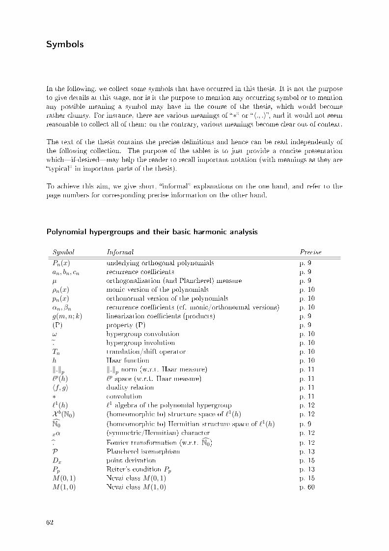
Symbols

In the following, we collect some symbols that have occurred in this thesis. It is not the purposeto give details at this stage, nor is it the purpose to mention any occurring symbol or to mentionany possible meaning a symbol may have in the course of the thesis, which would becomerather clumsy. For instance, there are various meanings of �∗� or �〈., .〉�, and it would not seemreasonable to collect all of them: on the contrary, various meanings become clear out of context.

The text of the thesis contains the precise de�nitions and hence can be read independently ofthe following collection. The purpose of the tables is to just provide a concise presentationwhich�if desired�may help the reader to recall important notation (with meanings as they are�typical� in important parts of the thesis).

To achieve this aim, we give short, �informal� explanations on the one hand, and refer to thepage numbers for corresponding precise information on the other hand.

Polynomial hypergroups and their basic harmonic analysis

Symbol Informal Precise

Pn(x) underlying orthogonal polynomials p. 9an, bn, cn recurrence coe�cients p. 9µ orthogonalization (and Plancherel) measure p. 9ρn(x) monic version of the polynomials p. 10pn(x) orthonormal version of the polynomials p. 10αn, βn recurrence coe�cients (cf. monic/orthonormal versions) p. 10g(m,n; k) linearization coe�cients (products) p. 9(P) property (P) p. 9ω hypergroup convolution p. 10. hypergroup involution p. 10Tn translation/shift operator p. 10h Haar function p. 10‖.‖p ‖.‖p-norm (w.r.t. Haar measure) p. 11`p(h) `p-space (w.r.t. Haar measure) p. 11〈f, g〉 duality relation p. 11∗ convolution p. 11`1(h) `1-algebra of the polynomial hypergroup p. 12X b(N0) (homeomorphic to) structure space of `1(h) p. 12N0 (homeomorphic to) Hermitian structure space of `1(h) p. 9

xα (symmetric/Hermitian) character p. 12. Fourier transformation (w.r.t. N0) p. 12P Plancherel isomorphism p. 13Dx point derivation p. 15Pp Reiter's condition Pp p. 13M(0, 1) Nevai class M(0, 1) p. 15M(1, 0) Nevai class M(1, 0) p. 60

62

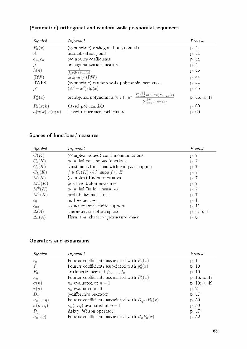
(Symmetric) orthogonal and random walk polynomial sequences

Symbol Informal Precise

Pn(x) (symmetric) orthogonal polynomials p. 44A normalization point p. 44an, cn recurrence coe�cients p. 44µ orthogonalization measure p. 44h(n) 1∫

RP2n(x) dµ(x)

p. 46

(RW) property (RW) p. 44RWPS (symmetric) random walk polynomial sequence p. 44µ∗ (A2 − x2) dµ(x) p. 45

P ∗n(x) orthogonal polynomials w.r.t. µ∗;∑bn2 ck=0 h(n−2k)Pn−2k(x)∑bn2 c

k=0 h(n−2k)p. 45; p. 47

Pn(x; k) sieved polynomials p. 60a(n; k), c(n; k) sieved recurrence coe�cients p. 60

Spaces of functions/measures

Symbol Informal Precise

C(K) (complex-valued) continuous functions p. 7Cb(K) bounded continuous functions p. 7Cc(K) continuous functions with compact support p. 7CE(K) f ∈ Cc(K) with supp f ⊆ E p. 7M(K) (complex) Radon measures p. 7M+(K) positive Radon measures p. 7M b(K) bounded Radon measures p. 7M1(K) probability measures p. 7c0 null sequences p. 11c00 sequences with �nite support p. 11∆(A) character/structure space p. 4; p. 4∆s(A) Hermitian character/structure space p. 6

Operators and expansions

Symbol Informal Precise

εn Fourier coe�cients associated with Pn(x) p. 11fn Fourier coe�cients associated with p2

n(x) p. 19Fn arithmetic mean of f0, . . . , fn p. 19κn Fourier coe�cients associated with P ′n(x) p. 16; p. 47σ(n) κn evaluated at n− 1 p. 19; p. 49τ(n) κn evaluated at 0 p. 24Dq q-di�erence operator p. 47κn(. : q) Fourier coe�cients associated with Dq−1Pn(x) p. 50σ(n : q) κn(. : q) evaluated at n− 1 p. 50Dq Askey�Wilson operator p. 47κn(.|q) Fourier coe�cients associated with DqPn(x) p. 52

63

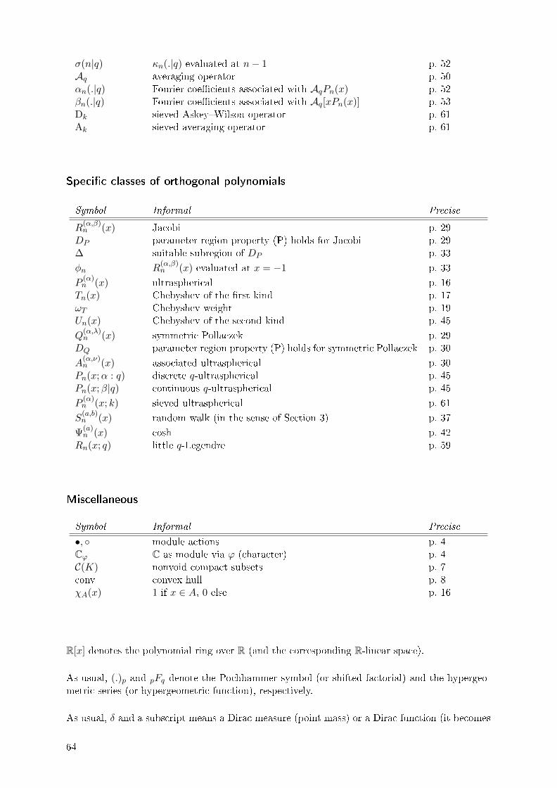
σ(n|q) κn(.|q) evaluated at n− 1 p. 52Aq averaging operator p. 50αn(.|q) Fourier coe�cients associated with AqPn(x) p. 52βn(.|q) Fourier coe�cients associated with Aq[xPn(x)] p. 53Dk sieved Askey�Wilson operator p. 61Ak sieved averaging operator p. 61

Speci�c classes of orthogonal polynomials

Symbol Informal Precise

R(α,β)n (x) Jacobi p. 29

DP parameter region property (P) holds for Jacobi p. 29∆ suitable subregion of DP p. 33

φn R(α,β)n (x) evaluated at x = −1 p. 33

P(α)n (x) ultraspherical p. 16Tn(x) Chebyshev of the �rst kind p. 17ωT Chebyshev weight p. 19Un(x) Chebyshev of the second kind p. 45

Q(α,λ)n (x) symmetric Pollaczek p. 29

DQ parameter region property (P) holds for symmetric Pollaczek p. 30

A(α,ν)n (x) associated ultraspherical p. 30

Pn(x;α : q) discrete q-ultraspherical p. 45Pn(x;β|q) continuous q-ultraspherical p. 45

P(α)n (x; k) sieved ultraspherical p. 61

S(a,b)n (x) random walk (in the sense of Section 3) p. 37

Ψ(a)n (x) cosh p. 42

Rn(x; q) little q-Legendre p. 59

Miscellaneous

Symbol Informal Precise

•, ◦ module actions p. 4Cϕ C as module via ϕ (character) p. 4C(K) nonvoid compact subsets p. 7conv convex hull p. 8χA(x) 1 if x ∈ A, 0 else p. 16

R[x] denotes the polynomial ring over R (and the corresponding R-linear space).

As usual, (.)p and pFq denote the Pochhammer symbol (or shifted factorial) and the hypergeo-metric series (or hypergeometric function), respectively.

As usual, δ and a subscript means a Dirac measure (point mass) or a Dirac function (it becomes

64

clear out of context whether a Dirac measure or a Dirac function shall be meant). We also usethe well-known Kronecker delta.

For the sake of completeness and to avoid any confusion, we note that the set N shall not contain0 (if 0 shall be contained, we write N0).

65

A. Publication [Kah15]

A.1. Summary

In our paper [Kah15] (sole author), we study two amenability properties for `1-algebras ofpolynomial hypergroups: on the one hand, we are interested in `weak amenability' of these`1-algebras, i.e., in the nonexistence of nonzero bounded derivations into `∞; on the otherhand, we consider the nonexistence of nonzero bounded point derivations w.r.t. symmetriccharacters (regarded as a global property, `point amenability'). Originally coming from abstractharmonic and functional analysis (cohomology), it is known that these properties correspondto questions concerning the derivatives of the underlying orthogonal polynomials (Pn(x))n∈N0

and concerning certain associated Fourier coe�cients (Lasser 2007, 2009). Despite these ratherconcrete correspondencies, deciding whether a given polynomial hypergroup bears a weakly orpoint amenable `1-algebra requires often deep knowledge about (Pn(x))n∈N0 .

Polynomial hypergroups are interesting for several reasons. In our opinion, the most importantmotivation for considering these structures is that they o�er an elegant possibility to studyorthogonal polynomials via methods from functional and harmonic analysis�in particular, viathe machinery provided by Gelfand theory; for instance, the Hermitian characters can be iden-ti�ed with a compact subset of R which contains the support of the orthogonalization measure.On the other side of the coin, polynomial hypergroups provide an abundance of interestinghypergroups (and corresponding L1-algebras) which are based on the theory of orthogonalpolynomials and special functions, and which are very di�erent from any locally compact group.For instance, even point amenability�which is the weaker of the two amenability propertieswe focus on in [Kah15]�is often not satis�ed for `1-algebras of polynomial hypergroups (incontrast to the group case). The results of [Kah15] can be divided into two parts: in Section2, we give some general results on point and weak amenability of `1-algebras of polynomialhypergroups, whereas from Section 3 on we consider concrete examples and, in particular,obtain characterizations of these amenability properties for the classes of Jacobi polynomials(Theorem 3.1), symmetric Pollaczek polynomials (Theorem 4.1) and associated ultrasphericalpolynomials (Theorem 5.1) as main results�by identifying the corresponding parameter regionsin each case. In doing so, we shall also obtain examples of polynomial hypergroups with weaklyamenable but non-amenable `1-algebra (e.g., certain ultraspherical polynomials), which solves aproblem which has been open for some years.

The main results of Section 2 are a necessary criterion (Theorem 2.2) and a su�cient criterion(Theorem 2.3) for weak amenability; later in the paper, we will apply these to situations wheremore explicit computations seem to be out of reach. The criteria and their proofs use shift oper-ators, certain regularity and smoothness conditions on the orthogonalization measures, growthconditions (e.g., on the Haar measures), certain limiting behavior of orthogonal polynomials,the Plancherel isomorphism and several further ingredients such as suitable approximation, ex-pansion and convergence arguments or the fundamental lemma of the calculus of variations.Concerning Theorem 3.1, Theorem 4.1 and Theorem 5.1, every result requires its own speci�canalytical techniques from the theory of orthogonal polynomials and special functions. Theorem3.1 is based on our su�cient criterion Theorem 2.3, suitable transformation formulas for hy-pergeometric series, the Stolz�Cesàro theorem, the asymptotics of the Jacobi polynomials, andinheritance via homomorphisms. Theorem 4.1 uses a transformation of the Pollaczek polynomialsinto a related system whose asymptotics are easier to handle (`random walk polynomials'). The-orem 5.1 relies on our necessary criterion Theorem 2.2, on the interplay between hypergeometricand Fourier series, on Pringsheim's theorem, and on the location of the zeros of hypergeometricfunctions. Besides these main results, [Kah15] contains necessary criteria for point amenabil-ity of `1-algebras of polynomial hypergroups. Moreover, we characterize both point and weakamenability for the classes of random walk polynomials (cf. above) and cosh-polynomials.

67

A.2. �Copyright Transfer Statement� Springer and included publication

Our paper �Orthogonal polynomials and point and weak amenability of `1-algebras of polynomial hypergroups�[Kah15] was �rst published in Constructive Approximation in Constr. Approx. 42 (2015), no. 1, 31�63,MR3361450, DOI: http://dx.doi.org/10.1007/s00365-014-9246-2, published by Springer Science+Business Me-dia New York. The author respects the following �Copyright Transfer Statement�. Springer holds the copyrightof [Kah15]. However, the �Copyright Transfer Statement� explicitly permits the author to include the �nalpublished journal article in other publications (such as his dissertation). The author gratefully acknowledgesthe possibility provided by Springer Science+Business Media New York to include [Kah15] in his dissertation.

68

Copyright Transfer 26.09.2014

Besuchen Sie uns: springer.com

Copyright Transfer Statement

Lieber Autor, liebe Autorin,

Hinweis: Sie haben dem Copyright Transfer Statement (CTS) zugestimmt und erhalten diese E-Mail fürIhre persönliche Ablage.

The copyright to this article, including any graphic elements therein (e.g. illustrations, charts, movingimages), is hereby assigned for good and valuable consideration to Springer Science+Business MediaNew York effective if and when the article is accepted for publication and to the extent assignable ifassignability is restricted for by applicable law or regulations (e.g. for U.S. government or crownemployees). Author warrants (i) that he/she is the sole owner or has been authorized by any additionalcopyright owner to assign the right, (ii) that the article does not infringe any third party rights and nolicense from or payments to a third party is required to publish the article and (iii) that the article has notbeen previously published or licensed.

The copyright assignment includes without limitation the exclusive, assignable and sublicensable right,unlimited in time and territory, to reproduce, publish, distribute, transmit, make available and store thearticle, including abstracts thereof, in all forms of media of expression now known or developed in thefuture, including pre- and reprints, translations, photographic reproductions and microform. Springer mayuse the article in whole or in part in electronic form, such as use in databases or data networks fordisplay, print or download to stationary or portable devices. This includes interactive and multimedia useand the right to alter the article to the extent necessary for such use.

An author may self-archive an author-created version of his/her article on his/her own website and/or therepository of Author's department or faculty. Author may also deposit this version on his/her funder's orfunder's designated repository at the funder's request or as a result of a legal obligation, provided it is notmade publicly available until 12 months after official publication by Springer. He/she may not use thepublisher's PDF version, which is posted on http://link.springer.com, for the purpose of self-archiving ordeposit. Furthermore, Author may only post his/her own version, provided acknowledgement is given tothe original source of publication and a link is inserted to the published article on Springer's website. Thelink must be accompanied by the following text: "The final publication is available athttp://link.springer.com".

Prior versions of the article published on non-commercial pre-print servers like arXiv.org can remain onthese servers and/or can be updated with Author's accepted version. The final published version (in pdfor html/xml format) cannot be used for this purpose. Acknowledgement needs to be given to the finalpublication and a link must be inserted to the published article on Springer's website, accompanied by thetext "The final publication is available at link.springer.com". Author retains the right to use his/her articlefor his/her further scientific career by including the final published journal article in other publications suchas dissertations and postdoctoral qualifications provided acknowledgement is given to the original sourceof publication.

Author is requested to use the appropriate DOI for the article. Articles disseminated viahttp://link.springer.com are indexed, abstracted and referenced by many abstracting and informationservices, bibliographic networks, subscription agencies, library networks, and consortia.

Springer: Copyright Tranfer file:///C:/Users/Stefan/AppData/Local/Temp/Copyright Transfer State...

1 von 3 13.01.2016 11:09

After submission of the agreement signed by the corresponding author, changes of authorship or in theorder of the authors listed will not be accepted by Springer.

Diese E-Mail wurde automatisch gesendet; Bitte antworten Sie nicht auf diese Adresse. Falls Sie Fragenhaben, besuchen Sie bitte unsere Hilfe-Seiten.

Vielen Dank.

Mit freundlichen Grüßen,

Springer Autorenservice

Details des Artikels

Zeitschrift

Constructive Approximation

Titel des Artikels

Orthogonal Polynomials and Point and Weak Amenabilityof$$\ell ^1$$ ℓ 1 -Algebras of Polynomial Hypergroups

DOI

10.1007/s00365-014-9246-2

Korrespondenzautor

Stefan Kahler

Übertragung des Urheberrechts an

Springer Science+Business Media New York

Übertragen am

Fri Sep 26 15:12:58 CEST 2014

Was möchten Sie als Nächstes tun?

Besuchen Sie andere Springer-Seiten im Netz

SpringerLink : Look inside our eJournals and eBooks

SpringerImages : Find all graphics of our publications

SpringerProtocols : Database of reproducible protocols in life & biomedical sciences

SpringerMaterials : Numerical data & functional relationships in science & technology

Service Contacts

Springer Customer Service Center

Haberstr. 769129 HeidelbergGermanyphone: +49 6221 345 0fax: +49 6221 345 4229email:subscriptions@springer.comQuestions:authorhelpdesk@springer.com

Springer New York, LCC

233 Spring StreetNew York, NY 10013USAphone: +1 212 460 1500 or 800-SPRINGER(Weekdays 8:30am - 5:30pm ET)fax: +1 212-460-1700email: journals-ny@springer.comQuestions:authorhelpdesk@springer.com

Springer: Copyright Tranfer file:///C:/Users/Stefan/AppData/Local/Temp/Copyright Transfer State...

2 von 3 13.01.2016 11:09

© Springer 2014, springer.com

Springer: Copyright Tranfer file:///C:/Users/Stefan/AppData/Local/Temp/Copyright Transfer State...

3 von 3 13.01.2016 11:09

As a consequence of the regulations for the award of doctoral degrees at the TechnischeUniversität München (Promotionsordnung vom 12. März 2012 � 20 Abs. 1 Satz 2, inaccordance with the Änderungssatzung vom 30. Januar 2013 ), the paper [Kah15] is exemptfrom the obligation to publish. Hence, the pages 73�105 (which correspond to [Kah15]) areomitted.Concerning the bibliography of [Kah15] and the DOI, I refer to p. vii, p. 68 and thereferences at the end of the dissertation.

Als Folge der Promotionsordnung der Technischen Universität München (Promotionsordnungvom 12. März 2012 � 20 Abs. 1 Satz 2, im Einklang mit der Änderungssatzung vom 30.Januar 2013 ), ist das Paper [Kah15] von der Verö�entlichungsp�icht ausgenommen. Dahersind die Seiten 73�105 (welche [Kah15] entsprechen) ausgelassen.Die bibliographischen Angaben von [Kah15] und die DOI betre�end verweise ich auf S. vii,S. 68 und das Literaturverzeichnis am Ende der Dissertation.

B. Publication [Kah16]

B.1. Summary

In our paper [Kah16] (sole author), we �nd new characterizations for the classes of ultraspherical,discrete q-ultraspherical and continuous q-ultraspherical polynomials. We consider orthogonalpolynomial sequences (Pn(x))n∈N0 which are assumed to be normalized such that Pn(A) = 1 (n ∈N0) for some A > 0 and to be orthogonal w.r.t. a symmetric probability (Borel) measure µ onR with |supp µ| = ∞. Writing h : N0 → (0,∞), h(n) := 1∫

RP2n(x) dµ(x)

, we de�ne (P ∗n(x))n∈N0 by

the expansions

P ∗n(x) =

∑bn2 ck=0 h(n− 2k)Pn−2k(x)∑bn2 c

k=0 h(n− 2k)(n ∈ N0);

if supp µ ⊆ [−A,A] (which we do not generally assume), then dµ∗(x) := (A2 − x2) dµ(x) de�nesa measure and (P ∗n(x))n∈N0 is orthogonal w.r.t. µ∗. If A = 1 and supp µ ⊆ [−1, 1], then a resultof Lasser and Obermaier (2008) yields that (Pn(x))n∈N0 belongs to the class of ultrasphericalpolynomials if and only if P ′n(x) = P ′n(1)P ∗n−1(x) (n ∈ N). Later, Ismail and Obermaier (2011)found a suitable extension to the class of discrete q-ultraspherical polynomials in terms of the`q-di�erence operator' Dq instead of the classical derivative d

dx (more precisely, in terms ofDq−1), and they found an extension to the class of continuous q-ultraspherical polynomials interms of the `Askey�Wilson operator' Dq, which is another q-analogue of d

dx (q ∈ (0, 1); theseIsmail�Obermaier results did not presume that supp µ ⊆ [−A,A]).

In Theorem 2.1, which is the �rst main result of [Kah16], we sharpen the Lasser�Obermaierresult and show that the characterization remains valid if �P ′n(x) = P ′n(1)P ∗n−1(x) (n ∈ N)�is replaced by the apparently weaker condition �P ′2n−1(x) = P ′2n−1(1)P ∗2n−2(x) (n ∈ N)�; infact, it su�ces to require a constancy property of certain, carefully chosen Fourier coe�cientsbelonging to the derivatives P ′2n−1(x) (n ∈ N) (furthermore, the condition �supp µ ⊆ [−1, 1]�can be weakened to �x > 1⇒ P2(x) 6= 0�). While the original Lasser�Obermaier result can alsobe obtained from older, more �classical� results of Hahn or Al-Salam�Chihara, this is no longerthe case for our sharpening.

The further main results of [Kah16] are Theorem 2.2, Theorem 2.3 and Theorem 2.4. Theorem2.2 and Theorem 2.3 provide analogous sharpenings of the Ismail�Obermaier characterizationsof the discrete and continuous q-ultraspherical polynomials, respectively. In fact, we shall seethat the same redundancy holds. However, while Theorem 2.2 can be established by moreor less �copying� the induction argument of Theorem 2.1, the proof of Theorem 2.3 requiresconsiderably more e�ort because the product formula for the Askey�Wilson operator Dqadditionally involves the `averaging operator' Aq and because the proof of Theorem 2.3 requiresto simultaneously tackle (determinacy problems concerning) the Fourier coe�cients w.r.t. Aq.We shall overcome this problem by studying determinacy of Fourier coe�cients belonging tothe functions n 7→ Aq[xPn(x)], and by a kind of �simultaneous involvement� of the continuousq-ultraspherical polynomials themselves (this approach will also help to avoid some tediouscalculations).

Finally, Theorem 2.4 provides a characterization via Aq of those continuous q-ultrasphericalpolynomials whose corresponding orthogonalization measure is absolutely continuous (w.r.t. theLebesgue�Borel measure on R). Theorem 2.4 also shows that this characterization in terms ofAq does not extend to the whole class of continuous q-ultraspherical polynomials (we shall givean explicit counterexample).

107

B.2. �Consent to publish� AMS and included publication

Our paper �Characterizations of ultraspherical polynomials and their q-analogues� [Kah16] was �rst publishedin Proceedings of the American Mathematical Society in Proc. Amer. Math. Soc. 144 (2016), no. 1, 87�101, MR3415579, electronically published on September 4, 2015, DOI: http://dx.doi.org/10.1090/proc/12640(to appear in print), published by American Mathematical Society. The author electronically signed thefollowing �Consent to Publish�. The American Mathematical Society holds the copyright of [Kah16]. However,the �Consent to Publish� explicitly permits the author to use (part or all of) the work in his own futurepublications. The author gratefully acknowledges the possibility provided by the American MathematicalSociety, Providence, RI to include [Kah16] in his dissertation.

108

American Mathematical Society CONSENT TO PUBLISH Journals, Proceedings, and Collections

Manuscript tracking: www.ams.org/mstrack/ Your AMS ID is: KHSTAA

Article ID: PROC12640 July 23, 2015

The American Mathematical Society requires authors of articles in AMS publications to provide a formal written Consent to Publish. The Society's policy strongly recommends that Authors provide a full Transfer of Copyright (see Paragraphs 3 and 5) to the American Mathematical Society (the "Publisher"). The signed Consent to Publish gives the Publisher the permission of the Author to publish the Work. The signed Transfer of Copyright empowers the Publisher to protect the Work agairrst unauthorized use and to maintain the integrity of the Work from a bibliographical and archival standpoint. If there are multiple authors of the material governed by this Consent to Publish, the term "Author" as used in this Consent refers to each and all of them, jointly and severally.

The Publisher hereby requests that the Author complete and electronically sign this form promptly so that the Work may be readied for publication.

Title of Contribution ("Work"): Author: Name of Publication:

Characterizations of ultraspherical polynomials and their q-analogues Stefan Kahler Proceedings of the American Mathematical Society

1. The Author hereby consents to publication of the Work in any and all AMS publications.

2. The Author warrants that the Work has not been published before in any form except as a preprint, that the Work is not being concurrently submitted to and is not under consideration by another publisher, that the persons listed above are listed in the proper order and that no author entitled to credit has been omitted, and generally that the Author has the right to make the grants made to the Publisher complete and unencumbered. The Author also warrants that the Work does not libel anyone, infringe anyone's copyright, or otherwise violate anyone's statutory or common law rights.

3. The Author hereby transfers to the Publisher the copyright of the Work. As a result, the Publisher shall have the exclusive and unlimited right to publish the Work wholly or in part throughout the World in alllanguages and all media for all applicable terms ~f copyright. This transfer includes all subsidiary rights subject only to Paragraph 4.

4. a. The manuscript version of the Work, either before or after peer review, may be reproduced (under license no less restrictive than the CC-BY-NC-ND Creative Commons License) by any means for educational and scientific purposes by the Author, or by others without fee or permission. Without Iimitation, this means that the Author may post the peer-reviewed manuscript of the Work on the Author's own website, contribute it to the Author's institutional repository, and post it on arXiv.org, all provided that no commercial use and no derivative works are permitted.

b. The Author will not license the Work to any database, document delivery service, or other service that charges for access to its contents or charges a fee for the reproduction, distribution, display or transmission of copies of articles on a standalone basis.

c. The Author may use part or all of the Work in the Author's own future publications.

d. In any reproduction by the Author or the Author's Iicensees, the original publication by the Publisher must be credited in the following manner: "First published in Proceedings of the American Mathematical Society in [ volume and number, or year], published by American Mathematical Society," and the copyright notice in proper form must be placed on all copies.

(Continued on other side)

5. If the Author wishes to retain copyright in the Work, in the Author's name or the name of a third party (e.g., employer), Paragraph 3 above will be struck, but the Author's retained rights will still be subject to the conditions stated in Paragraph 4. In this case the Author nevertheless gives the Publisher unlimited rights throughout the world for all terms of copyright: (i) to publish and distribute the Work in any form and in all media now known or hereafter discovered, (ii) to translate the Work and exercise all rights in all media in the resulting translations, (iii) to transfer or sublicense the foregoing rights in whole or in part to third parties, and (iv) to accept and retain payment for these. The Publisher will also have the following exclusive rights:

a. first publication rights in the English language, subject only to Paragraph 4 above, which exclusivity will expire if the Work is not published within three years of the date this Consent is signed;

b. the exclusive right to reproduce, distribute, display, and transmit copies of the Work in a manner that reproduces the image of the Work as published by the Publisher, and to authorize others to do so, except for those uses described in Paragraph 4 above;

c. the exclusive right to authorize reproduction for educational uses at institutions other than the Author's own, except as provided in Paragraph 4(b) above;

d. the exclusive right to authorize reproduction within commercial research organizations other than the Author's own.

In each case of authorized duplication of the Work in whole or in part, the Author must still ensure that the original publication by the Publisher is properly credited.

6. If the Author transfers copyright to the Publisher, the Author will nevertheless have the right to dedicate the article to the public domain after 28 years from the date of publication. Works in the puOlic domain are not protected by copyright and can be used freely by everyone. The Publisher will continue to administer and enforce copyright until receiving written notice from the Author that the Author is dedicating the Work to the public domain. Such notice may be given to the Publisher, using the address below, at any time during or after the 28th year following publication. Ifthe Work is available electronically from the Publisher, it will at that time be ftagged as public domain, but the Publisher will have no other obligation to irrform the public of such dedication except in response to inquiry. Dedication will not affect the obligation stated above to give proper credit to first publication by the Publisher.

7. This form is to be signed by the Author or, in the case of a "work-made-for-hire," by the employer. If there is more than one author, then either all must sign Consent to Publish and Copyright Agreements, or one may sign for all provided the signer submits a statement to ctp-staternent@arns. org signed by all authors that attests that each of them has approved this agreement and has agreed to be bound by it. (In such event the Publisher may deal exclusively with the signer in all matters regarding the Work.) This Agreement will be governed by the domestic laws ofRhode Island and will be binding on, and inure to the benefit of, the Author's heirs and personal representatives and the Publisher's successors and assigns.

Signed Electronically by Stefan Kahler on July 23,2015 at 07:47 (U.S. Easterntime)

Piease note: If the Work was created by U.S. Government employees in the scope of their official duties, the Work cannot be copyrighted, and Paragraphs 3, 4, 5 and 6 ( other than the provisions requiring proper credit) of this agreement are void and of no effect. The Consent to Publish must nonetheless be signed.

Address: American Mathematical Society, 201 Charles St., Providence, RI 02904-2294 USA

04/2014

As a consequence of the regulations for the award of doctoral degrees at the TechnischeUniversität München (Promotionsordnung vom 12. März 2012 � 20 Abs. 1 Satz 2, inaccordance with the Änderungssatzung vom 30. Januar 2013 ), the paper [Kah16] is exemptfrom the obligation to publish. Hence, the pages 111�125 (which correspond to [Kah16]) areomitted.Concerning the bibliography of [Kah16] and the DOI, I refer to p. vii, p. 108 and thereferences at the end of the dissertation.

Als Folge der Promotionsordnung der Technischen Universität München (Promotionsordnungvom 12. März 2012 � 20 Abs. 1 Satz 2, im Einklang mit der Änderungssatzung vom 30.Januar 2013 ), ist das Paper [Kah16] von der Verö�entlichungsp�icht ausgenommen. Dahersind die Seiten 111�125 (welche [Kah16] entsprechen) ausgelassen.Die bibliographischen Angaben von [Kah16] und die DOI betre�end verweise ich auf S. vii,S. 108 und das Literaturverzeichnis am Ende der Dissertation.

References

[AAR99] G. E. Andrews, R. Askey, and R. Roy, Special functions, Encyclopedia of Mathematicsand its Applications, vol. 71, Cambridge University Press, Cambridge, 1999. MR1688958 (2000g:33001)

[AI84] R. Askey and M. E. H. Ismail, Recurrence relations, continued fractions, andorthogonal polynomials, Mem. Amer. Math. Soc. 49 (1984), no. 300, iv+108. MR743545 (85g:33008)

[AS64] M. Abramowitz and I. A. Stegun, Handbook of mathematical functions with formulas,graphs, and mathematical tables, National Bureau of Standards Applied Mathemat-ics Series, vol. 55, For sale by the Superintendent of Documents, U.S. GovernmentPrinting O�ce, Washington, D.C., 1964. MR 0167642 (29 #4914)

[AS90] W. A. Al-Salam, Characterization theorems for orthogonal polynomials, Orthogonalpolynomials (Columbus, OH, 1989), NATO Adv. Sci. Inst. Ser. C Math. Phys. Sci.,vol. 294, Kluwer Acad. Publ., Dordrecht, 1990, pp. 1�24. MR 1100286 (92g:42011)

[ASAA84] W. A. Al-Salam, W. R. Allaway, and R. Askey, Sieved ultraspherical polynomials,Trans. Amer. Math. Soc. 284 (1984), no. 1, 39�55. MR 742411 (85j:33005)

[ASC72] W. A. Al-Salam and T. S. Chihara, Another characterization of the classicalorthogonal polynomials, SIAM J. Math. Anal. 3 (1972), 65�70. MR 0316772 (47#5320)

[Ask71] R. Askey, Orthogonal expansions with positive coe�cients. II, SIAM J. Math. Anal.2 (1971), 340�346. MR 0296591 (45 #5650)

[Ask75] , Orthogonal polynomials and special functions, Society for Industrial andApplied Mathematics, Philadelphia, Pa., 1975. MR 0481145 (58 #1288)

[Azi09] A. Azimifard, On the amenability of compact and discrete hypergroup algebras,arXiv:0908.1590v2 [math.FA], September 2009.

[Azi10] , α-amenable hypergroups, Math. Z. 265 (2010), no. 4, 971�982. MR 2652544(2011f:43013)

[Bar64] N. K. Bary, A treatise on trigonometric series. Vols. I, II, Authorized translation byMargaret F. Mullins. A Pergamon Press Book, The Macmillan Co., New York, 1964.MR 0171116 (30 #1347)

[Bav71] H. Bavinck, On absolute convergence of Jacobi series, J. Approximation Theory 4

(1971), 387�400. MR 0285839 (44 #3056)

[BC09] J. J. Benedetto and W. Czaja, Integration and modern analysis, Birkhäuser AdvancedTexts: Basler Lehrbücher. [Birkhäuser Advanced Texts: Basel Textbooks], BirkhäuserBoston Inc., Boston, MA, 2009. MR 2559803 (2010k:28001)

[BCD87] W. G. Bade, P. C. Curtis, Jr., and H. G. Dales, Amenability and weak amenabilityfor Beurling and Lipschitz algebras, Proc. London Math. Soc. (3) 55 (1987), no. 2,359�377. MR 896225 (88f:46098)

[BH95] W. R. Bloom and H. Heyer, Harmonic analysis of probability measures onhypergroups, de Gruyter Studies in Mathematics, vol. 20, Walter de Gruyter & Co.,Berlin, 1995. MR 1312826 (96a:43001)

127

[CGZ09] Y. Choi, F. Ghahramani, and Y. Zhang, Approximate and pseudo-amenability ofvarious classes of Banach algebras, J. Funct. Anal. 256 (2009), no. 10, 3158�3191.MR 2504522 (2010f:46072)

[Cha12] Y. A. Chapovsky, Existence of an invariant measure on a hypergroup,arXiv:1212.6571v1 [math.GR], December 2012.

[Chi78] T. S. Chihara, An introduction to orthogonal polynomials, Gordon and Breach SciencePublishers, New York, 1978, Mathematics and its Applications, Vol. 13. MR 0481884(58 #1979)

[Chi82] , Indeterminate symmetric moment problems, J. Math. Anal. Appl. 85 (1982),no. 2, 331�346. MR 649179 (83d:44007)

[CP03] C. Costara and D. Popa, Exercises in functional analysis, Kluwer Texts in the Math-ematical Sciences, vol. 26, Kluwer Academic Publishers Group, Dordrecht, 2003. MR2027363 (2005b:46001)

[CS90] W. C. Connett and A. L. Schwartz, Product formulas, hypergroups, and the Jacobipolynomials, Bull. Amer. Math. Soc. (N.S.) 22 (1990), no. 1, 91�96. MR 1003862(90h:33022)

[CSvD98] P. Coolen-Schrijner and E. A. van Doorn, Analysis of random walks using orthogonalpolynomials, J. Comput. Appl. Math. 99 (1998), no. 1-2, 387�399.

[Dac04] B. Dacorogna, Introduction to the calculus of variations, Imperial College Press,London, 2004, Translated from the 1992 French original. MR 2162819 (2006b:49001)

[Dal00] H. G. Dales, Banach algebras and automatic continuity, London Mathematical SocietyMonographs. New Series, vol. 24, The Clarendon Press Oxford University Press, NewYork, 2000, Oxford Science Publications. MR 1816726 (2002e:46001)

[DF94] R. Dougherty and M. Foreman, Banach-Tarski decompositions using sets with theproperty of Baire, J. Amer. Math. Soc. 7 (1994), no. 1, 75�124. MR 1227475(94e:04001)

[DG06] S. Datta and J. Gri�n, A characterization of some q-orthogonal polynomials, Ra-manujan J. 12 (2006), no. 3, 425�437. MR 2293799 (2008i:33029)

[DGG98] H. G. Dales, F. Ghahramani, and N. Grønbæk, Derivations into iterated duals ofBanach algebras, Studia Math. 128 (1998), no. 1, 19�54. MR 1489459 (99g:46064)

[DL10] H. G. Dales and R. J. Loy, Approximate amenability of semigroup algebras andSegal algebras, Dissertationes Math. (Rozprawy Mat.) 474 (2010), 58. MR 2760649(2012b:46090)

[Doh02] E. H. Doha, On the coe�cients of di�erentiated expansions and derivatives of Jacobipolynomials, J. Phys. A 35 (2002), no. 15, 3467�3478. MR 1907373 (2003e:33020)

[Edw75] D. A. Edwards, Two theorems of functional analysis e�ectively equivalent to choiceaxioms, Fund. Math. 88 (1975), no. 2, 95�101. MR 0373894 (51 #10094)

[FL00] F. Filbir and R. Lasser, Reiter's condition P2 and the Plancherel measure forhypergroups, Illinois J. Math. 44 (2000), no. 1, 20�32. MR 1731379 (2001c:43008)

[FLS04] F. Filbir, R. Lasser, and R. Szwarc, Reiter's condition P1 and approximate identitiesfor polynomial hypergroups, Monatsh. Math. 143 (2004), no. 3, 189�203. MR 2103805(2005i:43016)

128

[FLS05] , Hypergroups of compact type, J. Comput. Appl. Math. 178 (2005), no. 1-2,205�214. MR 2127880 (2006b:43010)

[Gas70] G. Gasper, Linearization of the product of Jacobi polynomials. II, Canad. J. Math.22 (1970), 582�593. MR 0264136 (41 #8732)

[GCG98] C. C. Gaither and A. E. Cavazos-Gaither, Mathematically speaking, Institute ofPhysics Publishing, Bristol, 1998, A dictionary of quotations.

[Geb92] M.-O. Gebuhrer, Remarks on amenability of discrete hypergroups, Harmonic analysisand discrete potential theory (Frascati, 1991), Plenum, New York, 1992, pp. 131�143.MR 1222455 (94g:43006)

[GK97] R. E. Greene and S. G. Krantz, Function theory of one complex variable, Pure andApplied Mathematics (New York), John Wiley & Sons, Inc., New York, 1997, AWiley-Interscience Publication. MR 1443431 (98d:30001)

[GL04] F. Ghahramani and R. J. Loy, Generalized notions of amenability, J. Funct. Anal.208 (2004), no. 1, 229�260. MR 2034298 (2005c:46065)

[Gou89] F. Gourdeau, Amenability of Banach algebras, Math. Proc. Cambridge Philos. Soc.105 (1989), no. 2, 351�355. MR 974991 (90a:46125)

[GVA88] J. S. Geronimo and W. Van Assche, Orthogonal polynomials on several intervals viaa polynomial mapping, Trans. Amer. Math. Soc. 308 (1988), no. 2, 559�581. MR951620 (89f:42021)

[GZ07] F. Ghahramani and Y. Zhang, Pseudo-amenable and pseudo-contractible Banachalgebras, Math. Proc. Cambridge Philos. Soc. 142 (2007), no. 1, 111�123. MR 2296395(2008b:46070)

[Hah35] W. Hahn, Über die Jacobischen Polynome und zwei verwandte Polynomklassen,Math. Z. 39 (1935), no. 1, 634�638. MR 1545524

[Hah49] , Über Orthogonalpolynome, die q-Di�erenzengleichungen genügen, Math.Nachr. 2 (1949), 4�34. MR 0030647 (11,29b)

[HHL10] V. Hösel, M. Hofmann, and R. Lasser, Means and Følner condition on polynomialhypergroups, Mediterr. J. Math. 7 (2010), no. 1, 75�88. MR 2645903 (2011m:43006)

[HL71] J. D. Halpern and A. Lévy, The Boolean prime ideal theorem does not imply theaxiom of choice., Axiomatic Set Theory (Proc. Sympos. Pure Math., Vol. XIII, PartI, Univ. California, Los Angeles, Calif., 1967), Amer. Math. Soc., Providence, R.I.,1971, pp. 83�134. MR 0284328 (44 #1557)

[Hof12] M. Hofmann, On Representation and Uniqueness of Invariant Means on Hypergroups,Dissertation, Technische Universität München, 2012.

[IL92] M. E. H. Ismail and X. Li, On sieved orthogonal polynomials. IX. Orthogonality onthe unit circle, Paci�c J. Math. 153 (1992), no. 2, 289�297. MR 1151563 (93b:42038)

[IO11] M. E. H. Ismail and J. Obermaier, Characterizations of continuous and discreteq-ultraspherical polynomials, Canad. J. Math. 63 (2011), no. 1, 181�199. MR 2779137(2011m:42052)

[IS12] M. E. H. Ismail and P. Simeonov, Connection relations and characterizations oforthogonal polynomials, Adv. in Appl. Math. 49 (2012), no. 2, 134�164. MR 2946429

129

[Ism09] M. E. H. Ismail, Classical and quantum orthogonal polynomials in one variable, En-cyclopedia of Mathematics and its Applications, vol. 98, Cambridge University Press,Cambridge, 2009, With two chapters by Walter Van Assche, With a foreword byRichard A. Askey, Reprint of the 2005 original. MR 2542683 (2010i:33001)

[IW82] M. E. H. Ismail and J. A. Wilson, Asymptotic and generating relations for theq-Jacobi and 4ϕ3 polynomials, J. Approx. Theory 36 (1982), no. 1, 43�54. MR 673855(84e:33012)

[Jew75] R. I. Jewett, Spaces with an abstract convolution of measures, Advances in Math. 18(1975), no. 1, 1�101. MR 0394034 (52 #14840)

[Joh72] B. E. Johnson, Cohomology in Banach algebras, American Mathematical Society,Providence, R.I., 1972, Memoirs of the American Mathematical Society, No. 127. MR0374934 (51 #11130)

[Joh88] , Derivations from L1(G) into L1(G) and L∞(G), Harmonic analysis (Luxem-bourg, 1987), Lecture Notes in Math., vol. 1359, Springer, Berlin, 1988, pp. 191�198.MR 974315 (90a:46122)

[Joh91] , Weak amenability of group algebras, Bull. London Math. Soc. 23 (1991),no. 3, 281�284. MR 1123339 (92k:43004)

[Kah12] S. Kahler, New Characterizations of Jacobi, Generalized Chebyshev andUltraspherical Polynomials - an Approach via Kernel Polynomials and RelatedConcepts, Quadractic Transformations and Derivatives, Master's Thesis, TechnischeUniversität München, 2012.

[Kah15] , Orthogonal polynomials and point and weak amenability of `1-algebrasof polynomial hypergroups, Constr. Approx. 42 (2015), no. 1, 31�63, DOI:http://dx.doi.org/10.1007/s00365-014-9246-2. MR 3361450

[Kah16] , Characterizations of ultraspherical polynomials and their q-analogues, Proc.Amer. Math. Soc. 144 (2016), no. 1, 87�101, electronically published on September 4,2015, DOI: http://dx.doi.org/10.1090/proc/12640 (to appear in print). MR 3415579

[Kan09] E. Kaniuth, A course in commutative Banach algebras, Graduate Texts in Mathe-matics, vol. 246, Springer, New York, 2009. MR 2458901 (2010d:46064)

[KLP08a] E. Kaniuth, A. T. Lau, and J. Pym, On character amenability of Banach algebras, J.Math. Anal. Appl. 344 (2008), no. 2, 942�955. MR 2426323 (2009k:46084)

[KLP08b] , On φ-amenability of Banach algebras, Math. Proc. Cambridge Philos. Soc.144 (2008), no. 1, 85�96. MR 2388235 (2009a:46084)

[KLS10] R. Koekoek, P. A. Lesky, and R. F. Swarttouw, Hypergeometric orthogonalpolynomials and their q-analogues, Springer Monographs in Mathematics, Springer-Verlag, Berlin, 2010, With a foreword by Tom H. Koornwinder. MR 2656096(2011e:33029)

[Lac90] M. Laczkovich, Equidecomposability and discrepancy; a solution of Tarski'scircle-squaring problem, J. Reine Angew. Math. 404 (1990), 77�117. MR 1037431(91b:51034)

[Las83] R. Lasser, Orthogonal polynomials and hypergroups, Rend. Mat. (7) 3 (1983), no. 2,185�209. MR 735062 (85g:33009)

130

[Las94] , Orthogonal polynomials and hypergroups. II. The symmetric case, Trans.Amer. Math. Soc. 341 (1994), no. 2, 749�770. MR 1139495 (94d:33005)

[Las05] , Discrete commutative hypergroups, Inzell Lectures on Orthogonal Polyno-mials, Adv. Theory Spec. Funct. Orthogonal Polynomials, vol. 2, Nova Sci. Publ.,Hauppauge, NY, 2005, pp. 55�102. MR 2130515 (2006h:43007)

[Las07] , Amenability and weak amenability of l1-algebras of polynomial hypergroups,Studia Math. 182 (2007), no. 2, 183�196. MR 2338484 (2008k:43012)

[Las09a] , On α-amenability of commutative hypergroups, In�nite dimensional har-monic analysis IV, World Sci. Publ., Hackensack, NJ, 2009, pp. 184�195. MR 2581596(2011d:43004)

[Las09b] , Point derivations on the L1-algebra of polynomial hypergroups, Colloq. Math.116 (2009), no. 1, 15�30. MR 2504831 (2010c:43011)

[Las09c] , Various amenability properties of the L1-algebra of polynomial hypergroupsand applications, J. Comput. Appl. Math. 233 (2009), no. 3, 786�792. MR 2583017(2011j:43005)

[LO08] R. Lasser and J. Obermaier, A new characterization of ultraspherical polynomials,Proc. Amer. Math. Soc. 136 (2008), no. 7, 2493�2498. MR 2390518 (2009d:33025)

[LO12] , Strongly invariant means on commutative hypergroups, Colloq. Math. 129(2012), no. 1, 119�131. MR 3007671

[LOW13] R. Lasser, J. Obermaier, and J. Wagner, On the spectrum of tridiagonal operators andthe support of orthogonalization measures, Arch. Math. (Basel) 100 (2013), no. 3,289�299. MR 3032661

[LP10] R. Lasser and E. Perreiter, Homomorphisms of l1-algebras on signed polynomialhypergroups, Banach J. Math. Anal. 4 (2010), no. 2, 1�10. MR 2606478(2011m:43007)

[LR93] R. Lasser and M. Rösler, A note on property (T) of orthogonal polynomials, Arch.Math. (Basel) 60 (1993), no. 5, 459�463. MR 1213516 (94f:42029)

[LS11] R. Lasser and M. Skantharajah, Reiter's condition for amenable hypergroups,Monatsh. Math. 163 (2011), no. 3, 327�338. MR 2805877 (2012e:43007)

[Lux62] W. A. J. Luxemburg, Two applications of the method of construction by ultrapowersto anaylsis, Bull. Amer. Math. Soc. 68 (1962), 416�419. MR 0140417 (25 #3837)

[Lux69] , Reduced powers of the real number system and equivalents of theHahn-Banach extension theorem, Applications of Model Theory to Algebra, Anal-ysis, and Probability (Internat. Sympos., Pasadena, Calif., 1967), Holt, Rinehart andWinston, New York, 1969, pp. 123�137. MR 0237327 (38 #5616)

[Mej10] M. Mejri, q-extension of generalized Gegenbauer polynomials, J. Di�erence Equ. Appl.16 (2010), no. 12, 1367�1380. MR 2739031 (2011k:33046)

[MNT87] A. Máté, P. Nevai, and V. Totik, Strong and weak convergence of orthogonalpolynomials, Amer. J. Math. 109 (1987), no. 2, 239�281. MR 882423 (88d:42040)

[Mon08] M. S. Monfared, Character amenability of Banach algebras, Math. Proc. CambridgePhilos. Soc. 144 (2008), no. 3, 697�706. MR 2418712 (2009b:46104)

131

[NEM94] P. Nevai, T. Erdélyi, and A. P. Magnus, Generalized Jacobi weights, Christo�elfunctions, and Jacobi polynomials, SIAM J. Math. Anal. 25 (1994), no. 2, 602�614.MR 1266580 (95f:33011a)

[Nev79] P. Nevai, Orthogonal polynomials, Mem. Amer. Math. Soc. 18 (1979), no. 213, v+185.MR 519926 (80k:42025)

[Nev86] , Géza Freud, orthogonal polynomials and Christo�el functions. A case study,J. Approx. Theory 48 (1986), no. 1, 167. MR 862231 (88b:42032)

[Ol′80] A. Ju. Ol′²anski��, On the question of the existence of an invariant mean on a group,Uspekhi Mat. Nauk 35 (1980), no. 4(214), 199�200. MR 586204 (82b:43002)

[Pat88] A. L. T. Paterson, Amenability, Mathematical Surveys and Monographs, vol. 29,American Mathematical Society, Providence, RI, 1988. MR 961261 (90e:43001)

[Paw91] J. Pawlikowski, The Hahn-Banach theorem implies the Banach-Tarski paradox, Fund.Math. 138 (1991), no. 1, 21�22. MR 1122274 (92m:03078)

[Per11a] E. Perreiter, L1-algebras on commutative hypergroups: Structure and propertiesarising from harmonic analysis, Dissertation, Technische Universität München, 2011.

[Per11b] , Spectra of L1-convolution operators acting on Lp-spaces of commutativehypergroups, Math. Proc. Cambridge Philos. Soc. 151 (2011), no. 3, 503�519. MR2838350 (2012g:47016)

[Pie84] J.-P. Pier, Amenable locally compact groups, Pure and Applied Mathematics (NewYork), John Wiley & Sons, Inc., New York, 1984, A Wiley-Interscience Publication.MR 767264 (86a:43001)

[Pin72] D. Pincus, Independence of the prime ideal theorem from the Hahn Banach theorem,Bull. Amer. Math. Soc. 78 (1972), 766�770. MR 0297565 (45 #6619)

[Rah81] M. Rahman, A nonnegative representation of the linearization coe�cients of theproduct of Jacobi polynomials, Canad. J. Math. 33 (1981), no. 4, 915�928. MR 634149(83i:33007a)

[Rei68] H. Reiter, Classical harmonic analysis and locally compact groups, Clarendon Press,Oxford, 1968. MR 0306811 (46 #5933)

[Run71] H.-J. Runckel, On the zeros of the hypergeometric function, Math. Ann. 191 (1971),53�58. MR 0279346 (43 #5068)

[Run02] V. Runde, Lectures on amenability, Lecture Notes in Mathematics, vol. 1774,Springer-Verlag, Berlin, 2002. MR 1874893 (2003h:46001)

[Ska92] M. Skantharajah, Amenable hypergroups, Illinois J. Math. 36 (1992), no. 1, 15�46.MR 1133768 (92k:43002)

[Sze75] G. Szeg®, Orthogonal polynomials, fourth ed., American Mathematical Society, Prov-idence, R.I., 1975, American Mathematical Society, Colloquium Publications, Vol.XXIII. MR 0372517 (51 #8724)

[Szw92a] R. Szwarc, Connection coe�cients of orthogonal polynomials, Canad. Math. Bull. 35(1992), no. 4, 548�556. MR 1191515 (94h:39004)

[Szw92b] , Orthogonal polynomials and a discrete boundary value problem. I, II, SIAMJ. Math. Anal. 23 (1992), no. 4, 959�964, 965�969. MR 1166568 (93i:33007)

132

[Szw03] , A necessary and su�cient condition for nonnegative product linearizationof orthogonal polynomials, Constr. Approx. 19 (2003), no. 4, 565�573. MR 1998905(2004f:42044)

[Tri68] R. M. Trigub, Remarks on fourier series, Mathematical notes of the Academy ofSciences of the USSR 3 (1968), 380�383 (English).

[vDS93] E. A. van Doorn and P. Schrijner, Random walk polynomials and random walkmeasures, J. Comput. Appl. Math. 49 (1993), no. 1-3, 289�296.

[Vog87] M. Vogel, Spectral synthesis on algebras of orthogonal polynomial series, Math. Z.194 (1987), no. 1, 99�116. MR 871222 (88b:43004)

[Voi88] M. Voit, Positive characters on commutative hypergroups and some applications,Math. Z. 198 (1988), no. 3, 405�421. MR 946612 (89j:43005)

[Wag93] S. Wagon, The Banach-Tarski paradox, Cambridge University Press, Cambridge,1993, With a foreword by Jan Mycielski, Corrected reprint of the 1985 original. MR1251963 (94g:04005)

[Wil05] T. M. Wilson, A continuous movement version of the Banach-Tarski paradox: asolution to de Groot's problem, J. Symbolic Logic 70 (2005), no. 3, 946�952. MR2155273 (2006d:03075)

[Wol84] S. Wolfenstetter, Jacobi-Polynome und Bessel-Funktionen unter dem Gesichtspunktder harmonischen Analyse, Dissertation, Technische Universität München, 1984.

133