Characterizing noise arising from imperfections in

the Torsion Pendulum

Gobind Singh

Ando Lab, Physics Department, University of Tokyo

Physics Department, Indian Institute of Delhi∗

E-mail: gobind452@gmail.com

Abstract

With TOBA being proposed as a reliable detector to see Gravitational Waves at

the frequency range 0.1 Hz - 10 Hz, the need to characterize noise arising from cross-

coupling arises. This paper attempts to model the torsion pendulum and make some

predictions and offer some insight into this direction.

Introduction

Gravitational Wave Astronomy has come to the forefront in the past few years, with LIGO

discovering a black-hole merger in 2015. Indirect observations were first made by seeing how

the orbits of binary systems change over time, and confirming with the GW theory. Direct

observation of GWs have been attempted using ground based detectors. These include

resonant mass detectors and laser-interferometric detectors. Space based interferometers

such as LISA and DECIGO are currently in development. Both of them aim to cover the

low frequency range - LISA aiming for the 1 mHz range and DECIGO for 0.1 Hz - 10 Hz

1

range. Torsion Bar Antenna (TOBA) was proposed in 2010 as detector for low frequency

observations, and can be used in both ground based and space borne configurations.

Torsion Bar Antenna

Torsion Pendulums have been used since the 17th century in the field of precision measure-

ments, famously used by Cavendish for the measurement of the gravitational constant G

and by Coulomb for measuring the electrostatic force. Torsion pendulum instrumentation is

useful for eliminating any background effects, thereby useful in isolating weak effects such

as gravitational forces.

There have been numerous variations of torsion pendulum in literature and practice, all

sharing the same basic design - a test mass suspended by a fiber. In this paper, we model

the torsion pendulum with certain features and assumptions biased towards TOBA. We do

keep the central design of a suspended test mass intact.

Figure 1: Torsion Bar Antenna

2

Principle

A Torsion Bar Antenna comprises of two bar shaped test masses, perpendicular to back-

ground gravitational force( Earth) and orthogonal to each other. GWs on passing through

the antenna excite the torsion mode due to differential angular fluctuations. These fluctua-

tions are picked up by a sensitive sensor such as a laser interferometer or an optical lever.

The rotational angle is governed by the following equation

Iθ + γθ + kθ = τGW

τGW is the torque exerted by the GW

γ is the damping factor

k is the torsional constant

I is the moment of inertia of the test mass about an axis passing through the fiber and the

suspension point

The torque exerted by a gravitational wave can be written as

τGW =1

4qij.hij(t)

qij is the dynamic quadrupole moment of the test mass

hij is GW amplitude

Assuming that the test mass is free to move with negligible damping and the GW is

travelling along the fiber axis we get the following solution for the rotation angle

θdiff = αhX(t)

α is the shape factor of the test mass depending on the moment of inertia, mass and the

3

configuration

hX(t) is the amplitude of the cross-polarization GW

In the situation when the antenna is rotating, the plus polarization GW also manifests

in the differential angular measurement, with its functional form being

θdiff = αωg

ωrot

2

[hXcos(2ωrott) + h+sin(2ωrott]

ωrot is the rotation angular velocity

h+ is the amplitude of the plus-polarization GW

The above equation brings forth one advantage of TOBA - low frequency GWs can be

modulated up to increase the observation band. The low frequency GW is converted to

signals at the frequency around 2ωrot.

Noise

Noise is a deterrent for any mechanical system and TOBA is no exception. Noise shows up in

various forms but we aim to quantify the thermal noise. Thermal noise could be interpreted

in a different way - gas damping. Gas damping refers to loss of energy caused by moving in

a dissipative medium i.e gas molecules. That is the reason that most experiments are done

in vacuum (or vacuum like conditions). The gas damping factor is more than 2 orders of

magnitude than the internal damping factor i.e material damping.

Material damping is the thermal noise we aim to quantify. Every material has some internal

damping mechanism and, thereby noise associated with it. We model our torsion pendulum

as a damped harmonic oscillator and aim to quantify the noise i.e the equilibrium fluctua-

tions.

4

Consider a linear restoring force with viscous damping

F = mx+ bx+ kx

F is force m is mass b is damping coefficient k is restoring coefficient

This type of damping has been studied extensively. Another model of damping is known

as structural damping. Consider a linear restoring force with structural damping -

F = mx+ k(1 + iφ) ∗ x

where φ is the loss angle

We can quantify the noise arising from these dissipative mechanisms using the fluctuation

- dissipation theorem.

The fluctuation-dissipation theorem gives us an understanding of how thermal noise

affects a system. It essentially states that in the same way that a system loses useful energy

via dissipative mechanisms which turns into thermal energy, thermal noise is generated by

the same route, in which thermal energy turns into noise via the opposite direction.

Using the theorem, we relate the thermal noise to its damping parameters. We get a very

useful result for the noise in the torsion angle θ :

< θ2 >=kbTµπD

4

8ω5I2LQ

where D,L,I are the diameter of the fiber, length of the fiber and moment of inertia of the

system respectively.

ω is the frequency and Q is the quality factor of the system.

The important thing is that the noise is inversely proportional to the quality factor. This

is the prime motivation for maximizing the Q for any torsion system. For TOBA, thermal

5

noise shouldnt be a factor and Q should be around 108. Numerous material and system

configurations have been tried in this quest for high Q and a lot of measurements have been

made.

Experimental Details

The torsional Q factor for fibres were measured via the ringdown method, which is explained

in detail below. Simply put, a system is allowed to resonate and then left alone, with the

resonance frequency and decay in amplitude measured.

Ringdown

Figure 2: Ringdown of a damped system

For any decaying system , quality factor can be defined as a measure of the damping of

the system. Formally

Q = 2πE

∆E

6

For a torsion pendulum governed by the equation 1, we can formulate Q in a measurable

way

Q = πf0τ

Here f0 is the resonance frequency of the torsion mode, and τ the time constant for ringdown.

This equation holds true for high Q systems and our setup falls in that category. So essentially

for quantifying noise, we can calculate the resonance frequency and time constant of the

torsion angle. This is the ringdown method.

Experimental Details

Our setup,designed by Ooi Ching Pin is a generic torsion pendulum, with a mirror at-

7

Figure 3: Decay of the torsion pendulum

Figure 4: Zoomed in at the initial seconds (Dominated at the resonance frequency i.e 3.49hz

tached to it so as to monitor its movement. A disk was used instead of a bar so as to reduce

the asymmetry of the system. Care was taken in handling the fibers. Ooi Ching Pin obtained

various values of Q in the range of 105 to 106 depending on factors such as fiber material,

length, diameter, mass and geometry of the system. Other factors include clamp strength,

polishing of the fibres and the mass of the test mass itself. One thing is clear - the quest

for Q in the range of 108 is still on. We will now make some qualitative arguments about

reaching a better Q and model asymmetries in the pendulum, characterizing this complex

system. More details about this system can found in the Ooi Ching Pin’s thesis.

8

(a) Linear fitting to the log plot (b) Observe how the linear fit is inaccurate afterthe some time (noise dominated)

Figure 5: Linear Fitting

Loss Mechanisms

It is suspected that the Qmeasured is not the actual value and is affected by other sources.

Consider a Qeffective with other loss mechanisms

Qeff = 2πE1 + E2 + E3...

∆E1 + ∆E2 + ∆E3....

Here E1, E2, E3.. belong to different loss mechanisms. The possible loss mechanisms which

limit Q measurements are listed below :

• Surface Loss: There is a growing body of evidence that high Q measurements of fibres

are almost always limited by surface loss. Surface losses are caused by the surface being

damaged compared, with the bulk, with absorbed molecules, irregularities leading to

a lower Q then the bulk. With respect to torsion pendulums , the surface loss can be

expressed in term of setup parameters and found to be inversely proportional to the

diameter of the fiber.

• Clamp Losses: The fiber is clamped at two end and the dissipation of energy at the

clamp due to opposing motion is one of the biggest deterrents in obtaining high Q

values. It also depends on the polishing of the fibres, with more polished fibers having

more clamp losses.

• Seismic Losses: With the system in contact with the floor, seismic noise enters the

system. With seismic activity being prevalent in Japan, this effect cant be neglected.

9

The seismic energy flows into the clamp, coupling with the torsion mode (more on that

later). Even though further operation may be using vibration isolation techniques,

which would limit such noise, seismic noise still requires a careful look into.

Figure 6: Clamp Losses)

Asymmetry

Symmetry is beautiful and comforting. We have been modeling systems with perfect sym-

metry be it wheels, pendulum, etc. But a small offset of the center of the mass from the

suspension point turns this innocent looking torsional system into a complex mesh of cou-

pled pendulum-torsion-rotation system. This small offset is highly probable, and with TOBA

striving for higher sensitivities, cant be neglected. Our torsion pendulum system Q is also

limited by this cross coupling, and that is why we attempt to model that. Another motiva-

tion is that the signal obtained from the optical lever itself is influenced when other modes

are activated.

Setting up the Lagrangian

We allow 4 free coordinates based on physical considerations about fibers and torsion pen-

dulums.

• Pendulum Angle (θ)

• String Bending Angle (α)

10

• Azimuthal Angle (φ)

• Torsion Angle (ψ)

The other parameters are:

• Offset Distance of the COM

• Height of the COM

• Fiber Material

Figure 7: Various Degrees of Freedom

For constructing the Lagrangian, we need the energy terms only and that helps us ne-

glect the force at the clamp end for now. We formulate all energies - pendulum swinging,

gravitational potential, bending of the string and damping factors using theoretical models

to the above parameters and free coordinates.

Extracting the equations

Our Lagrangian contains about 40 cross coupled terms and that is supposed be our first

warning. We get 4 second order cross coupled differential equations with about 50 terms in

11

each of them. Solving them analytically was straightaway out of the picture, and we had

to solve them numerically. Numerical solving also was difficult and slow, so we used certain

approximations.

Solutions

The solutions to various degrees of freedom are depicted below. They depend a lot on the

initial conditions chosen. This is intuitive as the total energy depends a lot on the non-

torsion modes, and with varying the initial energy we can vary the amount of cross coupling

as well.

Figure 8: Pendulum Movement

Figure 9: String Bending

12

We estimate the offset distance to be of the order of 1 mm or less in any torsion pendulum

system. Fixing that we try to investigate the affected Q using this model, varying the fiber

properties. The results are summarized below -

Figure 10: Results for different materials

This was done for a system with Q of around 100000. The effect of coupling on Q and

thereby noise is evident. Energy transferring from the torsion mode, to other modes increases

the effective losses, decreasing the value of Q.

This table indicates that ruby is the best material, but there are a lot of caveats to numerical

modelling of this type which are explained in the appendix.

Signal Form

The signal obtained by the optical lever depends on all the four degrees of freedom. This

would be a problem in TOBA, as the GW information is only the torsion mode and the

contribution from other modes makes it difficult to extract that information. We can tune

our system parameters so as to shift the disruptive signal frequency spectrum , away from

the GW frequencies. The dominant frequencies in the disruptive signal are the sums and

differences of the resonance frequencies of the 4 modes, and this is expected out when two

13

signals are convolved. The resonance frequencies of the 4 modes are in our hands - depending

on certain system properties such as moment of inertia of the disk, length of the fiber, stiffness

of the fiber and offset.

(a) Actual Signal (b) Disturbed Signal

Figure 11: Actual GW signal and disturbed signal

Future Work

Model optimization

As explained earlier, the disruptive signal frequencies and the cross coupling depend on

the system parameters. Future work, could involve optimizing some quantity formulated in

terms of disruptive signal properties, cross coupling and other loss mechanisms for giving us

the best set of parameters for our torsion system. We would also need to incorporate the

GW bandwidth we are aiming for. This will be a complex optimization problem , and will

be worth looking into. Another thing to do is to refine the model and arrive at solutions

with a better accuracy and with less approximations.

Clamp Losses Study

A statistical study on clamp losses can be done, relating the measured Q to the clamp

tightening. This might help us in exploring other things such as the breaking clamp strength

or the functional dependence of the clamp losses on parameters, if there might be any. This

could help us use that dependence in our model as well.

14

Study of the vertical mode

With our system undergoing coupling, and being free to move in other degrees of freedom

as well, the optical lever gives us a vertical displacement as well. That mode would also

contain information about the GW due to coupling, and it can be speculated that using a

combination of both the disturbed horizontal and vertical modes, one could get the original

GW signal back with minimal losses.

Appendix

Numerical Modelling Caveats

With a lot of parameters (damping, initial conditions, geometry) in our model undetermined,

there is a lot of variation in the solutions obtained. This introduces a problem in generalizing

results obtained for one system to other systems. Another problem is the non analytic

solutions for the equations, which comprises many approximations and requires parameters

to be fed into the model at the start.

15

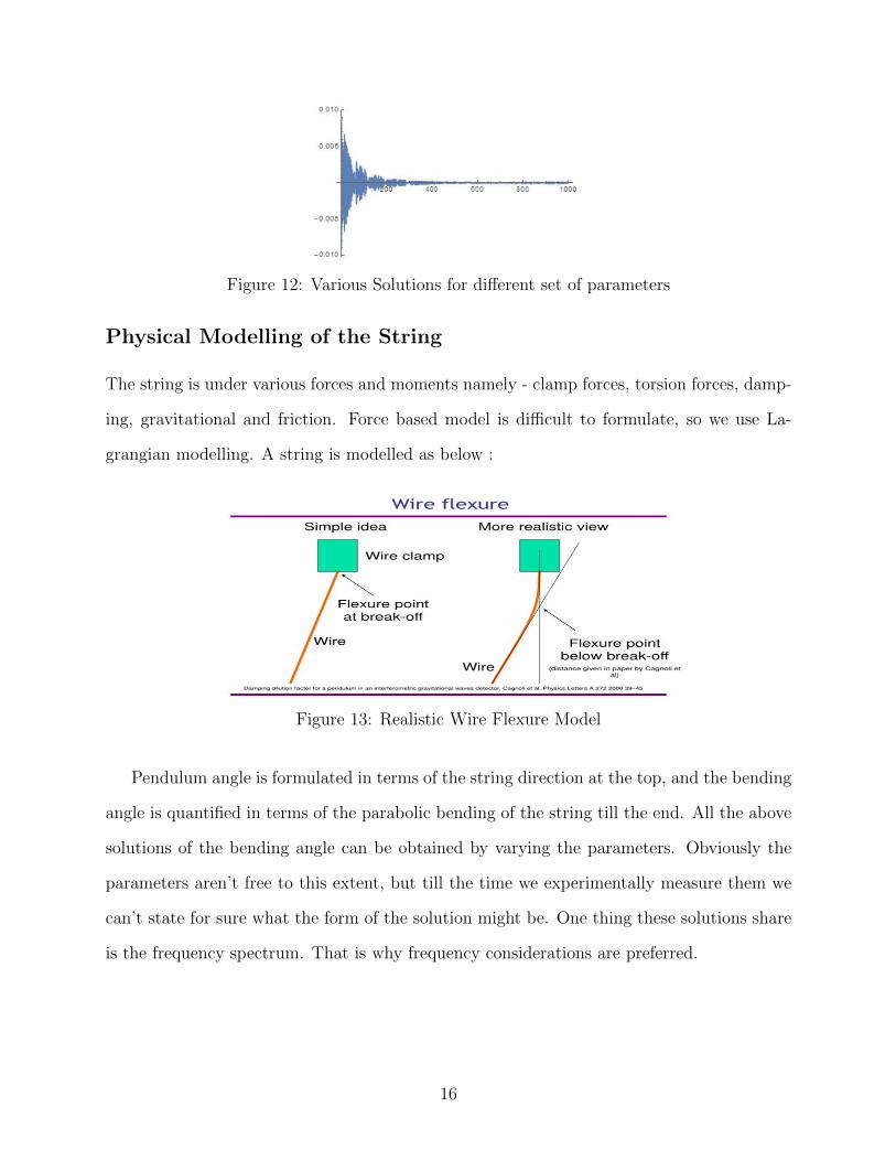
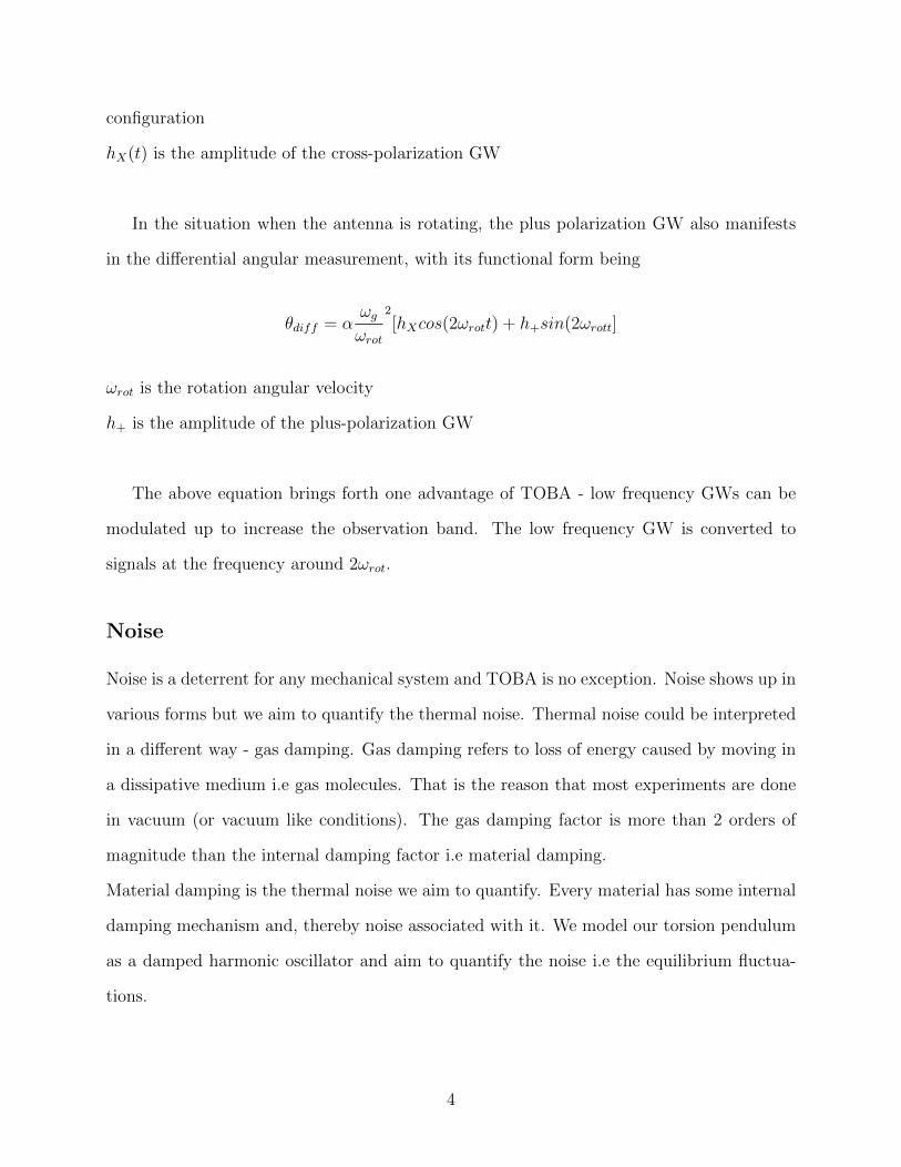
Figure 12: Various Solutions for different set of parameters

Physical Modelling of the String

The string is under various forces and moments namely - clamp forces, torsion forces, damp-

ing, gravitational and friction. Force based model is difficult to formulate, so we use La-

grangian modelling. A string is modelled as below :

Figure 13: Realistic Wire Flexure Model

Pendulum angle is formulated in terms of the string direction at the top, and the bending

angle is quantified in terms of the parabolic bending of the string till the end. All the above

solutions of the bending angle can be obtained by varying the parameters. Obviously the

parameters aren’t free to this extent, but till the time we experimentally measure them we

can’t state for sure what the form of the solution might be. One thing these solutions share

is the frequency spectrum. That is why frequency considerations are preferred.

16

Acknowledgment

I would like to thank my supervisor, Associate Professor Ando Masaki, and the fellow stu-

dents in the research laboratory for taking their time in helping me with this project. I would

like to specially thank Mr Ooi Ching Pin, for putting up with my requests and questions

(in the midst of his master thesis submission) throughout the course of this project, and for

helping me get a sense of the world class Tokyo food scene.

I also thank the UTRIP office and University of Tokyo for providing accommodation, funding

and support for this project.

References

• Ooi Ching Pin, Master Thesis, Mechanical Loss of Crystal Fibres for Torsion Pendulum

Experiments, (2018)

• Ando et al, Torsion-bar Antenna for Low-frequency Gravitational-wave Observations,

Phys. Rev. Lett. 105, 161101 (2010)

• T. Shimoda et al, Seismic cross- coupling noise in torsion pendulums, Phys. Rev. D,

vol. 97, p. 104003, (2018)

• G.T Giles and R.C Ritter, Torsion balances, torsion pendulums, and related devices,

Review of Scientific Instruments 64, 283 (1993)

• Cagnoli et al, Damping dilution factor for a pendulum in an interferometric gravita-

tional waves detector, Physics Letters A 272 2000 3945 gravitational waves detector

17