Characterizing the Nanoscale Layers of Tomorrow’s Electronics :

An Application of Fourier Analysis

Chris Payne

In Collaboration With: Apurva Mehta & Matt Bibee

A Relevant Challenge

Moore’s Law demands smaller devicesEconomically smart

Compatible with current fabrication facilities

The electronics industry is increasingly focusing on thin film applications …

…but they need a way to characterize the layer structure of these devices on

the nanometer scale

Bearing in mind a single page is about 100,000 nanometers thick

~200nm

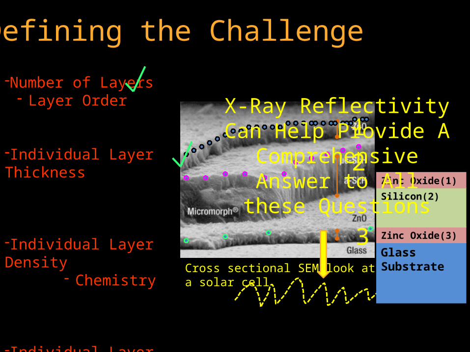
Defining the Challenge

-Number of Layers- Layer Order

-Individual Layer Thickness

-Individual Layer Density- Chemistry

-Individual Layer Roughness

12

3Glass SubstrateZinc Oxide(3)

Silicon(2)

Zinc Oxide(1)

Cross sectional SEM look at a solar cell

X-Ray Reflectivity Can Help Provide A

Comprehensive Answer to All these Questions

Our Tool : XRR

Reflectivity Detector

Substrate

Thin Top Layer

X-Ray Source

Θ

z

λ

The path length difference causes interference patterns to arise at the detector according to:

Reflectivity Detector

X-Ray Source

𝑃𝑎𝑡ℎ 𝐿𝑒𝑛𝑔𝑡ℎ 𝐷𝑖𝑓𝑓𝑒𝑟𝑒𝑛𝑐𝑒= 2𝑧𝑠𝑖𝑛(𝜃)𝜆

The path length distance, a function of Θ and Z, is embedding information in the interference pattern seen by the detector,

But what does this interference look like?

How this Interference appears in the Data

Θ

z

λ

The varying interference appears as

oscillations that span over

8 Orders of Magnitude!

0 1 2 3 4 5 6 7 8 9-9

-8

-7

-6

-5

-4

-3

-2

-1

0

theta

log(intensity)

𝑃𝑎𝑡ℎ 𝐿𝑒𝑛𝑔𝑡ℎ 𝐷𝑖𝑓𝑓𝑒𝑟𝑒𝑛𝑐𝑒= 2𝑧𝑠𝑖𝑛(𝜃)𝜆

The oscillations carry the information we want!

1. We first convert Θ to S which importantly gives the X – axis units of m-1

𝑠= 2sin(𝜃)𝜆 [𝑚−1]

2. The intensity can now be approximated (assuming no roughness) as

I

𝐼𝑛𝑡𝑒𝑛𝑠𝑖𝑡𝑦ሺ𝑆ሻ= 1𝑆4ቤ𝐹𝑇(𝑑𝜌ሺ𝑧ሻ𝑑𝑧 )ቤ2

Extracting Oscillations Mathematically

Layer 2

SubstrateLayer 1

Z

Derivate of Density

Depth Along Z

Θ

Z

𝐼𝑛𝑡𝑒𝑛𝑠𝑖𝑡𝑦ሺ𝑆ሻ≈ 𝐹𝑎𝑙𝑙𝑜𝑓𝑓ȁ+𝐹𝑇(𝑇ℎ𝑖𝑐𝑘𝑛𝑒𝑠𝑠 𝐺𝑟𝑎𝑑𝑖𝑒𝑛𝑡)ȁ+2

𝐼𝑛𝑡𝑒𝑛𝑠𝑖𝑡𝑦ሺ𝑆ሻ≈ 𝐹𝑎𝑙𝑙𝑜𝑓𝑓ȁ+𝐹𝑇(𝑇ℎ𝑖𝑐𝑘𝑛𝑒𝑠𝑠 𝐺𝑟𝑎𝑑∗𝑇ℎ𝑖𝑐𝑘𝑛𝑒𝑠𝑠 𝐺𝑟𝑎𝑑)ȁ+

Extracting Oscillations Mathematically

3. Lastly, lets cut out the Falloff term and free the thickness information from the FT, by taking the inverse FT

2N Algorithm(Because the falloff isn’t as simple as s4 )

Inverse Fourier Transform

𝐼𝑛𝑡𝑒𝑛𝑠𝑖𝑡𝑦ሺ𝑆ሻ≈ 𝐹𝑎𝑙𝑙𝑜𝑓𝑓ȁ+𝐹𝑇(𝑇ℎ𝑖𝑐𝑘𝑛𝑒𝑠𝑠 𝐺𝑟𝑎𝑑𝑖𝑒𝑛𝑡)ȁ+2 𝐼𝑛𝑡𝑒𝑛𝑠𝑖𝑡𝑦ሺ𝑆ሻ≈ 𝐹𝑎𝑙𝑙𝑜𝑓𝑓ȁ+𝐹𝑇(𝑇ℎ𝑖𝑐𝑘𝑛𝑒𝑠𝑠 𝐺𝑟𝑎𝑑∗𝑇ℎ𝑖𝑐𝑘𝑛𝑒𝑠𝑠 𝐺𝑟𝑎𝑑)ȁ+

Applying the Math to Simulated Data

Substrate

Layer 1

Layer 2

2 nm

20 nm

Using a simulation program, I generate raw intensity data for two layers on a substrate

Applying the Math to Simulated Data

Then I convert to s: 𝑠= 2sin(𝜃)𝜆 [𝑚−1]

Applying the Math to Simulated Data

Calculate local average point by point using 2N Method

1.7 1.8 1.9 2 2.1 2.2 2.3 2.4 2.5 2.6 2.7

-6.2

-6.1

-6

-5.9

-5.8

-5.7

-5.6

-5.5

-5.4

-5.3

-5.2

theta

log(intensity)

S [Gm-1]

Applying the Math to Simulated Data

Remove the falloff: 𝐼𝑛𝑡𝑒𝑛𝑠𝑖𝑡𝑦ሺ𝑆ሻ= 𝐹𝑎𝑙𝑙𝑜𝑓𝑓ȁ+𝐹𝑇(𝑇ℎ𝑖𝑐𝑘𝑛𝑒𝑠𝑠∗𝑇ℎ𝑖𝑐𝑘𝑛𝑒𝑠𝑠)ȁ+

S [Gm-1]

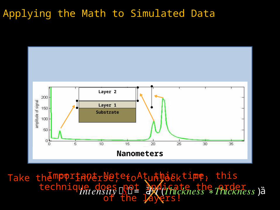
Applying the Math to Simulated Data

Take the FT inverse, to ‘unlock’ FT: 𝐼𝑛𝑡𝑒𝑛𝑠𝑖𝑡𝑦ሺ𝑆ሻ= ȁ+𝐹𝑇(𝑇ℎ𝑖𝑐𝑘𝑛𝑒𝑠𝑠∗𝑇ℎ𝑖𝑐𝑘𝑛𝑒𝑠𝑠)ȁ+

Substrate

Layer 1

Layer 2

Important Note: At this time, this technique does not indicate the order of the layers!

Nanometers

Applying this Process to Real Data

Original Sample Cleaned Sample

???Silicon Oxide

SiC Substrate

???Silicon Oxide

SiC Substrate

Thank You For Your Time

Especially Apurva Mehta & Matt Bibee