Comput. Methods Appl. Mech. Engrg. 199 (2010) 439–449

Contents lists available at ScienceDirect

Comput. Methods Appl. Mech. Engrg.

journal homepage: www.elsevier .com/locate /cma

A three-dimensional numerical model for incompressible two-phase flowof a granular bed submitted to a laminar shearing flow

Julien Chauchat *, Marc MédaleIUSTI CNRS UMR 6595, Polytech’Marseille, Aix-Marseille Université (U1), 5 rue Enrico Fermi, 13453 Marseille cedex 13, France

a r t i c l e i n f o a b s t r a c t

Article history:Received 14 April 2009Received in revised form 10 July 2009Accepted 24 July 2009Available online 3 August 2009

Keywords:Two-phase flow modelFluid–particle couplingVisco-plastic flowRegularisation techniqueQuadratic finite element

0045-7825/$ - see front matter � 2009 Elsevier B.V. Adoi:10.1016/j.cma.2009.07.007

* Corresponding author.E-mail address: julien.chauchat@polytech.univ-mr

A numerical model for the simulation of incompressible two-phase flows of a flat granular bed submittedto a laminar shearing flow is presented, considering a two-fluid model and a mixed-fluid one. The gov-erning equations are discretized by a finite element method and a penalisation method is introducedto cope with the incompressibility constraint. A regularisation technique is used to deal with thevisco-plastic behaviour of the granular phase. Validations are carried out on three flow test cases: a Bing-ham fluid between two infinite parallel planes, a Bingham fluid in a square lid-driven cavity and a New-tonian fluid over a granular bed in a two-dimensional configuration, for which we compare our numericalresults with existing analytical or numerical results. The accuracy and efficiency of the numerical modelshave been compared for the two formulations of the two-phase flow model. It turns out that the two-fluidmodel requires ten times more CPU time than the mixed-fluid one for a comparable accuracy, which canbe achieved provided one takes a smaller regularisation parameter in the latter model. Finally, three-dimensional computations are presented for the flow of a Newtonian fluid over a granular bed in a squareand circular cross-section ducts.

� 2009 Elsevier B.V. All rights reserved.

1. Introduction

Particles transport occurs in a variety of environmental andindustrial flows such as sediment transport in rivers or at coasts,hydrate formation in pipelines (oil production) or granular trans-port in food or pharmaceutical industries. There are mainly twomodes for particles to be transported by a flow: suspended-loador bed-load. Suspended-load is the part of the load where particlesare carried without contact with the bed. On the other way, bed-load is the part of the load that is carried with intermittent contactwith the bed, by rolling, sliding and bouncing [15]. In this paper,we focus only on the bed-load transport and more precisely in lam-inar flow conditions.

The bed-load transport is by nature a two-phase problem(fluid–particles). The particles of the bed are moving dependingon the value of the shear stress exerted by the fluid, the shearstress being usually made dimensionless by the apparent weightof a single particle the so-called Shields number h [31]. If theShields number based on the fluid bed shear stress is lower thana critical value hc the particle flux is zero otherwise it evolves asa function of h and hc [13,4,32,11,28]. The bed-load is usually mod-elled as a two-layer problem: a pure fluid layer at the top and afluid–particles mixture layer at the bottom, the two layers being

ll rights reserved.

s.fr (J. Chauchat).

separated by the bed upper surface. The fluid motion in the upperlayer is solved assuming weak interactions between the two layers.From this calculation the fluid bed shear stress is known and theparticle flux in the lower layer is deduced from an algebraic rela-tionship. A different approach for the bed-load has been proposedby Ouriemi et al. [26]. The authors have proposed some closures ofthe two-phase model which are appropriate to a situation in whichthe sediment can be considered as a mobile granular mediumwhere the particles are in contact: the interphase force is thenDarcy drag and buoyancy, the fluid phase stress is of Newtonianform, and the particle phase stress is described by a granular rhe-ology (Coulomb friction).

The granular rheology shares some properties with visco-plasticrheology, in particular it exhibits a threshold of motion due to thefriction between grains. The archetype model for visco-plasticmaterial is the Bingham model [9]. It is possible to identify theCoulomb friction model for the granular media with the Binghammodel in which the fluid viscosity vanishes. The simulation ofBingham fluid flows have been the subject of many papers in theliterature (see [12] for a recent review). There are mainly two ap-proaches to deal with the yield stress in the Bingham model: theAugmented Lagrangian technique [14,17] and the regularisationtechnique [8,29,16]. In the Augmented Lagrangian technique, thediscontinuity in the Bingham constitutive relationship is treatedby introducing a new primal variable and a Lagrange multiplierthat enforces it to be equal to the strain rate tensor. This method

440 J. Chauchat, M. Médale / Comput. Methods Appl. Mech. Engrg. 199 (2010) 439–449

is particularly accurate to capture and predict the yielded regionsof the flow. In the regularisation approach, the Bingham viscosityis ‘‘regularised” by adding a small quantity to the magnitude ofthe rate-of-strain tensor in the denominator. The solid regime is re-placed by a very viscous one. But the cost overrun for the Aug-mented Lagrangian Methods compared with regularization one isobvious in terms of memory due to the introduction of an addi-tional tensor variable (the ‘‘true” strain rate), whereas in terms ofCPU time the comparison is not known a priori. Actually, the regu-larized problem is equivalent to the flow of a shear thinning mate-rial that induces additional non-linearity in the equations. Thecomputation of which can significantly increase the CPU timeand do not allow to conclude on the most efficient method. How-ever, let us mention that the implementation of the regularizationmethod is easier than the Augmented Lagrangian one. Thereforewe choose the regularisation technique to deal with the yieldstress in our two-phase flow model. This method is advantageousfor its simplicity but one must be careful of the induced creepingflow in the yielded regions that arises when using regularisation.

In this paper we present a three-dimensional finite elementmethod (FEM) model of the two-phase incompressible flow modelfor bed-load transport presented by Ouriemi et al. [26]. Our firstconcern is to propose a numerical model able to predict accuratelythe bed-load transport in laminar shearing flows. It is restricted tothe cases where the granular bed does not change its shape in thecourse of time, consequently ripples and dunes formation are be-yond the scope of this paper. We have considered two formulationsof the two-phase model. In the two-fluid model the unknowns arethe velocities and pressure in each phase (fluid and particles)whereas in the mixed-fluid model the fluid–particles mixture isonly considered assuming that fluid and particles have the samevelocity. The computational efficiency of the numerical modelsassociated with both formulations is investigated in terms of accu-racy, CPU time and memory usage. The two-phase flow modelequations and the numerical modelling are presented in Section 2.Section 3 is devoted to the validation of the model by comparisonwith analytical solutions or published numerical results. Firstly, wehave validated the numerical model for Bingham fluid flows ontwo test cases. We have compared the numerical model with ananalytical solution for the flow of a Bingham fluid between twoinfinite parallel planes. We have also compared our model withthe numerical results of Mitsoulis and Zisis [24] for the flow of aBingham fluid in a square lid-driven cavity. Then we have validatedthe numerical model with the analytical solution presented byOuriemi et al. [26] for the flow of a Newtonian fluid over a granularbed in a two-dimensional configuration. After the validation, wepresent in Section 4 the application of the two-phase model to sim-ulate the bed-load transport in three-dimensional configurations, asquare cross-section and a circular cross-section ducts. Finally, wegive concluding remarks in Section 5.

2. The two-phase flow model

Following Ouriemi et al. [26], we present here the formulationof the two-phase flow model for bed-load transport in laminarshearing flows.

2.1. Mathematical formulation

2.1.1. Governing equationsGiven a cartesian coordinate system ðO; x; y; zÞ where x repre-

sents the stream-wise direction, y the lateral direction and z thevertical upward direction, the velocity vector of the k phase andits cartesian components are respectively denoted by

uk!¼ ðuk;vk;wkÞ. k is taken to be f for the fluid phase and p for

the particulate one. We start from Jackson’s equations [21] to getthe set of governing equations for the two-phase problem.

For the fluid phase, the continuity equation reads:

@�@tþr � �uf

!� �¼ 0; ð1Þ

where � designates the volume fraction of the fluid phase. The par-ticulate phase continuity equation has the same form:

@/@tþr � / up

!� �¼ 0; ð2Þ

where / is the particulate phase volume fraction. The global volumeconservation imposes /þ � ¼ 1.

The momentum equations for the fluid and particulate phasesare respectively:

qf@�uf

!

@tþr � �uf

!�uf!� �2

435 ¼ r � ðrf Þ � n~f þ �qf~g; ð3Þ

qp@/ up

!

@tþr � / up

!�up!� �2

435 ¼ r � ðrpÞ þ n~f þ /qp~g; ð4Þ

where rf and rp represent the stress tensor associated with thefluid and particulate phases respectively. n~f represents the averageforce exerted by the fluid on the particles and~g is the gravity accel-eration vector.

The set of partial differential Eqs. (1)–(4) introduces more un-knowns than the number of equations then closure relationshipsare needed to solve the problem. These relations are of two types:fluid–particle interactions and stress tensor expressions.

2.1.2. Closures2.1.2.1. Interaction term. Following Jackson [21] the average forceexerted by the fluid on the particles can be decomposed in twocontributions. The first one corresponds to the generalized buoy-ancy force and the second one gathers all the remainingcontributions.

n~f ¼ /r � ðrf Þ þ n f 1!

ð5Þ

For a viscous fluid flow in a porous media, the remaining contribu-tions reduce to the viscous drag force due to the relative motion be-tween phases. Using the Darcy law, the term n f 1

!can be written:

n f 1!¼ g

�2

Kuf!�up!� �

; ð6Þ

where g is the dynamic viscosity of the pure fluid. The coefficient ofpermeability is empirically linked to � and the particle diameter dby the Carman–Kozeny relationship:

K ¼ �3d2

kCKð1� �Þ2ð7Þ

A typical value for kCK � 180 is proposed by Happel and Brenner[20] and Goharzadeh et al. [18].

2.1.2.2. Stress tensors. The fluid phase has been assumed to be aNewtonian viscous liquid in which the Einstein dilute viscosity for-mula has been chosen to be applied to the concentrated situation:

rf ¼ �pf I þ sf ¼ �pf I þ ge rum!þðr um

!ÞT

� �; ð8Þ

where ge ¼ gð1þ 5/=2Þ is the effective viscosity of the mixture and

um!¼ �uf

!þ/ up

!is the velocity of the mixture.

Fig. 1. Sketch of domain definition for the fluid–particle problem.

J. Chauchat, M. Médale / Comput. Methods Appl. Mech. Engrg. 199 (2010) 439–449 441

The particle phase has been assumed to be described by Cou-lomb solid friction in which the extra stress is proportional tothe particle pressure.

rp ¼ �ppI þ sp ð9Þ

In the frame of the three-dimensional model we express the Cou-lomb friction model in tensorial form following the idea of Jopet al. [22]:

sp ¼ gpðk _cpk; ppÞ _cp; ð10Þ

with

gpðk _cpk;ppÞ ¼ lpp

k _cpk; ð11Þ

where the rate-of-strain tensor _cp is defined as _cp ¼ rup!þðrup

!ÞT

and its magnitude is given by the square root of its second invariant

k _cpk ¼ffiffiffiffiffiffiffiffiffiffiffiffiffiffiffiffi12 Trð _c2Þ

q. We emphasise that this expression in the one-

dimensional case reduces to the classical Coulomb expression:sp

xz ¼ lpp.

2.1.3. Dimensionless equationsIn the preceding subsections we have presented the ingredients

of the two-phase model for bed-load transport, we summarise herethe model equations to be solved. We consider two formulations ofthe model. The first one, called the two-fluid model, is based on thesolution of mass and momentum conservation equations for eachphase (12). The second one, called the mixed-fluid model, is basedon the solution of mass and momentum equations for the mixture(13) (i.e. a single effective phase is considered). In this latter formu-lation, the mass and momentum equations are simply obtained bysumming the corresponding equations over each phase (fluid andparticles).

In the following, we assume that the volume fractions are con-stant in space and time meaning that the interface between thefluid–particle mixture and the pure fluid region is fixed and no dila-tation occurs. This assumption implies that fluid and particulatephase as well as the mixture are incompressible. We also expressthe equations for the fluid phase in terms of the mixture velocity.

Following Ouriemi et al. [26] we make all the values dimension-less by scaling the length by H, the height of the flow, and the stressesby DqgH, and therefore the time by g=DqgH where Dq ¼ qp � qf .Using these scales one obtains the following dimensionless equa-tions for the two formulations of the two-phase model.

2.1.3.1. Two-fluid model.

r� um!

� �¼0

r� up!

� �¼0

GaH3

d3Dum!

Dt ¼�rpf þr� geg rum

!þrum

!T

� �� ��H2

K um!�up!

� �þ qf~g

Dqk~gk

Ga H3

d3 Rq/Dup!

Dt ¼�rppþr� gp

g rup!þrup

!T

� �� ��/rpf

þ/r� geg rum

!þrum

!T

� �� �þð1�/ÞH2

K um!�up!

� �þ /~gk~gk

8>>>>>>>>>>>>>>>>><>>>>>>>>>>>>>>>>>:

ð12Þ

In these equations, Rq ¼ qf =qp represents the density ratio andGa ¼ d3qf Dqg=g2 is the Galileo number where d is the particlediameter. The Galileo number is a Reynolds number based on thesettling velocity of particles.

2.1.3.2. Mixed-fluid model.

r � um!

� �¼ 0

Ga H3

d3 ð1þ RqÞ D um!

Dt ¼ �rpf �rpp þ qm~gDqk~gk

þr � geg rum

!þrum

!T

� �� �þr � gp

g ðrum!þrum

!TÞ

� �

8>>>>>><>>>>>>:

ð13Þ

2.2. Numerical model

The finite element method (FEM) leads to the discretisation ofthe variational formulation of Eq. (12) for the two-fluid modeland on Eq. (13) for the mixed-fluid model.

2.2.1. Weak formulations2.2.1.1. Weak formulation for the two-fluid model. Let us define thephysical domains associated with the pure fluid and the fluid–par-ticles mixture by Xf and Xp respectively and their respectiveboundaries by Cf and Cp (see Fig. 1). From the previous systemof partial differential equations (12) one obtains the followingweak formulation of the momentum equations for the two-fluidformulation [10,30]:

Find umh

!2 Uh and pf 2 Qh satisfying (14) and (15) and find

uph

!2 Uh and pp 2 Qh satisfying (16) and (17) 8 du

!2Vh and

8 dp 2 Qh where

Uh ¼ f~u 2 H1ðXÞj~u ¼ ~uDirichlet on @XDirichletg;Qh ¼ fdp 2 L2ðXÞg;

Vh ¼ du!2 H1

0ðXÞj du!¼~0 on@XDirichlet

� �:

0 ¼Z

Xf [Xp

dp � rumh

!dX; ð14Þ

0 ¼ �Z

Xf[Xp

GaH3

d3 du!�D um

h

!

DtdX�

ZXf [Xp

du!�rpf

hdXþZ

Xp

H2

K

� du!� up

h

!�um

h

!� �dX�

ZXf [Xp

ge

gr du!þrdu

!T

� �

� rumh

!þrum

h

!T

� �dXþ

ZXf[Xp

qf

Dqdu!�~gk~gk dX; ð15Þ

0 ¼Z

Xp

dp � r uph

!dX; ð16Þ

442 J. Chauchat, M. Médale / Comput. Methods Appl. Mech. Engrg. 199 (2010) 439–449

0 ¼ �Z

Xp

GaH3

d3 Rq/ du!�D up

h

!

DtdX�

ZXp

du!�ðrpp

h � /rpfhÞdX

�Z

Xp

ð1� /ÞH2

Kdu!� up

h

!�um

h

!� �dX

�Z

Xp

gp r du!þrdu

!T

� �rup

h

!þrup

h

!T

� �dX

þZ

Cp

gp du!�ðr up

h

!þrup

h

!TÞ �~ndC

�Z

Xp

/ge

gðr du

!þrdu

!TÞðrum

h

!þrum

h

!TÞdX

þZ

Cp

/ge

gdu!�ðrum

h

!þrum

h

!TÞ �~ndCþ

ZXp

/ du!�~gk~gk dX� ð17Þ

2.2.1.2. Weak formulation for the mixed-fluid model. For the mixed-fluid model, the weak formulation is given by:

Find umh

!2 Uh and pf and pp 2 Qh satisfying (18) and (19)

8 du!2Vh and 8 dp 2 Qh where

Uh ¼ f~u 2 H1ðXÞj~u ¼~uDirichlet on @XDirichletg;Qh ¼ fdp 2 L2ðXÞg;

Vh ¼ du!2 H1

0ðXÞj du!¼~0 on @XDirichlet

� �;

0 ¼Z

Xf [Xp

dp � rumh dX; ð18Þ

0 ¼Z

Xf [Xp

GaH3

d3 ð1þ RqÞ du!�Dum

h

DtdX�

ZXf[Xp

du!�ðrpp

h þrpfhÞdX

�Z

Xf [Xp

gp þ ge

gr du!þrdu

!T

� �rum

h

!þrum

h

!T

� �dX

þZ

Xf [Xp

qm

Dqdu!�~gk~gk dX: ð19Þ

2.2.2. Algorithms associated with the two formulationsThe first algorithm dealing with the two-fluid formulation is

based on the solution of the system (14)–(17) in a weakly coupledway. For each Newton–Raphson iteration we solve for the fluidmomentum Eq. (15) whereas the particulate phase velocity is ta-ken at its previous iteration value. From the value of the mixturevelocity obtained at this stage the particulate phase velocity iscomputed by solving Eq. (17). On the other hand the algorithm de-voted to the mixed-fluid formulation is based on the solution of thesystem (18) and (19).

The non-linearities in the governing equations are solved by aNewton–Raphson algorithm by taking the first variation of the var-iational formulations (15)–(17), (19). Only the advective terms andthe particle stress term (visco-plastic) induce a contribution in thefirst variation of the variational formulations.

2.3. Regularisation technique

The stress tensor for the particulate phase (10) reveals the pres-ence of a yield stress that depends on the granular pressure. Themixed-fluid model (13) can be identified as a Bingham fluid inwhich the yield stress vary linearly with the granular pressure. Thisremark allows us to use some well-known methods derived forBingham flows to deal with the visco-plastic behaviour of thefluid–particle mixture.

As with a Bingham model, the particulate viscosity divergeswhen the shear rate tends toward zero, rising evident numericalproblems. The idea of a regularisation technique from a mathemat-

ical point of view is to smooth the divergence of the viscosity func-tion. The consequence on the computational behaviour of the yieldstress fluid results in a very viscous fluid at zero rate of strain in-stead of a pure rigid body behaviour. One of the easiest solutionsto regularise the viscosity is the following [16]:

gð _cÞ ¼ lþ s0

k _ck þ k;

where k is the regularisation parameter ðk� 1Þ and s0 is the yieldstress. We have chosen this expression in our implementation ofthe numerical model. A review of regularisation technique can befound in Frigaard and Nouar[16].

2.4. Implementation

In our implementation, we use piecewise quadratic polynomialapproximation for the velocity and piecewise linear discontinuousapproximation for the pressure. In the computations, we have em-ployed a 27-nodes hexahedra element (H27) for the velocities. Theincompressibility constraint is solved by a penalisation method.The code is developed with the PETSc library [6,5,7] which pro-vides several parallel iterative and direct solvers.

As we use a penalisation method to cope with the incompress-ibility constraint, all the algebraic systems have been solved by theMUMPS direct solver [2,1,3] with a penalty parameter set to 109 forall the simulations presented in this paper.

3. Validations

In this section we address a twofold goal for the validation ofour numerical model. The first one concerns the implementationof visco-plastic flow using a regularisation technique (Section 3.1)and the second one deals with the implementation of the two for-mulations associated with the two-fluid model and the mixed-fluidone (Section 3.2). In each case we discuss the accuracy and numer-ical efficiency of the implemented numerical model.

3.1. Test cases for Bingham fluid flows

We have begun with test cases on Bingham fluid flows becauseof the close link that exists between the Coulomb friction for theparticulate phase (10) and the Bingham fluid model. These twomodels exhibit the presence of a yield stress. This is particularlyimportant to validate the implementation of the regularisationon ‘‘well-known” configurations (Bingham fluid flows) in order toavoid questions on it when performing two-phase flows simula-tions. We have done two test cases. The first one is the flow of aBingham fluid between two infinite parallel planes. The secondone is the flow of a Bingham fluid in a square lid-driven cavity.

3.1.1. Flow of a Bingham fluid between two infinite planeIn this first test case we study the flow of a Bingham fluid be-

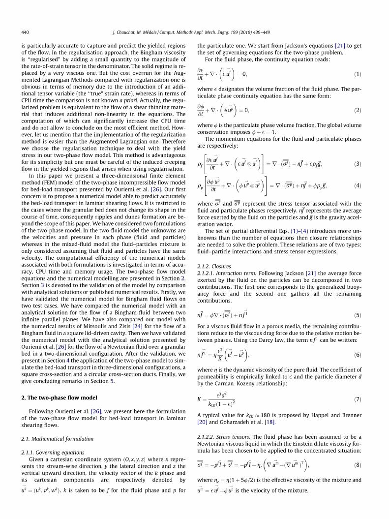
tween two infinite parallel planes. This is a 2D problem wherethe longitudinal velocity component only depends on the verticalcoordinate. This simple problem is particularly interesting for thevalidation since it possesses an analytical solution for the longitu-dinal velocity (See [19, pp. 219–220]). Fig. 2 shows the sketch ofthe problem and boundary conditions. The simulation are per-formed using a regularisation method with a regularisation param-eter k ¼ 10�4s�1 and the Bingham number (Bn) is equal to 10.

Fig. 3a shows the longitudinal velocity profiles for the numeri-cal solution and the analytical one. In order to study the spatialconvergence of the numerical model we have considered fivemeshes. The ratio of the mesh size in the three directions havebeen kept constant Dx=Dz ¼ Dx=Dy ¼ 10 to avoid errors induced

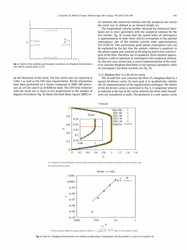
Fig. 2. Sketch of the problem and boundary conditions of a Bingham fluid betweentwo infinite parallel plane in 2D.

J. Chauchat, M. Médale / Comput. Methods Appl. Mech. Engrg. 199 (2010) 439–449 443

by the distortion of the mesh. The five mesh sizes are reported inTable 1 as well as the CPU time requirements. All the simulationshave been performed on a cluster composed of AMD 280 proces-sors at 2.4 GHz and 8 Go of RAM by node. The CPU time evolutionwith the mesh size is more or less proportional to the number ofdegrees of freedom. Fig. 3b shows the Root Mean Square (RMS) er-

Fig. 3. Flow of a Bingham fluid between two infinite parallel pla

ror between the numerical solution and the analytical one versusthe mesh size (h, defined as an element height Dz).

The longitudinal velocity profiles obtained by numerical simu-lation are in close agreement with the analytical solution for thefive meshes. Fig. 3b reveals that the spatial order of convergenceis approximately of order three which corresponds to the optimalconvergence rate of the method (second order approximation)[25,10,30,33]. This particularly good spatial convergence rate canbe explained by the fact that the analytic solution is quadratic inthe plastic region and constant in the plug located in the central re-gion of the flow. Therefore our tri-quadratic finite element approx-imation is able to represent at convergence this analytical solution.So, this test case reveals that a correct implementation of the mod-el to simulate Bingham fluid flows as the optimal asymptotic orderof convergence has been reached, see Fig. 3b.

3.1.2. Bingham flow in a lid-driven cavityThe second test case concerns the flow of a Bingham fluid in a

square lid-driven cavity. Its main goal is to qualitatively validatethe 3D implementation of the regularisation technique. The sketchof the lid-driven cavity is presented in Fig. 4. A tangential velocityis imposed at the top of the cavity whereas the three other bound-aries are considered as walls. The geometry is a unit square cavity

ne: longitudinal velocity profiles (a) and error analysis (b).

Table 1Mesh definition and CPU time per iteration.

Mesh definition (NX � NY � NZ) 3 � 1 � 10 6 � 1 � 20 12 � 1 � 40 24 � 1 � 80 48 � 1 � 160

Degrees of freedom 1323 4797 18,225 71,001 280,233CPU time (s/it. on 8 proc.) 0.67 1.88 6.98 27.79 116.74

444 J. Chauchat, M. Médale / Comput. Methods Appl. Mech. Engrg. 199 (2010) 439–449

and the velocity at the top is also chosen to be unity. This test casehas been extensively studied and a great amount of literature onvisco-plastic flows exists concerning this problem [24,23,12]. Wehave chosen the Mitsoulis and Zisis [24] results as reference whoalso used a FEM model and a regularisation technique to deal withthe yield stress. In the following simulations we have neglectedinertial effects (i.e. Re = 0). The dimensionless number controllingthe flow is the Bingham number ðBn ¼ s0H=gUÞ where s0 is theyield stress.

The mesh is composed with 60 � 1 � 60 quadratic elements(H27). The regularisation parameter is fixed to k ¼ 10�4 s�1. Thisvalue is equivalent to the one chosen by Mitsoulis and Zisis [24]but the regularisation technique is different. Mitsoulis and Zisis[24] used the Papanastasiou [29] regularisation whereas we haveused the simple regularisation (Cf. 2.3). In the simulations theBingham number has been considered in the range [0–20] to vali-date our model.

Fig. 5 shows the velocity fields in the cavity for various Binghamnumber (Bn = 0, 2 and 20). We observe that a rigid region appearsat the bottom of the cavity as the Bingham number is increased.Also the velocity decreases as well as the vortex intensity.

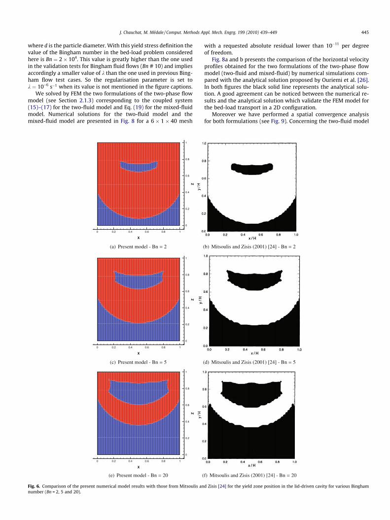
Fig. 6 shows the yield zone position in the lid-driven cavity forvarious Bingham number. We compare our results with the results

Fig. 4. Sketch of the lid-driven cavity.

Fig. 5. Velocity vector fields – Bin

from Mitsoulis and Zisis [24]. The position of the yield zone is de-fined as the position where the material flows (yields) i.e. wherethe magnitude of the stress tensor ksk exceeds the yield stresss0 ðkskP s0Þ. The results obtained are in good agreement withMitsoulis and Zisis [24] and validate the implementation of theBingham model in our FEM model.

As a conclusion on the two Bingham fluid flow test cases onecan notice that the regularisation technique implemented give sat-isfactorily accurate results for Bingham number in the range 0–20for a regularisation parameter k ¼ 10�4s�1. Moreover with thisnumerical parameter a third order (optimal) asymptotic conver-gence rate has been reached for our tri-quadratic finite elementapproximation.

3.2. Two-phase simulation of bed-load transport in 2D

In this subsection we present results on the flow of a Newtonianfluid over a granular bed. The aim of this subsection is first to val-idate quantitatively the two formulations of the two-phase flowmodel by comparison with the analytical solution of Ouriemiet al. [26] for the bed-load transport in laminar shearing flowsand secondly to assess computational efficiency of the numericalmodel associated with both formulations.

The sketch of the problem and boundary conditions are given inFig. 7. The lower half of the domain is filled with particles at/ ¼ 0:55 immersed in a fluid and the upper part is filled with purefluid ð/ ¼ 0Þ. Therefore in this problem the values of the dimen-sionless numbers are: Re ¼ 2� 10�2; Ga ¼ 11; Rq ¼ 0:4 andd=H ¼ 30. There are several choice for the definition of the Bing-ham number in the bed-load problem. Actually, in dense granularmedia the yield stress varies with the normal stress. Therefore onehas to choose a pertinent value of the yield stress. Here we choosethe yield stress corresponding to the first granular layer, this choiceis natural since the relevant length scale for the estimation of theyield stress is the height of the moving granular bed that is ofthe order of few grain diameters. Assuming a hydrostatic pressurefor the granular phase, it reads:

s0 ¼ lsDqgd;

gham varying from 0 to 20.

J. Chauchat, M. Médale / Comput. Methods Appl. Mech. Engrg. 199 (2010) 439–449 445

where d is the particle diameter. With this yield stress definition thevalue of the Bingham number in the bed-load problem consideredhere is Bn ¼ 2� 104. This value is greatly higher than the one usedin the validation tests for Bingham fluid flows (Bn # 10) and impliesaccordingly a smaller value of k than the one used in previous Bing-ham flow test cases. So the regularisation parameter is set tok ¼ 10�6 s�1 when its value is not mentioned in the figure captions.

We solved by FEM the two formulations of the two-phase flowmodel (see Section 2.1.3) corresponding to the coupled system(15)–(17) for the two-fluid model and Eq. (19) for the mixed-fluidmodel. Numerical solutions for the two-fluid model and themixed-fluid model are presented in Fig. 8 for a 6 � 1 � 40 mesh

Fig. 6. Comparison of the present numerical model results with those from Mitsoulis annumber (Bn = 2, 5 and 20).

with a requested absolute residual lower than 10�11 per degreeof freedom.

Fig. 8a and b presents the comparison of the horizontal velocityprofiles obtained for the two formulations of the two-phase flowmodel (two-fluid and mixed-fluid) by numerical simulations com-pared with the analytical solution proposed by Ouriemi et al. [26].In both figures the black solid line represents the analytical solu-tion. A good agreement can be noticed between the numerical re-sults and the analytical solution which validate the FEM model forthe bed-load transport in a 2D configuration.

Moreover we have performed a spatial convergence analysisfor both formulations (see Fig. 9). Concerning the two-fluid model

d Zisis [24] for the yield zone position in the lid-driven cavity for various Bingham

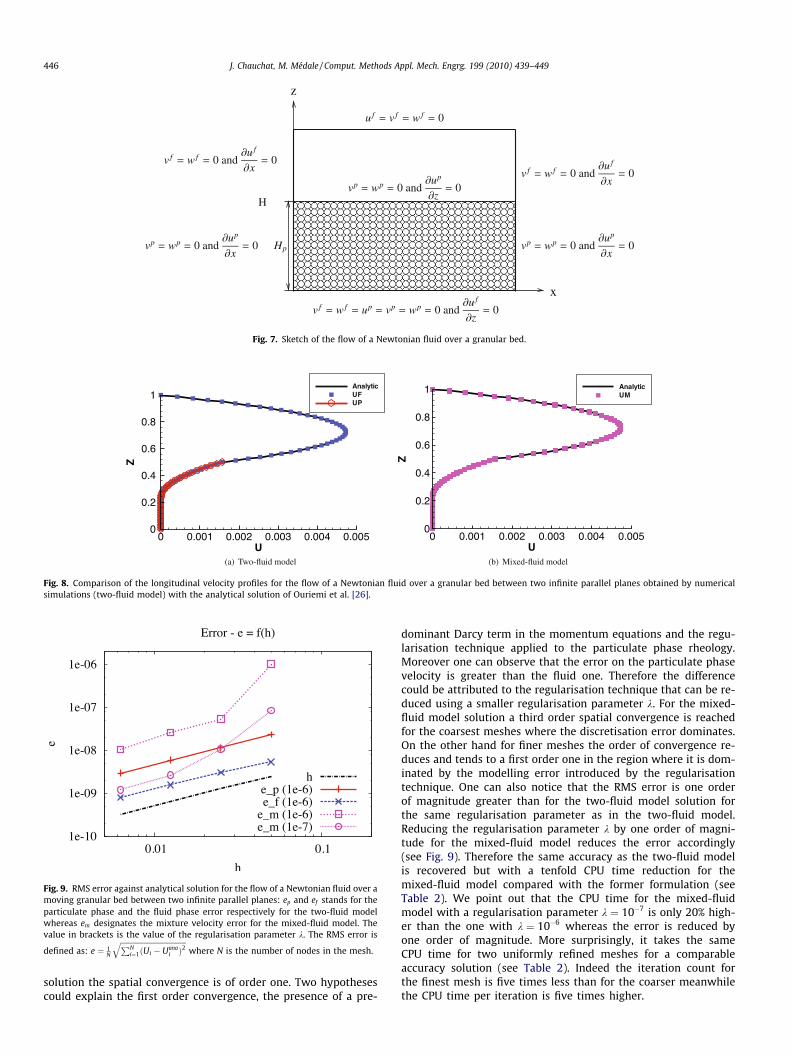
Fig. 7. Sketch of the flow of a Newtonian fluid over a granular bed.

Fig. 8. Comparison of the longitudinal velocity profiles for the flow of a Newtonian fluid over a granular bed between two infinite parallel planes obtained by numericalsimulations (two-fluid model) with the analytical solution of Ouriemi et al. [26].

Fig. 9. RMS error against analytical solution for the flow of a Newtonian fluid over amoving granular bed between two infinite parallel planes: ep and ef stands for theparticulate phase and the fluid phase error respectively for the two-fluid modelwhereas em designates the mixture velocity error for the mixed-fluid model. Thevalue in brackets is the value of the regularisation parameter k. The RMS error is

defined as: e ¼ 1N

ffiffiffiffiffiffiffiffiffiffiffiffiffiffiffiffiffiffiffiffiffiffiffiffiffiffiffiffiffiffiffiffiffiffiffiffiPNi¼1ðUi � Uana

i Þ2

qwhere N is the number of nodes in the mesh.

446 J. Chauchat, M. Médale / Comput. Methods Appl. Mech. Engrg. 199 (2010) 439–449

solution the spatial convergence is of order one. Two hypothesescould explain the first order convergence, the presence of a pre-

dominant Darcy term in the momentum equations and the regu-larisation technique applied to the particulate phase rheology.Moreover one can observe that the error on the particulate phasevelocity is greater than the fluid one. Therefore the differencecould be attributed to the regularisation technique that can be re-duced using a smaller regularisation parameter k. For the mixed-fluid model solution a third order spatial convergence is reachedfor the coarsest meshes where the discretisation error dominates.On the other hand for finer meshes the order of convergence re-duces and tends to a first order one in the region where it is dom-inated by the modelling error introduced by the regularisationtechnique. One can also notice that the RMS error is one orderof magnitude greater than for the two-fluid model solution forthe same regularisation parameter as in the two-fluid model.Reducing the regularisation parameter k by one order of magni-tude for the mixed-fluid model reduces the error accordingly(see Fig. 9). Therefore the same accuracy as the two-fluid modelis recovered but with a tenfold CPU time reduction for themixed-fluid model compared with the former formulation (seeTable 2). We point out that the CPU time for the mixed-fluidmodel with a regularisation parameter k ¼ 10�7 is only 20% high-er than the one with k ¼ 10�6 whereas the error is reduced byone order of magnitude. More surprisingly, it takes the sameCPU time for two uniformly refined meshes for a comparableaccuracy solution (see Table 2). Indeed the iteration count forthe finest mesh is five times less than for the coarser meanwhilethe CPU time per iteration is five times higher.

Table 2CPU time and number of iterations.

Mesh definition NX � NY � NZ 12 � 1 � 80 24 � 1 � 160

Two-fluid model DOFa 54450 212562

k ¼ 10�6 Niterb 1943 206

CPU time (s) 5682 5476

Mixed-fluid model DOF 36225 141561

k ¼ 10�6 Niter 269 54

CPU time (s) 438 473

k ¼ 10�7 Niter 253 75

CPU time (s) 453 589

a DOF: degrees of freedom.b Niter: number of iterations.

J. Chauchat, M. Médale / Comput. Methods Appl. Mech. Engrg. 199 (2010) 439–449 447

Consequently the two-fluid model is much more expensive (tentimes in CPU time) than the mixed-fluid one for a comparableaccuracy provided one takes a regularisation parameter sufficientlysmall (one order of magnitude smaller than in the two-fluid mod-el). But one should keep in mind that the mixed-fluid model isbased on the strong assumption of zero relative velocity between

Fig. 11. Mesh sensitivity of the velocity profiles obtained by numerical simulations6 � 40 � 80).

Fig. 10. Velocity profile obtained by numerical simulations with the mixed-fluidmodel for the square cross-section duct (6 � 20 � 40).

the fluid and particulate phases, which could be restrictive in ac-tual problems.

It turns out from the results obtained in this section that themodelling error associated with the implemented regularisationtechnique is connected to the regularisation parameter value k.Therefore in order to achieve computations with controlled accu-racy we suggest to link the value of the regularisation parameterto the Bingham number according to the following empirical rela-tionship: k ¼ min 10�4; 10�4

Bn

� �.

4. Two-phase simulation of bed-load transport in 3Dconfiguration

We have shown in the last section the convergence of the two-phase numerical model compared with analytical solution for atwo-dimensional configuration. We now apply the model tothree-dimensional configurations: a square and a circular cross-section ducts. As in the previous test case the values of the dimen-

with the mixed-fluid model for the square cross-section duct (6 � 20 � 40 and

Fig. 12. Velocity profile obtained by numerical simulations with the two-fluidmodel for the square cross-section duct (6 � 20 � 40). The fluid phase velocity is inblue and the particulate phase velocity is in red. An offset of 10�3 has been added tothe velocity of the particulate phase (up) to make it visible. (For interpretation ofthe references to color in this figure legend, the reader is referred to the web versionof this article.)

448 J. Chauchat, M. Médale / Comput. Methods Appl. Mech. Engrg. 199 (2010) 439–449

sionless numbers are: Re ¼ 2� 10�2; Ga ¼ 11; Rq ¼ 0:4; d=H ¼ 30and Bn ¼ 2� 104. However the characteristic length in the defini-tion of the dimensionless numbers is the side length for the squareduct whereas it is the diameter in the cylindrical one.

4.1. Square section duct

We have performed simulations for a square cross-section ductwith two meshes: 6 � 20 � 40 and 6 � 40 � 80 elements uniformlydistributed, only the half of the domain has been solved in thetransverse direction for obvious symmetry reasons. Fig. 10 showsthe velocity profile in a cross-section of the duct. The contour col-ors represent the x-velocity of the mixture ðumÞ. The horizontalthick solid line at z ¼ 0:5 represents the position of the granularbed. The fluid and the mixture are sheared in both z and y direc-tions inducing an increase in the friction compared with the two-dimensional case. Due to this shear increase the velocity is lowerthan in the two-dimensional case. In order to test the convergenceof the solution with respect to the mesh we present in Fig. 11 thecomparison of the velocity profiles on the plane of symmetry of theduct (y = 0) for the two meshes. The numerical solutions superim-pose themselves except in the neighbourhood of the yield zone

Fig. 13. Velocity profile obtained by numerical simulations with the mixed-fluidmodel for the circular cross-section duct (6 � 896).

Fig. 14. Mesh sensitivity of the velocity profiles obtained by numerical simulations wit

where the finest mesh better resolves the yield zone. Fig. 12 showsthe velocity profiles of the fluid phase velocity in blue and the par-ticulate phase velocity in red (an offset of 10�3 has been added tomake the particulate phase velocity visible) obtained with the two-fluid model for the square cross-section duct (6 � 20 � 40). Thisillustrates the good behaviour of the numerical model in thisthree-dimensional configuration.

4.2. Circular section duct

As for the square cross-section duct we have performed two sim-ulations on the circular cross-section duct. The mesh sizes are6 � 896 and 6 � 3596 quadratic elements in the x direction and inthe cross-section respectively. Fig. 13 shows the velocity profile ina cross-section of the duct (6 � 896). As for the square cross-section

h the mixed-fluid model for the square cross-section duct (6 � 896 and 6 � 3596).

Fig. 15. Velocity profile obtained by numerical simulations with the two-fluidmodel for the circular cross-section duct (6 � 896). The fluid phase velocity is inblue and the particulate phase velocity is in red. An offset of 10�3 has been added tothe velocity of the particulate phase (up) to make it visible. (For interpretation ofthe references to color in this figure legend, the reader is referred to the web versionof this article.)

J. Chauchat, M. Médale / Comput. Methods Appl. Mech. Engrg. 199 (2010) 439–449 449

duct, the thick solid line at z ¼ 0 represents the position of the gran-ular bed and the contour colors represent the mixture velocity ðumÞ.Here again the friction is increased in this geometry compared withthe two-dimensional configuration. We have compared the velocityprofiles on the vertical plane of symmetry to show the convergenceof the solution with respect to the mesh size (see Fig. 14). AgainFig. 15 illustrates the good behaviour of the numerical model forthree-dimensional flow configurations.

5. Concluding remarks

In conclusion, we have developed a numerical model to simu-late incompressible two-phase flow of a Newtonian fluid over agranular bed. The model is based on a penalisation method forincompressible flows and a regularisation technique for the vis-co-plastic behaviour of the granular phase. Validations have beencarried out on three test cases: the flow of a Bingham fluid betweentwo infinite parallel planes, the flow of a Bingham fluid in a squarelid-driven cavity and the flow of a Newtonian fluid over a granularbed. One can notice the very good agreement between the compu-tations and the existing analytical solutions [19,26] or numericalresults [24]. To get these results we have considered that the mod-elling error associated with the implemented regularisation tech-nique should be correlated to the regularisation parameter valuek according to the empirical relationship: k ¼ minð10�4;10�4=BnÞ.

Concerning the two-phase flow formulation of the bed-loadproblem we have shown that the mixed-fluid model is computa-tionally more efficient than the two-fluid one (roughly ten timesfaster and requires 20% less memory). Moreover, in order toachieve a comparable accuracy of the two models one has tochoose a regularisation parameter ten times smaller for themixed-fluid model than for the two-fluid one. But one should recallthat the mixed-fluid formulation is based on the strong assump-tion that the fluid–particles relative velocity is negligible whichcould limits its validity range to the cases of small particulate Rey-nolds number.

Finally we have performed three-dimensional numerical simu-lation of the bed-load transport in a square and a circular cross-section ducts illustrating the capability of the model to deal witharbitrary geometries where no analytical solution exists. Futuredevelopments will concern the implementation of a numericaltechnique to simulate the motion of the fluid–granular bed inter-face. Our final goal is to perform three-dimensional simulationsfor the formation of ripples and dunes that are observed in exper-iments [27].

Acknowledgements

We would like to thank P. Aussillous and É. Guazzelli for fruitfuldiscussions regarding the two-phase flow model and Y. Forterreand O. Pouliquen for discussions regarding the granular rheology.The authors also acknowledge Y. Jobic for technical support. Fund-ing from Agence Nationale de la Recherche (Project Dunes ANR-07-3_18-3892) is gratefully acknowledged.

References

[1] P.R. Amestoy, I.S. Duff, J. Koster, J.-Y. L’Excellent, A fully asynchronousmultifrontal solver using distributed dynamic scheduling, SIAM J. MatrixAnal. Appl. 23 (1) (2001) 15–41.

[2] P.R. Amestoy, I.S. Duff, J.-Y. L’Excellent, Multifrontal parallel distributedsymmetric and unsymmetric solvers, Comput. Methods Appl. Mech. Engrg.184 (2000) 501–520.

[3] P.R. Amestoy, A. Guermouche, J.-Y. L’Excellent, S. Pralet, Hybrid scheduling forthe parallel solution of linear systems, Parallel Comput. 32 (2) (2006) 136–156.

[4] R.A. Bagnold, The flow of cohesionless grains in fluids, Philos. Trans. R. Soc.Lond. 249 (1956) 235–297.

[5] S. Balay, K. Buschelman, V. Eijkhout, W.D. Gropp, D. Kaushik, M.G. Knepley, L.C.McInnes, B.F. Smith, H. Zhang, PETSc users manual, Tech. Rep. ANL-95/11 –Revision 2.1.5, Argonne National Laboratory, 2004.

[6] S. Balay, K. Buschelman, W.D. Gropp, D. Kaushik, M.G. Knepley, L.C. McInnes,B.F. Smith, H. Zhang, PETSc Web Page, 2001, <http://www.mcs.anl.gov/petsc>.

[7] S. Balay, W.D. Gropp, L.C. McInnes, B.F. Smith, Efficient management ofparallelism in object oriented numerical software libraries, in: E. Arge, A.M.Bruaset, H.P. Langtangen (Eds.), Modern Software Tools in ScientificComputing, Birkhäuser Press, 1997, pp. 163–202.

[8] M. Bercovier, M. Engelman, A finite-element method for incompressiblenon-Newtonian flows, J. Comput. Phys. 36 (3) (1980) 313–326. <http://www.sciencedirect.com/science/article/B6WHY-4DDR302-7K/1/a27540473088dcd2a4e158910bbbc4a4> .

[9] E.C. Bingham, Fluidity and Plasticity, McGraw Hill, New York, 1922.[10] G. Carey, J.T. Oden, Finite Elements, Fluids Mechanics, The Texas Finite

Element Series, vol. VI, Prentice Hall, Englewood Cliffs, NJ, 1986.[11] F. Charru, H. Mouilleron-Arnould, O. Eiff, Erosion and deposition of particles on

a bed sheared by a viscous flow, J. Fluid Mech. 519 (1) (2004) 55–80.[12] E.J. Dean, R. Glowinski, G. Guidoboni, On the numerical simulation of bingham

visco-plastic flow: old and new results, J. Non-Newtonian Fluid Mech. 142 (1–3) (2007) 36–62. <http://www.sciencedirect.com/science/article/B6TGV-4KV846H-1/2/7a6e1bcd0ee1a120c885591aae6cfc6a> .

[13] H.A. Einstein, The bed load function for sedimentation in open channel channelflows, Tech. Rep. 1026, US Department of Agriculture, 1950.

[14] M. Fortin, R. Glowinski, Augmented Lagrangians: Application to the NumericaSolution of Boundary Value Problems, North-Holland, Amsterdam, 1983.

[15] J. Fredsoe, R. Deigaard, Mechanics of Costal Sediment Transport, WorldScientific, 1992.

[16] I.A. Frigaard, C. Nouar, On the usage of viscosity regularisation methods forvisco-plastic fluid flow computation, J. Non-Newtonian Fluid Mech. 127 (1)(2005) 1–26. <http://www.sciencedirect.com/science/article/B6TGV-4G4XBV2-1/2/b071488697d73549ac617789b903a4c7> .

[17] R. Glowinsky, P. Le Tallec, Augmented Lagrangians and Operator-SplittingMethods in Nonlinear Mechanics, SIAM, Philadelphia, 1989.

[18] A. Goharzadeh, A. Khalili, B.B. Jorgensen, Transition layer thickness at a fluid–porous interface, Phys. Fluids 17 (5) (2005) 057102. <http://link.aip.org/link/?PHF/17/057102/1> .

[19] E. Guyon, J.-P. Hulin, L. Petit, Hydrodynamique Physique, EDP Sciences – CNRSEditions, Paris, 2001.

[20] J. Happel, H. Brenner, Low Reynolds Number Hydrodynamics, Martinus Nijhof,The Hague, 1973.

[21] R. Jackson, The Dynamics of Fluidized Particles, Cambridge University Press,Cambridge, 2000.

[22] P. Jop, Y. Forterre, O. Pouliquen, A constitutive law for dense granular flows,Nature 441 (2006) 727–730. <http://dx.doi.org/10.1038/nature04801> .

[23] F. Lalli, P.G. Esposito, R. Piscopia, R. Verzicco, Fluid–particle flow simulationby averaged continuous model, Comput. Fluids 34 (9) (2005) 1040–1061.<http://www.science-direct.com/science/article/B6V26-4F3FDV3-2/1/59e809336e8c43572b2595b43f3a0631> .

[24] E. Mitsoulis, T. Zisis, Flow of bingham plastics in a lid-driven square cavity, J.Non-Newtonian Fluid Mech. 101 (2001) 173–180.

[25] J.T. Oden, G. Carey, Finite Elements, Mathematical Aspects, The Texas FiniteElement Series, vol. IV, Prentice Hall, Englewood Cliffs, NJ, 1986.

[26] M. Ouriemi, P. Aussillous, E. Guazzelli, Sediment dynamics. Part 1: bed-loadtransport by laminar shearing flows, J. Fluid Mech. 636 (2009) 295–319.

[27] M. Ouriemi, P. Aussillous, E. Guazzelli, Sediment dynamics. Part 2: duneformation in pipe flow, J. Fluid Mech. 636 (2009) 321–336.

[28] M. Ouriemi, P. Aussillous, M. Medale, Y. Peysson, E. Guazzelli, Determination ofthe critical shields number for particle erosion in laminar flow, Phys. Fluids 19(6) (2007) 061706. <http://link.aip.org/link/?PHF/19/061706/1> .

[29] T.C. Papanastasiou, Flows of materials with yield, J. Rheol. 31 (1987) 385–404.[30] O. Pironneau, Méthodes des éléments finis pour les fluides, Masson, Paris,

1988.[31] A. Shields, Application of similarity principles and turbulence research to bed-

load movement, Mitteilunger der Preussischen Versuchsanstalt fr Wasserbauund Schiffbau 26 (1936) 5–24.

[32] S. Yalin, An expression for bed-load transportation, J. Hydraul. Division HY3(1963) 221–250.

[33] O.C. Zienkiewicz, R.L. Taylor, The Finite Element Method, fourth ed., vol. 1,MacGraw Hill, 1994.