che 512 course notes chapter 2 2. characterization of macromixing 2.1 residence … · ·...

ChE 512 Course Notes Chapter 2

(Updated 01/05)

1

2. CHARACTERIZATION OF MACROMIXING

2.1 Residence Time Distributions, What are they? In describing a flow pattern in any flow system, reactors in particular, since the hydrodynamic

equations of flow are too complex to solve, it is useful to at least provide the information on what is the

distribution of residence times for the outflow. Here by residence time we mean the time that a fluid

element (particle) spends within the boundaries of the system (reactor). We will first define all the

functions that are customarily used to characterize the flow pattern.

2.1.1 Exit Age Density Function, E(t)

We define a probability density function or exit age density function by

E t( ) dt =fraction of the outflow that has residedin the system between time t and t + dt

(1)

Clearly then E t( ) has units of time-1( )

The key concepts associated with the above are:

1. The flowing fluid contains entities that are conserved. These entities may be molecules, atoms,

particles, etc. and from now on we will call these conserved quantities fluid elements.

2. Every fluid element has some original entry point and final departure point from the system.

3. The system consists of a volume in a three dimensional space and there is no ambiguity with

regard to its boundaries.

4. Fluid elements have zero age as they enter and acquire age equal to the time spent in the system.

Aging stops if the fluid element leaves the system but resumes if the same element returns into the

system and stops completely when the element leaves never to return again. At that point its age

becomes the residence time of the element in the outflow.

The rules for a probability density function (p.d.f.) require that:

E (t) ≥ 0 on t ε (0,∞) (2)

o

∞

∫ E (t) dt = 1 (3)

Equation (2) simply reminds us that fractions of the outflow of any residence time must be non-negative

and that residence time can take only positive values. Equation (3) requires that the sum of all fractions

be unity.


(Updated 01/05)

2

2.1.2 Residence Time Distribution, F(t)

The RTD, or residence time distribution, can now be defined by

F (t ) = ( fraction of the outflow of residence time less than t) =o

t

∫ E (t )d t (4)

and is obtained by summing all the fractions of the outflow between residence time of 0 and t . In terms

of probability theory, F t( ) is the probability that the fluid element of the outflow has residence time

less than t .

2.1.3 Washout Function, W(t)

The so-called washout function, W t( ) , is the probability that the fluid element in the outflow has

residence time larger than t ; it is the fraction of the outflow of residence times larger than t.

W (t ) = 1 − F (t ) =t

∞

∫ E( τ )d τ (5)

The functions defined so far (i.e. E t( ), F t( ), W t( )) are based on the fluid elements of the outflow as

their sample space (population) and characterize the outflow. (How to determine these is a question that

we will address later).

2.1.4 Internal Age Density Function, I(t)

Let us now consider the fluid elements within the system at some actual time ta = 0 and consider how

they are distributed in their ages, the age of an element being the time that elapsed since its entry to the

system.

Let us define:

I α( )dα = fraction of the fluid elements in the reactor

that has an age between α and α + dα

(6)

where I α( ) is the internal age density function. To relate I α( ) to the functions already defined we can

consider the system at time α and ∆ α seconds later. Make a mass balance on fluid elements around

age α

(Fluid elements in the system of age about α + ∆ α )(Fluid elements in the system of age about α )(Fluid elements fed to the system of age α to α + ∆ α during time ∆ α )(Fluid elements leaving the system of age α to α + ∆α during time ∆α )

−=−

(7)

Since elements of any age other than zero cannot be introduced to the system (since age can only be

acquired by residing in the system) the first term on the right hand side is zero. The other terms, using

the definitions introduced earlier, can be expressed as follows:


(Updated 01/05)

3

VI (α +∆ α) ∆α −VI (α )∆α = − Q∆ α E( ˜ α ) ∆α

Q dα E (α ) dαα

α + ∆α

∫o

∆ α

∫

1 2 4 4 3 4 4 (7a)

where α +∆ α ≥ ˜ α ≥ α .

The limit process gives

lim∆α → O{

I (α + ∆α ) − I(α )∆α

= − QV

lim∆α → O{ E( ˜ α )

dIdα

= −1t

E(α ) = −1t

dFdα

= 1t

dWdα

(8)

The last two equalities in eq. (8) are obtained using the relationship between E, F,W defined by eqs. (4,

5). We also took the mean residence time to be t = V / Q . The boundary condition required to solve eq.

(8) is that at α →∞ I =0 and W =0, F =1 so that

I (α ) =1t

1 − F ( a)[ ] =1t

W (α ) (9)

2.1.5 Mean Residence Time and Mean Age

Now it only remains to be established that the mean residence time, which is indeed the mean or first

moment of the E function, is equal to V / Q .

(mean residence time) = (residence time t of a fluid element)

t∑ x

(fraction of the elements of residence time t)

t = t E (t ) dto

∞

∫ = −VQ

td Id t

d to

∞

∫ = VQ

−tIo

∞

+ I dto

∞

∫

=

VQ

(10)

Using eq (8) a proof given above can readily be established. Indeed t = V / Q.

From the definition of the RTD it follows that

lim I (t )t→ ∞

1 2 4 3 4 =0, lim F (t )t +∞

1 2 4 3 4 = 1

The mean age of the fluid in the vessel by definition is:

t I = t I(t) dt = 1t o

∞

∫ t dt E(τ ) dτt

∞

∫o

∞

∫ = 1t

E(τ ) dτ t dt = 12t o

τ

∫o

∞

∫ τ2 E(τ) dτo

∞

∫ (11)

We will see later that we can put to good use the moments of the E curve defined by:

µ n = t n E(t )d to

∞

∫ (12)

We have already seen that µ 0 = 1, µ 1 = t and, therefore, in terms of the moments of the E-curve

the mean age is


(Updated 01/05)

4

t I =µ 2

2 t =

µ 2

2µ 1

(13)

It is customary to use the variance, σ 2 , or the second central moment, which measures the spread of

the curve. The central moments are defined by:

µ nc = (t −µ 1)n E( t )d t

o

∞

∫ (14)

so that

µ 2c = µ 2 −µ12 = µ 2 − t 2 = σ 2 (15)

Then:

t I =t 2

+σ 2

2 t =

t 2

1 + σ D2[ ] (15a)

where σ D2 is the dimensionless variance, σ D

2 =σ 2/ t 2. Often we will use σ 2 for σ D2 .

2.1.6 Ideal Reactors

We can now ask the question as to what the above density and distribution functions look like for ideal

reactors.

For a PFR all elements of the outflow have the same residence time equal to the mean residence time.

( ) ( )tttEPFR −= δ (16a)

( ) ( )ttHtF −= (16b)

( ) ( )ttHtW −−= 1 (16c)

( ) ( )[ ]ttHt

tI −−= 11 (16d)

The mean age in the system is t I =t 2

since there is no spread of the E curve around the mean. Then

the mean age is equal to half of the mean residence time.

For a CSTR, the age density function is the same as the residence time (i.e exit age) density function of

the outflow since there is perfect mixing, and the probability of exiting does not depend on the age of

the fluid element.

ECSTR t( ) = ICSTR t( ) (17a)


(Updated 01/05)

5

Using eq (8) this implies

Itdt

dI 1= (18a)

We also know that ( )tI must e a p.d.f. so that

( )∫∞

=o

dttI 1 (18b)

Equations (18a) ad (18b) yield readily:

( ) ( )tEet

tI CSTRtt

CSTR == −1 (19)

( ) ( )tWetF tt −=−= − 11 (20)

tt I = (21)

The mean age of the fluid elements in a perfectly mixed stirred tank is equal to the mean residence time

of the exiting fluid. This is to be expected since the assumption of perfect mixing requires that there is

no difference between the exit stream and the contents of the vessel.

2.1.7 Intensity Function, Λ (t )

The conditional probability density, or the intensity function, Λ (t ) , is defined as follows:

Λ t( )dt = (fraction of fluid elements in the system of age between t and t + dt that will exit

during the next time interval dt ).

Λ ( t ) can be determined from the previously defined functions by the following procedure:

(Elements in the system that are of age t to t + dt ) x

(Fraction of elements of age between t and t + dt that will exit in next interval dt ) =

(Elements in the outflow of residence time between t and t + dt collected during dt )

V I (t )d t ⋅ Λ ( t )d t = (Qd t )E (t ) dt (22)

Λ (t ) =E (t )t I (t )

=E (t )W (t )

=E (t )

1− F (t ) (23)


(Updated 01/05)

6

2.1.8 Dimensionless Representation

It is customary to use dimensional time θ = t / t . Then the set of function defined over the θ domain

are Eθ , Fθ , Iθ ,Λθ . Since

Fraction of the fluid of residence time t to t + dt( )=

Fraction of the fluid of residence time θ to θ + dθ( )

E t( )dt = Eθ θ( )dθ

This implies

Eθ θ( )= E t( ) dtdθ

= t E t θ( ) (24)

Equation (24) indicates that if in the functional form for E(t) we substitute t = t θ and

multiply the whole function with the mean residence time, t , we obtain the dimensionless Eθ θ( ).

Equation (24) is a well known relationship from probability and statistics where it is presented as the

general rule for an independent variable change in a p.d.f. We are in fact compressing the independent

variable by 1 / t and, hence, we have to expand the ordinate by t in order to preserve the area under the

curve to be unity i.e Eθ θ( )dθ =1o

∞

∫ . Similarly, using well known relations from the theory of

distributions we can show that

( ) ( )θθθ tFF = (25a)

( ) ( )θθθ tItI = (25b)

( ) ( )θθθ tWW = (25c)

( ) ( )θθθ ttΛ=Λ (25d)

SUMMARY

Review: E, I, W, F, Λ and their inter-relationships

d Id t

= −1t

E =1t

d Wd t

= −1t

d Fd t

F = E( t )d t =1 − Wo

t

∫

Λ =E(t)t I( t)

=E(t)W(t)


(Updated 01/05)

7

t =VQ

= t E (t) dt0

∞

∫

µ n = t n E(t ) dt σ 2 = σD2 =

µ 2 − µ12

µ 12

0

∞

∫ when µ 0 =1

t I = t I (t) dt = t

21 + σ 2[ ]

0

∞

∫ θ = tt

PFR ⇒ E = δ (t − t ) CSTR ⇒ E(t) = 1t

e −t / t E(t)dt = E(θ) dθ

2.2 How to Obtain RTDs or Age Density Functions Experimentally

Experimentally we can obtain directly the exit age density function, E t( ), residence time distribution,

F t( ), and internal age density function, I t( ), by using tracers. By injecting, for example, a step input of

tracer at time t = 0 at the inlet of the system we can monitor the distribution of residence times of the

tracer elements in the outflow. This information can be inferred from some signal measured in the

outflow which is proportional to tracer concentration such as light absorption or transmission, reflection,

current, voltage, etc. This output signal can be interpreted in terms of the residence times of the tracer

only if:

a) The system is closed, i.e the tracer enters and leaves the system by bulk flow only, i.e diffusion or

dispersion effects are negligible in the inlet and outlet plane.

b) Tracer injection is proportional to flow, i.e. at the inlet boundary tracer injection rate is

proportional to the velocity component normal to the boundary at each point of the boundary.

c) The total rate at which the tracer leaves the system is the integral of the product of the velocity

times concentration integrated in a vectorial sense over the whole exit boundary.

In addition, the residence time distribution of the tracer will yield the residence time distribution for the

carrier fluid, which is what we want, if and only if:

a) the system is at steady state except with respect to (w.r.t.) the tracer concentration;

b) the system is linear, i.e the response curve is proportional to the mass of tracer injected;

c) the tracer is perfect, i.e . behaves almost identically to the carrier fluid;

d) there is a single flowing phase and single homogeneous phase within the system;

e) the system has one inlet and outlet;

f) tracer injection does not perturb the system.

Under the above set of conditions we can interpret the response to a step-up tracer injection to directly

obtain the F curve for the carrier fluid. Suppose we had no tracer in the inlet stream (white fluid), and


(Updated 01/05)

8

then at time t = 0 we started injecting the tracer (red fluid) at such a rate that its concentration at the

inlet is CO . The quantity of tracer elements injected per unit time is Q CO . For each tracer element

there are K carrier fluid elements that , if tracer is perfect, behave identically to the red elements of the

tracer. Hence, KQ CO white fluid elements are entering the system per unit time. We monitor at the

outlet tracer concentration C . At each time t all the red elements that we see at the outlet, QC , have

residence times less than t because they only could have entered the system between time 0 (when

tracer injection started) and time t . For each red element of residence time t there must be K white

elements of carrier fluid that have the same residence time since they entered with these red elements

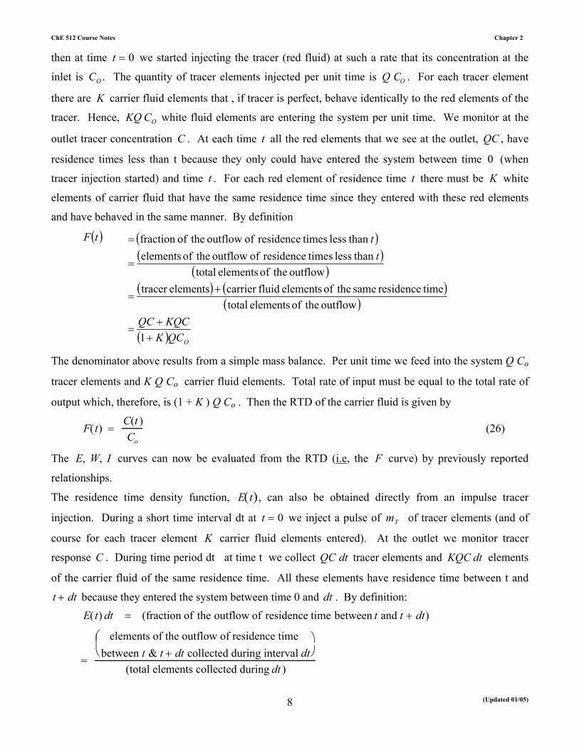
and have behaved in the same manner. By definition

( ) ( )( )

( )( ) ( )

( )

( ) OQCKKQCQC

tttF

++

=

+=

=

=

1

outflow theof elements total timeresidence same theof elements fluidcarrier elementstracer

outflow theof elements total than less timesresidence of outflow theof elements

than less timesresidence of outflow theoffraction

The denominator above results from a simple mass balance. Per unit time we feed into the system Q Co

tracer elements and K Q Co carrier fluid elements. Total rate of input must be equal to the total rate of

output which, therefore, is (1 + K ) Q Co . Then the RTD of the carrier fluid is given by

F( t) = C(t )Co

(26)

The E, W, I curves can now be evaluated from the RTD (i.e, the F curve) by previously reported

relationships.

The residence time density function, E t( ), can also be obtained directly from an impulse tracer

injection. During a short time interval dt at t = 0 we inject a pulse of mT of tracer elements (and of

course for each tracer element K carrier fluid elements entered). At the outlet we monitor tracer

response C . During time period dt at time t we collect QC dt tracer elements and KQC dt elements

of the carrier fluid of the same residence time. All these elements have residence time between t and

t + dt because they entered the system between time 0 and dt . By definition: E(t) dt = (fraction of the outflow of residence time between t and t + dt)

=

elements of the outflow of residence time between t & t + dt collected during interval dt

(total elements collected during dt )


(Updated 01/05)

9

=

(tracer elements in the outflow collected during time dt at t) +carrier fluid elements of the sameresidence time as tracer elements

(total elements collected during dt )

E(t) dt =QC dt + K QCdt

m T + K m T

=Q C dt (1+K)m T (1 + K)

E(t) =QCm T

(27)

Other functions F, I, W can now be derived from the E curve using previously reported relationships.

The total mass balance on tracer in a pulse injection requires that all the tracer injected must eventually

emerge, which is the same as requiring that 0

∞

∫ E (t) dt =1 . This formula is used to check the tracer

mass balance and ensure that the experiment is executed properly. The formula can also be used (when

one is confident that tracer is indeed conserved) to determine the unknown flow rate:

Q =m T

C (t)dt0

∞

∫ (28)

Whenever the mass balance for the tracer is not properly satisfied the tracer test does not represent a

proper way of determining the E curve. Various pitfalls were discussed by Curl, R. and McMillan, M.

L. (AIChE J., 12, 819, 1966).

The washout curve, W t( ) , can of course be obtained from the step-up tracer test by subtracting the F t( )

curve from unity, W = 1− F . This produces inaccurate results at large times because of subtraction of

numbers of the similar order of magnitude since t → ∞lim F =1 . Therefore, W t( ) can be obtained directly by a

step-down tracer test. Imagine that at the end of the step-up test both the inlet and exit tracer

concentration are CO . Now at t = 0 we start the stop watch and reduce the inlet tracer concentration to

0. Then all the tracer elements appearing at the outflow at time t are older than t since they have

entered the system before time 0. Due to linearity and perfect behavior of the tracer, for each tracer

element there are K carrier fluid elements of the same residence time. By definition:

)(tW =(fraction of the outflow that has residence times larger than t )= oo C

CCQKCQK

=++

)1()1(

(29)

The area under the washout curve gives the mean residence time:


(Updated 01/05)

10

t =VQ

= W (t ) dtO

∞

∫ (30)

Based on the previously derived relationships you should be able to prove the above.

The I t( ) curve can be evaluated readily using the step-down tracer test, its integral and eq (31):

I (t) =1t

W (t) (31)

The I t( ) curve is often determined directly in biomedical applications by injecting a pulse of tracer mTo

at time 0, and by monitoring the response of the whole system (not the outflow) which is proportional to

the mass of tracer remaining at time t , mT . Then:

I (t ) =m T (t)m T o

(32)

Some Other Items of Interest:

Perfect tracer -detectable, yet same behavior as carrier fluid and at infinite dilution.

Radioactive tracers - half life >> t (only exception positron emitters).

Electrolytes - conductivity meters (cast epoxy tubular body carbon ring electrodes and female pipe

threaded ends with a self balancing bridge working at 1000 Hz to eliminate polarization).

Dyes - colorimetric detectors and spectrophometer may give nonlinear response.

- thermal conductivity detectors.

- flame ionization detectors (organics)

- R ( CO2 , SO2 , NH3 in mixture of diatomic gases) two channel design preferred.

2.3 How To Derive Age Density Functions We know what the age density functions for the two ideal reactors (PFR and CSTR) look like. Using

these we can derive the age density functions for a generalized compartmental model with time lags. By

this we mean that if we have evidence or reason to believe that a real flow system or reactor can be

represented by a set of CSTR's (well mixed compartments) and PFR's (time lags) in series or parallel we

can readily derive an E curve for any such combination.

Here, and in later applications, it is very useful to use Laplace transforms defined by


(Updated 01/05)

11

E (s ) = L E (t ){ } = e − s t E (t ) d tO

∞

∫ (33)

Any network of CSTR's and PFR's consists of: elements in parallel, elements in series, split points and

mixing points (where points are considered to have no volume). The rules for dealing with these are

explained below.

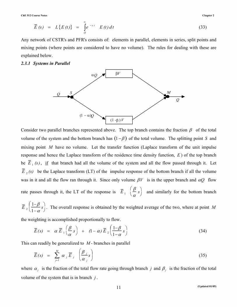
2.3.1 Systems in Parallel

V

Q

αQ

(1 − α)Q

Μ

Q

β(1 - ) V

β

S

Consider two parallel branches represented above. The top branch contains the fraction β of the total

volume of the system and the bottom branch has 1 −β( ) of the total volume. The splitting point S and

mixing point M have no volume. Let the transfer function (Laplace transform of the unit impulse

response and hence the Laplace transform of the residence time density function, E ) of the top branch

be E 1 (s ) , if that branch had all the volume of the system and all the flow passed through it. Let

E 2 (s) be the Laplace transform (LT) of the impulse response of the bottom branch if all the volume

was in it and all the flow ran through it. Since only volume βV is in the upper branch and Qα flow

rate passes through it, the LT of the response is E 1βα

s

and similarly for the bottom branch

E 21−β1−α

s

. The overall response is obtained by the weighted average of the two, where at point M

the weighting is accomplished proportionally to flow.

E (s) = α E 1βα

s

+ (1 − α ) E 2

1−β1−α

s

(34)

This can readily be generalized to M - branches in parallel

E (s) =j=1

M

∑ α j E j

β j

α j

s

(35)

where α j is the fraction of the total flow rate going through branch j and β j is the fraction of the total

volume of the system that is in branch j .


(Updated 01/05)

12

We build block diagrams for flow pattern representation out of two ideal patterns (plug flow and

complete backmixing) or their combinations. We know the E θ (θ ) curves for our building blocks with

θ = t / t where t is the total mean residence time. They are the impulse responses of a PFR and a

CSTR. If the building block is a subsystem then the mean residence time is t sub = βα

t (β = fraction of

total system's volume present in subsystem, α - multiple or fraction of total system's throughput that

flows through the subsystem) so that θ sub = t / t sub =α tβ t

=αβ

θ . Then the subsystem's dimensionless

impulse response is: Eθ (αβ

θ ) .

More generally speaking we are stating that if the dimensionless response of a system with volume V

and flow rate Q that exhibits a certain flow pattern is Eθ θ( ), then the impulse response of the same

system when it is a subsystem, i.e. a building block within a larger system) (containing fraction β of the

volume of the whole system and with flow rate of αQ going through it) is given by Eθαβ

θ

.

The dimensional impulse response of the subsystem then is given by

E θ θ sub( )d θ sub = E sub (t ) dt (36)

When α = β = 1 we get the whole system's response.

E (t) = 1t

E θ t / t ( ) (37)

Thus, by replacing t by β t / α we get Esub (t) from E(t) . Now the previously stated relation for the

Laplace transforms follows.

L E(t ){ }= e− st E(t ) dtO

∞

∫ = 1t

e− st Eθ (t / t )dt = E (s)O

∞

∫ (38)

L Esub (t){ }=αβt

e− s t Eθ αtβt

dt

O

∞

∫ =1t

e− β

αs

u

Eθut

du

O

∞

∫ = E sub βα

s

(39)

by replacing s with βα

s in E (s) we get E sub .

Also:

L Eθ θ( ){ } = e− sθ Eθ θ( )dθ = E θ s( )O

∞

∫ (40)


(Updated 01/05)

13

L Eθsub θ( ){ } = e− sθ Eθ

αβ

θ

dθ

O

∞

∫ =βα

e− β

αsu

Eθ du( )O

∞

∫ = βα

E θsub

βα

s

(41)

However the mean of Eθsub is not 1 but

βα

.

_______________________________________________________________________

Example

1. 2-CSTR's of different volume in two parallel branches:

V

Q

Q

Q

Μ

V

S

1

2

2

1

Q1 + Q2 = Q

α =Q 1

Q

V 1 + V 2 = V

β =V 1

V

Now E s( ) = α E 1βα

s

+ 1 − α( )E 2

1 − β1− α

s

where t 1 =βα

t , t 2 =1− β( )1 − α( )

t

E 1 s( ) = E 2 s( ) =1

1+ t i s; i =1 or 2

E s( )= α1

1+ βα

t s+ 1− α( ) 1

1 + 1− β1 − α

t s

E t( ) = L −1 E s( ){ }=α 2

β t e

−α tβ t +

1 − α( )1 − β( )t

2e

−1−α( )t1−β( )t

2.3.2 Systems in Series

Let us now consider a system in series consisting of two elements as shown below.


(Updated 01/05)

14

VQ V21

β= (1- ) VV2β= VV1 Let the transfer function of the first one be E 1 s( ) and of the second one E 2 s( ). If the first one

contains a fraction β of the total volume of the system then the system’s response in the Laplace

domain (transfer function) is given by

E s( )= E 1 β s( ) x E 2 (1 − β )s( ) (42)

In time domain this is:

E t( ) =O

t

∫1β

E 1τβ

1

1 − βE 2

t1 − β

−τ

1 − β

dτ (43)

This is the well known convolution theorem for linear systems.

The above rule can be readily generalized to N subsystems in series, each containing a fraction β j of

the total volume of the system. The overall transfer function is given by

E s( )= E j β j s( )j =1

S

∏ (44)

where E j s( ) is the Laplace transform of the impulse response of the j-th individual subsystem as if it

contained the whole volume of the system.

_____________________________________________________________________

Example:

Find the E-curve of N-equal sized CSTRs in series.

We know that for a single stirred tank of volume V and with flow rate Q the impulse response is

given by

E1 t( ) =1t

e− t / t

so that the transfer function is

E 1 s( ) =1

1+ t s

where t = V / Q.

For N equal size stirred tanks in series each tank contains β j =1N

fraction of the total volume. Hence

E j βs( ) = E jsN

=

1

1+t N

s


(Updated 01/05)

15

The overall transfer function is obtained by eq (44):

E s( )=1

1+t N

s

=1

1 + t N

s

Nj=1

N

∏

The overall impulse response then is obtained by inversion of the Laplace transform

E t( )= L−1 1

1 +t N

s

N

= Nt

NL−1 1

s +Nt

N

= Nt

N tN−1

N −1( )!e−Nt/t

The dimensionless E-curve is

Eθ θ( )= t E t θ( ) =N N

N −1( )!θ N−1e−Nθ

We can now use the above to derive the responses of N-CSTR's of equal size in series, CSTR's and

PFR's in parallel and systems with recycle.

In the example on nonideal stirred tank that follows the section on systems with recycle we will show

how to determine the parameters of the model from the experimentally determined E-curve and how to

use this in assessing reactor performance.


(Updated 01/05)

16

2.3.3 Systems with Recycle

Once you have mastered the derivation of the transfer function for subsystems in series and subsystems

in parallel, you should be able to handle systems with recycle. The only new “rule” is the splitting rule

where by if you split a stream each of the outgoing streams possesses the same transfer function.

Let us consider a general recycle system depicted below:

Q

2G

1GQ

V

S

RQ

(R+1)QM (R+1)QBV

( )Vβ−1 Flow rate Q flows through a recycle system (the system within the dashed box is the system with

recycle) of total volume V. Internally, at point M flow rate Q is joined by recycle flow rate, RQ, so that

the flow rate of (R+1)Q flows through the forward branch of the system that contains volume Vβ . At

splitting point S, R, Q, is recycled through the recycle branch of volume ( )Vβ−1 which flow rate Q

leaves the system. The transfer function of the forward branch is 1G (we mean by it

+ 11 RsG β ). The

transfer function of the recycle flow branch is 2G i.e. ( )

−

RsG β1

2 .

The transfer function of the total system is ( )sE .

Applying what we have learned so far, we note that for a normalized impulse injection of ( )tδ the

transfer function for the inlet is 1. The mass balance in the Laplace domain yields

( ) ( ) ERGEGR 11 12 +=+ (45)

This response ( )ER 1+ is obtained by the product (i.e. convolution in the time domain) of the transfer

function for the forward path, 1G , and the transfer function for the inlet stream after mixing point M.

The later is the sum of the transfer function for the fresh inlet stream (i.e. 1) and the product (i.e.

convolution in time domain) of the transfer function for the recycle branch, 2G , and the transfer

function for the exit stream, E , multiplied by R due to flow rate being RQ.

We can now solve eq (45) for the transfer function of the system E :

21

1

1 GGRRGE

−+= (46a)


(Updated 01/05)

17

Which can also be written as:

21

1

111

1

GGR

RG

RE

+−+

= (46b)

We recall that 21, GG are functions of ( )1+Rsβ and ( ) Rsβ−1 , respectively.

To get the impulse response in the time domain, inversion of equation (46a) or (46b) can be attempted

using the usual rules for Laplace transform inversion.

Often it is necessary to expand equation 46(b) by binomial theorem to get:

∑∞

=

++

=0

211 111

n

nnn

GGR

RGR

E (47)

Which can be rearranged to the following form:

∑∞

=

−⋅

+

=0

1211 1

1n

nnn

GGR

RR

E (48)

To obtain the impulse response in the time domain one can now invert the series in equation (48) term

by term.

Example

Consider a recycle system with volume Vβ in the forward branch and volume ( )Vβ−1 in the recycle

branch as sketch below. Plug flow occurs in both branches so that ( )

( ) Rst

Rst

eG

eGβ

β

−−

+−

=

=1

2

11

Plug Flow

Plug Flow

Vβ

( )Vβ−1 RQ

( ) QR 1+ Q

According to equation (48)

( ) ( )

∑∞

=

−−−+

−

+=

1

111

11

n

Rsnt

Rnstn

eeR

RR

Eββ

Inversion, term by term, yields

( ) ( ) ( )∑∞

=

−−−

+−

+=

1

1111

1n

n

Rnt

Rntt

RR

RtE ββδ


(Updated 01/05)

18

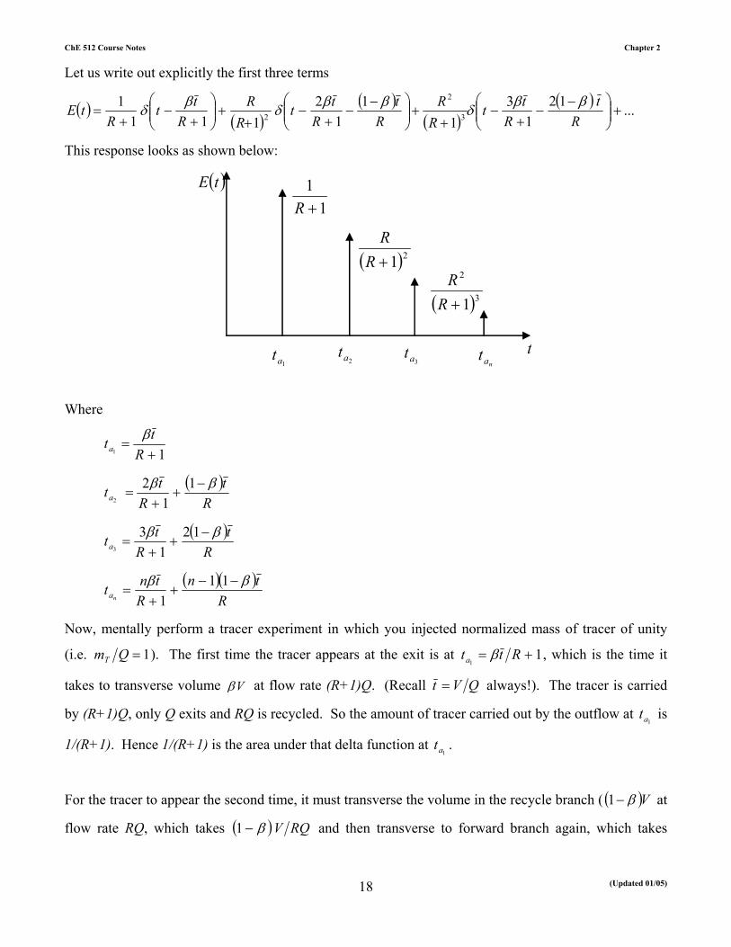
Let us write out explicitly the first three terms

( )( )

( )( )

( ) ...121

31

11

2111

13

2

2 +

−−

+−

++

−−

+−

++

+

−+

=R

tR

ttR

RR

tR

ttR

RR

ttR

tE ββδββδβδ

This response looks as shown below:

11+R

( )21+RR

( )3

2

1+RR

t

( )tE

1at 2at 3at

nat

Where

11 +

=R

ttaβ

( )R

tR

ttaββ −

++

=1

12

2

( )R

tR

ttaββ −

++

=12

13

3

( )( )R

tnR

tntna

ββ −−+

+=

111

Now, mentally perform a tracer experiment in which you injected normalized mass of tracer of unity

(i.e. 1=QmT ). The first time the tracer appears at the exit is at 11

+= Rtta β , which is the time it

takes to transverse volume Vβ at flow rate (R+1)Q. (Recall QVt = always!). The tracer is carried

by (R+1)Q, only Q exits and RQ is recycled. So the amount of tracer carried out by the outflow at 1at is

1/(R+1). Hence 1/(R+1) is the area under that delta function at 1at .

For the tracer to appear the second time, it must transverse the volume in the recycle branch ( ( )Vβ−1 at

flow rate RQ, which takes ( ) RQVβ−1 and then transverse to forward branch again, which takes


(Updated 01/05)

19

another 1at . So ( )

RVtt aa

β−+=

1212

. The amount of tracer that now arrives at the exit is ( )1+RR

(remember ( )11 +R left at the first passage time) and again only the fraction 1

1+R

is recycled. So the

area under the second delta function at 2at is ( )21+RR . The reast follows by analogy.

We note that if we had only the response curve we could tell how much volume the recycle system has

associated with the forward and recycle branch. The difference

( ) constR

tR

tttnn aa =

−+

+=−

−

ββ 111

Since 11 +

=R

ttaβ

We know that if

11 aaa ttt

nn=−

−

All the volume is in the forward stream i.e. 1=β , Otherwise

( )R

tttt aaa nn

β−=−−

−

111

(*)

By dividing the areas under the first peak 1

11 +

=R

A with the area under the second peak ( )22 1+

=R

RA

we get

R

RAA 1

2

1 += (**)

We can use eqs (*) and (**) to get estimates for β and R.


(Updated 01/05)

20

Example of a Nonideal Stirred Tank Reactor

A reactor of volume V = 25 m3 25,000 lit( ) with flow rate Q =1000 lit / min = 1 m3 / min which was

designed to operate as a CSTR and give very high conversion for a 2nd order irreversible reaction ( A →

product) is operating poorly at xA = 0.75 . A pulse of mi = 250g of tracer is injected instantaneously

into the reactor. At the outlet the following exit concentration is measured for the tracer. Initially rapid

fluctuations within the first five seconds of very high tracer concentration are observed. Afterwards the

following data is obtained:

t(min) 10 20 30 40 50 60 70 80

c(mg / lit) 6.21 3.52 2.15 1.10 0.70 0.40 0.23 0.13

a) How can we model the old reactor?

b) If we had a perfect CSTR what volume do we need for xA = 0.75 ?

c) What volume of a perfect CSTR do we need to get conversion that currently is produced by the

well mixed region?

The rapid initial rise of tracer concentration in the outflow seems to suggest bypassing. The slope of

ln C vs t is

slope = - ln 1.06 / 0.01( )

85= − 0.0549

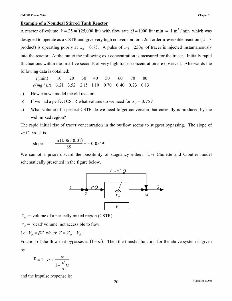
We cannot a priori discard the possibility of stagnancy either. Use Cholette and Cloutier model

schematically presented in the figure below.

Q

Μ

Q

S Vm

Vd

1 −α( ) Q

αQ

Vm = volume of a perfectly mixed region (CSTR)

Vd = 'dead' volume, not accessible to flow

Let Vm = βV where V = Vm + Vd .

Fraction of the flow that bypasses is 1 − α( ). Then the transfer function for the above system is given

by

E = 1 −α +α

1+ βα

t s

and the impulse response is:


(Updated 01/05)

21

E t( )= 1− α( ) δ t( )+α 2

βt e

−αtβt

where t =VQ

.

If we recognize that C t( )= miE t( )

Q, then:

C t( )= mi

Q 1 − α( ) δ t( )+

α 2

βt e

−α tβt

If we plot on semilog paper

ln C = ln mi

Qα( )2

βt

−

αβt

t , then − slope = 0.055 = αβ t

slope = S

Extrapolation of the exponential to t = 0 gives

I = Cexp 0( ) = miQ

α( )2

βt = 10.7 (mg / L) = 10.7x10−3 g / L( )

Cexp 0( )

S =

mi α( )Q

= IS

α = Qmi

IS

α = Qmi

Cexp 0( )

S =

1000250

10.7x10−3

0.055 = 0.778

α ≈ 0.78 1 − α = 0.22 of the flow bypasses the vessel

From the information given we have the mean residence time:

t =251

= 25 min

Hence, we can find now the fraction of the total volume, β , that is actively mixed.

αβt

= 0.055 β = α

0.055 t =

0.780.055 x 25

= 0.567 ≈ 0.57

β ≈ 0.57

Vactive = 0.57 x 25 = 14.25 m3

Vdead = 10.75 m3

Now we need to set the CSTR design equation in order to find the unknown rate parameters:


(Updated 01/05)

22

Vactive

Qactive

= βVα( )Q

= CAo xAr

kCAo2 1 − xAr( )2

Now xAr is the actual conversion produced by the reactor found in the stream leaving the active section

of the reactor before mixing with the bypass stream

kCAo = xAr

1 − xAr( )2 αβt

However, we must first relate this conversion xAr to the conversion produced by the reactor as a whole.

This requires a balance around the mixing point M. The stream αQ arriving from the reactor has

conversion xAr , the stream bypassing the reactor has conversion of zero. This balance can be

represented by:

1 − α( )FAo + α FAo 1 − xAr( ) = FAo 1 − xA( )

1 − α + α 1 − xAr( ) = 1 − xA

1 − α xAr = 1 − xA so that xAr = xA

α

We are told that xA = 0.75 . Then, for xA = 0.75 and α = 0.78

xAr = 0.750.78

= 0.96

kCAo = 0.96

1 − 0.96( )2 0.78

0.57 x 25 = 32.8 min −1( )

Recall that V = QxA

kCAo 1 − xA( )2 , Then

b) Vnew xA = 0.75( ) =

1,000 x 0.7532.8 1 − 0.75( )2 = 366 (lit) = 0.37 m3

c) Vnew xA = 0.96( ) = 1000 x 0.9632.8 1 − 0.96( )2 = 18,293 lit = 18.3 m3

________________________________________________________________________


(Updated 01/05)

23

2.3.4 Bypassing and Stagnancy

Let us consider now a single CSTR with bypassing. If the portion of the flow that bypasses is 1 − α( )

the schematic of the system is as follows:

QαQ

(1 − α)Q

Μ

Q

S V

and the impulse response and its transform are given below by eqs. (48) and (49). We expand the

transform (see eq (49)) to evaluate its moments, and we tabulate below the dimensionless variance of

the system as a function of the fraction of flow that bypasses which is 1 − α( ). Clearly, the

dimensionless variance is larger than one for a CSTR with bypassing indicating pathological behavior.

E t( ) = 1 − α( ) δ t( ) + α 2

t e−αt / t (49)

E s( ) = 1 − α + α

1 + t α

s = 1 − α + α 1 −

t α

s +t 2

α 2 s 2

= 1 − t s +

t 2

αs2 + O s3( ) (50)

By a simple technique that is illustrated later, we have evaluated the moments from the above Laplace

transform expansion as:

µ 0 = 1µ1 = t

µ 2 = 2t 2

α

σE2 =

2t 2

α − t 2 =

t 2 2 − α( )α

σ E2 =

σE2

t 2 =

2 − αα

1 − α 0 0.1 0.2 0.3 0.4 0.5 0.6 0.7 0.8 0.9σ E

2 1 1.22 1.5 1.86 2.33 3 4 5.67 9 19 Now let us consider a single CSTR with 'dead' volume. Such dead volume cannot be reached by tracer

or by reactant molecules.

QQ

V

Vm

d


(Updated 01/05)

24

Let Vd = βV , so β is the fraction of the total reactor volume that is for all practical purposes

inaccessible. Now the impulse response of the system is:

E t( )=1

1− β( )t e− t

1−β( )t (51)

and its Laplace transform is

E s( )=1

1 + 1− β( )t s = 1− 1 − β( )t s + 1 − β( )2t 2s2 + O s3( ) (52)

Recall that

( ) ( )∑∞

=

−=

0 !1

n

nn

n

sn

sE µ (53)

Hence, µ o =1 (54a)

µ1 = 1 −β( )t (54b)

µ 2 = 2 1− β( )2 t 2 (54c)

σ E2 =

µ2 − µ12

µ12 =1

(54d)

Now we detected the presence of dead volume not from the value of the variance but from the fact that

µ1 < t , i.e the central volume principle is violated. We may note, however, that the central volume

principle is never violated and, while a fraction β of the volume of the system may be difficult to

reach, i.e is relatively "stagnant", as long as that volume is a physical part of the flow system under

consideration it is never "dead", i.e it will be reached by at least a few elements of the fluid and,

hence, elements of the tracer if not by flow then at least by diffusion. The fascinating feature of the

central volume principle, which is little known, is that the zeroth moment of the tracer impulse

concentration at any point of a closed system is constant and equal to mT/Q where mT is the mass of

the instantaneous tracer injection and Q is the volumetric flow rate through the system. This means

that the area under the concentration response to an impulse injection is constant anywhere in the

system (i.e at all points of the system) and it implies that at points where the tracer concentration

response rises rapidly, high values will be of short duration, while where the response is barely

detectable, it lasts seemingly forever! This makes sense, as it says that if a point is readily accessible

and easy to get to, it is also easy to get out of and the converse is also true - if it is hard to get to a

point it is equally hard to get out. With this in mind let us say that our system has a stagnancy


(Updated 01/05)

25

Vd = βV which exchanges its contents very slowly with the main well mixed region Vm at a rate

αQ with α ≤ 1.

By setting up differential mass balances for the tracer in region Vm and Vd, normalizing tracer

concentrations in Vm and Vd by multiplying with Q/mT to get the impulse response, and by applying

the LaPlace transform and solving the equations in the LaPlace domain you should be able to show

that

E s( )=1+

βα

t s

1+ 1 +βα

t s +

β 1 − β( )α

t 2s2 (55)

By expanding the denominator via binomial series, multiplying the result with the numerator and

grouping items with equal power of s you should be able to get:

E s( )= 1− t s + 1+β 2

α

t 2 s2 + 0 s3( ) (56)

From the above series we readily identify the moments of the E-curve

10 =µ (57a)

t=1µ (57b)

22

2 12 t

+=

αβµ (57c)

Hence the dimensionless variance of the E-curve is

σ E2 =

µ 2 − µ12

µ12 =1 + 2

β 2

α> 1 (58)

Clearly no matter what volume fraction β is relatively stagnant, the dimensionless variance is always

greater than one. The quantity σ E2 − 1 is proportional to the square of the stagnant volume fraction

and inversely proportional to the ratio of the exchange flow rate α Q between the ideally mixed

region, Vm, and stagnant region, Vd, and the flow rate Q through the system, i.e inversely proportional

to α. However, while the dimensionless variance is larger than one, indicating pathological behavior,

the central volume principle is satisfied and µ1 = t . Hence, regarding stagnancy we can adopt a

simple empirical rule. We will get an indication of stagnancy (dead volume) either from the fact that

µ1 < t , in which case the variance can be anything, or if our data are accurate enough and µ1 = t , one

can detect stagnancy from σ E2 >1.


(Updated 01/05)

26

You should note that if α → ∞ , that is if the exchange flow rate α Q between Vm and Vd is infinitely

faster than flow rate through the system itself, Q, we recover σ E2 = 1 and as evident from the

expression for E s( ) we recover the perfect mixer response. After all infinitely fast (instantaneous)

mixing between all regions of the system is the definition of the perfect CSTR, so we should not be

surprised by this result.

It should be clear from the above discussion, however, that just from the fact that the dimensionless

variance is larger than one we cannot tell whether we deal with stagnancy or bypassing. To be able to

distinguish between the two we should examine the shape of the E-curve and especially of the

intensity fraction Λ .

It is tempting to talk about bypassing, if pathology is detected at small times, (e.g. a peak at small

times) and of stagnancy, if pathology is present at large times (e.g. a peak at very large times).

However, small and large time are ill defined. It may be tempting to say that if the problem is caused by

fluid residing less than the characteristic reaction time, τ R , in the vessel we have a bypassing problem,

and if the problem is caused by fluid of residence times order of magnitude larger than τr then

stagnancy is the culprit.

This argument can be summarized as follows:

k CAo

n −1 t >> 1 stagnancy model is justified

k CAon −1 t << 1 bypassing model is justified

One can argue that stagnancy is justified if there is a significant fraction of the outflow with the

residence times t much larger than characteristic reaction times i.e

E t( )dt > 0.1t = 1

kCon − 1

∞

∫ (59a)

1 − F1

kCon − 1

> 0.1 (59b)

Bypassing is then considered as a model if there is a significant fraction of fluid that emerges at times

much less than the characteristic reaction time


(Updated 01/05)

27

E t( ) dt > 0.1t=0t = 1

kCOn−1∫ (60a)

F tr( ) > 0.1 (60b)

However, if one adopts these definitions then even PFR can exhibit bypassing if t < tr , and CSTR can

exhibit both bypassing or stagnancy as illustrated below:

ECSTR t( ) = 1t

e−t / t

(61)

ECSTR t( )dt = − e t / t

tr

∞

∫ tr∞ = e −t r / t > 0.1

(62)

which certainly is true whenever

tr

t < ln 10 which would then indicate "stagnancy". Similarly, bypassing would be indicated

whenever

−e− t/t tr 0

= 1− e−tr /t > 0.1

0.9 > e − t r /t ; i.e. for all tr

t > ln

10.9

.

To preclude considering stagnancy and bypassing for a perfect mixer (CSTR), and to reserve stagnancy

and bypassing for pathological systems only, we say that only systems that are pathological

σ 2 > 1, ordΛdt

> 0

exhibit either stagnancy or bypassing depending on the criteria above.

Example

Let us consider again the ill fated mixed reactor of our Example problem that was represented by the

Cholette-Cloutier model.

Characteristic reaction time is:

τr = 1

kCAo

= 1

32.8 = 0.03 min = 1.8 s

Characteristic design process time

t = VQ

= 251

= 25 min


(Updated 01/05)

28

Actual characteristic process time

t p = Va

Qa

= 0.57 x 250.78 x 1

= 18.3 min

An actual ideal CSTR has in the outflow the following fraction of fluid of residence times between 0 and τR

ECSTR t( )dt0

τ R

∫ = 1t

e− t / t dt0

τ R

∫ = 1 − e−τ R / t

= 1 − e−0.03/25 = 1 − e−0.0012

= 1 − 0.9988 = 0.001

Our flow pattern in the above example problem yields an outflow with the fraction of residence times

between 0 and τ R of:

0

τ R

∫ E t( )d t =O

τ R

∫ 1 −α( )δ t( ) d t +0

τ R

∫α 2

β t e − α t / β t d t

= 1 − α + α 1 − e−ατ R /β t ( )

= 1 - 0.78 + 0.78 1 - e0.78 x 0.03/ 0.57 x 25( )

= 0.22 + 0.78 1 - e−0.001642( )

= 0.22 + 0.78 1 - 0.9984( ) = 0.22 + 0.001 = 0.221

Since this is much larger than 0.001 , and we know that the system is pathological, i.e σ 2 >1 , it is clear

that bypassing contributed significantly to our problem of low conversion.

Now let us examine the effect of stagnancy, which we suspect since µ1 < t

E t( )dt = 1 − α( )δ t( )dt + α 2

βt τ R

∞

∫τ R

∞

∫τ R

∞

∫ e−αt /βt dt

= 0 + αe−

ατ R

βt = 0.78e−0.001642 = 0.779

Indeed stagnancy also contributes to the problem.

Ultimately, the best way to check for pathological behavior (e.g. bypassing or stagnancy) is by

examination of the intensity function, Λ t( )

Lack of undesirable behavior is indicated by

d2 Λdt2 ≥ 0 (63)


(Updated 01/05)

29

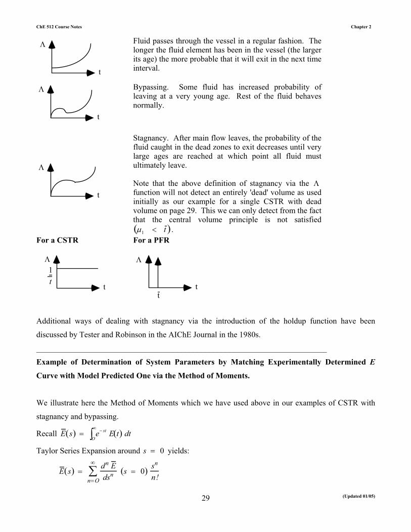
Λ

t

Fluid passes through the vessel in a regular fashion. The longer the fluid element has been in the vessel (the larger its age) the more probable that it will exit in the next time interval.

Λ

t

Bypassing. Some fluid has increased probability of leaving at a very young age. Rest of the fluid behaves normally.

Λ

t

Stagnancy. After main flow leaves, the probability of the fluid caught in the dead zones to exit decreases until very large ages are reached at which point all fluid must ultimately leave. Note that the above definition of stagnancy via the Λ function will not detect an entirely 'dead' volume as used initially as our example for a single CSTR with dead volume on page 29. This we can only detect from the fact that the central volume principle is not satisfied µ1 < t ( ) .

For a CSTR

Λ

t

1t

For a PFR Λ

tt-

Additional ways of dealing with stagnancy via the introduction of the holdup function have been

discussed by Tester and Robinson in the AIChE Journal in the 1980s.

________________________________________________________________________

Example of Determination of System Parameters by Matching Experimentally Determined E

Curve with Model Predicted One via the Method of Moments.

We illustrate here the Method of Moments which we have used above in our examples of CSTR with

stagnancy and bypassing.

Recall E s( ) = e− st E t( ) dtO

∞

∫

Taylor Series Expansion around s = 0 yields:

E s( ) = dn E dsn s = 0( ) sn

n!n=O

∞

∑


(Updated 01/05)

30

d oE ds o s = o = E s = o( ) = E t( )

O

∞

∫ dt = µ o

dE ds

s = o = − te− st E t( ) dtO

∞

∫

s = o

= t E t( )O

∞

∫ dt = - µ1

Hence,

µ n = −1( )n

dn E dsn

s= o

E s( ) = −1( )n µ n

n!sn = µ0 − µ1 s +

µ2

2s 2 −

µ 3

6s3

n= O

∞

∑ (A)

E s( )=n=O

∞

∑ d n E d s n 0( ) s n

n! (B)

By comparison of (A) and (B) moments can be obtained. For our stirred tank with bypassing and

stagnancy example,

E = 1−α +α

1 + βα

t s

E = 1 − α + α 1−β t α

s +β 2

α 2 t 2 s 2

E = 1−α +α − β t s +β 2

αt 2 s 2

E = 1 − β t s +β 2

αt 2 s 2

µ 0 = 1 µ 1 = β t

µ 2 =2β 2 t 2

α

σ 2 =2β 2 t 2

α− β 2 t 2 =

β 2 t 2

α2 − α[ ]

σ D2 =

σ 2

µ 12 =

β 2 t 2 2 − α[ ]α β 2 t 2 =

2 − αα

=2 − 0.78

0.78= 1.56

From the tracer experiment we get experimentally t exp = β t

σ t exp

2

t exp2 =

2 − αα

= 1.56

che 512 course notes chapter 2 2. characterization of macromixing 2.1 residence … · ·...

Documents