chem 302 - math 252 chapter 3 interpolation / extrapolation
TRANSCRIPT
Chem 302 - Math 252
Chapter 3Interpolation / Extrapolation
Interpolation / Extrapolation
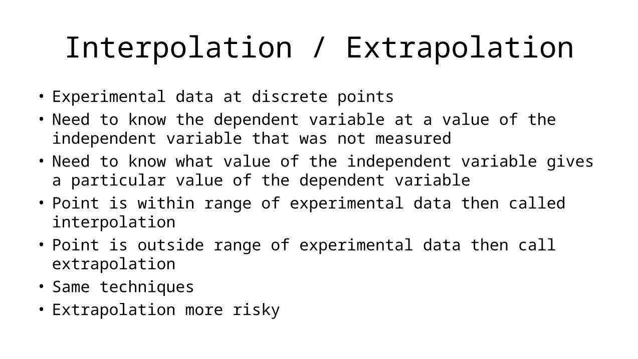
• Experimental data at discrete points• Need to know the dependent variable at a value of the independent
variable that was not measured• Need to know what value of the independent variable gives a particular
value of the dependent variable• Point is within range of experimental data then called interpolation• Point is outside range of experimental data then call extrapolation• Same techniques• Extrapolation more risky
Linear Interpolation
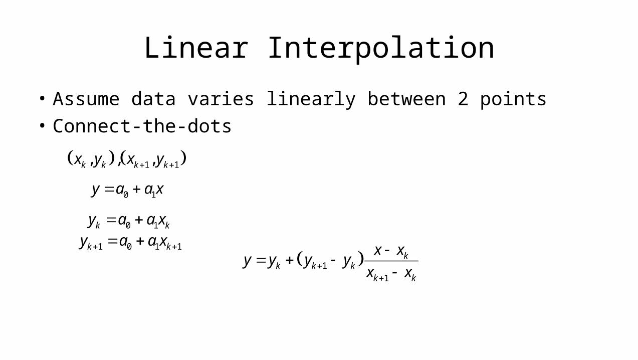
• Assume data varies linearly between 2 points
• Connect-the-dots 1 1, , ,k k k kx y x y
0 1y a a x
0 1k ky a a x
1 0 1 1k ky a a x 1
1
kk k k
k k
x xy y y y
x x
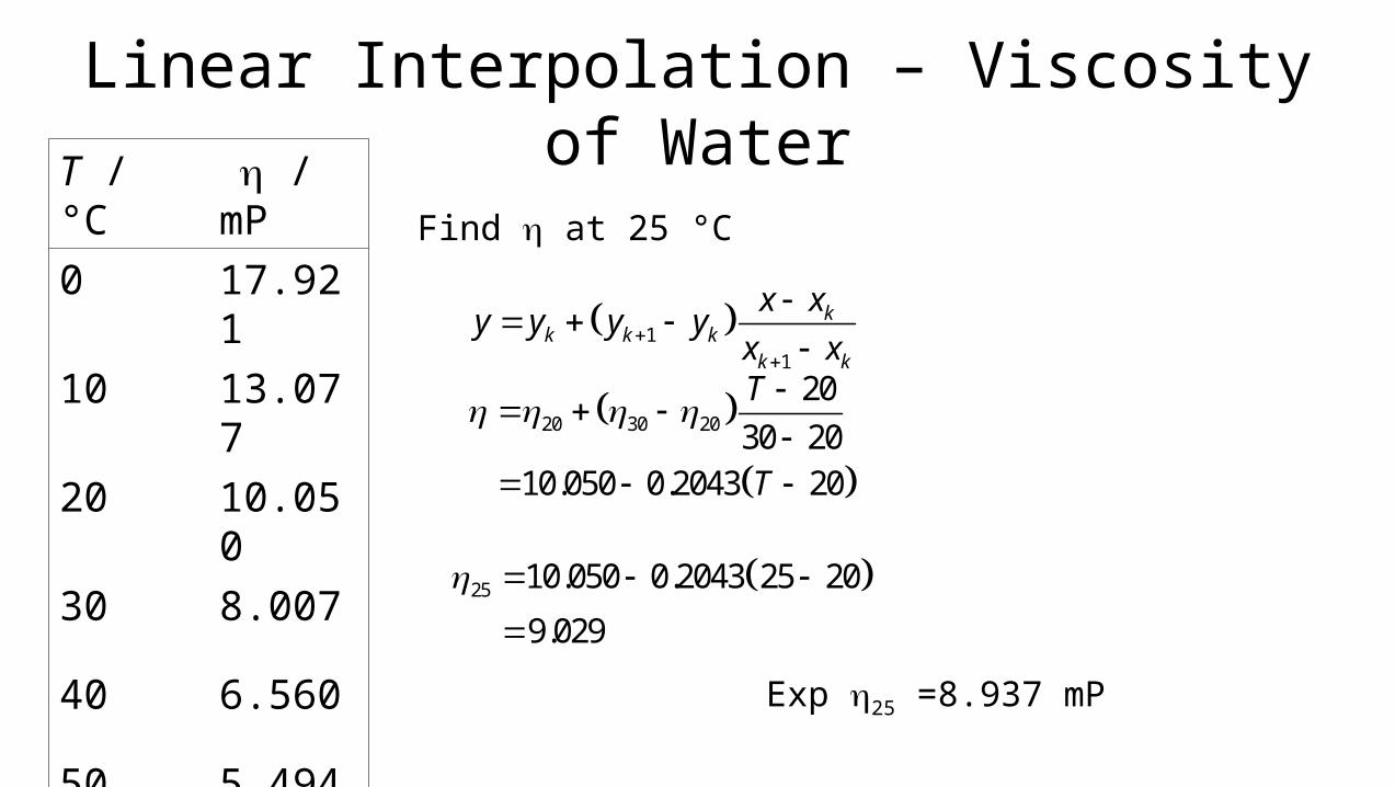
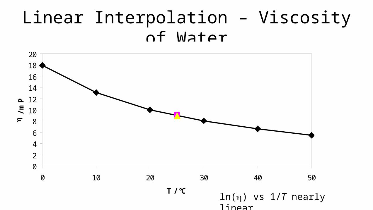
Linear Interpolation – Viscosity of WaterT / °C / mP
0 17.921
10 13.077
20 10.050
30 8.007
40 6.560
50 5.494
Find at 25 °C
11
kk k k
k k
x xy y y y
x x
20 30 20
20
30 2010.050 0.2043 20
T
T
25 10.050 0.2043 25 20
9.029
Exp 25 =8.937 mP
Linear Interpolation – Viscosity of Water
0
2
4
6
8
10
12
14
16
18
20
0 10 20 30 40 50
T / °C
/
mP
ln() vs 1/T nearly linear
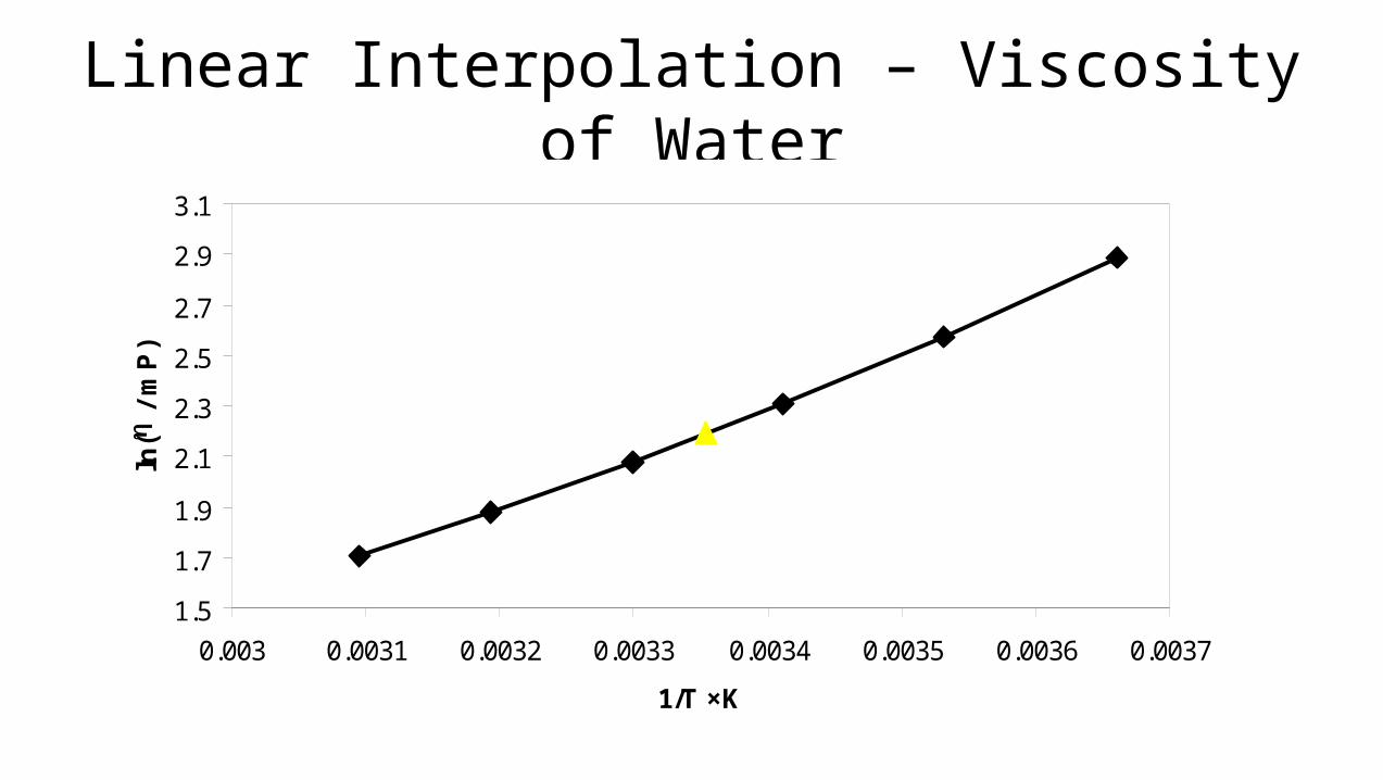
Linear Interpolation – Viscosity of Water
1.5
1.7
1.9
2.1
2.3
2.5
2.7
2.9
3.1
0.003 0.0031 0.0032 0.0033 0.0034 0.0035 0.0036 0.0037
1/T ×K
ln(
/ m
P)
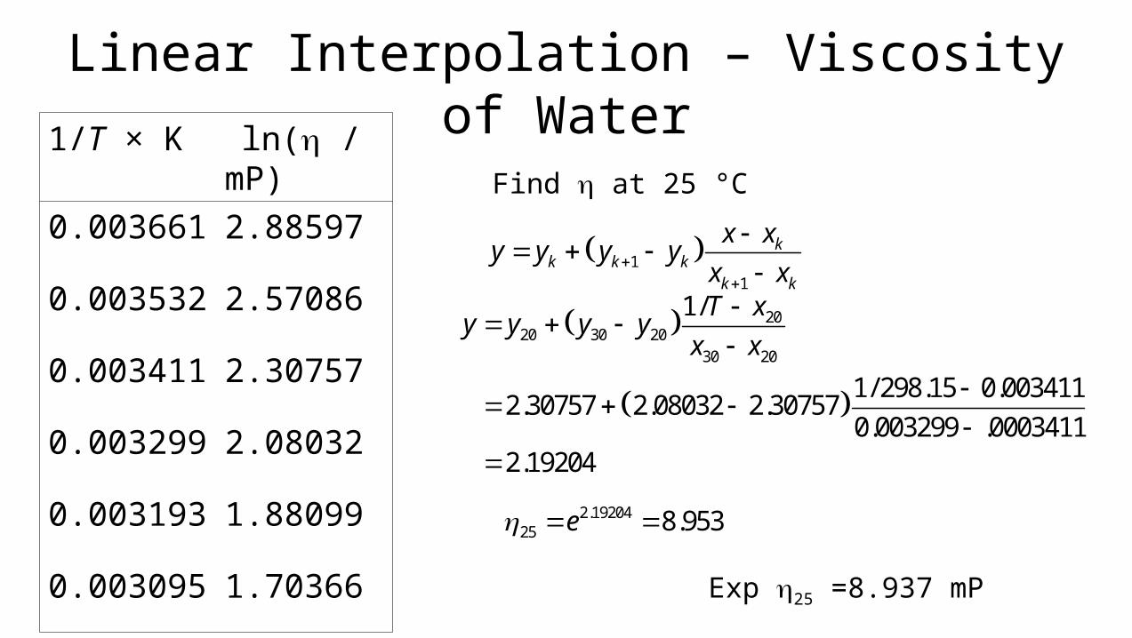
Linear Interpolation – Viscosity of Water1/T × K ln( / mP)
0.003661 2.88597
0.003532 2.57086
0.003411 2.30757
0.003299 2.08032
0.003193 1.88099
0.003095 1.70366
Find at 25 °C
11
kk k k
k k
x xy y y y
x x
2020 30 20
30 20
1/
1/ 298.15 0.0034112.30757 2.08032 2.30757
0.003299 .00034112.19204
T xy y y y
x x
2.1920425 8.953e
Exp 25 =8.937 mP
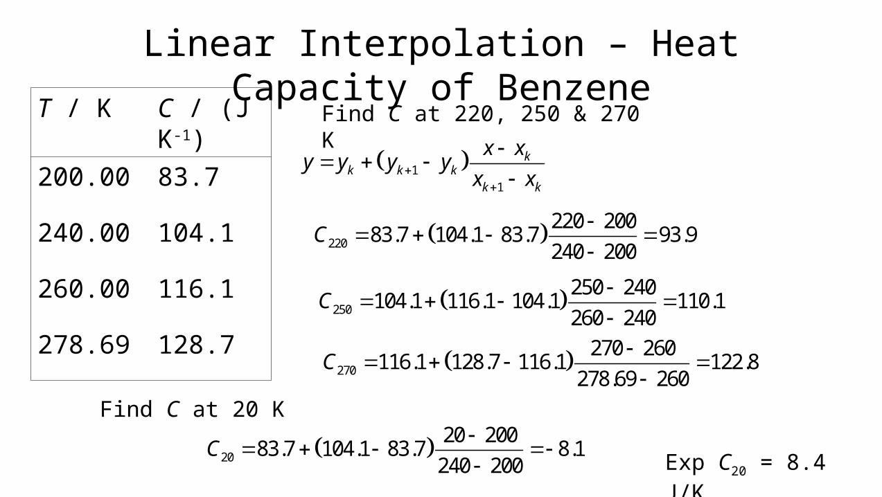
Linear Interpolation – Heat Capacity of BenzeneT / K C / (J K-1)
200.00 83.7
240.00 104.1
260.00 116.1
278.69 128.7
Find C at 220, 250 & 270 K
11
kk k k
k k
x xy y y y
x x
220
220 20083.7 104.1 83.7 93.9
240 200C
250
250 240104.1 116.1 104.1 110.1
260 240C
270
270 260116.1 128.7 116.1 122.8
278.69 260C
Find C at 20 K
20
20 20083.7 104.1 83.7 8.1
240 200C
Exp C20 = 8.4 J/K
Quadratic Interpolation
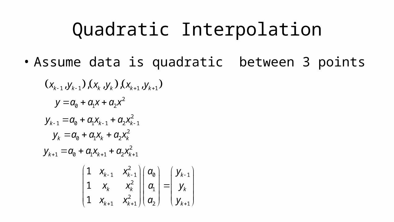
• Assume data is quadratic between 3 points
1 1 1 1, , , , ,k k k k k kx y x y x y
20 1 2y a a x a x
21 0 1 1 2 1k k ky a a x a x
20 1 2k k ky a a x a x
21 0 1 1 2 1k k ky a a x a x
21 1 0 1
21
21 1 2 1
1
1
1
k k k
k k k
k k k
x x a y
x x a y
x x a y
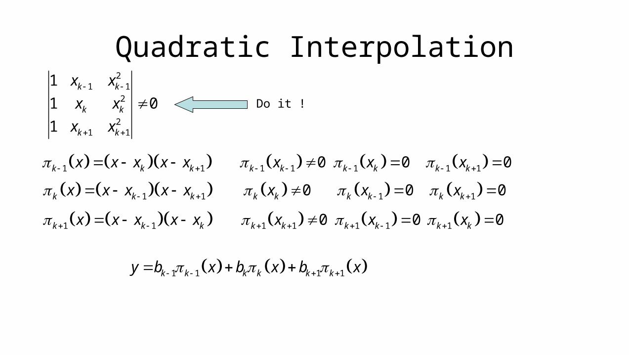
Quadratic Interpolation
1 1k k kx x x x x
21 1
2
21 1
1
1 0
1
k k
k k
k k
x x
x x
x x
Do it !
1 1k k kx x x x x
1 1k k kx x x x x
1 1 1 1 10 0 0k k k k k kx x x
1 10 0 0k k k k k kx x x
1 1 1 1 10 0 0k k k k k kx x x
1 1 1 1k k k k k ky b x b x b x
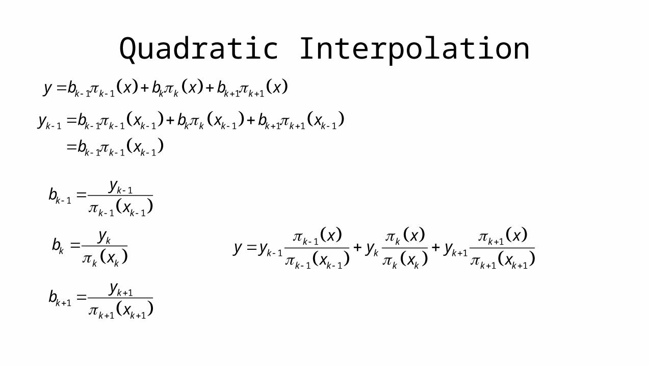
Quadratic Interpolation 1 1 1 1k k k k k ky b x b x b x
1 1 1 1 1 1 1 1
1 1 1
k k k k k k k k k k
k k k
y b x b x b x
b x
1
11 1
kk
k k
yb
x
k
kk k
yb
x
1
11 1
kk
k k
yb
x
1 11 1
1 1 1 1
k k kk k k
k k k k k k
x x xy y y y
x x x
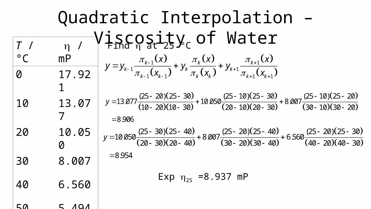
Quadratic Interpolation – Viscosity of WaterT / °C / mP
0 17.921
10 13.077
20 10.050
30 8.007
40 6.560
50 5.494
Find at 25 °C
Exp 25 =8.937 mP
1 11 1
1 1 1 1
k k kk k k
k k k k k k
x x xy y y y
x x x
(25 20) 25 30 (25 10) 25 30 (25 10) 25 2013.077 10.050 8.007
10 20 10 30 20 10 20 30 30 10 30 20
8.906
y
(25 30) 25 40 (25 20) 25 40 (25 20) 25 3010.050 8.007 6.560
20 30 20 40 30 20 30 40 40 20 40 30
8.954
y
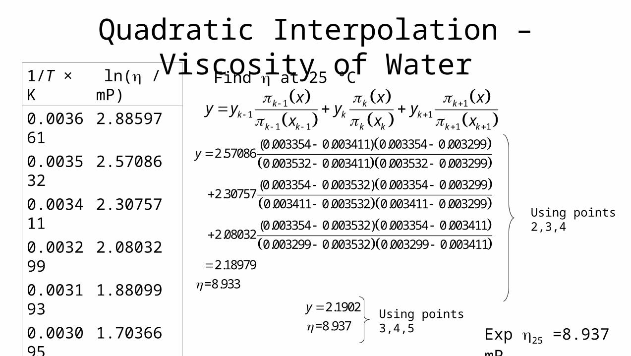
Quadratic Interpolation – Viscosity of Water1/T × K ln( / mP)
0.003661 2.88597
0.003532 2.57086
0.003411 2.30757
0.003299 2.08032
0.003193 1.88099
0.003095 1.70366
Find at 25 °C
Exp 25 =8.937 mP
1 11 1
1 1 1 1
k k kk k k
k k k k k k
x x xy y y y
x x x
(0.003354 0.003411) 0.003354 0.0032992.57086
0.003532 0.003411 0.003532 0.003299
(0.003354 0.003532) 0.003354 0.0032992.30757
0.003411 0.003532 0.003411 0.003299
(0.003354 0.003532) 0.003354 0.003412.08032
y
1
0.003299 0.003532 0.003299 0.003411
2.18979
=8.933
2.1902
=8.937
y
Using points 2,3,4
Using points 3,4,5
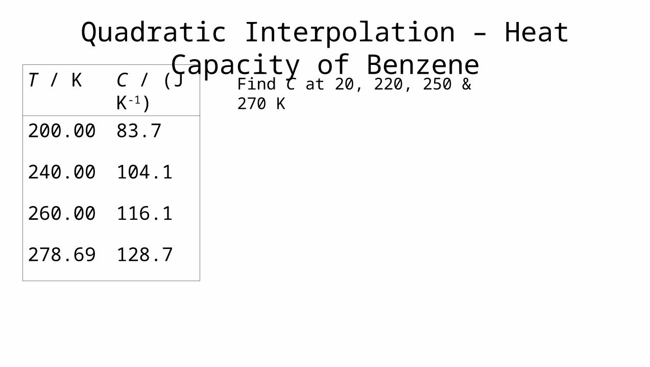
Quadratic Interpolation – Heat Capacity of BenzeneT / K C / (J K-1)
200.00 83.7
240.00 104.1
260.00 116.1
278.69 128.7
Find C at 20, 220, 250 & 270 K
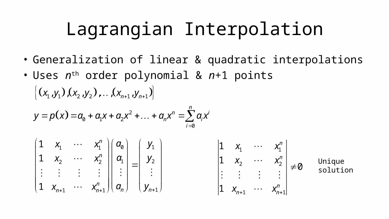
Lagrangian Interpolation
• Generalization of linear & quadratic interpolations• Uses nth order polynomial & n+1 points
1 1 2 2 1 1, , , , , ,n nx y x y x y
20 1 2
0
nn i
n ii
y p x a a x a x a x a x
0 11 1
1 22 2
11 1
1
1
1
n
n
nn nn n
a yx x
a yx x
a yx x
1 1
2 2
1 1
1
10
1
n
n
nn n
x x
x x
x x
Unique solution
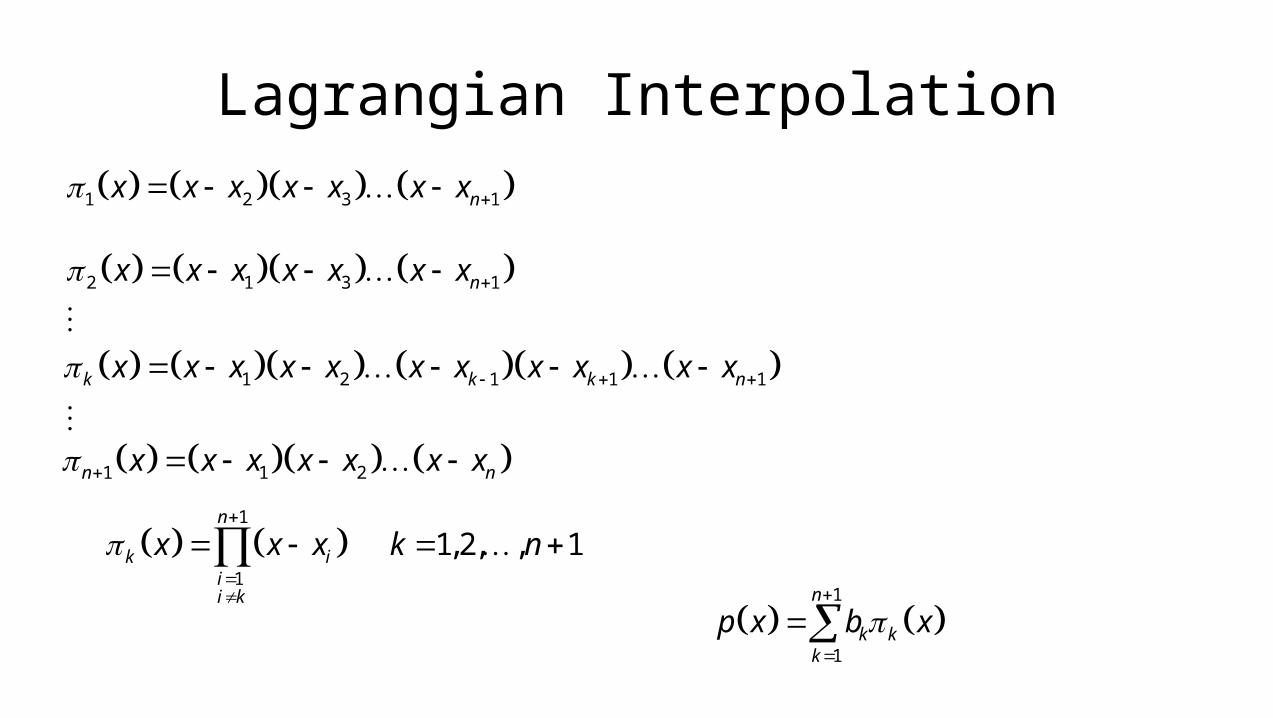
Lagrangian Interpolation
1 2 3 1nx x x x x x x
1
1
n
k kk
p x b x
2 1 3 1nx x x x x x x
1 2 1 1 1k k k nx x x x x x x x x x x
1 1 2n nx x x x x x x
1
1
1,2, , 1n
k iii k
x x x k n
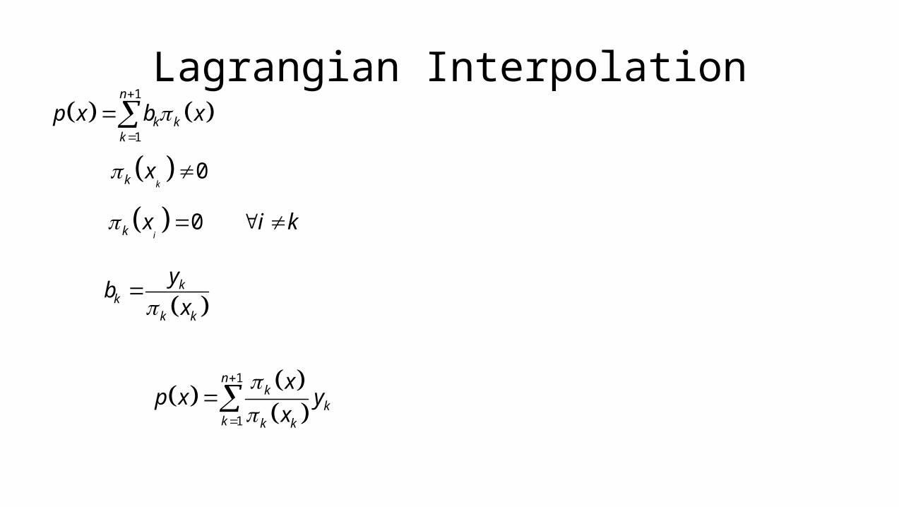
Lagrangian Interpolation
k
kk k
yb
x
1
1
n
k kk
p x b x
0kk x
0ik x i k
1
1
nk
kk k k
xp x y
x
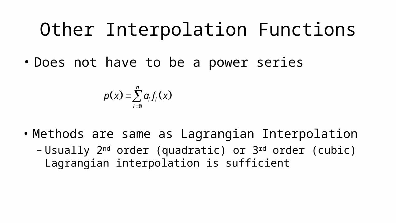
Other Interpolation Functions
• Does not have to be a power series
0
n
i ii
p x a f x
• Methods are same as Lagrangian Interpolation– Usually 2nd order (quadratic) or 3rd order (cubic) Lagrangian
interpolation is sufficient
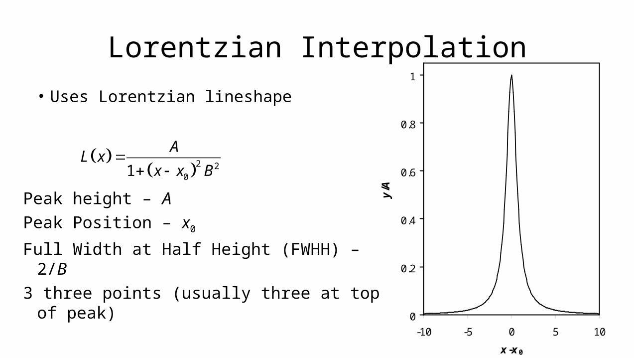
Lorentzian Interpolation
• Uses Lorentzian lineshape
2 2
01
AL x
x x B
0
0.2
0.4
0.6
0.8
1
-10 -5 0 5 10
x -x 0
y/ A
Peak height – A
Peak Position – x0
Full Width at Half Height (FWHH) – 2/B
3 three points (usually three at top of peak)
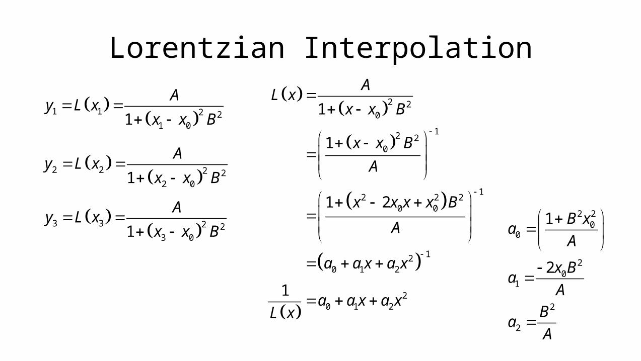
Lorentzian Interpolation
1 1 2 2
1 01
Ay L x
x x B
2 2 2 2
2 01
Ay L x
x x B
3 3 2 2
3 01
Ay L x
x x B
2 20
12 20
12 2 2
0 0
120 1 2
20 1 2
1
1
1 2
1
AL x
x x B
x x B
A
x x x x B
A
a a x a x
a a x a xL x
2 20
0
20
1
2
2
1
2
B xa
A
x Ba
A
Ba
A
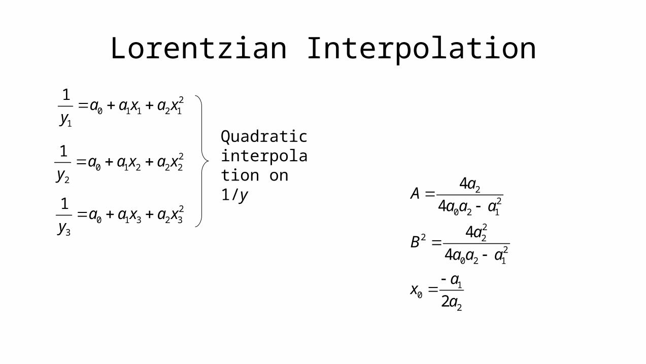
Lorentzian Interpolation
20 1 1 2 1
1
1a a x a x
y
22
0 2 1
22 2
20 2 1
10
2
4
4
4
4
2
aA
a a a
aB
a a a
ax
a
20 1 2 2 2
2
1a a x a x
y
20 1 3 2 3
3
1a a x a x
y
Quadratic interpolation on 1/y
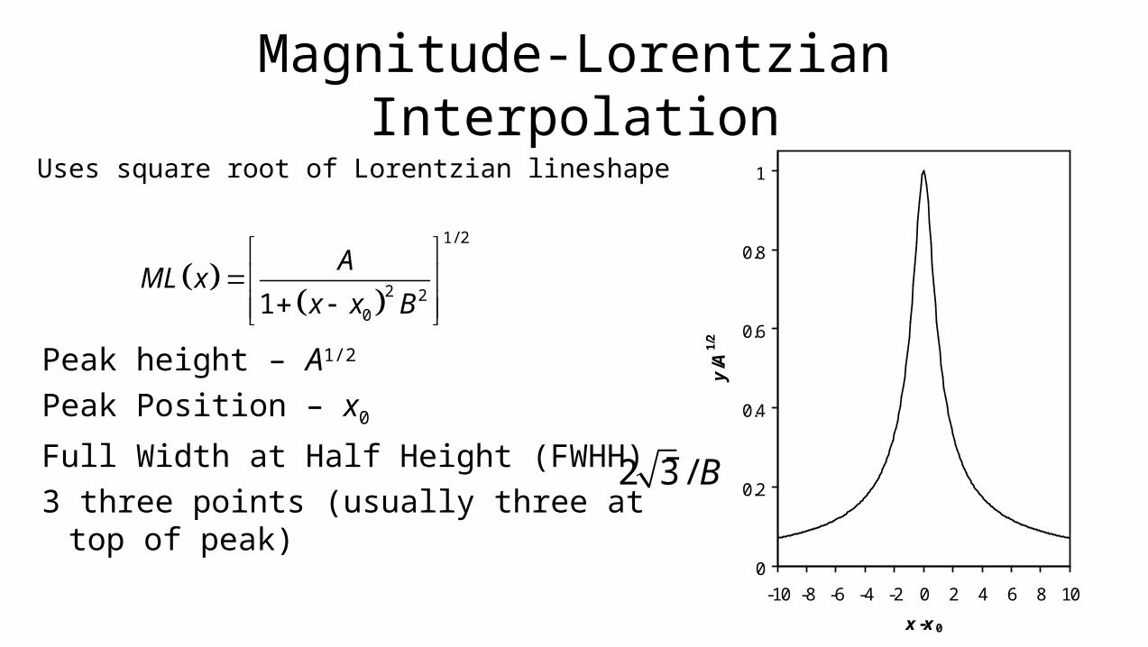
Magnitude-Lorentzian Interpolation
Uses square root of Lorentzian lineshape
1/ 2
2 201
AML x
x x B
Peak height – A1/2
Peak Position – x0
Full Width at Half Height (FWHH) –
3 three points (usually three at top of peak)0
0.2
0.4
0.6
0.8
1
-10 -8 -6 -4 -2 0 2 4 6 8 10
x -x 0
y/ A
1/2
2 3 / B
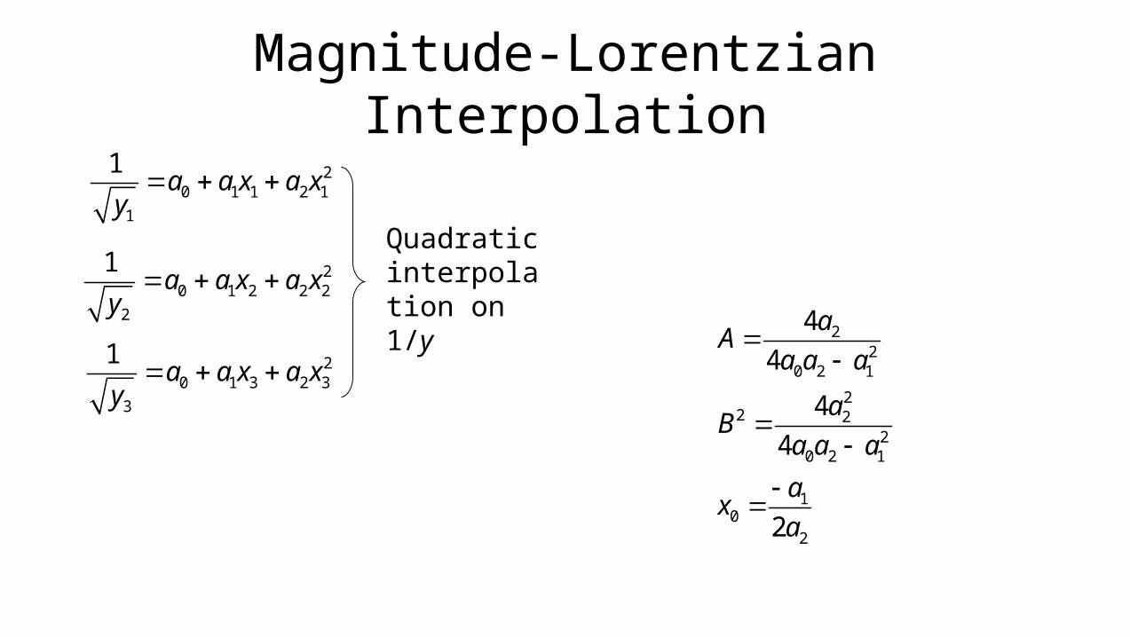
Magnitude-Lorentzian Interpolation
20 1 1 2 1
1
1a a x a x
y
22
0 2 1
22 2
20 2 1
10
2
4
4
4
4
2
aA
a a a
aB
a a a
ax
a
20 1 2 2 2
2
1a a x a x
y
20 1 3 2 3
3
1a a x a x
y
Quadratic interpolation on 1/y
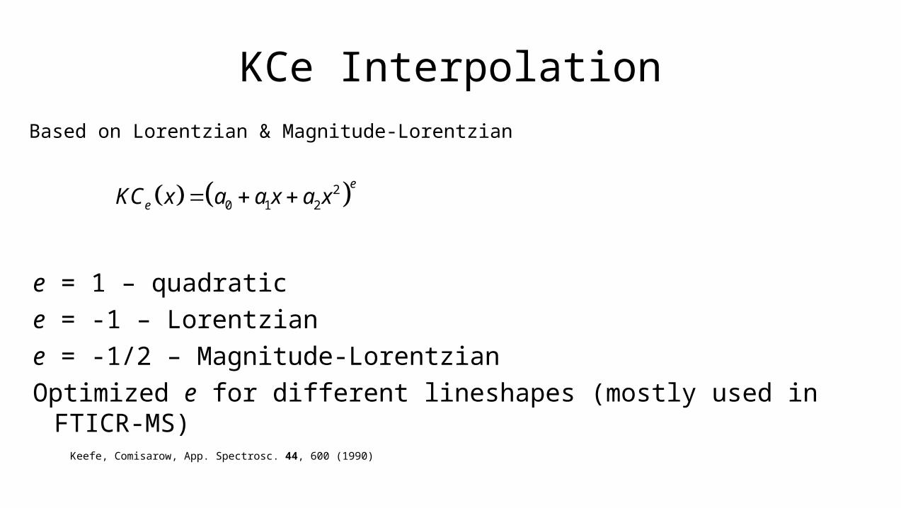
KCe Interpolation
Based on Lorentzian & Magnitude-Lorentzian
20 1 2
e
eKC x a a x a x
e = 1 – quadratic
e = -1 – Lorentzian
e = -1/2 – Magnitude-Lorentzian
Optimized e for different lineshapes (mostly used in FTICR-MS)Keefe, Comisarow, App. Spectrosc. 44, 600 (1990)
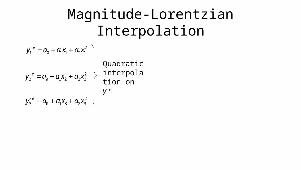
Magnitude-Lorentzian Interpolation
21 0 1 1 2 1ey a a x a x
22 0 1 2 2 2ey a a x a x
23 0 1 3 2 3ey a a x a x
Quadratic interpolation on y-e
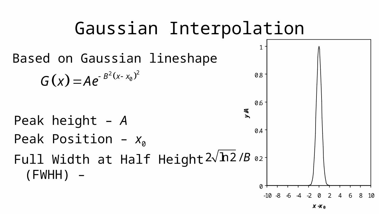
Gaussian Interpolation
Based on Gaussian lineshape
220B x xG x Ae
Peak height – A
Peak Position – x0
Full Width at Half Height (FWHH) – 2 ln 2 / B
0
0.2
0.4
0.6
0.8
1
-10 -8 -6 -4 -2 0 2 4 6 8 10
x -x 0
y/ A
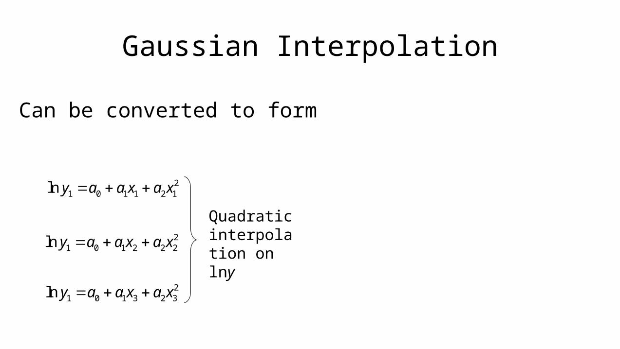
Gaussian Interpolation
21 0 1 1 2 1ln y a a x a x
21 0 1 2 2 2ln y a a x a x
21 0 1 3 2 3ln y a a x a x
Quadratic interpolation on lny
Can be converted to form
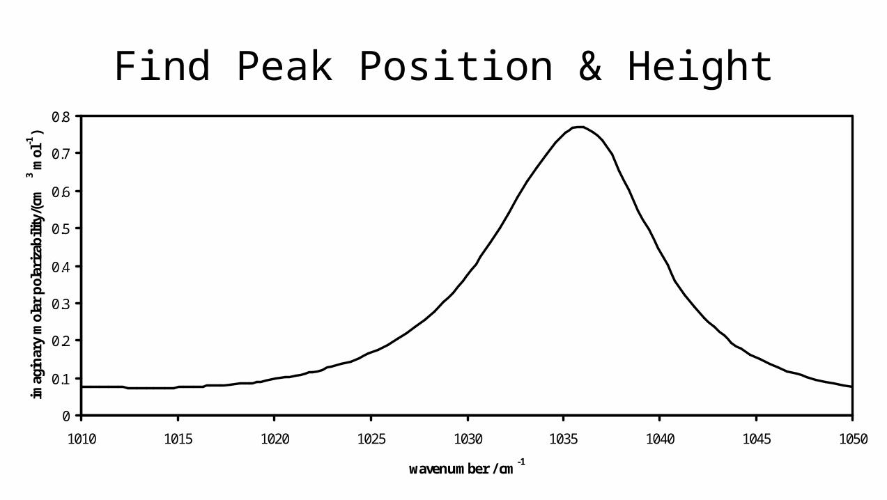
Find Peak Position & Height
0
0.1
0.2
0.3
0.4
0.5
0.6
0.7
0.8
1010 1015 1020 1025 1030 1035 1040 1045 1050
wavenumber / cm-1
imag
inar
y m
olar
pol
ariz
abili
ty/(
cm3 m
ol-1
)
0.69
0.7
0.71
0.72
0.73
0.74
0.75
0.76
0.77
0.78
1034.5 1035.5 1036.5 1037.5
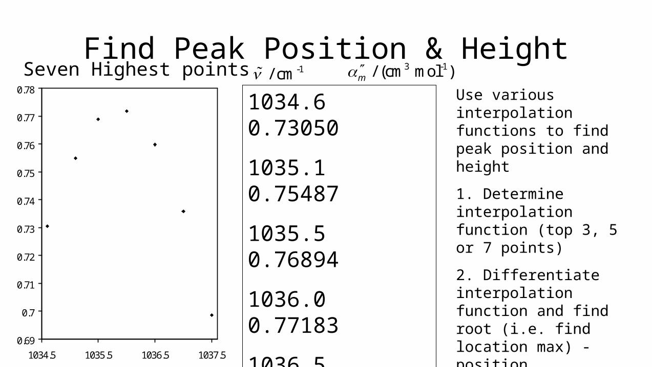
Find Peak Position & HeightSeven Highest points -1 / cm 3 -1 / (cm mol )m
1034.6 0.73050
1035.1 0.75487
1035.5 0.76894
1036.0 0.77183
1036.5 0.75979
1037.0 0.73585
1037.5 0.69860
Use various interpolation functions to find peak position and height
1. Determine interpolation function (top 3, 5 or 7 points)
2. Differentiate interpolation function and find root (i.e. find location max) - position
3.Evaluate interpolation function at peak position (height)
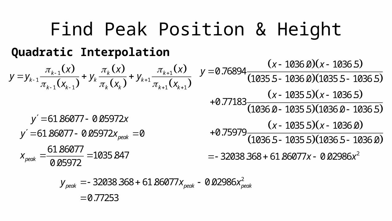
Find Peak Position & HeightQuadratic Interpolation
1 11 1
1 1 1 1
k k kk k k
k k k k k k
x x xy y y y
x x x
2
1036.0 1036.50.76894
1035.5 1036.0 1035.5 1036.5
1035.5 1036.50.77183
1036.0 1035.5 1036.0 1036.5
1035.5 1036.00.75979
1036.5 1035.5 1036.5 1036.0
32038.368 61.86077 0.02986
x xy
x x
x x
x x
61.86077 0.05972y x 61.86077 0.05972 0
61.860771035.847
0.05972
peak
peak
y x
x
232038.368 61.86077 0.02986
0.77253
peak peak peaky x x
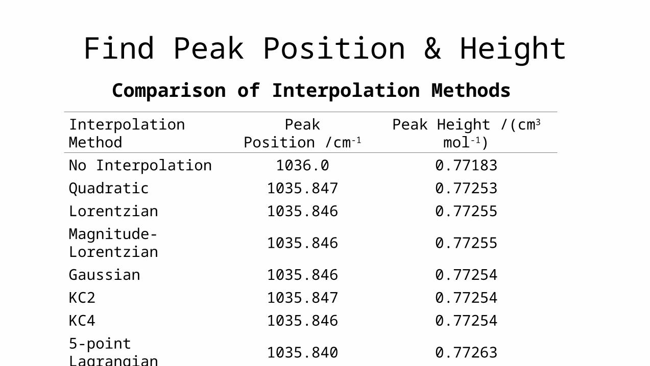
Find Peak Position & HeightComparison of Interpolation Methods
Interpolation Method Peak Position /cm-1 Peak Height /(cm3 mol-1)
No Interpolation 1036.0 0.77183
Quadratic 1035.847 0.77253
Lorentzian 1035.846 0.77255
Magnitude-Lorentzian 1035.846 0.77255
Gaussian 1035.846 0.77254
KC2 1035.847 0.77254
KC4 1035.846 0.77254
5-point Lagrangian 1035.840 0.77263
7-point Lagrangian 1035.834 0.77270
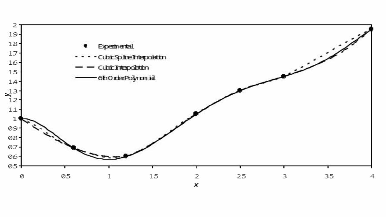
• So far methods have used a moving window of subset of data– May be discontinuous at edges of windows– Causes jagged plots
• Spline interpolation forces slopes (and in some cases higher derivatives) to match at edges of windows– Creates smooth plots
Spline Interpolation
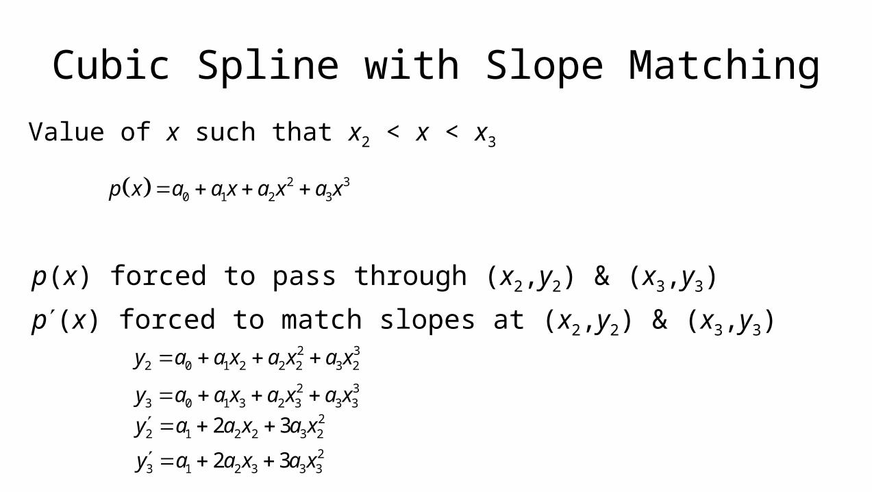
Cubic Spline with Slope Matching
Value of x such that x2 < x < x3
2 30 1 2 3p x a a x a x a x
p(x) forced to pass through (x2,y2) & (x3,y3)
p(x) forced to match slopes at (x2,y2) & (x3,y3)2 3
2 0 1 2 2 2 3 2y a a x a x a x 2 3
3 0 1 3 2 3 3 3y a a x a x a x 2
2 1 2 2 3 22 3y a a x a x 2
3 1 2 3 3 32 3y a a x a x
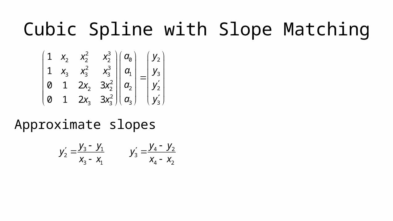
Cubic Spline with Slope Matching
Approximate slopes
3 12
3 1
y yy
x x
2 30 22 2 2
2 31 33 3 3
22 22 2
23 33 3
1
1
0 1 2 3
0 1 2 3
a yx x x
a yx x x
a yx x
a yx x
4 23
4 2
y yy
x x
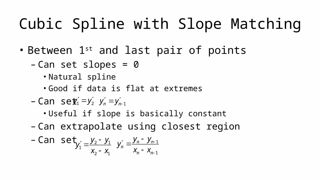
Cubic Spline with Slope Matching
• Between 1st and last pair of points– Can set slopes = 0
• Natural spline
• Good if data is flat at extremes
– Can set • Useful if slope is basically constant
– Can extrapolate using closest region– Can set
1 2y y 1n ny y
2 11
2 1
y yy
x x
1
1
n nn
n n
y yy
x x
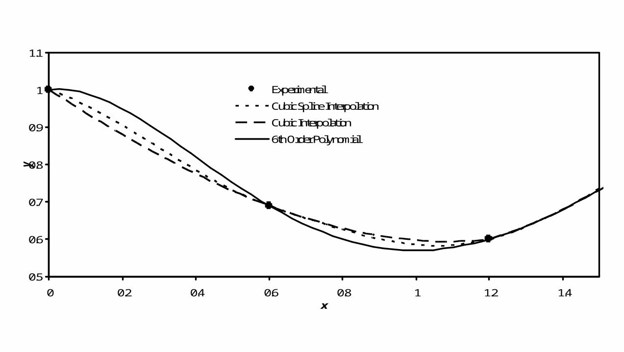
0.5
0.6
0.7
0.8
0.9
1
1.1
0 0.2 0.4 0.6 0.8 1 1.2 1.4x
y
Experimental
Cubic Spline Interpolation
Cubic Interpolation
6th Order Polynomial
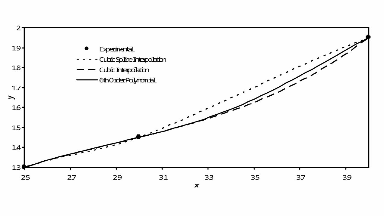
1.3
1.4
1.5
1.6
1.7
1.8
1.9
2
2.5 2.7 2.9 3.1 3.3 3.5 3.7 3.9x
y
Experimental
Cubic Spline Interpolation
Cubic Interpolation
6th Order Polynomial