chemical, biological, and materials engineering thermodynamics
DESCRIPTION
This book is an outgrowth of the authors’ sense that the topics covered by the majority of traditional engineering thermodynamics texts have evolved only slightly over the last several decades. The age of “molecular manufacturing” is here, and it is important that molecular concepts be emphasized in thermodynamics texts. Unique chapters on statistical mechanics, polymers, and surface thermodynamics support this viewpoint. The text is meant to provide students with the foundations that will allow them to apply concepts from thermodynamics to a wide range of problems. A postulatory approach is adopted, in which concepts such as entropy and free energy arise as simple mathematical functions that facilitate a description of the problem at hand.TRANSCRIPT
Chemical, Biological and Materials Engineering
Thermodynamics
by
Prof. Jay D. SchieberDepartment of Chemical and Biological Engineering
Illinois Institute of Technology10 W. 33rd Street
Chicago, Illinois [email protected]
and
Prof. Juan J. de PabloDepartment of Chemical and Biological Engineering
University of Wisconsin–Madison1415 Engineering Drive
Madison, Wisconsin [email protected]
All rights reserved c©

ii
Contents
Table of Contents viii
1 Introduction 1
1.1 Relevant Questions for Thermodynamics . . . . . . . . . . . . . . . . 3
1.2 Work and Energy . . . . . . . . . . . . . . . . . . . . . . . . . . . . . 5
1.3 Exercises . . . . . . . . . . . . . . . . . . . . . . . . . . . . . . . . . 7
2 The Postulates of Thermodynamics 9
2.1 The Postulational Approach . . . . . . . . . . . . . . . . . . . . . . . 10
2.2 The First Law: Energy Conservation . . . . . . . . . . . . . . . . . . 11
2.3 Definition of Heat . . . . . . . . . . . . . . . . . . . . . . . . . . . . 13
2.4 Equilibrium States . . . . . . . . . . . . . . . . . . . . . . . . . . . . 18
2.5 Entropy, the Second Law, and the Fundamental Relation . . . . . . 19
2.6 Definitions of T , P , and µ . . . . . . . . . . . . . . . . . . . . . . . . 28
2.7 Temperature Differences and Heat Flow . . . . . . . . . . . . . . . . 39
2.8 Pressure Differences and Volume Changes . . . . . . . . . . . . . . . 43
2.9 Thermodynamics in One Dimension . . . . . . . . . . . . . . . . . . 44
2.10 Summary . . . . . . . . . . . . . . . . . . . . . . . . . . . . . . . . . 48
2.11 Exercises . . . . . . . . . . . . . . . . . . . . . . . . . . . . . . . . . 50
3 Generalized Thermodynamic Potentials 63
3.1 Legendre Transforms . . . . . . . . . . . . . . . . . . . . . . . . . . . 64
3.2 Extrema Principles for the Potentials . . . . . . . . . . . . . . . . . . 71
3.3 Maxwell Relations . . . . . . . . . . . . . . . . . . . . . . . . . . . . 80
3.4 The Thermodynamic Square . . . . . . . . . . . . . . . . . . . . . . 82
3.5 Second-Order Coefficients . . . . . . . . . . . . . . . . . . . . . . . . 84
3.6 Thermodynamic Manipulations . . . . . . . . . . . . . . . . . . . . . 94
3.7 One- and Two-Dimensional Systems . . . . . . . . . . . . . . . . . . 99
3.7.1 Non-ideal Rubber Band . . . . . . . . . . . . . . . . . . . . . 99
iii
iv CONTENTS
3.7.2 Unzipping DNA . . . . . . . . . . . . . . . . . . . . . . . . . 101
3.7.3 Langmuir Adsorption . . . . . . . . . . . . . . . . . . . . . . 106
3.8 Summary . . . . . . . . . . . . . . . . . . . . . . . . . . . . . . . . . 114
3.9 Exercises . . . . . . . . . . . . . . . . . . . . . . . . . . . . . . . . . 116
4 First Applications of Thermodynamics 133
4.1 Stability Criteria . . . . . . . . . . . . . . . . . . . . . . . . . . . . . 134
4.1.1 Entropy . . . . . . . . . . . . . . . . . . . . . . . . . . . . . . 134
4.1.2 Internal Energy . . . . . . . . . . . . . . . . . . . . . . . . . . 138
4.1.3 Generalized Potentials . . . . . . . . . . . . . . . . . . . . . . 139
4.2 Single Component Vapor-Liquid Equilibrium . . . . . . . . . . . . . 140
4.2.1 Spinodal curve of a van der Waals fluid . . . . . . . . . . . . 141
4.2.2 Binodal (or Coexistence) curve of a van der Waals fluid . . . 145
4.2.3 General Formulation . . . . . . . . . . . . . . . . . . . . . . . 151
4.2.4 Approximations based on the Clapeyron Equation . . . . . . 151
4.3 Solids crystallization . . . . . . . . . . . . . . . . . . . . . . . . . . . 153
4.4 Thermodynamic diagrams . . . . . . . . . . . . . . . . . . . . . . . . 155
4.4.1 Construction of fundamental relations from two equations ofstate for single-component systems . . . . . . . . . . . . . . . 156
4.4.2 Residual Properties . . . . . . . . . . . . . . . . . . . . . . . 161
4.5 Summary . . . . . . . . . . . . . . . . . . . . . . . . . . . . . . . . . 168
4.6 Exercises . . . . . . . . . . . . . . . . . . . . . . . . . . . . . . . . . 170
5 Application to Process Design: Flow Systems 179
5.1 Macroscopic Mass, Energy and Entropy Balances . . . . . . . . . . . 181
5.1.1 The Throttling Process . . . . . . . . . . . . . . . . . . . . . 184
5.1.2 Specifications for a Turbine Generator . . . . . . . . . . . . . 188
5.1.3 Work Requirements for a Pump . . . . . . . . . . . . . . . . . 190
5.1.4 The Ranque-Hilsch Vortex Tube . . . . . . . . . . . . . . . . 191
5.1.5 Fuel Cells . . . . . . . . . . . . . . . . . . . . . . . . . . . . . 194
5.2 Cycles . . . . . . . . . . . . . . . . . . . . . . . . . . . . . . . . . . . 198
5.2.1 The Carnot Cycle . . . . . . . . . . . . . . . . . . . . . . . . 200
5.2.2 The Rankine Power Cycle . . . . . . . . . . . . . . . . . . . . 202
5.2.3 The Refrigeration Cycle . . . . . . . . . . . . . . . . . . . . . 207
5.3 Summary . . . . . . . . . . . . . . . . . . . . . . . . . . . . . . . . . 211
5.4 Exercises . . . . . . . . . . . . . . . . . . . . . . . . . . . . . . . . . 213
6 Statistical Mechanics 217
6.1 Ensemble and Time Averages . . . . . . . . . . . . . . . . . . . . . . 218
6.2 The Canonical Ensemble . . . . . . . . . . . . . . . . . . . . . . . . . 220
CONTENTS v
6.3 Ideal Gases . . . . . . . . . . . . . . . . . . . . . . . . . . . . . . . . 224
6.3.1 Simple Ideal Gas . . . . . . . . . . . . . . . . . . . . . . . . . 224
6.3.2 General Ideal Gas . . . . . . . . . . . . . . . . . . . . . . . . 228
6.4 Langmuir Adsorption . . . . . . . . . . . . . . . . . . . . . . . . . . . 231
6.5 The Grand Canonical Ensemble . . . . . . . . . . . . . . . . . . . . . 233
6.6 Elastic Strand . . . . . . . . . . . . . . . . . . . . . . . . . . . . . . . 235
6.7 Fluctuations . . . . . . . . . . . . . . . . . . . . . . . . . . . . . . . . 239
6.8 Summary . . . . . . . . . . . . . . . . . . . . . . . . . . . . . . . . . 244
6.9 Exercises . . . . . . . . . . . . . . . . . . . . . . . . . . . . . . . . . 247
7 Molecular Interactions 255
7.1 Ideal Gases . . . . . . . . . . . . . . . . . . . . . . . . . . . . . . . . 255
7.2 Intermolecular Interactions . . . . . . . . . . . . . . . . . . . . . . . 256
7.2.1 Significance of “kBT” . . . . . . . . . . . . . . . . . . . . . . 256
7.2.2 Interactions at Long Distances . . . . . . . . . . . . . . . . . 257
7.2.3 Interactions at Short Distances . . . . . . . . . . . . . . . . . 264
7.2.4 Empirical Potential Energy Functions . . . . . . . . . . . . . 265
7.2.5 Hydrogen Bonds . . . . . . . . . . . . . . . . . . . . . . . . . 269
7.3 Molecular Simulations . . . . . . . . . . . . . . . . . . . . . . . . . . 270
7.4 Virial Expansion . . . . . . . . . . . . . . . . . . . . . . . . . . . . . 272
7.5 Equations of State for Liquids . . . . . . . . . . . . . . . . . . . . . . 276
7.6 Experimental Manifestations . . . . . . . . . . . . . . . . . . . . . . . 277
7.7 Exercises . . . . . . . . . . . . . . . . . . . . . . . . . . . . . . . . . 284
8 Fugacity and Vapor-Liquid Equilibrium 295
8.1 General Equations of Phase Equilibria . . . . . . . . . . . . . . . . . 296
8.2 Mixture of Ideal Gases . . . . . . . . . . . . . . . . . . . . . . . . . . 297
8.3 Mixtures: Partial Molar Properties . . . . . . . . . . . . . . . . . . . 298
8.3.1 Definition of a Partial Molar Property . . . . . . . . . . . . . 298
8.3.2 General Properties of Partial Molar Properties . . . . . . . . 301
8.3.3 Residual Partial Molar Quantities . . . . . . . . . . . . . . . 305
8.4 Fugacity . . . . . . . . . . . . . . . . . . . . . . . . . . . . . . . . . . 306
8.4.1 Definition of Fugacity . . . . . . . . . . . . . . . . . . . . . . 307
8.4.2 Properties of fugacity . . . . . . . . . . . . . . . . . . . . . . 308
8.4.3 Estimating the fugacity of pure vapor or liquid . . . . . . . . 309
8.5 Calculation of Fugacity Coefficients of Mixtures from PV T Equationsof state . . . . . . . . . . . . . . . . . . . . . . . . . . . . . . . . . . 313
8.6 Fugacity in Ideal or Lewis Mixtures . . . . . . . . . . . . . . . . . . . 317
8.6.1 Lewis mixing . . . . . . . . . . . . . . . . . . . . . . . . . . . 317
8.6.2 Properties of Lewis (Ideal) Mixtures . . . . . . . . . . . . . . 318
vi CONTENTS
8.6.3 A Simple Application of Ideal Mixing: Raoult’s Law . . . . . 320
8.7 Solubility of Solids and Liquids in Compressed Gases . . . . . . . . . 322
8.7.1 Phase Equilibria Between a Solid and a Compressed Gas . . 322
8.7.2 Phase Equilibria Between a Liquid and a Compressed Gas . . 323
8.8 Summary . . . . . . . . . . . . . . . . . . . . . . . . . . . . . . . . . 324
8.9 Exercises . . . . . . . . . . . . . . . . . . . . . . . . . . . . . . . . . 327
9 Activity, Vapor-Liquid, and Liquid-Liquid Equilibrium 337
9.1 Excess Properties and Activities . . . . . . . . . . . . . . . . . . . . 338
9.2 Summary of Fugacity and Activity . . . . . . . . . . . . . . . . . . . 341
9.3 Correlations for Partial Molar Excess Gibbs Free Energy . . . . . . . 342
9.3.1 Simple Binary Systems . . . . . . . . . . . . . . . . . . . . . 342
9.3.2 Thermodynamic Consistency . . . . . . . . . . . . . . . . . . 347
9.4 Semi-Theoretical Expressions for Activity Coefficients . . . . . . . . 349
9.4.1 Van Laar Equation . . . . . . . . . . . . . . . . . . . . . . . . 349
9.4.2 Wilson’s Equation . . . . . . . . . . . . . . . . . . . . . . . . 351
9.4.3 NRTL Equation . . . . . . . . . . . . . . . . . . . . . . . . . 351
9.4.4 UNIQUAC Model . . . . . . . . . . . . . . . . . . . . . . . . 352
9.5 Dilute Mixtures: Henry’s Constants . . . . . . . . . . . . . . . . . . 353
9.5.1 Measurement of Activity Coefficients . . . . . . . . . . . . . . 357
9.6 The Blood-Brain Barrier . . . . . . . . . . . . . . . . . . . . . . . . . 362
9.7 Partial Miscibility . . . . . . . . . . . . . . . . . . . . . . . . . . . . 364
9.7.1 Thermodynamic Stability . . . . . . . . . . . . . . . . . . . . 364
9.7.2 Liquid-Liquid Equilibria in Ternary Mixtures . . . . . . . . . 370
9.7.3 Critical Points . . . . . . . . . . . . . . . . . . . . . . . . . . 371
9.8 Simple Free Energy Models from Statistical Mechanics . . . . . . . . 373
9.8.1 Lewis mixing . . . . . . . . . . . . . . . . . . . . . . . . . . . 375
9.8.2 Margules Model . . . . . . . . . . . . . . . . . . . . . . . . . 376
9.8.3 Exact Solution of Lattice Model . . . . . . . . . . . . . . . . 377
9.9 Summary . . . . . . . . . . . . . . . . . . . . . . . . . . . . . . . . . 377
9.10 Exercises . . . . . . . . . . . . . . . . . . . . . . . . . . . . . . . . . 379
10 Reaction Equilibrium 391
10.1 A Simple Picture: The Reaction Coordinate . . . . . . . . . . . . . . 391
10.2 Extent of Reaction . . . . . . . . . . . . . . . . . . . . . . . . . . . . 393
10.3 Equilibrium Criterion . . . . . . . . . . . . . . . . . . . . . . . . . . 396
10.4 The Reaction Equilibrium Constant . . . . . . . . . . . . . . . . . . 397
10.5 Standard Property Changes . . . . . . . . . . . . . . . . . . . . . . . 398
10.6 Estimating the Equilibrium Constant . . . . . . . . . . . . . . . . . . 400
10.7 Determination of Equilibrium Compositions . . . . . . . . . . . . . . 404
CONTENTS vii
10.8 Enzymatic Catalysis: the Michaelis-Menten Model . . . . . . . . . . 407
10.9 Denaturation of DNA and Polymerase Chain Reactions . . . . . . . 408
10.9.1 Denaturation . . . . . . . . . . . . . . . . . . . . . . . . . . . 409
10.9.2 Polymerase Chain Reaction . . . . . . . . . . . . . . . . . . . 412
10.10Statistical Mechanics of Reactions and Denaturation . . . . . . . . . 413
10.10.1 Stochastic Fluctuations in Reactions . . . . . . . . . . . . . . 413
10.10.2DNA Denaturation . . . . . . . . . . . . . . . . . . . . . . . . 420
10.11Summary . . . . . . . . . . . . . . . . . . . . . . . . . . . . . . . . . 423
10.12Exercises . . . . . . . . . . . . . . . . . . . . . . . . . . . . . . . . . 425
11 Thermodynamics of Polymers 435
11.1 Solubility and Miscibility of Polymer Solutions . . . . . . . . . . . . 436
11.2 Generalizations of the Flory-Huggins Theory . . . . . . . . . . . . . 441
11.2.1 Generalization of Qian, et al. . . . . . . . . . . . . . . . . . . 442
11.2.2 Sanchez-Lacombe Equation of State . . . . . . . . . . . . . . 446
11.2.3 BGK Model . . . . . . . . . . . . . . . . . . . . . . . . . . . . 454
11.3 Block Copolymers . . . . . . . . . . . . . . . . . . . . . . . . . . . . 456
11.4 Derivation of the Flory-Huggins Theory . . . . . . . . . . . . . . . . 460
11.5 Summary . . . . . . . . . . . . . . . . . . . . . . . . . . . . . . . . . 465
11.6 Exercises . . . . . . . . . . . . . . . . . . . . . . . . . . . . . . . . . 467
12 Thermodynamics of Surfaces 469
12.1 Interfacial Tension of a Planar Interface . . . . . . . . . . . . . . . . 469
12.2 Gibbs Free Energy of a Surface Phase and Gibbs-Duhem Relation . 472
12.3 Curved Interfaces . . . . . . . . . . . . . . . . . . . . . . . . . . . . . 473
12.4 Capillary Forces . . . . . . . . . . . . . . . . . . . . . . . . . . . . . 478
12.5 Temperature Dependence of Surface Tension . . . . . . . . . . . . . 484
12.6 Interfaces in Mixtures . . . . . . . . . . . . . . . . . . . . . . . . . . 486
12.6.1 Vapor-Liquid Interfaces . . . . . . . . . . . . . . . . . . . . . 486
12.6.2 Liquid-Liquid Interfaces . . . . . . . . . . . . . . . . . . . . . 491
12.7 Summary . . . . . . . . . . . . . . . . . . . . . . . . . . . . . . . . . 491
12.8 Exercises . . . . . . . . . . . . . . . . . . . . . . . . . . . . . . . . . 492
A Mathematical Background 499
A.1 Taylor’s series expansion . . . . . . . . . . . . . . . . . . . . . . . . . 499
A.2 The Chain Rule . . . . . . . . . . . . . . . . . . . . . . . . . . . . . . 500
A.3 Jacobian Transformations . . . . . . . . . . . . . . . . . . . . . . . . 502
A.4 The Fundamental Theorem of Calculus . . . . . . . . . . . . . . . . . 505
A.5 Leibniz Rule . . . . . . . . . . . . . . . . . . . . . . . . . . . . . . . . 505
A.6 Gauss Divergence Theorem . . . . . . . . . . . . . . . . . . . . . . . 506
viii CONTENTS
A.7 Solutions to cubic equations . . . . . . . . . . . . . . . . . . . . . . . 507A.8 Combinatorics . . . . . . . . . . . . . . . . . . . . . . . . . . . . . . 509
A.8.1 Binomial Theorem . . . . . . . . . . . . . . . . . . . . . . . . 509A.8.2 Multinomial Theorem . . . . . . . . . . . . . . . . . . . . . . 510
B Fluid Equations of State 513B.1 General Ideal Gas . . . . . . . . . . . . . . . . . . . . . . . . . . . . 514B.2 Virial Equation of State . . . . . . . . . . . . . . . . . . . . . . . . . 514B.3 Van der Waals Fluid . . . . . . . . . . . . . . . . . . . . . . . . . . . 516B.4 Carnahan-Starling Equation of State . . . . . . . . . . . . . . . . . . 518B.5 Redlich-Kwong Equation of State . . . . . . . . . . . . . . . . . . . . 519B.6 Peng-Robinson Equation of State . . . . . . . . . . . . . . . . . . . . 520B.7 Martin’s Generalized Cubic Equation of State . . . . . . . . . . . . . 522B.8 Benedict-Webb-Rubin . . . . . . . . . . . . . . . . . . . . . . . . . . 524B.9 Anderko-Pitzer Equation of State . . . . . . . . . . . . . . . . . . . . 526
C Microscopic Balances for Open Systems 529C.1 Mass: The Continuity Equation . . . . . . . . . . . . . . . . . . . . . 530C.2 Momentum: The Equation of Motion . . . . . . . . . . . . . . . . . . 531C.3 Energy: The Microscopic Energy Balance . . . . . . . . . . . . . . . 533C.4 Entropy: The Microscopic Entropy Balance . . . . . . . . . . . . . . 534C.5 Entropy Flux and Generation in Laminar Flow . . . . . . . . . . . . 537
D Physical Properties and References 541D.1 Websites with data and programs . . . . . . . . . . . . . . . . . . . . 541D.2 Entropy and Properties of Formation . . . . . . . . . . . . . . . . . . 543D.3 Physical Constants . . . . . . . . . . . . . . . . . . . . . . . . . . . . 548D.4 Steam Tables . . . . . . . . . . . . . . . . . . . . . . . . . . . . . . . 550
Bibliography 571
Index 581
CONTENTS ix
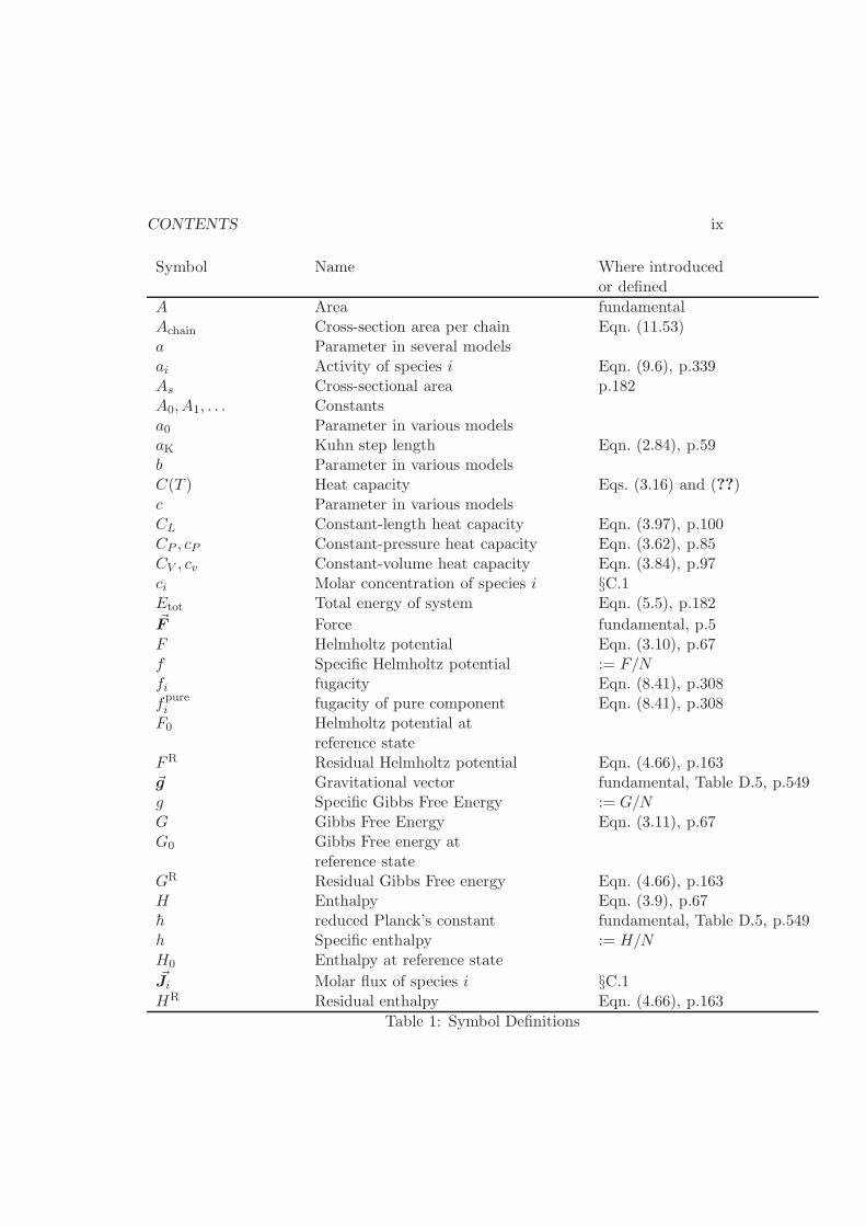
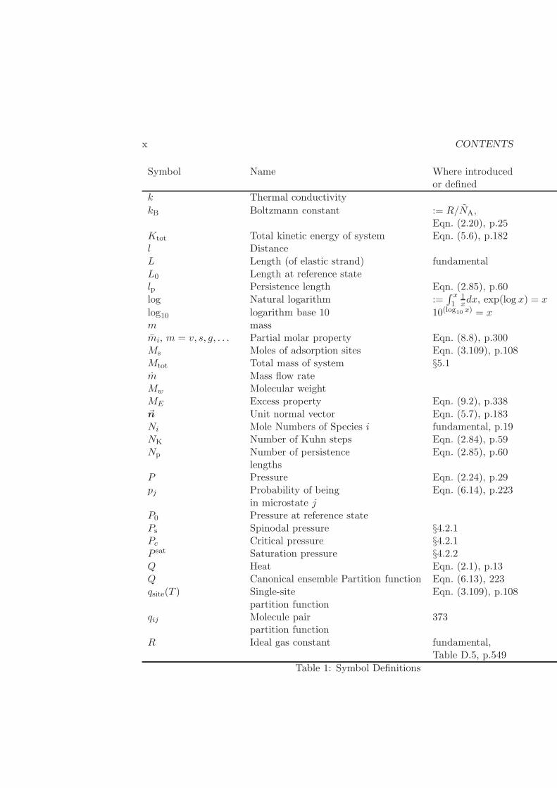
Symbol Name Where introducedor defined
A Area fundamentalAchain Cross-section area per chain Eqn. (11.53)a Parameter in several modelsai Activity of species i Eqn. (9.6), p.339As Cross-sectional area p.182A0, A1, . . . Constantsa0 Parameter in various modelsaK Kuhn step length Eqn. (2.84), p.59b Parameter in various modelsC(T ) Heat capacity Eqs. (3.16) and (??)c Parameter in various modelsCL Constant-length heat capacity Eqn. (3.97), p.100CP , cP Constant-pressure heat capacity Eqn. (3.62), p.85CV , cv Constant-volume heat capacity Eqn. (3.84), p.97ci Molar concentration of species i §C.1Etot Total energy of system Eqn. (5.5), p.182~F Force fundamental, p.5F Helmholtz potential Eqn. (3.10), p.67f Specific Helmholtz potential := F/Nfi fugacity Eqn. (8.41), p.308fpurei fugacity of pure component Eqn. (8.41), p.308F0 Helmholtz potential at
reference stateFR Residual Helmholtz potential Eqn. (4.66), p.163~g Gravitational vector fundamental, Table D.5, p.549g Specific Gibbs Free Energy := G/NG Gibbs Free Energy Eqn. (3.11), p.67G0 Gibbs Free energy at
reference stateGR Residual Gibbs Free energy Eqn. (4.66), p.163H Enthalpy Eqn. (3.9), p.67h reduced Planck’s constant fundamental, Table D.5, p.549h Specific enthalpy := H/NH0 Enthalpy at reference state~Ji Molar flux of species i §C.1HR Residual enthalpy Eqn. (4.66), p.163
Table 1: Symbol Definitions
x CONTENTS
Symbol Name Where introducedor defined
k Thermal conductivity
kB Boltzmann constant := R/NA,Eqn. (2.20), p.25
Ktot Total kinetic energy of system Eqn. (5.6), p.182l DistanceL Length (of elastic strand) fundamentalL0 Length at reference statelp Persistence length Eqn. (2.85), p.60log Natural logarithm :=
∫ x1
1xdx, exp(log x) = x
log10 logarithm base 10 10(log10 x) = xm massmi, m = v, s, g, . . . Partial molar property Eqn. (8.8), p.300Ms Moles of adsorption sites Eqn. (3.109), p.108Mtot Total mass of system §5.1m Mass flow rateMw Molecular weightME Excess property Eqn. (9.2), p.338~n Unit normal vector Eqn. (5.7), p.183Ni Mole Numbers of Species i fundamental, p.19NK Number of Kuhn steps Eqn. (2.84), p.59Np Number of persistence Eqn. (2.85), p.60
lengthsP Pressure Eqn. (2.24), p.29pj Probability of being Eqn. (6.14), p.223
in microstate jP0 Pressure at reference statePs Spinodal pressure §4.2.1Pc Critical pressure §4.2.1P sat Saturation pressure §4.2.2Q Heat Eqn. (2.1), p.13Q Canonical ensemble Partition function Eqn. (6.13), 223qsite(T ) Single-site Eqn. (3.109), p.108
partition functionqij Molecule pair 373
partition functionR Ideal gas constant fundamental,
Table D.5, p.549
Table 1: Symbol Definitions

CONTENTS xi
Symbol Name Where introducedor defined
r Number of species p.21Ri Reaction rate of species i §C.1S Entropy p.21, defined:
Eqn. (2.20), p.25s Specific entropy := S/NS0 Entropy at reference stateSR Residual entropy Eqn. (4.66), p.163Stot Total entropy of system Eqn. (5.10), p.184T Temperature Eqn. (2.25), p.29T0 Temperature at
reference stateTs Spinodal temperature §4.2.1Tc Critical temperature §4.2.1T Tension Eqn. (2.72), p.45U Internal Energy fundamental, p.11u Specific internal energy := U/NUj Energy of microstate j p.221U0 Internal energy at
reference stateUtot Total internal energy of system Eqn. (5.6), p.182UR Residual internal energy Eqn. (4.66), p.163V Volume fundamental, p.6v Specific volume := V/NV0 Volume at reference state~v Velocity := d~r/dt, p.5V R Residual volume Eqn. (4.66), p.163vc Critical volume §4.2.1vv Vapor volume §4.2.2vl Liquid volume §4.2.2v∞i Partial molar volume at infinite Eqn. (8.90)
dilution for species iW Work Eqn. (1.1), p.5X Unconstrained variable Eqn. (3.23), p.72z Compressibility factor Eqn. (4.28), p.144zc Critical compressibility factor §4.27∆gb Base pair denaturation Eqn. (3.102), p.103∆hb Base pair denaturation Eqn. (3.102), p.103
Table 1: Symbol Definitions
xii CONTENTS
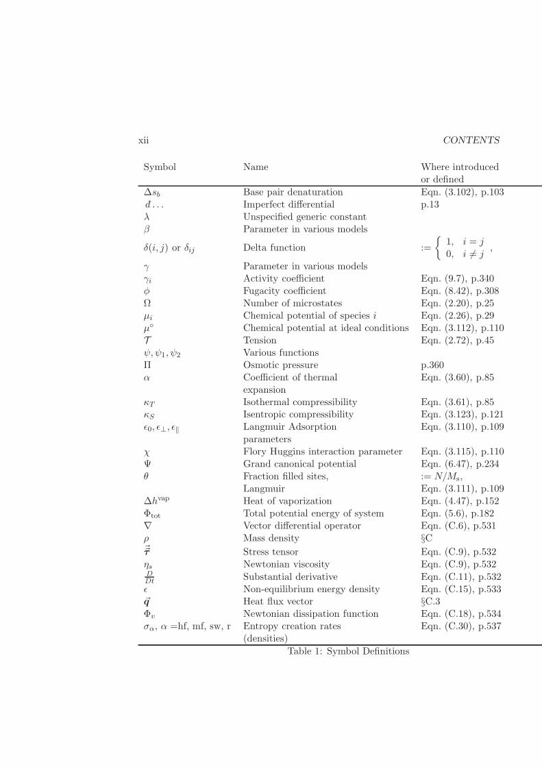
Symbol Name Where introducedor defined
∆sb Base pair denaturation Eqn. (3.102), p.103d . . . Imperfect differential p.13λ Unspecified generic constantβ Parameter in various models
δ(i, j) or δij Delta function :=
1, i = j0, i 6= j
,
γ Parameter in various modelsγi Activity coefficient Eqn. (9.7), p.340φ Fugacity coefficient Eqn. (8.42), p.308Ω Number of microstates Eqn. (2.20), p.25µi Chemical potential of species i Eqn. (2.26), p.29µ Chemical potential at ideal conditions Eqn. (3.112), p.110T Tension Eqn. (2.72), p.45ψ,ψ1, ψ2 Various functionsΠ Osmotic pressure p.360α Coefficient of thermal Eqn. (3.60), p.85
expansionκT Isothermal compressibility Eqn. (3.61), p.85κS Isentropic compressibility Eqn. (3.123), p.121ǫ0, ǫ⊥, ǫ‖ Langmuir Adsorption Eqn. (3.110), p.109
parametersχ Flory Huggins interaction parameter Eqn. (3.115), p.110Ψ Grand canonical potential Eqn. (6.47), p.234θ Fraction filled sites, := N/Ms,
Langmuir Eqn. (3.111), p.109∆hvap Heat of vaporization Eqn. (4.47), p.152Φtot Total potential energy of system Eqn. (5.6), p.182∇ Vector differential operator Eqn. (C.6), p.531ρ Mass density §C~~τ Stress tensor Eqn. (C.9), p.532ηs Newtonian viscosity Eqn. (C.9), p.532DDt Substantial derivative Eqn. (C.11), p.532ǫ Non-equilibrium energy density Eqn. (C.15), p.533~q Heat flux vector §C.3Φv Newtonian dissipation function Eqn. (C.18), p.534σα, α =hf, mf, sw, r Entropy creation rates Eqn. (C.30), p.537
(densities)
Table 1: Symbol Definitions
CONTENTS xiii
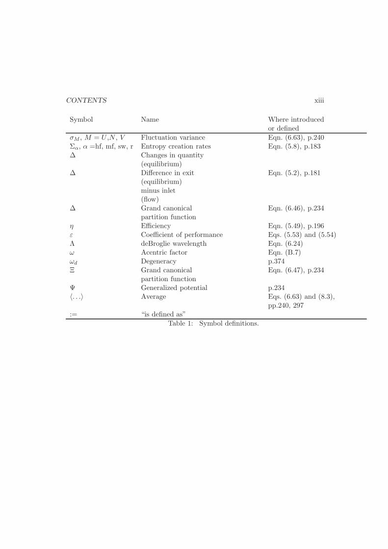
Symbol Name Where introducedor defined
σM , M = U ,N , V Fluctuation variance Eqn. (6.63), p.240Σα, α =hf, mf, sw, r Entropy creation rates Eqn. (5.8), p.183∆ Changes in quantity
(equilibrium)∆ Difference in exit Eqn. (5.2), p.181
(equilibrium)minus inlet(flow)
∆ Grand canonical Eqn. (6.46), p.234partition function
η Efficiency Eqn. (5.49), p.196ε Coefficient of performance Eqs. (5.53) and (5.54)Λ deBroglie wavelength Eqn. (6.24)ω Acentric factor Eqn. (B.7)ωd Degeneracy p.374Ξ Grand canonical Eqn. (6.47), p.234
partition functionΨ Generalized potential p.234〈. . .〉 Average Eqs. (6.63) and (8.3),
pp.240, 297:= “is defined as”
Table 1: Symbol definitions.
Chapter 1
Introduction
I wish to propose for the reader’s favorable considerationa doctrine which may, I fear, appear wildly paradoxical and
subversive. The doctrine in question is this: that it isundesirable to believe a proposition when there is no ground
whatever for supposing it true.
– Bertrand Russell1
For good or evil, all physical processes observed in the universe are subject tothe laws and limitations of thermodynamics. Since the fundamental laws of ther-modynamics are well understood, it is unnecessary to limit your own understandingof these thermodynamic restrictions.
In this text we lay out the straightforward foundation of thermodynamics, andapply it to systems of interest to engineers and scientists. Aside from consideringgases, liquids and their mixtures– traditional problems in engineering thermodynam-ics –we also consider the thermodynamics of DNA, proteins, polymers and surfaces.In contrast to the approach adopted by most traditional thermodynamics texts, webegin our exposition with the fundamental postulates of thermodynamics, and rig-orously derive all steps. When approximations are necessary, these are made clear.Therefore, the student will not only learn to solve some standard problems, but heor she will also know how to approach a new problem on safe ground before makingapproximations.
Thermodynamics gives interrelationships between the properties of matter. Of-tentimes these relationships are non-intuitive. For example, by measuring the vol-ume and heat capacity2 as functions of temperature and pressure, we can find all
1 “Introduction: On the Value of Scepticism,” Sceptical Essays (London, Allen & Unwin, 1928).2The heat capacity will be defined in Chapter 2, but roughly means something like the amount
1
2 CHAPTER 1. INTRODUCTION
other thermodynamic properties of a pure system. Then, we can use relations be-tween different thermodynamic properties to estimate the temperature rise of a fluidwhen it is expanded in an insulated container. Or, we can use such data to predictthe boiling point of a liquid. In Chapter 2, we introduce the necessary variables todescribe a system in thermodynamic equilibrium. We also discuss several assump-tions that are made early on. In that chapter, the natural thermodynamic variablesare energy and volume. Or, for a surface, energy and area, and for a polymer,energy and length. Subsequently, in Chapter 3, we introduce additional variablesthat are useful for solving problems when temperature and pressure are controlled.In Chapter 4, we consider phase diagrams for pure substances. In other words, welearn how to predict the temperature or pressure at which a pure liquid will boil, orwhen a pure vapor will condense.
Rigorously speaking, thermodynamics only applies to systems at equilibrium.That is, systems that are stable at rest, and that are not subject to a temperaturegradient or flow. However, for many systems out of equilibrium, it is possible tomake reasonable approximations and use thermodynamics even during flow, or whenthe temperature and pressure are changing with time. Such approximations areconsidered in Chapter 5, so that we may begin to solve problems involving flowsand changes.
Chapter 6 introduces statistical mechanics. Statistical mechanics allows us to(1) connect thermodynamics to molecular properties, (2) study small systems, andlarge systems near critical points, where thermodynamics does not apply, and (3)consider fluctuations in thermodynamic variables. Most of what follows in the bookdoes not require statistical mechanics, although the final section of most remainingchapters will invoke it.
In order to make a strong intuitive connection between molecules and thermody-namics, Chapter 7 discusses many of the important molecular interactions. Chapters8 and 9 introduce the machinery to solve vapor-liquid equilibrium problems, such asdew-point and bubble-point calculations, in mixtures. We study reactions in Chap-ter 10. Polymers and surfaces are considered throughout the text, but Chapters 11and 12 cover these topics in greater detail.
Thermodynamics is an extremely broad field, and no single text can cover all ofthe topics important to engineering and science. Therefore, it is usually importantto revisit thermodynamics repeatedly. In this book we try to give an overviewof many important topics in engineering, and a flavor of how these problems aresolved. Typically, more advanced models will exist to cover a given topic, but thesolution techniques are essentially the same. Let us consider some questions thatare appropriate to ask of the field. These are only representative of the very broad
of energy necessary to raise the temperature of a substance by one degree.
1.1. RELEVANT QUESTIONS FOR THERMODYNAMICS 3
scope of thermodynamics. Many more questions are possible than those presentedhere.
1.1 Relevant Questions for Thermodynamics
1. What is temperature? What does it have to do with ‘entropy’?
2. Pick up a butane lighter that has a transparent casing. Note that there is bothliquid and gas inside. These phases are both butane at the same temperatureand pressure. Yet, some of it is liquid and the rest is gas. Why? How can wepredict when the substance will be just one phase, and when it will separateinto two? (See an example of a region where a model fluid makes two phases—called a phase diagram—in Fig.4.5 on p.148.)
3. Press the button to open the valve in the lighter, but without striking theflint to start a flame, and measure the temperature of the exiting fluid. It isapproximately the temperature of an ice cube. Could we have predicted that?
4. A refrigerator (or air conditioner) makes heat flow from a cold space to a warmone. How does it do that? How much energy must we expect to buy from theutility company to do that?
5. Compress an ideal gas (say air in a balloon) at constant temperature. Theballoon pushes back, so it can be used to do work, say lift a book off of thefloor. However, it is possible to prove that the compressed and uncompressedgas has the same energy. So, how can it do work? A traveling gypsy told methat energy is ‘the ability to do work’. Was he wrong?
6. Stretch a rubber band and move it quickly to your lips; it feels warm. Let itcontract, and it feels cool. Why does a rubber band do that? It is also anexperimental fact that a rubber band’s tension at constant length increaseswith temperature, as can be shown with a hair dryer. That is not true for ametal spring. It certainly does not seem obvious that these observations arerelated—could thermodynamics tell us why?
7. Some pure-component fluids, or mixtures of fluids, refract white light in beau-tiful, opalescent ways, showing many colors. This thermodynamic point (spe-cific temperature, density, etc.) is called the critical point . How do these fluidsdo that?
8. Creutzfeldt-Jakob disease was initially transmitted from one surgery patientto another by surgical tools, although the tools had supposedly been sterilized
4 CHAPTER 1. INTRODUCTION
by heat. Many researchers now believe that the disease is not caused by anorganism, but by an errant protein called a prion. How can a single errantprotein out of countless in the brain cause such a degenerative disease?
9. We have all learned that ‘like likes like’, e.g., olive oil dissolves in vegetableoil, but not in water. What is the explanation for this?
10. Contrary to the previous statement, polymers do not easily dissolve in solventsof similar chemical makeup, and do not mix with nearly identical polymers. Infact, Fig.11.3 on p.440 shows that a mixture of hydrogenated and deuteratedpolybutadiene are not miscible, although they are chemically nearly identical!Why?
11. We learn early in physics that energy is conserved. Yet, most economic anal-yses revolve around the cost of energy. If it is always around, why are we soconcerned with it?
12. Mechanical laws allow for the existence of a perpetual motion device. How dothe laws of thermodynamics prohibit its existence?
13. Air flows into the Ranque-Hilsch vortex tube of Figure 5.3 on p.191 at roomtemperature, but exits in a hot stream and a cold stream. Although energyis conserved, it seems like we are getting a free lunch. How is this physicallypossible? Couldn’t we build a perpetual motion machine from it?
14. Certain molecules in a gas phase can react only when they are adsorbed ona catalytic surface. If we increase the pressure in the gas phase, how will theamount of adsorption change? How is it that some people use this experimentto estimate surface area in porous materials?
15. If the pressure ‘acting’ on a substance is increased at constant temperature,will its volume always decrease?
16. If your equipment tells you that the heat capacity of your new wonder com-pound is negative, is it time to call technical support for the manufacturer?
17. We find that the ground water for our drinking supply has been contaminated.How much energy must we expend to remove the contaminant?
18. What is the best separation we can expect from distillation? What is theminimum amount of energy necessary to achieve this separation?
19. If we burn one gallon of gasoline, what is the most amount of work we canexpect to get out?
1.2. WORK AND ENERGY 5
20. In primary school, I learned that there were three phases of matter: gas, liquidand solid. This is incorrect. What other kinds of phases are there?
21. Someone once told me that a fuel cell has a higher theoretical efficiency thanan engine. Is that true?
22. If one uses optical tweezers to pull on a segment of DNA, why does the strandpull back?
23. A helical coil of DNA in a solvent will uncoil, and separate into two strands ifthe temperature is raised—so called, denaturing . Actually, there is a range oftemperatures where the DNA is partially coiled and attached, and partiallyseparated. What is this temperature range, and how does it change withsolvent?
The following chapters should help you answer all of these questions. For themoment, let us review a couple of basic concepts that are important to begin.
1.2 Work and Energy
The mathematics background necessary to follow this book is reviewed in AppendixA. We assume that the reader is familiar with the typical units and dimensions oflength, mass, and energy. Work and energy play key roles in thermodynamics, solet us review these physical concepts briefly.
Recall that work is defined as force times distance3
Work := Force ×Distance. (1.1)
If I lift an object of mass m off the floor a distance l, then the work I have done onthe object is the constant force m~g, times the distance l. Hence, W = m|~g|l, where|~g| is the gravitational constant, and W is work.
We also know that energy is conserved, so that the potential energy Epotential ofthe object must have increased, ∆Epotential := Efinal
potential − Einitialpotential = m|~g|l.
By similar arguments, we can find other forms of energy, such as kinetic energy.For example, if we exert a constant force ~F on a baseball of mass m, neglectingfriction with air, the ball will undergo constant acceleration according to Newton’sclassical mechanics
~F = md~v
dt, (1.2)
3The symbol := means ‘is defined as’.
6 CHAPTER 1. INTRODUCTION
where ~v is the velocity of the ball, and t is time. During an infinitesimal time dt,the ball is displaced ~vdt. Hence, the infinitesimal change in kinetic energy of theball Ekinetic is the infinitesimal amount of work
dEkinetic = ~F · ~vdt = md~v
dt· ~vdt = m~v · d~v. (1.3)
If we integrate each side from zero initial speed (and zero kinetic energy), to thefinal speed |~v|, we find
Ekinetic =1
2m|~v|2. (1.4)
We see that if we know the force and displacement of an object, we can find itschange in kinetic energy. You may already be familiar with the result, but noticehow it was obtained—from the definition of work, and the conservation of energy.Similar ideas will be used in Chapter 2.
Note that power is the rate at which we do work. Hence, the quantity ~F · ~v isthe power exerted on the ball.
Example 1.2.1 A piston in a box changes the volume V in the box. How muchwork does it take to compress the piston a distance L?
Solution: Since the pressure P might change inside the box by the actof compression, it is best to begin with an infinitesimal compression of thepiston. The infinitesimal work (∆W ) is the force times the infinitesimal distance(∆Distance) the piston moves. However, the force is the pressure times the areaA of the piston
∆W = PA∆Distance = −P∆V. (1.5)
where ∆V is the change in volume of the box. Make careful note of the minussign. If we integrate all of these infinitesimal changes, we obtain
W = −∫ Vf
V0
PdV, (1.6)
where V0 and Vf are the initial and final volumes of the box.We can test our answer by examining the dimensions. Work has units of en-
ergy. Potential energy is m|~g|l, so it has units of (mass×length2/time2), since|~g| has dimensions of acceleration. The integral on the right side has dimensionsof pressure times volume. Pressure is (force/area), or (mass×length/time2/length2),or (mass/time2/length). Hence, the integral has dimensions (mass×length2/time2)and our analysis is dimensionally consistent. 2
In the previous example, we found the work done to compress a gas in a box.But what form of energy changed? Is there an additional way to change this formof energy? The answers to these questions are given in Chapter 2.
1.3. EXERCISES 7
1.3 Exercises
1.1.A. By searching other texts, find examples of problems where thermodynamicsplays an important role in understanding. Cite your reference(s). (Actually, it wouldbe much more difficult to find a problem where thermodynamics does not apply.)
1.1.B. In later chapters (§3.6) we discover that all thermodynamic properties can bereduced to just a few measurable quantities. Two of these quantities are called ‘thecoefficient of thermal expansion’, defined by Eqn. (3.60), and ‘the isothermal com-pressibility,’ Eqn. (3.61). Design simple experiments to measure these two quantitiesfor a substance. Although it has not yet been introduced, assume that temperatureis easily measured by a thermocouple, whose probe is a thin wire.
1.1.C. Aside from gas, liquid and solid, what other kinds of phases are there? Thereare actually several kinds of solid phases, so you may choose to name and describeone of these. Please give a reference from which you learned of this phase of matter.The more obscure and bizarre the phase is, the better.
1.2.A. If we exert a torque Tω on a stirring paddle such that it rotates with angularvelocity ω, how much power (work per time) are we exerting on the paddle?
1.2.B. What other kinds of energy can you think of? Cite some examples wheresuch forms might be relevant, and how it might inter-convert with some other formof energy.
1.2.C. How much work does it take to stretch a spring from a length L0 to L if youknow how the tension T varies with L? In particular, what if the tension is zero atL0, and varies linearly with displacement?
1.2.D. A lever arm allows one to exert large forces. In other words, one gives asmall force at one end of the arm, and a large force is given by the end nearer thefulcrum. Is work ‘conserved’ in this case? In other words, does the lever arm exertthe same work at the short end that it receives at the long end? Show your answerquantitatively.

8 CHAPTER 1. INTRODUCTION

Chapter 2
The Postulates ofThermodynamics
So, as science has progressed, it has been necessary toinvent other forms of energy, and indeed an unfriendly
critic might claim, with some reason, that the law ofconservation of energy is true because we make it trueby assuming the existence of forms of energy for whichthere is no other justification than the desire to retain
energy as a conservative quantity.
– Kenneth S. Pitzer [69].
Thermodynamics is the combination of a structure plus an underlying governingequation. Before designing plays in basketball or volleyball, we first need to laydown the rules to the game—or the structure. Once the structure is in place, wecan design an infinite variety of plays, and ways that the game can run. Some ofthese plays will be more successful than others, but all of them should fit the rules.Of course, in sports you can sometimes get away with breaking the rules, but MotherNature is not so lax. You might be able to convince your boss to fund constructionof a perpetual motion machine, but the machine will never work.
In this chapter we lay the foundation for the entire structure of thermodynamics.Remarkably, the structure is simple, yet powerfully predictive. The cost for suchelegance and power, however, is that we must begin somewhat abstractly. We needto begin with two concepts: energy and entropy. While most of us feel comfort-able and are familiar with energy, entropy might be new. However, entropy is nomore abstract than energy—perhaps less so—and the approach we take allows usto become as skilled at manipulating the concept of entropy as we are at thinking
9
10 CHAPTER 2. THE POSTULATES OF THERMODYNAMICS
about energy. Therefore, in order to gain these skills we consider many exampleswhere an underlying governing equation is specified. For example, we consider thefundamental relations that lead to the ideal gas law, the van der Waals equation ofstate, and more sophisticated equations of state that interrelate pressure, volumeand temperature.
Although the postulates are fairly simple, their meaning might be difficult tograsp at first. In fact, most students will need to revisit the postulates many times,perhaps over several years. We recommend that you think about the postulates theway you might vote in Chicago—early and often (or even after you die). Throughoutmost of the book, however, we will use the postulates only indirectly; in other words,we will derive some important results in this chapter, and then use these resultsthroughout the book. It is therefore important to remember the results derivedhere, and summarized at the end of the chapter.
2.1 The Postulational Approach
Where does Newton’s law of motion ~F = ddt(m~v) come from? Where did Einstein
discover E = mc2? These equations were not derived from something—they wereguessed in a flash of brilliant insight. We have come to accept them for a few reasons:First, because they describe a great many experiments, and were used to predictpreviously unknown phenomena. Secondly, they are simple and straightforwardto comprehend, although perhaps sometimes difficult to implement. Thirdly, andmore importantly, we accept these assertions, or postulates, of Newton and Einsteinbecause we have never seen them violated. It is for these reasons—despite Pitzer’s‘unfriendly critic’—that we believe that energy is always conserved.
In this chapter we describe the postulates that make up the theory of thermody-namics. Just like Newton and Einstein, we must be willing to abandon our theoryif experiments ever contradict the postulates. The postulates given here are not themost general possible, but are designed to be easily understood, and applicable tomost systems of interest to engineers and scientists. In a few sections we brieflyconsider generalizations. The approach in this chapter is essentially that of Callen[13]. Hence, the same restrictions apply—namely, the system must be isotropic, ho-mogeneous, large enough to neglect surface effects if we are talking about the bulk,or that we may neglect edge effects if we are talking about surfaces, and no externalforces.
In what follows we make five fundamental postulates. The first postulate (firstlaw) posits the existence of an additional form of energy called ‘internal energy’,which, along with kinetic, potential, electromagnetic and other energies, obeys aconservation principle. The second postulate assumes that every system has equilib-

2.2. THE FIRST LAW: ENERGY CONSERVATION 11
rium states that are determined by a few macroscopic variables. The third postulateintroduces a quantity called ‘entropy’ on which internal energy depends. The fourthpostulate (the second law) and the fifth (Nernst) postulate prescribe properties ofentropy. The rest of thermodynamics follows from these straightforward ideas tohave far-reaching consequences.
2.2 The First Law: Energy Conservation
What is the definition of energy? Despite using the word and the concept nearly ev-eryday, most engineers and scientists stop short when asked this question. Nonethe-less, we still find the concept very useful. Consider a few simple thought experimentsabout energy. (1) How much energy does this book have if you hold it above yourhead before letting it drop to the floor? You might answer that it has potentialenergy m|~g|l, where |~g| is the gravitational constant, and l is the height of the bookabove the floor. (2) If the book is flying with speed |~v| while it is height l above thefloor, is its energy m|~g|l+ 1
2m|~v|2? (3) What if I place an ice cube on the book? Wenote that the ice melts, and we assume (correctly) that heat was transferred fromthe book to the ice.
What do these experiments tell us? First, we notice that the energy we ascribedto the book changed depending on the situation. That is because the situationsmade us think about several different degrees of freedom or variables that we usedto define the book’s energy. When we held the book over our head, we instinctivelythought of position, and then calculated the potential energy of the book. When wepictured the book flying, we then thought of position and velocity, and added thekinetic energy. When the ice melted on the book, we thought about concepts liketemperature, heat, or maybe internal energy.1
Note that before we can talk about energy accurately, it is important to specifythe system, and to specify what variables we are using . In our first example thesystem is the book, and the position of the book is the variable. The other importantpoint is the first law, or first postulate:
Postulate I (First Law): Macroscopic systems possess an internal energyU that is subject to a conservation principle, and is extensive.
An extensive variable is one that is linearly dependent on system size, andconversely, an intensive variable is one that is independent of system size.2 From
1Our postulates will allow us to distinguish clearly between internal energy, heat and tempera-ture.
2A precise mathematical definition will be given shortly, in Postulate III.
12 CHAPTER 2. THE POSTULATES OF THERMODYNAMICS
a statistical mechanical, or atomistic point of view, we do not need this postulate,since we know that atoms store energy. We also know that all forms of energy areconserved. However, we choose to make this starting point clear in our frameworkby making it as a postulate.
This internal energy is somehow transferred from the book to the ice in ourthought experiment. Internal energy has properties just like other forms of energyin that it can be exchanged between different systems, convert to and from otherforms of energy, or be used to extract work. By ‘conservation principle,’ we meanthat if we add up all of the forms of energy in an isolated system, the sum total ofthose energies is constant, although one form might have increased while anotherdecreased, say some kinetic energy became internal energy. It is worthwhile to quoteextensively from Callen [13, p.11].
The development of the principle of conservation of energy has been oneof the most significant achievements in the evolution of physics. Thepresent form of the principle was not discovered in one magnificent strokeof insight but was slowly and laboriously developed over two and a halfcenturies. The first recognition of a conservation principle repeatedlyfailed, but in each case it was found possible to revive it by the addition ofa new mathematical term—a “new kind of energy.” Thus considerationof charged systems necessitated the addition of the Coulomb interactionenergy (Q1Q2/r) and eventually of the energy of the electromagneticfield. In 1905 Einstein extended the principle to the relativistic region,adding such terms as the relativistic rest-mass energy. In the 1930s En-rico Fermi postulated the existence of a new particle called the neutrinosolely for the purpose of retaining the energy conservation principle innuclear reactions . . . .
Where is internal energy stored? Although it is not necessary to introduce atomsand molecules into the classical theory of thermodynamics, we might be bothered bythis question. The answer might be in the vibrations of the atoms (kinetic energy)and the spring-like forces between atoms (potential energy), or in the energies inthe subatomic particles. So why do we call it ‘internal energy’ instead of kinetic+ potential energy, for example? Recall our thought experiments above, where wefound that the variables used to describe our system are essential to define energy. Ifwe knew the precise positions and velocities of all the atoms in the book, we could,in principle, calculate all ∼ 1023 kinetic and potential energies of the book, andwe would not need to think about internal energy. However, that approach is notonly impractical, but, it turns out, is not even necessary. We can make meaningfulcalculations of internal energy by using just a few variables that are introduced inPostulate III.

2.3. DEFINITION OF HEAT 13
2.3 Definition of Heat
If we do work on a system, then its energy must be increased. However, we oftenobserve that after we do work on a system, its internal energy returns to its originalstate, although the system has done no work on its environment. For example, pushthe book across the table, then wait a few minutes. Although you performed workon the book, it has the same initial and final potential, kinetic and internal energies.The reason the internal energy of a system can change without work is that energycan also be transferred in the form of heat.
Since the internal energy of a system may be changed either by work, or by heattransfer, and we have postulated that energy is conserved, we can define the heattransfer to, or from, a system as
dQ := dU − dW. (2.1)
It is worthwhile to commit this equation to memory, or better yet: dU = dQ+dW . In this notation, work is positive when done on the system, and heat is positivewhen transferred to the system. We write the differentials for heat and work usingd instead of d because they are imperfect differentials.
Perfect differentials are not dependent upon the path taken from the ‘ini-tial’ to the ‘final’ states—they only depend on the initial and final values ofthe independent variables. Imperfect differentials d have two importantproperties that distinguish them from perfect differentials d. First, imperfectdifferentials do depend upon the path. For example, if we set this book onthe floor and push it a short distance d~x away using force ~F and then thesame distance −d~x back to its original position using force − ~F , then the sum(perfect) differential for its position is zero—exactly the same as if we had leftthe book sitting there: d~xtot = d~x1 + d~x2 = d~x + (−d~x) = 0. However, thework done on the book was positive in both moves, so the sum (imperfect)differential of the work is positive, even though the book ended up where itbegan: dWtot = ~F1 · d~x1 + ~F2 · d~x2 = ~F · d~x+ (− ~F ) · (−d~x) = 2 ~F · d~x.Second, if we integrate a perfect differential, we obtain a difference betweenfinal and initial states. For example, if we integrate d~x from ~x0 to ~x1, weobtain the difference ∆~x = ~x1 − ~x0. When we integrate dW , for example,we simply obtain the total work in the path W , not a difference.
In order to control, and therefore measure, the internal energy of a system, weneed to control both the heat flow and the work done on the system. This ma-nipulation is accomplished primarily through control of the walls of a system. The
14 CHAPTER 2. THE POSTULATES OF THERMODYNAMICS
following definitions establish ideal conditions that we may approach approximatelyin real situations.
An adiabatic wall is one that does not allow heat to flow through it. In realsituations this is approximated by heavily insulated walls. On the other hand, adiathermal wall is one that permits heat to flow through it freely. In addition, weoften assume that the wall has a sufficiently small mass such that its thermodynamiceffects are negligible. Such a wall might be approximated by one that is thin, andmade of metal.
When no matter is exchanged with the environment, we say the system is closed.When no mass, heat, or work is exchanged, we say the system is isolated. Whenboth energy and mass can be exchanged, we say that the system is open.
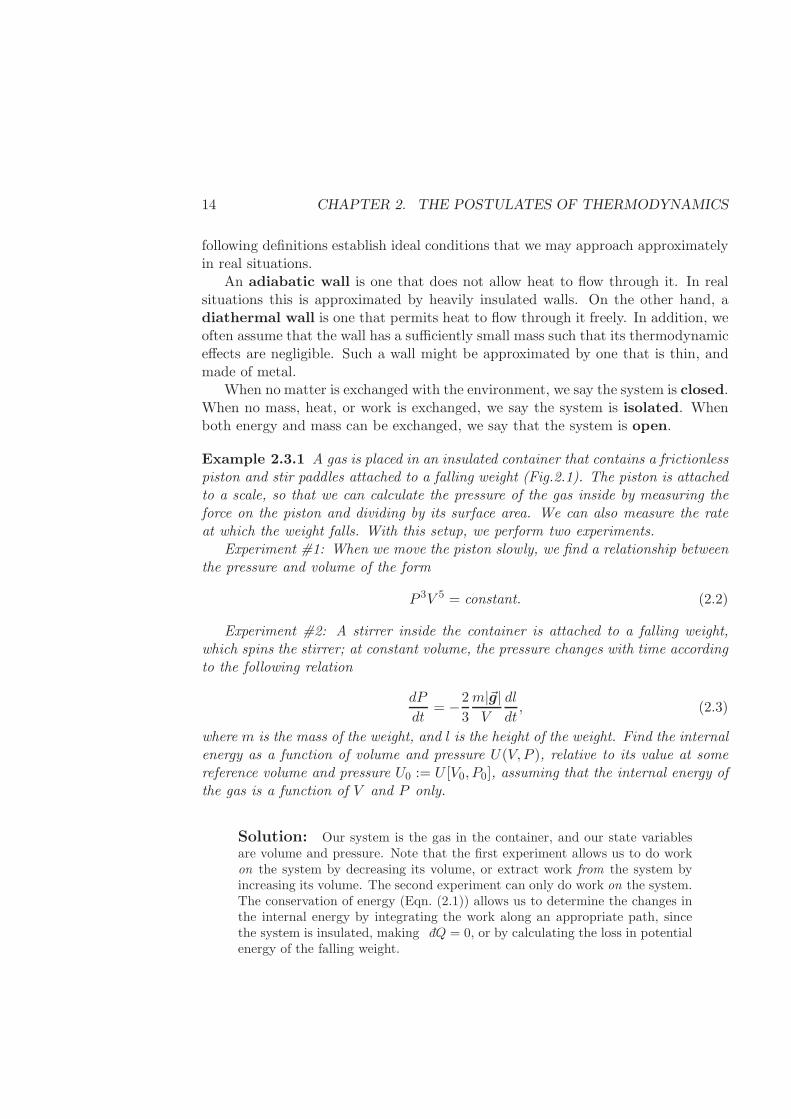
Example 2.3.1 A gas is placed in an insulated container that contains a frictionlesspiston and stir paddles attached to a falling weight (Fig.2.1). The piston is attachedto a scale, so that we can calculate the pressure of the gas inside by measuring theforce on the piston and dividing by its surface area. We can also measure the rateat which the weight falls. With this setup, we perform two experiments.
Experiment #1: When we move the piston slowly, we find a relationship betweenthe pressure and volume of the form
P 3V 5 = constant. (2.2)
Experiment #2: A stirrer inside the container is attached to a falling weight,which spins the stirrer; at constant volume, the pressure changes with time accordingto the following relation
dP
dt= −2
3
m|~g|V
dl
dt, (2.3)
where m is the mass of the weight, and l is the height of the weight. Find the internalenergy as a function of volume and pressure U(V, P ), relative to its value at somereference volume and pressure U0 := U [V0, P0], assuming that the internal energy ofthe gas is a function of V and P only.
Solution: Our system is the gas in the container, and our state variablesare volume and pressure. Note that the first experiment allows us to do workon the system by decreasing its volume, or extract work from the system byincreasing its volume. The second experiment can only do work on the system.The conservation of energy (Eqn. (2.1)) allows us to determine the changes inthe internal energy by integrating the work along an appropriate path, sincethe system is insulated, making dQ = 0, or by calculating the loss in potentialenergy of the falling weight.
2.3. DEFINITION OF HEAT 15
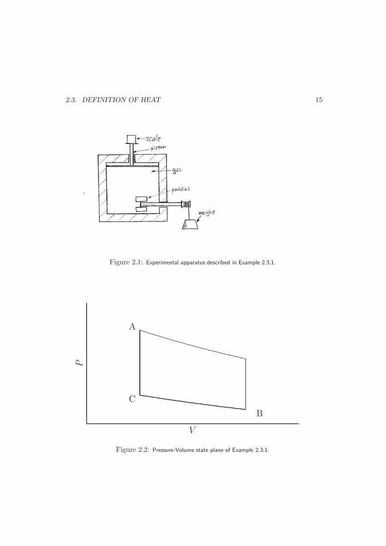
Figure 2.1: Experimental apparatus described in Example 2.3.1.
C
A
B
V
P
Figure 2.2: Pressure-Volume state plane of Example 2.3.1.

16 CHAPTER 2. THE POSTULATES OF THERMODYNAMICS
If we consider the state of the system on a plane with volume as the x axisand pressure as the y axis, then we see that each experiment allows us to movein the plane only in a specific manner. If the system begins at a specific pressureand volume, then the second experiment allows us to increase the pressure, butnot change the volume. The first experiment allows us to change both thepressure and the volume, but only such that P 3V 5 stays constant. However,these two experiments are sufficient to allow us to move on the state planebetween any two points.
For example, the points A and B in Figure 2.2 can be connected by twodifferent paths. First, we can draw a vertical line through point A indicatingthe second experiment, and a line of constant P 3V 5 through point B, indicatingthe first experiment. We can then proceed along the path using the two linesegments that connect these two points. Alternatively, we could draw a verticalline through point B and a line of constant P 3V 5 through point A and connectthe points. Once we have a path connecting the points, we integrate the workrequired to move between them. Consider the first path.
Since the point C is connected to point A by Experiment #2 and to pointB by Experiment #1, its pressure and volume must satisfy the two equations
VA = VC (2.4)
P 3CV
5C = P 3
BV5B .
From which we may readily solve for PC
PC = PB
(VBVA
)5/3
. (2.5)
Similarly, for any point on the line connecting B and C, the pressure can befound as a function of volume
P (V ) = PB
(VBV
)5/3
, curve connecting B and C. (2.6)
Since Experiment #1 is performed quasi-statically, we can assume that thepressure in the container is that measured on the piston. Therefore, Eqn. (2.1)can be written as
dU = dWqs
= −PdV. (2.7)
Using Eqn. (2.6) we obtain
dU = −PB
(VBV
)5/3
dV. (2.8)
We can integrate Eqn. (2.8) from C to B to obtain
U [VB, PB]− U [VC, PC] = −3
2PBVB
[(VBVA
)2/3
− 1
]
. (2.9)
2.3. DEFINITION OF HEAT 17
Note that we use the square brackets [. . .] to indicate where the quantity is beingevaluated, as opposed to parentheses (. . .) to indicate a functional dependence.For example, we would write U(V, P ) to indicate that U depends upon V andP , and U [PA] to indicate that we are evaluating U at PA, but arbitrary V .
To integrate U along path CA, we need to find the work done during theexperiment. Recalling that the potential energy of the weight is m|~g|l andneglecting any kinetic energy of the falling weight, an energy balance on thecontainer plus weight yields: d(U +m|~g|l) = 0. We can therefore write
dU = −m|~g|l dt
=3
2V dP, (2.10)
where we have used Eqn. (2.3) to obtain the second line. Since the volume isconstant along CA, we can integrate Eqn. (2.10) from C to A to give
U [VA, PA]− U [VC, PC] =3
2VA(PA − PC)
=3
2VA
[
PA − PB
(VBVA
)5/3]
, (2.11)
where we have used Eqn. (2.5). Let us call A our reference state: (PA, VA) →(P0, V0), and let B be any arbitrary state: (PB, VB) → (P, V ). If we subtractEqn. (2.11) from Eqn. (2.9), we obtain our desired expression for the internalenergy of the system
U(V, P )− U0 =3
2(PV − P0V0) (2.12)
Equation (2.12) is an example of an equation of state—an equation thatrelates several thermodynamic properties with one another. Another exampleis the well-known ideal-gas equation of state (Pv = RT ) that relates pressure,volume and temperature with one another. 2
The equation of state derived in Example 2.3.1 is used in the following exampleto calculate heat flows in a system.
Example 2.3.2 The gas from Example 2.3.1 is placed in a container with a diather-mal wall and a frictionless piston. Find the amount of heat and work necessary fortwo different steps: The first step decreases the pressure from P1 to P2 at constantvolume V1. The second process increases the volume from V1 to V2 at constantpressure P2. Assume each step is quasi-static.
Solution: In the first step, the volume is held constant, so dV = 0, and theamount of work done on the system is zero: W I = 0. Therefore, the definitionfor heat flux Eqn. (2.1) becomes
dQ = dU, (2.13)

18 CHAPTER 2. THE POSTULATES OF THERMODYNAMICS
which we can integrate along any path from the initial (P1, V1) to the final(P2, V1) conditions to give
QI =
∫ (P2,V1)
(P1,V1)
dU(P, V )
= U [P2, V1]− U [P1, V1]
=3
2V1 (P2 − P1) . (2.14)
The third line follows from Eqn. (2.12). Since P1 > P2, then QI < 0. Toperform this step, we must extract heat from the system.
In the second step, the volume changes, so work is done. If we integrateEqn. (2.1) over the second step (P2, V1) → (P2, V2), we obtain
QII =
∫ V2
V1
P2dV +
∫ V2
V1
dU [V, P2]
= P2
∫ V2
V1
dV + U [V2, P2]− U [V1, P2]
= P2 (V2 − V1) +3
2P2 (V2 − V1)
=5
2P2 (V2 − V1) . (2.15)
Note that the first term on the right-hand side of the third line of Eqn. (2.15)represents the work done in the second step: W II = P2 (V2 − V1). 2
Here we have used straightforward experiments to find heat exchanges for asystem, and how the internal energy depends on pressure and volume. Then weused these results to predict how to manipulate the system in a desired way. InExample 2.6.2 we give the complete characterization of this fluid, which is called asimple, ideal gas. At low densities, all gases behave ideally; later we will see thatsimple gases are mono-atomic. At higher densities, more complicated equations ofstate are necessary to accurately describe the behavior of liquids and gases. Severalof these are given in the appendix, and we will call on them throughout the book.
2.4 Equilibrium States
The density of pure water at 1 atm and 25C is always 1 g/cm3, no matter wherethe water comes from. This observation holds if I start with ice from Lake Mendotain the winter, or with steam from a teapot in Shanghai. We call this stable state ofwater an equilibrium state. Thermodynamics deals only with these equilibriumstates, and not with the dynamics of the system between such states. (However,
2.5. ENTROPY, THE SECONDLAW, AND THE FUNDAMENTAL RELATION 19
it does tell us which equilibrium states are available to a system that is not atequilibrium, and which states are not.) Thermodynamics just does not say howlong, or by what path the system will attain equilibrium. These observations leadus to the second, rather sensible postulate.
Postulate II: There exist equilibrium states of a macroscopic system thatare characterized completely by the internal energy U , the volume V , and themole numbers of the m species N1, N2, . . . , Nm in the system.
If we know U , the volume and the mole numbers, then the equilibrium state isfixed.
When we do work on a system, we often wish to consider processes that occurslowly. In such a case, we assume that the system is nearly always in an equilibriumstate. We call such a slow change a quasi-static process. For example, we mightchange the pressure in a container by changing the force on a piston slowly, perhapsby removing grains of sand that are resting on the piston one at a time. When wechanged the pressure slowly in Example 2.3.1, we were changing it quasi-statically.
2.5 Entropy, the Second Law, and the Fundamental Re-
lation
Since we do not have information on the positions and velocities of all of the atoms,we need to determine what set of variables is necessary to describe the internalenergy of our system. A few observations can guide us:
• When touching a hot stove, we notice that it transfers some internal energyto us (don’t try this experiment at home without the supervision of an adult).Intuitively we know that this mechanism of energy storage has something todo with temperature and heat flow.
• In order to make an air balloon smaller, we have to do work on the balloonby squeezing it. This mechanism has something to do with applied force andvolume.
• To place more air molecules in the balloon, we do work on the balloon byblowing, or pumping. This mechanism has something to do with the numberof moles of gas in the balloon.
Our observations have suggested a number of possible independent variables forthe internal energy: one involving heat or temperature, a second involving volume or
20 CHAPTER 2. THE POSTULATES OF THERMODYNAMICS
pressure, and a third involving mole number. We do not wish to use heat, however,since it is handled using an imperfect differential. When a system is changed quasi-statically, then the work described in the second bullet above can be written asdW = −PdV . We need to introduce a second quantity called entropy that willallow us to use only perfect differentials for changes to U from heat flow.
We save time and effort by jumping directly to the correct answer. The justifi-cation for these choices will have to come from the ability of the theory to explainexperimentally observed phenomena.
At this point it is instructive to digress momentarily and elaborate on some ofthe underlying mathematical ideas behind our next postulate. Generally speaking,when facing a complex problem involving multiple variables, a common strategyis to define an objective function that one tries to maximize or minimize subjectto several constraints until a solution is found. As an example, a city might wantto alleviate congestion by controlling the size of the streets, the location of trafficlights, the duration and sequence of green lights, etc. To do so, city planners mightconstruct an objective function that they might chose to maximize or minimize. Anumber of choices are possible; a reasonable possibility could be to create a functionthat describes the average idle time per driver. Mathematically speaking, idle timewould be a function of the variables listed above. For a given number of cars or “flowrate”and a given street layout, one would then attempt to minimize that function bycontrolling the arrangement of traffic lights. Thermodynamics does the same thing;a function of several “natural variables”, such as the volume and the size of thesystem, is created and maximized or minimized (depending on the nature of thatfunction). One difference is that nature seems to have already chosen the functionthat is to be maximized. That function must meet several criteria, which is reallywhat the next postulate is about.
2.5. ENTROPY, THE SECONDLAW, AND THE FUNDAMENTAL RELATION 21
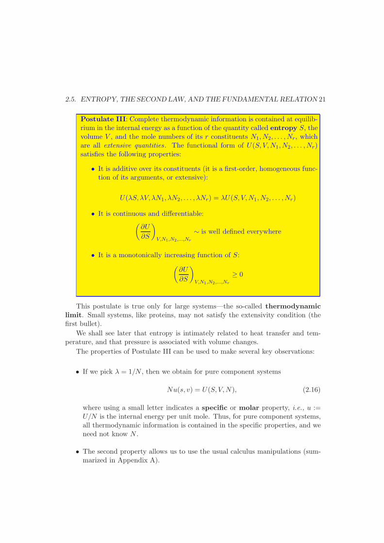
Postulate III: Complete thermodynamic information is contained at equilib-rium in the internal energy as a function of the quantity called entropy S, thevolume V , and the mole numbers of its r constituents N1, N2, . . . , Nr, whichare all extensive quantities. The functional form of U(S, V,N1, N2, . . . , Nr)satisfies the following properties:
• It is additive over its constituents (it is a first-order, homogeneous func-tion of its arguments, or extensive):
U(λS, λV, λN1, λN2, . . . , λNr) = λU(S, V,N1, N2, . . . , Nr)
• It is continuous and differentiable:(∂U
∂S
)
V,N1,N2,...,Nr
∼ is well defined everywhere
• It is a monotonically increasing function of S:
(∂U
∂S
)
V,N1,N2,...,Nr
≥ 0
This postulate is true only for large systems—the so-called thermodynamiclimit. Small systems, like proteins, may not satisfy the extensivity condition (thefirst bullet).
We shall see later that entropy is intimately related to heat transfer and tem-perature, and that pressure is associated with volume changes.
The properties of Postulate III can be used to make several key observations:
• If we pick λ = 1/N , then we obtain for pure component systems
Nu(s, v) = U(S, V,N), (2.16)
where using a small letter indicates a specific or molar property, i.e., u :=U/N is the internal energy per unit mole. Thus, for pure component systems,all thermodynamic information is contained in the specific properties, and weneed not know N .
• The second property allows us to use the usual calculus manipulations (sum-marized in Appendix A).
22 CHAPTER 2. THE POSTULATES OF THERMODYNAMICS
• The second and third properties allow us to invert the relation U = U(S, V ,N1, . . ., Nr) to find a unique function for S
S = S(U, V,N1, . . . , Nr), (2.17)
which enjoys properties similar to those enjoyed by U . Namely, we can writethat (
∂S
∂U
)
V,N1,...,Nr
> 0, and is well defined. (2.18)
Property (2.18) follows from Eqn. (A.18).
• Since we can invert U to find an expression for S, we can also show that S isa homogeneous, first-order function of its arguments
S(λU, λV, λN1, λN2, . . . , λNr) = λS(U, V,N1, N2, . . . , Nr). (2.19)
Therefore, we may deal either with S, or with U as the dependent variable.The appropriate choice is only dictated by convenience; there is no more infor-mation in U(S, V,N1, . . . , Nr) than there is in S(U, V,N1, . . . , Nr). The firstform is called the fundamental energy relation, and the second is calledthe fundamental entropy relation. These are sometimes called constitu-tive relations, since different fundamental relations often exist to describe asingle substance. For example, to describe oxygen we might sometimes use anideal gas (at low densities), a virial relation (at moderate densities), or a Peng-Robinson relation (at high densities), depending on the necessary accuracy orthe simplicity of the calculation.
Most importantly, as we will soon see, if we know either the fundamental entropyor fundamental energy relation for a system, then we have complete thermodynamicinformation about that system. From either S(U, V,N1, . . . , Nr) or U(S, V,N1, . . . , Nr)we can find the system’s PV T relation, its constant-volume heat capacity, its phasebehavior, everything. This fact has far-reaching ramifications. For example, in§3.6 we show that if we know the material properties of a substance (heat capac-ity, coefficient of thermal expansion and isothermal compressibility) for a range oftemperatures and pressure, we can calculate all possible thermodynamic quantitiesat any temperature and pressure. Or, we can also show that the change in temper-ature with respect to volume at constant internal energy must equal the change inpressure over temperature with respect to internal energy at constant volume for asubstance. Although these relations are rigorously derived from thermodynamics,they are far from being intuitively obvious.
Let’s return to the idea of ‘equilibrium states’ for a moment, and ask, Howdoes the system find its equilibrium state? Experimental observation suggests an
2.5. ENTROPY, THE SECONDLAW, AND THE FUNDAMENTAL RELATION 23
essential property of all systems: each system finds one equilibrium state for givenvalues of internal energy, volume and mole number. This observation means thatif you have two non-equilibrium systems that have different phases and differentconditions but the same energy, volume and mole numbers, these two systems willreach the same equilibrium point. In other words, many non-equilibrium systemswill all converge on the same final equilibrium condition. Clearly, the equilibriumpoint must be something special. Similar to other natural systems, we find that thefollowing postulate explains our observations:
Postulate IV (Second Law): The unconstrained variables of an isolatedsystem arrange themselves such as to maximize entropy within the constrainedequilibrium states.
Consider two examples of systems with unconstrained variables.
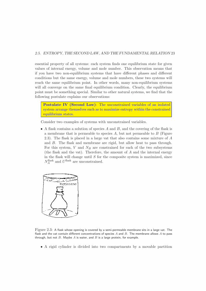
• A flask contains a solution of species A and B, and the covering of the flask isa membrane that is permeable to species A, but not permeable to B (Figure2.3). The flask is placed in a large vat that also contains some mixture of Aand B. The flask and membrane are rigid, but allow heat to pass through.For this system, V and NB are constrained for each of the two subsystems(the flask and the vat). Therefore, the amount of A and the internal energyin the flask will change until S for the composite system is maximized, sinceNflaskA and Uflask are unconstrained.
Figure 2.3: A flask whose opening is covered by a semi-permeable membrane sits in a large vat. Theflask and the vat contain different concentrations of species A and B. The membrane allows A to passthrough, but not B. Maybe A is water, and B is a large protein, for example.
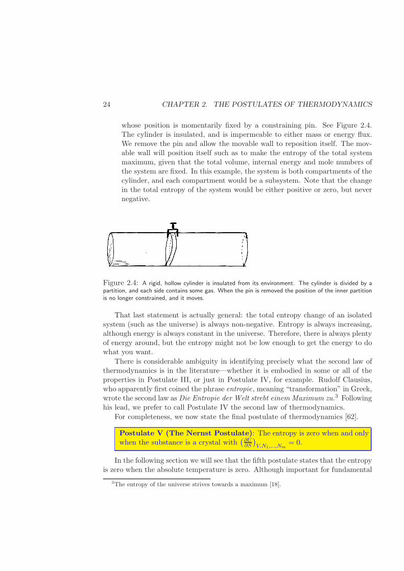
• A rigid cylinder is divided into two compartments by a movable partition
24 CHAPTER 2. THE POSTULATES OF THERMODYNAMICS
whose position is momentarily fixed by a constraining pin. See Figure 2.4.The cylinder is insulated, and is impermeable to either mass or energy flux.We remove the pin and allow the movable wall to reposition itself. The mov-able wall will position itself such as to make the entropy of the total systemmaximum, given that the total volume, internal energy and mole numbers ofthe system are fixed. In this example, the system is both compartments of thecylinder, and each compartment would be a subsystem. Note that the changein the total entropy of the system would be either positive or zero, but nevernegative.
Figure 2.4: A rigid, hollow cylinder is insulated from its environment. The cylinder is divided by apartition, and each side contains some gas. When the pin is removed the position of the inner partitionis no longer constrained, and it moves.
That last statement is actually general: the total entropy change of an isolatedsystem (such as the universe) is always non-negative. Entropy is always increasing,although energy is always constant in the universe. Therefore, there is always plentyof energy around, but the entropy might not be low enough to get the energy to dowhat you want.
There is considerable ambiguity in identifying precisely what the second law ofthermodynamics is in the literature—whether it is embodied in some or all of theproperties in Postulate III, or just in Postulate IV, for example. Rudolf Clausius,who apparently first coined the phrase entropie, meaning “transformation” in Greek,wrote the second law as Die Entropie der Welt strebt einem Maximum zu.3 Followinghis lead, we prefer to call Postulate IV the second law of thermodynamics.
For completeness, we now state the final postulate of thermodynamics [62].
Postulate V (The Nernst Postulate): The entropy is zero when and onlywhen the substance is a crystal with
(∂U∂S
)
V,N1,...,Nm= 0.
In the following section we will see that the fifth postulate states that the entropyis zero when the absolute temperature is zero. Although important for fundamental
3The entropy of the universe strives towards a maximum [18].
2.5. ENTROPY, THE SECONDLAW, AND THE FUNDAMENTAL RELATION 25
questions, or in statistical mechanics, we will not much use the fifth postulate in thisbook. In fact, despite the postulate’s importance, we will often use fundamentalrelations that violate the Nernst Law. Why? Because a fundamental relation isusually only valid over some range of thermodynamic conditions. So, if we use afundamental relation for, say nitrogen, in the regions where it is liquid, gas, or super-critical, but never where it is crystalline, it need not satisfy the Nernst postulate.
An aside about entropy and statistical mechanics.
Entropy always seems strange at first sight—it usually involves symbolssuch as ‘<’ or ‘>’ rather than ‘=’, and it is not conserved. Also, the termstatistical mechanics sounds rather intimidating. However, the ideas instatistical mechanics are rather straightforward, if their implementationis often difficult. Although a quantitative understanding of statisticalmechanics is not necessary to use most of this book, it is sometimes stillenlightening to be aware of its ideas. A fundamental idea of statisticalmechanics—so important that it is on the gravestone of Ludwig vonBoltzmann, is the definition of entropy. That is correct—in statisticalmechanics, entropy is not a fundamental quantity, but is actually defined .There is no definition for energy, so entropy is actually less abstract thanenergy! Boltzmann’s definition for entropy is stunningly simple4
S(U, V,N) := kB log Ω(U, V,N). (2.20)
The first term is called, appropriately enough, the Boltzmann con-stant, and is equal to the ideal gas constant divided by Avogadro’snumber, kB = R/NA. The next term Ω is just a number. It is thenumber of ways that the molecules in a system can arrange themselvesstill keeping the energy fixed at U , the volume fixed at V , and the molenumbers at N .
Imagine a solid crystal of atoms regularly arrayed on a lattice. The posi-tions of the atoms are more-or-less fixed. If we swap the atoms about, westill have the same microscopic state. So, the only possible microscopicarrangements arise from how the energy is distributed. Each atom canvibrate in its position. Or, several atoms can vibrate together. Thegreater the vibration, the more energy an atom has. Maybe one atomis vibrating with all the energy of the crystal, or maybe each atom vi-brates the same as all the others. If we could count up all the ways that
4Here and throughout the text ‘log’ refers to the natural logarithm, and ‘log10’, is log in base10.
26 CHAPTER 2. THE POSTULATES OF THERMODYNAMICS
the energy could distribute itself, we could find the entropy. Statisti-cal mechanics deals with calculating such large numbers. Even withouttackling these sorts of problems, though, we can still think qualitativelyabout entropy.
An ideal gas consists of molecules flying about in a container. Themolecules are very dilute, so they rarely see each other. They are in-dependent. The energy is either stored in the kinetic energy of themolecules, or in the vibrations in the inter-atomic bonds, but only anegligible amount in inter-molecular forces. If the molecules are mono-atomic, they have only kinetic energy. The possible arrangements of themolecules, then, is not just how energy is distributed, but where themolecules are in the container. If we keep the energy constant, how canwe lower the entropy? Well, if we decrease the volume, the molecule hasfewer locations allowed. Hence, Ω goes down. Therefore, the entropy ofan ideal gas decreases with decreasing volume, at constant energy.
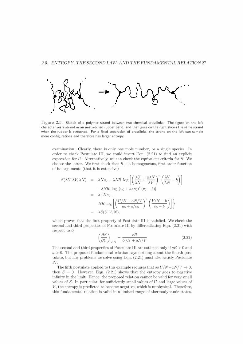
A third example, rubber is made up of cross-linked polymer chains. Be-tween the chemical cross-links, the chain can take many different confor-mations. If we stretch out the rubber, the cross-links become separatedin space. This stretching deformation decreases the number of waysthat the chains can arrange themselves (see Figure 2.5). Hence, stretch-ing rubber decreases its entropy. For a rubber band, the length is moreimportant than the volume, so we substitute L for V in our list of inde-pendent variables. Considering Postulate IV, can you explain why thestretched rubber snaps back when its length is no longer constrained, orwhy a gas under pressure expands?
The reader might find it useful to keep these qualitative ideas in mindwhen trying to understand the thermodynamic behavior of material.
Example 2.5.1 Van der Waals has postulated the following fundamental entropyrelation for a system. Does it satisfy the postulates?
S = Ns0 +NR log
[(U/N + aN/V
u0 + a/v0
)c(V/N − b
v0 − b
)]
,
simple van der Waals fluid. (2.21)
where a, b, c,R, u0, v0 and s0 are constants.
Solution: Internal energy U does play a role. If we also stipulate that Uis conserved, then the first postulate is satisfied. Postulate II is satisfied by
2.5. ENTROPY, THE SECONDLAW, AND THE FUNDAMENTAL RELATION 27
Figure 2.5: Sketch of a polymer strand between two chemical crosslinks. The figure on the leftcharacterizes a strand in an unstretched rubber band, and the figure on the right shows the same strandwhen the rubber is stretched. For a fixed separation of crosslinks, the strand on the left can samplemore configurations and therefore has larger entropy.
examination. Clearly, there is only one mole number, or a single species. Inorder to check Postulate III, we could invert Eqn. (2.21) to find an explicitexpression for U . Alternatively, we can check the equivalent criteria for S. Wechoose the latter. We first check that S is a homogeneous, first-order functionof its arguments (that it is extensive)
S(λU, λV, λN) = λNs0 + λNR log
[(λU
λN+aλN
λV
)c (λV
λN− b
)]
−λNR log [(u0 + a/v0)c(v0 − b)]
= λ Ns0+
NR log
[(U/N + aN/V
u0 + a/v0
)c (V/N − b
v0 − b
)]
= λS(U, V,N),
which proves that the first property of Postulate III is satisfied. We check thesecond and third properties of Postulate III by differentiating Eqn. (2.21) withrespect to U
(∂S
∂U
)
V,N
=cR
U/N + aN/V(2.22)
The second and third properties of Postulate III are satisfied only if cR > 0 anda > 0. The proposed fundamental relation says nothing about the fourth pos-tulate, but any problems we solve using Eqn. (2.21) must also satisfy PostulateIV.
The fifth postulate applied to this example requires that as U/N+aN/V → 0,then S = 0. However, Eqn. (2.21) shows that the entropy goes to negativeinfinity in the limit. Hence, the proposed relation cannot be valid for very smallvalues of S. In particular, for sufficiently small values of U and large values ofV , the entropy is predicted to become negative, which is unphysical. Therefore,this fundamental relation is valid in a limited range of thermodynamic states.
28 CHAPTER 2. THE POSTULATES OF THERMODYNAMICS
However, as long as we stay in the region where entropy is physical, we may usethis equation. In other words, at moderate values for the entropy, our systemmight obey this model. However, as the entropy is lowered, our system can nolonger obey this model, since it violates the Nernst postulate.2
2.6 Definitions of Temperature, Pressure and ChemicalPotential
The postulates have not yet defined the important thermodynamic quantities oftemperature or pressure, which might seem surprising. However, these quantitiesfollow as definitions based on the fundamental quantities introduced in the postu-lates. It is important that these definitions fit our observations about temperatureand pressure. In the following two sections we show that the definitions given inthis section lead to two important intuitive predictions: if two systems with differ-ent temperatures are placed in thermal contact, thermodynamic equilibrium will beattained when the high-temperature body gives enough heat to the low-temperaturebody until they are at the same temperature; two subsystems at different pressuresin mechanical contact reach equilibrium when the high-pressure subsystem expandsat the expense of the low-pressure body until both subsystems are at equal pressures.
We come to the definitions of T and P by considering changes in U . For example,we have already seen in Chapter 1 that work can be done on a system to change itsinternal energy by changing its volume. Similarly, we can change U by adding heator moles. Starting with our fundamental energy relation U(S, V,N1, . . . , Nr), andusing the definition for the differential Eqn. (A.3), we can make the mathematicalobservation
dU =
(∂U
∂S
)
V,NidS +
(∂U
∂V
)
S,NidV +
r∑
i
(∂U
∂Ni
)
S,V,Nj 6=idNi, (2.23)
where, for convenience, we use Ni to mean N1, . . ., Nr, and Nj 6=i means N1, . . .,Ni−1, Ni+1, . . ., Nr. We already know that the (reversible) work done on a systemis −PdV . We also know from experience that volume changes are driven by pres-sure differences between subsystems. Similarly, from experience we know that heattransfers are driven by temperature differences. And finally, the third term on theright side of Eqn. (2.23) suggests that there is some other property that should drivechanges in mole numbers, or mass fluxes. It turns out that these observations canbe predicted by the postulates when we make the following definitions for pressureP , temperature T and chemical potential of species i µi.
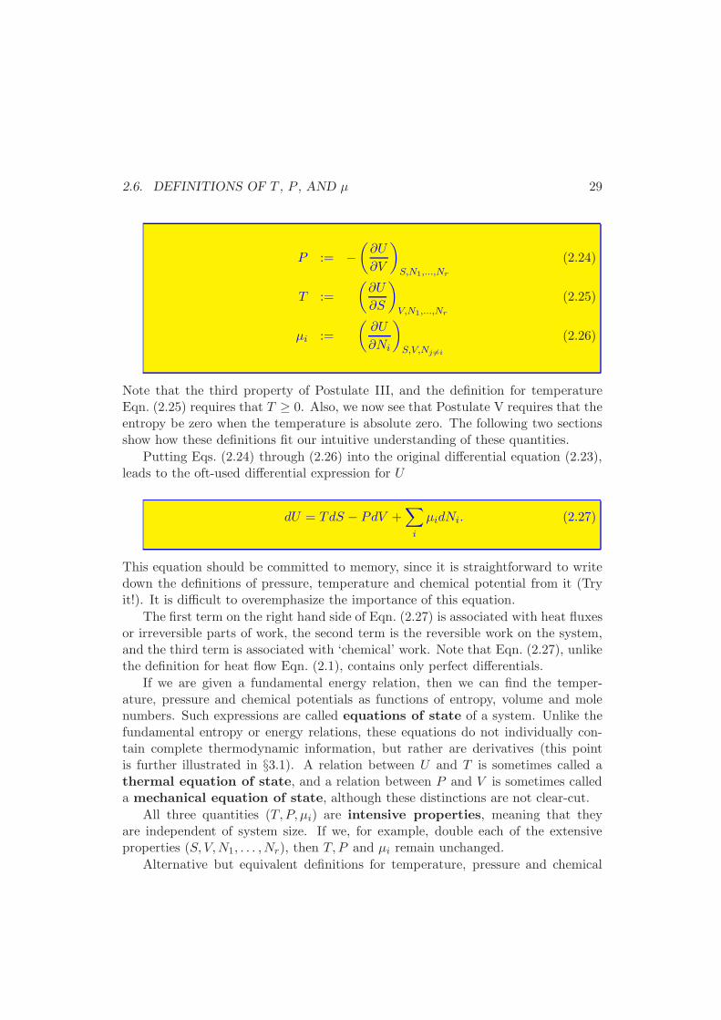
2.6. DEFINITIONS OF T , P , AND µ 29
P := −(∂U
∂V
)
S,N1,...,Nr
(2.24)
T :=
(∂U
∂S
)
V,N1,...,Nr
(2.25)
µi :=
(∂U
∂Ni
)
S,V,Nj 6=i
(2.26)
Note that the third property of Postulate III, and the definition for temperatureEqn. (2.25) requires that T ≥ 0. Also, we now see that Postulate V requires that theentropy be zero when the temperature is absolute zero. The following two sectionsshow how these definitions fit our intuitive understanding of these quantities.
Putting Eqs. (2.24) through (2.26) into the original differential equation (2.23),leads to the oft-used differential expression for U
dU = TdS − PdV +∑
i
µidNi. (2.27)
This equation should be committed to memory, since it is straightforward to writedown the definitions of pressure, temperature and chemical potential from it (Tryit!). It is difficult to overemphasize the importance of this equation.
The first term on the right hand side of Eqn. (2.27) is associated with heat fluxesor irreversible parts of work, the second term is the reversible work on the system,and the third term is associated with ‘chemical’ work. Note that Eqn. (2.27), unlikethe definition for heat flow Eqn. (2.1), contains only perfect differentials.
If we are given a fundamental energy relation, then we can find the temper-ature, pressure and chemical potentials as functions of entropy, volume and molenumbers. Such expressions are called equations of state of a system. Unlike thefundamental entropy or energy relations, these equations do not individually con-tain complete thermodynamic information, but rather are derivatives (this pointis further illustrated in §3.1). A relation between U and T is sometimes called athermal equation of state, and a relation between P and V is sometimes calleda mechanical equation of state, although these distinctions are not clear-cut.
All three quantities (T, P, µi) are intensive properties, meaning that theyare independent of system size. If we, for example, double each of the extensiveproperties (S, V,N1, . . . , Nr), then T, P and µi remain unchanged.
Alternative but equivalent definitions for temperature, pressure and chemical
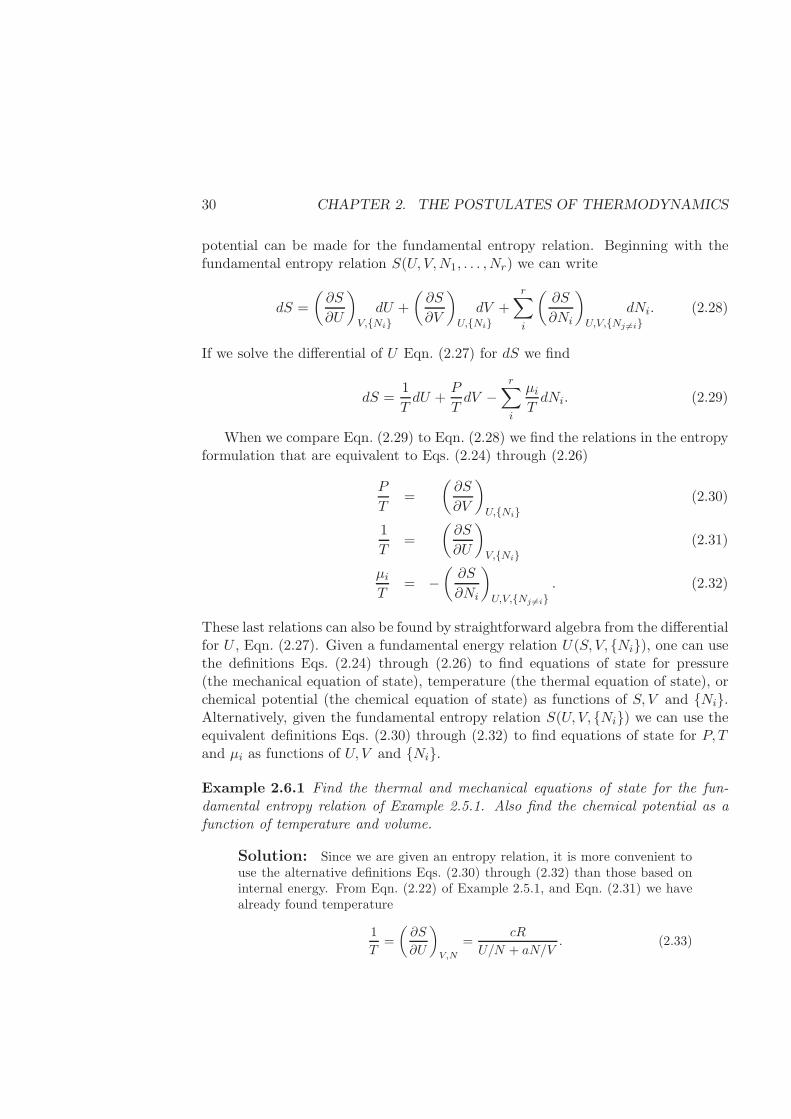
30 CHAPTER 2. THE POSTULATES OF THERMODYNAMICS
potential can be made for the fundamental entropy relation. Beginning with thefundamental entropy relation S(U, V,N1, . . . , Nr) we can write
dS =
(∂S
∂U
)
V,NidU +
(∂S
∂V
)
U,NidV +
r∑
i
(∂S
∂Ni
)
U,V,Nj 6=idNi. (2.28)
If we solve the differential of U Eqn. (2.27) for dS we find
dS =1
TdU +
P
TdV −
r∑
i
µiTdNi. (2.29)
When we compare Eqn. (2.29) to Eqn. (2.28) we find the relations in the entropyformulation that are equivalent to Eqs. (2.24) through (2.26)
P
T=
(∂S
∂V
)
U,Ni(2.30)
1
T=
(∂S
∂U
)
V,Ni(2.31)
µiT
= −(∂S
∂Ni
)
U,V,Nj 6=i. (2.32)
These last relations can also be found by straightforward algebra from the differentialfor U , Eqn. (2.27). Given a fundamental energy relation U(S, V, Ni), one can usethe definitions Eqs. (2.24) through (2.26) to find equations of state for pressure(the mechanical equation of state), temperature (the thermal equation of state), orchemical potential (the chemical equation of state) as functions of S, V and Ni.Alternatively, given the fundamental entropy relation S(U, V, Ni) we can use theequivalent definitions Eqs. (2.30) through (2.32) to find equations of state for P, Tand µi as functions of U, V and Ni.
Example 2.6.1 Find the thermal and mechanical equations of state for the fun-damental entropy relation of Example 2.5.1. Also find the chemical potential as afunction of temperature and volume.
Solution: Since we are given an entropy relation, it is more convenient touse the alternative definitions Eqs. (2.30) through (2.32) than those based oninternal energy. From Eqn. (2.22) of Example 2.5.1, and Eqn. (2.31) we havealready found temperature
1
T=
(∂S
∂U
)
V,N
=cR
U/N + aN/V. (2.33)
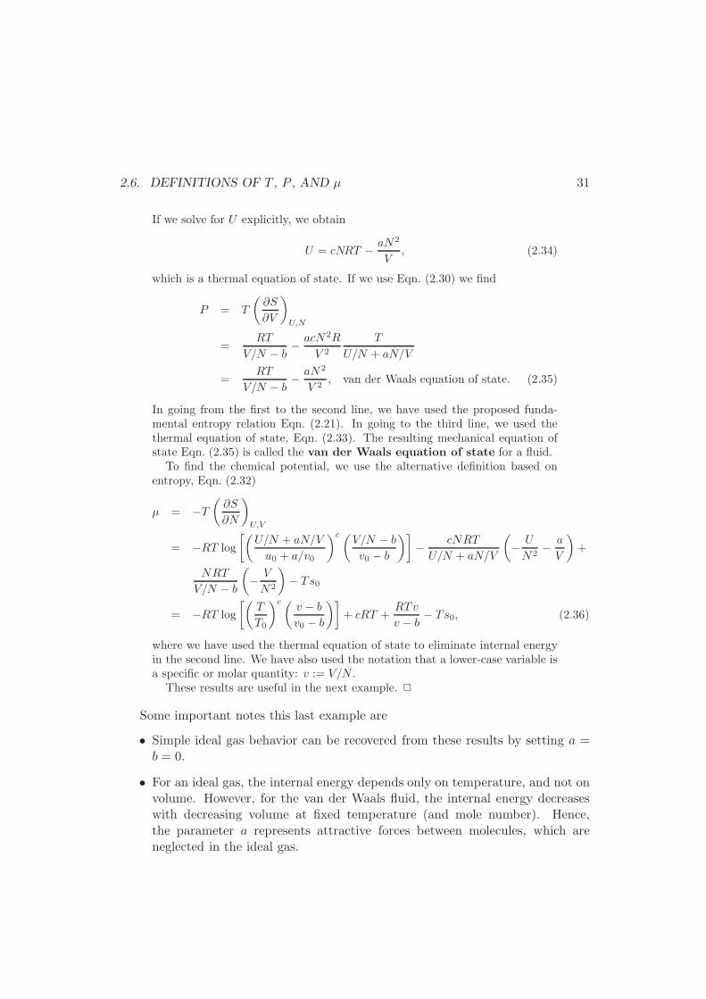
2.6. DEFINITIONS OF T , P , AND µ 31
If we solve for U explicitly, we obtain
U = cNRT − aN2
V, (2.34)
which is a thermal equation of state. If we use Eqn. (2.30) we find
P = T
(∂S
∂V
)
U,N
=RT
V/N − b− acN2R
V 2
T
U/N + aN/V
=RT
V/N − b− aN2
V 2, van der Waals equation of state. (2.35)
In going from the first to the second line, we have used the proposed funda-mental entropy relation Eqn. (2.21). In going to the third line, we used thethermal equation of state, Eqn. (2.33). The resulting mechanical equation ofstate Eqn. (2.35) is called the van der Waals equation of state for a fluid.
To find the chemical potential, we use the alternative definition based onentropy, Eqn. (2.32)
µ = −T(∂S
∂N
)
U,V
= −RT log
[(U/N + aN/V
u0 + a/v0
)c (V/N − b
v0 − b
)]
− cNRT
U/N + aN/V
(
− U
N2− a
V
)
+
NRT
V/N − b
(
− V
N2
)
− Ts0
= −RT log
[(T
T0
)c(v − b
v0 − b
)]
+ cRT +RTv
v − b− Ts0, (2.36)
where we have used the thermal equation of state to eliminate internal energyin the second line. We have also used the notation that a lower-case variable isa specific or molar quantity: v := V/N .
These results are useful in the next example. 2
Some important notes this last example are
• Simple ideal gas behavior can be recovered from these results by setting a =b = 0.
• For an ideal gas, the internal energy depends only on temperature, and not onvolume. However, for the van der Waals fluid, the internal energy decreaseswith decreasing volume at fixed temperature (and mole number). Hence,the parameter a represents attractive forces between molecules, which areneglected in the ideal gas.
32 CHAPTER 2. THE POSTULATES OF THERMODYNAMICS
• The specific volume v is required to be greater than b. Hence, b represents therepulsive forces between molecules that keep the fluid from becoming infinitelydense.
• We cannot simultaneously use the van der Waals mechanical equation of stateand assume that internal energy is independent of volume. The thermal equa-tion of state might have different temperature dependence, but the mechanicaland thermal equations of state come from a single fundamental relation, andmust always be used together.
• We call these equations of state because each one is derived from a fundamentalrelation, but the fundamental relation cannot be derived from a single equationof state. We can say that the fundamental relation has more information thandoes an equation of state.5
Example 2.6.2 If a single-component, simple ideal gas is expanded isentropically
(at constant entropy) until the pressure is halved, what happens to the temperature?
Solution: An ideal gas is one that obeys the mechanical equation of state
PV = NRT, ideal gas equation of state, (2.37)
and the internal energy can be written as a function of temperature only U =U(T ). If the internal energy is also a linear function of temperature, then wecall it a simple ideal gas
U = cNRT, simple ideal gas, thermal equation of state, (2.38)
where c is a constant. We note that the van der Waals fluid of Examples2.5.1 and 2.6.1 reduces to a simple ideal gas when we set a = b = 0. Hence,the fundamental entropy relation for a simple ideal gas can be found fromEqn. (2.21) to be
S = Ns0 +NR log
[(U
Nu0
)cV
Nv0
]
, simple ideal gas. (2.39)
In this problem, we are changing T and P while keeping S constant. Therefore,it is useful to find S = S(T, P ). We can obtain this relation by eliminating Uand V from Eqn. (2.39) using Eqs. (2.37) and (2.38)
S = Ns0 +NR log
[(T
T0
)c+1P0
P
]
, simple ideal gas, (2.40)
5Later we will see (in Chapter 4) that a fundamental relation for a pure species can be derivedfrom two equations of state.
2.6. DEFINITIONS OF T , P , AND µ 33
where T0 := u0/cR and P0 := RT0/v0. From this expression, we see that, inorder to keep the process isentropic, we must keep T c+1/P constant. Hence, ifthe pressure is halved, then the final temperature Tf is
Tf =Ti
21/(c+1), (2.41)
where Ti is the initial temperature. 2
Example 2.6.3 Find the work necessary to complete this process, if it is done quasi-statically. How much heat is transferred?
Solution: If it is done quasi-statically, then the work is
dWqs = −PdV. (2.42)
In order to integrate this equation, we need to determine how the pressure ischanging with the volume. Since the gas is ideal, we can write
P =NRT
V.
However, the temperature is also changing with volume. From Example2.6.2, we determined that an isentropic change in pressure requires that T c+1/Pbe held constant. Hence,
T = Ti
(P
Pi
) 1c+1
.
Inserting this equation into the ideal gas law yields
P =
(NRTiV
) c+1c 1
P1/ci
.
If we insert this expression into our differential equation for quasi-static work,Eqn. (2.42), we obtain
dWqs = −(NRTiV
) c+1c 1
P1/ci
dV.
We may now integrate this equation from the initial volume Vi to the finalvolume; we obtain after some simplification
Wqs = − (NRTi)c+1c
P ci
∫ Vf
Vi
dV
Vc+1c
= cNRTi
[(ViVf
)1/c
− 1
]
. (2.43)
34 CHAPTER 2. THE POSTULATES OF THERMODYNAMICS
But,ViVf
=NRTiPi
Pf
NRTf=
1
2c
c+1.
Hence,
Wqs = cNRTi
[1
21
c+1
− 1
]
. (2.44)
Because Wqs is negative, we find that the gas does work on its surroundingsduring the process. The process might be accomplished by gradually decreasingthe pressure in the environment around the gas allowing it to expand veryslowly. Or, we might remove the weight on a piston very gradually.
We can find the energy transferred during the process from the conservationof energy, or from the definition of Q, Eqn. (2.1)
Qqs = Uf − Ui −Wqs
= cNR (Tf − Ti)− cNRTi
[1
21
c+1
− 1
]
= 0. (2.45)
Therefore, an adiabatic, quasi-static process for an ideal gas is isentropic. Hadthe process been done rapidly, then the required work would have been higher.However, the change in internal energy would be unchanged, so it would havebeen necessary to remove heat from the system in order to keep it isentropic.2
An isentropic process might seem strange at first sight; how can one controlentropy? However, we can prove that the final result of Example 2.6.3 is actu-ally very general: an adiabatic, iso-molar, quasi-static process is isentropic. Fora constant-molar process, the differential for internal energy, Eqn. (2.27), can bewritten
dU = TdS − PdV, closed system (isomolar).
If the process is done quasi-statically, then energy conservation, Eqn. (2.1) allowsus to write this equation
dQqs + dWqs = TdS − PdV, closed system.
Since dWqs = −PdV , we find that
dQqs = TdS, isomolar, (2.46)
which proves that an adiabatic, quasi-static, iso-molar process is isentropic for anymaterial. In fact, some equivalent approaches to thermodynamics treat temperatureas a fundamental quantity and define entropy by this relation. We prefer Callen’sway, because it allows a much easier connection later to statistical mechanics.
2.6. DEFINITIONS OF T , P , AND µ 35
Example 2.6.4 What is the chemical potential of a simple ideal gas as a functionof temperature and pressure?
Solution: We can find the chemical potential from the fundamental relation,Eqn. (2.39), using the alternative definition for µ
µ
T=
(∂S
∂N
)
U,V
= −s0 −R log
[(U
u0N
)cV
v0N
]
− (c+ 1)R
= −s0 −R log
[(T
T0
)cv
v0
]
+ (c+ 1)R. (2.47)
To complete the solution, we multiply each side by T . However, we still need toeliminate v in favor of T and P , which we can do using the ideal gas mechanicalequation of state v = RT/P
µ = −s0T −RT log
[(T
T0
)cRT
Pv0
]
+ (c+ 1)RT
= µ(T ) +RT logP. (2.48)
We have split the result in this way to emphasize the dependence of µ onpressure. Note that the chemical potential of an ideal gas goes to negativeinfinity as the pressure goes to zero. 2
Example 2.6.5 Find the change in temperature for the adiabatic compression ofa simple van der Waals gas. Use this result to find the work required for such acompression.
Solution: If we assume that the process is quasi-static, then the work isrelated to the equilibrium pressure by
dWqs = −PdV. (2.49)
If we use the van der Waals equation of state, Eqn. (2.35), to replace pressure,we see that we cannot integrate this equation, because the temperature is notconstant during the integration. However, we can solve this problem using thethermal equation of state for a simple van der Waals fluid. If we take thedifferential of each side of Eqn. (2.34), we obtain
dU = cNRdT +aN2
V 2dV. (2.50)
When we insert Eqn. (2.50) into Eqn. (2.49) (using dU = dW for an adiabaticprocess), and use the mechanical equation of state, Eqn. (2.35), we obtain
cNRdT = − RT
V/N − bdV, simple van der Waals, adiabatic. (2.51)
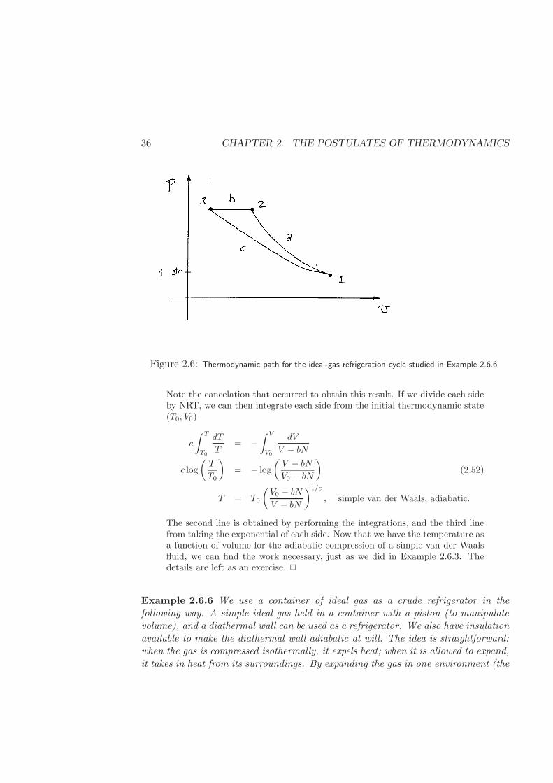
36 CHAPTER 2. THE POSTULATES OF THERMODYNAMICS
Figure 2.6: Thermodynamic path for the ideal-gas refrigeration cycle studied in Example 2.6.6
Note the cancelation that occurred to obtain this result. If we divide each sideby NRT, we can then integrate each side from the initial thermodynamic state(T0, V0)
c
∫ T
T0
dT
T= −
∫ V
V0
dV
V − bN
c log
(T
T0
)
= − log
(V − bN
V0 − bN
)
(2.52)
T = T0
(V0 − bN
V − bN
)1/c
, simple van der Waals, adiabatic.
The second line is obtained by performing the integrations, and the third linefrom taking the exponential of each side. Now that we have the temperature asa function of volume for the adiabatic compression of a simple van der Waalsfluid, we can find the work necessary, just as we did in Example 2.6.3. Thedetails are left as an exercise. 2
Example 2.6.6 We use a container of ideal gas as a crude refrigerator in thefollowing way. A simple ideal gas held in a container with a piston (to manipulatevolume), and a diathermal wall can be used as a refrigerator. We also have insulationavailable to make the diathermal wall adiabatic at will. The idea is straightforward:when the gas is compressed isothermally, it expels heat; when it is allowed to expand,it takes in heat from its surroundings. By expanding the gas in one environment (the
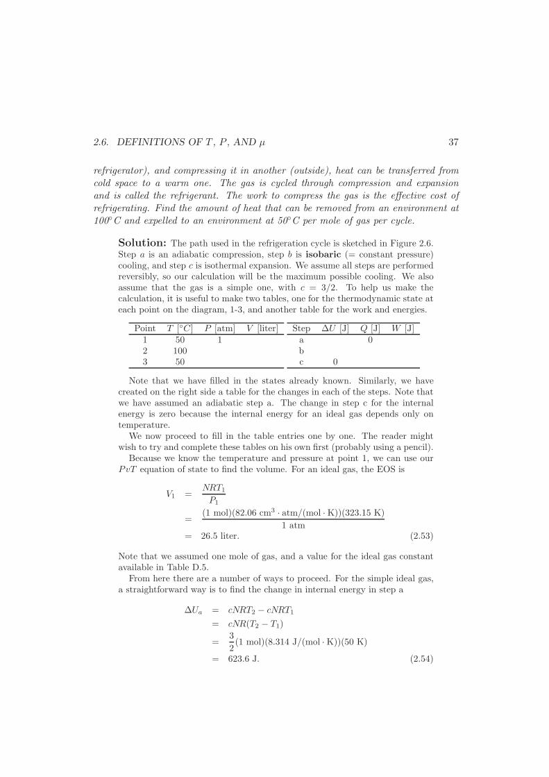
2.6. DEFINITIONS OF T , P , AND µ 37
refrigerator), and compressing it in another (outside), heat can be transferred fromcold space to a warm one. The gas is cycled through compression and expansionand is called the refrigerant. The work to compress the gas is the effective cost ofrefrigerating. Find the amount of heat that can be removed from an environment at100C and expelled to an environment at 50C per mole of gas per cycle.
Solution: The path used in the refrigeration cycle is sketched in Figure 2.6.Step a is an adiabatic compression, step b is isobaric (= constant pressure)cooling, and step c is isothermal expansion. We assume all steps are performedreversibly, so our calculation will be the maximum possible cooling. We alsoassume that the gas is a simple one, with c = 3/2. To help us make thecalculation, it is useful to make two tables, one for the thermodynamic state ateach point on the diagram, 1-3, and another table for the work and energies.
Point T [C] P [atm] V [liter]1 50 12 1003 50
Step ∆U [J] Q [J] W [J]a 0bc 0
Note that we have filled in the states already known. Similarly, we havecreated on the right side a table for the changes in each of the steps. Note thatwe have assumed an adiabatic step a. The change in step c for the internalenergy is zero because the internal energy for an ideal gas depends only ontemperature.
We now proceed to fill in the table entries one by one. The reader mightwish to try and complete these tables on his own first (probably using a pencil).
Because we know the temperature and pressure at point 1, we can use ourPvT equation of state to find the volume. For an ideal gas, the EOS is
V1 =NRT1P1
=(1 mol)(82.06 cm3 · atm/(mol ·K))(323.15 K)
1 atm= 26.5 liter. (2.53)
Note that we assumed one mole of gas, and a value for the ideal gas constantavailable in Table D.5.
From here there are a number of ways to proceed. For the simple ideal gas,a straightforward way is to find the change in internal energy in step a
∆Ua = cNRT2 − cNRT1
= cNR(T2 − T1)
=3
2(1 mol)(8.314 J/(mol ·K))(50 K)
= 623.6 J. (2.54)
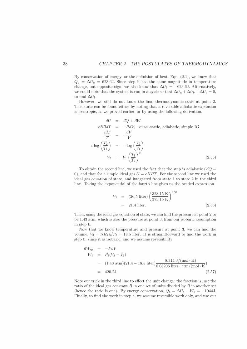
38 CHAPTER 2. THE POSTULATES OF THERMODYNAMICS
By conservation of energy, or the definition of heat, Eqn. (2.1), we know thatQa = ∆Ua = 623.6J. Since step b has the same magnitude in temperaturechange, but opposite sign, we also know that ∆Ub = −623.6J. Alternatively,we could note that the system is run in a cycle so that ∆Ua +∆Ub+∆Uc = 0,to find ∆Ub
However, we still do not know the final thermodynamic state at point 2.This state can be found either by noting that a reversible adiabatic expansionis isentropic, as we proved earlier, or by using the following derivation.
dU = dQ + dW
cNRdT = −PdV, quasi-static, adiabatic, simple IG
cdT
T= −dV
V
c log
(T2T1
)
= − log
(V2V1
)
V2 = V1
(T1T2
)c
(2.55)
To obtain the second line, we used the fact that the step is adiabatic ( dQ =0), and that for a simple ideal gas U = cNRT . For the second line we used theideal gas equation of state, and integrated from state 1 to state 2 in the thirdline. Taking the exponential of the fourth line gives us the needed expression.
V2 = (26.5 liter)
(323.15 K
373.15 K
)3/2
= 21.4 liter. (2.56)
Then, using the ideal gas equation of state, we can find the pressure at point 2 tobe 1.43 atm, which is also the pressure at point 3, from our isobaric assumptionin step b.
Now that we know temperature and pressure at point 3, we can find thevolume, V3 = NRT3/P3 = 18.5 liter. It is straightforward to find the work instep b, since it is isobaric, and we assume reversibility
dWqs = −PdVWb = P2(V2 − V3)
= (1.43 atm)(21.4− 18.5 liter)8.314 J/(mol ·K)
0.08206 liter · atm/(mol ·K)
= 420.2J. (2.57)
Note our trick in the third line to effect the unit change: the fraction is just theratio of the ideal gas constant R in one set of units divided by R in another set(hence the ratio is one). By energy conservation, Qb = ∆Ub −Wb = −1044J.Finally, to find the work in step c, we assume reversible work only, and use our

2.7. TEMPERATURE DIFFERENCES AND HEAT FLOW 39
PvT equation of state
dW = −PdV= −NRT dV
VWc = NRT log(V3/V1)
= (1mol)(8.314J/(mol ·K))(323.15K) log
(18.5liter
26.5liter
)
= −966 J. (2.58)
By energy conservation we know that Qc = −Wc = 966 J. Hence, we have nowcompleted both tables, which look like
Point T [C] P [atm] V [liter]1 50 1 26.52 100 1.43 21.43 50 1.43 18.5
Step ∆U [J] Q [J] W [J]a 623.6 0 623.6b -623.6 -1044 420.2c 0 966 -966
One can define the coefficient of performance as the ratio of the heat ex-tracted divided by the work needed (assuming no work is recovered during theexpansion). Heat is extracted from the environment when Q is positive, whichis in step b. It is necessary to perform work on the gas during steps a andb. Hence, our coefficient of performance is ε = Qc
Wa+Wb= 0.925. Of course,
this assumes complete reversibility. In reality, there are several reasons whythis would not be attained, such as friction in the piston. We also know fromderivations in Appendix C, that any heat flux, such as that necessarily throughthe diathermal wall, will lead to entropy generation, and hence irreversibility.2
2.7 Temperature Differences and Heat Flow
It may seem odd at first to use something abstract like entropy as a fundamentalquantity, and then define an everyday quantity like temperature based on entropy.Therefore, it is important to show that the definition for temperature and the pos-tulates indeed lead to predictions about temperature that fit our experience. Fromexperience, we know that
• Temperature is intensive.
• Two systems in thermal contact reach the same temperature at equilibrium.
• If two objects have different temperatures and are placed in thermal contact,then heat flows from the object of higher temperature to the colder object.
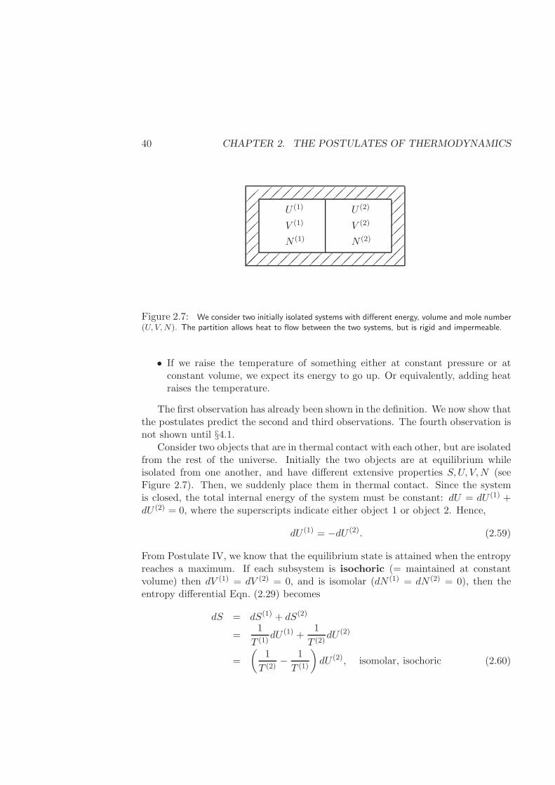
40 CHAPTER 2. THE POSTULATES OF THERMODYNAMICS
U (1) U (2)
V (1) V (2)
N (1) N (2)
Figure 2.7: We consider two initially isolated systems with different energy, volume and mole number(U, V,N). The partition allows heat to flow between the two systems, but is rigid and impermeable.
• If we raise the temperature of something either at constant pressure or atconstant volume, we expect its energy to go up. Or equivalently, adding heatraises the temperature.
The first observation has already been shown in the definition. We now show thatthe postulates predict the second and third observations. The fourth observation isnot shown until §4.1.
Consider two objects that are in thermal contact with each other, but are isolatedfrom the rest of the universe. Initially the two objects are at equilibrium whileisolated from one another, and have different extensive properties S,U, V,N (seeFigure 2.7). Then, we suddenly place them in thermal contact. Since the systemis closed, the total internal energy of the system must be constant: dU = dU (1) +dU (2) = 0, where the superscripts indicate either object 1 or object 2. Hence,
dU (1) = −dU (2). (2.59)
From Postulate IV, we know that the equilibrium state is attained when the entropyreaches a maximum. If each subsystem is isochoric (= maintained at constantvolume) then dV (1) = dV (2) = 0, and is isomolar (dN (1) = dN (2) = 0), then theentropy differential Eqn. (2.29) becomes
dS = dS(1) + dS(2)
=1
T (1)dU (1) +
1
T (2)dU (2)
=
(1
T (2)− 1
T (1)
)
dU (2), isomolar, isochoric (2.60)

2.7. TEMPERATURE DIFFERENCES AND HEAT FLOW 41
where we have used Eqn. (2.59) to obtain the third line. The postulates claim thatthe unconstrained variables—in this case U (2)—will arrange themselves such as tomaximize the entropy. In order to be a maximum, the total entropy must satisfytwo conditions.
First, at equilibrium (∂S/∂U (2))V (1),V (2),N(1),N(2) must be zero. Hence, Eqn. (2.60)
leads to T (2) = T (1) at equilibrium, which is the second observation that we wishedto prove.
Secondly, in order for entropy to be a maximum, entropy must change from alower to a higher value in going from the initial to the final configuration.
(∂S
∂U (2)
)
V (1),V (2),N(1),N(2)
=
(1
T (2)− 1
T (1)
)
. (2.61)
The inequality follows from the postulate that the entropy of an isolated systemmust increase in going from one equilibrium state to another, dS > 0. Eqn. (2.61)
says that if T (2) > T (1), then(
∂S∂U (2)
)
V (1),V (2),N(1),N(2)< 0, then dU (2) < 0 and
heat flows from object 2 to object 1. On the other hand, if T (2) < T (1), then(∂S∂U (2)
)
V (1),V (2),N(1),N(2)> 0, and heat flows from object 1 to object 2. This result
is shown graphically in Figure 2.8. The equilibrium state is the maximum of thecurve. If the initial state lies to the left of the maximum, then U (2) will increase.From Eqn. (2.61), we see that this is when T (1) > T (2). This prediction agrees withour third observation about the intuitive properties of temperature: heat flows fromhot to cold objects.
Example 2.7.1 Two tanks containing a gas insulated and isolated from the envi-ronment are connected by a pipe with a valve. The valve is initially shut, so thetwo tanks are not equilibrated with one another. Tank 1 has volume V1 = 5l, initialpressure P1 = 3atm, and initial temperature T1 = 250K. The second tank has volumeV2 = 2l, initial pressure P2 = 5atm, and initial temperature T2 = 323K. Assumingthat the gas is a simple ideal gas with c = 3/2, find the final temperature of thetanks.
Solution: The walls of the tanks are rigid, so the volume of each tank remainsfixed. The valve allows the gas to pass between the tanks, so the number ofmoles in each tank is not conserved. However, the total number of molesN = N1 + N2 is fixed. The valve also allows energy to pass between the twotanks, so the energy of each tank changes, but the total energy U = U1 + U2
is fixed. Constants of the process are then V1, V2, N , and U . Everything else(N1, N2, T1, T2, S1, S2, P1, P2) can change in reaching the final state.
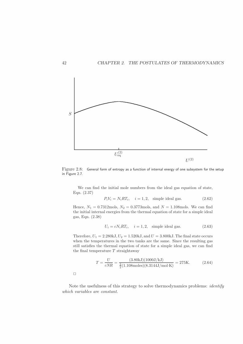
42 CHAPTER 2. THE POSTULATES OF THERMODYNAMICS
U(2)eq
S
U (2)
Figure 2.8: General form of entropy as a function of internal energy of one subsystem for the setupin Figure 2.7.
We can find the initial mole numbers from the ideal gas equation of state,Eqn. (2.37)
PiVi = NiRTi, i = 1, 2, simple ideal gas. (2.62)
Hence, N1 = 0.7312mols, N2 = 0.3773mols, and N = 1.108mols. We can findthe initial internal energies from the thermal equation of state for a simple idealgas, Eqn. (2.38)
Ui = cNiRTi, i = 1, 2, simple ideal gas. (2.63)
Therefore, U1 = 2.280kJ,U2 = 1.520kJ, and U = 3.800kJ. The final state occurswhen the temperatures in the two tanks are the same. Since the resulting gasstill satisfies the thermal equation of state for a simple ideal gas, we can findthe final temperature T straightaway
T =U
cNR=
(3.80kJ)(1000J/kJ)32 (1.108moles)(8.3144J/mol·K) = 275K. (2.64)
2
Note the usefulness of this strategy to solve thermodynamics problems: identifywhich variables are constant.
2.8. PRESSURE DIFFERENCES AND VOLUME CHANGES 43
2.8 Pressure Differences and Volume Changes
In §2.7 we found that our intuition about temperature is predicted by the postulates:temperature differences lead to heat flow from hot to cold objects. Similarly, weshow here that pressure differences lead to changes in volume. In other words, iftwo objects are in mechanical contact, the one at higher pressure will expand at theexpense of the volume of the other object, until the pressures are equal.
Consider two containers of gas that have different temperatures, and differentpressures. Also, we relax the constraint on volume, and allow the volumes of thetwo subsystems to change. (See Figure 2.4.) The two containers are separated by amovable, diathermal partition. Initially, the partition is insulating, and fixed. Then,we allow the partition to move and transfer heat between the two compartments.Throughout the process, the composite system is closed to the universe.
Since the system is closed, again the internal energy is conserved, and Eqn. (2.59)holds. Since the composite system is closed to the universe, the total volume mustalso be conserved, and
dV (1) = −dV (2). (2.65)
Again we hold the mole numbers in each subsystem constant, so that the differ-ential for S Eqn. (2.29) becomes
dS = dS(1) + dS(2)
=1
T (1)dU (1) +
P (1)
T (1)dV (1) +
1
T (2)dU (2) +
P (2)
T (2)dV (2)
=
(1
T (1)− 1
T (2)
)
dU (1) +
(
P (1)
T (1)− P (2)
T (2)
)
dV (1), (2.66)
where we have used Eqs. (2.59) and (2.65) to obtain the third line. Since thevariables U (1) and V (1) are unconstrained, each of the terms on the right side ofthe last line of Eqn. (2.66) must be zero at equilibrium. Hence, we again find thatT (1) = T (2). However, we also find that P (1) = P (2) at equilibrium. Consider thespecial case when the two compartments are at equal temperature T . Then, thechange in volume for the compartments is given by the stipulations that ∆S > 0,according to the postulates. Thus,
T
(∂S
∂V (1)
)
U,V,N(1),N(2)
= P (1) − P (2). (2.67)
If P (1) > P (2), then the volume of V (1) must increase to satisfy the postulates.Likewise P (1) < P (2) requires that V (1) decreases. These results agree with ourobservation about pressure.
44 CHAPTER 2. THE POSTULATES OF THERMODYNAMICS
Example 2.8.1 Find the final pressure of the gas in Example 2.7.1.
Solution:We have now proven that the final state occurs when the temperatures and
pressures in the two tanks are the same. Since the resulting gas still satisfiesthe mechanical equation of state for a simple ideal gas, we can find the finalpressure P
P =NRT
V1 + V2=
(1.108 mols)(0.08206 l·atm/mol·K)(275 K)
7 l= 3.572 atm.
(2.68)2
In Problem 2.8.A, one finds that there is a role played by chemical potentialfor moles analogous to that played by temperature for energy, and by pressure forvolume. Hence, we find that for two systems in thermal, mechanical, and chemicalcontact, equilibrium implies
T (1) = T (2), thermal equilibrium (2.69)
P (1) = P (2), mechanical equilibrium (2.70)
µ(1)1 = µ
(2)1 , chemical equilibrium. (2.71)
These results are completely general6, and should be remembered.
We also find that if the chemical potential of a species is nonuniform, that specieswill move from the region of high chemical potential to the region of low chemicalpotential. Roughly speaking, the chemical potential depends strongly on concentra-tion, so we sometimes say that moles diffuse to offset differences in concentration.However, as stability analysis shows in Chapter 4, that approximation is not alwayscorrect.
2.9 Thermodynamics in One Dimension
So far we have considered systems where the independent variables are (S, V,N),or their conjugates (T, P, µ). However, some important systems are only two di-mensional, such as adsorption on a surface, or a thin film, and, hence, volume plays
6These are completely general for a 3D system in the thermodynamic limit, that is. For 2Dsystems, there may also exist an analog to equal pressure, which is covered in greater detail inChapter 12. Small systems are more subtle [43].
2.9. THERMODYNAMICS IN ONE DIMENSION 45
no role. It is also possible to apply thermodynamics to such systems with a slightmodification to the development we have seen so far. In this section, we considera one-dimensional system—the length of a rubber band. In later sections, we willalso consider two-dimensional systems, such as a catalytic surface and a thin film.
To consider the rubber band, we must use an appropriate replacement for vol-ume, and then the quantity analogous to pressure. For the rubber band, we replacevolume with the length of the rubber band: V → L, and pressure with tension:P → −T . The sign is different, because the work done on a rubber band is +T dL,as opposed to −PdV for a fluid. Hence, we can write the thermodynamic definitionfor tension that is consistent with the mechanical work as
T :=
(∂U
∂L
)
S
. (2.72)
Rubber is comprised of cross-linked polymeric chains; an ideal rubber is made upof one large molecule, so that N = 1/NA, where NA
∼= 6.023× 10²³ is Avogadro’snumber. Therefore, one cannot easily change the size of the system, and thenumber of moles is fixed. Hence, a fundamental entropy relation for a rubber bandmust be of the form S = S(U,L), and extensivity is a little different.
A few simple experiments one can easily perform at home show two importanttrends: (1) the tension in a rubber band increases with length, and (2) the tensionincreases with increasing temperature.7 Hence, any reasonable fundamental relationshould predict these two observations. The latter observation is curious, since itis the opposite of that seen for metal springs, where the tension decreases withtemperature.
In the following example we consider a fundamental entropy relation that wasderived elsewhere from straightforward statistical mechanical arguments.
Example 2.9.1 Treloar [99] has suggested the fundamental entropy relation for arubber band as
S = s0L0 −AcL0R
[
1
2
(L
L0
)2
+
(L0
L
)]
+ cLL0 log
[
1 +U − u0L0
cLL0T0
]
, (2.73)
where s0 and u0 are the specific entropy and internal energy at our reference state,but these are per rubber-band rest length, not per mole. Our reference state is the
7Try suspending a weight with a rubber band, and heating it with a hair dryer. However, becareful to make sure that the rubber band is well equilibrated. Stretch and heat the rubber banda bit first. Then, keeping the weight attached, let the rubber band cool to room temperature.Mark the height of the weight, and then begin warming the rubber band with the dryer. As thetemperature increases, the tension should increase, raising the height of the weight.
46 CHAPTER 2. THE POSTULATES OF THERMODYNAMICS
reference temperature T0 and rest length L0. We have two more constants Ac andcL. The former has something to do with the modulus or rigidity of the rubber band,and the latter is something called the specific constant-length heat capacity. Whatdoes this model predict for tension as a function of length and temperature? Does itagree with experiment?
Solution: To find tension and temperature, we derive two equations of statefrom the fundamental relation. We can find temperature in the usual way fromits (alternative) definition
T := 1
/(∂S
∂U
)
L,Nc
= T0
[
1 +U − U0
CLT0
]
, (2.74)
where we used the fundamental relation Eqn. (2.73) to obtain the second line.From this result we can find the thermal equation of state
U = U0 + CL(T − T0). (2.75)
Curiously, we find that the internal energy does not depend upon length atconstant temperature.
To find the tension in the rubber band, we could use the thermodynamicdefinition Eqn. (2.72). However, it is more convenient to use the alternativeexpression
T = −T(∂S
∂L
)
U,Nc
= ncA0RT
[(L
L0
)
−(L0
L
)2]
(2.76)
where we have again used the fundamental relation Eqn. (2.73). We find severalimportant features of the model from this result:
• The length dependence of the tension given by Eqn. (2.76) has a reason-able shape, but is not exactly what is found from experiment.
• Our thermal equation of state shows that lengthening the rubber band atconstant temperature does not change the internal energy.
• The tension increases linearly with temperature, again in accord withexperiment.8
8We get to see in §3.7.1 the interesting result that the linear dependence in temperature is tieddirectly to the second note above. There we also show how isothermal stretching affects the entropy,but not the energy of a real rubber band.
2.9. THERMODYNAMICS IN ONE DIMENSION 47
• The tension in the rubber band is zero only when its length is L0, itsnatural rest length.
• The second term in the square brackets of Eqn. (2.76) is related to in-compressibility of the rubber band, and shows that a compressive force isnecessary to decrease the length of the rubber band from its rest length.
2
Hence, an isothermal stretch of the rubber band stores no energy in the rubberband. Nonetheless, the rubber band can do work on its environment by pulling upa weight, say. It does this by increasing its entropy . Actually, there is a stronganalogy with compression of an ideal gas. The student should be able to provethat isothermal compression of an ideal gas does not change its internal energy, butrather decreases its entropy.
The fundamental relation considered in the previous example captures many ofthe key experimental features. However, a real rubber band shows richer behavior:
• The internal energy does not grow linearly with temperature.
• At sufficiently low temperatures, the rubber can crystallize, and show no strongelastic behavior.
• The tension deviates from the expression given because of strand entangle-ments and finite extensibility of the strand. Also, at large extensions, therubber can eventually crystallize, or break at large stretches. The physicalmeaning of the constants is now clear. T0 is a reference temperature. The restlength of the rubber band (the length where the tension is zero) is L0.
9
Given the limitations and successes of this fundamental relation, one can drawmany analogies with an ideal gas which also fails at low temperatures and lowvolumes. In other words, the rubber band behaves like an ideal gas, except thatincreasing the length of the rubber band is like decreasing an ideal gas’s volume.For example, compressing an ideal gas isothermally changes the gas’s entropy, butnot its internal energy.
Therefore, we choose to call Eqn. (2.73) a fundamental entropy relation fora simple, ideal rubber band.10 We have shown that this fundamental relation
9From Eqn. (2.75) we see that CL is the constant-length heat capacity. Heat capacities arerigorously defined in §3.5.
10In the language of mechanics, it is the equation that arises for an incompressible, neo-Hookeansolid in extensional deformation.
48 CHAPTER 2. THE POSTULATES OF THERMODYNAMICS
yields
T = Tψ(L)(∂U
∂L
)
T
= 0
(∂S
∂L
)
T
< 0. (2.77)
In words, the last two relations say that isothermal stretching of the rubber banddecreases the entropy, but leaves the internal energy unchanged. In §3.7 we showthat experimental observation of the first relation leads inescapably to the secondand third relations. The results are not too surprising in light of the definition ofentropy on page 25.
2.10 Summary
In this chapter we introduced or used several fundamental quantities:
• Volume V , area A, or length L.
• Mole number N (or numbers, Ni).
• Internal energy U .
• Entropy S.
• Equilibrium states.
The properties of U,S and equilibrium states are described in the four fundamentalpostulates that form the basis of all thermodynamics. We know that a function ofthe form U = U(S, V,N) or one of the form S = S(U, V,N) completely determinesthe thermodynamic properties of a substance.
From these fundamental quantities, we derived
• Temperature T :=(∂U∂S
)
V,N.
• Pressure P := −(∂U∂V
)
S,N.
• Chemical potential µ :=(∂U∂N
)
S,V.
• Heat flow Q: dQ := dU − dW .
2.10. SUMMARY 49
The ideas in the first three definitions are neatly summarized in the differentialfor internal energy
dU = TdS − PdV +r∑
i=1
µidNi. (2.27)
We proved that
• In an iso-molar, quasi-static process dQrev = TdS.
• The fundamental postulates say that heat flows from hot to cold objects untilthe temperatures are equal.
• Compressible objects in mechanical contact change volumes until the pressuresare equal, the higher pressure object expanding at the expense of the other.
• Compounds diffuse across permeable boundaries from regions of high chemicalpotential to regions of low chemical potential.
The last three results were written mathematically for two subsystems (1) and(2) in thermal, mechanical and chemical contact
T (1) = T (2), thermal equilibrium (2.69)
P (1) = P (2), mechanical equilibrium (2.70)
µ(1)1 = µ
(2)1 , chemical equilibrium. (2.71)
All of the above results in the summary should be memorized. In fact, mostproblems of engineering thermodynamics can be solved using only these resultsfrom Chapter 2 plus the results in the following chapters.
We also proved that experimental results imply that
• Compressing an ideal gas isothermally decreases its entropy, but leaves itsinternal energy constant.
• Stretching a rubber band isothermally decreases its entropy, but leaves itsinternal energy constant.
For examples, we used fundamental relations for a simple ideal gas, a simplevan der Waals fluid, and an incompressible, neo-Hookean rubber band. We alsoperformed calculations for work and heat flow of expansion (or contraction), andwork required for adiabatic volume (or length) changes. We showed how an ideal gascan be used as a refrigerator, and estimated the minimum amount of work requiredto do so.
50 CHAPTER 2. THE POSTULATES OF THERMODYNAMICS
2.11 Exercises
2.3.A. The same experiments from Example 2.3.1 are repeated for another gas,which exhibits different results. The first experiment reveals that
(
P +a
V 2
)c (
V − b)c+1
= constant.
The second experiment (using the falling weight) reveals that
dP
dt= − mg
c(V − b)
dl
dt,
where a, b, c are constants. Find the equation of state U = U(P, V ).
2.3.B. Two points on the pressure-volume plane of Example 2.3.1 are connected by aline: PV = constant. Find the work and heat flow necessary to change the volumeand pressure of the container in this example to follow this line from [P0, V0] to[Pf , Vf ]. Find the heat and work necessary to make the system follow a straight linebetween the points. How do your answers compare?
2.3.C. A gas is placed in a container identical to the one in Example 2.3.1. It isreported that the equation of state for the gas is given by
U(P, V ) = U0 +A(PV 2 − P0V
20
).
If the volume is changed slowly (quasi-statically) and adiabatically, how will thepressure change?
2.3.D. The gas in Example 2.3.1 begins at a pressure of 1 atm, and a volume of 1liter. If it is compressed adiabatically to half its original volume, how much work isdone? If a rifle bullet of mass 4g has the same kinetic energy, how fast is it movingin miles/hour? How high must a golf ball (of mass 42g) be raised to gain the sameamount of potential energy?
2.3.E. How much work does it take to compress N = 3 mols of an ideal gas adia-batically from V = 1 liter at T = 24C to a volume of 10ml? The pressure of anideal gas can be found from the temperature and volume by the ideal-gas equationof state PV = NRT .
2.3.F. The gas from Example 2.3.1 is now to be used as part of a refrigeration cycle.To move the fluid in the cycle (look at the tubes in the back of your refrigeratorto see how this fluid is carried), a pump raises its pressure from approximately20 psig at 25C to 32 psig. Assuming that this pump operates adiabatically, andthat the gas is pumped at 23 ft3/min (based on the upstream volume), estimate
2.11. EXERCISES 51
the minimum power (work/time) necessary to pump the fluid. Note that a flowingsystem necessarily has irreversibilities that make the necessary power greater thanyou would predict from a quasi-static process.
2.3.G. We repeat the experiments of Example 2.3.1 with a different gas, and observedifferent behavior. The second experiment reveals that the pressure changes withtime according to
dP
dt= −f0(V )m|~g|dl
dt,
where f0(V ) is some measured function of volume with dimensions of inverse volume.The first experiment reveals
[P − P1(V )]exp
[
−∫ VV0f0(V
′)dV ′]
cf0(V )∼ constant,
where c is a constant, and P1(V ) is another measured function of volume, withdimensions of pressure. V0 is some constant reference volume. Find the equation ofstate U = U(P, V ). Note that Problem 2.3.A is a special case, which might providea check for your answer.
2.4.A A substance called a glassy polymer is placed into a container that allows usto control the work done on and the heat added to the polymer. In State #1, thepolymer has a certain energy U , volume V and mole number N . We measure thepressure at these conditions to be P1, which appears to be stationary with time.
Then, we perform various steps of work on the system, and heat additions andextractions such that the volume and energy are the same as before. We againmeasure the pressure, and find P2 6= P1, but P2 also appears to be stationary.
Are states 1 and 2 at equilibrium? Explain.
2.5.A. Determine which of the following proposed fundamental relations satisfy thepostulates of thermodynamics.
1.
S = s0N +AU1/4V 1/2N1/4
2.
S =
r∑
i=1
Nisi,0 +
(r∑
i=1
Nici
)
log
(U
Nu0
)
+
r∑
i=1
NiR log
(V
v0Ni
)
3.
S = AUNβ
(V 2B
N2
)1/3
52 CHAPTER 2. THE POSTULATES OF THERMODYNAMICS
4.
U =AS3
NV+B
5.
U =AV 3
NS
6.
U =AN2
Vexp (S/NR)
7.
S = Ns0 +NR log[UAV BNC
],
where A,B,C,R, ci, s0, si,0, u0, and v0 are constants.
2.5.B. A simple van der Waals fluid is compressed isentropically to half its volume,if the initial state is (T0, v0), find the final temperature, the work required, and heatflow.
2.5.C. One mole of oxygen at 25C and 15 atm is compressed iso-energetically (=at constant energy) to 35 atm. Calculate the change in entropy using both a simpleideal gas (c = 5/2) and a simple van der Waals fluid. The other parameters for thevan der Waals fluid can be found from the critical properties of oxygen, as shownin §B.3. Compare the two answers. Why are they different? How does your answerfit with the definition of entropy, Eqn. (2.20)?
2.5.D. Do Problem 2.5.C above, but this time use the simplified Redlich-Kwongmodel, Eqn. (2.78) instead of the van der Waals model. You can estimate the
parameter by using the expression A ∼= −6.83RT3/2c .
2.6.A. Find U(P, V,N) for the van der Waals fluid whose fundamental entropy rela-tion is given by Eqn. (2.21). Compare your answer with the result from Problem2.3.A.
2.6.B. Check the postulates, and find P (T, V ) for the following fundamental entropyrelation
S = NR log
(v − b
v0
)
+4b2u3N
3[
3a log(
vv+b
)
− 4Ab]2 , (2.78)
whereR, b, v0 and a are constants. The resulting relation is called the Redlich-Kwongequation of state. Note that the thermal equation of state resulting from Eqn. (2.78)is not particularly accurate. In Chapter 3, a more realistic thermal equation of stateis derived that is compatible with the Redlich-Kwong mechanical equation of state.
2.11. EXERCISES 53
2.6.C. Check the postulates, and find P (T, V ) for the following fundamental energyrelation
U = Na0ψ(v) −N[
R log(v−bv0
)
− a1ψ(v) − s]2
4a2ψ(v), (2.79)
where a0, v0, R, b, a1, a2 and A are constants, and
ψ(v) := A+1
2√2b
log
[
v + b+√2b
v + b−√2b
]
.
The resulting relation is similar to the Peng-Robinson equation of state. Notethat the thermal equation of state resulting from Eqn. (2.79) is not particularlyaccurate. In Chapter 3, a more realistic thermal equation of state is derived that iscompatible with the Peng-Robinson mechanical equation of state.
2.6.D. Check the postulates, and find P (T, V ) for the following fundamental energyrelation
U = Na0ψ(v)−N [R log (v − b)− a1ψ(v)− S/N ]2
4a2ψ(v), (2.80)
where a0, a1, a2, R, b and A are constants, and
ψ(v) := A+1
γ − βlog
(v + β − b
v + γ − b
)
.
The resulting relation is called Martin’s generalized cubic equation of state. Notethat the thermal equation of state resulting from Eqn. (2.80) is not particularlyaccurate. In Chapter 3, a more realistic thermal equation of state is derived that iscompatible with Martin’s generalized mechanical equation of state.
2.6.E. Check the postulates, and find P (T, V ) for the following fundamental entropyrelation
S = Ns0 +NR
log
[(U + aN2/V
u0 + a/v0
)c(V/N − b
v0
)1
N c
]
+
b(V −Nv0)
(V − bN)v0
[
4 +b(V +Nv0 − 2Nb)
(V − bN)v0
]
, (2.81)
where a, v0, R, b and c are constants. The resulting relation is called the Carnahan-Starling generalization to the van der Waals equation of state. Note that the thermalequation of state resulting from Eqn. (2.81) has a constant heat capacity. In Chapter3, a thermal equation of state is derived that yields a better thermal equation ofstate.
54 CHAPTER 2. THE POSTULATES OF THERMODYNAMICS
2.6.F. Check the postulates, and find P (T, V ) for the following fundamental entropyrelation
S = Ns0 +NR log
(V
Nv0
)
− N2R
V
(
B0 +bN
2V
)
− 2ψ2(U, V,N)3/2
3√
Nψ1(V,N), (2.82)
where A0, B0, C0, B1, R, a, b, c, s0, v0, α, γ are constants, and
ψ1(V,N) :=3NC0
V+ 3c
(1
γ+
N2
2V 2
)
exp
(−γN2
V 2
)
+B1
2,
and
ψ2(U, V,N) := Nu0 − U − N2A0
V+aN3
V 2
(αN3
5V 3− 1
2
)
.
The resulting relation is called the Benedict-Webb-Rubin equation of state, com-monly used for alkanes. Note that the thermal equation of state resulting fromEqn. (2.82) is not very accurate. In Chapter 3, a more realistic thermal equation ofstate is derived that is compatible with the PVT equation of state that arises fromEqn. (2.82).
2.6.G Find the work and heat flow necessary to compress a van der Waals fluidisothermally.
2.6.H One mole of a simple ideal gas (c = 3/2) is placed into a container with anearly frictionless piston to be used as a refrigerator. The cycle of the refrigeratorhas three steps. In step (a), the gas is compressed adiabatically from 50C, 1atmto 150C. In step (b), the gas is cooled isobarically back to 50C. In step (c), thegas is expanded back to its original thermodynamic conditions. During step (c), thegas can be used to extract heat from an object at 50C. Find the work necessary tooperate the refrigerator, and the amount of heat that can ideally be extracted.
2.6.I. Find the equations of state for those fundamental relations inProblem 2.5.A.that satisfy the first four thermodynamic postulates.
2.6.J. If you compress a van der Waals fluid isentropically until its volume is halved,what happens to the temperature? Find the quasi-static work, and show that theprocess is also adiabatic.
2.6.K. From Eqn. (2.35), we see that the van der Waals equation of state offers acorrection to the ideal gas through the constants a and b. These constants may befound from the so-called critical properties of a fluid Pc and Tc using Eqn. (4.22).From its critical properties, find a and b for nitrogen. If you have 1 mole of nitrogenat room temperature and pressure, what does the ideal gas model predict for thevolume? What does the van der Waals fluid predict? What is the percentage

2.11. EXERCISES 55
difference? Now do the same calculations for 5atm of pressure. For the van derWaals fluid, you must solve a cubic equation in volume. You may find the equationsin §A.7 useful.
2.6.L. For toluene, we estimate the parameters of the van der Waals equation ofstate to be a = 2.4876432Pa·m6/mol2 and b = 0.000149797m3/mol. Make a plotof specific volume versus pressure for T = 580K, and the range P < 3.78 × 10⁶Paand 6.223 × 10−04 < v < 0.007m3/mol. Note that the van der Waals equationof state is cubic in volume. Hence, you might find the equations in §A.7 useful.What difficulties arise as the pressure approaches 3.78× 10⁶Pa? (Hint: the range ofvolumes given are the physically acceptable roots to the cubic equation for a vapor,as we discuss in detail in §4.2.2.)
2.6.M. For oxygen, we estimate the parameters of the Peng-Robinson equation ofstate to be a = 0.164995Pa·m6/mol2 and b = 1.98414 × 10⁻⁵m3/mol at T = 120K.If you wish to store 1000 moles of oxygen in a 1 cubic meter container, what willthe pressure be? If you triple the pressure, how many moles will be stored in thesame container? Note that the Peng-Robinson equation of state is cubic in volume.Hence, you might find the equations in §A.7 useful.
2.6.N. From Statistical Mechanics it is known that the ideal-gas law holds only whenthe individual molecules rarely interact with one another—i.e., at low densities.However, we can also see this is true from the equations of state. For example, inthe van der Waals equation of state,
P =RT
v − b− a
v2,
we see that the pressure is well approximated by RT/v only for large values of v.To make this criterion more quantitative, we could say that a
v2should be small
relative to RTv . Suppose that we arbitrarily choose an accuracy of 10% as a ‘good’
approximation by an equation of state, then we could require that av2/RTv < 0.10
for the ideal-gas law to hold.
Make plots of vmin, the minimum value of specific volume allowing ideal gas to bea good assumption, as functions of temperature (50–400K). Use the van der Waals,Redlich-Kwong, and Peng-Robinson equations of state for estimates of non-idealbehavior, and assume that the gas is nitrogen. Two of these equations of state areknown to be more accurate. Which is the outlier (i.e., the bad equation of state)?
Note that the parameters for the equation of state can be estimated using thecritical properties of the fluid, as shown in the appendix.
2.6.O. Launching potatoes with an air gun appears to be a popular pastime in ruralparts of the U.S. From a thermodynamics point of view, one uses the work available
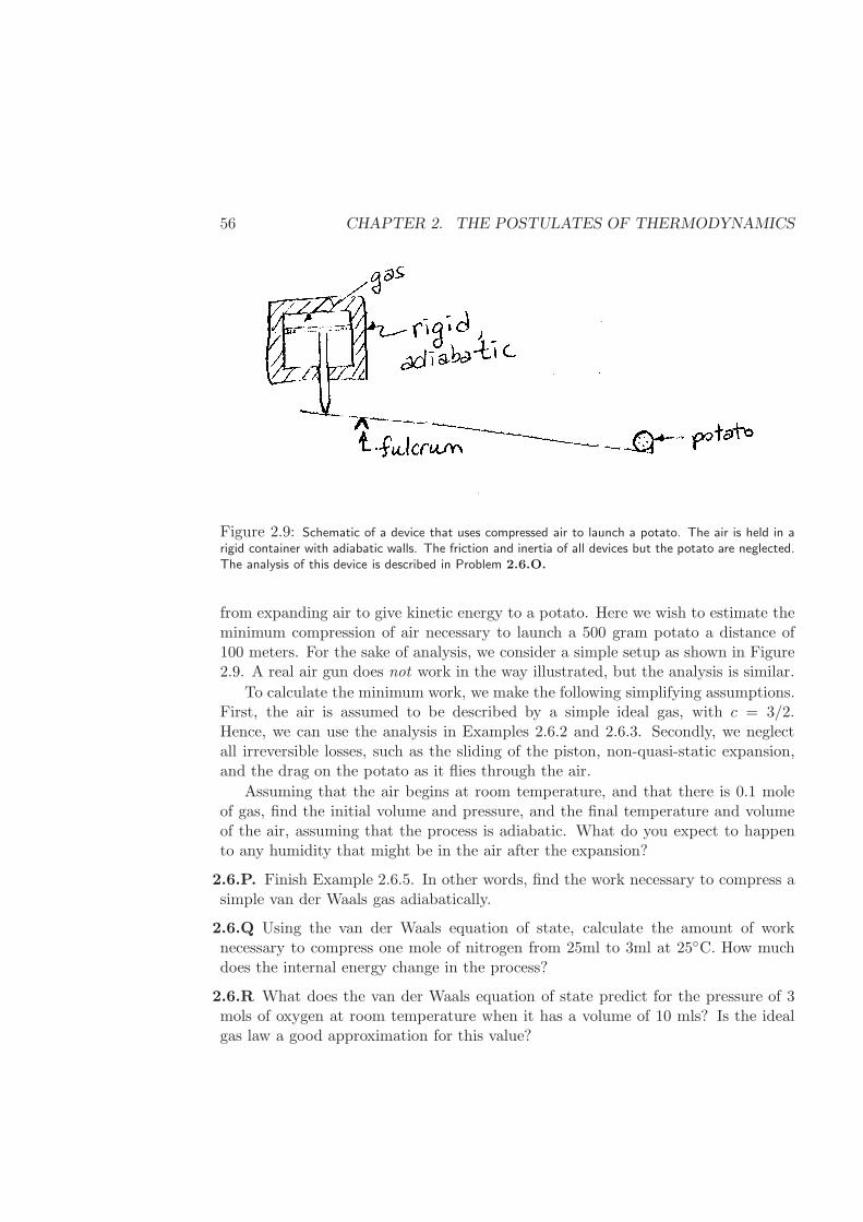
56 CHAPTER 2. THE POSTULATES OF THERMODYNAMICS
Figure 2.9: Schematic of a device that uses compressed air to launch a potato. The air is held in arigid container with adiabatic walls. The friction and inertia of all devices but the potato are neglected.The analysis of this device is described in Problem 2.6.O.
from expanding air to give kinetic energy to a potato. Here we wish to estimate theminimum compression of air necessary to launch a 500 gram potato a distance of100 meters. For the sake of analysis, we consider a simple setup as shown in Figure2.9. A real air gun does not work in the way illustrated, but the analysis is similar.
To calculate the minimum work, we make the following simplifying assumptions.First, the air is assumed to be described by a simple ideal gas, with c = 3/2.Hence, we can use the analysis in Examples 2.6.2 and 2.6.3. Secondly, we neglectall irreversible losses, such as the sliding of the piston, non-quasi-static expansion,and the drag on the potato as it flies through the air.
Assuming that the air begins at room temperature, and that there is 0.1 moleof gas, find the initial volume and pressure, and the final temperature and volumeof the air, assuming that the process is adiabatic. What do you expect to happento any humidity that might be in the air after the expansion?
2.6.P. Finish Example 2.6.5. In other words, find the work necessary to compress asimple van der Waals gas adiabatically.
2.6.Q Using the van der Waals equation of state, calculate the amount of worknecessary to compress one mole of nitrogen from 25ml to 3ml at 25C. How muchdoes the internal energy change in the process?
2.6.R What does the van der Waals equation of state predict for the pressure of 3mols of oxygen at room temperature when it has a volume of 10 mls? Is the idealgas law a good approximation for this value?
2.11. EXERCISES 57
2.6.S Using the Peng-Robinson model from Problem 2.6.C, predict how the pres-sure would change for the adiabatic, reversible compression of the fluid.
2.6.T In Problem 2.3.F you calculate the minimum power to compress an idealgas. Now we consider the adiabatic compression of a gas that is too dense to beideal, and use the van der Waals model to estimate the work. Find the minimumpower to pump hydrogen from 13 atm to 15 atm assuming that the pump operatesadiabatically, and pumped at 23 ft3/min (based on the upstream volume), estimatethe minimum power (work/time) necessary to pump the fluid. For a diatomic gas(like hydrogen) at sufficiently high temperatures, we can assume that the gas issimple, and c = 5/2. The other parameters are found from the expressions in §B.3and the critical properties of the fluid. The critical properties for some fluids arefound in Table D.3 and many more can be found on the NIST Web Book.
You might use the following steps.
• Begin by working in specific quantities only. Find the initial pressure, specificvolume and temperature. From the thermal equation of state, find the specificinternal energy.
• Find the final state of the system assuming reversible, adiabatic compression.Example 2.6.5 might be useful here.
• How is the work (per mole) related to the change in specific internal energy?
• Now find the moles per minute pumped through the system, in order to findthe minimum work per time required of the pump.
2.6.U Estimate the minimum amount of work necessary to use nitrogen as a re-frigerant in the manner shown in Example 2.6.6. However, in this case, the initialpressure is 25 atm, so that we cannot assume that the gas is ideal. Instead use thesimple van der Waals model, with c = 5/2. The other parameters in the model canbe found from the critical properties, as given in §B.3.
2.6.V What is the change in chemical potential predicted by a simple van der Waalsfluid to compress one mole of carbon dioxide isothermally from 15 to 25 bar at 25C?
2.6.W Using the Redlich-Kwong model of Problem 2.6.B, derive an expression topredict the work necessary for an adiabatic, reversible, isomolar compression of afluid.
2.6.X A very realistic PvT equation of state for simple fluids is called the Peng-Robinson model, Eqn. (B.45). Write this equation of state in terms of the com-pressibility factor z := Pv/RT , as a function of v and T . At low densities 1/v, allreal gases behave ideally, and for moderate densities can be described by a virial
58 CHAPTER 2. THE POSTULATES OF THERMODYNAMICS
expansion, Eqn. (B.3). Expand the Peng-Robinson model in a Taylor’s series of 1/varound zero. From this expansion, find expressions for B(T ) and C(T ) predicted bythe Peng-Robinson model.
2.8.A. Consider an isolated system that is separated into two compartments by arigid, diathermal wall that is permeable to species 1, but not to other species inthe system. Show that the postulates indicate that at equilibrium the chemicalpotential of species 1 must be the same in each compartment. Also show that themoles of species 1 move from the compartment of large chemical potential to thecompartment of low chemical potential.
2.8.B. Find the final temperature of the gas in Example 2.7.1 if it is described by asimple van der Waals fluid.
2.8.C. A tank of 1 liter is connected by a pipe fitted with a valve to another tankof 2 liters. Both tanks are insulated and contain Argon, but the first tank is at apressure of 5 bar, and temperature of 220K, whereas the second tank is at a pressureof 10 bar and a temperature of 250K. What are the final temperature and pressurewhen the valve is opened? Assume that the gas is described by a Peng-Robinsonmechanical equation of state, given in §B.6. Also assume that the thermal equationof state is
u = u0 +a0
2√2b
log
[
v + (1 +√2)b
v + (1−√2)b
]
+3
2R (T − T0) .
2.8.D. Assuming that a simple ideal gas with c = 5/2 is used as the refrigerant,design a refrigerator to keep a temperature of 10C with an outside temperatureof 22C. The cycle of the refrigerant has four steps. In the first step, the pistonis used to expand the gas isothermally at the lower temperature. Secondly, thegas is compressed adiabatically until it reaches the higher temperature. Thirdly,it is compressed further at the higher temperature isothermally. Finally, in thefourth step, the gas is expanded adiabatically back to its original thermodynamicconditions. Calculate the amount of work required at each step, and how muchheat is transferred. How much force would you require in your design and howmuch distance to obtain the necessary work? You might find it useful to sketch theprocess on a pressure/volume diagram.
If the refrigerator leaks 1 Joule/hour to the surroundings, how many times perhour must you cycle the refrigerant for your design?
A real refrigerator is only slightly more complicated than this conceptually. First,the refrigerant is cycled by pumping it around a tube, so the process is continuous.Secondly, the refrigerant undergoes phase changes between liquid and gas, which givegreater heat transfers. The details for design of a real system is given in Chapter 5.
2.11. EXERCISES 59
2.8.E. Two tanks are isolated from the environment and connected by a valve. Ini-tially, each tank has oxygen at volumes 10 and 25 liters, and pressures 40atm and27atm, respectively. Each is at temperature 298K. At these pressures, we cannotassume that the gases are ideal. Instead, we use the simple van der Waals fluid(with c = 5/2), and determine the a and b parameters from the critical propertiesof O2 (see §B.3 and Table D.3, or use the NIST Web Book). Determine the finaltemperature and pressure of the tanks after the valve is opened, and equilibrium isreached.
2.9.A. Does the fundamental relation in Example 2.9.1 satisfy the postulates ofthermodynamics?
2.9.B. The following fundamental entropy relation is proposed for a rubber band
S = s0L0 + cLL0 log
[
1 +U − u0L0
cLL0T0
]
+AcL0R
2log
[
1−(L− L0
L1 − L0
)2]
. (2.83)
What does this fundamental relation predict for T (T,L)? What physical interpreta-tion does L1 have? Is this fundamental relation in closer agreement with experiment?
2.9.C. What is the tension as a function of length for a reversible, adiabatic stretchof the rubber band from Example 2.9.1, if the initial length is L0, and the initialtemperature is T0?
2.9.D. A rubber band can also be used as a refrigerator, as in Problem 2.6.H. Byfollowing the cycle drawn in Figure 2.10 in a clockwise fashion, heat can be extractedat the lower temperature from A to B, and expelled at a higher temperature from Cto D. Calculate the amount of work necessary if the refrigerator is operated at hightemperature TH and low temperature TC . Assume that LA = 3L0 and LB = 2L0.Also find the amount of he at extracted during AB and CD for each cycle.
2.9.E. Recent experiments have measured the tension in a single strand of DNA inwater by attaching one end of the strand to a glass slide, and the other end to a 3µmmagnetic bead. By applying a known magnetic field and measuring the extensionof the strand under an optical microscope, a plot of end-to-end length as a functionof tension can be generated [11]. Using straightforward statistical mechanical ideas,fundamental relations can be found for a single DNA molecule. The Gaussian chainmodel in simplified form is
U(S,L,NK) = u0L0 + cLL0T0
exp
[S − s0cL
− kBL2
2cLL0NKa2K
]
− 1
, (2.84)
where u0, T0, and s0 are constants with straightforward interpretation, kB is Boltz-mann’s constant (equal to the ideal gas constant divided by Avogadro’s number),
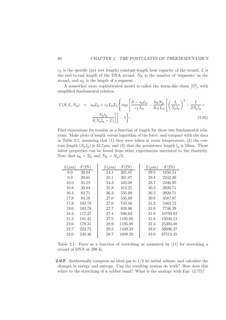
60 CHAPTER 2. THE POSTULATES OF THERMODYNAMICS
cL is the specific (per rest length) constant-length heat capacity of the strand, L isthe end-to-end length of the DNA strand, NK is the number of ‘segments’ in thestrand, and aK is the length of a segment.
A somewhat more sophisticated model is called the worm-like chain [57], withsimplified fundamental relation
U(S,L,Np) = u0L0 + cLL0T0
exp
[
S − s0L0
cLL0− kBNp
2cLL0
[(L
Nplp
)2
− L
2Nplp+
Nplp4(Nplp − L)
]]
− 1
. (2.85)
Find expressions for tension as a function of length for these two fundamental rela-tions. Make plots of length versus logarithm of the force, and compare with the datain Table 2.1, assuming that (1) they were taken at room temperature, (2) the con-tour length (Nplp) is 32.7µm, and (3) that the persistence length lp is 53nm. Theselatter properties can be found from other experiments unrelated to the elasticity.Note that aK = 2lp and NK = Np/2.
L(µm) F (fN)
8.0 30.049.3 29.0110.0 35.1510.8 39.0416.4 82.7117.9 84.1617.8 103.7819.0 103.7818.3 117.2721.2 181.4522.0 178.3122.7 223.7523.0 248.46
L(µm) F (fN)
24.1 301.0725.1 301.0724.3 442.0825.8 412.2526.3 535.6927.0 535.6927.0 733.5027.7 828.8627.4 936.6227.5 1195.9828.9 1195.9829.5 1449.2328.7 1609.29
L(µm) F (fN)
29.5 1850.5429.4 2242.3929.7 2446.9530.3 3920.7130.3 3920.7130.6 4587.8731.2 5463.1231.6 7746.3931.8 10793.8231.6 15040.1232.4 25394.4833.0 56696.2733.0 67512.45
Table 2.1: Force as a function of stretching as measured by [11] for stretching astrand of DNA at 298 K.
2.9.F. Isothermally compress an ideal gas to 1/2 its initial volume, and calculate thechanges in energy and entropy. Can the resulting system do work? How does thisrelate to the stretching of a rubber band? What is the analogy with Eqs. (2.77)?
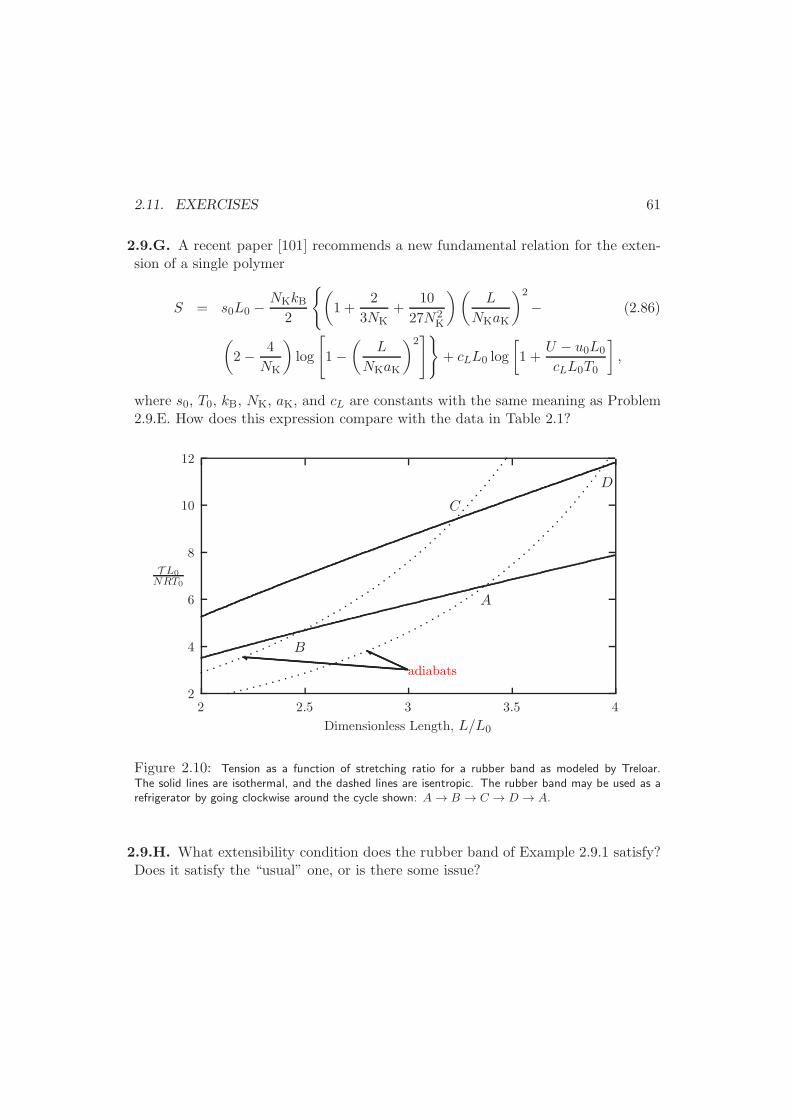
2.11. EXERCISES 61
2.9.G. A recent paper [101] recommends a new fundamental relation for the exten-sion of a single polymer
S = s0L0 −NKkB
2
(
1 +2
3NK+
10
27N2K
)(L
NKaK
)2
− (2.86)
(
2− 4
NK
)
log
[
1−(
L
NKaK
)2]
+ cLL0 log
[
1 +U − u0L0
cLL0T0
]
,
where s0, T0, kB, NK, aK, and cL are constants with the same meaning as Problem2.9.E. How does this expression compare with the data in Table 2.1?
2
4
6
8
10
12
2 2.5 3 3.5 4
T L0NRT0
Dimensionless Length, L/L0
adiabats
A
B
C
D
y Y
Figure 2.10: Tension as a function of stretching ratio for a rubber band as modeled by Treloar.The solid lines are isothermal, and the dashed lines are isentropic. The rubber band may be used as arefrigerator by going clockwise around the cycle shown: A → B → C → D → A.
2.9.H. What extensibility condition does the rubber band of Example 2.9.1 satisfy?Does it satisfy the “usual” one, or is there some issue?

62 CHAPTER 2. THE POSTULATES OF THERMODYNAMICS
Chapter 3
Generalized ThermodynamicPotentials
A theory is the more impressive the greater the simplicityof its premises, the more different kinds of things it relates,and the more extended is its area of applicability. Therefore
the deep impression which classical thermodynamics made upon me.It is the only physical theory of universal content concerning
which I am convinced that, within the framework of the applicabilityof its basic concepts, it will never be overthrown (for the special
attention of those who are skeptics on principle).
– Albert Einstein1
From the postulates in Chapter 2, we have already seen that from U(S, V ,N1, . . ., Nm) or S(U , V , N1, . . ., Nm) we can derive all thermodynamic informa-tion about a system. For example, we can find mechanical or thermal equationsof state. However, we also know that it is sometimes convenient to use other in-dependent variables besides entropy and volume. For example, when we performan experiment at room temperature open to the atmosphere, we are manipulatingtemperature and pressure, not entropy and volume. In this case, the more naturalindependent variables are T and P . Then, the question arises: Is there a functionof (T, P,N1, . . . , Nm) that contains complete thermodynamic information? In otherwords, is there some function, say G(T, P,N1, . . . , Nm) from which we could deriveall the equations of state? It turns out that such functions do exist, and that theyare very useful for solving practical problems.
1 Albert Einstein: Philosopher-Scientist, p.33, ed. by P. A. Schilpp, (Cambridge U.P., London,1970)
63
64 CHAPTER 3. GENERALIZED THERMODYNAMIC POTENTIALS
In the first section we show how to derive such a function for any complete set ofindependent variables using Legendre Transforms. In this book we introduce threewidely used potentials: the enthalpy H(S,P,N1, . . . , Nm), the Helmholtz potentialF (T, V,N1, . . . , Nm), and the Gibbs free energy G(T, P,N1, . . . , Nm). These func-tions that contain complete thermodynamic information using independent variablesbesides S, V and N1, . . . , Nm are called generalized thermodynamic potentials.
These quantities are essential for engineering or applied thermodynamics. Forexample, we already know that an isolated system attains equilibrium when theentropy is maximized. However, a system in contact with a thermal reservoir at-tains equilibrium when the Helmholtz potential F is minimized. We show below(Examples 3.2.1 and 3.2.2), that the work necessary to compress any gas isother-mally is just the change in F (T, V,N). In a fuel cell, G(T, P,N) is important. Or,in the open (flowing) systems considered in Chapter 5, we see that another suchfunction (called enthalpy) is also important. In other words, we need not considerthe entropy of the reservoir explicitly to find equilibrium.
In §3.2, we show how subsystems in contact with thermal and/or mechanicalreservoirs are handled more naturally using the generalized potentials. In §3.6 weshow how to express any derivative in terms of the measurable quantities introducedin §3.5.
In §3.3, we see that the generalized thermodynamic potentials have a relationshipbetween derivatives of the independent variables called the Maxwell relations. Theserelations are essential for the thermodynamic manipulations discussed in the nextchapter, and are used in the remainder of the text.
3.1 Legendre Transforms
Recall Example 2.6.1, where we found U(T, V,N) from S(U, V,N). Although wecould find P (T, V,N) from the S expression, it is not possible to find it fromU(T, V,N). Hence, we lose information when we go from the fundamental rela-tion to the equation of state. In this section we show why that is, and introduce amethod to find a function F (T, V,N) that has all the information that was in ouroriginal fundamental relation S(U, V,N).
The Naıve Approach
On first reflection, we might think that finding a function with complete thermo-dynamic information that has T instead of S as an independent variable is straight-forward. We would naıvely take the derivative of U(S) with respect to S to findT (S), invert, and insert S(T ) into U(S(T )) to find U(T ). However, we can showthat such a naıve approach would lead to a loss of information along the way.
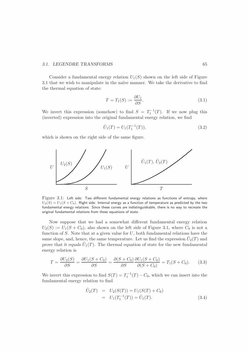
3.1. LEGENDRE TRANSFORMS 65
Consider a fundamental energy relation U1(S) shown on the left side of Figure3.1 that we wish to manipulate in the naıve manner. We take the derivative to findthe thermal equation of state:
T = T1(S) :=∂U1
∂S. (3.1)
We invert this expression (somehow) to find S = T−11 (T ). If we now plug this
(inverted) expression into the original fundamental energy relation, we find
U1(T ) = U1(T−11 (T )), (3.2)
which is shown on the right side of the same figure.
U
S
U1(S)U2(S)
U
T
U1(T ), U2(T )
Figure 3.1: Left side: Two different fundamental energy relations as functions of entropy, whereU2(S) = U1(S +C0). Right side: Internal energy as a function of temperature as predicted by the twofundamental energy relations. Since these curves are indistinguishable, there is no way to recreate theoriginal fundamental relations from these equations of state.
Now suppose that we had a somewhat different fundamental energy relationU2(S) := U1(S + C0), also shown on the left side of Figure 3.1, where C0 is not afunction of S. Note that at a given value for U , both fundamental relations have thesame slope, and, hence, the same temperature. Let us find the expression U2(T ) andprove that it equals U1(T ). The thermal equation of state for the new fundamentalenergy relation is
T =∂U2(S)
∂S=∂U1(S + C0)
∂S=∂(S + C0)
∂S
∂U1(S + C0)
∂(S + C0)= T1(S + C0). (3.3)
We invert this expression to find S(T ) = T−11 (T )−C0, which we can insert into the
fundamental energy relation to find
U2(T ) = U2(S(T )) = U1(S(T ) + C0)
= U1(T−11 (T )) = U1(T ). (3.4)
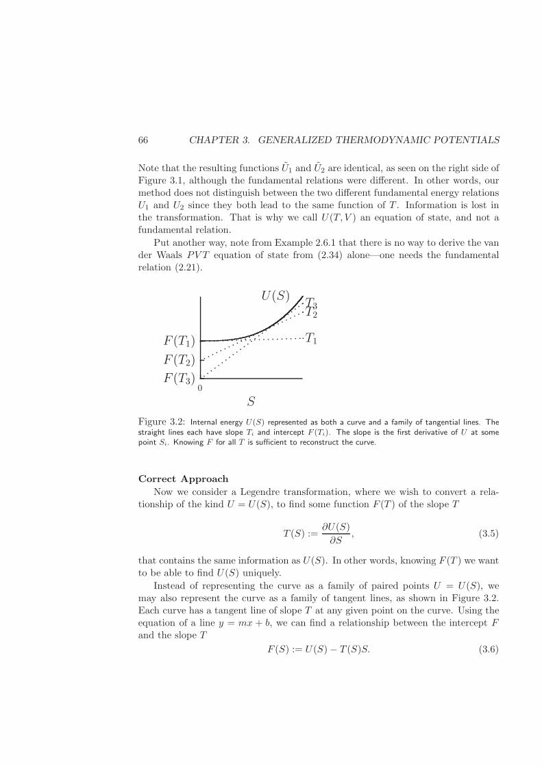
66 CHAPTER 3. GENERALIZED THERMODYNAMIC POTENTIALS
Note that the resulting functions U1 and U2 are identical, as seen on the right side ofFigure 3.1, although the fundamental relations were different. In other words, ourmethod does not distinguish between the two different fundamental energy relationsU1 and U2 since they both lead to the same function of T . Information is lost inthe transformation. That is why we call U(T, V ) an equation of state, and not afundamental relation.
Put another way, note from Example 2.6.1 that there is no way to derive the vander Waals PV T equation of state from (2.34) alone—one needs the fundamentalrelation (2.21).
F (T1)
F (T2)
F (T3)0
S
T1
T2T3
U(S)
Figure 3.2: Internal energy U(S) represented as both a curve and a family of tangential lines. Thestraight lines each have slope Ti and intercept F (Ti). The slope is the first derivative of U at somepoint Si. Knowing F for all T is sufficient to reconstruct the curve.
Correct Approach
Now we consider a Legendre transformation, where we wish to convert a rela-tionship of the kind U = U(S), to find some function F (T ) of the slope T
T (S) :=∂U(S)
∂S, (3.5)
that contains the same information as U(S). In other words, knowing F (T ) we wantto be able to find U(S) uniquely.
Instead of representing the curve as a family of paired points U = U(S), wemay also represent the curve as a family of tangent lines, as shown in Figure 3.2.Each curve has a tangent line of slope T at any given point on the curve. Using theequation of a line y = mx + b, we can find a relationship between the intercept Fand the slope T
F (S) := U(S)− T (S)S. (3.6)
3.1. LEGENDRE TRANSFORMS 67
From Eqs. (3.5) and (3.6), we can eliminate S to find F (T ). To reconstruct U(S)from F (T ), note that
S(T ) = −∂F∂T
, (3.7)
so that we can solve Eqn. (3.6) for U
U(T ) = F (T )− T∂F
∂T. (3.8)
From Eqs. (3.7) and (3.8) we can eliminate T to find U(S). Hence, knowing F (T )allows us to reconstruct the entire curve.
Therefore, we define the Helmholtz potential F to be the Legendre transformof U(S) by Eqn. (3.6). Similarly, if we perform the Legendre transform on U(V ), weobtain the enthalpy H as the Legendre transform; we can perform the Legendretransform simultaneously on both arguments of U(S, V ) to obtain the Gibbs freeenergy G.
H(S,P,N1, . . . , Nm) := U + PV (3.9)
F (T, V,N1, . . . , Nm) := U − TS (3.10)
G(T, P,N1, . . . , Nm) := U − TS + PV (3.11)
Note that the sign is different for the transformation from V to P , because theslope of U(V ) is −P . For each of the three transforms, we can reconstruct theoriginal fundamental energy relation by Eqs. (3.7) and (3.8). The results of theinversion are summarized in Table 3.1. For a given general potential, only one setof independent variables gives complete thermodynamic information. We call themembers of this set the canonical independent variables for that potential.
Example 3.1.1 Find the Helmholtz potential as a function of temperature and vol-ume for a pure-component, simple, ideal gas, which has the fundamental entropyrelation
S = Ns0 +NR log
[(U
u0
)c(V
v0
)(1
N1+c
)]
, (3.12)
where s0 is the specific entropy at reference point (u0, v0, N0).
Solution: From the definition of the Helmholtz potential Eqn. (3.10), wesee that we need both U and S as functions of T and V . Hence, we need thethermal equation of state. Since we have a fundamental entropy formulation,

68 CHAPTER 3. GENERALIZED THERMODYNAMIC POTENTIALS
From Find canonical To find Internal Energy Elim-independent variables U(S, V ) inate
H(S,P ) V (S,P ) =(∂H∂P
)
S,NU(S,P ) = H(S,P )− PV (S,P ) P
F (T, V ) S(T, V ) = −(∂F∂T
)
V,NU(T, V ) = F (T, V ) + TS(T, V ) T
G(T, P ) S(T, P ) = −(∂G∂T
)
P,NU(T, P ) = G(T, P ) + TS(T, P ) T, P
V (T, P ) =(∂G∂P
)
T,N−PV (T, P )
Table 3.1: How to recover the fundamental energy relation U(S, V ) from the generalized thermody-namic potentials F,G and H as functions of their canonical independent variables: Given a fundamentalrelation of the quantity in the first column, use equations in the second and third columns to eliminatethe variables in the fourth column leaving U = U(S, V ).
we use the alternative definition of temperature Eqn. (2.31) to find the thermalequation of state
1
T:=
(∂S
∂U
)
V,N
=cNR
U, (3.13)
which we may use to find U = U(T ). When Eqn. (3.13) is inserted into the fun-damental entropy relation for an ideal gas, Eqn. (3.12) we obtain an expressionfor S(T, V,N)
S = Ns0 +NR log
[(T
T0
)c (V
Nv0
)]
, (3.14)
where T0 := u0/cR. We now have the sought-after expressions for U =U(T, V ) and S = S(T, V ). When we insert the expression we found for U(T ),Eqn. (3.13), and Eqn. (3.14) into the definition for F , Eqn. (3.10), we find
F = Nf0 + (cNR−Ns0)(T − T0)−NRT log
[(T
T0
)c (V
Nv0
)]
, (3.15)
where f0 := u0 − s0T0 is the specific Helmholtz potential at the reference state(T0, v0). Eqn. (3.15) contains all thermodynamic information about a simpleideal gas, as does Eqn. (3.12) 2
3.1. LEGENDRE TRANSFORMS 69
Example 3.1.2 The Helmholtz potential for a system is given as
F = Nf0 −Ns0(T − T0) +N
∫ T
T0
(T ′ − T
T ′
)
cidealv (T ′)dT ′ (3.16)
−NRT log
(V
v0N
)
where s0, T0, f0 and v0 are constants with straightforward interpretation, and cidealv (T )is some known function of temperature. Can you find the fundamental energy rela-tion?
Solution: We use the prescription in Table 3.1. Using the second row(which follows from the differential for F ), we find S(T, V ) from Eqn. (3.16)
S = −(∂F
∂T
)
V,N
(3.17)
= Ns0 +N
∫ T
T0
cidealv (T ′)
T ′dT ′ +NR log
[V
v0N
]
.
We used the Leibniz rule for differentiating an integral Eqn. (A.25) to obtainthe second line. We find an expression for U from the second column of Table3.1
U = F + TS (3.18)
= Nf0 +NsoT0 +N
∫ T
T0
cidealv (T ′)dT ′.
If we could invert Eqn. (3.17) to find T (S, V,N), we could insert this expres-sion into the upper limit of the integral in Eqn. (3.18) to obtain U(S, V,N),and we would be finished. However, practically speaking, the inversion is im-possible without specifying cidealv (T ), and in practice is difficult to do for nearlyall expressions cidealv (T ). This is as close as we can come to finding a funda-mental energy relation, since Eqs. (3.17) and (3.18) are sufficient to determineU(S, V,N). 2
This example shows that it is more natural to use F when T and V are theindependent variables; the single equation (3.16) gives complete thermodynamicinformation, whereas we require both Eqn. (3.17) and (3.18) to express the funda-mental energy relation.
Note that we have internal energy as a function of temperature only U = U(T )in the thermal equation of state, Eqn. (3.18), but independent of volume. We see inExample 3.1.3 below that the mechanical equation of state is simply the ideal gaslaw. Hence, Eqn. (3.16) is the fundamental Helmholtz relation for a general ideal
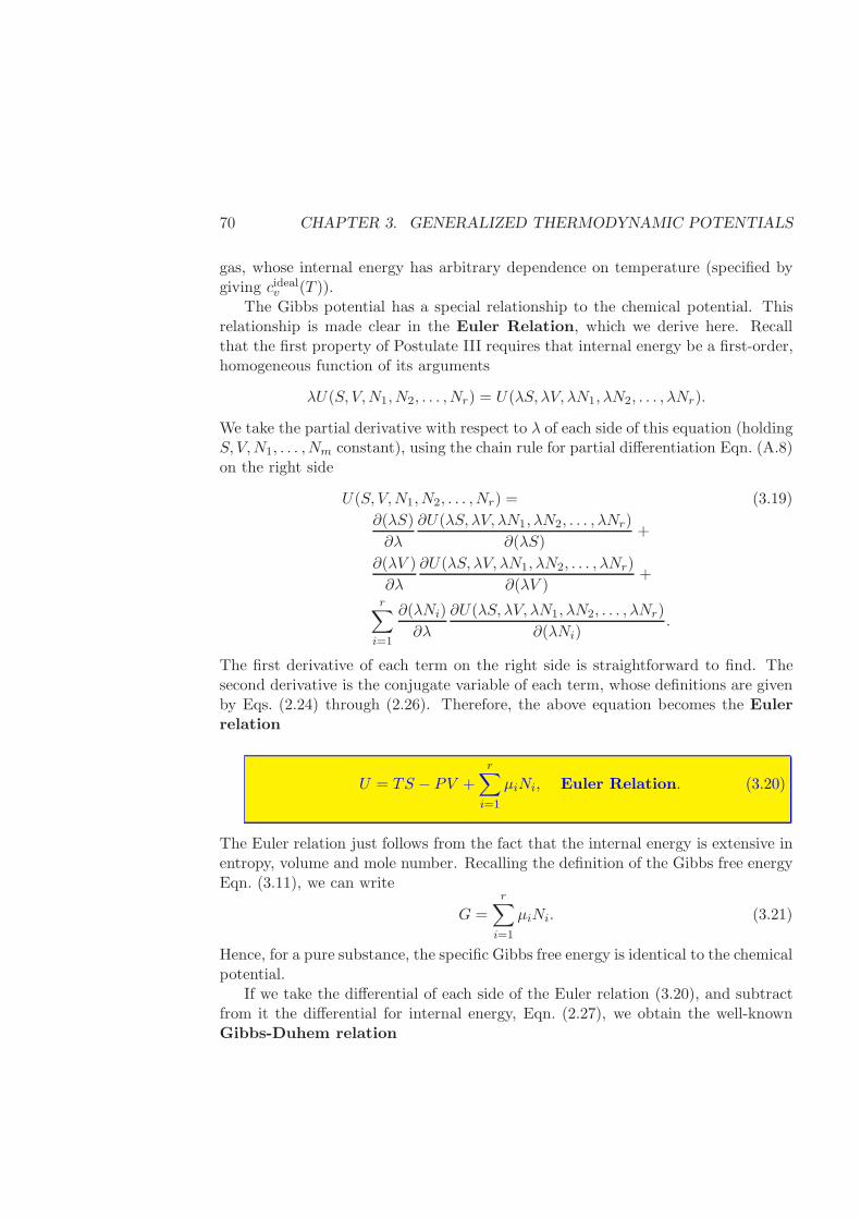
70 CHAPTER 3. GENERALIZED THERMODYNAMIC POTENTIALS
gas, whose internal energy has arbitrary dependence on temperature (specified bygiving cidealv (T )).
The Gibbs potential has a special relationship to the chemical potential. Thisrelationship is made clear in the Euler Relation, which we derive here. Recallthat the first property of Postulate III requires that internal energy be a first-order,homogeneous function of its arguments
λU(S, V,N1, N2, . . . , Nr) = U(λS, λV, λN1, λN2, . . . , λNr).
We take the partial derivative with respect to λ of each side of this equation (holdingS, V,N1, . . . , Nm constant), using the chain rule for partial differentiation Eqn. (A.8)on the right side
U(S, V,N1, N2, . . . , Nr) = (3.19)
∂(λS)
∂λ
∂U(λS, λV, λN1, λN2, . . . , λNr)
∂(λS)+
∂(λV )
∂λ
∂U(λS, λV, λN1, λN2, . . . , λNr)
∂(λV )+
r∑
i=1
∂(λNi)
∂λ
∂U(λS, λV, λN1, λN2, . . . , λNr)
∂(λNi).
The first derivative of each term on the right side is straightforward to find. Thesecond derivative is the conjugate variable of each term, whose definitions are givenby Eqs. (2.24) through (2.26). Therefore, the above equation becomes the Eulerrelation
U = TS − PV +
r∑
i=1
µiNi, Euler Relation. (3.20)
The Euler relation just follows from the fact that the internal energy is extensive inentropy, volume and mole number. Recalling the definition of the Gibbs free energyEqn. (3.11), we can write
G =
r∑
i=1
µiNi. (3.21)
Hence, for a pure substance, the specific Gibbs free energy is identical to the chemicalpotential.
If we take the differential of each side of the Euler relation (3.20), and subtractfrom it the differential for internal energy, Eqn. (2.27), we obtain the well-knownGibbs-Duhem relation
3.2. EXTREMA PRINCIPLES FOR THE POTENTIALS 71
0 = SdT − V dP +
r∑
i=1
Nidµi, Gibbs-Duhem Relation. (3.22)
Finally, we note that one may also take the Legendre Transform of the entropy.Such functions are called Massieu functions [13, §5-4]. Problem 3.3.D considersa transform on N , for example. A systematic way to handle any such transformmay be found in the textbook by Tester, Modell and Reid [59, 98, §§5-4,5].
Example 3.1.3 Prove that the Helmholtz potential given by Eqn. (3.16)
F = Nf0 −Ns0(T − T0) +N
∫ T
T0
(T ′ − T
T ′
)
cidealv (T ′)dT ′
−NRT log
(V
v0N
)
.
leads to the ideal-gas mechanical equation of state
Solution: Using Eqn. (3.52) we can find the mechanical equation of statefrom the Helmholtz potential
P = −(∂F
∂V
)
T,N
=NRT
V,
which is the ideal gas law. 2
3.2 Extrema Principles for the Potentials
Our postulates in Chapter 2 told us that equilibrium states of an isolated systemare determined by the maximization of the entropy within the unconstrained, in-dependent variables. In section §3.1 we saw that the generalized thermodynamicpotentials F,H,G as functions of their canonical independent variables is equivalentto either the fundamental energy or fundamental entropy relations. Therefore, itwould be natural to wonder if there are extremum principles for the internal energyand the generalized potentials—like entropy maximization for an isolated system.In this section, we find these principles, and show how they can be very useful forfinding the equilibrium states of systems that are kept isothermal or isobaric.
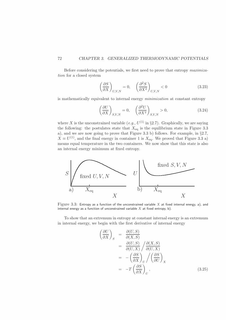
72 CHAPTER 3. GENERALIZED THERMODYNAMIC POTENTIALS
Before considering the potentials, we first need to prove that entropy maximiza-tion for a closed system
(∂S
∂X
)
U,V,N
= 0,
(∂2S
∂X2
)
U,V,N
< 0 (3.23)
is mathematically equivalent to internal energy minimization at constant entropy
(∂U
∂X
)
S,V,N
= 0,
(∂2U
∂X2
)
S,V,N
> 0, (3.24)
where X is the unconstrained variable (e.g., U (1) in §2.7). Graphically, we are sayingthe following: the postulates state that Xeq is the equilibrium state in Figure 3.3a), and we are now going to prove that Figure 3.3 b) follows. For example, in §2.7,X ≡ U (1), and the final energy in container 1 is Xeq. We proved that Figure 3.3 a)means equal temperature in the two containers. We now show that this state is alsoan internal energy minimum at fixed entropy.
Xeq
S
X
fixed U, V,N
a) Xeq
U
X
fixed S, V,N
b)
Figure 3.3: Entropy as a function of the unconstrained variable X at fixed internal energy, a), andinternal energy as a function of unconstrained variable X at fixed entropy, b).
To show that an extremum in entropy at constant internal energy is an extremumin internal energy, we begin with the first derivative of internal energy
(∂U
∂X
)
S
=∂(U,S)
∂(X,S)
=∂(U,S)
∂(U,X)
/∂(X,S)
∂(U,X)
= −(∂S
∂X
)
U
/(∂S
∂U
)
X
= −T(∂S
∂X
)
U
, (3.25)
3.2. EXTREMA PRINCIPLES FOR THE POTENTIALS 73
where it is implied that V and N are held constant in all derivatives. Since theentropy is an extremum at equilibrium and
(∂S∂X
)
U= 0, then Eqn. (3.25) shows that
internal energy is also an extremum. To show that a maximum in S corresponds toa minimum in U , it is convenient to introduce temporarily the notation ψ :=
(∂U∂X
)
S.
Then, we can write
(∂2U
∂X2
)
S
=
(∂ψ
∂X
)
S
=∂(ψ, S)
∂(X,S)
=∂(ψ, S)
∂(X,U)
∂(X,U)
∂(X,S)
= T
[1
T
(∂ψ
∂X
)
U
−(∂S
∂X
)
U
(∂ψ
∂U
)
X
]
=
(∂ψ
∂X
)
U
, when S is maximum. (3.26)
Note that the second Jacobian on the third line is just T . We expand out thedeterminant of the first one to get the fourth line. The last line follows because weare considering the state where S is a maximum, so
(∂S∂X
)
U= 0. To finish the proof,
we insert the definition of ψ into the last line above, and use Eqn. (3.25) to obtain
(∂2U
∂X2
)
S
=
(∂
∂X
(∂U
∂X
)
S
)
U
= −T(∂2S
∂X2
)
U
−(∂S
∂X
)
U
(∂T
∂X
)
U
= −T(∂2S
∂X2
)
U
, when S is maximum. (3.27)
We used Eqn. (3.25) to obtain the second line, and the fact that entropy is anextremum to obtain the last line. Eqn. (3.27) shows that when S is maximized fora closed system, internal energy is minimized at constant entropy.
To characterize the potentials, we think about how to make a process isother-mal in practice. We do this by splitting an isolated system into our subsystem ofinterest and the rest of the isolated system that we call a heat reservoir, which isat temperature Tres. The subsystem of interest and the heat reservoir are not inmechanical contact (i.e., the pressure is not necessarily the same as the pressure inthe reservoir, and dVres = dVsys = 0). A heat reservoir is a large subsystem whosetemperature cannot be changed appreciably by the interactions with the subsystem
74 CHAPTER 3. GENERALIZED THERMODYNAMIC POTENTIALS
of interest. For example, a reaction taking place in a single living cell in the humanbody might be a reasonable approximation of a system (the cell) in contact with aheat reservoir (the body). From now on we call this subsystem of interest simplythe system. We show that the equilibrium state of the system is an extremum inthe Helmholtz potential of the system only .
Since the system is at equilibrium, we know from Eqn. (2.69) that the temper-ature of the system is Tsys = Tres. From our postulates, we have proven that anequilibrium state is determined by the minimization of U at constant S, Eqn. (3.24).Since internal energy is extensive, we can write for our combined system plus reser-voir
0 =
(∂U
∂X
)
S,V,N
,
=
(∂U sys
∂X
)
S,V,N
+
(∂U res
∂X
)
S,V,N
=
(∂U sys
∂X
)
S,V,N
+ T res
(∂Sres
∂X
)
S,V,N
− P
(∂V res
∂X
)
S,V,N
+ µ
(∂N res
∂X
)
S,V,N
,
where we have used the differential for U to obtain the third line. However, we nowuse the fact that T sys = T res is a constant, and that the mole number and volume ofthe reservoir and system must also be constants. The total system is at equilibrium,so dStot = 0, and, hence dSres = −dSsys, and we find
0 =
(∂U sys
∂X
)
T sys,V sys,Nsys
− T sys
(∂Ssys
∂X
)
T sys,V sys,Nsys
=
(∂
∂X[U sys − T sysSsys]
)
T sys,V sys,Nsys
=
(∂F sys
∂X
)
T sys,V sys,Nsys
(3.28)
The last line follows from the definition of F . In a similar way, one can prove thatthis extremum is a minimum by examining the second-order derivative of F withrespect to X.
It is worthwhile to reflect on the importance of the last result. It means that theequilibrium state of a system in contact with a temperature reservoir can be foundsimply by studying the Helmholtz potential of the system—independent of what ishappening in the reservoir .
Similarly, one can show that a system in contact with a pressure reservoir reachesequilibrium when dHsys = 0, and a system in contact with both a pressure andtemperature reservoir reaches equilibrium when dGsys = 0. In Chapter 4 we show
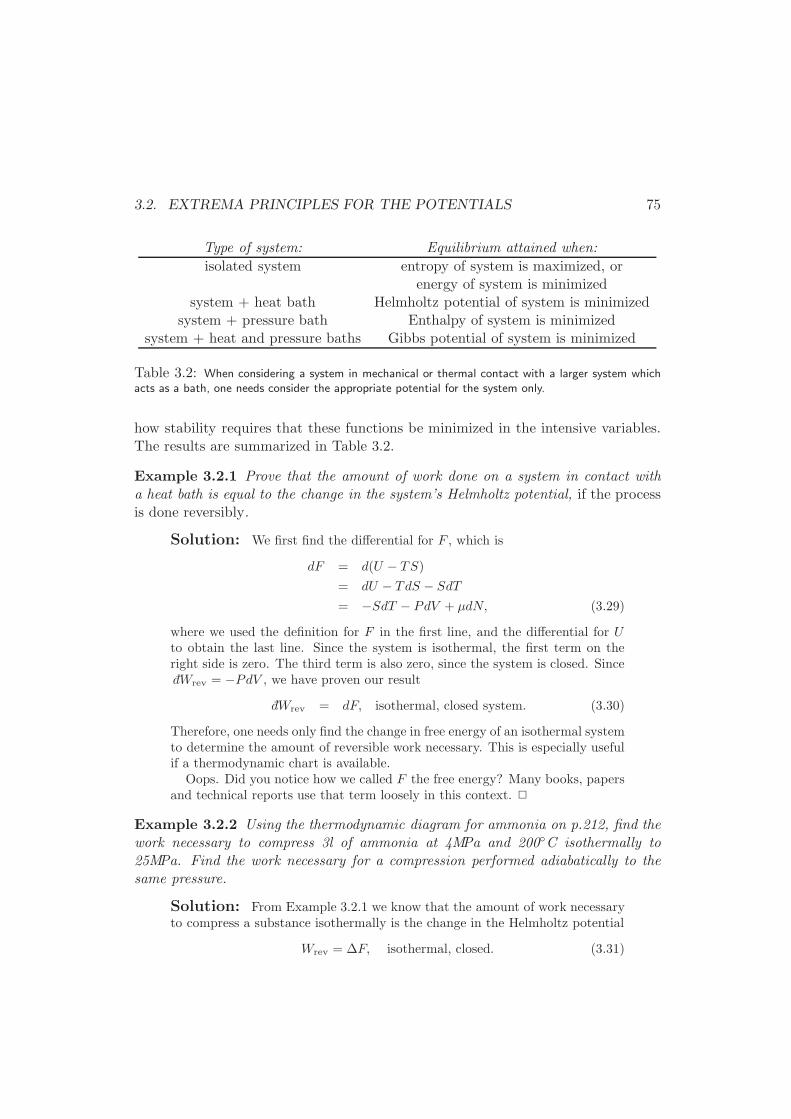
3.2. EXTREMA PRINCIPLES FOR THE POTENTIALS 75
Type of system: Equilibrium attained when:
isolated system entropy of system is maximized, orenergy of system is minimized
system + heat bath Helmholtz potential of system is minimizedsystem + pressure bath Enthalpy of system is minimized
system + heat and pressure baths Gibbs potential of system is minimized
Table 3.2: When considering a system in mechanical or thermal contact with a larger system whichacts as a bath, one needs consider the appropriate potential for the system only.
how stability requires that these functions be minimized in the intensive variables.The results are summarized in Table 3.2.
Example 3.2.1 Prove that the amount of work done on a system in contact witha heat bath is equal to the change in the system’s Helmholtz potential, if the processis done reversibly.
Solution: We first find the differential for F , which is
dF = d(U − TS)
= dU − TdS − SdT
= −SdT − PdV + µdN, (3.29)
where we used the definition for F in the first line, and the differential for Uto obtain the last line. Since the system is isothermal, the first term on theright side is zero. The third term is also zero, since the system is closed. SincedWrev = −PdV , we have proven our result
dWrev = dF, isothermal, closed system. (3.30)
Therefore, one needs only find the change in free energy of an isothermal systemto determine the amount of reversible work necessary. This is especially usefulif a thermodynamic chart is available.
Oops. Did you notice how we called F the free energy? Many books, papersand technical reports use that term loosely in this context. 2
Example 3.2.2 Using the thermodynamic diagram for ammonia on p.212, find thework necessary to compress 3l of ammonia at 4MPa and 200C isothermally to25MPa. Find the work necessary for a compression performed adiabatically to thesame pressure.
Solution: From Example 3.2.1 we know that the amount of work necessaryto compress a substance isothermally is the change in the Helmholtz potential
Wrev = ∆F, isothermal, closed. (3.31)
76 CHAPTER 3. GENERALIZED THERMODYNAMIC POTENTIALS
We see from the thermodynamic diagram, we can obtain the enthalpy, entropyand density for known temperature and pressure. This is sufficient informationto obtain the Helmholtz potential, using its definition
F := U − TS = H − PV − TS = H − PMwN
ρ− TS. (3.32)
We also used the definition of the enthalpy, and converted from volume V todensity ρ. From the diagram, we get the initial conditions
H [T = 200C,P = 4MPa] = 915.kJ/kg
S[T = 200C,P = 4MPa] = 10.55kJ/kg ·Kρ[T = 200C,P = 4MPa] = 19.kg/m
3. (3.33)
Therefore, we obtain the initial Helmholtz potential to be
fi = (915.kJ/kg)− (4× 10³kPa)(1kJ/kPa·m3)
19kg/m3 − (273 + 200K)(10.55kJ/kg·K).
= −4286.kJ/kg. (3.34)
Note that the particular choice chosen for zero enthalpy and zero entropy increating the diagram makes the Helmholtz potential negative here. The (arbi-trary) choice for zeroing internal energy cancels out when taking the difference.From the fifth postulate, we know that one cannot arbitrarily choose entropyto be zero at some state. Therefore, the values for entropy given in the diagramshould all have an additive value for S0 at the reference point. Since we take adifference here at constant temperature, this constant will vanish, so our answeris OK.
At the final state, T = 200C, P = 25MPa, we likewise find
H [T = 200C, P = 25MPa] = 430.kJ/kg
S[T = 200C, P = 25MPa] = 8.75kJ/kg·Kρ[T = 200C, P = 25MPa] = 220.kg/m3. (3.35)
Therefore, the final specific Helmholtz potential is
ff = (430.kJ/kg)− (25× 103kPa)(1kJ/kPa·m3)
220.kg/m3 − (273 + 200K)(8.75kJ/kg· K)
= −3822.kJ/kg, (3.36)
and the reversible work required is
Wrev = ∆F = ∆fN = ∆fV ρ
= (−3822.+ 4286.kJ/kg)(3l)(19.kg/m3)(10−3m3/l)
= 26.4kJ (3.37)
3.2. EXTREMA PRINCIPLES FOR THE POTENTIALS 77
Had we assumed that the gas were ideal, we would have obtained the result
WIG = −NRT log
(VfVi
)
= PiVi log
(ρfρi
)
= (4000kPa)(0.003m3)(1kJ/kPa ·m3) log
(
220.kg/m3
19.kg/m3
)
= 29.4kJ. (3.38)
Hence, the ideal gas assumption introduces an error of only 11%.To find the adiabatic compression, we recall that an adiabatic, reversible
compression is also isentropic. Hence, the final state must have Pf = 25MPa,and specific entropy equal to the initial, 10.55 kJ/kg·K. From the diagram, we
see that the final state is Tf = 395K, ρf = 80kg/m3, and hf = 1350 kJ/kg.
The required work is just the change in internal energy. From the definition ofenthalpy, we can find ui
ui = hi − Pivi = hi −Pi
ρi
= (915.kJ/kg)− 4000kPa
19.kg/m3
= 704.5kJ/kg. (3.39)
Similarly, we find the final specific internal energy to be uf = 1038 kJ/kg.Hence, the required work for the adiabatic compression is
Wadiab = ∆uN = ∆uρiVi
= (1037.5− 704.5kJ/kg)(19.kg/m3)(0.003m3)
= 19.0kJ. (3.40)
This value is smaller, because the final volume is much larger than that for theisothermal compression.2
The following example analyzes the maximum theoretical efficiency of a heat engine,which illustrates the importance of enthalpy in combustion.
Example 3.2.3 A heat engine exploits heat flowing from a hot object to a colderone. Typically, the energy is provided by burning fuel, and the environment is thecolder object. An example of such an engine is the steam cycle discussed in detailin §5.2.1. Find the maximum theoretical work available from one mole of hydrogengas as a function of temperature.
Solution: A simplified schematic of a heat engine is shown in Figure 3.4.The process is broken into two subsystems as drawn. We begin with an energy
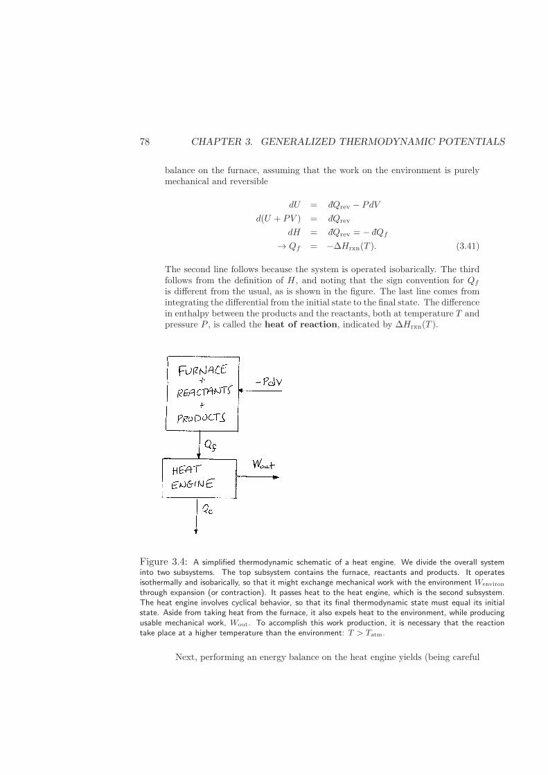
78 CHAPTER 3. GENERALIZED THERMODYNAMIC POTENTIALS
balance on the furnace, assuming that the work on the environment is purelymechanical and reversible
dU = dQrev − PdV
d(U + PV ) = dQrev
dH = dQrev = − dQf
→ Qf = −∆Hrxn(T ). (3.41)
The second line follows because the system is operated isobarically. The thirdfollows from the definition of H , and noting that the sign convention for Qfis different from the usual, as is shown in the figure. The last line comes fromintegrating the differential from the initial state to the final state. The differencein enthalpy between the products and the reactants, both at temperature T andpressure P , is called the heat of reaction, indicated by ∆Hrxn(T ).
Figure 3.4: A simplified thermodynamic schematic of a heat engine. We divide the overall systeminto two subsystems. The top subsystem contains the furnace, reactants and products. It operatesisothermally and isobarically, so that it might exchange mechanical work with the environment Wenviron
through expansion (or contraction). It passes heat to the heat engine, which is the second subsystem.The heat engine involves cyclical behavior, so that its final thermodynamic state must equal its initialstate. Aside from taking heat from the furnace, it also expels heat to the environment, while producingusable mechanical work, Wout. To accomplish this work production, it is necessary that the reactiontake place at a higher temperature than the environment: T > Tatm.
Next, performing an energy balance on the heat engine yields (being careful
3.2. EXTREMA PRINCIPLES FOR THE POTENTIALS 79
with the proper signs for heat and work flows, as shown in the drawing)
dU = dQf − dQc − dWout
(3.42)
We can integrate this equation from the initial to the final state. Since theengine operates as a cycle, its final internal energy must be the same as itsfinal, making the left side zero. Hence,
Wout = Qf −Qc = −∆Hrxn(T )−Qc,
(3.43)
where we have used the result from the energy balance on the furnace, Eqn. (3.41).To finish, we need to find the heat flow Qc. Clearly, the smaller Qc, the more
work will be available. The limitation in Qc comes from an overall entropy bal-ance. Here we perform an entropy balance over just the heat engine, assumingreversible heat transfer with its environment. The entropy balance is then
dStotal = dSenviron + dSengine, (3.44)
where the subscripts are ‘total’ for the universe, ‘environ’ for the environment,and ‘engine’ for the engine. Still assuming reversibility, we know the change inentropy for the environment from heat flow is dQc/Tatm − dQf/T . Note thatthe arrows in the sketch determine our signs here, and that we assume the heatdelivered from the furnace is at temperature T . We thus obtain
0 = − dQfT
+dQcTatm
+ dSengine, (3.45)
assuming reversibility. We integrate this equation noting that the temperaturesare constant
0 =QcTatm
− QfT, (3.46)
where we have again exploited the fact that the engine operates as a cycle. Wecan now find the amount of work available for the heat engine
Wout = (−∆Hrxn(T ))
(
1− TatmT
)
(3.47)
While we assumed that the reaction was exothermic above, this expressionactually holds for an endothermic reaction as well. In that case, each termin the parentheses is negative, and work is still available. Also note that thegreater the temperature differences, the larger the available work.
These results require that the entire system operates reversibly. Hence, en-tropy may not be generated from heat flow across finite temperature differences,all processes must be quasi-static, there is no friction, etc. Of course, real pro-cesses always operate irreversibly. So these results allow one to estimate how
80 CHAPTER 3. GENERALIZED THERMODYNAMIC POTENTIALS
close a real system is to ideal performance, or to get rough estimates whendesigning.
Also, many cyclical engines do not operate in this manner. An automobileengine, for example, exploits the expansion of the reaction of fuel to producework, rather than exploiting heat flow. Hence, the analysis done here does notapply to typical combustion engines. 2
3.3 Maxwell Relations
In the last section, we saw that the enthalpy, H, the Helmholtz potential, F , andthe Gibbs free energy, G, contain complete thermodynamic information when ex-pressed in their canonical independent variables. In Chapter 2, from the definitionsof temperature, pressure and chemical potential, we have already found the totaldifferentials for both internal energy and entropy, Eqs. (2.27) and (2.29). By simplemanipulation we found the total differential for the Helmholtz potential in Example3.2.1
dF = dU − TdS − SdT
= −SdT − PdV +
m∑
i
µidNi,
where we used the differential for internal energy Eqn. (2.27) to obtain the secondline. We can perform similar manipulations on the other potentials to find theirtotal differentials. The results are
dU = TdS − PdV +∑
i
µidNi, (3.48)
dH = TdS + V dP +∑
i
µidNi, (3.49)
dF = −SdT − PdV +∑
i
µidNi, (3.50)
dG = −SdT + V dP +∑
i
µidNi. (3.51)
From these differential expressions we can also see how to find equations of statefrom the generalized potential. In addition to those shown in the second column ofTable 3.1, we can write
T =
(∂H
∂S
)
P,N
, P = −(∂F
∂V
)
T,N
. (3.52)
3.3. MAXWELL RELATIONS 81
Therefore, all thermodynamic information can be retrieved from the generalizedpotentials as functions of their canonical variables, just as we have already donefrom the fundamental energy relation.
We can also derive some other useful, general relations, called Maxwell Rela-tions. Since H,F and G are constructed from simple manipulations of the analyticfunction U , they are also analytic (§A.1). As analytic functions, their second-orderderivatives must be independent of the order of differentiation. Hence, we can write
∂2H
∂S∂P=
∂2H
∂P∂S. (3.53)
Recall from the appendix that we must be careful to remember what independentvariables are being held constant in second-order partial derivatives. Writing theterm on the left side more explicitly and using Eqn. (3.49) we can write
∂2H
∂S∂P=
(
∂
∂S
(∂H
∂P
)
S,N
)
P,N
=
(∂V
∂S
)
P,N
. (3.54)
Similarly,
∂2H
∂P∂S=
(
∂
∂P
(∂H
∂S
)
P,N
)
S,N
=
(∂T
∂P
)
S,N
. (3.55)
Putting Eqs. (3.54) and (3.55) into Eqn. (3.53) yields our first Maxwell relation
(∂V
∂S
)
P,N
=
(∂T
∂P
)
S,N
.
Of course, we can use the same procedure for U,F and G to obtain three morerelations. When we do, we find the four Maxwell relations
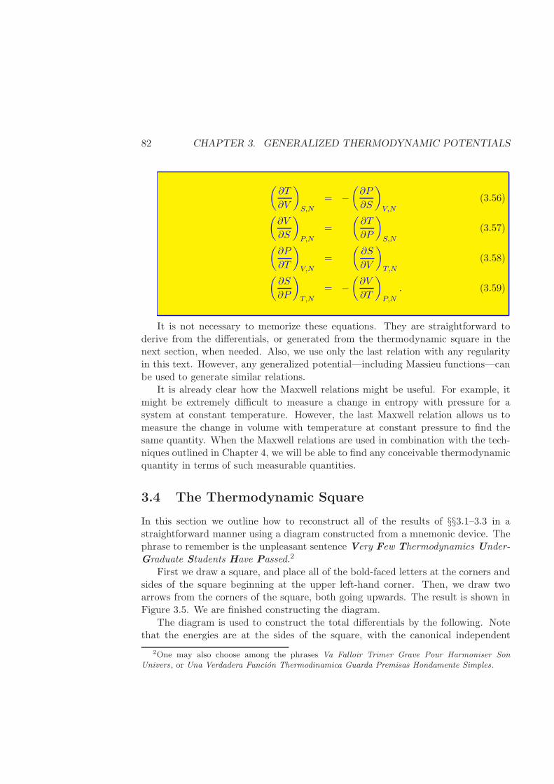
82 CHAPTER 3. GENERALIZED THERMODYNAMIC POTENTIALS
(∂T
∂V
)
S,N
= −(∂P
∂S
)
V,N
(3.56)
(∂V
∂S
)
P,N
=
(∂T
∂P
)
S,N
(3.57)
(∂P
∂T
)
V,N
=
(∂S
∂V
)
T,N
(3.58)
(∂S
∂P
)
T,N
= −(∂V
∂T
)
P,N
. (3.59)
It is not necessary to memorize these equations. They are straightforward toderive from the differentials, or generated from the thermodynamic square in thenext section, when needed. Also, we use only the last relation with any regularityin this text. However, any generalized potential—including Massieu functions—canbe used to generate similar relations.
It is already clear how the Maxwell relations might be useful. For example, itmight be extremely difficult to measure a change in entropy with pressure for asystem at constant temperature. However, the last Maxwell relation allows us tomeasure the change in volume with temperature at constant pressure to find thesame quantity. When the Maxwell relations are used in combination with the tech-niques outlined in Chapter 4, we will be able to find any conceivable thermodynamicquantity in terms of such measurable quantities.
3.4 The Thermodynamic Square
In this section we outline how to reconstruct all of the results of §§3.1–3.3 in astraightforward manner using a diagram constructed from a mnemonic device. Thephrase to remember is the unpleasant sentence Very Few Thermodynamics Under-Graduate Students Have Passed.2
First we draw a square, and place all of the bold-faced letters at the corners andsides of the square beginning at the upper left-hand corner. Then, we draw twoarrows from the corners of the square, both going upwards. The result is shown inFigure 3.5. We are finished constructing the diagram.
The diagram is used to construct the total differentials by the following. Notethat the energies are at the sides of the square, with the canonical independent
2One may also choose among the phrases Va Falloir Trimer Grave Pour Harmoniser Son
Univers, or Una Verdadera Funcion Thermodinamica Guarda Premisas Hondamente Simples.
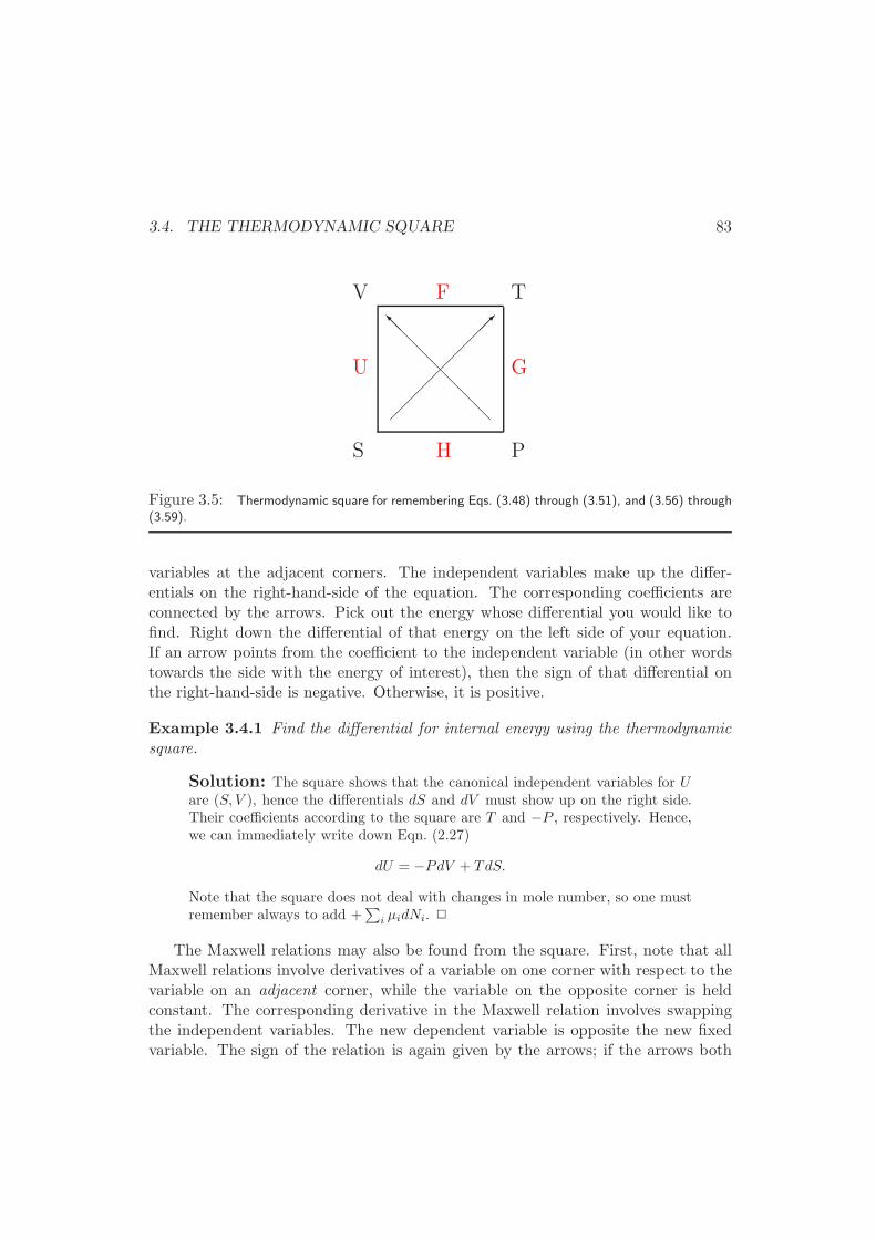
3.4. THE THERMODYNAMIC SQUARE 83
S H P
U
V
G
TF
@@
@@
@@
@@I
Figure 3.5: Thermodynamic square for remembering Eqs. (3.48) through (3.51), and (3.56) through(3.59).
variables at the adjacent corners. The independent variables make up the differ-entials on the right-hand-side of the equation. The corresponding coefficients areconnected by the arrows. Pick out the energy whose differential you would like tofind. Right down the differential of that energy on the left side of your equation.If an arrow points from the coefficient to the independent variable (in other wordstowards the side with the energy of interest), then the sign of that differential onthe right-hand-side is negative. Otherwise, it is positive.
Example 3.4.1 Find the differential for internal energy using the thermodynamicsquare.
Solution: The square shows that the canonical independent variables for Uare (S, V ), hence the differentials dS and dV must show up on the right side.Their coefficients according to the square are T and −P , respectively. Hence,we can immediately write down Eqn. (2.27)
dU = −PdV + TdS.
Note that the square does not deal with changes in mole number, so one mustremember always to add +
∑
i µidNi. 2
The Maxwell relations may also be found from the square. First, note that allMaxwell relations involve derivatives of a variable on one corner with respect to thevariable on an adjacent corner, while the variable on the opposite corner is heldconstant. The corresponding derivative in the Maxwell relation involves swappingthe independent variables. The new dependent variable is opposite the new fixedvariable. The sign of the relation is again given by the arrows; if the arrows both
84 CHAPTER 3. GENERALIZED THERMODYNAMIC POTENTIALS
point to (or both point away from) the dependent variables, the sign is positive. Ifone arrow points towards one of the dependent variables, but the other arrow pointsaway from the other dependent variables, the sign is negative.
Example 3.4.2 Find a Maxwell relation for(∂S∂V
)
T.
Solution: We note that the fixed variable T lies opposite to the dependentvariable S, and that the independent variable V lies adjacent to S, so thereexists a Maxwell relation for the derivative.
The differential related to this one by a Maxwell relation must have V as thefixed variable, and T as the changing variable. The intensive variable oppositeV must be the dependent variable, or P . Hence, our second differential is
(∂P
∂T
)
V
.
Both arrows point away from the dependent variables S and P , so the signmust be the same on each. Hence, we have just found Eqn. (3.58) using thethermodynamic square. 2
It is highly recommended that the reader attempt to reconstruct all of the dif-ferentials and the Maxwell relations with a blank sheet of paper, a pencil, andremembering that very few thermodynamics undergraduate students have passed.
3.5 Coefficient of Thermal Expansion, Isothermal Com-pressibility and Constant-Pressure Heat Capacity
Everyday experience shows that many material properties are functions of the first-order derivatives T, P, and µi. For example, when objects become warmer, theirvolume increases. Gases and liquids can shrink considerably under an increase ofpressure, and ice freezes at a lower temperature when the chemical potential of saltin the ice is increased. These effects are all examples of second-order derivatives.3
The three most frequently tabulated second-order derivatives for pure substancesare
3Since pressure and temperature are first-order derivatives of the fundamental variableU(S, V,N), we call quantities that are derivatives of these second-order derivatives.
3.5. SECOND-ORDER COEFFICIENTS 85
α :=1
v
(∂v
∂T
)
P
, “coefficient of thermal expansion” (3.60)
κT := −1
v
(∂v
∂P
)
T
, “isothermal compressibility” (3.61)
cP := T
(∂s
∂T
)
P
, “constant-pressure heat capacity” (3.62)
These definitions should be memorized. Using the thermodynamic transforma-tions introduced in §3.6, it is possible to relate all other second-order derivatives tothese three. These quantities can be found from measurement, tables, or equationsof state like those given in §§B and D.2. It is straightforward to imagine experimentsto measure α or κT . To measure CP , we use Eqn. (2.46) to write
CP := T
(∂S
∂T
)
P
=
(∂Qqs
∂T
)
P
. (3.63)
Therefore, if one has information on how much heat is required to raise the tem-perature of a substance by a small amount at constant pressure, the ratio of heatdivided by temperature change is the heat capacity. Such measurements are rou-tinely performed in a differential scanning calorimeter, or DSC. These devicesraise the temperature of a substance at a controlled rate, and measure the rate ofheat required for the change. If these rates are sufficiently slow that the process isquasi-static, then the ratio of d
dtQ to ddtT yields the heat capacity as a function of
temperature.4
As an aside, we point out that intuitively we expect each of these quantities tobe positive. In fact, that is how the signs were chosen for the definitions. In §4.1 wewill see that the postulates indeed show that κT and cP are required to be positive.
Example 3.5.1 Find the isothermal compressibility for the simple van der Waalsfluid.
Solution: From Examples 2.5.1 and 2.6.1, we have seen that the proposedfundamental entropy relation given in Eqn. (2.21) leads to the van der Waalsmechanical equation of state
P =RT
V/N − b− aN2
V 2, (2.35)
4Glassy liquids are ones that relax extremely slowly, and can fall out of equilibrium upon cooling.Hence, most DSCs change the temperature too fast to be quasi-static for these, and spurious resultscan be obtained.
86 CHAPTER 3. GENERALIZED THERMODYNAMIC POTENTIALS
and the simple van der Waals thermal equation of state Eqn. (2.34). We beginwith the definition of κT Eqn. (3.61)
κT := −1
v
(∂v
∂P
)
T
= − 1
v(∂P∂v
)
T
=v2 (v − b)2
RTv3 − 2a (v − b)2 . (3.64)
To obtain the second line we applied the relation Eqn. (A.18). Then, in orderto find the derivative in the denominator, we take the derivative of each side ofthe van der Waals mechanical equation of state (2.35) with respect to v, andinsert the result into the second line above. After some algebraic manipulation,the third line is the result.
Note that the denominator can pass through zero for some values of v. Thismeans that the van der Waals fluid’s isothermal compressibility can sometimesbe infinity! Is this result physical? The surprising answer to this question mustwait until the next chapter. 2
Example 3.5.2 Find the constant-pressure and constant-volume heat capacities forthe general ideal gas given in Example 3.1.2.
Solution: The definition for the constant-pressure heat capacity Eqn. (3.62)requires that we have s(T, P ). However, Eqn. (3.17) gives entropy as a functionof temperature and volume. If we use the ideal gas law found in Example 3.1.3to eliminate volume from Eqn. (3.17), we obtain
S = Ns0 +N
∫ T
T0
cidealv (T ′)
T ′dT ′ +NR log
[RT
Pv0
]
,
general ideal gas. (3.65)
Inserting this expression into the definition Eqn. (3.62) gives us the constant-pressure heat capacity for the general ideal gas described by Eqn. (3.16)
cP (T ) = R+ cidealv (T ), general ideal gas.
Note that it was necessary to use the Leibniz rule Eqn. (A.25) to obtain thisresult.
The constant-volume heat capacity has the logical definition
cV := T
(∂s
∂T
)
v
, (3.66)
which, when applied to Eqn. (3.65) shows that the function “cidealv (T )” is aptlynamed. 2

3.5. SECOND-ORDER COEFFICIENTS 87
cidealv (T ) is actually called the “ideal constant-volume heat capacity.” Polynomialexpressions for several pure-component substances are given in Table D.2.
The second-order derivatives are extremely useful for solving problems. In thefollowing example, we show how to extract the work available from a hydrogen fuelcell, which operates isothermally and isobarically using the heat capacity, and aresult from §3.2.
Example 3.5.3 Prove that the amount of electrical work available from a fuel cellis equal to the change in the system’s Gibbs potential, if the process is done isother-mally, isobarically, and reversibly. Use these results to find the maximum workavailable from a hydrogen fuel cell utilizing the reaction
H2 +1
2O2 → H2O(g),
for 300K < T < 1000K.
Solution: A fuel cell takes reactants (e.g., hydrogen and oxygen) and reactsthem to make electricity. Figure 3.6 shows a picture of a fuel cell, and Figure 3.7shows a schematic of its operation. The oxidation reaction and the reductionreaction take place at different electrodes, and the transport of the electronstakes place not through the liquid phase, but rather through an electrical circuit.The circuit can then extract the work available from the reaction.
These systems are open, since reactants and products flow through the fuelcell. However, we will simplify the system by looking at the final state (theproducts + fuel cell), the initial state (the reactants + fuel cell), the workdone, and the heat flow. The system is still open, however, since electrons flowacross the system boundary, providing the electrical work (Figure 3.8).
For our system, we begin with the conservation-of-energy equation
dU = dQ + dW. (2.1)
For our system, there are two possible kinds of work: mechanical (from compres-sion or expansion), and electrical work. We are assuming here that everythinghappens reversibly. It is important to note here that we have written the elec-trical work as positive in Figure 3.8 when it provides work to the surroundings.
We begin with the differential for internal energy
dU = TdS − PdV +∑
i
µidNi
= TdS − PdV + µine dN
ine + µout
e dNoute ,
= TdS − PdV +(µine − µout
e
)dN in
e , (3.67)
since only the electrons cross the boundary, and the electrons entering oneelectrode must balance those exiting the other. Clearly, the first term on the
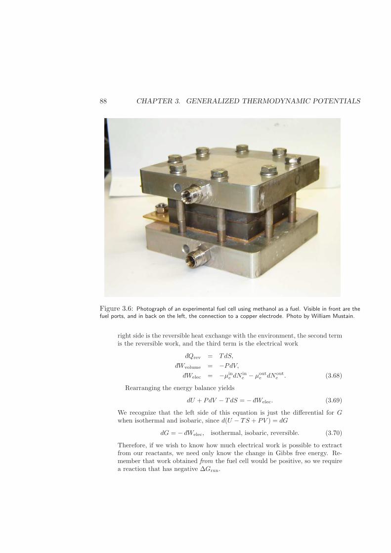
88 CHAPTER 3. GENERALIZED THERMODYNAMIC POTENTIALS
Figure 3.6: Photograph of an experimental fuel cell using methanol as a fuel. Visible in front are thefuel ports, and in back on the left, the connection to a copper electrode. Photo by William Mustain.
right side is the reversible heat exchange with the environment, the second termis the reversible work, and the third term is the electrical work
dQrev = TdS,
dWvolume = −PdV,dWelec = −µin
e dNine − µout
e dNoute . (3.68)
Rearranging the energy balance yields
dU + PdV − TdS = − dWelec. (3.69)
We recognize that the left side of this equation is just the differential for Gwhen isothermal and isobaric, since d(U − TS + PV ) = dG
dG = − dWelec, isothermal, isobaric, reversible. (3.70)
Therefore, if we wish to know how much electrical work is possible to extractfrom our reactants, we need only know the change in Gibbs free energy. Re-member that work obtained from the fuel cell would be positive, so we requirea reaction that has negative ∆Grxn.
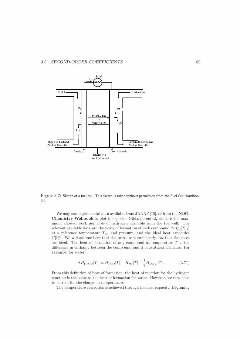
3.5. SECOND-ORDER COEFFICIENTS 89
Figure 3.7: Sketch of a fuel cell. This sketch is taken without permission from the Fuel Cell Handbook[3].
Wemay use experimental data available from JANAF [15], or from theNISTChemistry Webbook to plot the specific Gibbs potential, which is the max-imum allowed work per mole of hydrogen available from the fuel cell. Therelevant available data are the heats of formation of each compound ∆H
f,i[Tref ]at a reference temperature Tref and pressure, and the ideal heat capacitiesC idealP,i . We will assume here that the pressure is sufficiently low that the gases
are ideal. The heat of formation of any compound at temperature T is thedifference in enthalpy between the compound and it constituent elements. Forexample, for water
∆Hf,H2O[T ] := HH2O[T ]−HH2 [T ]−1
2HO2(g)[T ]. (3.71)
From this definition of heat of formation, the heat of reaction for the hydrogenreaction is the same as the heat of formation for water. However, we now needto correct for the change in temperature.
The temperature correction is achieved through the heat capacity. Beginning
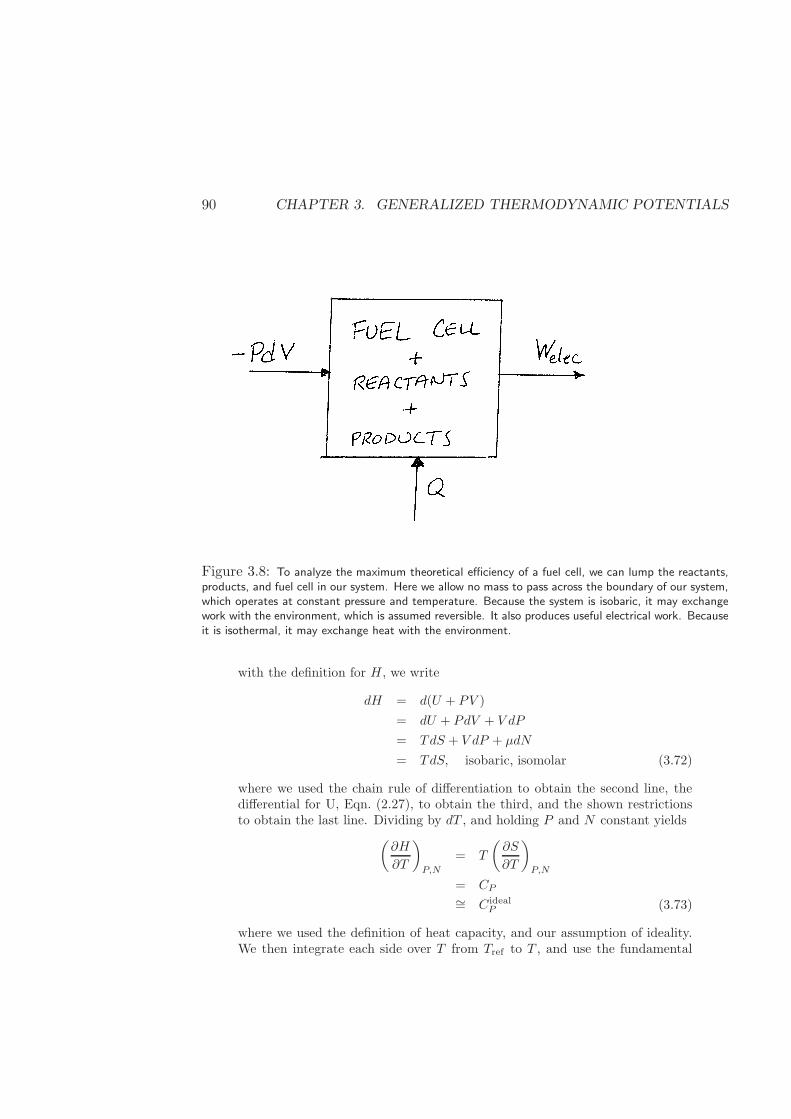
90 CHAPTER 3. GENERALIZED THERMODYNAMIC POTENTIALS
Figure 3.8: To analyze the maximum theoretical efficiency of a fuel cell, we can lump the reactants,products, and fuel cell in our system. Here we allow no mass to pass across the boundary of our system,which operates at constant pressure and temperature. Because the system is isobaric, it may exchangework with the environment, which is assumed reversible. It also produces useful electrical work. Becauseit is isothermal, it may exchange heat with the environment.
with the definition for H , we write
dH = d(U + PV )
= dU + PdV + V dP
= TdS + V dP + µdN
= TdS, isobaric, isomolar (3.72)
where we used the chain rule of differentiation to obtain the second line, thedifferential for U, Eqn. (2.27), to obtain the third, and the shown restrictionsto obtain the last line. Dividing by dT , and holding P and N constant yields
(∂H
∂T
)
P,N
= T
(∂S
∂T
)
P,N
= CP∼= C ideal
P (3.73)
where we used the definition of heat capacity, and our assumption of ideality.We then integrate each side over T from Tref to T , and use the fundamental
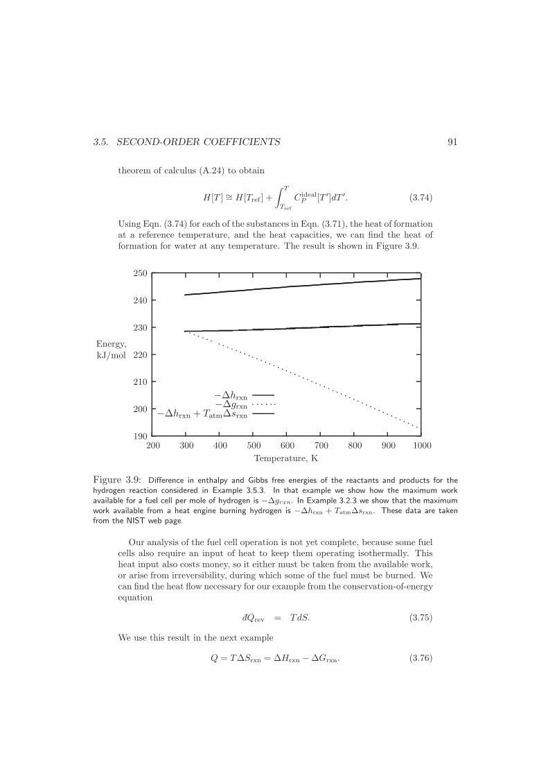
3.5. SECOND-ORDER COEFFICIENTS 91
theorem of calculus (A.24) to obtain
H [T ] ∼= H [Tref ] +
∫ T
Tref
C idealP [T ′]dT ′. (3.74)
Using Eqn. (3.74) for each of the substances in Eqn. (3.71), the heat of formationat a reference temperature, and the heat capacities, we can find the heat offormation for water at any temperature. The result is shown in Figure 3.9.
190
200
210
220
230
240
250
200 300 400 500 600 700 800 900 1000
Energy,kJ/mol
Temperature, K
−∆hrxn−∆grxn−∆hrxn + Tatm∆srxn
Figure 3.9: Difference in enthalpy and Gibbs free energies of the reactants and products for thehydrogen reaction considered in Example 3.5.3. In that example we show how the maximum workavailable for a fuel cell per mole of hydrogen is −∆grxn. In Example 3.2.3 we show that the maximumwork available from a heat engine burning hydrogen is −∆hrxn + Tatm∆srxn. These data are takenfrom the NIST web page.
Our analysis of the fuel cell operation is not yet complete, because some fuelcells also require an input of heat to keep them operating isothermally. Thisheat input also costs money, so it either must be taken from the available work,or arise from irreversibility, during which some of the fuel must be burned. Wecan find the heat flow necessary for our example from the conservation-of-energyequation
dQrev = TdS. (3.75)
We use this result in the next example
Q = T∆Srxn = ∆Hrxn −∆Grxn. (3.76)
92 CHAPTER 3. GENERALIZED THERMODYNAMIC POTENTIALS
Figure 3.9 shows that ∆Grxn > ∆Hrxn. Therefore, Q < 0, and heat flows outof the hydrogen fuel cell. Since, at these temperatures, the fuel cell is operatingabove room temperature, there is no additional cost of heating or refrigerating.In Figure 3.9 we also show the maximum theoretical work possible for a heatengine that burns hydrogen, assuming Tatm = 298K. We see that the heatengine has a higher theoretical efficiency, but only if there is an extremely coldreservoir to expel the heat. 2
In the previous example, we found the maximum electrical work available from ahydrogen fuel cell operating isothermally and isobarically at a range of temperatures.Fuel cells are sometimes touted as having greater theoretical efficiency than heatengines. Applying the results of the last examples to Example 3.2.3, we can thenfind the conditions where work available from a fuel cell is greater than work availablefrom a heat engine for the same amount of fuel. This comparison is made in thenext example.
Example 3.5.4 When does a fuel cell have a higher theoretical efficiency than aheat engine for a given reaction?
Solution: In Example 3.5.3, we analyzed a hydrogen fuel cell. From thatanalysis we discovered that the fuel cell expelled heat to its environment. Sincethe fuel cell was operating at temperatures well above ambient, this incurredno more cost. However, if the fuel cell required energy to maintain its constanttemperature, or if it operated at lower temperatures, the answer would bedifferent. Therefore, several possible outcomes are possible for the comparison.
First of all, however, the fuel cell and heat engine both require that ∆Grxn <0, or the reaction will not take place (see Table 3.2). On the other hand, ∆Srxn
can be positive or negative. Also, knowledge of the operating temperaturerelative to ambient temperature Tatm is important to determine whether wemust incur the costs of heating or cooling the fuel cell. We consider the resultingfour cases one at a time.
1. ∆Srxn > 0 and T > Tatm.
Since ∆Srxn > 0, the heat into the fuel cell Q = T∆Srxn > 0 is positive.Since the temperature of the cell is above ambient, it requires heat tomaintain its temperature, Eqn. (3.75).
To continue the comparison, we make a simplifying assumption that someamount of the fuel is burned outside of the fuel cell to supply the heat. Letus find the amount of fuel that would be burned. For every mole of fuel,x reacted in the cell, 1− x is burned to keep the cell warm. The amountof heat necessary to warm the cell per mole of fuel is Q/N = xT∆srxnfrom Eqn. (3.76). The heat available from burning the 1−x moles of fuelis Q = −∆hrxn(1− x). Setting these two expressions for Q equal tells us
3.5. SECOND-ORDER COEFFICIENTS 93
what fraction of fuel must be burned to keep the cell operating
x =∆Hrxn
∆Grxn. (3.77)
Therefore, the amount of work available is
Welec = −x∆Grxn = −∆Hrxn
∆Grxn∆Grxn = −∆Hrxn. (3.78)
Hence, the fuel cell has the same theoretical maximum of work as a heatengine, but only if there exists a heat reservoir at zero temperature.
In reality, the inefficiency of a fuel cell probably generates heat, reducing xin our analysis, but simultaneously reducing W . At any rate, the analysishere is the theoretical maximum.
2. ∆Srxn > 0 and T < Tatm.
Here, the fuel cell still requires heat. However, since it operates belowambient temperature, no fuel must be burned, and heat can be absorbedfrom the environment. Also, since ∆Srxn > 0,
Welec = −∆Grxn > −∆Hrxn, (3.79)
and the fuel cell has a higher maximum theoretical efficiency than a heatengine. In practice, existing fuel cells all operate at elevated temperatures,so this advantage is not exploited. The elevated temperature is requiredfor a practical reason: faster kinetics. In theory, a fuel cell could bedesigned to be more efficient than a heat engine at low temperatures.
3. ∆Srxn < 0 and T > Tatm.
For this case, Q < 0, and heat is dissipated to the environment. Since thefuel cell is hotter than the environment, no additional cost is incurred forcooling. Therefore, the available work is
Welec = −∆Grxn < −∆Hrxn, (3.80)
and the fuel cell has less available work than a heat engine. A real compar-ison requires knowing the reaction and ambient temperatures, however.
4. ∆Srxn < 0 and T < Tatm.
The fuel cell still expels heat, but now it will not flow to the environment,except perhaps using a refrigerator, which costs money. This is the worstcase of all. Not only is −∆Grxn < −∆Hrxn, we do not even get all of thework from −∆Grxn, because we have to pay for a refrigerator.
A summary of these results is shown in Table 3.3. Currently, all fuel cellsoperate at temperatures well above ambient, so only cases 1 and 3 aretypical. The hydrogen fuel cell considered in Example 3.5.3 is a specialcase of the second line of Table 3.3. In Problem 3.3.F. we consider amethanol fuel cell, which is described by the first line of the table.
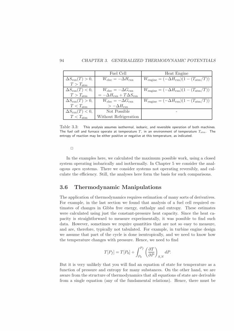
94 CHAPTER 3. GENERALIZED THERMODYNAMIC POTENTIALS
Fuel Cell Heat Engine
∆Srxn(T ) > 0, Welec = −∆Hrxn Wengine = (−∆Hrxn)(1 − (Tatm/T ))T > Tatm
∆Srxn(T ) < 0, Welec = −∆Grxn Wengine = (−∆Hrxn)(1 − (Tatm/T ))T > Tatm = −∆Hrxn + T∆Srxn
∆Srxn(T ) > 0, Welec = −∆Grxn Wengine = (−∆Hrxn)(1 − (Tatm/T ))T < Tatm > −∆Hrxn
∆Srxn(T ) < 0, Not Possible -T < Tatm Without Refrigeration
Table 3.3: This analysis assumes isothermal, isobaric, and reversible operation of both machines.The fuel cell and furnace operate at temperature T , in an environment of temperature Tatm. Theentropy of reaction may be either positive or negative at this temperature, as indicated.
2
In the examples here, we calculated the maximum possible work, using a closedsystem operating isobarically and isothermally. In Chapter 5 we consider the anal-ogous open systems. There we consider systems not operating reversibly, and cal-culate the efficiency. Still, the analyses here form the basis for such comparisons.
3.6 Thermodynamic Manipulations
The application of thermodynamics requires estimation of many sorts of derivatives.For example, in the last section we found that analysis of a fuel cell required es-timates of changes in Gibbs free energy, enthalpy and entropy. These estimateswere calculated using just the constant-pressure heat capacity. Since the heat ca-pacity is straightforward to measure experimentally, it was possible to find suchdata. However, sometimes we require quantities that are not so easy to measure,and are, therefore, typically not tabulated. For example, in turbine engine designwe assume that part of the cycle is done isentropically, and we need to know howthe temperature changes with pressure. Hence, we need to find
T [Pf ] = T [P0] +
∫ Pf
P0
(∂T
∂P
)
S,N
dP.
But it is very unlikely that you will find an equation of state for temperature as afunction of pressure and entropy for many substances. On the other hand, we areaware from the structure of thermodynamics that all equations of state are derivablefrom a single equation (any of the fundamental relations). Hence, there must be
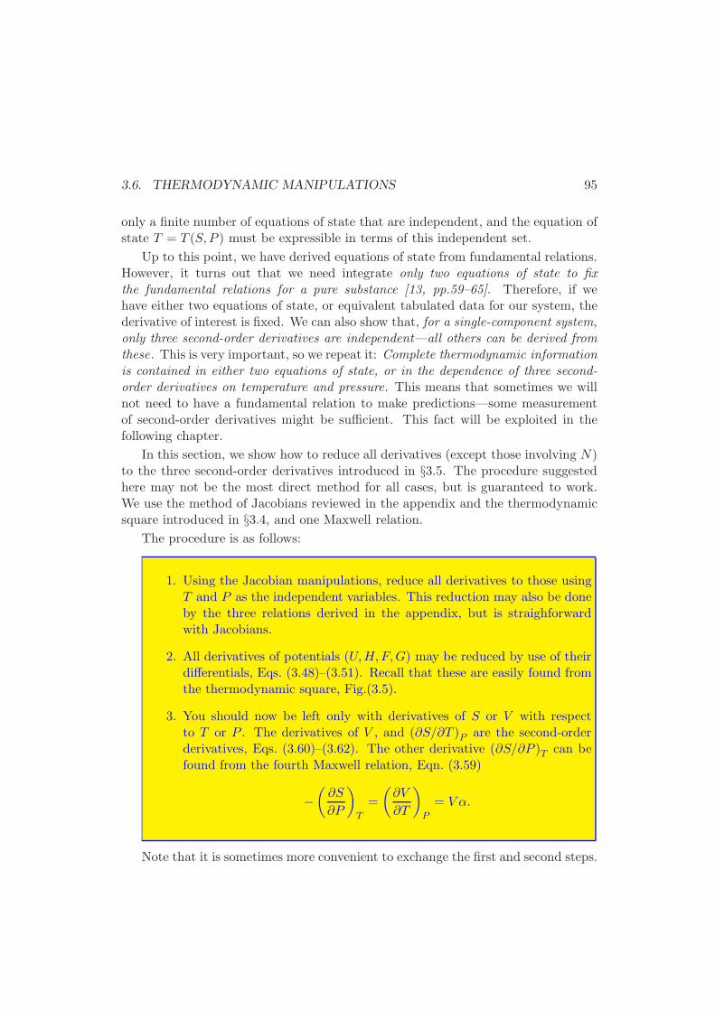
3.6. THERMODYNAMIC MANIPULATIONS 95
only a finite number of equations of state that are independent, and the equation ofstate T = T (S,P ) must be expressible in terms of this independent set.
Up to this point, we have derived equations of state from fundamental relations.However, it turns out that we need integrate only two equations of state to fixthe fundamental relations for a pure substance [13, pp.59–65]. Therefore, if wehave either two equations of state, or equivalent tabulated data for our system, thederivative of interest is fixed. We can also show that, for a single-component system,only three second-order derivatives are independent—all others can be derived fromthese. This is very important, so we repeat it: Complete thermodynamic informationis contained in either two equations of state, or in the dependence of three second-order derivatives on temperature and pressure. This means that sometimes we willnot need to have a fundamental relation to make predictions—some measurementof second-order derivatives might be sufficient. This fact will be exploited in thefollowing chapter.
In this section, we show how to reduce all derivatives (except those involving N)to the three second-order derivatives introduced in §3.5. The procedure suggestedhere may not be the most direct method for all cases, but is guaranteed to work.We use the method of Jacobians reviewed in the appendix and the thermodynamicsquare introduced in §3.4, and one Maxwell relation.
The procedure is as follows:
1. Using the Jacobian manipulations, reduce all derivatives to those usingT and P as the independent variables. This reduction may also be doneby the three relations derived in the appendix, but is straighforwardwith Jacobians.
2. All derivatives of potentials (U,H,F,G) may be reduced by use of theirdifferentials, Eqs. (3.48)–(3.51). Recall that these are easily found fromthe thermodynamic square, Fig.(3.5).
3. You should now be left only with derivatives of S or V with respectto T or P . The derivatives of V , and (∂S/∂T )P are the second-orderderivatives, Eqs. (3.60)–(3.62). The other derivative (∂S/∂P )T can befound from the fourth Maxwell relation, Eqn. (3.59)
−(∂S
∂P
)
T
=
(∂V
∂T
)
P
= V α.
Note that it is sometimes more convenient to exchange the first and second steps.
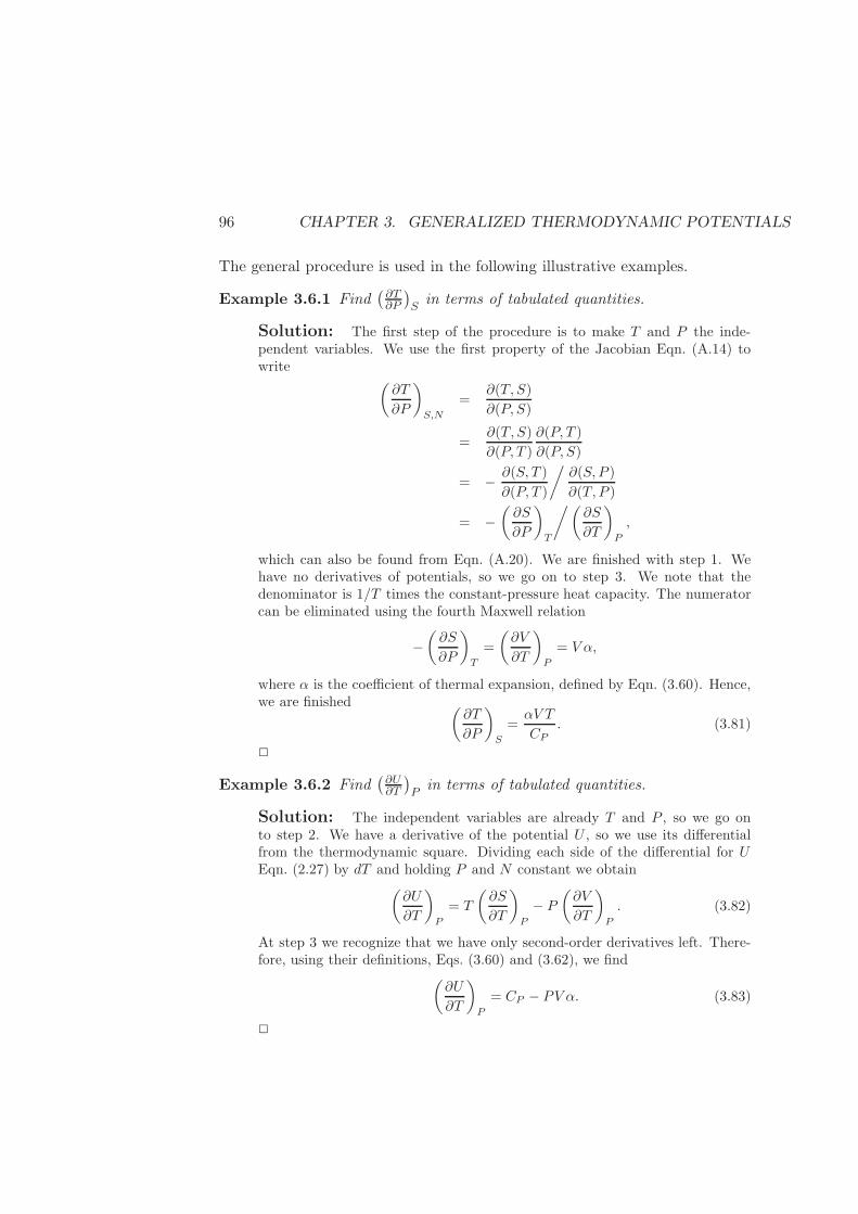
96 CHAPTER 3. GENERALIZED THERMODYNAMIC POTENTIALS
The general procedure is used in the following illustrative examples.
Example 3.6.1 Find(∂T∂P
)
Sin terms of tabulated quantities.
Solution: The first step of the procedure is to make T and P the inde-pendent variables. We use the first property of the Jacobian Eqn. (A.14) towrite
(∂T
∂P
)
S,N
=∂(T, S)
∂(P, S)
=∂(T, S)
∂(P, T )
∂(P, T )
∂(P, S)
= − ∂(S, T )
∂(P, T )
/∂(S, P )
∂(T, P )
= −(∂S
∂P
)
T
/(∂S
∂T
)
P
,
which can also be found from Eqn. (A.20). We are finished with step 1. Wehave no derivatives of potentials, so we go on to step 3. We note that thedenominator is 1/T times the constant-pressure heat capacity. The numeratorcan be eliminated using the fourth Maxwell relation
−(∂S
∂P
)
T
=
(∂V
∂T
)
P
= V α,
where α is the coefficient of thermal expansion, defined by Eqn. (3.60). Hence,we are finished (
∂T
∂P
)
S
=αV T
CP. (3.81)
2
Example 3.6.2 Find(∂U∂T
)
Pin terms of tabulated quantities.
Solution: The independent variables are already T and P , so we go onto step 2. We have a derivative of the potential U , so we use its differentialfrom the thermodynamic square. Dividing each side of the differential for UEqn. (2.27) by dT and holding P and N constant we obtain
(∂U
∂T
)
P
= T
(∂S
∂T
)
P
− P
(∂V
∂T
)
P
. (3.82)
At step 3 we recognize that we have only second-order derivatives left. There-fore, using their definitions, Eqs. (3.60) and (3.62), we find
(∂U
∂T
)
P
= CP − PV α. (3.83)
2
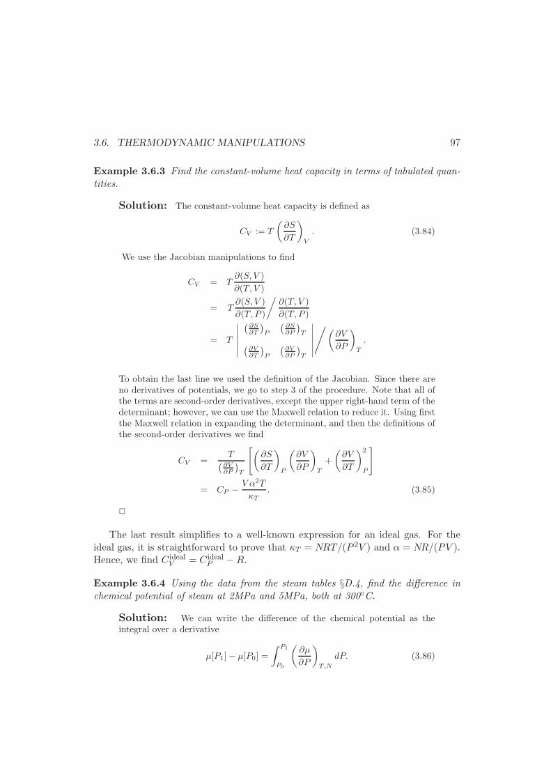
3.6. THERMODYNAMIC MANIPULATIONS 97
Example 3.6.3 Find the constant-volume heat capacity in terms of tabulated quan-tities.
Solution: The constant-volume heat capacity is defined as
CV := T
(∂S
∂T
)
V
. (3.84)
We use the Jacobian manipulations to find
CV = T∂(S, V )
∂(T, V )
= T∂(S, V )
∂(T, P )
/∂(T, V )
∂(T, P )
= T
∣∣∣∣∣∣
(∂S∂T
)
P
(∂S∂P
)
T
(∂V∂T
)
P
(∂V∂P
)
T
∣∣∣∣∣∣
/(∂V
∂P
)
T
.
To obtain the last line we used the definition of the Jacobian. Since there areno derivatives of potentials, we go to step 3 of the procedure. Note that all ofthe terms are second-order derivatives, except the upper right-hand term of thedeterminant; however, we can use the Maxwell relation to reduce it. Using firstthe Maxwell relation in expanding the determinant, and then the definitions ofthe second-order derivatives we find
CV =T
(∂V∂P
)
T
[(∂S
∂T
)
P
(∂V
∂P
)
T
+
(∂V
∂T
)2
P
]
= CP − V α2T
κT. (3.85)
2
The last result simplifies to a well-known expression for an ideal gas. For theideal gas, it is straightforward to prove that κT = NRT/(P 2V ) and α = NR/(PV ).Hence, we find C ideal
V = C idealP −R.
Example 3.6.4 Using the data from the steam tables §D.4, find the difference inchemical potential of steam at 2MPa and 5MPa, both at 300C.
Solution: We can write the difference of the chemical potential as theintegral over a derivative
µ[P1]− µ[P0] =
∫ P1
P0
(∂µ
∂P
)
T,N
dP. (3.86)
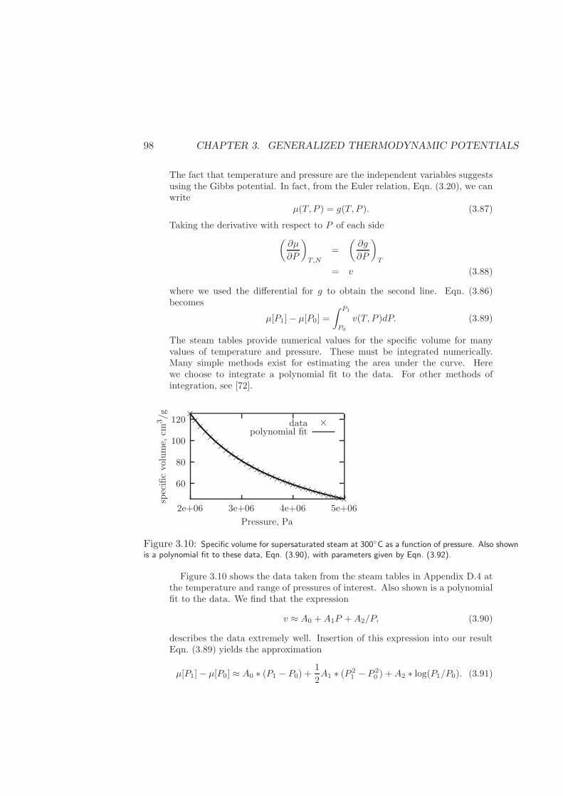
98 CHAPTER 3. GENERALIZED THERMODYNAMIC POTENTIALS
The fact that temperature and pressure are the independent variables suggestsusing the Gibbs potential. In fact, from the Euler relation, Eqn. (3.20), we canwrite
µ(T, P ) = g(T, P ). (3.87)
Taking the derivative with respect to P of each side(∂µ
∂P
)
T,N
=
(∂g
∂P
)
T
= v (3.88)
where we used the differential for g to obtain the second line. Eqn. (3.86)becomes
µ[P1]− µ[P0] =
∫ P1
P0
v(T, P )dP. (3.89)
The steam tables provide numerical values for the specific volume for manyvalues of temperature and pressure. These must be integrated numerically.Many simple methods exist for estimating the area under the curve. Herewe choose to integrate a polynomial fit to the data. For other methods ofintegration, see [72].
60
80
100
120
2e+06 3e+06 4e+06 5e+06
specificvolume,
cm3/g
Pressure, Pa
data×××××××××××××××××××××××××××××××
×polynomial fit
Figure 3.10: Specific volume for supersaturated steam at 300C as a function of pressure. Also shownis a polynomial fit to these data, Eqn. (3.90), with parameters given by Eqn. (3.92).
Figure 3.10 shows the data taken from the steam tables in Appendix D.4 atthe temperature and range of pressures of interest. Also shown is a polynomialfit to the data. We find that the expression
v ≈ A0 +A1P +A2/P, (3.90)
describes the data extremely well. Insertion of this expression into our resultEqn. (3.89) yields the approximation
µ[P1]− µ[P0] ≈ A0 ∗ (P1 − P0) +1
2A1 ∗ (P 2
1 − P 20 ) +A2 ∗ log(P1/P0). (3.91)
3.7. ONE- AND TWO-DIMENSIONAL SYSTEMS 99
Using a Levenberg-Marquardt method5 for fitting a nonlinear function todata, we obtain estimates for the parameters
A0 ≈ −5.9024cm3/g,
A1 ≈ −3.2222× 10⁻⁷cm3/g·Pa, (3.92)
A2 ≈ 2.609× 108cm3·Pa/g.
Using the fact that 1MPa·cm3 = 1J, we find that the chemical potential differ-ence is
µ[P1]− µ[P0] ≈ 217.5J/g. (3.93)
2
3.7 One- and Two-Dimensional Systems
In §2.9 we considered the fundamental entropy relation of a simple, ideal rubberband. In this section, we generalize the structure of thermodynamics a little bitmore to incorporate the generalized thermodynamic potentials introduced in thischapter. In particular, we revisit the rubber band to allow non-simple and non-ideal behavior. We also consider Langmuir adsorption isotherms to describe theattachment of molecules to adsorption sites on a solid surface. In the followingsubsection we derive our first fundamental relation from two equations of state thatare found experimentally.
3.7.1 Non-ideal Rubber Band
Experiments show that the tension in a rubber band increases linearly with tem-perature at a fixed length, for stretches greater than approximately 10% [58]. Wecan use this experimental fact to show that stretching a rubber band isothermallydecreases the entropy of the rubber band, but does not change its internal energy.We write the experimental observation as
T = Tψ(L), (3.94)
where ψ(L) is some arbitrary, but measurable function of length, such that the ten-sion is zero at the rest length L0, ψ(L0) = 0, but positive for L > L0. Since T and Lare the independent variables (the variables easily manipulated in experiment), it isnatural to use F as our fundamental relation. Using the relationship between pres-sure and Helmholtz potential implied by its differential, we can integrate Eqn. (3.94)
5See, for example [72, §15.5]. Note that a power-law expression v = A0Pa may work even better,
and is easier to fit.
100 CHAPTER 3. GENERALIZED THERMODYNAMIC POTENTIALS
from L0 to arbitrary L at constant temperature to obtain
F (T,L)− F [L0] =
∫ L
L0
(∂F
∂L
)
T
dL
=
∫ L
L0
T (T,L)dL
= T
∫ L
L0
ψ(L′)dL′. (3.95)
If we take the derivative with respect to T of each side of this equation, we canobtain an equation of state for entropy
S(T,L)− S[L0] = −∫ L
L0
ψ(L′)dL′. (3.96)
Note that the entropy decreases with stretching. We can find S[L0] from an inte-gration over temperature
S[L0] = S[T0, L0] +
∫ T
T0
(∂S
∂T
)
L
∣∣∣∣L=L0
dT
= S[T0, L0] +
∫ T
T0
CL[T′, L0]
T ′ dT ′, (3.97)
where CL := T (∂S/∂T )L is the constant-length heat capacity for the rubber band.6
Similarly, we can find F [L0] from an integration
F [L0] = F [T0, L0] +
∫ T
T0
(∂F
∂T
)
L
dT
= F [T0, L0]−∫ T
T0
S[T ′, L0]dT′. (3.98)
We can combine Eqs. (3.95), (3.97) and (3.98) to find
F (T,L) = T
∫ L
L0
ψ(L′)dL′ + F0 − (T − T0)S0 −∫ T
T0
∫ T ′
T0
CL[T′′, L0]
T ′′ dT ′′dT ′. (3.99)
6Actually, it is not straightforward to measure the constant-length heat capacity, since the restlength tends to change with temperature. A constant tension heat capacity is easier to measure.
3.7. ONE- AND TWO-DIMENSIONAL SYSTEMS 101
The double integral can be simplified by changing the order of integration to arriveat
F (T,L) = F0 − (T − T0)S0 + T
∫ L
L0
ψ(L′)dL′ −∫ T
T0
(T − T ′
T ′
)
CL[T′, L0]dT
′. (3.100)
Note that we have derived a fundamental relation from the two measurable quan-tities T (T,L) and CL(T,L0). We can use these results, and the definition for F tofind an equation of state for U
U = F + TS
= U0 +
∫ T
T0
CL[T′, L0]dT
′, (3.101)
where U0 := F [L0, T0]+T0S[T0, L0]. Hence, we have proven that the internal energydoes not depend on length at constant temperature for a rubber band whose tensionchanges linearly with temperature.
This result may seem surprising, given the fact that a stretched rubber bandstores the ability to do work. However, the apparent paradox can be understoodin the following way.7 When a rubber band is stretched isothermally, work is doneon it, and, hence, to remain isothermal, heat is dissipated to the surroundings( dQ = − dW ). At the same time, the entropy decreases from the stretching, despitethe heat flow out, as we see from Eqn. (3.96). The rubber band can do work bypulling a weight, say. However, to remain isothermal, the internal energy remainsconstant, and heat must be drawn in from the surroundings ( dQ = − dW ), while theweight is being pulled. Therefore, the rubber band uses heat from the surroundingsto perform work. It simply uses its lowered level of entropy to drive the heat flow.
Although we have allowed arbitrary dependence of the tension on length throughthe function ψ(L), we have still idealized the situation somewhat by assuming thatthe tension is strictly linear with T . In Problem 3.7.C. we consider how to determinethe amounts of energetic and entropic contributions to the elasticity from experi-mental data. If one accounts for thermal expansion, linearity in T is an excellentapproximation.
3.7.2 Unzipping DNA
In order to replicate, DNA must first separate its two strands from the helix. Thisprocess is called denaturation. In most aqueous solutions DNA and proteins de-
7Note that this observation appears to be a paradox only if one defines energy as ‘the ability todo work’.
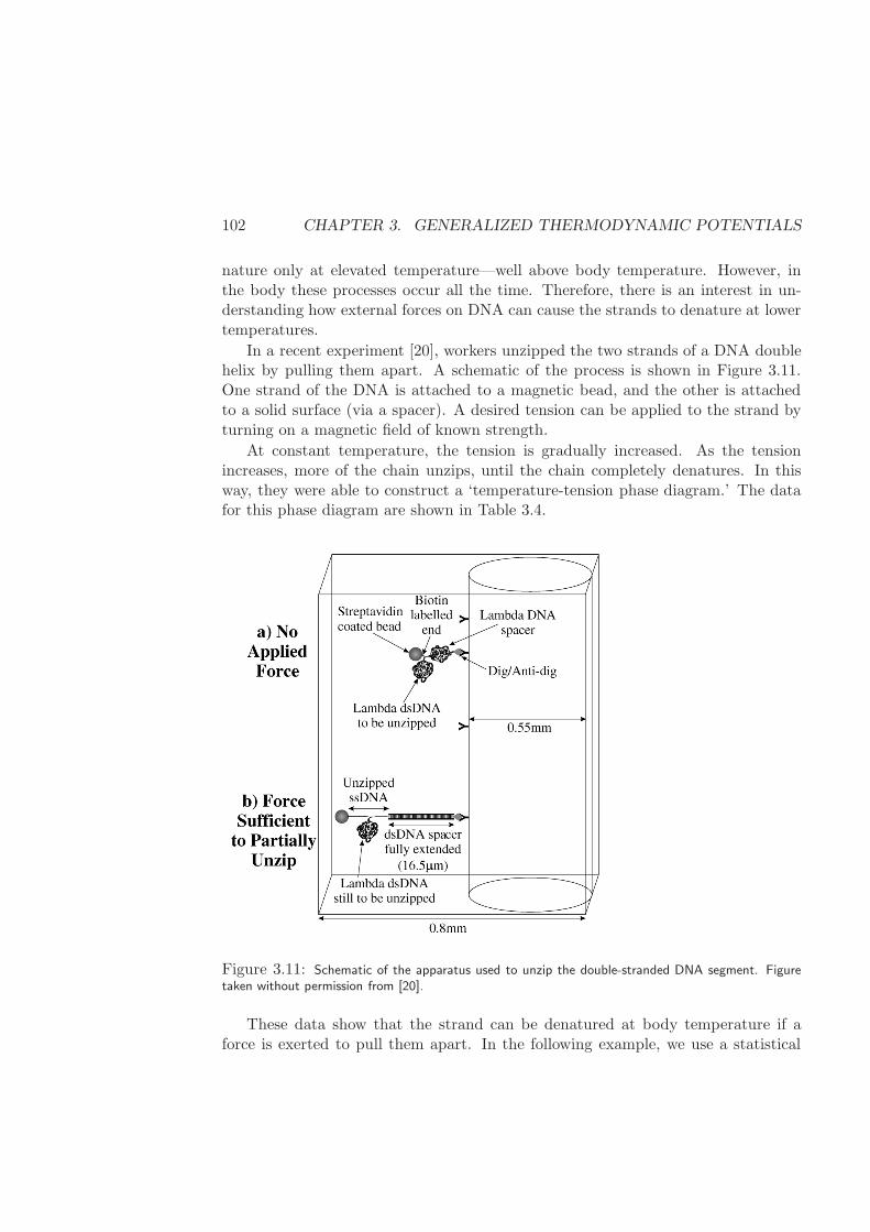
102 CHAPTER 3. GENERALIZED THERMODYNAMIC POTENTIALS
nature only at elevated temperature—well above body temperature. However, inthe body these processes occur all the time. Therefore, there is an interest in un-derstanding how external forces on DNA can cause the strands to denature at lowertemperatures.
In a recent experiment [20], workers unzipped the two strands of a DNA doublehelix by pulling them apart. A schematic of the process is shown in Figure 3.11.One strand of the DNA is attached to a magnetic bead, and the other is attachedto a solid surface (via a spacer). A desired tension can be applied to the strand byturning on a magnetic field of known strength.
At constant temperature, the tension is gradually increased. As the tensionincreases, more of the chain unzips, until the chain completely denatures. In thisway, they were able to construct a ‘temperature-tension phase diagram.’ The datafor this phase diagram are shown in Table 3.4.
Figure 3.11: Schematic of the apparatus used to unzip the double-stranded DNA segment. Figuretaken without permission from [20].
These data show that the strand can be denatured at body temperature if aforce is exerted to pull them apart. In the following example, we use a statistical
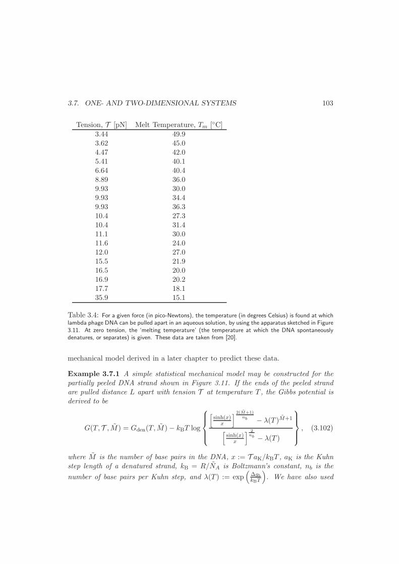
3.7. ONE- AND TWO-DIMENSIONAL SYSTEMS 103
Tension, T [pN] Melt Temperature, Tm [C]3.44 49.93.62 45.04.47 42.05.41 40.16.64 40.48.89 36.09.93 30.09.93 34.49.93 36.310.4 27.310.4 31.411.1 30.011.6 24.012.0 27.015.5 21.916.5 20.016.9 20.217.7 18.135.9 15.1
Table 3.4: For a given force (in pico-Newtons), the temperature (in degrees Celsius) is found at whichlambda phage DNA can be pulled apart in an aqueous solution, by using the apparatus sketched in Figure3.11. At zero tension, the ‘melting temperature’ (the temperature at which the DNA spontaneouslydenatures, or separates) is given. These data are taken from [20].
mechanical model derived in a later chapter to predict these data.
Example 3.7.1 A simple statistical mechanical model may be constructed for thepartially peeled DNA strand shown in Figure 3.11. If the ends of the peeled strandare pulled distance L apart with tension T at temperature T , the Gibbs potential isderived to be
G(T,T , M ) = Gden(T, M )− kBT log
[sinh(x)x
] 2(M+1)nb − λ(T )M+1
[sinh(x)x
] 2nb − λ(T )
, (3.102)
where M is the number of base pairs in the DNA, x := T aK/kBT , aK is the Kuhnstep length of a denatured strand, kB = R/NA is Boltzmann’s constant, nb is the
number of base pairs per Kuhn step, and λ(T ) := exp(
∆gbkBT
)
. We have also used
104 CHAPTER 3. GENERALIZED THERMODYNAMIC POTENTIALS
the difference in Gibbs potential between a single attached and unattached base pair∆gb(T ) := gu − ga. Eqn. (3.102) assumes that the free end of the coiled chain hasthe two strand ends covalently bonded. Therefore, when all of the base pairs aredetached, it is assumed that the DNA is one long single strand of 2M/nb Kuhnsteps. The real DNA strand has no such covalent bonding at its ends, of course.Hence, the model predicts complete peeling when all the base pairs are detached, andone long strand is made.
Using the above fundamental relation, find the distance L between the two ends ofthe unpeeled strands as a function of tension and temperature. For a given temper-ature, at a critical tension, this separation goes to infinity, which is the sought-after‘temperature-tension phase diagram’. Compare your result with the experimentalresults given in Table 3.4. Assume that ∆gb(T ) = ∆hb−T∆sb, where ∆hb and ∆sbare temperature independent. Assume that aK = 15A, nb = 5 (These estimates arefrom [92]). What values of ∆sb and ∆hb give the best fit? How does your estimateof ∆sb compare with the reported value (estimated using a different method, andin a different solvent) of ∆sb = 85J/K.mol? What do you predict for the meltingtemperature at zero tension?
Solution: Note that the fundamental relation given here is in terms of Kuhnsteps of size aK, whereas Exercise 2.9.E used the persistence length lp. Thepersistence length is equal to half the Kuhn step length, aK = 2lp. The contourlength of the two models should remain the same, so Np = 2NK.
First we find the separation length L as a function of (T, T , M). Recall thedifferential for the Gibbs potential, dG = −SdT + V dP + µdN , which, for the1D case becomes dG = −SdT − LdT + µdM . Hence, we find the length from
L = −(∂G
∂T
)
T,M
= −(∂x
∂T
)
T
(∂G
∂x
)
T,M
=
[
coth(x)− 1
x
]2aKnb
[
M + 1
1− λ(T, T )M+1− 1
1− λ(T, T )
]
, (3.103)
where we have introduced
λ(T, T ) := λ(T )
[x
sinh(x)
]2/nb
= exp
(∆gbkBT
)[ T aK/kBTsinh(T aK/kBT )
]2/nb
. (3.104)
We used the chain rule to obtain the second line of Eqn. (3.103), and we skippeda step of slightly messy algebra to obtain the last line.
3.7. ONE- AND TWO-DIMENSIONAL SYSTEMS 105
Eqn. (3.103) gives the average distance between the two free strand ends ata given tension, and a given temperature. This length has two coupled contri-butions, however: the tension pulls the detached segment of strands straight,and the temperature and tension detach additional base pairs. To find the rel-ative magnitude of these contributions, we can completely detach all the basepairs theoretically by letting the free energy of attachment become large andnegative: ∆gb → −∞. In that case, λ = 0, and the length becomes
LIL =
[
coth(x)− 1
x
]2MaKnb
. (3.105)
This is the length the chain would have for a given tension if all the base pairswere detached, and is called the Inverse Langevin force law [see Exercise3.7.B]. If we take the ratio of the two lengths, we obtain the expression
L
LIL=
[
1 + 1/M
1− λ(T, T )M+1− 1/M
1− λ(T, T )
]
, (3.106)
This ratio now includes only the effect of detaching base pairs. When it goesto 1, all the base pairs must be detached. We can make a plot of this ratioas a function of λ, as shown in Figure 3.12 for M = 1000. From this figurewe see that the chain “melts” when λ approaches 1. The value never becomesexactly 1, except for very small λ, which means very negative values for ∆gb,or large tensions. However, whenever λ is near one, it becomes very easy forthe number of attached base pairs to fluctuate to zero, at which point the twostrands will be irreversibly separated. It makes sense, then, to assume that thechain becomes completely unpeeled when λ ∼= 1.
Hence, the ‘modified melting temperature’ Tm = Tm(T ), is determined by
setting λ(Tm, T ) = 1. Or, taking the logarithm of each side, we can write
− ∆hbkBTm
+∆sbkB
=2
nblog
[ T aK/kBTmsinh(T aK/kBTm)
]
, (3.107)
where we replace the change in Gibbs potential per base pair upon melting,with the corresponding change in enthalpy and entropy, ∆gb = ∆hb−T∆sb. Ifwe neglect the temperature dependence of these two quantities, then we havefour parameters ∆hb, ∆sb, nb, and aK, three of which are already estimated
from other experiments. To fit the remaining parameter, we plot log[
xsinh(x)
]
vs. 1/Tm. For this plot it is useful to convert Boltzmann’s constant
kB = (1.38066× 10⁻²³J/K)(1N·m/J)(1012pN/N)(1010A/m)
= 0.138066 pN·A/K. (3.108)
Figure 3.13 shows the fit of our equation to the data (excluding the last point).The slope and intercept of the line are, then, −nb∆hb/(2kB) ∼= −11, 600± 900K, and nb∆sb/(2kB) ∼= 36± 3, respectively. Or, ∆hb ∼= 6.4× 10⁻²⁰J and ∆sb ∼=

106 CHAPTER 3. GENERALIZED THERMODYNAMIC POTENTIALS
λ
LL
IL
1.41.210.80.6
1
0.9
0.8
0.7
0.6
0.5
0.4
0.3
0.2
0.1
0
Figure 3.12: The end-to-end distance of a partially unzipped DNA strand as a function of the tension-modified base-pair partition function, λ. The distance is made dimensionless by the length the chainwould have if it were completely unzipped and there are M = 1000 base pairs. See Eqn. (3.106).
2.0×10⁻²²J/K. This latter value compares favorably with other estimates. Themelting temperature at zero tension is, according to Eqn. (3.107), Tm(T = 0) =∆hb/∆sb ∼= 320K, which is too low.
The last data point in the table does not fit well with the others. This pointmay not fit because (1) fluctuations are not accounted for in thermodynamics,and a large fluctuation at high tensions could lead to irreversible peeling8, (2)the free energy per base pair may be temperature dependent, (3) the model istoo simple, in that it does not account for so-called stacking of the adjacentnucleotides, or (4) there may be experimental error at that high tension. 2
3.7.3 Langmuir Adsorption
Here we consider a solid surface that has Ms moles of sites available for bindingN ≤ Ms moles of species A. Species A exists in an ideal gas phase above the solidsurface, but the molecules may attach to these adsorption sites, detach, or hopbetween adjacent sites on the surface. See Figure 3.14. Such a system is importantin catalysis, and some separation processes called pressure-swing adsorption (PSA).Adsorption measurements are also commonly used to calculate available surface area(See Problem 3.7.D).
Pressure-swing adsorption is used to separate oxygen from air for asthma pa-tients, methane from waste decomposition to produce fuel, and to remove moisture
8Fluctuations are covered in §6.7.
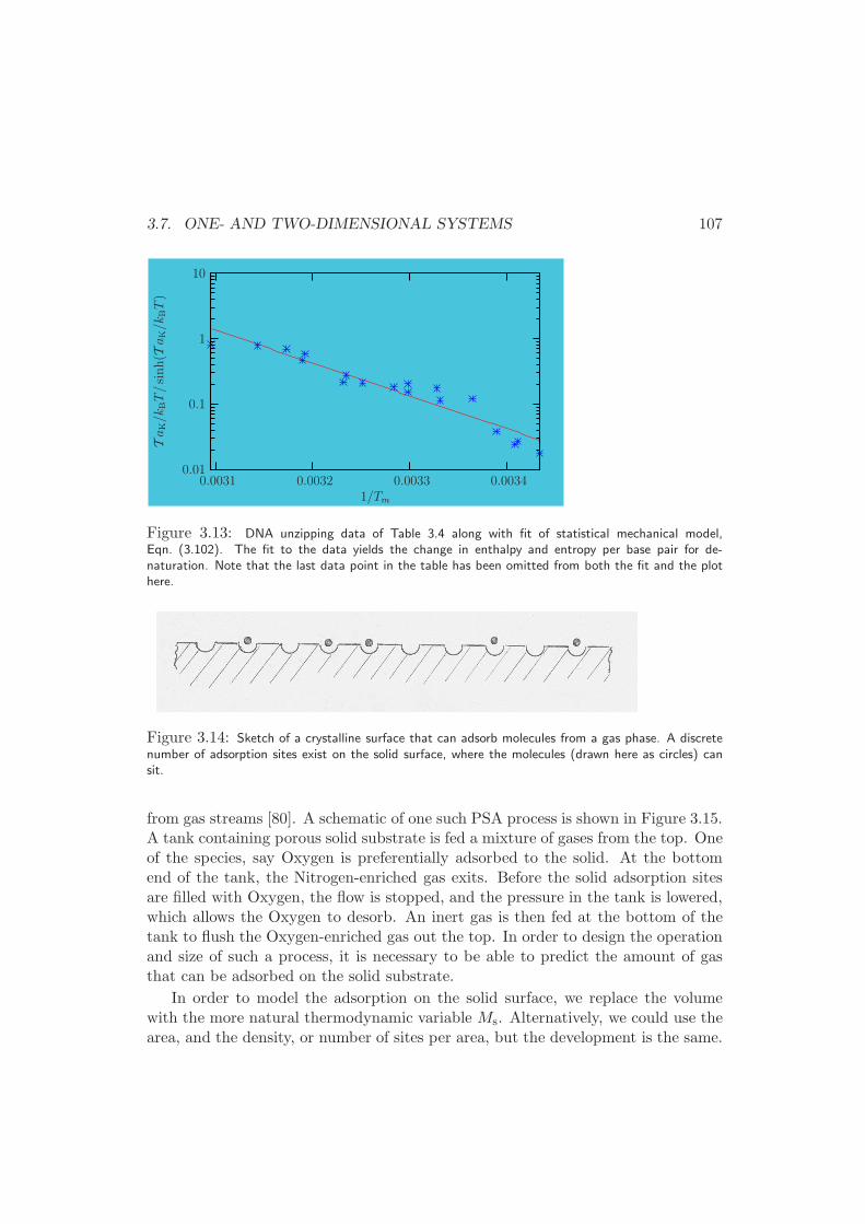
3.7. ONE- AND TWO-DIMENSIONAL SYSTEMS 107
1/Tm
Ta
K/k
BT
/si
nh(T
aK/k
BT
)
0.0031 0.0032 0.0033 0.0034
10
1
0.1
0.01
Figure 3.13: DNA unzipping data of Table 3.4 along with fit of statistical mechanical model,Eqn. (3.102). The fit to the data yields the change in enthalpy and entropy per base pair for de-naturation. Note that the last data point in the table has been omitted from both the fit and the plothere.
Figure 3.14: Sketch of a crystalline surface that can adsorb molecules from a gas phase. A discretenumber of adsorption sites exist on the solid surface, where the molecules (drawn here as circles) cansit.
from gas streams [80]. A schematic of one such PSA process is shown in Figure 3.15.A tank containing porous solid substrate is fed a mixture of gases from the top. Oneof the species, say Oxygen is preferentially adsorbed to the solid. At the bottomend of the tank, the Nitrogen-enriched gas exits. Before the solid adsorption sitesare filled with Oxygen, the flow is stopped, and the pressure in the tank is lowered,which allows the Oxygen to desorb. An inert gas is then fed at the bottom of thetank to flush the Oxygen-enriched gas out the top. In order to design the operationand size of such a process, it is necessary to be able to predict the amount of gasthat can be adsorbed on the solid substrate.
In order to model the adsorption on the solid surface, we replace the volumewith the more natural thermodynamic variable Ms. Alternatively, we could use thearea, and the density, or number of sites per area, but the development is the same.
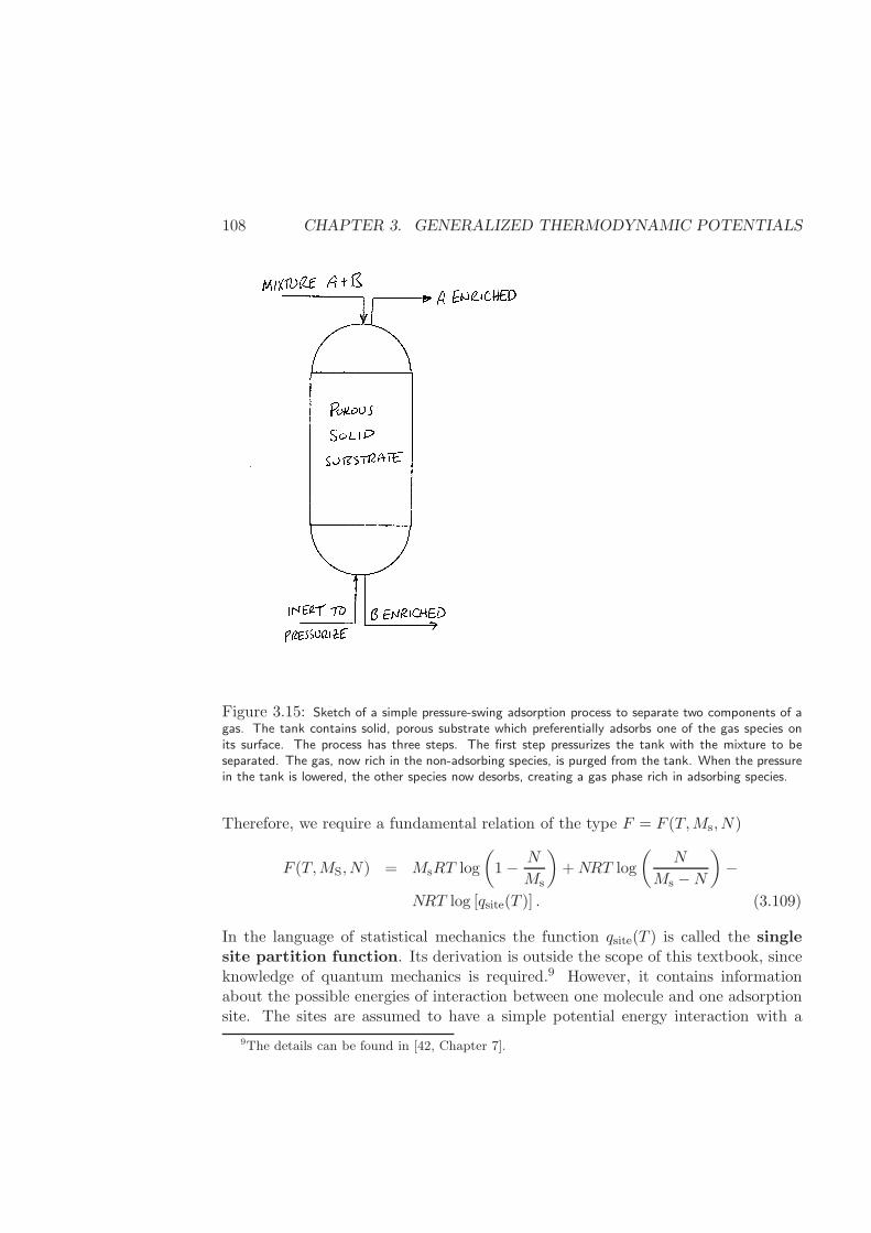
108 CHAPTER 3. GENERALIZED THERMODYNAMIC POTENTIALS
Figure 3.15: Sketch of a simple pressure-swing adsorption process to separate two components of agas. The tank contains solid, porous substrate which preferentially adsorbs one of the gas species onits surface. The process has three steps. The first step pressurizes the tank with the mixture to beseparated. The gas, now rich in the non-adsorbing species, is purged from the tank. When the pressurein the tank is lowered, the other species now desorbs, creating a gas phase rich in adsorbing species.
Therefore, we require a fundamental relation of the type F = F (T,Ms, N)
F (T,MS, N) = MsRT log
(
1− N
Ms
)
+NRT log
(N
Ms −N
)
−
NRT log [qsite(T )] . (3.109)
In the language of statistical mechanics the function qsite(T ) is called the singlesite partition function. Its derivation is outside the scope of this textbook, sinceknowledge of quantum mechanics is required.9 However, it contains informationabout the possible energies of interaction between one molecule and one adsorptionsite. The sites are assumed to have a simple potential energy interaction with a
9The details can be found in [42, Chapter 7].
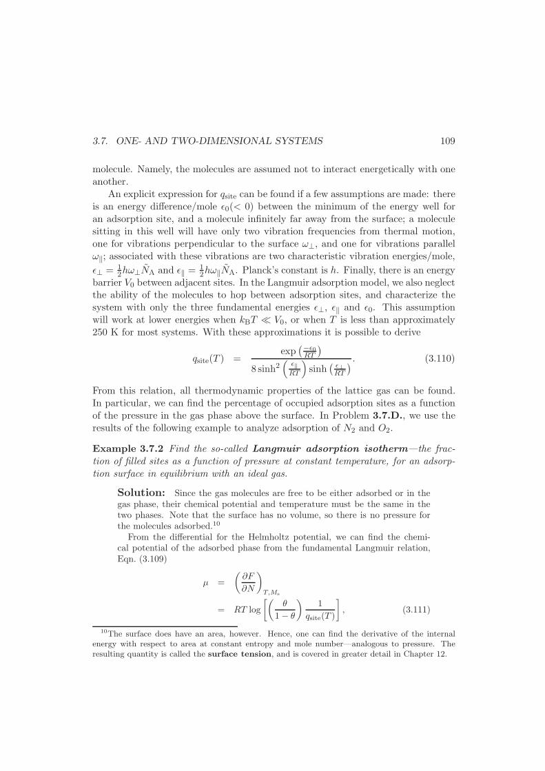
3.7. ONE- AND TWO-DIMENSIONAL SYSTEMS 109
molecule. Namely, the molecules are assumed not to interact energetically with oneanother.
An explicit expression for qsite can be found if a few assumptions are made: thereis an energy difference/mole ǫ0(< 0) between the minimum of the energy well foran adsorption site, and a molecule infinitely far away from the surface; a moleculesitting in this well will have only two vibration frequencies from thermal motion,one for vibrations perpendicular to the surface ω⊥, and one for vibrations parallelω‖; associated with these vibrations are two characteristic vibration energies/mole,
ǫ⊥ = 12hω⊥NA and ǫ‖ =
12hω‖NA. Planck’s constant is h. Finally, there is an energy
barrier V0 between adjacent sites. In the Langmuir adsorption model, we also neglectthe ability of the molecules to hop between adsorption sites, and characterize thesystem with only the three fundamental energies ǫ⊥, ǫ‖ and ǫ0. This assumptionwill work at lower energies when kBT ≪ V0, or when T is less than approximately250 K for most systems. With these approximations it is possible to derive
qsite(T ) =exp
(−ǫ0RT
)
8 sinh2(ǫ‖RT
)
sinh(ǫ⊥RT
) . (3.110)
From this relation, all thermodynamic properties of the lattice gas can be found.In particular, we can find the percentage of occupied adsorption sites as a functionof the pressure in the gas phase above the surface. In Problem 3.7.D., we use theresults of the following example to analyze adsorption of N2 and O2.
Example 3.7.2 Find the so-called Langmuir adsorption isotherm—the frac-tion of filled sites as a function of pressure at constant temperature, for an adsorp-tion surface in equilibrium with an ideal gas.
Solution: Since the gas molecules are free to be either adsorbed or in thegas phase, their chemical potential and temperature must be the same in thetwo phases. Note that the surface has no volume, so there is no pressure forthe molecules adsorbed.10
From the differential for the Helmholtz potential, we can find the chemi-cal potential of the adsorbed phase from the fundamental Langmuir relation,Eqn. (3.109)
µ =
(∂F
∂N
)
T,Ms
= RT log
[(θ
1− θ
)1
qsite(T )
]
, (3.111)
10The surface does have an area, however. Hence, one can find the derivative of the internalenergy with respect to area at constant entropy and mole number—analogous to pressure. Theresulting quantity is called the surface tension, and is covered in greater detail in Chapter 12.
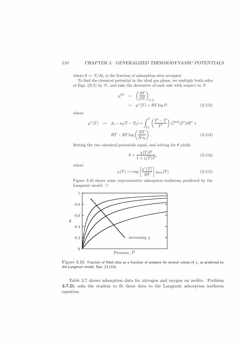
110 CHAPTER 3. GENERALIZED THERMODYNAMIC POTENTIALS
where θ := N/Ms is the fraction of adsorption sites occupied.To find the chemical potential in the ideal gas phase, we multiply both sides
of Eqn. (B.2) by N , and take the derivative of each side with respect to N
µIG =
(∂F
∂N
)
T,V
= µ(T ) +RT logP, (3.112)
where
µ(T ) := f0 − s0(T − T0) +
∫ T
T0
(T ′ − T
T ′
)
cidealv (T ′)dT ′ +
RT −RT log
(RT
Nv0
)
. (3.113)
Setting the two chemical potentials equal, and solving for θ yields
θ =χ(T )P
1 + χ(T )P, (3.114)
where
χ(T ) := exp
[µ(T )
RT
]
qsite(T ) (3.115)
Figure 3.16 shows some representative adsorption isotherms predicted by theLangmuir model. 2
0
0.2
0.4
0.6
0.8
1
θ
Pressure, P
increasing χ
I
Figure 3.16: Fraction of filled sites as a function of pressure for several values of χ, as predicted bythe Langmuir model, Eqn. (3.114).
Table 3.7 shows adsorption data for nitrogen and oxygen on zeolite. Problem3.7.D. asks the student to fit these data to the Langmuir adsorption isothermequation.
3.7. ONE- AND TWO-DIMENSIONAL SYSTEMS 111
The simple statistical mechanical model used to derive the Langmuir adsorptionmodel (given in §6.4) does not require that the adsorption sites be on a solid surface.Primarily, it assumes that adsorption sites do not interact energetically with oneanother. Hence, the result is much more general than just molecules adsorbingon solid surfaces. In fact, the equation is often used to model other adsorptionphenomenon, such as ligands adsorbing to proteins, or polymer chains to colloidalparticles. These examples are considered in the exercises.
In the following example, we use the Langmuir model to describe the bindingof proteins to sites on DNA. However, an additional subtlety must be taken intoaccount. For classical Langmuir adsorption, the chemical potential in the gas phaseis not affected by the degree of adsorption θ. However, in solution, every moleculeadsorbed decreases the concentration of unadsorbed molecules.
Example 3.7.3 Proteins bind to specific sites of DNA. It is believed that the pres-ence of other species can affect this adsorption, and we wish to examine that effecthere. Recently Heyduk and Lee [40] synthesized a 32-base-pair-long fragment ofDNA, which they tagged with a fluorescent dye. The dye makes it possible to mea-sure optically the fraction of DNA fragments that are bound by a specific protein. Wewon’t be concerned here with how this measurement works, but rather just assumethat it does.
Table 3.5 shows optical data for solutions of the E. Coli cyclic AMP receptorprotein (total concentration cTr ) and a 32-base-pair fragment DNA ligand of to-tal concentration cTD = 0.0111µM. Also present is cyclic adenosine monophosphate(cAMP), in two different concentrations, which is believed to play a role in binding,by forming complexes with the protein. We wish to study this role by using the Lang-muir model, and seeing how the binding parameter χ is affected by the concentrationof cAMP.
The anisotropy A is fluorescence data giving a measure of the amount of binding,and is assumed to be linearly proportional to the concentration of bound complex cB,and unbound DNA fragment cD
A = ADcD +ABcB, (3.116)
where AD and AB are the (constant) anisotropies of the free and bound DNA, re-spectively. Use the data in the table to estimate the binding parameter χ for eachconcentration of ligand. Does its value depend upon cAMP concentration? Cananything be inferred about the presence of cAMP on DNA/protein binding?
Solution: Assuming constant volume, we note that the total concentrationof protein cTr is constant, and the sum of free protein cr and bound protein
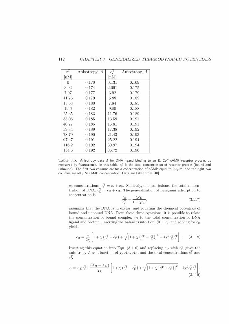
112 CHAPTER 3. GENERALIZED THERMODYNAMIC POTENTIALS
cTr Anisotropy, A cTr Anisotropy, A[nM] [nM]
0 0.170 0.131 0.1693.92 0.174 2.091 0.1757.97 0.177 3.92 0.17911.76 0.179 5.88 0.18215.68 0.180 7.84 0.18519.6 0.182 9.80 0.18825.35 0.183 11.76 0.18933.06 0.185 13.59 0.19140.77 0.185 15.81 0.19159.84 0.189 17.38 0.19278.79 0.190 21.43 0.19397.47 0.191 25.22 0.194116.2 0.192 30.97 0.194134.6 0.192 36.72 0.196
Table 3.5: Anisotropy data A for DNA ligand binding to an E. Coli cAMP receptor protein, asmeasured by fluorescence. In this table, cTr is the total concentration of receptor protein (bound andunbound). The first two columns are for a concentration of cAMP equal to 0.5µM, and the right twocolumns are 500µM cAMP concentration. Data are taken from [40].
cB concentrations: cTr = cr + cB. Similarly, one can balance the total concen-tration of DNA, cTD = cD + cB. The generalization of Langmuir adsorption toconcentration is
cBcTr
=χcD
1 + χcD, (3.117)
assuming that the DNA is in excess, and equating the chemical potentials ofbound and unbound DNA. From these three equations, it is possible to relatethe concentration of bound complex cB to the total concentration of DNAligand and protein. Inserting the balances into Eqn. (3.117), and solving for cByields
cB =1
2χ
[
1 + χ(cTr + cTD
)+
√[1 + χ
(cTr + cTD
)]2 − 4χ2cTDcTr
]
, (3.118)
Inserting this equation into Eqn. (3.116) and replacing cD with cTD gives theanisotropy A as a function of χ, AD, AB, and the total concentrations cTr andcTD.
A = ADcTD+
(AB −AD)
2χ
[
1 + χ(cTr + cTD
)+
√[1 + χ
(cTr + cTD
)]2 − 4χ2cTDcTr
]
.
(3.119)
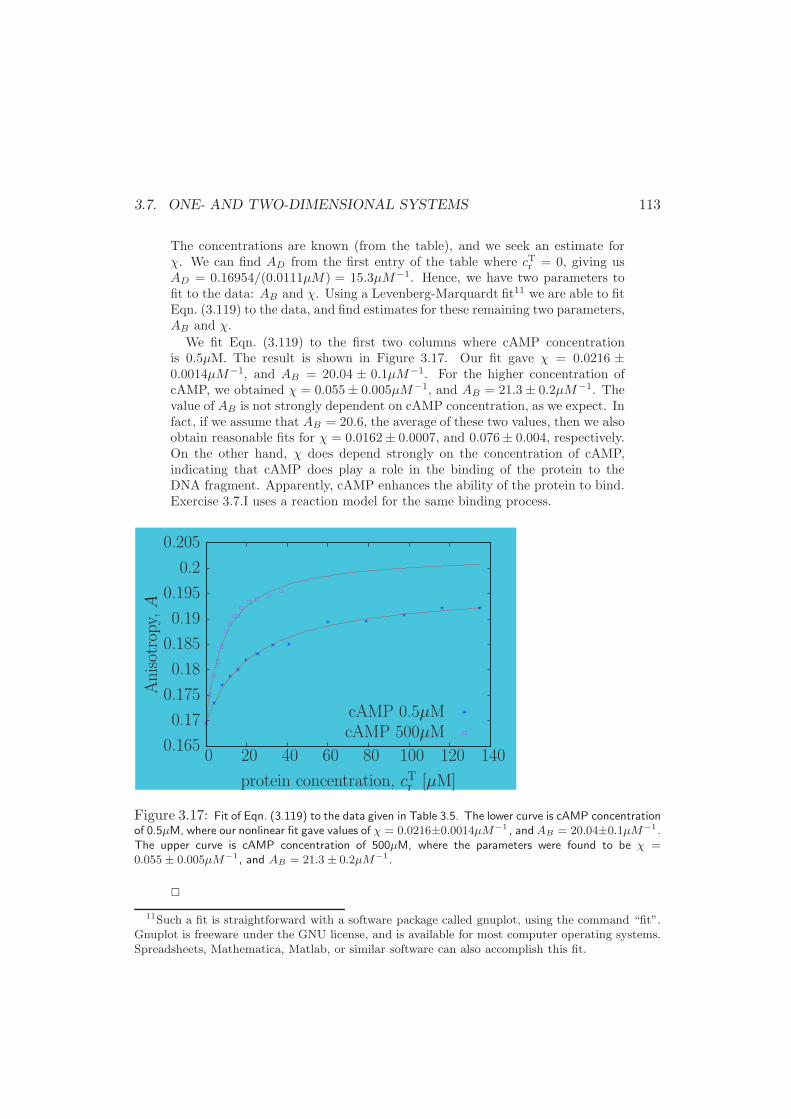
3.7. ONE- AND TWO-DIMENSIONAL SYSTEMS 113
The concentrations are known (from the table), and we seek an estimate forχ. We can find AD from the first entry of the table where cTr = 0, giving usAD = 0.16954/(0.0111µM) = 15.3µM−1. Hence, we have two parameters tofit to the data: AB and χ. Using a Levenberg-Marquardt fit11 we are able to fitEqn. (3.119) to the data, and find estimates for these remaining two parameters,AB and χ.
We fit Eqn. (3.119) to the first two columns where cAMP concentrationis 0.5µM. The result is shown in Figure 3.17. Our fit gave χ = 0.0216 ±0.0014µM−1, and AB = 20.04 ± 0.1µM−1. For the higher concentration ofcAMP, we obtained χ = 0.055± 0.005µM−1, and AB = 21.3± 0.2µM−1. Thevalue of AB is not strongly dependent on cAMP concentration, as we expect. Infact, if we assume that AB = 20.6, the average of these two values, then we alsoobtain reasonable fits for χ = 0.0162± 0.0007, and 0.076± 0.004, respectively.On the other hand, χ does depend strongly on the concentration of cAMP,indicating that cAMP does play a role in the binding of the protein to theDNA fragment. Apparently, cAMP enhances the ability of the protein to bind.Exercise 3.7.I uses a reaction model for the same binding process.
cAMP 500µMcAMP 0.5µM
protein concentration, cTr [µM]
Anis
otro
py,A
140120100806040200
0.205
0.2
0.195
0.19
0.185
0.18
0.175
0.17
0.165
Figure 3.17: Fit of Eqn. (3.119) to the data given in Table 3.5. The lower curve is cAMP concentrationof 0.5µM, where our nonlinear fit gave values of χ = 0.0216±0.0014µM−1 , andAB = 20.04±0.1µM−1 .The upper curve is cAMP concentration of 500µM, where the parameters were found to be χ =0.055 ± 0.005µM−1 , and AB = 21.3 ± 0.2µM−1 .
2
11Such a fit is straightforward with a software package called gnuplot, using the command “fit”.Gnuplot is freeware under the GNU license, and is available for most computer operating systems.Spreadsheets, Mathematica, Matlab, or similar software can also accomplish this fit.
114 CHAPTER 3. GENERALIZED THERMODYNAMIC POTENTIALS
3.8 Summary
In the previous chapter, we covered internal energy U , entropy S, temperature T ,pressure P , chemical potential µi, heat flow Q, work W , and the five postulates ofthermodynamics. We proved that these postulates and definitions fit our intuitionabout temperature and heat flow, pressure and expansion, and about mass flow.
In this chapter, we used Legendre Transforms to define new thermodynamicquantities with complete thermodynamic information:
• Enthalpy H := U + PV , (3.9)
• Helmholtz potential F := U − TS, (3.10)
• Gibbs free energy G := U − TS + PV , (3.11)
We proved that an isolated system at equilibrium has minimum internal energyat constant entropy, volume and mole number. The other subsystems are summa-rized in Table 3.2.
Each of the generalized potentials has a canonical differential, which can be usedto derive equations of state, or Maxwell relations. These differentials are
dU = TdS − PdV +∑
i
µidNi, (3.48)
dH = TdS + V dP +∑
i
µidNi, (3.49)
dF = −SdT − PdV +∑
i
µidNi, (3.50)
dG = −SdT + V dP +∑
i
µidNi. (3.51)
The Maxwell relations are derived from these differentials by using the analyticproperty of the potentials, Eqn. (A.5). The differentials, and the Maxwell relationsare conveniently memorized through the thermodynamic square, Figure 3.5.
These are not the only such generalized potentials, but are the most common.For example, in Problem 3.3.D. we introduce another such potential common instatistical mechanics.
Along the way, we derived the Euler Relation
U = TS − PV +r∑
i=1
µiNi, Euler Relation, (3.20)

3.8. SUMMARY 115
and the Gibbs-Duhem Relation
0 = SdT − V dP +
m∑
i=1
Nidµi, Gibbs-Duhem Relation. (3.22)
The Euler relation shows that the specific Gibbs potential is identical to the chemicalpotential for pure substances. The Gibbs-Duhem relation is useful for mixtures,considered later in this book.
We also proved that the generalized potentials are useful for calculating work inisothermal and/or isobaric conditions.
We defined three (of many possible) second-order derivatives
• The coefficient of thermal expansion α := 1v
(∂v∂T
)
P.
• The isothermal compressibility κT := − 1v
(∂v∂P
)
T.
• The constant-pressure heat capacity cP := T(∂s∂T
)
P.
All other second-order derivatives can be found in relation to these, for a single-component system. In fact, any thermodynamic quantity for a single-componentsystem can be found from these quantities (§3.6).
Complete thermodynamic information for a pure substance is also contained intwo equations of state (e.g., P = P (T, v), u = u(T, v)), or in three relations forsecond-order derivatives (e.g., α = α(T, P ), κT = κT (T, P ), cP = cP (T, P )).
As example models, we considered the general ideal gas, Eqn. (3.16), and anonlinear elastic strand, Eqn. (3.100).
We also analyzed the following problems
• Adiabatic and isothermal compression of ammonia, Example 3.2.2.
• A heat engine, Example 3.2.3.
• A fuel cell, Example 3.5.4.
• Deriving a fundamental relation for a non-ideal, elastic strand, §3.7.1.
• Unzipping a single strand of DNA by using tension and heat, Example 3.7.1.
• Langmuir adsorption on a solid surface, Example 3.7.2.
• Binding of a protein to a DNA fragment, Example 3.7.3.
In §3.7.1, we showed how to generate a fundamental relation from two equationsof state for a general elastic string. We also predicted the fractional adsorptionof molecules on a solid surface as a function of pressure, the so-called “Langmuirisotherm.”
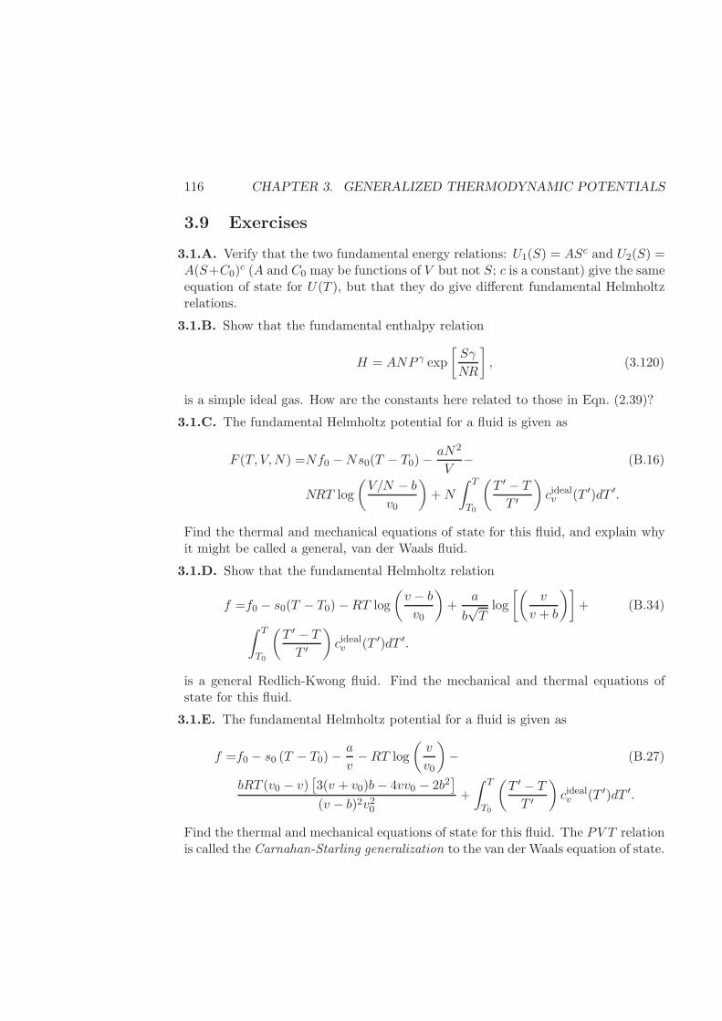
116 CHAPTER 3. GENERALIZED THERMODYNAMIC POTENTIALS
3.9 Exercises
3.1.A. Verify that the two fundamental energy relations: U1(S) = ASc and U2(S) =A(S+C0)
c (A and C0 may be functions of V but not S; c is a constant) give the sameequation of state for U(T ), but that they do give different fundamental Helmholtzrelations.
3.1.B. Show that the fundamental enthalpy relation
H = ANP γ exp
[Sγ
NR
]
, (3.120)
is a simple ideal gas. How are the constants here related to those in Eqn. (2.39)?
3.1.C. The fundamental Helmholtz potential for a fluid is given as
F (T, V,N) =Nf0 −Ns0(T − T0)−aN2
V− (B.16)
NRT log
(V/N − b
v0
)
+N
∫ T
T0
(T ′ − T
T ′
)
cidealv (T ′)dT ′.
Find the thermal and mechanical equations of state for this fluid, and explain whyit might be called a general, van der Waals fluid.
3.1.D. Show that the fundamental Helmholtz relation
f =f0 − s0(T − T0)−RT log
(v − b
v0
)
+a
b√T
log
[(v
v + b
)]
+ (B.34)
∫ T
T0
(T ′ − T
T ′
)
cidealv (T ′)dT ′.
is a general Redlich-Kwong fluid. Find the mechanical and thermal equations ofstate for this fluid.
3.1.E. The fundamental Helmholtz potential for a fluid is given as
f =f0 − s0 (T − T0)−a
v−RT log
(v
v0
)
− (B.27)
bRT (v0 − v)[3(v + v0)b− 4vv0 − 2b2
]
(v − b)2v20+
∫ T
T0
(T ′ − T
T ′
)
cidealv (T ′)dT ′.
Find the thermal and mechanical equations of state for this fluid. The PV T relationis called the Carnahan-Starling generalization to the van der Waals equation of state.
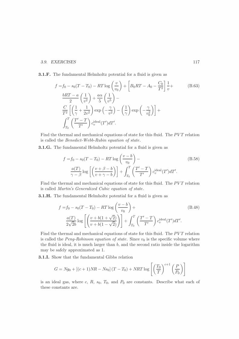
3.9. EXERCISES 117
3.1.F. The fundamental Helmholtz potential for a fluid is given as
f =f0 − s0(T − T0)−RT log
(v
v0
)
+
[
B0RT −A0 −C0
T 2
]1
v+ (B.63)
bRT − a
2
(1
v2
)
+aα
5
(1
v5
)
−
C
T 2
[(1
γ+
1
2v2
)
exp(
− γ
v2
)
−(1
γ
)
exp
(
− γ
v20
)]
+
∫ T
T0
(T ′ − T
T ′
)
cidealv (T ′)dT ′.
Find the thermal and mechanical equations of state for this fluid. The PV T relationis called the Benedict-Webb-Rubin equation of state.
3.1.G. The fundamental Helmholtz potential for a fluid is given as
f =f0 − s0(T − T0)−RT log
(v − b
v0
)
− (B.58)
a(T )
γ − βlog
[(v + β − b
v + γ − b
)]
+
∫ T
T0
(T ′ − T
T ′
)
cidealv (T ′)dT ′.
Find the thermal and mechanical equations of state for this fluid. The PV T relationis called Martin’s Generalized Cubic equation of state.
3.1.H. The fundamental Helmholtz potential for a fluid is given as
f =f0 − s0(T − T0)−RT log
(v − b
v0
)
+ (B.48)
a(T )
2√2b
log
[(
v + b(1 +√2)
v + b(1−√2)
)]
+
∫ T
T0
(T ′ − T
T ′
)
cidealv (T ′)dT ′.
Find the thermal and mechanical equations of state for this fluid. The PV T relationis called the Peng-Robinson equation of state. Since v0 is the specific volume wherethe fluid is ideal, it is much larger than b, and the second ratio inside the logarithmmay be safely approximated as 1.
3.1.I. Show that the fundamental Gibbs relation
G = Ng0 + [(c+ 1)NR−Ns0] (T − T0) +NRT log
[(T0T
)c+1( P
P0
)]
is an ideal gas, where c, R, s0, T0, and P0 are constants. Describe what each ofthese constants are.
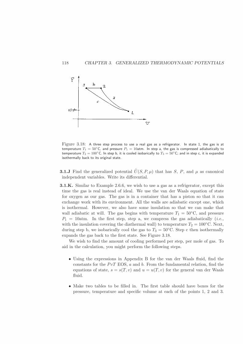
118 CHAPTER 3. GENERALIZED THERMODYNAMIC POTENTIALS
Figure 3.18: A three step process to use a real gas as a refrigerator. In state 1, the gas is attemperature T1 = 50C, and pressure P1 = 10atm. In step a, the gas is compressed adiabatically totemperature T2 = 100C. In step b, it is cooled isobarically to T3 = 50C; and in step c, it is expandedisothermally back to its original state.
3.1.J Find the generalized potential U(S,P, µ) that has S, P , and µ as canonicalindependent variables. Write its differential.
3.1.K. Similar to Example 2.6.6, we wish to use a gas as a refrigerator, except thistime the gas is real instead of ideal. We use the van der Waals equation of statefor oxygen as our gas. The gas is in a container that has a piston so that it canexchange work with its environment. All the walls are adiabatic except one, whichis isothermal. However, we also have some insulation so that we can make thatwall adiabatic at will. The gas begins with temperature T1 = 50C, and pressureP1 = 10atm. In the first step, step a, we compress the gas adiabatically (i.e.,with the insulation covering the diathermal wall) to temperature T2 = 100C. Next,during step b, we isobarically cool the gas to T3 = 50C. Step c then isothermallyexpands the gas back to the first state. See Figure 3.18.
We wish to find the amount of cooling performed per step, per mole of gas. Toaid in the calculation, you might perform the following steps.
• Using the expressions in Appendix B for the van der Waals fluid, find theconstants for the PvT EOS, a and b. From the fundamental relation, find theequations of state, s = s(T, v) and u = u(T, v) for the general van der Waalsfluid.
• Make two tables to be filled in. The first table should have boxes for thepressure, temperature and specific volume at each of the points 1, 2 and 3.
3.9. EXERCISES 119
The second table should have boxes for ∆u, Q and W for each of the steps a,b and c. Fill in the boxes from the problem statement.
• Now begin filling in each of the boxes from the necessary calculations. Forexample, you could use the PvT EOS to find the specific volume v1.
Then, step a is assumed adiabatic and reversible, so it is isentropic. Use yourentropy equation of state above to find the specific volume v2. From T2 andv2, you should be able to find the pressure P2. From your u EOS, you can alsofind the change in internal energy in step a, ∆ua. From an energy balance,you can find Qa.
• Continue filling out the tables in this way. When finished, calculate the totalwork necessary, and amount of cooling that can be accomplished. Which stepsrequire work, and which steps provide cooling?
As a bonus, you could also run the machine backwards and use heat to generatework. In that case, how much work is generated per amount of heat added to thesystem?
3.1.L. Use the thermodynamics diagram for ammonia on p.212 to estimate thechange in chemical potential for ammonia at constant T = 140C, but pressurechanging from 20 to 1MPa.
3.2.A. Prove that a system in contact with both a pressure and a temperaturereservoir reaches equilibrium when dGsys = 0.
3.2.B. Use the result of Example 3.2.1 to find the quasi-static work required tocompress one mole of oxygen isothermally at 170 K from 2 to 0.8 liter using aPeng-Robinson equation of state. Can you think of another way to find this result?
3.2.C. Using the results of Example 3.2.1, find the work necessary to compress re-versibly and isothermally one mole of ethane at 330K from 8 to 1 liters. Use theBenedict-Webb-Rubin equation of state.
3.2.D. Using the figure on p.212, find the work necessary to compress ammoniaisothermally from a density of 2kg/m3 to 250 kg/m3 at 340C.
3.2.E. Using the results of Example 3.2.1, find the work necessary to compress re-versibly and isothermally one mole of DuPont refrigerant HCFC-123 at 330K from200 to 105 liters. Apparently, this fluid is well described by a modified Benedict-Webb-Rubin equation of state. Details of the appropriate equation of state arefound at:
http://www.dupont.com/suva/na/usa/literature/pdf/h47753.pdf.This document also contains tables of thermodynamic properties, which may be
used to avoid explicit use of the equation of state altogether.
120 CHAPTER 3. GENERALIZED THERMODYNAMIC POTENTIALS
3.2.F. Using the figure on p.212, find the work necessary to compress 5 l of ammoniaadiabatically from a density of 2kg/m3 and pressure of 250 kPa to a density of 60kg/m3.
3.3.A. Derive the differentials for the generalized potentials H and G.
3.3.B. Derive the remaining Maxwell relations, Eqs. (3.56), (3.58), and (3.59).
3.3.C. In Example 3.1.2, we found S(T, V ) in Eqn. (3.17) for a general ideal gas.Verify that the third Maxwell relation is satisfied for the general ideal gas. Verifythe other three relations.
3.3.D. In this chapter we performed a Legendre transform on the internal energy inthe variables S and V . One may also perform transforms in the variable N , or onthe entropy. By performing a Legendre transform on U in the mole number, findthe definition of the generalized potential Ψ with canonical independent variables(T, V, µ). Find the differential for this variable, and show that
(∂Ψ
∂µ
)
T,V
= −N. (3.121)
This generalized potential frequently arises in statistical mechanics, but is often thenegative of the one defined here.
3.3.E. Prove the Maxwell-like relation(∂µi∂P
)
T,Nj=
(∂V
∂Ni
)
T,P,Nj 6=i(3.122)
3.3.F. A methanol fuel cell relies on the reaction
CH3OH +3
2O2 → CO2 + 2H2O.
Find the maximum available work as a function of temperature for this fuel cell,assuming that it works reversibly. Also find the maximum work available from aheat engine. Do your results agree with Table 3.3?
3.5.A. Find the coefficient of thermal expansion and the heat capacity for the simplevan der Waals fluid.
3.5.B. Find the isothermal compressibility and heat capacity predicted by the Redlich-Kwong equation of state in §B.5.3.5.C. Find the isothermal compressibility and heat capacity predicted by the Peng-Robinson equation of state in §B.6.
3.9. EXERCISES 121
3.5.D. It is reported that the isothermal compressibility at the boiling point (whichis reported as -252.77C) for hydrogen is -50.3MPa−1 . How does this value comparewith the prediction by the van der Waals equation of state? Note that the constantsfor the van der Waals fluid may be found from critical data by Eqn. (4.22).
3.5.E. Find α as predicted by the Peng-Robinson Equation of State.
3.5.F. Find α as predicted by the Redlich-Kwong model.
3.5.G. Use the Soave-Redlich-Kwong model (§B.5) to estimate the constant-pressureheat capacity of water at 25C and 2bar.
3.5.H. Using the Peng-Robinson model, derive an expression for the constant-volume
heat capacity. Make a plot of cv−cidealv
cidealvfor pure nitrogen as a function of pressure
at room temperature. Your pressure range should be 1 to 100 atmospheres. Theparameters for the Peng-Robinson model can be found from the critical point prop-erties using the equations given in the appendix.
3.6.A. What is the constant-volume heat capacity for a simple ideal gas?
3.6.B. What is(∂U∂T
)
Pfor a general ideal gas?
3.6.C. Reduce the following derivatives in terms of standard quantities.
(1)(∂S∂V
)
P; (2)
(∂V∂T
)
S; (3)
(∂H∂V
)
T; (4)
(∂V∂P
)
H; (5)
(∂V∂S
)
H
3.6.D. Find an expression that relates the isentropic compressibility κS to thethree second-order derivatives α, κT , and cP :
κS := −1
v
(∂v
∂P
)
S,N
. (3.123)
What is κS for a simple ideal gas?
3.6.E. Find the change in chemical potential for steam at 400C which is compressedfrom 0.5 to 2MPa. Explain why one cannot use the steam tables to find the changein chemical potential for steam undergoing temperature changes. Hint: look atthe entry for the entropy of saturated liquid at 0C. Does it agree with the Nernstpostulate? How could this problem be fixed, so that one could use the steam tables?
3.6.F. Express the Joule-Thomson coefficient
(∂T
∂P
)
H,N
, Joule-Thomson coefficient (3.124)
in terms of measurable quantities.
122 CHAPTER 3. GENERALIZED THERMODYNAMIC POTENTIALS
3.6.G. The Joule-Thompson coefficient defined in the previous problem is useful inflow through valves. As is shown in Chapter 5.2, if one assumes that flow across avalve is adiabatic, it is also isenthalpic. Hence, the change in temperature as thepressure drops across the valve can be found from the Joule-Thompson coefficient.Find the change in temperature when the pressure of ammonia drops from 200MPaand 180C, to a pressure of 50MPa in two ways: (1) using the thermodynamicdiagram on p.212, and (2) using the Peng-Robinson model.
3.6.H. 1. Find(∂T∂P
)
S,Nas a function of temperature and volume for a general
ideal gas.
2. Make a plot of(∂T∂P
)
S,Nfor oxygen at room temperature as a function of
pressure between 1 and 3 atm.
3. Integrate your expression from (1) to find an expression that relates tempera-ture to pressure. Note that the expression is not explicit in temperature (i.e.,it is not possible to write an equation of the form T = T (P )). However, itcan be made explicit in pressure: P = P (T ). Can you figure out a way toplot the temperature as a function of pressure during the reversible, adiabaticcompression of part (2)?
3.6.I. Using the result of Problem 3.5.G. and thermodynamic manipulations, findthe constant-pressure heat capacity of liquid water at the same temperature andpressure.
3.6.J. Find a relationship between the constant-tension heat capacity, and the constant-length heat capacity and other measurable quantities.
3.7.A. Find the mechanical and thermal equations of state for the rubber band withthe fundamental Helmholtz relation
F = f0L0 − s0L0(T − T0)−1
2NcRT log
[
1−(L− L0
L1 − L0
)2]
+
L0
∫ T
T0
(T ′ − T
T ′
)
cL(T′)dT ′. (3.125)
The quantities Nc, L0, and L1 are constants. cL is some known function of T .
3.7.B. Another statistical mechanical model for a single strand of DNA (see Prob-lem 2.9.E.) is called the inverse Langevin force law with Gibbs potential
G(T,T ) = g0L0 − (T − T0)s0L0 − L0
∫ T
T0
(T − T ′
T ′
)
c0T (T′)dT ′ −
NKkBT log
[kBT
T aKsinh
(T aKkBT
)]
, (3.126)
3.9. EXERCISES 123
where, as before, NK is the number of segments, aK is the length of a segment, kBis Boltzmann’s constant, and we have introduced the zero-tension heat capacity forthe chain C0
T (T′). How well does this model describe the data given in Table 2.1 on
page 60? Be sure to read the comments about persistence length versus Kuhn steplength in the solution to Example 3.7.1.
3.7.C. Here we derive a method to measure the contributions of entropy and internalenergy to the elasticity T . For isothermal stretching, we may write
T =
(∂F
∂L
)
T
=
(∂U
∂L
)
T
− T
(∂S
∂L
)
T
(3.127)
where the second line is obtained from the definition for F . We then seek a wayto estimate the contribution from each of the two terms on the right side of thisexpression.
First, derive a generalized Maxwell relation to relate (∂S/∂L)T to measurablequantities (T,L,T ). Then, use the generalized differential for U to obtain (∂U/∂L)Tin terms of measurables. By ‘generalized’, we mean here where we have replacedthe usual variables (S, V,N) with the new set appropriate for a rubber band (S,L).Finally, explain how measurements of tension at different values of T but fixed Lcan be used to estimate the contributions of entropy and internal energy to theelasticity at a given L.
Use the data in Table 3.6, which contains tension versus extension length datafor a cross-linked rubber, to make a plot of
(∂U∂L
)
Tand −T
(∂S∂L
)
T(divided by area)
versus (L− L0)/L0 for rubber. To a first approximation, you may assume that thevolume is constant during stretch, so that the area A = A0L0/L
2, where A0 is thecross-sectional area in the unstretched state.
3.7.D. Table 3.7 shows the amount of Oxygen and Nitrogen that adsorb to solidzeolite as a function of pressure at 293K. In order to design a pressure swing adsorber,it is necessary to find the Langmuir adsorption function χ(T ) at this temperaturefor each species. Using these data, find the maximum amount of each species thatcan be adsorbed per gram of zeolite ρmax, and χ(T = 293K). Find an estimate forthe size of an oxygen or nitrogen molecule, and use this size to approximate theamount of surface area per mass of zeolite.
3.7.E. The B.E.T.(Brunauer-Emmett-Teller) model for multilayer chemical adsorp-tion. If we generalize the statistical mechanical Langmuir model for adsorption toallow for more than one molecule to adsorb on a single site, we find the following
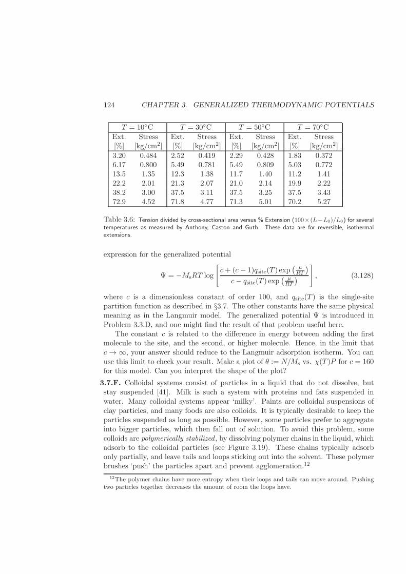
124 CHAPTER 3. GENERALIZED THERMODYNAMIC POTENTIALS
T = 10C T = 30C T = 50C T = 70CExt. Stress Ext. Stress Ext. Stress Ext. Stress[%] [kg/cm2] [%] [kg/cm2] [%] [kg/cm2] [%] [kg/cm2]
3.20 0.484 2.52 0.419 2.29 0.428 1.83 0.3726.17 0.800 5.49 0.781 5.49 0.809 5.03 0.77213.5 1.35 12.3 1.38 11.7 1.40 11.2 1.4122.2 2.01 21.3 2.07 21.0 2.14 19.9 2.2238.2 3.00 37.5 3.11 37.5 3.25 37.5 3.4372.9 4.52 71.8 4.77 71.3 5.01 70.2 5.27
Table 3.6: Tension divided by cross-sectional area versus % Extension (100× (L−L0)/L0) for severaltemperatures as measured by Anthony, Caston and Guth. These data are for reversible, isothermalextensions.
expression for the generalized potential
Ψ = −MsRT log
[
c+ (c− 1)qsite(T ) exp( µRT
)
c− qsite(T ) exp( µRT
)
]
, (3.128)
where c is a dimensionless constant of order 100, and qsite(T ) is the single-sitepartition function as described in §3.7. The other constants have the same physicalmeaning as in the Langmuir model. The generalized potential Ψ is introduced inProblem 3.3.D, and one might find the result of that problem useful here.
The constant c is related to the difference in energy between adding the firstmolecule to the site, and the second, or higher molecule. Hence, in the limit thatc → ∞, your answer should reduce to the Langmuir adsorption isotherm. You canuse this limit to check your result. Make a plot of θ := N/Ms vs. χ(T )P for c = 160for this model. Can you interpret the shape of the plot?
3.7.F. Colloidal systems consist of particles in a liquid that do not dissolve, butstay suspended [41]. Milk is such a system with proteins and fats suspended inwater. Many colloidal systems appear ‘milky’. Paints are colloidal suspensions ofclay particles, and many foods are also colloids. It is typically desirable to keep theparticles suspended as long as possible. However, some particles prefer to aggregateinto bigger particles, which then fall out of solution. To avoid this problem, somecolloids are polymerically stabilized , by dissolving polymer chains in the liquid, whichadsorb to the colloidal particles (see Figure 3.19). These chains typically adsorbonly partially, and leave tails and loops sticking out into the solvent. These polymerbrushes ‘push’ the particles apart and prevent agglomeration.12
12The polymer chains have more entropy when their loops and tails can move around. Pushingtwo particles together decreases the amount of room the loops have.
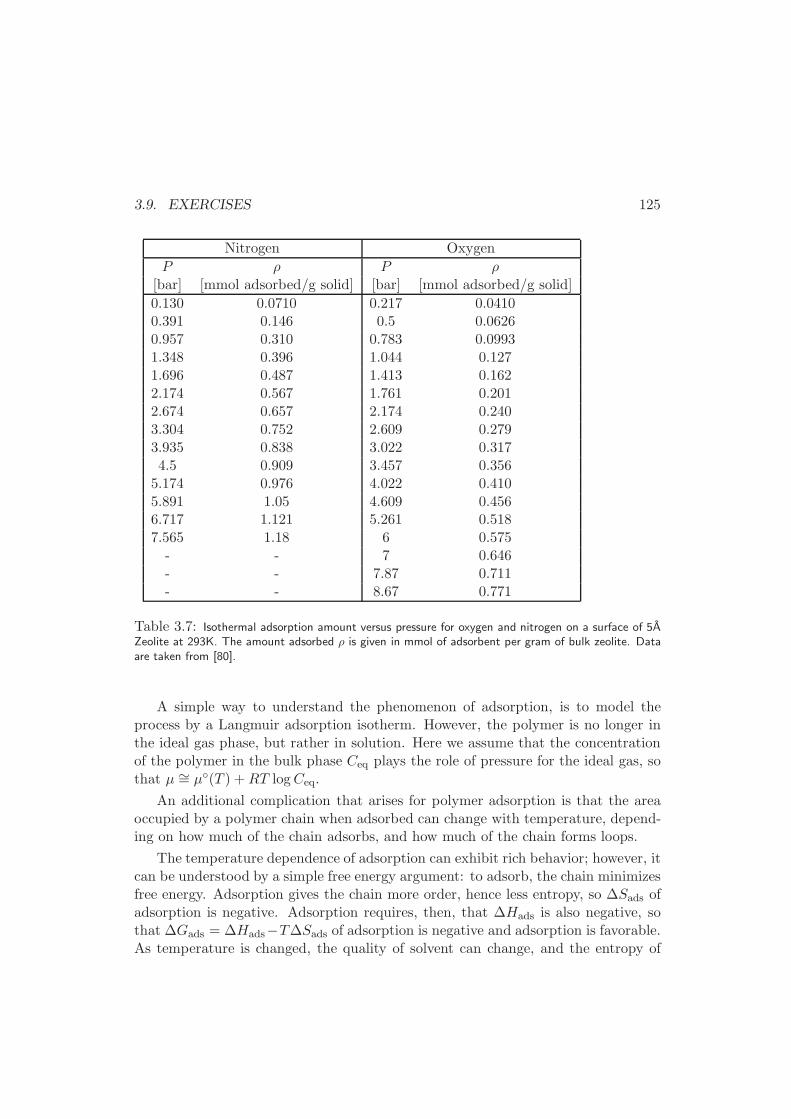
3.9. EXERCISES 125
Nitrogen Oxygen
P ρ P ρ[bar] [mmol adsorbed/g solid] [bar] [mmol adsorbed/g solid]
0.130 0.0710 0.217 0.04100.391 0.146 0.5 0.06260.957 0.310 0.783 0.09931.348 0.396 1.044 0.1271.696 0.487 1.413 0.1622.174 0.567 1.761 0.2012.674 0.657 2.174 0.2403.304 0.752 2.609 0.2793.935 0.838 3.022 0.3174.5 0.909 3.457 0.3565.174 0.976 4.022 0.4105.891 1.05 4.609 0.4566.717 1.121 5.261 0.5187.565 1.18 6 0.575- - 7 0.646- - 7.87 0.711- - 8.67 0.771
Table 3.7: Isothermal adsorption amount versus pressure for oxygen and nitrogen on a surface of 5AZeolite at 293K. The amount adsorbed ρ is given in mmol of adsorbent per gram of bulk zeolite. Dataare taken from [80].
A simple way to understand the phenomenon of adsorption, is to model theprocess by a Langmuir adsorption isotherm. However, the polymer is no longer inthe ideal gas phase, but rather in solution. Here we assume that the concentrationof the polymer in the bulk phase Ceq plays the role of pressure for the ideal gas, sothat µ ∼= µ(T ) +RT logCeq.
An additional complication that arises for polymer adsorption is that the areaoccupied by a polymer chain when adsorbed can change with temperature, depend-ing on how much of the chain adsorbs, and how much of the chain forms loops.
The temperature dependence of adsorption can exhibit rich behavior; however, itcan be understood by a simple free energy argument: to adsorb, the chain minimizesfree energy. Adsorption gives the chain more order, hence less entropy, so ∆Sads ofadsorption is negative. Adsorption requires, then, that ∆Hads is also negative, sothat ∆Gads = ∆Hads−T∆Sads of adsorption is negative and adsorption is favorable.As temperature is changed, the quality of solvent can change, and the entropy of
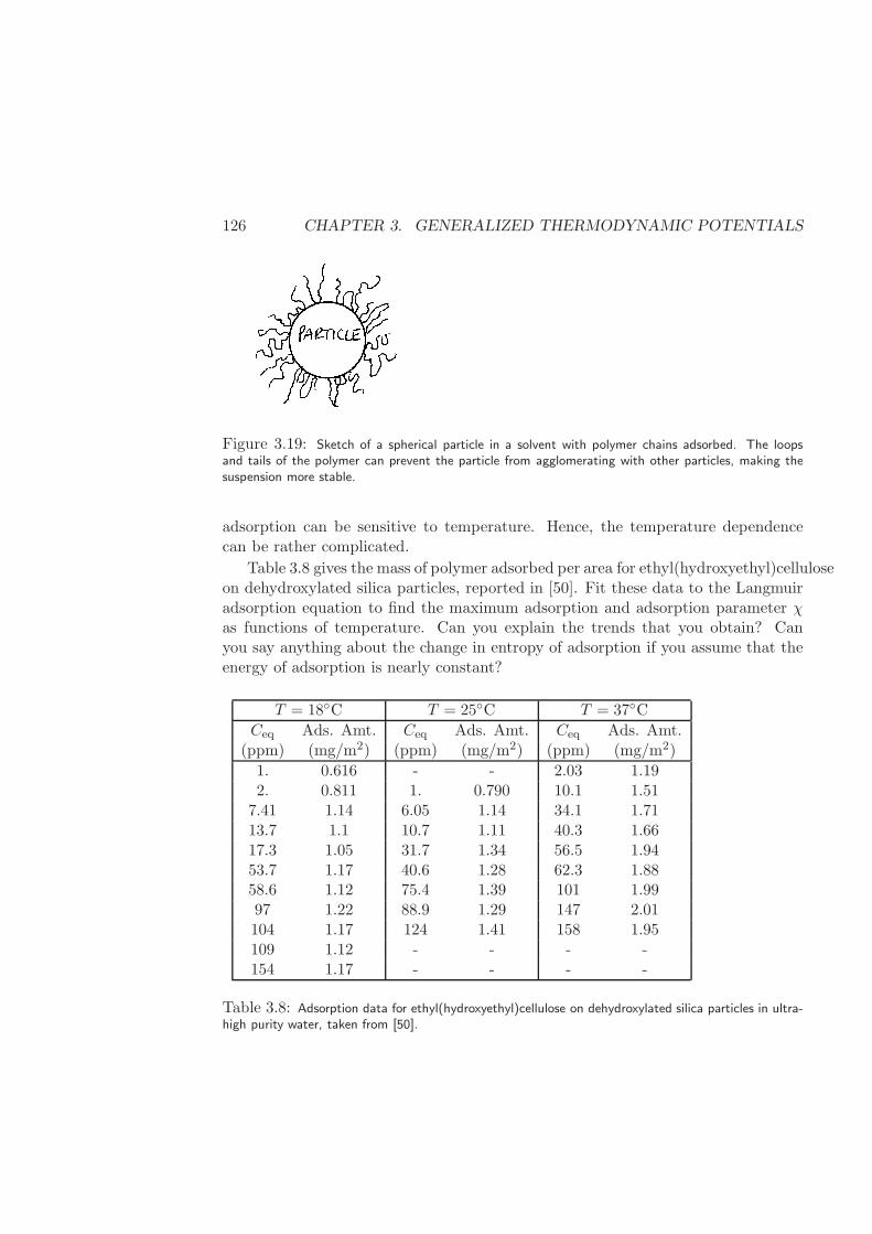
126 CHAPTER 3. GENERALIZED THERMODYNAMIC POTENTIALS
Figure 3.19: Sketch of a spherical particle in a solvent with polymer chains adsorbed. The loopsand tails of the polymer can prevent the particle from agglomerating with other particles, making thesuspension more stable.
adsorption can be sensitive to temperature. Hence, the temperature dependencecan be rather complicated.
Table 3.8 gives the mass of polymer adsorbed per area for ethyl(hydroxyethyl)celluloseon dehydroxylated silica particles, reported in [50]. Fit these data to the Langmuiradsorption equation to find the maximum adsorption and adsorption parameter χas functions of temperature. Can you explain the trends that you obtain? Canyou say anything about the change in entropy of adsorption if you assume that theenergy of adsorption is nearly constant?
T = 18C T = 25C T = 37CCeq Ads. Amt. Ceq Ads. Amt. Ceq Ads. Amt.
(ppm) (mg/m2) (ppm) (mg/m2) (ppm) (mg/m2)
1. 0.616 - - 2.03 1.192. 0.811 1. 0.790 10.1 1.51
7.41 1.14 6.05 1.14 34.1 1.7113.7 1.1 10.7 1.11 40.3 1.6617.3 1.05 31.7 1.34 56.5 1.9453.7 1.17 40.6 1.28 62.3 1.8858.6 1.12 75.4 1.39 101 1.9997 1.22 88.9 1.29 147 2.01104 1.17 124 1.41 158 1.95109 1.12 - - - -154 1.17 - - - -
Table 3.8: Adsorption data for ethyl(hydroxyethyl)cellulose on dehydroxylated silica particles in ultra-high purity water, taken from [50].
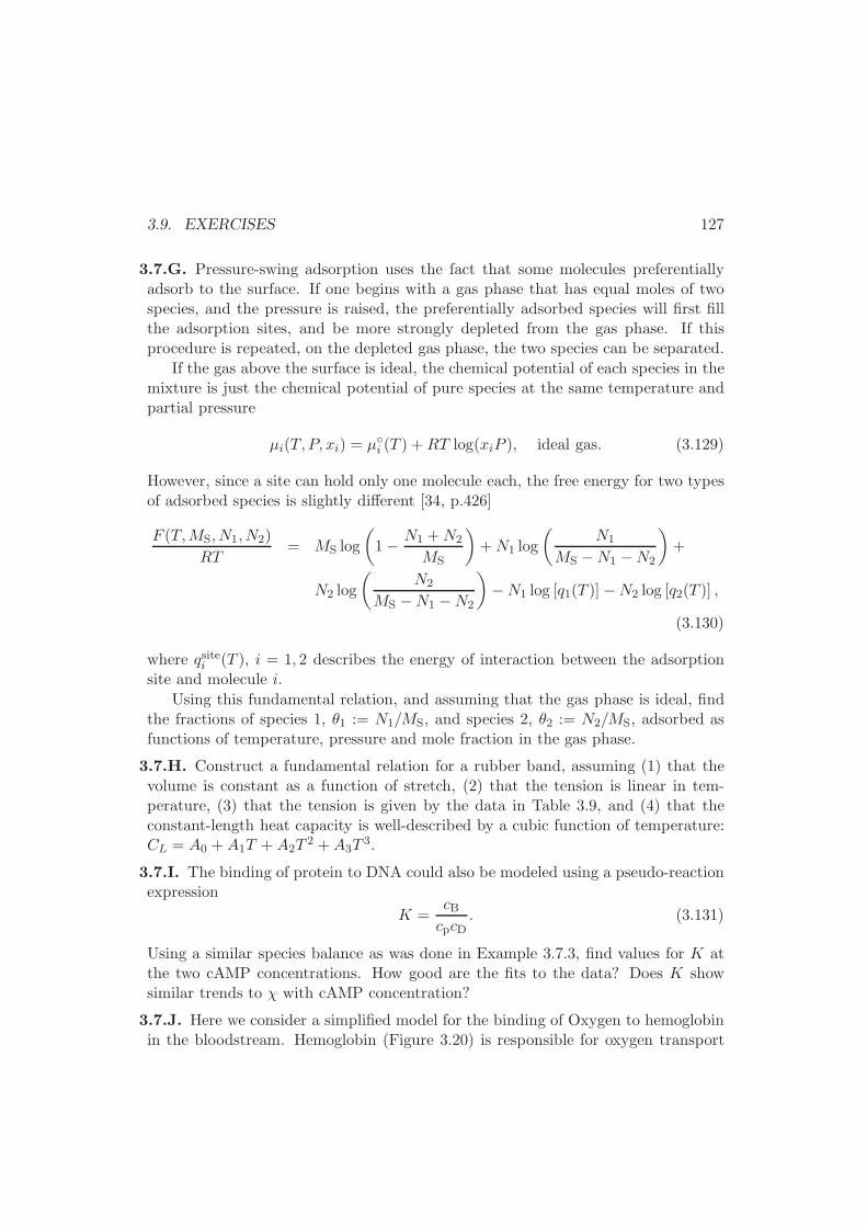
3.9. EXERCISES 127
3.7.G. Pressure-swing adsorption uses the fact that some molecules preferentiallyadsorb to the surface. If one begins with a gas phase that has equal moles of twospecies, and the pressure is raised, the preferentially adsorbed species will first fillthe adsorption sites, and be more strongly depleted from the gas phase. If thisprocedure is repeated, on the depleted gas phase, the two species can be separated.
If the gas above the surface is ideal, the chemical potential of each species in themixture is just the chemical potential of pure species at the same temperature andpartial pressure
µi(T, P, xi) = µi (T ) +RT log(xiP ), ideal gas. (3.129)
However, since a site can hold only one molecule each, the free energy for two typesof adsorbed species is slightly different [34, p.426]
F (T,MS, N1, N2)
RT= MS log
(
1− N1 +N2
MS
)
+N1 log
(N1
MS −N1 −N2
)
+
N2 log
(N2
MS −N1 −N2
)
−N1 log [q1(T )]−N2 log [q2(T )] ,
(3.130)
where qsitei (T ), i = 1, 2 describes the energy of interaction between the adsorptionsite and molecule i.
Using this fundamental relation, and assuming that the gas phase is ideal, findthe fractions of species 1, θ1 := N1/MS, and species 2, θ2 := N2/MS, adsorbed asfunctions of temperature, pressure and mole fraction in the gas phase.
3.7.H. Construct a fundamental relation for a rubber band, assuming (1) that thevolume is constant as a function of stretch, (2) that the tension is linear in tem-perature, (3) that the tension is given by the data in Table 3.9, and (4) that theconstant-length heat capacity is well-described by a cubic function of temperature:CL = A0 +A1T +A2T
2 +A3T3.
3.7.I. The binding of protein to DNA could also be modeled using a pseudo-reactionexpression
K =cBcpcD
. (3.131)
Using a similar species balance as was done in Example 3.7.3, find values for K atthe two cAMP concentrations. How good are the fits to the data? Does K showsimilar trends to χ with cAMP concentration?
3.7.J. Here we consider a simplified model for the binding of Oxygen to hemoglobinin the bloodstream. Hemoglobin (Figure 3.20) is responsible for oxygen transport
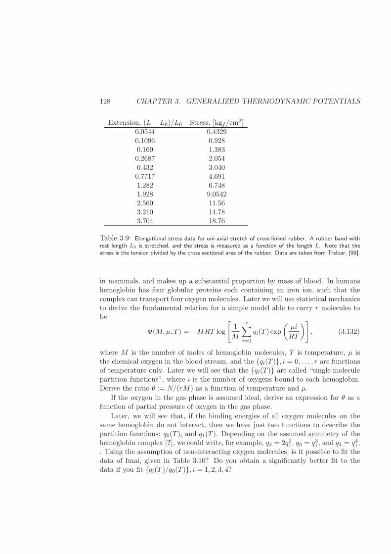
128 CHAPTER 3. GENERALIZED THERMODYNAMIC POTENTIALS
Extension, (L− L0)/L0 Stress, [kgf/cm2]
0.0544 0.43290.1096 0.9280.169 1.3830.2687 2.0540.432 3.0400.7717 4.6911.282 6.7481.928 9.05422.560 11.563.210 14.783.704 18.76
Table 3.9: Elongational stress data for uni-axial stretch of cross-linked rubber. A rubber band withrest length L0 is stretched, and the stress is measured as a function of the length L. Note that thestress is the tension divided by the cross sectional area of the rubber. Data are taken from Treloar, [99].
in mammals, and makes up a substantial proportion by mass of blood. In humanshemoglobin has four globular proteins each containing an iron ion, such that thecomplex can transport four oxygen molecules. Later we will use statistical mechanicsto derive the fundamental relation for a simple model able to carry r molecules tobe
Ψ(M,µ, T ) = −MRT log
[
1
M
r∑
i=0
qi(T ) exp
(µi
RT
)]
, (3.132)
where M is the number of moles of hemoglobin molecules, T is temperature, µ isthe chemical oxygen in the blood stream, and the qi(T ), i = 0, . . . , r are functionsof temperature only. Later we will see that the qi(T ) are called “single-moleculepartition functions”, where i is the number of oxygens bound to each hemoglobin.Derive the ratio θ := N/(rM) as a function of temperature and µ.
If the oxygen in the gas phase is assumed ideal, derive an expression for θ as afunction of partial pressure of oxygen in the gas phase.
Later, we will see that, if the binding energies of all oxygen molecules on thesame hemoglobin do not interact, then we have just two functions to describe thepartition functions: q0(T ), and q1(T ). Depending on the assumed symmetry of thehemoglobin complex [?], we could write, for example, q2 = 2q21, q3 = q31, and q4 = q41,. Using the assumption of non-interacting oxygen molecules, is it possible to fit thedata of Imai, given in Table 3.10? Do you obtain a significantly better fit to thedata if you fit qi(T )/q0(T ), i = 1, 2, 3, 4?
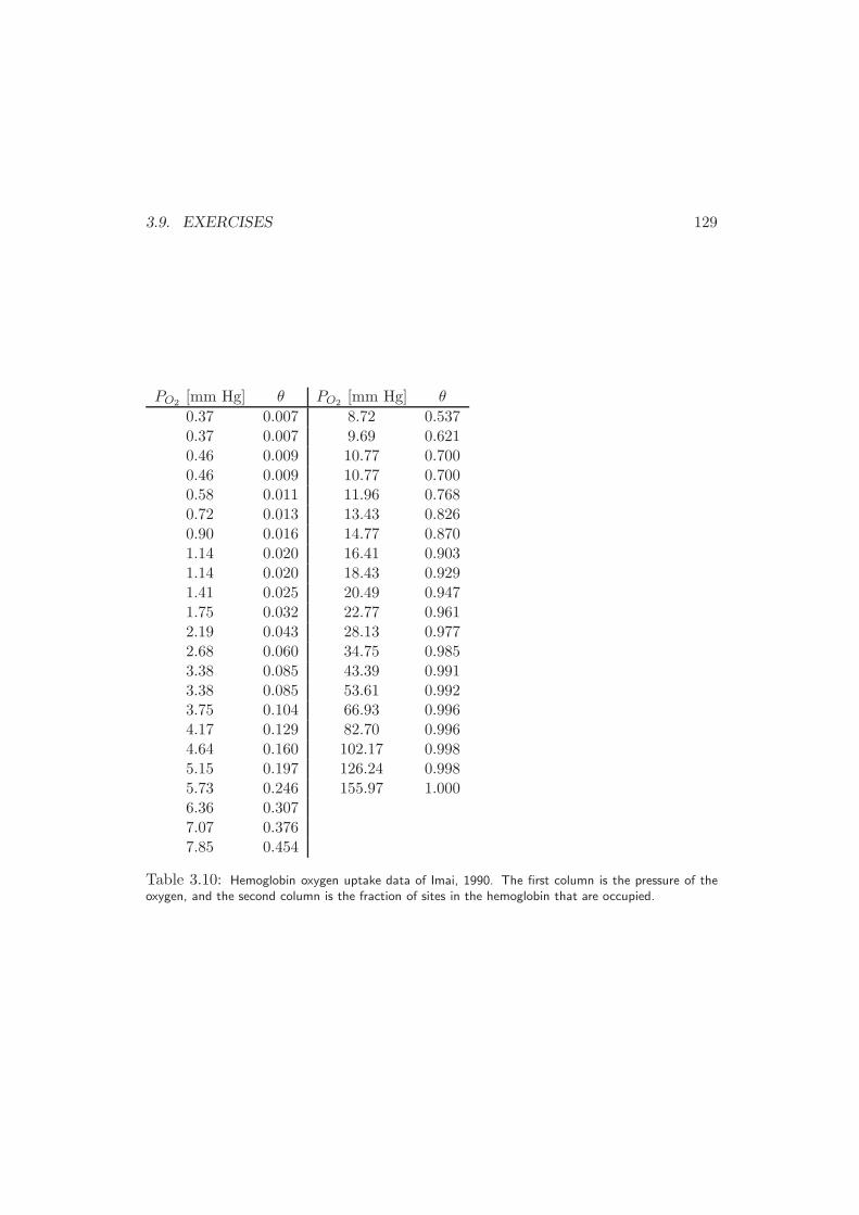
3.9. EXERCISES 129
PO2 [mm Hg] θ PO2 [mm Hg] θ
0.37 0.007 8.72 0.5370.37 0.007 9.69 0.6210.46 0.009 10.77 0.7000.46 0.009 10.77 0.7000.58 0.011 11.96 0.7680.72 0.013 13.43 0.8260.90 0.016 14.77 0.8701.14 0.020 16.41 0.9031.14 0.020 18.43 0.9291.41 0.025 20.49 0.9471.75 0.032 22.77 0.9612.19 0.043 28.13 0.9772.68 0.060 34.75 0.9853.38 0.085 43.39 0.9913.38 0.085 53.61 0.9923.75 0.104 66.93 0.9964.17 0.129 82.70 0.9964.64 0.160 102.17 0.9985.15 0.197 126.24 0.9985.73 0.246 155.97 1.0006.36 0.3077.07 0.3767.85 0.454
Table 3.10: Hemoglobin oxygen uptake data of Imai, 1990. The first column is the pressure of theoxygen, and the second column is the fraction of sites in the hemoglobin that are occupied.
130 CHAPTER 3. GENERALIZED THERMODYNAMIC POTENTIALS
3.7.K. A Mooney plot is often used to represent the tension of a rubber band understretch [?]. Here one plots the tension T divided by the stretch-dependence of thetension predicted by an ideal rubber band versus the inverse of the stretch ratioλ := L/L0. In this plot of T
2(λ2−1/λ)vs. 1/λ, one observes a significant region where
the data fall on a straight line with intercept C1 and slope C2. Find the fundamentalHelmholtz relation implied by this observation.
3.7.L. Consider a model polymer chain of N independent steps, each step of lengthaK. For a free, unconfined chain in a solvent, the Helmholtz potential F of the chainas a function of end-to-end length z can be well approximated by
Ffree(T, z,N) =3kBTz
2
Na2K(3.133)
where T is temperature and kB = R/NA is Boltzmann’s constant, NA is Avogadro’snumber, and R is the ideal gas constant. See Figure 3.21.
On the other hand, if the chain is tethered at one end to a solid, flat surface, asimple statistical mechanical argument estimates the Helmholtz potential to be
Fteth(T, z, r,N) =3kBT
(z2 + r2
)
Na2K− kBT log
(3z
NaK
)
(3.134)
where z is the perpendicular distance of the untethered end from the flat surface.The variable r is the radial distance from the line that runs perpendicular to thesurface, and passes through the tether, as shown on the right in the figure.
1. If the chain is pulled away from the flat surface a distance z, find the tensionTteth in the tethered chain. Find the similar tension Tfree in the untetheredchain to pull its end-to-end length a distance z apart.
2. Based on your results, make a sketch of the dimensionless tensions T aKkBT
, versusthe dimensionless length z
NKaKat a fixed temperature. Make the sketch as
quantitative as possible.
3. Explain where the approximations in the two models must break down, be-cause the results are no longer physical.
4. How much work does it take to stretch the tethered chain from z =√
N/3 aKto z = NaK/3 isothermally?
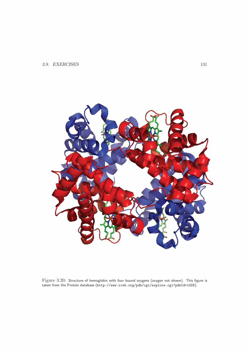
3.9. EXERCISES 131
Figure 3.20: Structure of hemoglobin with four bound oxygens (oxygen not shown). This figure istaken from the Protein database (http://www.rcsb.org/pdb/cgi/explore.cgi?pdbId=1GZX).
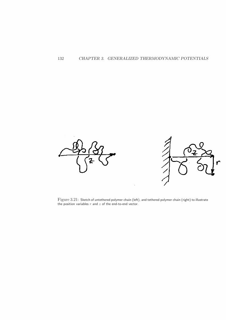
132 CHAPTER 3. GENERALIZED THERMODYNAMIC POTENTIALS
Figure 3.21: Sketch of untethered polymer chain (left), and tethered polymer chain (right) to illustratethe position variables r and z of the end-to-end vector.
Chapter 4
First Applications ofThermodynamics
What is astonishing in the realm of science is the oppositeof what is astonishing in the art of the conjurer. For thelatter wants to persuade us to see a very simple causality
where in truth a very complicated causality is at work. Science,on the contrary, compels us to abandon belief in simple causalities
precisely where everything seems so easy to comprehend and weare the fools of appearance. The ‘simplest’ things are very
complicated—a fact at which one can never cease to marvel!– Friedrich Nietzsche [63, Aphorism I:6]
Now that we have a reasonably complete structure of thermodynamics, we cantackle more complicated problems. In the following section we introduce the con-cepts of local and global stability, and show how local stability puts restrictions onsecond-order derivatives. In §4.2 we see that application of local stability criteriato proposed fundamental relations leads to predictions of spinodal curves, whichindicate when substances will spontaneously change state. Application of globalstability in §4.2.2 to a van der Waals fluid leads to predictions of vapor saturationcurves and liquid saturation curves. These latter curves are sometimes called bin-odal curves (or coexistence curves) and can be predicted from PV T equationsof state alone. We then show how thermodynamic diagrams useful for refrigeration,or power cycle design, can be constructed from PV T relations in §4.4. §4.4.2 showsgenerically how one can make predictions of differences in thermodynamic quantitiesfrom any of the equations of state shown in Appendix B or from experimental data.
133
134 CHAPTER 4. FIRST APPLICATIONS OF THERMODYNAMICS
4.1 Stability Criteria
What happens if you take gaseous nitrogen and compress it, keeping the internalenergy constant by removing heat? Eventually, the nitrogen begins to condensein the container, and you have a mixture of liquid and gaseous nitrogen. If youisolate this system and wait for a long time, then you see that the system is indeedat a stable equilibrium. From §2.8 we know that these two phases have the sametemperature and pressure. How can that be? Why is some of the nitrogen happyto stay gaseous, while the rest saw fit to condense into a liquid? Both phaseshave the same temperature and pressure, yet they have different densities. If wecompress the fluid more, we find that these two phases are always present and haveconstant specific volume—further compression changes only the relative amounts ofeach phase. Why does the fluid not change the density of one or both phases? Theanswer to these questions comes from the concept of stability.
Because a real system is made up of discrete particles such as atoms and molecules,the density of a fluid in some region of the system is always fluctuating. If we dividea system into two equal-sized halves, each subdivision will have the same number ofmolecules on average. However, at any instant of time, one side may have severalmore molecules than the other. This would be a fluctuation in density. Similarly,there will be fluctuations in energy. It is possible that the entropy of the total systemgrows from one of these fluctuations. If so, we say that the system is unstable—as required by the fourth postulate. Since the fluctuations are unconstrained, anyfluctuation that increases the entropy will continue to grow, according to the fourthpostulate.
If the entropy grows for any size fluctuation, no matter how small, we say thatthe system is locally unstable. If a single molecule imbalance raises the entropy,the system is locally unstable. However, if a fluctuation requires a certain finite sizeto find the state of higher entropy, we call the system globally unstable. Maybethe difference in densities of the two sides needs to be larger than some minimumnumber. If the entropy never grows for any size of fluctuation, then the system isstable.
The first section of this chapter derives the stability criteria for simple systems.The second section applies these criteria to predict the vapor-liquid equilibrium ofpure substances using PvT equations of state.
4.1.1 Entropy
Recall that the second law states that the unconstrained variables of a system ar-range themselves such as to maximize the entropy. We put N moles of a fluid in arigid container of volume V , and insulate it so that its internal energy stays fixed at
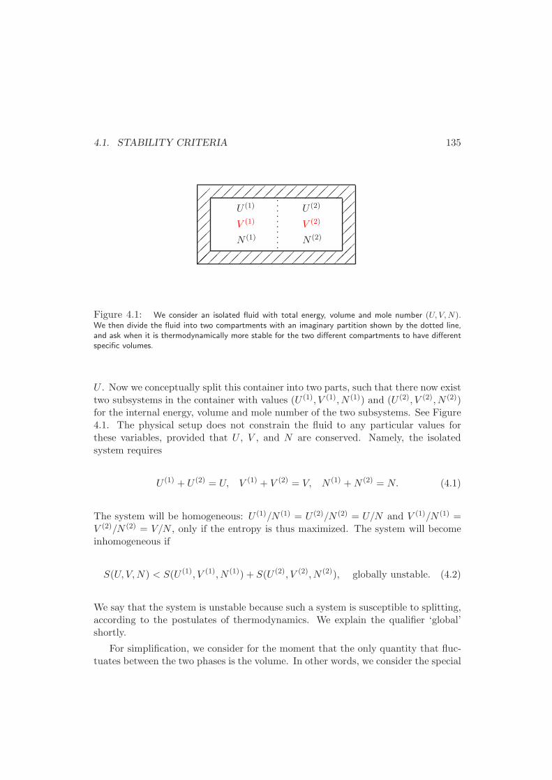
4.1. STABILITY CRITERIA 135
U (1) U (2)
V (1) V (2)
N (1) N (2)..........
Figure 4.1: We consider an isolated fluid with total energy, volume and mole number (U, V,N).We then divide the fluid into two compartments with an imaginary partition shown by the dotted line,and ask when it is thermodynamically more stable for the two different compartments to have differentspecific volumes.
U . Now we conceptually split this container into two parts, such that there now existtwo subsystems in the container with values (U (1), V (1), N (1)) and (U (2), V (2), N (2))for the internal energy, volume and mole number of the two subsystems. See Figure4.1. The physical setup does not constrain the fluid to any particular values forthese variables, provided that U , V , and N are conserved. Namely, the isolatedsystem requires
U (1) + U (2) = U, V (1) + V (2) = V, N (1) +N (2) = N. (4.1)
The system will be homogeneous: U (1)/N (1) = U (2)/N (2) = U/N and V (1)/N (1) =V (2)/N (2) = V/N , only if the entropy is thus maximized. The system will becomeinhomogeneous if
S(U, V,N) < S(U (1), V (1), N (1)) + S(U (2), V (2), N (2)), globally unstable. (4.2)
We say that the system is unstable because such a system is susceptible to splitting,according to the postulates of thermodynamics. We explain the qualifier ‘global’shortly.
For simplification, we consider for the moment that the only quantity that fluc-tuates between the two phases is the volume. In other words, we consider the special
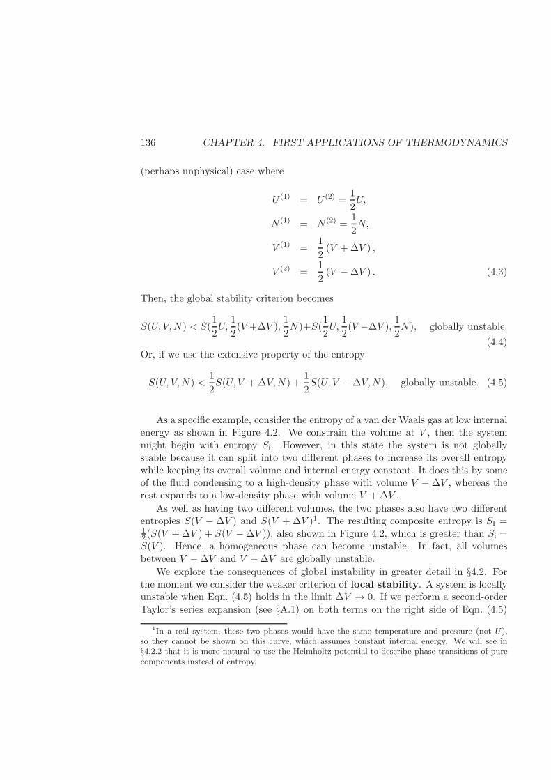
136 CHAPTER 4. FIRST APPLICATIONS OF THERMODYNAMICS
(perhaps unphysical) case where
U (1) = U (2) =1
2U,
N (1) = N (2) =1
2N,
V (1) =1
2(V +∆V ) ,
V (2) =1
2(V −∆V ) . (4.3)
Then, the global stability criterion becomes
S(U, V,N) < S(1
2U,
1
2(V +∆V ),
1
2N)+S(
1
2U,
1
2(V −∆V ),
1
2N), globally unstable.
(4.4)Or, if we use the extensive property of the entropy
S(U, V,N) <1
2S(U, V +∆V,N) +
1
2S(U, V −∆V,N), globally unstable. (4.5)
As a specific example, consider the entropy of a van der Waals gas at low internalenergy as shown in Figure 4.2. We constrain the volume at V , then the systemmight begin with entropy Si. However, in this state the system is not globallystable because it can split into two different phases to increase its overall entropywhile keeping its overall volume and internal energy constant. It does this by someof the fluid condensing to a high-density phase with volume V −∆V , whereas therest expands to a low-density phase with volume V +∆V .
As well as having two different volumes, the two phases also have two differententropies S(V − ∆V ) and S(V + ∆V )1. The resulting composite entropy is SI =12(S(V +∆V ) + S(V −∆V )), also shown in Figure 4.2, which is greater than Si =S(V ). Hence, a homogeneous phase can become unstable. In fact, all volumesbetween V −∆V and V +∆V are globally unstable.
We explore the consequences of global instability in greater detail in §4.2. Forthe moment we consider the weaker criterion of local stability. A system is locallyunstable when Eqn. (4.5) holds in the limit ∆V → 0. If we perform a second-orderTaylor’s series expansion (see §A.1) on both terms on the right side of Eqn. (4.5)
1In a real system, these two phases would have the same temperature and pressure (not U),so they cannot be shown on this curve, which assumes constant internal energy. We will see in§4.2.2 that it is more natural to use the Helmholtz potential to describe phase transitions of purecomponents instead of entropy.
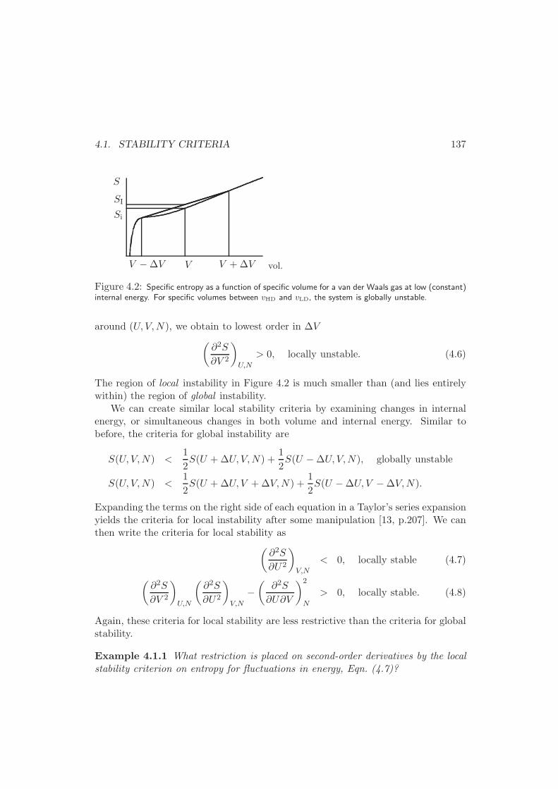
4.1. STABILITY CRITERIA 137
S
vol.V −∆V V +∆VV
Si
SI
Figure 4.2: Specific entropy as a function of specific volume for a van der Waals gas at low (constant)internal energy. For specific volumes between vHD and vLD, the system is globally unstable.
around (U, V,N), we obtain to lowest order in ∆V
(∂2S
∂V 2
)
U,N
> 0, locally unstable. (4.6)
The region of local instability in Figure 4.2 is much smaller than (and lies entirelywithin) the region of global instability.
We can create similar local stability criteria by examining changes in internalenergy, or simultaneous changes in both volume and internal energy. Similar tobefore, the criteria for global instability are
S(U, V,N) <1
2S(U +∆U, V,N) +
1
2S(U −∆U, V,N), globally unstable
S(U, V,N) <1
2S(U +∆U, V +∆V,N) +
1
2S(U −∆U, V −∆V,N).
Expanding the terms on the right side of each equation in a Taylor’s series expansionyields the criteria for local instability after some manipulation [13, p.207]. We canthen write the criteria for local stability as
(∂2S
∂U2
)
V,N
< 0, locally stable (4.7)
(∂2S
∂V 2
)
U,N
(∂2S
∂U2
)
V,N
−(
∂2S
∂U∂V
)2
N
> 0, locally stable. (4.8)
Again, these criteria for local stability are less restrictive than the criteria for globalstability.
Example 4.1.1 What restriction is placed on second-order derivatives by the localstability criterion on entropy for fluctuations in energy, Eqn. (4.7)?
138 CHAPTER 4. FIRST APPLICATIONS OF THERMODYNAMICS
Solution: We note that we can write the left side of Eqn. (4.7) as
(∂2S
∂U2
)
V,N
=
(∂
∂U
(∂S
∂U
)
V
)
V
= − 1
T 2
(∂T
∂U
)
V
= − 1
T 2(∂U∂T
)
V
= − 1
T 3(∂S∂T
)
V
where the second line follows from the definition of temperature, and the restare standard thermodynamic manipulations shown in §3.6. Note that the de-nominator in the fraction of the last line is simply T 2CV , where CV is calledthe constant-volume heat capacity. Thus, the local stability criterionEqn. (4.7) then says that the constant-volume heat capacity must be positive
CV := T
(∂S
∂T
)
V
> 0, locally stable, (4.9)
otherwise, the system will split into two phases, and each phase will have pos-itive constant-volume heat capacity. 2
Note that the requirement found in this example is independent of the specificmodel for fundamental energy used to describe the system—it is a result strictlyof the postulates of thermodynamics. Interpretation of the other local stabilityrelations is more easily handled using the generalized potentials in §4.1.3, which wecover shortly.
4.1.2 Internal Energy
We may also look at stability criteria when other variables are manipulated instead of(U, V ). For example, if we manipulate entropy and volume, it is natural to considerinternal energy as the dependent variable. In §3.2 we found that an equilibriumstate is attained when internal energy is minimized at constant entropy. If we makelocal stability arguments for U analogous to those that we made for S, we find thatlocal stability requires
(∂2U∂S2
)
V,N> 0
(∂2U∂V 2
)
S,N> 0
(∂2U∂V 2
)
S,N
(∂2U∂S2
)
V,N−(∂2U∂S∂V
)2
N> 0
locally stable. (4.10)
4.1. STABILITY CRITERIA 139
Manipulation of the first two derivatives leads to the requirements that
CV := T
(∂S
∂T
)
V
> 0, κS := − 1
V
(∂V
∂P
)
S
> 0, local stability, (4.11)
where κS is the isentropic compressibility.
4.1.3 Generalized Potentials
Not surprisingly, the generalized potentials also satisfy extremum conditions at equi-librium. Using the properties of Legendre transforms, it is possible to show (also seeProblem 4.1.C and Problem 4.1.D) that the conditions for local stability are
(∂2H∂S2
)
P,N> 0,
(∂2H∂P 2
)
S,N< 0
(∂2F∂T 2
)
V,N< 0,
(∂2F∂V 2
)
T,N> 0
(∂2G∂T 2
)
P,N< 0,
(∂2G∂P 2
)
T,N< 0
locally stable. (4.12)
Example 4.1.2 Prove the second stability criterion for H.
Solution: From Table 3.1 we know that
V =
(∂H
∂P
)
S
.
Taking the derivative of each side with respect to P holding S constant yields
(∂V
∂P
)
S
=
(∂2H
∂P 2
)
S
.
However, from the definition of pressure, we also know that
(∂P
∂V
)
S
= −(∂2U
∂V 2
)
S
,
whence(∂2H
∂P 2
)
S
= −1
/(∂2U
∂V 2
)
S
.
Hence, the stability for enthalpy to fluctuations in pressure has sign oppositeto that for internal energy to fluctuations in volume. Combining this equationwith the stability criterion for U , Eqn. (4.10) yields the second relation in thefirst line of Eqn. (4.12). 2
140 CHAPTER 4. FIRST APPLICATIONS OF THERMODYNAMICS
Note that in all cases, stability to fluctuations in an extensive variable are min-ima, and those in intensive variables are maxima. Manipulation of the second sta-bility criterion for F leads to the requirement (Problem 4.1.B) that
κT > 0, (4.13)
an important criterion in constructing phase diagrams for pure component systems,as will be seen in §4.2.
In Example 3.6.3 we found a relationship between theRestrictions
CP > CV > 0κT > κS > 0
Table 4.1: Restrictionson second-order deriva-tives from stability consid-erations.
constant-volume heat capacity and constant-pressure heatcapacity. Using Eqn. (3.85) and stability condition Eqn. (4.11)we find that
CP = CV +V α2T
κT> CV > 0. (4.14)
Similarly, using the techniques of §3.6, and Eqn. (4.11), wefind
κT =CPCV
κS > κS > 0. (4.15)
The physical interpretation of these results is straightforward. Increasing thetemperature of a system at constant pressure or volume necessarily increases itsentropy, which means that heat must be added. Also, increasing the pressure of asystem at either constant temperature or constant entropy necessarily decreases itsvolume. The results are summarized in Table 4.1.
Finally, we can now prove the fourth relation for temperature that we promisedon p.39. From the differential for internal energy, we can prove that
(∂U
∂T
)
V,N
= CV > 0.
Since the constant-volume heat capacity must be positive by stability, raising thetemperature at constant volume necessarily increases the internal energy of a sub-stance.
4.2 Single Component Vapor-Liquid Equilibrium
Sometimes we have little information about the fundamental relation for a substance,but we know a great deal about its mechanical equation of state. For example, wemay know its PV T behavior over a wide range of temperatures and pressures, orwe may use statistical mechanical arguments to derive such an expression. In this
4.2. SINGLE COMPONENT VAPOR-LIQUID EQUILIBRIUM 141
section we show how such information is sufficient to understand the phase stabilityof single component systems. By studying the phase stability, we can use equationsof state to predict the vapor saturation line and liquid saturation line for purecomponent systems (the binodal curve). An equation of state that describes boththe liquid and the vapor phases of a substance is called an equation of state for afluid.
Rather than give the general principles involved in such manipulations, we beginwith an example of the van der Waals fluid. The procedure used to reveal the phasebehavior of a van der Waals fluid is general for any fluid, and the general procedureis outlined at the conclusion of this section, in subsection §4.2.3.
4.2.1 Spinodal curve of a van der Waals fluid
The ideal gas model assumes that molecules consist of point particles that do notinteract with each other. From statistical mechanics, it is known that the pressurecan be expressed as a sum of repulsive and attractive intermolecular contributions.A simple expression for the repulsive contributions can be obtained by analyzing thebehavior of the molar volume in the limit of infinite pressure; the ideal gas equationof state predicts that the volume should vanish. At high pressures, however, weexpect most fluids to solidify; a reasonable model for a fluid should therefore reachan asymptotic volume beyond which it can no longer be compressed. That deficiencycan be corrected by assuming that the repulsive part of the pressure is given by
P =RT
v − b, (4.16)
where b can be interpreted as the molar volume that the fluid would have in thelimit of infinite pressure. At constant temperature, Eqn. (4.16) predicts a monotonicdecrease of the volume with pressure. As v approaches b, the pressure diverges.
We also know that atoms consist of electrons and protons, which interact witheach other according to Coulomb’s law; assuming that interactions between differentatoms are pairwise additive, the pressure of a fluid is expected to decrease (below thepurely repulsive value) by an amount proportional to the square of the density. Byconsidering both attractive and repulsive contributions a simple mechanical equationof state can be written in the form
P =RT
v − b− a
v2. (4.17)
Eqn. (4.17) is the familiar van der Waals equation of state, Eqn. (2.35). It was firstproposed by Johannes Diderik van der Waals in his doctoral thesis more than ahundred years ago [102]. In spite of its simplicity, this equation is able to capture
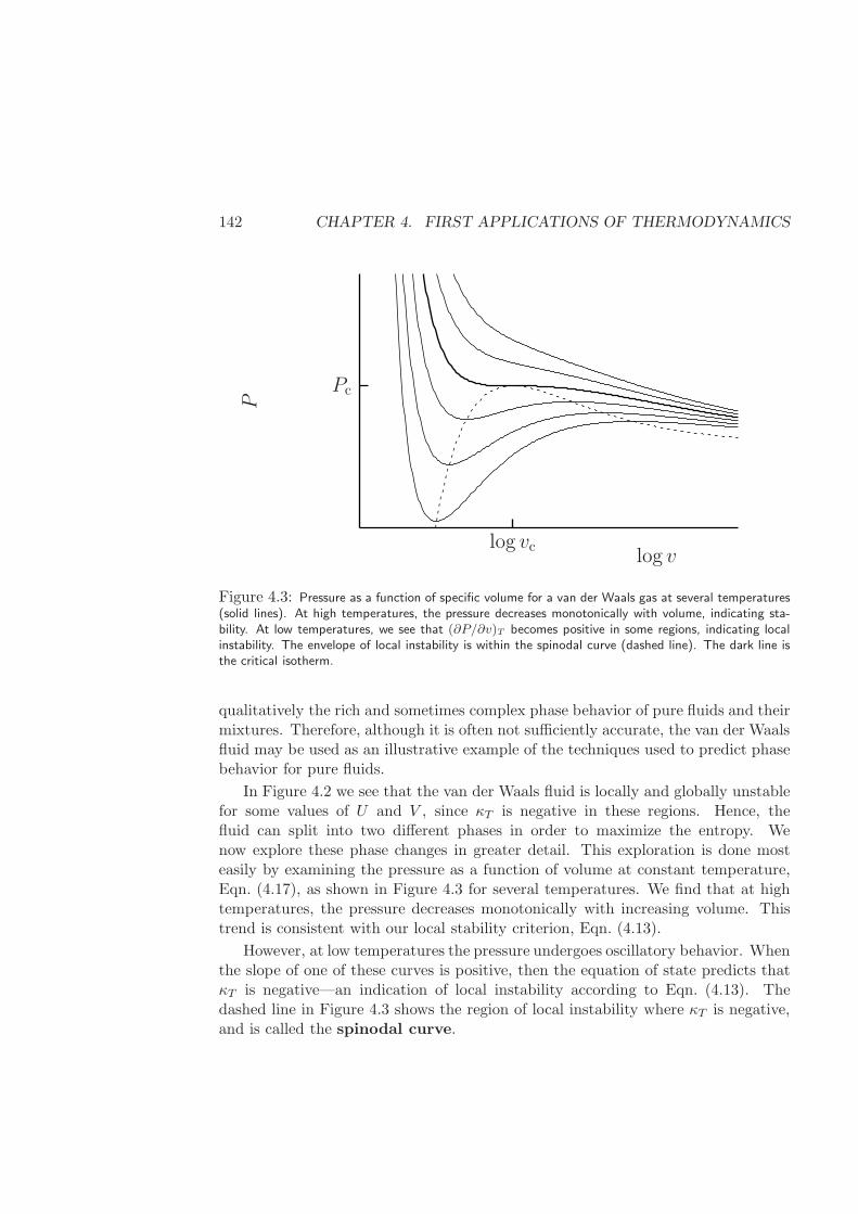
142 CHAPTER 4. FIRST APPLICATIONS OF THERMODYNAMICS
log v
P
log vc
Pc
Figure 4.3: Pressure as a function of specific volume for a van der Waals gas at several temperatures(solid lines). At high temperatures, the pressure decreases monotonically with volume, indicating sta-bility. At low temperatures, we see that (∂P/∂v)T becomes positive in some regions, indicating localinstability. The envelope of local instability is within the spinodal curve (dashed line). The dark line isthe critical isotherm.
qualitatively the rich and sometimes complex phase behavior of pure fluids and theirmixtures. Therefore, although it is often not sufficiently accurate, the van der Waalsfluid may be used as an illustrative example of the techniques used to predict phasebehavior for pure fluids.
In Figure 4.2 we see that the van der Waals fluid is locally and globally unstablefor some values of U and V , since κT is negative in these regions. Hence, thefluid can split into two different phases in order to maximize the entropy. Wenow explore these phase changes in greater detail. This exploration is done mosteasily by examining the pressure as a function of volume at constant temperature,Eqn. (4.17), as shown in Figure 4.3 for several temperatures. We find that at hightemperatures, the pressure decreases monotonically with increasing volume. Thistrend is consistent with our local stability criterion, Eqn. (4.13).
However, at low temperatures the pressure undergoes oscillatory behavior. Whenthe slope of one of these curves is positive, then the equation of state predicts thatκT is negative—an indication of local instability according to Eqn. (4.13). Thedashed line in Figure 4.3 shows the region of local instability where κT is negative,and is called the spinodal curve.
4.2. SINGLE COMPONENT VAPOR-LIQUID EQUILIBRIUM 143
There is a unique point in this plot that corresponds to the maximum in the spin-odal curve called the critical point.2 The isotherm that passes through this pointis called the critical isotherm, with critical temperature Tc. Correspondingly,there is a critical pressure Pc, and a critical volume vc. When the temperatureis above Tc, the volume decreases monotonically with pressure, a so-called super-critical fluid. Super-critical fluids are neither gases nor liquids; when compressedisothermally, their density changes smoothly, and they undergo no phase change.Fluids near the critical point have some very interesting properties which we waituntil §6.7 to discuss. For the moment we are interested in temperatures below Tc,where the fluid can be either a gas or a liquid, depending on the pressure and volume.
First, we find the critical variables for the van der Waals fluid of Figure 4.3.The criterion for local instability is
(∂P∂v
)
T> 0. The spinodal curve is where the
system goes from stable to unstable. Hence, we can find the spinodal point at agiven volume by finding where
(∂P∂v
)
T= 0 or κT = 0 from Eqn. (4.17). When we
set the derivative to zero and solve for the spinodal temperature, we obtain
RTs(v) =2a(v − b)2
v3, (4.18)
where Ts(v) is the spinodal temperature as a function of volume. Inserting theexpression for the spinodal temperature Eqn. (4.18) into the van der Waals equationof state, Eqn. (4.17), we obtain an expression for the spinodal curve
Ps(v) =a
v2
(
1− 2b
v
)
. (4.19)
This is the equation used to plot the dashed line in Figure 4.3. We can now find thecritical point by finding the maximum of this curve. Taking the derivative of eachside of Eqn. (4.19) with respect to volume, we obtain
dPs
dv=
2a
v3
(3b
v− 1
)
. (4.20)
Clearly, the derivative is zero when the volume is 3b, to give the critical volume
vc = 3b, van der Waals fluid. (4.21)
The critical pressure is found from the spinodal curve, Eqn. (4.19), and the criticaltemperature from the spinodal temperature, Eqn. (4.18) at the critical volume
2According to Sengers and Levelt [88], James Clerk Maxwell and Diederek Johannes Kortewegcredit Arthur Cayley as being the first to define the critical point.

144 CHAPTER 4. FIRST APPLICATIONS OF THERMODYNAMICS
Pc = Ps(vc) = a27b2 ,
Tc = Ts(vc) = 8a27Rb .
van der Waals fluid. (4.22)
Using these relations, we can eliminate constants in the van der Waals equation ofstate Eqn. (4.17) to express it in reduced form
Pr =8Tr
3vr − 1− 3
v2r, van der Waals fluid. (4.23)
where we have defined the reduced variables
Tr :=T
Tc, reduced temperature, (4.24)
Pr :=P
Pc, reduced pressure, (4.25)
vr :=v
vc, reduced volume. (4.26)
We have now completely characterized the region of local instability for the van derWaals fluid. Also, by introducing reduced variables, we have a universal expressionfor the PV T behavior of all fluids, insofar as they are described by the van der Waalsfluid. There are many such equations of state that predict such universal behaviorfor fluids, called corresponding states models. This means that if you plot thePV T data for many fluids in terms of reduced quantities, the data should lie ontop of one another for different materials. Such behavior is observed approximatelyfor a number of simple chemical species, even though they do not obey well thevan der Waals equation of state. The relationships for some fluids, like water, withspecial molecular associations (called hydrogen bonding) do not fit with those ofthe other, simple fluids.
Note that the van der Waals fluid predicts a universal value of the critical com-pressibility factor
zc :=PcvcRTc
=3
8, van der Waals fluid, (4.27)
where the compressibility factor z is defined for a non-ideal fluid as
z :=PV
NRT. (4.28)
However, we know experimentally that fluids exhibit a range of critical compress-ibility factors typically below ≈ 0.3. Hence, the van der Waals fluid is not capableof capturing the PV T relations of a real fluid accurately near the critical region.
4.2. SINGLE COMPONENT VAPOR-LIQUID EQUILIBRIUM 145
The region of global instability is larger than, and entirely encompasses theregion of local instability; the curve demarcating the line of global instability iscalled the binodal curve (not shown in Figure 4.3). In the locally unstable region,the material will spontaneously phase separate without external influence. However,in the region that is globally unstable, but locally stable, a system free of externalperturbation may remain for long periods of time as a single phase. For example,there have been news reports about the dangers of heating water in a microwaveoven. Water placed in a ceramic mug and heated sufficiently long in the oven (anisobaric process), can be put inside the binodal curve, but outside the spinodalcurve. If the mug is not perturbed, the water may stay liquid, although this is onlymetastable. When the oven user removes the mug and adds a teabag, spoon, or justperturbs the water, it may suddenly and rapidly boil, dousing the holder of the mugwith scalding water.
Analogously, a fluid may sometimes be cooled very slowly and carefully below itsfreezing point without crystallizing. However, when the container is tapped from theoutside, the entire fluid may crystallize extremely rapidly. Such a supersaturatedliquid is an example of a substance that is inside the binodal curve, but outside thespinodal curve. Once the temperature is lowered sufficiently to bring the substanceto the spinodal curve, crystallization will occur spontaneously, even if the materialis kept vibration free.
These properties are exploited in engineering practice when producing crystals.If a system is kept between the binodal and spinodal curves crystallization beginsat a single point, or at very few points in the liquid. However, if quenched to apoint inside the spinodal region, crystallization is nucleated at many points. In thelatter case, many tiny crystals form. However, in the former situation it is possibleto produce very large crystals of high purity. Such large crystals are necessary forX-ray crystallography to study conformational properties of proteins, for example.
4.2.2 Binodal (or Coexistence) curve of a van der Waals fluid
Consider a sub-critical isotherm of a van der Waals vapor in Figure 4.4. The ther-modynamic state of the vapor would be on a point in the lower right-hand cornerof the figure, and would have low density; in other words, the fluid would be a gas.Now begin to increase the pressure gradually, holding the temperature constant.The evolution of the thermodynamic state of the system may be represented by apoint moving slowly along the sub-critical isotherm from right to left. Before reach-ing the region of local instability, marked by the spinodal curve, the point will firstreach the binodal curve, which envelopes the region of global stability. Physically,this corresponds to the point where the fluid begins to condense; most of the fluidis still a gas, but a tiny amount becomes liquid.
146 CHAPTER 4. FIRST APPLICATIONS OF THERMODYNAMICS
Since these two phases are in thermal, mechanical and chemical contact, theymust satisfy the equilibrium conditions found in Chapter 2
Tv = Tl,
Pv = Pl,
µv = µl,
where the subscripts indicate vapor or liquid. These are Eqs. (2.69) through (2.71)rewritten for vapor and liquid phases in contact. The pressure at which the liquidis in equilibrium with the vapor is called the saturation pressure P sat = Pv = Pl,and is unique for a given temperature.
Hence, the liquid phase in equilibrium with the vapor phase must lie on the sameisotherm as the vapor, and have the same pressure. A curve of constant pressureon this plot is a horizontal line. However, many horizontal lines may intersect withour sub-critical isotherm at three points. Which of these horizontal lines is thecorrect one is determined by the fact that the chemical potentials of the two phasesmust also be equal. We can find the location of the binodal curve from just themechanical equation of state and the equivalence of the chemical potentials in thefollowing way. The result is surprising: when the areas shown in Figure 4.4 areequal, the saturation pressure is found.
Recall that the chemical potential of a pure substance is just the specific Gibbsfree energy, Eqn. (3.21). We can find the change in Gibbs free energy (or chemicalpotential) as we change volume along the isotherm. At constant temperature thedifferential for the Gibbs potential, Eqn. (3.51), becomes
(∂µ
∂v
)
T,N
≡(∂g
∂v
)
T,N
= v
(∂P
∂v
)
T,N
, (4.29)
which also follows from the Gibbs-Duhem relation. If we integrate each side atconstant temperature from vv to vl, we obtain
µl − µv =
∫ vl
vv
v
(∂P
∂v
)
T,N
dv
0 = P sat (vl − vv)−∫ vl
vv
P dv
0 =
∫ vl
vv
[P sat(T )− P (T, v)
]dv. (4.30)
We integrated by parts to obtain the second line, and the fact that P sat is inde-pendent of volume to obtain the third. Since the left side is zero, the result has a
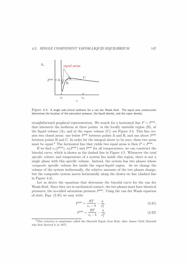
4.2. SINGLE COMPONENT VAPOR-LIQUID EQUILIBRIUM 147
C
BA
equal areas
v
P
vvvl
P sat
Figure 4.4: A single sub-critical isotherm for a van der Waals fluid. The equal area constructiondetermines the location of the saturation pressure, the liquid density, and the vapor density.
straightforward graphical representation. We search for a horizontal line P = P sat,that intersects the isotherm at three points: in the locally unstable region (B), atthe liquid volume (A), and at the vapor volume (C); see Figure 4.4. This line cre-ates two closed areas: one below P sat between points A and B, and one above P sat
between points B and C. In order for the integral above to be zero, these two areasmust be equal.3 The horizontal line that yields two equal areas is then P = P sat.
If we find vv(Psat), vl(P
sat) and P sat for all temperatures, we can construct thebinodal curve, which is shown as the dashed line in Figure 4.5. Whenever the totalspecific volume and temperature of a system lies inside this region, there is not asingle phase with this specific volume. Instead, the system has two phases whosecomposite specific volume lies inside the vapor-liquid region. As we change thevolume of the system isothermally, the relative amounts of the two phases change,but the composite system moves horizontally along the drawn tie line (dashed linein Figure 4.4).
Let us derive the equations that determine the binodal curve for the van derWaals fluid. Since they are in mechanical contact, the two phases must have identicalpressures, the so-called saturation pressure P sat. Using the van der Waals equationof state, Eqn. (2.35) we may write
P sat =RT
vv − b− a
v2v, (4.31)
P sat =RT
vl − b− a
v2l. (4.32)
3This criterion is sometimes called the Maxwell Equal Area Rule, after James Clerk Maxwellwho first derived it in 1875.
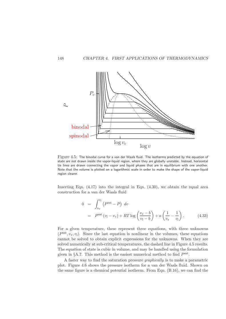
148 CHAPTER 4. FIRST APPLICATIONS OF THERMODYNAMICS
binodal
spinodal
log v
P
log vc
Pc
Figure 4.5: The binodal curve for a van der Waals fluid. The isotherms predicted by the equation ofstate are not drawn inside the vapor-liquid region, where they are globally unstable. Instead, horizontaltie lines are drawn connecting the vapor and liquid phases that are in equilibrium with one another.Note that the volume is plotted on a logarithmic scale in order to make the shape of the vapor-liquidregion clearer.
Inserting Eqn. (4.17) into the integral in Eqn. (4.30), we obtain the equal areaconstruction for a van der Waals fluid
0 =
∫ vl
vv
(P sat − P
)dv
= P sat (vl − vv) +RT log
(vv − b
vl − b
)
+ a
(1
vv− 1
vl
)
. (4.33)
For a given temperature, these represent three equations, with three unknowns(P sat, vv, vl). Since the last equation is nonlinear in the volumes, these equationscannot be solved to obtain explicit expressions for the unknowns. When they aresolved numerically at sub-critical temperatures, the dashed line in Figure 4.5 results.The equation of state is cubic in volume, and may be handled using the formulationgiven in §A.7. This method is the easiest numerical method to find P sat.
A faster way to find the saturation pressure graphically is to make a parametricplot. Figure 4.6 shows the pressure isotherm for a van der Waals fluid. Shown onthe same figure is a chemical potential isotherm. From Eqn. (B.16), we can find the
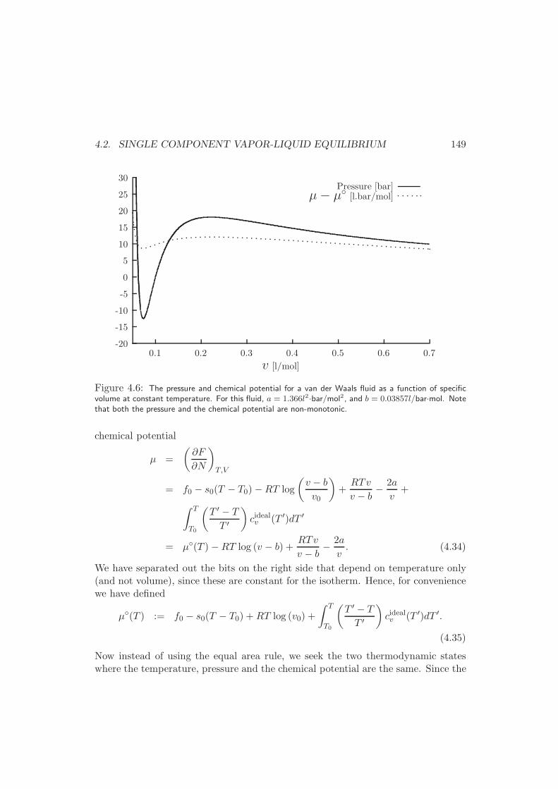
4.2. SINGLE COMPONENT VAPOR-LIQUID EQUILIBRIUM 149
-20
-15
-10
-5
0
5
10
15
20
25
30
0.1 0.2 0.3 0.4 0.5 0.6 0.7
v [l/mol]
Pressure [bar]µ− µ
[l.bar/mol]
Figure 4.6: The pressure and chemical potential for a van der Waals fluid as a function of specificvolume at constant temperature. For this fluid, a = 1.366l2·bar/mol2, and b = 0.03857l/bar·mol. Notethat both the pressure and the chemical potential are non-monotonic.
chemical potential
µ =
(∂F
∂N
)
T,V
= f0 − s0(T − T0)−RT log
(v − b
v0
)
+RTv
v − b− 2a
v+
∫ T
T0
(T ′ − T
T ′
)
cidealv (T ′)dT ′
= µ(T )−RT log (v − b) +RTv
v − b− 2a
v. (4.34)
We have separated out the bits on the right side that depend on temperature only(and not volume), since these are constant for the isotherm. Hence, for conveniencewe have defined
µ(T ) := f0 − s0(T − T0) +RT log (v0) +
∫ T
T0
(T ′ − T
T ′
)
cidealv (T ′)dT ′.
(4.35)
Now instead of using the equal area rule, we seek the two thermodynamic stateswhere the temperature, pressure and the chemical potential are the same. Since the
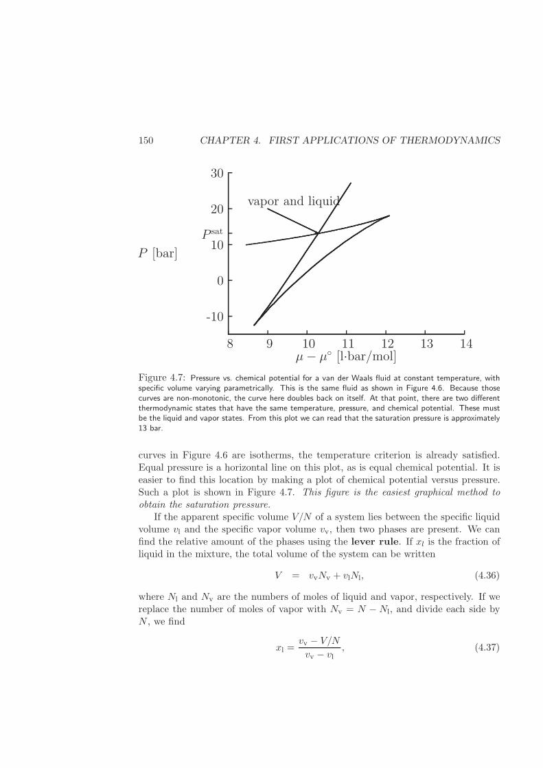
150 CHAPTER 4. FIRST APPLICATIONS OF THERMODYNAMICS
P sat
30
20
10
0
-10
8 9 10 11 12 13 14
P [bar]
µ− µ [l·bar/mol]
vapor and liquid
j
Figure 4.7: Pressure vs. chemical potential for a van der Waals fluid at constant temperature, withspecific volume varying parametrically. This is the same fluid as shown in Figure 4.6. Because thosecurves are non-monotonic, the curve here doubles back on itself. At that point, there are two differentthermodynamic states that have the same temperature, pressure, and chemical potential. These mustbe the liquid and vapor states. From this plot we can read that the saturation pressure is approximately13 bar.
curves in Figure 4.6 are isotherms, the temperature criterion is already satisfied.Equal pressure is a horizontal line on this plot, as is equal chemical potential. It iseasier to find this location by making a plot of chemical potential versus pressure.Such a plot is shown in Figure 4.7. This figure is the easiest graphical method toobtain the saturation pressure.
If the apparent specific volume V/N of a system lies between the specific liquidvolume vl and the specific vapor volume vv, then two phases are present. We canfind the relative amount of the phases using the lever rule. If xl is the fraction ofliquid in the mixture, the total volume of the system can be written
V = vvNv + vlNl, (4.36)
where Nl and Nv are the numbers of moles of liquid and vapor, respectively. If wereplace the number of moles of vapor with Nv = N − Nl, and divide each side byN , we find
xl =vv − V/N
vv − vl, (4.37)
4.2. SINGLE COMPONENT VAPOR-LIQUID EQUILIBRIUM 151
which has a straightforward graphical representation as a ratio of two lengths alonga tie line in Fig. 4.5.
In conclusion, we find that the fluid obeys the van der Waals equation of stateoutside the binodal curve, but follows the straight tie lines constructed inside thebinodal curve showing a mixture of vapor and liquid, as drawn in Figure 4.5. Thebehavior is qualitatively, but not quantitatively, correct. Better success can behad using the Peng-Robinson equation of state, or the Soave modification to theRedlich-Kwong equation of state (see Appendix B).
4.2.3 General Formulation
Given a PV T equation of state in the form P = P (v, T ), we can find the spinodalcurve Ps, saturation pressure P sat, vapor and liquid volumes vv and vl, for anytemperature, and the critical constants by the following relations.
The spinodal curve is determined by solution of the relation
(∂P
∂v
)
T
= 0. (4.38)
The critical point is determined by the simultaneous satisfaction of Eqn. (4.38),and the relation (
∂2P
∂v2
)
T
= 0. (4.39)
The vapor saturation line, the liquid saturation line and the saturation pressure(the binodal curve), are found as a function of temperature by the simultaneoussolution of the three equations
P sat(T ) = P (vl, T ), (4.40)
P sat(T ) = P (vv, T ), (4.41)
0 =
∫ vl
vv
[P sat(T )− P (v, T )
]dv. (4.42)
The last relation may be found graphically by equal area construction illustratedin Figure 4.4, or by a plot of the sort in Figure 4.7.
4.2.4 Approximations based on the Clapeyron Equation
The procedures considered above for predicting P sat(T ) can be very accurate andapply over the entire two-phase region, but require some numerical effort. Methodsfor predicting the saturation pressure over small ranges of temperature also exist.However, these do not give the full binodal curve. Instead, they are based on
152 CHAPTER 4. FIRST APPLICATIONS OF THERMODYNAMICS
approximations to the exact Clapeyron equation. The Clapeyron equation can bederived from the equivalence of chemical potentials in the two phases
µliq[T, P sat] = µvap[T, P sat],
gliq[T, P sat] = gvap[T, P sat]. (4.43)
The second line follows from the equivalence between chemical potential and specificGibbs free energy. If we take the differential of each side of Eqn. (4.43), and use thedifferential for g, Eqn. (3.51), we obtain
dgliq[T, P sat] = dgvap[T, P sat].
−sliqdT + vliqdP sat = −svapdT + vvapdP sat. (4.44)
Note that in this differential we are staying on the saturation curve, since we haveequated chemical potentials. Therefore, the temperature and pressure are bothchanging, but each must be the same in both phases. In fact, P must be thesaturation pressure. We can rewrite this expression as a differential equation
dP sat
dT=
svap − sliq
vvap − vliq
=hvap − hliq
T (vvap − vliq), (4.45)
which is the Clapeyron equation. The second line follows from the Legendretransform expression g = h − Ts. This expression is exact, and, in fact, holds forthe co-existence curve for any two phases, not just liquid and vapor.
We can derive our first useful expression by noting that the vapor specific volumeis much greater than the liquid, and that it may be approximated (not particularlywell) as an ideal gas
vvap − vliq ∼= vvap ∼= RT
P sat. (4.46)
When this approximation is inserted into the Clapeyron equation, we obtain theClausius-Clapeyron equation
d log P sat
dT∼= ∆hvap
RT 2, Clausius-Clapeyron equation (4.47)
where ∆hvap := hvap − hliq is the heat of vaporization, so called because it is theamount of heat necessary to vaporize a liquid at constant pressure. This surprisingrelation between two rather different quantities can be used to estimate the changein saturation pressure with temperature. We first integrate each side of Eqn. (4.47)
4.3. SOLIDS CRYSTALLIZATION 153
from T0 to T . If the temperature range is not too large, the heat of vaporization isnot strongly temperature dependent, so we can make the approximation
log
(P sat(T )
P sat(T0)
)
=
∫ T
T0
∆hvap
RT ′2 dT′
∼= ∆hvap
R
(1
T0− 1
T
)
, (4.48)
which may be solved for P sat(T ). The form of this equation suggests another ap-proximation is valid over somewhat larger regions. This third approximation, calledthe Antoine equation, has three adjustable parameters A, B and C, which aretabulated for many substances
log10 Psat(T ) ∼= A− B
T + C. (4.49)
We will see in Chapters 8 and 9 that such approximations are useful for predictingsolubility, or vapor-liquid equilibrium of mixtures. Values for the parameters A,Band C are given in Table D.4 for several substances.
Alternatively, one can use the predictions of P sat from a PvT equation of stateto make a universal relation. For the van der Waals model, after some numericaleffort, we find
log
(P satr [Tr]
Pc
)
= B(1− Tr) + C(1− Tr)2 +D(1− Tr)
3, (B.25′)
where the van der Waals model predicts B = −4.08121, C = −2.04625, D =−7.41366, and the result is valid for reduced temperatures between 0.625 and 1.Similar empirical relations based on other models are also given in Appendix B.
4.3 Solids crystallization
Many other possible phase changes exist besides the vapor-to-liquid phase transition.The most commonly known are solid-to-liquid (melting), solid-to-vapor (sublima-tion), or their opposites (freezing and condensation). Here we consider briefly thetransitions between solid and liquid.
For vapor-liquid transitions, the density changes dramatically. However, forliquid-solid transitions, density changes are typically rather small, and sometimeseven negative. We understood vapor-liquid transition in terms of a balance betweenattractive and repulsive forces of atoms. Attraction is long range, and repulsion isshort range. These two forces are accounted for very crudely in the van der Waals
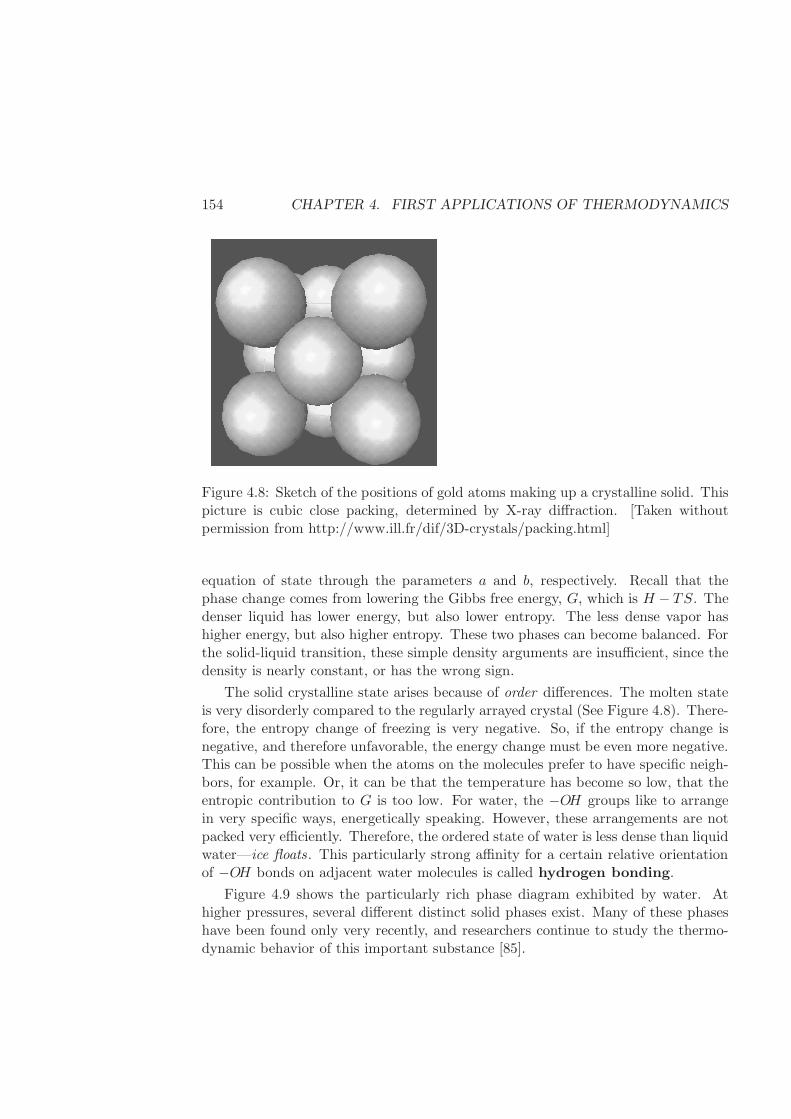
154 CHAPTER 4. FIRST APPLICATIONS OF THERMODYNAMICS
Figure 4.8: Sketch of the positions of gold atoms making up a crystalline solid. Thispicture is cubic close packing, determined by X-ray diffraction. [Taken withoutpermission from http://www.ill.fr/dif/3D-crystals/packing.html]
equation of state through the parameters a and b, respectively. Recall that thephase change comes from lowering the Gibbs free energy, G, which is H − TS. Thedenser liquid has lower energy, but also lower entropy. The less dense vapor hashigher energy, but also higher entropy. These two phases can become balanced. Forthe solid-liquid transition, these simple density arguments are insufficient, since thedensity is nearly constant, or has the wrong sign.
The solid crystalline state arises because of order differences. The molten stateis very disorderly compared to the regularly arrayed crystal (See Figure 4.8). There-fore, the entropy change of freezing is very negative. So, if the entropy change isnegative, and therefore unfavorable, the energy change must be even more negative.This can be possible when the atoms on the molecules prefer to have specific neigh-bors, for example. Or, it can be that the temperature has become so low, that theentropic contribution to G is too low. For water, the −OH groups like to arrangein very specific ways, energetically speaking. However, these arrangements are notpacked very efficiently. Therefore, the ordered state of water is less dense than liquidwater—ice floats. This particularly strong affinity for a certain relative orientationof −OH bonds on adjacent water molecules is called hydrogen bonding.
Figure 4.9 shows the particularly rich phase diagram exhibited by water. Athigher pressures, several different distinct solid phases exist. Many of these phaseshave been found only very recently, and researchers continue to study the thermo-dynamic behavior of this important substance [85].
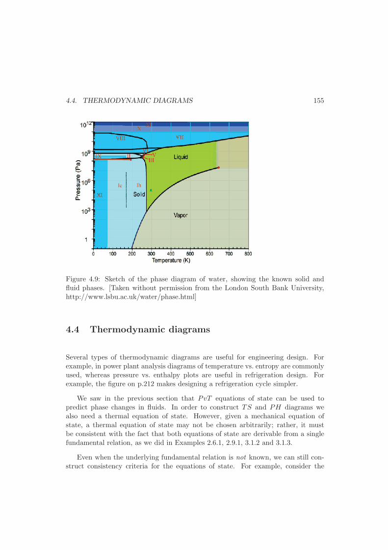
4.4. THERMODYNAMIC DIAGRAMS 155
Figure 4.9: Sketch of the phase diagram of water, showing the known solid andfluid phases. [Taken without permission from the London South Bank University,http://www.lsbu.ac.uk/water/phase.html]
4.4 Thermodynamic diagrams
Several types of thermodynamic diagrams are useful for engineering design. Forexample, in power plant analysis diagrams of temperature vs. entropy are commonlyused, whereas pressure vs. enthalpy plots are useful in refrigeration design. Forexample, the figure on p.212 makes designing a refrigeration cycle simpler.
We saw in the previous section that PvT equations of state can be used topredict phase changes in fluids. In order to construct TS and PH diagrams wealso need a thermal equation of state. However, given a mechanical equation ofstate, a thermal equation of state may not be chosen arbitrarily; rather, it mustbe consistent with the fact that both equations of state are derivable from a singlefundamental relation, as we did in Examples 2.6.1, 2.9.1, 3.1.2 and 3.1.3.
Even when the underlying fundamental relation is not known, we can still con-struct consistency criteria for the equations of state. For example, consider the
156 CHAPTER 4. FIRST APPLICATIONS OF THERMODYNAMICS
Maxwell-like relation that follows from the analytic property of entropy
∂s(u, v)
∂v∂u=
∂s(u, v)
∂u∂v,
(∂
∂v
1
T
)
u
=
(∂
∂u
P
T
)
v
. (4.50)
The second line follows from the alternative definitions for temperature and pressure,Eqs. (2.30) and Eqs. (2.31). If we use the van der Waals equation of state to evaluatethe right side, we obtain
− 1
T 2
(∂T
∂v
)
u
=a
T 2v2
(∂T
∂u
)
v
, van der Waals fluid.
Multiplying each side by T 2 (∂u/∂T )v and using Eqn. (A.20), we obtain
(∂u
∂v
)
T
=a
v2, van der Waals fluid. (4.51)
Note that the right sides of Eqs. (4.50) and (4.51) are determined by the PV Tequation of state, whereas the left sides are determined by a thermal equation ofstate u = u(T, v). This result shows that it is not correct to use a thermal equation ofstate that depends only on temperature with a van der Waals mechanical equation ofstate. Note that we used the PV T relation only, without the fundamental relation,to derive Eqn. (4.51). We now illustrate two different (but equivalent) methods forobtaining thermodynamic diagrams.
4.4.1 Construction of fundamental relations from two equations ofstate for single-component systems
So far we have accepted ‘given’ fundamental relations from which we constructequations of state. However, one typically analyzes experimental data to arriveat an equation of state: pressure measured at several temperatures and volumes,and heat capacity as a function of temperature. The very first example of Chapter2 made exactly such a connection from experiment to equation of state. Here weillustrate how one can construct the fundamental Helmholtz relation from just thesetwo equations of state.4
Say we measure C idealP (T ) and P (T, v) for a range of temperatures and specific
volumes. Then, since our independent variables are T and v, the natural potential is
4The first example of deriving a fundamental relation from equations of state was given for arubber band in §3.7.1.
4.4. THERMODYNAMIC DIAGRAMS 157
Helmholtz potential. Recall that the differential for the Helmholtz potential allowsus to write P = − (∂f/∂v)T . Hence for the van der Waals equation of state we maywrite
(∂f
∂v
)
T
= − RT
v − b+
a
v2. (4.52)
Integrating both sides over specific volume from an ideal reference volume v0 toarbitrary v yields
f(T, v)− f [T, v0] = −RT log
(v − b
v0 − b
)
− a
(1
v− 1
v0
)
. (4.53)
We need to find f [T, v0], which is determined by the thermal equation of state.Recalling that the fluid is an ideal gas at v0, we write
f [T, v0] = f [T0, v0] +
∫ T
T0
(∂f ideal
∂T
)
v
∣∣∣∣v=v0,T=T ′
dT ′
= f0 −∫ T
T0
sideal[T ′, v0]dT′
= f0 −∫ T
T0
s0 +
∫ T ′
T0
(∂sideal
∂T ′′
)
v0
dT ′′
dT ′
= f0 − s0(T − T0)−∫ T
T0
∫ T ′
T0
cidealv [T ′′]T ′′ dT ′′dT ′, (4.54)
where the second line follows from the differential for F , and the fourth line followsfrom the definition of the constant-volume heat capacity. We can simplify the doubleintegral a bit by changing the order of integration
f [T, v0]− f0 + (T − T0)s0 = −∫ T
T0
∫ T ′′
T0
cidealv (T ′)T ′ dT ′dT ′′
= −∫ T
T0
∫ T
T ′
cidealv (T ′)T ′ dT ′′dT ′
= −∫ T
T0
(T − T ′
T ′
)
cidealv (T ′)dT ′. (4.55)
The second line follows from a change in the order of integration, and the third fromperforming the integration over T ′′. We have now found a very convenient form forthe fundamental Helmholtz relation of a general van der Waals fluid
158 CHAPTER 4. FIRST APPLICATIONS OF THERMODYNAMICS
f = f0 − s0(T − T0)−RT log
(v − b
v0 − b
)
− a
(1
v− 1
v0
)
+
∫ T
T0
(T ′ − T
T ′
)
cidealv (T ′)dT ′, general van der Waals fluid. (4.56)
Since v0 is an ideal volume we could further simplify this equation using v0 ≫ band a/v0 makes a negligible contribution to the pressure. We may now constructall possible thermodynamic diagrams for this fluid.
For example, we may find an equation of state for the entropy by taking thederivative of each side of Eqn. (4.56) with respect to T
s(T, v) = s0 +R log
(v − b
v0 − b
)
+
∫ T
T0
cidealv (T ′)T ′ dT ′. (4.57)
Also, the thermal equation of state may be found from the definition of f , Eqn. (3.10)
u(T, v) = f(T, v) + Ts(T, v)
= u0 − a
(1
v− 1
v0
)
+
∫ T
T0
cidealv (T ′)dT ′. (4.58)
It is worth considering the form of Eqn. (4.58). We see that the internal energydepends on both temperature and volume. Only in the ideal limit v = v0 (ora = 0) does the internal energy depend on temperature only. Whenever one usesa volume-independent heat-capacity expression alone to find changes in internalenergy or enthalpy, one is necessarily assuming ideality, and the heat capacity inEqs. (4.58) and (4.56) are ideal heat capacities. If the system is non-ideal, either thefundamental Helmholtz potential should be found, or the appropriate PV T relationshould be used to find the residual properties discussed in §4.4.2.
For a general pressure-explicit equation of state, using the steps above we find
f = f0 − s0(T − T0) +RT
∫ v0
v
z(T, v)
vdv +
∫ T
T0
(T ′ − T
T ′
)
cidealv (T ′)dT ′. (4.59)
Now we see from where many of the fundamental relations in Appendix §B come.Also, using relations derived from statistical mechanics, one can even get cidealv fromIR spectroscopy measurements (see Problem 6.3.C). Alternatively, a calorimeter canbe used.
4.4. THERMODYNAMIC DIAGRAMS 159
Example 4.4.1 Construct a TS diagram using a simple van der Waals fluid.
Solution: If the van der Waals fluid is simple, then cidealv = cR is constant,and Eqn. (4.57) is
s = −(∂f
∂T
)
v
= s0 +R log
[(T
T0
)c (v − b
v0
)]
, simple van der Waals fluid.
(4.60)We may also solve the van der Waals equation of state to obtain an explicitexpression for T = T (P, v)
T =v − b
Rv2(a+ Pv2
). (4.61)
Using Eqs. (4.61) and (4.60), we can plot T as a function of S at fixed P , bychanging v parametrically. For example, on a spreadsheet, we fix the pressurefor a single value of P , and make a column of values for v, between, say 2b and20b. In the second column, we can then calculate values for T using Eqn. (4.61).In the third column, we find values for s using Eqn. (4.60). We can then plotan isobar from the second and third columns.
However, we know from our considerations in §4.2.2, that for P < Pc andsome regions of v, the van der Waals fluid is globally unstable and phase sepa-rates. In these regions, there are liquid and vapor phases that are in equilibriumwith each other; hence, the two phases have the same temperature and pres-sure, but may have different volumes, entropies, enthalpies, etc. Inside thisregion, the fluid no longer obeys the equation of state. Hence, we do not drawthe isobars through this region, but instead connect using tie lines the points ofsaturated vapor in equilibrium with saturated liquid. Therefore, when makingthe columns for sub-critical isobars, we must vary the values for the volumein a more careful way. Namely, we systematically vary the values for v untilv = vliq. At this point, P = P sat. In the next row, we put v = vvap, and againP = P sat. In the following rows we again vary v systematically with valuesgreater than v = vvap. Note that the binodal region is always determined bythe procedure in §4.2, and cannot be found directly from s(T, P ) curves.
If we plot T as a function of s at constant pressure, the curves in Figure 4.10result. 2
The dashed line in Figure 4.10 encloses the vapor-liquid region. The entropyat the critical point is found by evaluating s in Eqn. (4.60) at Tc and vc given inEqs. (4.21) and (4.22).
Similarly, a PH diagram for a van der Waals fluid may also be constructed. Themechanical equation of state for the van der Waals fluid is Eqn. (4.17)
P =RT
v − b− a
v2.
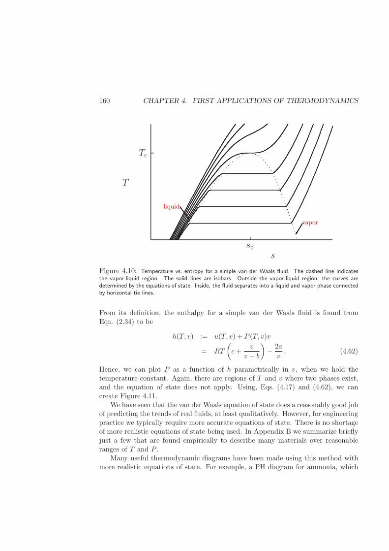
160 CHAPTER 4. FIRST APPLICATIONS OF THERMODYNAMICS
Tc
sc
T
s
vapor
liquid
w
Figure 4.10: Temperature vs. entropy for a simple van der Waals fluid. The dashed line indicatesthe vapor-liquid region. The solid lines are isobars. Outside the vapor-liquid region, the curves aredetermined by the equations of state. Inside, the fluid separates into a liquid and vapor phase connectedby horizontal tie lines.
From its definition, the enthalpy for a simple van der Waals fluid is found fromEqn. (2.34) to be
h(T, v) := u(T, v) + P (T, v)v
= RT
(
c+v
v − b
)
− 2a
v. (4.62)
Hence, we can plot P as a function of h parametrically in v, when we hold thetemperature constant. Again, there are regions of T and v where two phases exist,and the equation of state does not apply. Using, Eqs. (4.17) and (4.62), we cancreate Figure 4.11.
We have seen that the van der Waals equation of state does a reasonably good jobof predicting the trends of real fluids, at least qualitatively. However, for engineeringpractice we typically require more accurate equations of state. There is no shortageof more realistic equations of state being used. In Appendix B we summarize brieflyjust a few that are found empirically to describe many materials over reasonableranges of T and P .
Many useful thermodynamic diagrams have been made using this method withmore realistic equations of state. For example, a PH diagram for ammonia, which
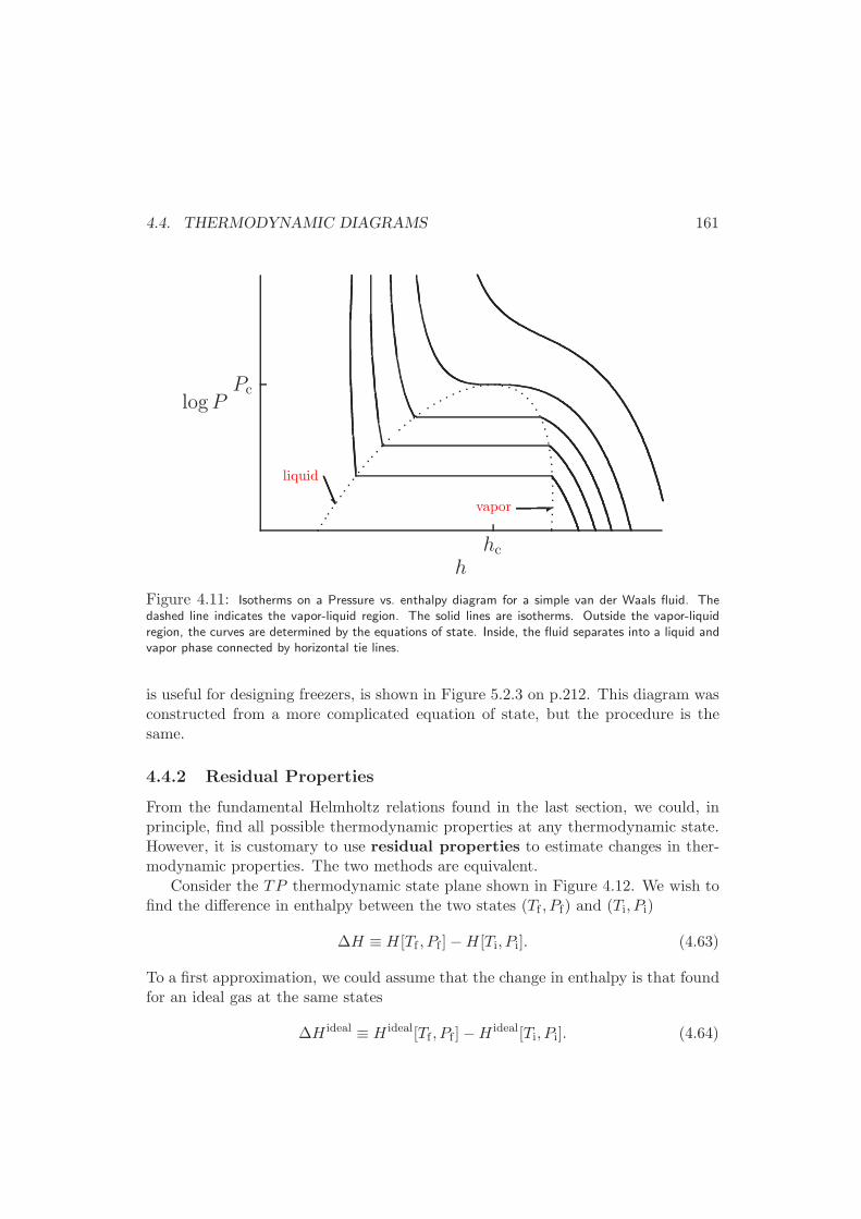
4.4. THERMODYNAMIC DIAGRAMS 161
Pc
hc
logP
h
vapor
liquid
:U
Figure 4.11: Isotherms on a Pressure vs. enthalpy diagram for a simple van der Waals fluid. Thedashed line indicates the vapor-liquid region. The solid lines are isotherms. Outside the vapor-liquidregion, the curves are determined by the equations of state. Inside, the fluid separates into a liquid andvapor phase connected by horizontal tie lines.
is useful for designing freezers, is shown in Figure 5.2.3 on p.212. This diagram wasconstructed from a more complicated equation of state, but the procedure is thesame.
4.4.2 Residual Properties
From the fundamental Helmholtz relations found in the last section, we could, inprinciple, find all possible thermodynamic properties at any thermodynamic state.However, it is customary to use residual properties to estimate changes in ther-modynamic properties. The two methods are equivalent.
Consider the TP thermodynamic state plane shown in Figure 4.12. We wish tofind the difference in enthalpy between the two states (Tf , Pf) and (Ti, Pi)
∆H ≡ H[Tf , Pf ]−H[Ti, Pi]. (4.63)
To a first approximation, we could assume that the change in enthalpy is that foundfor an ideal gas at the same states
∆H ideal ≡ H ideal[Tf , Pf ]−H ideal[Ti, Pi]. (4.64)
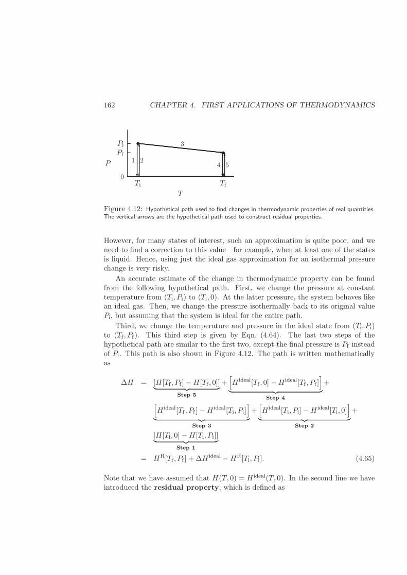
162 CHAPTER 4. FIRST APPLICATIONS OF THERMODYNAMICS
0
Pi
Pf
Ti Tf
P
T
••
1 2
3
4 5
?
6 z
?
6
Figure 4.12: Hypothetical path used to find changes in thermodynamic properties of real quantities.The vertical arrows are the hypothetical path used to construct residual properties.
However, for many states of interest, such an approximation is quite poor, and weneed to find a correction to this value—for example, when at least one of the statesis liquid. Hence, using just the ideal gas approximation for an isothermal pressurechange is very risky.
An accurate estimate of the change in thermodynamic property can be foundfrom the following hypothetical path. First, we change the pressure at constanttemperature from (Ti, Pi) to (Ti, 0). At the latter pressure, the system behaves likean ideal gas. Then, we change the pressure isothermally back to its original valuePi, but assuming that the system is ideal for the entire path.
Third, we change the temperature and pressure in the ideal state from (Ti, Pi)to (Tf , Pf). This third step is given by Eqn. (4.64). The last two steps of thehypothetical path are similar to the first two, except the final pressure is Pf insteadof Pi. This path is also shown in Figure 4.12. The path is written mathematicallyas
∆H = [H[Tf , Pf ]−H[Tf , 0]]︸ ︷︷ ︸
Step 5
+[
H ideal[Tf , 0] −H ideal[Tf , Pf ]]
︸ ︷︷ ︸
Step 4
+
[
H ideal[Tf , Pf ]−H ideal[Ti, Pi]]
︸ ︷︷ ︸
Step 3
+[
H ideal[Ti, Pi]−H ideal[Ti, 0]]
︸ ︷︷ ︸
Step 2
+
[H[Ti, 0]−H[Ti, Pi]]︸ ︷︷ ︸
Step 1
= HR[Tf , Pf ] + ∆H ideal −HR[Ti, Pi]. (4.65)
Note that we have assumed that H(T, 0) = H ideal(T, 0). In the second line we haveintroduced the residual property, which is defined as
4.4. THERMODYNAMIC DIAGRAMS 163
MR(T, P ) :=M(T, P ) −M ideal(T, P ), (4.66)
the difference between the real property M (e.g., H,U, S, F,G) and its value atthe same temperature and pressure if the system were an ideal gas. We see fromEqn. (4.65) that the residual properties are corrections to changes found assumingan ideal gas.
Using the first two steps of the hypothetical path shown in Figure 4.12, we canfind the residual properties from an equation of state. Assume that we are givena volume-explicit PV T equation of state z = z(T, P ), where z := Pv/RT is calledthe compressibility factor. We can find the residual Helmholtz potential fromthe following manipulation
FR(T, P ) := F (T, P )− F ideal(T, P )
= [F (T, P )− F (T, 0)] −[
F ideal(T, P )− F ideal(T, 0)]
=
∫ P
0
[(∂F
∂P
)
T
−(∂F ideal
∂P
)
T
]
dP
= −∫ P
0
[
P
(∂V
∂P
)
T
− P
(∂V ideal
∂P
)
T
]
dP
= −∫ P
0
[
NRT
(∂z
∂P
)
T
− zNRT
P+NRT
P
]
dP
= −NRT (z − 1) +NRT
∫ P
0(z − 1)
dP
P.
We used the differential for F to obtain the fourth line; that V = zNRT/P andV ideal = NRT/P to obtain the fifth; and the fundamental theorem of calculus toobtain the third and sixth lines. If we perform similar manipulations on the otherpotentials and entropy we obtain the following relations.
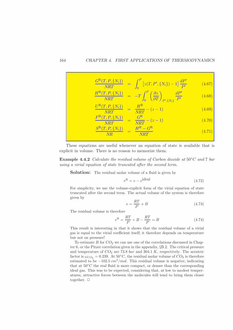
164 CHAPTER 4. FIRST APPLICATIONS OF THERMODYNAMICS
GR(T, P, Ni)NRT
=
∫ P
0
[z(T, P ′, Ni)− 1
] dP ′
P ′ (4.67)
HR(T, P, Ni)NRT
= −T∫ P
0
(∂z
∂T
)
P ′,Ni
dP ′
P ′ (4.68)
UR(T, P, Ni)NRT
=HR
NRT− (z − 1) (4.69)
FR(T, P, Ni)NRT
=GR
NRT− (z − 1) (4.70)
SR(T, P, Ni)NR
=HR −GR
NRT(4.71)
These equations are useful whenever an equation of state is available that isexplicit in volume. There is no reason to memorize them.
Example 4.4.2 Calculate the residual volume of Carbon dioxide at 50C and 7 barusing a virial equation of state truncated after the second term.
Solution: The residual molar volume of a fluid is given by
vR = v − videal (4.72)
For simplicity, we use the volume-explicit form of the virial equation of statetruncated after the second term. The actual volume of the system is thereforegiven by
v =RT
P+B (4.73)
The residual volume is therefore
vR =RT
P+B − RT
P= B (4.74)
This result is interesting in that it shows that the residual volume of a virialgas is equal to the virial coefficient itself; it therefore depends on temperaturebut not on pressure!
To estimate B for CO2 we can use one of the correlations discussed in Chap-ter 6, or the Pitzer correlation given in the appendix, §B.2. The critical pressureand temperature of CO2 are 73.8 bar and 304.1 K, respectively. The acentricfactor is ωCO2 = 0.239. At 50C, the residual molar volume of CO2 is thereforeestimated to be −102.5 cm3/mol. This residual volume is negative, indicatingthat at 50C the real fluid is more compact, or denser than the correspondingideal gas. This was to be expected, considering that, at low to modest temper-atures, attractive forces between the molecules will tend to bring them closertogether. 2
4.4. THERMODYNAMIC DIAGRAMS 165
Example 4.4.3 Find an expression for the residual enthalpy using a pressure-expansion virial equation of state, §B.2.
Solution: The virial equation of state can be written
z(T, P ) = 1 +B′(T )P + C′(T )P 2 + . . . .
We see from Eqn. (4.68) that we need the partial derivative of z with respectto T at constant P . So, if we take the derivative of each side of this equationwith respect to T holding P constant, we obtain
(∂z
∂T
)
P
= PdB′
dT+ P 2 dC
′
dT+ . . . .
Now we multiply each side of this equation by (−T/P ), and integrate over Pfrom 0 to P to obtain
HR
NRT= −T
[
PdB′
dT+P 2
2
dC′
dT+ . . .
]
,
using Eqn. (4.68). 2
Virial expansions are very accurate when restricted to gases that are not verydense. For dense gases or liquids, we typically have available equations of statethat are explicit in pressure, rather than volume. Hence, Eqs. (4.67) through (4.71)cannot be used for these PV T relations. Therefore, we require integrals over volumeinstead of pressure for pressure-explicit equations of state. We can use argumentsanalogous to those above to obtain the appropriate integrals; however, a subtle, butimportant, difference should be noted.
The definition for residual properties, Eqn. (4.66) requires that we find the prop-erty in the ideal state at the same temperature and pressure, not the same volume.Hence, to find the residual Helmholtz potential at a given temperature and volume,we write
FR(T, V ) = F (T, V )− F ideal
(
T,NRT
P (T, V )
)
.
Note that the volume specified for the ideal property is given by NRT/P , and notV . The P in this expression must be found from the nonideal equation of stateP (T, V ). To find these values we integrate from V = ∞ to V , since the systembehaves ideally at infinite volume
FR(T, V ) =
∫ V
∞
(∂F
∂V
)
T
dV −∫ NRT/P
∞
(∂F ideal
∂V
)
T
dV
= −∫ V
∞PdV +
∫ NRT/P
∞P idealdV, constant T .
166 CHAPTER 4. FIRST APPLICATIONS OF THERMODYNAMICS
We used the differential for F to obtain the second line. Now we break up the secondintegral into two pieces.
FR(T, V ) = −∫ V
∞PdV +
∫ V
∞P idealdV +
∫ NRT/P
VP idealdV,
= −∫ V
∞
[
P − P ideal]
dV +
∫ NRT/P
VP idealdV,
= −∫ V
∞
[zNRT
V− NRT
V
]
dV +
∫ NRT/P
V
NRT
VdV
= NRT
∫ ∞
V(z − 1)
dV
V−NRT log z, constant T .
To obtain the third line, we used the ideal gas law and the definition for the com-pressibility factor z. If we perform similar manipulations for other quantities, weobtain the following useful relations.
FR(T, V, Ni)NRT
=
∫ ∞
V
[z(T, V ′, Ni)− 1
] dV ′
V ′ − log z (4.75)
UR(T, V, Ni)NRT
= −T∫ ∞
V
(∂z
∂T
)
V ′,Ni
dV ′
V ′ (4.76)
GR(T, V, Ni)NRT
=FR
NRT+ (z − 1) (4.77)
HR(T, V, Ni)NRT
=UR
NRT+ (z − 1) (4.78)
SR(T, V, Ni)NR
=UR − FR
NRT(4.79)
It is easier to obtain these results by a straightforward change of variable ofintegration for the integrals showing up in Eqs. (4.67 - 4.71). Either way, theseequations should not be memorized.
Example 4.4.4 Find the change in specific residual internal energy predicted by theRedlich-Kwong equation of state for methyl chloride for an initial state P0 = 70bar,T0 = 460K and a final state Pf = 50 bar, and Tf = 450K.
Solution: The Redlich-Kwong equation of state, Eqn. (B.33) can be writtenas
z(T, v) =v
v − b− a
RT 3/2(v + b),
4.4. THERMODYNAMIC DIAGRAMS 167
which is a pressure-explicit PV T relation. Hence, we insert this equation intoEqn. (4.76) to obtain
uR = − 3a
2√T
∫ ∞
v
dv
v(v + b)
=3a
2b√T
log
(v
v + b
)
. (4.80)
To estimate the parameters for the Redlich-Kwong equation of state, we usethe predictions for the critical constants, Eqs. (B.38) and (B.39). For methylchloride, Tc = 416.K, and Pc = 67. bar, according to the NIST ChemistryWebbook. Hence, Eqs. (B.38) and (B.39) yield
a ≈ 159.liter2 · bar ·
√K
mol2= 1.59× 10⁴
liter · J ·√K
mol2
b ≈ 0.0447liter
mol.
We can use these relations to find the residual properties at the beginning andfinal states. The final volume is found by using the formulation for the rootsof a cubic equation, given in the appendix, §A.7. We find that there are singlereal roots, and
vf ≈ 0.566liter
mol.
v0 ≈ 0.363liter
mol.
Inserting these values into Eqn. (4.80) yields
uRf ≈ −1.92kJ
mol.
uR0 ≈ −2.896kJ
mol.
These are the corrections to the ideal internal energy change. We recall fromChapter 2 that the internal energy of an ideal gas depends on temperature only,so we write
∆uideal =
∫ Tf
T0
cidealv [T ]dT
=
∫ Tf
T0
[cidealP [T ]−R
]dT (4.81)
(4.82)
where we used the relation derived earlier, Eqn. (3.85). Especially see the textfollowing this equation. We can find an expression for the constant-pressureideal heat capacity from the NIST Webbook also, which suggests
cidealP = A0 +A1T +A2T2 +A3T
3 +A−2
T 2. (4.83)
168 CHAPTER 4. FIRST APPLICATIONS OF THERMODYNAMICS
where A0 = 3.524690, A1 = 136.9277× 10⁻³, A2 = −82.14196× 10⁻⁶, A3 =20.22797× 10⁻⁹, A−2 = 0.278032× 10⁶ yields the heat capacity in J/(mol K),if the temperature is in Kelvin. If we insert this relation into Eqn. (4.81), wecan integrate to find
∆uideal ≈ −437. J/mol. (4.84)
Therefore, the total internal energy change is
∆u = uRf +∆uideal − uRi (4.85)
≈ 1.42 kJ/mol (4.86)
In other words, we find that the estimate for the change in internal energy isopposite in sign of that predicted for the ideal change alone. 2
It is also possible to create fundamental relations for F or G using residualproperties. See Problems 4.4.L and 4.4.M for more details.
4.5 Summary
In this chapter we introduced the ideas of
• Local stability to show that there are restrictions on values for second-orderderivatives: CP > CV > 0 and κT > κS > 0.
• Global stability to show how a PvT relation can predict boiling and conden-sation of fluids upon heating and cooling.
• Binodal and Spinodal curves. Given any PvT equation of state, the studentshould be able to construct numerically a vapor-liquid phase diagram like thatshown in Figure 4.5.
• Residual properties to generate thermodynamic diagrams, or thermodynamicproperties of real substance. Given a PvT equation of state, the studentshould be able to generate an expression for any residual property. From thisresidual property, and an expression for the ideal heat capacity cidealv (T ), thestudent should also be able to construct any sort of thermodynamic diagram.Examples are TS diagrams, Figure 4.10, or PH diagrams, Figure 4.11.
We also learned how to construct thermodynamic diagrams from fundamentalrelations, or equations of state. In the two-phase region of these diagrams, we usedthe lever rule. As approximations to the binodal curve, we also derived expressionsbased on the Clapeyron equation, such as the Antoine Equation. Alternatives to theAntoine equation have been fit to the PV T equations of state given in Appendix B.
4.5. SUMMARY 169
As examples, we used the van der Waals fluid to predict the vapor-liquid regionof a fluid; we found the chemical potential of water from steam tables; and we usedthe Redlich-Kwong EOS to find energy changes in methyl chloride.
170 CHAPTER 4. FIRST APPLICATIONS OF THERMODYNAMICS
4.6 Exercises
4.1.A: Prove that the local stability criteria on internal energy place restrictions onthe constant-volume heat capacity and the isentropic compressibility, Eqn. (4.11).
4.1.B: Prove that the local stability criteria on F yield restrictions on the isothermalcompressibility, Eqn. (4.13).
4.1.C: Following Example 4.1.2, prove the following stability criterion for the gen-eralized potential
(∂2F
∂T 2
)
V,N
< 0.
4.1.D. Prove the remaining local stability criteria (compared to the above exercise)on the generalized potentials, Eqs. (4.12), in the following way. Begin by noticingthat all of the second order derivatives of the generalized potential can be writtenas first-order derivatives. For example,
(∂2F
∂V 2
)
T
=
(∂
∂V
(∂F
∂V
)
T
)
T
= −(∂P
∂V
)
T
.
Then use Jacobian transformations to write this first-order derivative in terms ofother first-order derivatives that use S and V as independent variables. Finally,replace P and T with their definitions to arrive at second-order derivatives in U , forwhich the local stability criteria are known.
4.1.E. Prove Eqn. (4.15).
4.2.A: Derive the reduced form for the van der Waals equation (4.23) using theexpressions for the critical constants.
4.2.B: A third graphical representation, which is mathematically equivalent to theequal-area rule, Eqn. (4.30), may be found from the Helmholtz potential. The twophases must have equal temperature, but are globally unstable to fluctuations involume. Since it has T and v as canonical independent variables, f is the natu-ral choice for global instability of pure component systems. Figure 4.13 shows theHelmholtz potential at a constant, sub-critical temperature as a function of volumefor the simple van der Waals fluid. We see that there is a portion of the curve that isglobally unstable to volume fluctuations, since it is concave from below. Wheneverthe total volume of the system is constrained to be between vl and vv, the systemcan separate into these two phases, thereby lowering its effective Helmholtz poten-tial to lie on the dashed line connecting these phases. This construction requirescomplete thermodynamic information, whereas our earlier consideration requiredonly an equation of state.
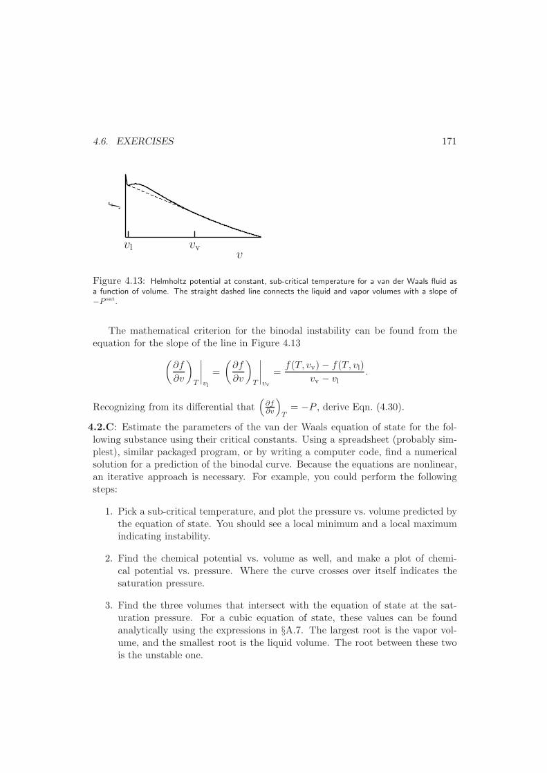
4.6. EXERCISES 171
v
f
vvvl
Figure 4.13: Helmholtz potential at constant, sub-critical temperature for a van der Waals fluid asa function of volume. The straight dashed line connects the liquid and vapor volumes with a slope of−P sat.
The mathematical criterion for the binodal instability can be found from theequation for the slope of the line in Figure 4.13
(∂f
∂v
)
T
∣∣∣∣vl
=
(∂f
∂v
)
T
∣∣∣∣vv
=f(T, vv)− f(T, vl)
vv − vl.
Recognizing from its differential that(∂f∂v
)
T= −P , derive Eqn. (4.30).
4.2.C: Estimate the parameters of the van der Waals equation of state for the fol-lowing substance using their critical constants. Using a spreadsheet (probably sim-plest), similar packaged program, or by writing a computer code, find a numericalsolution for a prediction of the binodal curve. Because the equations are nonlinear,an iterative approach is necessary. For example, you could perform the followingsteps:
1. Pick a sub-critical temperature, and plot the pressure vs. volume predicted bythe equation of state. You should see a local minimum and a local maximumindicating instability.
2. Find the chemical potential vs. volume as well, and make a plot of chemi-cal potential vs. pressure. Where the curve crosses over itself indicates thesaturation pressure.
3. Find the three volumes that intersect with the equation of state at the sat-uration pressure. For a cubic equation of state, these values can be foundanalytically using the expressions in §A.7. The largest root is the vapor vol-ume, and the smallest root is the liquid volume. The root between these twois the unstable one.
172 CHAPTER 4. FIRST APPLICATIONS OF THERMODYNAMICS
4. As a check, calculate the two areas between these two curves, from the equalarea formula, Eqn. (4.30) to verify that this is the correct saturation pressureand volumes. Record the values for temperature, saturation pressure, liquidvolume and vapor volume.
5. Pick a new sub-critical temperature and repeat the procedure. Once you haveseveral values for the saturation pressure and liquid volumes, you can plot theleft side of the binodal curve. The vapor volumes provide the right side, andthese meet at the critical point.
Compare your predictions with the tabulated (experimentally determined) valuesfor the normal boiling points of these fluids.
(a) Nitrogen
(b) Oxygen
(c) Methanol
(d) Carbon monoxide
Check: Your binodal curve should be well approximated in reduced form by the ex-pression:
P sat
Pc=
0.1458
v4r− 0.419
v3r− 0.6203
v2r+
1.9266
vr− 0.0341
4.2.D: Derive an equation for the spinodal curve predicted by the Redlich-Kwongequation of state. Plot the spinodal curve, and several isotherms for reasonablevalues for the parameters. Derive the nonlinear equation that determines the di-mensionless critical volume vc/b, and find an approximate value for it.
Show that
vc/b ≈ 3.84732
Pc ≈ 0.0298944
(a2R
b5
)1/3
Tc ≈ 0.34504( a
Rb
)2/3
and, hence Eqs. (B.38) and (B.39).
4.2.E: Do Problem 4.2.C using a Redlich-Kwong fluid.
Check: Your binodal curve should be well approximated in reduced form by the ex-pression:
P sat
Pc= −0.0133
v4r+
0.3215
v3r− 1.6131
v2r+
2.3194
vr− 0.0152
4.6. EXERCISES 173
4.2.F: Do Problem 4.2.C using a Peng-Robinson fluid.Check: Your binodal curve should be well approximated in reduced form by the ex-pression:
P sat
Pc= −0.0266
v4r+
0.3747
v3r− 1.6451
v2r+
2.3075
vr− 0.0049
over a significant range of vr near the critical point for oxygen.
4.2.G: Do Problem 4.2.D using the Schmidt-Wenzel form of Martin’s generalizedcubic equation of state.
4.2.H: Do Problem 4.2.D using the Peng-Robinson equation of state. Show that
vcb
=[
4 + 2√2]1/3
+[
4− 2√2]1/3
+ 1
Pc ≈ 0.0132366(a0b2
)
Tc ≈ 0.1701444( a0bR
)
.
and, hence, Eqs. (B.49) and (B.50).
4.2.I: Do Problem 4.2.D using the Carnahan-Starling equation of state. Show that
vc/b ∼= 7.66613
Pc∼= 0.00441681
a
b2
Tc ∼= 0.0943287a
bR,
and hence, Eqs. (B.28).
4.2.J: Find the critical point for Martin’s cubic EOS when a = a0√T , β = 2b, and
γ = b.
4.2.K: Do Problem 4.2.C for the Carnahan-Starling equation of state. Note thatthis problem is more difficult than for cubic equations of state, since the EOS is afifth-order polynomial in specific volume. It will be necessary to find all the roots,and determine which are physically reasonable for a given T and P sat. One trick tofind all the roots is to use a standard root finding algorithm (such as that found ina spreadsheet), and use synthetic division to reduce the polynomial to fourth order.Then, the second root can be found by the algorithm, and the procedure is repeated.Check: Your binodal curve should be well approximated in reduced form by the ex-pression:
P sat
Pc=
0.0089
v6r− 0.1102
v5r+
0.4831
v4r− 0.6908
v3r− 0.6825
v2r+
2.0051
vr− 0.0110
over a significant range of vr near the critical point.

174 CHAPTER 4. FIRST APPLICATIONS OF THERMODYNAMICS
4.2.L: Do Problem 4.2.C using the Schmidt-Wenzel form of Martin’s generalizedcubic equations of state for oxygen.Check: Your binodal curve should be well approximated in reduced form by the ex-pression:
P sat
Pc= −0.0970
v4r+
0.9129
v3r− 3.2786
v2r+
4.2369
vr+ 0.0443
over a significant range of vr near the critical point, when you use an acentric factorvalue of 0.487 (ethylene glycol).
4.2.M: Do Problem 4.2.C using the Anderko-Pitzer equation of state for propane.Compare your results to Table B.1. Note that this problem is a little harder thanthe cubic equations, since five roots are possible, and no analytic method exists tofind them. One straightforward way to find all the roots is to first find one rootv1 by iteration (e.g., goal seek in Excel). Then, divide the original polynomial by(v− v1) using synthetic division to find a fourth-order polynomial. Again search fora root to this equation, divide synthetically once more by (v− v2), and then use theanalytic expressions for the resulting cubic equation.
(Hint: It is easiest to perform the entire calculation in reduced form to obtainP satr vs. vr.)
4.2.N: Use the Benedict-Webb-Rubin model to make binodal and spinodal curvesfor one of the fluids listed in Table B.3.
4.2.O. Find an expression for the spinodal curve of the simplified Beattie-Bridgemanmodel
P =RT
v2
[
v +B0
(
1− a
v
)]
− A0
v2
(
1− a
v
)
. (4.87)
4.2.P. The fundamental relation for a fluid suggested by Patel and Teja [97] is
f = f0 − s0(T − T0)−RT log
(v − b
v0
)
+
a(T )
Alog
(2v + b+ c−A
2v + b+ c+A
)
+
∫ T
T0
(T ′ − T
T ′
)
cidealv (T ′)dT ′,
where A :=√b2 + 6bc+ c2, a is a function of temperature, and b and c are constants.
a. Find a PV T equation of state for this fluid.b. Find a U = U(T, V ) equation of state for this fluid.c. Find an expression for κT for this fluid.d. Find P spinodal(v) for this fluid, when a(T ) is assumed constant. Also find an
equation to determine the critical volume, and find a numerical approximation forit. Also determine the critical pressure and temperature.
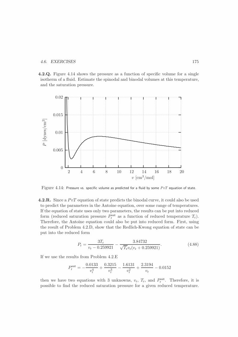
4.6. EXERCISES 175
4.2.Q. Figure 4.14 shows the pressure as a function of specific volume for a singleisotherm of a fluid. Estimate the spinodal and binodal volumes at this temperature,and the saturation pressure.
v [cm3/mol]
P[dynes/cm
2]
2018161412108642
0.02
0.015
0.01
0.005
0
Figure 4.14: Pressure vs. specific volume as predicted for a fluid by some PvT equation of state.
4.2.R. Since a PvT equation of state predicts the binodal curve, it could also be usedto predict the parameters in the Antoine equation, over some range of temperatures.If the equation of state uses only two parameters, the results can be put into reducedform (reduced saturation pressure P sat
r as a function of reduced temperature Tr).Therefore, the Antoine equation could also be put into reduced form. First, usingthe result of Problem 4.2.D, show that the Redlich-Kwong equation of state can beput into the reduced form
Pr =3Tr
vr − 0.259921− 3.84732√
Trvr(vr + 0.259921). (4.88)
If we use the results from Problem 4.2.E
P satr = −0.0133
v4r+
0.3215
v3r− 1.6131
v2r+
2.3194
vr− 0.0152
then we have two equations with 3 unknowns, vr, Tr, and P satr . Therefore, it is
possible to find the reduced saturation pressure for a given reduced temperature.
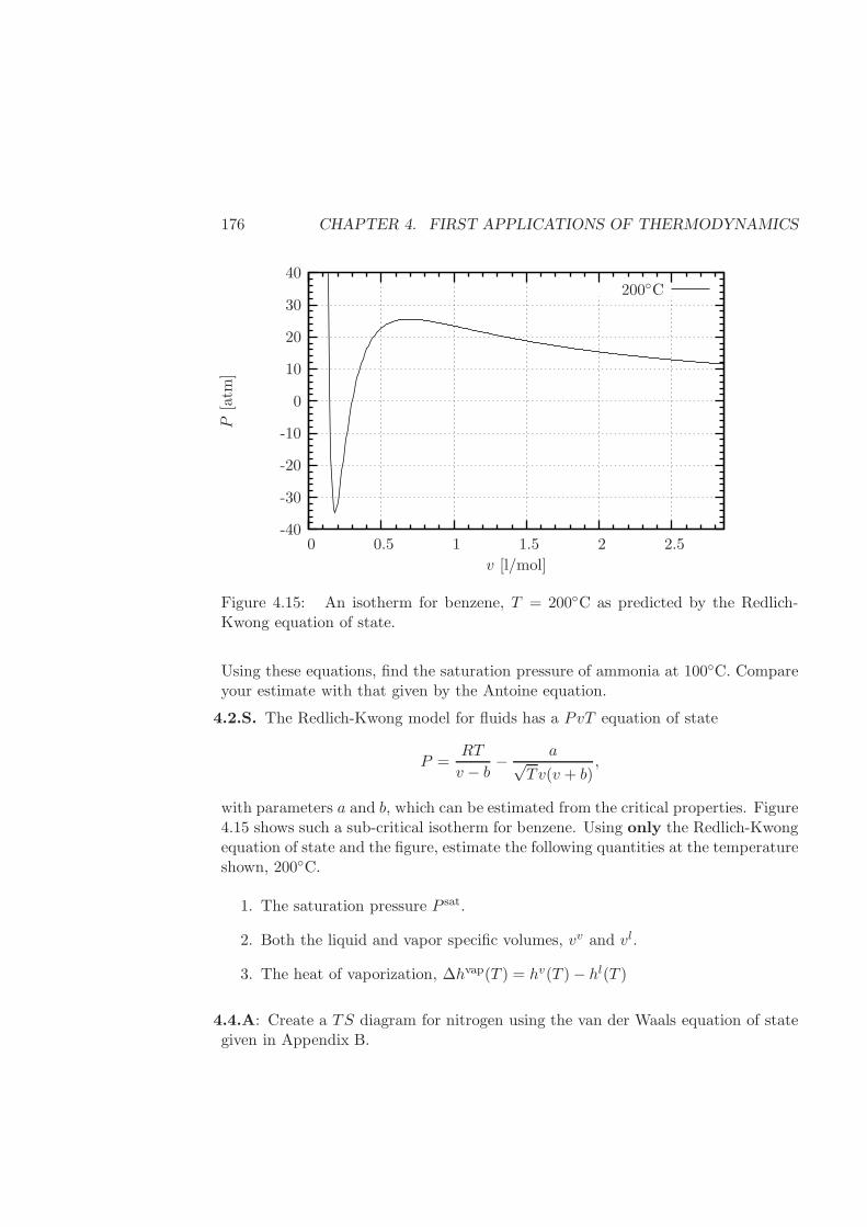
176 CHAPTER 4. FIRST APPLICATIONS OF THERMODYNAMICS
200C
v [l/mol]
P[atm
]
2.521.510.50
40
30
20
10
0
-10
-20
-30
-40
Figure 4.15: An isotherm for benzene, T = 200C as predicted by the Redlich-Kwong equation of state.
Using these equations, find the saturation pressure of ammonia at 100C. Compareyour estimate with that given by the Antoine equation.
4.2.S. The Redlich-Kwong model for fluids has a PvT equation of state
P =RT
v − b− a√
Tv(v + b),
with parameters a and b, which can be estimated from the critical properties. Figure4.15 shows such a sub-critical isotherm for benzene. Using only the Redlich-Kwongequation of state and the figure, estimate the following quantities at the temperatureshown, 200C.
1. The saturation pressure P sat.
2. Both the liquid and vapor specific volumes, vv and vl.
3. The heat of vaporization, ∆hvap(T ) = hv(T )− hl(T )
4.4.A: Create a TS diagram for nitrogen using the van der Waals equation of stategiven in Appendix B.
4.6. EXERCISES 177
4.4.B: Create a PH diagram for nitrogen using the van der Waals equations of stategiven in Appendix B.
4.4.C: We can find a generalization to Eqn. (4.51) that is valid for any equation ofstate z = z(T, v). Insert the relation P = z(T, v)RT/v into Eqn. (4.50) and usemanipulations similar to those used to obtain Eqn. (4.51) to find
(∂u
∂v
)
T
=RT 2
v
(∂z
∂T
)
v
.
Compare this result with Eqn. (4.76) used to find the residual internal energy.
4.4.D: Create a Ts diagram for nitrogen using the Redlich-Kwong equation of stategiven in §B.5.
4.4.E: Create a Ts diagram for nitrogen using the Carnahan-Starling equation ofstate given in §B.4.
4.4.F: Create a Ts diagram for nitrogen using a Peng-Robinson fluid.
4.4.G: Derive Eqs. (4.67) through (4.71).
4.4.H: Derive Eqs. (4.76) through (4.79).
4.4.I: Oxygen at 22 bar, 298K is being pumped along a pipe, and passes through avalve, which causes the pressure to drop to 15 bar. Using the Peng-Robinson model,and assuming that such a throttling process is isenthalpic, find the temperaturedownstream of the valve.
4.4.J: Use the Anderko-Pitzer equation of state to create expressions for the resid-ual properties. Write a spreadsheet or computer program to plot values for thesequantities as functions of reduced temperature, and reduced volume; two plots foreach quantity will be necessary to include the acentric factor (e.g., h = h0(Tr, Pr) +ωh1(Tr, Pr)).
4.4.K: Using the expressions for residual properties, Eqs. (4.67) through (4.71),and its definition, find an expression for CP , given expressions for C ideal
P (T ) andz(T, P, Ni).
4.4.L: It is also possible to use the residual properties to generate fundamental re-lations. For example, pick (T0, P0) as an ideal reference state. Then, we may usean equation similar to (4.65) to find G(T, P,N) − Ng0, where g0 is the specificGibbs potential at the reference state. Find ∆Gideal, and use Eqn. (4.67) to find thefundamental relation for G from cidealv (T ) and z(T, P,N).
4.4.M: Using steps analogous to those in Problem 4.4.L find a fundamental relationF (T, V,N) from cidealv (T ) and z(T, V,N).
178 CHAPTER 4. FIRST APPLICATIONS OF THERMODYNAMICS
4.4.N. Beattie and Bridgeman have an empirical mechanical equation of state withseveral parameters. A simplified version with only 4 parameters is
P =RT
v2
[
v +B0
(
1− a
v
)]
− A0
v2
(
1− a
v
)
, (4.89)
where a, b, A0 and B0 are all constants.Derive a fundamental relation for this fluid.
4.4.O: Estimate the minimum amount of work necessary to pump up my bicycle tiresufficiently slowly so that the process is isothermal, by using the following steps.
1. The tire has a width of 1.5in, and a diameter of 22inch. Estimate the volumeof air in the tire.
2. When full, the tire is at 7bar. Assuming the air is all nitrogen at room tem-perature, use the Peng-Robinson model to estimate the number of moles ofgas in the tire.
3. What is the volume of the air at the same temperature, but at ambient pres-sure?
4. Now calculate the minimum work necessary to compress this air to 7barisothermally. You should remember that isothermal work is equivalent tothe change in a certain thermodynamic quantity.
4.4.P: We here wish to do the same calculation as Problem 4.4.O, except whenthe process is adiabatic instead of isothermal. This calculation is more involved,because reversible, adiabatic compression of the gas is isentropic, not isothermal.Therefore, the final temperature (after pumping adiabatically, but before the tirehas cooled down) is not known. However, we do want the pressure in the tire tobe 7bar at ambient temperature (after the tire has cooled down), so the numberof moles is still the same. Now estimate the final temperature and pressure in thetire assuming adiabatic pumping. Also calculate the minimum total work necessary.Which process requires more work, the adiabatic or the isothermal pumping? Why?
Chapter 5
Application to Process Design:Flow Systems
Young lady, in this house we obey the laws of thermodynamics!
– Homer J. SimpsonTo his daughter Lisa, who has
built a perpetual motion device.
Traditional application of thermodynamics to engineering problems involves pro-cesses that are flowing. For example, an engineer might design a refrigerator in whicha refrigerant is pumped in a continuous cycle through a coil of tubing, or a gener-ator where steam is pumped in a power cycle through several pieces of equipment.Hence, engineering has placed a large emphasis on balances in flowing systems. Suchflow systems involve time as an independent variable. However, thermodynamicsapplies only to equilibrium states, and the introduction of time is strictly forbidden.The study of time-dependent processes actually falls within the domains of transportphenomena, and non-equilibrium thermodynamics.
Whereas the field of transport phenomena is relatively well advanced and wellunderstood, non-equilibrium thermodynamics is a developing field of research, andthe fundamental postulates are by no means agreed upon [64, 7].
We will restrict ourselves here to the simplest of such time-dependent systems.Namely, we will assume that our system is in a local state of equilibrium. Suchan assumption allows us to use the quantities derived for equilibrium systems aslocal variables that depend upon position and time. This simplification is usuallyapplicable whenever the local response time of a system is much more rapid thanthe time scale of the whole process. In this way, we can simplify many engineeringflow problems to equivalent equilibrium thermodynamics problems.
179
180 CHAPTER 5. APPLICATION TO PROCESS DESIGN: FLOW SYSTEMS
For example, consider water flowing through a heat exchanger. If we follow asmall packet of water as it flows through the system, it will experience work throughpressure forces, and heat fluxes from neighboring bits of fluid. The water can respondvery quickly to such changes, and reach equilibrium within one microsecond of achange. The time rate for imposition of such changes is much longer, perhaps neverfaster than one millisecond for our example. Hence, the fluid element “feels” as if itis always in a heat bath at the local temperature and in a pressure bath at the localpressure. Also, it is “unaware” that other fluid elements elsewhere in the exchangerare at different temperatures and pressures.
On the other hand, such an approximation is not valid for a polymer melt flowingthrough a piece of processing equipment. Polymer melts are composed of long chainsthat rearrange by Brownian motion on relatively long time scales, perhaps severalseconds. Hence, as the polymer fluid element travels through the equipment it caneasily be subjected to rapid changes in pressure and temperature to which it cannotquickly respond so that local equilibrium is not recovered .
Also, there are manufacturing processes where reactions take place on surfaces—such as in semiconductor manufacturing. In these reactions, a plasma is createdabove the surface. For example, a plasma may consist of ions and electrons in alow-density, gas-like state subjected to an oscillating electromagnetic field. Becausethe mass of the electrons is so much smaller than that of the ions, the electronsare more strongly affected by the electromagnetic field. Hence, the ions and theelectrons, although occupying the same space, may not be in thermal equilibriumwith one another, and temperature has no meaning in this situation. Assuminglocal equilibrium would be a poor approximation for these two systems.
To derive the governing equations for flow systems rigorously, we will need todraw upon knowledge gleaned from transport phenomena. Unfortunately, the readermay be unfamiliar with this subject. Therefore, we show the details of transportphenomena in Appendix C for the interested reader, and instead go straight to thenecessary macroscopic balances in §5.1, where these equations are first applied. Westrongly recommend, however, that the student skim Appendix C and return to it,when appropriate, during a transport phenomena course. The method of attack toobtain the important equations is outlined in Figure 5.1 on p.185.
We apply these macroscopic balances in §5.1 to single pieces of equipment. Then,in §5.2 we consider power and refrigeration cycles. Note in these problems thatflowing systems are reduced to simpler equilibrium problems of thermodynamics.
5.1. MACROSCOPIC MASS, ENERGY AND ENTROPY BALANCES 181
5.1 Macroscopic Mass, Energy and Entropy Balances
The macroscopic balances useful for industrial applications may be derived fromthe microscopic balances introduced in Appendix C. The details are largely omittedhere, because excellent derivations may be found in transport phenomena textbooks[10, pp.208–210, 456–458], and really belong in that domain. The derivations arenot exceedingly complex, however, and rely only on the Gauss divergence theorem,and a generalization of the Leibniz formula given in §§A.6 and A.5, respectively.
If we integrate the continuity equation, (C.5) over the volume of our system ofinterest, we obtain the macroscopic mass balance
d
dtMtot +∆m = 0 (5.1)
where Mtot is the total mass of the system, m is the mass flow rate of an inlet orexit stream, and
∆(. . .) :=∑
exits
(. . .)−∑
inlets
(. . .) (5.2)
is the difference in values between all the exit and inlet streams.
Similarly, an integration over the volume of interest of the microscopic energybalance, Eqn. (C.14), yields the macroscopic energy balance
d
dtEtot +∆
[h
Mw+
〈|~v|3〉2〈|~v|〉 + φpot
]
m = Q+ Ws (5.3)
where Etot is the sum total of internal, kinetic and potential energy in the volume,〈|~v|〉 is the average velocity of the stream, φpot is the potential energy of the stream(height times gravity), Q is the rate at which heat flows into the volume from outside,and Ws is the rate at which the environment does ‘shaft’ work on the volume throughmoving boundaries.
A few important things to note about this equation are
• It is necessary to make the local equilibrium approximation (to use Eqn. (C.15))in deriving this equation.
• A few minor assumptions have been made: the extra stress ~~τ contributionto work at the inlets and exits is neglected, and the velocity field is in thedirection of the unit normal at the flow streams [8].
• The heat flow Q contains all forms of heat flow, not just conduction [10,Eqn. (18.4–2)]. If the boundaries are impermeable to matter, then conductionis sufficient. However, if part of the boundary of the macroscopic control
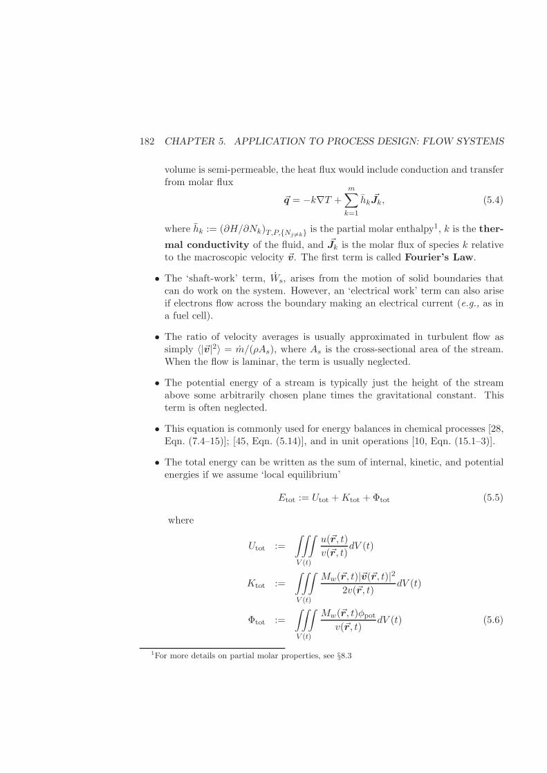
182 CHAPTER 5. APPLICATION TO PROCESS DESIGN: FLOW SYSTEMS
volume is semi-permeable, the heat flux would include conduction and transferfrom molar flux
~q = −k∇T +m∑
k=1
hk ~Jk, (5.4)
where hk := (∂H/∂Nk)T,P,Nj 6=k is the partial molar enthalpy1, k is the ther-
mal conductivity of the fluid, and ~Jk is the molar flux of species k relativeto the macroscopic velocity ~v. The first term is called Fourier’s Law.
• The ‘shaft-work’ term, Ws, arises from the motion of solid boundaries thatcan do work on the system. However, an ‘electrical work’ term can also ariseif electrons flow across the boundary making an electrical current (e.g., as ina fuel cell).
• The ratio of velocity averages is usually approximated in turbulent flow assimply 〈|~v|2〉 = m/(ρAs), where As is the cross-sectional area of the stream.When the flow is laminar, the term is usually neglected.
• The potential energy of a stream is typically just the height of the streamabove some arbitrarily chosen plane times the gravitational constant. Thisterm is often neglected.
• This equation is commonly used for energy balances in chemical processes [28,Eqn. (7.4–15)]; [45, Eqn. (5.14)], and in unit operations [10, Eqn. (15.1–3)].
• The total energy can be written as the sum of internal, kinetic, and potentialenergies if we assume ‘local equilibrium’
Etot := Utot +Ktot +Φtot (5.5)
where
Utot :=
∫∫∫
V (t)
u(~r, t)
v(~r, t)dV (t)
Ktot :=
∫∫∫
V (t)
Mw(~r, t)|~v(~r, t)|22v(~r, t)
dV (t)
Φtot :=
∫∫∫
V (t)
Mw(~r, t)φpotv(~r, t)
dV (t) (5.6)
1For more details on partial molar properties, see §8.3
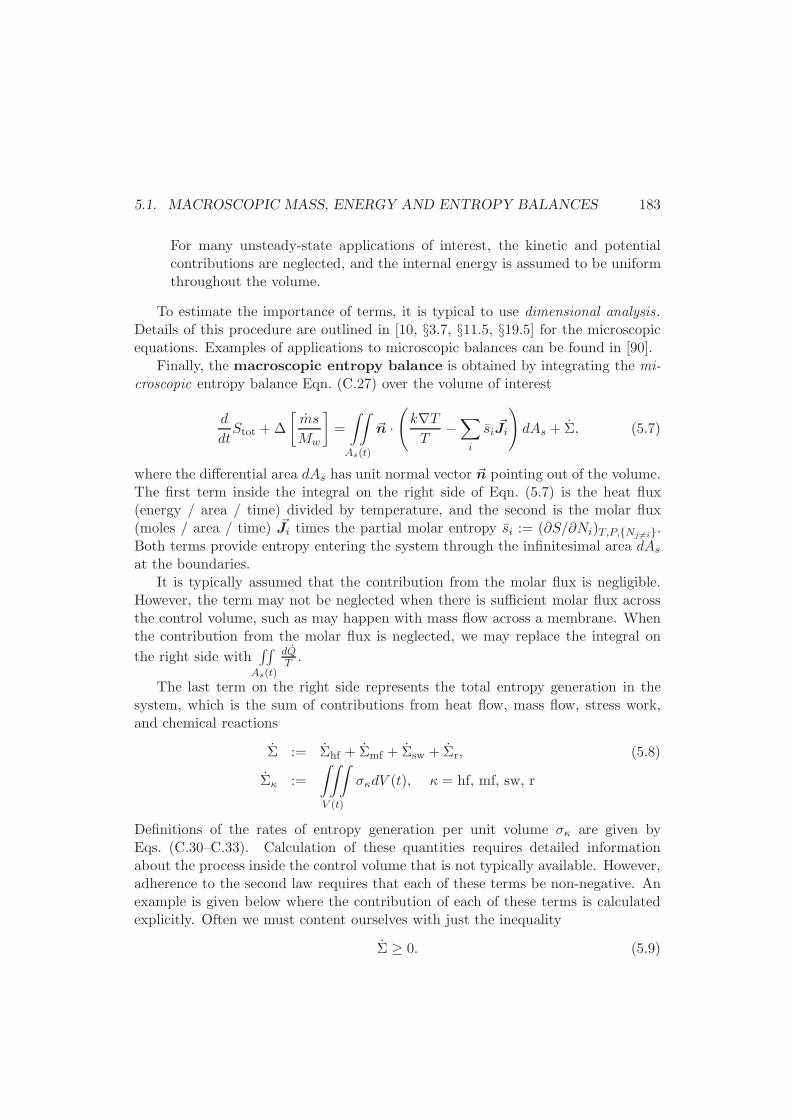
5.1. MACROSCOPIC MASS, ENERGY AND ENTROPY BALANCES 183
For many unsteady-state applications of interest, the kinetic and potentialcontributions are neglected, and the internal energy is assumed to be uniformthroughout the volume.
To estimate the importance of terms, it is typical to use dimensional analysis.Details of this procedure are outlined in [10, §3.7, §11.5, §19.5] for the microscopicequations. Examples of applications to microscopic balances can be found in [90].
Finally, the macroscopic entropy balance is obtained by integrating the mi-croscopic entropy balance Eqn. (C.27) over the volume of interest
d
dtStot +∆
[ms
Mw
]
=
∫∫
As(t)
~n ·(
k∇TT
−∑
i
si ~Ji
)
dAs + Σ, (5.7)
where the differential area dAs has unit normal vector ~n pointing out of the volume.The first term inside the integral on the right side of Eqn. (5.7) is the heat flux(energy / area / time) divided by temperature, and the second is the molar flux(moles / area / time) ~Ji times the partial molar entropy si := (∂S/∂Ni)T,P,Nj 6=i.Both terms provide entropy entering the system through the infinitesimal area dAsat the boundaries.
It is typically assumed that the contribution from the molar flux is negligible.However, the term may not be neglected when there is sufficient molar flux acrossthe control volume, such as may happen with mass flow across a membrane. Whenthe contribution from the molar flux is neglected, we may replace the integral on
the right side with∫∫
As(t)
dQT .
The last term on the right side represents the total entropy generation in thesystem, which is the sum of contributions from heat flow, mass flow, stress work,and chemical reactions
Σ := Σhf + Σmf + Σsw + Σr, (5.8)
Σκ :=
∫∫∫
V (t)
σκdV (t), κ = hf, mf, sw, r
Definitions of the rates of entropy generation per unit volume σκ are given byEqs. (C.30–C.33). Calculation of these quantities requires detailed informationabout the process inside the control volume that is not typically available. However,adherence to the second law requires that each of these terms be non-negative. Anexample is given below where the contribution of each of these terms is calculatedexplicitly. Often we must content ourselves with just the inequality
Σ ≥ 0. (5.9)
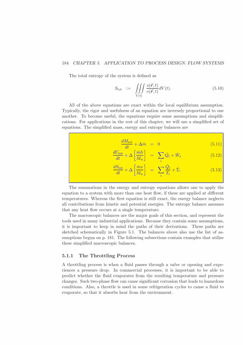
184 CHAPTER 5. APPLICATION TO PROCESS DESIGN: FLOW SYSTEMS
The total entropy of the system is defined as
Stot :=
∫∫∫
V (t)
s(~r, t)
v(~r, t)dV (t). (5.10)
All of the above equations are exact within the local equilibrium assumption.Typically, the rigor and usefulness of an equation are inversely proportional to oneanother. To become useful, the equations require some assumptions and simplifi-cations. For applications in the rest of this chapter, we will use a simplified set ofequations. The simplified mass, energy and entropy balances are
dMtot
dt+∆m = 0 (5.11)
dUtot
dt+∆
[mh
Mw
]
=∑
i
Qi + Ws (5.12)
dStotdt
+∆
[ms
Mw
]
=∑
i
QiTi
+ Σ. (5.13)
The summations in the energy and entropy equations allows one to apply theequation to a system with more than one heat flow, if these are applied at differenttemperatures. Whereas the first equation is still exact, the energy balance neglectsall contributions from kinetic and potential energies. The entropy balance assumesthat any heat flow occurs at a single temperature.
The macroscopic balances are the major goals of this section, and represent thetools used in many industrial applications. Because they contain some assumptions,it is important to keep in mind the paths of their derivations. These paths aresketched schematically in Figure 5.1. The balances above also use the list of as-sumptions begun on p. 181. The following subsections contain examples that utilizethese simplified macroscopic balances.
5.1.1 The Throttling Process
A throttling process is when a fluid passes through a valve or opening and expe-riences a pressure drop. In commercial processes, it is important to be able topredict whether the fluid evaporates from the resulting temperature and pressurechanges. Such two-phase flow can cause significant corrosion that leads to hazardousconditions. Also, a throttle is used in some refrigeration cycles to cause a fluid toevaporate, so that it absorbs heat from the environment.
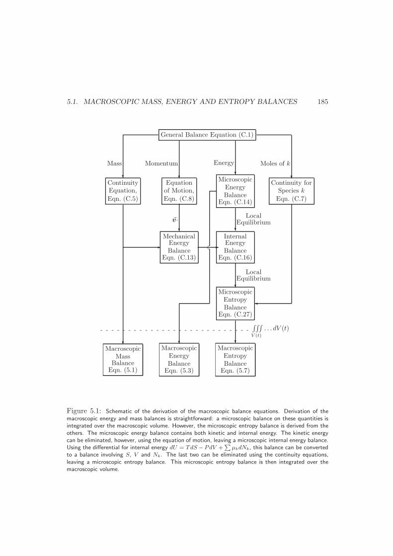
5.1. MACROSCOPIC MASS, ENERGY AND ENTROPY BALANCES 185
General Balance Equation (C.1)
ContinuityEquation,
Eqn. (C.5)
Equationof Motion,Eqn. (C.8)
MicroscopicEnergyBalance
Eqn. (C.14)
Continuity forSpecies k
Eqn. (C.7)
MechanicalEnergyBalance
Eqn. (C.13)
InternalEnergyBalance
Eqn. (C.16)
MicroscopicEntropyBalance
Eqn. (C.27)
MacroscopicMass
BalanceEqn. (5.1)
MacroscopicEnergyBalance
Eqn. (5.3)
MacroscopicEntropyBalanceEqn. (5.7)
?? ??
? ?
?
??
--
?
Mass EnergyMomentum Moles of k
~v· LocalEquilibrium
LocalEquilibrium
- - - - - - - - - - - - - - - - - - - - - - - - - - -∫∫∫
V (t)
. . . dV (t)
Figure 5.1: Schematic of the derivation of the macroscopic balance equations. Derivation of themacroscopic energy and mass balances is straightforward: a microscopic balance on these quantities isintegrated over the macroscopic volume. However, the microscopic entropy balance is derived from theothers. The microscopic energy balance contains both kinetic and internal energy. The kinetic energycan be eliminated, however, using the equation of motion, leaving a microscopic internal energy balance.Using the differential for internal energy dU = TdS −PdV +
∑
µkdNk, this balance can be convertedto a balance involving S, V and Nk. The last two can be eliminated using the continuity equations,leaving a microscopic entropy balance. This microscopic entropy balance is then integrated over themacroscopic volume.
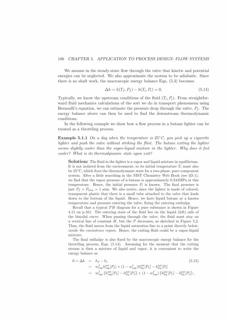
186 CHAPTER 5. APPLICATION TO PROCESS DESIGN: FLOW SYSTEMS
We assume in the steady-state flow through the valve that kinetic and potentialenergies can be neglected. We also approximate the system to be adiabatic. Sincethere is no shaft work, the macroscopic energy balance Eqn. (5.3) becomes
∆h = h(Tf , Pf )− h(Ti, Pi) = 0. (5.14)
Typically, we know the upstream conditions of the fluid (Ti, Pi). From straightfor-ward fluid mechanics calculations of the sort we do in transport phenomena usingBernoulli’s equation, we can estimate the pressure drop through the valve, Pf . Theenergy balance above can then be used to find the downstream thermodynamicconditions.
In the following example we show how a flow process in a butane lighter can betreated as a throttling process.
Example 5.1.1 On a day when the temperature is 25C, you pick up a cigarettelighter and push the valve without striking the flint. The butane exiting the lighterseems slightly cooler than the vapor-liquid mixture in the lighter. Why does it feelcooler? What is its thermodynamic state upon exit?
Solution: The fluid in the lighter is a vapor and liquid mixture in equilibrium.It is not isolated from the environment, so its initial temperature Ti must alsobe 25C, which fixes the thermodynamic state for a two-phase, pure-componentsystem. After a little searching in the NIST Chemistry Web Book (see §D.1),we find that the vapor pressure of n-butane is approximately 0.244MPa at thistemperature. Hence, the initial pressure Pi is known. The final pressure isjust Pf = Patm = 1 atm. We also notice, since the lighter is made of colored,transparent plastic that there is a small tube attached to the valve that leadsdown to the bottom of the liquid. Hence, we have liquid butane at a knowntemperature and pressure entering the valve, fixing the entering enthalpy.
Recall that a typical PH diagram for a pure substance is shown in Figure4.11 on p.161. The entering state of the fluid lies on the liquid (left) side ofthe binodal curve. When passing through the valve, the fluid must stay ona vertical line of constant H , but the P decreases, as sketched in Figure 5.2.Thus, the fluid moves from the liquid saturation line to a point directly below,inside the coexistence region. Hence, the exiting fluid could be a vapor-liquidmixture.
The final enthalpy is also fixed by the macroscopic energy balance for thethrottling process, Eqn. (5.14). Assuming for the moment that the exitingstream is then a mixture of liquid and vapor, it is convenient to write theenergy balance as
0 = ∆h = hf − hi (5.15)
= wfvaphsatvap[Pf ] + (1− wfvap)h
satliq [Pf ]− hsatliq [Pi]
= wfvap(hsatvap[Pf ]− hsatliq [Pi]
)+ (1 − wfvap)
(hsatliq [Pf ]− hsatliq [Pi]
),
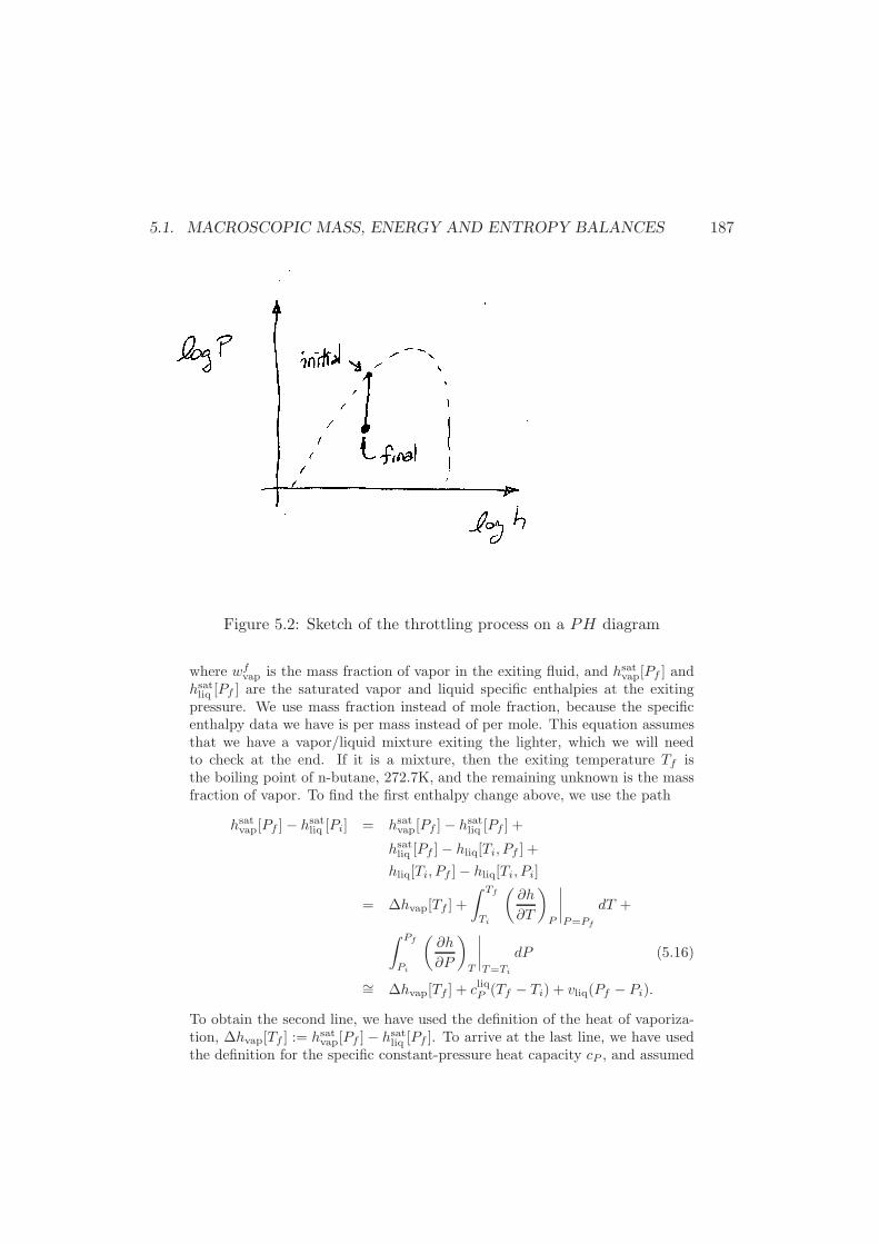
5.1. MACROSCOPIC MASS, ENERGY AND ENTROPY BALANCES 187
Figure 5.2: Sketch of the throttling process on a PH diagram
where wfvap is the mass fraction of vapor in the exiting fluid, and hsatvap[Pf ] andhsatliq [Pf ] are the saturated vapor and liquid specific enthalpies at the exitingpressure. We use mass fraction instead of mole fraction, because the specificenthalpy data we have is per mass instead of per mole. This equation assumesthat we have a vapor/liquid mixture exiting the lighter, which we will needto check at the end. If it is a mixture, then the exiting temperature Tf isthe boiling point of n-butane, 272.7K, and the remaining unknown is the massfraction of vapor. To find the first enthalpy change above, we use the path
hsatvap[Pf ]− hsatliq [Pi] = hsatvap[Pf ]− hsatliq [Pf ] +
hsatliq [Pf ]− hliq[Ti, Pf ] +
hliq[Ti, Pf ]− hliq[Ti, Pi]
= ∆hvap[Tf ] +
∫ Tf
Ti
(∂h
∂T
)
P
∣∣∣∣P=Pf
dT +
∫ Pf
Pi
(∂h
∂P
)
T
∣∣∣∣T=Ti
dP (5.16)
∼= ∆hvap[Tf ] + cliqP (Tf − Ti) + vliq(Pf − Pi).
To obtain the second line, we have used the definition of the heat of vaporiza-tion, ∆hvap[Tf ] := hsatvap[Pf ]− hsatliq [Pf ]. To arrive at the last line, we have usedthe definition for the specific constant-pressure heat capacity cP , and assumed
188 CHAPTER 5. APPLICATION TO PROCESS DESIGN: FLOW SYSTEMS
that it is constant over this small temperature change. We have also used stan-dard thermodynamic manipulations to find that
(∂h∂P
)
T= v−T
(∂v∂T
)
P≈ v, and
assumed that the liquid volume is nearly constant over this pressure change.We could probably obtain a more accurate estimate using residual properties,but this estimate should be sufficiently accurate.
Similarly, we note that
hsatliq [Pf ]− hsatliq [Pi] =
∫ Tf
Ti
(∂h
∂T
)
P
∣∣∣∣P=Pf
dT +
∫ Pf
Pi
(∂h
∂P
)
T
∣∣∣∣T=Ti
dP
≈ cliqP (Tf − Ti) + vliq(Pf − Pi). (5.17)
Putting these expressions into the energy balance yields
0 = wfvap∆hvap[Tf ] + cliqP (Tf − Ti) + vliq(Pf − Pi), (5.18)
from which we can find the mass fraction of butane vapor exiting the lighter,wfvap. After a little more searching on the NIST Chemistry Web Book, we
find that cliqP ≈ 132.4J/mol·K, vliq ≈ 0.01l/mol, and ∆hvap[Tf = 272.7K] =22.44kJ/mol, from which we calculate wfvap ≈ 0.15. Because the mass fractionof vapor is between zero and one, our assumption about a mixture of vapor andliquid is correct.
This is a surprising answer. However, a simple experiment with a lighterand a thermocouple2 verifies that the temperature is at the boiling point ofn-butane at 1 atm. Although there is a greater mass fraction of liquid, thesaturated specific vapor volume is approximately 22l/mol, 2000 times greaterthan the liquid. Hence, the volume fraction of vapor is approximately 0.997,and the liquid is not easily detected. 2
5.1.2 Specifications for a Turbine Generator
A turbine contains blades attached to a shaft that are turned by an expanding gas—something like blowing on the propeller of a model plane, forcing it to turn. It ispossible to estimate the power output from the turbine, and the thermodynamiccondition of the exit stream from the temperature, pressure and mass flow rate ofthe entrance stream, and the exit pressure.
The turbine operates at steady-state, and we neglect kinetic and potential energychanges and approximate the process to be adiabatic. Hence, the macroscopic energybalance Eqn. (5.3) simplifies to
∆ [mh/Mw] = Ws. (5.19)
2Make certain that the liquid butane is entering the tube, and not the vapor.

5.1. MACROSCOPIC MASS, ENERGY AND ENTROPY BALANCES 189
The steady-state mass balance requires that the mass flow rate in and out are equal:min = mout = m. Hence, our energy balance can be written
m (h[Tf , Pf ]/Mw − h[Ti, Pi]/Mw) = Ws. (5.20)
Since we know the entering pressure and temperature, we can use the steam tablesto find the enthalpy of the inlet stream. However, we cannot find the exit enthalpy,because we do not know the exit temperature Tf . Hence, we currently have onlyone equation, but two unknowns: Tf and m.
A second equation is provided by the macroscopic entropy balance Eqn(5.7),which, under our adiabatic approximation and steady-state operation, becomes
∆ [ms/Mw] = Σ. (5.21)
However, here we have introduced a third unknown: Σ, and the situation is notimproved. On the other hand, it is conventional to neglect the entropy generationin the turbine, as a first approximation. Hence, we arrive at the approximationsin = sout. We can then use this relation to find the exit temperature. This lastapproximation, as well as neglected heat losses will make our estimate the maximumpossible power.
Example 5.1.2 Steam is used to drive a turbine. The steam entering the turbine isat a pressure of Pi = 2MPa, and temperature of Ti = 350C, and exits at a pressureof Pf = 30kPa. What flow rate of steam is necessary if the turbine is to provide12MW of power?
Solution: From the steam tables, we find that
h[Ti, Pi]/Mw = 3, 138.6 kJ/kg
s[Ti, Pi]/Mw = 6.9596 kJ/kg·K (5.22)
Again using the steam tables, we seek a temperature that corresponds to a pres-sure of Pf = 30kPa, and a specific entropy of s[Tf , Pf ]/Mw = s[Ti, Pi]/Mw =6.9596kJ/kg ·K. On inspection, we find that this specific entropy lies betweenthe specific entropy of liquid (sliq[30kPa]/Mw = 0.9441kJ/kg·K) and saturatedvapor (svap[30kPa]/Mw = 7.7695kJ/kg · K) at this pressure. Hence, the exitstream must be a mixture of liquid and vapor. If wvap is the mass fraction ofvapor in the exit stream, then we can write
s[Tf , Pf ]/Mw = wvapsvap[Pf ]/Mw + (1 − wvap)sliq[Pf ]/Mw. (5.23)
Solving for the mass fraction, we find wvap ≈ 0.881. We have now completelyspecified the thermodynamic state of the exit stream, and the exit specificenthalpy can be found
h[Tf , Pf ]/Mw = wvaphvap[Pf ]/Mw + (1 − wvap)hliq[Pf ]/Mw
≈ 2, 348.2kJ/kg. (5.24)
190 CHAPTER 5. APPLICATION TO PROCESS DESIGN: FLOW SYSTEMS
We then solve our energy balance equation for the mass flow rate
m =WsMw
∆h≈ 15.2kg/s. (5.25)
This is a very large flow rate of steam. Note that we have made some ratherextreme assumptions to arrive at the answer: no heat loss from the turbine andno entropy generation; we also made a couple of minor assumptions: negligiblekinetic and potential energies.
If we had included entropy generation in the entropy balance, we wouldhave found a higher exit entropy, which would have required a higher exittemperature Tf . The higher exit temperature would, in turn have led to ahigher value for the exit enthalpy, a smaller change in enthalpy ∆h, and alarger mass flow rate would be required to obtain the same shaft work Ws fromthe turbine.
On the other hand, if we had included the effects of heat loss from theturbine, the exiting stream would be predicted to have a decreased entropy,and decreased enthalpy drop. The conventional ad hoc method to account forirreversibility in the turbine is to assume an efficiency factor η, which is the ratioof predicted change in enthalpy divided by the isentropic enthalpy change. 2
5.1.3 Work Requirements for a Pump
Example 5.1.3 Water passes through a pump that raises the pressure from Pi toPf at a mass flow rate of m. Find the rate of work required to operate the pump.
Solution: To a first approximation, we assume that water is incompressible,so that the change in kinetic energy is negligible. We also neglect any changein potential energy. Hence, the energy balance Eqn. (5.3) becomes
∆ [mh/Mw] = Ws. (5.26)
If we neglect entropy and heat fluxes at the boundaries of the pump, then thesystem is isentropic, and we can manipulate the above equation in the followingmanner
Ws =
(m
Mw
)
(∆h)s
=
(m
Mw
)∫ Pf
Pi
(∂h
∂P
)
s
dP
=
(m
Mw
)∫ Pf
Pi
vdP
≈(m
Mw
)
v(Pf − Pi). (5.27)
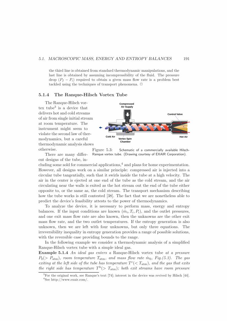
5.1. MACROSCOPIC MASS, ENERGY AND ENTROPY BALANCES 191
the third line is obtained from standard thermodynamic manipulations, and thelast line is obtained by assuming incompressibility of the fluid. The pressuredrop (Pf − Pi) required to obtain a given mass flow rate is a problem besttackled using the techniques of transport phenomena. 2
5.1.4 The Ranque-Hilsch Vortex Tube
The Ranque-Hilsch vor- Compressed Air Supply
Cold AirVortex Spin
Chamber
Control Valve
Hot Air
Figure 5.3: Schematic of a commercially available Hilsch-Ranque vortex tube. (Drawing courtesy of EXAIR Corporation).
tex tube3 is a device thatdelivers hot and cold streamsof air from single initial streamat room temperature. Theinstrument might seem toviolate the second law of ther-modynamics, but a carefulthermodynamic analysis showsotherwise.
There are many differ-ent designs of the tube, in-cluding some sold for commercial applications,4 and plans for home experimentation.However, all designs work on a similar principle: compressed air is injected into acircular tube tangentially, such that it swirls inside the tube at a high velocity. Theair in the center is ejected at one end of the tube as the cold stream, and the aircirculating near the walls is exited as the hot stream out the end of the tube eitheropposite to, or the same as, the cold stream. The transport mechanism describinghow the tube works is still contested [38]. The fact that we are nonetheless able topredict the device’s feasibility attests to the power of thermodynamics.
To analyze the device, it is necessary to perform mass, energy and entropybalances. If the input conditions are known (mi, Ti, Pi), and the outlet pressures,and one exit mass flow rate are also known, then the unknowns are the other exitmass flow rate, and the two outlet temperatures. If the entropy generation is alsounknown, then we are left with four unknowns, but only three equations. Theirreversibility inequality in entropy generation provides a range of possible solutions,with the reversible case providing bounds to the range.
In the following example we consider a thermodynamic analysis of a simplifiedRanque-Hilsch vortex tube with a simple ideal gas.Example 5.1.4 An ideal gas enters a Ranque-Hilsch vortex tube at a pressureP0(> Patm), room temperature Tatm, and mass flow rate m0, Fig.(5.3). The gasexiting at the left side of the tube has temperature T c(< Tatm), and the gas that exitsthe right side has temperature T h(> Tatm); both exit streams have room pressure
3For the original work, see Ranque’s text [74]; interest in the device was revived by Hilsch [44].4See http://www.exair.com/.
192 CHAPTER 5. APPLICATION TO PROCESS DESIGN: FLOW SYSTEMS
Patm, and the same mass flow rate m. What is the maximum possible temperaturedifference between the two exiting streams ∆Tmax = T hmax − T cmin? Why does thevortex tube not violate the second law of thermodynamics?
Solution: A mass balance on the vortex tube tells us that the mass flow rateof each exit stream is one-half that of the inlet: 1
2m0 = mc = mh ≡ m.To a first approximation, we can assume that the changes in kinetic and
potential energy are negligible, and that the vortex tube is adiabatic. Hence,the steady-state energy balance is written
0 = ∆(mh)
= h[T h, Patm]mh + h[T c, Patm]m
c − h[Tatm, P0]m0
=(h[T h, Patm] + h[T c, Patm]− 2h[Tatm, P0]
)m. (5.28)
We used the results from the mass balance to obtain the last line. If we hadan equation of state for h(T, P ), we would now have one equation, but twounknowns: T c and T h. Hence, we need another equation, which is provided bythe entropy balance. Again neglecting entropy fluxes at the solid boundariesfrom heat flows, we obtain for the steady-state entropy balance
s[T h, Patm] + s[T c, Patm]− 2s[Tatm, P0] =Σ
m. (5.29)
Our second equation has introduced another unknown Σ, whose estimationrequires detailed information about the fluid inside the vortex tube. Since wedo not have this detailed information, it might appear that the situation is notimproved. However, we do know from the second law of thermodynamics that
Σ ≥ 0. (5.30)
We are able to calculate the reversible case Σ = 0 as a limit. For the moment,let us keep the term around, and remember that its value must be non-negative.
We can now introduce the necessary equations of state for the ideal gas. Ifwe also assume that the gas is simple, then
h = u+ Pv = cRT +RT = (c+ 1)RT, simple ideal gas, (5.31)
and the energy balance (5.28) becomes
2Tatm = T h + T c. (5.32)
The fundamental entropy relation for a simple ideal gas is given in Chapter 2,Eqn. (2.39)
s = s0 +R log
[(u
u0
)c (v
v0
)]
simple ideal gas. (5.33)
5.1. MACROSCOPIC MASS, ENERGY AND ENTROPY BALANCES 193
We may find the more useful equation of state s = s(T, P ) from this fundamen-tal relation using the equations of state u = cRT and Pv = RT
s = s0 +R log
[(cRT
u0
)c (RT
Pv0
)]
simple ideal gas. (5.34)
Using this equation of state in the entropy balance Eqn. (5.29) yields, after alittle algebraic manipulation,
log
[(T hT c
T 2atm
)c+1(P0
Patm
)2]
=Σ
mR, (5.35)
If we use the result from our energy balance, Eqn. (5.32), to eliminate T c fromthis equation, we find that
0 =
(T h
Tatm
)2
− 2
(T h
Tatm
)
+
(Patm
P0
)2/(c+1)
exp
[
Σ
(c+ 1)mR
]
. (5.36)
This is a quadratic equation in T h/Tatm with two roots. One of the roots givesT h less than Tatm, which is clearly the cold stream. Hence, we find
T h
Tatm= 1 +
√√√√1− (Patm/P0)
2/(c+1)exp
[
Σ
(c+ 1)mR
]
. (5.37)
There are two interesting things to note from this solution. First, since theentropy generation term Σ must be positive, we see that the maximum valuethat can be reached by the hot stream is when Σ = 0. Therefore,
T hmax = Tatm
[
1 +
√
1− (Patm/P0)2/(c+1)
]
. (5.38)
The temperature of the cold stream can be found from this relation and Eqn. (5.32).Thus, we find the maximum temperature difference predicted by a simple idealgas with no entropy generation is
∆Tmax = 2Tatm
√
1− (Patm/P0)2/(c+1)
. (5.39)
If P0∼= 2atm, and c = 5/2 (appropriate for a diatomic gas, like nitrogen, at
sufficiently high temperatures), then this expression gives ∆Tmax/Tatm ∼= 1.14.For Tatm ∼= 298K, this gives a cold stream of 128K!
The second observation about Eqn. (5.37) is that for the solution to be real,the radical must be positive. Therefore, there is a maximum possible entropygeneration
Σmax = 2mR log
(P0
Patm
)
. (5.40)
194 CHAPTER 5. APPLICATION TO PROCESS DESIGN: FLOW SYSTEMS
This limit in entropy generation exists because we have already specified theentrance and exit pressures. When the entropy generation is at a maximum,the radical in Equation (5.37) is zero, and both exit streams have the sametemperature as the inlet stream, Tatm.
Note that throughout the development we have kept careful track of entropygeneration. Yet, we find that it is possible to generate a stream of hot airand a stream of cold air from a stream at room temperature. This soundslike we are getting “something for nothing,” which may violate our intuitionabout the second law of thermodynamics. However, the vortex tube exploitsthe fact that a gas at high pressure has lower entropy than the same gas at lowpressure. Since a pressure drop is required to drive the gas through the system,the entropy of the gas rises. The vortex tube exploits this rise in entropy todrive the process of temperature separation, and the second law is not violated.2
Real vortex tubes are more complicated than this analysis suggests. First, themass flow rate is not necessarily split evenly between the cold and hot exit streams.Secondly, there can be substantial friction losses in the tube, leading to large entropygeneration. Perhaps most importantly, the velocity of the inlet stream is extremelylarge, even near the speed of sound [38]. Therefore, not only should kinetic energy betaken into account, the assumption of local equilibrium may not be valid, violatingthe derivation of the macroscopic balances, Eqs. (5.3) and (5.7).
5.1.5 Fuel Cells
In Examples 3.5.3 and 3.5.4 we did a closed-system analysis of a fuel cell. To performthe analysis we somewhat artificially considered the reactants and products as partof the system. We return here to the fuel cell, but now as an open system in whichreactants flow in, products (and unreacted reactants) flow out, and electrical workis produced. Depending upon the entropy of reaction, heat may flow in or out ofthe cell.
We first perform an energy balance on the cell using Eqn. (5.3). If we assumesteady state and neglect kinetic and potential energy we obtain
∆
[hm
Mw
]
= Q+ Welec. (5.41)
We have also assumed here that the general shaft work can be replaced by a term forelectrical work. If the fuel cell operates isothermally, then the unreacted reactantsdo not contribute to the term on the left side, because their enthalpy is unchanged.Hence, m→ mrxn is the mass flow rate of products in the exit stream, and only thereacted reactants at the entrance side. We neglect the mass of the electrons in theflow.
5.1. MACROSCOPIC MASS, ENERGY AND ENTROPY BALANCES 195
If the temperature and pressure of the fuel cell are known, then the left sidecan be found. In order to find the available electrical work, the heat flow must beknown, which we find from the open entropy balance. Again assuming steady stateand isothermal conditions, and neglecting any molar flux not in the entrance andexit streams simplifies Eqn. (5.7) to
∆
[mrxns
Mw
]
=Q
T+ Σ. (5.42)
We find that the heat flow into the system is
Q = mrxnT∆srxnMw
− T Σ. (5.43)
If the cell operates reversibly (Σ = 0), then this result is the same as that obtainedfor the closed system. Namely, the heat into (or out of) the fuel cell dependson the sign of ∆Srxn. If ∆Srxn < 0, then heat necessarily flows out of the cell.Otherwise, heat is required to enter the cell to maintain isothermal conditions. Anyirreversibility in the operation (arising from temperature gradients, resistance, etc.)mitigates the amount of necessary added heat.
If we insert Q from Eqn. (5.43) into Eqn. (5.41), we obtain
Welec = ∆
[∆grxnmrxn
Mw
]
+ T Σ. (5.44)
Hence, for reversible operation, we get the same result as found in the closedanalysis—the available work is minus the Gibbs free energy of reaction. If theentropy of reaction is positive, an additional cost is incurred from keeping the fuelcell heated, according to Eqn. (5.43). For negative entropy of reaction, no heatingwas necessary, and the maximum work available is when no entropy is generated,Σ = 0. Therefore, we get from Eqn. (5.47)
Wmaxelec = ∆
[∆grxnmrxn
Mw
]
, ∆Srxn < 0. (5.45)
On the other hand, if the entropy of reaction is positive, irreversibility mitigatesthe need for external heating, as we see from Eqn. (5.43). In our earlier, closed-system analysis, we used combustion to heat the cell and finish the analysis. Herewe assume that irreversibility completely obviates the need for heating to obtainthe same result. If no heating is necessary, then Eqn. (5.43) says that the entropygeneration must be
T Σ =mrxnT∆srxn
Mw, ∆Srxn > 0. (5.46)
196 CHAPTER 5. APPLICATION TO PROCESS DESIGN: FLOW SYSTEMS
Then, the maximum electrical work available according to Eqn. (5.47) is
Wmaxelec = ∆
[∆hrxnmrxn
Mw
]
, ∆Srxn > 0. (5.47)
Although the analysis was a little different, these are completely analogous to theresults found for a closed system.
Some operations of the fuel cell leave some fraction of the reactants unreacted.However, the rate of reaction can be found from measuring the electric currentproduced, and knowledge of the number of electrons exchanged in the reaction. Ifthe rate of reaction is Rrxn, then we can write
Rrxn =i
NeF, (5.48)
where i is the current, Ne is the number of electrons transferred in the reaction, andF = NAe = 9.6492 × 10⁴ C/mol = 23060 cal/(mol·eV) = 2.8025 × 10¹⁴ esu/mol isFaraday’s constant, and e is the electron charge. Here C is a Coulomb, esu is anelectrostatic unit, and eV is an electron volt.
Therefore, from data for the current and power (or, equivalently, voltage), wecan find the efficiency of a fuel cell, defined as
η :=Welec
W theoreticalelec
, (5.49)
from the measured electrical work.
Example 5.1.5 The overall reaction in the direct methanol fuel cell is
CH3OH +3
2O2 → CO2 +H2O
The redox reaction that corresponds to methanol oxidation at the fuel cell anode is[3]
CH3OH +H2O → CO2 + 6H+ + 6e−
A direct methanol fuel cell is operated at ambient pressure and 110C. The methanolconcentration is 1M and the flow rate is 360ml/min. The electrode has a geometricsurface area of 225cm2. The average cell performance is given in Table 5.1. What isthe efficiency of the direct methanol fuel cell described above as a function of currentdensity?
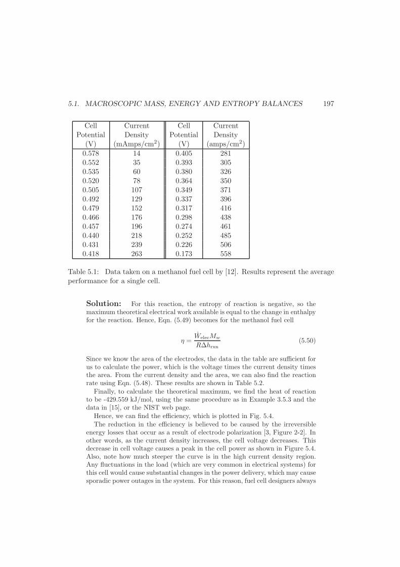
5.1. MACROSCOPIC MASS, ENERGY AND ENTROPY BALANCES 197
Cell Current Cell CurrentPotential Density Potential Density
(V) (mAmps/cm2) (V) (amps/cm2)
0.578 14 0.405 2810.552 35 0.393 3050.535 60 0.380 3260.520 78 0.364 3500.505 107 0.349 3710.492 129 0.337 3960.479 152 0.317 4160.466 176 0.298 4380.457 196 0.274 4610.440 218 0.252 4850.431 239 0.226 5060.418 263 0.173 558
Table 5.1: Data taken on a methanol fuel cell by [12]. Results represent the averageperformance for a single cell.
Solution: For this reaction, the entropy of reaction is negative, so themaximum theoretical electrical work available is equal to the change in enthalpyfor the reaction. Hence, Eqn. (5.49) becomes for the methanol fuel cell
η =WelecMw
R∆hrxn(5.50)
Since we know the area of the electrodes, the data in the table are sufficient forus to calculate the power, which is the voltage times the current density timesthe area. From the current density and the area, we can also find the reactionrate using Eqn. (5.48). These results are shown in Table 5.2.
Finally, to calculate the theoretical maximum, we find the heat of reactionto be -429.559 kJ/mol, using the same procedure as in Example 3.5.3 and thedata in [15], or the NIST web page.
Hence, we can find the efficiency, which is plotted in Fig. 5.4.The reduction in the efficiency is believed to be caused by the irreversible
energy losses that occur as a result of electrode polarization [3, Figure 2-2]. Inother words, as the current density increases, the cell voltage decreases. Thisdecrease in cell voltage causes a peak in the cell power as shown in Figure 5.4.Also, note how much steeper the curve is in the high current density region.Any fluctuations in the load (which are very common in electrical systems) forthis cell would cause substantial changes in the power delivery, which may causesporadic power outages in the system. For this reason, fuel cell designers always
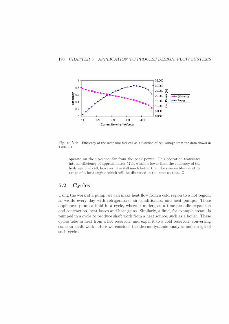
198 CHAPTER 5. APPLICATION TO PROCESS DESIGN: FLOW SYSTEMS
Figure 5.4: Efficiency of the methanol fuel cell as a function of cell voltage from the data shown inTable 5.1.
operate on the up-slope, far from the peak power. This operation translatesinto an efficiency of approximately 57%, which is lower than the efficiency of thehydrogen fuel cell; however, it is still much better than the reasonable operatingrange of a heat engine which will be discussed in the next section. 2
5.2 Cycles
Using the work of a pump, we can make heat flow from a cold region to a hot region,as we do every day with refrigerators, air conditioners, and heat pumps. Theseappliances pump a fluid in a cycle, where it undergoes a time-periodic expansionand contraction, heat losses and heat gains. Similarly, a fluid, for example steam, ispumped in a cycle to produce shaft work from a heat source, such as a boiler. Thesecycles take in heat from a hot reservoir, and expel it to a cold reservoir, convertingsome to shaft work. Here we consider the thermodynamic analysis and design ofsuch cycles.
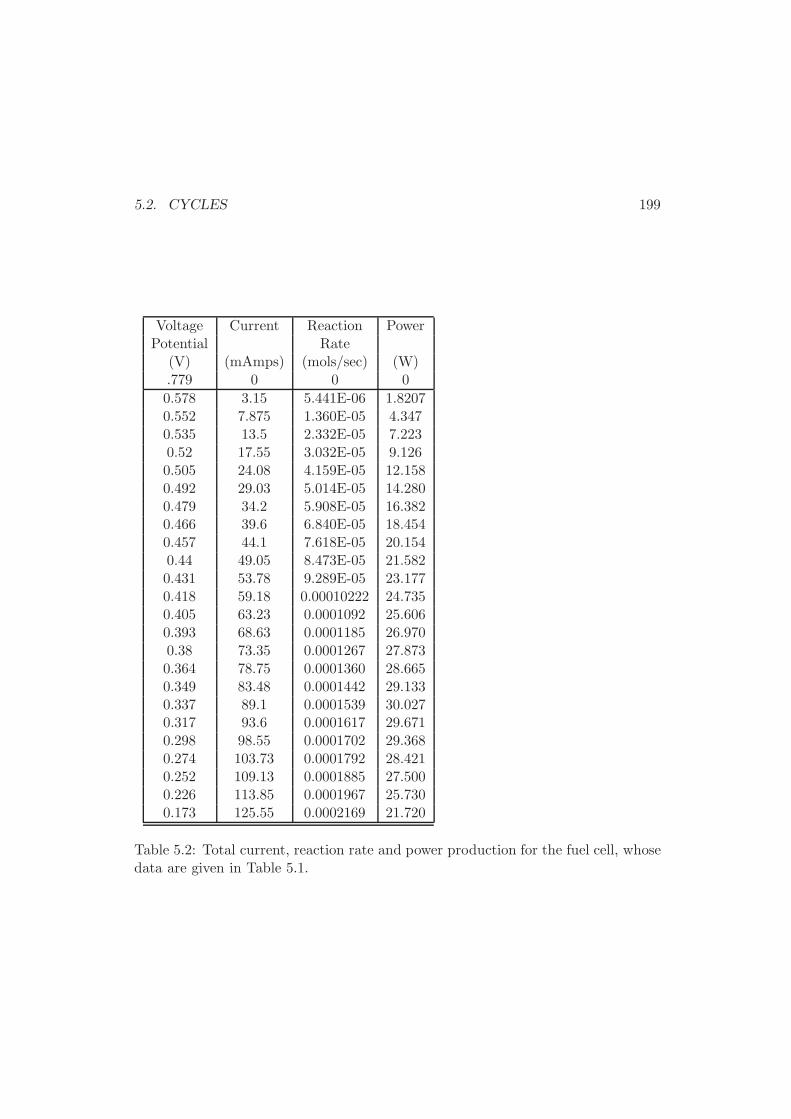
5.2. CYCLES 199
Voltage Current Reaction PowerPotential Rate
(V) (mAmps) (mols/sec) (W).779 0 0 0
0.578 3.15 5.441E-06 1.82070.552 7.875 1.360E-05 4.3470.535 13.5 2.332E-05 7.2230.52 17.55 3.032E-05 9.1260.505 24.08 4.159E-05 12.1580.492 29.03 5.014E-05 14.2800.479 34.2 5.908E-05 16.3820.466 39.6 6.840E-05 18.4540.457 44.1 7.618E-05 20.1540.44 49.05 8.473E-05 21.5820.431 53.78 9.289E-05 23.1770.418 59.18 0.00010222 24.7350.405 63.23 0.0001092 25.6060.393 68.63 0.0001185 26.9700.38 73.35 0.0001267 27.8730.364 78.75 0.0001360 28.6650.349 83.48 0.0001442 29.1330.337 89.1 0.0001539 30.0270.317 93.6 0.0001617 29.6710.298 98.55 0.0001702 29.3680.274 103.73 0.0001792 28.4210.252 109.13 0.0001885 27.5000.226 113.85 0.0001967 25.7300.173 125.55 0.0002169 21.720
Table 5.2: Total current, reaction rate and power production for the fuel cell, whosedata are given in Table 5.1.
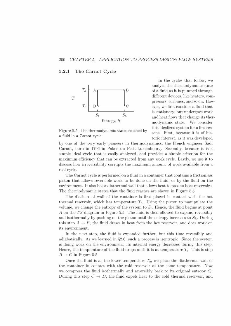
200 CHAPTER 5. APPLICATION TO PROCESS DESIGN: FLOW SYSTEMS
5.2.1 The Carnot Cycle
In the cycles that follow, we
Tc
Th
Sl Sh
T
Entropy, S
A B
CD
-
?
6
Figure 5.5: The thermodynamic states reached by
a fluid in a Carnot cycle.
analyze the thermodynamic stateof a fluid as it is pumped throughdifferent devices, like heaters, com-pressors, turbines, and so on. How-ever, we first consider a fluid thatis stationary, but undergoes workand heat flows that change its ther-modynamic state. We considerthis idealized system for a few rea-sons. First, because it is of his-toric interest, as it was developed
by one of the very early pioneers in thermodynamics, the French engineer SadiCarnot, born in 1796 in Palais du Petit-Luxembourg. Secondly, because it is asimple ideal cycle that is easily analyzed, and provides a simple criterion for themaximum efficiency that can be extracted from any work cycle. Lastly, we use it todiscuss how irreversibility corrupts the maximum amount of work available from areal cycle.
The Carnot cycle is performed on a fluid in a container that contains a frictionlesspiston that allows reversible work to be done on the fluid, or by the fluid on theenvironment. It also has a diathermal wall that allows heat to pass to heat reservoirs.The thermodynamic states that the fluid reaches are shown in Figure 5.5.
The diathermal wall of the container is first placed in contact with the hotthermal reservoir, which has temperature Th. Using the piston to manipulate thevolume, we change the entropy of the system to Sl. Hence, the fluid begins at pointA on the TS diagram in Figure 5.5. The fluid is then allowed to expand reversiblyand isothermally by pushing on the piston until the entropy increases to Sh. Duringthis step A → B, the fluid draws in heat from the hot reservoir, and does work onits environment.
In the next step, the fluid is expanded further, but this time reversibly andadiabatically. As we learned in §2.6, such a process is isentropic. Since the systemis doing work on the environment, its internal energy decreases during this step.Hence, the temperature of the fluid drops until it is at temperature Tc. This is stepB → C in Figure 5.5.
Once the fluid is at the lower temperature Tc, we place the diathermal wall ofthe container in contact with the cold reservoir at the same temperature. Nowwe compress the fluid isothermally and reversibly back to its original entropy Sl.During this step C → D, the fluid expels heat to the cold thermal reservoir, and
5.2. CYCLES 201
requires that we do work.To complete the cycle, the fluid is compressed adiabatically and reversibly back
to its initial state A. Summarizing, we find that the fluid delivers work during stepsA→ B and B → C, and requires work during C → D and D → A; it takes in heatduring step A→ B, and expels heat during C → D.
We can find the total work delivered (delivered − required) from an energybalance on the fluid following all four steps. Since the fluid ends at the same ther-modynamic state where it started, its total change in internal energy is zero. Anenergy balance says that the total heat delivered to the fluid must equal the totalwork delivered. During the isothermal steps, we may write
dU = dU
dQrev + dWrev = TdS − PdV
dQrev = TdS, (5.51)
where we used the definition of heat (2.1) and the differential for U (2.27) to obtainthe second line, and the fact that dWrev = −PdV to obtain the third. If we integratethis equation over the two isothermal steps in the cycle, we obtain
QAB = Th∆S, QCD = −Tc∆S, (5.52)
where ∆S := Sh − Sl. Hence, the total work (−W ) delivered by the fluid to itsenvironment is −W = QAB+QCD = (Th−Tc)∆S, which is just the area of the boxABCD. The coefficient of performance εp is defined as the total work delivereddivided by the heat taken from the hot reservoir, QAB. Hence, for the reversibleCarnot cycle, we find
εp :=W
QAB
= 1− TcTh, Carnot cycle. (5.53)
Since every step was performed reversibly, no entropy was created during the process,and this is the best performance that could ever be obtained by any cycle thatabsorbs heat from a thermal reservoir at temperature Th and expels heat to a thermalreservoir at Tc.
In order to attain this efficiency, however, note that the isothermal steps requirethat the fluid and the reservoirs be at the same temperature during those steps.Such heat transfer takes an infinite amount of time. The adiabatic steps must alsobe done infinitely slowly to be reversible. If you would like to deliver work in afinite amount of time, you will need to place the diathermal wall of the container in
202 CHAPTER 5. APPLICATION TO PROCESS DESIGN: FLOW SYSTEMS
contact with a reservoir that is hotter than Th and another one that is colder thanTc. However, this heat flux will generate entropy (see §C.4), and the coefficient ofperformance will be less than that given by Eqn. (5.53).
In our description above, we assumed that the system was a fluid whose entropywas changed by manipulations of the volume. However, we could just as easily use,for example, a rubber band, and manipulate the entropy by manipulation of thelength. In fact, some clever designs have been made of rubber band engines thatcan be built with simple materials [94]. Other systems could also be used, such asrecent attempts to create motors on a nanometer length scale [5].
Finally, we note that the cycle could be run in reverse, so that the system actsas a refrigerator , taking in heat from the cold reservoir, and expelling it to thehot reservoir. It is straightforward to find the coefficient of performance εr for therefrigeration cycle as well. It is defined as the heat absorbed at Tc divided by thenet work required to run the system. By reversing the direction of the cycle, wesimply change the signs of the heat transfer in the isothermal steps. Hence, we find
εr :=QCDW
=Tc
Th − Tc, Carnot cycle. (5.54)
Again, this is the best performance that can be expected from any refrigeration cyclethat removes heat from a reservoir at temperature Tc and expels it at Th. Problem2.9.D illustrates how a rubber band can also be made into a crude refrigerator.
5.2.2 The Rankine Power Cycle
The Carnot cycle operates in a sort of ‘batch’ process with a quiescent fluid. How-ever, engineers usually prefer continuous processes because of efficiency. Hence, mostcycles utilize a flowing fluid. For these processes, we follow a parcel of fluid aroundthe cycle and analyze its thermodynamic state at each point using the macroscopicbalances.
The Rankine cycle uses steam in a power plant to generate shaft work. Aschematic of the Rankine cycle is shown in Fig. 5.6. Liquid water at point 1 is fedto a boiler where it becomes supersaturated steam, 2. The steam is fed through aturbine where it undergoes (in the ideal case) isentropic expansion to drive turbineblades on a shaft. The fluid that exits the turbine is usually a mixture of steam andwater condensation, 3. This liquid/vapor mixture is then fed to a condenser, so thatthe resulting liquid, 4, can be pumped back to the boiler. The boiler requires heatflow Qb, perhaps from oil combustion, and the pump requires work Wp, or someother form of energy. Waste heat −Qc is generated in the condenser, which may beused elsewhere in the plant, or to preheat the liquid flowing from the pump to theboiler. The turbine generates the usable shaft work Ws.
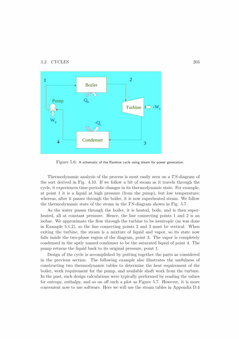
5.2. CYCLES 203
Boiler
Condenser
TurbinePump
1 2
34
Qb
-Ws
-QcWp
Figure 5.6: A schematic of the Rankine cycle using steam for power generation.
Thermodynamic analysis of the process is most easily seen on a TS-diagram ofthe sort derived in Fig. 4.10. If we follow a bit of steam as it travels through thecycle, it experiences time-periodic changes in its thermodynamic state. For example,at point 1 it is a liquid at high pressure (from the pump), but low temperature;whereas, after it passes through the boiler, it is now superheated steam. We followthe thermodynamic state of the steam in the TS-diagram shown in Fig. 5.7.
As the water passes through the boiler, it is heated, boils, and is then super-heated, all at constant pressure. Hence, the line connecting points 1 and 2 is anisobar. We approximate the flow through the turbine to be isentropic (as was donein Example 5.1.2), so the line connecting points 2 and 3 must be vertical. Whenexiting the turbine, the steam is a mixture of liquid and vapor, so its state nowfalls inside the two-phase region of the diagram, point 3. The vapor is completelycondensed in the aptly named condenser to be the saturated liquid of point 4. Thepump returns the liquid back to its original pressure, point 1.
Design of the cycle is accomplished by putting together the parts as consideredin the previous section. The following example also illustrates the usefulness ofconstructing two thermodynamic tables to determine the heat requirement of theboiler, work requirement for the pump, and available shaft work from the turbine.In the past, such design calculations were typically performed by reading the valuesfor entropy, enthalpy, and so on off such a plot as Figure 5.7. However, it is moreconvenient now to use software. Here we will use the steam tables in Appendix D.4
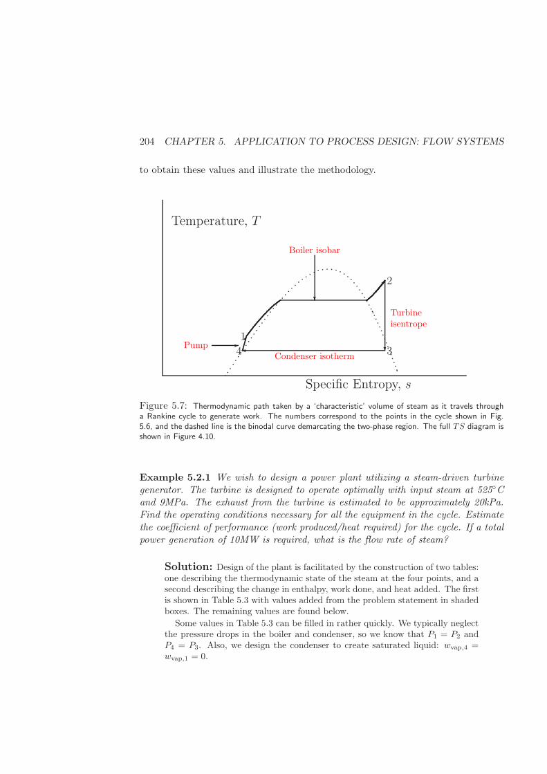
204 CHAPTER 5. APPLICATION TO PROCESS DESIGN: FLOW SYSTEMS
to obtain these values and illustrate the methodology.
Temperature, T
Specific Entropy, s
2
4
1
3
Boiler isobar
Turbineisentrope
Condenser isothermPump ?
7?
-
Figure 5.7: Thermodynamic path taken by a ‘characteristic’ volume of steam as it travels througha Rankine cycle to generate work. The numbers correspond to the points in the cycle shown in Fig.5.6, and the dashed line is the binodal curve demarcating the two-phase region. The full TS diagram isshown in Figure 4.10.
Example 5.2.1 We wish to design a power plant utilizing a steam-driven turbinegenerator. The turbine is designed to operate optimally with input steam at 525Cand 9MPa. The exhaust from the turbine is estimated to be approximately 20kPa.Find the operating conditions necessary for all the equipment in the cycle. Estimatethe coefficient of performance (work produced/heat required) for the cycle. If a totalpower generation of 10MW is required, what is the flow rate of steam?
Solution: Design of the plant is facilitated by the construction of two tables:one describing the thermodynamic state of the steam at the four points, and asecond describing the change in enthalpy, work done, and heat added. The firstis shown in Table 5.3 with values added from the problem statement in shadedboxes. The remaining values are found below.
Some values in Table 5.3 can be filled in rather quickly. We typically neglectthe pressure drops in the boiler and condenser, so we know that P1 = P2 andP4 = P3. Also, we design the condenser to create saturated liquid: wvap,4 =wvap,1 = 0.
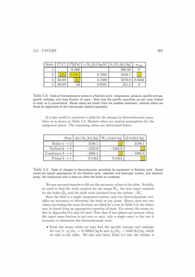
5.2. CYCLES 205
State T [C] P [kPa] s/Mw[kJ/kg·K] h/Mw[kJ/kg] wvap
1 9, 000 260.59 0
2 525 9,000 6.7388 3448.7 1
3 60.09 20 6.7388 2219.8 0.8346
4 60.09 20 0.8321 251.5 0
Table 5.3: Table of thermodynamic states in a Rankine cycle: temperature, pressure, specific entropy,specific enthalpy, and mass fraction of vapor. Note that the specific quantities are per mass insteadof mole, as is conventional. Boxed values are known from the problem statement, whereas others arefound by application of the macroscopic balance equations.
It is also useful to construct a table for the changes in thermodynamic quan-tities as is shown in Table 5.4. Shaded values are typical assumptions for theequipment pieces. The remaining values are determined below.
Step ∆h/Mw[kJ/kg] Ws/m[kJ/kg] Q/m[kJ/kg]
Boiler:1 → 2 3188.1 0 3188.1
Turbine:2 → 3 −1228.9 −1228.9 0
Condenser:3 → 4 −1968.3 0 −1968.3
Pump:4 → 1 9.1344 9.1344 0
Table 5.4: Table of changes in thermodynamic quantities for equipment in Rankine cycle. Boxedvalues are typical assumptions for the Rankine cycle: adiabatic and isentropic turbine, and adiabaticpump. No mechanical work is done on either the boiler or condenser.
We now proceed stepwise to fill out the necessary values in the table. Notably,we need to find the work required for the pump Wp, the heat input required
for the boiler Qb, and the shaft work obtained from the turbine −Ws.Since the fluid is a single component system, only two thermodynamic vari-
ables are necessary to determine the state at any point. Hence, once any twovalues (excluding the mass fraction) are filled for a row in Table 5.3, the othersmay be found from an appropriate equation of state. For steam, the steam ta-bles in Appendix D.4 may be used. Note that if two phases are present (whenthe vapor mass fraction is not zero or one), only a single entry in the row isnecessary to determine the thermodynamic state.
• From the steam tables we may find the specific entropy and enthalpyfor row 2: s2/Mw = 6.7388kJ/kg·K and h2/Mw = 3448.7kJ/kg, whichwe add to the table. We also note from Table 5.4 that the turbine is
206 CHAPTER 5. APPLICATION TO PROCESS DESIGN: FLOW SYSTEMS
assumed isentropic, so that we can immediately adds3/Mw = s2/Mw =6.7388kJ/kg·K to the table.
• Since we know the pressure and entropy of point 3, we may now de-termine, using the steam tables, the remaining quantities in this row.When we check the tables, we find that at P3 = 20kPa, the entropy atpoint 3 falls between the values of entropy for the vapor and the liquid.Hence, the water must be a mixture of liquid and vapor, as is shownin Fig. 5.7. From the steam tables, svap[20kPa]/Mw = 7.9094kJ/kg·K,and sliq[20kPa]/Mw = 0.8321kJ/kg·K. Hence, we can find the vapor massfraction from
s3 = wvapsvap + (1 − wvap)sliq,
to be wvap = 0.8346. Using an analogous equation for enthalpy, we canalso find h3/Mw = 2219.8kJ/kg. Using the tables for saturated steam, weestimate the temperature at this point to be 60.09C.
• We note that the values for enthalpy in Table 5.3 can be used to find thechange in enthalpy 2 → 3 for Table 5.4: ∆h2→3/Mw = h3/Mw−h2/Mw =−1228.9kJ/kg. A macroscopic energy balance on the turbine yields
Ws
m= ∆h2→3/Mw,
which allows us to fill in the shaft work delivered by the turbine.
• We can also find the thermodynamic state at 4, which is the saturatedliquid from point 3. Hence, we immediately write down T4 = 60.09C,P4 = 20kPa, s4/Mw = sliq[20kPa]/Mw = 0.8321kJ/kg·K, and h4/Mw =hliq[20kPa]/Mw = 251.5kJ/kg.
• Again, we use the enthalpies from rows 3 and 4 of the first table to obtainthe change in enthalpy in the second table: ∆h3→4/Mw = h4/Mw −h3/Mw = −1968.3kJ/kg. An energy balance on the condenser yields
Qc
m= ∆h3→4/Mw,
from which we fill in the condenser duty in Table 5.4.
• We find the pump specifications as we did in Example 5.1.3
Wp
m≈ v4(P1 − P4)/Mw.
Hence, we find that Wp/m ≈ 9.1344kJ/kg. An energy balance on thepump yields
Wp/m = ∆h4→1/Mw,
which allows us to fill in the change in enthalpy, and h1/Mw = 260.6kJ/kg.
5.2. CYCLES 207
• Finally, an energy balance yields the heat duty on the boiler
Qb
m= ∆h1→2/Mw = h2/Mw − h1/Mw,
from which we find Qb/m = 3188.1kJ/kg.
With the second table completed, we can now find the coefficient of perfor-mance for the cycle εc, which is the ratio of available work to the heat duty ofthe boiler
εc :=−Ws − Wp
Qb
, (5.55)
which yields 38.3% efficiency for this cycle. We can compare this to the maxi-mum efficiency that would be attained by a Carnot cycle that operates betweenthe temperature output by the boiler and the temperature of the condenser.Using Eqn. (5.53), we find the maximum coefficient of performance for thisexample is
εCarnot = 1− T3T2
= 0.582, (5.56)
or 58.2% efficiency.We find the necessary flow rate of steam from the desired Ws = −10MW=
10, 000kJ/s, and the calculated Ws/m = −1228.9 to be m = 8.14kg/s. 2
A real cycle operates less efficiently than this, however, because of heat lossesin the turbine, entropy generation in the turbine and pump, and the fact that theheat reservoirs must have different temperatures from the condenser and boiler inorder to drive heat flows.
5.2.3 The Refrigeration Cycle
Refrigeration has the opposite goal of a power cycle. Instead of adding heat tothe cycle in order to extract work, we add work in order to extract heat. Herewe consider an evaporation cycle that uses a single component fluid. When wemanipulate the pressure of the fluid, we can cause it to condense to give off heatin one part of the cycle, and to evaporate in another part of the cycle in order toextract heat from, say a refrigerator. Work is required to compress the fluid andcondense. Schematically, the cycle is shown in Figure 5.8. In this cycle a valve (orthrottle) is used to cause the pressure drop and evaporate the fluid. The changes inthe state of the fluid can be illustrated on a PH diagram such as is shown in Figure5.9. The sketch shows that we assume an isentropic compressor, isobaric evaporatorand condenser, and an isenthalpic throttle.
In the following example we use ammonia to refrigerate a freezer to −15C.As is customary in refrigeration, we use a PH diagram to aid in our design. The
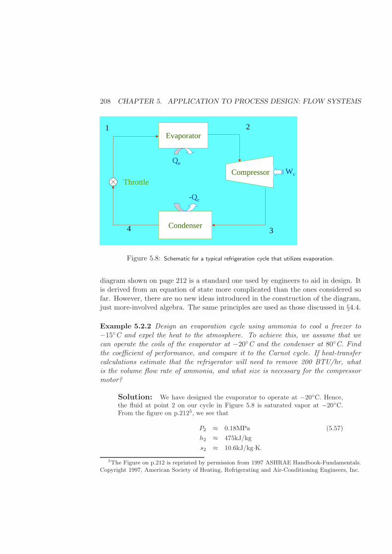
208 CHAPTER 5. APPLICATION TO PROCESS DESIGN: FLOW SYSTEMS
Evaporator
Condenser
Compressor
1 2
34
Qe
Wc
-Qc
Throttle
Figure 5.8: Schematic for a typical refrigeration cycle that utilizes evaporation.
diagram shown on page 212 is a standard one used by engineers to aid in design. Itis derived from an equation of state more complicated than the ones considered sofar. However, there are no new ideas introduced in the construction of the diagram,just more-involved algebra. The same principles are used as those discussed in §4.4.
Example 5.2.2 Design an evaporation cycle using ammonia to cool a freezer to−15C and expel the heat to the atmosphere. To achieve this, we assume that wecan operate the coils of the evaporator at −20C and the condenser at 80C. Findthe coefficient of performance, and compare it to the Carnot cycle. If heat-transfercalculations estimate that the refrigerator will need to remove 200 BTU/hr, whatis the volume flow rate of ammonia, and what size is necessary for the compressormotor?
Solution: We have designed the evaporator to operate at −20C. Hence,the fluid at point 2 on our cycle in Figure 5.8 is saturated vapor at −20C.From the figure on p.2125, we see that
P2 ≈ 0.18MPa (5.57)
h2 ≈ 475kJ/kg
s2 ≈ 10.6kJ/kg·K.5The Figure on p.212 is reprinted by permission from 1997 ASHRAE Handbook-Fundamentals.
Copyright 1997, American Society of Heating, Refrigerating and Air-Conditioning Engineers, Inc.
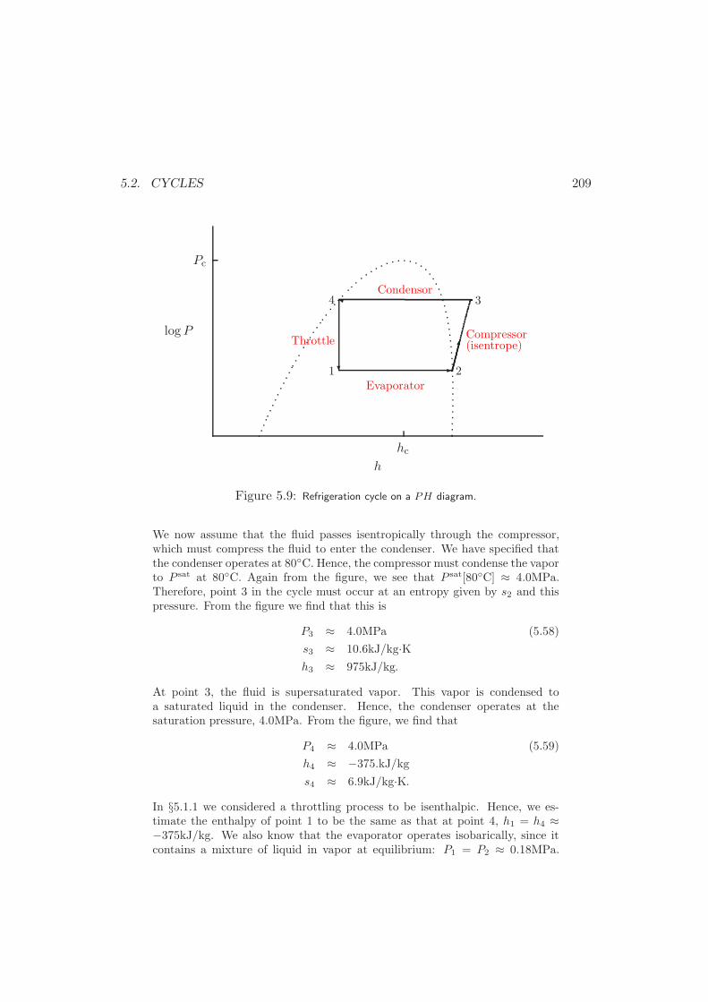
5.2. CYCLES 209
Pc
hc
logP
h
2
34
1
Compressor
Evaporator
Condensor
Throttle (isentrope)
y
? -
Figure 5.9: Refrigeration cycle on a PH diagram.
We now assume that the fluid passes isentropically through the compressor,which must compress the fluid to enter the condenser. We have specified thatthe condenser operates at 80C. Hence, the compressor must condense the vaporto P sat at 80C. Again from the figure, we see that P sat[80C] ≈ 4.0MPa.Therefore, point 3 in the cycle must occur at an entropy given by s2 and thispressure. From the figure we find that this is
P3 ≈ 4.0MPa (5.58)
s3 ≈ 10.6kJ/kg·Kh3 ≈ 975kJ/kg.
At point 3, the fluid is supersaturated vapor. This vapor is condensed toa saturated liquid in the condenser. Hence, the condenser operates at thesaturation pressure, 4.0MPa. From the figure, we find that
P4 ≈ 4.0MPa (5.59)
h4 ≈ −375.kJ/kg
s4 ≈ 6.9kJ/kg·K.
In §5.1.1 we considered a throttling process to be isenthalpic. Hence, we es-timate the enthalpy of point 1 to be the same as that at point 4, h1 = h4 ≈−375kJ/kg. We also know that the evaporator operates isobarically, since itcontains a mixture of liquid in vapor at equilibrium: P1 = P2 ≈ 0.18MPa.
210 CHAPTER 5. APPLICATION TO PROCESS DESIGN: FLOW SYSTEMS
These two values determine the location on the figure, and we can write downall of the thermodynamic quantities. We find that the point lies inside thebinodal region. Hence, the fluid is here a mixture of liquid and vapor.
h1 = h4 ≈ −375.kJ/kg (5.60)
P1 = P2 ≈ 0.18MPa
We can find the mass fraction of vapor xvap from this enthalpy by noting
h1 = wvaphvap1 + (1− wvap)hliq1 . (5.61)
We find from the figure that
hvap1 = h2 ≈ 475kJ/kg, (5.62)
hliq1 ≈ −850.kJ/kg.
Hence, we find wvap ≈ 0.358 from the last three equations.From the thermodynamic states at all of the points, we can now find the
work and heat in the different components. From the energy balance on thecompressor, we find that
Wc
m=
∆h2→3
Mw=h3 − h2Mw
≈ 500kJ/kg. (5.63)
From an energy balance on the evaporator we find
Qem
=∆h1→2
Mw=h2 − h1Mw
≈ 850kJ/kg. (5.64)
Our design requires that the heat transfer rate be 200 BTU/hr. Hence, we findthat the mass flow rate of the fluid should be
m =Qe
Qe/m≈(200BTU/hr
850kJ/kg
)
(1.055kJ/BTU) = 250g/hr. (5.65)
Using our energy balance on the compressor, we find that the pump in thecompressor uses
Wc = m
(
Wc
m
)
≈ (0.25kg/hr)(500kJ/kg) = 125kJ/hr. (5.66)
We can calculate the coefficient of performance for refrigeration, which is theratio of heat removed to work required
εr =Qe
Wc
≈ 1.7, (5.67)

5.3. SUMMARY 211
which can be compared to the Carnot performance, Eqn. (5.54)
εCarnot =Tc
Th − Tc= 2.53, (5.68)
where we have taken the cold and hot reservoirs to be −20C and 80C, re-spectively, instead of the temperature of the freezer and ambient. 2
For very large systems, it can be more economical to replace the throttle with aturbine to get some work back out of the fluid at this step. The extracted work canthen be used to help run the compressor and lower operating costs. This changesthe thermodynamic analysis in step 4 → 1. Instead of being isenthalpic, the step isisentropic.
5.3 Summary
In this chapter we applied the ideas of thermodynamics to flowing systems whenone can safely assume local equilibrium. Applying this assumption to tiny volumeelements, we derived the microscopic balance equations for density, energy, velocityand entropy in Appendix C. By integrating these equations over a larger controlvolume we derived the macroscopic balance equations in §5.1. These macroscopicbalance equations are then used to find approximate solutions to large flowing sys-tems. After completion of this chapter, the student should be able to analyze thethermodynamic limitations of any flowing system that is well approximated as beingin local equilibrium.
Most of the chapter is devoted to solving specific problems. Those consideredare
• The flow of butane through a valve (the throttling process).
• Work in a steam-driven turbine.
• The work requirements for a pump.
• The thermodynamic analysis of an ideal gas in a Ranque-Hilsch vortex tube.
• The available electrical work in a fuel cell.
• The thermodynamic analysis of a Carnot cycle, the Rankine power cycle usingsteam, and a refrigeration cycle using ammonia.
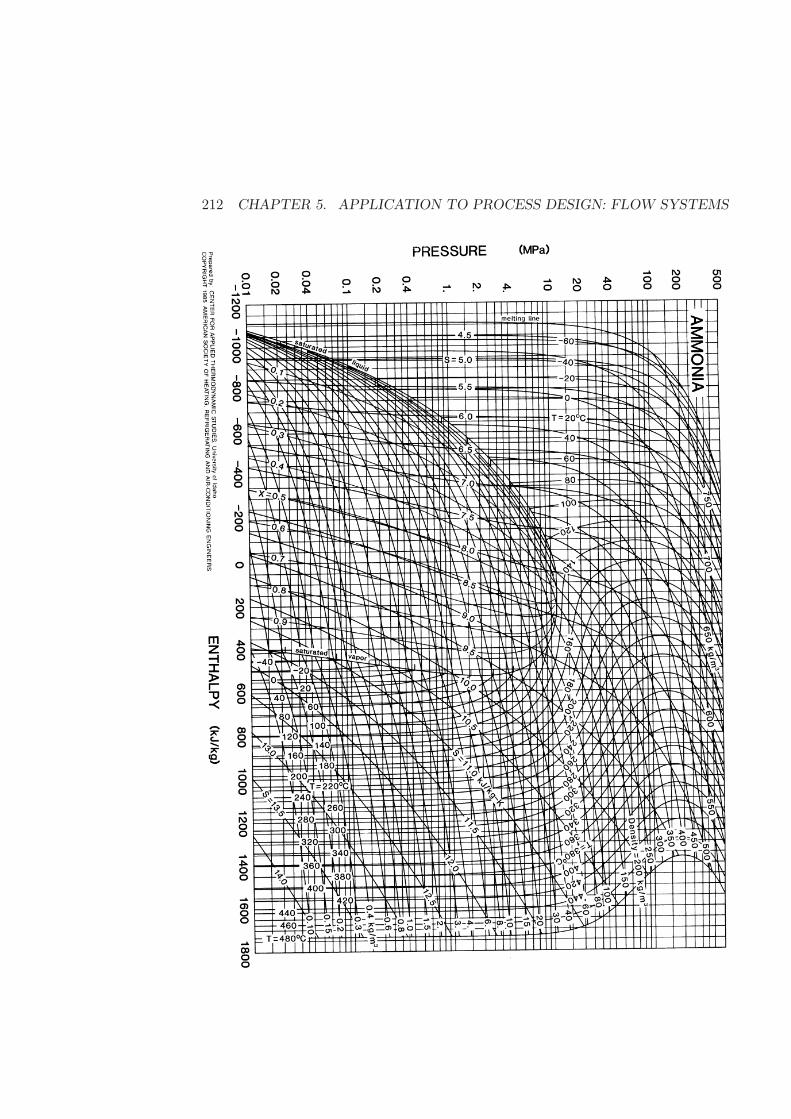
212 CHAPTER 5. APPLICATION TO PROCESS DESIGN: FLOW SYSTEMS
5.4. EXERCISES 213
5.4 Exercises
5.1.A. You want to power a 60W light bulb with a methanol fuel cell stack of225 cm2 connected in series. Use the data provided in Table 5.1, and possibly theresults from Example 5.1.5, to design a fuel cell stack to power it. Do you want yourfuel cells to be stacked in series (keeping current constant, but changing voltage),or in parallel (keeping voltage constant, but changing current). Aside from givingthe necessary quantitative answers (e.g., number of cells, operating voltage, etc.),explain in detail how you chose the optimal operating conditions for the cells. Forexample, at what efficiency would your stack operate?
5.1.B. Consider the turbine in Example 5.1.2.
(1) Suppose that the entropy generation is neglected, but that the heat loss fromthe turbine −Q is assumed to be 10% of the generated work. Further assume thatthe heat loss occurs completely at the inlet temperature. Calculate the mass flowrate and exit conditions of the steam. Is the turbine more or less efficient than theadiabatic case?
(2) What are the exit conditions and flow rates if you assume that the entropygeneration is equivalent to the entropy loss along the sides of the turbine?
(3) Finally, assume that the turbine operates adiabatically, but that the entropygeneration inside the turbine is approximately 0.10Ws/Ti. Now find the exit condi-tions of the steam and the required mass flow rates. How good is the ideal estimate,and how important is it to estimate accurately the entropy generation?
5.1.D. Steam at temperature Ti = 400C and pressure Pi = 9.8MPa is fed to avortex tube. If the hot and cold streams have the same mass flow rates and pressurePf = 2.0MPa, what range of temperatures is thermodynamically permissible for theexit streams?
5.1.E. Nitrogen at temperature Ti = 400C and pressure Pi = 9.8MPa is fed to avortex tube. If the hot and cold streams have the same mass flow rates and pressurePf = 2.0MPa, what range of temperatures is thermodynamically permissible for theexit streams? Use the Peng-Robinson equation of state for your estimate.
5.1.F. R. Hilsch suggested that the efficiency of the Ranque-Hilsch vortex tube bemeasured by taking the ratio of the temperature drop in the cold stream T0−Tc, overthe temperature drop that would occur for an isentropic expansion of the gas from(T0, P0) to Tatm. What is the efficiency of the Ranque-Hilsch vortex tube consideredin Example 5.1.4?
5.1.G. Your bicycle tire is pumped to 65psi and the temperature is 25C. Whenyou open the valve, what is the temperature of the air coming out, if you assume itis all nitrogen?

214 CHAPTER 5. APPLICATION TO PROCESS DESIGN: FLOW SYSTEMS
Inlet P Valve Pos. Th Tc Ti Vol. flow in Vol. flow cold(psig) (degrees) (C) (C) (C) (l/min) (l/min)
16.8 0 31.8 28.8 30.2 14.05 12.516.8 30 34.2 23.0 30.2 15.1 11.116.8 60 36.2 22.8 30.2 15.3 8.445. 0 43.6 16.6 30.6 33.2 30.45. 30 46.6 7.6 30.8 33.4 24.945. 60 49.4 12.2 30.8 33.8 20.65. 0 39.4 3.8 30.2 48.8 41.465. 30 45.2 -3.6 30.6 49.6 33.565 60 50.4 4.2 30.2 50.1 26.1
Table 5.5: Measured quantities for a vortex tube with adjustable position of inlet valve. The entries,from left to right, are inlet pressure, position of inlet valve, temperature of exiting hot stream, pressureof exiting cold stream, temperature of inlet stream, volumetric flow rate in, and volumetric flow rateout.
5.1.H. In Example 5.1.1, we held the lighter so that liquid butane entered the valve.If we hold the lighter so that vapor enters the valve, what would the temperatureof the exiting stream be? Use the Peng-Robinson equation of state for the vaporinside the lighter.
5.1.I. A vortex tube using compressed air is operated, and data on the inlet andoutlet streams are gathered. Table 5.5 shows the properties of these streams. Wewish to analyze the performance of the tube assuming that air is an ideal gas atthese conditions, and that its properties may be estimated as a mixture of 80%nitrogen and 20% oxygen. To perform the analysis, first find the mass flow rates ofthe streams given, and then estimate the mass flow rate of the remaining stream.Then perform an energy balance on the system. Is it operated adiabatically? Nextperform an entropy balance and determine if entropy generation is zero, positive,or negative. Make plots of Q/m versus valve position, and entropy generation permass versus valve position, each for several inlet pressures. Is there any correlationbetween entropy generation and the temperature of the cold stream? What roledoes heat flow play?
5.2.A. Using a steam-driven Rankine cycle, design a power plant to deliver 1.5 MWof power. Assume that the turbine operates with input steam at 475C and 5MPa,and that the exit stream is at 25kPa. What is the coefficient of performance?
5.2.B. Design a steam power plant using the Rankine cycle. Assume that the tur-bine operates with entering and exiting pressures of 7.25MPa and 5kPa, respectively.The entering temperature of the steam is 425C. Find the operating conditions of
5.4. EXERCISES 215
all the components in the cycle. Find the coefficient of performance, and compareit to the Carnot efficiency. If a total power generation of 625kW is required fromthe cycle, what is the mass flow rate of steam necessary?
5.2.C. Find the coefficient of performance, evaporator duty, and compressor size ifthe throttle in Example 5.2.2 is replaced by a turbine. Assume that the turbine isused to help power the compressor.
5.2.D. Design a steam power plant using the Rankine cycle assuming that theturbine operates with an entering pressure of 6.1MPa, an entering temperature of510C, and an exiting pressure of 1.5kPa. Find the operating conditions of the fluideverywhere in the cycle, the coefficient of performance, and compare it to a Carnotcycle operating at the same temperatures. If 310kW of power is required, what flowrate of steam is necessary?
5.2.E. We wish to use a refrigerant from DuPont (HCFC-123) to design a refriger-ation cycle. Thermodynamic properties of the fluid can be found at
http://www.dupont.com/suva/na/usa/literature/pdf/h47753.pdf.Design a refrigeration cycle to operate between 40 and 140F. While the pump is
running, the refrigerator should provide 1000BTU/hr cooling capacity. What flowrate of refrigerant is necessary, and what size pump is needed?
5.2.F. Analyze the Carnot cycle in reverse (i.e., as a refrigerator) to obtain thecoefficient of performance expression given in Eqn. (5.54).

216 CHAPTER 5. APPLICATION TO PROCESS DESIGN: FLOW SYSTEMS
Chapter 6
Statistical Mechanics
In this chapter, we make the connection between molecules and thermodynamics.Until this chapter, we have dealt only with macroscopic quantities, and the in-fluence of molecular details has been discussed only qualitatively. Here, we makequantitative connections between molecules, and much of the thermodynamics wehave already seen. For example, we derive the fundamental relations for ideal gases(simple and general), molecular adsorption on solid surfaces, and the elasticity ofpolymer chains. The procedure is general, and may be used to derive fundamentalrelations for more complex systems, to relate macroscopic experimental results tomolecular interactions, or to exploit computer simulations. Since statistical me-chanics deals with more detailed information than does classical thermodynamics,we can also find how real systems fluctuate in time when at equilibrium. We willsee that these fluctuations are important for all systems, and can even dominate thebehavior of fluids near a critical point (or spinodal curve) or that of small systems.
This chapter is not essential for understanding most of the rest of the book.However, the remaining chapters will also have a few sections dealing with thestatistical mechanics of mixtures and polymers, and the material in this chapteris essential for understanding those topics. Statistical mechanics is both beautifuland powerful, but often difficult to grasp the first time you see it. However, webelieve that statistical mechanics, like thermodynamics, rewards the student whovisits it repeatedly. Therefore, we include a short introduction to the subject here,and encourage the student to try and capture a rough idea of how it works. If thedetails are baffling at first, try instead to capture what goes in to the modelling,what assumptions are made, and what comes out at the end.
217
218 CHAPTER 6. STATISTICAL MECHANICS
6.1 Ensemble and Time Averages
Most of the systems of interest in this text consist of collections of a large numberof molecules (of order 1023). These molecules are moving incessantly, and yet themacroscopic equilibrium thermodynamic properties are stable in that they neitherchange with time nor become heterogeneous. The reason for this is that, in simplefluids, molecular motion occurs on time scales that are much faster than thoseassociated with macroscopic measurements; that is, our macroscopic probes areinsensitive to fast processes and only measure “average” properties of a collection ofmolecules. This observation suggests that the behavior of a collection of moleculescould be analyzed using statistical methods, thereby allowing us to extract averagequantities and the magnitude of fluctuations around the mean.
Figure 6.1 shows the instantaneous internal energy of a collection of just 200“Lennard-Jones” molecules (a good model for the behavior of simple fluids such asargon or methane) as a function of reduced time. The energy undergoes rapid fluc-tuations about a mean value. The time scale for these fluctuations is relatively fast(on the order of 10−15 s); the whole abscissa comprises events that happened withinjust a fraction of a nanosecond. As the number of molecules increases, the size of thefluctuations decreases relative to the mean energy, roughly as the square root of theinverse of the number of molecules. A macroscopic measurement technique for theenergy would be unable to resolve these fast fluctuations and it would only samplean average internal energy value. The methods of statistical mechanics allow us todo precisely that. The statistical properties of collections or ensembles of moleculesare studied in order to make predictions about the average value of thermodynamicproperties and the likelihood of observing deviations from that average.
Following our development of classical thermodynamics presented in previouschapters, we begin by introducing a postulate. That postulate states that, for anisolated system, all microscopic states having the same volume, number of molecules,and energy are equally likely to occur.
Statistical Postulate I: For an isolated system consisting of N molecules,having volume V and energy U , all microscopic states consistent with thoseconstraints occur with the same probability.
Let’s consider an example. Think of a collection of N molecules of a noble gas(e.g., Argon) confined to a small container with volume V . Furthermore, we canassume that the container is well insulated, so as to prevent interactions with theexterior, thereby maintaining a constant energy. At any non-zero temperature, themolecules in the container are constantly moving and exchanging energy with oneanother, but the total energy must somehow remain constant. This is equivalent to
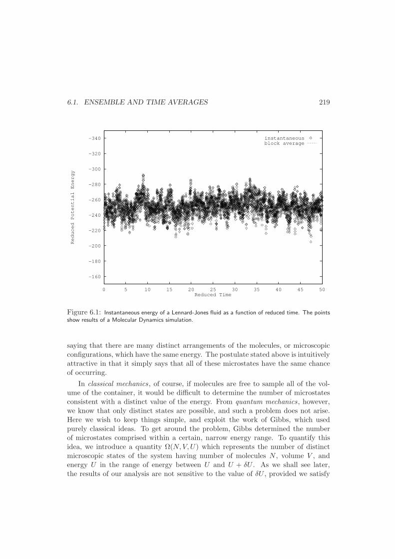
6.1. ENSEMBLE AND TIME AVERAGES 219
-340
-320
-300
-280
-260
-240
-220
-200
-180
-160
0 5 10 15 20 25 30 35 40 45 50
Reduced Potential Energy
Reduced Time
instantaneousblock average
Figure 6.1: Instantaneous energy of a Lennard-Jones fluid as a function of reduced time. The pointsshow results of a Molecular Dynamics simulation.
saying that there are many distinct arrangements of the molecules, or microscopicconfigurations, which have the same energy. The postulate stated above is intuitivelyattractive in that it simply says that all of these microstates have the same chanceof occurring.
In classical mechanics, of course, if molecules are free to sample all of the vol-ume of the container, it would be difficult to determine the number of microstatesconsistent with a distinct value of the energy. From quantum mechanics, however,we know that only distinct states are possible, and such a problem does not arise.Here we wish to keep things simple, and exploit the work of Gibbs, which usedpurely classical ideas. To get around the problem, Gibbs determined the numberof microstates comprised within a certain, narrow energy range. To quantify thisidea, we introduce a quantity Ω(N,V,U) which represents the number of distinctmicroscopic states of the system having number of molecules N , volume V , andenergy U in the range of energy between U and U + δU . As we shall see later,the results of our analysis are not sensitive to the value of δU , provided we satisfy
220 CHAPTER 6. STATISTICAL MECHANICS
the constraints 0 < δU ≪ U . If we use pj to denote the probability of observing adistinct micro-state j of a system having N , V , and energy between U and U + δUat equilibrium, we can write
pj =1
Ω(N,V,U), (6.1)
since the probability must be normalized to sum up to unity. A system for whichN , V , and U are constant is called a microcanonical ensemble . The quantityΩ(N,V,U) is called the microcanonical partition function.
To make a connection with thermodynamics, we introduce the second and finalpostulate of statistical mechanics. It seems intuitively plausible that the entropyof a system would depend on the number of available microstates—a measure ofdisorder. On the other hand, if we double the size of a system, the number ofmicrostates grows quadratically. Since entropy must grow only linearly with size (itis extensive), Boltzmann introduced the postulate
Statistical Postulate II:
S = kB log Ω(U, V,N). (6.2)
The constant kB appearing in Eqn. (6.2) is called Boltzmann’s constant. Ananalysis of experimental data reveals that its value is approximately 1.381 × 10⁻¹⁶
erg/K, which, not coincidentally, is the ideal gas constant divided by Avogadro’snumber. The presence of kB merely gives entropy the correct units, that is theunits that are used in classical thermodynamics. We will see later why this isa sensible definition, and we will show that it is consistent with nature, and ourearlier postulates. As articulated by Richard Feynman in his Lectures on Physics[30], “...entropy is just the logarithm of the number of ways of internally arranging asystem while having it look the same from the outside.” Isn’t that great? To performstatistical mechanics you only have to be able to count! Unfortunately, we shall seethat counting is not as easy as it sounds, because the numbers are so large. Forexample, if the entropy is on the order of the ideal gas constant, then log Ω ∼ NA,Avogadro’s number. Hence, the number of microstates is approximately exp
(1023
).
6.2 The Canonical Ensemble
The purpose of the statistical mechanical formalism presented in this text is ulti-mately that of providing a useful framework in which to analyze the structure andproperties of molecular-level systems. This framework would of course be used to
6.2. THE CANONICAL ENSEMBLE 221
interpret experimental data, and in that respect the microcanonical ensemble is notthe most convenient to work with.
As we considered in earlier chapters, experiments are often conducted at constanttemperature, volume, and number of molecules. An ensemble in which these threevariables are kept constant is called a canonical ensemble. To derive a partitionfunction for this ensemble, we can go through the following thought experiment.Consider a subsystem, or group of molecules, immersed in a giant thermal reservoirwhose energy is Ubath. The energy of the subsystem fluctuates through interactionswith the thermal bath, but the energy of the total system remains constant. If, forsimplicity, we assume that the energy of the subsystem adopts discrete values1 Uj ,then we have
Utotal = Ubath + Uj , constant, (6.3)
where the total energy is constant because the combined system is isolated. Wenow wish to determine the probability that the subsystem has energy Uj . Theentire system is isolated, so the probability pj,k that the subsystem is in state j, andthe reservoir is in state k is found from the postulate
pj,k =1
Ωtotal[Utotal]. (6.4)
To find the probability pj that the subsystem is in state j, and the reservoir is inany other state, we sum this probability over all reservoir states
pj =∑
k
pj,k
=∑
k
1
Ωtotal[Utotal]
=Ωbath[Utotal − Uj ]
Ωtotal[Utotal]. (6.5)
We used the property of probabilities to write the first line, and Eqn. (6.4) to obtainthe second. To obtain the last line we used the fact that Ωtotal is independent ofthe particular energy distribution between subsystem and reservoir, and the defi-nition of Ωbath. Namely, Ω[Utotal] is the total number of distinct configurations ofthe combined system, and where Ωbath[Utotal − Uj] is the number of configurationsavailable to the reservoir when the subsystem has energy Uj. We have suppressedarguments involving the volume and mole numbers in the bath and subsystem, be-cause these are held constant. The quantity pj is nothing other than the fraction of
1Actually, from quantum mechanics we know that real systems can adopt only discrete valuesfor energy.
222 CHAPTER 6. STATISTICAL MECHANICS
the total number of configurations of the total system in which the subsystem is ina configuration having energy Uj .
The probability pj can be related to the entropy of the bath and that of the totalsystem through Eqn.(6.2). Upon substitution of that expression into Eqn.(6.5) wehave
pj = exp
[Sbath[Utotal − Uj ]− Stotal[Utotal]
kB
]
. (6.6)
The total entropy of the system consists of the entropy of the subsystem and that ofthe reservoir. At equilibrium, the energy of the subsystem immersed in the reservoirundergoes rapid fluctuations around some average value, Uavg. In order to determinethe entropy of the subsystem we resort to thermodynamics and calculate the entropycorresponding to that average value of the energy. Following that reasoning we write
Stotal[Utotal] = S[Uj] + Sbath[Utotal − Uj], (6.7)
since entropy is extensive. According to the definition of a heat reservoir, the fluctu-ations in energy exchanged with the subsystem are infinitesimally small. FollowingCallen [13, p.350], the energy of the reservoir can then be expanded about its averagevalue to give
Sbath[Utotal − Uj] ∼= Sbath[Utotal − Uavg] + (Uavg − Uj)
(∂Sbath∂U
)
Vbath,Nbath
∣∣∣∣∣U=Utot−Uavg
= Sbath[Utotal − Uavg] +Uavg − Uj
T. (6.8)
Upon substitution of Eqn.(6.8) into Eqn.(6.6) the probability pj becomes
pj = exp
[Sbath[Utotal − Uavg]− Stotal[Utotal]
kB
]
exp
[Uavg − UjkBT
]
. (6.9)
We can now use the fact that entropy is extensive to eliminate the entropies of thecombined system and the bath above to obtain
pj = exp
[Uavg − TS[Uavg]
kBT
]
exp
[
− UjkBT
]
. (6.10)
The quantity Uavg − TS[Uavg] corresponds to the Helmholtz free energy of the sub-system, F . Note what we have accomplished: the bath influences this last expressiononly through the temperature T .
We can now find an expression for the free energy; the sum over all possibleconfigurations of the probability pj must be unity
∑
j
pj = exp
(F
kBT
)∑
j
exp
(
− UjkBT
)
= 1. (6.11)
6.2. THE CANONICAL ENSEMBLE 223
The free energy of the system is therefore given by
F
kBT= − logQ(T, V,N), (6.12)
where the quantity Q is called the canonical-ensemble partition function, andis given by
Q(T, V,N) :=∑
j
exp (−Uj/kBT ) . (6.13)
JDS: This notationconflicts with heattransfer. Perhaps amore robust notationwould be somethinglike ∆F , ∆G, ∆ψ,etc.
The partition function plays a central role in statistical mechanics. It should not beconfused with heat; which quantity is meant by Q should be clear from the context.We hate it when books confuse notation, but this choice of notation for the partitionfunction is so ubiquitous in the nature (or even worse, the notation Z is used), thatwe are willing to make an exception here. Also, problems practically never arisewhere both the partition function and heat flow appear at the same time.
We see from Eqn. (6.12) that knowledge of Q(T, V,N) yields a fundamentalrelation. Eqn. (6.13) shows us how to find it. Similarly, we can see that Ω(U, V,N)also yields a fundamental relation from Statistical Postulate II. Hence, it is calledthe microcanonical partition function. The bulk of statistical mechanics is anattempt to estimate partition functions for real systems.
From Eqn. (6.11) we also see that the probability for the system to be in micro-state j is
pj =1
Qexp
(
− UjkBT
)
. (6.14)
It is interesting to find the entropy in terms of the probabilities. Recall from thedifferential for F that
S = −(∂F
∂T
)
V,N
=
(∂
∂TkBT logQ
)
V,N
= kB logQ+kBT
Q
∑
j
UjkBT 2
exp (−Uj/kBT ) , (6.15)
where we used Eqn. (6.12) to obtain the second line, and the definition of thecanonical partition function, Eqn (6.13), to obtain the third. Now we use our result

224 CHAPTER 6. STATISTICAL MECHANICS
for the probability Eqn. refeq:canonical probability) to simplify the second term onthe right side
S = kB logQ+∑
j
UjTpj,
= kB∑
j
pj
[
logQ+UjkBT
]
,
= −kB∑
j
pj log pj . (6.16)
To obtain the second line, we used the fact that the probability is normalized:∑
j pj = 1. The third line used again our expression for pj.
What is interesting about this result is that it also works for the microcanonicalensemble. In other words, if we insert Eqn. (6.1) into Eqn. (6.16), we obtain thesecond statistical mechanical postulate, Eqn. (6.2). In fact, the result above playsan important role not just in thermodynamics, but also in non-equilibrium ther-modynamics [64], information theory [51], applied mathematics [72], and processcontrol.
6.3 Ideal Gases
6.3.1 Simple Ideal Gas
To illustrate the use of statistical mechanics and the canonical ensemble, in thissection we derive the partition function, fundamental relation, and equations ofstate for a simple, monotonic ideal gas. It is easiest to solve this problem using thecanonical ensemble, so we consider a large thermal bath in which a subsystem isimmersed. The number of molecules N and volume V of the subsystem is constant,and the thermal bath holds the temperature fixed. Whereas T , V , and N areconstant, the instantaneous energy of the subsystem fluctuates through interactionswith the thermal bath. The total, instantaneous energy of the subsystem consistsof a sum of kinetic and potential energy terms
U(~rN , ~pN ) = Ukin(~pN ) + Upot(~r
N ). (6.17)
The specific value of the energy corresponding to a particular “configuration” of thesubsystem depends on the positions of the atoms and their momenta, where ~rN :=~r1, ~r2, . . . , ~rN and ~pN := ~p1, ~p2, . . . , ~pN are used to denote collectively the position
coordinates and the momenta of all the N molecules in the system, respectively.
6.3. IDEAL GASES 225
Following the discussion of the previous section, we know that the energy of thesubsystem should be distributed according to the following probability distribution
p(~rN , ~pN ) =1
Qexp
[
−U(~rN , ~pN )
kBT
]
. (6.18)
As we saw in the previous section, the partition function Q is obtained by summingthe exponential terms corresponding to all of the distinct configurations that thesubsystem can adopt. For a large number of molecules in a continuum, the energiesof different configurations are going to be closely spaced, and it is therefore appro-priate to replace the summation appearing in Eqn.(6.13) by an integral over all ofthe coordinates of all the molecules in the subsystem
Q =1
(2πh)3N
∫ ∫
Vexp
(
−U [~rN , ~pN ]
kBT
)
d~rNd~pN . (6.19)
A factor of 1/h3N , where h ∼= 1.0545716× 10⁻³⁴ J·s is the reduced Planck constant,has been included in Eqn.(6.19) to reconcile the classical arguments presented herewith quantum mechanics; as can be seen from Eqn. (6.12), its only impact is toshift the reference state for the free energy by a constant amount proportional to−3N log h. Intuitively, one could think of the presence of Planck’s constant as away of introducing Heisenberg’s uncertainty principle: we cannot subdivide drdpany finer than 2πh in the integral.
We have also introduced the number of molecules N := NNA, where N is theusual mole number, and NA is Avogadro’s number. We have used the shorthand,that
∫. . . d~pN represents 3N integrals—each molecule has three components of mo-
mentum. Although that represents a lot of integrals, we will soon see that it is reallyjust the same integral done many times.
By definition, the molecules of an ideal gas are point particles that do not interactwith each other. The internal energy of an ideal gas is therefore purely kinetic, andthe integral over the position coordinates of the molecules appearing in Eqn.(6.19)
226 CHAPTER 6. STATISTICAL MECHANICS
can be simplified considerably to give a volume factor V for each molecule
Q ∼ 1
(2πh)3N
∫ −∞
−∞
∫
Vexp
(
−U [~rN , ~pN ]
kBT
)
d~rNd~pN
∼ 1
(2πh)3N
∫
Vexp
(
−Upot[~rN ]
kBT
)
d~rN∫ −∞
−∞exp
(
−Ukin[~pN ]
kBT
)
d~pN
∼ 1
(2πh)3N
∫
Vd~rN
∫ ∞
∞exp
(
−Ukin[~pN ]
kBT
)
d~pN , dilute, monotonic gases
∼ V N
(2πh)3N
∫ +∞
−∞exp
(
−Ukin[~pN ]
kBT
)
d~pN
∼ V N
(2πh)3N
[∫ +∞
−∞exp
(
−Umolkin [~p]
kBT
)
d~p
]N
. (6.20)
An important assumption has been made to pass from the second to the third lineabove. Namely, we assume that the particles do not interact with one another, sothat Upot = 0. In real gases this is attained by making the density low. Also, wehave neglected any potential interactions between atoms on a molecule. Therefore,the derivation is restricted to monotonic, low density gases. To see how we wentfrom the third to the fourth line it is instructive to consider the special case whereour volume is a rectangular box with side of lengths Lx, Ly, and Lz
∫
d~rN =
∫
. . .
∫
d~r1 . . . d~rN
=
∫
d~r1 . . .
∫
d~rN
=
(∫
d~r
)N
=
(∫ Lz
0
∫ Ly
0
∫ Lx
0dxdydz
)N
= (LxLyLz)N
= V N (6.21)
The momenta of all the molecules in the gas are independent of each other: Ukin[~pN ] =
∑Ni=1 U
molkin [~pi]; it therefore suffices to perform the integration over the momentum
6.3. IDEAL GASES 227
of one molecule and then factorize the result. The integral for one molecule is then
∫ +∞
−∞exp
(
−Umolkin [~p]
kBT
)
d~p =
∫ ∞
−∞
∫ ∞
−∞
∫ ∞
−∞exp
[
−px2 + py
2 + pz2
2mkBT
]
dpxdpydpz
= [2πmkBT ]32 . (6.22)
With these results, the canonical-ensemble partition function becomes
Q ∼[
V
(2πmkBT
h2
) 32
]N
. (6.23)
The group of variables appearing in Equation (6.23) is generally referred to as thede Broglie thermal wavelength, Λ, defined by
Λ :=
√2πh
(mkBT )1/2. (6.24)
Our discussion so far has assumed that all molecules are distinguishable. Molecules,however, are indistinguishable from each other (they don’t have tags or labels toidentify them). Our expression for the partition function therefore overestimatesthe number of arrangements of the molecules; this can be corrected by dividing theright side of Eqn.(6.23) by N !, which is the number of permutations that we canhave amongst the N molecules (see §A.8.1). With this correction, the free energyof the ideal gas becomes
F
kBT= − logQ
= − log
1
N !
[V
Λ3
]N
≈ −N log
[V
NΛ3
]
− N, (6.25)
where the natural logarithm of N ! was approximated using the fact that logN ! ≈N logN −N for large N (this is the Stirling approximation [1, p.257]).
Eqn. (6.25) is a fundamental relation, so we can use it to find equations of state.For example, the entropy is
S = −(∂F
∂T
)
V,N
= NkB + NkB log
[V
NΛ3
]
+3
2NkB, (6.26)
228 CHAPTER 6. STATISTICAL MECHANICS
and the thermal equation of state is given by
U = F + TS =3
2NRT, (6.27)
where we used the relation R = kBNA. The mechanical equation of state is alsoobtained from
P = −(∂F
∂V
)
N,T
=NkBT
V=NRT
V. (6.28)
These are the equations of state introduced in Chapter 2 for a simple ideal gas, sinceNkB = NR.
Also note how the contribution to the partition function from each molecule isindependent of the others, Eqn. (6.20). This factorization of the partition functioninto contributions from energetically independent parts of the system—in this casenon-interacting molecules—is a general principle. In fact, the principle is used re-peatedly in statistical mechanics, and we use it again in the next example for ageneral ideal gas.
6.3.2 General Ideal Gas
We now show that a general ideal gas is made of molecules that do not interact withone another, but may have atoms within the molecule that do interact. In otherwords, the molecules may have bond vibrational energies, rotational energies, etc.,and are no longer just point particles. Therefore, we can write the energy of justone molecule of type 1 as
E1mol(
~R) +~p · ~p2m1
, (6.29)
where ~R is some vector of dimension 2d describing the internal conformations andmomenta of the polyatomic molecule, and tells us about bond lengths, rotationangles, etc. For example, maybe R1 is the length of a covalent bond, R2 is the anglebetween successive bonds, and R3 is a trans-gauche rotation angle. The momentumof the center of mass of the molecule is denoted by ~p, and the mass of the moleculeof type 1 is m1.
We place one such molecule in a box of volume V . The partition function Q1
for our single polyatomic molecule in a box is then, from the definition of Q
Q1 =1
h3+d
∫ ∫ ∫
exp
[
−E1mol(
~R)
kBT− ~p · ~p
2m1kBT
]
d~rd~pd ~R. (6.30)
6.3. IDEAL GASES 229
The two innermost integrals have already been found for the simple ideal gas, where~r is the position of the center of mass of the molecule. The number of internaldegrees of freedom of the molecule is written as d here. The outermost integral isthe contribution from internal degrees of freedom of the molecule. Hence, we canwrite
Q1 =1
h3+d
∫
d~r ×∫
exp
[
− ~p · ~p2m1kBT
]
d~p×∫
exp
[
−E1mol(
~R)
kBT
]
d ~R
=V (2πm1kBT )
3/2
h3Qint
1 (T ) (6.31)
where
Qint1 (T ) :=
1
hd
∫
exp
[
−E1mol(
~R)
kBT
]
d ~R (6.32)
is the contribution to the partition function from the internal degrees of freedom fora molecule of type 1. Note that it depends only on temperature, and not volume.
Now we add a second molecule of type 1 to our box. The system is dilute so themolecules can be assumed not to interact, and the total energy of the system is now
E1mol(
~R1) +~p1 · ~p12m1
+ E1mol(
~R2) +~p2 · ~p22m1
. (6.33)
We go through the same steps as before, and exploit the fact that the nested integralsjust become products again to find the two-molecules-in-a-box partition function
Q2 =V 2(2πm1kBT )
3
2!h6Qint
1 (T )Qint1 (T ). (6.34)
Since the two molecules are indistinguishable, we divided by a factor of 2! to avoidover-counting. It is now straightforward to generalize this result by adding more andmore molecules to the box, as long as they do not interact significantly. If we addN molecules to the box, all of the same type, then the partition function becomes
Q =V N (2πm1kBT )
3N/2
N !h3N
[Qint
1 (T )]N
. (6.35)
Compare this result to that for the non-interacting, monotonic molecules, Eqn. (6.23).The only change is the addition of the internal contribution to the partition function,Qint
1 which depends only upon temperature.
230 CHAPTER 6. STATISTICAL MECHANICS
Therefore, the fundamental relation for a box of N identical, non-interactingparticles is
F
kBT= − logQ (6.36)
≈ −N log
[
V
N
(2πm1kBT
h2
) 32
]
− N − N logQint1 (T ). (6.37)
We can obtain the mechanical equation of state by taking the derivative of each sideof this equation with respect to V . Since Qint
1 (T ) is independent of V , we againobtain the ideal gas law
P
kBT= −
(∂
∂V
F
kBT
)
T,N
=N
V. (6.38)
However, the thermal equation of state is different,
U
NRT= −T
(∂
∂T
F
NRT
)
V,N
=3
2+d logQint
1 (T )
dT. (6.39)
As a result, we see that a simple ideal gas is a dilute gas of monotonic molecules thatrarely see each other, and a general ideal gas includes dilute polyatomic molecules.The more degrees of freedom within the molecule, the greater Qint
1 (T ) is. In fact,infrared spectroscopy can be used to measure the energetics available to the molecu-lar vibrations, and these energetics can in turn be used to predict the heat capacityto great accuracy [69].
Finally, we mention a general result found by the same procedure. If we have rkinds of non-interacting molecules in our system, we can generally write the partitionfunction as a product of each molecule
Q =
r∏
i=1
Qmoli (T, V )Ni
Ni!, (6.40)
where r is the number of types of molecules, Ni is the number of indistinguishablemolecules of type i, and Qmol
i (T, V ) is the partition function for a molecule of typei, such as that given in Eqs. (6.31) and (6.32).
6.4. LANGMUIR ADSORPTION 231
6.4 Langmuir Adsorption
We consider here the statistical mechanical derivation of the fundamental relationused in §3.7.3 for the adsorption of molecules on a solid surface. Recall that, inLangmuir adsorption, we assume that there are Ms distinct adsorption sites, withN ≤ Ms non-interacting, identical molecules adsorbed.
Since the molecules are non-interacting, the energy of our system Etot can bewritten as
Etot(~rN , ~pN ) =
N∑
i=1
Emol(~ri, ~pi), (6.41)
where Emol is the energy of interaction between the adsorption site and the molecule.The position of molecule i, relative to its site, is given by ~ri, and ~pi is the molecule’smomentum. If the molecule has internal degrees of freedom, they could also beadded to Emol, but we ignore it for the time being. Note, however, that there is nointeraction between molecules adsorbed near each other.
Recall that the partition function is a sum over the possible microstates of thesystem, Eqn. (6.13). For our example here, this sum is a sum not just over theenergies that a molecule can have on a site, but also the sum
∑
dist over the waythat these molecules can be distributed among the sites. As before, we replacethe sums over energies of the sites by integrals. Therefore, we write the partitionfunction as
Q(T, Ms, N ) =∑
dist
∫
. . .
∫
exp
[
−Etot(~rN , ~pN )
kBT
]
d~rNd~pN
h3N(6.42)
The sum is over the ways of distributing the molecules on the adsorption sites, andthe integrals are over the possible energy states that the system might have. Nowwe use Eqn. (6.41) to replace the total energy and simplify the integral. As before,
232 CHAPTER 6. STATISTICAL MECHANICS
the nested integrals can be written as products, so we write
Q(T, Ms, N ) =∑
dist
∫
. . .
∫
exp
[
−∑N
i=1Emol(~ri, ~pi)
kBT
]
d~rNd~pN
h3N
=∑
dist
∫
. . .
∫
N∏
i=1
exp
[
−Emol(~ri, ~pi)
kBT
]
d~rNd~pN
h3N
=∑
dist
N∏
i=1
∫
exp
[
−Emol(~ri, ~pi)
kBT
]d~rid~pih3
=∑
dist
N∏
i=1
qsite(T )
=∑
dist
qsite(T )N , (6.43)
where qsite(T ) is the partition function of one molecule on any given site. Since thismolecular partition function does not depend upon the arrangement of moleculeson sites, we can pull it out of the summation above. So our problem is now reducedto finding the number of ways of distributing the N indistinguishable molecules onthe Ms distinguishable adsorption sites.
Finding the number of ways of arranging the molecules on the sites is a classicproblem in combinatorics (see §A.8.2). The calculation is accomplished in threesteps. First, we count the number of ways of adding the molecules one at a time onthe sites. This calculation over-counts the number, however, because the moleculesare indistinguishable. The second and third steps are meant to calculate the numberof over-counts.
We go to each adsorption site in turn, and calculate the number of possibilitiesfor that site, and then take the product for each site. For the first site, we have Npossibilities for a molecule being present and Ms− N for no molecule being present,so the first site has Ms possibilities. Because we had to make a choice for the firstsite, the second site has Ms − 1 possibilities. The third site has Ms − 2, and so on.The total number of possibilities is therefore Ms × (Ms − 1)× . . . = Ms!.
Now we correct for the over-counting. Note that if we swapped the moleculeson two occupied sites, the system would not have changed microstates. In a similarway, for a given conformation of occupation, we can calculate the number of ways ofrearranging the molecules while keeping the same micro-state. We mark the N sitesthat are occupied, and count the number of ways we could distribute the moleculeson these. As before, the number of possibilities for site 1 is N , for site 2 is N − 1,

6.5. THE GRAND CANONICAL ENSEMBLE 233
etc. Therefore, we have over-counted by N !. We have also over-counted the numberof unoccupied sites by (Ms − N)!. So, we obtain
Q(T, Ms, N ) =∑
dist
qsite(T )N
= qsite(T )N∑
dist
1
= qsite(T )N Ms!
(Ms − N)!N !. (6.44)
Finally, we can obtain the fundamental relation by taking the logarithm of each sideof this equation
F (T, Ms, N) = −kBT logQ(T, Ms, N )
= −NkBT log qsite(T ) + kBT log N !− kBT log Ms!
+kBT log(Ms − N)!∼= −NRT log qsite(T ) +NRT log N −MsRT log Ms
+(Ms −N)RT log(Ms − N)
= −NRT log qsite(T ) +NRT log
(N
Ms −N
)
+MsRT log
(Ms −N
Ms
)
. (6.45)
To obtain the third line we used Stirling’s Approximation. We also used the factthat NkB = NR, and that any ratio of molecule numbers is equal to the ratio of molenumbers. This is exactly the fundamental relation introduced in §3.7.3 to find theLangmuir adsorption isotherm. In that section, an explicit form was also given forthe molecular partition function, which was derived from statistical and quantummechanics assuming that the molecule has only energies from adsorption, vibrationparallel to the surface, and vibration perpendicular to the surface[42, §7-1].
6.5 The Grand Canonical Ensemble
Not only do we often manipulate temperature instead of energy in an application orexperiment, we also sometimes manipulate pressure instead of volume. In Chapter3 we learned that the generalized potential with (T, P,N) as canonical indepen-dent variables is the Gibbs free energy G. And, just as there is an ensemble forF (T, V,N), there also exists an ensemble for G(T, P,N). In §6.2, we derived thecanonical ensemble by considering a subsystem in contact with a heat bath—a small
234 CHAPTER 6. STATISTICAL MECHANICS
constant-volume chamber connected to a large system through a diathermal wall.Analogously, it is possible to derive a grand canonical ensemble ∆(T, P,N) usinga subsystem in contact with a heat bath and a pressure bath (see Problem 6.5.A.).The results of this exercise are the two relationships
G
kBT= − log∆(T, P,N)
∆(T, P,N) :=
∫
VQ(T, V,N) exp
[
− PV
kBT
]
dV (6.46)
Similarly, the generalized potential introduced in Problem 3.3.D., Ψ := U−TS−µN ,has ensemble given by
Ψ
kBT= − log Ξ(T, V, µ)
Ξ(T, V, µ) :=∑
N
Q(T, V, N ) exp
[µN
kBT
]
(6.47)
There are many statistical mechanics problems that are easier to solve in these largerensembles than in the canonical or microcanonical ensemble.
Example 6.5.1 Find the Ψ(T, Ms, µ) fundamental relation for Langmuir adsorp-tion, and the corresponding isotherm.
Solution: The solution here assumes that you are familiar with Example3.7.2 and §3.7.3. These should be consulted before considering this example.
In §6.4 we found the canonical-ensemble partition function Q, Eqn. (6.44).From the definition for the grand-canonical-ensemble partition function, Eqn. (6.47)we can write
Ξ(T, Ms, µ) :=
Ms∑
N=0
Q(T, Ms, N) exp
(
Nµ
RT
)
=
Ms∑
N=0
[
Qmol(T ) exp( µ
RT
)]N Ms!
(Ms − N)!N !(6.48)
Note the limits of the sum, which cover all possible values for the number ofadsorbed molecules. Now we use the binomial theorem (§A.8.1), which just

6.6. ELASTIC STRAND 235
states that the above summation is what arises when raising a sum to a power.
Ξ(T, Ms, µ) =[
1 +Qmol(T ) exp( µ
RT
)]Ms
. (6.49)
It might be easier to see this relation by ‘going backwards’, and seeing how thesum above arises when expanding out the product in Eqn. (6.49). It is nowstraightforward to find the fundamental relation, and the isotherm
N = −(∂Ψ
∂µ
)
Ms,T
=
(∂
∂µkBT log Ξ
)
Ms,T
= MsRT
(∂
∂µlog[
1 +Qmol(T ) exp( µ
RT
)])
Ms,T
= Ms
Qmol(T ) exp(µRT
)
1 +Qmol(T ) exp(µRT
) (6.50)
If we insert the chemical potential for a pure ideal gas into last expression, weobtain exactly the Langmuir adsorption isotherm found in Example 3.7.2.
Since the Langmuir adsorption may be thought as manipulation of temper-ature and chemical potential of the adsorbed species, this ensemble is the more‘natural’ one for this problem. Hence, derivation of the isotherm from Ψ iseasier than it was in Example 3.7.2. 2
6.6 Elastic Strand
Here we derive a fundamental relation for an elastic polymer strand. This is ac-complished in three steps. First, we consider a model that is slightly idealized. Weassume that the chain is made up of M independent steps, each with length aK, butwith varying orientation. See Fig. 6.2.
Secondly, we write down the canonical-ensemble partition function Q(T,L, M ),where L is the length of the strand. However, the sums that arise in this derivationhave restrictions that make the summation difficult. This difficulty is overcome inthe third step by passing to the grand canonical ensemble where the restrictionsdisappear.
The elastic strand, or polymer chain is pictured as having r different kinds ofsteps. Each step has the same length, but there are different orientations, indicatedby i. For example, if L lies along the z axis, then li is the component of a step oftype i in the z direction. We assume that each step is independent of the others, sowe can write that it has a partition function Qstep
i (T ).
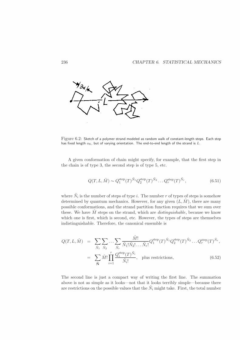
236 CHAPTER 6. STATISTICAL MECHANICS
Figure 6.2: Sketch of a polymer strand modeled as random walk of constant-length steps. Each stephas fixed length aK, but of varying orientation. The end-to-end length of the strand is L.
A given conformation of chain might specify, for example, that the first step inthe chain is of type 3, the second step is of type 5, etc.
Q(T,L, M ) ∼ Qstep1 (T )N1Qstep
2 (T )N2 . . . Qstepr (T )Nr , (6.51)
where Ni is the number of steps of type i. The number r of types of steps is somehowdetermined by quantum mechanics. However, for any given (L, M ), there are manypossible conformations, and the strand partition function requires that we sum overthese. We have M steps on the strand, which are distinguishable, because we knowwhich one is first, which is second, etc. However, the types of steps are themselvesindistinguishable. Therefore, the canonical ensemble is
Q(T,L, M ) =∑
N1
∑
N2
. . .∑
Nr
M !
N1!N2! . . . Nr!Qstep
1 (T )N1Qstep2 (T )N2 . . . Qstep
r (T )Nr ,
=∑
N
M !r∏
i=1
Qstepi (T )Ni
Ni!, plus restrictions, (6.52)
The second line is just a compact way of writing the first line. The summationabove is not as simple as it looks—not that it looks terribly simple—because thereare restrictions on the possible values that the Ni might take. First, the total number
6.6. ELASTIC STRAND 237
of steps must be M , and second, their lengths in the z direction must add up to L
r∑
i=1
Ni = M (6.53)
r∑
i=1
Nili = L. (6.54)
It is worth thinking about Eqs. (6.52)–(6.54), and understanding what each part is.The equation is basically a generalization of Eqn. (6.40), which accounts for the factthat the positions of the steps are distinguishable, and that they are connected ina certain way. We can formally include the restrictions by using a Kronecker deltafunction
δ(i, j) :=
1, if i = j0, otherwise
(6.55)
and write (6.52) as
Q(T,L, M ) =∑
N
M !δ
(
M,
r∑
k=1
Nk
)r∏
i=1
δ
(
L,
r∑
k=1
Nklk
)
Qstepi (T )Ni
Ni!,(6.56)
Including the restrictions represented by the delta functions δ(, ) is difficult, and it isprecisely here where passing to the grand canonical ensemble makes the calculationpossible. Recall that passing from the canonical ensemble Q to the grand canonicalensemble ∆, Eqn. (6.46), means summing over all possible lengths2
∆(T,T , M) :=
∫
LQ(T,L, M ) exp
[ T LkBT
]
dL
=
∫
L
∑
N
M !δ
(
M,
r∑
k=1
Nk
)
×
r∏
i=1
δ
(
L,r∑
k=1
Nklk
)
Qstepi (T )Ni
Ni!exp
[ T LkBT
]
dL (6.57)
2Note that we had to make two slight adjustments here. Quantum mechanics dictates that thepossible lengths L are not continuous but discrete. Hence, the integral over L should actually bea sum. However, since we ignore these quantum complexities, we use an integral and treat the
Kronecker delta function δ(
L,∑rk=1 Nklk
)
as a Dirac delta function δ(
L−∑rk=1 Nklk
)
.
238 CHAPTER 6. STATISTICAL MECHANICS
We can now perform the integration over L by making use of the delta function
∆(T,T , M) =∑
~N
M !
r∏
i=1
δ
(
M,
r∑
k=1
Nk
)
Qstepi (T )Ni
Ni!exp
[
T∑r
j=1 Nj lj
kBT
]
=∑
~N
M !
r∏
i=1
δ
(
M,
r∑
k=1
Nk
)
Qstepi (T )Ni
Ni!
r∏
j=1
exp
[
T NjljkBT
]
=∑
~N
M !
r∏
i=1
δ
(
M,
r∑
k=1
Nk
)[
Qstepi (T ) exp
(T likBT
)]Ni
Ni!. (6.58)
We can exploit the multinomial theorem (§A.8.2) to solve this summation
∆(T,T , M ) =
[r∑
i=1
Qstepi (T ) exp
( T likBT
)]M
. (6.59)
Next, we assume (1) that there is a large number of kinds of steps: r ≫ 1, (2) thatthe difference in their projected lengths li is very small from one kind to the next,relative to the longest possible length aK: li+1 − li ≪ aK, and (3) that the partitionfunction for a step is independent of its orientation (the environment is isotropic):Qstep
1 (T ) = Qstep2 (T ) = . . . = Qstep
r (T ) ≡ Qstep(T ). Then we can approximate thesum as an integral
r∑
i=1
Qstepi (T ) exp
( T likBT
)
= Qstep(T )r∑
i=1
exp
( T likBT
)
∼= Qstep(T )
∫ +aK
−aKexp
( T lkBT
)
rdl
2aK
= Qstep(T ) rkBT
2T aKexp
( T lkBT
)∣∣∣∣
+aK
l=−aK
= Qstep(T )rkBT
T aKsinh
(T aKkBT
)
(6.60)
When we insert Eqn. (6.60) into Eqn. (6.59) we obtain our final expression for thegrand canonical partition function ∆(T,T , M ) for a random-walk chain with Msteps under tension T
∆(T,T , M) =
[
Qstep(T )rkBT
T aKsinh
(T aKkBT
)]M
. (6.61)
6.7. FLUCTUATIONS 239
When we insert this result into Eqn. (6.46) we obtain the fundamental relation
G
MkBT= − log
[
rQstep(T )kBT
T aKsinh
(T aKkBT
)]
. (6.62)
This fundamental relation was first introduced in Eqn. (3.126). That expression,however, has replaced the step partition function Qstep(T ) in favor of the heat ca-pacity. Taking the appropriate derivative to find the length, leads to a tension-length equation of state with a form shown in Figure 6.3, and is called the inverseLangevin force law. We can see from this figure, that the results are qualitativelyvery reasonable; at low extensions, the tension rises linearly with stretching, and asthe length gets stretched to its maximum, the tension becomes very large.
However, this expression does not describe the force-extension relation for thestretching of a DNA segment particularly well. The reason for the discrepancy isour assumption that each step is independent. Even a rather large segment of DNAhas an end-to-end length comparable to its persistence length aK/2. Therefore, thisderivation needs modification, which has been done by Fixman and Kovacs [79].The (approximate) result is called the worm-like chain [57], which was introducedin Eqn. (2.85). If the strand is not greatly extended, the initial part of the force lawcurve is linear, with a slope of 3. The resulting approximate expression is called theGaussian force law.
6.7 Fluctuations
Macroscopic thermodynamic properties, such as energy, temperature, pressure, etc.are averages of fluctuating quantities. Not only does statistical mechanics providea way to predict these average quantities, it can also tell us the magnitude of thefluctuations around the averages. Why are fluctuations important? Well, for rela-tively large systems (say approximately 1023 molecules), fluctuations are importantnear the critical point. Also, for small systems, the fluctuations can become as largeas the averages themselves. Therefore, if we are designing tiny labs on a siliconchip, the data that we take will inherently have fluctuations, which make it difficultto estimate model parameters. Biological systems are typically composed of manysmall subsystems where fluctuations can also dominate. In this section we show howto estimate the size of fluctuations.
To estimate the size of fluctuations, we use the probability for a system to be ina particular micro-state. For a closed system, the postulates tell us the probabilityof a system being in a particular micro-state. By dividing a closed system into asubsystem and a bath, we also derived the probabilities for particular microstates.These results are summarized in Table 6.1. A system, say, held at fixed temperature,
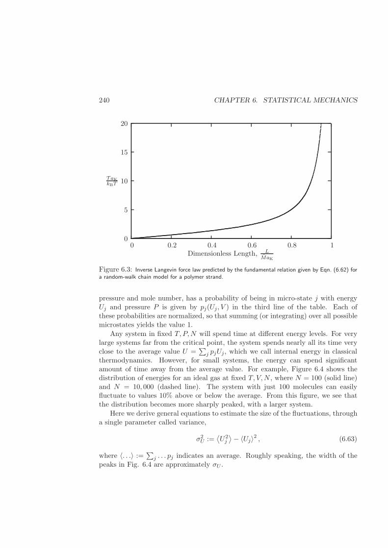
240 CHAPTER 6. STATISTICAL MECHANICS
0
5
10
15
20
0 0.2 0.4 0.6 0.8 1
T aKkBT
Dimensionless Length, LMaK
Figure 6.3: Inverse Langevin force law predicted by the fundamental relation given by Eqn. (6.62) fora random-walk chain model for a polymer strand.
pressure and mole number, has a probability of being in micro-state j with energyUj and pressure P is given by pj(Uj , V ) in the third line of the table. Each ofthese probabilities are normalized, so that summing (or integrating) over all possiblemicrostates yields the value 1.
Any system in fixed T, P,N will spend time at different energy levels. For verylarge systems far from the critical point, the system spends nearly all its time veryclose to the average value U =
∑
j pjUj, which we call internal energy in classicalthermodynamics. However, for small systems, the energy can spend significantamount of time away from the average value. For example, Figure 6.4 shows thedistribution of energies for an ideal gas at fixed T, V,N , where N = 100 (solid line)and N = 10, 000 (dashed line). The system with just 100 molecules can easilyfluctuate to values 10% above or below the average. From this figure, we see thatthe distribution becomes more sharply peaked, with a larger system.
Here we derive general equations to estimate the size of the fluctuations, througha single parameter called variance,
σ2U :=⟨U2j
⟩− 〈Uj〉2 , (6.63)
where 〈. . .〉 := ∑
j . . . pj indicates an average. Roughly speaking, the width of thepeaks in Fig. 6.4 are approximately σU .
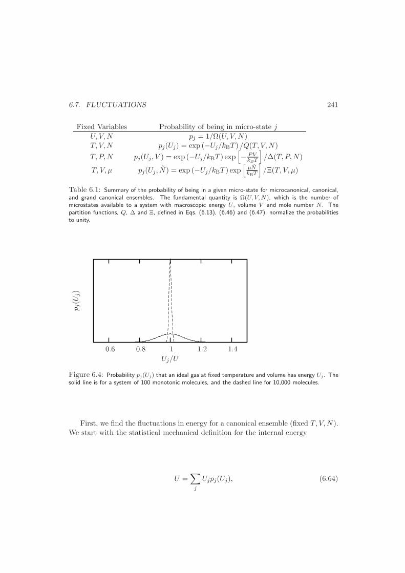
6.7. FLUCTUATIONS 241
Fixed Variables Probability of being in micro-state j
U, V,N pj = 1/Ω(U, V,N)T, V,N pj(Uj) = exp (−Uj/kBT ) /Q(T, V,N)
T, P,N pj(Uj , V ) = exp (−Uj/kBT ) exp[
− PVkBT
]
/∆(T, P,N)
T, V, µ pj(Uj, N ) = exp (−Uj/kBT ) exp[µNkBT
]
/Ξ(T, V, µ)
Table 6.1: Summary of the probability of being in a given micro-state for microcanonical, canonical,and grand canonical ensembles. The fundamental quantity is Ω(U, V,N), which is the number ofmicrostates available to a system with macroscopic energy U , volume V and mole number N . Thepartition functions, Q, ∆ and Ξ, defined in Eqs. (6.13), (6.46) and (6.47), normalize the probabilitiesto unity.
Uj/U
pj(U
j)
1.41.210.80.6
Figure 6.4: Probability pj(Uj) that an ideal gas at fixed temperature and volume has energy Uj . Thesolid line is for a system of 100 monotonic molecules, and the dashed line for 10,000 molecules.
First, we find the fluctuations in energy for a canonical ensemble (fixed T, V,N).We start with the statistical mechanical definition for the internal energy
U =∑
j
Ujpj(Uj), (6.64)
242 CHAPTER 6. STATISTICAL MECHANICS
and take the derivative of each side with respect to temperature(∂U
∂T
)
V,N
=∑
j
Uj
(∂pj∂T
)
V,N
CV =∑
j
Uj
[
UjkBT 2
pj −pjQ
(∂Q
∂T
)
V,N
]
=〈U2
j 〉kBT 2
− 〈Uj〉Q
(∂Q
∂T
)
V,N
=〈U2
j 〉kBT 2
− 〈Uj〉∑
j
UjkBT 2
exp (−Uj/kBT )Q
=〈U2
j 〉kBT 2
− 〈Uj〉2kBT 2
=σ2UkBT 2
. (6.65)
To obtain the second line, we used the canonical probability distribution from Table6.1, and the definition of the constant-volume heat capacity. To get to the thirdline, we used the definition of an average. The fourth line arises from the definitionof the canonical partition function, Table 6.2, and the fifth line uses the probabilitydistribution again. The last line comes from the definition for variance, Eqn. (6.63).The result given in Eqn.(6.65) is remarkable; as molecules collide against one anotherin a fluid they give rise to fluctuations of the energy. The heat capacity of a fluid isa measure of those fluctuations; Eqn. (6.65) gives a precise correspondence betweenthe variance of such fluctuations and the heat capacity.
Note the size dependence of the final result
σU (T, V,N)
〈U〉 =
√
kBT 2CV〈U〉 =
1√
N
√
RT 2cV〈u〉
︸ ︷︷ ︸
sizeindependent
. (6.66)
We introduced the notation here for the deviation σ, where the subscript indicatesthe fluctuating quantity, and the arguments which variables are held constant. Theleft side here is dimensionless, so it gives the relative magnitude of the fluctuations.Hence, the relative width of the distribution shrinks with the square root of systemsize (number of molecules).
Example 6.7.1 What are the relative fluctuations of internal energy in 1µl of asimple ideal gas at standard temperature and pressure?
6.7. FLUCTUATIONS 243
Solution: A simple ideal gas has average specific internal energy 〈u〉 = 32RT .
Hence, it has specific constant-volume heat capacity cv = 32R. We can use
Eqn. (6.66) to estimate the relative energy fluctuations as
σU〈U〉 =
√2
3N
=
√
2RT
3PV NA
=
√
2(298K)(0.0802l · atm/mol ·K)
3(1atm)(10−6l)(6.023× 10²³mol−1)
∼= 5× 10⁻⁹. (6.67)
Hence, even for a box of only one microliter, the fluctuations are in the 8thdecimal place, and typically insignificant.
2
Similarly, one can show that
σN (T, V, µ)
〈N〉 =
√
kBTκTV
.
σV (T, P,N)
〈V 〉 =
√
kBTκTV
. (6.68)
These last two results show why fluctuations are large near the critical point. Recallfrom §4.2.1 that the spinodal curve is where
(∂P∂v
)
T= 0, or where κT = ∞. The
critical point is where the spinodal curve is at a maximum, so near this point, thefluctuations in volume (or density) and in mole numbers become extremely large,even for large systems. This result in fact explains why the heat capacity of a fluiddiverges as the critical point is approached.
Example 6.7.2 Bustamante, et al. [11] have measured the length of a segment ofDNA under tension isothermally using an optical trap. At low tensions, they observelarge fluctuations in the length, and it takes some time to find the average length.What is the size of the fluctuations in length for an isothermal polymer strand heldunder tension?
Solution: Using our usual mapping, we can use the results above on volumefluctuations with the substitutions: V → L, −P → T , and N → M . The length
244 CHAPTER 6. STATISTICAL MECHANICS
as a function of tension is found from the free energy of the strand, Eqn. (6.62)
〈L〉MaK
= − 1
MaK
(∂G
∂T
)
T,M
= coth
(T aKkBT
)
− kBT
T aK, (6.69)
which is the inverse Langevin force law plotted in Figure 6.3. By taking thederivative of this expression, and dividing the result by the equation itself, weobtain the isothermal “compressibility”
κT :=1
〈L〉
(∂〈L〉∂T
)
T,M
=1
T
kBTT aK
− T aKkBT
csch2(
T aKkBT
)
coth(
T aKkBT
)
− kBTT aK
. (6.70)
Now we can use our results from this section, Eqn. (6.68), to find the relativemagnitude of the fluctuations in length of the strand
σL(T, T , M)
〈L〉 =
√
kBTκT〈L〉
=1√
M
√
x−2 − csch2(x)
coth(x)− x−1, (6.71)
where x := T aKkBT
is the dimensionless tension. There are two things worthwhileto note about this result. First, we see again that the relative magnitudedepends inversely upon the square root of the number of segments in the chain,which is another specific example of the general result (the simple ideal gas wasthe first). Secondly, we see that there is a tension-dependent part that can makethe fluctuations very large, even for long chains. To illustrate the importanceof this second term, we plot it versus dimensionless tension in Figure 6.5
In accord with observations, we see that the relative fluctuations are muchlarger for smaller tensions. The result is not surprising, since the average lengthgoes to zero for no tension, but the fluctuations stay finite. 2
6.8 Summary
In this chapter we showed how to relate atomic interactions to thermodynamicproperties. In theory, the connection arises from two simple statistical mechanicalpostulates
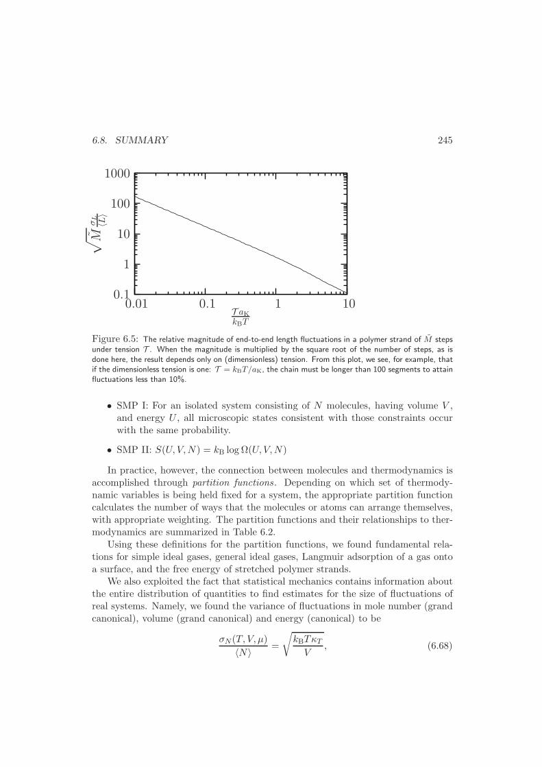
6.8. SUMMARY 245
T aKkBT
√
MσL 〈L〉
1010.10.01
1000
100
10
1
0.1
Figure 6.5: The relative magnitude of end-to-end length fluctuations in a polymer strand of M stepsunder tension T . When the magnitude is multiplied by the square root of the number of steps, as isdone here, the result depends only on (dimensionless) tension. From this plot, we see, for example, thatif the dimensionless tension is one: T = kBT/aK, the chain must be longer than 100 segments to attainfluctuations less than 10%.
• SMP I: For an isolated system consisting of N molecules, having volume V ,and energy U , all microscopic states consistent with those constraints occurwith the same probability.
• SMP II: S(U, V,N) = kB log Ω(U, V,N)
In practice, however, the connection between molecules and thermodynamics isaccomplished through partition functions. Depending on which set of thermody-namic variables is being held fixed for a system, the appropriate partition functioncalculates the number of ways that the molecules or atoms can arrange themselves,with appropriate weighting. The partition functions and their relationships to ther-modynamics are summarized in Table 6.2.
Using these definitions for the partition functions, we found fundamental rela-tions for simple ideal gases, general ideal gases, Langmuir adsorption of a gas ontoa surface, and the free energy of stretched polymer strands.
We also exploited the fact that statistical mechanics contains information aboutthe entire distribution of quantities to find estimates for the size of fluctuations ofreal systems. Namely, we found the variance of fluctuations in mole number (grandcanonical), volume (grand canonical) and energy (canonical) to be
σN (T, V, µ)
〈N〉 =
√
kBTκTV
, (6.68)
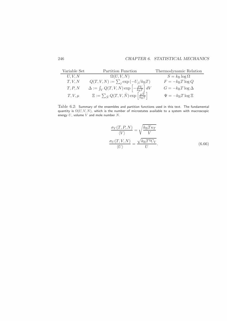
246 CHAPTER 6. STATISTICAL MECHANICS
Variable Set Partition Function Thermodynamic Relation
U, V,N Ω(U, V,N) S = kB log ΩT, V,N Q(T, V,N) :=
∑
j exp (−Uj/kBT ) F = −kBT logQ
T,P,N ∆ :=∫
V Q(T, V,N) exp[
− PVkBT
]
dV G = −kBT log ∆
T, V, µ Ξ :=∑
N Q(T, V, N) exp[µNkBT
]
Ψ = −kBT log Ξ
Table 6.2: Summary of the ensembles and partition functions used in this text. The fundamentalquantity is Ω(U, V,N), which is the number of microstates available to a system with macroscopicenergy U , volume V and mole number N .
σV (T, P,N)
〈V 〉 =
√
kBTκTV
σU (T, V,N)
〈U〉 =
√
kBT 2CVU
. (6.66)
6.9. EXERCISES 247
6.9 Exercises
6.2.A. Consider a simple binomial coefficient of the form Should this read“large M” instead of“large N1”. Also, anexpression for whatis being asked to bederived? Ω? JDS07/11/2007
Ω =(N1 +N2)!
N1!N2!(6.72)
Find the value of N1 for which Ω is a maximum, for fixedM = N1+N2 . If we use anasterisk to denote this “maximum” distribution, derive an approximate (first-order)expression in terms of N1 and N∗
1 . Use this expression to show that, for large valuesof N1, the binomial coefficient is strongly peaked around N∗
1 .
6.3.A. Verify that the first line of Eqn. (6.39)
U
NRT= −T
(∂
∂T
F
NRT
)
V,N
is generally true.
6.3.B. Show that the canonical partition function derived for a mixture of non-interacting polyatomic gases, Eqn. (6.35) leads to the fundamental relation for amixture of general ideal gases, §7.1.6.3.C. Show that, for an ideal gas comprising N molecules at temperature T , thenumber of molecules having velocity between v and v + dv is given by
4πN
(m
2πkBT
)3/2
exp
[
− mv2
2kBT
]
v2dv, (6.73)
where m is the mass of each molecule.
6.3.D. Non-ideal gases are often described by a mechanical equation of state of theform
P
ρkBT= 1 +Bρ+O(ρ2), (6.74)
where B is a so-called second virial coefficient that depends only on temperature.Show that, for a system of spherical molecules where each pair of molecules interactsthrough a potential energy function denoted by Γ(r), the second virial coefficient isgiven by
B = 2π
∫ ∞
0
1− exp
[
−Γ(r)
kBT
]
r2dr, (6.75)
where r denotes the distance between a pair of molecules.
248 CHAPTER 6. STATISTICAL MECHANICS
Hint : use a grand-canonical ensemble, and begin by showing that the partitionfunction can be written as
Ξ = 1 +
∞∑
N=1
ZN (V, T )
N !zN , (6.76)
where z is an activity defined as z = Q1
V eµ/kBT , and Q1 is a single-particle partition
function, i.e., Q1 := V/Λ3. Note that the N-particle canonical ensemble partition
function can be written as QN = 1N !
(Q1
V
)NZN , where
ZN =
∫
Vexp
[
−Upot(~rN )
kBT
]
d~rN (6.77)
is the so-called configurational integral and Upot(~rN ) is the potential energy of the
system, which in this case is given by Upot(~rN ) = 1
2
∑Ni
∑Nj Γij(rij). Next show
that the pressure can be written in the following form
P
kBT=
∞∑
j=1
bj(T )zj , (6.78)
where the bj(T ) are temperature dependent coefficients given by
b1 =1
VZ1 (6.79)
b2 =1
2V(Z2 − Z2
1 ) (6.80)
b3 =1
6V(Z3 − 3Z1Z2 − 2Z3
1 ) (6.81)
... (6.82)
The series for the pressure can then be inverted by postulating that
z =∞∑
i=1
aiρi , (6.83)
substituting z from Equation (6.83) into a series for the density, which can be derivedfrom Equation (6.78), and matching the coefficients corresponding to each power ofz. This procedure should allow you to show that
B(T ) = −b2(T ) = − 1
V(Z2 − Z2
1 ), (6.84)
6.9. EXERCISES 249
where
Z1 =
∫
Vdr1 (6.85)
Z2 =
∫ ∫
Vexp
[
−Γ(r)
kBT
]
dr1dr2 . (6.86)
6.3.E. Quantum mechanics tells us the energy of a diatomic molecule. There arethree contributions: electronic, vibrational, and rotational. If we neglect dissociationof the molecule into two atoms, then the electronic energy ε0 is a constant. Hence,the microstate of the molecule can be described by two integers ν and K, where
EνK = ε0 + hω
(
ν +1
2
)
+ h2K(K + 1)
2I; ν,K = 0, 1, 2, . . . (6.87)
where EνK is the energy of the molecule in that microstate, h is Planck’s constant,ω is the vibrational frequency (measurable from IR), and I is the moment of inertiaof the molecule. Note that this result is only for an asymmetric diatomic molecule,and that the rotational energy has degeneracy 2K+1, meaning that there are 2K+1distinct microstates with the same rotational energy.
Find the molecule partition function for this asymmetric diatomic molecule.Approximate the sum for the vibrational component as an integral. State explicitlywhen this approximation is valid. The vibrational part can be summed analytically.
6.4.A Derive the Langmuir adsorption fundamental relation for the simultaneous ad-sorption of two types of molecules A and B. In other words, find F (T, Ms, NA, NB)for NA molecules of type A and NB molecules of type B adsorbed on a surface withMs sites. Make a detailed comparison between your results and Eqn. (3.130).
6.4.B Consider surface adsorption if the molecules in the Langmuir adsorption haveinternal degrees of freedom, such that
Etot(~rN , ~pN , ~RN ) =
N∑
i=1
Emol(~ri, ~pi, ~Ri), (6.88)
where ~Ri is the vector of internal conformations, like we used for a general ideal gas(see Eqn. (6.29)). Derive the new fundamental relation.
6.4.C Derive the partition function and fundamental relation for hemoglobin, Eqn. (3.132).
6.5.A. Derive the expressions for the grand canonical ensemble, Eqs. (6.46–6.47).Follow the same procedure as we did in §6.2, however, now let molecules exchangebetween the bath and the subsystem to obtain Ψ, or the volume to obtain G.
250 CHAPTER 6. STATISTICAL MECHANICS
6.5.B. Derive an expression for the grand-canonical ensemble partition function ofa two-component system. Could the
6.5.B be madespecific (clearer)?JDS 07/11/2007
6.5.C. Derive an expression for the partition function in the isobaric-isothermal(NPT ) ensemble. What is the natural thermodynamic potential for this ensem-ble? How is this potential related to the partition function? Can you propose anygeneral rules to relate an arbitrary partition function to its “natural” thermody-namic potential?
6.5.D. Show that the partition function Ξ′(N1, µ2, U, P ) for a two-component systemdefined by constant U , constant P , constant number of particles for component oneand constant chemical potential for component two is given by
Ξ′ =∑
exp
(
−µN2
kBT
)
exp
(
− PV
kBT
)
. (6.89)
Derive the natural thermodynamic potential for this ensemble.Should this µ be µ2?JDS 07/11/2007
6.6.A A polymer chain is placed in an electric field. Each segment of the chain hasa dipole moment, so it has energy ~E · ~uα, where ~E is the electric field, and ~u is aunit vector describing the orientation of the segment. Unlike the derivation in §6.6,the step partition function now depends on i, with an isotropic part, and an energyfrom the field
Qstepi (T ) = Q0(T ) exp
(
− ~E · ~uα)
.
The ends of the chain are pulled apart with tension ~T , which is a vector. Findan expression for the end-to-end vector of the chain ~L as a function of temperatureT , number of segments M , tension ~T and electric field ~E. For convenience, put thetension vector ~T along the z-axis so that ~T · ~li = T aKui,z.6.6.B Show how to obtain Eqn. (3.126) from (6.62). What is the heat capacity?
6.6.C Consider a generalization to the Langmuir adsorption model, where multiplemolecules can be adsorbed on a single site. We assume that molecules adsorbedon adjacent sites do not interact energetically. However, the molecules on a singlesite do interact, so that we write q1(T ) as the partition function of a site with onemolecule adsorbed, q2(T ) for two molecules, etc.
a. Show how the canonical partition function for this problem is similar to thatfor the elastic strand, Eqn. (6.52).
b. Now pass to the grand canonical partition function Ξ, and find an expressionfor the fraction of adsorbed molecules θ := N/Ms.
c. From this result, one can derive the Brunauer-Emmett-Teller model, Eqn.(3.117), by making certain assumptions. One assumes that q1 = qsite(T ), q2 =qsite(T )/c, q3 = qsite(T )/c
2, q4 = qsite(T )/c3, and so on. Show how this assumption
6.9. EXERCISES 251
leads to the B.E.T. model. What is c? Note that it is not necessary to approximatethe sums as integrals here.
6.6.D In §3.7.2, we found the tension-temperature phase diagram for unzipping DNAby pulling. Here we consider just one step in the statistical mechanical derivationof that fundamental relation, Eqn. (3.102). We begin with the canonical partitionfunction Q(T,L, M ), where T is temperature, L is the distance between the two endsof the two different strands being pulled, and M is the total number of base pairs onthe DNA. Just like the zipper model, we assume that the base pairs are energeticallyindependent, so that we can assume a partition function qa(T ) for attached bases,and a partition function qu(T ) for unattached bases. Additionally, nb consecutive,unattached base pairs can form a Kuhn step having orientation i, with partitionfunction qstepj (T ). So, the canonical partition function can be written
Q =
M∑
N=0
qa(T )Nqu(T )
M−N∑
I1
. . .∑
Ir
[
2(M − N)
nb
]
!
r∏
j=1
qstepj (T )Ij
Ij !
where N is the number of attached base pairs, which we sum over. This expressionalso contains a sum over possible orientations of the Kuhn steps, where Ij is thenumber of steps with orientation j. The summation has the following two restrictions
∑
j
Ij =2(M − N)
nb, (R1)
∑
j
ljIj = L, (R2),
where lj is the length of a step of type j in the direction of L. From this expressionfor the canonical partition function, derive the fundamental relation, Eqn. (3.102).
6.6.E Actin is a globular protein that is contained in all species. In a cell, actinpolymerizes to form filaments that form the cytoplasmic skeleton. This problem needs
clarification.Students areprobably not awarethat fiberpolymerizes anddepolymerizes. Also,are they basicallybeing asked to findthe distribution offiber lengths? JDS07/11/2007
In this problem you are required to find the partition function that describesthe polymerization of actin in a cell. Also give an expression for the mean lengthof the actin polymer. Assume total number of actin molecules Ntot is large. Let Eidenote the energy of a filament with i units and Li denote its length. (Li = L0 ∗ i,L0 = length of a single unit and i = number of units.) The cell can be treated asan isothermal system.
6.6.F. Imagine a single polymer chain, oriented more or less in a straight line. Alongthe backbone of this chain are arranged evenly spaced side groups each of which actsas a dipole:
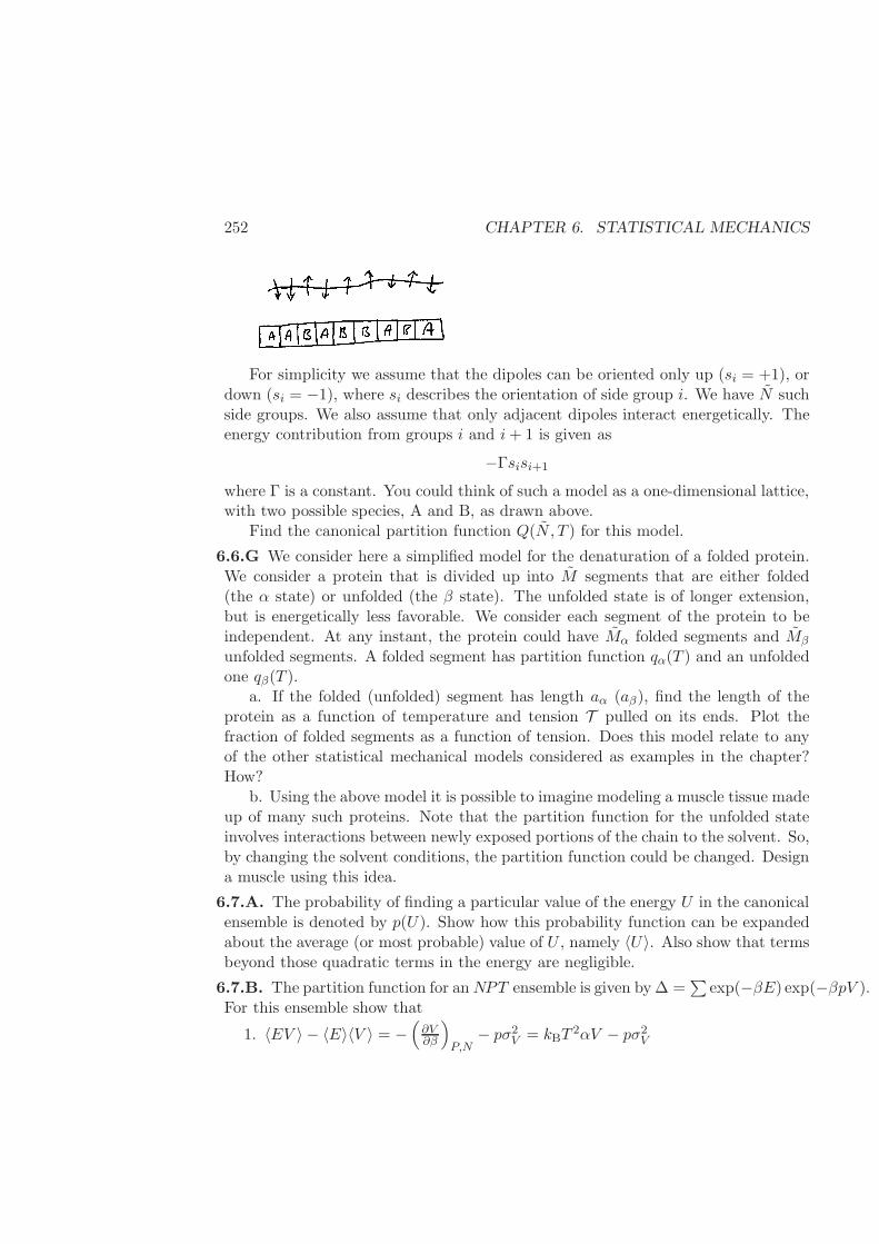
252 CHAPTER 6. STATISTICAL MECHANICS
For simplicity we assume that the dipoles can be oriented only up (si = +1), ordown (si = −1), where si describes the orientation of side group i. We have N suchside groups. We also assume that only adjacent dipoles interact energetically. Theenergy contribution from groups i and i+ 1 is given as
−Γsisi+1
where Γ is a constant. You could think of such a model as a one-dimensional lattice,with two possible species, A and B, as drawn above.
Find the canonical partition function Q(N , T ) for this model.
6.6.G We consider here a simplified model for the denaturation of a folded protein.We consider a protein that is divided up into M segments that are either folded(the α state) or unfolded (the β state). The unfolded state is of longer extension,but is energetically less favorable. We consider each segment of the protein to beindependent. At any instant, the protein could have Mα folded segments and Mβ
unfolded segments. A folded segment has partition function qα(T ) and an unfoldedone qβ(T ).
a. If the folded (unfolded) segment has length aα (aβ), find the length of theprotein as a function of temperature and tension T pulled on its ends. Plot thefraction of folded segments as a function of tension. Does this model relate to anyof the other statistical mechanical models considered as examples in the chapter?How?
b. Using the above model it is possible to imagine modeling a muscle tissue madeup of many such proteins. Note that the partition function for the unfolded stateinvolves interactions between newly exposed portions of the chain to the solvent. So,by changing the solvent conditions, the partition function could be changed. Designa muscle using this idea.
6.7.A. The probability of finding a particular value of the energy U in the canonicalensemble is denoted by p(U). Show how this probability function can be expandedabout the average (or most probable) value of U , namely 〈U〉. Also show that termsbeyond those quadratic terms in the energy are negligible.
6.7.B. The partition function for anNPT ensemble is given by ∆ =∑
exp(−βE) exp(−βpV ).For this ensemble show that
1. 〈EV 〉 − 〈E〉〈V 〉 = −(∂V∂β
)
P,N− pσ2V = kBT
2αV − pσ2V
6.9. EXERCISES 253
2. 〈H2〉 − 〈H2〉 = kBT2CP .
6.7.C. Prove the fluctuation formulas given in Eqs. (6.68). The first can be foundby differentiating 〈N〉 with respect to µ in the grand canonical ensemble (T, V, µ).Similarly, differentiate the average 〈V 〉 with respect to P in the (T, P,N) ensembleto find the second.
6.7.D. Find the deviations σU (T, V,N), σN (T, V, µ), and σV (T, P,N) for a mono-tonic ideal gas. How many molecules does your system need to insure that therelative magnitude of these fluctuations is below 10−6?
6.7.E. Find the magnitude of the fluctuations in length for a worm-like chain as afunction of tension.

254 CHAPTER 6. STATISTICAL MECHANICS
Chapter 7
Molecular Interactions
I’m not sure that ρ isconsistentthroughout the text.Sometimes it is massper volume, andsometimes moles pervolume. JDS07/11/2007
Previous chapters established many relations between various thermodynamicproperties of a fluid. We have seen, for example, that the heat capacity of a fluidis always positive. We have also shown that the thermal, mechanical and chemicalequations of state of must be mutually consistent (i.e., they must satisfy the Gibbs-Duhem equation). In the previous chapter, we showed how statistical mechanicscan be used to derive fundamental thermodynamic relations from simple models ofmolecular interactions. In this chapter we discuss in greater detail important molec-ular interactions, and their relative magnitudes. Specific mathematical expressionstaken from physical chemistry are used to estimate when interactions are important,and how they might influence thermodynamic quantities.
The equations of state and the transport properties of gases, liquids and solidsare intimately related to the forces between the molecules. The methods of statis-tical mechanics provide a connection between these forces and measurable thermo-dynamic properties. An introduction to statistical mechanics was presented in theprevious chapter. Here we merely discuss the nature and the origin of intermolecularforces.
7.1 Ideal Gases
As a starting point, we consider a gas with no intermolecular forces, and no internaldegrees of freedom. Such a fluid is called a simple ideal gas, and was derived in§6.3.1. The pressure exerted by N moles of an ideal gas confined to a volume Vtherefore arises as a result of the sum of the momentum (or kinetic energy) of each
255
256 CHAPTER 7. MOLECULAR INTERACTIONS
particle, and it is given by the familiar equation
P =NRT
V. (7.1)
The internal energy is also a sum of the contribution of each particle, and is
U = cNRT. (7.2)
A fundamental entropy expression for the ideal gas was given in Chapter 2 as
S = Ns0 +NR log
[(U
Nu0
)c V
Nv0
]
, (7.3)
where s0, u0 and v0 are constants of integration corresponding to the reference-statemolar entropy, energy and volume of the gas in an ideal state.
Since the molecules of an ideal gas do not interact with each other, the energyof a mixture of ideal gases can be written as
U =
(r∑
i
Nici
)
RT, (7.4)
and an entropy equation of state for a mixture of ideal gases may be written
S =r∑
i
Nisi0 +r∑
i
(Nici)R logT
T0+
r∑
i
NiR log
(V
Niv0
)
. (7.5)
In other words, the entropy of an ideal gas mixture is given by the sum of theentropies that each component would have if it, alone, were to occupy all of volume Vat temperature T . This last statement is also known as Gibbs’ theorem. From theselast two expressions it is straightforward to write down a fundamental Helmholtzrelation for a mixture of ideal gases F (T, V, Ni) := U − TS. Next we considerwhen molecules do interact.
7.2 Intermolecular Interactions
7.2.1 Significance of “kBT”
The product of the Boltzmann constant and the temperature, known affectionatelyas “kBT”, is often used as a measure of the strength of an intermolecular interaction.Indeed, it is not uncommon to attend lectures in which entire hypotheses and dis-cussions are cast in terms of multiples of kBT . The thought is that if an interaction
7.2. INTERMOLECULAR INTERACTIONS 257
energy exceeds kBT , it will overcome the disorganizing effects of thermal motion.Or, on the other hand, if an interaction energy is many times that of kBT , thermalmotion will rarely overcome it.
The significance of kBT can be illustrated by analyzing the cohesive energyresponsible for condensing a gas into a liquid. This cohesive energy is approximatelyequal to the latent enthalpy of vaporization, ∆hvap. Loosely speaking, the insertionof one molecule into a liquid phase requires that 12 nearest neighbors be displacedin order to create a cavity. This would necessitate that six nearest neighbor “bonds”be broken. If the energy of two molecules at near contact is comparable to ǫ, thenthe energy required to carry out this process is 6ǫ.
Experimental data for numerous substances [46, p.281] suggest the followingrelation between the enthalpy of vaporization and the boiling temperature TB
∆hvap
TB≈ 80
J
K ·mol∼= 9.6R. (7.6)
Eqn. (7.6) is known as Trouton’s law. The quantity on the right is approximatelyequal to 9kB per molecule. We can therefore infer that if the energy of interactionbetween two molecules exceeds about 3
2kBT , then it is strong enough to result incondensation into a liquid or solid. This simple analysis helps explain why kBT isused as the “unit” with which one gauges the strength of intermolecular interactions.So, it is useful to keep in mind that kBT ∼= 4.14 × 10⁻²¹J ∼= 2.5kJ/mol at roomtemperature.
7.2.2 Interactions at Long Distances
Coulombic Forces
The beginning point of the inter-atomic or intermolecular interactions in which weare interested resides in the attractions or repulsions between charged subatomicparticles, namely electrons and protons. The energy of interaction Γij between twopoint charges qi and qj in vacuo is given by Coulomb’s law
Γij =qiqj4πǫ0r
, point charges, (7.7)
where r is the distance between the particles, and ǫ0 is the dielectric permittivity ofvacuum, namely ǫ0 = 8.8542 × 10⁻¹² C2J−1m−1. In general, the force ~Fij betweentwo particles interacting through a potential energy function Γij is given by
~Fij = −∇Γij. (7.8)
258 CHAPTER 7. MOLECULAR INTERACTIONS
Recall the definition of the vector differential operator: ∇ := ~δx∂∂x + ~δy
∂∂y + ~δz
∂∂z .
The magnitude of the force between two charges is therefore given by
| ~Fij | =qiqj
4πǫ0r2. (7.9)
Two charges of similar sign have a positive energy of interaction, thereby givingrise to a positive, repulsive force between them; two charges of opposite sign havea negative energy of interaction and they attract each other. As we shall discussbelow, Coulombic or electrostatic interactions are relatively strong and long ranged.Consider two isolated ions, Na+ and Cl−, at contact. The distance between themis the sum of their atomic radii, approximately 0.276 nm. From Eqn. (7.7), theirenergy of interaction is
Γij =−(1.602 × 10⁻¹⁹C)2
4π(8.8542 × 10⁻¹²C2J−1m−1)(0.276 × 10⁻⁹m)= −8.4× 10⁻¹⁹J, (7.10)
where e = 1.602× 10⁻¹⁹C is the elementary charge. At room temperature, this en-ergy of interaction corresponds to approximately −200kBT . This simple calculationillustrates that the energy of interaction between two ions in vacuum is comparableto that of a covalent bond (several hundred times kBT ). Furthermore, this calcula-tion shows that energy does not decay to kBT until the distance between the ionsis on the order of 0.1µm; the range of interaction is indeed long-range, particularlywhen we consider that the diameter of an ion is on the order of just a few Angstrom!A more realistic calculation of the cohesive energy of an ionic crystal must thereforetake into account contributions arising from nearest-neighbors, next-nearest neigh-bors, and so on and so forth. For a cubic lattice such as that formed by NaCl, acentral Na+ ion is surrounded by 6 surrounding Cl− at distance 0.276nm, by 12next-nearest Na+ neighbors at
√2r, eight Cl− at
√3r, etc. The cohesive energy Γc
of a NaCl crystal is therefore given by
Γc =qiqj4πǫ0r
(
6− 12√2+
8√3+ ...
)
∼= 1.748qiqj4πǫ0r
= −1.46× 10⁻¹⁸J. (7.11)
This number is higher than that predicted for a pair of ions in vacuum by a factorof 1.748; this factor appearing in Eqn. (7.11) is known as Madelung’s constant,1
and it assumes different values depending on the type of crystal lattice formed bythe ions.
1Note that this term is a geometrical correction for a specific kind of lattice, in this case NaCl.The term “Madelung’s constant” is sometimes used only for this lattice, and sometimes for anygeneral lattice, in which case a number different from 1.748 can arise.
7.2. INTERMOLECULAR INTERACTIONS 259
Permanent Dipoles
Electrostatic or Coulombic forces arise not only between charged particles (e.g.,ions), but also between neutral molecules (i.e., molecules that do not exhibit a netcharge). Consider here the case of a neutral molecule that possesses two charges ofthe same magnitude qi but opposite sign. If the distance between the two chargesis denoted by d, that molecule has a dipole moment µdi given by
µdi = qid (7.12)
Molecules such as ethanol, acetone or water have a relatively large dipole moment,because of the asymmetry in the distribution of charges (electrons and protons)within the molecule. In contrast, symmetric molecules such as methane have arelatively small, usually negligible permanent dipole moment.
The energy of interaction between two dipolar molecules depends on the distanceand the orientation between the dipoles. Figure 7.1 describes schematically ourcoordinate system for the relative position of the dipoles. If r is used to denotethe distance between the dipole centers of mass, and φ, θi and θj denote the anglesbetween these (see Figure 7.1), then it can be shown [56] that the instantaneousenergy of interaction between them is given by
Γij = −µdi µ
dj
4πǫ0r3(2 cos θi cos θj − sin θi sin θj cosφ) , permanent dipole. (7.13)
A simple analysis of Figure 7.1 suggests that two dipoles attract each other stronglywhen they are co-linear and their “directions” are opposite. They repel each otherwhen they are co-linear and their directions are the same. These observations are
consistent with Eqn. (7.13); the energy in the first case is Γij = − µdi µdj
2πǫ0r3, whereas
in the latter case it is Γij =µdi µ
dj
2πǫ0r3. It is interesting to note that, when the origin
of the interactions between two neutral, dipolar molecules is electrostatic, theirinstantaneous energy decays as the third power of the distance between them (asopposed to the inverse power).
In an actual fluid the relative orientation between any two dipolar moleculesis not constant, but fluctuates incessantly as the molecules travel through space.It is then useful to calculate an average energy of interaction between two suchmolecules. The average is determined by considering all possible orientations be-tween the dipoles, and weighting more heavily (according to their Boltzmann factor,see Table 6.1) those configurations that have a lower energy. The result of this pro-cedure is an average energy given, to leading order, by [56]
〈Γij〉 =−2(µdi )
2(µdj )2
(4πǫ0)2kBTr6+ . . . . (7.14)
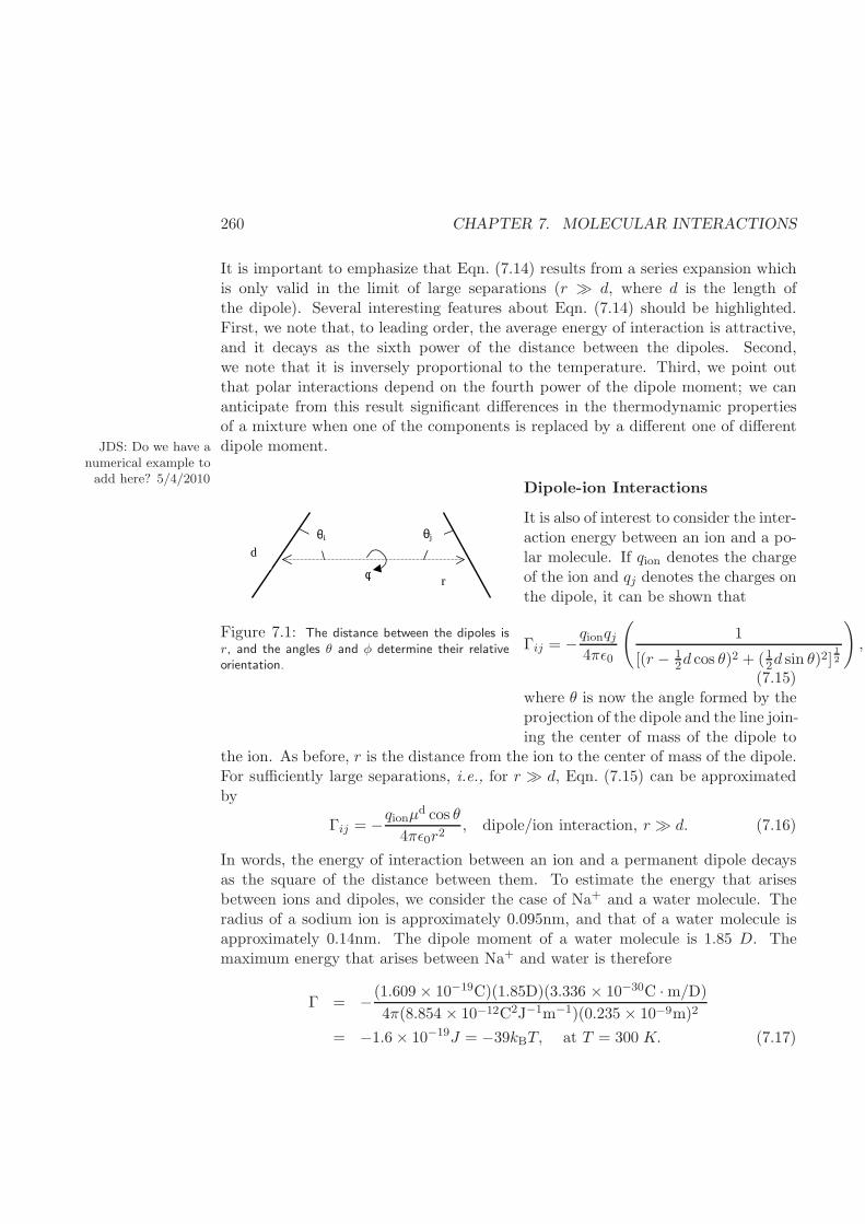
260 CHAPTER 7. MOLECULAR INTERACTIONS
It is important to emphasize that Eqn. (7.14) results from a series expansion whichis only valid in the limit of large separations (r ≫ d, where d is the length ofthe dipole). Several interesting features about Eqn. (7.14) should be highlighted.First, we note that, to leading order, the average energy of interaction is attractive,and it decays as the sixth power of the distance between the dipoles. Second,we note that it is inversely proportional to the temperature. Third, we point outthat polar interactions depend on the fourth power of the dipole moment; we cananticipate from this result significant differences in the thermodynamic propertiesof a mixture when one of the components is replaced by a different one of differentdipole moment.JDS: Do we have a
numerical example toadd here? 5/4/2010
d
θj
φ
θi
r
Figure 7.1: The distance between the dipoles isr, and the angles θ and φ determine their relativeorientation.
Dipole-ion Interactions
It is also of interest to consider the inter-action energy between an ion and a po-lar molecule. If qion denotes the chargeof the ion and qj denotes the charges onthe dipole, it can be shown that
Γij = −qionqj4πǫ0
(
1
[(r − 12d cos θ)
2 + (12d sin θ)2]
12
)
,
(7.15)where θ is now the angle formed by theprojection of the dipole and the line join-ing the center of mass of the dipole to
the ion. As before, r is the distance from the ion to the center of mass of the dipole.For sufficiently large separations, i.e., for r ≫ d, Eqn. (7.15) can be approximatedby
Γij = −qionµd cos θ
4πǫ0r2, dipole/ion interaction, r ≫ d. (7.16)
In words, the energy of interaction between an ion and a permanent dipole decaysas the square of the distance between them. To estimate the energy that arisesbetween ions and dipoles, we consider the case of Na+ and a water molecule. Theradius of a sodium ion is approximately 0.095nm, and that of a water molecule isapproximately 0.14nm. The dipole moment of a water molecule is 1.85 D. Themaximum energy that arises between Na+ and water is therefore
Γ = −(1.609 × 10⁻¹⁹C)(1.85D)(3.336 × 10⁻³⁰C ·m/D)
4π(8.854 × 10⁻¹²C2J−1m−1)(0.235 × 10⁻⁹m)2
= −1.6× 10⁻¹⁹J = −39kBT, at T = 300 K. (7.17)
7.2. INTERMOLECULAR INTERACTIONS 261
Note that we used the dipole moment of water in Debye (D) from Table 7.2, andthe conversion factor to Coulomb-meters. This energy is relatively large, and isresponsible for the so-called solvation or hydration of ions in highly polar solventssuch as water. A cation such as sodium in aqueous solution at room temperatureusually has between 4 and 5 water molecules “bound” to it; that is, the hydrationnumber of sodium in water is between 4 and 5. While these water molecules arefree to exchange with other molecules further away, they do so at a relatively slowrate. The bare radius of a sodium ion is 0.095nm, but that of the hydrated ion ismuch larger; the so-called hydration radius of sodium is approximately 0.36nm. Incontrast, the hydration number of a negatively charged chlorine anion is unity.
Molecules can also have quadrupolemoments. Some molecules, such as car-bon dioxide, have no significant dipolemoment but they exhibit a large quadrupolemoment. A discussion of quadru-polemoments is slightly more involved thanthat of dipole moments, and it is there-fore omitted in this text. Here it sufficesto point out that orientation-averageddipole-quadrupole interactions decay asthe eighth power of the distance between
them, and quadrupole-quadrupole interactions decay as the tenth power. Such in-teractions are therefore weaker than those between charges or dipoles, but are nev-ertheless important in systems that lack charges or dipoles (e.g., CO2).
Induced Dipoles
Our discussion so far has been limitedto permanent dipoles. It turns out thatmost molecules (whether they have apermanent dipole or not), can exhibita transient dipole induced in them throughthe application of an external electricfield. For small electric fields, the in-duced dipole is proportional to the strengthE of the applied field; it is given by
µd = αpE, (7.18)
where αp is the polarizability of the molecule. As its name indicates, the polariz-ability provides a measure of how easily the electrons of a molecule can be displaced
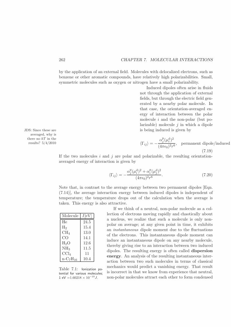
262 CHAPTER 7. MOLECULAR INTERACTIONS
by the application of an external field. Molecules with delocalized electrons, such asbenzene or other aromatic compounds, have relatively high polarizabilities. Small,symmetric molecules such as oxygen or nitrogen have a small polarizability.
Induced dipoles often arise in fluidsnot through the application of externalfields, but through the electric field gen-erated by a nearby polar molecule. Inthat case, the orientation-averaged en-ergy of interaction between the polarmolecule i and the non-polar (but po-larizable) molecule j in which a dipoleis being induced is given byJDS: Since these are
averaged, why isthere no kT in theresults? 5/4/2010 〈Γij〉 = −
αpj (µ
di )
2
(4πǫ0)2r6, permanent dipole/induced
(7.19)If the two molecules i and j are polar and polarizable, the resulting orientation-averaged energy of interaction is given by
〈Γij〉 = −αpj (µ
di )
2 + αpi (µ
dj )
2
(4πǫ0)2r6. (7.20)
Note that, in contrast to the average energy between two permanent dipoles [Eqn.(7.14)], the average interaction energy between induced dipoles is independent oftemperature; the temperature drops out of the calculation when the average istaken. This energy is also attractive.
Molecule I[eV]
He 24.5H2 15.4CH4 13.0CO 14.1H2O 12.6NH3 11.5CCl4 11n-C7H16 10.4
Table 7.1: Ionization po-tential for various molecules;1 eV =1.60218 × 10⁻¹⁹J .
If we think of a neutral, non-polar molecule as a col-lection of electrons moving rapidly and chaotically abouta nucleus, we realize that such a molecule is only non-polar on average; at any given point in time, it exhibitsan instantaneous dipole moment due to the fluctuationsof the electrons. This instantaneous dipole moment caninduce an instantaneous dipole on any nearby molecule,thereby giving rise to an interaction between two induceddipoles. The resulting energy is often called dispersionenergy. An analysis of the resulting instantaneous inter-action between two such molecules in terms of classicalmechanics would predict a vanishing energy. That resultis incorrect in that we know from experience that neutral,non-polar molecules attract each other to form condensed
7.2. INTERMOLECULAR INTERACTIONS 263
phases. It is therefore necessary to invoke quantum me-chanics and analyze the behavior of the electrons using Schrodinger’s equation. Asimple analysis of dispersion energy in terms of quantum mechanics can be foundin the literature. . Here we limit our discussion to the resulting expression for the References? JDS
07/11/2007energy of interaction
Γij = −3
2
αpi α
pj
ǫ20r6
(h2ν0iν0j
hν0i + hν0j
)
, induced dipole/induced dipole, (7.21)
where h is Planck’s constant and ν0 is the electronic frequency of the molecule in Should the Planckconstants in thedenominator reallybe h? JDS07/11/2007
its lowest energy state. It turns out that the product hν0 is well approximated bythe first ionization potential I/4π (the energy required to ionize a molecule fromthe ground state). Eqn. (7.21) can therefore be approximated by
Γij ∼= −3
2
αpi α
pj
(4πǫ0)2r6
(IiIjIi + Ij
)
, induced dipole/induced dipole. (7.22)
Table (7.1) provides values for the first ionization potentials of several molecules;Table (7.2) provides values for the polarizabilities. In general, large molecules aremore polarizable than small ones. The opposite is true for ionization potentials.It is also interesting to note that, in contrast to the polarizabilities, the ionizationpotentials don’t change considerably from molecule to molecule.
For small molecules, a typical value of αp/4πǫ0 is ≈ 1.5 × 10⁻³⁰ m3. A typicalionization potential is I ≈ 2×10⁻¹⁸ J . Two small molecules in contact are separatedby approximately 0.3 nm, making their dispersion energy of interaction (at contact)approximately Γ ≈ −4.6 × 10⁻²¹J , or 1 kBT at room temperature. This simplenumerical calculation should be contrasted with the hand-waving arguments usedearlier [§7.2.1] to explain the significance of kBT .
Dispersion interactions such as those described by Equation (7.22) arise betweenvirtually all molecules, whether they are polar or not, asymmetric or symmetric.They always give rise to a net attraction between two molecules, and they are infact responsible for the occurrence of condensed, liquid or solid phases in simplesubstances which exhibit negligible permanent dipoles or quadrupoles (e.g., noblegases). For example, we can consider the case of Argon, which forms a closely packedsolid at low temperatures. Each Ar atom in the solid lattice is surrounded by 12nearest neighbors, separated by a distance 0.376nm. This corresponds to 6 “bonds”.If interactions between atoms further away are also considered, this number risesto approximately 7.22. The molar cohesive energy density of an Argon crystal can
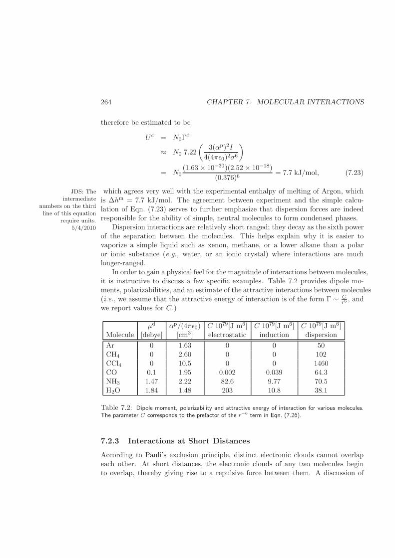
264 CHAPTER 7. MOLECULAR INTERACTIONS
therefore be estimated to be
U c = N0Γc
≈ N0 7.22
(3(αp)2I
4(4πǫ0)2σ6
)
= N0(1.63 × 10⁻³⁰)(2.52 × 10⁻¹⁸)
(0.376)6= 7.7 kJ/mol, (7.23)
which agrees very well with the experimental enthalpy of melting of Argon, whichJDS: Theintermediate
numbers on the thirdline of this equation
require units.5/4/2010
is ∆hm = 7.7 kJ/mol. The agreement between experiment and the simple calcu-lation of Eqn. (7.23) serves to further emphasize that dispersion forces are indeedresponsible for the ability of simple, neutral molecules to form condensed phases.
Dispersion interactions are relatively short ranged; they decay as the sixth powerof the separation between the molecules. This helps explain why it is easier tovaporize a simple liquid such as xenon, methane, or a lower alkane than a polaror ionic substance (e.g., water, or an ionic crystal) where interactions are muchlonger-ranged.
In order to gain a physical feel for the magnitude of interactions between molecules,it is instructive to discuss a few specific examples. Table 7.2 provides dipole mo-ments, polarizabilities, and an estimate of the attractive interactions between molecules(i.e., we assume that the attractive energy of interaction is of the form Γ ∼ C
r6 , andwe report values for C.)
µd αp/(4πǫ0) C 1079[J m6] C 1079[J m6] C 1079[J m6]Molecule [debye] [cm3] electrostatic induction dispersion
Ar 0 1.63 0 0 50CH4 0 2.60 0 0 102CCl4 0 10.5 0 0 1460CO 0.1 1.95 0.002 0.039 64.3NH3 1.47 2.22 82.6 9.77 70.5H2O 1.84 1.48 203 10.8 38.1
Table 7.2: Dipole moment, polarizability and attractive energy of interaction for various molecules.The parameter C corresponds to the prefactor of the r−6 term in Eqn. (7.26).
7.2.3 Interactions at Short Distances
According to Pauli’s exclusion principle, distinct electronic clouds cannot overlapeach other. At short distances, the electronic clouds of any two molecules beginto overlap, thereby giving rise to a repulsive force between them. A discussion of
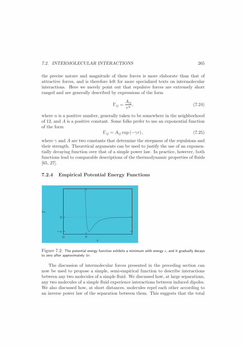
7.2. INTERMOLECULAR INTERACTIONS 265
the precise nature and magnitude of these forces is more elaborate than that ofattractive forces, and is therefore left for more specialized texts on intermolecularinteractions. Here we merely point out that repulsive forces are extremely shortranged and are generally described by expressions of the form
Γij =Aijrn
, (7.24)
where n is a positive number, generally taken to be somewhere in the neighborhoodof 12, and A is a positive constant. Some folks prefer to use an exponential functionof the form
Γij = Aij exp (−γr) , (7.25)
where γ and A are two constants that determine the steepness of the repulsions andtheir strength. Theoretical arguments can be used to justify the use of an exponen-tially decaying function over that of a simple power law. In practice, however, bothfunctions lead to comparable descriptions of the thermodynamic properties of fluids[65, 27].
7.2.4 Empirical Potential Energy Functions
r
Γ
0 σ−ǫ
0
Figure 7.2: The potential energy function exhibits a minimum with energy ǫ, and it gradually decaysto zero after approximately 4σ.
The discussion of intermolecular forces presented in the preceding section cannow be used to propose a simple, semi-empirical function to describe interactionsbetween any two molecules of a simple fluid. We discussed how, at large separations,any two molecules of a simple fluid experience interactions between induced dipoles.We also discussed how, at short distances, molecules repel each other according toan inverse power law of the separation between them. This suggests that the total
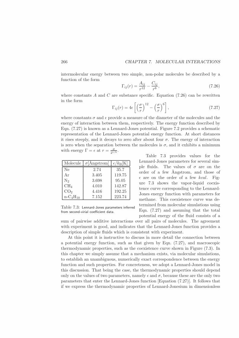
266 CHAPTER 7. MOLECULAR INTERACTIONS
intermolecular energy between two simple, non-polar molecules be described by afunction of the form
Γij(r) =Aijr12
− Cijr6, (7.26)
where constants A and C are substance specific. Equation (7.26) can be rewrittenin the form
Γij(r) = 4ǫ
[(σ
r
)12−(σ
r
)6]
, (7.27)
where constants σ and ǫ provide a measure of the diameter of the molecules and theenergy of interaction between them, respectively. The energy function described byEqn. (7.27) is known as a Lennard-Jones potential. Figure 7.2 provides a schematicrepresentation of the Lennard-Jones potential energy function. At short distancesit rises steeply, and it decays to zero after about four σ. The energy of interactionis zero when the separation between the molecules is σ, and it exhibits a minimumwith energy Γ = ǫ at r = σ
21/6.
Molecule σ[Angstrom] ǫ/kB[K]
Ne 2.74 35.7Ar 3.405 119.75N2 3.698 95.05CH4 4.010 142.87CO2 4.416 192.25n-C4H10 7.152 223.74
Table 7.3: Lennard-Jones parameters inferredfrom second-virial coefficient data.
Table 7.3 provides values for theLennard-Jones parameters for several sim-ple fluids. The values of σ are on theorder of a few Angstrom, and those ofǫ are on the order of a few kcal. Fig-ure 7.3 shows the vapor-liquid coexis-tence curve corresponding to the Lennard-Jones energy function with parameters formethane. This coexistence curve was de-termined from molecular simulations usingEqn. (7.27) and assuming that the totalpotential energy of the fluid consists of a
sum of pairwise additive interactions over all pairs of molecules. The agreementwith experiment is good, and indicates that the Lennard-Jones function provides adescription of simple fluids which is consistent with experiment.
At this point it is instructive to discuss in more detail the connection betweena potential energy function, such as that given by Eqn. (7.27), and macroscopicthermodynamic properties, such as the coexistence curve shown in Figure (7.3). Inthis chapter we simply assume that a mechanism exists, via molecular simulations,to establish an unambiguous, numerically exact correspondence between the energyfunction and such properties. For concreteness, we adopt a Lennard-Jones model inthis discussion. That being the case, the thermodynamic properties should dependonly on the values of two parameters, namely ǫ and σ, because these are the only twoparameters that enter the Lennard-Jones function [Equation (7.27)]. It follows thatif we express the thermodynamic properties of Lennard-Jonesium in dimensionless
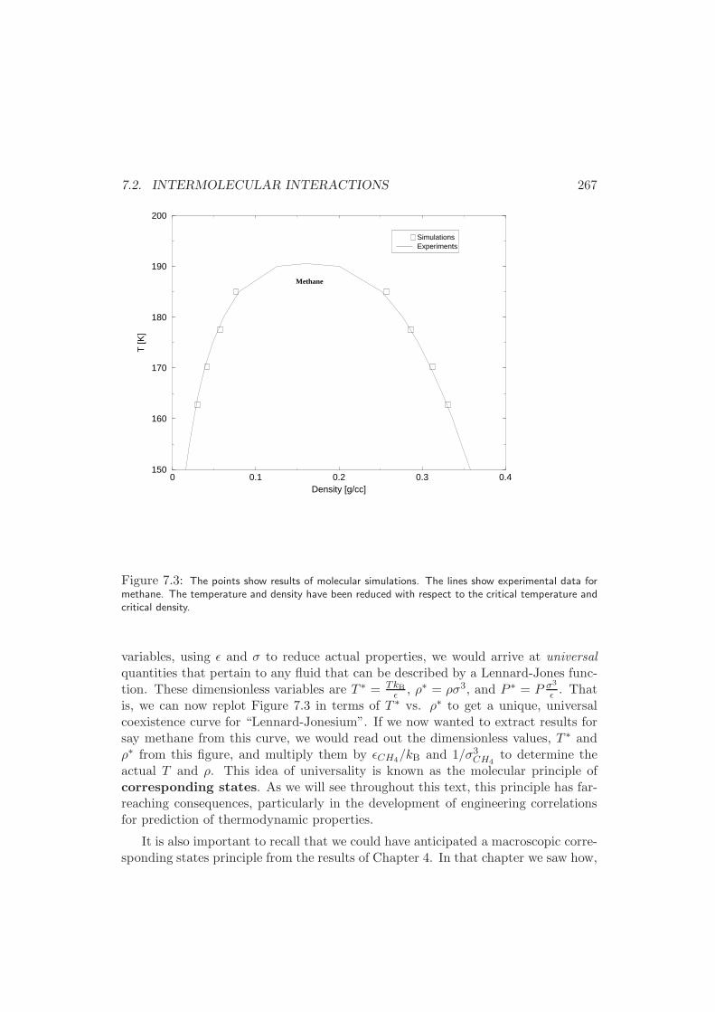
7.2. INTERMOLECULAR INTERACTIONS 267
0 0.1 0.2 0.3 0.4Density [g/cc]
150
160
170
180
190
200
T [K
]
SimulationsExperiments
Methane
Figure 7.3: The points show results of molecular simulations. The lines show experimental data formethane. The temperature and density have been reduced with respect to the critical temperature andcritical density.
variables, using ǫ and σ to reduce actual properties, we would arrive at universalquantities that pertain to any fluid that can be described by a Lennard-Jones func-tion. These dimensionless variables are T ∗ = TkB
ǫ , ρ∗ = ρσ3, and P ∗ = P σ3
ǫ . Thatis, we can now replot Figure 7.3 in terms of T ∗ vs. ρ∗ to get a unique, universalcoexistence curve for “Lennard-Jonesium”. If we now wanted to extract results forsay methane from this curve, we would read out the dimensionless values, T ∗ andρ∗ from this figure, and multiply them by ǫCH4/kB and 1/σ3CH4
to determine theactual T and ρ. This idea of universality is known as the molecular principle ofcorresponding states. As we will see throughout this text, this principle has far-reaching consequences, particularly in the development of engineering correlationsfor prediction of thermodynamic properties.
It is also important to recall that we could have anticipated a macroscopic corre-sponding states principle from the results of Chapter 4. In that chapter we saw how,

268 CHAPTER 7. MOLECULAR INTERACTIONS
applying thermodynamic stability at the critical point of a pure fluid, we can arriveat a universal coexistence curve (for a given model) by reducing thermodynamicquantities by the corresponding values evaluated at the critical point (i.e. Tr =
TTc,
vr =vvc
and Pr =PPc.) In the particular case of fluids described by a van der Waals
equation of state, we showed that a “universal” equation can be written in the form
Pr =8Tr
3vr − 1+
3
vr2.
This connection between molecular and macroscopic corresponding states suggeststhat we should be able to establish a connection between the properties of a purefluid and its Lennard-Jones parameters. That connection can be made throughthe critical point: for Lennard-Jonesium, the critical temperature and density areTc
∗ ∼= 1.32 and ρc∗ ∼= 0.29. If the critical point of an actual fluid of interest is known,
it is possible to obtain Lennard-Jones parameters that will capture the experimentalbehavior in the region near the critical point. For argon, for example, the criticalpoint is at Tc = 150.8 K and ρc = 0.01335 mol/cm3; appropriate Lennard-Jonesparameters are therefore ǫ/kB = 114.2 K and σ = 3.39 A.
Note that more anisotropic molecules, such as long alkanes, can be describedas a collection of several Lennard-Jones interaction sites connected to each other.For the particular case of a long alkane, each interaction site could, for example, beassumed to represent an individual CH2 functional group. Figure 7.4 shows results ofmolecular simulations of a multi-site Lennard-Jones model for alkanes. As that figureillustrates, this simple model describes experimental coexistence curves reasonablywell. When molecules have a dipole moment, or when they have charges (as ions do),the Lennard-Jones function of Eqn. (7.27) must be supplemented by dipole-dipoleinteractions, which are proportional to r−3, and by Coulombic interactions, whichare proportional to r−1. In that case Γ(r) is given by an expression of the form
Γ(r) = 4ǫ
[(σ
r
)12−(σ
r
)6]
+(µd)2
4πǫ0r3+
q2
4πǫ0r, (7.28)
where µd and q denote the dipole moment and the charge of the particles, re-spectively. While most fluids exhibit dipolar and electrostatic interactions, for thepurposes of our discussion here we will assume that Lennard-Jones interactions aresufficient to describe with reasonable accuracy the behavior of simple fluids.
For simplicity, our discussion of the Lennard-Jones energy function has beenrestricted to pure fluids. In the case of mixtures, the interaction energy betweenunlike molecules i and j is given by
Γij(r) = 4ǫij
[(σijr
)12−(σijr
)6]
. (7.29)
7.2. INTERMOLECULAR INTERACTIONS 269
Parameter σij defines the length scale for interactions between molecules i and jand, as discussed earlier, for pure fluids it can be viewed as a measure of the diameterof a molecule. It is therefore logical to assume that diameters are additive and, formixtures, assume an arithmetic mixing rule for σij:
σij =σi + σj
2. (7.30)
For the strength of the interactions, we can go back to our discussion of intermolec-ular forces and recall that, according to Equations (7.22) and (7.26), the coeffi-cient that governs the strength of attractive, dispersive interactions between twomolecules depends on the product of the ionization potentials and polarizabilities ofthe molecules. The ionization potentials do not differ too much from one moleculeto another. For simplicity, we can assume them to be constant and concentrateour attention on the polarizabilities. In that case (see Problem 7.4.C), it can beshown that a geometric mixing rule, i.e.
ǫij = (ǫiǫj)12 , (7.31)
provides a reasonable means of estimating unlike interaction energies from pure-component values of ǫ.
It is important to note that, in general, the expressions given above for Γ(r)do not lead to closed-form expressions for the thermodynamic properties of fluids.It is therefore common to assume simplified interaction-energy functions or modelswhich capture some of the essential physics of molecular interactions, but which aremore tractable from a mathematical point of view. One such model is the hard-sphere fluid, where Γ(r) takes the form of a step function. Another example isprovided by the square-well fluid, in which intermolecular interactions are assumedto be infinitely large below a certain “overlap” distance, negative and constant forintermediate separations, and zero beyond a certain threshold separation.
7.2.5 Hydrogen Bonds
Hydrogen bonds deserve special mention, in that they are 10 to 40 times strongerthan simple dispersion interactions, but considerably weaker than ionic bonds. Hy-drogen bonds are particularly relevant in water; they are responsible for its highboiling point and high enthalpy of vaporization, as well as other anomalies such asthe maximum in density that occurs at 1 bar and 4C. Note, however, that theyalso arise in numerous other substances (e.g., methanol, hydrogen fluoride, etc.).
The intra-molecular distance of an O-H bond in a water molecule is 0.1nm. Theintermolecular distance between nearest-neighbor oxygen and hydrogen atoms inwater is approximately 0.176nm, which is considerably smaller than the distance
270 CHAPTER 7. MOLECULAR INTERACTIONS
that would be expected from simply summing the van der Waals radii of oxygenand hydrogen atoms. While these numbers suggest that hydrogen bonds have acovalent element to them, it is now accepted that their origin is electrostatic.
Hydrogen bonds are highly directional, and arise not only intermolecularly butalso intramolecularly. Much of the structure of large biological molecules such asproteins or DNA is in fact a direct manifestation of intra-molecular hydrogen bond-ing.
One particularly intriguing consequence of hydrogen bonding interactions is theso-called hydrophobic effect. In the case of water, the tendency to form hydrogenbonds between neighboring molecules leads to the formation of a relatively tighttetrahedral network structure. Molecules that are not able to hydrogen bond withwater are excluded from the network, as shown in Figure 7.5.
7.3 Molecular Simulations
Having established how molecules interact with each other, one of the goals of molec-ular thermodynamics is to determine how these interactions manifest themselves inthe thermodynamic behavior of a fluid. To do that, a connection must be madebetween molecular interactions and measurable, macroscopic thermodynamic quan-tities such as the density, pressure, or heat capacity. For two spherical molecules, theinteraction energy between them depends on how far apart they are. For moleculeswith internal degrees of freedom, the interaction energy also depends on their relativeorientation and their internal configuration. These quantities change continuouslyin time as a result of thermal motion. To estimate average, macroscopic thermody-namic quantities, we must therefore have access to millions of distinct configurationsof the system and take an average over the “instantaneous” properties correspond-ing to each of these. These configurations can be easily generated by resorting towhat are commonly called “molecular simulations”.
For simplicity, it is often assumed that the total energy of a fluid can be de-composed into a sum of pairwise additive interactions. With that assumption, theinternal energy U of a fluid can be written in the form
U =1
2
⟨N∑
i
N∑
j
Γij(rij)
⟩
+ cNkBT, (7.32)
where the sum is conducted over all the N molecules in the system, and wherethe angle brackets denote an average over many configurations of the system. Thefirst term of Eqn. (7.32) corresponds to potential energy contributions, which arisefrom the relative position or arrangement of the molecules. The second term corre-sponds to kinetic energy contributions, arising from the velocity or momenta of the
7.3. MOLECULAR SIMULATIONS 271
molecules; these contributions are responsible for the “simple-ideal-gas” part of anythermodynamic property.
To generate the configurations required to evaluate the average in Eqn. (7.32),one possibility would be to reconstruct a few nanoseconds in the life of a fluid, andto store this information in the form of instantaneous “snapshots” of the system.According to Newton’s law of motion, the force acting on a molecule i gives rise tothe dynamics
~Fi = mi~ai, (7.33)
where mi is the mass of the molecule and ~ai is its acceleration. In a many-moleculefluid, the total force acting on molecule i will be given by the sum of the forces ~Fijexerted on it by all the other molecules,
~Fi =
N∑
j 6=i
~Fij, (7.34)
where the force exerted by molecule j on molecule i is given by
~Fij = −dΓij(~rij)d~rij
. (7.35)
Given that we are trying to recreate the trajectory of a collection of moleculesas they move about in a fluid, it is natural to write a Taylor’s series expansion toestimate the coordinates ~ri(t+ δt) of molecule i a short time later t+ δt
~ri(t+ δt) = ~ri(t) + δt
(∂~ri∂t
)
+1
2(δt)2
(∂2~ri∂t2
)
+ ·
= ~ri(t) + δt~vi(t) +1
2(δt)2~ai(t) + ·
= ~ri(t) + δt~vi(t) +1
2mi(δt)2 ~Fi(t) + ·, (7.36)
where ~vi(t) denotes the velocity of molecule i at time t. If the coordinates andvelocities of all molecules are known at time t, it is possible to calculate the forces~Fi(t) at time t; Eqn. (7.36) can then be used to determine ~ri(t + δt) for eachmolecule i of the system of interest. This process can now be repeated at will,thereby generating a trajectory or “movie” for the system; the total duration of thistrajectory will be τ =
∑
ntδt, where nt is the number of “time steps” employed in
the integration of Eqn. (7.36).The integration process outlined above is typically referred to as a molecular
dynamics simulation. It is nowadays typical to use on the order of 1000 molecules fora simulation, and to use a time step of approximately 10−15s. Given the demands

272 CHAPTER 7. MOLECULAR INTERACTIONS
of these calculations, typical trajectories seldom exceed a few nanoseconds (thecomputational time required by these calculations can be on the order of hoursto days.) For most small-molecule fluids, however, a 1 ns simulation is sufficientto generate reliable estimates of their thermodynamic properties. Simulations aretherefore generally used as computer experiments, capable of revealing importantinsights about a fluid, but they are not used for fast, routine engineering calculations.To do that, we must resort to approximate theoretical treatments, some of which aredescribed in the following sections. Equivalently, one can also use what are called“Monte Carlo simulations”. These are described in a later chapter.
7.4 Virial Expansion
The arguments used above (§4.2.1) to arrive at the van der Waals mechanical equa-tion of state (B.15) are not rigorous. Without a firm understanding of the founda-tions of van der Waals’ equation, it would be difficult to extend it to mixtures, forexample.
As alluded to briefly above, it is possible to use molecular simulations to predictthe thermodynamic properties of a fluid from knowledge of the potential energyof interaction between molecules (e.g., Eqn. (7.27)). Such simulations, however,are numerically demanding and are not apt for fast, reasonable estimates of theproperties of fluids.
For real gases, it is possible to formulate essentially exact equations that relatemolecular interactions between pairs of molecules to the macroscopic, thermody-namic properties of the fluid. In this section, we will restrict our attention to realgases at low to moderate pressures.
For an ideal gas the compressibility factor is
Z :=Pv
RT= 1, ideal gas. (7.37)
For a real gas, which is likely to exhibit deviations from ideality, it is reasonable topropose simple, additive corrections to Eqn. (7.37). Based on our intuition, we canexpect these corrections to become increasingly important as the density of the gasis increased. A power series in the density (see §B.2) satisfies these requirements:
Z = 1 +Bρ+ Cρ2 + . . .
= 1 +B
v+C
v2+ . . . . (7.38)
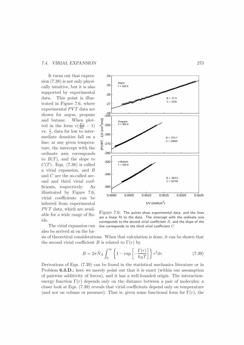
7.4. VIRIAL EXPANSION 273
-28
-27
-26
-25
-24
-280
-270
-260
-250
-240
(PV
/RT
- 1
)V (
cm3 /m
ol)
0.0000 0.0005 0.0010 0.0015 0.0020 0.0025
1/V (mol/cm3)
-360
-340
-320
ArgonT = 250 K
PropaneT = 350 K
n-ButaneT = 400 K
C = 1200B = -27.5
C = 19600
C = 33700
B = -275.7
B = -363.5
Figure 7.6: The points show experimental data, and the linesare a linear fit to the data. The intercept with the ordinate axiscorresponds to the second virial coefficient B, and the slope of theline corresponds to the third virial coefficient C.
It turns out that expres-sion (7.38) is not only physi-cally intuitive, but it is alsosupported by experimentaldata. This point is illus-trated in Figure 7.6, whereexperimental PV T data areshown for argon, propaneand butane. When plot-ted in the form v( PvRT − 1)vs. 1
v , data for low to inter-mediate densities fall on aline; at any given tempera-ture, the intercept with theordinate axis correspondsto B(T ), and the slope toC(T ). Eqn. (7.38) is calleda virial expansion, and Band C are the so-called sec-ond and third virial coef-ficients, respectively. Asillustrated by Figure 7.6,virial coefficients can beinferred from experimentalPV T data, which are avail-able for a wide range of flu-ids.
The virial expansion canalso be arrived at on the ba-sis of theoretical considerations. When that calculation is done, it can be shown thatthe second virial coefficient B is related to Γ(r) by
B = 2πNA
∫ ∞
0
1− exp
[
−Γ(r)
kBT
]
r2dr. (7.39)
Derivations of Eqn. (7.39) can be found in the statistical mechanics literature or inProblem 6.3.D.; here we merely point out that it is exact (within our assumptionof pairwise additivity of forces), and it has a well-founded origin. The interaction-energy function Γ(r) depends only on the distance between a pair of molecules; acloser look at Eqn. (7.39) reveals that virial coefficients depend only on temperature(and not on volume or pressure). That is, given some functional form for Γ(r), the
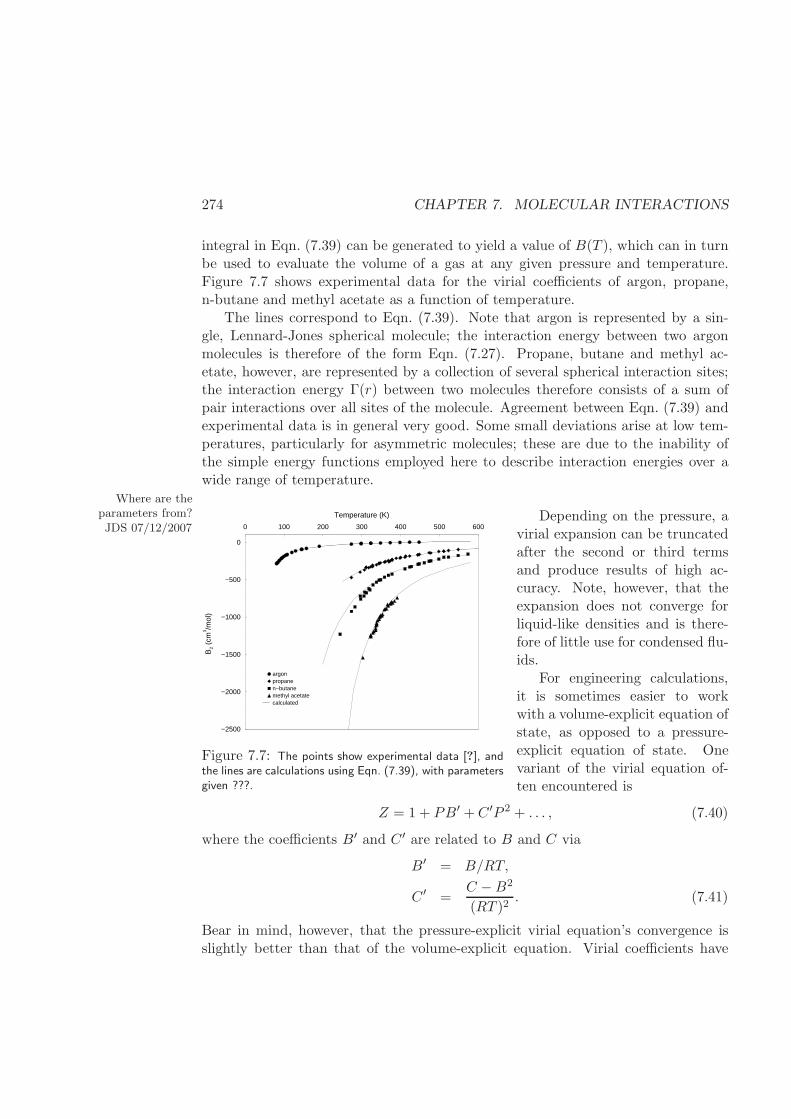
274 CHAPTER 7. MOLECULAR INTERACTIONS
integral in Eqn. (7.39) can be generated to yield a value of B(T ), which can in turnbe used to evaluate the volume of a gas at any given pressure and temperature.Figure 7.7 shows experimental data for the virial coefficients of argon, propane,n-butane and methyl acetate as a function of temperature.
The lines correspond to Eqn. (7.39). Note that argon is represented by a sin-gle, Lennard-Jones spherical molecule; the interaction energy between two argonmolecules is therefore of the form Eqn. (7.27). Propane, butane and methyl ac-etate, however, are represented by a collection of several spherical interaction sites;the interaction energy Γ(r) between two molecules therefore consists of a sum ofpair interactions over all sites of the molecule. Agreement between Eqn. (7.39) andexperimental data is in general very good. Some small deviations arise at low tem-peratures, particularly for asymmetric molecules; these are due to the inability ofthe simple energy functions employed here to describe interaction energies over awide range of temperature.
0 100 200 300 400 500 600
Temperature (K)
−2500
−2000
−1500
−1000
−500
0
B2
(cm
3 /mol
)
argonpropanen−butanemethyl acetatecalculated
Figure 7.7: The points show experimental data [?], andthe lines are calculations using Eqn. (7.39), with parametersgiven ???.
Where are theparameters from?JDS 07/12/2007
Depending on the pressure, avirial expansion can be truncatedafter the second or third termsand produce results of high ac-curacy. Note, however, that theexpansion does not converge forliquid-like densities and is there-fore of little use for condensed flu-ids.
For engineering calculations,it is sometimes easier to workwith a volume-explicit equation ofstate, as opposed to a pressure-explicit equation of state. Onevariant of the virial equation of-ten encountered is
Z = 1 + PB′ +C ′P 2 + . . . , (7.40)
where the coefficients B′ and C ′ are related to B and C via
B′ = B/RT,
C ′ =C −B2
(RT )2. (7.41)
Bear in mind, however, that the pressure-explicit virial equation’s convergence isslightly better than that of the volume-explicit equation. Virial coefficients have
7.4. VIRIAL EXPANSION 275
been measured for a vast number of fluids. A good compilation of experimentaldata can be found in [25].
In the previous section we introduced the molecular principle of correspondingstates, and we made an explicit connection between the experimental critical pointof a pure fluid and that of the Lennard-Jones fluid. That connection allowed us toextract values of σ and ǫ from critical-property data. The idea of correspondingstates can also be discussed in the context of the virial equation. For simplicity, weconsider a virial expansion truncated after the second term. In that case, the PV Tbehavior of a gas can be described completely using Eqn. (7.38). That implies thatthe PV T behavior of the gas is only a function of two parameters, namely ǫ andσ, which enter the equation of state through Expression (7.39). We can thereforerewrite that expression in reduced units according to
B∗(T ∗) =B
2πNAσ3=
∫ ∞
0
1− exp
[
−Γ∗(r∗)T ∗
]
(r∗)2 dr∗. (7.42)
where Γ∗ is used to indicate that the potential energy function can be written asthe product of ǫ times some function of a reduced distance Γ∗ (r∗). In the case ofLennard-Jonesium, we have:
Γ∗ (r∗) = 4
[(1
r∗
)12
−(
1
r∗
)6]
.
The reduced second virial coefficient B∗ can be evaluated as a function of T ∗ byintegrating numerically Eqn. (7.42). This procedure would lead to a universal figureor chart for a given potential-energy function model. For the particular case of theLennard-Jones function, we could read off values of B∗(T ∗) from this chart and relatethese to experimental B(T ) data for a specific fluid, thereby generating estimatesof parameters σ and ǫ.
One important feature of the virial expansion which makes it particularly attrac-tive is that it can be readily extended to mixtures without a need for hand-wavingarguments. For a multicomponent mixture, the virial coefficients of a vapor aregiven by
B =r∑
i=1
r∑
j=1
xixjBij ,
C =
r∑
i=1
r∑
j=1
r∑
k=1
xixjxkCijk, (7.43)
where xi is the mole fraction of component i, Bij denotes the second virial coef-ficient for interactions between molecules of type i and type j, and Cijk denotes
276 CHAPTER 7. MOLECULAR INTERACTIONS
the third virial coefficient for interactions between molecules i, j and k. The ques-tion then arises as to how to estimate Bij for two molecules of different chemicalspecies. Equation (7.39) can be used again to determine B from knowledge of anintermolecular potential-energy function for unlike molecules.
7.5 Equations of State for Liquids
As mentioned above, one of the main shortcomings of the virial equation is that itcannot describe the properties of liquid, or high-density phases. In recent years, newstatistical-mechanical based models have been proposed for such cases. The field ofequation-of-state development has evolved very rapidly in the last decade, and newmodels are published literally every month. The origins of such models, however,are essentially the same and can be summarized in a few lines.
As with the development of the van der Waals’ model, the pressure of a fluid isseparated into repulsive and attractive contributions. It turns out that for liquid-likedensities, the molecular structure of a fluid is dominated by packing arrangements.It is therefore particularly important to determine repulsive contributions to thepressure accurately, as they have a profound effect on the system’s thermodynamicproperties. Developing a quantitative theory for the structure of dense liquids hasbeen one of the main objectives of liquid-state theory over many decades. The ad-vent of molecular simulations has contributed significantly to the refinement of suchtheories. Providing a detailed account of how such models are developed is beyondthe scope of this text. For completeness, however, in this section we describe one ofthe many successful models of this nature, which has the additional feature of beingapplicable to mixtures of simple fluids and mixtures containing long, articulatedpolymer molecules (after minor modifications).
The compressibility factor of a system can be written by an equation of the form
Z =Pv
RT= Z ideal + Zhs + Zdisp, (7.44)
where the superscripts “ideal”, “hs” and “disp” are used to denote ideal, hard-sphere, and dispersion contributions, respectively. Ideal contributions to the pres-sure are given by
Z ideal = 1. (7.45)
Hard-sphere contributions to the compressibility factor are given by an expressionof the form
Zhs =4η − 2η2
(1− η3), (7.46)
where η := πNAρd∗3/6 is the packing fraction of the fluid, and d∗ is the effectiveI added a tilde to NA
to make itAvogadro’s number.Is that correct? JDS
07/12/2007
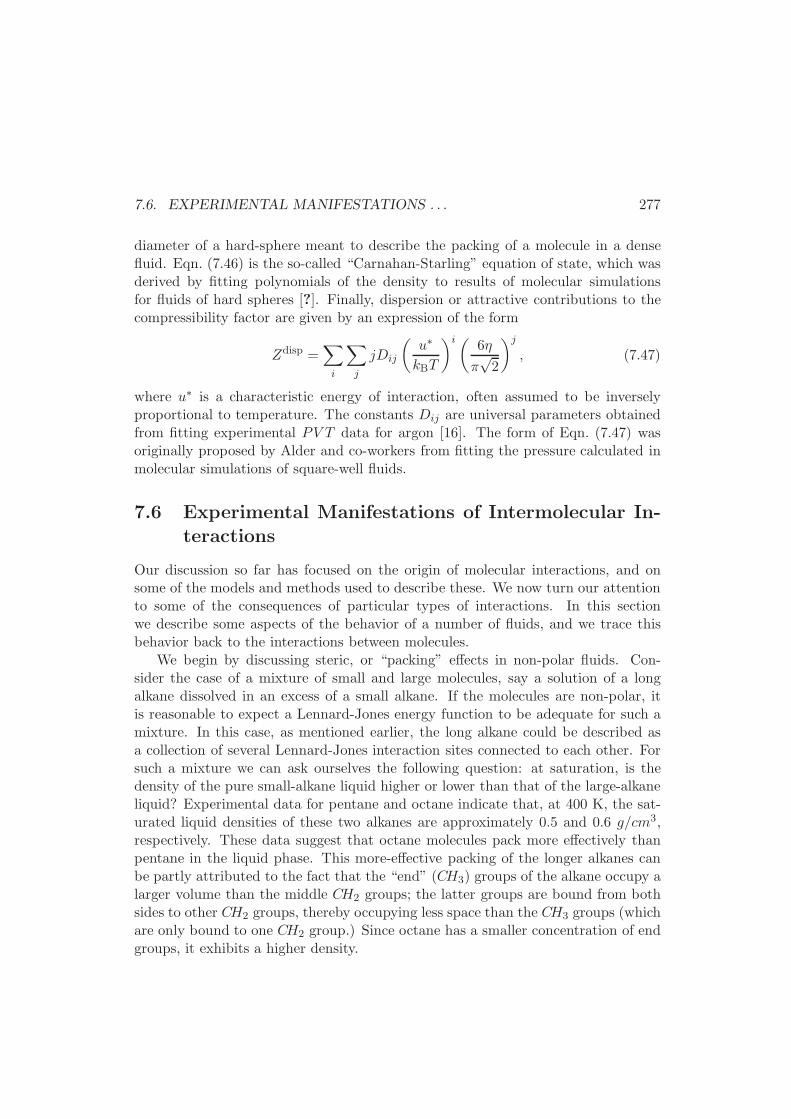
7.6. EXPERIMENTAL MANIFESTATIONS . . . 277
diameter of a hard-sphere meant to describe the packing of a molecule in a densefluid. Eqn. (7.46) is the so-called “Carnahan-Starling” equation of state, which wasderived by fitting polynomials of the density to results of molecular simulationsfor fluids of hard spheres [?]. Finally, dispersion or attractive contributions to thecompressibility factor are given by an expression of the form
Zdisp =∑
i
∑
j
jDij
(u∗
kBT
)i( 6η
π√2
)j
, (7.47)
where u∗ is a characteristic energy of interaction, often assumed to be inverselyproportional to temperature. The constants Dij are universal parameters obtainedfrom fitting experimental PV T data for argon [16]. The form of Eqn. (7.47) wasoriginally proposed by Alder and co-workers from fitting the pressure calculated inmolecular simulations of square-well fluids.
7.6 Experimental Manifestations of Intermolecular In-
teractions
Our discussion so far has focused on the origin of molecular interactions, and onsome of the models and methods used to describe these. We now turn our attentionto some of the consequences of particular types of interactions. In this sectionwe describe some aspects of the behavior of a number of fluids, and we trace thisbehavior back to the interactions between molecules.
We begin by discussing steric, or “packing” effects in non-polar fluids. Con-sider the case of a mixture of small and large molecules, say a solution of a longalkane dissolved in an excess of a small alkane. If the molecules are non-polar, itis reasonable to expect a Lennard-Jones energy function to be adequate for such amixture. In this case, as mentioned earlier, the long alkane could be described asa collection of several Lennard-Jones interaction sites connected to each other. Forsuch a mixture we can ask ourselves the following question: at saturation, is thedensity of the pure small-alkane liquid higher or lower than that of the large-alkaneliquid? Experimental data for pentane and octane indicate that, at 400 K, the sat-urated liquid densities of these two alkanes are approximately 0.5 and 0.6 g/cm3,respectively. These data suggest that octane molecules pack more effectively thanpentane in the liquid phase. This more-effective packing of the longer alkanes canbe partly attributed to the fact that the “end” (CH3) groups of the alkane occupy alarger volume than the middle CH2 groups; the latter groups are bound from bothsides to other CH2 groups, thereby occupying less space than the CH3 groups (whichare only bound to one CH2 group.) Since octane has a smaller concentration of endgroups, it exhibits a higher density.
278 CHAPTER 7. MOLECULAR INTERACTIONS
We can now ask the following question: if we add a small amount of the longalkane to the short alkane, will the density of the mixture be higher or lower thanthat of the pure, small alkane. In this particular case, i.e., for pentane and octane,the answer is relatively straightforward: the density of the resulting mixture can beestimated from a linear combination of the pure-component densities. If, however,the long alkane is relatively long (i.e., if it is a short polyethylene molecule), thelong alkane might not be fully miscible with the short alkane. The solution canphase separate into two distinct liquid phases, or depending on the temperature,pressure, and concentration, the long molecule might drop out of solution and forma semi-crystalline material. The scenario of possibilities for these mixtures is infact relatively complex, and it can all be related to simple interactions such asthose described by the Lennard-Jones function. For mixtures of short and longmolecules, the complex thermodynamic behavior that emerges has most of its originson packing, or steric effects, that come into play when thousands, or millions ofmolecules interact with each other. Such packing effects can in turn be quantifiedthrough the entropy of the mixture, a point to which we come back in our discussionof polymer solutions and blends later in this text.
Isotropic Phase (ρ =0.25, Z = 18.0)
Figure 7.8: Schematic representation of theisotropic phase of a liquid crystal. This configurationof the system was generated by means of molecularsimulations of rod-like molecules. The system is con-fined by two surfaces (shown in red). The distanceZ between the surfaces is equivalent to 18 times thesmaller dimension of the rods.
Another class of systems in whichpacking effects are particularly impor-tant are liquid crystals. Liquid crys-tals are used extensively for a numberof applications (e.g. the screen of lap-top computers); their ability to diffractlight of different wavelengths (and henceexhibit a variety of colors) is relatedto the way in which molecules pack inthe liquid phase. Liquid crystals tendto be elongated, rigid molecules, whoseproperties can be described with reason-able accuracy by assuming they have arod-like or ellipsoidal shape. In the liq-uid state, at sufficiently low densities,molecules pack in a disordered, isotropicmanner. Figure 7.8 shows the instan-taneous structure of an isotropic liquidcrystal, where the aspect ratio of therod-like molecules is 3. As the density(or concentration) is increased, how-
ever, the molecules can adopt an ordered, nematic phase in which molecules adopta well-defined, clear orientation. Figure 7.9 shows the instantaneous structure of
7.6. EXPERIMENTAL MANIFESTATIONS . . . 279
such a nematic phase. This preferred orientation can be turned on or off by con-trolling density, temperature, or the strength of an external field. By manipulatingmolecular orientation, it is possible to control the color of the system and design adisplay.
We now turn our attention to fluids that exhibit hydrogen bonding.Water, of course, is the hydrogen-bonding fluid par excellence, but manyother industrially relevant solvents are also able to hydrogen bond. Inwater, hydrogen bonding arises from the interaction of a lone electronpair on the oxygen atom which undergoes electrostatic interactions withthe electron-deficient hydrogen atoms of other molecules. The strengthof a hydrogen bond is approximately an order of magnitude higher thanthat of simple Lennard-Jones interactions (approximately 15 kBT ). Asa result of these stronger interactions water has a high boiling point(relative to non-polar molecules of the same size); more thermal energyis required to break such hydrogen bonds and vaporize the liquid. Also asa result of hydrogen bonding, water is unable to dissolve other substancesthat do not exhibit such interactions. The solubility of alkanes in water,for example, is remarkably low. The energy required to break enoughhydrogen bonds to form a “cavity” for the alkane is too large to lead toany appreciable solubility. These two
paragraphs that I setoff appear to be justa rewrite of earlierparagraphs in thischapter. This shouldbe shortenedconsiderably andmade as anintroduction to theparagraphs thatfollow. JDS07/12/2007
The consequences of hydrogen bonding are as diverse as they are in-triguing, and are sometimes difficult to anticipate. To illustrate thispoint, we discuss briefly the structural rearrangements undergone bywater molecules around a simple alkane molecule. Our discussion isbased on [14], where a timely discussion of the hydrophobic effect is pre-sented. The presence of an non-polar solute disrupts the hydrogen bondnetwork of water; the magnitude of this effect depends on the shapeand size of the solute molecules. This phenomenon is often referred toas the hydrophobic effect. When the non-polar solute is small, say amethane molecule, the volume that it occupies is less than 5A across;water molecules can adopt hydrogen-bonding patterns that go aroundthat solute without a significant loss of energy. Above a critical size,however, the hydrogen bonding network of water can no longer be main-tained, and some bonds are sacrificed. Near a hydrophobic molecule or ahydrophobic surface, the number of hydrogen-bonding possibilities withthe rest of the fluid is diminished. To minimize that loss, water tends tomove away from the solute, thereby creating an interface around it. Atroom temperature and ambient pressure, that interface is akin to thatwhich forms between a liquid and a vapor. The cost of maintaining this
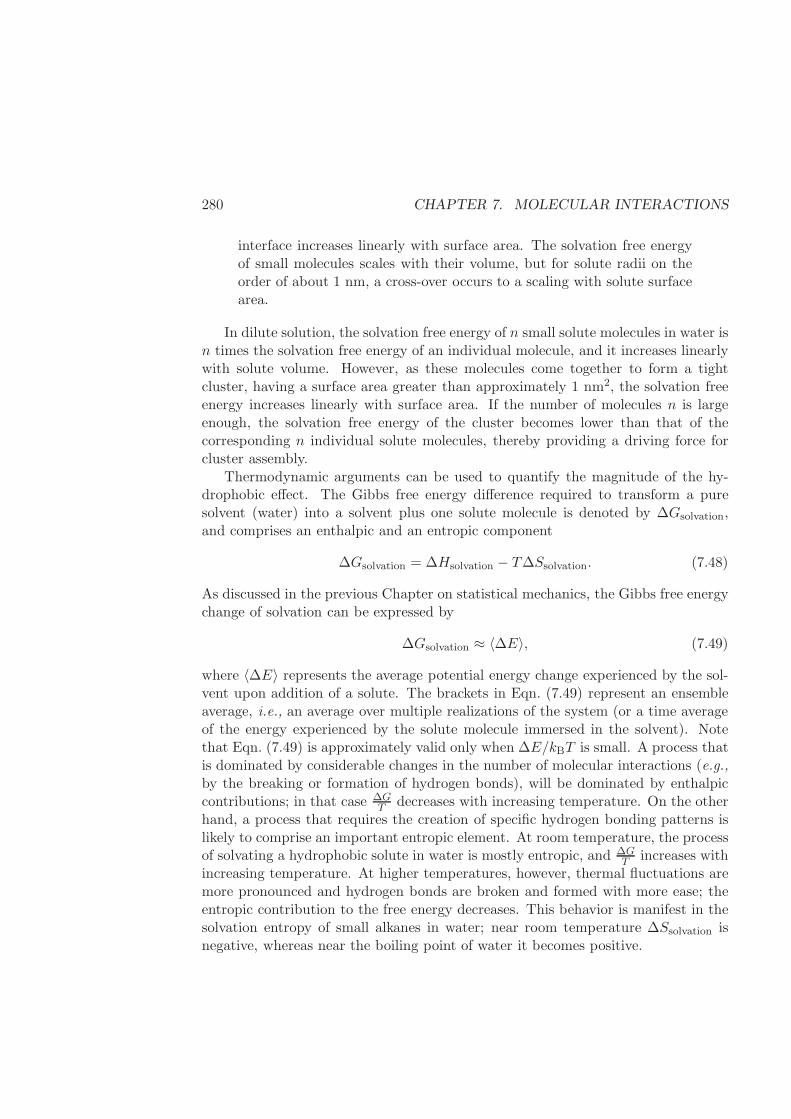
280 CHAPTER 7. MOLECULAR INTERACTIONS
interface increases linearly with surface area. The solvation free energyof small molecules scales with their volume, but for solute radii on theorder of about 1 nm, a cross-over occurs to a scaling with solute surfacearea.
In dilute solution, the solvation free energy of n small solute molecules in water isn times the solvation free energy of an individual molecule, and it increases linearlywith solute volume. However, as these molecules come together to form a tightcluster, having a surface area greater than approximately 1 nm2, the solvation freeenergy increases linearly with surface area. If the number of molecules n is largeenough, the solvation free energy of the cluster becomes lower than that of thecorresponding n individual solute molecules, thereby providing a driving force forcluster assembly.
Thermodynamic arguments can be used to quantify the magnitude of the hy-drophobic effect. The Gibbs free energy difference required to transform a puresolvent (water) into a solvent plus one solute molecule is denoted by ∆Gsolvation,and comprises an enthalpic and an entropic component
∆Gsolvation = ∆Hsolvation − T∆Ssolvation. (7.48)
As discussed in the previous Chapter on statistical mechanics, the Gibbs free energychange of solvation can be expressed by
∆Gsolvation ≈ 〈∆E〉, (7.49)
where 〈∆E〉 represents the average potential energy change experienced by the sol-vent upon addition of a solute. The brackets in Eqn. (7.49) represent an ensembleaverage, i.e., an average over multiple realizations of the system (or a time averageof the energy experienced by the solute molecule immersed in the solvent). Notethat Eqn. (7.49) is approximately valid only when ∆E/kBT is small. A process thatis dominated by considerable changes in the number of molecular interactions (e.g.,by the breaking or formation of hydrogen bonds), will be dominated by enthalpiccontributions; in that case ∆G
T decreases with increasing temperature. On the otherhand, a process that requires the creation of specific hydrogen bonding patterns islikely to comprise an important entropic element. At room temperature, the processof solvating a hydrophobic solute in water is mostly entropic, and ∆G
T increases withincreasing temperature. At higher temperatures, however, thermal fluctuations aremore pronounced and hydrogen bonds are broken and formed with more ease; theentropic contribution to the free energy decreases. This behavior is manifest in thesolvation entropy of small alkanes in water; near room temperature ∆Ssolvation isnegative, whereas near the boiling point of water it becomes positive.
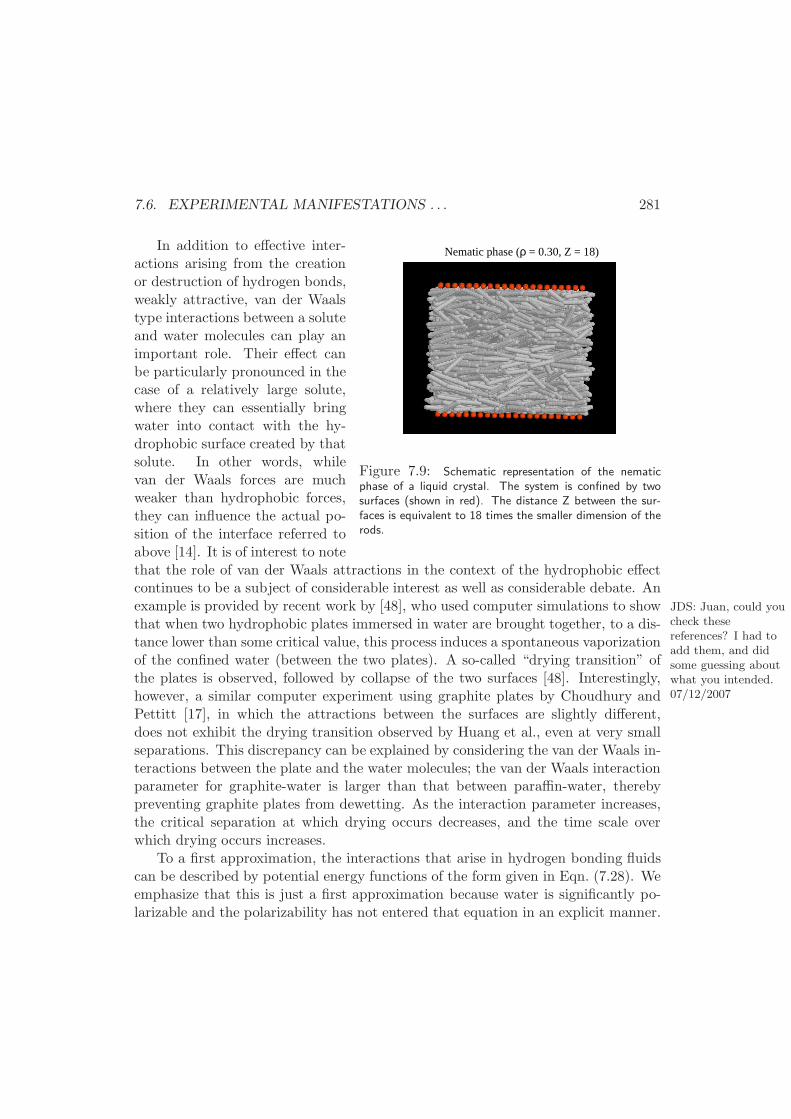
7.6. EXPERIMENTAL MANIFESTATIONS . . . 281
Nematic phase (ρ = 0.30, Z = 18)
Figure 7.9: Schematic representation of the nematicphase of a liquid crystal. The system is confined by twosurfaces (shown in red). The distance Z between the sur-faces is equivalent to 18 times the smaller dimension of therods.
In addition to effective inter-actions arising from the creationor destruction of hydrogen bonds,weakly attractive, van der Waalstype interactions between a soluteand water molecules can play animportant role. Their effect canbe particularly pronounced in thecase of a relatively large solute,where they can essentially bringwater into contact with the hy-drophobic surface created by thatsolute. In other words, whilevan der Waals forces are muchweaker than hydrophobic forces,they can influence the actual po-sition of the interface referred toabove [14]. It is of interest to notethat the role of van der Waals attractions in the context of the hydrophobic effectcontinues to be a subject of considerable interest as well as considerable debate. Anexample is provided by recent work by [48], who used computer simulations to show JDS: Juan, could you
check thesereferences? I had toadd them, and didsome guessing aboutwhat you intended.07/12/2007
that when two hydrophobic plates immersed in water are brought together, to a dis-tance lower than some critical value, this process induces a spontaneous vaporizationof the confined water (between the two plates). A so-called “drying transition” ofthe plates is observed, followed by collapse of the two surfaces [48]. Interestingly,however, a similar computer experiment using graphite plates by Choudhury andPettitt [17], in which the attractions between the surfaces are slightly different,does not exhibit the drying transition observed by Huang et al., even at very smallseparations. This discrepancy can be explained by considering the van der Waals in-teractions between the plate and the water molecules; the van der Waals interactionparameter for graphite-water is larger than that between paraffin-water, therebypreventing graphite plates from dewetting. As the interaction parameter increases,the critical separation at which drying occurs decreases, and the time scale overwhich drying occurs increases.
To a first approximation, the interactions that arise in hydrogen bonding fluidscan be described by potential energy functions of the form given in Eqn. (7.28). Weemphasize that this is just a first approximation because water is significantly po-larizable and the polarizability has not entered that equation in an explicit manner.
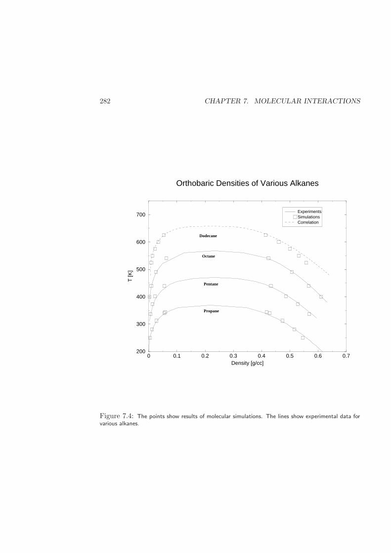
282 CHAPTER 7. MOLECULAR INTERACTIONS
0 0.1 0.2 0.3 0.4 0.5 0.6 0.7Density [g/cc]
200
300
400
500
600
700
T [K
]
Orthobaric Densities of Various Alkanes
ExperimentsSimulationsCorrelation
Propane
Pentane
Octane
Dodecane
Figure 7.4: The points show results of molecular simulations. The lines show experimental data forvarious alkanes.
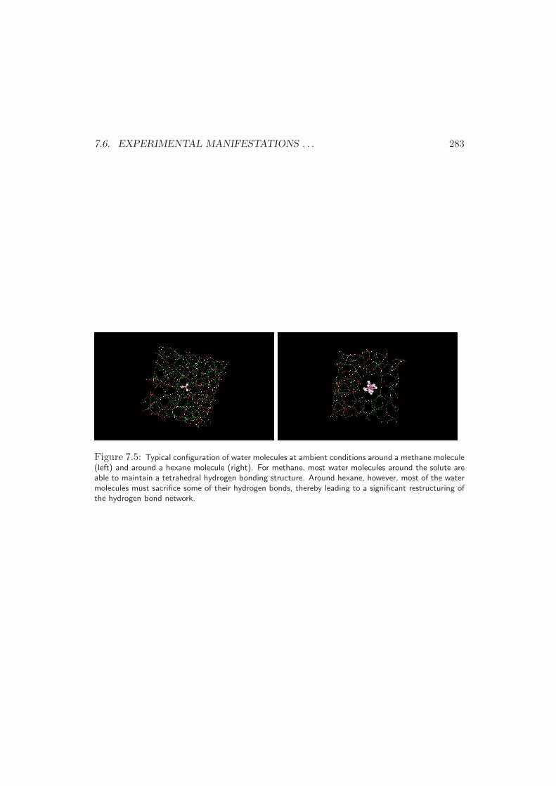
7.6. EXPERIMENTAL MANIFESTATIONS . . . 283
Figure 7.5: Typical configuration of water molecules at ambient conditions around a methane molecule(left) and around a hexane molecule (right). For methane, most water molecules around the solute areable to maintain a tetrahedral hydrogen bonding structure. Around hexane, however, most of the watermolecules must sacrifice some of their hydrogen bonds, thereby leading to a significant restructuring ofthe hydrogen bond network.
284 CHAPTER 7. MOLECULAR INTERACTIONS
7.7 Exercises
7.2.A. Consider the energy of interaction between two, identical polar molecules.The molecules can be represented as rigid rods of length d, with two charges ofopposite sign (q1 and q2) at either end of the rod. The distance between the centersof mass of the two molecules is r. (See Figure 7.1).
a) Show that, provided r ≫ d, the preferred relative orientation between the twomolecules is planar, with the two rods parallel to each other. What is the energy ofinteraction corresponding to that orientation?
b) What is the most unfavorable orientation that the two molecules can have?
7.2.B. Consider a co-linear arrangement in which the shortest distance between twoidentical dipoles is that between the positive charge q1 of one dipole and the negativecharge q′2 of the other dipole. Show that, to leading order, the energy of interactionbetween the dipoles is given by
Γ = −2µd(µd)′
4πǫ0r3, (7.50)
where µd and (µd)′ are the moments of the two dipoles, respectively, and where ris the distance between their centers of mass.Hint: to solve this problem, one can begin by writing an expression for the electro-static potential energy Γ(P ) felt at a point P due to the presence of one dipole. Ifr denotes the distance from P to the center of mass of the dipole, that energy isgiven by
Γ(P ) =1
4πǫ0
(q1r1
+q2r2
)
, (7.51)
where ri is the distance between P and charge qi. By introducing an angle θ betweenthe main axis of the dipole and the line joining point P to the center of mass of thedipole, Eqn. (7.51) can be written as
Γ(P ) =1
4πǫ0
(
q1√
[r2 + z21 + 2z1rcosθ]+
q2√
[r2 + z22 − 2z2rcosθ]
)
, (7.52)
where zi is the distance between the dipole’s center of mass and charge qi. Forr ≫ zi, Eqn. (7.52) can be rewritten in powers of zi/r and expressed in terms ofthe total charge of the dipole q = q1 + q2, the dipole moment µd = q2z2 − q1z1,the quadrupole moment Θ = q1z
21 + q2z
22 , etc. By considering that the center of
mass of a second dipole is located at point P , one can now determine the energy ofinteraction between the two dipoles from
Γ = q′2Γ(q′2) + q′1Γ(q
′1), (7.53)
7.7. EXERCISES 285
where Γ(q′i) represents the electrostatic potential energy experienced at q′i due tothe other (unprimed) dipole.
7.2.C. Use the approach proposed in the previous problem to derive Eqn. (7.13).
7.2.D. Show that the average energy of interaction between two permanent dipolesi and j at a distance r from each other is given by Eqn. (7.14), namely
〈Γij(r)〉 =−2(µdi )
2(µdj )2
(4πǫ0)2kBTr6+ . . . .
Hint: the brackets denote an ensemble average in which distinct configurations ofa system are weighted according to a Boltzmann factor. The average energy ofinteraction between two dipoles is therefore given by
〈Γij(r)〉 =∫ ∫
Γij(~ωi, ~ωj) exp [−Γij(~ωi, ~ωj)] d~ωid~ωj∫ ∫
exp [−Γij(~ωi, ~ωj)] d~ωid~ωj, (7.54)
where ~ωi is used to denote collectively the coordinates of dipole i (i.e., ri, θi, φi),and where d~ωi can be expressed in spherical coordinates as r2i dri sin θidθidφi.
7.2.E. Show that the Lennard-Jones potential energy function exhibits a minimumhaving energy ǫ. At what separation or distance (rmin) between two molecules doesthe minimum occur?
7.2.F. a) Two spherically symmetric molecules having charges qi and qj and sepa-rated by a distance r experience an attractive force between them of magnitude
F =qiqjr2
. (7.55)
When the molecules are separated by a large distance, they do not interact witheach other. Derive an expression for the interaction energy between these moleculesas a function of distance.
b) Two molecules of NH3 exhibit an interaction energy of approximately −20kJ/mol at room temperature. The dipole moment of NH3 is 1.47 Debye, and thepolarizability is approximately 22.6 × 10⁻²⁵ cm3. The ionization potential of NH3
is I = 11.5 eV (1 eV= 1.6×10⁻¹⁹J). The following correlation has been proposed todescribe the potential energy of interaction between two NH3 molecules as a functionof temperature
U =A
T− 13.9kJ. (7.56)
Using your knowledge of intermolecular interactions, please provide a justificationfor the form of this empirical expression. What does constant A represent?
286 CHAPTER 7. MOLECULAR INTERACTIONS
7.2.G. Liquid-crystalline systems are often described in terms of the so-called “Gay-Berne” intermolecular energy function [36]. This function describes the energy ofinteraction between anisotropic, ellipsoidal particles. It is given by an expressionsimilar to Eqn. (7.27), in which the parameters σ and ǫ depend on the relativeorientation of the two molecules. If the axial vectors of the molecules are denotedby ~ui and ~uj, and if ~r is a vector between the centers of mass of two molecules, anorientation-dependent size parameter is defined according to
σGB(~ui, ~uj , ~r) = σ0
(
1− 1
2χ
[(~ui · ~r + ~uj · ~r)21 + χ(~ui · ~uj)
+(~ui · ~r − ~uj · ~r)21− χ(~ui · ~uj)
])− 12
, (7.57)
Parameter χ characterizes the size anisotropy of the molecule, and is given by
χ =κ2 − 1
κ2 + 1. (7.58)
Parameter σ0 is the side-by-side contact distance of a pair of rods, and parameterκ is the aspect ratio (ratio of width to length) of the particles.
The angular dependence of the well-depth of the energy is given by
ǫGB = (ǫ′)(ǫ′′)2, (7.59)
where
ǫ′(~ui, ~uj , ~r) = ǫ0[1− χ2(~ui · ~uj)2
]− 12 ,
ǫ′′(~ui, ~uj , ~r) = ǫ0
(
1− 1
2χ′[(~ui · ~r + ~uj · ~r)21 + χ′(~ui · ~uj)
+(~ui · ~r − ~uj · ~r)21− χ′(~ui · ~uj)
])
,(7.60)
and where
χ′ =
√κ′ − 1√κ′ + 1
. (7.61)
In this equation, κ′ defines the energetic anisotropy of the particles; i.e. how muchstronger the energy of interaction is when the molecules are parallel than whenthey are oriented head-to-tail or head-to-head. With the expressions above, the“Gay-Berne” energy of interaction is given by
ΓGB(~ui, ~uj , ~r) = 4ǫGB
[(σ0dGB
)12
−(σ0dGB
)6]
, (7.62)
with
dGB = r − σGB + σ0. (7.63)
7.7. EXERCISES 287
Plot the energy of interaction between two liquid crystalline molecules of aspectratio 3 in the “head-to-tail” or perpendicular orientation, and in the “parallel” ori-entation. Show that as the aspect ratio of the molecules goes to unity, you recoverthe Lennard-Jones potential. Please discuss the behavior of the intermolecular en-ergy for very long molecules (polymers), in the limit of infinite aspect ratio. Basedon this energy function, also comment on the energy of interaction between two,disk-shaped particles.
7.2.H. Consider a Lennard-Jones potential energy function for the interaction be-tween two, spherically symmetric molecules.
a) Consider a pair of molecules in the gas phase, at some temperature T . Is theaverage distance between the two molecules the same as rmin?
b) Consider a liquid of spherical molecules interacting via a Lennard-Jones en-ergy function Γ(r). For simplicity, assume that the internal energy of the system isgiven by an expression of the form
U =1
2
⟨N∑
i
N∑
j
Γij(rij)
⟩
+ cNkBT, (7.64)
where kB is Boltzmann’s constant, where subscripts i and j are used to denoteindividual molecules, and where N is the number of molecules in the system. Pleasestate clearly the assumptions that went into Eqn. (7.64). Why are there two terms?Why is there a 1
2 factor in the first term? What is the meaning of the angularbrackets? What is the origin of the second term? At liquid-like densities, what isthe average separation between a pair of nearest-neighbor molecules? Is it rmin?
7.2.I. Consider the energy of interaction between two, non-polar molecules. The twomolecules are spherical, but they are of a different chemical nature.
a) Show that if Γii is used to denote the attractive energy of interaction betweentwo molecules of the same species (i), it can be written in the form
Γii = k′αpi2
r6, (7.65)
where αpi is the polarizability of molecule i. Please clarify the physical significance
of constant k′.b) Show that the energy of interaction between molecules of different species can
be approximated by an expression of the form
Γij ≈√
ΓiiΓjj. (7.66)
Please state your assumptions clearly and concisely.
288 CHAPTER 7. MOLECULAR INTERACTIONS
7.2.J. Would you expect chain-like molecules to exhibit corresponding-states behav-ior? Please explain your answer.
7.4.A. a) Use the Lennard-Jones potential energy function to calculate the secondvirial coefficient of “Lennard-Jonesium” and construct a plot of this virial coef-ficient as a function of temperature. To facilitate your analysis, please use re-duced (dimensionless) units for the temperature and the distance (i.e. T ∗ = TkB/ǫ,B∗ = B/(2πNAσ
3), and r∗ = r/σ).b) Find experimental data for the virial coefficients of several simple fluids that
you might expect to be described accurately by a simple Lennard-Jones energyfunction (e.g., noble gases, methane, carbon tetrachloride). Use these data to infer“experimental” values for constants σ and ǫ for those fluids. How well does theLennard-Jones function describe experiments? Do your parameters follow reason-able trends?
c) For the fluids considered in Question b), derive values for the Lennard-Jonesparameters based on critical property data. Compare these parameters to thoseobtained in b) using second-virial coefficient data. Are the parameters identical? ifnot, why are they different?
7.4.B. The energy of interaction between two Lennard-Jones particles of differentspecies i and j can be estimated by using the so-called Lorentz-Berthelot combiningrules, in which the ǫij and σij cross-interaction parameters are given by
ǫij = (ǫiǫj)12 , (7.67)
σij =σi + σj
2. (7.68)
a) Based on the calculations of Exercise (7.4.A., part a), propose a simple andaccurate correlation for B∗(T ∗). Express this correlation in terms of σ and ǫ fora pure fluid. Assuming Lorentz-Berthelot combining rules, write a correlation forthe cross-interaction second virial coefficient in a binary mixture, in terms of pure-component Lennard-Jones parameters.
b) The following correlation has been proposed in the literature [?] to estimatethe second virial coefficients of simple, non-polar fluids consisting of quasi-sphericalmolecules (e.g. methane)
B
vc= 0.430 − 0.886
(T
Tc
)−1
− 0.694
(T
Tc
)−2
. (7.69)
Assuming that the interactions between such molecules can be described by aLennard-Jones potential energy function, rewrite Eqn. (7.69) in terms of the Lennard-Jones parameters σ and ǫ. Does the resulting equation describe the expressionderived in Exercise (7.4.A., part a) with reasonable accuracy?
7.7. EXERCISES 289
c) If you now wanted to develop a correlation for cross-interaction second virialcoefficients in terms of pure-component critical-property data, what mixing ruleswould you propose for the relevant “mixture” pseudo-critical properties?
7.4.C. In the previous exercise, a geometric-mean combining rule was proposed toevaluate the energy parameter for a binary mixture of Lennard-Jones particles.Based on your knowledge of intermolecular interactions, provide a theoretical justi-fication for this combining rule.
7.4.D. The so-called Lennard-Jones (LJ) potential energy function is given by
Γii = 4εi
[(σir
)12−(σir
)6]
, (7.70)
where σ and ǫ are substance-specific parameters.
a) Based on your knowledge of intermolecular interactions, give a theoreticaljustification for the geometric mixing rule that is commonly used to evaluate εij .
b) For the LJ potential, the second virial coefficient B∗ can be evaluated as afunction of temperature T ∗ using the following correlation
B∗ = 0.2336 − 0.68
(1
T ∗
)
− 0.406
(1
T ∗
)2
, (7.71)
where the asterisk denotes a quantity reduced with respect to the Lennard-Jonesparameters, namely σ and ǫ. For linear alkanes, the following correlation is oftenused in practice [?]
B
vc= 0.430 − 0.886
(T
Tc
)−1
− 0.694
(T
Tc
)−2
− 0.0375(n − 1)
(T
Tc
)−4.5
, (7.72)
where n is the number of carbon atoms in the alkane. Using critical property datafor methane and pentane, compare the predictions for B from equations (7.71) and(7.72) at T ∗ = 1 and at T ∗ = 2.5. For which of these two molecules are the twocorrelations in better agreement? Why ?
c) The second virial coefficient is related to the potential energy of interactionbetween two molecules through
B = 2πNA
∫ ∞
0
(
1− exp
[−Γ(r)
kBT
])
r2dr. (7.73)
In order to examine the effects of molecular volume on the properties of a gas, youare asked to propose a simple, tractable model in which only repulsive interactions
290 CHAPTER 7. MOLECULAR INTERACTIONS
are present. One possibility is to use a “hard-sphere” model, in which the interactionenergy between two molecules is of the form
Γ(r) = 0, r ≥ d (7.74)
Γ(r) = ∞, r < d,
where d is the diameter of the molecules. Please sketch the qualitative shape ofΓ(r). Derive an expression for the second virial coefficient of a gas of hard spheres.Does it depend on temperature? Why?
7.4.E. If we assume that the potential energy of interaction of three molecules isgiven by the sum of three, pairwise additive terms (corresponding to the threedistinct pairs that arise in a group of three molecules), the third virial coefficientcan be related to the intermolecular potential energy function by
C = −8π2NA2
3
∫ ∞
0
∫ ∞
0
∫ ~r12+~r13
|~r12−~r13|f12f13f23r12r13r23dr12dr13dr23, (7.75)
where fij = exp(−Γ(rij)/kBT )− 1. Calculate a reduced third virial coefficient andplot it as a function of reduced temperature T ∗. Develop your own, personalized cor-relation for C∗(T ∗) by fitting the results of your calculations to a simple polynomialexpression.
7.4.F. The discussion of second virial coefficients in the text was centered aroundsimple fluids of non-polar, spherical molecules. For engineering work, however,it is important to develop correlations to predict the second virial coefficients ofnon-spherical molecules. Several approaches are available. For linear alkanes, forexample, it has been proposed [?] to estimate second virial coefficients from
B
vc= 0.430 − 0.886
(T
Tc
)−1
− 0.694
(T
Tc
)−2
− 0.0375(n − 1)
(T
Tc
)−4.5
, (7.76)
where n is the number of carbon atoms in the alkane. Another, frequently usedapproach is to resort to the use of an “acentric factor”, usually denoted by ω, whichprovides a measure of the deviations of the potential energy function from sphericalsymmetry. A simple, empirical way of defining ω, due to Pitzer, is given by
ω = − log10
(P sat
Pc
)
T/Tc=0.7
− 1, (7.77)
where P sat is the saturation pressure evaluated at T = 0.7Tc. With this definition,the following correlations can be used to estimate second virial coefficients [?]
BPcRTc
= B(0)
(T
Tc
)
+ ωB(1)
(T
Tc
)
, (7.78)
7.7. EXERCISES 291
where
B(0)
(T
Tc
)
= 0.1445 − 0.330
Tr− 0.1385
T 2r
− 0.0121
T 3r
− 0.000607
T 8r
(7.79)
B(1)
(T
Tc
)
= 0.0637 +0.331
T 2r
− 0.423
T 3r
− 0.008
T 8r
, (7.80)
where Tr = T/Tc.a) Estimate the acentric factors for methane, propane, pentane, octane, and
methanol.b) Compare the predictions of Eqs.(7.76) and (7.78) for methane, propane, pen-
tane and octane. Are their predictions comparable? Which of these two correlationsis more accurate (compare your results to experimental data for alkanes)?
7.4.G. Eqn. (7.78) provides a good representation of the second virial coefficients ofnon-polar or slightly polar fluids. In order to extend its applicability to polar fluids,it has been proposed [?] to add a third term to that equation of the form
B(2)
(T
Tc
)
=c1T 6r
− c2T 8r
. (7.81)
For fluids that do not hydrogen bond, parameter c2 can be assumed to be zero.Parameters c1 and c2 cannot be generalized for wide classes of fluids. For specificchemical families, however, it is possible to arrive at reasonable correlations thatprovide c1 and c2 as a function of the dipole moment. For ethers, for example, it isfound that
log(−c1) = −12.63147 + 2.09681 log µdr , (7.82)
where the reduced dipole moment is defined by
µdr = 0.9869105(µd)2Pc
T 2c
. (7.83)
a) Propose a correlation for c1 as a function of µdr for ketones.b) What parameters c1 and c2 should be used for water?
7.4.H. Consider the van der Waals equation of state, given by
P =RT
v − b− a
v2.
a) Show that parameters a and b of van der Waals equation are related to thecritical constants by
a =27R2T 2
c
64Pc(7.84)
b =RTc8Pc
=vc3. (7.85)
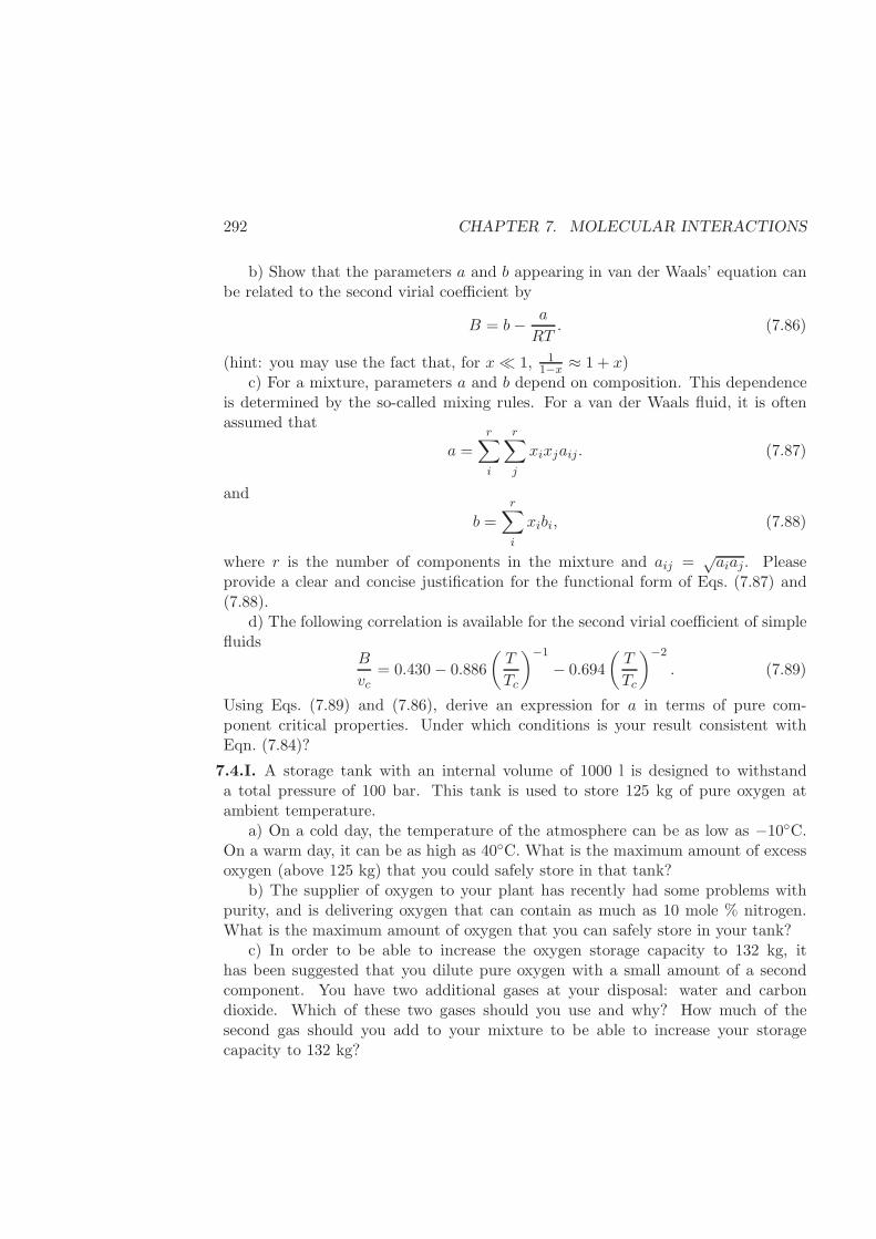
292 CHAPTER 7. MOLECULAR INTERACTIONS
b) Show that the parameters a and b appearing in van der Waals’ equation canbe related to the second virial coefficient by
B = b− a
RT. (7.86)
(hint: you may use the fact that, for x≪ 1, 11−x ≈ 1 + x)
c) For a mixture, parameters a and b depend on composition. This dependenceis determined by the so-called mixing rules. For a van der Waals fluid, it is oftenassumed that
a =r∑
i
r∑
j
xixjaij. (7.87)
and
b =
r∑
i
xibi, (7.88)
where r is the number of components in the mixture and aij =√aiaj. Please
provide a clear and concise justification for the functional form of Eqs. (7.87) and(7.88).
d) The following correlation is available for the second virial coefficient of simplefluids
B
vc= 0.430 − 0.886
(T
Tc
)−1
− 0.694
(T
Tc
)−2
. (7.89)
Using Eqs. (7.89) and (7.86), derive an expression for a in terms of pure com-ponent critical properties. Under which conditions is your result consistent withEqn. (7.84)?
7.4.I. A storage tank with an internal volume of 1000 l is designed to withstanda total pressure of 100 bar. This tank is used to store 125 kg of pure oxygen atambient temperature.
a) On a cold day, the temperature of the atmosphere can be as low as −10C.On a warm day, it can be as high as 40C. What is the maximum amount of excessoxygen (above 125 kg) that you could safely store in that tank?
b) The supplier of oxygen to your plant has recently had some problems withpurity, and is delivering oxygen that can contain as much as 10 mole % nitrogen.What is the maximum amount of oxygen that you can safely store in your tank?
c) In order to be able to increase the oxygen storage capacity to 132 kg, ithas been suggested that you dilute pure oxygen with a small amount of a secondcomponent. You have two additional gases at your disposal: water and carbondioxide. Which of these two gases should you use and why? How much of thesecond gas should you add to your mixture to be able to increase your storagecapacity to 132 kg?
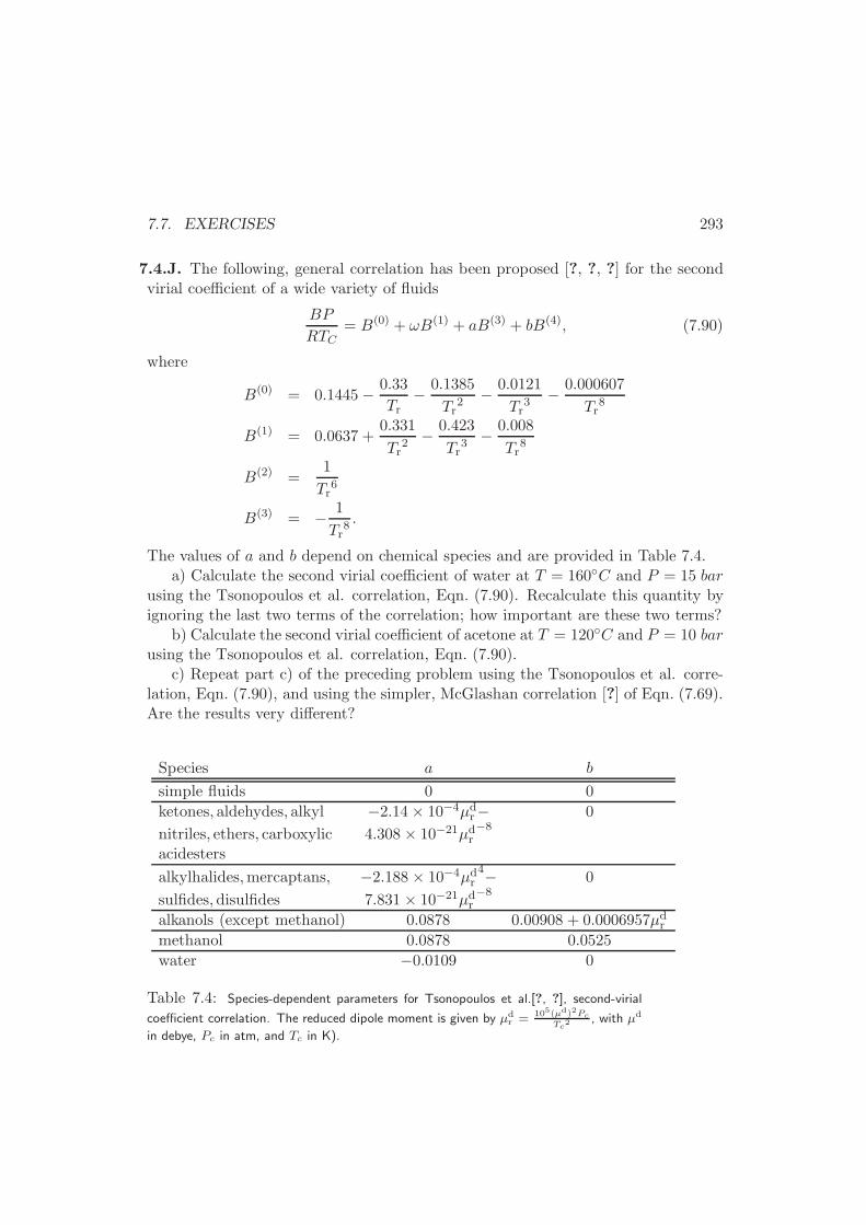
7.7. EXERCISES 293
7.4.J. The following, general correlation has been proposed [?, ?, ?] for the secondvirial coefficient of a wide variety of fluids
BP
RTC= B(0) + ωB(1) + aB(3) + bB(4), (7.90)
where
B(0) = 0.1445 − 0.33
Tr− 0.1385
Tr2 − 0.0121
Tr3 − 0.000607
Tr8
B(1) = 0.0637 +0.331
Tr2 − 0.423
Tr3 − 0.008
Tr8
B(2) =1
Tr6
B(3) = − 1
Tr8 .
The values of a and b depend on chemical species and are provided in Table 7.4.a) Calculate the second virial coefficient of water at T = 160C and P = 15 bar
using the Tsonopoulos et al. correlation, Eqn. (7.90). Recalculate this quantity byignoring the last two terms of the correlation; how important are these two terms?
b) Calculate the second virial coefficient of acetone at T = 120C and P = 10 barusing the Tsonopoulos et al. correlation, Eqn. (7.90).
c) Repeat part c) of the preceding problem using the Tsonopoulos et al. corre-lation, Eqn. (7.90), and using the simpler, McGlashan correlation [?] of Eqn. (7.69).Are the results very different?
Species a b
simple fluids 0 0
ketones, aldehydes, alkyl −2.14× 10⁻⁴µdr− 0
nitriles, ethers, carboxylic 4.308 × 10⁻²¹µdr−8
acidesters
alkylhalides,mercaptans, −2.188 × 10⁻⁴µdr4− 0
sulfides,disulfides 7.831 × 10⁻²¹µdr−8
alkanols (except methanol) 0.0878 0.00908 + 0.0006957µdrmethanol 0.0878 0.0525
water −0.0109 0
Table 7.4: Species-dependent parameters for Tsonopoulos et al.[?, ?], second-virial
coefficient correlation. The reduced dipole moment is given by µdr = 105(µd)2Pc
Tc2, with µd
in debye, Pc in atm, and Tc in K).

294 CHAPTER 7. MOLECULAR INTERACTIONS
Chapter 8
Fugacity and Vapor-LiquidEquilibrium
Hell is other people’s notation.
– with apologies to Jean-Paul Sartre.
In Chapter 4 we saw how simple stability criteria derived from the postulateshave important consequences for calculation of vapor-liquid equilibria. More specif-ically, we discussed how the spinodal curve of a pure fluid defines the boundarybetween locally stable and unstable states, and we also saw how global stabilityleads to guidelines for calculation of binodal, or coexistence curves.
As the number of components of a mixture increases, stability criteria becomeincreasingly complex and are more difficult to apply, although the principles arethe same. Calculations of phase equilibria for multicomponent mixtures thereforebecome more elaborate. These calculations are commonplace in applications, and itis therefore important to have an efficient machinery to address this problem. Thischapter presents that machinery.
Previous chapters dealt mostly with pure component systems. For these wefirst introduced the idea of fundamental relations for U or for S (Chapter 2), andthen, through Legendre transforms, we introduced fundamental relations in thegeneralized potentials (Chapter 3). In Chapter 4 we showed how these fundamentalrelations for a one-component system can be derived from two equations of state,typically a mechanical equation of state, and a thermal equation of state. We alsoshowed in Chapter 6 how to derive fundamental relations from simple molecularmodels.
However, in Chapter 4 we also showed how many things could be accomplishedthrough the mechanical equation of state alone, such as vapor-liquid equilibrium
295
296 CHAPTER 8. FUGACITY AND VAPOR-LIQUID EQUILIBRIUM
and residual properties. For multicomponent vapor-liquid equilibrium, we will findin this chapter that mechanical equations of state are sufficient when we use aquantity called fugacity in place of the chemical potential. The fugacity has theadded advantage of being easier to work with at low pressures than is the chemicalpotential. Therefore, in reference books, technical articles and engineering reports,one rarely sees a fundamental relation for multicomponent mixtures.
We begin by recalling the equations for phase equilibria in bulk multicomponentsystems. As a specific example, we also revisit a mixture of ideal gases. Beforeintroducing fugacities, we define partial molar properties—an important conceptin mixtures. This definition, when combined with residual properties, provides asimple definition for fugacities. Unfortunately, the notation in the literature is verycumbersome, and it is necessary to introduce it all here. We recommend that thereader works hard in this chapter to memorize the definitions already mentioned andthe ones that follow: partial molar properties, fugacity, fugacity coefficient, excessproperties, activity, activity coefficient, the Lewis Mixing Rule (Ideal Mixing) andthe Poynting Correction Factor. These definitions are the just the preliminary—necessary!—tools.
8.1 General Equations of Phase Equilibria
Engineering problems often require calculation of the distribution of several compo-nents through the various phases that constitute a system. Consider, for example,the separation of alcohol and water by distillation. In order to determine how longa water-alcohol mixture must be boiled to achieve a certain degree of separation, itis necessary to know the composition of the vapor and liquid phases in equilibriumwith each other at any given temperature and pressure. For the more general caseof separation of a multicomponent mixture into its individual constituents (e.g., theseparation of crude oil into asphaltenes, gasoline, jet fuel, and light gases), it is im-portant to calculate the concentration of each component throughout a multiphasesystem as a function of temperature and pressure.
In this section, we summarize general results found earlier in the book that areparticularly important for phase equilibrium calculations and derivations. Theserelations are valid for all species, all fundamental relations, all equations of state,all mixing models, etc.
Recall in §§2.7 and 2.8 we showed that two subsystems that can exchange energy,volume, and mass must have equal temperature, pressure and chemical potential.If we have two phases in equilibrium, e.g., two immiscible liquids, or a liquid phaseand gas phase, they exchange heat, mass and volume, so we can write
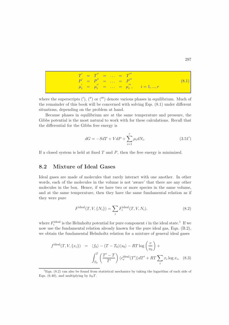
297
T′
= T′′
= . . . = T′′′
P′
= P′′
= . . . = P′′′
µ′i = µ
′′i = . . . = µ
′′′i , i = 1, ..., r
(8.1)
where the superscripts (′), (′′) or (′′′) denote various phases in equilibrium. Much ofthe remainder of this book will be concerned with solving Eqs. (8.1) under differentsituations, depending on the problem at hand.
Because phases in equilibrium are at the same temperature and pressure, theGibbs potential is the most natural to work with for these calculations. Recall thatthe differential for the Gibbs free energy is
dG = −SdT + V dP +r∑
i=1
µidNi. (3.51′)
If a closed system is held at fixed T and P , then the free energy is minimized.
8.2 Mixture of Ideal Gases
Ideal gases are made of molecules that rarely interact with one another. In otherwords, each of the molecules in the volume is not ‘aware’ that there are any othermolecules in the box. Hence, if we have two or more species in the same volume,and at the same temperature, then they have the same fundamental relation as ifthey were pure
F ideal(T, V, Ni) =∑
i
F ideali (T, V,Ni). (8.2)
where F ideali is the Helmholtz potential for pure component i in the ideal state.1 If we
now use the fundamental relation already known for the pure ideal gas, Eqn. (B.2),we obtain the fundamental Helmholtz relation for a mixture of general ideal gases
f ideal(T, V, xi) = 〈f0〉 − (T − T0)〈s0〉 −RT log
(v
v0
)
+
∫ T
T0
(T ′ − T
T ′
)
〈cidealv (T ′)〉dT ′ +RT∑
i
xi log xi, (8.3)
1Eqn. (8.2) can also be found from statistical mechanics by taking the logarithm of each side ofEqn. (6.40), and multiplying by kBT .
298 CHAPTER 8. FUGACITY AND VAPOR-LIQUID EQUILIBRIUM
where the angular brackets here indicate a molar average: 〈m〉 := ∑
i ximi, mi ≡so,i, fo,i, c
idealv,i . Remember that the subscript zero refers to the thermodynamic
properties at the reference temperature T0 and specific volume v0.
Since this is a fundamental relation, we can find all equations of state. Ofparticular interest is to see how thermodynamic properties at fixed T and P changeupon mixing. Using the usual manipulations to obtain equations of state, we findfrom Eqn. (8.3)
uideal(T, P, xi) =∑
i
xiupure, ideali (T, P )
videal(T, P, xi) =∑
i
xivpure, ideali (T, P )
hideal(T, P, xi) =∑
i
xihpure, ideali (T, P )
sideal(T, P, xi) =∑
i
xispure, ideali (T, P )−R
∑
i
xi log xi
f ideal(T, P, xi) =∑
i
xifpure, ideali (T, P ) +RT
∑
i
xi log xi
gideal(T, P, xi) =∑
i
xigpure, ideali (T, P ) +RT
∑
i
xi log xi
µidealj (T, P, xi) = µpure, idealj (T, P ) +RT log xj . (8.4)
The first three results are expected, since the molecules do not interact energetically.Physically, these results mean that if we mix two different ideal gases at the sametemperature and pressure, the volume will not change; hence, there is no workexchanged with the environment. Also, the internal energy does not change, sothere is no heat exchanged with the environment.
The result for entropy is interesting because of the sign of the mixing term. Sinceall mole fractions are less than unity, and the logarithm of a fraction is negative,the entropy of mixing is positive; ideal gases mix spontaneously. The results for thefree energies follow because of their definitions using entropy. These results are alsothe basis for the “Lewis Mixing” approximation that we encounter below.
8.3 Mixtures: Partial Molar Properties
8.3.1 Definition of a Partial Molar Property
To introduce the concept of a partial molar property, it is useful to consider theway in which the molar volume of a system changes when two liquids are mixed at
299
constant temperature and pressure. If these two liquids were identical, the molarvolume of the resulting binary mixture would be given by
v(T, P, x1) = x1v1(T, P ) + x2v2(T, P ), identical liquids (8.5)
Here readers are reminded that vi(T, P ) in Eqn. (8.5) represents the molar volumeof pure component i at given T and P . In other words, Eqn. (8.5) states thatcomponents 1 and 2 would mix isometrically. If the two components were notidentical but similar (e.g., pentane and hexane), it would be reasonable to expectEqn. (8.5) to provide a realistic description of the mixing process. Eqn. (8.5) isknown as Amagat’s “law”; it states that the volume change of mixing is zero.Amagat’s law therefor corresponds to some ideal, limiting case and isn’t really alaw at all. Note that Eqn. (8.5) looks similar to the second line of Eqn. (8.4), butnow the volumes are not necessarily those of an ideal gas; in fact, they can behighly non-ideal or liquid-like in (8.5). For lack of a better term, mixtures thatfollow Eqn. (8.5) are typically called “ideal mixtures”. Note however, that an idealmixture is not necessarily the same as a mixture of ideal gases. In order to avoidconfusion, and for reasons that will become apparent later in this chapter, we preferto use the term Lewis mixtures instead of ideal mixtures. Lewis mixtures have azero volume change of mixing.
Real systems seldom mix isometrically, however. To calculate the correct volumeof the mixture, it is useful to introduce the concept of partial molar volume foreach component of the mixture. To provide an intuitive idea of the meaning of partialmolar properties, it is useful to conduct the thought experiment illustrated in Figure8.1. Consider a binary mixture of components 1 and 2. When a drop of component2 is added to a mixture, if the system mixed ideally, the total volume would changeby an amount ∆V ideal = v2∆N2, where ∆N2 is the number of moles of component 2in the drop. For a real mixture that will no longer be true; the volume change of themixture will be ∆V = veff∆N2, where v
eff represents the effective volume that ∆N2
moles occupy in the mixture. If an infinitesimal droplet of component 2 is added tothe mixture, and we consider the accompanying infinitesimal volume change ∆V ,we can write
v2 :=∆V
∆N2, (8.6)
where the ratio of these two quantities provides a measure of the effective volumethat a mole of component 2 occupies in the real mixture. We use a bar to distinguishit from the molar volume of pure component 2. This thought experiment was carriedout at constant temperature, constant pressure, and constant number of moles ofcomponent 1. Therefore, a precise definition of v2 would be
v2 ≡(∂V
∂N2
)
T,P,N1
. (8.7)
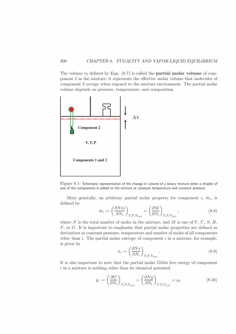
300 CHAPTER 8. FUGACITY AND VAPOR-LIQUID EQUILIBRIUM
The volume v2 defined by Eqn. (8.7) is called the partial molar volume of com-ponent 2 in the mixture; it represents the effective molar volume that molecules ofcomponent 2 occupy when exposed to the mixture environment. The partial molarvolume depends on pressure, temperature, and composition.
∆ V
V, T, P
Components 1 and 2
Component 2
Figure 8.1: Schematic representation of the change in volume of a binary mixture when a droplet ofone of the components is added to the mixture at constant temperature and constant pressure.
More generally, an arbitrary partial molar property for component i, mi, isdefined by
mi :=
(∂Nm
∂Ni
)
T,P,Nj 6=i
=
(∂M
∂Ni
)
T,P,Nj 6=i
, (8.8)
where N is the total number of moles in the mixture, and M is one of V , U , S, H,F , or G. It is important to emphasize that partial molar properties are defined asderivatives at constant pressure, temperature and number of moles of all componentsother than i. The partial molar entropy of component i in a mixture, for example,is given by
si :=
(∂Ns
∂Ni
)
T,P,Nj 6=i
. (8.9)
It is also important to note that the partial molar Gibbs free energy of componenti in a mixture is nothing other than its chemical potential
gi :=
(∂G
∂Ni
)
T,P,Nj 6=i
=
(∂Ng
∂Ni
)
T,P,Nj 6=i
= µi. (8.10)
301
For a single-component, or pure system, a partial molar quantity is just the specificquantity (e.g., vi = v for a pure system).
8.3.2 General Properties of Partial Molar Properties
To establish some of the useful properties of partial molar quantities, we beginby writing a differential of an arbitrary partial molar property mi. From Nm =M(T, P, Ni) we write
d(Nm) = N
(∂m
∂T
)
P,NjdT +N
(∂m
∂P
)
T,NjdP +
r∑
j=1
(∂Nm
∂Nj
)
T,P,Ni6=jdNj
= N
(∂m
∂T
)
P,NjdT +N
(∂m
∂P
)
T,NjdP +
r∑
j=1
mjdNj (8.11)
The left side of Eqn. (8.11) can be written as d(Nm) = mdN+Ndm. The differentialof Nj can be written as dNj = d(xjN) = xjdN + Ndxj . After substitution into(8.11) and rearrangement we arrive at
0 =
dm−(∂m
∂T
)
P,Nj
dT −(∂m
∂P
)
T,Nj
dP −r∑
j=1
mjdxj
N
+
m−q∑
j=1
mjxj
dN (8.12)
Equation (8.12) is a general thermodynamic expression; it is valid regardless of theparticular size N of the system, and is true for arbitrary values of the infinitesimalchange dN . These observations and Eqn. (8.12) can hold only if the bits inside thesquare brackets are each zero
dm =
(∂m
∂T
)
P,NjdT +
(∂m
∂P
)
T,NjdP +
r∑
j=1
mjdxj (8.13)
and,
m =
r∑
j=1
xjmj (8.14)
Eqn. (8.14) implies that the mixture value of an arbitrary property m can be ex-pressed as a sum of the corresponding partial molar properties mi weighted over themole fractions. In a sense, it is a rigorous generalization of Eqn. (8.5).
302 CHAPTER 8. FUGACITY AND VAPOR-LIQUID EQUILIBRIUM
For example, using Eqs. (8.10) and (8.14), the molar Gibbs free energy of amixture can be written as
g =r∑
j=1
µjxj . (8.15)
We can also simplify Eqn. (8.13). By recognizing that dm =∑q
j=1(mjdxj+xjdmj),Eqn. (8.13) can be rewritten as
0 =
(∂m
∂T
)
P,NjdT +
(∂m
∂P
)
T,NjdP −
r∑
j=1
xjdmj (8.16)
which is another version of the familiar Gibbs-Duhem equation; note, however, thatthe expression given here is more general than that derived earlier (i.e., Eqn. (3.22))because it is valid for an arbitrary property m. For the molar Gibbs free energy wehave
(∂g
∂T
)
P,Nj
dT +
(∂g
∂P
)
T,Nj
dP −r∑
j=1
xjdµj = 0 (8.17)
which, at constant temperature and pressure reduces to
r∑
j=1
xjdµj = 0, constant T and P . (8.18)
From Eqn. (8.18) we see that the chemical potentials of different species in a mixtureare not independent, but must change in a concerted manner. In general, Eqn. (8.16)indicates that all partial molar properties in a mixture are connected by Gibbs-Duhem type equations.
Example 8.3.1 From the measurement of a thermodynamic property for a binarymixture m(T, P, x1) at fixed T and P , but varying composition, find a simple graph-ical means to estimate the partial molar properties m1 and m2.
Solution: Since the experiments are accomplished at constant temperatureand pressure, it is convenient to begin with Eqn. (8.13), which becomes
dm =
2∑
i=1
midxi, fixed T, P
= m1dx1 + m2dx2, fixed T, P
= (m1 − m2) dx1, fixed T, P , (8.19)
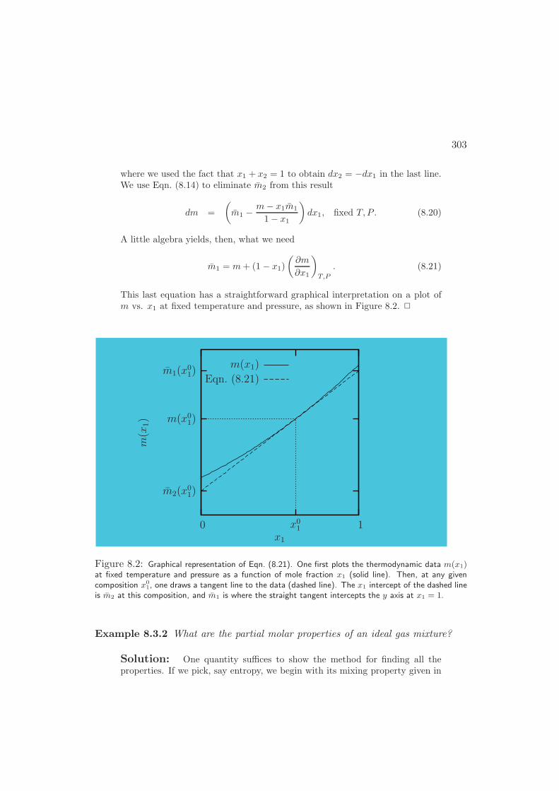
303
where we used the fact that x1 + x2 = 1 to obtain dx2 = −dx1 in the last line.We use Eqn. (8.14) to eliminate m2 from this result
dm =
(
m1 −m− x1m1
1− x1
)
dx1, fixed T, P . (8.20)
A little algebra yields, then, what we need
m1 = m+ (1 − x1)
(∂m
∂x1
)
T,P
. (8.21)
This last equation has a straightforward graphical interpretation on a plot ofm vs. x1 at fixed temperature and pressure, as shown in Figure 8.2. 2
Eqn. (8.21)
m(x1)
x1
m(x
1)
0 x01 1
m(x01)
m1(x01)
m2(x01)
Figure 8.2: Graphical representation of Eqn. (8.21). One first plots the thermodynamic data m(x1)at fixed temperature and pressure as a function of mole fraction x1 (solid line). Then, at any givencomposition x0
1, one draws a tangent line to the data (dashed line). The x1 intercept of the dashed lineis m2 at this composition, and m1 is where the straight tangent intercepts the y axis at x1 = 1.
Example 8.3.2 What are the partial molar properties of an ideal gas mixture?
Solution: One quantity suffices to show the method for finding all theproperties. If we pick, say entropy, we begin with its mixing property given in
304 CHAPTER 8. FUGACITY AND VAPOR-LIQUID EQUILIBRIUM
Eqs. (8.4), and multiply by the total number of moles N to make it extensiveto obtain
Sideal(T, P, xi) =∑
i
Nisideali (T, P )−R
∑
i
Ni log xi. (8.22)
Recall that the left side can be written as the mole-fraction-weighted sum ofthe partial molar quantities, using Eqn. (8.14)
∑
i
Nisideali (T, P, xi) =
∑
i
Ni[sideali (T, P )−R log xi
]. (8.23)
which gives us the expression for the partial molar entropy
sideali (T, P, xi) = sideali (T, P )−R log xi
= s0,i +
∫ T
T0
cidealv,i (T ′)
T ′dT ′ +R log
(TP0
xiPT0
)
. (8.24)
To obtain the second line, we used the expression for the entropy of a general-ized, pure ideal gas, Eqn. (3.17). Following the same procedure for the otherquantities yields the results
videali (T, P, xi) = videali (T, P ) =RT
P
uideali (T, P, xi) = uideali (T, P )
= u0,i +
∫ T
T0
cidealv,i (T ′)dT ′
hideali (T, P, xi) = hideali (T, P ) = uideali (T, P ) +RT
f ideali (T, P, xi) = uideali (T, P )− T sideali (T, P )
= f0,i − s0,i(T − T0) +
∫ T
T0
(T ′ − T
T ′
)
cidealv,i (T ′)dT ′
+RT log
(xiPT0P0T
)
gideali (T, P, xi) = f ideali (T, P ) +RT (8.25)
2
Example 8.3.3 Find the partial molar volume of an individual component of a gasmixture described by a virial equation of state.
Solution: In §7.4 we considered the virial equation of state from a molecularpoint of view. For the volume-explicit expansion, we discovered that the correctequation of state and mixing rules are
Z = 1 +BP
RT+ . . . (8.26)
305
whereB(T, Ni) =
∑
ij
xixjBij(T ) (7.43′)
Combining these expressions, and using the definition for the compressibilityfactor Z := PV/NRT , we obtain
V =NRT
P+
1
N
∑
ij
NiNjBij(T ). (8.27)
Following the definition of a partial molar property, we now take the derivativeof each side with respect to Nk to obtain
vk =
(∂V
∂Nk
)
T,P,Ni6=k
(8.28)
=RT
P+
1
N
∑
i
NiBik(T ) +1
N
∑
j
NjBkj(T )−1
N2
∑
ij
NiNjBik(T )
=RT
P+ 2
∑
i
xiBik(T )−B. (8.29)
To obtain the last line, we used the fact that Bij = Bji. 2
8.3.3 Residual Partial Molar Quantities
The result from Example 8.3.3 shows that the partial molar volume of real gasesdeviates from that of ideal gases. As it turns out, this deviation from ideality isextremely useful in defining fugacity and performing phase equilibria calculations.Hence, we define the residual partial molar properties
mRi (T, P, xi) := mi(T, P, xi)− mideal
i (T, P, xi), (8.30)
where m ≡ v, s, h, u, g, f as before. Note that we could just as well have defined thisquantity as the ‘partial molar residual’
mRi (T, P, xi) =
(∂MR
∂Ni
)
T,P,Nj 6=i, (8.31)
which is completely equivalent.From Example 8.3.3 we see that the residual partial molar volume predicted by
the virial equation of state is just vRk = 2∑
i xiBik(T )−B.
Example 8.3.4 Given a volume-explicit equation of state z(T, P, Ni), find theresidual partial molar Gibbs free energy.
306 CHAPTER 8. FUGACITY AND VAPOR-LIQUID EQUILIBRIUM
Solution: It is easier to use the alternative definition for the residual partialmolar Gibbs, Eqn. (8.31), since we already have an expression for the residualGibbs potential, Eqn. (4.67). Starting from the alternative definition
gRiRT
=
(∂
∂Ni
GR
RT
)
T,P,Nj 6=i
=∂
∂NiN
∫ P
0
[z(T, P ′, Nj)− 1]dP ′
P ′
=
∫ P
0
[zi(T, P′, Nj)− 1]
dP ′
P ′, (8.32)
where we have introduced the quantity
zi(T, P, Ni) :=(
∂
∂NiNz
)
T,P,Nj 6=i
(8.33)
Using this expression, the residual partial molar Gibbs free energy can be foundfor any volume-explicit equation of state when the appropriate mixing rules forthe parameters are known. 2
The results from the previous example are useful only for a volume-explicitequation of state for mixtures. More common are pressure-explicit equations ofstate. The analogous result for gRi given z(T, V, Ni) can be found from Eqn. (8.32)through a change of variable of integration from P to V . The result is
gRiRT
=
∫ ∞
V
[(∂
∂NiNz
)
T,V,Nj 6=i− 1
]
dV
V− log z. (8.34)
Pressure-explicit equations of state for mixtures are sometimes created from thosefor pure species, by having mixing rules for the parameters. For example, the vander Waals equation of state for mixtures arises by making the parameters a and bdepend upon some weighted sum of the pure-component values, such as given inEqn. (7.87).
8.4 Fugacity
We are finally in a position to define the fugacity; there are three main reasons forlearning it. First, it is ubiquitous in the technical literature. Second, it obviates theneed for fundamental relations to predict multicomponent vapor-liquid equilibriumcompositions. Third, it avoids difficulties at low pressures. What are these difficul-ties? Recall that all real gases behave ideally at low densities, and that the chemicalpotential of an ideal gas can be written in the form (see Eqn. (3.112))
µideali (T, P, xj) = µ0i (T ) +RT log (xiP ) . (8.35)
307
Hence, the chemical potential for gases goes to −∞ as the pressure goes to zero.
8.4.1 Definition of Fugacity
Because of the negative infinity in chemical potential at low pressures, it is usefulto subtract off the ideal part from the real part of the chemical potential, ratherlike a residual property. For example, each component of a liquid phase and vaporphase in equilibrium with each other at temperature T and pressure P must havethe same chemical potential in both phases
µliquidi (T, P, xliquidj ) = µvapori (T, P, xvaporj ). (8.36)
We would like to subtract off the ideal part—the part that goes to negative infinity—from each side. However, the liquid and the vapor phases are likely to have a differentcomposition, so we must be careful. For simplicity, we subtract off the chemicalpotential of the pure species at the same T and P from each side of this equation
µliquidi [xliquidj ]− µideal,purei = µvapori [xvaporj ]− µideal,purei . (8.37)
All the terms are at the same temperature and pressure, which we stop showingexplicitly here. Now we note that we can write the chemical potential for an idealmixture as µideali (xi) = µideal,purei + RT log(xi), Eqn. (8.4). Hence, the abovebecomes
µliquidi (xliquidj )− µideali (xliquidj ) +RT log(xliquidi ) =
µvapori (xvaporj )− µideali (xvaporj ) +RT log(xvapori ). (8.38)
We can utilize the fact that chemical potential is just the partial molar Gibbs freeenergy, and the definition for a residual property to write
[gRi (xliquidi )]liquid +RT log(xliquidi ) =
[gRi (xvaporj )]vapor +RT log(xvapori ). (8.39)
Or, if we divide each side by RT to make it dimensionless and take the exponential,we obtain
xliquidi exp
([gRi ]
liquid
RT
)
= xvapori exp
([gRi ]
vapor
RT
)
. (8.40)
This is our desired result, since we have eliminated the ideal contribution to thechemical potential, and found a quantity that must be equal in different phases atequilibrium. Historically, there is a slight modification to define fugacity which we
308 CHAPTER 8. FUGACITY AND VAPOR-LIQUID EQUILIBRIUM
also adopt; both sides of Eqn. (8.40) are multiplied by pressure, thereby giving thefollowing definition for the fugacity fi of component i in a mixture:
fi := xiP exp
(gRiRT
)
. (8.41)
Solving for the compositions of phases in equilibrium can be conveniently accom-plished by equating fugacities instead of chemical potentials. As we have just shown,equating fugacities is the same as equating chemical potentials, but the former re-quires only a PvT equation of state for the mixture.
8.4.2 Properties of fugacity
We can summarize some important properties of fugacity, two of which will requireproof.
1. Equal fugacities ⇔ equal chemical potentials.
2. At low densities, where real gases behave ideally (and the residual molar Gibbsfree energy vanishes), the fugacity becomes the so-called partial pressurexiP .
3. Equations of state are sometimes written for the fugacity coefficient φi,which is defined as
φi :=fixiP
. (8.42)
4. The pressure dependence of fugacity is
fi[T, P2] = fi[T, P1] exp
[∫ P2
P1
vi[T, P′]
RTdP ′]
. (8.43)
This form is particularly useful for measuring fugacity of pure systems.
5. The temperature dependence of fugacity is
fi[T2, P ] = fi[T1, P ] exp
[
−∫ T2
T1
hRi [T′, P ]
RT ′2 dT ′]
. (8.44)
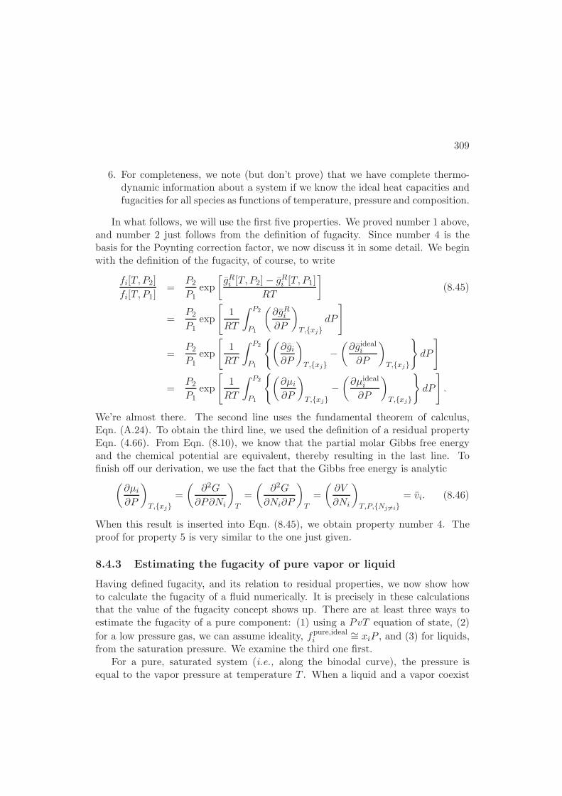
309
6. For completeness, we note (but don’t prove) that we have complete thermo-dynamic information about a system if we know the ideal heat capacities andfugacities for all species as functions of temperature, pressure and composition.
In what follows, we will use the first five properties. We proved number 1 above,and number 2 just follows from the definition of fugacity. Since number 4 is thebasis for the Poynting correction factor, we now discuss it in some detail. We beginwith the definition of the fugacity, of course, to write
fi[T, P2]
fi[T, P1]=
P2
P1exp
[gRi [T, P2]− gRi [T, P1]
RT
]
(8.45)
=P2
P1exp
[
1
RT
∫ P2
P1
(∂gRi∂P
)
T,xjdP
]
=P2
P1exp
[
1
RT
∫ P2
P1
(∂gi∂P
)
T,xj−(∂gideali
∂P
)
T,xj
dP
]
=P2
P1exp
[
1
RT
∫ P2
P1
(∂µi∂P
)
T,xj−(∂µideali
∂P
)
T,xj
dP
]
.
We’re almost there. The second line uses the fundamental theorem of calculus,Eqn. (A.24). To obtain the third line, we used the definition of a residual propertyEqn. (4.66). From Eqn. (8.10), we know that the partial molar Gibbs free energyand the chemical potential are equivalent, thereby resulting in the last line. Tofinish off our derivation, we use the fact that the Gibbs free energy is analytic
(∂µi∂P
)
T,xj=
(∂2G
∂P∂Ni
)
T
=
(∂2G
∂Ni∂P
)
T
=
(∂V
∂Ni
)
T,P,Nj 6=i= vi. (8.46)
When this result is inserted into Eqn. (8.45), we obtain property number 4. Theproof for property 5 is very similar to the one just given.
8.4.3 Estimating the fugacity of pure vapor or liquid
Having defined fugacity, and its relation to residual properties, we now show howto calculate the fugacity of a fluid numerically. It is precisely in these calculationsthat the value of the fugacity concept shows up. There are at least three ways toestimate the fugacity of a pure component: (1) using a PvT equation of state, (2)
for a low pressure gas, we can assume ideality, fpure,ideali∼= xiP , and (3) for liquids,
from the saturation pressure. We examine the third one first.For a pure, saturated system (i.e., along the binodal curve), the pressure is
equal to the vapor pressure at temperature T . When a liquid and a vapor coexist
310 CHAPTER 8. FUGACITY AND VAPOR-LIQUID EQUILIBRIUM
at equilibrium, the chemical potentials of the two phases are equal; from propertynumber 1 of fugacities we have
fvapor[P sat, vvapor] = f liquid[P sat, vliquid]. (8.47)
The quantities in the square brackets serve to remind us that the fugacity of thevapor is to be evaluated at the vapor pressure and at the saturated vapor molarvolume, and that of the liquid is to be evaluated at the saturated liquid molarvolume.
Using property number 4, Eqn. (8.43), the fugacity of a pure condensed phase(a liquid or a solid) at temperature T and arbitrary pressure P can therefore beexpressed by
fpurei [P ] = fpure, vapori [P sat] exp
[∫ P
P sat
v[T, P ′]RT
dP ′]
, (8.48)
where v[T, P ′] is now the molar volume of a condensed phase at pressure P ′.The path outlined above to calculate the fugacity of a condensed fluid is illus-
trated in Figure (8.3), which provides a schematic representation of a subcriticalisotherm and the coexistence curve of a simple fluid in the P − v plane. To evaluatethe fugacity of the fluid at point A, we follow the isotherm up to point B, andcalculate the corresponding change in the liquid-phase fugacity according to:
fpurei [P ] = fpure, liquidi [P sat] exp
[∫ P
P sat
vliquid[T, P ′]RT
dP ′]
, (8.49)
Since, according to Eqn. (8.47), the fugacity of a pure fluid at point B is the same
as that at point C, we can replace f liquidi [P sat] in Eqn. (8.49) with fvapori [P sat] toarrive at Eqn. (8.48).
Eqn. (8.48) is of little use unless we can determine fvapori at P sat. We recallthat, at the binodal (or coexistence) curve, the fluid can behave rather non-ideally.However, for the moment, it suffices to point out that the vapor pressure of a solidor a liquid is usually relatively small; at such low pressures, within engineeringapproximation, most vapors are not too far away from ideal-gas behavior. Theassumption fvapor[P sat] ≈ P sat is therefore justified, and Eqn. (8.48) can be writtenas
fi[T, P ] ≈ P sat(T ) exp
[∫ P
P sat
v[T, P ′]RT
dP ′]
︸ ︷︷ ︸
Poynting Correction Factor
, ideal vapor phase. (8.50)
The physical meaning of a fugacity is now apparent: it is a vapor pressure correctedfor the effect of pressure on the condensed phase. By introducing fugacity, we are
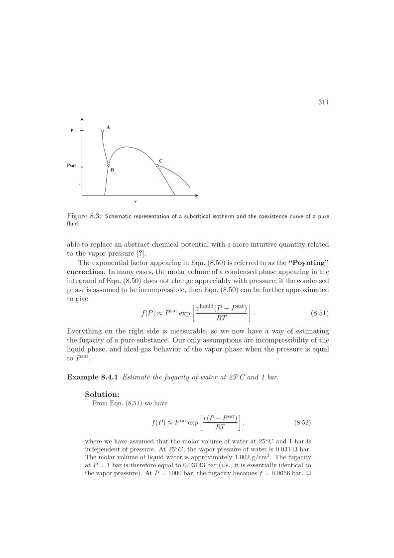
311
P
Psat
A
B
C
v
Figure 8.3: Schematic representation of a subcritical isotherm and the coexistence curve of a purefluid.
able to replace an abstract chemical potential with a more intuitive quantity relatedto the vapor pressure [?].
The exponential factor appearing in Eqn. (8.50) is referred to as the “Poynting”correction. In many cases, the molar volume of a condensed phase appearing in theintegrand of Eqn. (8.50) does not change appreciably with pressure; if the condensedphase is assumed to be incompressible, then Eqn. (8.50) can be further approximatedto give
f [P ] ≈ P sat exp
[vliquid(P − P sat)
RT
]
. (8.51)
Everything on the right side is measurable, so we now have a way of estimatingthe fugacity of a pure substance. Our only assumptions are incompressibility of theliquid phase, and ideal-gas behavior of the vapor phase when the pressure is equalto P sat.
Example 8.4.1 Estimate the fugacity of water at 25C and 1 bar.
Solution:From Eqn. (8.51) we have
f(P ) ≈ P sat exp
[v(P − P sat)
RT
]
, (8.52)
where we have assumed that the molar volume of water at 25C and 1 bar isindependent of pressure. At 25C, the vapor pressure of water is 0.03143 bar.The molar volume of liquid water is approximately 1.002 g/cm3. The fugacityat P = 1 bar is therefore equal to 0.03143 bar (i.e., it is essentially identical tothe vapor pressure). At P = 1000 bar, the fugacity becomes f = 0.0656 bar. 2
312 CHAPTER 8. FUGACITY AND VAPOR-LIQUID EQUILIBRIUM
Our second method for estimating the fugacity of a pure system uses a PvTequation of state. Note that the definition for fugacity, Eqn. (8.41), simplifies for apure system, since gRi ≡ gR, when pure. Hence, we can use the relations for residualproperties derived in §4.4.2 to find gR from any given PvT relation. This integralhas been performed for many of the models given in Appendix B, and expressions forthe pure fugacities can be found there. The following example shows the procedurefor a volume-explicit virial equation of state.
Example 8.4.2 Derive an expression for the fugacity coefficient of a fluid describedby a volume-explicit virial equation of state truncated after the second term.
Solution: From Eqn. (8.54) and the compressibility factor of a virial gas,namely z = 1 + BP
RT , we have
logφ =
∫ P
0
1 + BPRT − 1
PdP, constant T
=BP
RT. (8.53)
2
Expressions for models valid over greater ranges of density than the virial ex-pansion give more complex mathematical expressions. The following example testsone of the assumptions in the previous method.
Example 8.4.3 Use the Peng-Robinson model to predict the fugacity of methanolat its saturation pressure and 80C.
Solution: We can find the critical properties for methanol from the NISTChemistry Webbook to be Tc = 513 ± 1K and Pc = 81 ± 1bar. The reducedtemperature is thus Tr = T/Tc = (273 + 80)/513 = 0.688. For this reducedtemperature, we can estimate the saturation pressure of methanol using theAntoine-like equation found from the Peng-Robinson model, Eqn. (B.55). Theexpression requires the acentric factor for methanol, which we find from fromTable D.3 to be ω = 0.272. Hence, we find B = −7.13465, C = −3.07399,and D = −19.249. Therefore, from Eqn. (B.55) we find the reduced saturationpressure to be 0.0447, or P sat ∼= 3.62bar.
To find the fugacity, we use Eqn. (B.54). Note that this expression requiresthe temperature and specific volume, whereas we have the temperature and thepressure. To find the specific volume, we first need the parameters, which wecan find from Eqs. (B.49)
a0 ≈ 0.4572367(RTc)
2
Pc= 10.2698 l2 · bar/mol
2,
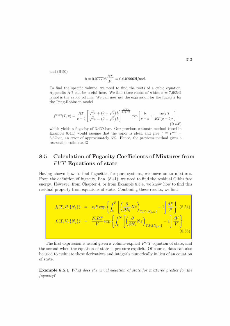
313
and (B.50)
b ≈ 0.077796RTcPc
= 0.0409662l/mol.
To find the specific volume, we need to find the roots of a cubic equation.Appendix A.7 can be useful here. We find three roots, of which v = 7.68541l/mol is the vapor volume. We can now use the expression for the fugacity forthe Peng-Robinson model
fpure(T, v) =RT
v − b
[√2v +
(2 +
√2)b√
2v −(2−
√2)b
] a(T )
2√
2RT
exp
[b
v − b+
va(T )
RT (v − b)2
]
.
(B.54′)which yields a fugacity of 3.439 bar. Our previous estimate method (used inExample 8.4.1) would assume that the vapor is ideal, and give f ∼= P sat =3.62bar, an error of approximately 5%. Hence, the previous method gives areasonable estimate. 2
8.5 Calculation of Fugacity Coefficients of Mixtures fromPV T Equations of state
Having shown how to find fugacities for pure systems, we move on to mixtures.From the definition of fugacity, Eqn. (8.41), we need to find the residual Gibbs freeenergy. However, from Chapter 4, or from Example 8.3.4, we know how to find thisresidual property from equations of state. Combining these results, we find
fi(T, P, Nj) = xiP exp
∫ P
0
[(∂
∂NiNz
)
T,P,Nj 6=i− 1
]
dP
P
(8.54)
fi(T, V, Nj) =NiRT
Vexp
∫ ∞
V
[(∂
∂NiNz
)
T,V,Nj 6=i− 1
]
dV
V
(8.55)
The first expression is useful given a volume-explicit PV T equation of state, andthe second when the equation of state is pressure explicit. Of course, data can alsobe used to estimate these derivatives and integrals numerically in lieu of an equationof state.
Example 8.5.1 What does the virial equation of state for mixtures predict for thefugacity?
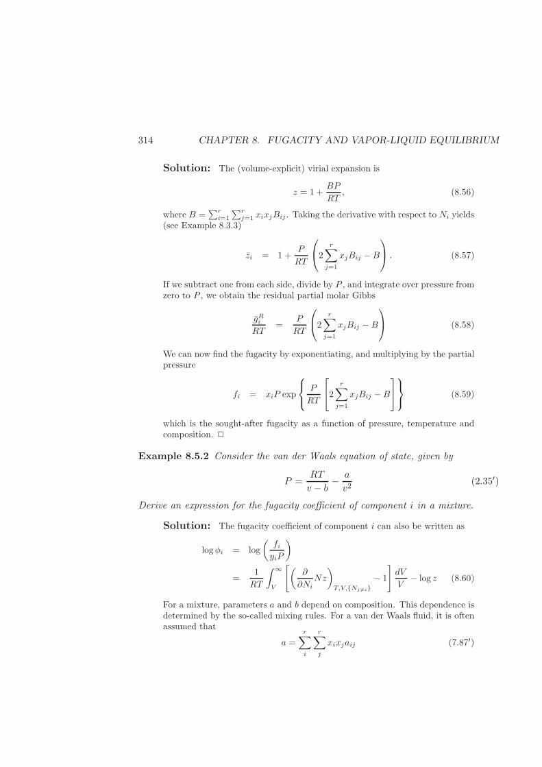
314 CHAPTER 8. FUGACITY AND VAPOR-LIQUID EQUILIBRIUM
Solution: The (volume-explicit) virial expansion is
z = 1 +BP
RT, (8.56)
where B =∑ri=1
∑rj=1 xixjBij . Taking the derivative with respect to Ni yields
(see Example 8.3.3)
zi = 1 +P
RT
2
r∑
j=1
xjBij −B
. (8.57)
If we subtract one from each side, divide by P , and integrate over pressure fromzero to P , we obtain the residual partial molar Gibbs
gRiRT
=P
RT
2
r∑
j=1
xjBij −B
(8.58)
We can now find the fugacity by exponentiating, and multiplying by the partialpressure
fi = xiP exp
P
RT
2
r∑
j=1
xjBij −B
(8.59)
which is the sought-after fugacity as a function of pressure, temperature andcomposition. 2
Example 8.5.2 Consider the van der Waals equation of state, given by
P =RT
v − b− a
v2(2.35′)
Derive an expression for the fugacity coefficient of component i in a mixture.
Solution: The fugacity coefficient of component i can also be written as
logφi = log
(fiyiP
)
=1
RT
∫ ∞
V
[(∂
∂NiNz
)
T,V,Nj 6=i
− 1
]
dV
V− log z (8.60)
For a mixture, parameters a and b depend on composition. This dependence isdetermined by the so-called mixing rules. For a van der Waals fluid, it is oftenassumed that
a =
r∑
i
r∑
j
xixjaij (7.87′)
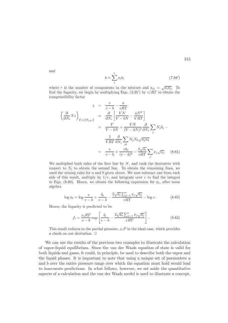
315
and
b =
r∑
i
xibi (7.88′)
where r is the number of components in the mixture and aij =√aiaj . To
find the fugacity, we begin by multiplying Eqn. (2.35′) by v/RT to obtain thecompressibility factor
z =v
v − b− a
vRT(
∂
∂NiNz
)
T,v,Nj 6=i
=∂
∂Ni
[V N
V − bN− aN2
V RT
]
=V
V − bN+
V N
(V − bN)2∂
∂Ni
∑
j
Njbj −
1
V RT
∂
∂Ni
∑
jk
NjNk√ajak
=v
v − b+
vbi(v − b)2
− 2√ai
vRT
∑
j
xj√aj . (8.61)
We multiplied both sides of the first line by N , and took the derivative withrespect to Ni to obtain the second line. To obtain the remaining lines, weused the mixing rules for a and b given above. We now subtract one from eachside of this result, multiply by 1/v, and integrate over v to find the integralin Eqn. (8.60). Hence, we obtain the following expression for φi, after somealgebra
log φi = logv
v − b+
biv − b
−2√ai∑r
j=1 xj√aj
vRT− log z. (8.62)
Hence, the fugacity is predicted to be
fi =xiRT
v − bexp
[
biv − b
−2√ai∑rj=1 xj
√aj
vRT
]
. (8.63)
This result reduces to the partial pressure, xiP in the ideal case, which providesa check on our derivation. 2
We can use the results of the previous two examples to illustrate the calculationof vapor-liquid equilibrium. Since the van der Waals equation of state is valid forboth liquids and gases, it could, in principle, be used to describe both the vapor andthe liquid phases. It is important to note that using a unique set of parameters aand b over the entire pressure range over which the equation must hold would leadto inaccurate predictions. In what follows, however, we set aside the quantitativeaspects of a calculation and the van der Waals model is used to illustrate a concept.
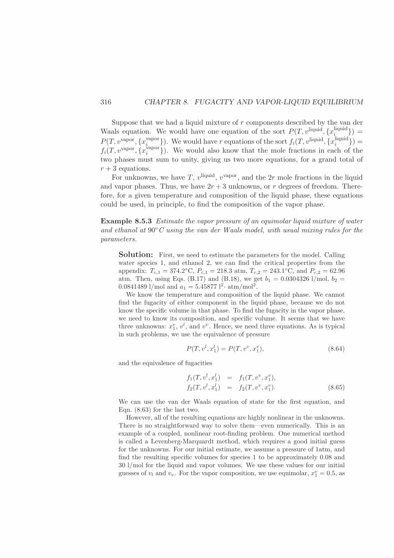
316 CHAPTER 8. FUGACITY AND VAPOR-LIQUID EQUILIBRIUM
Suppose that we had a liquid mixture of r components described by the van derWaals equation. We would have one equation of the sort P (T, vliquid, xliquidi ) =
P (T, vvapor, xvapori ). We would have r equations of the sort fi(T, vliquid, xliquidi ) =
fi(T, vvapor, xvapori ). We would also know that the mole fractions in each of the
two phases must sum to unity, giving us two more equations, for a grand total ofr + 3 equations.
For unknowns, we have T , vliquid, vvapor, and the 2r mole fractions in the liquidand vapor phases. Thus, we have 2r+3 unknowns, or r degrees of freedom. There-fore, for a given temperature and composition of the liquid phase, these equationscould be used, in principle, to find the composition of the vapor phase.
Example 8.5.3 Estimate the vapor pressure of an equimolar liquid mixture of waterand ethanol at 90C using the van der Waals model, with usual mixing rules for theparameters.
Solution: First, we need to estimate the parameters for the model. Callingwater species 1, and ethanol 2, we can find the critical properties from theappendix: Tc,1 = 374.2C, Pc,1 = 218.3 atm, Tc,2 = 243.1C, and Pc,2 = 62.96atm. Then, using Eqs. (B.17) and (B.18), we get b1 = 0.0304326 l/mol, b2 =0.0841489 l/mol and a1 = 5.45877 l2· atm/mol2.
We know the temperature and composition of the liquid phase. We cannotfind the fugacity of either component in the liquid phase, because we do notknow the specific volume in that phase. To find the fugacity in the vapor phase,we need to know its composition, and specific volume. It seems that we havethree unknowns: xv1 , v
l, and vv. Hence, we need three equations. As is typicalin such problems, we use the equivalence of pressure
P (T, vl, xl1) = P (T, vv, xv1), (8.64)
and the equivalence of fugacities
f1(T, vl, xl1) = f1(T, v
v, xv1),
f2(T, vl, xl1) = f2(T, v
v, xv1). (8.65)
We can use the van der Waals equation of state for the first equation, andEqn. (8.63) for the last two.
However, all of the resulting equations are highly nonlinear in the unknowns.There is no straightforward way to solve them—even numerically. This is anexample of a coupled, nonlinear root-finding problem. One numerical methodis called a Levenberg-Marquardt method, which requires a good initial guessfor the unknowns. For our initial estimate, we assume a pressure of 1atm, andfind the resulting specific volumes for species 1 to be approximately 0.08 and30 l/mol for the liquid and vapor volumes. We use these values for our initialguesses of vl and vv. For the vapor composition, we use equimolar, xv1 = 0.5, as
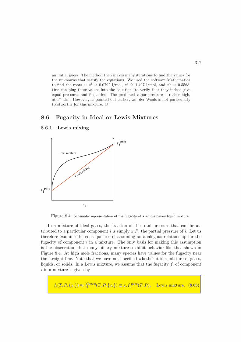
317
an initial guess. The method then makes many iterations to find the values forthe unknowns that satisfy the equations. We used the software Mathematicato find the roots as vl ∼= 0.0792 l/mol, vv ∼= 1.497 l/mol, and xv1
∼= 0.5568.One can plug these values into the equations to verify that they indeed giveequal pressures and fugacities. The predicted vapor pressure is rather high,at 17 atm. However, as pointed out earlier, van der Waals is not particularlytrustworthy for this mixture. 2
8.6 Fugacity in Ideal or Lewis Mixtures
8.6.1 Lewis mixing
f
x
i
i
pure
f j pure
Lewis
mix
ing
real mixture
Figure 8.4: Schematic representation of the fugacity of a simple binary liquid mixture.
In a mixture of ideal gases, the fraction of the total pressure that can be at-tributed to a particular component i is simply xiP , the partial pressure of i. Let ustherefore examine the consequences of assuming an analogous relationship for thefugacity of component i in a mixture. The only basis for making this assumptionis the observation that many binary mixtures exhibit behavior like that shown inFigure 8.4. At high mole fractions, many species have values for the fugacity nearthe straight line. Note that we have not specified whether it is a mixture of gases,liquids, or solids. In a Lewis mixture, we assume that the fugacity fi of componenti in a mixture is given by
fi(T, P, xi) ≈ fLewisi (T, P, xi) ≡ xifi
pure(T, P ), Lewis mixture, (8.66)
318 CHAPTER 8. FUGACITY AND VAPOR-LIQUID EQUILIBRIUM
where fipure is used to denote the fugacity of pure component i and xi is its con-
centration in the mixture. As we will show, the results of assumption Eqn. (8.66)are mixing properties reminiscent of those of ideal gases. The physical implicationsare quite different. Recall that the molecules of an ideal gas do not interact. ALewis mixture, on the other hand, has molecular interactions, but assumes that theinteraction between two different molecules are the same as between two of the samemolecules.
The relation given by (8.66) is often referred to as Lewis’ fugacity rule, and itis used to define what is usually called an ideal mixture. Again, it is emphasizedthat in order to avoid confusion with ideal-gas mixtures, however, we refer to sucha system as a Lewis mixture.
8.6.2 Properties of Lewis (Ideal) Mixtures
Recalling the definition of fugacity coefficient, we can write
φLewisi =
fLewisi
xiP=fpurei
P= φpurei . (8.67)
We shall see in the next chapter that, since the fugacity coefficient is just that ofthe pure component, Lewis mixing always predicts miscibility. Given the physicalbasis for Lewis mixing, this observation is expected.
Lewis’ fugacity rule leads to several important consequences for the propertiesof a mixture. Specifying the fugacity of a component has implications about thechemical potential of that component, as we will now prove. Since the Gibbs freeenergy is the sum of the chemical potentials, according to Eqn. (8.15), we can write
g(T, P, xi) =∑
i
xiµi
=∑
i
xigi
=∑
i
xi
[
gRi + gideali
]
=∑
i
xi
[
RT log
(fixiP
)
+ gideali
]
. (8.68)
To obtain the second line we used the equivalence between partial molar Gibbs freeenergy and chemical potential, Eqn. (8.10). To get to the third line, we used thedefinition of a residual property. The last line comes from the definition of fugacity,
319
Eqn. (8.41). Hence, for a Lewis mixture we can write
gLewis(T, P, xi) =∑
i
xi
[
RT log
(fLewisi
xiP
)
+ gideali
]
.
=∑
i
xi
[
RT log
(fpurei
P
)
+ gideali
]
.
=∑
i
xi
[
(gRi )pure + gideali
]
.
=∑
i
xi
[
gpurei − gpure,ideali + gideali
]
.
=∑
i
xi [gpurei +RT log xi] . (8.69)
This last relation is something like a fundamental relation, although it requires thatwe have fundamental relations for each of the pure species. This lengthy derivation isimportant, only because we wish to derive several more interesting relations. Theseinteresting relations are the characteristic mixing properties of a Lewis mixture,which we summarize here
vLewis(T, P, xi) =
r∑
i=1
xivpurei (T, P ) (8.70)
uLewis(T, P, xi)RT
=1
RT
r∑
i=1
xiupurei (T, P ) (8.71)
hLewis(T, P, xi)RT
=1
RT
r∑
i=1
xihpurei (T, P ) (8.72)
sLewis(T, P, xi)R
=1
R
r∑
i=1
xispurei (T, P )−
r∑
i=1
xi log(xi) (8.73)
fLewis(T, P, xi)RT
=1
RT
r∑
i=1
xifpurei (T, P ) +
r∑
i=1
xi log(xi) (8.74)
gLewis(T, P, xi)RT
=1
RT
r∑
i=1
xigpurei (T, P ) +
r∑
i=1
xi log(xi) (8.75)
µLewisi (T, P, xi)
RT=
µpurei (T, P )
RT+ log(xi) (8.76)
320 CHAPTER 8. FUGACITY AND VAPOR-LIQUID EQUILIBRIUM
It is interesting to note that, while the volume and the enthalpy of a Lewismixture are given by a simple linear combination of pure component properties,the molar entropy and Gibbs free energy are not. Earlier in this section, a sim-ple, intuitive explanation was provided as to why Equation (8.70) might be validfor mixtures of similar components. The precise form of the additional “mixing”contributions that arise in the Lewis Gibbs free energy and entropy expressions areperhaps less intuitive, but one can use simple arguments to discuss why they haveto be there. If two similar components are mixed, the resulting solution is likelyto be homogeneous; the mixing process occurs spontaneously, without a need forexternal work. The converse is not true; the mixture does not separate into its pureconstituents by itself. In order to occur spontaneously, the mixing process must leadto an increase of the entropy of the system. The (−∑r
i xi lnxi) term in Eqn. (8.73)is always positive; it is this term that renders the entropy of the mixture higher thanthat of the original, “unmixed” system of pure components.
Note also that these results are similar in form to those for mixing general idealgases, shown in §8.2. There is an essential difference, however: Lewis mixing rulescan be applied to real gases, even liquids. But, these apply only when the species arevery similar; if the mixture evolves heat upon mixing, such as happens when mixingsulfuric acid and water, then the mixture is clearly not Lewis. Or, if the mixturechanges volume, or is immiscible, then use of the Lewis mixing approximation is abad idea.
8.6.3 A Simple Application of Ideal Mixing: Raoult’s Law
Consider a vessel containing a vapor phase (′) in equilibrium with a liquid phase (′′).We wish to find a relation between the vapor and liquid phase compositions, say topredict the bubble point of a mixture. The composition of the vapor phase is givenby yi, and that of the liquid phase is given by xi. From Eqn. (8.1) we knowthat, at equilibrium, the chemical potential of each component is the same in bothphases; from the definition of fugacity, Eqn. (8.41), such equality can be expressedas
f ′i = f ′′i , i = 1, ..., r (8.77)
If we now assume that the vapor phase (denoted by superscript ′) consists of amixture of ideal gases, we have
f ′i = yifipure ideal gas i = 1, ..., r ideal gas, (8.78)
or, recalling that the fugacity of an ideal gas is the pressure
f ′i = yiP i = 1, ..., r ideal gas. (8.79)
321
If we assume that the liquid phase (denoted by superscript ′) is a Lewis mixture of liq-
uids (i.e., if we invoke Lewis’ fugacity rule, Eqn. (8.66)), we have f ′′i = xifpure liquidi .
Eqn. (8.77) therefore leads to
yiP = xifipure liquid, i = 1, ..., r. (8.80)
We are now faced with the problem of calculating the fugacity of a pure liquidfi
pure liquid. If we also assume that the volume of the liquid v is constant in therange P sat to P , we get Eqn. (8.51), that is
f(P ) ≈ P sat exp
[v(P − P sat)
RT
]
, incompressible liquid, ideal vapor.
Since the molar volume of a liquid is usually much smaller than that of a vapor, atmoderate pressures the Poynting correction is negligible and can be omitted fromapproximate calculations. In that case, f(P ) ≈ P sat and Eqn. (8.80) can be writtenas
yiP ≈ xiPsati , i = 1, ..., r (8.81)
• The vapor consists of a mixture of ideal gases
• The liquid phase is a Lewis (or ideal) mixture; it therefore adheres toLewis’ fugacity rule.
• The pressure is moderate and the Poynting correction can therefore beneglected.
All of the assumptions that have gone into formulating Eqn. (8.81) are listed. Theresult is known as Raoult’s “law”. It provides a simple means for conductingvapor-liquid equilibria calculations for mixtures of fluids. Bear in mind, however,that the approximations that were made to derive Raoult’s law are severe, and itsapplicability is therefore highly limited.
Raoult’s law can be used to illustrate the calculation of simple vapor-liquidphase diagrams for binary mixtures. Consider a vapor mixture of composition yi, ata temperature T . If we wish to determine the pressure at which the mixture startsto condense, the so-called dew pressure, we can simply write
y1P = x1Psat1
y2P = x2Psat2 . (8.82)
322 CHAPTER 8. FUGACITY AND VAPOR-LIQUID EQUILIBRIUM
The sum of these two equations leads to the sought after expression for the pressure:
P = x1Psat1 + x2P
sat2 . (8.83)
The composition of the first drop of liquid that appears can now be determinedaccording to
yi =xiP
sati
P.
By repeating this procedure for the entire range of composition from y1 = 0 toy1 = 1, the entire dew curve can be generated. The so-called “bubble pressure”,which represents the pressure at which a liquid mixture starts to vaporize, can becalculated in an analogous manner. As illustrated in the next few sections, thecalculation of vapor-liquid coexistence becomes slightly more cumbersome when thevapor or liquid phase cannot be assumed to behave as ideal gases or Lewis mixtures.In that case, it is necessary to resort to iterative procedures, but the basic structureof the problem remains unchanged.
8.7 Solubility of Solids and Liquids in Compressed Gases
8.7.1 Phase Equilibria Between a Solid and a Compressed Gas
The equations for phase equilibria discussed in this chapter are generally applicable,regardless of whether the phases under consideration are solid, liquid, or gaseous.In this section, we briefly discuss their application to solid-fluid equilibria.
In recent years, the extraction of solids using compressed gases has attractedconsiderable attention. In the food industry, for example, it is now common toextract particular substances (e.g., caffeine from coffee or alcohol from beer) usinghigh-pressure gases such as carbon dioxide. In the environmental industry, there areprocesses to remove pollutants from soil, also using carbon dioxide. It is thereforeuseful to discuss briefly the application of thermodynamics for the design of suchprocesses.
For equilibrium between a pure solid and a pure gas phase, Eqn. (8.47) can bewritten in the following form
f solid[P sat] = fgas[P sat] (8.84)
where the fugacities are evaluated at the vapor pressure of the system. For a mixture,we write
f solidi = fgasi , i = 1, ..., r (8.85)
For simplicity, we assume that the solid phase under consideration is a pure sub-stance; in most cases, the solubility of the other gases in the solid is sparingly small
323
and this is a reasonable assumption. In that event, the fugacity of the solid is givenby
f solidi ≈ fpure solidi = φsati P sat
i exp
(∫ P
P sat
vsolidi
RTdP
)
, constant T (8.86)
where φsati is the fugacity coefficient of pure i evaluated at pressure P sat, and vsolidi
is the molar volume of pure solid i.The fugacity in the vapor phase is calculated from either Eqn. (8.54) or (8.55).
Typically, however, one writes this in terms of the fugacity coefficient
fi = yiφiP. (8.87)
After substitution of Eqs. (8.87) and (8.86) into (8.85), we arrive at an expressionfor the solubility of the solid, component i, in the compressed-gas phase
yiφi(T, P, yi)P = φsati P sati exp
(∫ P
P sat
vsolidi
RTdP
)
, (8.88)
where it is understood that φi is found from Eqn. (8.54) or (8.55). Note that it isnot possible, in general, to find an explicit expression for yi.
8.7.2 Phase Equilibria Between a Liquid and a Compressed Gas
The situation for a liquid phase in equilibrium with a compressed gas is slightlymore complicated, as the compressed gas is likely to be soluble in the liquid. In thissection we only discuss the case in which the solubility of the gas in the liquid is nottoo high. This is often the case in applications.
Figure 8.4 illustrates schematically the expected behavior of the fugacity of com-ponent 1 in a binary mixture. If the two components were miscible in all proportions,the fugacity would follow a behavior similar to that depicted in the figure. From theshape of that curve, it is clear that assuming Lewis mixing is only reasonable whenthe component under consideration is fairly concentrated, almost pure. On the otherhand, assuming Lewis mixing for a dilute component results in considerable errors.
To circumvent this problem, it is possible to define a new type of mixing thatwill be accurate for dilute components; in close analogy to Lewis mixtures, for dilutecomponents we introduce Henry’s Law
fi ∼= fHenryi := xiHi,j(T, P ) (8.89)
where Hi,j is the Henry’s constant for component i in the solvent, component j,
and where fHenryi is a fugacity in the Henry’s-law limit of vanishing concentration.
324 CHAPTER 8. FUGACITY AND VAPOR-LIQUID EQUILIBRIUM
Henry’s constants depend on both temperature and pressure. They have been mea-sured for many gases dissolved in a wide variety of liquids. Note, however, that theseconstants are often measured at low to moderate pressures. In order to extrapolateto high pressures, we can use property 4 of fugacities. By substitution of Eqn. (8.89)into (8.43), we get
Hi,j[T, P2] = Hi,j[T, P1] exp
[∫ P2
P1
v∞i [T, P ′]RT
dP ′]
. (8.90)
where the superscript ∞ denotes a quantity evaluated at infinite dilution.
We can now return to the general expressions for phase equilibria between aliquid and a vapor, and write
f liquidi = fgasi i = 1, ..., r (8.91)
For the liquid phase we use Eqn. (8.90), and for the vapor phase we use Eqn. (8.49).The solubility of the solvent j in the compressed gas phase is therefore given by
yjφj(T, P, yj)P = xjPsatj φsatj exp
(∫ P
P satj
vjRT
dP
)
(8.92)
where the solubility of component i in the liquid phase is given by
xi =yiφiP
Hi,j exp(∫ P
P satj
v∞iRT dP
) (8.93)
8.8 Summary
In this chapter we introduced the quantity called fugacity , which plays a centralrole in calculating multicomponent vapor-liquid equilibrium. Instead of equatingchemical potentials to find compositions of different phases, we equate fugacities.Several ways of measuring and predicting fugacities were spelled out in the chapter.These methods are briefly summarized here.
• We defined a partial molar quantity by the relation
mi :=
(∂Nm
∂Ni
)
T,P,Nj 6=i
=
(∂M
∂Ni
)
T,P,Nj 6=i
, (8.8)

325
• Fugacity was defined by
fi := xiP exp
(gRiRT
)
, (8.41)
where gRi is the residual partial molar Gibbs free energy for species i. Fiveimportant properties of the fugacity were given in §8.4.2.
• When two phases (1) and (2) are in equilibrium, then they have the sametemperature and pressure, and each component has the same fugacity
T (1) = T (2)
P (1) = P (2)
f(1)i = f
(2)i , i = 1, 2, . . . , r
• For systems with low vapor pressure, we can estimate the fugacity of a pure(nearly incompressible) liquid from
f [T, P ] ≈ P sat[T ] exp
[vliquid(P − P sat)
RT
]
. (8.51)
• We know how to predict fugacities from either pressure-explicit or volume-explicit equations of state for mixtures, from
fi(T, P, Nj) = xiP exp
∫ P
0
[(∂
∂NiNz
)
T,P,Nj 6=i− 1
]
dP
P
(8.54)
fi(T, V, Nj) =NiRT
Vexp
∫ ∞
V
[(∂
∂NiNz
)
T,V,Nj 6=i− 1
]
dV
V
. (8.55)
• Lewis mixing approximates fugacities of individual components of a mixturein terms of their values in the pure state
fi ≈ fLewisi := xifi
pure. (8.66)
This approximation is typically valid for liquid species in high concentration.Raoult’s law is a special case, where Lewis mixing is assumed for the liquid,the Poynting correction is neglected, and the vapor phase is assumed to be anideal gas.
326 CHAPTER 8. FUGACITY AND VAPOR-LIQUID EQUILIBRIUM
• For liquid species in low concentration, Henry’s Law is more useful than Lewismixing
fHenryi := xiHi,j, (8.89)
where Hi,j is called Henry’s Law constant for dilute species i in concentratedspecies j.
By the end of this chapter, the student should be able to calculate fugacities forpure components at arbitrary temperature and pressure using any equation of state.Also, the student should be able to devise experiments to estimate fugacities fromexperiments, and predict temperature and pressure dependence.
Given a fundamental relation for mixtures, the student should be able to estimatefugacities. Typically, these are models for pure substances (e.g., Peng-Robinson)with ‘mixing rules’ for the parameters.
327
8.9 Exercises
8.3.A Derive Eqn. (8.34) by changing the variable of integration in Eqn. (8.32).Hint: You might find it useful to prove first that
(∂
∂NiNz
)
T,P,Nj 6=i= −zNRT
V 2
(∂
∂NiNz
)
T,V,Nj 6=i
(∂V
∂P
)
T,Ni
8.4.A: Calculate the fugacity of hexane at 25C and at 1 and 50 bar.
8.4.B: Calculate the fugacity of mono-ethanol-amine (MEA) at 50C and at 1 and50 bar.
8.4.C: Calculate the fugacity of acetone at 50C and at 1 and 50 bar.
8.4.D: Show that the effects of pressure and temperature on the fugacity coefficientare given by
(∂ log φ
∂P
)
T,N
=vR
RT(8.94)
and (∂ log φ
∂T
)
P,N
= − hR
RT 2(8.95)
8.4.E: Derive an expression for the temperature dependence of the residual molarvolume of a fluid described by a volume-explicit virial equation of state truncatedafter the second term. You may express your result as a function of dB/dT .
8.4.F: What is the residual molar volume of methanol at 50C ?
8.4.G: Show that the effect of temperature on fugacity of a pure component is givenby a special case of Eqn. (8.44), i.e.,
(∂ log fpurei
∂T
)
P,N
= −hpurei
RT 2
8.4.H. The usual definition of fugacity is
RTd log fpurei := dµpurei , (8.96)
plus the boundary condition that the fugacity is just the pressure in the ideal stateat low pressures. Prove that this definition and Eqn. (8.41) are equivalent.
8.4.I. Derive the expression for the fugacity coefficient of a pure fluid described byvan der Waals’ mechanical equation of state.
8.4.J. Derive the expression for the fugacity coefficient of a pure fluid described bythe Peng-Robinson mechanical equation of state.

328 CHAPTER 8. FUGACITY AND VAPOR-LIQUID EQUILIBRIUM
8.4.K. Derive the expression for the fugacity coefficient of a pure fluid described bythe Redlich-Kwong mechanical equation of state.
8.4.L. Derive the expression for the fugacity coefficient of a pure fluid described bythe Soave mechanical equation of state.
8.4.M. Pitzer has proposed a correlation for the compressibility factor of gases ofthe form
z =Pv
RT= 1 +
(BPcRTc
)PrTr
(8.97)
where the factor in parenthesis is given by
(BPcRTc
)
= B(0) + ωB(1) (8.98)
Parameter ω is the so-called Pitzer acentric factor, defined earlier in this text (Eqn.(7.77)). It is meant to provide a measure of the asphericity of simple molecules,and it has been tabulated for a large number of fluids. For many gases, their PV Tbehavior can be described with the following correlations for B(0) and B(1):
B(0) = 0.083 − 0.422
T 1.6r
(8.99)
B(1) = 0.139 − 0.172
T 4.2r
(8.100)
Derive expressions for the residual molar enthalpy, the residual molar entropy, andthe fugacity coefficient of a fluid described by the Pitzer correlation. Please plotyour results in the form of generalized or universal charts.
8.4.N. Calculate the fugacity coefficient of methanol at 150C and 20 bar usinga volume-explicit virial equation of state truncated after the second term. Repeatyour calculation using a van der Waals equation of state with parameters determinedfrom the critical point of methanol. Finally, use a Pitzer correlation for the samecalculation (see previous problem, 8.5.E). Which of your three estimates is mosttrustworthy? Why?
8.4.O. The van der Waals mechanical equation of state is given by:
P =RT
v − b− a
v2. (8.101)
Please show that the second virial coefficient can be related to the van der Waalsconstants a and b by
B = b− a
RT. (8.102)
329
8.4.P. Derive the fugacity coefficient of a pure van der Waals fluid.
8.4.Q. Carbon dioxide (CO2) is used extensively in extraction processes, where it isused in the supercritical state as a solvent. Use the van der Waals model to estimatethe pressures at which the deviations of CO2 from ideal-gas behavior are greaterthan 10% at T = 50C.
8.4.R. Perturbation theory can be used to derive free-energy models for stronglyinteracting or “associating” fluids. In one such model, the so-called “StatisticalAssociated-Fluid Theory,” or SAFT, the residual Helmholtz free energy of a purefluid is given by
FR
RT=F hs
RT+F assoc
RT(8.103)
where F hs and F assoc are hard-sphere reference and association contributions, re-spectively, to the free energy. These contributions are given by
F hs
RT=
4η − 3η2
(1− η)2(8.104)
F assoc
RT=
∑
S
(
lnX(S) − X(S)
2
)
+M
2(8.105)
The quantity η in Eqn. (8.104) represents the so-called packing fraction, and it isrelated to the density through
η =πNA
6ρd3 (8.106)
where NA is Avogadro’s number, and d is an “effective,” temperature-dependentdiameter for the molecules,given by
d = σ
[
1− exp
(
− 3ǫ
kT
)]
(8.107)
The quantity σ represents the actual (temperature-independent) diameter of themolecule, and ǫ represents the interaction energy between different molecules. InEqn. (8.105), M is the number of “association” sites on a molecule, X(S) is themole fraction of molecules that are not bonded for a given set of conditions, and thesummation runs over all association sites of a molecule. The quantity X(S) is givenby
X(S) =
[
1 +NA
∑
Y
ρX(Y ) 2− η
2(1− η)3σ3κ(SY )
(
exp
(
ǫ(SY )
kT
)
− 1
)]−1
(8.108)
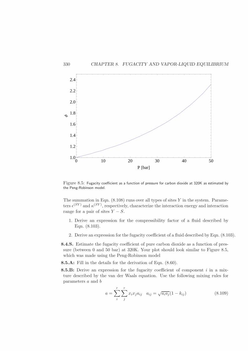
330 CHAPTER 8. FUGACITY AND VAPOR-LIQUID EQUILIBRIUM
0 10 20 30 40 501.0
1.2
1.4
1.6
1.8
2.0
2.2
2.4
P @barD
Φ
Figure 8.5: Fugacity coefficient as a function of pressure for carbon dioxide at 320K as estimated bythe Peng-Robinson model.
The summation in Eqn. (8.108) runs over all types of sites Y in the system. Parame-ters ǫ(SY ) and κ(SY ), respectively, characterize the interaction energy and interactionrange for a pair of sites Y − S.
1. Derive an expression for the compressibility factor of a fluid described byEqn. (8.103).
2. Derive an expression for the fugacity coefficient of a fluid described by Eqn. (8.103).
8.4.S. Estimate the fugacity coefficient of pure carbon dioxide as a function of pres-sure (between 0 and 50 bar) at 320K. Your plot should look similar to Figure 8.5,which was made using the Peng-Robinson model
8.5.A: Fill in the details for the derivation of Eqn. (8.60).
8.5.B: Derive an expression for the fugacity coefficient of component i in a mix-ture described by the van der Waals equation. Use the following mixing rules forparameters a and b
a =r∑
i
r∑
j
xixjaij aij =√aiaj(1− kij) (8.109)
331
and
b1/3 =
r∑
i
xib1/3i (8.110)
where kij is an adjustable parameter (a constant) which accounts for deviationsfrom a geometric-mean mixing rule.
8.5.C: Show that the fugacity coefficient of component i in a mixture described bythe Peng-Robinson equation of state is given by
log φi =bib(z−1)−log(z− bP
RT)− a
2√2bRT
(2∑
j yjaij
a− bib
)
log
(
v + b(1 +√2)
v + b(1−√2)
)
.
(8.111)Use Eqn. (8.109) as the mixing rule for parameter a, and Eqn. (7.88) for parameterb, where kij is an adjustable parameter (a constant) which accounts for deviationsfrom a geometric-mean mixing rule.
8.5.D: Show that the fugacity coefficient of component i in a mixture described bythe Redlich-Kwong equation of state is given by
log φi = logv
v − b+
biv − b
−2∑
j yjaji
RT 3/2blog
v + b
v+
abi
RT 3/2b2
(
logv + b
v
b
v + b
)
− log z. (8.112)
Use the same mixing rules as those suggested for the van der Waals fluid, Eqs. (7.87)and (7.88).
8.5.E: Show that, at low to intermediate pressures, the fugacity coefficient of com-ponent 1 in a binary mixture described by the van der Waals equation of state canbe expressed as
φ1 = exp
([
b1 −a1RT
] P
RT+
[√a1 −
√a2]
2y22P
(RT )2
)
. (8.113)
Use standard van der Waals mixing rules (Eqs. 7.87 and 7.88) for your derivation.(Hint: as a starting point, write the van der Waals equation in the approximateform Pv = RT + (b− a
RT )P + ..., and find an expression for v1).
8.5.F: Show that the fugacity coefficient of component i in a mixture of m compo-nents described by a virial equation of state is given by
log φi =2
v
r∑
j=1
yjBij +3
2v2
r∑
j=1
q∑
k=1
yjykCijk − log z. (8.114)
332 CHAPTER 8. FUGACITY AND VAPOR-LIQUID EQUILIBRIUM
8.5.G: Consider a binary mixture of two components. In the liquid phase, these twocomponents form a Lewis mixture. Assuming that, at low-to-moderate pressures,the vapor phase can be described by a virial equation truncated after the secondterm, could this mixture exhibit an azeotrope? Please explain.
8.5.H: Freeze-drying is often used in the food and pharmaceutical industries to re-move water from certain products. In this process, a solution of a given productis frozen, thereby yielding a solid material that contains a significant amount ofice crystals. The crystals are subsequently removed by sublimation. In order todesign an efficient process to remove these crystals, it is important to determine theconcentration of water in a carrier gas as a function of temperature. Ordinarily onewould use low pressures to eliminate ice, but in this particular instance you’re askedto consider the possibility of employing high-pressure nitrogen in an attempt to ar-rive at a more efficient drying process. In order to evaluate the feasibility of such aprocess, please determine the concentration of water in the gas phase at T = −10
and at P = 0.001, 0.1, 10, and 100 bar. Do you envisage any problems with theoperation of the process at 100 bar? Overall, would it be advantageous to conductthe process at 100 bar? You may assume that the vapor pressure of ice at −10Cis 1.956 torr, and that the specific volume of ice for the conditions relevant to thisproblem is approximately 1.09 cm3/gr. You may also assume that the product ofinterest is completely non-volatile.
8.5.I: A stream of moist air at 50 bar is to be cooled to -2C. What is the maximumamount of water that the gas phase can contain before water condenses? Pleaseconduct your calculations using (1) a virial equation truncated after the secondterm, and (2) a Redlich-Kwong equation. You may assume that air consists of abinary mixture of nitrogen (80%) and oxygen (20%). For this problem, you mayalso assume that the solubility of air in the water is small. How different are yourpredictions for the virial model and the Redlich-Kwong model?
8.5.J To perform bubble-point and dew-point calculations, it is useful to have aplot of T vs. x1 at fixed pressure, or P vs. x1 at fixed temperature for a binarymixture, with two curves.2 Using the van der Waals model with standard mixingrules, Eqs. (7.87) and (7.88), for benzene and toluene, make plots of T (at P = 1bar)and P (at T = 100C) vs. mole fraction benzene.
8.6.A: Derive Eqs.(8.73), (8.76), and (8.72).
8.6.B: Derive Eqn. (8.77).
8.6.C: The compressibility factor of a mixture of hard spheres of different diameters
2Examples of such curves are in §6.4 of [28].
333
can be determined from [?]:
zhs =6
πNAρ
(ζ0ζ31− ζ3
+3ζ1ζ2
(1− ζ3)2+
(3− ζ3)ζ23
(1− ζ3)3
)
(8.115)
where
ζk =πNAρ
6
r∑
i=1
xidik, (8.116)
and where ρ is the molar density, and di is the diameter of the molecules of speciesi. Use this expression to determine the molar volume (at constant pressure) of hard-sphere binary mixtures of different diameters, ranging from d1/d2 = 1 to d1/d2 = 5.Perform your calculations as a function of composition in the range x1 = 1 to x1 = 0.Use a pressure for your calculations such that the packing fraction of the spheres,given by η = (πNAρd
3)/6, is approximately η ≈ 0.3; for a system of hard spheresthis packing fraction corresponds to a liquid-like density. For which compositionsand diameter ratios does Amagat’s law provide a good description of the volume ofthe mixture?
8.6.C: Filling in the details of §8.6.3.1. Derive Raoult’s law for vapor-liquid equilibria in a multicomponent mixture.
State clearly all assumptions involved in your derivation.
2. Consider a binary mixture at constant pressure described by Raoult’s law. Isthe dew temperature curve a straight line? Is the bubble temperature curvea straight line? In both cases, please justify your answers.
8.6.D: Consider a binary mixture of components 1 and 2. Assume that both theliquid and the vapor form Lewis mixtures. Do not assume, however, that the vaporphase follows ideal-gas behavior.
1. Show that, in that case, Raoult’s law is not correct and should be replaced byan expression of the form
yiφpurei P = xiP
sati i = 1, 2 (8.117)
where φpurei is the fugacity coefficient of real gas i in the pure state. Stateclearly all assumptions involved in your derivation.
2. Show that, if the vapor phase can be described by a pressure-explicit virialequation truncated after the second term, the mole fraction in the vapor phaseis given by
yi =xiP
sati exp(
vi(P−P sati )
RT )
exp(BiPRT )(8.118)
334 CHAPTER 8. FUGACITY AND VAPOR-LIQUID EQUILIBRIUM
where Bi is the second virial coefficient of component i, and vi is the molarvolume of component i in the pure-liquid state.
8.7.A: Consider a stream of warm, moist air at 50 bar. This stream is to be usedfor air-conditioning purposes, and it is to be cooled to 20C. What is the maximumamount of water that the air can have before water starts condensing? You mayassume that air is a binary mixture of nitrogen (80%) and oxygen (20%). Pleaseconduct your calculations in the following two ways: 1) assume that the solubilityof nitrogen and oxygen in water can be neglected and, 2) take into account thesolubility of nitrogen and oxygen in water using Henry’s law. The Henry’s constants(in bar) for nitrogen and oxygen in water at 20C are logHN2−H2O = 4.8 andlogHO2−H2O = 4.55. The partial molar volumes of N2 and O2 in water at 25C andinfinite dilution are v∞N2
= 40 cm3/mol and v∞O2= 31 cm3/mol.
8.7.B: Predict the solubility of naphthelene in ethylene using a van der Waals modelwith the mixing rules used in Example 8.5.2.
The solubility of naphthalene in ethylene at T = 308.15K and P = 171 bar isapproximately ynaph = 0.01. The vapor pressure of naphthalene at this temperatureis P sat = 2.9 × 10⁻⁴ bar. The molar volume of solid naphthalene at this tempera-ture is v = 125 cm3/mol. What is the solubility at P = 30 bar and 308.15 K? Tosimplify your calculations, you may assume that the molar volume of the gas mix-ture is approximately equal to that of pure ethylene at the conditions of this problem.
species Tc (K) Pc (bar) Mw (g/mol)
naphthalene 748.4 40.5 128.2ethylene 282.4 50.4 28.05
[Hint: you may use critical property data to estimate parameters a and b, i.e.a = 27R2Tc
2/(64Pc) and b = RTc/(8Pc).]
8.7.C: Calculate the solubility of naphthalene in ethylene in the range P = [100 −300] bar and T = 285 − 325 K using the Peng-Robinson equation of state withk12 = 0.02. Compare your results to the experimental data of Tsekhanskaya et al.[?].
8.7.D: Moist air at 30 bar is cooled at constant pressure to −10C. What is themaximum permissible moisture content that the air may have to be sure that nomoisture condenses?
Assume that the volumetric properties of moist air at 30 bar are given by thevirial equation truncated after the second term. For this calculation, assume thatdry air is 80% nitrogen and 20% oxygen.
335
Data:
B33 = −1500 B12 = −15 (8.119)
B11 = −25 B13 = −63 (8.120)
B22 = −12 B23 = −72 (8.121)
where 1 stands for nitrogen, 2 for oxygen, and 3 for water. At −10C, the vaporpressure of ice is 1.95 torr, and the density of ice is 0.92 g/cm3. You may use thefollowing expression for the fugacity coefficient of component i in a multicomponentvirial gas
lnφi =P
RT
2m∑
j=1
xjBij −B
, (8.122)
where
B =m∑
i,j
xixjBij . (8.123)

336 CHAPTER 8. FUGACITY AND VAPOR-LIQUID EQUILIBRIUM
Chapter 9
Activity, Vapor-Liquid, andLiquid-Liquid Equilibrium
In Chapter 8, we discussed how to carry out phase equilibrium calculations by usingan arbitrary equation of state. The formalism presented in that chapter introducedthe concept of fugacity as a useful tool to conduct such calculations. Recall thatthe fugacity coefficient of component i in a mixture can be calculated by combiningEqs. (8.42) and (8.54)
log φi =
∫ P
0
zi − 1
PdP. (9.1)
The integral appearing in Eqn. (9.1) covers the range from 0 to pressure P ; themodel employed for zi must therefore be accurate over that whole range.
In recent years, much progress has been achieved in the development of accu-rate equation-of-state models for pure fluids and their mixtures. Some of the moresophisticated models are capable of describing the thermodynamic properties of flu-ids in both low and high density regimes. It is now possible to carry out integralssuch as that appearing in Eqn. (9.1) and arrive at reliable estimates of the fugacitycoefficient in mixtures, both vapor and liquid.
For many years, however, such models were not available; a parallel frameworkwas therefore developed for doing phase equilibrium calculations. In this framework,the fugacities and fugacity coefficients introduced in the previous chapter are usedfor the vapor phase, and another quantity was introduced for the liquid phase. Theliquid-, or condensed-phase framework is that of activity coefficients; in this chapterwe describe these and present some of the models that are traditionally used in thatcontext.
337
338 Chapter 9: Vapor-Liquid Equilibrium
9.1 Excess Properties and Activities
Recall that fugacities were more useful than chemical potential for two reasons.First, we did not need a fundamental relation—only a PV T equation of state.Secondly, we avoided the problems associated with going to zero pressure for anideal gas.
For estimating liquid fugacities we use activities, which have a structure analo-gous to fugacities themselves. For fugacities, we defined a residual property as thedifference between a real quantity and its ideal counterpart. Now we will introducean excess property as the difference between a real quantity and its Lewis mixingcounterpart. Before, we related fugacity to the exponential of the residual partialmolar Gibbs free energy. Now, we will relate activity to the exponential of a par-tial molar excess property. Finally, we introduce the activity coefficient in a wayanalogous to the fugacity coefficient.
Recall Lewis mixing behavior, presented in §8.6.1, which related the propertiesof mixtures to the properties of pure (real) species. We can then define excessproperties as a means to quantify the difference between an actual mixture propertyand that corresponding to a Lewis mixture. An excess property mE is thereforedefined by
ME(T, P, Ni) :=M(T, P, Ni)−MLewis(T, P, Ni). (9.2)
Just as we did for fugacity in a mixture, a partial molar excess property for compo-nent i is defined by
mEi (T, P, xi) := mi(T, P, xi)− mLewis
i (T, P, xi). (9.3)
And just as we did for partial molar residual properties, we could also define partialmolar excess properties as
mEi ≡
(∂ME
∂Ni
)
T,P,Nj 6=i
. (9.4)
From the properties of partial molar quantities, Eq. (8.14), we can also write
mE =
r∑
i=1
ximEi . (9.5)
Excess properties measure deviations from Lewis mixtures. For most systems, thosedeviations can be significant, particularly at intermediate to large concentrations. Itis instructive to consider experimental data for a few common solvents. Figure 9.1
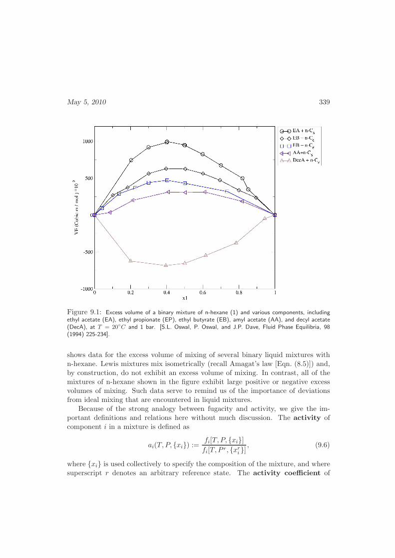
May 5, 2010 339
Figure 9.1: Excess volume of a binary mixture of n-hexane (1) and various components, includingethyl acetate (EA), ethyl propionate (EP), ethyl butyrate (EB), amyl acetate (AA), and decyl acetate(DecA), at T = 20C and 1 bar. [S.L. Oswal, P. Oswal, and J.P. Dave, Fluid Phase Equilibria, 98(1994) 225-234].
shows data for the excess volume of mixing of several binary liquid mixtures withn-hexane. Lewis mixtures mix isometrically (recall Amagat’s law [Eqn. (8.5)]) and,by construction, do not exhibit an excess volume of mixing. In contrast, all of themixtures of n-hexane shown in the figure exhibit large positive or negative excessvolumes of mixing. Such data serve to remind us of the importance of deviationsfrom ideal mixing that are encountered in liquid mixtures.
Because of the strong analogy between fugacity and activity, we give the im-portant definitions and relations here without much discussion. The activity ofcomponent i in a mixture is defined as
ai(T, P, xi) :=fi[T, P, xi]fi[T, P r, xri ]
, (9.6)
where xi is used collectively to specify the composition of the mixture, and wheresuperscript r denotes an arbitrary reference state. The activity coefficient of

340 Chapter 9: Vapor-Liquid Equilibrium
component i in the mixture is defined by
γi :=aixi, (9.7)
The excess partial molar Gibbs free energy of component i in the mixture can bewritten as
gEi := gi − gLewisi , (9.8)
or, after substitution of the fugacity, as
gEi := gi − gLewisi
= RT log
(fi
fLewisi
)
. (9.9)
If we now assume Lewis mixing, we have fLewisi = xif
purei , and Eqn. (9.9) becomes
gEi = RT log
(fi
xifpurei
)
. (9.10)
If we now set the fugacity fi[T, Pr, xri ] in Eqn. (9.6) to be that of the pure com-
ponent i, Eqn. (9.10) becomes
gEi = RT log γi. (9.11)
From the general properties of partial molar quantities, by multiplying each side ofEqn. (9.11) by xi and summing over all i, we also have
gE = RT∑
i
xi log γi. (9.12)
Note that, by construction, γi → 1 when xi → 1.
It can also be shown that the pressure dependence of an activity coefficient isrelated to the partial molar volume through an expression of the form
(∂ log γi∂P
)
T,x
=vEiRT
(9.13)
The temperature dependence is related to the partial molar enthalpy by an expres-sion of the form (
∂ log γi∂T
)
P,x
= − hEiRT 2
. (9.14)
May 5, 2010 341
9.2 Summary of Fugacity and Activity
At this point it is instructive to summarize and compare the approaches presentedfor the description of condensed-phase non-idealities and those presented earlier forvapor phases. Equilibrium conditions are found from equating temperature, pressureand fugacities. For vapor-liquid equilibrium, then, we write
fvapi = f liqi i = 1, . . . , r (9.15)
The vapor phase is written in terms of fugacity coefficients, and the liquid phase interms of activity coefficients
fvapi = f liqi i = 1, . . . , r
yiφvapi P = xiγif
purei i = 1, . . . , r (9.16)
where yi denotes the mole fraction of component i in the vapor phase, and xi denotesits mole fraction in the liquid phase. The fugacity coefficient is found by the relation
φi = exp
[gRiRT
]
= exp
[∫ P
0
zi − 1
PdP
]
. (9.1′)
Therefore, the fugacity coefficient can be found from a PV T equation of state forthe mixture in the gas phase.
On the liquid side, the activity coefficient is found from the excess property
γi = exp
[gEiRT
]
, (9.17)
which requires an equation of state for the excess property. To find the fugacity inthe pure state fpurei , we require a PV T equation of state for the pure component inthe vapor phase.
Table (9.1) provides an itemized comparison of the two approaches. As canbe seen from this table, the description outlined here in terms of activity coefficientclosely parallels the presentation in terms of fugacity coefficient; the only substantialdifference is that in the latter case the reference fluid was an ideal gas, whereas herethe reference fluid is a Lewis, or ideal mixture.
The remainder of this chapter discusses how to determine the activity coefficientγi in the liquid phase.
342 Chapter 9: Vapor-Liquid Equilibrium
Condensed Phase Vapor Phase
• measure deviations • measure deviationsfrom Lewis mixing from ideal-gas behavior
• excess properties: gE = g − gLewis • residual properties: gR = g − gideal gas
• activity coefficient: γi =fi
xifpurei
• fugacity coefficient: φi =fiyiP
• gEi = RT log γi • gRi = RT log φi
Table 9.1: Comparison of excess and residual properties.
9.3 Correlations for Partial Molar Excess Gibbs Free
Energy
9.3.1 Simple Binary Systems
For simplicity, we begin by discussing the case of a binary liquid mixture where thetwo components have similar size and chemistry. A general expression for the excessGibbs free energy of the mixture should be zero for the pure components. In theabsence of additional information, one can simply propose the following polynomialto describe excess molar Gibbs free energy data:
gE = Ax1x2, (9.18)
where A is a constant, which may depend on temperature and pressure, but notcomposition. Eqn. (9.18) is often referred to as a “two-suffix Margules equation”, oralso as a “one-parameter Margules equation”. This expression for gE leads to thefollowing equations for the activity coefficients:
RT log γ1 = Ax22
RT log γ2 = Ax21. (9.19)
Figure 9.2 shows experimental vapor-liquid equilibrium data for a binary mixtureof cycloheptane (1) and cyclopentanol (2) at 25C. The line is a fit to the data usinga two-suffix Margules equation and assuming that the vapor phase is an ideal gas.Figure 9.3 shows the corresponding activity coefficients for this mixture, and FigureWhere are these
plots from? Do weneed permission?JDS 07/13/2007
9.3 the excess molar Gibbs free energy. The excess Gibbs free energy data are fairlysymmetric and can be described by a two-suffix Margules equation.
Example 9.3.1 Use the Margules model to predict the boiling point and vapor com-position for a mixture of cycloheptane (species 1) and cyclopentanol (species 2) ofarbitrary composition. Assume atmospheric pressure, Patm = 1.01325bar, and thevalue A = 4.06kJ, estimated by Brown and Smith [?].
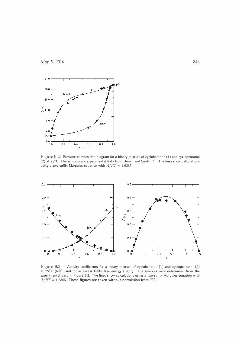
May 5, 2010 343
Figure 9.2: Pressure-composition diagram for a binary mixture of cycloheptane (1) and cyclopentanol(2) at 25C. The symbols are experimental data from Brown and Smith [?]. The lines show calculationsusing a two-suffix Margules equation with A/RT = 1.6385.
Figure 9.3: Activity coefficients for a binary mixture of cycloheptane (1) and cyclopentanol (2)at 25C (left), and molar excess Gibbs free energy (right). The symbols were determined from theexperimental data in Figure 9.2. The lines show calculations using a two-suffix Margules equation withA/RT = 1.6385. These figures are taken without permission from ???
344 Chapter 9: Vapor-Liquid Equilibrium
Solution: The fugacities of each component must be the same in both phases
f li = fv
i , i = 1, 2
xiγlif
purei = yiφ
vi P, i = 1, 2, (9.20)
where yi is used to denote the composition of the vapor phase and xi that ofthe liquid. Superscripts v and l denote a quantity evaluated at the vapor orliquid phase composition, respectively. As is customary, we write the liquidphase in terms of activity coefficients and the vapor phase in terms of fugacitycoefficients. We do this because the liquid phase is dominated by energetics ofinteractions between the molecules, whereas the vapor phase is dominated bythe entropy, and, therefore, pressure. To first approximation, we neglect non-ideality in the vapor phase. We also use the approximation for the pure, liquidfugacity derived earlier, Eqn. (8.50). Therefore, our equal-fugacity equationsbecome
xiγliP
sati exp
[∫ Patm
P sati
vpurei (T, P ′)
RTdP ′
]
∼= yiPatm, i = 1, 2. (9.21)
At atmospheric pressure, it is safe to neglect the Poynting correction factor fora liquid
xiγliP
sati = yiPatm, i = 1, 2.
xi exp
[A(1 − xi)
2
RT
]
P sati = yiPatm, i = 1, 2, (9.22)
where we have inserted the Margules estimate for the activity coefficient. Wecan estimate the saturation pressures for cycloheptane using the Antoine Equa-tion, (4.49). The parameters are found from Poling, Prausnitz and O’Connell[70] to be A1 = 3.96330, B1 = 1322.22, and C1 = −57.853. The saturationpressure for cyclopentanol uses a generalized form
log
(Psat
Pc
)
=
(TcT
)[
a2
(
1− T
Tc
)
+ b2
(
1− T
Tc
)3/2
+
c2
(
1− T
Tc
)5/2
+ d2
(
1− T
Tc
)5]
, (9.23)
where Tc = 619.5K, a2 = −7.40984, b2 = 1.71852, c2 = −6.8471, and d2 =−4.36177. We can eliminate two of the variables, since x2 = 1 − x1, andy2 = 1− y1. We currently have two unknowns, T and y1. We can eliminate thelatter by summing each side of Eqn. (9.22) for the two components to obtain
x1 exp
[A(x1)
2
RT
]
P sat1 [T ] + (1 − x1) exp
[A(1− x1)
2
RT
]
P sat2 [T ] = Patm.
(9.24)
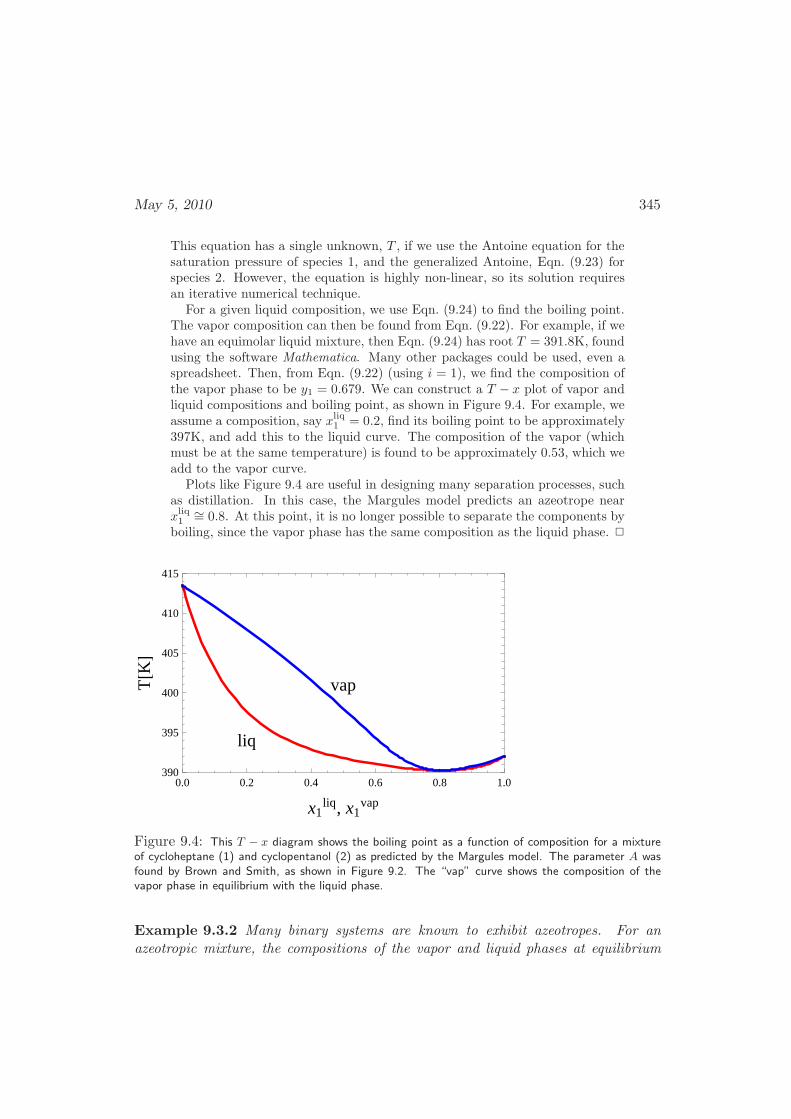
May 5, 2010 345
This equation has a single unknown, T , if we use the Antoine equation for thesaturation pressure of species 1, and the generalized Antoine, Eqn. (9.23) forspecies 2. However, the equation is highly non-linear, so its solution requiresan iterative numerical technique.
For a given liquid composition, we use Eqn. (9.24) to find the boiling point.The vapor composition can then be found from Eqn. (9.22). For example, if wehave an equimolar liquid mixture, then Eqn. (9.24) has root T = 391.8K, foundusing the software Mathematica. Many other packages could be used, even aspreadsheet. Then, from Eqn. (9.22) (using i = 1), we find the composition ofthe vapor phase to be y1 = 0.679. We can construct a T − x plot of vapor andliquid compositions and boiling point, as shown in Figure 9.4. For example, weassume a composition, say xliq1 = 0.2, find its boiling point to be approximately397K, and add this to the liquid curve. The composition of the vapor (whichmust be at the same temperature) is found to be approximately 0.53, which weadd to the vapor curve.
Plots like Figure 9.4 are useful in designing many separation processes, suchas distillation. In this case, the Margules model predicts an azeotrope nearxliq1
∼= 0.8. At this point, it is no longer possible to separate the components byboiling, since the vapor phase has the same composition as the liquid phase. 2
liq
vap
0.0 0.2 0.4 0.6 0.8 1.0390
395
400
405
410
415
x1liq, x1
vap
T@KD
Figure 9.4: This T − x diagram shows the boiling point as a function of composition for a mixtureof cycloheptane (1) and cyclopentanol (2) as predicted by the Margules model. The parameter A wasfound by Brown and Smith, as shown in Figure 9.2. The “vap” curve shows the composition of thevapor phase in equilibrium with the liquid phase.
Example 9.3.2 Many binary systems are known to exhibit azeotropes. For anazeotropic mixture, the compositions of the vapor and liquid phases at equilibrium
346 Chapter 9: Vapor-Liquid Equilibrium
are identical, as shown in the previous example. Lewis mixtures cannot give rise toazeotropic behavior; in order to describe azeotropic mixtures, it is necessary to takeinto account departures from Lewis mixing in the liquid phase.
A classic azeotropic mixture is provided by ethanol (1) and water (2). Theazeotropic composition is approximately x1 = 0.89. The boiling temperature of thatmixture is approximately 79C. The vapor pressures of ethanol and water can bedetermined from the following Antoine-type equations1
log10 Psat1 (kPa) = 16.6758 − 3674.49
T (C) + 226.45
log10 Psat2 (kPa) = 16.262 − 3799.89
T (C) + 226.35.
(9.25)
Use this information to estimate constant A for a one-parameter Margules equation.
Solution: For phase equilibrium between a liquid and a vapor, we write
fvapi = f liq
i , i = 1, 2
yiφvapi P = xiγif
purei , i = 1, 2. (9.26)
For simplicity, we assume that the vapor phase is an ideal gas. For an azeotropicmixture, x1 = y1; Eqns.(9.26) therefore reduce to
P = P sat1 γ1 = P sat
2 γ2, (9.27)
when we neglect the Poynting correction factor. If a one-parameter Margulesequation is employed, we have
A
RT=
1
x22 − x21log
P sat2
P sat1
. (9.28)
At T = 79C, we getA
RT= 1.062. (9.29)
It is important to point out that in this example we use a simple one-parameterMargules equation to describe non-ideality in the ethanol-water mixture. Thismixture, however, is highly non-ideal and more elaborate models are necessaryto describe it over wide ranges of composition, temperature, and pressure. 2
In the limit of infinite dilution, i.e. in the limit when the concentration ofone of the components approaches zero, the activity coefficients of a one-parameter
1See Eqn. (4.49), and Table D.4 for more details.
May 5, 2010 347
Margules equation tend to
γ∞1 = exp
(A
RT
)
γ∞2 = exp
(A
RT
)
, (9.30)
which shows one of the shortcomings of the Margules model: the infinite-dilutionactivity coefficients of components 1 and 2 are identical, regardless of their chemicalidentity. This is generally not the case, and to avoid this oversimplification it isnecessary to resort to a more “flexible” expression containing more adjustable pa-rameters. More generally, the excess molar Gibbs free energy can, for example, beexpanded in the order parameter x1 − x2 to give
gE = x1x2[A+B(x1 − x2) + C(x1 − x2)
2 + . . .], (9.31)
where the number of terms in the series depends on the asymmetry and the qualityof the data to be correlated with that expression. Equation (9.31) is known as theRedlich-Kister expansion.
9.3.2 Thermodynamic Consistency
As indicated by Eqn. (9.11), the logarithm of an activity coefficient is a partial molarproperty. As such, it obeys a relationship of the form
∑
i
xid log γi = 0 constant T and P. (9.32)
In other words, the activity coefficients of the various components that constitutea mixture are not independent of each other. In a binary system, Eqn. (9.32)implies that it is possible to determine the activity coefficient of one componentfrom knowledge of the other. Alternatively, Eqn. (9.32) can also be used to test theconsistency between experimental phase equilibrium data for a binary mixture. Thefollowing example serves to illustrate these ideas.
Example 9.3.3 Let us assume that experimental data for the activity coefficient ofcomponent 1 in a binary mixture can be correlated by a simple polynomial of theform:
log γ1 = a1x22 + a2x
32 + a3x
42, (9.33)
where the ai are adjustable parameters. What general form should the correlationfor log γ2 follow in order to be consistent with Eqn. (9.33) ?
348 Chapter 9: Vapor-Liquid Equilibrium
Solution: From Eqn. (9.32), we can write
d log(γ1/γ2)
dx2=
1
x2
d log γ1dx2
, (9.34)
which, after substitution of Eqn. (9.33), gives
d log(γ1/γ2)
dx2= 2a1 + 3a2x2 + 4a3x
22. (9.35)
Integration of that expression results in
log γ2 = log γ1 −(
2a1x2 +3
2a2x
22 +
4
3a3x
32
)
+ C, (9.36)
where C is a constant of integration. To evaluate it, we recall that for x2 = 1we should recover γ2 = 1; the result for C is
C = a1 +1
2a2 +
1
3a3. (9.37)
The final expression for log γ2 is therefore given by
log γ2 =
(
a1 +3
2a2 + 2a3
)
x21 −(
a2 +8
3a3
)
x31 + a3x41. (9.38)
2
Example 9.3.4 Let us assume that experimental data are available for the activitycoefficients of both components of a binary mixture. Show that
∫ 1
0log
(γ1γ2
)
dx1 = 0. (9.39)
Solution: From the general properties of partial molar quantities we canwrite
gE
RT= x1 log γ1 + x2 log γ2. (9.40)
After differentiation with respect to x1 we have
d(gE/RT )
dx1= x1
∂ log γ1∂x1
+ log γ1 + x2∂ log γ2∂x1
+ log γ2dx2dx1
, (9.41)
which, given that dx1 = −dx2, can also be written as
d(gE/RT )
dx1= log
(γ1γ2
)
. (9.42)
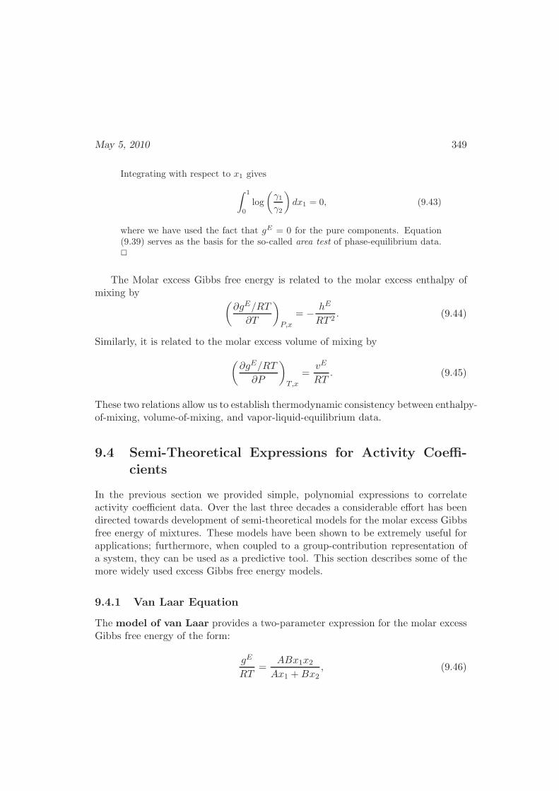
May 5, 2010 349
Integrating with respect to x1 gives
∫ 1
0
log
(γ1γ2
)
dx1 = 0, (9.43)
where we have used the fact that gE = 0 for the pure components. Equation(9.39) serves as the basis for the so-called area test of phase-equilibrium data.2
The Molar excess Gibbs free energy is related to the molar excess enthalpy ofmixing by
(∂gE/RT
∂T
)
P,x
= − hE
RT 2. (9.44)
Similarly, it is related to the molar excess volume of mixing by
(∂gE/RT
∂P
)
T,x
=vE
RT. (9.45)
These two relations allow us to establish thermodynamic consistency between enthalpy-of-mixing, volume-of-mixing, and vapor-liquid-equilibrium data.
9.4 Semi-Theoretical Expressions for Activity Coeffi-cients
In the previous section we provided simple, polynomial expressions to correlateactivity coefficient data. Over the last three decades a considerable effort has beendirected towards development of semi-theoretical models for the molar excess Gibbsfree energy of mixtures. These models have been shown to be extremely useful forapplications; furthermore, when coupled to a group-contribution representation ofa system, they can be used as a predictive tool. This section describes some of themore widely used excess Gibbs free energy models.
9.4.1 Van Laar Equation
The model of van Laar provides a two-parameter expression for the molar excessGibbs free energy of the form:
gE
RT=
ABx1x2Ax1 +Bx2
, (9.46)
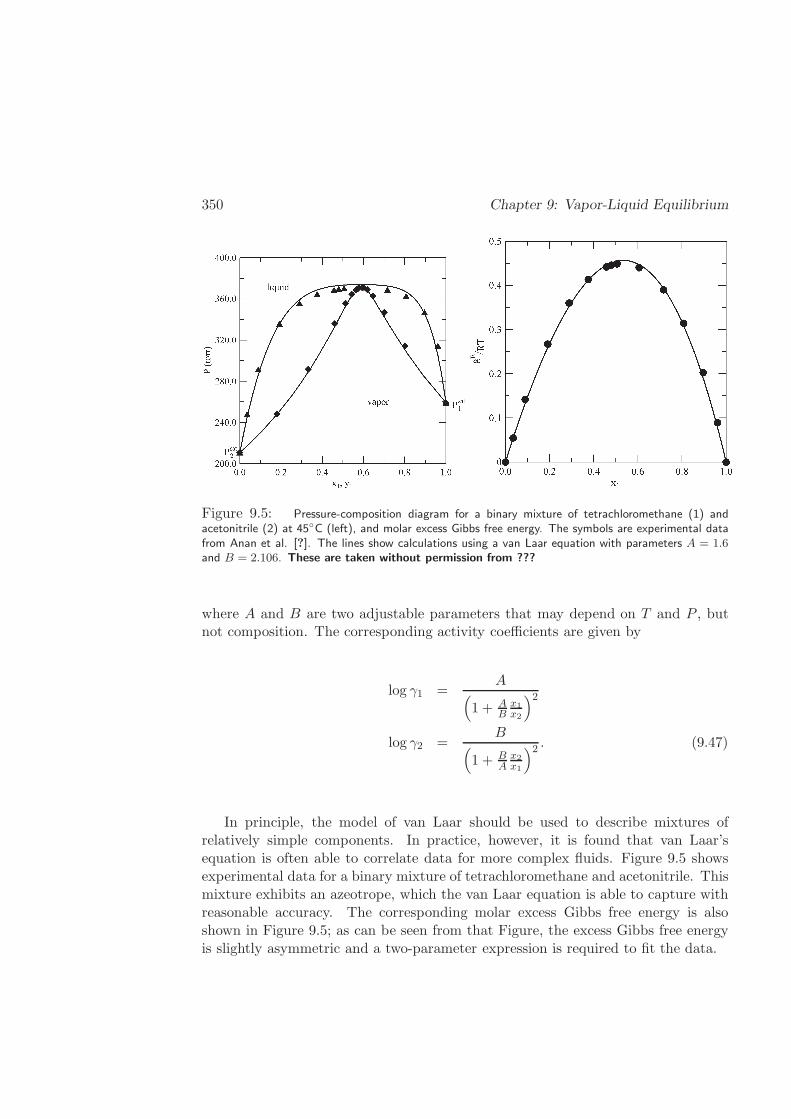
350 Chapter 9: Vapor-Liquid Equilibrium
Figure 9.5: Pressure-composition diagram for a binary mixture of tetrachloromethane (1) andacetonitrile (2) at 45C (left), and molar excess Gibbs free energy. The symbols are experimental datafrom Anan et al. [?]. The lines show calculations using a van Laar equation with parameters A = 1.6and B = 2.106. These are taken without permission from ???
where A and B are two adjustable parameters that may depend on T and P , butnot composition. The corresponding activity coefficients are given by
log γ1 =A
(
1 + ABx1x2
)2
log γ2 =B
(
1 + BAx2x1
)2 . (9.47)
In principle, the model of van Laar should be used to describe mixtures ofrelatively simple components. In practice, however, it is found that van Laar’sequation is often able to correlate data for more complex fluids. Figure 9.5 showsexperimental data for a binary mixture of tetrachloromethane and acetonitrile. Thismixture exhibits an azeotrope, which the van Laar equation is able to capture withreasonable accuracy. The corresponding molar excess Gibbs free energy is alsoshown in Figure 9.5; as can be seen from that Figure, the excess Gibbs free energyis slightly asymmetric and a two-parameter expression is required to fit the data.
May 5, 2010 351
9.4.2 Wilson’s Equation
In Wilson’s equation, the molar excess Gibbs free energy is given by
gE
RT= −x1 log(x1 + Λ12x2)− x2 log(x2 + Λ21x1), (9.48)
where Λ21 and Λ12 are two adjustable parameters. These parameters are assumedto depend on temperature according to
Λ12 =v2v1
exp
[
−λ12 − λ11RT
]
(9.49)
Λ21 =v1v2
exp
[
−λ12 − λ22RT
]
, (9.50)
where vi represents the molar volume of pure component i, and where λij − λiirepresents a difference between the interaction energy of ij versus ii pairs. Thesedifferences are not too sensitive to temperature, and are often assumed to be con-stant. Note, however, that in practice, parameters Λ21 and Λ12 are determineddirectly by regression of experimental data, and little regard is given to the func-tional form suggested by Eqns.(9.49) and (9.50).
It can be shown that the activity coefficients derived from Wilson’s excess Gibbsfree energy model are given by
log γ1 = − log(x1 + Λ12x2) + x2
[Λ12
x1 + Λ12x2− Λ21
x2 + Λ21x1
]
(9.51)
log γ2 = − log(x2 + Λ21x1)− x1
[Λ12
x1 + Λ12x2− Λ21
x2 + Λ21x1
]
. (9.52)
9.4.3 NRTL Equation
The NRTL equation is often used to describe the activity coefficients of highly non-ideal mixtures. In this model, the excess Gibbs free energy is given by:
gE
RT= x1x2
(τ21G21
x1 + x2G21+
τ12G12
x2 + x1G12
)
, (9.53)
where τ21 and τ12 are two adjustable parameters, whose physical significance isloosely related to energy parameters characteristic of the 1-1, 2-2, and 1-2 interac-tions. The Gij parameters are related to the τij through
G12 = exp(
−α τ12RT
)
, G21 = exp(
−α τ21RT
)
, (9.54)
352 Chapter 9: Vapor-Liquid Equilibrium
where α is also an adjustable parameter, usually set to a value of 0.2. The activitycoefficients corresponding to Eqn. (9.53) are
log γ1 = x22
[
τ21
(G21
x1 + x2G21
)2
+τ12G12
(x2 + x1G12)2
]
,
log γ2 = x21
[
τ12
(G12
x2 + x1G12
)2
+τ21G21
(x1 + x2G21)2
]
. (9.55)
9.4.4 UNIQUAC Model
In the UNIQUAC model, the molar excess Gibbs free energy is written as the sumof combinatorial contributions, arising from entropic contributions, and residualcontributions, mostly due to intermolecular forces. Since the combinatorial part ofthe free energy is entropic in nature, it depends only on composition and on pure-component data. The residual part, however, includes two adjustable parameterswhich are meant to consider intermolecular interactions.
The molar excess Gibbs free energy is given by
gE
RT=
(gE
RT
)
combinatorial
+
(gE
RT
)
residual
, (9.56)
where, for a binary mixture,
(gE
RT
)
combinatorial
= x1 logΦ1
x1+ x2 log
Φ2
x2+zl2
(
x1q1 logθ1Φ1
+ x2q2 logθ2Φ2
)
(gE
RT
)
residual
= −x1q′1 log(θ′1 + θ′2τ21)− x2q′2 log(θ
′2 + θ′1τ12), (9.57)
where zl has the meaning of a coordination number, usually set to 10. ParameterΦ has the meaning of a segment fraction, and θ and θ′ have the meaning of area
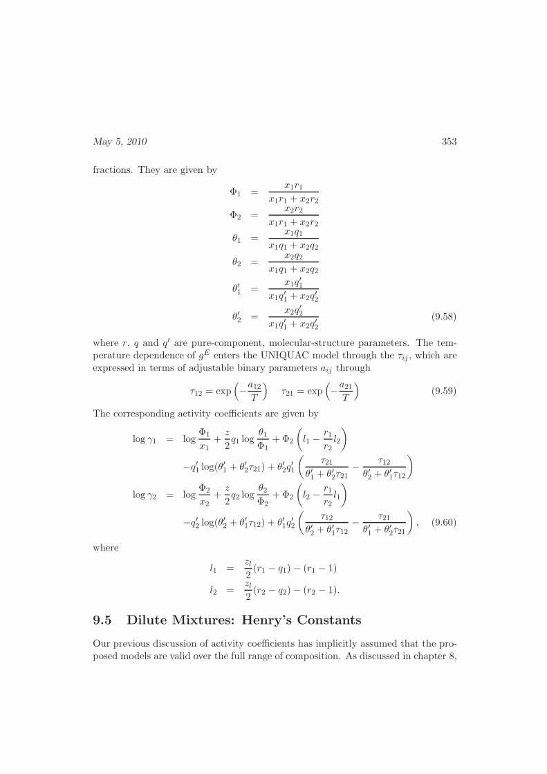
May 5, 2010 353
fractions. They are given by
Φ1 =x1r1
x1r1 + x2r2
Φ2 =x2r2
x1r1 + x2r2
θ1 =x1q1
x1q1 + x2q2
θ2 =x2q2
x1q1 + x2q2
θ′1 =x1q
′1
x1q′1 + x2q
′2
θ′2 =x2q
′2
x1q′1 + x2q
′2
(9.58)
where r, q and q′ are pure-component, molecular-structure parameters. The tem-perature dependence of gE enters the UNIQUAC model through the τij , which areexpressed in terms of adjustable binary parameters aij through
τ12 = exp(
−a12T
)
τ21 = exp(
−a21T
)
(9.59)
The corresponding activity coefficients are given by
log γ1 = logΦ1
x1+z
2q1 log
θ1Φ1
+Φ2
(
l1 −r1r2l2
)
−q′1 log(θ′1 + θ′2τ21) + θ′2q′1
(τ21
θ′1 + θ′2τ21− τ12θ′2 + θ′1τ12
)
log γ2 = logΦ2
x2+z
2q2 log
θ2Φ2
+Φ2
(
l2 −r1r2l1
)
−q′2 log(θ′2 + θ′1τ12) + θ′1q′2
(τ12
θ′2 + θ′1τ12− τ21θ′1 + θ′2τ21
)
, (9.60)
where
l1 =zl2(r1 − q1)− (r1 − 1)
l2 =zl2(r2 − q2)− (r2 − 1).
9.5 Dilute Mixtures: Henry’s Constants
Our previous discussion of activity coefficients has implicitly assumed that the pro-posed models are valid over the full range of composition. As discussed in chapter 8,
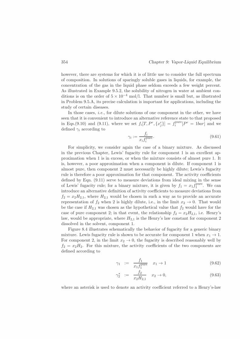
354 Chapter 9: Vapor-Liquid Equilibrium
however, there are systems for which it is of little use to consider the full spectrumof composition. In solutions of sparingly soluble gases in liquids, for example, theconcentration of the gas in the liquid phase seldom exceeds a few weight percent.As illustrated in Example 9.5.2, the solubility of nitrogen in water at ambient con-ditions is on the order of 5 × 10⁻⁴ mol/l. That number is small but, as illustratedin Problem 9.5.A, its precise calculation is important for applications, including thestudy of certain diseases.
In those cases, i.e., for dilute solutions of one component in the other, we haveseen that it is convenient to introduce an alternative reference state to that proposedin Eqs.(9.10) and (9.11), where we set fi[T, P
r, xrj] = fpurei [P r = 1bar] and wedefined γi according to
γi :=fi
xifpurei
. (9.61)
For simplicity, we consider again the case of a binary mixture. As discussedin the previous Chapter, Lewis’ fugacity rule for component 1 is an excellent ap-proximation when 1 is in excess, or when the mixture consists of almost pure 1. Itis, however, a poor approximation when a component is dilute. If component 1 isalmost pure, then component 2 must necessarily be highly dilute; Lewis’s fugacityrule is therefore a poor approximation for that component. The activity coefficientsdefined by Eqn. (9.11) serve to measure deviations from ideal mixing in the senseof Lewis’ fugacity rule; for a binary mixture, it is given by f1 = x1f
pure1 . We can
introduce an alternative definition of activity coefficients to measure deviations fromf2 = x2H2,1, where H2,1 would be chosen in such a way as to provide an accuraterepresentation of f2 when 2 is highly dilute, i.e., in the limit x2 → 0. That wouldbe the case if H2,1 was chosen as the hypothetical value that f2 would have for thecase of pure component 2; in that event, the relationship f2 = x2H2,1, i.e. Henry’slaw, would be appropriate, where H2,1 is the Henry’s law constant for component 2dissolved in the solvent, component 1.
Figure 8.4 illustrates schematically the behavior of fugacity for a generic binarymixture. Lewis fugacity rule is shown to be accurate for component 1 when x1 → 1.For component 2, in the limit x2 → 0, the fugacity is described reasonably well byf2 = x2H2. For this mixture, the activity coefficients of the two components aredefined according to
γ1 :=f1
x1fpure1
x1 → 1 (9.62)
γ∗2 :=f2
x2H2,1x2 → 0, (9.63)
where an asterisk is used to denote an activity coefficient referred to a Henry’s-law
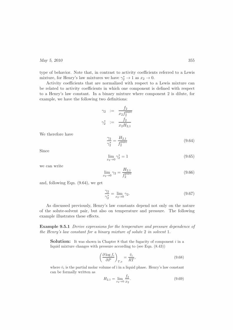
May 5, 2010 355
type of behavior. Note that, in contrast to activity coefficients referred to a Lewismixture, for Henry’s law mixtures we have γ∗2 → 1 as x2 → 0.
Activity coefficients that are normalized with respect to a Lewis mixture canbe related to activity coefficients in which one component is defined with respectto a Henry’s law constant. In a binary mixture where component 2 is dilute, forexample, we have the following two definitions:
γ2 :=f2
x2fpure2
γ∗2 :=f2
x2H2,1
We therefore haveγ2γ∗2
=H2,1
fpure2
(9.64)
Since
limx2→0
γ∗2 = 1 (9.65)
we can write
limx2→0
γ2 =H2,1
fpure2
(9.66)
and, following Eqn. (9.64), we get
γ2γ∗2
= limx2→0
γ2. (9.67)
As discussed previously, Henry’s law constants depend not only on the natureof the solute-solvent pair, but also on temperature and pressure. The followingexample illustrates these effects.
Example 9.5.1 Derive expressions for the temperature and pressure dependence ofthe Henry’s law constant for a binary mixture of solute 2 in solvent 1.
Solution: It was shown in Chapter 8 that the fugacity of component i in aliquid mixture changes with pressure according to (see Eqn. (8.43))
(∂ log fi∂P
)
T,x
=viRT
, (9.68)
where vi is the partial molar volume of i in a liquid phase. Henry’s law constantcan be formally written as
H2,1 = limx2→0
f2x2. (9.69)
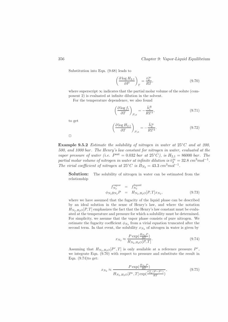
356 Chapter 9: Vapor-Liquid Equilibrium
Substitution into Eqn. (9.68) leads to(∂ logH2,1
∂P
)
T
=v∞2RT
, (9.70)
where superscript ∞ indicates that the partial molar volume of the solute (com-ponent 2) is evaluated at infinite dilution in the solvent.
For the temperature dependence, we also found
(∂ log fi∂T
)
P,x
= − hRiRT 2
, (9.71)
to get(∂ logH2,1
∂T
)
P,x
= − h∞2RT 2
. (9.72)
2
Example 9.5.2 Estimate the solubility of nitrogen in water at 25C and at 200,500, and 1000 bar. The Henry’s law constant for nitrogen in water, evaluated at thevapor pressure of water (i.e. P sat = 0.032 bar at 25C), is H2,1 = 86000 bar. Thepartial molar volume of nitrogen in water at infinite dilution is v∞2 = 32.8 cm3mol−1.The virial coefficient of nitrogen at 25C is BN2 = 43.3 cm3mol−1.
Solution: The solubility of nitrogen in water can be estimated from therelationship
fvaporN2
= f liquidN2
φN2yN2P = HN2,H2O[P, T ]xN2 , (9.73)
where we have assumed that the fugacity of the liquid phase can be describedby an ideal solution in the sense of Henry’s law, and where the notationHN2,H2O[P, T ] emphasizes the fact that the Henry’s law constant must be evalu-ated at the temperature and pressure for which a solubility must be determined.For simplicity, we assume that the vapor phase consists of pure nitrogen. Weestimate the fugacity coefficient φN2 from a virial equation truncated after thesecond term. In that event, the solubility xN2 of nitrogen in water is given by
xN2 ≈ P exp(BN2P
RT )
HN2,H2O[P, T ]. (9.74)
Assuming that HN2,H2O[Pr, T ] is only available at a reference pressure P r,
we integrate Eqn. (9.70) with respect to pressure and substitute the result inEqn. (9.74)to get:
xN2 ≈ P exp(BN2P
RT )
HN2,H2O[Pr, T ] exp(
v∞N2
(P−P r)
RT ), (9.75)
May 5, 2010 357
where we have approximated the partial molar volume of nitrogen at infinitedilution v∞N2
to be independent of P . Since BN2 , HN2,H2O[Psat, T ] and v∞N2
are all available at 25C, this equation can now be used to estimate nitrogensolubilities in water over a range of pressures (at that temperature).
By assuming that the liquid phase is an ideal solution in the sense of Henry’slaw, we implicitly assumed that the activity coefficient of the nitrogen in theliquid phase is unity. At high enough pressures, however, the concentrationof nitrogen in the liquid can become sufficiently high to introduce appreciabledeviations from ideal mixing. In that event, liquid-phase non-idealities shouldbe taken into account, i.e.
f liqN2
= xN2γ∗N2HN2,H2O, (9.76)
where, as mentioned above, the asterisk serves to remind us that the activitycoefficient for nitrogen is normalized with respect to a Henry’s law frame ofreference. For the purposes of this example, a simple activity coefficient modelsuffices; we use a one-suffix Margules equation What exactly is the
difference between aone- and a two-suffixMargules equation?Below the samemodel seems to becalled two-suffix.JDS 07/13/2007.
log γH2O =A
RTx2N2
. (9.77)
For nitrogen, following Eqn. (9.67), we have
log γ∗N2=
A
RT(x2H2O − 1) . (9.78)
The fugacity of nitrogen in the liquid can therefore be written as
logf liqN2
xN2
= logHN2,H2O[PsatH2O, T ] +
A
RT(x2H2O − 1) +
v∞N2(P − P sat
H2O)
RT. (9.79)
Eqn. (9.79) can now be used to estimate the fugacity of nitrogen in water, andthe compositions of the vapor and liquid phases can be estimated from:
φN2yN2P = xN2HN2,H2O[PsatH2O, T ] exp
(A
RTx2N2
+v∞N2
(P − P satH2O
)
RT
)
φH2OyH2OP = xH2OγH2OPsatH2O. (9.80)
2
9.5.1 Measurement of Activity Coefficients
Freezing Point Depression
Upon addition of a solute to a liquid, the freezing point of the newly formed solutiondecreases. This can be explained using stability arguments. It is possible to showthat this is a general feature, and works for any solute in the liquid. Our proof

358 Chapter 9: Vapor-Liquid Equilibrium
begins with a figure similar to Figure 4.7. In that figure, the saturation pressure iswhere the chemical potentials of the two phases intersect. To look at freezing pointdepression now we plot the chemical potential vs. temperature, for a solid and liquid.Such a sketch is made in Figure 9.6. First, we can show that the liquid line is alwayssteeper than the solid line. The slope of each line on this plot is the derivative
(∂µ
∂T
)
P
=
(∂g
∂T
)
P
= −s. (9.81)
Since the entropy of the liquid is always greater than that of the solid, it must havea steeper slope on this plot, and the sketch must have this general form. Note thatthe melting temperature of the solvent is the intersection of these two curves, T pure
melt ,as shown in the figure. Now we add solute to the solvent. The chemical potentialof the solid remains unchanged, since the solute enters only the liquid. We can findthe direction that the liquid line moves on this plot. Actually, it is easier to considerhow the liquid line moves as we add more solvent (species 1), diluting the solute(species 2)
(∂µ1∂N1
)
T,P,N2
=
(∂2G
∂N21
)
T,P,N2
> 0, (9.82)
which follows from the definition of the chemical potential, and the stability ar-guments of §4.1. Recall from that section that stability requires all second orderderivatives with respect to extensive independent variables of any potential to bepositive. Since G is a potential and N1 is extensive, the derivative must be positiveas shown. In words, this relation shows that chemical potential of solvent must in-crease with increasing solvent, which means it must decrease with increasing solute.Therefore, the chemical potential of the solute/solvent mixture must lie below theline for the pure solvent, as shown in Figure 9.6. The new melting point is wherethe chemical potential of the solvent intersects with the chemical potential of thepure solid. As shown, this new melting point, Tmix
melt must be lower than the puremelting point. Note that we made no assumptions to derive this result, which mustbe general.
The so-called freezing point depression can be used to measure the activity co-efficient of the solvent in such a dilute mixture. If subscript (1) is used to denotethe solvent, the chemical potential of the solvent in the mixture can be written as
µ1[T, P ] = µpure liquid1 [T, P ] +RT log a1, (9.83)
where a1 is the activity. If the solid phase in equilibrium with the solution is assumedto be pure, at the melting point of the solution, T ′, we have
µ1[T′, P ] = µpure solid
1 [T ′, P ]. (9.84)
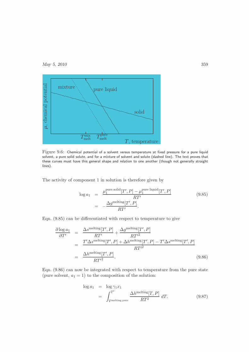
May 5, 2010 359
mixture
solid
pure liquid
T , temperature
µ,ch
emic
alpot
enti
al
TpuremeltTmix
melt
Figure 9.6: Chemical potential of a solvent versus temperature at fixed pressure for a pure liquidsolvent, a pure solid solute, and for a mixture of solvent and solute (dashed line). The text proves thatthese curves must have this general shape and relation to one another (though not generally straightlines).
The activity of component 1 in solution is therefore given by
log a1 =µpure solid1 [T ′, P ]− µpure liquid
1 [T ′, P ]RT ′ (9.85)
= −∆gmelting[T ′, P ]RT ′ .
Eqn. (9.85) can be differentiated with respect to temperature to give
∂ log a1∂T ′ =
∆smelting[T ′, P ]RT ′ +
∆gmelting[T ′, P ]
RT ′2
=T ′∆smelting[T ′, P ] + ∆hmelting[T ′, P ]− T ′∆smelting[T ′, P ]
RT ′2
=∆hmelting[T ′, P ]
RT ′2 . (9.86)
Eqn. (9.86) can now be integrated with respect to temperature from the pure state(pure solvent, a1 = 1) to the composition of the solution:
log a1 = log γ1x1
=
∫ T ′
Tmelting,pure
∆hmelting[T, P ]
RT 2dT. (9.87)
360 Chapter 9: Vapor-Liquid Equilibrium
For small concentrations of the solute (component 2) the logarithm in Eqn. (9.87)can be expanded in a series. If a two-suffix Margules equation is used for the activitycoefficient, we get
log γ1x1 = log γ1 − x2 −1
2x22 + ...
= (A− 1
2)x22 − x2. (9.88)
Furthermore, for small concentrations of the solute the freezing point depression islikely to be small; in that case we can expect ∆hmelting,pure to be approximately con-stant in the interval Tmelting,pure−T ′, and Eqs. (9.87) and 9.88 to be approximatelyequivalent to
A =1
2+
1
x22
[
x2 +∆hmelting,pure
1
R
(1
Tmelting,pure− 1
T ′
)]
, (9.89)
which provides a means for estimating constant A from knowledge of the enthalpychange of melting, the concentration, and the freezing-point depression experiencedfor that concentration.
Osmotic Pressure
For solutions of macromolecules (e.g., polymers or proteins), osmotic pressure mea-surements provide a convenient means for estimating activity coefficients. In thesemeasurements, a macromolecule solution is separated from a solvent reservoir bya semi-permeable membrane. See Figure 9.7. The pressure on the macromolecule-solution side rises above that on the solvent-reservoir side by an amount Π[x2, T ],i.e., the osmotic pressure of the solution at concentration x2 of the solute.
At equilibrium, the chemical potential of the solvent on both sides of the mem-brane must be the same. We therefore can write for the solvent
fpure1 [P, T ] = f1[x1, P +Π, T ], (9.90)
or
fpure1 [P +Π, T ] = x1γ1[x1, P +Π, T ]fpure1 [P +Π, T ]. (9.91)
Since
log
(fpure1 [P +Π, T ]
fpure1 [P, T ]
)
=
∫ P+Π
P
v1RT
dP, (9.92)
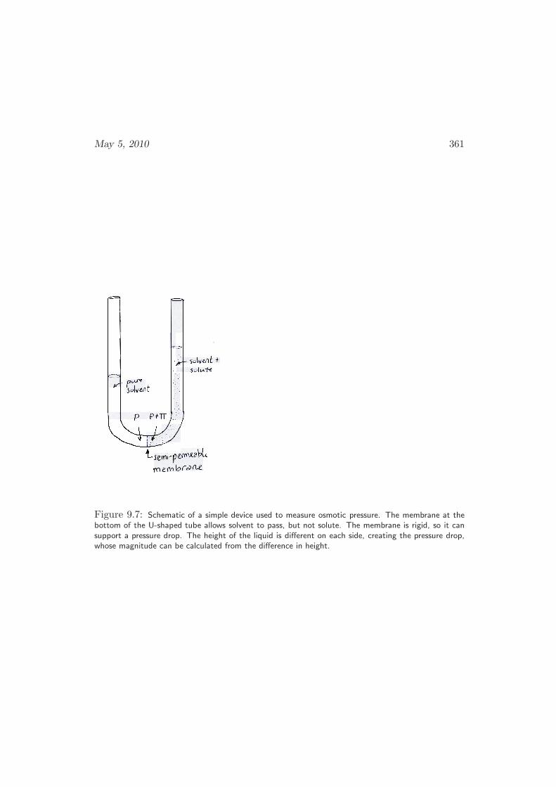
May 5, 2010 361
Figure 9.7: Schematic of a simple device used to measure osmotic pressure. The membrane at thebottom of the U-shaped tube allows solvent to pass, but not solute. The membrane is rigid, so it cansupport a pressure drop. The height of the liquid is different on each side, creating the pressure drop,whose magnitude can be calculated from the difference in height.
362 Chapter 9: Vapor-Liquid Equilibrium
we can write our relation as
log γ1x1 = −∫ P+Π
P
v1[T, P ]
RTdP. (9.93)
If we assume that the specific volume of the pure solvent, v1 doesn’t change appre-ciably in the range [P ;P +Π], Eqn. (9.93) can be simplified to give
Π = −RT log γ1x1v1
. (9.94)
Equation (9.94) can now be used to measure γ1 from knowledge of Π.
9.6 The Blood-Brain Barrier
Human and animal cells are enveloped by membranes. These membranes are rathercomplicated, but are composed primarily of a bilayer of phospholipids. Figure 9.8shows a sketch of a small section of cell membrane. One sees that the bulk ofthe membrane is composed of amphiphilic molecules called phospholipids, whose‘heads’ are hydrophillic (water loving), and whose two ‘tails’ are hydrophobic (wa-ter avoidant). In an aqueous solution, such molecules will naturally, then, form abilayer to keep the tails in a hydrophillic environment, and the heads exposed to thewater. By tuning the degree of hydrophilicity in the head, and the length and struc-ture of the tails, many possible structures are possible, such as bilayers, cylinders,bicontinuous phases, etc. Predicting these structures is a very interesting thermo-dynamics problem, and an area of active research. However, we leave aside theseinteresting questions for the moment. Instead we focus on phospholipids, which arecomposed of two hydrophobic fatty acid tails attached to an alcohol, such as glyc-erol. This alcohol also contains a phosphate group, making this head hydrophillic.There are many sorts of phospholipids, depending on the chemical details, but theyall have this same basic structure.
A given membrane, like that shown in Figure 9.8, made up of phospholipids,forms a barrier to molecules that are hydrophillic, preventing them from passinginto the cell easily. In fact, the other proteins embedded in the membrane wallsare believed to have several functions, including guiding desirable ions through themembrane. On the other hand, certain hydrophobic molecules pass favorably intothe cell walls. Therefore, we expect molecules soluble in the phospholipid tails tohave potential biological impact on animals (e.g., humans). We are interested inpredicting this impact for a given molecule, either because it is a drug, or becauseit may be toxic.
A good thermodynamic mimic for the phospholipid tails, but which does notspontaneously form vesicles, is n-octanol, CH3C7H2OH, since it has approximately
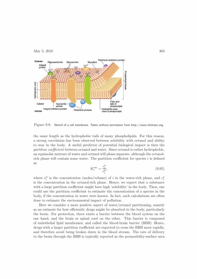
May 5, 2010 363
Figure 9.8: Sketch of a cell membrane. Taken without permission from http://www.chemsoc.org.
the same length as the hydrophobic tails of many phospholipids. For this reason,a strong correlation has been observed between solubility with octanol and abilityto stay in the body. A useful predictor of potential biological impact is then thepartition coefficient between octanol and water. Since octanol is rather hydrophobic,an equimolar mixture of water and octanol will phase separate, although the octanol-rich phase will contain some water. The partition coefficient for species i is definedas
Kowi =
coicwi, (9.95)
where cwi is the concentration (moles/volume) of i in the water-rich phase, and coiis the concentration in the octanol-rich phase. Hence, we expect that a substancewith a large partition coefficient might have high ‘solubility’ in the body. Then, onecould use the partition coefficient to estimate the concentration of a species in thebody, if the concentration in water were known. In fact, such calculations are oftendone to estimate the environmental impact of pollution.
Here we consider a more positive aspect of water/octanol partitioning, namelyas an estimate for how efficiently drugs might be absorbed in the body, particularlythe brain. For protection, there exists a barrier between the blood system on theone hand, and the brain or spinal cord on the other. This barrier is composedof endothelial lipid membranes, and called the blood-brain barrier (BBB). Hence,drugs with a larger partition coefficient are expected to cross the BBB more rapidly,and therefore avoid being broken down in the blood stream. The rate of deliveryto the brain through the BBB is typically reported as the permeability-surface area

364 Chapter 9: Vapor-Liquid Equilibrium
Figure 9.9: Permeability-surface area product [µl/g·min] versus water/octanol partition coefficient(log-log scale). Taken without permission from [67].
product, PS, which has dimensions of (volume drug)/(time × mass brain).Figure 9.9 indeed shows a correlation between the solubility of a drug in octanol,
and its ability to pass the blood-brain barrier. There are important exceptions,however. The drugs that lie above the correlation utilize carrier molecules thatmediate passage through the BBB. The drugs that lie below the line typically havehigher molecular weights, which may make them too large to pass through themembranes. In fact, finding a method to mediate passage through the phospholipidmembranes that make up the barrier is an important area of research for drugdelivery to the brain [68].
9.7 Partial Miscibility
9.7.1 Thermodynamic Stability
Excess properties provide a useful framework to describe partially miscible liquidmixtures. Partial miscibility serves as the basis for many industrial separation pro-cesses; it is therefore important to have a methodology to describe such mixturesquantitatively. This includes calculation of the phase diagrams of binary, ternary,and multicomponent systems.
May 5, 2010 365
As was the case for pure substances, partial miscibility or liquid-liquid phasetransitions in binary mixtures arise as a consequence of thermodynamic instabil-ity. To illustrate this point, it is instructive to recall our previous discussion ofthermodynamic stability for a pure component, in §4.1. There we saw that sec-ond derivatives of potentials with extensive quantities were required to be positive.Therefore, stability also requires
(∂2G
∂N21
)
P,T,N2
≥ 0 (9.96)
For binary mixtures it is often more convenient to work with x1 and x2 asindependent variables rather than N1 and N2. Thus, we wish to cast Eqn. (9.96)in terms of mole fractions instead of mole numbers. In order to do this, we use thechain rule of partial differentiation, Eqn. (A.8), which in this case becomes(
∂
∂N1
)
T,P,N2
=
(∂x1∂N1
)
T,P,N2
(∂
∂x1
)
T,P,N
+
(∂N
∂N1
)
T,P,N2
(∂
∂N
)
T,P,x1
,
=1− x1N
(∂
∂x1
)
T,P,N
+
(∂
∂N
)
T,P,x1
. (9.97)
Hence, we can write(∂G
∂N1
)
T,P,N2
=1− x1N
(∂G
∂x1
)
T,P,N
+
(∂G
∂N
)
T,P,x1
.
= (1− x1)
(∂g
∂x1
)
T,P,N
+ g. (9.98)
To obtain the second line we have exploited the extensivity of the free energy:G(T, P, x1, N) = Ng(T, P, x1). Using the chain rule once more on this result gives
(∂2G
∂N21
)
T,P,N2
=(1− x1)
2
N
(∂2g
∂x21
)
T,P
− 1− x1N
(∂g
∂x1
)
T,P
+
1− x1N
(∂g
∂x1
)
T,P
.
=(1− x1)
2
N
(∂2g
∂x21
)
T,P
(9.99)
A very similar result can be derived for species 2. Hence, we arrive at the simpleresult (
∂2g
∂x2i
)
P,T
> 0, i = 1, 2, locally stable (9.100)
366 Chapter 9: Vapor-Liquid Equilibrium
where the derivative is now taken with respect to the mole fraction (as opposed tothe number of moles).
It is important to emphasize that g in Eqn. (9.100) refers to the free energy ofthe mixture. The total molar Gibbs free energy of a binary mixture can be writtenas the sum of pure component contributions and a free energy change of mixing
gmixture = x1gpure1 + x2g
pure2 +∆gmixing. (9.101)
Note that this equation defines the free energy of mixing, ∆gmixing. Putting thisexpression into Eqn. (9.100) says that thermodynamic stability requires
(∂2∆gmixing
∂x2i
)
P,T
> 0, i = 1, 2, locally stable. (9.102)
Just as for the pure-component case, for given values of temperature and pressure,the point at which Eqn. (9.102) is violated defines the spinodal composition
(∂2∆gmixing
∂x2i
)
P,T
= 0 at spinodal composition. (9.103)
In terms of the excess molar Gibbs free energy, thermodynamic stability is satisfiedwhen (
∂2gE
∂x21
)
P,T
+RT
(1
x1+
1
x2
)
> 0. (9.104)
Figure 9.10 shows the molar Gibbs free energy of mixing predicted by a simpletwo-suffix Margules equation as a function of composition. Three curves are shown:one for which the system is stable at all compositions, one for which the systemstarts to develop an instability, precisely at x = 0.5, and one for which the systemis unstable over a range of compositions. The following example discusses in moredetail the temperature at which the instability first appears.
Example 9.7.1 Consider a binary liquid mixture whose molar excess Gibbs freeenergy can be described by an equation of the form
gE = Ax1x2.
For what values of constant A will the two liquids be miscible?
Solution: The second derivative of the molar excess Gibbs free energy withrespect to mole fraction is given by
(∂2gE
∂x21
)
P,T
= −2A. (9.105)
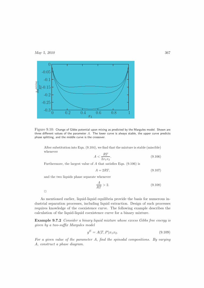
May 5, 2010 367
x1
∆gm
ixin
g
RT
10.80.60.40.20
0
-0.05
-0.1
-0.15
-0.2
-0.25
-0.3
Figure 9.10: Change of Gibbs potential upon mixing as predicted by the Margules model. Shown arethree different values of the parameter A. The lower curve is always stable, the upper curve predictsphase splitting, and the middle curve is the crossover.
After substitution into Eqn. (9.104), we find that the mixture is stable (miscible)whenever
A <RT
2x1x2. (9.106)
Furthermore, the largest value of A that satisfies Eqn. (9.106) is
A = 2RT, (9.107)
and the two liquids phase separate whenever
A
RT> 2. (9.108)
2
As mentioned earlier, liquid-liquid equilibria provide the basis for numerous in-dustrial separation processes, including liquid extraction. Design of such processesrequires knowledge of the coexistence curve. The following example describes thecalculation of the liquid-liquid coexistence curve for a binary mixture.
Example 9.7.2 Consider a binary liquid mixture whose excess Gibbs free energy isgiven by a two-suffix Margules model
gE = A(T, P )x1x2. (9.109)
For a given value of the parameter A, find the spinodal compositions. By varyingA, construct a phase diagram.
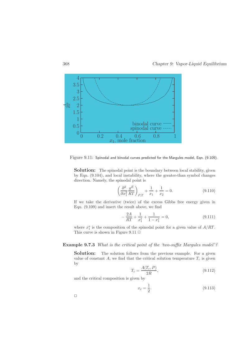
368 Chapter 9: Vapor-Liquid Equilibrium
spinodal curvebinodal curve
x1, mole fraction
A RT
10.80.60.40.20
4
3.5
3
2.5
2
1.5
1
0.5
0
Figure 9.11: Spinodal and binodal curves predicted for the Margules model, Eqn. (9.109).
Solution: The spinodal point is the boundary between local stability, givenby Eqn. (9.104), and local instability, where the greater-than symbol changesdirection. Namely, the spinodal point is
(∂2
∂x21
gE
RT
)
P,T
+1
x1+
1
x2= 0. (9.110)
If we take the derivative (twice) of the excess Gibbs free energy given inEqn. (9.109) and insert the result above, we find
− 2A
RT+
1
xs1+
1
1− xs1= 0, (9.111)
where xs1 is the composition of the spinodal point for a given value of A/RT .This curve is shown in Figure 9.11 2
Example 9.7.3 What is the critical point of the ‘two-suffix Margules model’?
Solution: The solution follows from the previous example. For a givenvalue of constant A, we find that the critical solution temperature Tc is givenby
Tc =A(Tc, P )
2R, (9.112)
and the critical composition is given by
xc =1
2. (9.113)
2
May 5, 2010 369
Example 9.7.4 For a binary liquid mixture whose excess Gibbs free energy is de-scribed by a two-suffix Margules equation, propose a procedure to calculate the coex-istence curve.
Solution: At equilibrium, the fugacity of both components should be thesame in both phases. We can therefore write
f ′1 = f ′′
1
f ′2 = f ′′
2 , (9.114)
where superscripts ′ and ′′ serve to denote the two coexisting phases. Eqs.(9.114)can be written as
x′1γ′1 = x′′1γ
′′1 ,
x′2γ′2 = x′′2γ
′′2 . (9.115)
After substituting expressions for the activity coefficient of a two-suffix Mar-gules equation, we have
x′1 exp(A(1− x′1)
2)
= x′′1 exp
(A(1− x′′1 )
2
RT
)
(1− x′1) exp
(A(x′1)
2
RT
)
= (1− x′′1 ) exp
(
Ax′′12
RT
)
, (9.116)
Eqs. (9.116) and (9.116) are equivalent to each other. They can be simplifiedby recognizing that the two-suffix Margules model is symmetric in composition,and therefore x′1 = 1− x′′1 . With that simplification, we have
x′1 exp
(A(1− x′1)
2
RT
)
= (1− x′1) exp
(
Ax′12
RT
)
, (9.117)
which can now be solved for arbitrary values of A. To make the binodal curve
in Figure 9.11, we can solve this equation for A/RT = log(
1−x′1
x′1
)
/(1− 2x′1) 2
In the previous example, we saw how the composition of two coexisting liquidphases can be calculated by equating the fugacity of each component in each phase.For a binary mixture, it can also be shown that at coexistence, the following relationsare satisfied
(∂∆gmixing
∂x1
)′=
(∂∆gmixing
∂x1
)′′(9.118)
∆gmixing′ − x1′(∂∆gmixing
∂x1
)′= ∆gmixing′′ − x1
′′(∂∆gmixing
∂x1
)′′. (9.119)
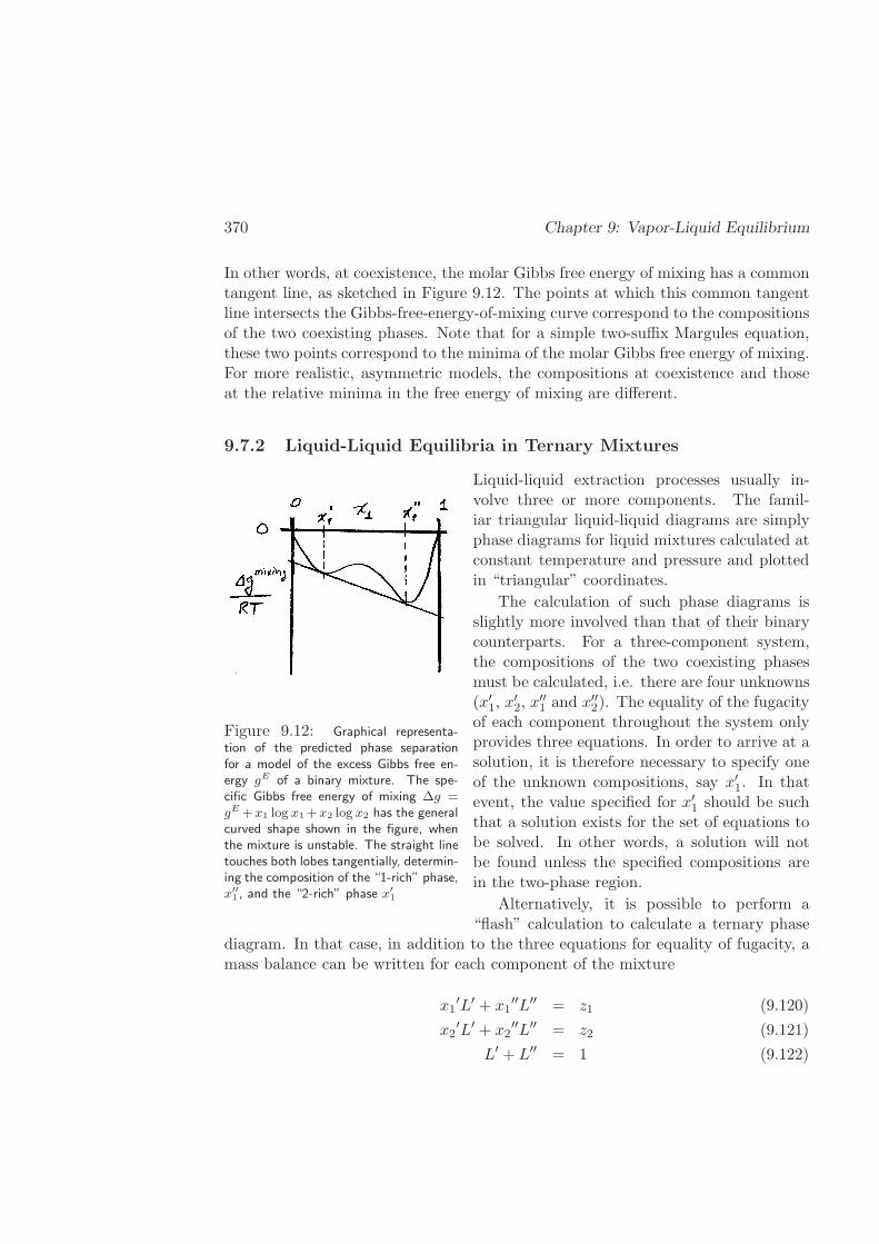
370 Chapter 9: Vapor-Liquid Equilibrium
In other words, at coexistence, the molar Gibbs free energy of mixing has a commontangent line, as sketched in Figure 9.12. The points at which this common tangentline intersects the Gibbs-free-energy-of-mixing curve correspond to the compositionsof the two coexisting phases. Note that for a simple two-suffix Margules equation,these two points correspond to the minima of the molar Gibbs free energy of mixing.For more realistic, asymmetric models, the compositions at coexistence and thoseat the relative minima in the free energy of mixing are different.
9.7.2 Liquid-Liquid Equilibria in Ternary Mixtures
Figure 9.12: Graphical representa-tion of the predicted phase separationfor a model of the excess Gibbs free en-ergy gE of a binary mixture. The spe-cific Gibbs free energy of mixing ∆g =gE+x1 log x1+x2 log x2 has the generalcurved shape shown in the figure, whenthe mixture is unstable. The straight linetouches both lobes tangentially, determin-ing the composition of the “1-rich” phase,x′′1 , and the “2-rich” phase x′
1
Liquid-liquid extraction processes usually in-volve three or more components. The famil-iar triangular liquid-liquid diagrams are simplyphase diagrams for liquid mixtures calculated atconstant temperature and pressure and plottedin “triangular” coordinates.
The calculation of such phase diagrams isslightly more involved than that of their binarycounterparts. For a three-component system,the compositions of the two coexisting phasesmust be calculated, i.e. there are four unknowns(x′1, x
′2, x
′′1 and x′′2). The equality of the fugacity
of each component throughout the system onlyprovides three equations. In order to arrive at asolution, it is therefore necessary to specify oneof the unknown compositions, say x′1. In thatevent, the value specified for x′1 should be suchthat a solution exists for the set of equations tobe solved. In other words, a solution will notbe found unless the specified compositions arein the two-phase region.
Alternatively, it is possible to perform a“flash” calculation to calculate a ternary phase
diagram. In that case, in addition to the three equations for equality of fugacity, amass balance can be written for each component of the mixture
x1′L′ + x1
′′L′′ = z1 (9.120)
x2′L′ + x2
′′L′′ = z2 (9.121)
L′ + L′′ = 1 (9.122)
May 5, 2010 371
where zi denotes the overall (feed) composition of component i, L′ and L′′ arethe total numbers of moles in phases ′ and ′′, respectively, and where the basisfor calculations is one mole of feed mixture. There are now six equations and sixunknowns, namely x′1, x
′2, x
′′1 , x
′′2 , L
′ and L′′.It is interesting to point out that the coexistence curve for a ternary mixture can
be determined through a geometrical construct analogous to that mentioned abovefor binary systems. It can be shown that, at coexistence, the following relations aretrue
(∂∆gmixing
∂x1
)′=
(∂∆gmixing
∂x1
)′′(9.123)
(∂∆gmixing
∂x2
)′=
(∂∆gmixing
∂x2
)′′, (9.124)
and
∆gmixing′ − x1′(∂∆gmixing
∂x1
)′− x2
′(∂∆gmixing
∂x2
)′(9.125)
= ∆gmixing′′ − x1′′(∂∆gmixing
∂x1
)′′− x2
′′(∂∆gmixing
∂x2
)′′.
Eqs.(9.177), (9.178), and (9.179) state that at coexistence the molar Gibbs freeenergy of mixing surface has a common tangent plane. The coexistence curve canbe obtained by rolling a plane over that surface and by projecting the intersectionpoints onto the composition plane.
It is convenient to represent the phases in ternary mixtures using triangular dia-grams of the sort shown in Figure 9.13. The mole fraction of the mixture determinesthe location inside the triangle. The pure components are located at the verticesof the triangle. Note the straight line that runs parallel to the side of the triangleopposite the vertex. The fractional distance from this opposite side to the vertexindicates the mole fraction of that species. The thick curved line is the binodalcurve. Inside this region the mixture separates into two phases–a water-rich phaseand a benzene-rich phase. These two phases are connected by a straight (dashed)tie line.
9.7.3 Critical Points
Just as for the case of thermodynamic stability, an exact correspondence existsbetween the critical point observed in a pure fluid, and the critical points that occurin binary liquid mixtures. For the pure component case we showed that, at the

372 Chapter 9: Vapor-Liquid Equilibrium
Figure 9.13: Ternary diagram for a three component mixture of trimethyl pentane, benzene, andfurfural at T = 25C. The location of a point inside the triangle indicates the mole fraction of eachcomponent. The thick line is the binodal curve, which delineates the region of composition wherethe mixture separates into two phases. The solid squares show experimental data. The straight linesconnecting the data points on the two sides of the binodal (which are in equilibrium with each other) arecalled tie-lines. The binodal curve and the tie lines shown in the figure were calculated using the NRTLmodel. This figure is taken without permission from [Henty C.J., McManamey W.J. Prince R.G.H. J.Appl. Chem. 14 (1964) 148].

May 5, 2010 373
critical point,
(∂P
∂v
)
T
= 0,
(∂2P
∂v2
)
T
= 0.
For a binary liquid mixture, at the critical solution point, we have
(∂2gmixture
∂x2i
)
T,P
= 0, (9.126)
(∂3gmixture
∂x3i
)
T,P
= 0. (9.127)
For any given excess Gibbs free energy model, Eqs.(9.126) and (9.127) can thereforebe used to determine the position of the critical point.
9.8 Simple Free Energy Models from Statistical Me-chanics
Some of the models employed in this chapter can be derived using the methods ofstatistical mechanics. In this section we discuss how to derive Lewis mixing rules,and the Margules equation of state using lattice models. The assumptions necessaryfor these derivations indicate when we can expect these equations to be applicable.
Lattice models are commonly used to describe liquids and solids. In these mod-els, molecules are typically assumed to occupy distinct lattice sites, and the systemof interest is generally assumed to be incompressible (i.e., the volume is constant).This assumption of constant volume makes it easier to work in the canonical ensem-ble (T, V, Ni), instead of the usual grand canonical ensemble (T, P, Ni) of theexcess Gibbs models.
In the simplest case, the lattice can be assumed to be cubic and fully occupied.The coordination number of the lattice, denoted by zl, specifies the number ofnearest neighbors for a lattice site. In two dimensions, each molecule of the systemhas 4 nearest neighbors; in three dimensions each molecule has 6 nearest neighbors.For simplicity, only interactions between nearest-neighbors are considered in thederivations that follow. With these assumptions in mind, we can write the canonicalpartition function as
Q ∼ qAA(T, v)NAAqBB(T, v)
NBBqAB(T, v)NAB (9.128)
374 Chapter 9: Vapor-Liquid Equilibrium
where NAA, NBB and NAB denote the numbers of nearest-neighbor AA, BB or ABpairs. We have also used the pairwise partition functions qij(T, v), for a lattice offixed specific volume.
At this point it is instructive to note that, for a given composition and a givensize of the system, several distinct configurations of the system can have exactly thesame energy. Rather than summing over all distinct configurations of the systemin Eqn. (9.128), we can therefore sum over configurations having a certain numberof AB pairs. The quantity ωd(NA, NB , NAB) is called the degeneracy of thesystem and, for any given composition, it corresponds to the number of distinctarrangements or configurations of the system that have exactly NAB pairs.
For a given composition of the system, the number of AA (or BB) pairs on thelattice is related to the coordination number through
zlNA = 2NAA + NAB (9.129)
zlNB = 2NBB + NAB (9.130)
where NA and NB are the numbers of molecules of type A and type B on the lattice,respectively. Hence, using the degeneracy, and these relations for NAA and NBB ,we can rewrite Eqn. (9.128) as
Q = qAA(T, v)zlNA/2qBB(T, v)
zlNB/2∑
NAB
ωd(NAB)λ(T, v)NAB , (9.131)
whereλ(T, v) := qAB(T, v)/
√
qAA(T, v)qBB(T, v). (9.132)
If we take the logarithm of each side of Eqn. (9.131), and multiply by −kBT , weobtain
F = −1
2zlNART log qAA(T, v) −
1
2zlNBRT log qBB(T, v)
−kBT log
∑
NAB
ωd(NAB , NA, NB)λ(T, v)NAB
, (9.133)
where we used the relationship between the free energy and the partition function,Eqn. (6.12). The first two quantities on the right are the free energies for the purespecies (imagine filling a lattice of the same specific volume with only A and findingthe partition function). Hence, we can rewrite this expression as
F = F pure A(T, v,NA) + F pure B(T, v,NB) + ∆Fmixing(T, v, NA, NB),
(9.134)
May 5, 2010 375
where we have found an expression for the free energy of mixing
∆Fmixing(T, v, NA, NB) = −kBT log
∑
NAB
ωd(NAB , NA, NB)λ(T, v)NAB
.
(9.135)
Note that this is the change of mixing at constant volume instead of at constantpressure, so the equivalence with our earlier models is valid only for incompressiblefluids. At any rate, we have a starting point to find a fundamental F relation forthe mixture.
The problem of estimating the free energy of the system has now been reducedto that of estimating the degeneracy of the system and carrying out the summationappearing in Eqn. (9.135). At this point, it is necessary to introduce approximationsthat will allow us to produce such estimates.
9.8.1 Lewis mixing
As a starting point, we consider the case for which qAB(T, v) =√
qAA(T, v)qBB(T, v),so that λ(T, v) = 1. In this case, the interactions of an AB pair are the same, onaverage, as those of an AA pair and a BB pair. For such a mixture we have
∆Fmixing(T, v, NA, NB) = −kBT log
∑
NAB
ωd(NAB, NA, NB)
(9.136)
The summation in Eqn. (9.136) represents the total number of ways of arrangingNA and NB objects randomly on precisely N = NA + NB lattice sites; as such, it isgiven by (see Appendix A.8)
∑
NAB
ωd(NA, NB , NAB) =N !
NA!NB !. (9.137)
The Helmholtz free energy of the random mixture is therefore given by
∆Fmixing(T, v, NA, NB) = −kBT log
[
(NA + NB)!
NA!NB !
]
(9.138)
This last equation can be simplified by invoking Stirling’s approximation, whichstates that for sufficiently large values of N , the natural logarithm of a factorialnumber can be approximated according to
logN ! ≈ N logN −N. (9.139)
376 Chapter 9: Vapor-Liquid Equilibrium
We can therefore rewrite (9.138) as
∆Fmixing(T, v, xA, xB)
NRT∼= xA log xA + xB log xB . (9.140)
This result shows that the free energy of a mixture with no change in the energiesof interactions upon mixing corresponds to a Lewis mixture. The difference is thatLewis mixing defined by Eqn. (8.66) in purely macroscopic terms resorted to Lewis’fugacity rule. The random mixture considered here therefore provides a molecu-lar foundation for some of the concepts introduced earlier using phenomenologicalarguments.
9.8.2 Margules Model
We can now go beyond the random (or Lewis) mixture by introducing the ideaof a “mean field.” To first order, we could assume that the number of AB pairsappearing in the exponential of Eqn. (9.135) can be replaced by its average or meanvalue for a random mixture. Furthermore, we could assume that the degeneracyfunction ωd(NA, NB , NAB) can be approximated by that corresponding to a randommixture. If we use N∗
AB to denote this random mean value, we have
∆Fmixing(T, v, NA, NB) ∼= −kBT log
∑
NAB
ωd(NAB, NA, NB)λ(T, v)N∗AB
.
= −kBT log
λ(T, v)N∗AB
∑
NAB
ωd(NAB , NA, NB)
.
= −kBT log
[
λ(T, v)N∗AB
(NA + NB)!
NA!NB !
]
.
= −N∗ABkBT log λ(T, v) + kBT
(
NA log xA + NB log xB
)
.
(9.141)
The second term on the right hand side of Eqn. (9.141) is given by Eqn. (9.137). Thefirst term can be evaluated using probabilistic arguments. We have NA A moleculeson the lattice. Each one of these has zl adjacent sites. The probability that one ofthese sites has a B molecule is NB/N , if the molecules are distributed randomly.Therefore, the number of AB pairs is estimated to be
N∗AB = NAzl
NB
N(9.142)
May 5, 2010 377
This simplification is called the random phase approximation. The averagenumber of AB pairs for a random mixture is therefore given by
N∗AB = zl
NANB
NA + NB
. (9.143)
After a few algebraic manipulations, Eqn. (9.141) can be rewritten in terms of molefractions as
∆Fmixing
NRT= xA log xA + xB log xB − zl log
(
qAB(T, v)√
qAA(T, v)qBB(T, v)
)
xAxB. (9.144)
which is the expression introduced earlier (within our constant-volume assumption)as the “two-suffix Margules” equation using purely phenomenological arguments,with A/RT = −zl log
[qAB/
√qAAqBB
].
9.8.3 Exact Solution of Lattice Model
The simple theory outlined above can be refined systematically by eliminating orimproving some of the approximations involved in the derivation of Eqn. (9.144).In the exercises is another analytic approach called the “quasi-chemical approxima-tion.” Alternatively, one can solve the equation numerically using a Monte Carlosimulation. Those refinements, however, are beyond the scope of this text, andinterested readers are referred to the original literature on the subject.
9.9 Summary
This chapter introduces the student to concepts necessary for predicting the thermo-dynamic properties, particularly equilibrium compositions, of multiphase miscibleand partially miscible liquid mixtures. A student should now be able to performvapor-liquid, liquid-liquid, or solid-liquid phase equilibrium calculations using theconcepts put forth in this chapter.
• We introduced the concept of excess properties, ME , Eqn. (9.2), to quantifydeviations from Lewis (or ideal) mixing behavior:
ME(T, P, Ni) =M(T, P, Ni)−MLewis(T, P, Ni)
• The molar excess Gibbs free energy gE was introduced as a useful means todefine activity coefficients:
log γi :=gEiRT
.
378 Chapter 9: Vapor-Liquid Equilibrium
• The general phase-equilibrium problem for an r-component system can nowbe stated in terms of fugacity coefficients (for a vapor, fluid phase or liquidphase) and activity coefficients (for a condensed phase) according to:
xiγifpurei = yiφiP, i = 1, ..., r.
• Several models of GE(T, P, Ni) can be used to predict activities in mixtures.In particular, we considered the Margules Model in some detail. However,other models, such as van Laar’s, Wilson’s, NRTL, and the UNIQUAC modelwere introduced in §9.4. Using these models, the student should be able topredict compositions of liquid and vapor phases in equilibrium. We also dis-cussed how several experiments, including the measurement of freezing pointsor osmotic pressure, could be used to determine activity coefficients.
• In §9.5 we introduced Henry’s Law for phase-equilibrium problems involvingdilute components (e.g., gases) in liquid mixtures. Temperature and pressuredependence of the Henry’s Law constant, Hi,j were also found. Hence, ther-modynamic data are used to predict changes in solubility with temperatureand pressure. As an example, the solubility of nitrogen in water was predictedas a function of pressure.
• We introduced the concept of the octanol-water partition coefficient, and howit could be used to predict the ability of specific chemical compounds to crossthe blood-brain barrier. Drugs for treating the brain must be able to passthrough this barrier, whereas organic toxins are potentially more hazardouswhen they have a large water/octanol partition coefficient.
• Some liquids are not completely miscible. Section 9.7 illustrates how to useexcess molar Gibbs free energy models to predict miscibility of binary andternary mixtures. Given such a model, the student should be able to predictthe coexistence curve and spinodal curve for a binary, ternary, or multicom-ponent mixture of species. The resulting binary and ternary diagrams areessential for design of liquid-liquid extraction processes.
• The final section of the chapter shows how some of the simpler excess Gibbsmodels can be derived using a lattice model from statistical mechanics. Thatsection is important for understanding the molecular origins (and the assump-tions) of specific models for GE , which in §9.4 were introduced in purely em-pirical terms.
May 5, 2010 379
9.10 Exercises
9.3.A: Show that the activity coefficient of component 1 of a binary mixture can beobtained from the following relation
RT log γ1 = gE + x2
(∂gE
∂x1
)
T,P
(9.145)
9.3.B: Derive Eqn.(9.19).
9.3.C: Derive an expression for the molar excess enthalpy of mixing of a mixturedescribed by a molar excess Gibbs free energy of the form
gE = x1x2(A21x1 +A12x2) (9.146)
where constants A21 and A12 are independent of temperature.
9.3.D: For a ternary mixture, the simplest version of the Margules equation takesthe form
gE
RT= A12x1x2 +A13x1x3 +A23x2x3 (9.147)
where the Aij are adjustable parameters determined from binary data for the ijpair. Show that the activity coefficients of components 1, 2 and 3 are given by
log γ1 = A12x22 +A13x
23 + (A12 +A13 −A23)x2x3 (9.148)
log γ2 = A12x21 +A23x
23 + (A12 +A23 −A13)x1x3 (9.149)
log γ3 = A13x21 +A23x
22 + (A13 +A23 −A12)x1x2 (9.150)
9.3.E: Show that the activity coefficients corresponding to Eqn. (9.31) are of theform:
RT log γ1 = a′x22 + b′x32 + c′x42 + d′x52 + ...
RT log γ2 = a′′x21 + b′′x31 + c′′x41 + d′′x51 + ... (9.151)
where the lower case constants are related to those appearing in Eqn. (9.31) through:
a′ = A+ 3B + 5C + 7D
a′′ = A− 3B − 5C − 7D
b′ = −4B − 16C − 36D
b′′ = 4B − 16C + 36D
c′ = 12C + 60D
c′′ = 12C − 60D
d′ = −32D
d′′ = 32D
380 Chapter 9: Vapor-Liquid Equilibrium
9.3.F: Show that, for a binary azeotropic mixture at constant pressure, the tem-perature at the azeotrope corresponds to the maximum or the minimum of thetemperature-composition curve.
9.3.G: Derive Eqs.(9.13) and (9.14).
9.3.H: The molar excess Gibbs free energy for the Flory-Huggins model Eqn. (11.1)can be written as
gE
RT= xs log
φsxs
+ xp logφpxp
+ χ(xs + rpxp)φsφp , (9.152)
where the volume fractions of the solvent and polymer are given by
φs =xs
xs + rpxpφp =
rpxpxs + rpxp
, (9.153)
where rp = vp/vs provides a measure of the asymmetry between the volume of thepolymer and solvent molecules.
1. Experimental data for the solubility of polystyrene in methylcyclohexane in-dicate that this mixture exhibits partial miscibility. Show that the criticalvolume fraction and the critical χ parameter are given by
φc =1
1 +√rp
(9.154)
χc =1
2
(
1 +1√rp
)2
. (9.155)
2. Show that, for the Flory-Huggins model, the activity coefficient of the solventcan be written as
log γs = logφsxs
+
(
1− 1
rp
)
φp + χφ2p , (9.156)
where φs is the volume fraction of the solvent.
3. For a molecular weight ofMw = 4.64×10⁴, this mixture first becomes partiallyimmiscible at a temperature of T = 40C and a volume fraction of the polymerφ = 0.13. Calculate the solvent partial pressure above a 60%wt polystyrenesolution in methylcyclohexane at 320 K.
Data: the molar volume of methylcyclohexane is approximately 88 cm3/mol.Its molecular weight is 99 g/mol, and its vapor pressure is P sat = 0.13 bar
May 5, 2010 381
at T =298 K, and P sat = 0.24 bar at T =312K, respectively. The molecularweight of a polymer segment in polystyrene is 106, and the volume of themonomer is approximately 150 cm3/mol. If you cannot calculate χ or areuncertain about your result, perform your calculations assuming χ = 1.
9.3.I: Biological molecules (such as amino acids or proteins) and heat-sensitive hy-drocarbons are often purified by crystallization processes. Design of such processesrequires precise knowledge of the activity of the liquid in equilibrium with the solid.This problem considers the thermodynamics of solid-liquid equilibria.
1) Show that the “fugacity ratio” of a pure substance (the ratio of the solid andthe supercooled-liquid fugacity) is given by an expression of the form:
log
(
f solidi
f liquidi
)
=∆hi,melting
RTt,i
(Tt,iT
− 1
)
− ∆Cp,iR
(Tt,iT
− 1
)
+∆Cp,iR
log
(Tt,iT
)
(9.157)where ∆hi,melting is the enthalpy change of melting of component i, and ∆Cp,i is thedifference in the molar heat capacity of supercooled liquid i and solid i at the sametemperature, i.e. ∆Cp = C liquid
p − Csolidp . In Eqn. (9.157) T denotes the tempera-
ture at which the fugacity ratio is being evaluated, and Tt,i denotes the triple pointtemperature of i.
(Hint: Eqn. (9.157) can be derived by constructing a thermodynamic cycle consist-ing of the following three steps:
• Cool solid from temperature of interest (T ) to triple point temperature (Tt).
• Melt the solid into a liquid at the triple point temperature.
• Heat the supercooled liquid from the triple point temperature to the temper-ature of interest.
For each of these processes, one can evaluate the change in free energy, noting thatg = h− Ts. )
2) Derive an expression for the ideal solubility of a solid solute in a liquid solvent(an expression that assumes that the liquid phase is ideal).
3) Experimental data (see below) are available for the solubility of glucose andsucrose in water at T = 343K. For simplicity, the excess molar Gibbs free energy
382 Chapter 9: Vapor-Liquid Equilibrium
of this ternary mixture in the liquid phase can be described by an expression of theform
gE
RT= A12x1x2 +A13x1x3 +A23x2x3 . (9.158)
Please determine appropriate values for parameters Aij . You may assume thatsucrose and glucose form pure solids. You may also assume that the terms involvingthe heat capacity in Equation (9.157) can be neglected. To a first approximation, youcan also replace the triple-point temperature in Equation (9.157) with the meltingtemperature Tm to get
log
(
f solidi
f liquidi
)
≈ ∆hi,melting
RTi,m
(Ti,mT
− 1
)
. (9.159)
Data: The enthalpy change of melting for glucose (1) and sucrose (2) are ∆h1,melting =32.4 kJ/mol and ∆h2,melting = 46.2 kJ/mol. The melting temperatures are T1,m =423 K and T2,m = 460 K. At T = 343 K the solubility of glucose in pure wateris x1 = 0.259 and the solubility of sucrose in pure water is x2 = 0.146. Whenx1 = 0.123, the solubility of sucrose is x2 = 0.118.
9.3.J: The so-called van’t Hove equation stipulates a linear dependence of the os-motic pressure on concentration and temperature:
Π = CRT (9.160)
Please provide a derivation of this equation and clearly indicate under which as-sumptions or in which limit it is justified.
9.4.A: Show that for a two-parameter Margules equation for the molar excess Gibbsfree energy,
gE = x1x2(A21x1 +A12x2) (9.161)
the activity coefficients of components 1 and 2 are given by
log γ1 =1
RT
[x22A12 + 2x1(A21 −A12)
](9.162)
log γ2 =1
RT
[x21A21 + 2x2(A12 −A21)
](9.163)
9.4.B: Show that, at infinite dilution, the activity coefficients of a binary mixturedescribed by Wilson’s equation are given by
log γ∞1 = 1− log Λ12 − Λ21 (9.164)
log γ∞2 = 1− log Λ21 − Λ12 (9.165)
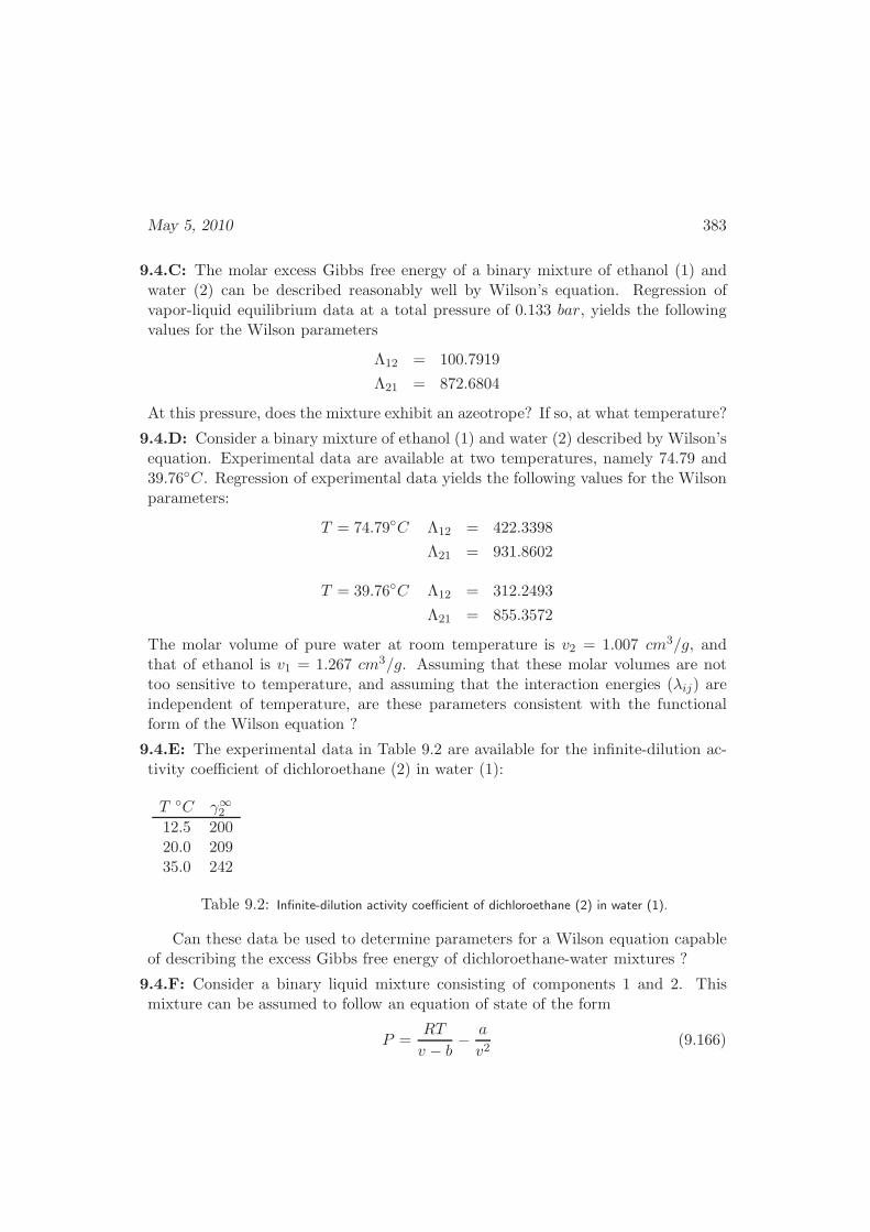
May 5, 2010 383
9.4.C: The molar excess Gibbs free energy of a binary mixture of ethanol (1) andwater (2) can be described reasonably well by Wilson’s equation. Regression ofvapor-liquid equilibrium data at a total pressure of 0.133 bar, yields the followingvalues for the Wilson parameters
Λ12 = 100.7919
Λ21 = 872.6804
At this pressure, does the mixture exhibit an azeotrope? If so, at what temperature?
9.4.D: Consider a binary mixture of ethanol (1) and water (2) described by Wilson’sequation. Experimental data are available at two temperatures, namely 74.79 and39.76C. Regression of experimental data yields the following values for the Wilsonparameters:
T = 74.79C Λ12 = 422.3398
Λ21 = 931.8602
T = 39.76C Λ12 = 312.2493
Λ21 = 855.3572
The molar volume of pure water at room temperature is v2 = 1.007 cm3/g, andthat of ethanol is v1 = 1.267 cm3/g. Assuming that these molar volumes are nottoo sensitive to temperature, and assuming that the interaction energies (λij) areindependent of temperature, are these parameters consistent with the functionalform of the Wilson equation ?
9.4.E: The experimental data in Table 9.2 are available for the infinite-dilution ac-tivity coefficient of dichloroethane (2) in water (1):
T C γ∞212.5 20020.0 20935.0 242
Table 9.2: Infinite-dilution activity coefficient of dichloroethane (2) in water (1).
Can these data be used to determine parameters for a Wilson equation capableof describing the excess Gibbs free energy of dichloroethane-water mixtures ?
9.4.F: Consider a binary liquid mixture consisting of components 1 and 2. Thismixture can be assumed to follow an equation of state of the form
P =RT
v − b− a
v2(9.166)

384 Chapter 9: Vapor-Liquid Equilibrium
with mixing rules given by
a = a1x21 + a2x
22 + 2x1x2
√a1a2(1− k12) (9.167)
b = x1b1 + x2b2. (9.168)
Parameter k12 in Eqn. (9.167) depends on the nature of the mixture; it is intendedto account for deviations from a geometric-mean combining rule. Assuming thatboth the molar excess volume of mixing and the molar excess entropy of mixing arenegligible, derive an expression for the molar excess free energy of such a mixture.(Hint: describe the mixing process by devising a three-step thermodynamic cyclethat comprises expansion of the two pure liquids, mixing of the resulting gases, andcompression of the gas mixture into a liquid state. Evaluate the internal energycorresponding to each of the three steps by using the equation of state above.)
9.4.G: Table 9.3, provides VLE data for the system methanol(1)/2-methyl-1-propanol(2)at 60C (extracted from Udovenko V. V., Frid TS. B., ZH. FIZ. KHIM., 22, 1135(1948)).
Pressure (mm Hg) x1 y196.00 0.0 0.000163.90 0.1 0.471227.40 0.2 0.660287.10 0.3 0.761342.50 0.4 0.827394.80 0.5 0.873443.70 0.6 0.908490.40 0.7 0.936535.70 0.8 0.960579.60 0.9 0.981620.00 1.0 1.000
Table 9.3: Experimental Data for the system methanol(1)/2-methyl-1-propanol(2) at 60C
The Antoine equation, Eqn. (4.49) can be used to correlate vapor pressures. Theconstants for each of the two components in this problem are provided in Table 9.4,where P sat
i is the vapor pressure of pure component i (in mm Hg) and T is thetemperature (in C).
1. Find parameters for the van Laar equation that provide a best fit to theexperimental vapor phase composition. Prepare a Pxy diagram that comparesthe experimental data with the curves determined from the calculations.
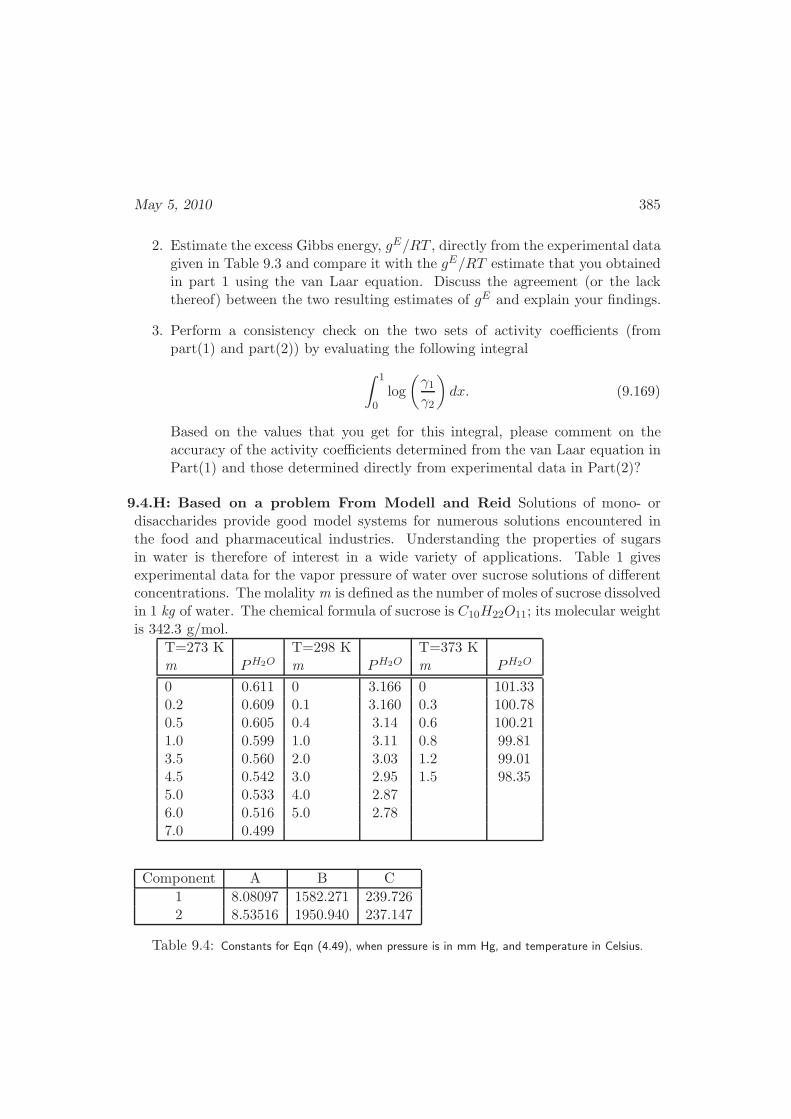
May 5, 2010 385
2. Estimate the excess Gibbs energy, gE/RT , directly from the experimental datagiven in Table 9.3 and compare it with the gE/RT estimate that you obtainedin part 1 using the van Laar equation. Discuss the agreement (or the lackthereof) between the two resulting estimates of gE and explain your findings.
3. Perform a consistency check on the two sets of activity coefficients (frompart(1) and part(2)) by evaluating the following integral
∫ 1
0log
(γ1γ2
)
dx. (9.169)
Based on the values that you get for this integral, please comment on theaccuracy of the activity coefficients determined from the van Laar equation inPart(1) and those determined directly from experimental data in Part(2)?
9.4.H: Based on a problem From Modell and Reid Solutions of mono- ordisaccharides provide good model systems for numerous solutions encountered inthe food and pharmaceutical industries. Understanding the properties of sugarsin water is therefore of interest in a wide variety of applications. Table 1 givesexperimental data for the vapor pressure of water over sucrose solutions of differentconcentrations. The molalitym is defined as the number of moles of sucrose dissolvedin 1 kg of water. The chemical formula of sucrose is C10H22O11; its molecular weightis 342.3 g/mol.
T=273 K T=298 K T=373 Km PH2O m PH2O m PH2O
0 0.611 0 3.166 0 101.330.2 0.609 0.1 3.160 0.3 100.780.5 0.605 0.4 3.14 0.6 100.211.0 0.599 1.0 3.11 0.8 99.813.5 0.560 2.0 3.03 1.2 99.014.5 0.542 3.0 2.95 1.5 98.355.0 0.533 4.0 2.876.0 0.516 5.0 2.787.0 0.499
Component A B C
1 8.08097 1582.271 239.7262 8.53516 1950.940 237.147
Table 9.4: Constants for Eqn (4.49), when pressure is in mm Hg, and temperature in Celsius.
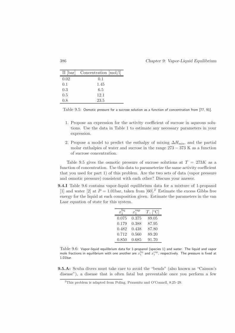
386 Chapter 9: Vapor-Liquid Equilibrium
Π [bar] Concentration [mol/l]
0.02 0.10.1 1.450.3 6.50.5 12.10.8 23.5
Table 9.5: Osmotic pressure for a sucrose solution as a function of concentration from [77, 91].
1. Propose an expression for the activity coefficient of sucrose in aqueous solu-tions. Use the data in Table 1 to estimate any necessary parameters in yourexpression.
2. Propose a model to predict the enthalpy of mixing ∆Hmix, and the partialmolar enthalpies of water and sucrose in the range 273 − 373 K as a functionof sucrose concentration.
Table 9.5 gives the osmotic pressure of sucrose solutions at T = 273K as afunction of concentration. Use this data to parameterize the same activity coefficientthat you used for part 1) of this problem. Are the two sets of data (vapor pressureand osmotic pressure) consistent with each other? Discuss your answer.
9.4.I Table 9.6 contains vapor-liquid equilibrium data for a mixture of 1-propanol[1] and water [2] at P = 1.01bar, taken from [60].2 Estimate the excess Gibbs freeenergy for the liquid at each composition given. Estimate the parameters in the vanLaar equation of state for this system.
xliq1 xvap1 T , [C]
0.075 0.375 89.050.179 0.388 87.950.482 0.438 87.800.712 0.560 89.200.850 0.685 91.70
Table 9.6: Vapor-liquid equilibrium data for 1-propanol (species 1) and water. The liquid and vapormole fractions in equilibrium with one another are xliq
1 and xvap1 , respectively. The pressure is fixed at
1.01bar.
9.5.A: Scuba divers must take care to avoid the “bends” (also known as “Caisson’sdisease”), a disease that is often fatal but preventable once you perform a few
2This problem is adapted from Poling, Prausnitz and O’Connell, 8.25–29.
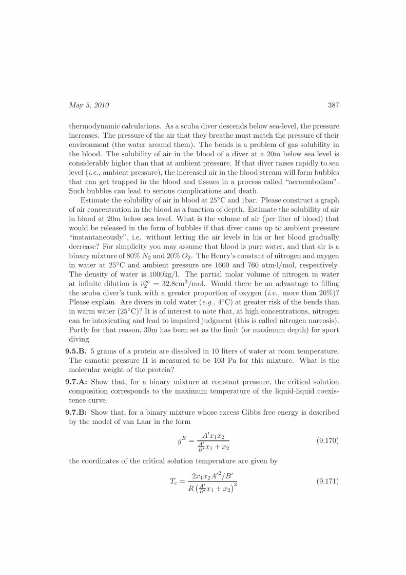
May 5, 2010 387
thermodynamic calculations. As a scuba diver descends below sea-level, the pressureincreases. The pressure of the air that they breathe must match the pressure of theirenvironment (the water around them). The bends is a problem of gas solubility inthe blood. The solubility of air in the blood of a diver at a 20m below sea level isconsiderably higher than that at ambient pressure. If that diver raises rapidly to sealevel (i.e., ambient pressure), the increased air in the blood stream will form bubblesthat can get trapped in the blood and tissues in a process called “aeroembolism”.Such bubbles can lead to serious complications and death.
Estimate the solubility of air in blood at 25C and 1bar. Please construct a graphof air concentration in the blood as a function of depth. Estimate the solubility of airin blood at 20m below sea level. What is the volume of air (per liter of blood) thatwould be released in the form of bubbles if that diver came up to ambient pressure“instantaneously”, i.e. without letting the air levels in his or her blood graduallydecrease? For simplicity you may assume that blood is pure water, and that air is abinary mixture of 80% N2 and 20% O2. The Henry’s constant of nitrogen and oxygenin water at 25C and ambient pressure are 1600 and 760 atm·l/mol, respectively.The density of water is 1000kg/l. The partial molar volume of nitrogen in waterat infinite dilution is v∞2 = 32.8cm3/mol. Would there be an advantage to fillingthe scuba diver’s tank with a greater proportion of oxygen (i.e., more than 20%)?Please explain. Are divers in cold water (e.g., 4C) at greater risk of the bends thanin warm water (25C)? It is of interest to note that, at high concentrations, nitrogencan be intoxicating and lead to impaired judgment (this is called nitrogen narcosis).Partly for that reason, 30m has been set as the limit (or maximum depth) for sportdiving.
9.5.B. 5 grams of a protein are dissolved in 10 liters of water at room temperature.The osmotic pressure Π is measured to be 103 Pa for this mixture. What is themolecular weight of the protein?
9.7.A: Show that, for a binary mixture at constant pressure, the critical solutioncomposition corresponds to the maximum temperature of the liquid-liquid coexis-tence curve.
9.7.B: Show that, for a binary mixture whose excess Gibbs free energy is describedby the model of van Laar in the form
gE =A′x1x2
A′B′x1 + x2
(9.170)
the coordinates of the critical solution temperature are given by
Tc =2x1x2A
′2/B′
R(A′B′x1 + x2
)3 (9.171)
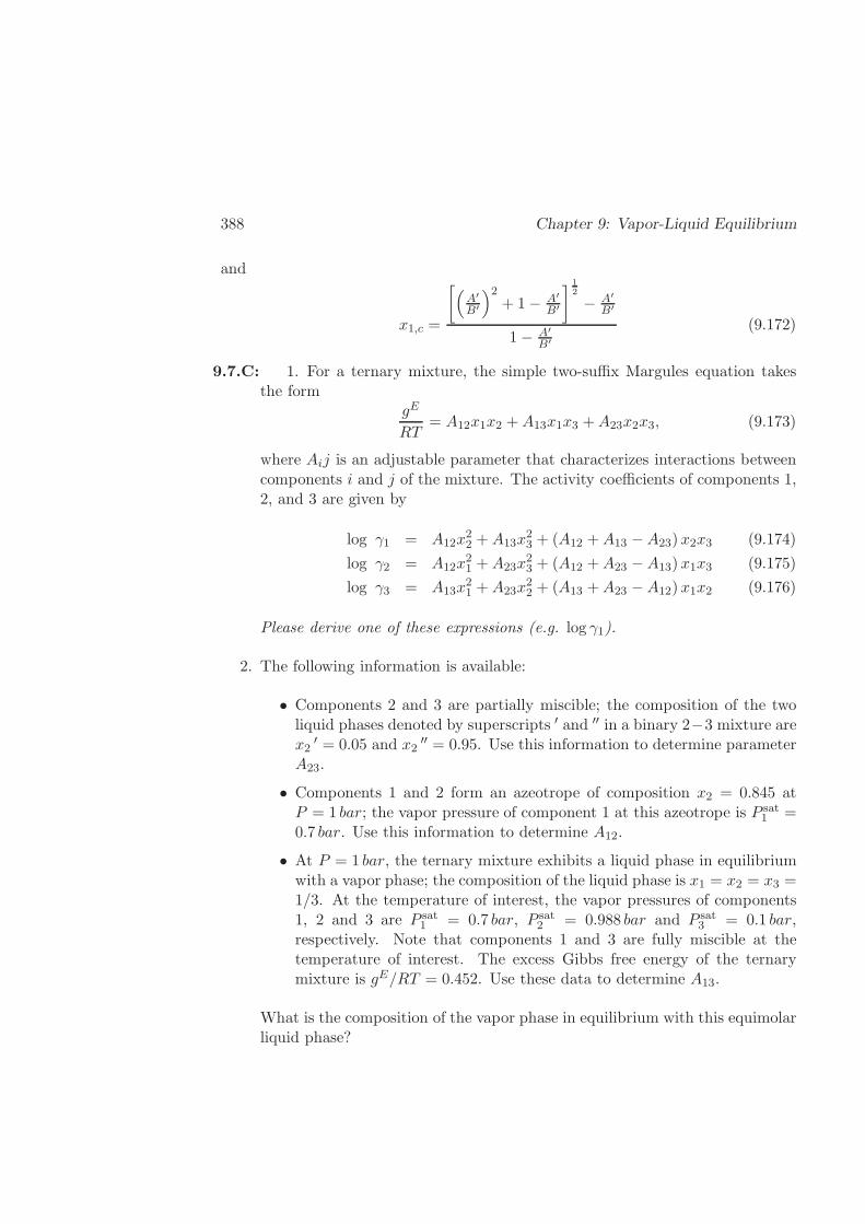
388 Chapter 9: Vapor-Liquid Equilibrium
and
x1,c =
[(A′B′
)2+ 1− A′
B′
] 12
− A′B′
1− A′B′
(9.172)
9.7.C: 1. For a ternary mixture, the simple two-suffix Margules equation takesthe form
gE
RT= A12x1x2 +A13x1x3 +A23x2x3, (9.173)
where Aij is an adjustable parameter that characterizes interactions betweencomponents i and j of the mixture. The activity coefficients of components 1,2, and 3 are given by
log γ1 = A12x22 +A13x
23 + (A12 +A13 −A23) x2x3 (9.174)
log γ2 = A12x21 +A23x
23 + (A12 +A23 −A13) x1x3 (9.175)
log γ3 = A13x21 +A23x
22 + (A13 +A23 −A12) x1x2 (9.176)
Please derive one of these expressions (e.g. log γ1).
2. The following information is available:
• Components 2 and 3 are partially miscible; the composition of the twoliquid phases denoted by superscripts ′ and ′′ in a binary 2−3 mixture arex2
′ = 0.05 and x2′′ = 0.95. Use this information to determine parameter
A23.
• Components 1 and 2 form an azeotrope of composition x2 = 0.845 atP = 1 bar; the vapor pressure of component 1 at this azeotrope is P sat
1 =0.7 bar. Use this information to determine A12.
• At P = 1 bar, the ternary mixture exhibits a liquid phase in equilibriumwith a vapor phase; the composition of the liquid phase is x1 = x2 = x3 =1/3. At the temperature of interest, the vapor pressures of components1, 2 and 3 are P sat
1 = 0.7 bar, P sat2 = 0.988 bar and P sat
3 = 0.1 bar,respectively. Note that components 1 and 3 are fully miscible at thetemperature of interest. The excess Gibbs free energy of the ternarymixture is gE/RT = 0.452. Use these data to determine A13.
What is the composition of the vapor phase in equilibrium with this equimolarliquid phase?
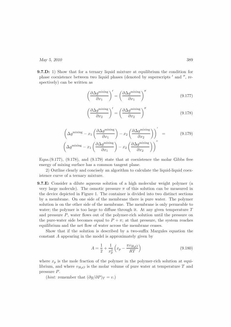
May 5, 2010 389
9.7.D: 1) Show that for a ternary liquid mixture at equilibrium the condition forphase coexistence between two liquid phases (denoted by superscripts ′ and ′′, re-spectively) can be written as
(∂∆gmixing
∂x1
)′=
(∂∆gmixing
∂x1
)′′(9.177)
(∂∆gmixing
∂x2
)′=
(∂∆gmixing
∂x2
)′′(9.178)
(
∆gmixing − x1
(∂∆gmixing
∂x1
)
− x2
(∂∆gmixing
∂x2
))′
= (9.179)
(
∆gmixing − x1
(∂∆gmixing
∂x1
)
− x2
(∂∆gmixing
∂x2
))′′
Eqns.(9.177), (9.178), and (9.179) state that at coexistence the molar Gibbs freeenergy of mixing surface has a common tangent plane.
2) Outline clearly and concisely an algorithm to calculate the liquid-liquid coex-istence curve of a ternary mixture.
9.7.E: Consider a dilute aqueous solution of a high molecular weight polymer (avery large molecule). The osmotic pressure π of this solution can be measured inthe device depicted in Figure 1. The container is divided into two distinct sectionsby a membrane. On one side of the membrane there is pure water. The polymersolution is on the other side of the membrane. The membrane is only permeable towater; the polymer is too large to diffuse through it. At any given temperature Tand pressure P , water flows out of the polymer-rich solution until the pressure onthe pure-water side becomes equal to P + π; at that pressure, the system reachesequilibrium and the net flow of water across the membrane ceases.
Show that if the solution is described by a two-suffix Margules equation theconstant A appearing in the model is approximately given by
A =1
2+
1
x2p
(
xp −πvH2O
RT
)
(9.180)
where xp is the mole fraction of the polymer in the polymer-rich solution at equi-librium, and where vH2O is the molar volume of pure water at temperature T andpressure P .
(hint: remember that (∂g/∂P )T = v.)
390 Chapter 9: Vapor-Liquid Equilibrium
9.8.A Another approximation to the lattice model considered in §9.8 is called thequasi-chemical approximation. Rather than assume that N∗
AB is well estimated bythe random-phase approximation, we assume that it can be estimated from some-thing like a chemical equilibrium equation
NAANBB(
N∗AB
)2 =1
4
(q2AB
qAAqBB
)
. (9.181)
This expression incorporates the idea that unfavorable energetics for AB interactions(compared to AA and BB energetics) leads to a decrease in the number of AB pairs.
Using the quasi-chemical approximation, find the predicted excess Gibbs poten-tial. From this potential make a plot of the spinodal and binodal curves as functions
of χ(T ) := 14
(q2AB
qAAqBB
)
.
Chapter 10
Reaction Equilibrium
Reactions are an essential component of chemical engineering, and reaction engi-neering represents a very broad discipline itself [33, 75]. However, before we studythe time evolution of chemical reactions, it is important to know the final equilib-rium state that a system can reach. The equilibrium state of a chemical reaction isdetermined by thermodynamic principles.
In this chapter we examine the thermodynamic principles that govern chemicalreactions, and find methods for calculating the final composition of a mixture thatresults from chemical reactions. The methods consist of two general steps: deter-mination of the equilibrium constant(s) from thermodynamic properties of the con-stituent chemical compounds, and; determination of the chemical composition of theequilibrium mixture from the initial composition, and the equilibrium constant(s).In general, finding this composition requires using models with good estimates forthe activities (or fugacities) of the constituent species, as shown in the previoustwo chapters. The equilibrium constant depends only on the temperature, and thespecies present, and not on composition.
We also consider how thermodynamic driving forces can influence reaction rates.However, few details are given in this book, since that is a topic best left for othercourses and textbooks. Denaturation of DNA strands are also discussed in §10.9,where denaturation is applied to polymerase chain reactions (PCR). PCR is a tech-nique to amplify small amounts of genetic material. Finally, in the last section,§10.10, connections are made to statistical mechanics.
10.1 A Simple Picture: The Reaction Coordinate
Before constructing the rigorous mathematical machinery necessary to solve prob-lems, we introduce a simplified picture to aid our thinking about kinetics and the
391
392 Chapter 10: Reactions
equilibrium composition of reacting systems. We start with the simple, first-orderreaction
A B, (10.1)
but the picture applies to second-order reactions as well.We imagine that the molecule A must go through some changes to become
molecule B. For example, bonds might be strained and broken, or bond anglesmight be modified. These intermediate states must have a higher energy than thestate A, otherwise the reaction would be instantaneous. These changes might bevery complicated, but we characterize the path by a single number called the reac-tion coordinate. Therefore, we draw the simple picture shown in Figure 10.1. Thereaction coordinate is typically the path of minimum free energy between the reac-tants and the products. However, real reactions may fluctuate around this path, orthere may even be multiple paths.
As you can see from this sketch, the same arguments apply for the reversereaction from B to A. This simple picture leads to three simple predictions, all ofwhich are qualitatively correct.
Our first observation is that we expect to have both A and B molecules presentat equilibrium. If the energy barrier is not too high, we expect thermal fluctua-tions experienced by the molecules to cause molecules to constantly go back andforth across the barrier. From statistical mechanics, we know that the probabil-ity for a molecule to be in a given energetic state E (see §6.2) is proportional toexp(−E/kBT ). Therefore, from our sketch, Figure 10.1, we can sketch the proba-bility for a single molecule to have a given reaction coordinate. We sketch this ideain Figure 10.2. Any molecule with reaction coordinate to the left of the barrier iscalled molecule A. From statistical mechanics, we have then
NA
NB
= exp
[EB − EA
kBT
]
, (10.2)
where EA is the energy of one molecule of A.Our second prediction comes from the idea that the rate of the reaction A →
B depends upon the height of the energy barrier to be overcome. Some simplecalculations outside the scope of this text [103] suggest that the rate of a singlemolecule to overcome the barrier is also proportional to the exponential of theheight
“rate of one molecule A→ B” ∼ exp
[Ebarrier − EA
kBT
]
. (10.3)
This rate for a single molecule can be multiplied by the number of molecules NA
to get the total rate of molecules A going to B per unit time. Of course, the sameargument applies for the reverse reaction.
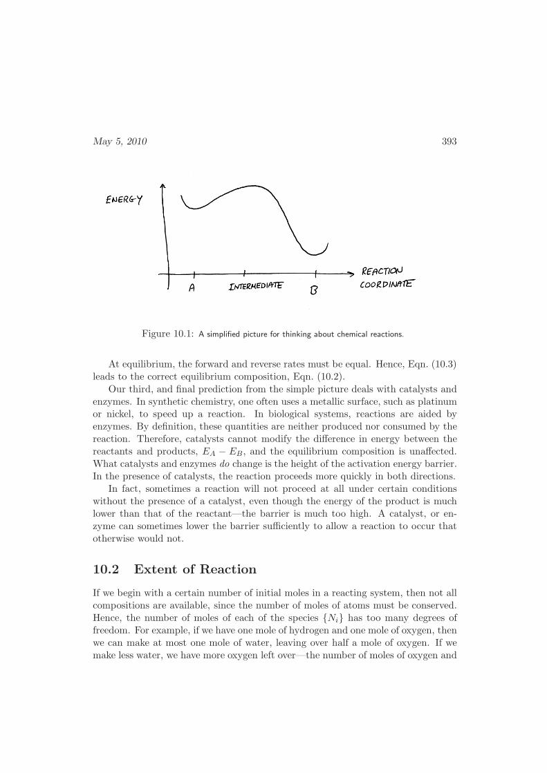
May 5, 2010 393
Figure 10.1: A simplified picture for thinking about chemical reactions.
At equilibrium, the forward and reverse rates must be equal. Hence, Eqn. (10.3)leads to the correct equilibrium composition, Eqn. (10.2).
Our third, and final prediction from the simple picture deals with catalysts andenzymes. In synthetic chemistry, one often uses a metallic surface, such as platinumor nickel, to speed up a reaction. In biological systems, reactions are aided byenzymes. By definition, these quantities are neither produced nor consumed by thereaction. Therefore, catalysts cannot modify the difference in energy between thereactants and products, EA − EB , and the equilibrium composition is unaffected.What catalysts and enzymes do change is the height of the activation energy barrier.In the presence of catalysts, the reaction proceeds more quickly in both directions.
In fact, sometimes a reaction will not proceed at all under certain conditionswithout the presence of a catalyst, even though the energy of the product is muchlower than that of the reactant—the barrier is much too high. A catalyst, or en-zyme can sometimes lower the barrier sufficiently to allow a reaction to occur thatotherwise would not.
10.2 Extent of Reaction
If we begin with a certain number of initial moles in a reacting system, then not allcompositions are available, since the number of moles of atoms must be conserved.Hence, the number of moles of each of the species Ni has too many degrees offreedom. For example, if we have one mole of hydrogen and one mole of oxygen, thenwe can make at most one mole of water, leaving over half a mole of oxygen. If wemake less water, we have more oxygen left over—the number of moles of oxygen and
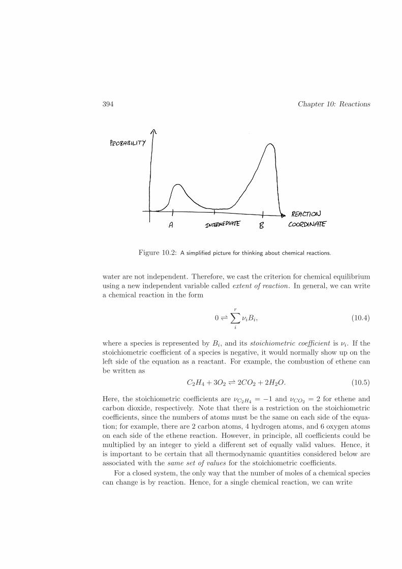
394 Chapter 10: Reactions
Figure 10.2: A simplified picture for thinking about chemical reactions.
water are not independent. Therefore, we cast the criterion for chemical equilibriumusing a new independent variable called extent of reaction. In general, we can writea chemical reaction in the form
0
r∑
i
νiBi, (10.4)
where a species is represented by Bi, and its stoichiometric coefficient is νi. If thestoichiometric coefficient of a species is negative, it would normally show up on theleft side of the equation as a reactant. For example, the combustion of ethene canbe written as
C2H4 + 3O2 2CO2 + 2H2O. (10.5)
Here, the stoichiometric coefficients are νC2H4 = −1 and νCO2 = 2 for ethene andcarbon dioxide, respectively. Note that there is a restriction on the stoichiometriccoefficients, since the numbers of atoms must be the same on each side of the equa-tion; for example, there are 2 carbon atoms, 4 hydrogen atoms, and 6 oxygen atomson each side of the ethene reaction. However, in principle, all coefficients could bemultiplied by an integer to yield a different set of equally valid values. Hence, itis important to be certain that all thermodynamic quantities considered below areassociated with the same set of values for the stoichiometric coefficients.
For a closed system, the only way that the number of moles of a chemical speciescan change is by reaction. Hence, for a single chemical reaction, we can write
May 5, 2010 395
dN1
ν1=dN2
ν2= . . . =
dNm
νm=: dε, single reaction (10.6)
which defines the extent of reaction ε, for a single reaction. The extent of reactionis typically (though arbitrarily) taken to be zero when the components are mixed.Hence, if we integrate just one of the equations above dNi = νiε from the point ofmixing, to some other time, we obtain
Ni = Ni,0 + νiε, (10.7)
where Ni,0 is the initial, non-equilibrium number of moles of species i.If the reaction is taking place in a single phase, we can sum Eqn. (10.7) over all
species to find the total number of moles
NT = NT,0 + εν, single phase (10.8)
where we define ν as
ν :=
r∑
i=1
νi. (10.9)
Again, if we are working in a single phase, we can divide Eqn. (10.7) by Eqn. (10.8)to find the mole fraction of species i
xi =Ni,0 + νiε
NT,0 + νε, single phase, single reaction. (10.10)
If there are q simultaneous reactions taking place in the phase, then we can writeq reactions:
0
r∑
i
ν1i Bi, 0
r∑
i
ν2i Bi, . . . , 0
r∑
i
νqiBi. (10.11)
The change in mole number for species i is now the result of all the reactions, so wecan write
dNi = ν1i dε1 + ν2i dε2 + . . .+ νqi dεq =
q∑
j=1
νji dεj ,
→ Ni = Ni,0 +
q∑
j=1
νji εj . (10.12)
where εj is the extent of reaction j. The last line, as above, is found by integrationfrom the initial state. Now, instead of working with the number of moles of thespecies, we can work with the extents of reaction to ensure that atoms are conserved,and we are working with the minimum number of degrees of freedom necessary.
396 Chapter 10: Reactions
Example 10.2.1 Assuming that the reaction given in Eqn. (10.5) occurs in thegas phase, find the mole fractions of each component as a function of the extent ofreaction.
Solution: For convenience, we rename the components as B1 ≡ C2H4, B2 ≡O2, B3 ≡ CO2, and B4 ≡ H2O. Then, the mole balance equation (10.7) be-comes
N1 = N1,0 − ε
N2 = N2,0 − 3ε
N3 = N3,0 + 2ε
N4 = N4,0 + 2ε. (10.13)
Summing these four equations, we obtain the total number of moles in the gasphase
NT = N1,0 +N2,0 +N3,0 +N4,0 ≡ NT,0. (10.14)
For this example, the total number of moles in the gas phase does not change.Therefore, if we divide each side of Eqn. (10.13) by each side of Eqn. (10.14),we find the composition of the reacting phase as a function of the extent ofreaction
x1 =N1,0 − ε
N1,0 +N2,0 +N3,0 +N4,0,
x2 =N2,0 − 3ε
N1,0 +N2,0 +N3,0 +N4,0,
x3 =N3,0 + 2ε
N1,0 +N2,0 +N3,0 +N4,0,
x4 =N4,0 + 2ε
N1,0 +N2,0 +N3,0 +N4,0. (10.15)
2
10.3 Equilibrium Criterion
Consider a reaction taking place in a system that is in contact with a thermal andpressure reservoir. For constrained temperature and pressure, we have already seenin §3.2 that the Gibbs potential of the system is minimized. Hence, for constant Tand P , Eqn. (3.51) becomes
dG =
r∑
i=1
µidNi
=
(r∑
i=1
µiνi
)
dε, single reaction, (10.16)
May 5, 2010 397
where we have used Eqn. (10.6) to obtain the second line. The minimization re-quirement at equilibrium for the Gibbs potential leads to
(∂G
∂ε
)
T,P
=r∑
i=1
µiνi = 0. (10.17)
Eqn. (10.17) states that the reaction proceeds until the Gibbs potential is minimized;we can predict satisfaction of the criterion by studying the chemical potentials ofall the species.
If there are multiple reactions, G must be minimized with respect to all theextents of reaction (
∂G
∂εi
)
T,P,εj 6=i= 0, i = 1, 2, . . . q. (10.18)
Note that these last two results apply only for an isothermal and isobaric system. Anisolated system would maximize the entropy instead of minimizing G, for example.
10.4 The Reaction Equilibrium Constant
From §8.4, 8.5, and 8.6, we know that we can also find chemical potentials fromestimation of fugacities, fugacity coefficients, and activity coefficients. For reactions,it is customary and convenient to use the activity ai(T, P ) of species i through thefollowing. First, we define the standard reference state to be the pure substance atP ref = 1 bar, and, if the species is a gas at this pressure, as an ideal gas. Note thatthis reference state, which we shall denote by the superscript () is at arbitrarilyspecified temperature. Then, from the definition of fugacity, Eqn. (8.41), we canwrite the chemical potential relative to this reference state as
ai :=fi(T, P, xi)fpurei (T, P ref)
=
(xiP
P ref
)
exp
[µi(T, P, xi)− µideali (T, P, xi)
RT
]
×
exp
[
−µpurei (T, P ref)− µpure,ideali (T, P ref)
RT
]
=
(xiP
P ref
)
exp
[µi(T, P, xi)− µpurei (T, P ref)−RT log(xiP/P
ref)
RT
]
= exp
[µi(T, P, xi)− µpurei (T, P ref)
RT
]
, (10.19)
398 Chapter 10: Reactions
and taking the logarithm of each side. To obtain the second line, we used thedefinition of fugacities. We used the expression for the chemical potential of amixture of ideal gases to obtain the third line, and the properties of logarithm toobtain the fourth.
The equilibrium criterion can be written in terms of activity by substitutingEqn. (10.19) into Eqn. (10.17). After a bit of algebra, we arrive at the equilibriumcriterion in the form
r∏
i=1
aνii = K(T ), equilibrium criterion, single reaction (10.20)
where we define the equilibrium constant K as
K(T ) := exp
(
−∆g
RT
)
, (10.21)
and the standard Gibbs free energy change of reaction
∆g(T ) :=r∑
i=1
νiµi , (10.22)
where µi := µpurei [P ref ]. These are now the rigorous results for a system held atfixed temperature and pressure, to replace the qualitative results from §10.1. Insteadof mole number, the activity is important, and instead of energy differences, freeenergy differences determine the equilibrium composition.
For solving problems, our task is now split into two parts: first we find theequilibrium constant K from Eqs. (10.21) and (10.22), which is a function of onlytemperature and which species are present; once we know K, we determine thecompositions that give the activities satisfying Eqn. (10.20). It is important to usethe same reference state for finding ∆g or K as is used for the activities.
Methods for finding K are discussed in §10.6, and methods of finding composi-tions based on K are discussed in §10.7.
10.5 Standard Property Changes
Beside the standard Gibbs free energy change, it is convenient to define a generalstandard property change for property M
May 5, 2010 399
∆M :=∑
i
νiMi . (10.23)
Of particular importance in reactions are the standard enthalpy changes ∆H, andthe standard entropy changes ∆S. Note that the standard enthalpy change isequivalent to the standard heat of reaction used in reaction energy balances. Forexample, from the definition of the standard enthalpy change, and the Gibbs-Duhemrelation (8.17), we can write
∆H
RT 2=
∑
i
νiHi
RT 2
= −∑
i
νid
dT
(Gi
RT
)
= − d
dT
(∑
i
νiGi
RT
)
= − d
dT
(∆G
RT
)
=d
dTlogK. (10.24)
The fourth line follows from the definition of ∆G, and the last line follows fromthe definition of K.
We can make several useful observations based on Eqn. (10.24).
• Eqn. (10.24) provides a relatively easy means to calculate the standard heatof reaction by measuring the equilibrium constant at several temperatures.
• If ∆H < 0, then the enthalpy of the products is smaller than the enthalpy ofthe reactants. Hence, energy is released and the reaction is called exother-mic. From Eqn. (10.24) we see that the equilibrium constant for exothermicreactions decreases when the temperature is raised. The opposite is true forendothermic reactions: raising the temperature increases the equilibriumconstant. Hence, one should lower the temperature of exothermic reactions toincrease yield, and raise the temperature of endothermic ones.1
• If the heat of reaction is already known, Eqn. (10.24) can be used to estimatethe temperature dependence of the equilibrium constant, by approximating∆H as constant.
1It is sometimes claimed that this is an example of LeChatelier’s Principle. However, noresults from stability analysis are necessary to arrive at the conclusion.
400 Chapter 10: Reactions
10.6 Estimating the Equilibrium Constant
To estimate the equilibrium constant, Eqn. (10.21), it is necessary to find the stan-dard Gibbs free energy change of reaction at the temperature of interest. From thedefinition of ∆G, we need the chemical potentials for each component at the stan-dard pressure, and the reaction temperature. If we choose pure elements in theirnatural state at a standard pressure of P ref = 1 bar as a reference state, we can find∆G from the Gibbs free energy of formation of each compound.
Example 10.6.1 Consider the ethene reaction given in Eqn. (10.5). Find the cor-responding standard change in Gibbs free energy from the energy of formation ofeach compound.
Solution: We can write this reaction as the sum of the four reactions offormation of each of the species present
−1× ( 2C(s) + 2H2(g) C2H4 )+2× ( C(s) +O2(g) CO2 )+2× ( H2(g) +
12O2(g) H2O )
−3× ( O2(g) O2(g) )C2H4 + 3O2 2CO2 + 2H2O,
(10.25)
Note that we simply multiply the formation reaction by the stoichiometriccoefficient of the compound, and add the result to the sum. In an analogousway, we can add up the standard property changes for each of the formationreactions
−1× ( ∆gf (C2H4) = µC2H4
− 2µC − 2µ
H2)
+2× ( ∆gf (CO2) = µCO2
− µC − µ
O2)
+2× ( ∆gf (H2O) = µH2O
− µH2
− 12µ
O2
)−3× ( ∆gf (O2) = µ
O2= 0 )
(10.26)
∆g = 2∆gf (CO2) + 2∆gf (H2O) −∆gf (C2H4)− 3∆gf (O2),
It is important to point out that the free energy of formation usually tabulated(such as in §D.2) are also at a reference temperature. Hence, the standard freeenergy change found above would be valid at that temperature only.2
The general construction is a straightforward generalization of Eqn. (10.26)
∆M =∑
i
νi∆Mf,i. (10.27)
May 5, 2010 401
If values for the Gibbs free energy of formation are tabulated, we can use Eqn. (10.27)with M ≡ G directly. Or, if values for H and S are tabulated at some standardtemperature T0, we can use the definition of G
∆G(T ) =∑
i
νi∆Gf,i(T )
=∑
i
νi(∆Hf,i(T )− T∆S
f,i(T ))
= ∆H(T )− T∆S(T ). (10.28)
Usually, standard property changes of formation are tabulated not only at a standardpressure, but at a standard temperature T ref as well (such as in §D.2), whereaswe may need the equilibrium constant at arbitrary temperature T . In order tofind the standard change of Gibbs free energy at arbitrary temperature T insteadof the standard tabulated temperature T ref , we may use the heat capacity of theconstituents and Eqn. (10.28)
∆G[T ] =∑
i
νi[∆H
f,i[T ]− T∆Sf,i[T ]
]
=∑
i
νi
[
∆Hf,i[T
ref ] +
∫ T
T ref
CP,i[T′]dT ′
−TSi [T
ref ]− T
∫ T
T ref
CP,i[T′]
T ′ dT ′]
= ∆G[T ref ]− (T − T ref)∆S[T ref ]
+
∫ T
T ref
(T ′ − T
T ′
)
∆CP [T
′]dT ′, (10.29)
where ∆CP [T
′] :=∑
i νiCP,i[T′, P ref ]. For the reference pressure used here (P ref =
1bar), ideal heat capacities can be used for gases.
Example 10.6.2 For the chemical vapor deposition of solid silicon in semiconduc-tor manufacturing, the decomposition of silane is used at elevated temperatures
SiH4 Si(s) + 2H2, (10.30)
where, when not indicated otherwise, components are gases. However, there are alsotwo undesirable side reactions that can occur
SiH4 SiH2 +H2
SiH4 + SiH2 Si2H6 (10.31)
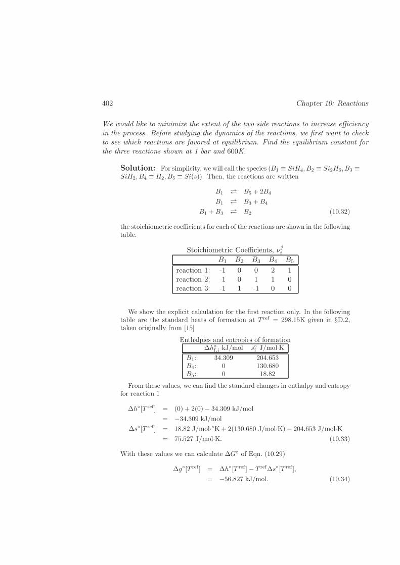
402 Chapter 10: Reactions
We would like to minimize the extent of the two side reactions to increase efficiencyin the process. Before studying the dynamics of the reactions, we first want to checkto see which reactions are favored at equilibrium. Find the equilibrium constant forthe three reactions shown at 1 bar and 600K.
Solution: For simplicity, we will call the species (B1 ≡ SiH4, B2 ≡ Si2H6, B3 ≡SiH2, B4 ≡ H2, B5 ≡ Si(s)). Then, the reactions are written
B1 B5 + 2B4
B1 B3 +B4
B1 +B3 B2 (10.32)
the stoichiometric coefficients for each of the reactions are shown in the followingtable.
Stoichiometric Coefficients, νjiB1 B2 B3 B4 B5
reaction 1: -1 0 0 2 1reaction 2: -1 0 1 1 0reaction 3: -1 1 -1 0 0
We show the explicit calculation for the first reaction only. In the followingtable are the standard heats of formation at T ref = 298.15K given in §D.2,taken originally from [15]
Enthalpies and entropies of formation∆hf,i kJ/mol si J/mol·K
B1: 34.309 204.653B4: 0 130.680B5: 0 18.82
From these values, we can find the standard changes in enthalpy and entropyfor reaction 1
∆h[T ref ] = (0) + 2(0)− 34.309 kJ/mol
= −34.309 kJ/mol
∆s[T ref ] = 18.82 J/mol·K+ 2(130.680 J/mol·K)− 204.653 J/mol·K= 75.527 J/mol·K. (10.33)
With these values we can calculate ∆G of Eqn. (10.29)
∆g[T ref ] = ∆h[T ref ]− T ref∆s[T ref ],
= −56.827 kJ/mol. (10.34)
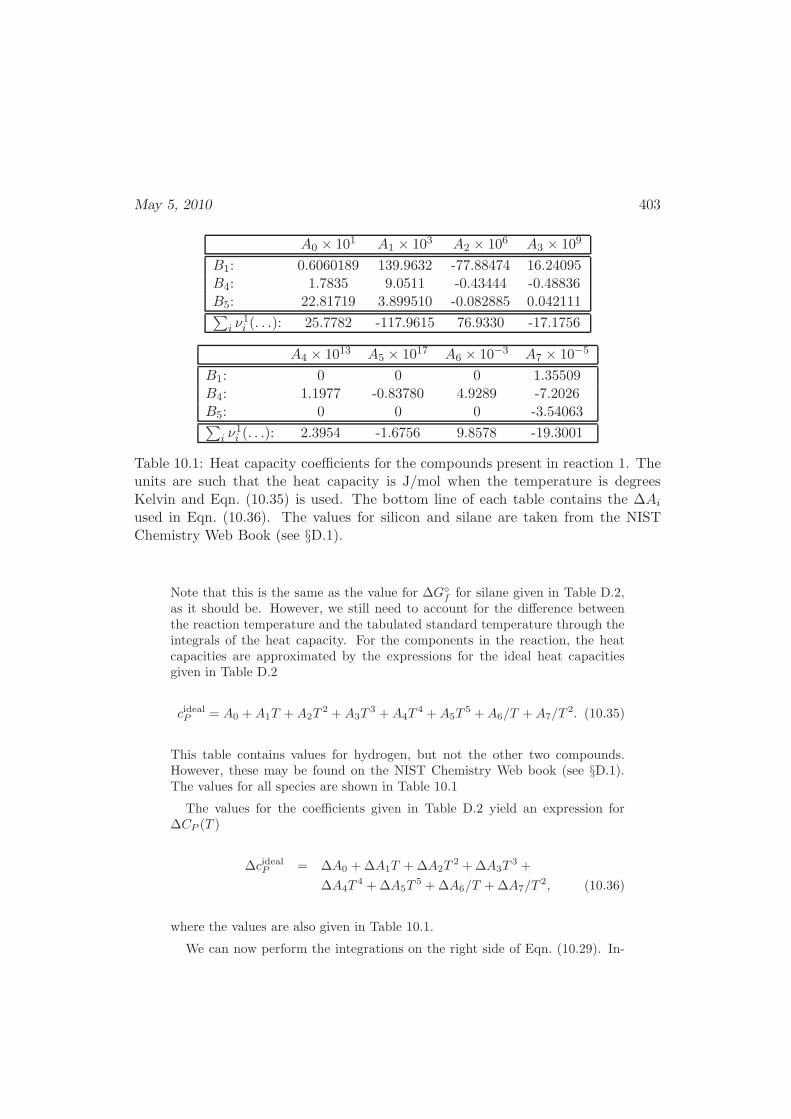
May 5, 2010 403
A0 × 101 A1 × 103 A2 × 106 A3 × 109
B1: 0.6060189 139.9632 -77.88474 16.24095B4: 1.7835 9.0511 -0.43444 -0.48836B5: 22.81719 3.899510 -0.082885 0.042111∑
i ν1i (. . .): 25.7782 -117.9615 76.9330 -17.1756
A4 × 1013 A5 × 1017 A6 × 10−3 A7 × 10−5
B1: 0 0 0 1.35509B4: 1.1977 -0.83780 4.9289 -7.2026B5: 0 0 0 -3.54063∑
i ν1i (. . .): 2.3954 -1.6756 9.8578 -19.3001
Table 10.1: Heat capacity coefficients for the compounds present in reaction 1. Theunits are such that the heat capacity is J/mol when the temperature is degreesKelvin and Eqn. (10.35) is used. The bottom line of each table contains the ∆Aiused in Eqn. (10.36). The values for silicon and silane are taken from the NISTChemistry Web Book (see §D.1).
Note that this is the same as the value for ∆Gf for silane given in Table D.2,
as it should be. However, we still need to account for the difference betweenthe reaction temperature and the tabulated standard temperature through theintegrals of the heat capacity. For the components in the reaction, the heatcapacities are approximated by the expressions for the ideal heat capacitiesgiven in Table D.2
cidealP = A0 +A1T +A2T2 + A3T
3 +A4T4 +A5T
5 +A6/T +A7/T2. (10.35)
This table contains values for hydrogen, but not the other two compounds.However, these may be found on the NIST Chemistry Web book (see §D.1).The values for all species are shown in Table 10.1
The values for the coefficients given in Table D.2 yield an expression for∆CP (T )
∆cidealP = ∆A0 +∆A1T +∆A2T2 +∆A3T
3 +
∆A4T4 +∆A5T
5 +∆A6/T +∆A7/T2, (10.36)
where the values are also given in Table 10.1.
We can now perform the integrations on the right side of Eqn. (10.29). In-

404 Chapter 10: Reactions
serting Eqn. (10.36) into the integral in Eqn. (10.29), we obtain
∫ T
T ref
(T ′ − T
T ′
)
∆cidealP (T ′)dT ′ = (∆A0 − T∆A1)(T − T ref
)+
(∆A1 − T∆A2)1
2
(T 2 − (T ref)2
)+
(∆A2 − T∆A3)1
3
(T 3 − (T ref)3
)+
(∆A3 − T∆A4)1
4
(T 4 − (T ref)4
)+
(∆A4 − T∆A5)1
5
(T 5 − (T ref)5
)+
∆A51
6
(T 6 − (T ref)6
)+
(∆A6 − T∆A0) log(T/T ref
)+
(
∆A6 −∆A7
T
)(
1− T
T ref
)
+
1
2T∆A7
(1
T 2− 1
(T ref)2
)
= −925.88 J/mol (10.37)
Inserting this result and the results shown in Eqn. (10.33) into Eqn. (10.29),we find that
∆g[T = 600K] = −80.863kJ/mol. (10.38)
From the definition of the equilibrium constant, Eqn. (10.21), we can then find
K[T = 600K] = 10.96× 10⁶, (10.39)
which indicates that the reaction is extremely favorable. Under most reactorconditions, the reaction does not proceed anywhere close to its equilibriumcomposition.
2
10.7 Determination of Equilibrium Compositions
Once we have determined the equilibrium constants for the possible reactions in asystem, we use Eqn. (10.20) to determine the compositions. Therefore, we requireuseful expressions for the activities. Fortunately, these have already been found in
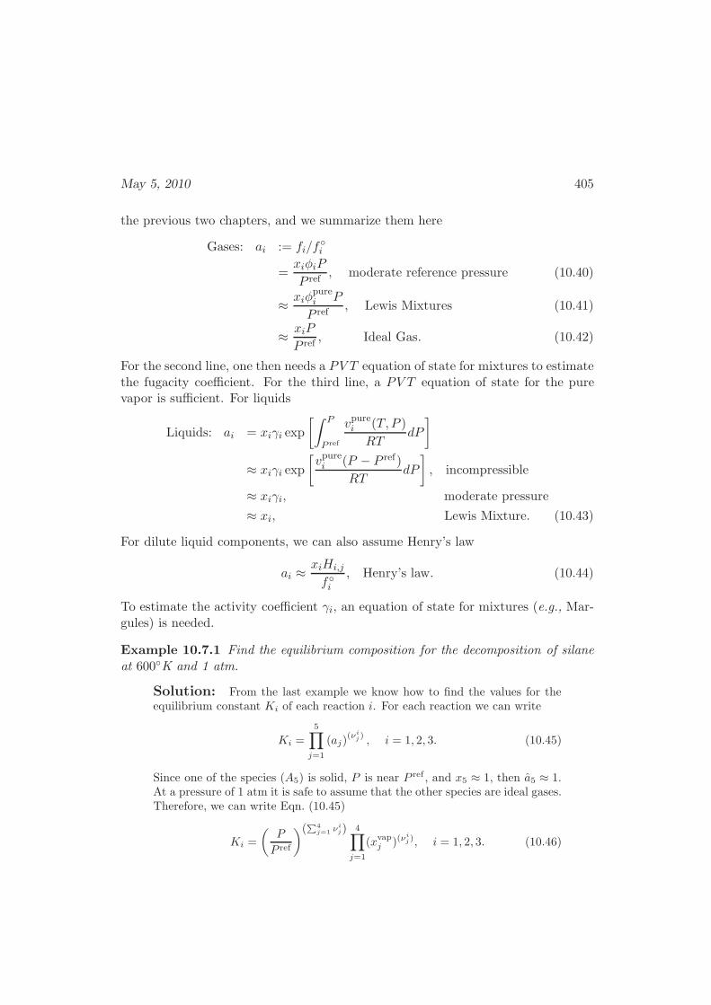
May 5, 2010 405
the previous two chapters, and we summarize them here
Gases: ai := fi/fi
=xiφiP
P ref, moderate reference pressure (10.40)
≈ xiφpurei P
P ref, Lewis Mixtures (10.41)
≈ xiP
P ref, Ideal Gas. (10.42)
For the second line, one then needs a PV T equation of state for mixtures to estimatethe fugacity coefficient. For the third line, a PV T equation of state for the purevapor is sufficient. For liquids
Liquids: ai = xiγi exp
[∫ P
P ref
vpurei (T, P )
RTdP
]
≈ xiγi exp
[vpurei (P − P ref)
RTdP
]
, incompressible
≈ xiγi, moderate pressure
≈ xi, Lewis Mixture. (10.43)
For dilute liquid components, we can also assume Henry’s law
ai ≈xiHi,j
fi, Henry’s law. (10.44)
To estimate the activity coefficient γi, an equation of state for mixtures (e.g., Mar-gules) is needed.
Example 10.7.1 Find the equilibrium composition for the decomposition of silaneat 600K and 1 atm.
Solution: From the last example we know how to find the values for theequilibrium constant Ki of each reaction i. For each reaction we can write
Ki =5∏
j=1
(aj)(νi
j) , i = 1, 2, 3. (10.45)
Since one of the species (A5) is solid, P is near P ref , and x5 ≈ 1, then a5 ≈ 1.At a pressure of 1 atm it is safe to assume that the other species are ideal gases.Therefore, we can write Eqn. (10.45)
Ki =
(P
P ref
)(∑4
j=1 νij) 4∏
j=1
(xvapj )(νij), i = 1, 2, 3. (10.46)
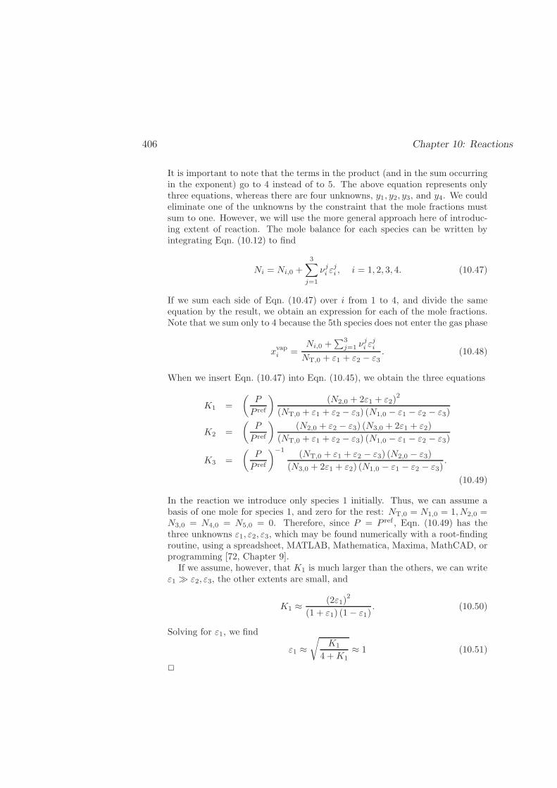
406 Chapter 10: Reactions
It is important to note that the terms in the product (and in the sum occurringin the exponent) go to 4 instead of to 5. The above equation represents onlythree equations, whereas there are four unknowns, y1, y2, y3, and y4. We couldeliminate one of the unknowns by the constraint that the mole fractions mustsum to one. However, we will use the more general approach here of introduc-ing extent of reaction. The mole balance for each species can be written byintegrating Eqn. (10.12) to find
Ni = Ni,0 +
3∑
j=1
νji εji , i = 1, 2, 3, 4. (10.47)
If we sum each side of Eqn. (10.47) over i from 1 to 4, and divide the sameequation by the result, we obtain an expression for each of the mole fractions.Note that we sum only to 4 because the 5th species does not enter the gas phase
xvapi =Ni,0 +
∑3j=1 ν
ji εji
NT,0 + ε1 + ε2 − ε3. (10.48)
When we insert Eqn. (10.47) into Eqn. (10.45), we obtain the three equations
K1 =
(P
P ref
)(N2,0 + 2ε1 + ε2)
2
(NT,0 + ε1 + ε2 − ε3) (N1,0 − ε1 − ε2 − ε3)
K2 =
(P
P ref
)(N2,0 + ε2 − ε3) (N3,0 + 2ε1 + ε2)
(NT,0 + ε1 + ε2 − ε3) (N1,0 − ε1 − ε2 − ε3)
K3 =
(P
P ref
)−1(NT,0 + ε1 + ε2 − ε3) (N2,0 − ε3)
(N3,0 + 2ε1 + ε2) (N1,0 − ε1 − ε2 − ε3).
(10.49)
In the reaction we introduce only species 1 initially. Thus, we can assume abasis of one mole for species 1, and zero for the rest: NT,0 = N1,0 = 1, N2,0 =N3,0 = N4,0 = N5,0 = 0. Therefore, since P = P ref , Eqn. (10.49) has thethree unknowns ε1, ε2, ε3, which may be found numerically with a root-findingroutine, using a spreadsheet, MATLAB, Mathematica, Maxima, MathCAD, orprogramming [72, Chapter 9].
If we assume, however, that K1 is much larger than the others, we can writeε1 ≫ ε2, ε3, the other extents are small, and
K1 ≈ (2ε1)2
(1 + ε1) (1− ε1). (10.50)
Solving for ε1, we find
ε1 ≈√
K1
4 +K1≈ 1 (10.51)
2
May 5, 2010 407
10.8 Enzymatic Catalysis: the Michaelis-Menten Model
Many enzymatic reactions (reactions catalyzed by enzymes), can be modeled as atwo-step process. The first step binds the enzyme En to the reactant, or substrateSu, and the second step makes the product Pr
En+ Suk1k2
EnSuk3−→ En+ Pr, (10.52)
where EnSu indicates the bound enzyme/substrate complex. The products arewritten here as Pr, although this might indicate more than one species. The secondstep is written as irreversible here, which is the case when one of the products isdriven out of the system, insoluble, or further consumed, or when the concentrationis low, and the reverse rate is negligible.
The Michaelis-Menten model describes the situation where k1, k2 ≫ k3, so thatthe concentration of the EnSu complex is in steady state with the enzyme andsubstrate concentrations, and the second step is rate limiting. Such is often thecase, for example, in the microbial breakdown of contaminants in soil—such as usedin cleaning up contaminated land, i.e., site remediation.
We neglect non-idealities in mixing, and write the reaction rates in the simpleforms
dxSudt
= k2xEnSu − k1xEnxSu
dxEnSudt
= k1xEnxSu − k2xEnSu − k3xEnSu
dxPrdt
= k3xEnSu. (10.53)
The EnSu concentration is difficult to measure. However, we expect that the en-zyme and substrate are rapidly binding and unbinding, and only occasionally doesthe bound complex react to form products. Mathematically, this means that rate 1and rate 2 are much faster than rate 3, and, hence, the EnSu concentration is atsteady state. Setting dxEnSu/dt = 0 above allows us to solve for the concentrationof EnSu as
xEnSu ∼= k1k2 + k3
xEnxSu
= K−1m xEnxSu, (10.54)
where Km is the Michaelis dissociation constant.
408 Chapter 10: Reactions
The next important idea is that we would like to write the rate in terms of the(constant) total enzyme concentration xTEn, which includes both bound and unboundenzyme molecules. Remember, enzymes act as catalysts, so they are not consumedin the reaction. Therefore, we write
xTEn = xEn + xEnSu
= xEn(1 +K−1m xSu). (10.55)
And the rate of production of Pr is
dxPrdt
= k3xEnSu
=k3x
TEnxSu
Km + xSu. (10.56)
This is our desired result, which is called the Michaelis-Menten equation. Thereare several interesting things to note about this result. First, unlike first-order reac-tion kinetics, as we increase the concentration of substrate, the rate of productionapproaches a maximum: (dxPr/dt)max = k3x
TEn.
Secondly, the rate has the same form as the Langmuir adsorption isotherm,§3.7.3, where K−1
m plays the role of χ, and concentration plays the role of pressure.This similarity is not surprising, since adsorption plays a key role in both cases.
In fact, plots like the Langmuir adsorption isotherm can be made to find therate constants k3 and Km. However, it is more convenient to find these constantsusing a so-called Lineweaver-Burke plot of rate−1 vs. x−1
Su. Such a plot yields astraight line with slope Km/k3x
TEn and intercept 1/k3x
TEn.
10.9 Denaturation of DNA and Polymerase Chain Re-actions
Deoxyribonucleic Acid contains the genetic information that makes up living crea-tures like us. The chemical structure of DNA mutates. It also combines with otherDNA during reproduction to make offspring. In fact, one might say that the pointof a person is to make another DNA.2 DNA is made up of two very long poly-mers in a double-helix formation. The monomers of the polymer molecules arenucleotides with side groups called residues that stick into the center of the helix,and hydrogen-bond with their partners on the other chain. There are four differentkinds of residues, C, T, A, and G (cytosine, thymine, adenine, and guanine), andthe particular order makes up the genetic information, carried by the chain. Each
2Stephen Jay Gould wrote that one could say that the point of a chicken is to make another egg.
May 5, 2010 409
type of residue pairs with a particular type: C always pairs with G, and A pairswith T. Each individual of a given species has a unique code given by the sequenceof these CG and AT pairs. Depending on its environment, DNA can take severaltypes of helical forms, but we will ignore that detail here.
Given a small sample of DNA, say from a single cell, for example in a drop ofsaliva, it is extremely useful to be able to reproduce the chain to produce manyidentical copies. These copies can be used for identification purposes in legal ques-tions, for cloning individuals, or for genetic modification of plants and animals. Themethod used for replicating copies of small samples of DNA is called polymerasechain reaction, or PCR. The first step of PCR is separating the two chains in thecoil, which we now discuss in some detail. In a rough sense, denaturation can beseen as a chemical reaction, where an attached nucleotide can become detached.
10.9.1 Denaturation
One can imagine that the entropy of two free, coiled polymer chains is much higherthan that of the hydrogen-bonded double helix. Clearly, many more conformationsare possible when the helix separates, or denatures. However, at some tempera-tures and in some solvent environments, the double helix is the thermodynamicallyfavorable state. Since this formation is entropically unfavorable, it must be energet-ically favorable.
A simple statistical mechanical model exists to describe this behavior qualita-tively. The model ignores the differences between residues, and assumes that allpairs are the same. However, it does make a distinction between the first boundpair and all subsequent pairs when considering the coil → helix transition. Themodel also assumes that after the first residue pair binds, an adjacent pair can thenbind, and then the next adjacent pair, and so on. Hence, it is referred to as thezipper model [21, p.31].
The model ignores pressure dependence of the energies, and uses the variables(T, M), where M is the number of total pairs, bound or unbound. The fundamentalrelation derived from statistical mechanics is
∆Ghelix = −kBT log
1 +
σqbase
[
M(1− qbase)− qbase(1− qMbase)]
(1− qbase)2
, (10.57)
where ∆Ghelix is the change in Gibbs potential for two coils to bind at least one pairof residues. This expression contains the nucleation probability σ ≪ 1 to bind thefirst pair, and the change in free energy to bind subsequent pairs ∆gbase through

410 Chapter 10: Reactions
the simple function
qbase(T ) := exp
[
−∆gbase(T )
kBT
]
. (10.58)
The remaining parameter σ is sometimes called the nucleation parameter, be-cause it is related to the likelihood that the first base pair attaches, making it easierfor all subsequent pairs to attach. Note that the model does not include the solventexplicitly. However, ∆gbase is the change in free energy in going from the solvatedbase pair, to attachment with its complement on the other chain. Hence, the valuedepends on the solvent present. It should also depend on the type of pair (CG orAT), but to first approximation, the model replaces these values with some averageof the two, which is then independent of the type of nucleotides. In reality, we alsoknow that an important energy of interaction is that from the ‘stacking’ of adjacentbases on the same strand. This detail is ignored, and we assume that qbase containsthis information.
At low temperatures all pairs will be bound, and the DNA will form a helix. Athigh temperatures, the two chains will completely separate, and form coils. Thisprocess is called denaturation. At intermediate temperatures, some number ofpairs N ≤ M will be bound. We can find the fraction of bound pairs in the followingway.
We call the change in Helmholtz potential of the chain from the coil to thehelix ∆Hhelix. This energy must be proportional to the number of bound pairs by∆Hhelix ∼= N∆hbase, according to the zipper model. We can find the change inenthalpy as a function of temperature from our fundamental relation
∆Hhelix
kBT 2= −
(∂
∂T
∆Ghelix
kBT
)
M
= −(dqbasedT
)(∂
∂qbase
∆Ghelix
kBT
)
M,σ
= −(∆hbasekBT 2
)
qbase
(∂
∂qbase
∆Ghelix
kBT
)
M,σ
. (10.59)
We used the chain rule to obtain the second line, and the definition for qbase,Eqn. (10.58) to obtain the third. Therefore, since ∆Hhelix = N∆hbase we findthat
N = −qbase(T )(
∂
∂qbase
∆Ghelix
kBT
)
M,σ
(10.60)
=qbaseσ
[
2qbase
(
1− qMbase
)
− M (1− qbase)(
1 + qM+1base
)]
(qbase − 1)
1 + qbase
[
qbase − 2 + Mσ −(
M + 1)
qbaseσ + qM+1base σ
]

May 5, 2010 411
As the temperature is increased, we expect ∆gbase to decrease. At low temper-atures, the energy of binding dominates the entropy of binding, and ∆gbase < 0.At high temperatures, entropy dominates, and ∆gbase > 0. At some intermediatetemperature, ∆gbase = 0, and qbase = 1. Figure 10.3 shows the fraction of attachedbase pairs as a function of qbase(T ) for the zipper model. From this figure, we seehow the denaturation depends on the length of the strand, M . As the chain getslonger, the strand tends to be either completely separated, or completely attached.The sharpness of this transition is called cooperativity.
M = 100
M = 1000
qbase(T ) = exp(
−∆gbase
kBT
)
frac
tion
ofat
tach
edbas
epai
rs,N
/M
1.11.0510.950.9
1
0.9
0.8
0.7
0.6
0.5
0.4
0.3
0.2
0.1
0
Figure 10.3: Fraction of attached base pairs in a DNA strand of 1000 total pairs as predicted bythe zipper model. Here the nucleation parameter σ is set to 0.001. In aqueous solutions, we expectqbase to decrease with temperature, leading to denaturation of the strand at high temperatures.
The fraction of attached base pairs can be measured experimentally by observinghow polarized light is rotated through the solution. The helix is always formed witha right-handed twist, thereby rotating circularly polarized light. As the chainsincrease their helicity, they increasingly rotate the light.
There exist more complicated denaturation models for DNA, which is an activefield of research. An improved model (called the ‘Matrix Model’) for longer chainsis considered in the exercises.
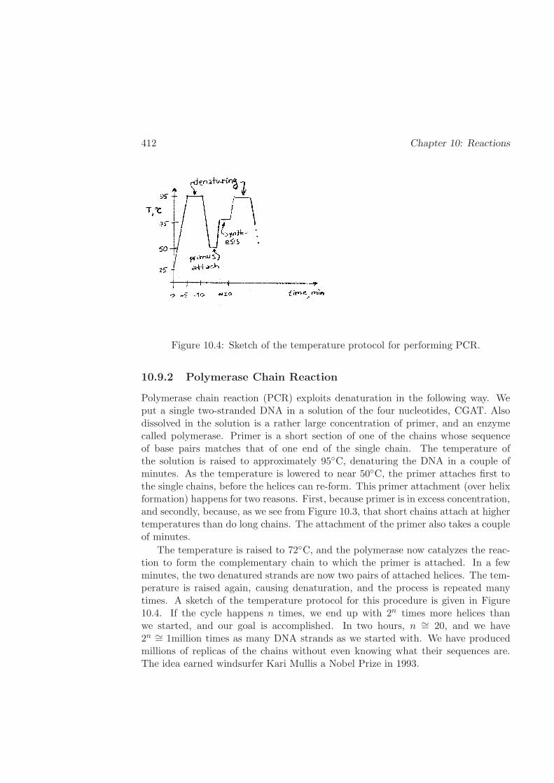
412 Chapter 10: Reactions
Figure 10.4: Sketch of the temperature protocol for performing PCR.
10.9.2 Polymerase Chain Reaction
Polymerase chain reaction (PCR) exploits denaturation in the following way. Weput a single two-stranded DNA in a solution of the four nucleotides, CGAT. Alsodissolved in the solution is a rather large concentration of primer, and an enzymecalled polymerase. Primer is a short section of one of the chains whose sequenceof base pairs matches that of one end of the single chain. The temperature ofthe solution is raised to approximately 95C, denaturing the DNA in a couple ofminutes. As the temperature is lowered to near 50C, the primer attaches first tothe single chains, before the helices can re-form. This primer attachment (over helixformation) happens for two reasons. First, because primer is in excess concentration,and secondly, because, as we see from Figure 10.3, that short chains attach at highertemperatures than do long chains. The attachment of the primer also takes a coupleof minutes.
The temperature is raised to 72C, and the polymerase now catalyzes the reac-tion to form the complementary chain to which the primer is attached. In a fewminutes, the two denatured strands are now two pairs of attached helices. The tem-perature is raised again, causing denaturation, and the process is repeated manytimes. A sketch of the temperature protocol for this procedure is given in Figure10.4. If the cycle happens n times, we end up with 2n times more helices thanwe started, and our goal is accomplished. In two hours, n ∼= 20, and we have2n ∼= 1million times as many DNA strands as we started with. We have producedmillions of replicas of the chains without even knowing what their sequences are.The idea earned windsurfer Kari Mullis a Nobel Prize in 1993.
May 5, 2010 413
There is an optimal range for choosing the length of the primer. If the primer istoo short, it might attach at several places along the chain, instead of just the end.If the primer is too long, it might take too long to attach.
10.10 Statistical Mechanics of Reactions and Denatu-ration
10.10.1 Stochastic Fluctuations in Reactions
Engineers are becoming increasingly interested in reactions in small volumes. Forexample, the reaction inside cells may involve only a few molecules of a large species;some reactors use small particles inside of which a small number of molecules arepolymerizing; and, some companies are forming “labs on a chip”, where smallamounts of quantities, like blood, are tested in tiny reactors created on silicon chips.In these situations, the traditional assumptions about large reactors no longer apply.Such is the case in small systems, similar to what we saw in §6.7.
On the one hand, the usual reaction rate equations as ordinary differential equa-tions, such as those learned in basic chemistry or reaction engineering, can be de-rived from molecular-level stochastic dynamical equations [103, Chapter IX]. Sucha derivation is beyond the scope of this text, so we will not consider it in detail.On the other hand, the same starting point applies to small systems; we considerreaction dynamics in general, large or small. The importance of fluctuations in reac-tions has recently been considered in the undergraduate chemical reactor textbookby Rawlings and Eckerdt [75, §4.8].
Stochastic Dynamics in a Linear, Reversible Reaction
We consider the simplest possible example to elucidate the technique, namely areversible, first-order reaction
Ak1k2
B. (10.61)
In this context, k1 is the probability that a single molecule of A reacts to form B,per unit time.
Imagine a box of volume V at temperature T , into which you place NA molecules
of A. After some period of time, there would be both A and B molecules such thatNA + NB = N
A. The number of such molecules NA would fluctuate with time;hence, there would be a probability p(NA; t) of having NA at time t. We can findthis probability through the idea of an ensemble of identical such boxes. If we had,

414 Chapter 10: Reactions
say millions of identical boxes, each in the state (T, V, NA), after some time, there
would be a distribution of mole numbers—each box would have its own NA. Thephysical definition of the probability, is that p(NA; t) is the fraction of boxes at timet with NA molecules of A, in the limit of infinitely many boxes.
The trick now is to focus on p(NA; t), instead of on an individual box. Thefraction of boxes with a given number of molecules changes because of the reactions.When a box with NA + 1 molecules of A forms a new molecule of B, then p(NA; t)must increase. The probability that one molecule reacts to form B is k1. There areNA + 1 such molecules, and fraction p(NA + 1; t) such boxes. Hence, we can write
∂p(NA; t)
∂t∼ k1(NA + 1)p(NA + 1; t). (10.62)
There are three other ways that the fraction of boxes with NA molecules can change:when a molecule of B reacts to form A, and the reverse of these two cases
∂p(NA; t)
∂t= k1
(
NA + 1)
p(NA + 1; t) + k2
(
NA − NA + 1
)
p(NA − 1; t)−
k1NAp(NA; t)− k2
(
NA − NA
)
p(NA; t). (10.63)
Note that we used the conservation of molecules to eliminate NB = NA − NA from
this expression. All the physical ideas are in this equation, and the rest is justmathematics, so make sure that you understand the origin of each term in theequation.
We know that large systems make only very small fluctuations around the aver-age number of molecules, 〈NA〉 :=
∑
NANAp(NA; t) (see §6.7). From Eqn. (10.63), it
is possible to construct an evolution equation for the average. This is accomplishedby multiplying with NA, and summing over all possible values for NA
∞∑
NA=0
NA∂p(NA; t)
∂t= k1
∞∑
NA=0
NA
(
NA + 1)
p(NA + 1; t) + (10.64)
k2
∞∑
NA=0
NA
(
NA − NA + 1
)
p(NA − 1; t) −
k1
∞∑
NA=0
N2Ap(NA; t)− k2
∞∑
NA=0
NA
(
NA − NA
)
p(NA; t).
To simplify this equation, we can pull the partial derivative out of the term on theleft side, and change the dummy summation variable in the first (NA → n− 1) and
May 5, 2010 415
second (NA → n + 1) terms on the right side. The third term on the right sideinvolves the average of the second moment. Hence, we obtain
∂
∂t
∞∑
NA=0
NAp(NA; t) = k1
∞∑
n=1
(n− 1)np(n; t) + k2
∞∑
n=0
(n+ 1)(NA − n)p(n; t)−
k1〈N2A〉 − k2
(
NA〈NA〉 − 〈N2
A〉)
.
d
dt〈NA〉 = k1
[
〈N2A〉 − 〈NA〉
]
+ k2
[
NA
(
〈NA〉+ 1)
+ 〈N2A〉 − 〈NA〉
]
−
k1〈N2A〉 − k2
(
NA〈NA〉 − 〈N2
A〉)
.
d
dt〈NA〉 = k2
(
NA − 〈NA〉
)
− k1〈NA〉. (10.65)
Note the simple final result. If we divide each side by the volume, we obtain anequation familiar from basic chemistry, or from reaction engineering
d
dtcA = −k1cA + k2(c
A − cA), (10.66)
where cA = 〈NA〉/V is the concentration of A (and the concentration of B is,from conservation again, cB = cA − cA). In other words, the probability evolutionequation, Eqn. (10.63), contains the simple reaction evolution equation with whichwe are familiar. However, it also contains more information, since we can also derivethe second moment evolution equation
d
dt〈N2
A〉 = k1
[
−2〈N2A〉+ 〈NA〉
]
+ k2
[
NA
(
2〈NA〉+ 1)
− 2〈N2A〉 − 〈NA〉
]
.
(10.67)
This equation is derived in a fashion very similar to that used to derive the evolutionequation for the average, Eqn. (10.65). Perhaps more useful is the evolution equationfor the variance, σ2N := 〈N2
A〉 − 〈NA〉2
d
dtσ2N = −2(k1 + k2)σ
2N + k1〈NA〉+ k2
[
NA − 〈NA〉
]
. (10.68)
The ODEs describing 〈NA〉 and σ2N , Eqs. (10.65) and (10.67) can be solved analyt-ically, since they are just linear ordinary differential equations
〈NA〉 = NA exp [−(k1 + k2)t] +
k2NA
k1 + k21− exp [−(k1 + k2)t] , (10.69)
σ2N =k1N
A
(k1 + k2)2k2 + (k1 − k2) exp [−(k1 + k2)t]− k1 exp [−2(k1 + k2)t] .
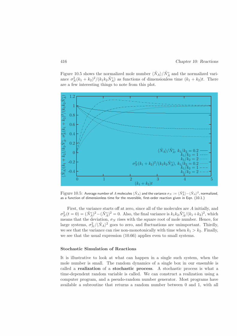
416 Chapter 10: Reactions
Figure 10.5 shows the normalized mole number 〈NA〉/NA and the normalized vari-
ance σ2N (k1 + k2)2/(k1k2N
A) as functions of dimensionless time (k1 + k2)t. There
are a few interesting things to note from this plot.
k1/k2 = 2k1/k2 = 1
σ2N(k1 + k2)
2/(k1k2NA), k1/k2 = 0.2
k1/k2 = 2k1/k2 = 1
〈NA〉/NA, k1/k2 = 0.2
(k1 + k2)t
〈NA〉(
k1+
k2)/
k2N
A,σ
2 N(k
1+
k2)2
/(k
1k
2N
A)
543210
1.2
1
0.8
0.6
0.4
0.2
0
-0.2
-0.4
Figure 10.5: Average number of Amolecules 〈NA〉 and the variance σN := 〈N2A〉−〈NA〉
2, normalized,as a function of dimensionless time for the reversible, first-order reaction given in Eqn. (10.1.)
First, the variance starts off at zero, since all of the molecules are A initially, andσ2N (t = 0) = (N
A)2−(N
A)2 = 0. Also, the final variance is k1k2N
A/(k1+k2)
2, whichmeans that the deviation, σN rises with the square root of mole number. Hence, forlarge systems, σ2N/〈NA〉2 goes to zero, and fluctuations are unimportant. Thirdly,we see that the variance can rise non-monotonically with time when k1 > k2. Finally,we see that the usual expression (10.66) applies even to small systems.
Stochastic Simulation of Reactions
It is illustrative to look at what can happen in a single such system, when themole number is small. The random dynamics of a single box in our ensemble iscalled a realization of a stochastic process. A stochastic process is what atime-dependent random variable is called. We can construct a realization using acomputer program, and a pseudo-random number generator. Most programs haveavailable a subroutine that returns a random number between 0 and 1, with all
May 5, 2010 417
numbers equally likely. Technically, this is called a uniform random number on thedomain zero to one. From our probability evolution equation, Eqn. (10.63), it ispossible to construct a computer algorithm.
The computer algorithm that we will construct here is not necessarily the mostefficient, but it is the simplest to understand, and sufficiently fast on even cheapand old computers, for our purposes. There is a second reason to construct suchan algorithm. Only for first-order reactions is it possible to find estimates for theaverages and variances analytically, in general. Van Kampen [103] has devised away to find the analytic evolution equations for the average and variance, but onlyin the limit of very large systems, and we are interested here in the behavior of smallsystems. More sophisticated algorithms may be found, for example, in [47].
To construct our algorithm, we integrate Eqn. (10.63) over a small time step ∆t.The term on the right side can be integrated analytically, using the fundamentaltheorem of calculus, §A.4. The terms on the right side, however, cannot be inte-grated analytically, since the probability function p depends on time. However, ifwe make our time-step size sufficiently small, we can approximate the integrand tobe nearly constant over the integral. Hence, we write
p(NA; t+∆t) ∼= p(NA; t) + k1
(
NA + 1)
p(NA + 1; t)∆t+
k2
(
NA − NA + 1
)
p(NA − 1; t)∆t−
k1NAp(NA; t)∆t− k2
(
NA − NA
)
p(NA; t)∆t. (10.70)
We use the algorithm in the following way. At the initial time t = 0, we begin withNA = N
A and NB = 0. Hence, we know the distribution function p: p(NA; t = 0) =
1, and all other p are zero. Then, Eqn. (10.70) becomes
p(NA; t = ∆t) = 1− k1N
A∆t
p(NA − 1; t = ∆t) = k1N
A∆t, (10.71)
and p(NA; t = ∆t) for all other values of NA are zero.
For this first time step, we use our pseudo-random number generator to give usX0 ∈ (0, 1). If X0 < k1N
A∆t, we set NA(t = ∆t) = N
A − 1; otherwise, we leave thenumber of moles of A unchanged.
For the second, and subsequent time steps, we use again Eqn. (10.70). At eachstep, we know the probability distribution from the results of our previous time step.Say that our previous time step n gave us the number of moles of A, NA(t = n∆t).Then, the algorithm gives us three possibilities for the next time step NA(t = (n+
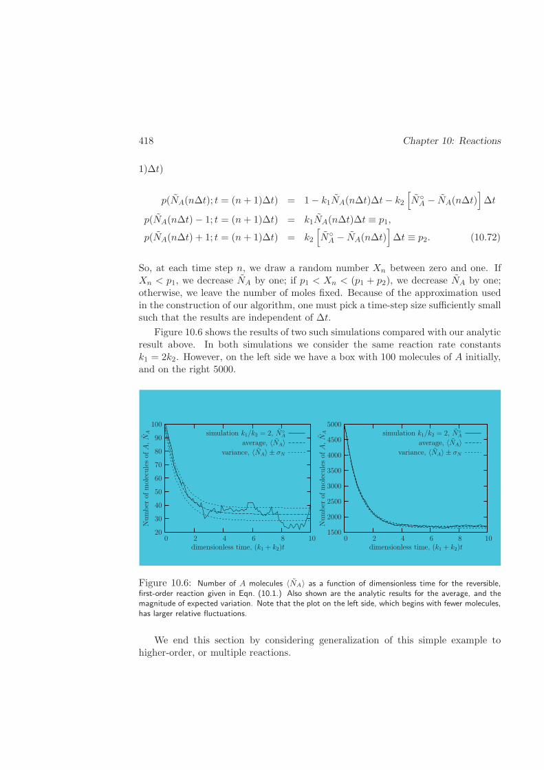
418 Chapter 10: Reactions
1)∆t)
p(NA(n∆t); t = (n+ 1)∆t) = 1− k1NA(n∆t)∆t− k2
[
NA − NA(n∆t)
]
∆t
p(NA(n∆t)− 1; t = (n+ 1)∆t) = k1NA(n∆t)∆t ≡ p1,
p(NA(n∆t) + 1; t = (n+ 1)∆t) = k2
[
NA − NA(n∆t)
]
∆t ≡ p2. (10.72)
So, at each time step n, we draw a random number Xn between zero and one. IfXn < p1, we decrease NA by one; if p1 < Xn < (p1 + p2), we decrease NA by one;otherwise, we leave the number of moles fixed. Because of the approximation usedin the construction of our algorithm, one must pick a time-step size sufficiently smallsuch that the results are independent of ∆t.
Figure 10.6 shows the results of two such simulations compared with our analyticresult above. In both simulations we consider the same reaction rate constantsk1 = 2k2. However, on the left side we have a box with 100 molecules of A initially,and on the right 5000.
variance, 〈NA〉 ± σN
average, 〈NA〉
simulation k1/k2 = 2, N
A
dimensionless time, (k1 + k2)t
Num
ber
ofm
olec
ule
sof
A,N
A
1086420
5000
4500
4000
3500
3000
2500
2000
1500
variance, 〈NA〉 ± σN
average, 〈NA〉
simulation k1/k2 = 2, N
A
dimensionless time, (k1 + k2)t
Num
ber
ofm
olec
ule
sof
A,N
A
1086420
100
90
80
70
60
50
40
30
20
Figure 10.6: Number of A molecules 〈NA〉 as a function of dimensionless time for the reversible,first-order reaction given in Eqn. (10.1.) Also shown are the analytic results for the average, and themagnitude of expected variation. Note that the plot on the left side, which begins with fewer molecules,has larger relative fluctuations.
We end this section by considering generalization of this simple example tohigher-order, or multiple reactions.
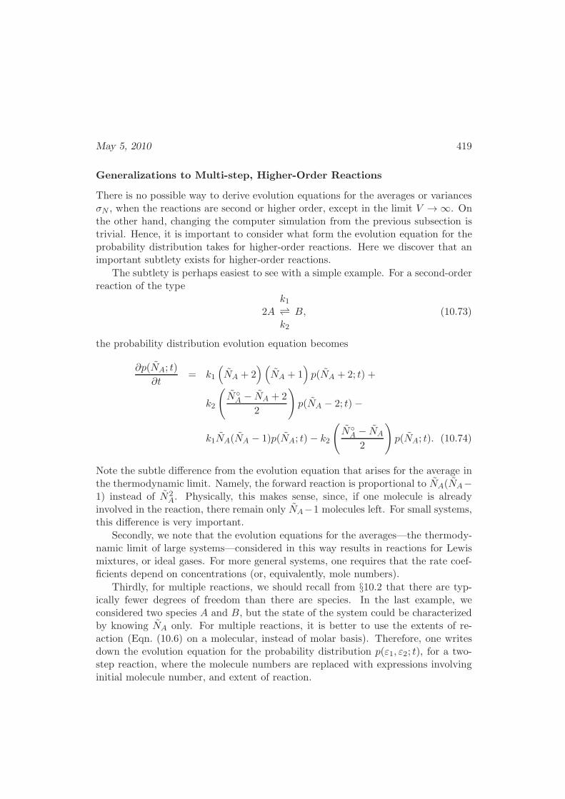
May 5, 2010 419
Generalizations to Multi-step, Higher-Order Reactions
There is no possible way to derive evolution equations for the averages or variancesσN , when the reactions are second or higher order, except in the limit V → ∞. Onthe other hand, changing the computer simulation from the previous subsection istrivial. Hence, it is important to consider what form the evolution equation for theprobability distribution takes for higher-order reactions. Here we discover that animportant subtlety exists for higher-order reactions.
The subtlety is perhaps easiest to see with a simple example. For a second-orderreaction of the type
2Ak1k2
B, (10.73)
the probability distribution evolution equation becomes
∂p(NA; t)
∂t= k1
(
NA + 2)(
NA + 1)
p(NA + 2; t) +
k2
(
NA − NA + 2
2
)
p(NA − 2; t)−
k1NA(NA − 1)p(NA; t)− k2
(
NA − NA
2
)
p(NA; t). (10.74)
Note the subtle difference from the evolution equation that arises for the average inthe thermodynamic limit. Namely, the forward reaction is proportional to NA(NA−1) instead of N2
A. Physically, this makes sense, since, if one molecule is alreadyinvolved in the reaction, there remain only NA−1 molecules left. For small systems,this difference is very important.
Secondly, we note that the evolution equations for the averages—the thermody-namic limit of large systems—considered in this way results in reactions for Lewismixtures, or ideal gases. For more general systems, one requires that the rate coef-ficients depend on concentrations (or, equivalently, mole numbers).
Thirdly, for multiple reactions, we should recall from §10.2 that there are typ-ically fewer degrees of freedom than there are species. In the last example, weconsidered two species A and B, but the state of the system could be characterizedby knowing NA only. For multiple reactions, it is better to use the extents of re-action (Eqn. (10.6) on a molecular, instead of molar basis). Therefore, one writesdown the evolution equation for the probability distribution p(ε1, ε2; t), for a two-step reaction, where the molecule numbers are replaced with expressions involvinginitial molecule number, and extent of reaction.
420 Chapter 10: Reactions
Figure 10.7: When an interior section of DNA has unbound base pairs, the structureis called a ‘bubble’.
Finally, we note that irreversible, multiple reactions can be fundamentally differ-ent, since extinction can occur. If one of your species in the reaction is a bacterium,for example, it is possible that all of the species die. At that point, the reactionscease. If one is considering the traditional average concentration, the possibility forextinction is ignored, and qualitatively different results for small and large systemscan be observed.
10.10.2 DNA Denaturation
We derive here the zipper model introduced in §10.9.1. We begin with a simplifiedpicture of the coil → helix transition for DNA. We assume
• All base pairs have the same free energy of binding ∆gbase.
• All bound pairs occupy adjacent sites on the chain—in other words, thereis only one continuous section of attached nucleotides on the chain, and no‘bubbles’ (see Figure 10.7).
• The free energy change associated with the first bound pair is much greaterthan that for the other pairs; this increase is primarily entropic, and thereforetemperature independent.
• The volume of the system is constant.
May 5, 2010 421
We picture two complementary chains of M nucleotides each. Adjacent basesdo not interact energetically to any significant extent. Since the adjacent base pairsare non-interacting, we can write the partition function as a product of individualbase pair partitions. We also need to sum up over all possible number of attachedpairs. Therefore, we write the chain partition function as
Q = qMu + qM−1u qfaωd(1) + qM−2
u qfaqaωd(2) + . . . , (10.75)
where qu(T ) is the partition function for an unattached pair, qfa(T ) is the partitionfunction for the first attached pair, qa(T ) is the partition function for each subse-quently attached pair, and ωd(N ) is the degeneracy, or number of ways that a chaincan have N attached base pairs. The first term on the right side is the contributionfrom two chains that are completely separated. The second term is for two chainsattached by a single base pair, and so on.
We assume that σ := qfa/qa, which is the extra entropic penalty for bringingthe two chains together, is temperature independent. This ratio is sometimes calledthe nucleation parameter. We expect the penalty to be large, so that σ ≪ 1.Putting this expression for σ into Eqn. (10.75) gives us
Q = qu(T )M + σ
M∑
N=1
ωd(N )qu(T )M−Nqa(T )
N . (10.76)
The degeneracy ωd(N) keeps track of the number of ways that a chain can haveN base pairs attached. Recall that these bound pairs are assumed to be adjacent.Hence, ωd = M − N + 1. We also define
qbase(T ) :=qa(T )
qu(T ), (10.77)
which, by its definition is exp(−∆gbase/kBT ), where ∆gbase is the change in freeenergy of a base pair upon attachment. Therefore, our partition function becomes
Q = qMu
1 + σ
M∑
N=1
(M − N + 1)qbase(T )N
(10.78)
= qMu
1 + σ
(M + 1)
M∑
N=1
qNbase −M∑
N=1
NqNbase
= qMu
1 + σ
[
(M + 1)− qbase∂
∂qbase
] M∑
N=1
qNbase
.
422 Chapter 10: Reactions
It is possible to find an algebraic expression for the sum in the following way
n∑
i=1
λi =
∞∑
i=0
λi − 1−∞∑
i=n+1
λi
=1
1− λ− 1− λn+1
∞∑
i=0
λi
=λ
1− λ− λn+1
1− λ
=λ(1− λn)
1− λ(10.79)
Hence, with a little more algebra, we obtain
Q = qMu
1 +
σqbase
[
M(1− qbase)− qbase(1− qMb )]
(1− qbase)2
. (10.80)
Recall that the free energy is −kBT times the logarithm of the partition function.We split up the free energy into that of the detached chains and the attached chainsof various amounts of helicity
F = Funattached +∆F helix. (10.81)
From our partition function, then, we have found the free energy for the unattachedchains
Funattached
kBT= −M log qu(T ), (10.82)
and the bound chains
∆F helix
kBT= − log
1 +
σqbase
[
M(1− qbase)− qbase(1− qMbase)]
(1− qbase)2
. (10.83)
The expression used in §10.9.1, namely Eqn. (10.57) replaces the Helmholtz potentialwith the Gibbs free energy as an approximation neglecting compressibility. Fromthe derivation, one can see the assumptions necessary to derive the expression.
From the first line of Eqn. (10.78), we see that the probability of having Nattached base pairs is
pN =σ(M − N + 1)qMu qbase(T )
N
Q(T, M). (10.84)
May 5, 2010 423
The average number of attached pairs can then be found using this probability asanother way to obtain Eqn. (10.60).
A somewhat more realistic model allows multiple sections of attached nucleotideson the chains. In other words, there can be a string of attached base pairs, thena string of detached base pairs, and then another string attached pairs, as shownin Figure 10.7. The resulting fundamental relation of the Zimm-Bragg MatrixModel is
∆F (T, M)
kBT= log
qbaseσ
(
1 + qbase +
√
(qbase − 1)2 + 4qbaseσ
)M+1
2M√
(qbase − 1)2 + 4qbaseσ
(
qbase − 1 +√
(qbase − 1)2 + 4qbaseσ
)
.
(10.85)
The derivation of this model is considered as an exercise. The functions showing uphere have the same meaning as those in the zipper model. We can expect these twomodels to give the same results when chains are not expected to have more thanone portion of the chain attached.
10.11 Summary
Upon completion of this chapter, the student should be able to
• Find the equilibrium composition for a reacting system, which we may writeas
0
r∑
i
νjiBi, j = 1, 2, . . . , q, (10.11′)
for r species and q reactions. In order to solve such problems, we found it usefulto introduce two new entities: the extent of reaction ε and the equilibriumconstant K. Since the total number of atoms are conserved in a reaction, thenumber of degrees of freedom is typically smaller than the number of moles ofall species present. Introducing the extent of reaction allows us to replace thenumber of moles Ni with ε, and the initial number of moles Ni,0
Ni = Ni,0 +
q∑
j=1
νji εj , i = 1, 2, . . . , r. (10.12′)
• Estimate the equilibrium constant K defined as
K(T ) := exp
(
−∆g
RT
)
, (10.21)
424 Chapter 10: Reactions
where the standard Gibbs free energy change of reaction is defined as
∆g(T ) :=r∑
i=1
νiµi . (10.22)
Here we use the chemical potential of the pure component at arbitrary T , butreference pressure P ref : µi := µpurei [P ref ].
• Find the equilibrium compositions from the expression
r∏
i=1
aνii = K(T ), equilibrium criterion, single reaction (10.20′)
where we use the activity defined by
ai :=fi(T, P, xi)fpurei (T, P ref)
, (10.19′)
when the equilibrium constant is already found. The activities are foundas functions of temperature, pressure, and composition using the techniquesintroduced in Chapters 8 and 9.
As examples, we considered the decomposition of silane used in chemical va-por deposition for producing silicon wafers (Example 10.6.2), production ofhydrogen from biomass, and DNA denaturation using a simple zipper model.Michaelis-Menten (or Monod) kinetics were also considered for two-step reac-tions.
• Estimate fluctuations in small reacting systems. We found a way to estimatethe size of the fluctuations analytically for first-order reactions, and showedhow to construct a simple computer algorithm for higher-order reactions.
• Derive simple statistical mechanical models for predicting the denaturation ofDNA.
May 5, 2010 425
10.12 Exercises
10.4.A. As part of the design of a smokestack scrubber, your engineering team willneed to estimate the importance of various reactions at many different temperatures.To aid in the design, make a plot of the equilibrium constant vs. temperature forthe reaction
SO2 +1
2O2 SO3, (10.86)
all of which are gases. Make sure that your data are valid in the range of your plot,and use 1 bar as your reference pressure.
10.4.B. Make a plot of the equilibrium constant vs. temperature for the reaction
CO +1
2O2 CO2, (10.87)
all of which are gases. Your temperature range should be 2000-4000K, and thereference pressure is 1 bar. In what temperature range is carbon dioxide favoredover carbon monoxide? What does this say about the catalytic converter in yourcar?
10.6.A. 3 It has been suggested that a new catalyst will be appropriate for use inthe manufacture of methanol and ethanol from synthesis gas, a mixture of carbonmonoxide and hydrogen. Consider the following reactions
CO + 2H2 CH3OH,
2CO + 4H2 C2H5OH +H2O. (10.88)
Determine the equilibrium composition which will be achieved at 400bar and 650Kwhen the initial mole ratio of hydrogen to carbon monoxide is 2. Use the enthalpyand Gibbs free energy of formation data from NIST. You may neglect the variationof the standard heat of reaction with temperature. Assume Lewis mixing, and usethe Peng-Robinson model to estimate the pure fugacity for each species.
10.6.B. One of your chemist colleagues at eRenewableEnergyTechLabs claims tohave developed a new catalyst to convert 95% pure ethane to ethylene and hydrogen
C2H6 C2H4 +H2 (10.89)
at 1000K and 1atm. Estimate the necessary pressure to obtain 95% conversion at1000K, and the necessary temperature to obtain the same conversion at 1atm. Isyour colleague correct?
3Problems A-E in this section are based on problems generously provided by Prof. Charles Hill,University of Wisconsin-Madison.
426 Chapter 10: Reactions
10.6.C. A mixture of carbon dioxide and hydrogen are flowing over a catalyst at1000K, and a pressure yet to be determined. Assuming that equilibrium is attained,you need to determine at what range of pressures carbon will be deposited on thecatalyst. You have good reason to believe that the following reactions are theimportant ones
C +H2O CO +H2,
C + 2H2O CO2 + 2H2,
CO2 + C 2CO,
CO +H2O CO2 +H2. (10.90)
At the given temperature, the reactions have equilibrium constants of 3.16, 5.01,2.00, and 1.58, respectively. The reference pressure is 1bar. Our inlet flow streamhas twice as many moles of hydrogen as carbon dioxide.
1. First, convince yourself that there are only two independent reactions.
2. Since we do not know the pressure yet, make the simplest possible assumptionfor all species: ideal gas. Now calculate the extent of reaction when no carbonis deposited (e.g., there is only one reaction). Find the exiting, equilibriumcomposition. Did we need to make any assumptions about the value for thepressure?
3. Now we consider what happens when carbon is deposited and one of the otherreactions comes into play. We wish to find the pressure where carbon is juststarting to deposit. Find this by taking the composition you just found andfind the pressure where one of the other equilibrium constants is satisfied.Assume unit activity for the solid carbon. This is the pressure where the firsttiny bit of carbon is deposited.
4. Now check your assumption for ideality at this pressure.
5. Finally, find the pressure necessary to convert half the incoming moles ofcarbon atoms to solid carbon, assuming ideality. Is this a good assumption?
10.6.D. Ethylbenzene is being synthesized from an equimolar mixture of ethyleneand benzene fed to a reactor at 400C and 2bar. All necessary thermodynamic dataare given in Table 10.2. You might find Eqn. (10.2) of the book useful.
Assuming that the reaction is isothermal and reaches equilibrium, find the exitingcomposition, and the amount of heat that must be removed per mole of feed.
Note that at this pressure ideality is probably a safe assumption.
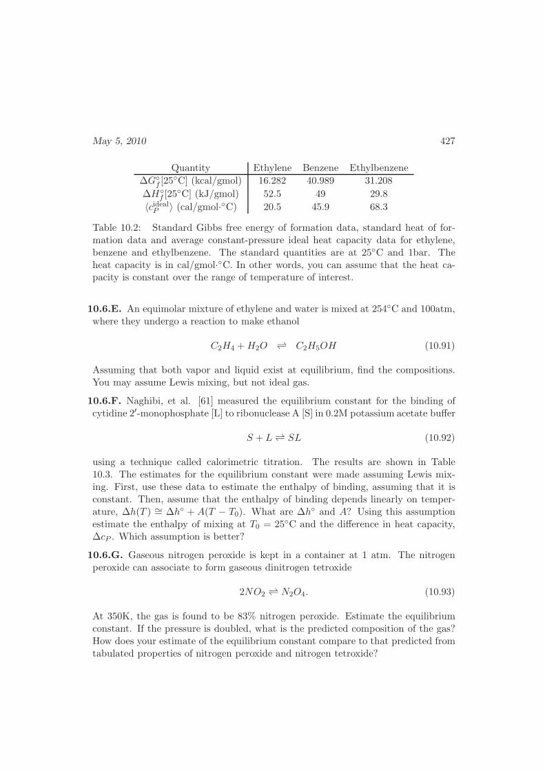
May 5, 2010 427
Quantity Ethylene Benzene Ethylbenzene
∆Gf [25
C] (kcal/gmol) 16.282 40.989 31.208
∆Hf [25
C] (kJ/gmol) 52.5 49 29.8
〈cidealP 〉 (cal/gmol·C) 20.5 45.9 68.3
Table 10.2: Standard Gibbs free energy of formation data, standard heat of for-mation data and average constant-pressure ideal heat capacity data for ethylene,benzene and ethylbenzene. The standard quantities are at 25C and 1bar. Theheat capacity is in cal/gmol·C. In other words, you can assume that the heat ca-pacity is constant over the range of temperature of interest.
10.6.E. An equimolar mixture of ethylene and water is mixed at 254C and 100atm,where they undergo a reaction to make ethanol
C2H4 +H2O C2H5OH (10.91)
Assuming that both vapor and liquid exist at equilibrium, find the compositions.You may assume Lewis mixing, but not ideal gas.
10.6.F. Naghibi, et al. [61] measured the equilibrium constant for the binding ofcytidine 2′-monophosphate [L] to ribonuclease A [S] in 0.2M potassium acetate buffer
S + L SL (10.92)
using a technique called calorimetric titration. The results are shown in Table10.3. The estimates for the equilibrium constant were made assuming Lewis mix-ing. First, use these data to estimate the enthalpy of binding, assuming that it isconstant. Then, assume that the enthalpy of binding depends linearly on temper-ature, ∆h(T ) ∼= ∆h + A(T − T0). What are ∆h and A? Using this assumptionestimate the enthalpy of mixing at T0 = 25C and the difference in heat capacity,∆cP . Which assumption is better?
10.6.G. Gaseous nitrogen peroxide is kept in a container at 1 atm. The nitrogenperoxide can associate to form gaseous dinitrogen tetroxide
2NO2 N2O4. (10.93)
At 350K, the gas is found to be 83% nitrogen peroxide. Estimate the equilibriumconstant. If the pressure is doubled, what is the predicted composition of the gas?How does your estimate of the equilibrium constant compare to that predicted fromtabulated properties of nitrogen peroxide and nitrogen tetroxide?
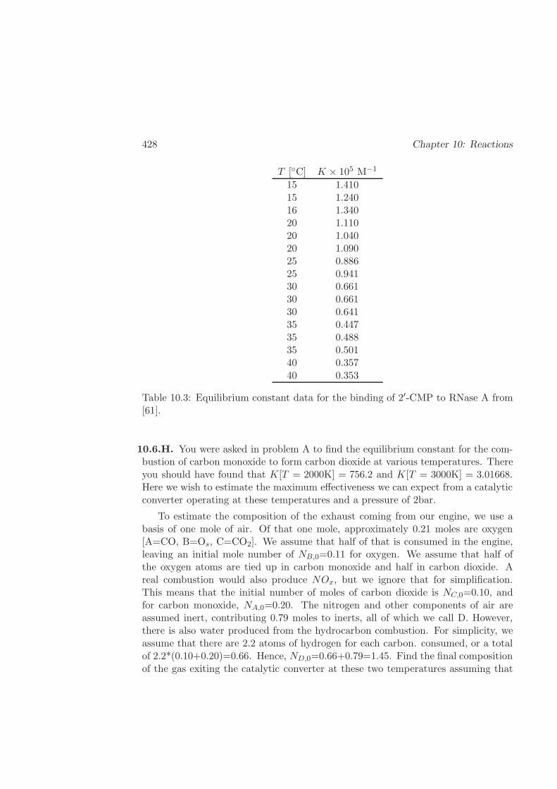
428 Chapter 10: Reactions
T [C] K × 105 M−1
15 1.41015 1.24016 1.34020 1.11020 1.04020 1.09025 0.88625 0.94130 0.66130 0.66130 0.64135 0.44735 0.48835 0.50140 0.35740 0.353
Table 10.3: Equilibrium constant data for the binding of 2′-CMP to RNase A from[61].
10.6.H. You were asked in problem A to find the equilibrium constant for the com-bustion of carbon monoxide to form carbon dioxide at various temperatures. Thereyou should have found that K[T = 2000K] = 756.2 and K[T = 3000K] = 3.01668.Here we wish to estimate the maximum effectiveness we can expect from a catalyticconverter operating at these temperatures and a pressure of 2bar.
To estimate the composition of the exhaust coming from our engine, we use abasis of one mole of air. Of that one mole, approximately 0.21 moles are oxygen[A=CO, B=Os, C=CO2]. We assume that half of that is consumed in the engine,leaving an initial mole number of NB,0=0.11 for oxygen. We assume that half ofthe oxygen atoms are tied up in carbon monoxide and half in carbon dioxide. Areal combustion would also produce NOx, but we ignore that for simplification.This means that the initial number of moles of carbon dioxide is NC,0=0.10, andfor carbon monoxide, NA,0=0.20. The nitrogen and other components of air areassumed inert, contributing 0.79 moles to inerts, all of which we call D. However,there is also water produced from the hydrocarbon combustion. For simplicity, weassume that there are 2.2 atoms of hydrogen for each carbon. consumed, or a totalof 2.2*(0.10+0.20)=0.66. Hence, ND,0=0.66+0.79=1.45. Find the final compositionof the gas exiting the catalytic converter at these two temperatures assuming that
May 5, 2010 429
equilibrium is reached.
10.6.I. Assuming the same initial compositions as problem H, find the final compo-sition of a mixture at 2000K and 1000bar. Note that it is unclear if we can assumean ideal gas at this pressure. However, we can assume Lewis mixing and use thePeng-Robinson model to estimate the pure fugacities.
10.8.A: An enzyme is rarely alone inside a cell. There also exist other species thatcan inhibit or activate a reaction catalyzed by an enzyme. Consider an enzyme Enin the presence of a single inhibitor I and a single activator A. The enzyme bindsto the substrate Su to produce product Pr, but can also form complexes with theinhibitor and activator
En+ SukfSukrSu
EnSukp−→ En+ Pr
En+AkfAkrA
EnA
EnA+ SukfASukrASu
EnSuAbkp−→ EnA+ Pr
En+ IkfIkrI
EnI
EnI + SukfISukrISu
EnSuIakp−→ EnI + Pr
EnSu+ IkfcIkrcI
EnSuI
EnSu+AkfcAkrcA
EnSuA (10.94)
Just as we did for Michaelis-Menten kinetics, assume here that all enzyme com-plexes, EnSu, EnSuA, and EnSuI reach a steady-state concentration. Further,ignore non-idealities so that concentration can be used. Find an expression for therate of production of dxPr
dt divided by the total enzyme concentration, xTE analo-gous to expression (10.56). In other words, your answer should be given only in
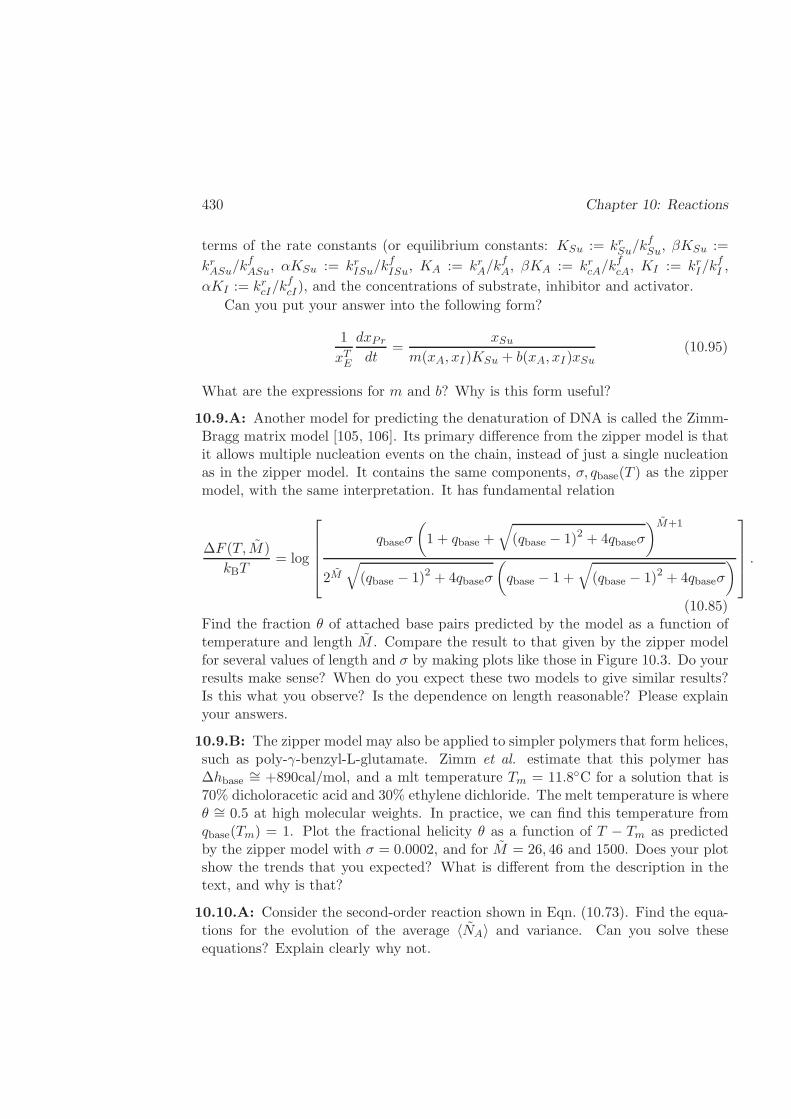
430 Chapter 10: Reactions
terms of the rate constants (or equilibrium constants: KSu := krSu/kfSu, βKSu :=
krASu/kfASu, αKSu := krISu/k
fISu, KA := krA/k
fA, βKA := krcA/k
fcA, KI := krI/k
fI ,
αKI := krcI/kfcI), and the concentrations of substrate, inhibitor and activator.
Can you put your answer into the following form?
1
xTE
dxPrdt
=xSu
m(xA, xI)KSu + b(xA, xI)xSu(10.95)
What are the expressions for m and b? Why is this form useful?
10.9.A: Another model for predicting the denaturation of DNA is called the Zimm-Bragg matrix model [105, 106]. Its primary difference from the zipper model is thatit allows multiple nucleation events on the chain, instead of just a single nucleationas in the zipper model. It contains the same components, σ, qbase(T ) as the zippermodel, with the same interpretation. It has fundamental relation
∆F (T, M )
kBT= log
qbaseσ
(
1 + qbase +√
(qbase − 1)2 + 4qbaseσ
)M+1
2M√
(qbase − 1)2 + 4qbaseσ
(
qbase − 1 +
√
(qbase − 1)2 + 4qbaseσ
)
.
(10.85)Find the fraction θ of attached base pairs predicted by the model as a function oftemperature and length M . Compare the result to that given by the zipper modelfor several values of length and σ by making plots like those in Figure 10.3. Do yourresults make sense? When do you expect these two models to give similar results?Is this what you observe? Is the dependence on length reasonable? Please explainyour answers.
10.9.B: The zipper model may also be applied to simpler polymers that form helices,such as poly-γ-benzyl-L-glutamate. Zimm et al. estimate that this polymer has∆hbase ∼= +890cal/mol, and a mlt temperature Tm = 11.8C for a solution that is70% dicholoracetic acid and 30% ethylene dichloride. The melt temperature is whereθ ∼= 0.5 at high molecular weights. In practice, we can find this temperature fromqbase(Tm) = 1. Plot the fractional helicity θ as a function of T − Tm as predictedby the zipper model with σ = 0.0002, and for M = 26, 46 and 1500. Does your plotshow the trends that you expected? What is different from the description in thetext, and why is that?
10.10.A: Consider the second-order reaction shown in Eqn. (10.73). Find the equa-tions for the evolution of the average 〈NA〉 and variance. Can you solve theseequations? Explain clearly why not.
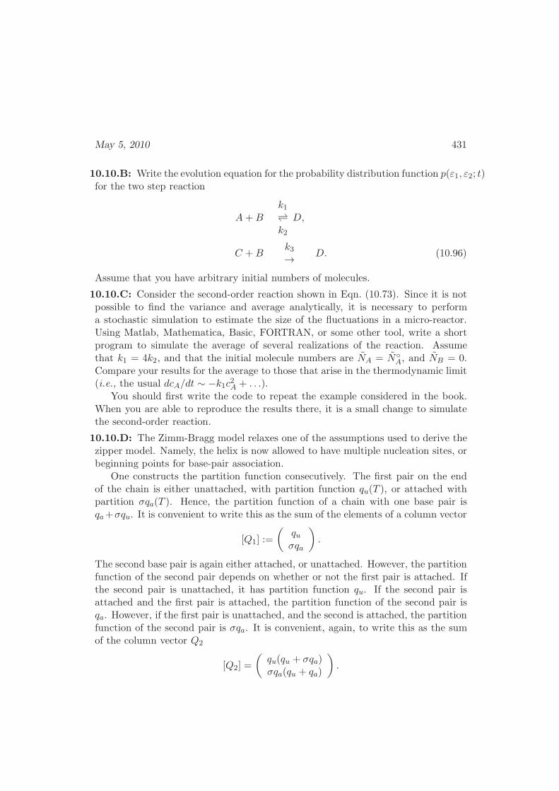
May 5, 2010 431
10.10.B: Write the evolution equation for the probability distribution function p(ε1, ε2; t)for the two step reaction
A+Bk1k2
D,
C +Bk3→ D. (10.96)
Assume that you have arbitrary initial numbers of molecules.
10.10.C: Consider the second-order reaction shown in Eqn. (10.73). Since it is notpossible to find the variance and average analytically, it is necessary to performa stochastic simulation to estimate the size of the fluctuations in a micro-reactor.Using Matlab, Mathematica, Basic, FORTRAN, or some other tool, write a shortprogram to simulate the average of several realizations of the reaction. Assumethat k1 = 4k2, and that the initial molecule numbers are NA = N
A, and NB = 0.Compare your results for the average to those that arise in the thermodynamic limit(i.e., the usual dcA/dt ∼ −k1c2A + . . .).
You should first write the code to repeat the example considered in the book.When you are able to reproduce the results there, it is a small change to simulatethe second-order reaction.
10.10.D: The Zimm-Bragg model relaxes one of the assumptions used to derive thezipper model. Namely, the helix is now allowed to have multiple nucleation sites, orbeginning points for base-pair association.
One constructs the partition function consecutively. The first pair on the endof the chain is either unattached, with partition function qu(T ), or attached withpartition σqa(T ). Hence, the partition function of a chain with one base pair isqa+σqu. It is convenient to write this as the sum of the elements of a column vector
[Q1] :=
(quσqa
)
.
The second base pair is again either attached, or unattached. However, the partitionfunction of the second pair depends on whether or not the first pair is attached. Ifthe second pair is unattached, it has partition function qu. If the second pair isattached and the first pair is attached, the partition function of the second pair isqa. However, if the first pair is unattached, and the second is attached, the partitionfunction of the second pair is σqa. It is convenient, again, to write this as the sumof the column vector Q2
[Q2] =
(qu(qu + σqa)σqa(qu + qa)
)
.
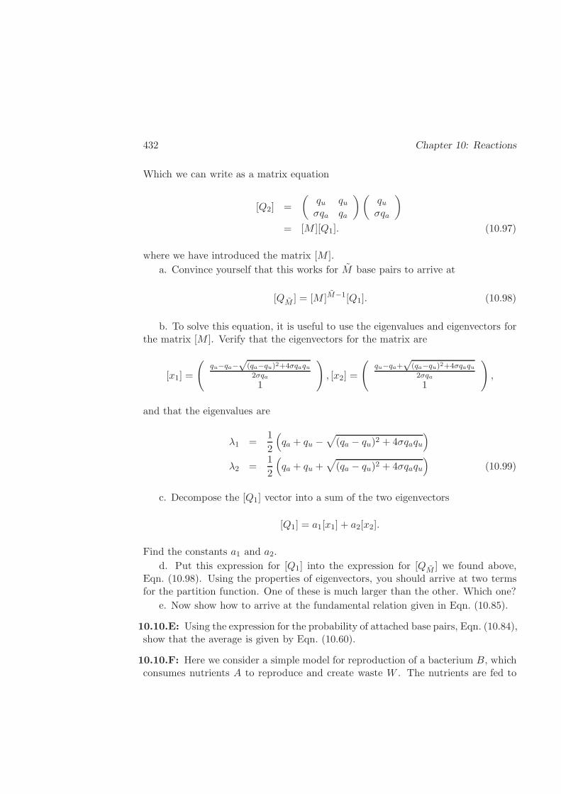
432 Chapter 10: Reactions
Which we can write as a matrix equation
[Q2] =
(qu quσqa qa
)(quσqa
)
= [M ][Q1]. (10.97)
where we have introduced the matrix [M ].
a. Convince yourself that this works for M base pairs to arrive at
[QM ] = [M ]M−1[Q1]. (10.98)
b. To solve this equation, it is useful to use the eigenvalues and eigenvectors forthe matrix [M ]. Verify that the eigenvectors for the matrix are
[x1] =
(qu−qa−
√(qa−qu)2+4σqaqu2σqa
1
)
, [x2] =
(qu−qa+
√(qa−qu)2+4σqaqu2σqa
1
)
,
and that the eigenvalues are
λ1 =1
2
(
qa + qu −√
(qa − qu)2 + 4σqaqu
)
λ2 =1
2
(
qa + qu +√
(qa − qu)2 + 4σqaqu
)
(10.99)
c. Decompose the [Q1] vector into a sum of the two eigenvectors
[Q1] = a1[x1] + a2[x2].
Find the constants a1 and a2.
d. Put this expression for [Q1] into the expression for [QM ] we found above,Eqn. (10.98). Using the properties of eigenvectors, you should arrive at two termsfor the partition function. One of these is much larger than the other. Which one?
e. Now show how to arrive at the fundamental relation given in Eqn. (10.85).
10.10.E: Using the expression for the probability of attached base pairs, Eqn. (10.84),show that the average is given by Eqn. (10.60).
10.10.F: Here we consider a simple model for reproduction of a bacterium B, whichconsumes nutrients A to reproduce and create waste W . The nutrients are fed to
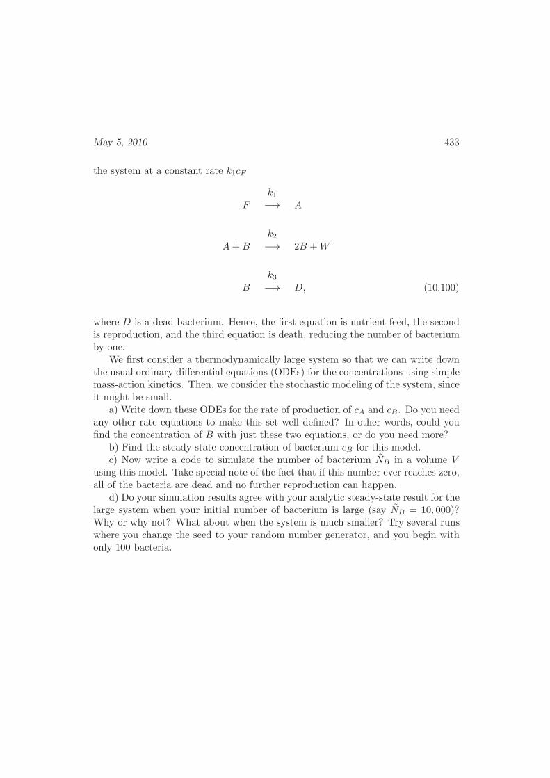
May 5, 2010 433
the system at a constant rate k1cF
Fk1−→ A
A+B
k2−→ 2B +W
Bk3−→ D, (10.100)
where D is a dead bacterium. Hence, the first equation is nutrient feed, the secondis reproduction, and the third equation is death, reducing the number of bacteriumby one.
We first consider a thermodynamically large system so that we can write downthe usual ordinary differential equations (ODEs) for the concentrations using simplemass-action kinetics. Then, we consider the stochastic modeling of the system, sinceit might be small.
a) Write down these ODEs for the rate of production of cA and cB . Do you needany other rate equations to make this set well defined? In other words, could youfind the concentration of B with just these two equations, or do you need more?
b) Find the steady-state concentration of bacterium cB for this model.c) Now write a code to simulate the number of bacterium NB in a volume V
using this model. Take special note of the fact that if this number ever reaches zero,all of the bacteria are dead and no further reproduction can happen.
d) Do your simulation results agree with your analytic steady-state result for thelarge system when your initial number of bacterium is large (say NB = 10, 000)?Why or why not? What about when the system is much smaller? Try several runswhere you change the seed to your random number generator, and you begin withonly 100 bacteria.

434 Chapter 10: Reactions
Chapter 11
Thermodynamics of Polymers
The word polymer comes from the latin polymeres, meaning many units. It isused to designate molecules with large molecular weights. There is no exact cutoffto determine when a large molecule is actually polymeric, but chained moleculesof molecular weight greater than a few thousand are typically considered to bepolymers.
Scientists and engineers are concerned with both naturally occurring and syn-thetic polymers. Naturally occurring polymers are important in biotechnologicaland biomedical fields, for example as DNA, RNA, microtubules, or actin filament,and in other fields, such as in the form of cellulosics in high-strength fibers.
Synthetic polymers play important roles in advanced materials such as plastics,liquid crystals, and fiber-reinforced composites. The manufacture of these materials,as well as numerous applications, often require that the polymer be dissolved insolvents, for example in spin-coating processes. Alternatively, material scientistsoften wish to combine the desirable properties of two different polymers in a plasticalloy by blending different mixtures of the two.
In this chapter, we consider the phase behavior of polymer solutions and themiscibility of polymer blends. The starting point for describing these properties isthe Flory-Huggins equation for the Gibbs free energy of mixing. In §11.1 we comparethe experimental data for the solubility of various polymer/solvent mixtures with theFlory-Huggins equation of state. We see that the theory is insufficient to describeall systems. Hence, in §11.2 we also consider generalizations to Flory-Huggins.
Finally, in §11.4 we derive the Flory-Huggins equation of state using the latticetheory introduced in §9.8.
435
436 Chapter 11: Thermodynamics of Polymers
11.1 Solubility and Miscibility of Polymer Solutions
In §8.6 we saw that assuming Lewis mixing rules leads to zero energy of mixing, andzero change in volume upon mixing. In §9.8.1 we saw how a statistical mechanicalmodel for binary mixtures of simple molecules that assumes constant volume and noheat of mixing leads to Lewis mixing. Hence, at first glance, we might be temptedto assume that a polymer solution that has no heat of mixing and constant volumewould also exhibit ideal mixing. However, the real behavior of polymer solutionsis much more complex. Much of the discrepancy between Lewis mixing and thebehavior of polymers can be attributed to the fact that polymers can stretch outand take many different conformations, and, hence, occupy much greater volumethan the solvent.
Therefore, the important parameters of description for a polymer solution are thevolume fraction of polymer, and the size of the polymer chain. The Flory-Hugginsmodel for binary mixtures of polymers predicts that the free energy of mixing isgiven by
∆gmix
RT=φArA
log φA +(1− φA)
rBlog(1− φA) + χ(T )φA(1− φA), (11.1)
where φA = NArA/(NArA + NBrB) is the volume fraction of species A, and rA isthe number of monomers (single units) that make up the polymer chain, calledthe degree of polymerization. We use the subscripts A and B to denote thetype of polymer when we are considering blends of polymers. If we are consideringa polymer solution, then B is a solvent so that rB ≡ rs = 1. The free energy ofmixing as given in Eqn. (11.1) is actually per mole of monomer , and not per moleof polymer. Hence, we multiply Eqn. (11.1) by (NArA +NBrB) to obtain
∆Gmix
RT= NA log φA +NB log (1− φA) + χ(T )NBφArB . (11.2)
The parameter χ(T ) is meant to describe the energy of interaction between thesolvent and the monomers. According to the theory of Flory and of Huggins, it maybe a function of temperature, but not of composition, and decreases with increasingtemperature.
If we plot the free energy of mixing for a polymer solution, with rA = 50, rB = 1and χ fifty percent larger than its critical value, as a function of mole fraction ofpolymer, Fig.(11.1) results. We see that the mixture is predicted to be globallyunstable over a range of volume fractions. Hence, the mixture should separate intoa polymer-rich phase x′′′′A and a polymer-poor phase x′A. These compositions arecalled binodal points, and the polymer mixture is always stable outside these points.
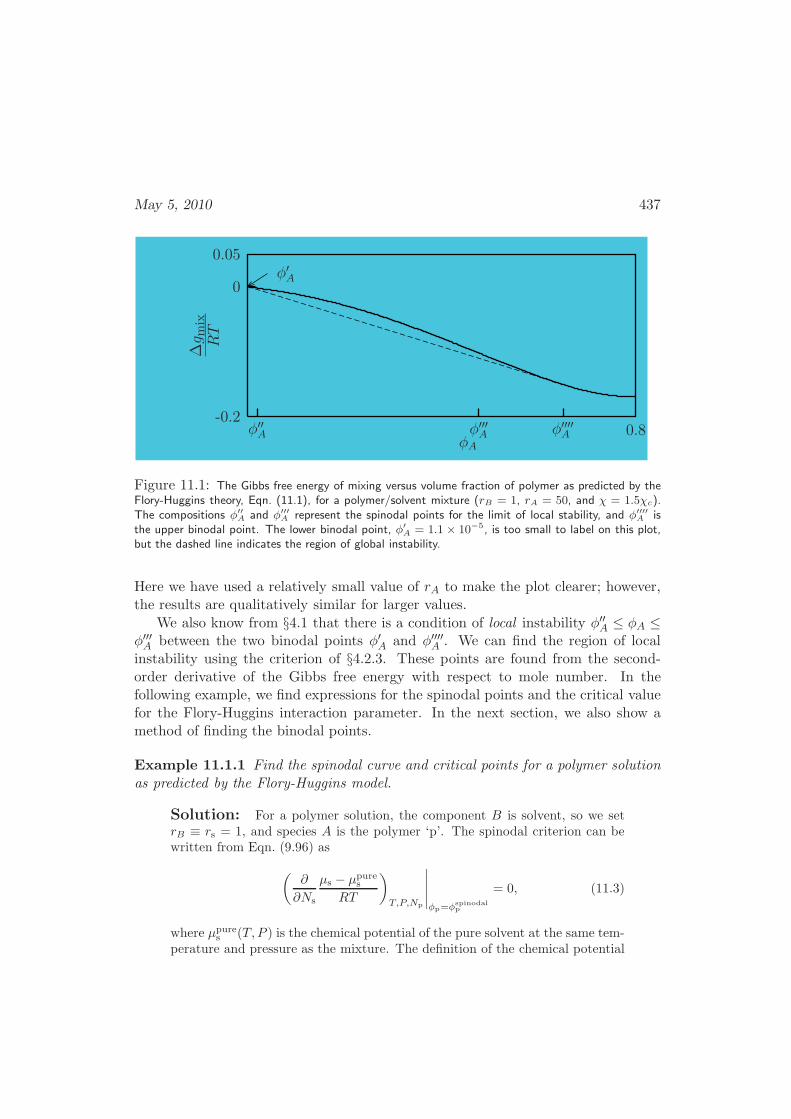
May 5, 2010 437
φ′
A
φA
∆gm
ix
RT
φ′′′′
Aφ′′′
Aφ′′
A 0.8
0.05
0
-0.2
Figure 11.1: The Gibbs free energy of mixing versus volume fraction of polymer as predicted by theFlory-Huggins theory, Eqn. (11.1), for a polymer/solvent mixture (rB = 1, rA = 50, and χ = 1.5χc).The compositions φ′′
A and φ′′′A represent the spinodal points for the limit of local stability, and φ′′′′
A isthe upper binodal point. The lower binodal point, φ′
A = 1.1 × 10⁻⁵, is too small to label on this plot,but the dashed line indicates the region of global instability.
Here we have used a relatively small value of rA to make the plot clearer; however,the results are qualitatively similar for larger values.
We also know from §4.1 that there is a condition of local instability φ′′A ≤ φA ≤φ′′′A between the two binodal points φ′A and φ′′′′A . We can find the region of localinstability using the criterion of §4.2.3. These points are found from the second-order derivative of the Gibbs free energy with respect to mole number. In thefollowing example, we find expressions for the spinodal points and the critical valuefor the Flory-Huggins interaction parameter. In the next section, we also show amethod of finding the binodal points.
Example 11.1.1 Find the spinodal curve and critical points for a polymer solutionas predicted by the Flory-Huggins model.
Solution: For a polymer solution, the component B is solvent, so we setrB ≡ rs = 1, and species A is the polymer ‘p’. The spinodal criterion can bewritten from Eqn. (9.96) as
(∂
∂Ns
µs − µpures
RT
)
T,P,Np
∣∣∣∣∣φp=φ
spinodalp
= 0, (11.3)
where µpures (T, P ) is the chemical potential of the pure solvent at the same tem-
perature and pressure as the mixture. The definition of the chemical potential
438 Chapter 11: Thermodynamics of Polymers
is
µs
RT:=
1
RT
(∂G
∂Ns
)
T,P,Np
=
(∂
∂Ns
∆Gmix +Nsµpures +Npµ
purep
RT
)
T,P,Np
=
(∂
∂Ns
∆Gmix
RT
)
T,P,Np
+µpures
RT, (11.4)
where the second line follows from the definition of a mixing property, Eqn. (9.101).Using the extensive form of the Flory-Huggins mixing law Eqn. (11.2), we find
µs − µpures
RT= log (1− φp) + φp
(
1− 1
rp
)
+ χφ2p, (11.5)
or similarly,
µp − µpurep
RT= logφp − (rp − 1) (1− φp) + χrp (1− φp)
2. (11.6)
We can now use this expression for the solvent chemical potential Eqn. (11.5)to find the spinodal points. However, since the expression is in terms of volumefraction, it is convenient to write
(∂
∂Ns
µs − µpures
RT
)
T,P,Np
=
(∂φp∂Ns
)
Np
(∂
∂φp
µs − µpures
RT
)
T,P,Np
= −φp(1 − φp)
Ns
(∂
∂φp
µs − µpures
RT
)
T,P,Np
Putting this result into Eqn. (11.3) implies the simpler (and general) spinodalcriterion
(∂
∂φp
µs − µpures
RT
)
T,P,Np
∣∣∣∣∣φp=φ
spinodalp
= 0. (11.7)
Using our expression for the solvent chemical potential, Eqn. (11.5), we find
(∂
∂φp
µs − µpures
RT
)
T,P,Np
∣∣∣∣∣φp=φ
spinodalp
= − 1
1− φspinodalp
+ 1− 1
rp+ 2χφspinodalp
0 = − 1
1− φspinodalp
+ 1− 1
rp+ 2χφspinodalp .
(11.8)
This quadratic equation can be solved for φspinodalp to find
φspinodalp =2χ− 1 + 1/rp ±
√(2χ− 1 + 1/rp)2 − 8χ/rp
4χ. (11.9)
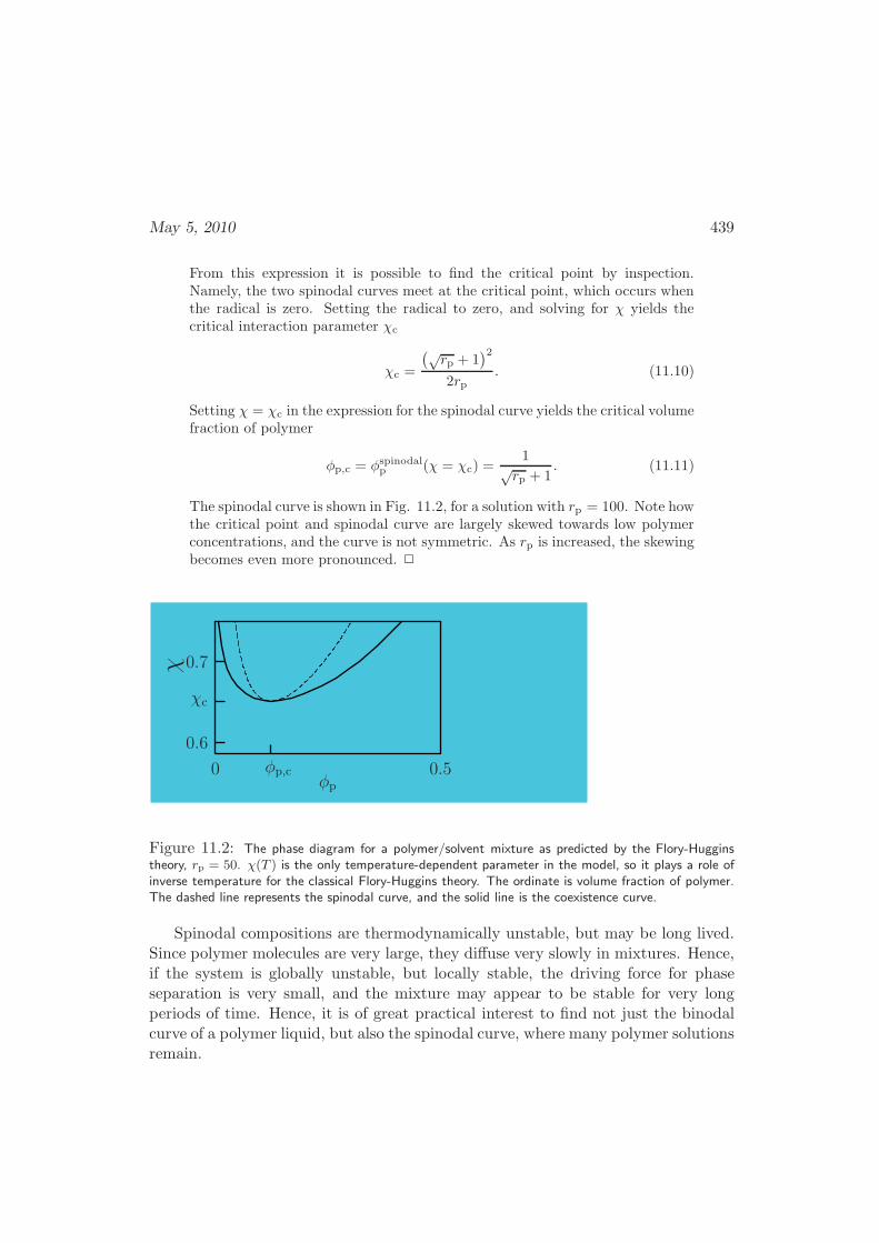
May 5, 2010 439
From this expression it is possible to find the critical point by inspection.Namely, the two spinodal curves meet at the critical point, which occurs whenthe radical is zero. Setting the radical to zero, and solving for χ yields thecritical interaction parameter χc
χc =
(√rp + 1
)2
2rp. (11.10)
Setting χ = χc in the expression for the spinodal curve yields the critical volumefraction of polymer
φp,c = φspinodalp (χ = χc) =1
√rp + 1
. (11.11)
The spinodal curve is shown in Fig. 11.2, for a solution with rp = 100. Note howthe critical point and spinodal curve are largely skewed towards low polymerconcentrations, and the curve is not symmetric. As rp is increased, the skewingbecomes even more pronounced. 2
φp
χ
φp,c 0.50
0.7
0.6
χc
Figure 11.2: The phase diagram for a polymer/solvent mixture as predicted by the Flory-Hugginstheory, rp = 50. χ(T ) is the only temperature-dependent parameter in the model, so it plays a role ofinverse temperature for the classical Flory-Huggins theory. The ordinate is volume fraction of polymer.The dashed line represents the spinodal curve, and the solid line is the coexistence curve.
Spinodal compositions are thermodynamically unstable, but may be long lived.Since polymer molecules are very large, they diffuse very slowly in mixtures. Hence,if the system is globally unstable, but locally stable, the driving force for phaseseparation is very small, and the mixture may appear to be stable for very longperiods of time. Hence, it is of great practical interest to find not just the binodalcurve of a polymer liquid, but also the spinodal curve, where many polymer solutionsremain.
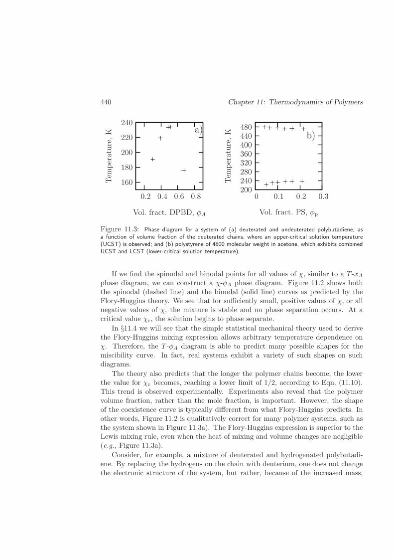
440 Chapter 11: Thermodynamics of Polymers
b)
Vol. fract. PS, φp
Tem
per
ature
,K
0 0.1 0.2 0.3
480440400360320280240200
a)
Vol. fract. DPBD, φA
Tem
per
ature
,K
0.2 0.4 0.6 0.8
240
220
200
180
160
Figure 11.3: Phase diagram for a system of (a) deuterated and undeuterated polybutadiene, asa function of volume fraction of the deuterated chains, where an upper-critical solution temperature(UCST) is observed; and (b) polystyrene of 4800 molecular weight in acetone, which exhibits combinedUCST and LCST (lower-critical solution temperature).
If we find the spinodal and binodal points for all values of χ, similar to a T -xAphase diagram, we can construct a χ-φA phase diagram. Figure 11.2 shows boththe spinodal (dashed line) and the binodal (solid line) curves as predicted by theFlory-Huggins theory. We see that for sufficiently small, positive values of χ, or allnegative values of χ, the mixture is stable and no phase separation occurs. At acritical value χc, the solution begins to phase separate.
In §11.4 we will see that the simple statistical mechanical theory used to derivethe Flory-Huggins mixing expression allows arbitrary temperature dependence onχ. Therefore, the T -φA diagram is able to predict many possible shapes for themiscibility curve. In fact, real systems exhibit a variety of such shapes on suchdiagrams.
The theory also predicts that the longer the polymer chains become, the lowerthe value for χc becomes, reaching a lower limit of 1/2, according to Eqn. (11.10).This trend is observed experimentally. Experiments also reveal that the polymervolume fraction, rather than the mole fraction, is important. However, the shapeof the coexistence curve is typically different from what Flory-Huggins predicts. Inother words, Figure 11.2 is qualitatively correct for many polymer systems, such asthe system shown in Figure 11.3a). The Flory-Huggins expression is superior to theLewis mixing rule, even when the heat of mixing and volume changes are negligible(e.g., Figure 11.3a).
Consider, for example, a mixture of deuterated and hydrogenated polybutadi-ene. By replacing the hydrogens on the chain with deuterium, one does not changethe electronic structure of the system, but rather, because of the increased mass,
May 5, 2010 441
changes the lengths of the bonds only slightly. Hence, from a chemical point ofview, the difference between the deuterated and undeuterated chains is nearly indis-tinguishable. So, at first it might seem surprising that such a system would phaseseparate at all.
However, the result can be predicted from Eqn. (11.1). Note that the first twoterms on the right side represent the entropy of mixing for the system. These termsare always negative, and hence are always stabilizing. The only source of instabilityis the energy of mixing, the third term on the right side of Eqn. (11.1). However,unlike the case for Lewis mixing, or the Margules equation, the stabilizing termsare weighted by the inverse of the degree of polymerization. Since the degree ofpolymerization is very large, these stabilizing terms are greatly diminished. Hence,very small energies of mixing can cause the system to phase separate. Consequently,mixing different chemical species can be extremely difficult for polymer blending.
On the other hand, many polymer systems exhibit much more complex phasebehavior. Figure 11.3b) shows the phase behavior of polystyrene in acetone whichexhibits two critical points: both an upper-critical solution temperature (UCST,the curve on bottom) and a lower-critical solution temperature (LCST, the curveon top). Systems that exhibit both UCST and LCST, at sufficiently high molecularweights, can exhibit an hourglass shape. The hourglass shape results from theconvergence of the UCST and LCST curves, resulting in no critical point.
Finally, Figure 11.5 on p.445 shows a solution that exhibits a closed-loop phasediagram. For this last example, there is an intermediate region of temperaturewhere the polymer solution phase separates. At both high and low temperatures,the polymer is fully soluble.
The Flory-Huggins theory as given by Eqn. (11.1) can explain all of this be-havior qualitatively if the interaction parameter is allowed to have non-monotonictemperature dependence. However, this generalization is not sufficient to describeexperimental data quantitatively . Thus, in the following section, we consider othermodels that are able to describe these more-complicated systems by allowing theinteraction parameter to depend on both temperature and composition.
11.2 Generalizations of the Flory-Huggins Theory
As we have seen in the last section, although it provides great insight into thethermodynamics of polymer solutions and blends, the Flory-Huggins theory has alimited capability of describing experimental data quantitatively. Also, the modelignores compressibility of polymer solutions. Here we consider three generalizationsto the Flory-Huggins theory. The first equation allows more quantitative predictionsof liquid-liquid equilibrium data, and the second allows compressibility. Third, a
442 Chapter 11: Thermodynamics of Polymers
model not considered in detail here, but widely used industrially is the PC-SAFTmodel derived from statistical mechanics [37].
11.2.1 Generalization of Qian, et al.
Qian, et al. [73] have considered an ad hoc modification to Eqn. (11.1) that is ableto predict all five types of phase behavior described in the last section: UCST,LCST, combined UCST and LCST, hourglass, and closed loop. By the addition ofadjustable parameters, the model is then able to describe more data quantitatively.
The free energy of mixing studied by Qian, et al. is
∆Gmix
RT= NA log φA +NB log(1 − φA) +NArAD(T )
∫ 1
φA
B(φ)dφ, (11.12)
Note that if we set B = 1, then we recover the Flory-Huggins expression with thefunction D(T ) playing the role of χ. We wish to have Flory-Huggins as a specialcase, so we consider the dependence
B(φ) = 1 + b1φ+ b2φ2. (11.13)
Then, the Flory-Huggins expression is recovered when b1 = b2 = 0.For the sake of simplicity, we focus on the shape of the spinodal curve predicted
by Eqn. (11.12), and recognize that the binodal curve must have a similar shape.Using the same procedure as that used in Example 11.1.1, we find the followingprediction for the solvent chemical potential
µB − µpureB
RT= log (1− φA) +
(rA − rBrA
)
φA +D(T )B(φA)rBφ2A. (11.14)
and for the other species
µA − µpureA
RT= log φA −
(rA − rBrB
)
(1− φA) +
rAD
[∫ 1
φA
B(φ)dφ−B(φA)φA(1− φA)
]
. (11.15)
The criterion for a spinodal point, Eqn. (11.7) becomes
0 =1
rA− 1
rB+
1
rB(1− φspinodalA )−D(T )C(φspinodalA ), (11.16)
where
C(φ) := 2B(φ) + φdB
dφ= 2 + 3b1φ+ 4b2φ
2. (11.17)
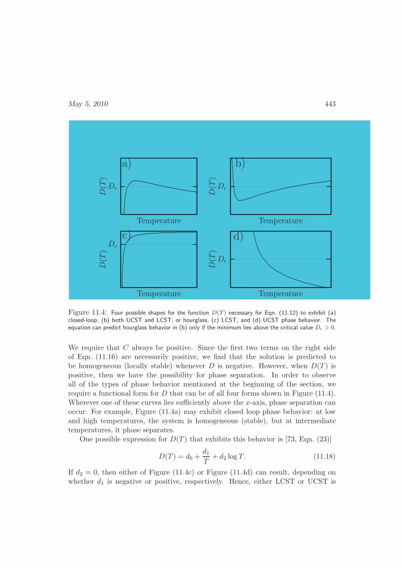
May 5, 2010 443
a)
Temperature
D(T
)
Dc
b)
TemperatureD
(T)
Dc
d)
Temperature
D(T
)
Dc
c)
Temperature
D(T
)
Dc
Figure 11.4: Four possible shapes for the function D(T ) necessary for Eqn. (11.12) to exhibit (a)closed-loop, (b) both UCST and LCST, or hourglass, (c) LCST, and (d) UCST phase behavior. Theequation can predict hourglass behavior in (b) only if the minimum lies above the critical value Dc > 0.
We require that C always be positive. Since the first two terms on the right sideof Eqn. (11.16) are necessarily positive, we find that the solution is predicted tobe homogeneous (locally stable) whenever D is negative. However, when D(T ) ispositive, then we have the possibility for phase separation. In order to observeall of the types of phase behavior mentioned at the beginning of the section, werequire a functional form for D that can be of all four forms shown in Figure (11.4).Wherever one of these curves lies sufficiently above the x-axis, phase separation canoccur. For example, Figure (11.4a) may exhibit closed loop phase behavior: at lowand high temperatures, the system is homogeneous (stable), but at intermediatetemperatures, it phase separates.
One possible expression for D(T ) that exhibits this behavior is [73, Eqn. (23)]
D(T ) = d0 +d1T
+ d2 log T. (11.18)
If d2 = 0, then either of Figure (11.4c) or Figure (11.4d) can result, depending onwhether d1 is negative or positive, respectively. Hence, either LCST or UCST is
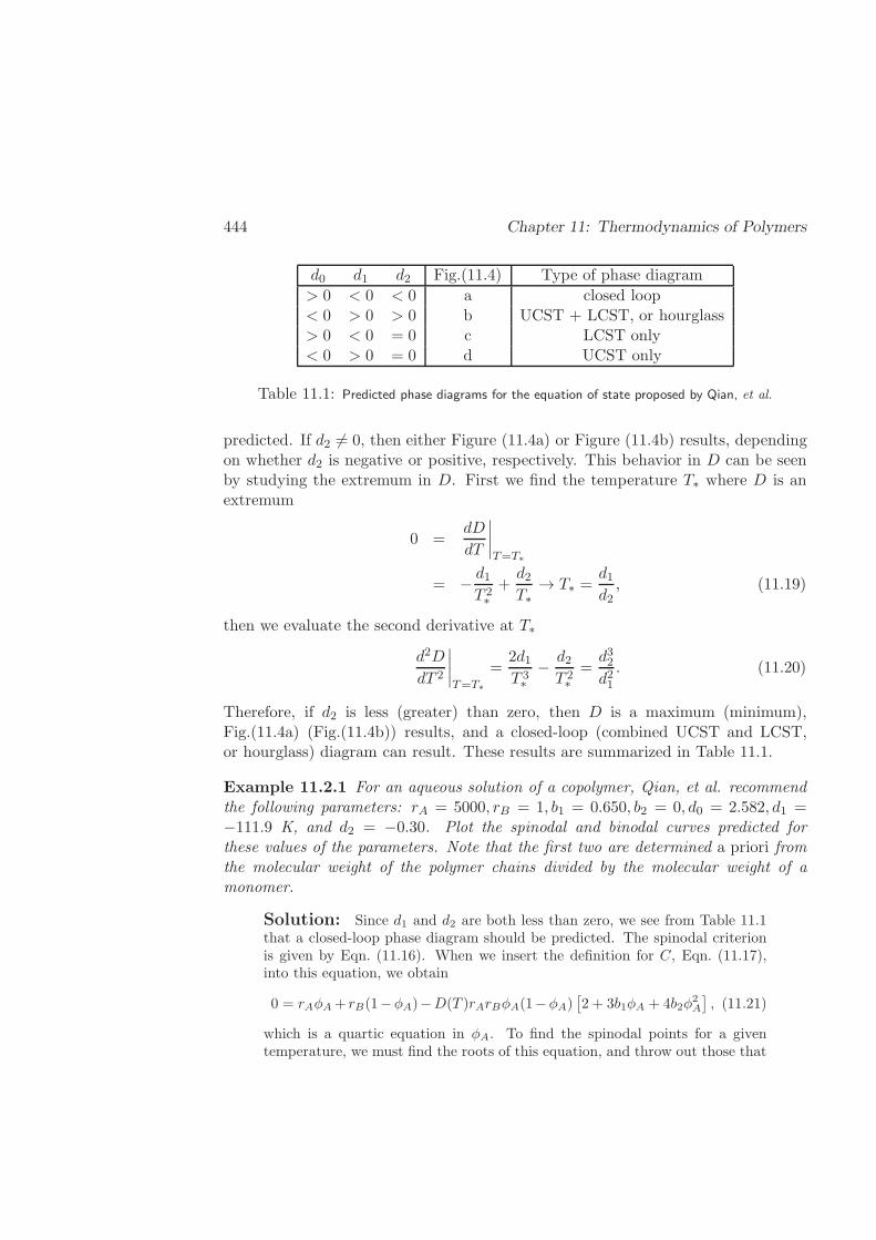
444 Chapter 11: Thermodynamics of Polymers
d0 d1 d2 Fig.(11.4) Type of phase diagram
> 0 < 0 < 0 a closed loop< 0 > 0 > 0 b UCST + LCST, or hourglass> 0 < 0 = 0 c LCST only< 0 > 0 = 0 d UCST only
Table 11.1: Predicted phase diagrams for the equation of state proposed by Qian, et al.
predicted. If d2 6= 0, then either Figure (11.4a) or Figure (11.4b) results, dependingon whether d2 is negative or positive, respectively. This behavior in D can be seenby studying the extremum in D. First we find the temperature T∗ where D is anextremum
0 =dD
dT
∣∣∣∣T=T∗
= − d1T 2∗
+d2T∗
→ T∗ =d1d2, (11.19)
then we evaluate the second derivative at T∗
d2D
dT 2
∣∣∣∣T=T∗
=2d1T 3∗
− d2T 2∗
=d32d21. (11.20)
Therefore, if d2 is less (greater) than zero, then D is a maximum (minimum),Fig.(11.4a) (Fig.(11.4b)) results, and a closed-loop (combined UCST and LCST,or hourglass) diagram can result. These results are summarized in Table 11.1.
Example 11.2.1 For an aqueous solution of a copolymer, Qian, et al. recommendthe following parameters: rA = 5000, rB = 1, b1 = 0.650, b2 = 0, d0 = 2.582, d1 =−111.9 K, and d2 = −0.30. Plot the spinodal and binodal curves predicted forthese values of the parameters. Note that the first two are determined a priori fromthe molecular weight of the polymer chains divided by the molecular weight of amonomer.
Solution: Since d1 and d2 are both less than zero, we see from Table 11.1that a closed-loop phase diagram should be predicted. The spinodal criterionis given by Eqn. (11.16). When we insert the definition for C, Eqn. (11.17),into this equation, we obtain
0 = rAφA+ rB(1−φA)−D(T )rArBφA(1−φA)[2 + 3b1φA + 4b2φ
2A
], (11.21)
which is a quartic equation in φA. To find the spinodal points for a giventemperature, we must find the roots of this equation, and throw out those that
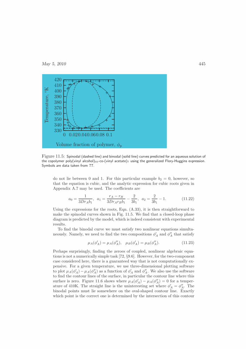
May 5, 2010 445
Volume fraction of polymer, φp
Tem
per
ature
,K
0.10.080.060.040.020
420410400390380370360350340330
Figure 11.5: Spinodal (dashed line) and binodal (solid line) curves predicted for an aqueous solution ofthe copolymer poly(vinyl alcohol)93-co-(vinyl acetate)7 using the generalized Flory-Huggins expression.Symbols are data taken from ??.
do not lie between 0 and 1. For this particular example b2 = 0, however, sothat the equation is cubic, and the analytic expression for cubic roots given inAppendix A.7 may be used. The coefficients are
a0 =1
3DrAb1, a1 =
rA − rB3DrArBb1
− 2
3b1, a2 =
2
3b1− 1. (11.22)
Using the expressions for the roots, Eqn. (A.33), it is then straightforward tomake the spinodal curves shown in Fig. 11.5. We find that a closed-loop phasediagram is predicted by the model, which is indeed consistent with experimentalresults.
To find the binodal curve we must satisfy two nonlinear equations simulta-neously. Namely, we need to find the two compositions φ′A and φ′′A that satisfy
µA(φ′A) = µA(φ
′′A), µB(φ
′A) = µB(φ
′′A). (11.23)
Perhaps surprisingly, finding the zeroes of coupled, nonlinear algebraic equa-tions is not a numerically simple task [72, §9.6]. However, for the two-componentcase considered here, there is a guaranteed way that is not computationally ex-pensive. For a given temperature, we use three-dimensional plotting softwareto plot µA(φ
′A)−µA(φ
′′A) as a function of φ′A and φ′′A. We also use the software
to find the contour lines of the surface, in particular the contour line where thissurface is zero. Figure 11.6 shows where µA(φ
′A) − µA(φ
′′A) = 0 for a temper-
ature of 410K. The straight line is the uninteresting set where φ′A = φ′′A. Thebinodal points must lie somewhere on the oval-shaped contour line. Exactlywhich point is the correct one is determined by the intersection of this contour
446 Chapter 11: Thermodynamics of Polymers
φ′
A
φ′′ A
0.10.080.060.040.020
0.1
0.08
0.06
0.04
0.02
0
Figure 11.6: Zeroes of µA(φ′A) − µA(φ
′′A) (solid lines) and µB(φ
′A) − µB(φ
′′A) (dashed lines) for a
temperature of 410K for the generalized Flory-Huggins model of Eqn. (11.12). The parameter valuesare given in Example 11.2.1. The binodal compositions are seen from this plot to be φ′
A = .0174 andφ′′A = 0.077.
line with the corresponding contour line for µB(φ′A) − µB(φ
′′A), also shown in
Fig. 11.6. Therefore, from this figure we find that at 410K, the binodal pointsare φ′A = 0.0174 and φ′′A = 0.077. If we go through this procedure for severalvalues of the temperature, we can construct the binodal curves shown in Fig-ure 11.5. The model shows good quantitative agreement with the data. Thesame curve can be found more quickly using Matlab, Mathematica, MathCAD,Octave, or similar software. 2
11.2.2 Sanchez-Lacombe Equation of State
The two polymer models considered so far for polymer liquids assume that they areincompressible. However, there are important industrial processes that exploit thecompressibility of polymers. Polymer foaming is an example.
Microcellular polymer foams (MPFs), are porous polymers generally character-ized by pore densities greater than 109 cells/cm3 and cell sizes smaller than 10microns. (See Figure 11.7). These novel polymeric materials have high strength-to-weight ratios and low densities, and are widely used in sports equipment, adsorbents,filters and catalyst supports. Microcellular foams are generated by initially saturat-
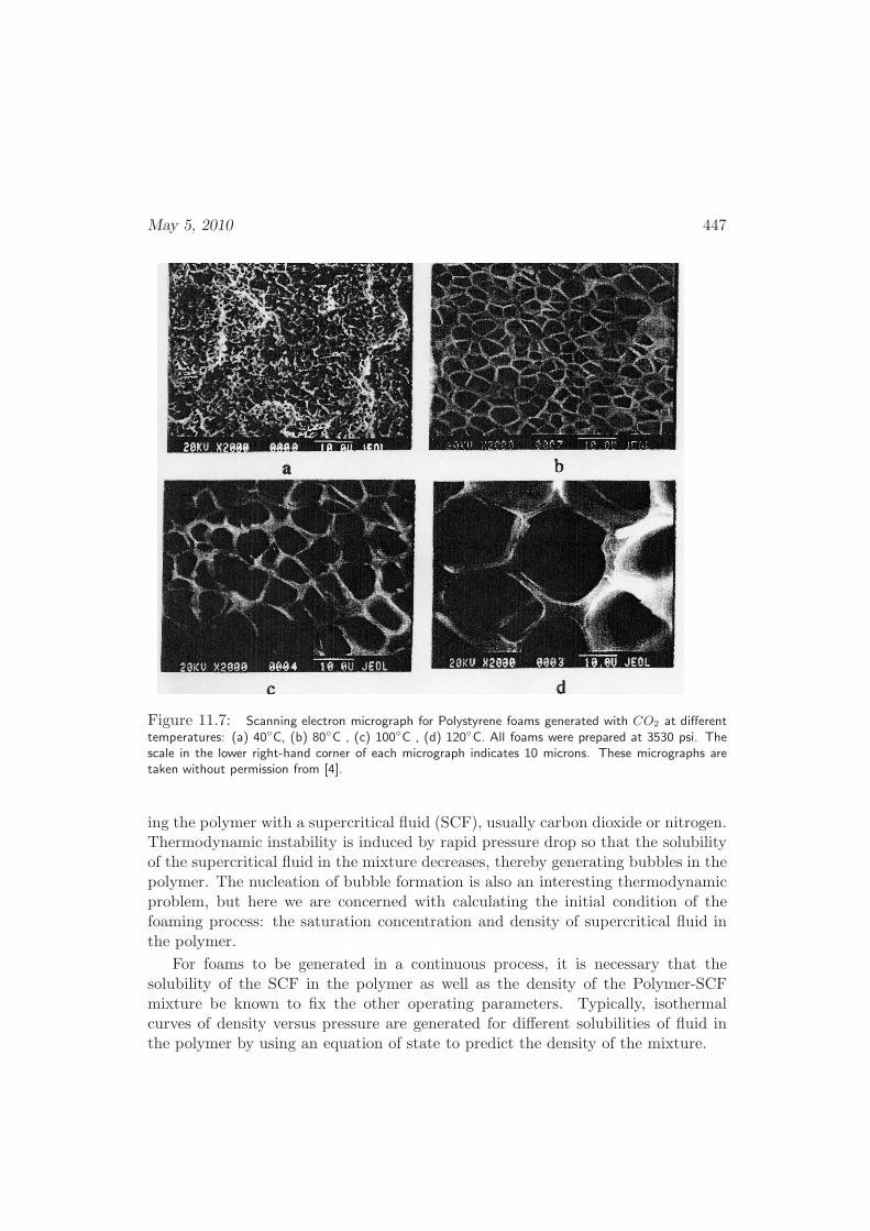
May 5, 2010 447
Figure 11.7: Scanning electron micrograph for Polystyrene foams generated with CO2 at differenttemperatures: (a) 40C, (b) 80C , (c) 100C , (d) 120C. All foams were prepared at 3530 psi. Thescale in the lower right-hand corner of each micrograph indicates 10 microns. These micrographs aretaken without permission from [4].
ing the polymer with a supercritical fluid (SCF), usually carbon dioxide or nitrogen.Thermodynamic instability is induced by rapid pressure drop so that the solubilityof the supercritical fluid in the mixture decreases, thereby generating bubbles in thepolymer. The nucleation of bubble formation is also an interesting thermodynamicproblem, but here we are concerned with calculating the initial condition of thefoaming process: the saturation concentration and density of supercritical fluid inthe polymer.
For foams to be generated in a continuous process, it is necessary that thesolubility of the SCF in the polymer as well as the density of the Polymer-SCFmixture be known to fix the other operating parameters. Typically, isothermalcurves of density versus pressure are generated for different solubilities of fluid inthe polymer by using an equation of state to predict the density of the mixture.
448 Chapter 11: Thermodynamics of Polymers
To model such a system one requires a fundamental relation that is applicableover a large range of densities. The Sanchez-Lacombe fundamental relation is onesuch PvT equation of state for polymers [55]. The model here is also lattice based,and has a generalization to the Flory-Huggins theory [81], where
G
rN= RT ∗
(P v
P ∗ − 1
v
)
+RT
[
(v − 1) log
(
1− 1
v
)
− 1
rlog v
]
. (11.24)
The reduced specific volume v is defined as
v :=P ∗vrRT ∗ . (11.25)
We have introduced characteristic pressure P ∗ and temperature T ∗. These arematerial parameters for either gas or polymer, and have been tabulated for manysubstances in Table 11.2. We have also introduced a dimensionless size parameterr, similar to that used in the Flory-Huggins theory. Usually tabulated is ρ∗, whichis related to r by
r =MwP
∗
RT ∗ρ∗. (11.26)
Recall that a fundamental relation for G requires independent parameters (T, P,N).However, Eqn. (11.24) also has the specific volume on the right side. In otherwords, the relation as it stands is over-specified. Sanchez and Lacombe completethe fundamental relation by finding an algebraic equation between v, T , P and N ,which fixes v. This equation is found by finding the v that minimizes the free energy.By setting the derivative of Eqn. (11.24) with respect to v equal to zero, we arriveat the additional equation of state
P
P ∗ = − 1
v2− T
T ∗
[
log
(
1− 1
v
)
+
(
1− 1
r
)1
v
]
, (11.27)
which determines v in Eqn. (11.24).Eqn. (11.24) is for pure-component species. The fundamental relation for a
gas/polymer mixture also requires mixing terms of the Flory-Huggins type, leadingto the fundamental relation
G
rN= RT ∗
(P v
P ∗ − 1
v
)
+RT
[
(v − 1) log
(
1− 1
v
)
− 1
rlog v
+φ1r1
log φ1 +φ2r2
log φ2
]
, (11.28)
where φi is the volume fraction of species i, and ri is its dimensionless volumeparameter. We also need a suitable mixing rule for the parameter values, analogous
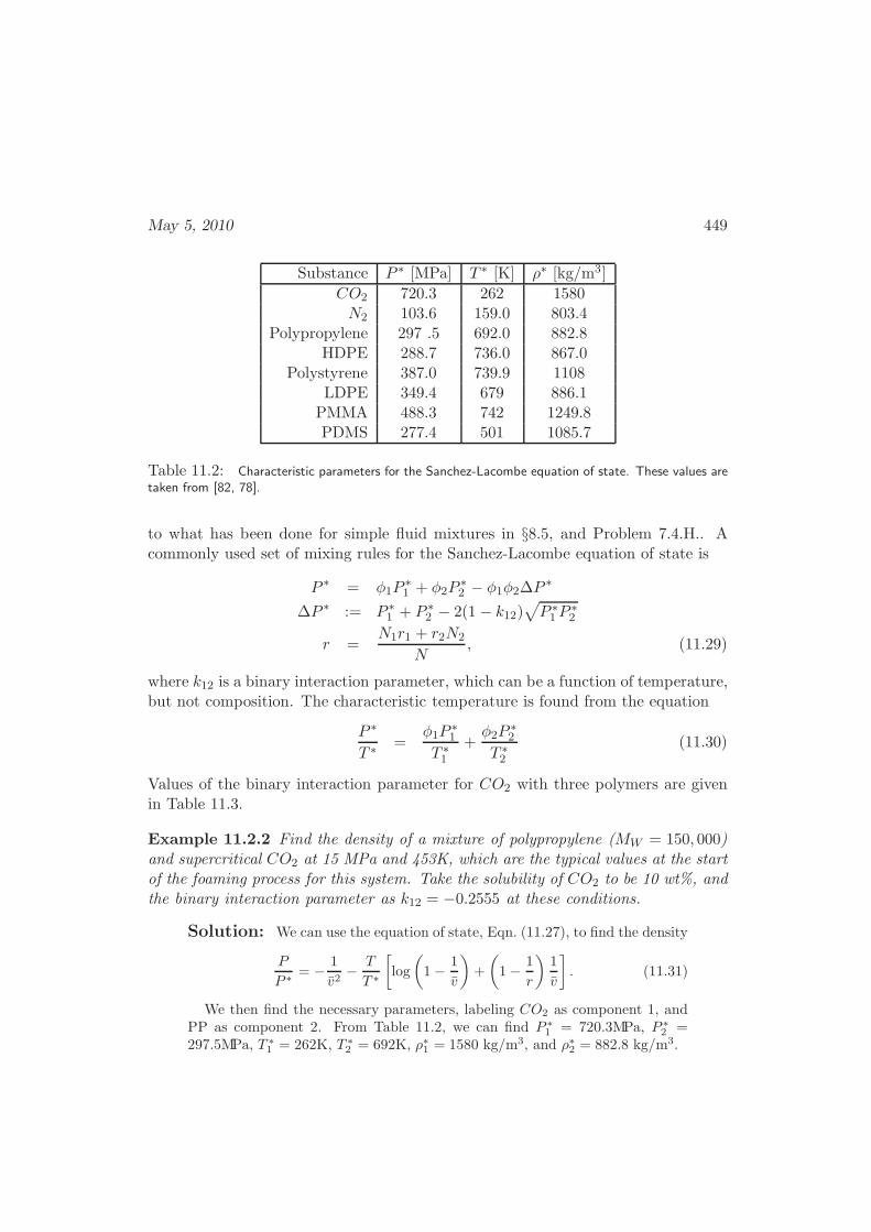
May 5, 2010 449
Substance P ∗ [MPa] T ∗ [K] ρ∗ [kg/m3]
CO2 720.3 262 1580N2 103.6 159.0 803.4
Polypropylene 297 .5 692.0 882.8HDPE 288.7 736.0 867.0
Polystyrene 387.0 739.9 1108LDPE 349.4 679 886.1
PMMA 488.3 742 1249.8PDMS 277.4 501 1085.7
Table 11.2: Characteristic parameters for the Sanchez-Lacombe equation of state. These values aretaken from [82, 78].
to what has been done for simple fluid mixtures in §8.5, and Problem 7.4.H.. Acommonly used set of mixing rules for the Sanchez-Lacombe equation of state is
P ∗ = φ1P∗1 + φ2P
∗2 − φ1φ2∆P
∗
∆P ∗ := P ∗1 + P ∗
2 − 2(1 − k12)√
P ∗1P
∗2
r =N1r1 + r2N2
N, (11.29)
where k12 is a binary interaction parameter, which can be a function of temperature,but not composition. The characteristic temperature is found from the equation
P ∗
T ∗ =φ1P
∗1
T ∗1
+φ2P
∗2
T ∗2
(11.30)
Values of the binary interaction parameter for CO2 with three polymers are givenin Table 11.3.
Example 11.2.2 Find the density of a mixture of polypropylene (MW = 150, 000)and supercritical CO2 at 15 MPa and 453K, which are the typical values at the startof the foaming process for this system. Take the solubility of CO2 to be 10 wt%, andthe binary interaction parameter as k12 = −0.2555 at these conditions.
Solution: We can use the equation of state, Eqn. (11.27), to find the density
P
P ∗= − 1
v2− T
T ∗
[
log
(
1− 1
v
)
+
(
1− 1
r
)1
v
]
. (11.31)
We then find the necessary parameters, labeling CO2 as component 1, andPP as component 2. From Table 11.2, we can find P ∗
1 = 720.3MPa, P ∗2 =
297.5MPa, T ∗1 = 262K, T ∗
2 = 692K, ρ∗1 = 1580 kg/m3, and ρ∗2 = 882.8 kg/m3.
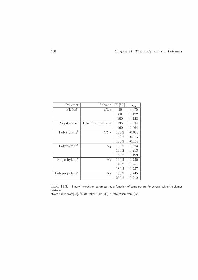
450 Chapter 11: Thermodynamics of Polymers
Polymer Solvent T [C] k12PDMSa CO2 50 0.075
80 0.122100 0.128
Polystyrenea 1,1-difluoroethane 135 0.034160 0.064
Polystyreneb CO2 100.2 -0.088140.2 -0.117180.2 -0.132
Polystyreneb N2 100.2 0.223140.2 0.213180.2 0.199
Polyethylenec N2 100.2 0.250140.2 0.251180.2 0.237
Polypropylenec N2 180.2 0.245200.2 0.212
Table 11.3: Binary interaction parameter as a function of temperature for several solvent/polymermixtures.aData taken from[35], bData taken from [83], cData taken from [82].
May 5, 2010 451
We convert from the given weight fraction to the volume fraction
φ1 =w1/ρ
∗1
w1/ρ∗1 + w2/ρ∗2
=0.10/1580kg/m
3
0.10/1580kg/m3 + 0.90/882.8kg/m3
= 0.0585, (11.32)
and, hence, φ2 = 0.9415. The dimensionless size parameters for each speciesare found using Eqn. (11.26)
r1 =MiP
∗i
RT ∗i ρ
∗i
=(44g/mol)(720.3MPa)
(8.314J/mol ·K)(1580kg/m3)(262K)
= 9.21, (11.33)
and r2 = 8786.17 by similar means. Hence, the dimensionless volume for themixture is
r =N1r1 +N2r2N1 +N2
=w1r1/M1 + w2r2/M2
w1/M1 + w2/M2
=(0.10)(9.21)/(44g/mol) + (0.90)(8786.17)/(150, 000g/mol)
(0.10)/(44g/mol) + (0.90)/(150, 000g/mol)
= 32.32, (11.34)
and the mixing rule for the size parameter yields r = 32.32. The contributionof mixing to P ∗ is
∆P ∗ := P ∗1 + P ∗
2 − 2(1− k12)√
P ∗1 P
∗2
= 720.3MPa+ 297.5MPa− 2(1 + 0.255)√
(720.3MPa)(297.5MPa)
= −144.6MPa. (11.35)
Therefore, the characteristic pressure for the mixture is
P ∗ = φ1P∗1 + φ2P
∗2 − φ1φ2∆P
∗
= (0.0585)(720.3MPa) + (0.9415)(297.5MPa) + (0.0585)(0.9415)(144.6MPa)
= 330.2MPa. (11.36)
452 Chapter 11: Thermodynamics of Polymers
Using the mixing rule for the characteristic temperature yields
T ∗ =P ∗
φ1P∗1
T∗1
+φ2P∗
2
T∗2
=(330.2MPa)
(0.0585)(720.3MPa)262K + (0.9415)(297.5MPa)
692K
= 584K. (11.37)
To obtain the last required parameter, we first need the molecular weight ofthe mixture, which is
Mw = x1M1 + x2M2
=w1
w1/M1 + w2/M2+
w2
w1/M1 + w2/M2
=0.10
0.10/(44g/mol) + 0.90/(150, 000g/mol)+
0.90
0.10/(44g/mol) + 0.90/(150, 000g/mol)
= 394.96g/mol. (11.38)
Then, we may finally find the characteristic density
ρ∗ =MwP
∗
RT ∗r
=(394.96g/mol)(330.2MPa)
(8.314MPa · cm3/mol ·K)(584.K)(32.32)
= 0.8311g/cm3. (11.39)
We may now find the necessary dimensionless thermodynamic variables
P
P ∗=
15MPa
330.2MPa= 0.04543
T
T ∗=
453K
584.K= 0.7759. (11.40)
The Sanchez-Lacombe equation of state, Eqn. (11.27) may be written in theform f(v) = 0, where
f(v) := P +1
v2+ T
[
log
(
1− 1
v
)
+
(
1− 1
r
)1
v
]
, (11.41)
= 0.04543 +1
v2+ (0.77595)
[
log
(
1− 1
v
)
+
(
1− 1
32.32
)1
v
]
.
In other words, the density is the root of the equation f(v) = 0. The root maybe found using Excel, Matlab, Mathematica, Maxima, FORTRAN, or many
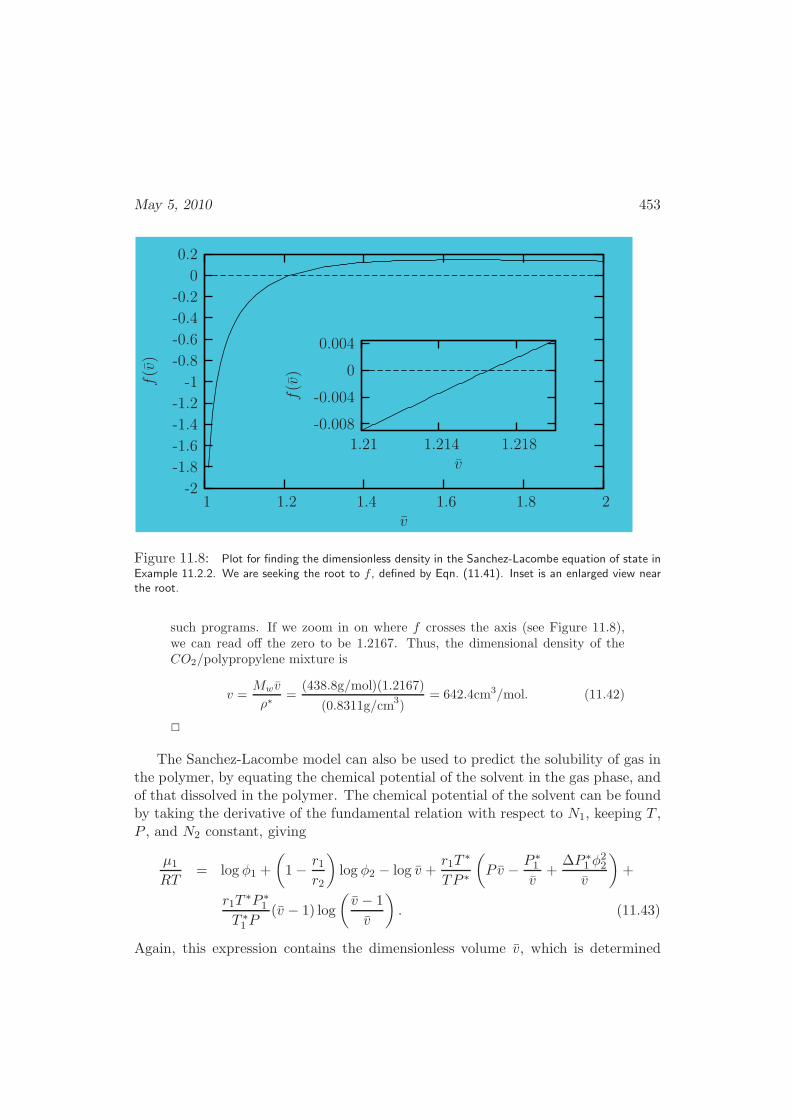
May 5, 2010 453
v
f(v
)
1.21 1.214 1.218
-0.008
-0.004
0
0.004
v
f(v
)
21.81.61.41.21
0.2
0
-0.2
-0.4
-0.6
-0.8
-1
-1.2
-1.4
-1.6
-1.8
-2
Figure 11.8: Plot for finding the dimensionless density in the Sanchez-Lacombe equation of state inExample 11.2.2. We are seeking the root to f , defined by Eqn. (11.41). Inset is an enlarged view nearthe root.
such programs. If we zoom in on where f crosses the axis (see Figure 11.8),we can read off the zero to be 1.2167. Thus, the dimensional density of theCO2/polypropylene mixture is
v =Mwv
ρ∗=
(438.8g/mol)(1.2167)
(0.8311g/cm3)
= 642.4cm3/mol. (11.42)
2
The Sanchez-Lacombe model can also be used to predict the solubility of gas inthe polymer, by equating the chemical potential of the solvent in the gas phase, andof that dissolved in the polymer. The chemical potential of the solvent can be foundby taking the derivative of the fundamental relation with respect to N1, keeping T ,P , and N2 constant, giving
µ1RT
= log φ1 +
(
1− r1r2
)
log φ2 − log v +r1T
∗
TP ∗
(
P v − P ∗1
v+
∆P ∗1 φ
22
v
)
+
r1T∗P ∗
1
T ∗1P
(v − 1) log
(v − 1
v
)
. (11.43)
Again, this expression contains the dimensionless volume v, which is determined
454 Chapter 11: Thermodynamics of Polymers
implicitly by Eqn. (11.27). Hence, two coupled, nonlinear equations must be solvedsimultaneously to obtain the solubility.
11.2.3 BGK Model
Another compressible model derived from statistical mechanics has been suggestedby Lipson and coworkers, and has the fundamental Helmholtz relation
F
RTNl=
r∑
i=0
φi
log φi +zl2log
[
γi∑q
j=0 γjφjqij(T )
]
. (11.44)
As before the volume fraction of species i is denoted by φi := riNiv/V . This speciesalso has a weighting parameter associated with it
γi := zl − 2 +2
ri, (11.45)
which is the average coordination number for each monomer of a chain with rimonomers. The monomer-monomer energetics give rise to a partition functionqij(T ), for interactions between a monomer of type i and one of type j. Typically,one assumes a single energy of interaction so that qij(T ) = exp (−ǫij/RT ).
The remaining parameter Nl is the number of lattice sites, which can be relatedto the volume, and the volume v of a lattice site
Nl :=V
v. (11.46)
Then we have parameters v, zl, ri, and the ǫij. To date zl is taken to always be6 in the model, and ri is the number of monomers in the chain.
What might seem strange about this expression is that there exists a speciesi = 0 in Eqn. (11.44). These terms represent empty sites on the lattice, allowing forcompressibility in the model. Therefore, φ0 = 1−∑q
i=1 φi.
What is particularly useful about this approach, is that most of the parameterscan be found strictly from compressibility data of the pure species. For example,the PV T equation of state for a single-component system can be found from themodel by setting q = 1 multiplying each side of Eqn. (11.44) by Nl, and taking thederivative with respect to volume to obtain
P v
RT= − log(1− φ1) +
zlγ21 [1− q11(T )]φ
21
2 [(γ1 − 1)φ1 + 1] [1− φ1 + γ1q(T )φ1]+zl2log [(γ1 − 1)φ1 + 1] .
(11.47)
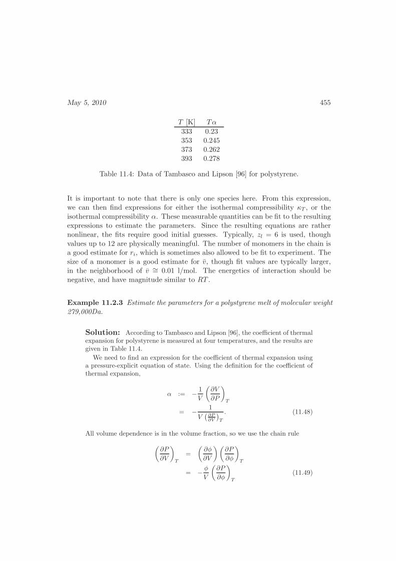
May 5, 2010 455
T [K] Tα
333 0.23353 0.245373 0.262393 0.278
Table 11.4: Data of Tambasco and Lipson [96] for polystyrene.
It is important to note that there is only one species here. From this expression,we can then find expressions for either the isothermal compressibility κT , or theisothermal compressibility α. These measurable quantities can be fit to the resultingexpressions to estimate the parameters. Since the resulting equations are rathernonlinear, the fits require good initial guesses. Typically, zl = 6 is used, thoughvalues up to 12 are physically meaningful. The number of monomers in the chain isa good estimate for ri, which is sometimes also allowed to be fit to experiment. Thesize of a monomer is a good estimate for v, though fit values are typically larger,in the neighborhood of v ∼= 0.01 l/mol. The energetics of interaction should benegative, and have magnitude similar to RT .
Example 11.2.3 Estimate the parameters for a polystyrene melt of molecular weight279,000Da.
Solution: According to Tambasco and Lipson [96], the coefficient of thermalexpansion for polystyrene is measured at four temperatures, and the results aregiven in Table 11.4.
We need to find an expression for the coefficient of thermal expansion usinga pressure-explicit equation of state. Using the definition for the coefficient ofthermal expansion,
α := − 1
V
(∂V
∂P
)
T
= − 1
V(∂P∂V
)
T
. (11.48)
All volume dependence is in the volume fraction, so we use the chain rule
(∂P
∂V
)
T
=
(∂φ
∂V
)(∂P
∂φ
)
T
= − φ
V
(∂P
∂φ
)
T
(11.49)
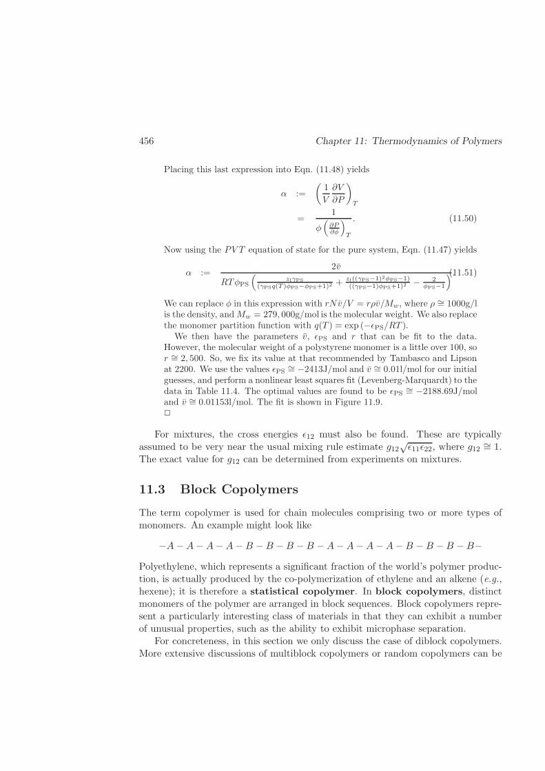
456 Chapter 11: Thermodynamics of Polymers
Placing this last expression into Eqn. (11.48) yields
α :=
(1
V
∂V
∂P
)
T
=1
φ(∂P∂φ
)
T
. (11.50)
Now using the PV T equation of state for the pure system, Eqn. (11.47) yields
α :=2v
RTφPS
(zlγPS
(γPSq(T )φPS−φPS+1)2 + zl((γPS−1)2φPS−1)((γPS−1)φPS+1)2 − 2
φPS−1
) .(11.51)
We can replace φ in this expression with rNv/V = rρv/Mw, where ρ ∼= 1000g/lis the density, andMw = 279, 000g/mol is the molecular weight. We also replacethe monomer partition function with q(T ) = exp (−ǫPS/RT ).
We then have the parameters v, ǫPS and r that can be fit to the data.However, the molecular weight of a polystyrene monomer is a little over 100, sor ∼= 2, 500. So, we fix its value at that recommended by Tambasco and Lipsonat 2200. We use the values ǫPS
∼= −2413J/mol and v ∼= 0.01l/mol for our initialguesses, and perform a nonlinear least squares fit (Levenberg-Marquardt) to thedata in Table 11.4. The optimal values are found to be ǫPS
∼= −2188.69J/moland v ∼= 0.01153l/mol. The fit is shown in Figure 11.9.2
For mixtures, the cross energies ǫ12 must also be found. These are typicallyassumed to be very near the usual mixing rule estimate g12
√ǫ11ǫ22, where g12 ∼= 1.
The exact value for g12 can be determined from experiments on mixtures.
11.3 Block Copolymers
The term copolymer is used for chain molecules comprising two or more types ofmonomers. An example might look like
−A−A−A−A−B −B −B −B −A−A−A−A−B −B −B −B−
Polyethylene, which represents a significant fraction of the world’s polymer produc-tion, is actually produced by the co-polymerization of ethylene and an alkene (e.g.,hexene); it is therefore a statistical copolymer. In block copolymers, distinctmonomers of the polymer are arranged in block sequences. Block copolymers repre-sent a particularly interesting class of materials in that they can exhibit a numberof unusual properties, such as the ability to exhibit microphase separation.
For concreteness, in this section we only discuss the case of diblock copolymers.More extensive discussions of multiblock copolymers or random copolymers can be
May 5, 2010 457
340 350 360 370 380 390T @KD
0.23
0.24
0.25
0.26
0.27
TΑ
Figure 11.9: Dimensionless coefficient of thermal expansion as a function of tem-perature for a polystyrene liquid. The symbols are data taken from Tambasco andLipson [96], and the curve is the fit to Eqn. (11.51). The parameter values are givenin the text.
found in the specialized literature. Consider a diblock copolymer of monomers Aand B. The block co-polymer shown above provides a schematic representation ofa symmetric diblock copolymer; one in which the degree of polymerization isthe same for both blocks. If fA is used to denote the fraction of A monomers ina molecule, then for a symmetric diblock copolymer fA = fB = 1
2 . If the twomonomers were similar, one would expect the behavior of the diblock copolymerto be analogous to that of regular homopolymers. However, in situations wherethe two monomers are fairly different, one would expect the two blocks to becomeimmiscible. That is indeed what is observed in experiments: below a certain criticaltemperature, the two blocks of a diblock copolymer phase separate but, given thatthey’re “joined at the hip”, the two blocks cannot go too far from each other.This leads to the formation of microdomains of A and B segments, or microphaseseparation.
Depending on the composition of the molecule (i.e., the value of fA), a diblockcopolymer can form a variety of ordered microphases. Figure 11.10 provides aschematic representation of the microphases observed in typical diblock copolymers;
458 Chapter 11: Thermodynamics of Polymers
these include spherical domains, cylinders, and lamellae. Figure 11.10 shows thephase diagram for a polystyrene-poly(2-vinylpyridine) diblock copolymer. For smallvalues of fA the system forms spheres of one block dispersed in a matrix of the otherblock, for slightly larger values of fA the system prefers to form cylinders, and forsymmetric molecules the material forms lamellae.
In order to understand the nature of microphase separation in block copolymers,it is useful to construct a simple phenomenological theory that is based on ideaspresented earlier in this text. For simplicity, we restrict our discussion to the caseof symmetric molecules. To construct such a model, we begin by enumerating thevarious contributions that one would expect to the free energy:
• Chain stretching: in a lamellar phase, polymer molecules are stacked on eachother in a parallel fashion; the A and B blocks repel each other, leading to theformation of distinct lamellar domains. This microphase separated state canonly be achieved by stretching the molecules. The corresponding free energycan therefore be written as
FsRT
=3
8NKa2KL2 (11.52)
where L is the thickness (or period) of the lamellar microdomains, NK is thenumber of segments and aK is the so-called Kuhn length of the segments.The Kuhn length represents a characteristic length beyond which groups ofmonomers along the molecule can be assumed to be independent of each other.For a typical polymer, the Kuhn length comprises on the order of 5 to 20monomers, the precise number depending on the chemical constitution of themolecule [29, 32, 31]. This expression is an approximation to the inverseLangevin expression, valid for small extensions of the strand, first seen inExercise 3.7.B. The statistical mechanical derivation of that expression wasshown in §6.6. Exercise 6.6.D deals with the derivation of this expression.
• Interfacial free energy: the segregation of the molecules into highly organizedlamella involves the formation of an interface between the A and B blocks.This interface has a free energy of the form
FγRT
=AchainγAB
RT(11.53)
where γAB is the interfacial tension between blocks A and B, and where Achain
is used to denote the interfacial area per chain. This expression is covered ingreater detail in the following chapter.
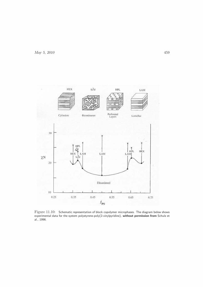
May 5, 2010 459
Figure 11.10: Schematic representation of block copolymer microphases. The diagram below showsexperimental data for the system polystyrene-poly(2-vinylpyridine), without permission from Schulz etal., 1996.
460 Chapter 11: Thermodynamics of Polymers
The total free energy of a lamellar phase is therefore given by
Flamellar = Fs + Fγ . (11.54)
The interfacial free energy can be further simplified by assuming that the volume is
completely filled by chain molecules, in which case Achain =2NKa
3K
L . The interfacialIt would be nice tohave a sketch here toillustrate what L and
Achain are. Alsowhere is this
expression for χfrom? Do we have a
reference for theexperimental
confirmation? JDS07/16/2007
tension can be related to the Flory-Huggins χAB parameter by
γAB =kBT
a2K
√χAB6. (11.55)
Eqn. (11.54) can now be minimized with respect to L to arrive at an estimateof the equilibrium microdomain size (the period of the lamellae), L0; the result is
L0 = 1.03 aKχ1/6ABN
2/3K . (11.56)
Eqn. (11.56) indicates that the width of the lamellae scale with the 2/3 power ofthe molecular weight. This prediction is confirmed by experimental measurements.
Eqn. (11.54) can also be used to determine the temperature at which a copolymerundergoes phase separation. To that end, we need an expression for the free energyof a disordered block copolymer melt. For simplicity, we approximate that freeenergy by
Fdisordered
RT≈ χAB fAfBNK. (11.57)
At the phase transition from a disordered to a lamellar phase, Fdisordered = Flamellar.By substituting the appropriate expressions for the lamellar and disordered freeenergies, it is found that the order-disorder transition occurs at
χABNK = 10.4 . (11.58)
This simple but important result indicates that large block copolymer molecules arelikely to exhibit microphase separation, while short molecules are generally miscible.
11.4 Derivation of the Flory-Huggins Theory
In order to derive the Flory-Huggins expression for the polymer-solution free energyof mixing, Eqn. (11.1) with rB = 1, we return to the lattice model for binarymixtures §9.8 and use regular solution theory. However, now we allow the polymerchains to occupy many contiguous lattice sites as sketched in Figure 11.11. Weassume that the solvent particles occupy roughly the same volume as the monomersof the chain. Thus, each solvent particle occupies 1 lattice site, and a polymer chainoccupies r ≡ rA sites.
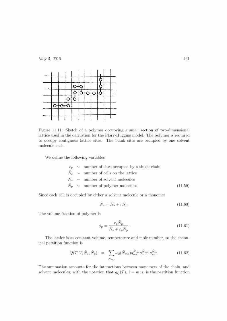
May 5, 2010 461
Figure 11.11: Sketch of a polymer occupying a small section of two-dimensionallattice used in the derivation for the Flory-Huggins model. The polymer is requiredto occupy contiguous lattice sites. The blank sites are occupied by one solventmolecule each.
We define the following variables
rp ∼ number of sites occupied by a single chain
Nc ∼ number of cells on the lattice
Ns ∼ number of solvent molecules
Np ∼ number of polymer molecules (11.59)
Since each cell is occupied by either a solvent molecule or a monomer
Nc = Ns + rNp. (11.60)
The volume fraction of polymer is
φp =rpNp
Ns + rpNp
. (11.61)
The lattice is at constant volume, temperature and mole number, so the canon-ical partition function is
Q(T, V, Ns, Np) =∑
Nms
ωd(Nms)qNmsms qNmmmm qNssss . (11.62)
The summation accounts for the interactions between monomers of the chain, andsolvent molecules, with the notation that qij(T ), i = m, s, is the partition function
462 Chapter 11: Thermodynamics of Polymers
for the interaction of two species, either monomer or solvent, and Nij is the numberof such pairs. As before, ωd(Nms; Nm, Ns) is the degeneracy, or number of confor-mations that lead to Nms monomer/solvent pair interactions when there are thegiven number of monomers and solvent molecules.
We now make the same approximation used to derive the Margules model fromChapter 9. Namely, we assume that the monomers and solvent molecules are ran-domly distributed on the lattice, so that we can write
Q(T, V, Ns, Np) ∼=∑
Nms
ωd(Nms)q〈Nms〉ms q〈Nmm〉
mm q〈Nss〉ss ,
= q〈Nms〉ms q〈Nmm〉mm q〈Nss〉ss
∑
Nms
ωd(Nms),
= q〈Nms〉ms q〈Nmm〉mm q〈Nss〉ss Ω, (11.63)
Ω is the number of possible microstates, and the angular brackets 〈. . .〉 indicate anaverage. We approximate this average using the random phase approximation. Nss
is the number of solvent/solvent pairs on the lattice, and we use similar notationfor the other types of pairs. We estimate these pairs assuming that the sites arerandomly occupied
〈Nms〉 ∼= (number of cells occupied by monomer)×(number of adjacent cells)×(fraction of those cells occupied by solvent)
= rNp(zl − 2)(1 − φp),
= (zl − 2)φp(1− φp)Nc. (11.64)
Recall that the coordination number of the lattice is assumed to be zl. Since thechain is contiguous, there are only (zl− 2) cells adjacent to a monomer that are notnecessarily occupied by another monomer. We neglect the small corrections fromthe chain ends. We can do something similar for the other pairs, being careful notto double count
〈Nss〉 ∼= Nszl(1− φp)1
2=
1
2zl(1− φp)
2Nc,
〈Nmm〉 ∼= rNp(zl − 2)φp1
2=
1
2(zl − 2)φ2pNc (11.65)
To estimate the number of possible microstates, we count how many ways arepossible to add the first chain, times the number of ways to add the second chain,
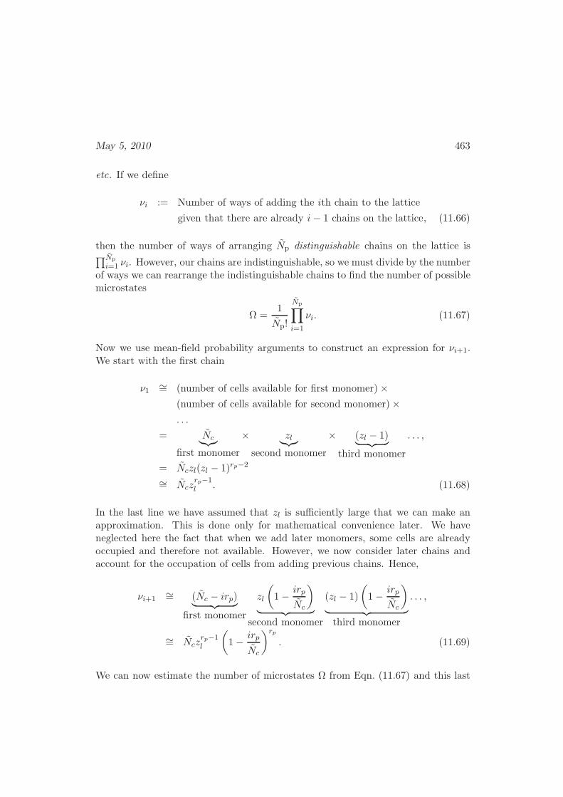
May 5, 2010 463
etc. If we define
νi := Number of ways of adding the ith chain to the lattice
given that there are already i− 1 chains on the lattice, (11.66)
then the number of ways of arranging Np distinguishable chains on the lattice is∏Np
i=1 νi. However, our chains are indistinguishable, so we must divide by the numberof ways we can rearrange the indistinguishable chains to find the number of possiblemicrostates
Ω =1
Np!
Np∏
i=1
νi. (11.67)
Now we use mean-field probability arguments to construct an expression for νi+1.We start with the first chain
ν1 ∼= (number of cells available for first monomer)×(number of cells available for second monomer)×. . .
= Nc︸︷︷︸
first monomer
× zl︸︷︷︸
second monomer
× (zl − 1)︸ ︷︷ ︸
third monomer
. . . ,
= Nczl(zl − 1)rp−2
∼= Nczrp−1l . (11.68)
In the last line we have assumed that zl is sufficiently large that we can make anapproximation. This is done only for mathematical convenience later. We haveneglected here the fact that when we add later monomers, some cells are alreadyoccupied and therefore not available. However, we now consider later chains andaccount for the occupation of cells from adding previous chains. Hence,
νi+1∼= (Nc − irp)
︸ ︷︷ ︸
first monomer
zl
(
1− irp
Nc
)
︸ ︷︷ ︸
second monomer
(zl − 1)
(
1− irp
Nc
)
︸ ︷︷ ︸
third monomer
. . . ,
∼= Nczrp−1l
(
1− irp
Nc
)rp
. (11.69)
We can now estimate the number of microstates Ω from Eqn. (11.67) and this last
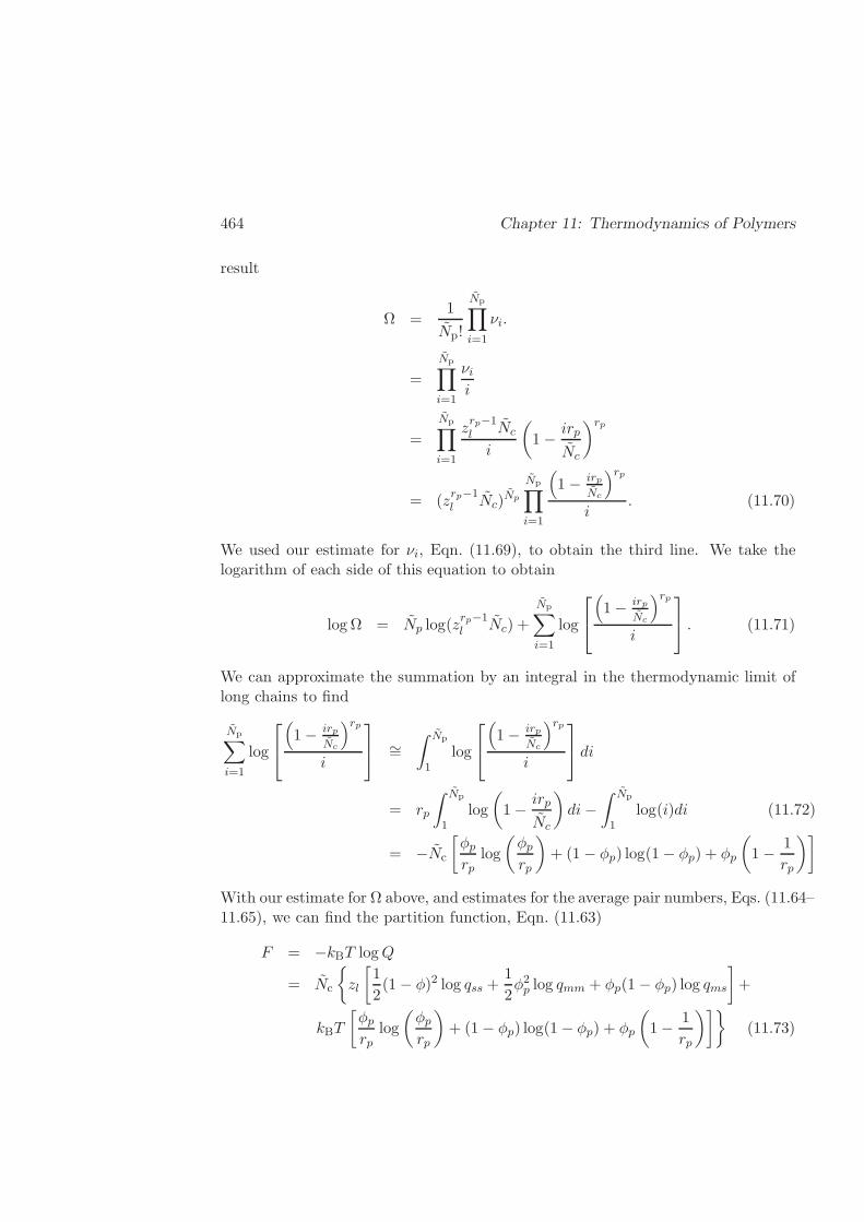
464 Chapter 11: Thermodynamics of Polymers
result
Ω =1
Np!
Np∏
i=1
νi.
=
Np∏
i=1
νii
=
Np∏
i=1
zrp−1l Nc
i
(
1− irp
Nc
)rp
= (zrp−1l Nc)
Np
Np∏
i=1
(
1− irpNc
)rp
i. (11.70)
We used our estimate for νi, Eqn. (11.69), to obtain the third line. We take thelogarithm of each side of this equation to obtain
log Ω = Np log(zrp−1l Nc) +
Np∑
i=1
log
(
1− irpNc
)rp
i
. (11.71)
We can approximate the summation by an integral in the thermodynamic limit oflong chains to find
Np∑
i=1
log
(
1− irpNc
)rp
i
∼=∫ Np
1log
(
1− irpNc
)rp
i
di
= rp
∫ Np
1log
(
1− irp
Nc
)
di−∫ Np
1log(i)di (11.72)
= −Nc
[φprp
log
(φprp
)
+ (1− φp) log(1− φp) + φp
(
1− 1
rp
)]
With our estimate for Ω above, and estimates for the average pair numbers, Eqs. (11.64–11.65), we can find the partition function, Eqn. (11.63)
F = −kBT logQ
= Nc
zl
[1
2(1− φ)2 log qss +
1
2φ2p log qmm + φp(1− φp) log qms
]
+
kBT
[φprp
log
(φprp
)
+ (1− φp) log(1− φp) + φp
(
1− 1
rp
)]
(11.73)
May 5, 2010 465
This is our estimate for the free energy of an amorphous mixture of polymer andsolvent. To estimate the free energy of mixing, we need the free energy for puresolvent and pure polymer. These may be found from the above expression in theappropriate limits: fpure solvent = F (φp → 0)/Nc and fpure polymer = rpF (φp →1)/Nc. Using the definition of mixing, ∆Fmix = F −Npf
pure polymer−Nsfpure solvent,
we obtain after some algebra
∆Fmix
NcRT= (1− φp) log(1− φp) +
φprp
log(φp) + χ(T )φp(1− φp), (11.74)
where
χ(T ) :=zl2log
(qms(T )
2
qmm(T )qss(T )
)
(11.75)
is called the Flory-Huggins interaction parameter. This derivation assumedthat solvent was present instead of two polymer species. If we make the samespecification to Eqn. (11.1) and assume incompressibility, these two expressions areequivalent.
11.5 Summary
In this chapter we introduced
• Mixing models for polymers, beginning with the Flory-Huggins fundamentalrelation for polymer liquids (§11.1). In §11.1 we used the Flory-Huggins modelto predict the spinodal and binodal curves for polymer solutions. There we sawhow volume fraction plays an important role in explaining the large asymmetryseen in these stability curves.
However, the Flory-Huggins model is not sufficiently accurate to describe ex-perimental data, so we also considered two generalizations in §11.2. Thefirst adds ad hoc parameters to describe the rich behavior seen experimen-tally for nearly incompressible polymer liquids. This generalization to theFlory-Huggins model was shown to describe the miscibility curve for a mix-ture of copolymer poly(vinyl alcohol)93-co-(vinyl acetate)7 , supercritical CO2
in polypropylene. The Sanchez-Lacombe model generalizes the Flory-Hugginsmodel to compressible polymer solutions, which was then used to predict thedensity of a mixture of polypropylene and supercritical CO2. A SAFT modelwas also introduced.
• Microphase separation in block copolymers. In §11.3, we showed how simplethermodynamic arguments can be used to make qualitative predictions aboutthe formation of microphases in block copolymers.
466 Chapter 11: Thermodynamics of Polymers
• A statistical mechanical derivation for the Flory-Huggins model in §11.4.
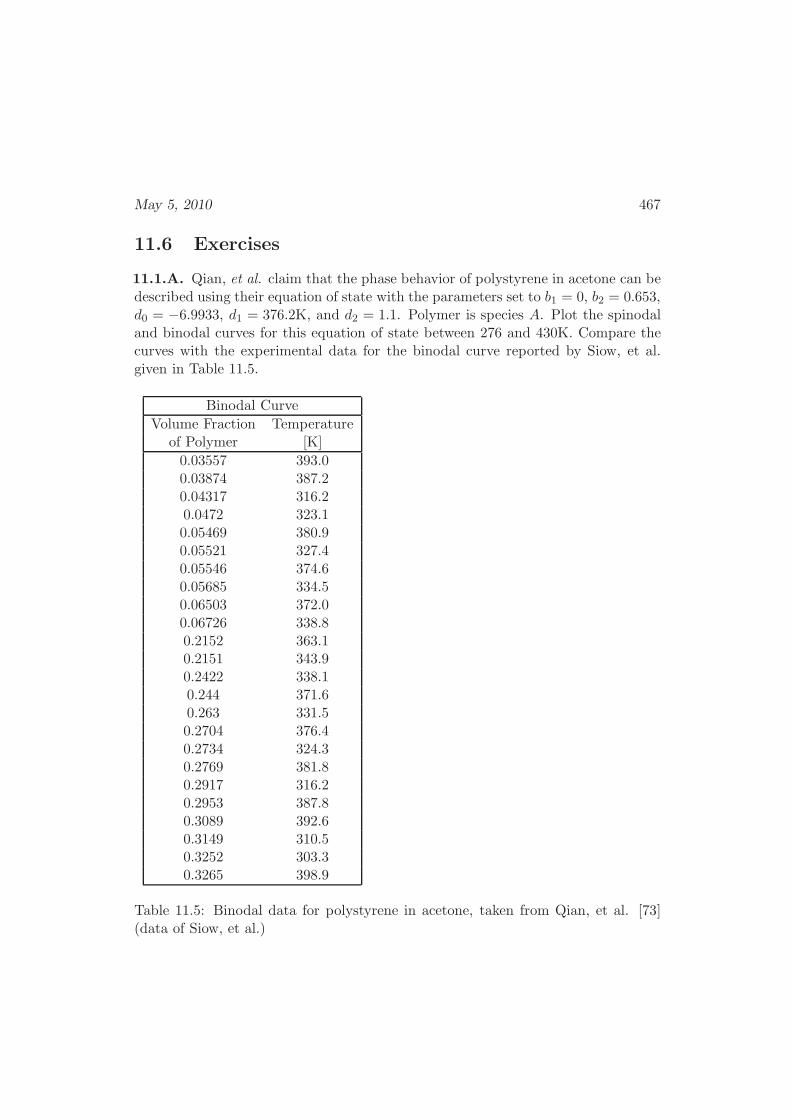
May 5, 2010 467
11.6 Exercises
11.1.A. Qian, et al. claim that the phase behavior of polystyrene in acetone can bedescribed using their equation of state with the parameters set to b1 = 0, b2 = 0.653,d0 = −6.9933, d1 = 376.2K, and d2 = 1.1. Polymer is species A. Plot the spinodaland binodal curves for this equation of state between 276 and 430K. Compare thecurves with the experimental data for the binodal curve reported by Siow, et al.given in Table 11.5.
Binodal Curve
Volume Fraction Temperatureof Polymer [K]
0.03557 393.00.03874 387.20.04317 316.20.0472 323.10.05469 380.90.05521 327.40.05546 374.60.05685 334.50.06503 372.00.06726 338.80.2152 363.10.2151 343.90.2422 338.10.244 371.60.263 331.50.2704 376.40.2734 324.30.2769 381.80.2917 316.20.2953 387.80.3089 392.60.3149 310.50.3252 303.30.3265 398.9
Table 11.5: Binodal data for polystyrene in acetone, taken from Qian, et al. [73](data of Siow, et al.)
468 Chapter 11: Thermodynamics of Polymers
11.1.B. Derive an equation for the binodal points from the Flory-Huggins equation.
11.1.C. Using the Sanchez-Lacombe equation, find the solubility of CO2 at a pres-sure of 500 MPa.
Hint: You should be able to reduce the problem to two coupled, nonlinear algebraicequations. The roots to these equations can be found iteratively by guessing a valuefor the solubility, and iterating.
11.1.D. Prove that the expression for the chemical potential, Eqn. (11.43) is correct.
11.1.E. Sanchez and Panayiotou [66] have proposed a somewhat simpler model forcompressible polymer solutions
G = rN
P vv∗ − ǫ∗
v+RT
[
(v − 1) log
(v − 1
v
)
− 1
rlog v+
φ1r1
log φ1 +φ2r2
log φ2
]
. (11.76)
The mixing rules for this model are
ǫ∗ = φ1ǫ∗1 + φ1ǫ
∗2 − φ1φ2RTχ12,
v∗ = φ1v∗1 + φ2v
∗2. (11.77)
The new parameters are related to the others by the relations
ǫ∗i = RT ∗i ,
v∗i =RT ∗
i
P ∗i
. (11.78)
Find an expression for the chemical potential of species 1 as a function of T , P andφ2. Note that an implicit expression for v is needed for this model, as well.
11.1.F. Verify the expression for the PV T equation of state from the BGK model,Eqn. (11.47).
11.1.G. Find the parameters of the BGK model for poly(methyl vinyl ether). Com-pressibility data can be found in their paper.
11.3.A We need examples for cylindrical structures with block copoly-mers.
Chapter 12
Thermodynamics of Surfaces
The pressure inside a soap bubble is slightly larger than that outside the bubble. Ifthe pressure inside the bubble were the same as outside the bubble, it would simplycollapse. The liquid film that constitutes the bubble is under tension, and is there-fore able to sustain the force imbalance that arises from that pressure difference.Throughout most of this text, we have focused our attention on the properties ofbulk phases. The boundaries or interfacial regions between bulk phases at equilib-rium exhibit a number of interesting properties that are, in general, different fromthose of the bulk. These properties are particularly important in a wide varietyof technologies, including nano-fabrication, ink-jet printing, or biotechnology. Thefollowing chapter discusses a few extensions of ideas presented earlier in the text todetermine the behavior of interfaces.
The study of the thermodynamics of surfaces usually adopts one of two conven-tions. In the approach of Gibbs, a sharp dividing surface is introduced between twodistinct phases (e.g. a vapor and a liquid). In the approach of Guggenheim, the in-terfacial region has a finite volume V σ, over which the thermodynamic properties ofthe system change gradually. The latter approach is followed closely in this chapterbecause it is more physically intuitive. We note, however, that in our discussion ofmixtures and surface quantities we adopt the view that the volume of the interfacialregion is so small as to be negligible. In that limit, we implicitly return to the Gibbstreatment of an interface.
12.1 Interfacial Tension of a Planar Interface
Consider two distinct bulk phases, α and β, separated by a planar interfacial regiondenoted by σ (See Figure 12.1). That interfacial region is bounded by two planes,AA′ and BB′. In any bulk phase, the pressure is uniform; that is, the force per
469
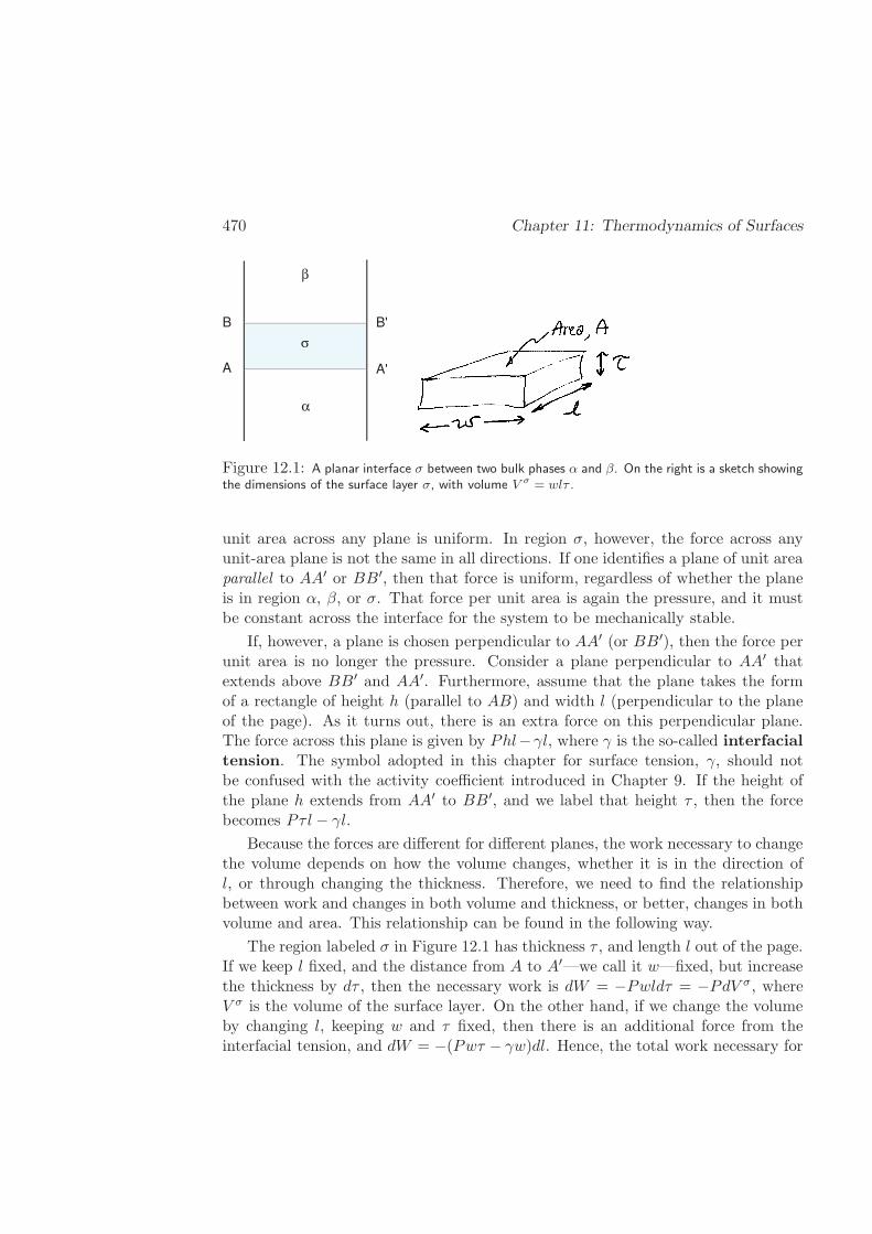
470 Chapter 11: Thermodynamics of Surfaces
σ
B B'
A A'
α
β
Figure 12.1: A planar interface σ between two bulk phases α and β. On the right is a sketch showingthe dimensions of the surface layer σ, with volume V σ = wlτ .
unit area across any plane is uniform. In region σ, however, the force across anyunit-area plane is not the same in all directions. If one identifies a plane of unit areaparallel to AA′ or BB′, then that force is uniform, regardless of whether the planeis in region α, β, or σ. That force per unit area is again the pressure, and it mustbe constant across the interface for the system to be mechanically stable.
If, however, a plane is chosen perpendicular to AA′ (or BB′), then the force perunit area is no longer the pressure. Consider a plane perpendicular to AA′ thatextends above BB′ and AA′. Furthermore, assume that the plane takes the formof a rectangle of height h (parallel to AB) and width l (perpendicular to the planeof the page). As it turns out, there is an extra force on this perpendicular plane.The force across this plane is given by Phl−γl, where γ is the so-called interfacialtension. The symbol adopted in this chapter for surface tension, γ, should notbe confused with the activity coefficient introduced in Chapter 9. If the height ofthe plane h extends from AA′ to BB′, and we label that height τ , then the forcebecomes Pτl − γl.
Because the forces are different for different planes, the work necessary to changethe volume depends on how the volume changes, whether it is in the direction ofl, or through changing the thickness. Therefore, we need to find the relationshipbetween work and changes in both volume and thickness, or better, changes in bothvolume and area. This relationship can be found in the following way.
The region labeled σ in Figure 12.1 has thickness τ , and length l out of the page.If we keep l fixed, and the distance from A to A′—we call it w—fixed, but increasethe thickness by dτ , then the necessary work is dW = −Pwldτ = −PdV σ, whereV σ is the volume of the surface layer. On the other hand, if we change the volumeby changing l, keeping w and τ fixed, then there is an additional force from theinterfacial tension, and dW = −(Pwτ − γw)dl. Hence, the total work necessary for
May 5, 2010 471
changing τ and l independently (with fixed w) is
dW = −Pwldτ − (Pwτ − γw)dl, fixed w,
= −P (wldτ + wτdl) + γwdl, fixed w,
= −Pd(wlτ) + γd(wl), fixed w,
= −PdV σ + γdA. (12.1)
The last line is our desired result. We now know the work necessary to change eitherthe volume or the area of the surface layer at fixed temperature and mole numbers.
The differential of the Helmholtz free energy of a bulk phase is given by anexpression of the form
dF = −SdT − PdV +∑
i
µidNi. (12.2)
For a surface phase, the work term, PdV , appearing in Eqn. (12.2) is replaced bythat given in Eqn. (12.1) to give the following equation for the differential of theHelmholtz free energy of a surface phase
dF σ = −SσdT − PdV σ + γdA+∑
i
µidNσi . (12.3)
In fact, we now have a thermodynamic definition for the interfacial tension,
γ ≡(∂F σ
∂A
)
T,V σ ,Ni, (12.4)
as the change in free energy with surface area at fixed temperature, volume andmole numbers.
It is instructive to consider the molecular origins of the interfacial tension. Ina bulk liquid, an individual molecule is completely surrounded by other molecules.As discussed in earlier chapters, all molecules in the liquid exert an attractive forceon each other. At a liquid-vapor interface, however, this physical picture is altered.Molecules at the interface are only partially surrounded by other molecules, becauseof the lower density of the “vapor” side. It is therefore energetically unfavorablefor a molecule to sit at the interface, and work must be done to drag a moleculefrom the bulk of the liquid phase to that interface; the interfacial energy can beinterpreted as the energy (per unit of surface area) required for such process.
472 Chapter 11: Thermodynamics of Surfaces
12.2 Gibbs Free Energy of a Surface Phase and Gibbs-
Duhem Relation
In order to arrive at an expression for the Gibbs free energy of a surface phase, wenote that the Helmholtz potential is extensive in the surface area
F σ(T, λV σ, λA, λNσi ) = λF σ(T, V σ, A,Nσ
i ) (12.5)
Therefore, similar to what we have already seen for bulk systems, we can write (seethe derivation of the Euler relation, Eqn. (3.20))
F σ = −PV σ + γA+∑
i
µiNσi . (12.6)
Equation (12.6) should be contrasted to the analogous expression for a bulk phase,namely F + PV = G =
∑
i µiNσi . For a surface phase, the Gibbs free energy
differs from that of a bulk phase by an additional term consisting of the product ofinterfacial tension and area:
Gσ = F σ + PV σ − γA
=∑
i
µiNσi . (12.7)
Alternatively, the above expression can be viewed as a Legendre transform of F inboth volume and area (§3.1). The differential of the Gibbs free energy is given by
dGσ = −SσdT + PdV σ −Adγ +∑
i
µidNσi (12.8)
Equation (12.6) can be differentiated to give
dF σ + PdV σ + V σdP − γdA−Adγ =∑
i
µidNσi +
∑
i
Nσi dµi. (12.9)
Equation (12.9) can be subtracted from (12.3) to give
0 = SσdT − V σdP +Adγ +∑
i
Nσi dµi. (12.10)
Equation (12.10) is the surface analog of the Gibbs-Duhem equation, Eqn. (3.22)presented in §3.1.
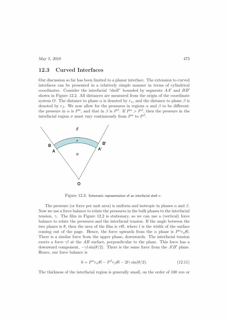
May 5, 2010 473
12.3 Curved Interfaces
Our discussion so far has been limited to a planar interface. The extension to curvedinterfaces can be presented in a relatively simple manner in terms of cylindricalcoordinates. Consider the interfacial “shell” bounded by segments AA′ and BB′
shown in Figure 12.2. All distances are measured from the origin of the coordinatesystem O. The distance to phase α is denoted by rα, and the distance to phase β isdenoted by rβ . We now allow for the pressures in regions α and β to be different:the pressure in α is Pα, and that in β is P β. If Pα > P β, then the pressure in theinterfacial region σ must vary continuously from Pα to P β.
Figure 12.2: Schematic representation of an interfacial shell σ.
The pressure (or force per unit area) is uniform and isotropic in phases α and β.Now we use a force balance to relate the pressures in the bulk phases to the interfacialtension, γ. The film in Figure 12.2 is stationary, so we can use a (vertical) forcebalance to relate the pressures and the interfacial tension. If the angle between thetwo planes is θ, then the area of the film is rθl, where l is the width of the surfacecoming out of the page. Hence, the force upwards from the α phase is Pαrαθl.There is a similar force from the upper phase, downwards. The interfacial tensionexerts a force γl at the AB surface, perpendicular to the plane. This force has adownward component, −γl sin(θ/2). There is the same force from the A′B′ plane.Hence, our force balance is
0 = Pαrαθl− P βrβθl− 2lγ sin(θ/2). (12.11)
The thickness of the interfacial region is generally small, on the order of 100 nm or
474 Chapter 11: Thermodynamics of Surfaces
less. The difference between rα and rβ therefore typically satisfies the inequality,
rβ − rα ≪ r, (12.12)
where
r =rα + rβ
2. (12.13)
Therefore, we replace both rα and rβ with r in Eqn. (12.11) and take the limit θ → 0to obtain
Pα − P β =γ
r. (12.14)
A similar exercise can be performed for a spherical interface, in which case Equation(12.14) becomes
Pα − P β = 2γ
r. (12.15)
The derivation outlined here can be extended to curved interfaces of arbitrary shape,with the general result
Pα − P β = γ
(1
r1+
1
r2
)
, (12.16)
where r1 and r2 denote the principal radii of curvature of the interface. Equation(12.16) is known as the Young-Laplace equation, first derived approximately 200years ago.
Equation (12.15) can now be used to determine the pressure difference betweenthe exterior of a bubble, Pext, and the interior of a bubble, Pint. Note that a bubblehas two interfaces: air-film-air. If the pressure in the film itself is denoted by P ′, wehave
Pint − P ′ = 2γ
rint
P ′ − Pext = 2γ
rext(12.17)
and therefore
Pint − Pext = γ
(2
rint+
2
rext
)
. (12.18)
By neglecting the difference between rint and rext, one arrives at the following ex-pression for the sought-after pressure difference:
Pint − Pext = 4γ
r. (12.19)
Table 12.1 gives values of the surface tension for several common liquids. Waterhas relatively large surface tension. Simple alkanes have a surface tension that is
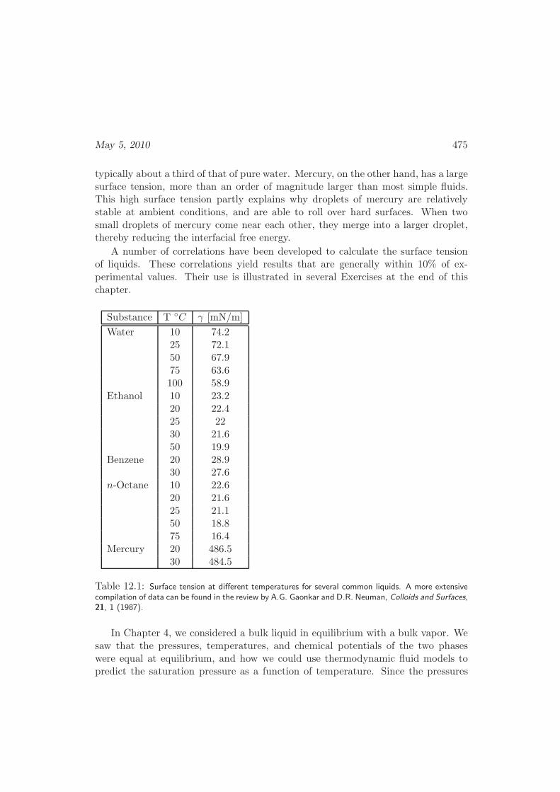
May 5, 2010 475
typically about a third of that of pure water. Mercury, on the other hand, has a largesurface tension, more than an order of magnitude larger than most simple fluids.This high surface tension partly explains why droplets of mercury are relativelystable at ambient conditions, and are able to roll over hard surfaces. When twosmall droplets of mercury come near each other, they merge into a larger droplet,thereby reducing the interfacial free energy.
A number of correlations have been developed to calculate the surface tensionof liquids. These correlations yield results that are generally within 10% of ex-perimental values. Their use is illustrated in several Exercises at the end of thischapter.
Substance T C γ [mN/m]
Water 10 74.225 72.150 67.975 63.6100 58.9
Ethanol 10 23.220 22.425 2230 21.650 19.9
Benzene 20 28.930 27.6
n-Octane 10 22.620 21.625 21.150 18.875 16.4
Mercury 20 486.530 484.5
Table 12.1: Surface tension at different temperatures for several common liquids. A more extensivecompilation of data can be found in the review by A.G. Gaonkar and D.R. Neuman, Colloids and Surfaces,21, 1 (1987).
In Chapter 4, we considered a bulk liquid in equilibrium with a bulk vapor. Wesaw that the pressures, temperatures, and chemical potentials of the two phaseswere equal at equilibrium, and how we could use thermodynamic fluid models topredict the saturation pressure as a function of temperature. Since the pressures
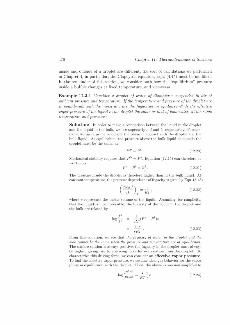
476 Chapter 11: Thermodynamics of Surfaces
inside and outside of a droplet are different, the sort of calculations we performedin Chapter 4, in particular, the Clapeyron equation, Eqn. (4.45) must be modified.In the remainder of this section, we consider both how the “equilibrium” pressureinside a bubble changes at fixed temperature, and vice-versa.
Example 12.3.1 Consider a droplet of water of diameter r suspended in air atambient pressure and temperature. If the temperature and pressure of the droplet arein equilibrium with the moist air, are the fugacities in equilibrium? Is the effectivevapor pressure of the liquid in the droplet the same as that of bulk water, at the sametemperature and pressure?
Solution: In order to make a comparison between the liquid in the dropletand the liquid in the bulk, we use superscripts d and b, respectively. Further-more, we use a prime to denote the phase in contact with the droplet and thebulk liquid. At equilibrium, the pressure above the bulk liquid or outside thedroplet must be the same, i.e.
P d′ = P b′ . (12.20)
Mechanical stability requires that P b′ = P b. Equation (12.15) can therefore bewritten as
P d − P b = 2γ
r. (12.21)
The pressure inside the droplet is therefore higher than in the bulk liquid. Atconstant temperature, the pressure dependence of fugacity is given by Eqn. (8.43)
(d log f
dP
)
T
=v
RT, (12.22)
where v represents the molar volume of the liquid. Assuming, for simplicity,that the liquid is incompressible, the fugacity of the liquid in the droplet andthe bulk are related by
logfd
f b=
1
RT(P d − P b)v
=2γv
rRT. (12.23)
From this equation, we see that the fugacity of water in the droplet and thebulk cannot be the same when the pressure and temperature are at equilibrium.The surface tension is always positive; the fugacity in the droplet must alwaysbe higher, giving rise to a driving force for evaporation from the droplet. Tocharacterize this driving force, we can consider an effective vapor pressure.To find the effective vapor pressure, we assume ideal gas behavior for the vaporphase in equilibrium with the droplet. Then, the above expression simplifies to
logP d,sat
P b,sat=
2
RT
γ
rv . (12.24)
May 5, 2010 477
Equation (12.24) represents an approximate form (ideal gas behavior was as-sumed) of the so-calledKelvin equation. These results show that, at the sameexternal pressure and temperature, the vapor pressure (and fugacity) of a liquidin a droplet is higher than that in the bulk. This difference in vapor pressureswill cause the liquid in the droplet to evaporate faster, thereby decreasing itsradius and increasing the vapor pressure difference even more. The equilibriumbetween small droplets and the bulk is therefore unstable, and eventually smalldroplets disappear. In the case of multiple droplets of different diameters, thelarger droplets will grow at the expense of the smaller ones.
In the particular case of water at 25C and 1 bar, the surface tension isγ = 72 dynes/cm. In a 1 µ m droplet, the vapor pressure of water increases bya factor of 1.001; in a 10 nm droplet, it increases by a factor of 1.1 . 2
In the last example, we found that it is not possible for the temperature, pressureand fugacity in the droplet to be in equilibrium with a vapor phase that is inequilibrium with a bulk liquid phase. If we assumed that the temperature andpressure are in equilibrium, we could find the effective equilibrium vapor pressurein the droplet at fixed temperature.
Now we consider how the equilibrium temperature changes with fixed vaporpressure, if the fugacities and pressures are in equilibrium. The chemical potentialsand temperatures of the two phases are equal at equilibrium. The calculation weperform is to keep the pressure of the vapor constant, and see how the equilibrium‘saturation temperature’ changes with radius, at a fixed vapor pressure.
Towards this end, similar to the Clapeyron equation, we begin with the Gibbs-Duhem relation for the liquid and vapor phases, Eqn. (4.44)
(sv − sl)dT + vldP l = 0 , constant P v, (12.25)
where we have set dP v = 0 because the external pressure is constant. Furthermore,from the Young-Laplace equation we write
dP l = d
(2γ
r
)
, constant P v. (12.26)
Given that sv − sl = ∆hvap/T , Eqn. (12.25) can be integrated from some finite rvalue to r = ∞ to arrive at the following expression for the equilibrium temperaturedependence on droplet size
logT
T0∼= − 2vlγ
∆hvapr. (12.27)
Here T0 is the temperature at r = ∞, and we assumed constant vl and hvap. Equa-tion (12.27) is known as the Thomson equation. To derive it, we assumed that∆hvap and vl are independent of temperature.
478 Chapter 11: Thermodynamics of Surfaces
The Thomson equation indicates that, as the size of the droplet decreases, thetemperature required to establish chemical equilibrium across the interface decreases(T < T0 because ∆h
vap is always positive). For the vapor to condense into the liquiddroplet, it must be cooled down to a temperature below the normal condensationtemperature corresponding to temperature P v. In other words, the vapor must besupercooled.
12.4 Capillary Forces
Capillary forces are ubiquitous not only in science and engineering, but also ineveryday life. Capillary forces are intimately related to surface thermodynamics,and in fact they provide a simple means to measure surface tension.
Figure 12.3 shows a schematic representation of a capillary tube above a liquidphase α. The surface BB′, or meniscus, can be regarded as a segment of a spherewith origin O. The angle between the radius of the sphere OB and the horizontalline OX, the so-called contact angle, is denoted by θ. The radius of curvature ofBB′ is given by r/ cos θ.
Figure 12.3: Schematic representation of a capillary tube above a liquid phase.
The pressures of both phases α and β are the same at A, and denoted by P 0.The pressure at position A in the capillary is also P 0. The pressure at the BB′
interface in the capillary is denoted by Pα in phase α and P β in phase β. If Ldenotes the height of the liquid in the capillary (i.e., the distance AB), and ρα andρβ denote the densities of phases α and β, then the pressures are just hydrostatic
Pα = P 0 − ρα|~g|LP β = P 0 − ρβ|~g|L, (12.28)
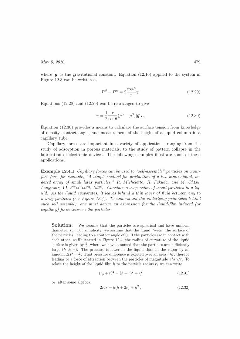
May 5, 2010 479
where |~g| is the gravitational constant. Equation (12.16) applied to the system inFigure 12.3 can be written as
P β − Pα = 2cos θ
rγ. (12.29)
Equations (12.28) and (12.29) can be rearranged to give
γ =1
2
r
cos θ(ρα − ρβ)|~g|L. (12.30)
Equation (12.30) provides a means to calculate the surface tension from knowledgeof density, contact angle, and measurement of the height of a liquid column in acapillary tube.
Capillary forces are important in a variety of applications, ranging from thestudy of adsorption in porous materials, to the study of pattern collapse in thefabrication of electronic devices. The following examples illustrate some of theseapplications.
Example 12.4.1 Capillary forces can be used to “self-assemble” particles on a sur-face (see, for example, “A simple method for production of a two-dimensional, or-dered array of small latex particles,” R. Micheletto, H. Fukuda, and M. Ohtsu,Langmuir, 11, 3333-3336, 1995). Consider a suspension of small particles in a liq-uid. As the liquid evaporates, it leaves behind a thin layer of fluid between any tonearby particles (see Figure 12.4). To understand the underlying principles behindsuch self assembly, one must derive an expression for the liquid-film induced (orcapillary) force between the particles.
Solution: We assume that the particles are spherical and have uniformdiameter, rp. For simplicity, we assume that the liquid “wets” the surface ofthe particles, leading to a contact angle of 0. If the particles are in contact witheach other, as illustrated in Figure 12.4, the radius of curvature of the liquidsurface is given by 1
r , where we have assumed that the particles are sufficientlylarge (h ≫ r). The pressure is lower in the liquid than in the vapor by anamount ∆P = γ
r . That pressure difference is exerted over an area πhr, therebyleading to a force of attraction between the particles of magnitude πhrγ/r. Torelate the height of the liquid film h to the particle radius rp we can write
(rp + r)2 = (h+ r)2 + r2p (12.31)
or, after some algebra,
2rpr = h(h+ 2r) ≈ h2 , (12.32)
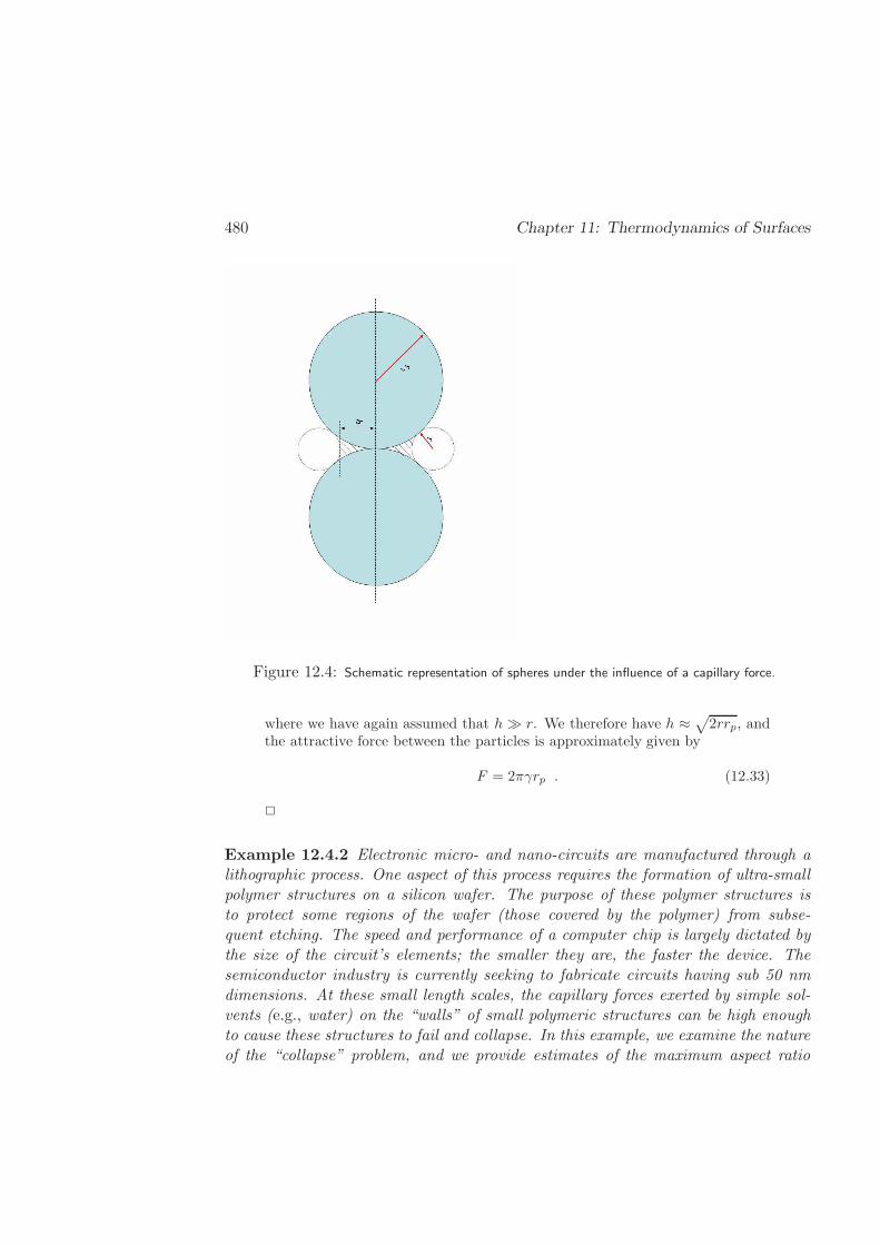
480 Chapter 11: Thermodynamics of Surfaces
Figure 12.4: Schematic representation of spheres under the influence of a capillary force.
where we have again assumed that h ≫ r. We therefore have h ≈√2rrp, and
the attractive force between the particles is approximately given by
F = 2πγrp . (12.33)
2
Example 12.4.2 Electronic micro- and nano-circuits are manufactured through alithographic process. One aspect of this process requires the formation of ultra-smallpolymer structures on a silicon wafer. The purpose of these polymer structures isto protect some regions of the wafer (those covered by the polymer) from subse-quent etching. The speed and performance of a computer chip is largely dictated bythe size of the circuit’s elements; the smaller they are, the faster the device. Thesemiconductor industry is currently seeking to fabricate circuits having sub 50 nmdimensions. At these small length scales, the capillary forces exerted by simple sol-vents (e.g., water) on the “walls” of small polymeric structures can be high enoughto cause these structures to fail and collapse. In this example, we examine the natureof the “collapse” problem, and we provide estimates of the maximum aspect ratio
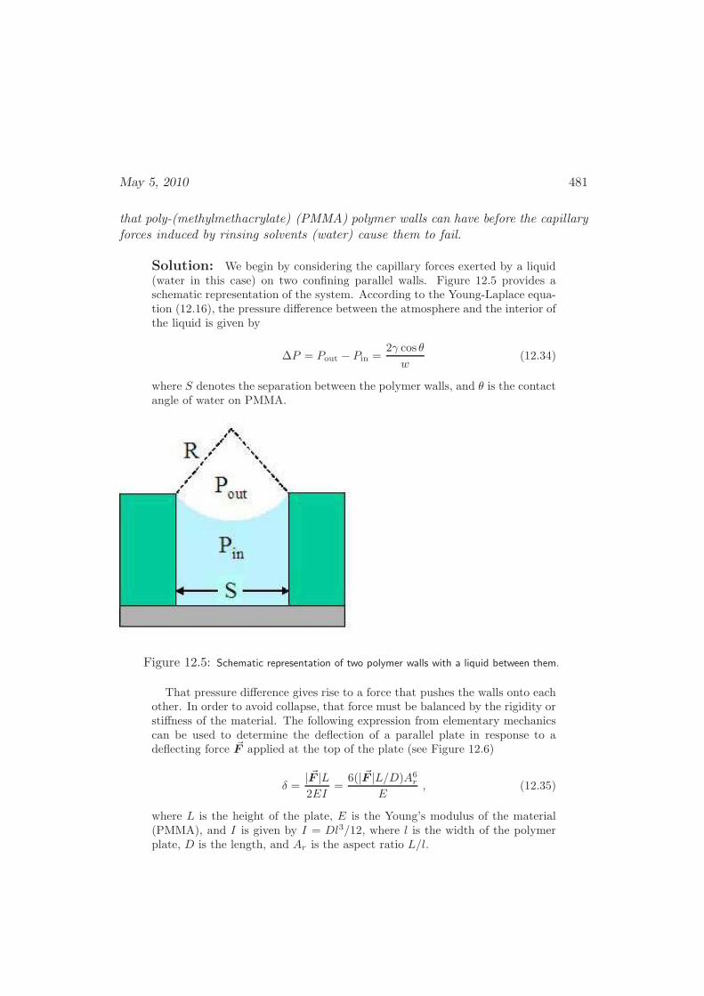
May 5, 2010 481
that poly-(methylmethacrylate) (PMMA) polymer walls can have before the capillaryforces induced by rinsing solvents (water) cause them to fail.
Solution: We begin by considering the capillary forces exerted by a liquid(water in this case) on two confining parallel walls. Figure 12.5 provides aschematic representation of the system. According to the Young-Laplace equa-tion (12.16), the pressure difference between the atmosphere and the interior ofthe liquid is given by
∆P = Pout − Pin =2γ cos θ
w(12.34)
where S denotes the separation between the polymer walls, and θ is the contactangle of water on PMMA.
Figure 12.5: Schematic representation of two polymer walls with a liquid between them.
That pressure difference gives rise to a force that pushes the walls onto eachother. In order to avoid collapse, that force must be balanced by the rigidity orstiffness of the material. The following expression from elementary mechanicscan be used to determine the deflection of a parallel plate in response to adeflecting force ~F applied at the top of the plate (see Figure 12.6)
δ =| ~F |L2EI
=6(| ~F |L/D)A6
r
E, (12.35)
where L is the height of the plate, E is the Young’s modulus of the material(PMMA), and I is given by I = Dl3/12, where l is the width of the polymerplate, D is the length, and Ar is the aspect ratio L/l.
482 Chapter 11: Thermodynamics of Surfaces
Figure 12.6: Schematic representation of a polymer wall subject to a deflecting force applied at thetop.
For PMMA at 298 K, E = 3GPa, and the contact angle for water on PMMAis θ = 5[104]. Measuring the mechanical properties of small nano-scale poly-meric structures is notoriously challenging. These experiments must be con-ducted in a statistical manner, as minute differences between seemingly identicalstructures and small defects can give rise to large uncertainties. Figure 12.7shows the percentage of polymer structures that have collapsed as a functionof aspect ratio for PMMA lines of width l = 200 nm separated by a distanced = 200 nm. That figure allows us to identify a critical aspect ratio for collapse(CARC), beyond which the stiffness of the material is no longer sufficient tosustain the deflecting (capillary) forces brought about by the liquid. The resultsin that figure and the electron micro-graphs in Figure 12.8 show that beyonda “critical” aspect ratio of 4 the polymer walls start to collapse. The suddenincrease in the percent collapse at about AR = 4 is explained by the 3d powerdependence of the deflection on aspect ratio Eqn. (12.35).
Equations (12.29) and (12.35) provide the basis for the derivation of a para-metric equation that permits calculation of the CARC. The derivation of thatequation includes elements from mechanics that are beyond the scope of thistext, and can be found in the literature.
The results in Figure 12.7 provide the basis for creation of an ingenious,

May 5, 2010 483
Figure 12.7: Experimental data for the critical aspect ratio for collapse (CARC) for PMMA polymerwalls of line width l = 200 nm separated by a distance d = 200 nm.
Figure 12.8: Experimental electron micro-graphs of PMMA polymer walls of width l = 200 nmseparated by a distance d = 200 nm right below and right after the CARC.
capillary-force based test bed for measurement of the mechanical properties ofpolymeric systems in nano-scale geometries. Consider the geometries shownin Figure 12.9. Two polymer walls separated by an inner spacing IS are sur-rounded by two liquid pools of width OS (for Outer Spacing). The force exertedon the polymer walls by the liquid to their sides is given by
F = ∆P ×Area = 2γ cos θ
(1
IS− 1
OS
)
LD (12.36)
where, as before, L and D denote the height and the length of the polymerwalls. By controlling the dimensions of the capillary force device, it is possibleto tune the force that is applied to a material. When that force overcomes thestiffness of the polymer, the material collapses, as shown in Figure 12.10. Insuch a device, the critical aspect ratio for collapse is given by substituting theforce in Eqn. (12.36) into Eqn. (12.35).
2
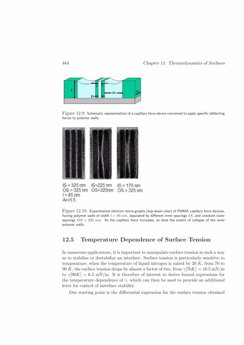
484 Chapter 11: Thermodynamics of Surfaces
Figure 12.9: Schematic representation of a capillary force device conceived to apply specific deflectingforces to polymer walls.
Figure 12.10: Experimental electron micro-graphs (top-down view) of PMMA capillary force devices,having polymer walls of width l = 85 nm, separated by different inner spacings IS, and constant outerspacings OS = 325 nm. As the capillary force increases, so does the extent of collapse of the innerpolymer walls.
12.5 Temperature Dependence of Surface Tension
In numerous applications, it is important to manipulate surface tension in such a wayas to stabilize or destabilize an interface. Surface tension is particularly sensitive totemperature; when the temperature of liquid nitrogen is raised by 20 K, from 70 to90 K, the surface tension drops by almost a factor of two, from γ[70K] = 10.5 mN/mto γ[90K] = 6.2 mN/m. It is therefore of interest to derive formal expressions forthe temperature dependence of γ, which can then be used to provide an additionallever for control of interface stability.
Our starting point is the differential expression for the surface tension obtained
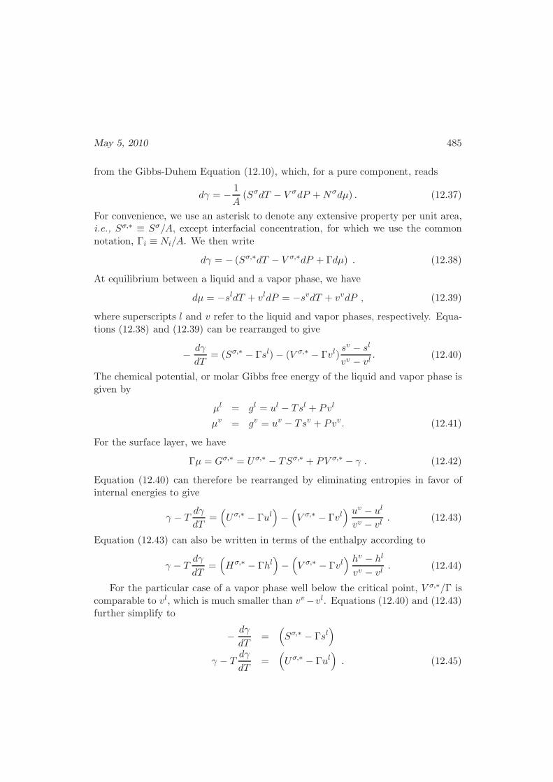
May 5, 2010 485
from the Gibbs-Duhem Equation (12.10), which, for a pure component, reads
dγ = − 1
A(SσdT − V σdP +Nσdµ) . (12.37)
For convenience, we use an asterisk to denote any extensive property per unit area,i.e., Sσ,∗ ≡ Sσ/A, except interfacial concentration, for which we use the commonnotation, Γi ≡ Ni/A. We then write
dγ = − (Sσ,∗dT − V σ,∗dP + Γdµ) . (12.38)
At equilibrium between a liquid and a vapor phase, we have
dµ = −sldT + vldP = −svdT + vvdP , (12.39)
where superscripts l and v refer to the liquid and vapor phases, respectively. Equa-tions (12.38) and (12.39) can be rearranged to give
− dγ
dT= (Sσ,∗ − Γsl)− (V σ,∗ − Γvl)
sv − sl
vv − vl. (12.40)
The chemical potential, or molar Gibbs free energy of the liquid and vapor phase isgiven by
µl = gl = ul − Tsl + Pvl
µv = gv = uv − Tsv + Pvv . (12.41)
For the surface layer, we have
Γµ = Gσ,∗ = Uσ,∗ − TSσ,∗ + PV σ,∗ − γ . (12.42)
Equation (12.40) can therefore be rearranged by eliminating entropies in favor ofinternal energies to give
γ − Tdγ
dT=(
Uσ,∗ − Γul)
−(
V σ,∗ − Γvl) uv − ul
vv − vl. (12.43)
Equation (12.43) can also be written in terms of the enthalpy according to
γ − Tdγ
dT=(
Hσ,∗ − Γhl)
−(
V σ,∗ − Γvl) hv − hl
vv − vl. (12.44)
For the particular case of a vapor phase well below the critical point, V σ,∗/Γ iscomparable to vl, which is much smaller than vv−vl. Equations (12.40) and (12.43)further simplify to
− dγ
dT=
(
Sσ,∗ − Γsl)
γ − Tdγ
dT=
(
Uσ,∗ − Γul)
. (12.45)
486 Chapter 11: Thermodynamics of Surfaces
The quantity(Sσ,∗ − Γsl
)represents the difference between the entropy per unit
area in the surface layer, and the entropy that the same surface layer would haveif it exhibited the properties of the bulk liquid. The surface tension decreases withtemperature. Experimental data for ∂γ
∂T for a wide array of liquids can be found inG. Korosi and E. Kovatz, J.Chem. Eng. Data, 26, 323 (1981). For water at ambientconditions, the temperature dependence is approximately ∂γ
∂T ≈ −138 × 10−3 mNm K .
For ethanol at ambient conditions, ∂γ∂T ≈ −86× 10−3 mN
m K .Several empirical correlations have been proposed to estimate the effect of tem-
perature on surface tension. The Eotvos correlation, proposed more than one hun-dred years ago (R. Eotvos, Weid Ann. 27, 456 (1886)), for example, relates γ tothe critical temperature and the molar volume according to
γ = k(Tc − T )
v1/3, (12.46)
where k is a constant with a value of 2.1 × 10⁻⁴mJ/K for many liquids. Severalmore recent correlations are given in the Exercises at the end of the chapter.
12.6 Interfaces in Mixtures
As one might expect, the composition of the interfacial region in a mixture is gener-ally different from that of the bulk. Different components exhibit different tendenciesto segregate to the interface, and as a result, the surface tension can exhibit a markeddependence on composition. Design of liquid or vapor phase separation processesoften requires that surface tension be determined as a function of composition; wenow derive formal expressions to do so. For concreteness, we derive expressions forthe temperature and composition dependence in binary mixtures; generalization tomulticomponent systems is discussed in the problems.
12.6.1 Vapor-Liquid Interfaces
We first consider the case of an interface between a liquid and a vapor phase. For atwo-component system, the differential of the surface tension is given by the Gibbs-Duhem equation (12.10)
− dγ = Sσ,∗dT − V σ,∗dP + Γ1dµ1 + Γ2dµ2 . (12.47)
Equation (12.47) can be simplified by assuming that the interfacial region is ex-tremely thin, so that the term PV σ,∗ becomes negligible. If we assume that thevolume of the interface V σ,∗ is small, at constant temperature that equation be-comes
dγ = −Γ1dµ1 − Γ2dµ2 . (12.48)
May 5, 2010 487
This equation is often referred to as the Gibbs adsorption isotherm.Also neglecting volume, the differential of the chemical potential for components
1 and 2 in the liquid phase can be written as
dµ1 = −S1dT + V1dP +
(∂µ1∂x2
)
T,P
dx2
dµ2 = −S2dT + V2dP +
(∂µ2∂x2
)
T,P
dx2 . (12.49)
Following our treatment for the temperature dependence of surface tension, weassume that PVi for a condensed phase is much smaller than RT . We also assumethat terms of the type PV σ,∗ are negligible. The two expressions above then simplifyto
dµ1 = −S1dT +
(∂µ1∂x2
)
T,P
dx2
dµ2 = −S2dT +
(∂µ2∂x2
)
T,P
dx2 . (12.50)
The surface tension can therefore be written in terms of the chemical potentials as
dγ = −(Sσ,∗ − Γ1S1 − Γ2S2
)dT −
[
Γ1
(∂µ1∂x2
)
T,P
+ Γ2
(∂µ2∂x2
)
T,P
]
dx2
= −(Sσ,∗ − Γ1S1 − Γ2S2
)dT −
(
Γ2 − Γ1x2
1− x2
)(∂µ2∂x2
)
T,P
dx2 .(12.51)
To derive Eqn. (12.51), we used the Gibbs-Duhem equation, namely
(1− x2)
(∂µ1∂x2
)
T,P
+ x2
(∂µ2∂x2
)
T,P
= 0 . (12.52)
Equation (12.51) indicates that, at constant temperature, the surface tension de-pends on composition according to
(∂γ
∂x2
)
T,P
= −(
Γ1∂µ1∂x2
+ Γ2∂µ2∂x2
)
= −(
Γ2 − Γ1x2
1− x2
)(∂µ2∂x2
)
T,P
. (12.53)
We can introduce fugacity in place of chemical potentials by using Eqn. (8.96) toarrive at (
∂γ
∂x2
)
T,P
= −RT(
Γ2 − Γ1x2
1− x2
)(∂ log f2∂x2
)
T,P
. (12.54)
488 Chapter 11: Thermodynamics of Surfaces
For ideal gases, the fugacity appearing in Eqn.(12.54) can be replaced by a partialpressure Pi to yield
(∂γ
∂x2
)
T,P
= − RT
1− x2((1− x2)Γ2 − x2Γ1)
(∂ log P2
∂x2
)
T,P
(12.55)
=RT
x2((1− x2)Γ2 − x2Γ1)
(∂ log P1
∂x2
)
T,P
. (12.56)
By measuring γ and f2 or f1 over a range of compositions, one can estimate thequantity I = (1 − x2)Γ2 − x2Γ1. In the limit where x2 is small, Γ2/I → 1, andthe quantity I provides a measure of the positive adsorption Γ2 of species 2 at theinterface. Similarly, when x2 → 1, −Γ1/I → 1 and, I is a measure of the negativeadsorption −Γ1 of species 1 at the interface. As illustrated in the following examples,however, to estimate Γ1 or Γ2 individually, particularly for intermediate values ofcomposition, one must utilize additional information or adopt somewhat arbitraryconventions.
Example 12.6.1 The surface tension of liquids is often manipulated through theuse of surfactants. Surfactant molecules such as sodium do-decyl sulfate (or SDS),whose chemical formula is NaSO4(CH2)11CH3, exhibit a hydrophillic head-groupand a hydrophobic tail that allows them to place themselves at the interface betweenwater and air or water and a hydrocarbon. Experimental data for the surface tensionof aqueous solutions of SDS are given in Table 12.5 (see Exercises). Addition of 0.5mM SDS to water at 25C decreases the surface tension by approximately 3 mN/m.Estimate the surface concentration of SDS molecules at the air-water interface.
Solution: Our starting point is Eqn. (12.54). The molecular weight of SDSis 288.4 g/mol. A concentration of 0.5 mM corresponds to an extremely smallmole fraction (i.e. x2 → 0). For simplicity, we may assume Lewis mixing. Withthese assumptions, Eqn. (12.54) simplifies to
(∂γ
∂x2
)
T,P
≈ −RT(Γ2
x2
)
. (12.57)
The surface concentration of SDS molecules is approximately
Γ2 ≈ − x2RT
(∂γ
∂x2
)
T,P
≈ 1
8.31× 298J mol−13mJ
m2= 1.21× 10⁻⁶ mol
m2.
(12.58)Assuming that the entire surface is covered by SDS molecules, this result cor-responds to a surface area per molecule of 1.37 nm2. 2
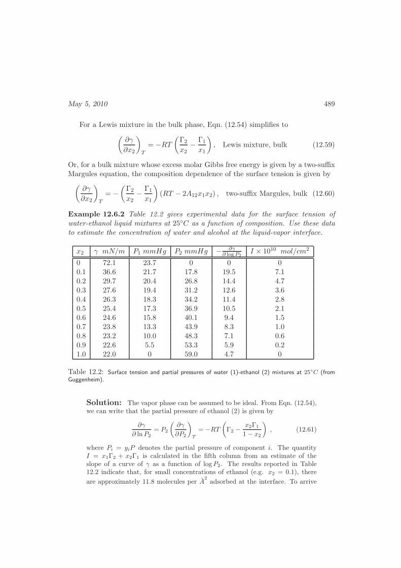
May 5, 2010 489
For a Lewis mixture in the bulk phase, Eqn. (12.54) simplifies to
(∂γ
∂x2
)
T
= −RT(Γ2
x2− Γ1
x1
)
, Lewis mixture, bulk (12.59)
Or, for a bulk mixture whose excess molar Gibbs free energy is given by a two-suffixMargules equation, the composition dependence of the surface tension is given by
(∂γ
∂x2
)
T
= −(Γ2
x2− Γ1
x1
)
(RT − 2A12x1x2) , two-suffix Margules, bulk (12.60)
Example 12.6.2 Table 12.2 gives experimental data for the surface tension ofwater-ethanol liquid mixtures at 25C as a function of composition. Use these datato estimate the concentration of water and alcohol at the liquid-vapor interface.
x2 γ mN/m P1 mmHg P2 mmHg − ∂γ∂ logP2
I × 1010 mol/cm2
0 72.1 23.7 0 0 00.1 36.6 21.7 17.8 19.5 7.10.2 29.7 20.4 26.8 14.4 4.70.3 27.6 19.4 31.2 12.6 3.60.4 26.3 18.3 34.2 11.4 2.80.5 25.4 17.3 36.9 10.5 2.10.6 24.6 15.8 40.1 9.4 1.50.7 23.8 13.3 43.9 8.3 1.00.8 23.2 10.0 48.3 7.1 0.60.9 22.6 5.5 53.3 5.9 0.21.0 22.0 0 59.0 4.7 0
Table 12.2: Surface tension and partial pressures of water (1)-ethanol (2) mixtures at 25C (fromGuggenheim).
Solution: The vapor phase can be assumed to be ideal. From Eqn. (12.54),we can write that the partial pressure of ethanol (2) is given by
∂γ
∂ lnP2= P2
(∂γ
∂P2
)
T
= −RT(
Γ2 −x2Γ1
1− x2
)
, (12.61)
where Pi = yiP denotes the partial pressure of component i. The quantityI = x1Γ2 + x2Γ1 is calculated in the fifth column from an estimate of theslope of a curve of γ as a function of logP2. The results reported in Table12.2 indicate that, for small concentrations of ethanol (e.g. x2 = 0.1), there
are approximately 11.8 molecules per A2adsorbed at the interface. To arrive
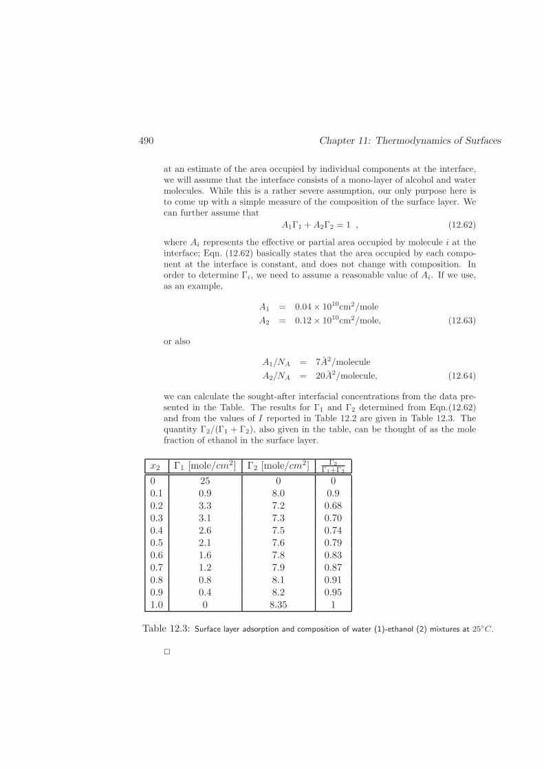
490 Chapter 11: Thermodynamics of Surfaces
at an estimate of the area occupied by individual components at the interface,we will assume that the interface consists of a mono-layer of alcohol and watermolecules. While this is a rather severe assumption, our only purpose here isto come up with a simple measure of the composition of the surface layer. Wecan further assume that
A1Γ1 +A2Γ2 = 1 , (12.62)
where Ai represents the effective or partial area occupied by molecule i at theinterface; Eqn. (12.62) basically states that the area occupied by each compo-nent at the interface is constant, and does not change with composition. Inorder to determine Γi, we need to assume a reasonable value of Ai. If we use,as an example,
A1 = 0.04× 1010cm2/mole
A2 = 0.12× 1010cm2/mole, (12.63)
or also
A1/NA = 7A2/molecule
A2/NA = 20A2/molecule, (12.64)
we can calculate the sought-after interfacial concentrations from the data pre-sented in the Table. The results for Γ1 and Γ2 determined from Eqn.(12.62)and from the values of I reported in Table 12.2 are given in Table 12.3. Thequantity Γ2/(Γ1 + Γ2), also given in the table, can be thought of as the molefraction of ethanol in the surface layer.
x2 Γ1 [mole/cm2] Γ2 [mole/cm2] Γ2Γ1+Γ2
0 25 0 00.1 0.9 8.0 0.90.2 3.3 7.2 0.680.3 3.1 7.3 0.700.4 2.6 7.5 0.740.5 2.1 7.6 0.790.6 1.6 7.8 0.830.7 1.2 7.9 0.870.8 0.8 8.1 0.910.9 0.4 8.2 0.951.0 0 8.35 1
Table 12.3: Surface layer adsorption and composition of water (1)-ethanol (2) mixtures at 25C.
2
May 5, 2010 491
In the previous example, experimental data for the surface tension of binarymixtures of water and ethanol were measured in the laboratory. From those datawe arrived at estimates of the composition of the surface layer which, in general,turned out to be significantly different from that of the bulk liquid. It is generallydesirable to develop methods for prediction of the surface tension of mixtures fromknowledge of those corresponding to the pure components. Such methods mustnecessarily capture the fact that the surface layer’s composition is influenced by thepure component’s surface tensions. Species that exhibit a small surface tension aremore likely to be concentrated in the surface layer; a mixture’s surface tension istherefore generally lower than that corresponding to a simple mole fraction averageof the pure-component surface tensions. Several correlations have been proposedto estimate the surface tension of multicomponent mixtures. Several of these aredescribed in the Exercises at the end of this chapter.
12.6.2 Liquid-Liquid Interfaces
In the particular case of a liquid-liquid interface, the system has only one degreeof freedom and the composition of the interface is completely determined by tem-perature. The derivation of the temperature dependence of γ is analogous to thatpresented earlier for a pure component, and is therefore left as an exercise for thereader.
12.7 Summary
492 Chapter 11: Thermodynamics of Surfaces
12.8 Exercises
12.1.A. Estimate the surface tension of n-hexane at 25C from the heat of vaporiza-tion. You will need to consider the physical picture of an interface introduced in thischapter, and estimate the energy per nearest-neighbor of an individual molecule inthe liquid phase. You will also need to estimate the area occupied by an individualmolecule at the surface. The interfacial tension of n-hexane at 25C is approximately0.0179 N/m; how does your estimate compare with the experimental value?
12.1.B. The surface tension of a liquid can be inferred from the force that a liquidexerts on a plate that is partly submerged, vertically, into the liquid. Show that,provided the liquid “wets” the surface of the plate, a downward force of magnitude2γl is experienced by the plate (l is the length of the plate). This force provides thebasis for the Wilhelmy Plate methods to measure surface tensions.
12.3.A. Consider an air bubble in water at 25C. What is the difference in pressurebetween the interior and exterior of the bubble when the diameter is 1 mm? Whatis that difference for a nano-bubble of diameter 40 nm?
12.3.B. Consider a capillary tube of diameter 0.1 mm. A liquid is allowed to flowout of the capillary, leading to the formation of a drop at its outlet. Show that thecritical radius rc at which the drop will detach from the capillary tube is given by:
rc =mg
2πγ. (12.65)
At room temperature, what is the size that a water droplet will have before itdetaches from the capillary? Equation (12.65) provides the basis for a techniqueto measure the surface tension of liquids. Would there be an advantage to usingsmaller or larger capillary tubes? Please explain.
12.3.C. Consider a bubble of air of diameter r in liquid water. Show that, assumingideal gas behavior, the vapor pressure inside the bubble (P bubble,sat) is lower thanin the bulk liquid by an amount
logP bubble,sat
P b,sat= − 2γv
rRT, (12.66)
where v is the molar volume of liquid water. Calculate the ratio of the vapor pressureinside and outside the bubble, at 25, for bubbles of 10, 100 and 1000 nm. A liquidcan sometimes be heated over its boiling point. When that happens, small bubblesare formed in which the vapor pressure is lower than that of the bulk, leading tocondensation of the vapor and collapse of the bubble. Eqn. (12.66) explains whythe vapor pressure in the bubble is lower.
May 5, 2010 493
12.3.D. Zuo and Stenby (Y.X. Zuo and E.H. Stenby, Can. J. Chem. Eng., 75, 1130(1997)) have proposed the following correlation to estimate the surface tension ofsimple liquids in terms of critical constants. A reduced surface tension is given by
γr = log
(
1 +γ
T1/3c P
2/3c
)
, (12.67)
where γ, Tc and Pc are given in mN/m, K, and bar, respectively. The reducedsurface tension γr for a fluid of interest is related to that of two reference fluids,namely methane ;/(1) and n-octane (2), according to
γr = γ(1)r +ω − ω(1)
ω(2) − ω(1)(γ(2)r − γ(1)r ) . (12.68)
For methane, γ(1) is given by
γ(1) = 40.52(1 − Tr)1.287 , (12.69)
and for n-octane, γ(2) is given by
γ(2) = 52.095(1 − Tr)1.21548 . (12.70)
1. Use the Zuo-Stenby correlation to estimate the surface tension of n-octane at20C. The experimental value is γ = 21.62 mN/m.
2. Use the Zuo-Stenby correlation to estimate the surface tension of dodecane at22C. The experimental value is γ = 25.44 mN/m.
3. Use the Zuo-Stenby correlation to estimate the surface tension of toluene at20C. The experimental value is γ = 28.52 mN/m
4. Use the Zuo-Stenby correlation to estimate the surface tension of phenol at40C. The experimental value is γ = 39.27 mN/m.
Please discuss the accuracy of the correlation.
12.3.E. Sastri and Rao (S.R.S. Sastri and K.K. Rao, Chem. Eng. J., 59, 181 (1995))have proposed the following correlation to estimate the surface tension of hydrogen-bonding liquids in terms of critical constants and the normal boiling temperature.In their approach, the surface tension is given by
γ = KP xc Tyb T
zc
(1− Tr1− Tb,r
)m
, (12.71)
where γ, Tc and Pc are given in mN/m, K, and bar, respectively. The constantsappearing in Eqn.(12.71) are given in the following table:
494 Chapter 11: Thermodynamics of Surfaces
Substance K x y z m
Alcohols 2.28 0.25 0.175 0 0.8Acids 0.125 0.5 -1.5 1.85 11/9All others 0.158 0.5 -1.5 1.85 11/9
Table 12.4: Parameters appearing in the Sastri-Rao correlation for surface tension.
1. Use the Sastri-Rao correlation to estimate the surface tension of n-octane at20C. The experimental value is γ = 21.62 mN/m.
2. Use the Sastri-Rao correlation to estimate the surface tension of toluene at20C. The experimental value is γ = 28.52 mN/m
3. Use the Sastri-Rao correlation to estimate the surface tension of ethanol at30C. The experimental value is γ = 21.55 mN/m
4. Use the Sastri-Rao correlation to estimate the surface tension of acetic acid at20C. The experimental value is γ = 27.59 mN/m
5. Use the Sastri-Rao correlation to estimate the surface tension of phenol at40C. The experimental value is γ = 39.27 mN/m.
Please discuss the accuracy of the correlation.
12.4.A. Consider a porous material which is wetted by water. That material isplaced in humid air (the level of humidity is 80%). At 25C and ambient pressure,what is the smallest size of the pores that can fill up with water? What happenswhen the level of humidity is higher (e.g. 90%)? Explain your results. This exampleprovides the basis to conceive experiments for measurement of porosity of solids.Please explain how such experiments might work, and discuss whether it would beadvantageous to use a liquid or a gas with high or with low surface tension.
12.4.B. A capillary of radius r = 0.55 mm is used to measure the surface tensionof benzene. The density of benzene at 20C is ρ = 0.88 g/cm3. The height of thebenzene on the capillary is h = 1.2 cm. Determine the surface tension of benzene.
12.4.C. What is the capillary rise of water in a tube of radius r = 0.5 cm at 20C?
12.5.A. Show that the surface tension between a liquid and a vapor phase can beexpressed as the difference between the Gibbs free energy of the surface layer, andthe Gibbs free energy that the same layer would have if it exhibited the propertiesof the bulk liquid, i.e.
γ = Gσ,∗ − Γgl . (12.72)
May 5, 2010 495
12.6.1.A. The surface tension of water at 25C increases at a rate of approximately∂γ∂C = 1.8 ×10⁻³ N
m mol upon addition of small amounts of sodium chloride. Estimatethe concentration of a 5 mM aqueous solution of sodium chloride.
12.6.1.B. The surface tension of water at 25C decreases at a rate of approximately∂γ∂C = -40 ×10−3 N
m mol upon addition of small amounts of ethanol. Estimate theconcentration of a 5 mM aqueous solution of ethanol.
12.6.1.C. Table 12.5 provides experimental data for the surface tension of aqueoussolutions of SDS. Based on these data, construct a plot of the surface concentrationof SDS as a function of surfactant concentration. You may assume that a moleculeof SDS occupies approximately 1.4 nm2. At an SDS concentration of approximately10 mM , the surface tension makes an abrupt change. Please discuss the cause forthis change. Tajima et al. (K. Tajima, M. Muramatsu, and T. Sasaki, Bull. Chem.
Concentration mM γ [mN/m]
0.5 69.11.1 682 60.33 54.94 485 45.56 43.98 40.510 39.110.5 38.510.8 38.411 38.312 3713 36.5
Table 12.5: Surface tension of an aqueous solution of SDS at 25C.
Soc. Jpn., 43, 1991 (1970))have measured the excess concentration of SDS at theair-water interface by means of radio labeling. Their results are given in Table 12.6.Are your results consistent with the experimental data in computational cost andstorage. that table? Please discuss your results.
12.6.1.D. Hadden (S.T. Hadden, Hydrocarbon Process Petrol. Refiner, 45, 161(1966)) has proposed the following correlation for the surface tension γm of mix-
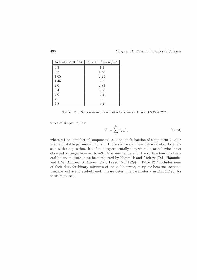
496 Chapter 11: Thermodynamics of Surfaces
Activity ×10−3M Γ2 × 10⁻⁶ mole/m2
0.3 1.10.7 1.651.05 2.251.45 2.52.0 2.832.4 3.053.0 3.24.1 3.24.8 3.2
Table 12.6: Surface excess concentration for aqueous solutions of SDS at 25C.
tures of simple liquids:
γrm =
n∑
i
xiγri , (12.73)
where n is the number of components, xi is the mole fraction of component i, and ris an adjustable parameter. For r = 1, one recovers a linear behavior of surface ten-sion with composition. It is found experimentally that when linear behavior is notobserved, r ranges from −1 to −3. Experimental data for the surface tension of sev-eral binary mixtures have been reported by Hammick and Andrew (D.L. Hammickand L.W. Andrew, J. Chem. Soc., 1929, 754 (1929)). Table 12.7 includes someof their data for binary mixtures of ethanol-benzene, m-xylene-benzene, acetone-benzene and acetic acid-ethanol. Please determine parameter r in Eqn.(12.73) forthese mixtures.
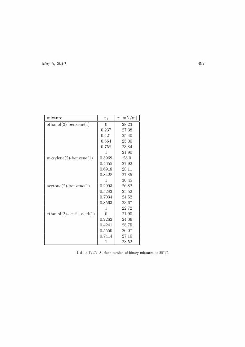
May 5, 2010 497
mixture x1 γ [mN/m]
ethanol(2)-benzene(1) 0 28.230.237 27.380.421 25.400.564 25.000.758 23.841 21.90
m-xylene(2)-benzene(1) 0.3969 28.00.4655 27.920.6918 28.110.8428 27.85
1 30.45acetone(2)-benzene(1) 0.2993 26.82
0.5283 25.520.7034 24.520.8563 23.67
1 22.72ethanol(2)-acetic acid(1) 0 21.90
0.2262 24.060.4241 25.750.5550 26.070.7414 27.10
1 28.52
Table 12.7: Surface tension of binary mixtures at 25C.

498 Appendix
Appendix A
Mathematical Background
In thermodynamics we often switch between different sets of independent variables.For example, we develop the fundamental structure of the subject using internalenergy as the dependent variable whereas entropy, volume and mole numbers are theindependent variables. However, in experiments we often manipulate temperatureand pressure, so that we would like to use T and P as the independent variables.Therefore, it is essential that students of thermodynamics are comfortable with themanipulation of partial differentiation and the conversion between different sets ofindependent variables.
In this appendix we give a summary of all of the mathematical concepts necessaryto perform the manipulations used in this text. As is made clear below, thesemanipulations can be reduced to a minimum number. When the methods describedhere are combined with the strategies discussed in §3.6, any desired simplificationcan be obtained with little effort, memorization, or error.
In what follows, we consider a dependent variable ψ to be a function of indepen-dent variables u, v and w
ψ = ψ(u, v, w) (A.1)
A.1 Taylor’s series expansion
A suitably smooth function of more that one argument may be expanded in aTaylor’s series around the point (u, v, w) as
ψ(u+ du, v + dv,w + dw) = ψ(u, v, w) + dψ +1
2d2ψ + . . . , (A.2)
499

500 Appendix
where we define
dψ :=
(∂ψ
∂u
)
v,w
du+
(∂ψ
∂v
)
u,w
dv +
(∂ψ
∂w
)
u,v
dw (A.3)
d2ψ :=
(∂2ψ
∂u2
)
(du)2 +
(∂2ψ
∂v2
)
(dv)2 +
(∂2ψ
∂w2
)
(dw)2 (A.4)
+2
(∂2ψ
∂u∂v
)
dudv + 2
(∂2ψ
∂v∂w
)
dvdw + 2
(∂2ψ
∂w∂u
)
dwdu.
The variables written as subscripts following the right parentheses in Eqn. (A.3)are those being held constant during differentiation; thus, in the first term on theright side of Eqn. (A.3), we can tell that the independent variables are u, v andw. We have used the notation typical in thermodynamics, whereas the more usual
mathematical notation is(∂ψ∂u
)
v,w≡ ∂
∂uψ(u, v, w). The second order differentials
in Eqn. (A.4) do not have such indications, so when we use them, we need tokeep careful track of what the independent variables are, or perhaps safest is touse the mathematical notation. If ψ is an analytic function, then the order ofdifferentiation is unimportant, and we can write
(∂2ψ
∂u∂v
)
w
=
(∂2ψ
∂v∂u
)
w
. (A.5)
We will assume in this text that all thermodynamic functions are analytic. The firstdifferential Eqn. (A.3) is important for nearly all of thermodynamics, (i.e., in theintegration of energy, or in order to find maxima). The second differential Eqn. (A.4)is important when considering stability criteria.
A.2 The Chain Rule
Sometimes we switch from one set of independent variables, such as energy, volumeand mole number, to another set, such as temperature, pressure and chemical po-tential. Then, we need to find differentials in the new set using what we know aboutthe old set. For example, suppose that we know the relations
u = u(x, y, z)
v = v(x, y, z)
w = w(x, y, z), (A.6)
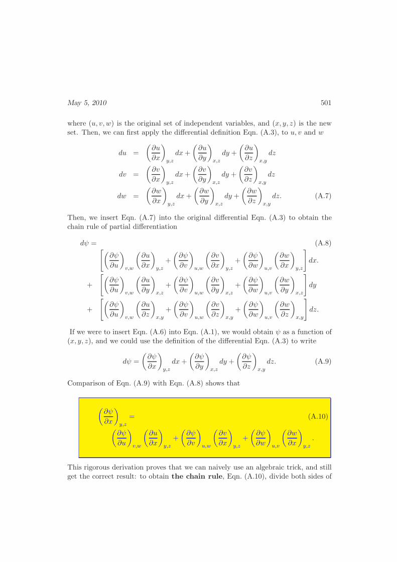
May 5, 2010 501
where (u, v, w) is the original set of independent variables, and (x, y, z) is the newset. Then, we can first apply the differential definition Eqn. (A.3), to u, v and w
du =
(∂u
∂x
)
y,z
dx+
(∂u
∂y
)
x,z
dy +
(∂u
∂z
)
x,y
dz
dv =
(∂v
∂x
)
y,z
dx+
(∂v
∂y
)
x,z
dy +
(∂v
∂z
)
x,y
dz
dw =
(∂w
∂x
)
y,z
dx+
(∂w
∂y
)
x,z
dy +
(∂w
∂z
)
x,y
dz. (A.7)
Then, we insert Eqn. (A.7) into the original differential Eqn. (A.3) to obtain thechain rule of partial differentiation
dψ = (A.8)[(
∂ψ
∂u
)
v,w
(∂u
∂x
)
y,z
+
(∂ψ
∂v
)
u,w
(∂v
∂x
)
y,z
+
(∂ψ
∂w
)
u,v
(∂w
∂x
)
y,z
]
dx.
+
[(∂ψ
∂u
)
v,w
(∂u
∂y
)
x,z
+
(∂ψ
∂v
)
u,w
(∂v
∂y
)
x,z
+
(∂ψ
∂w
)
u,v
(∂w
∂y
)
x,z
]
dy
+
[(∂ψ
∂u
)
v,w
(∂u
∂z
)
x,y
+
(∂ψ
∂v
)
u,w
(∂v
∂z
)
x,y
+
(∂ψ
∂w
)
u,v
(∂w
∂z
)
x,y
]
dz.
If we were to insert Eqn. (A.6) into Eqn. (A.1), we would obtain ψ as a function of(x, y, z), and we could use the definition of the differential Eqn. (A.3) to write
dψ =
(∂ψ
∂x
)
y,z
dx+
(∂ψ
∂y
)
x,z
dy +
(∂ψ
∂z
)
x,y
dz. (A.9)
Comparison of Eqn. (A.9) with Eqn. (A.8) shows that
(∂ψ
∂x
)
y,z
= (A.10)
(∂ψ
∂u
)
v,w
(∂u
∂x
)
y,z
+
(∂ψ
∂v
)
u,w
(∂v
∂x
)
y,z
+
(∂ψ
∂w
)
u,v
(∂w
∂x
)
y,z
.
This rigorous derivation proves that we can naively use an algebraic trick, and stillget the correct result: to obtain the chain rule, Eqn. (A.10), divide both sides of
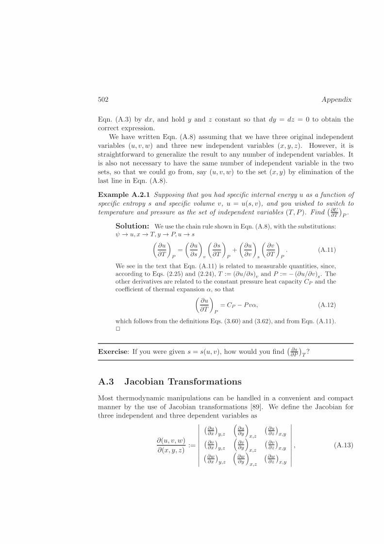
502 Appendix
Eqn. (A.3) by dx, and hold y and z constant so that dy = dz = 0 to obtain thecorrect expression.
We have written Eqn. (A.8) assuming that we have three original independentvariables (u, v, w) and three new independent variables (x, y, z). However, it isstraightforward to generalize the result to any number of independent variables. Itis also not necessary to have the same number of independent variable in the twosets, so that we could go from, say (u, v, w) to the set (x, y) by elimination of thelast line in Eqn. (A.8).
Example A.2.1 Supposing that you had specific internal energy u as a function ofspecific entropy s and specific volume v, u = u(s, v), and you wished to switch totemperature and pressure as the set of independent variables (T, P ). Find
(∂U∂T
)
P.
Solution: We use the chain rule shown in Eqn. (A.8), with the substitutions:ψ → u, x→ T, y → P, u→ s
(∂u
∂T
)
P
=
(∂u
∂s
)
v
(∂s
∂T
)
P
+
(∂u
∂v
)
s
(∂v
∂T
)
P
. (A.11)
We see in the text that Eqn. (A.11) is related to measurable quantities, since,according to Eqs. (2.25) and (2.24), T := (∂u/∂s)v and P := − (∂u/∂v)s. Theother derivatives are related to the constant pressure heat capacity CP and thecoefficient of thermal expansion α, so that
(∂u
∂T
)
P
= CP − Pvα, (A.12)
which follows from the definitions Eqs. (3.60) and (3.62), and from Eqn. (A.11).2
Exercise: If you were given s = s(u, v), how would you find(∂s∂P
)
T?
A.3 Jacobian Transformations
Most thermodynamic manipulations can be handled in a convenient and compactmanner by the use of Jacobian transformations [89]. We define the Jacobian forthree independent and three dependent variables as
∂(u, v, w)
∂(x, y, z):=
∣∣∣∣∣∣∣∣∣∣
(∂u∂x
)
y,z
(∂u∂y
)
x,z
(∂u∂z
)
x,y(∂v∂x
)
y,z
(∂v∂y
)
x,z
(∂v∂z
)
x,y(∂w∂x
)
y,z
(∂w∂y
)
x,z
(∂w∂z
)
x,y
∣∣∣∣∣∣∣∣∣∣
, (A.13)
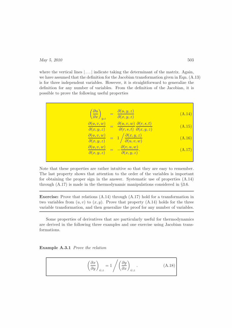
May 5, 2010 503
where the vertical lines | . . . | indicate taking the determinant of the matrix. Again,we have assumed that the definition for the Jacobian transformation given in Eqn. (A.13)is for three independent variables. However, it is straightforward to generalize thedefinition for any number of variables. From the definition of the Jacobian, it ispossible to prove the following useful properties
(∂u
∂x
)
y,z
=∂(u, y, z)
∂(x, y, z)(A.14)
∂(u, v, w)
∂(x, y, z)=
∂(u, v, w)
∂(r, s, t)
∂(r, s, t)
∂(x, y, z)(A.15)
∂(u, v, w)
∂(x, y, z)= 1
/∂(x, y, z)
∂(u, v, w)(A.16)
∂(u, v, w)
∂(x, y, z)= −∂(v, u,w)
∂(x, y, z). (A.17)
Note that these properties are rather intuitive so that they are easy to remember.The last property shows that attention to the order of the variables is importantfor obtaining the proper sign in the answer. Systematic use of properties (A.14)through (A.17) is made in the thermodynamic manipulations considered in §3.6.
Exercise: Prove that relations (A.14) through (A.17) hold for a transformation intwo variables from (u, v) to (x, y). Prove that property (A.14) holds for the threevariable transformation, and then generalize the proof for any number of variables.
Some properties of derivatives that are particularly useful for thermodynamicsare derived in the following three examples and one exercise using Jacobian trans-formations.
Example A.3.1 Prove the relation
(∂x
∂y
)
ψ,z
= 1
/(∂y
∂x
)
ψ,z
. (A.18)
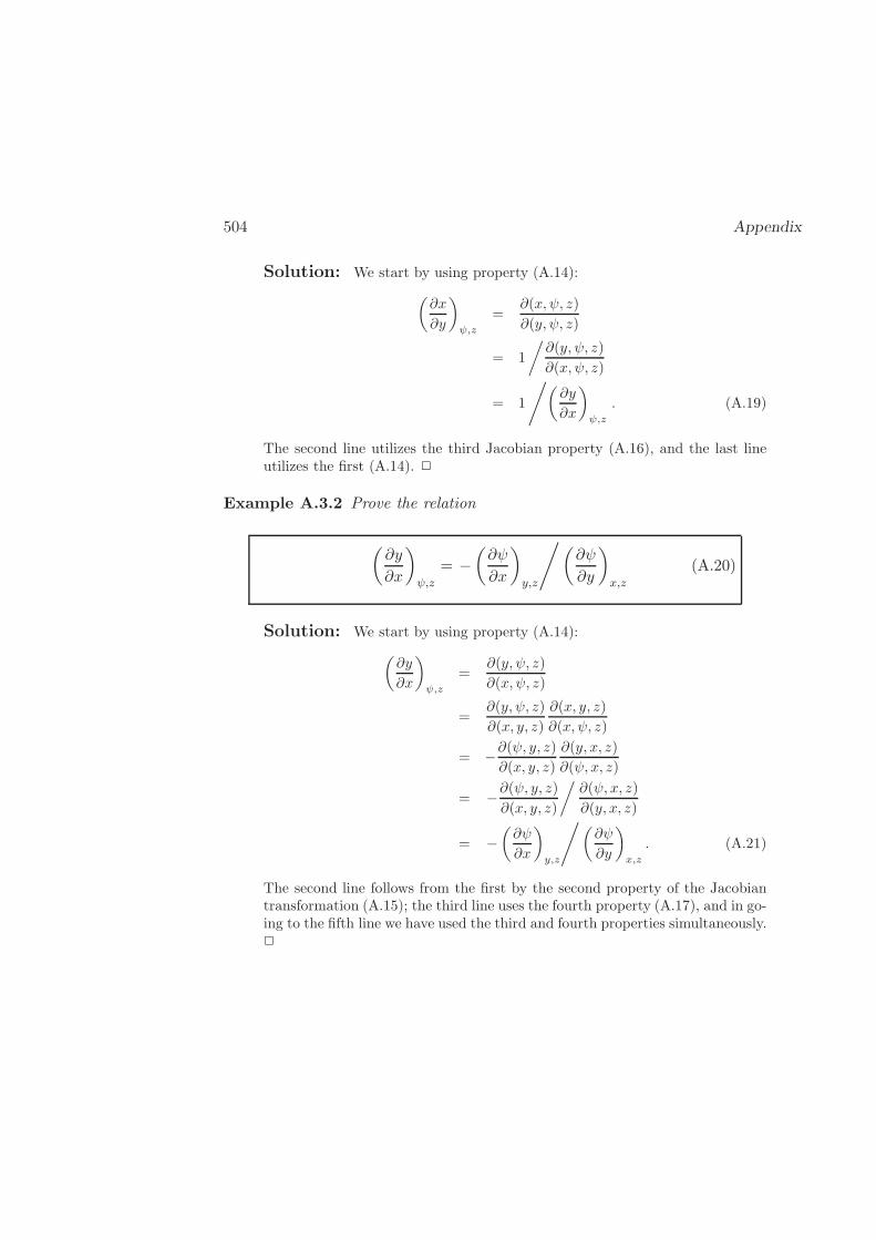
504 Appendix
Solution: We start by using property (A.14):
(∂x
∂y
)
ψ,z
=∂(x, ψ, z)
∂(y, ψ, z)
= 1
/∂(y, ψ, z)
∂(x, ψ, z)
= 1
/(∂y
∂x
)
ψ,z
. (A.19)
The second line utilizes the third Jacobian property (A.16), and the last lineutilizes the first (A.14). 2
Example A.3.2 Prove the relation
(∂y
∂x
)
ψ,z
= −(∂ψ
∂x
)
y,z
/(∂ψ
∂y
)
x,z
(A.20)
Solution: We start by using property (A.14):
(∂y
∂x
)
ψ,z
=∂(y, ψ, z)
∂(x, ψ, z)
=∂(y, ψ, z)
∂(x, y, z)
∂(x, y, z)
∂(x, ψ, z)
= −∂(ψ, y, z)∂(x, y, z)
∂(y, x, z)
∂(ψ, x, z)
= −∂(ψ, y, z)∂(x, y, z)
/∂(ψ, x, z)
∂(y, x, z)
= −(∂ψ
∂x
)
y,z
/(∂ψ
∂y
)
x,z
. (A.21)
The second line follows from the first by the second property of the Jacobiantransformation (A.15); the third line uses the fourth property (A.17), and in go-ing to the fifth line we have used the third and fourth properties simultaneously.2
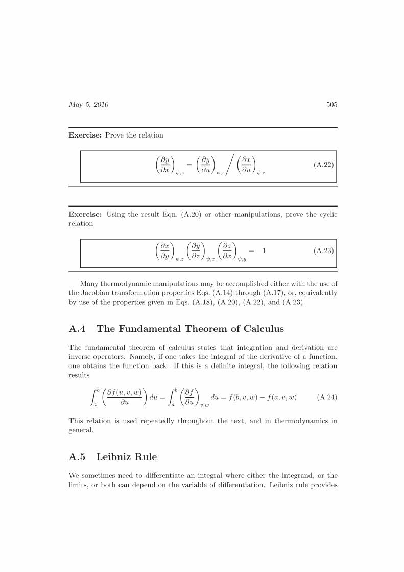
May 5, 2010 505
Exercise: Prove the relation
(∂y
∂x
)
ψ,z
=
(∂y
∂u
)
ψ,z
/(∂x
∂u
)
ψ,z
(A.22)
Exercise: Using the result Eqn. (A.20) or other manipulations, prove the cyclicrelation
(∂x
∂y
)
ψ,z
(∂y
∂z
)
ψ,x
(∂z
∂x
)
ψ,y
= −1 (A.23)
Many thermodynamic manipulations may be accomplished either with the use ofthe Jacobian transformation properties Eqs. (A.14) through (A.17), or, equivalentlyby use of the properties given in Eqs. (A.18), (A.20), (A.22), and (A.23).
A.4 The Fundamental Theorem of Calculus
The fundamental theorem of calculus states that integration and derivation areinverse operators. Namely, if one takes the integral of the derivative of a function,one obtains the function back. If this is a definite integral, the following relationresults
∫ b
a
(∂f(u, v, w)
∂u
)
du =
∫ b
a
(∂f
∂u
)
v,w
du = f(b, v, w) − f(a, v, w) (A.24)
This relation is used repeatedly throughout the text, and in thermodynamics ingeneral.
A.5 Leibniz Rule
We sometimes need to differentiate an integral where either the integrand, or thelimits, or both can depend on the variable of differentiation. Leibniz rule provides
506 Appendix
the means to evaluate such a differentiation
∂
∂u
∫ B(u,w)
A(u,w)ψ(u, v, w)dv =
∫ B(u,w)
A(u,w)
∂ψ(u, v, w)
∂udv − (A.25)
(∂A
∂u
)
w
ψ(u,A(u,w), w) +
(∂B
∂u
)
w
ψ(u,B(u,w), w).
Example A.5.1 Find the derivative with respect to x of the integral
∫ x2
0sin(xy) exp
(−y2
)dy (A.26)
Solution: We just use Leibniz formula, Eqn. (A.25), with the substitutions(u→ x, v → y, w → 0, ψ → sin(xy) exp
(−y2
))
∂
∂x
∫ x2
0
sin(xy) exp(−y2
)dy (A.27)
=
∫ x2
0
∂
∂x
[sin(xy) exp
(−y2
)]dy + 2x sin(xy) exp
(−y2
)∣∣y=x2
=
∫ x2
0
y cos(xy) exp(−y2
)dy + 2x sin(x3) exp
(−x4
).
2
There is a generalization of the Leibniz formula for derivatives of volume integralswhose boundaries may be time dependent
d
dt
∫∫∫
V (t)
(. . .)dV =
∫∫∫
V (t)
∂
∂t(. . .)dV +
∫∫
A(t)
(. . .)(~n · ~vA)dA, (A.28)
where ~vA is the velocity of the moving boundary at dA. This formula is usedimplicitly in only one location in this book, §5.1, and is not essential material. Theformula is sometimes also called Reynolds Transport Theorem.
A.6 Gauss Divergence Theorem
The Gauss divergence theorem yields an equivalence between the volume integral ofthe divergence of a vector field ~ψ, and a surface integral
∫∫∫
V (t)
∇ · ~ψ(~r, t)dV =
∫∫
A(t)
~n · ~ψ(~r, t)dA (A.29)
May 5, 2010 507
where A represents the whole surface of the volume, V is the enclosed volume, ~nis the unit outward normal vector of the surface element dA. This equation is alsoused only in §5.1, and is not essential.
A.7 Solutions to cubic equations
In order to predict phase changes in fluids, equations of state must predict a de-pendence on volume that is cubic, or higher. Hence, many equations of state arecubic, and methods for inverting cubic equations are helpful for studying stability.We first write our cubic equation for x in the form
x3 + a2x2 + a1x+ a0 = 0. (A.30)
The equation may have 1, 2 or 3 roots; we are interested only when there existeither 1 or 3 roots [1]. We can determine the number of roots from the sign of thediscriminant q3 + r2 where
q :=3a1 − a22
9
r :=a2(9a1 − 2a22
)− 27a0
54. (A.31)
When q3 + r2 > 0 there is a single real root to Eqn. (A.30)
x1 =(
r +√
q3 + r2)1/3
+(
r −√
q3 + r2)1/3
− a23. (A.32)
When q3 + r2 < 0, then Eqn. (A.30) has three real roots
x1 = 2√−q cos
(θ
3
)
− a23
x2 = −2√−q cos
(θ − π
3
)
− a23
x3 = −2√−q cos
(θ + π
3
)
− a23, (A.33)
where
θ := cos−1
(
r√
−q3
)
. (A.34)
These equations are particularly useful for programming, for example. Table A.1gives the coefficients necessary to find v = v(T, P ) for several cubic equations ofstate.
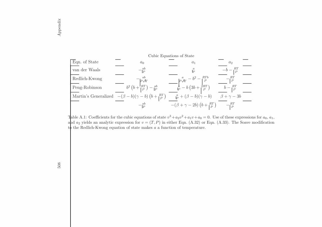
508
Appen
dix
Cubic Equations of State
Eqn. of State a0 a1 a2
van der Waals −abP
aP
−b− RTP
Redlich-Kwong − abP√T
aP√T− b2 − RTb
P−RT
P
Peng-Robinson b2(b+ RT
P
)− ab
PaP− b
(3b+ 2RT
P
)b− RT
P
Martin’s Generalized −(β − b)(γ − b)(b+ RT
P
)aP+ (β − b)(γ − b) β + γ − 3b
−abP
−(β + γ − 2b)(b+ RT
P
)−RT
P
Table A.1: Coefficients for the cubic equations of state v3+a2v2+a1v+a0 = 0. Use of these expressions for a0, a1,
and a2 yields an analytic expression for v = (T, P ) in either Eqn. (A.32) or Eqn. (A.33). The Soave modificationto the Redlich-Kwong equation of state makes a a function of temperature.
May 5, 2010 509
A.8 Combinatorics
In statistical mechanics we often have to count large numbers of possible configura-tions of molecules in order to find the partition function. Many of these problemsare isomorphic to the urn problems of probability. Here we summarize the problemof arranging many indistinguishable objects in distinguishable locations. We firstuse the binomial theorem for two such objects, and then generalize to an arbitrarynumber.
A.8.1 Binomial Theorem
How many ways can you arrange Nw (indistinguishable) white marbles, and Nb
(indistinguishable) black marbles in Nw +Nb (distinguishable) boxes? This can befound in two steps:
1. Pick the marbles blindly, one at a time, out of a bag and fill the boxes in order.The first box has (Nw +Nb) possibilities. The second box has (Nw +Nb− 1),since you have removed one marble from the bag to fill the first box. Keepdoing this until the bag is empty. The total number of such possibilities is theproduct of the number of possibilities of each box:
(Nw +Nb)(Nw +Nb − 1) · · · 1 = (Nw +Nb)!.
2. Since the white marbles are indistinguishable, we have over-counted thesepossibilities—some arrangements we have created in the first step are redun-dant. Let us count these redundancies. Take a given arrangement created inthe first step, and remove all the white marbles from their boxes and returnthem to the bag. Now do like we did before, but with just the white marblesand the empty boxes. How many different ways can we put them back?
Nw(Nw − 1) · · · 1 = Nw!.
Note that this result did not depend on what our chosen arrangement lookslike: the same answer applies to all arrangements. We can do the same step forthe black marbles. Hence, we have counted each unique arrangement Nw!Nb!times in the first step.
Hence, we get that there are
(Nw +Nb
Nw
)
:=(Nw +Nb)!
Nw!Nb!

510 Appendix
unique ways to arrange these white and black marbles, in answer to our first question.The term on the left side is called the binomial coefficient, since it arises in
expanding powers of a sum of two terms [1, §3.1]
(a+ b)n =n∑
i=0
(ni
)
an−ibi
For the Langmuir adsorption isotherm example, sites with a molecule adsorbedare white, and desorbed are black, so Nw = NNA and Nw+Nb =MsNA, where NA
is Avogadro’s number.
A.8.2 Multinomial Theorem
Now generalize the binomial problem to having more than two kinds of marbles.Let’s make them billiard balls with numbers painted on them. We have N1 ballswith the number 1, N2 with number 2, etc. Then, the total number of arrangementsin step 1 is (
∑mi=1Ni)!, where there are m different kinds of balls.
Again we have over-counted. Step two generalized leads to N1!N2! . . . Nm! over-counts. Hence, the total number of unique ways to arrange the balls is
(
r∑
i=1
Ni;N1, N2, . . . , Nr) :=(∑r
i=1Ni)!
N1!N2! . . . Nr!.
This is called the multinomial coefficient, since [1, §24.1.1]
(x1+x2+. . .+xr)n =
∑
N1
∑
N2
. . .∑
Nr
(n;N1, N2, . . . , Nr)δ
(
n,
r∑
i=1
Ni
)
xN11 xN2
2 . . . xNrm
where we used the delta function: δ(i, j) = 1 only if i = j. This keeps therestriction that the sums must keep
∑ri=1Ni = n. Or, we can write the above in
shorthand(
r∑
i=1
xi
)n
=∑
~N
(n;N1, N2, . . . , Nr)δ
(
n,
r∑
i=1
Ni
)r∏
i=1
xNii
=∑
~N
n!δ
(
n,
r∑
i=1
Ni
)r∏
i=1
xNiiNi!
. (A.35)
The application of this result to the B.E.T. theory (see Exercise 3.7.E.), forexample, is straightforward.
May 5, 2010 511
Exercise Write down explicitly the probability that ‘heads’ appears n times afterN coin tosses. Find the most probable value for n.
Exercise. There are two boxes with volumes V1, and V2 which communicate by ahole that allows molecules to pass through. There are N1 molecules of species 1,and N2 molecules of species 2 distributed between the two boxes. Assuming thatthe probability for a molecule to be in a box is proportional to the volume of thebox, find the probability that there are n1 molecules of species 1 in box 1, and n2molecules of species 2 in box 1.
Exercise. A poker hand is five cards drawn randomly from a deck of 52 cards. Howmany different hands are possible? Make your derivation of the answer clear.
Exercise. Suppose that a strand of DNA contains 100 base pairs. If there arean equal number of each kind of base pair, how many different combinations arepossible?

512 Appendix
Appendix B
Fluid Equations of State
The text considers the ideal gas and van der Waals equations of state in somedetail. In addition to these, we summarize here several more-accurate equations ofstate. This appendix represents but a small fraction of such equations. A morecomprehensive discussion of the quality of such equations is made in [86].
Note that all fluid equations of state reduce to the general ideal gas at lowdensities. For small deviations away from ideal behavior, the virial expansion is themost reliable. However, it is not appropriate for predicting vapor-liquid equilibria.The cubic equations of state are straightforward to use and computationally simple.However, some sacrifice must be made for accuracy. Of these, the Peng-Robinson,Soave-Redlich-Kwong and Schmidt-Wenzel equations are usually superior. However,all cubic equations are suspect near the critical region. For an excellent reviewof many such equations, see [2]. If computational ease should be sacrificed foraccuracy, the Benedict-Webb-Rubin and the Anderko-Pitzer equations are usuallymore accurate.
The parameters in the cubic PV T equations of state are usually determinedfrom the critical properties of a fluid, and these equations are given. Critical valuesfor a few substances are given in Table D.3. More values can be found from theNIST web page. If the critical values of a substance are not known, they may beestimated from group methods based on the chemical structure of the substance.These methods are reviewed in [71]. The additional parameters necessary for themore-accurate equations are usually of a general nature, and these are also tabulatedin Tables B.3 and B.4. However, if specific values for a substance are known, theseshould, of course, be used instead of the general values.
As an indication of the quality of the equations given here, Table B.1 comparesthe ability of a few equations to describe the vapor and liquid properties of saturatedpropane at 300K.
513
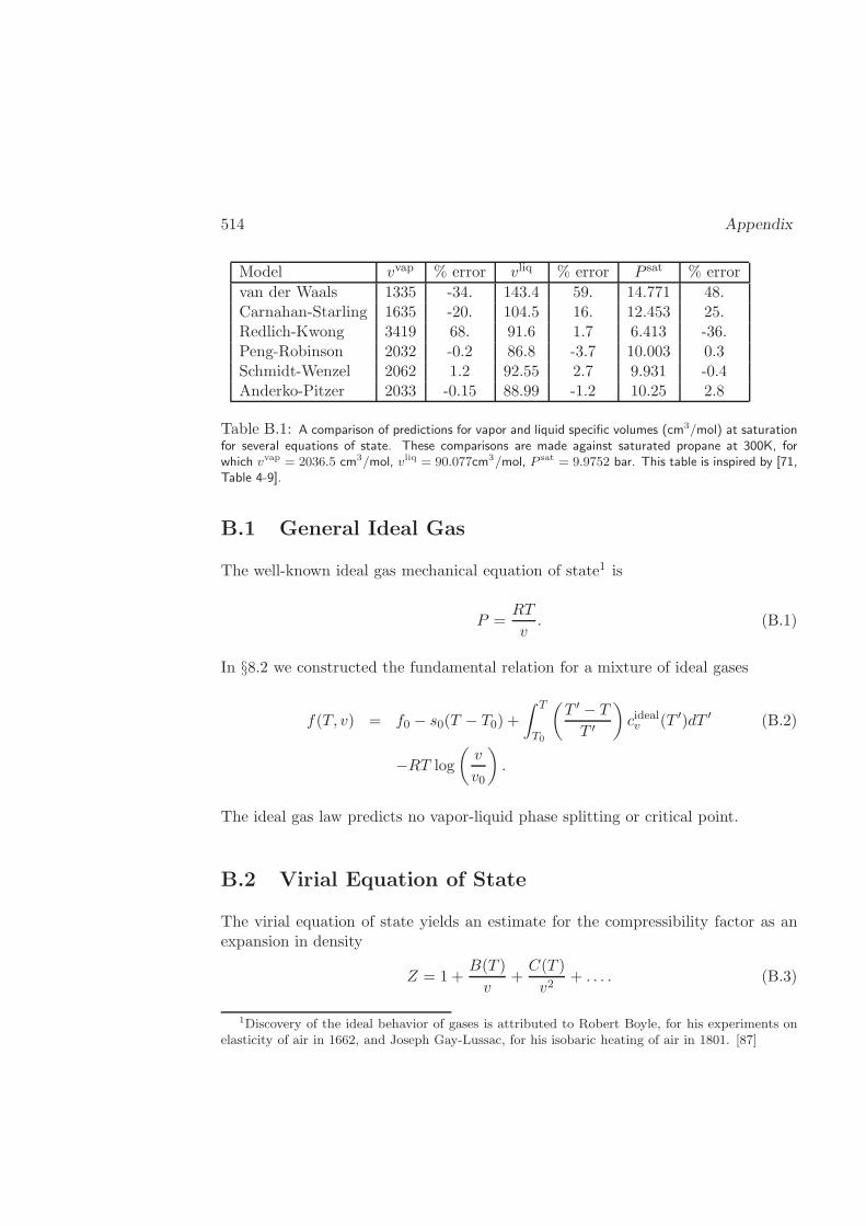
514 Appendix
Model vvap % error vliq % error P sat % error
van der Waals 1335 -34. 143.4 59. 14.771 48.Carnahan-Starling 1635 -20. 104.5 16. 12.453 25.Redlich-Kwong 3419 68. 91.6 1.7 6.413 -36.Peng-Robinson 2032 -0.2 86.8 -3.7 10.003 0.3Schmidt-Wenzel 2062 1.2 92.55 2.7 9.931 -0.4Anderko-Pitzer 2033 -0.15 88.99 -1.2 10.25 2.8
Table B.1: A comparison of predictions for vapor and liquid specific volumes (cm3/mol) at saturationfor several equations of state. These comparisons are made against saturated propane at 300K, forwhich vvap = 2036.5 cm3/mol, vliq = 90.077cm3/mol, P sat = 9.9752 bar. This table is inspired by [71,Table 4-9].
B.1 General Ideal Gas
The well-known ideal gas mechanical equation of state1 is
P =RT
v. (B.1)
In §8.2 we constructed the fundamental relation for a mixture of ideal gases
f(T, v) = f0 − s0(T − T0) +
∫ T
T0
(T ′ − T
T ′
)
cidealv (T ′)dT ′ (B.2)
−RT log
(v
v0
)
.
The ideal gas law predicts no vapor-liquid phase splitting or critical point.
B.2 Virial Equation of State
The virial equation of state yields an estimate for the compressibility factor as anexpansion in density
Z = 1 +B(T )
v+C(T )
v2+ . . . . (B.3)
1Discovery of the ideal behavior of gases is attributed to Robert Boyle, for his experiments onelasticity of air in 1662, and Joseph Gay-Lussac, for his isobaric heating of air in 1801. [87]
May 5, 2010 515
Schreiber and Pitzer2 recommend using a corresponding-states expression for thefirst virial coefficient
Br(Tr) :=B(T )Pc
RTcz∗cz∗c := 0.2905 − 0.0787ω
(B.4)
where Br is found from
Br(Tr) = B0(Tr) + ωB1(Tr)
B0(Tr) = 0.442259 − 0.980970
Tr− 0.611142
T 2r
− 0.00515624
T 6r
B1(Tr) = 0.725650 +0.218714
Tr− 1.24976
T 2r
− 0.189187
T 6r
(B.5)
More recently, Tsonopoulos [100] proposed modifications that apply to polar gasesand associating fluids. For non-associating, and non-polar gases, Tsonopoulos rec-ommends
B(T )Pc
RTc= B0(Tr) + ωB1(Tr)
B0(Tr) = 0.1445 − 0.3300
Tr− 0.1385
T 2r
− 0.0121
T 3r
− 0.000607
T 8r
B1(Tr) = 0.0637 +0.331
T 2r
− 0.423
T 3r
− 0.0008
T 8r
(B.6)
The acentric factor was first introduced by Pitzer, and is found from the behaviorof the fluid at a single point on the PV diagram. Namely,
ω := log10
(Pc
P sat(Tr = 0.7)
)
− 1. (B.7)
Values for ω are tabulated for many substances in Appendix D.One additional term each is necessary to describe polar and associating fluids.
The coefficients, however, are not universal.A correlation for the third term, recommended by Orbey and Vera [100] is
C(T )
(Pc
RTc
)2
= C0(Tr) + ωC1(Tr)
C0(Tr) = 0.01407 +0.02432
T 2.8r
− 0.00313
T 10.5r
C1(Tr) = −0.02676 +0.0177
T 2.8r
+0.040
T 3r
− 0.003
T 6r
− 0.00228
T 10.5r
(B.8)
2[69], p.141.
516 Appendix
These correlations are also for non-polar, non-associating fluids.Experimentally determined values for the coefficients may be found in [24].This equation of state has fundamental relation
f(T, v) = f0 − s0(T − T0) +RT log (v/v0) +
∫ T
T0
(T ′ − T
T ′
)
cidealv (T ′)dT ′ −
RTB(T )
[1
v− 1
v0
]
− 1
2RTC(T )
[1
v2− 1
v20
]
+ . . . , (B.9)
as found from the techniques in §4.4.1. The residual internal energy and Helmholtzpotential are
UR
NRT=
T
v
dB
dT+
T
2v2dC
dT+ . . . , (B.10)
FR
NRT=
B(T )
v+C(T )
2v2+ . . .− log
(
1 +B(T )
v+C(T )
v2+ . . .
)
. (B.11)
The other residual properties can be found from these two. The fugacity is
fpure(T, v) =RT
vexp
[2B(T )
v+
3C(T )
2v2+ . . .
]
, virial expansion (B.12)
There also exist virial expansions in pressure
Z = 1 +B′(T )P +C ′(T )P 2 + . . . , (B.13)
which has fundamental relation
g(T, P ) = g0 − (T − T0)s0 +
∫ T
T0
(T ′ − T
T ′
)
cidealP (T ′)dT ′ +
RT log
(P
P0
)
+B′(T )RTP +1
2C ′(T )RTP 2 + . . . . (B.14)
B.3 Van der Waals Fluid
The van der Waals fluid3 has mechanical equation of state
P =RT
v − b− a
v2. (B.15)
3The van der Waals equation of state plays a key role in the history of thermodynamics. Thereis a recent biography on the life of Johannes Diderik van der Waals (1837-1923) [52], and a detailedhistory of the science surrounding the developments of thermodynamics in the Netherlands aroundthis time [87], in which van der Waals plays a central role. Van der Waals’ doctoral thesis of 1873has also been translated into English [102].
May 5, 2010 517
In §4.4.1 we constructed the fundamental relation
f = f0 − s0(T − T0)−RT log
(v − b
v0 − b
)
− a
(1
v− 1
v0
)
+
∫ T
T0
(T ′ − T
T ′
)
cidealv (T ′)dT ′. (B.16)
The parameters can be found from the predicted critical state
a =27R2T 2
c
64Pc(B.17)
b =RTc8Pc
. (B.18)
The van der Waals fluid predicts a compressibility factor at the critical point ofzc = 3/8, which is typically larger than experiment.
We can use Eqs. (4.75) and (4.76) to find the residual properties predicted bythis model
FR
NRT= −a
v−RT log
[
1− a(v − b)
RTv2
]
, (B.19)
UR
NRT= −a
v, (B.20)
GR
NRT= −2a
v−RT log
[
1− a(v − b)
RTv2
]
+bRT
v − b, (B.21)
HR
NRT=
bRT
v − b− 2a
v, (B.22)
SR
NRT= R log
[
1− a(v − b)
RTv2
]
. (B.23)
The van der Waals model predicts the fugacity expression
fpure(T, v) =RT
v − bexp
[b
v − b− 2a
RTv
]
, van der Waals (B.24)
Using stability analysis as shown in §4.2.2, this model can predict saturationpressure, liquid density and vapor density as functions of sub-critical temperature.We can make an empirical fit to these numerical results of the form
log
(P sat[Tr]
Pc
)
= B(1− Tr) +C(1− Tr)2 +D(1− Tr)
3, (B.25)
where the van der Waals model predicts B = −4.08121, C = −2.04625, D =−7.41366, and the result is valid for reduced temperatures between 0.625 and 1.
518 Appendix
B.4 Carnahan-Starling Equation of State
Carnahan and Starling recommended the following modification to the van derWaalsequation of state
P =RT
v
[v3 + bv2 + b2v − b3
(v − b)3
]
− a
v2, (B.26)
Using the techniques of §4.4.1, we find the corresponding fundamental Helmholtzrelation to be
f = f0 − s0(T − T0) +RT
log(v0v
)
+ b
[4v − 3b
(v − b)2− 4
v0
]
− (B.27)
a
(1
v− 1
v0
)
+
∫ T
T0
(T ′ − T
T ′
)
cidealv (T ′)dT ′.
The parameters for the Carnahan-Starling-van der Waals equation of state can befound from
a ∼= 0.4963877(RTc)
2
Pc
b ∼= 0.0468236RTcPc
. (B.28)
These expressions are found from inverting the results of Problem 4.2.I. The PV Trelation yields a critical compressibility of 0.359, which is too large for most fluids.
We can use Eqs. (4.75) and (4.76) to find the residual properties predicted bythis model
FR
NRT=
bRT (4v − 3b)
(v − b)2−RT log
[v3 + v2b+ vb2 − b3
(v − b)3− a
RTv
]
− a
v(B.29)
UR
NRT= −a
v(B.30)
The other residual properties can be found from these two. The Carnahan-Starlingmodel predicts the fugacity expression
fpure(T, v) =RT
vexp
[
−b(8v2 − 9vb+ 3b2
)
(v − b)3− 2a
RTv
]
, (B.31)
Using stability analysis as shown in §4.2.2, this model can predict saturationpressure, liquid density and vapor density as functions of sub-critical temperature.We can make an empirical fit to these numerical results of the form
log
(P sat[Tr]
Pc
)
= B(1− Tr) + C(1− Tr)2 +D(1− Tr)
3, (B.32)
May 5, 2010 519
where the Carnahan-Starling model predicts B = −4.99803, C = −2.54547, D =−13.2049, and the result is valid for reduced temperatures between 0.635 and 1.
B.5 Redlich-Kwong Equation of State
The Redlich-Kwong equation of state [76] is given by
P =RT
v − b− a√
Tv(v + b). (B.33)
If we use manipulations analogous to those used for the van der Waals fluid in §4.4.1,we find the corresponding fundamental Helmholtz relation for a Redlich-Kwong fluidto be
f = f0 − s0(T − T0)−RT log
(v − b
v0
)
+a
b√T
log
(v
v + b
)
+
∫ T
T0
(T ′ − T
T ′
)
cidealv (T ′)dT ′. (B.34)
The Redlich-Kwong fluid has one of the same shortcomings as the van der Waalsfluid; namely, it predicts a universal value for the critical compressibility factor zc.
Soave [93] has made a modification to this expression, which greatly improvesagreement with data. He recommends allowing the parameter a to depend upontemperature
a(Tr) = a0
[
1 +(
1−√
Tr
)(
m+n
Tr
)]
, (B.35)
wherem and n are material parameters to be estimated from the temperature of thematerial at two different vapor pressures, 10 and 760mm.Hg. He describes severalprocedures to obtain m and n in his paper.
A simpler approximation is
a(Tr) = a0
[
1 + kS
(
1−√
Tr
)]2, (B.36)
where kS depends upon the acentric factor ω
kS = 0.480 + 1.574ω − 0.176ω2, (B.37)
which is a function of the material only (see Eqn. (B.7)). The remaining parameterscan be found from the predicted critical state
a0 ≈ 0.4274804R2T
5/2c
Pc(B.38)
b ≈ 0.0866404RTcPc
. (B.39)
520 Appendix
Both the RK and RKS fluids predict that the critical compressibility is approxi-mately 0.333 (see Problem 4.2.D).
We can use Eqs. (4.75) and (4.76) to find the residual properties predicted bythis model
FR
NRT=
a(T )
b√T
log
(v
v + b
)
−RT log
[
1− (v − b)a(T )
vRT 3/2
]
(B.40)
UR
NRT=
3a(T )− 2Ta′(T )
2b√T
log
(v
v + b
)
(B.41)
The other residual properties can be found from these two. Note that a′(T ) :=da/dT .
The residual Gibbs free energy expression can be inserted into the definition forthe fugacity, Eqn. (8.41) to obtain
fpure(T, v) =RT
v − b
[
RT 3/2v(v + b)− (v − b)a(T )
(v + b)(RT 3/2v − (v − b)a(T )
)
] [v
v + b
] a(T )
bRT3/2
×
exp
[b
v − b− a(T )
RT 3/2(v + b)
]
, Soave-Redlich-Kwong (B.42)
Using stability analysis as shown in §4.2.2, this model can predict saturationpressure, liquid density and vapor density as functions of sub-critical temperature.We can make an empirical fit to these numerical results of the form
log
(P sat[Tr]
Pc
)
= B(1− Tr) + C(1− Tr)2 +D(1− Tr)
3, (B.43)
where the Soave-Redlich-Kwong model predicts
B = −7.18514 − 5.02733ω + 0.453954ω2 , (B.44)
C = −5.04757 − 3.08097ω + 1.36384ω2 ,
D = −23.3129 − 35.5658ω − 11.7846ω2 .
The fit to the model’s prediction is valid for 0.71 ≤ Tr ≤ 1 and −0.3 ≤ ω ≤ 0.3.
B.6 Peng-Robinson Equation of State
The Peng-Robinson PV T relation may be written
P =RT
v − b− a(T )
v(v + b) + b(v − b), (B.45)
May 5, 2010 521
where a has a similar temperature dependence to that used in the Soave modification
a(Tr) = a0
[
1 + kPR
(
1−√
Tr
)]2, (B.46)
and where kPR is
kPR = 0.37464 + 1.54226ω − 0.26992ω2. (B.47)
We find the corresponding fundamental Helmholtz relation for the Peng-Robinsonfluid to be
f = f0 − s0(T − T0)−RT log
(v − b
v0
)
−
a(T )
2√2b
log
[
v + b(1 +√2)
v + b(1−√2)
]
+
∫ T
T0
(T ′ − T
T ′
)
cidealv (T ′)dT ′. (B.48)
using the techniques in §4.4.1. The parameters can be found from the predictedcritical state
a0 ≈ 0.4572367(RTc)
2
Pc(B.49)
b ≈ 0.077796RTcPc
. (B.50)
The critical compressibility factor is predicted by this equation of state to be
zc ≈ 0.307402, (B.51)
which is an improvement over the Soave-Redlich-Kwong prediction, although stilltoo large for many fluids.
We can use Eqs. (4.75) and (4.76) to find the residual properties predicted bythis model
FR
NRT=
a(T )
2√2b
log
[
v −(√
2− 1)b
v +(√
2 + 1)b
]
−RT log
[
1− a(T )(v − b)
RT (v2 + 2vb− b2)
]
(B.52)
UR
NRT=
a(T )− T(da(T )dT
)
2√2b
log
[
v −(√
2− 1)b
v +(√
2 + 1)b
]
(B.53)
522 Appendix
Note that a′(T ) := da/dT . The other residual properties can be found from thesetwo. In particular, the residual Gibbs free energy can be used to express the pure-state fugacity, Eqn. (8.41)
fpure(T, v) =
(RT
v − b
)
exp
[b
v − b− va(T )
RT (v2 + 2vb− b2)
]
×[
v −(√
2− 1)b
v +(√
2 + 1)b
] a(T )
2√
2bRT
(B.54)
Using stability analysis as shown in §4.2.2, this model can predict saturationpressure, liquid density and vapor density as functions of sub-critical temperature.We can make an empirical fit to these numerical results of the form
log
(P sat[Tr]
Pc
)
= B(1− Tr) + C(1− Tr)2 +D(1− Tr)
3, (B.55)
where the Peng-Robinson model predicts
B = −5.72714 − 5.39778ω + 0.820206ω2 , (B.56)
C = −2.73259 − 1.66406ω + 1.50336ω2 ,
D = −12.3843 − 22.7863ω − 9.01297ω2 .
The fit for this model is valid for 0.65 ≤ Tr ≤ 1 and −0.3 ≤ ω ≤ 0.3.
B.7 Martin’s Generalized Cubic Equation of State
Many cubic equations of state can be written in the general form
P =RT
v − b− a(T )
(v + β − b)(v + γ − b)(B.57)
We find the corresponding fundamental Helmholtz relation to be
f = f0 − s0(T − T0)−RT log
(v − b
v0
)
− (B.58)
a(T )
γ − βlog
(v + β − b
v + γ − b
)
+
∫ T
T0
(T ′ − T
T ′
)
cidealv (T ′)dT ′.
from the construction method illustrated in §4.4.1.
May 5, 2010 523
Martin’s generalized cubic equation yields the following predictions for criticalproperties of a fluid
vc = b+(βγ2
)1/3+(β2γ
)1/3(B.59)
Pc =a(Tc)
(β2/3 + β1/3γ1/3 + γ2/3
)3
Tc =a(Tc)
(β1/3 + γ1/3
)3
R(β2/3 + β1/3γ1/3 + γ2/3
)3
Hence, the critical compressibility factor is predicted to be
zc =b+
(β2γ
)1/3+(βγ2
)1/3
(β1/3 + γ1/3
)3 . (B.60)
From Martin’s generalized equation of state, one can recover the other cubic equa-tions of state by proper choice for the parameters β and γ. These are shown inTable B.2. Also shown are values recommended by Schmidt and Wenzel [84]. Theseauthors also recommend the following expression for the parameter a(T )
a(T ) = a0
[
1 + kSW(Tr)(
1−√
Tr
)]2
kSW(Tr) =
k0 +(5Tr−3k0−1)2
70 , Tr ≤ 1
k0 +(4−3k0)2
70 , Tr > 1
k0 = 0.465 + 1.347ω − 0.528ω2. (B.61)
van der Waals Redlich-Kwong Peng-Robinson Schmidt-Wenzel
βb = 1 3 2 +
√2 3(ω+1)
2 +
√[3(ω+1)
2
]2− 2
γb = 1 1 2−
√2 3(ω+1)
2 −√[3(ω+1)
2
]2− 2
Table B.2: Parameter values for Martin’s generalized cubic equation of state to recover other equationsof state.
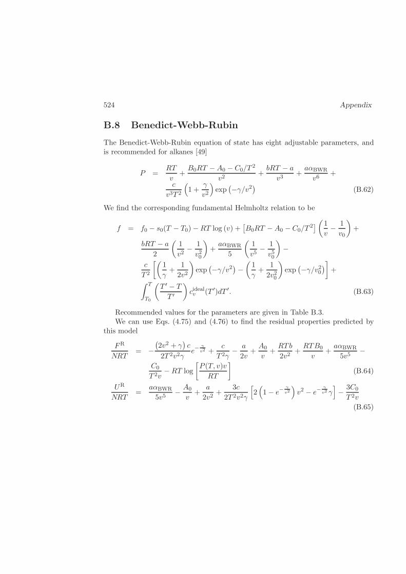
524 Appendix
B.8 Benedict-Webb-Rubin
The Benedict-Webb-Rubin equation of state has eight adjustable parameters, andis recommended for alkanes [49]
P =RT
v+B0RT −A0 − C0/T
2
v2+bRT − a
v3+aαBWR
v6+
c
v3T 2
(
1 +γ
v2
)
exp(−γ/v2
)(B.62)
We find the corresponding fundamental Helmholtz relation to be
f = f0 − s0(T − T0)−RT log (v) +[B0RT −A0 −C0/T
2](1
v− 1
v0
)
+
bRT − a
2
(1
v2− 1
v20
)
+aαBWR
5
(1
v5− 1
v50
)
−
c
T 2
[(1
γ+
1
2v2
)
exp(−γ/v2
)−(1
γ+
1
2v20
)
exp(−γ/v20
)]
+
∫ T
T0
(T ′ − T
T ′
)
cidealv (T ′)dT ′. (B.63)
Recommended values for the parameters are given in Table B.3.We can use Eqs. (4.75) and (4.76) to find the residual properties predicted by
this model
FR
NRT= −
(2v2 + γ
)c
2T 2v2γe−
γ
v2 +c
T 2γ− a
2v+A0
v+RTb
2v2+RTB0
v+aαBWR
5v5−
C0
T 2v−RT log
[P (T, v)v
RT
]
(B.64)
UR
NRT=
aαBWR
5v5− A0
v+
a
2v2+
3c
2T 2v2γ
[
2(
1− e−γ
v2
)
v2 − e−γ
v2 γ]
− 3C0
T 2v
(B.65)
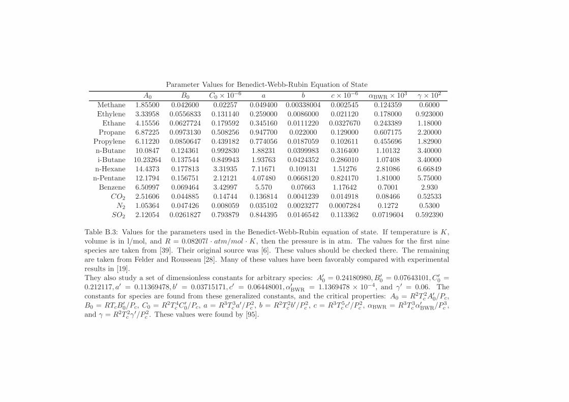
Parameter Values for Benedict-Webb-Rubin Equation of State
A0 B0 C0 × 10−6 a b c× 10−6 αBWR × 103 γ × 102
Methane 1.85500 0.042600 0.02257 0.049400 0.00338004 0.002545 0.124359 0.6000Ethylene 3.33958 0.0556833 0.131140 0.259000 0.0086000 0.021120 0.178000 0.923000Ethane 4.15556 0.0627724 0.179592 0.345160 0.0111220 0.0327670 0.243389 1.18000
Propane 6.87225 0.0973130 0.508256 0.947700 0.022000 0.129000 0.607175 2.20000Propylene 6.11220 0.0850647 0.439182 0.774056 0.0187059 0.102611 0.455696 1.82900n-Butane 10.0847 0.124361 0.992830 1.88231 0.0399983 0.316400 1.10132 3.40000i-Butane 10.23264 0.137544 0.849943 1.93763 0.0424352 0.286010 1.07408 3.40000n-Hexane 14.4373 0.177813 3.31935 7.11671 0.109131 1.51276 2.81086 6.66849n-Pentane 12.1794 0.156751 2.12121 4.07480 0.0668120 0.824170 1.81000 5.75000Benzene 6.50997 0.069464 3.42997 5.570 0.07663 1.17642 0.7001 2.930
CO2 2.51606 0.044885 0.14744 0.136814 0.0041239 0.014918 0.08466 0.52533N2 1.05364 0.047426 0.008059 0.035102 0.0023277 0.0007284 0.1272 0.5300SO2 2.12054 0.0261827 0.793879 0.844395 0.0146542 0.113362 0.0719604 0.592390
Table B.3: Values for the parameters used in the Benedict-Webb-Rubin equation of state. If temperature is K,volume is in l/mol, and R = 0.08207l · atm/mol · K, then the pressure is in atm. The values for the first ninespecies are taken from [39]. Their original source was [6]. These values should be checked there. The remainingare taken from Felder and Rousseau [28]. Many of these values have been favorably compared with experimentalresults in [19].They also study a set of dimensionless constants for arbitrary species: A′
0 = 0.24180980, B′0 = 0.07643101, C ′
0 =0.212117, a′ = 0.11369478, b′ = 0.03715171, c′ = 0.06448001, α′
BWR = 1.1369478 × 10⁻⁴, and γ′ = 0.06. Theconstants for species are found from these generalized constants, and the critical properties: A0 = R2T 2
c A′0/Pc,
B0 = RTcB′0/Pc, C0 = R2T 4
c C′0/Pc, a = R3T 3
c a′/P 2
c , b = R2T 2c b
′/P 2c , c = R3T 5
c c′/P 2
c , αBWR = R3T 3c α
′BWR/P
3c ,
and γ = R2T 2c γ
′/P 2c . These values were found by [95].
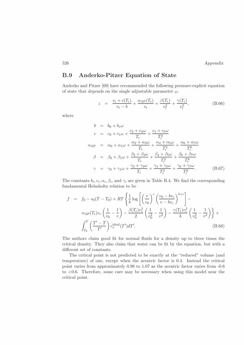
526 Appendix
B.9 Anderko-Pitzer Equation of State
Anderko and Pitzer [69] have recommended the following pressure-explicit equationof state that depends on the single adjustable parameter ω.
z =vr + c(Tr)
vr − b+αAP(Tr)
vr+β(Tr)
v2r+γ(Tr)
v3r, (B.66)
where
b = b0 + b1ω
c = c0 + c1ω +c2 + c3ω
Tr+c4 + c5ω
T 2r
αAP = α0 + α1ω +α2 + α3ω
Tr+α4 + α5ω
T 2r
+α6 + α7ω
T 6r
β = β0 + β1ω +β2 + β3ω
Tr+β4 + β5ω
T 2r
+β6 + β7ω
T 6r
γ = γ0 + γ1ω +γ2 + γ3ω
Tr+γ4 + γ5ω
T 2r
+γ6 + γ7ω
T 6r
. (B.67)
The constants bi, ci, αi, βi, and γi are given in Table B.4. We find the correspondingfundamental Helmholtz relation to be
f = f0 − s0(T − T0) +RT
1
blog
[(v
v0
)c(v0 − bvcv − bvc
)b+c]
−
αAP(Tr)vc
(1
v0− 1
v
)
− β(Tr)v2c
2
(1
v20− 1
v2
)
− γ(Tr)v3c
3
(1
v30− 1
v3
)
+
∫ T
T0
(T ′ − T
T ′
)
cidealv (T ′)dT ′. (B.68)
The authors claim good fit for normal fluids for a density up to three times thecritical density. They also claim that water can be fit by the equation, but with adifferent set of constants.
The critical point is not predicted to be exactly at the “reduced” volume (andtemperature) of one, except when the acentric factor is 0.4. Instead the criticalpoint varies from approximately 0.98 to 1.07 as the acentric factor varies from -0.6to +0.6. Therefore, some care may be necessary when using this model near thecritical point.
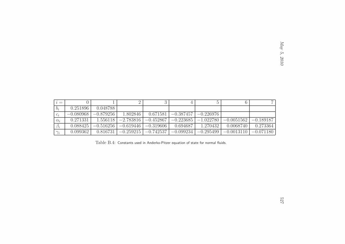
May5,2010
527
i = 0 1 2 3 4 5 6 7bi 0.251896 0.048788ci −0.080968 −0.879256 1.802846 0.671581 −0.387457 −0.226976αi 0.271331 1.556118 −2.783816 −0.452867 −0.223685 −1.022780 −0.0051562 −0.189187βi 0.088425 −0.516256 −0.619446 −0.319606 0.694687 1.270432 0.0068740 0.273364γi 0.099362 0.816731 −0.259215 −0.742537 −0.099234 −0.295499 −0.0013110 −0.071180
Table B.4: Constants used in Anderko-Pitzer equation of state for normal fluids.

528 Appendix
Appendix C
Microscopic Balances for OpenSystems
The starting point in the derivation of all microscopic balances is a differentialvolume element.1 In the simplest form, this element is a cube with edges of length∆x, ∆y and ∆z (See Figure C.1).
We assume that the fluid in this element is in an equilibrium state, determinedby the local instantaneous values of its thermodynamic quantities (e.g., temperatureand pressure). These quantities can vary with time and position. We call this thelocal equilibrium assumption.
Suppose that, from a thermodynamics point of view, we have temperature andpressure as ‘independent variables’. These quantities are now written as field vari-ables, meaning that they vary with time and position: T (~r, t), P (~r, t). We considera fluid that has mass density ρ(~r, t) = Mw(~r, t)/v(~r, t) (mass/volume), whereMw(~r, t) is the molecular weight of the fluid at position ~r and time t, which mayvary because of composition changes, and v(~r, t) is the specific volume under thosethermodynamic conditions.
Any quantity in this element (e.g., mass, momentum, or energy) must satisfythe balance relation:
Rate of
Accumulation
=
Flow
Rate In
−
FlowRate Out
+
Rate ofCreation
−
Rate ofDestruction
(C.1)
We first consider the mass balance in detail.
1Most derivations in this section are given in greater detail in [10]. This section may be skimmedby the student unfamiliar with the subject transport phenomena.
529
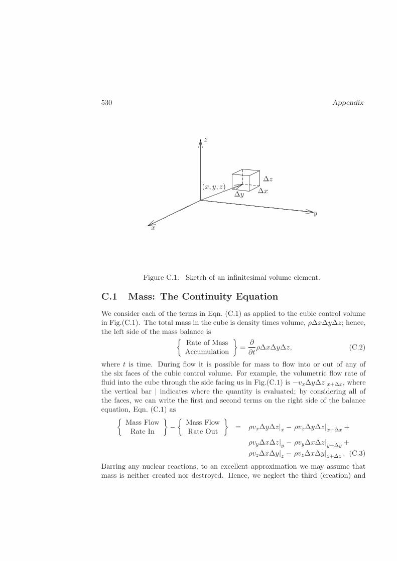
530 Appendix
z
y
x
∆z
∆y ∆x(x, y, z)
Figure C.1: Sketch of an infinitesimal volume element.
C.1 Mass: The Continuity Equation
We consider each of the terms in Eqn. (C.1) as applied to the cubic control volumein Fig.(C.1). The total mass in the cube is density times volume, ρ∆x∆y∆z; hence,the left side of the mass balance is
Rate of MassAccumulation
=∂
∂tρ∆x∆y∆z, (C.2)
where t is time. During flow it is possible for mass to flow into or out of any ofthe six faces of the cubic control volume. For example, the volumetric flow rate offluid into the cube through the side facing us in Fig.(C.1) is −vx∆y∆z|x+∆x, wherethe vertical bar | indicates where the quantity is evaluated; by considering all ofthe faces, we can write the first and second terms on the right side of the balanceequation, Eqn. (C.1) as
Mass FlowRate In
−
Mass FlowRate Out
= ρvx∆y∆z|x − ρvx∆y∆z|x+∆x +
ρvy∆x∆z|y − ρvy∆x∆z|y+∆y +
ρvz∆x∆y|z − ρvz∆x∆y|z+∆z . (C.3)
Barring any nuclear reactions, to an excellent approximation we may assume thatmass is neither created nor destroyed. Hence, we neglect the third (creation) and
May 5, 2010 531
fourth (destruction) terms on the right side of Eqn. (C.1). We put Eqn. (C.2) andEqn. (C.3) into the balance equation and divide by the volume of the cube ∆x∆y∆zto obtain
∂ρ
∂t= −
ρvx|x+∆x − ρvx|x∆x
−ρvy|y+∆y − ρvy|y
∆y−ρvz|z+∆z − ρvz|z
∆z. (C.4)
If we let the volume of the cube go to zero ∆x→ 0, ∆y → 0 ∆z → 0, then we canuse the definition of a derivative to write Eqn. (C.4) in differential form as
∂ρ
∂t= − ∂
∂xρvx −
∂
∂yρvy −
∂
∂zρvz = −∇ · (ρ~v) . (C.5)
Because it plays such an important role in transport phenomena, we have intro-duced the vector differential operator
∇ := ~δx∂
∂x+ ~δy
∂
∂y+ ~δz
∂
∂z, (C.6)
where ~δx is the unit vector that points in the x direction. We have also introducedthe fluid velocity vector ~v, which may be distinguished from the specific volume vwhich is light-faced, instead of bold-faced. We have also used the dot (or scalar)product “·”. We call Eqn. (C.5) the microscopic mass balance, or more com-monly the continuity equation.
We may also apply the balance relation Eqn. (C.1) to the moles of a single speciesk to obtain the continuity equation for species k2
∂ck∂t
+∇ · (ck~v) = −∇ · ~Jk −Rk, (C.7)
where ck is the molar concentration (moles/volume), ~Jk is the molar flux relativeto ~v (moles/area/volume/time), and Rk is the reaction rate (moles/volume/time),all of species k.
C.2 Momentum: The Equation of Motion
A similar balance can be performed on the momentum in the fluid.3 However, wemust now allow for the creation or destruction of momentum through forces at the
2See [10]: After eliminating ~nB from Eqn. (18.1–7) using Eqn. (V) of Table 16.1–3, multiply theequation by the molecular weight of species k to arrive at this form for the continuity equation.
3This and subsequent subsections use differential tensor calculus, which may be reviewed in theappendix of [10].
532 Appendix
face of the cube (through the extra stress tensor ~~τ and pressure P ), and throughbody forces, such as gravity. Such a derivation yields themicroscopic momentumbalance, sometimes called Cauchy’s equation4
∂
∂t(ρ~v) +∇ · (ρ~v~v) = −∇P + ρ~g +∇ · ~~τ , (C.8)
where we have introduced the gravity vector ~g, and the extra stress tensor ~~τ ,which describes the surface forces transmitted through the fluid per unit area ofcontact.
If we assume that the fluid is Newtonian (e.g., water) with viscosity ηs
~~τ = ηs
[
∇~v + (∇~v)†]
, Newtonian fluid (C.9)
and has constant material properties, then we may eliminate the stress tensor in theexpression to write
ρ∂
∂t~v + ρ~v · ∇~v = −∇P + ηs∇ · ∇~v + ρ~g, (C.10)
where ηs is the (constant) viscosity of the fluid. Eqn. (C.10) is called the Navier-Stokes equation. The superscript dagger in Eqn. (C.9) indicates taking the trans-pose. We may rewrite this equation using two additional definitions that are centralin transport phenomena; the substantial derivative is defined as
D
Dt:=
∂
∂t+ ~v · ∇, (C.11)
and may be thought of as finding the change in time of a quantity as one follows afluid element along a streamline. The Laplacian is defined as ∇2 := ∇ · ∇, whichmay be used to rewrite Eqn. (C.10)
ρD
Dt~v = −∇P + ηs∇2~v + ρ~g. (C.12)
This equation is central in momentum transport, or fluid dynamics [10, Eqn. (3.2-20)]; [8, Eqn. (B)].
If we take the dot product of each term in Eqn. (C.8) with the vector ~v, it ispossible to derive themicroscopic mechanical energy balance [10, Eqn. (3.3-2)].
∂
∂t
(1
2ρ|~v|2
)
+∇ ·(1
2ρ|~v|2~v
)
= −∇ · ρ~v + P (∇ · ~v)
+∇ · ~~τ · ~v − ~~τ : ∇~v + ρ~v · ~g. (C.13)
4Note, however, that we use the opposite sign convention for the stress tensor as that in [10,Eqn. (3.2-10)]
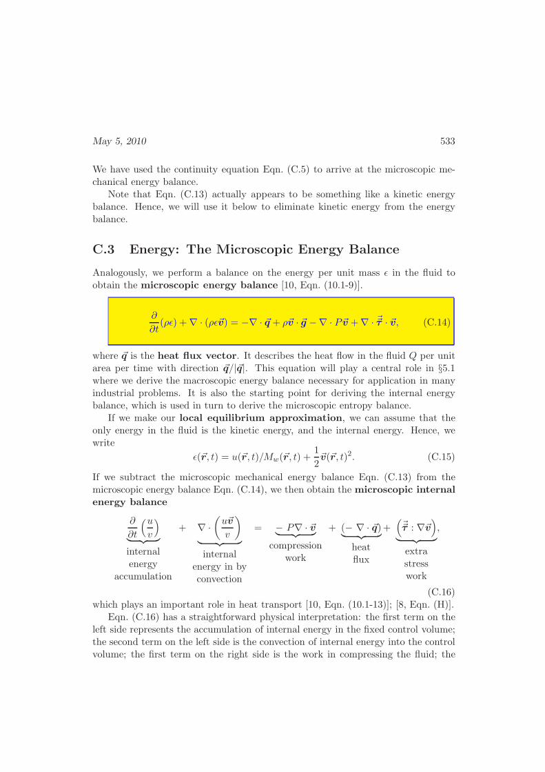
May 5, 2010 533
We have used the continuity equation Eqn. (C.5) to arrive at the microscopic me-chanical energy balance.
Note that Eqn. (C.13) actually appears to be something like a kinetic energybalance. Hence, we will use it below to eliminate kinetic energy from the energybalance.
C.3 Energy: The Microscopic Energy Balance
Analogously, we perform a balance on the energy per unit mass ǫ in the fluid toobtain the microscopic energy balance [10, Eqn. (10.1-9)].
∂
∂t(ρǫ) +∇ · (ρǫ~v) = −∇ · ~q + ρ~v · ~g −∇ · P~v +∇ · ~~τ · ~v, (C.14)
where ~q is the heat flux vector. It describes the heat flow in the fluid Q per unitarea per time with direction ~q/|~q|. This equation will play a central role in §5.1where we derive the macroscopic energy balance necessary for application in manyindustrial problems. It is also the starting point for deriving the internal energybalance, which is used in turn to derive the microscopic entropy balance.
If we make our local equilibrium approximation, we can assume that theonly energy in the fluid is the kinetic energy, and the internal energy. Hence, wewrite
ǫ(~r, t) = u(~r, t)/Mw(~r, t) +1
2~v(~r, t)2. (C.15)
If we subtract the microscopic mechanical energy balance Eqn. (C.13) from themicroscopic energy balance Eqn. (C.14), we then obtain the microscopic internalenergy balance
∂
∂t
(u
v
)
︸ ︷︷ ︸
internalenergy
accumulation
+ ∇ ·(u~v
v
)
︸ ︷︷ ︸
internalenergy in byconvection
= − P∇ · ~v︸ ︷︷ ︸
compressionwork
+ (− ∇ · ~q)︸ ︷︷ ︸
heatflux
+(~~τ : ∇~v
)
︸ ︷︷ ︸
extrastresswork
,
(C.16)which plays an important role in heat transport [10, Eqn. (10.1-13)]; [8, Eqn. (H)].
Eqn. (C.16) has a straightforward physical interpretation: the first term on theleft side represents the accumulation of internal energy in the fixed control volume;the second term on the left side is the convection of internal energy into the controlvolume; the first term on the right side is the work in compressing the fluid; the
534 Appendix
second term on the right side is the heat flow into the volume, and the last term iswork done by the surrounding fluid to deform the control volume.
We mention in passing that in transport phenomena this equation is typicallyused to calculate temperature fields. One does this by writing a differential forinternal energy in (T, v) and using the local equilibrium assumption to arrive at anevolution equation for temperature [10, p.315].
C.4 Entropy: The Microscopic Entropy Balance
We use the microscopic internal energy balance to derive the microscopic entropybalance. The derivation of this equation is far less common than the above equations.Hence, we show in more detail its derivation in a simplified system.5
We make the following assumptions for our simplified system:
• The fluid is composed of only one component.
• The fluid is Newtonian and incompressible, so that its extra stress tensor isdescribed by Eqn. (C.9).
Under these assumptions, we can rewrite Eqn. (C.16)
ρD
Dt
(u
Mw
)
+ P∇ · ~v = −∇ · ~q + ηsΦv, pure, Newtonian fluid, (C.17)
where
Φv :=1
2
[
∇~v + (∇~v)†]
:[
∇~v + (∇~v)†]
, (C.18)
is called the dissipation function. We have also used the continuity equationto rewrite the left side of the equation. We can further simplify this equation bymaking use of the continuity equation (C.5) in the form
∇ · ~v = −1
ρ
Dρ
Dt= − v
Mw
D
Dt
(Mw
v
)
. (C.19)
For a pure-component system, the molecular weight is constant, and may be pulledoutside the substantial derivative. Thus, Eqn. (C.17) can be written
1
v
[Du
Dt+ P
Dv
Dt
]
= −∇ · ~q + ηsΦv, pure, Newtonian fluid (C.20)
5The derivation here closely follows that of [26].
May 5, 2010 535
which is the starting point for our derivation of the simplified microscopic entropybalance. The left side of this equation can be simplified using the differential forinternal energy Eqn. (2.27) and the chain rule Eqn. (A.8) to write
Du
Dt+ P
Dv
Dt= T
Ds
Dt, (C.21)
We insert Eqn. (C.21) into Eqn. (C.20), and divide by T to obtain the simplifiedmicroscopic entropy balance
1
v
Ds
Dt︸ ︷︷ ︸
entropyaccumulation
= +
(
− ∇ · ~qT
)
︸ ︷︷ ︸
net fluxof entropy
+ ~q · ∇(1
T
)
+ηsTΦv
︸ ︷︷ ︸
entropygeneration
(C.22)
valid for a pure-component, Newtonian fluid. The equation has straightforwardphysical interpretation: the left side describes the accumulation of entropy in a fluidelement convected along a streamline; the first term on the right side describes theflux of entropy into the element from heat, the second and third terms yield thecreation of entropy per unit volume inside the volume element from temperaturegradients and viscous dissipation, respectively.
Example C.4.1 Calculate the entropy generation per unit volume for a Newtonianfluid of constant material properties in steady laminar flow in a pipe of constantwall temperature.
Solution: The velocity field and temperature field for the geometry of thisproblem are already known. The steady, laminar velocity field for a Newto-nian fluid with constant viscosity and density is parabolic in the z direction ofcylindrical coordinates6
vz = vmax
[
1−( r
R
)2]
, (C.23)
where R is the pipe radius, r is the radial coordinate, and vmax is the maximumvelocity, known for given pressure drop, pipe length and fluid viscosity. Thisrelation is obtained by solving Eqn. (C.12) for the prescribed geometry, whileassuming steady state and neglecting end effects.
The temperature in the fluid is not uniform because of viscous dissipation.By solving Eqn. (C.16) for a fluid with constant viscosity, density and thermalconductivity, the temperature field may be found [9, pp.218–220]
T (r) = Tw +ηsv
2max
4k
[
1−( r
R
)4]
, (C.24)
6The solution may be found, for example in [10], Eqn. (2.3–16)
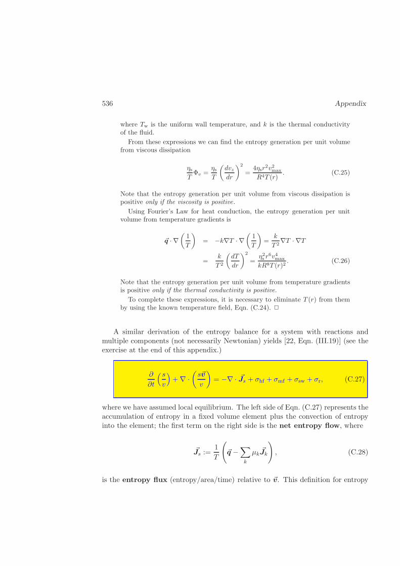
536 Appendix
where Tw is the uniform wall temperature, and k is the thermal conductivityof the fluid.
From these expressions we can find the entropy generation per unit volumefrom viscous dissipation
ηsTΦv =
ηsT
(dvzdr
)2
=4ηsr
2v2max
R4T (r). (C.25)
Note that the entropy generation per unit volume from viscous dissipation ispositive only if the viscosity is positive.
Using Fourier’s Law for heat conduction, the entropy generation per unitvolume from temperature gradients is
~q · ∇(1
T
)
= −k∇T · ∇(1
T
)
=k
T 2∇T · ∇T
=k
T 2
(dT
dr
)2
=η2s r
6v4max
kR8T (r)2. (C.26)
Note that the entropy generation per unit volume from temperature gradientsis positive only if the thermal conductivity is positive.
To complete these expressions, it is necessary to eliminate T (r) from themby using the known temperature field, Eqn. (C.24). 2
A similar derivation of the entropy balance for a system with reactions andmultiple components (not necessarily Newtonian) yields [22, Eqn. (III.19)] (see theexercise at the end of this appendix.)
∂
∂t
(s
v
)
+∇ ·(s~v
v
)
= −∇ · ~Js + σhf + σmf + σsw + σr, (C.27)
where we have assumed local equilibrium. The left side of Eqn. (C.27) represents theaccumulation of entropy in a fixed volume element plus the convection of entropyinto the element; the first term on the right side is the net entropy flow, where
~Js :=1
T
(
~q −∑
k
µk ~Jk
)
, (C.28)
is the entropy flux (entropy/area/time) relative to ~v. This definition for entropy
May 5, 2010 537
flux is reminiscent of the differential for S, Eqn. (2.29)
dS =1
TdU +
P
TdV −
∑
k
µkTdNk
=1
T( dQ+ dW ) +
P
TdV −
∑
k
µkTdNk
=1
T
(
dQrev −∑
k
µkdNk
)
. (C.29)
We have used energy conservation Eqn. (2.1) to obtain the second line, and assumedonly reversible work to obtain the third line—consistent with our local equilibriumassumption. Compare the last two equations.
The new terms on the right side of Eqn. (C.27) represent the creation of entropyfrom, respectively, heat fluxes, molar fluxes, stress work, and reactions
Tσhf := − ~Js · ∇T (C.30)
Tσmf := −m∑
k=1
~Jk · ∇µk (C.31)
Tσsw := −~~τ : ∇~v (C.32)
Tσr := −m∑
k=1
Rkµk. (C.33)
Eqn. (C.27) is the final goal of this subsection. It plays a central role in irreversiblethermodynamics [54, §2.3]; [22]; [53, §15.5]. A fundamental tenet of irreversiblethermodynamics is that the generation terms given by Eqs. (C.30) through (C.33),should be non-negative in order to satisfy the second law of thermodynamics, Pos-tulate IV. Hence, if we assume that heat flux is described by Fourier’s Law of heatconduction, then the thermal conductivity must be positive. Similarly, a Newtonianfluid must have positive viscosity in order to be consistent with the principles ofirreversible thermodynamics.
Eqs. (C.5), (C.14) and (C.27) are used to derive the macroscopic balanceequations, given in §5.1.
C.5 Entropy Flux and Generation in Laminar Flow
In industrial application, an engineer does not typically know entropy generationor entropy flux accurately. However, the following example shows how detailedinformation about the flow process can be used to estimate these quantities.
538 Appendix
Example C.5.1 Using results from transport phenomena and §C, calculate the to-tal entropy generation and entropy flux for a Newtonian fluid of constant materialproperties in steady laminar flow in a pipe of constant wall temperature and lengthL.
Solution: The entropy generation per unit volume σsw is found in ExampleC.4.1. We may integrate these results over the volume of the pipe to find thetotal entropy generation. The entropy generation from stress work is just thecontribution from Newtonian viscous dissipation
Σsw =
∫ L
0
∫ 2π
0
∫ R
0
ηsTΦvrdrdθdz
= 2πL
∫ R
0
4ηsr3v2max
R4T (r)dr
= 8πLk log
(
1 +ηsv
2max
4kTw
)
. (C.34)
We used Eqn. (C.25) to obtain the second line, and Eqn. (C.24) to obtain thethird. Similarly, we may find the entropy generation from heat flows
Σhf =
∫ L
0
∫ 2π
0
∫ R
0
~q · ∇(1
T
)
rdrdθdz
= 2πL
∫ R
0
k
T (r)2
(dT
dr
)2
dr
= 2πL
∫ R
0
η2s r7v4max
kR8T (r)2dr
= 8πLk
[ηsv
2max
4kTw− log
(
1 +ηsv
2max
4kTw
)]
(C.35)
Note that we used Fourier’s Law to obtain the second line, Eqn. (C.26) toobtain the third line, and Eqn. (C.24) to obtain the fourth.
Finally, we may obtain the entropy flux out of the walls of the pipe, sincethere is no molar flux at the walls
∫∫
A
~n · k∇TdAT
= −∫ L
0
∫ 2π
0
qr(R)
T (R)Rdθdz
=2πRLk
Tw
dT
dr
∣∣∣∣r=R
= −2πLηsv2max
Tw. (C.36)
To obtain the second line, we performed the integration, and used Fourier’sLaw. We used the known temperature field Eqn. (C.24) to obtain the third.
May 5, 2010 539
If we combine the results in Eqs. (C.34), (C.35) and (C.36), we find that
∫∫
A
~n · k∇TdAT
+ Σsw + Σhf = 0. (C.37)
Hence, the macroscopic entropy balance Eqn. (5.7) states that the inlet andexit specific entropies of the laminar pipe flow with isothermal walls are thesame
sout = sin, (C.38)
since mass balance requires that the mass flows are the same in and out: mout =min.
Actually, we can derive this result more simply by integrating along a fluidstreamline in the pipe. The streamlines in laminar flow are lines of constant rand θ. As the fluid element changes its z coordinate, the pressure changes butthe temperature remains constant. Hence, the change in entropy for the fluidelement from inlet to exit can be found as
sout − sin =
∫ Pout
Pin
(∂s
∂P
)
T
dP
= −∫ Pout
Pin
(∂v
∂T
)
P
dP
= 0. (C.39)
The second line follows from the Maxwell relation (§3.3), and the third linefollows because the fluid is assumed incompressible, and, hence, the specificvolume v is a constant.
Therefore, we find that all of the entropy generated in the pipe is conductedout the walls, and the fluid entropy stays constant along each streamline. 2
Unlike the fluid in this example, a real fluid is compressible, of course. It is inter-esting to estimate the sign sout − sin, however. Above, we found for a compressiblefluid that
sout − sin = −∫ Pout
Pin
v(T, P )α(T, P )dP, (C.40)
where α is the coefficient of thermal expansion defined by Eqn. (3.60). Most realfluids exhibit positive values for α. Since, Pin > Pout, we find that most real fluidswould yield sout > sin. However, some fluids such as water near the freezing pointexhibit a negative value for α; hence, these would show that entropy decreases alongthe pipe.
Exercise: Derive the microscopic entropy balance Eqn. (C.27) in the following way:
540 Appendix
a. Using equilibrium thermodynamic manipulations, show that
d( s
v
)
= d
(S
V
)
=1
T
[
d(u
v
)
−∑
i
µidci
]
(Hint: You may need to use the Euler relation.)b. Using the chain rule, show that this expression, within the local equilibrium
approximation, leads to
D
Dt
(s
v
)
=1
T
[
D
Dt
(u
v
)
−∑
i
µiDciDt
]
c. Show that for any function ψ
∂ψ
∂t+∇ · (ψ~v) = Dψ
Dt+ ψ∇ · ~v
d. Now combine the results from parts b. and c. (starting with ψ = s/v), alongwith the internal energy balance Eqn. (C.16) and the continuity equation for speciesk, Eqn. (C.7) to derive the microscopic entropy balance, Eqn. (C.27).
Appendix D
Physical Properties andReferences
D.1 Websites with data and programs
There are many sources available for finding physical properties, such as criticalproperties, heat capacities, molecular weights, etc. Besides texts, many computerpackages may be accessed for the data. Below is a list of URLs that may be used tofind data for many species and computer programs on the web. Most of these arefree, but may contain links to services requiring fees. Since we have no control overtheir content, we cannot be responsible for the accuracy or usefulness of the infor-mation supplied. URLs are not particularly stable, but they should be obtainablefrom a search engine, such as Google.
• The National Institute for Standards and Technology keeps a tremendousamount of data online, and contains links to other sites. They also sell catalogsand computer software:
http://properties.nist.gov/
• Many thermodynamic, transport, and physical properties are stored by theAmerican Institute of Chemical Engineers at the Design Institute for PhysicalProperty Data. A large database has free access for students (http://dippr.byu.edu/).
• Free software, and data, such as molecular weight, critical pressure and criticaltemperature may be found for gases at Flexware (http://www.flexwareinc.com/).
• Prof. G.R. Mansoori of the University of Illinois-Chicago maintains a websitewith links to many other web pages that contain data, or computer programsfor thermodynamic calculation:
541
542 Appendix
http://www.uic.edu/˜mansoori/Thermodynamic.Data.and.Property html
• The University of Texas has a Javascript program called ‘ThermoDex’ thatsearches their bookshelves for thermodynamic data. The program returnsonly the reference for the book, however:
http://thermodex.lib.utexas.edu/
• The Center for Research in Computational Thermochemistry at Ecole Poly-technique de Montreal has a site that contains conversion factors, heat capac-ities, formation properties, links, calculators and much more at
http://www.crct.polymtl.ca/fact/websites.htm
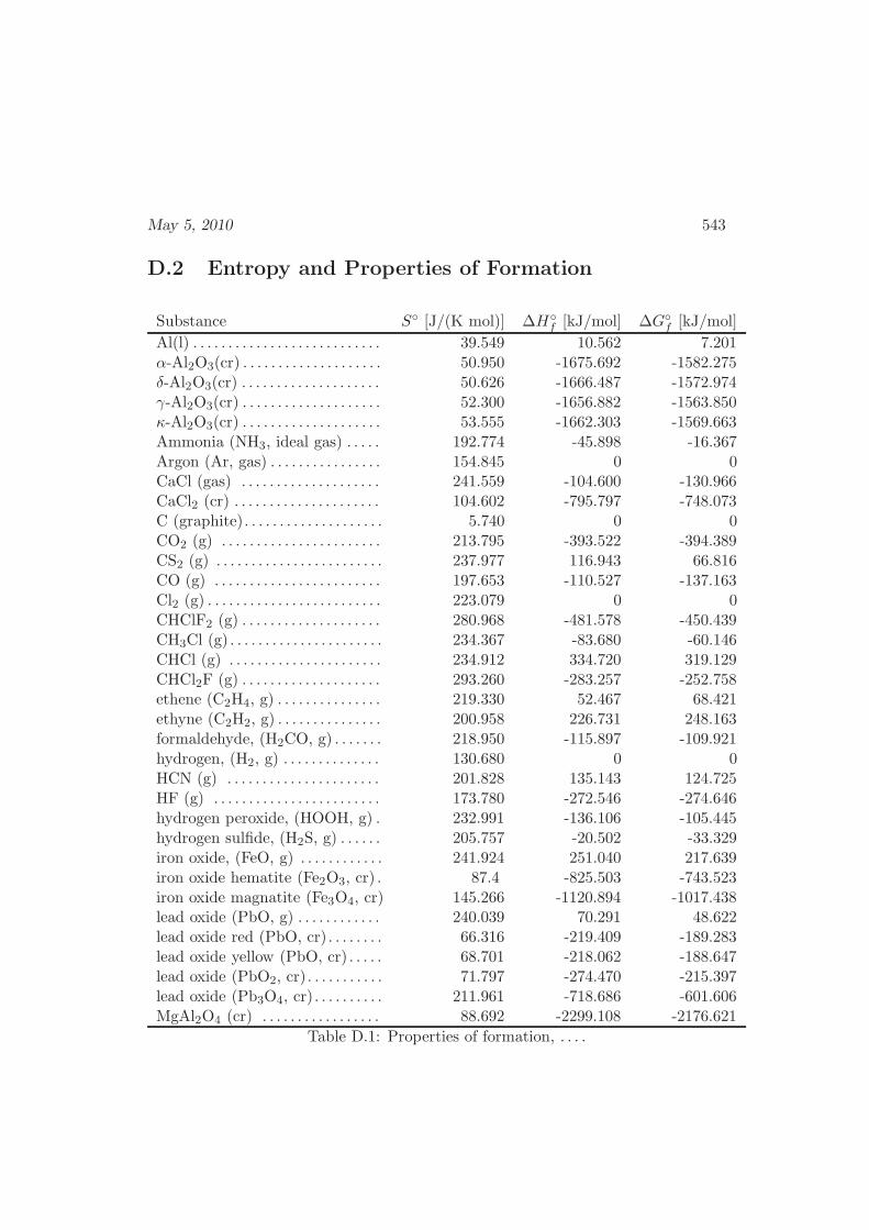
May 5, 2010 543
D.2 Entropy and Properties of Formation
Substance S [J/(K mol)] ∆Hf [kJ/mol] ∆G
f [kJ/mol]
Al(l) . . . . . . . . . . . . . . . . . . . . . . . . . . . 39.549 10.562 7.201α-Al2O3(cr) . . . . . . . . . . . . . . . . . . . . 50.950 -1675.692 -1582.275δ-Al2O3(cr) . . . . . . . . . . . . . . . . . . . . 50.626 -1666.487 -1572.974γ-Al2O3(cr) . . . . . . . . . . . . . . . . . . . . 52.300 -1656.882 -1563.850κ-Al2O3(cr) . . . . . . . . . . . . . . . . . . . . 53.555 -1662.303 -1569.663Ammonia (NH3, ideal gas) . . . . . 192.774 -45.898 -16.367Argon (Ar, gas) . . . . . . . . . . . . . . . . 154.845 0 0CaCl (gas) . . . . . . . . . . . . . . . . . . . . 241.559 -104.600 -130.966CaCl2 (cr) . . . . . . . . . . . . . . . . . . . . . 104.602 -795.797 -748.073C (graphite). . . . . . . . . . . . . . . . . . . . 5.740 0 0CO2 (g) . . . . . . . . . . . . . . . . . . . . . . . 213.795 -393.522 -394.389CS2 (g) . . . . . . . . . . . . . . . . . . . . . . . . 237.977 116.943 66.816CO (g) . . . . . . . . . . . . . . . . . . . . . . . . 197.653 -110.527 -137.163Cl2 (g) . . . . . . . . . . . . . . . . . . . . . . . . . 223.079 0 0CHClF2 (g) . . . . . . . . . . . . . . . . . . . . 280.968 -481.578 -450.439CH3Cl (g) . . . . . . . . . . . . . . . . . . . . . . 234.367 -83.680 -60.146CHCl (g) . . . . . . . . . . . . . . . . . . . . . . 234.912 334.720 319.129CHCl2F (g) . . . . . . . . . . . . . . . . . . . . 293.260 -283.257 -252.758ethene (C2H4, g) . . . . . . . . . . . . . . . 219.330 52.467 68.421ethyne (C2H2, g) . . . . . . . . . . . . . . . 200.958 226.731 248.163formaldehyde, (H2CO, g) . . . . . . . 218.950 -115.897 -109.921hydrogen, (H2, g) . . . . . . . . . . . . . . 130.680 0 0HCN (g) . . . . . . . . . . . . . . . . . . . . . . 201.828 135.143 124.725HF (g) . . . . . . . . . . . . . . . . . . . . . . . . 173.780 -272.546 -274.646hydrogen peroxide, (HOOH, g) . 232.991 -136.106 -105.445hydrogen sulfide, (H2S, g) . . . . . . 205.757 -20.502 -33.329iron oxide, (FeO, g) . . . . . . . . . . . . 241.924 251.040 217.639iron oxide hematite (Fe2O3, cr) . 87.4 -825.503 -743.523iron oxide magnatite (Fe3O4, cr) 145.266 -1120.894 -1017.438lead oxide (PbO, g) . . . . . . . . . . . . 240.039 70.291 48.622lead oxide red (PbO, cr) . . . . . . . . 66.316 -219.409 -189.283lead oxide yellow (PbO, cr) . . . . . 68.701 -218.062 -188.647lead oxide (PbO2, cr). . . . . . . . . . . 71.797 -274.470 -215.397lead oxide (Pb3O4, cr). . . . . . . . . . 211.961 -718.686 -601.606MgAl2O4 (cr) . . . . . . . . . . . . . . . . . 88.692 -2299.108 -2176.621
Table D.1: Properties of formation, . . . .
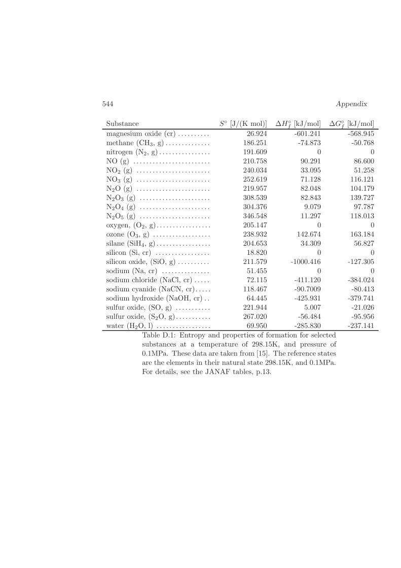
544 Appendix
Substance S [J/(K mol)] ∆Hf [kJ/mol] ∆G
f [kJ/mol]
magnesium oxide (cr) . . . . . . . . . . 26.924 -601.241 -568.945methane (CH3, g) . . . . . . . . . . . . . . 186.251 -74.873 -50.768nitrogen (N2, g) . . . . . . . . . . . . . . . . 191.609 0 0NO (g) . . . . . . . . . . . . . . . . . . . . . . . . 210.758 90.291 86.600NO2 (g) . . . . . . . . . . . . . . . . . . . . . . . 240.034 33.095 51.258NO3 (g) . . . . . . . . . . . . . . . . . . . . . . . 252.619 71.128 116.121N2O (g) . . . . . . . . . . . . . . . . . . . . . . . 219.957 82.048 104.179N2O3 (g) . . . . . . . . . . . . . . . . . . . . . . 308.539 82.843 139.727N2O4 (g) . . . . . . . . . . . . . . . . . . . . . . 304.376 9.079 97.787N2O5 (g) . . . . . . . . . . . . . . . . . . . . . . 346.548 11.297 118.013oxygen, (O2, g) . . . . . . . . . . . . . . . . . 205.147 0 0ozone (O3, g) . . . . . . . . . . . . . . . . . . 238.932 142.674 163.184silane (SiH4, g) . . . . . . . . . . . . . . . . . 204.653 34.309 56.827silicon (Si, cr) . . . . . . . . . . . . . . . . . 18.820 0 0silicon oxide, (SiO, g) . . . . . . . . . . 211.579 -1000.416 -127.305sodium (Na, cr) . . . . . . . . . . . . . . . 51.455 0 0sodium chloride (NaCl, cr) . . . . . 72.115 -411.120 -384.024sodium cyanide (NaCN, cr). . . . . 118.467 -90.7009 -80.413sodium hydroxide (NaOH, cr) . . 64.445 -425.931 -379.741sulfur oxide, (SO, g) . . . . . . . . . . . 221.944 5.007 -21.026sulfur oxide, (S2O, g) . . . . . . . . . . . 267.020 -56.484 -95.956water (H2O, l) . . . . . . . . . . . . . . . . . 69.950 -285.830 -237.141
Table D.1: Entropy and properties of formation for selectedsubstances at a temperature of 298.15K, and pressure of0.1MPa. These data are taken from [15]. The reference statesare the elements in their natural state 298.15K, and 0.1MPa.For details, see the JANAF tables, p.13.
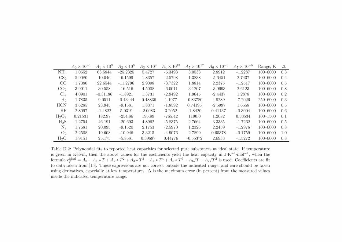
A0 × 10−1 A1 × 103 A2 × 106 A3 × 109 A4 × 1013 A5 × 1017 A6 × 10−3 A7 × 10−5 Range, K ∆
NH3 1.0552 63.5844 -25.2325 5.4727 -6.3493 3.0533 2.8912 -1.2287 100–6000 0.3CS2 5.9080 10.046 -6.1599 1.8357 -2.5798 1.3838 -5.6451 2.7437 100–6000 0.4CO 1.7080 22.6544 -11.2796 2.9098 -3.7322 1.8814 2.2375 -1.2517 100–6000 0.5CO2 3.9911 30.558 -16.516 4.5008 -6.0011 3.1207 -3.9693 2.6123 100–6000 0.8Cl2 4.0901 -0.31186 -1.8921 1.3731 -2.9492 1.9645 -2.4437 1.2878 100–6000 0.2H2 1.7835 9.0511 -0.43444 -0.48836 1.1977 -0.83780 4.9289 -7.2026 250–6000 0.3
HCN 3.6285 23.945 -9.1581 1.8371 -1.8592 0.74195 -2.5997 1.6558 100–6000 0.5HF 2.8097 -1.4822 5.0319 -2.0083 3.2052 -1.8420 0.41137 -0.3004 100–6000 0.6
H2O2 0.21531 182.97 -254.86 195.99 -765.42 1190.0 1.2082 0.33534 100–1500 0.1H2S 1.2754 46.191 -20.693 4.8962 -5.8375 2.7664 3.3335 -1.7262 100–6000 0.5N2 1.7681 20.095 -9.1520 2.1753 -2.5970 1.2326 2.2459 -1.2976 100–6000 0.8O2 2.2508 19.608 -10.946 3.3215 -4.9076 2.7899 0.65378 -0.1759 100–6000 1.0
H2O 1.9151 25.175 -5.8581 0.39697 0.44776 -0.55372 2.6933 -1.5272 100–6000 0.8
Table D.2: Polynomial fits to reported heat capacities for selected pure substances at ideal state. If temperatureis given in Kelvin, then the above values for the coefficients yield the heat capacity in J·K−1·mol−1, when theformula cidealP = A0 +A1 ∗ T +A2 ∗ T 2 +A3 ∗ T 3 +A4 ∗ T 4 +A5 ∗ T 5 +A6/T +A7/T
2 is used. Coefficients are fitto data taken from [15]. These expressions are not correct outside the indicated range, and care should be takenusing derivatives, especially at low temperatures. ∆ is the maximum error (in percent) from the measured valuesinside the indicated temperature range.
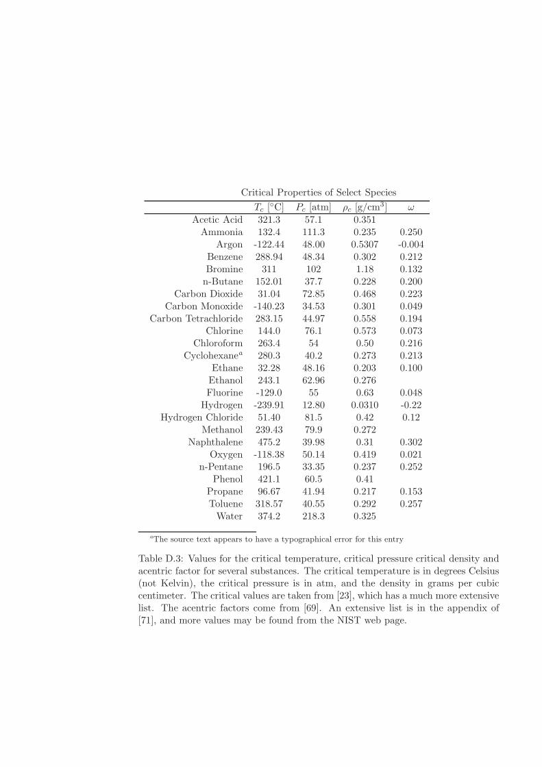
Critical Properties of Select Species
Tc [C] Pc [atm] ρc [g/cm
3] ω
Acetic Acid 321.3 57.1 0.351Ammonia 132.4 111.3 0.235 0.250
Argon -122.44 48.00 0.5307 -0.004Benzene 288.94 48.34 0.302 0.212Bromine 311 102 1.18 0.132n-Butane 152.01 37.7 0.228 0.200
Carbon Dioxide 31.04 72.85 0.468 0.223Carbon Monoxide -140.23 34.53 0.301 0.049
Carbon Tetrachloride 283.15 44.97 0.558 0.194Chlorine 144.0 76.1 0.573 0.073
Chloroform 263.4 54 0.50 0.216Cyclohexanea 280.3 40.2 0.273 0.213
Ethane 32.28 48.16 0.203 0.100Ethanol 243.1 62.96 0.276Fluorine -129.0 55 0.63 0.048
Hydrogen -239.91 12.80 0.0310 -0.22Hydrogen Chloride 51.40 81.5 0.42 0.12
Methanol 239.43 79.9 0.272Naphthalene 475.2 39.98 0.31 0.302
Oxygen -118.38 50.14 0.419 0.021n-Pentane 196.5 33.35 0.237 0.252
Phenol 421.1 60.5 0.41Propane 96.67 41.94 0.217 0.153Toluene 318.57 40.55 0.292 0.257Water 374.2 218.3 0.325
aThe source text appears to have a typographical error for this entry
Table D.3: Values for the critical temperature, critical pressure critical density andacentric factor for several substances. The critical temperature is in degrees Celsius(not Kelvin), the critical pressure is in atm, and the density in grams per cubiccentimeter. The critical values are taken from [23], which has a much more extensivelist. The acentric factors come from [69]. An extensive list is in the appendix of[71], and more values may be found from the NIST web page.
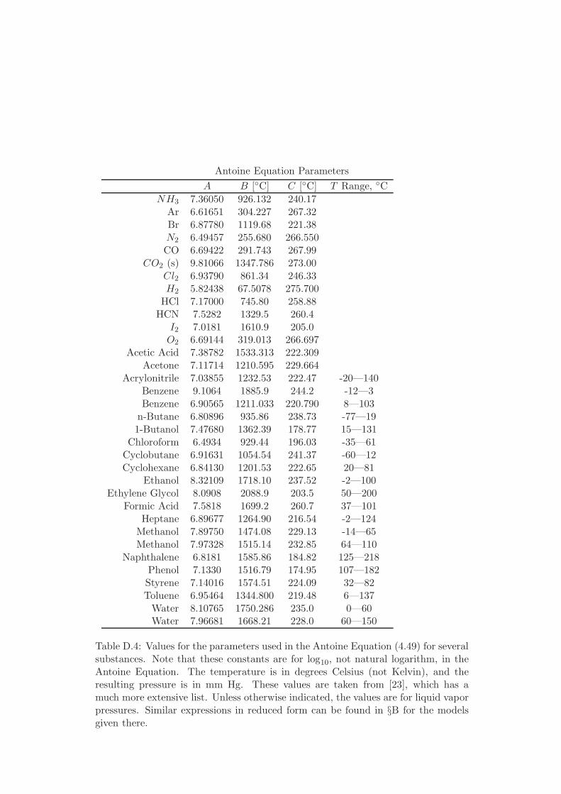
Antoine Equation Parameters
A B [C] C [C] T Range, CNH3 7.36050 926.132 240.17
Ar 6.61651 304.227 267.32Br 6.87780 1119.68 221.38N2 6.49457 255.680 266.550CO 6.69422 291.743 267.99
CO2 (s) 9.81066 1347.786 273.00Cl2 6.93790 861.34 246.33H2 5.82438 67.5078 275.700HCl 7.17000 745.80 258.88HCN 7.5282 1329.5 260.4
I2 7.0181 1610.9 205.0O2 6.69144 319.013 266.697
Acetic Acid 7.38782 1533.313 222.309Acetone 7.11714 1210.595 229.664
Acrylonitrile 7.03855 1232.53 222.47 -20—140Benzene 9.1064 1885.9 244.2 -12—3Benzene 6.90565 1211.033 220.790 8—103n-Butane 6.80896 935.86 238.73 -77—191-Butanol 7.47680 1362.39 178.77 15—131
Chloroform 6.4934 929.44 196.03 -35—61Cyclobutane 6.91631 1054.54 241.37 -60—12Cyclohexane 6.84130 1201.53 222.65 20—81
Ethanol 8.32109 1718.10 237.52 -2—100Ethylene Glycol 8.0908 2088.9 203.5 50—200
Formic Acid 7.5818 1699.2 260.7 37—101Heptane 6.89677 1264.90 216.54 -2—124
Methanol 7.89750 1474.08 229.13 -14—65Methanol 7.97328 1515.14 232.85 64—110
Naphthalene 6.8181 1585.86 184.82 125—218Phenol 7.1330 1516.79 174.95 107—182Styrene 7.14016 1574.51 224.09 32—82Toluene 6.95464 1344.800 219.48 6—137Water 8.10765 1750.286 235.0 0—60Water 7.96681 1668.21 228.0 60—150
Table D.4: Values for the parameters used in the Antoine Equation (4.49) for severalsubstances. Note that these constants are for log10, not natural logarithm, in theAntoine Equation. The temperature is in degrees Celsius (not Kelvin), and theresulting pressure is in mm Hg. These values are taken from [23], which has amuch more extensive list. Unless otherwise indicated, the values are for liquid vaporpressures. Similar expressions in reduced form can be found in §B for the modelsgiven there.

548 Appendix
D.3 Physical Constants
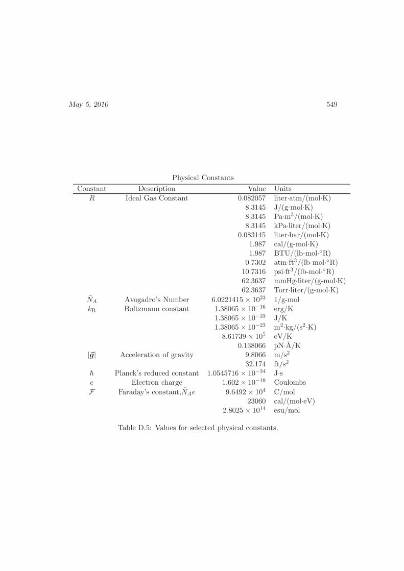
May 5, 2010 549
Physical Constants
Constant Description Value Units
R Ideal Gas Constant 0.082057 liter·atm/(mol·K)8.3145 J/(g-mol·K)8.3145 Pa·m3/(mol·K)8.3145 kPa·liter/(mol·K)
0.083145 liter·bar/(mol·K)1.987 cal/(g-mol·K)1.987 BTU/(lb-mol·R)0.7302 atm·ft3/(lb-mol·R)10.7316 psi·ft3/(lb-mol·R)62.3637 mmHg·liter/(g-mol·K)62.3637 Torr·liter/(g-mol·K)
NA Avogadro’s Number 6.0221415 × 10²³ 1/g-molkB Boltzmann constant 1.38065 × 10⁻¹⁶ erg/K
1.38065 × 10⁻²³ J/K1.38065 × 10−23 m2·kg/(s2·K)8.61739 × 105 eV/K
0.138066 pN·A/K|~g| Acceleration of gravity 9.8066 m/s2
32.174 ft/s2
h Planck’s reduced constant 1.0545716 × 10⁻³⁴ J·se Electron charge 1.602 × 10⁻¹⁹ Coulombs
F Faraday’s constant,NAe 9.6492 × 10⁴ C/mol23060 cal/(mol·eV)
2.8025 × 10¹⁴ esu/mol
Table D.5: Values for selected physical constants.
550 Appendix
D.4 Steam Tables
The following pages contain properties of steam in both English and SI units. Thesevalues were calculated using the 1967 IFC Formulations for Industrial Use, and notthe more accurate IAPWS-95 Formulation for General and Scientific Use.
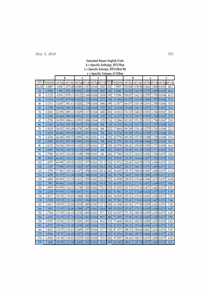
May 5, 2010 551
T(F) Psat(psia) sat liq sat vap sat liqsat vapsat liq sat vapT(F)Psat(psia) sat liq sat vap sat liqsat vapsat liq sat vap
32.018 0.0887 0.000 1075.48 0.0000 2.187 0.0160 3302 182 7.8505 150.006 1138.98 0.2662 1.808 0.0165 48.234 0.0960 1.996 1076.35 0.0041 2.180 0.0160 3062 186 8.5680 154.020 1140.55 0.2725 1.800 0.0165 44.438 0.1125 6.018 1078.11 0.0122 2.166 0.0160 2634 190 9.3396 158.037 1142.11 0.2787 1.793 0.0166 41.042 0.1314 10.035 1079.86 0.0202 2.153 0.0160 2272 194 10.1684 162.055 1143.65 0.2848 1.787 0.0166 37.846 0.1531 14.047 1081.61 0.0282 2.139 0.0160 1966 198 11.0577 166.075 1145.19 0.2910 1.780 0.0166 35.050 0.1780 18.054 1083.36 0.0361 2.126 0.0160 1705 202 12.0108 170.098 1146.71 0.2971 1.773 0.0167 32.454 0.2063 22.058 1085.11 0.0439 2.113 0.0160 1482 206 13.0312 174.123 1148.23 0.3031 1.766 0.0167 30.058 0.2384 26.060 1086.86 0.0516 2.101 0.0160 1292 210 14.1225 178.151 1149.73 0.3091 1.760 0.0167 27.862 0.2749 30.059 1088.61 0.0593 2.088 0.0160 1129 214 15.2886 182.181 1151.22 0.3151 1.754 0.0167 25.866 0.3163 34.056 1090.35 0.0670 2.076 0.0160 989 218 16.5332 186.214 1152.70 0.3211 1.747 0.0168 24.070 0.3629 38.052 1092.09 0.0745 2.065 0.0160 868 222 17.8604 190.249 1154.16 0.3270 1.741 0.0168 22.374 0.4155 42.046 1093.83 0.0821 2.053 0.0161 764 226 19.2742 194.288 1155.61 0.3329 1.735 0.0168 20.878 0.4746 46.040 1095.57 0.0895 2.041 0.0161 674 230 20.7790 198.330 1157.05 0.3388 1.729 0.0168 19.482 0.5409 50.033 1097.30 0.0969 2.030 0.0161 596 234 22.3791 202.38 1158.48 0.3446 1.723 0.0169 18.186 0.6152 54.026 1099.03 0.1043 2.019 0.0161 527 238 24.0790 206.42 1159.89 0.3505 1.717 0.0169 16.990 0.6981 58.018 1100.76 0.1115 2.009 0.0161 468 242 25.8833 210.48 1161.29 0.3562 1.711 0.0169 15.894 0.7906 62.010 1102.49 0.1188 1.998 0.0161 416 246 27.7969 214.53 1162.67 0.3620 1.706 0.0170 14.898 0.8936 66.003 1104.21 0.1260 1.988 0.0161 370.9 250 29.8247 218.59 1164.04 0.3677 1.700 0.0170 13.8102 1.0079 69.995 1105.92 0.1331 1.977 0.0161 331.1 254 31.9715 222.65 1165.39 0.3734 1.694 0.0170 12.9106 1.1347 73.988 1107.63 0.1402 1.967 0.0162 296.2 258 34.2427 226.72 1166.72 0.3791 1.689 0.0171 12.1110 1.2750 77.981 1109.34 0.1472 1.958 0.0162 265.4 262 36.6435 230.79 1168.04 0.3847 1.684 0.0171 11.4114 1.4299 81.975 1111.04 0.1542 1.948 0.0162 238.2 266 39.1794 234.87 1169.35 0.3904 1.678 0.0171 10.70118 1.6009 85.969 1112.74 0.1611 1.939 0.0162 214.2 270 41.8558 238.95 1170.64 0.3960 1.673 0.0172 10.06122 1.7891 89.964 1114.43 0.1680 1.929 0.0162 193.0 274 44.6785 243.03 1171.91 0.4015 1.668 0.0172 9.46126 1.9959 93.959 1116.12 0.1749 1.920 0.0162 174.1 278 47.6533 247.13 1173.16 0.4071 1.662 0.0172 8.91130 2.2230 97.955 1117.80 0.1817 1.911 0.0162 157.3 282 50.7861 251.22 1174.40 0.4126 1.657 0.0173 8.39134 2.4717 101.95 1119.47 0.1884 1.902 0.0163 142.4 286 54.0830 255.32 1175.61 0.4181 1.652 0.0173 7.91138 2.7438 105.95 1121.14 0.1951 1.894 0.0163 129.1 290 57.5501 259.43 1176.81 0.4236 1.647 0.0174 7.46142 3.0411 109.95 1122.80 0.2018 1.885 0.0163 117.2 294 61.1940 263.54 1177.99 0.4290 1.642 0.0174 7.04146 3.3653 113.95 1124.46 0.2084 1.877 0.0163 106.6 298 65.0209 267.65 1179.15 0.4345 1.638 0.0174 6.65150 3.7184 117.95 1126.10 0.2150 1.869 0.0163 97.1 302 69.0375 271.78 1180.30 0.4399 1.633 0.0175 6.29154 4.1025 121.95 1127.74 0.2216 1.861 0.0164 88.5 306 73.2505 275.90 1181.42 0.4453 1.628 0.0175 5.95158 4.5197 125.96 1129.37 0.2281 1.853 0.0164 80.8 310 77.6668 280.04 1182.52 0.4506 1.623 0.0176 5.63162 4.9722 129.96 1131.00 0.2345 1.845 0.0164 73.9 314 82.2933 284.18 1183.60 0.4560 1.619 0.0176 5.33166 5.4623 133.97 1132.61 0.2409 1.837 0.0164 67.7 318 87.1371 288.33 1184.66 0.4613 1.614 0.0176 5.05170 5.9926 137.97 1134.22 0.2473 1.830 0.0165 62.1 322 92.2054 292.48 1185.70 0.4666 1.609 0.0177 4.78174 6.5656 141.98 1135.81 0.2537 1.822 0.0165 57.0 326 97.5057 296.64 1186.71 0.4719 1.605 0.0177 4.54178 7.1840 145.99 1137.40 0.2600 1.815 0.0165 52.4 330 103.0453 300.81 1187.70 0.4772 1.600 0.0178 4.31
h s v
v = Specific Volume, ft^3/lbm
Saturated Steam: English Units
h = Specific Enthalpy, BTU/lbm
s = Specific Entropy, BTU/(lbm*R)
vh s
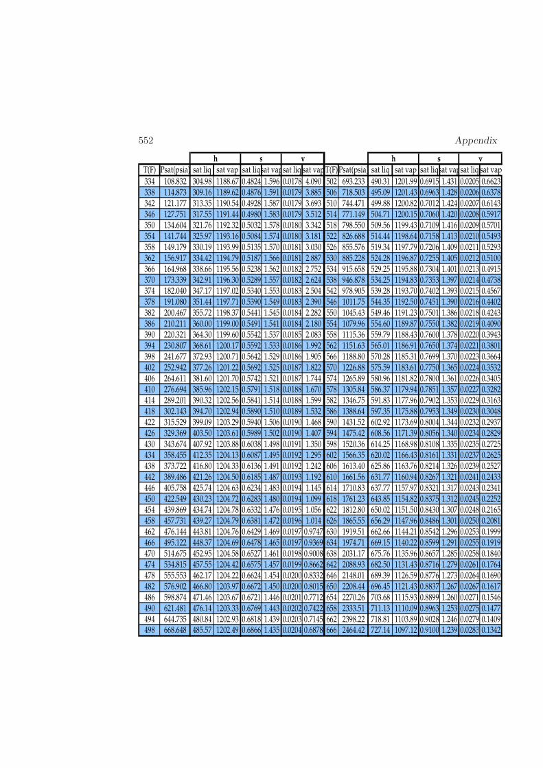
552 Appendix
T(F) Psat(psia) sat liq sat vap sat liqsat vapsat liq sat vapT(F)Psat(psia) sat liq sat vap sat liqsat vapsat liq sat vap
334 108.832 304.98 1188.67 0.4824 1.596 0.0178 4.090 502 693.233 490.31 1201.99 0.6915 1.431 0.0205 0.6623338 114.873 309.16 1189.62 0.4876 1.591 0.0179 3.885 506 718.503 495.09 1201.43 0.6963 1.428 0.0206 0.6378342 121.177 313.35 1190.54 0.4928 1.587 0.0179 3.693 510 744.471 499.88 1200.82 0.7012 1.424 0.0207 0.6143346 127.751 317.55 1191.44 0.4980 1.583 0.0179 3.512 514 771.149 504.71 1200.15 0.7060 1.420 0.0208 0.5917350 134.604 321.76 1192.32 0.5032 1.578 0.0180 3.342 518 798.550 509.56 1199.43 0.7109 1.416 0.0209 0.5701354 141.744 325.97 1193.16 0.5084 1.574 0.0180 3.181 522 826.688 514.44 1198.64 0.7158 1.413 0.0210 0.5493358 149.179 330.19 1193.99 0.5135 1.570 0.0181 3.030 526 855.576 519.34 1197.79 0.7206 1.409 0.0211 0.5293362 156.917 334.42 1194.79 0.5187 1.566 0.0181 2.887 530 885.228 524.28 1196.87 0.7255 1.405 0.0212 0.5100366 164.968 338.66 1195.56 0.5238 1.562 0.0182 2.752 534 915.658 529.25 1195.88 0.7304 1.401 0.0213 0.4915370 173.339 342.91 1196.30 0.5289 1.557 0.0182 2.624 538 946.878 534.25 1194.83 0.7353 1.397 0.0214 0.4738374 182.040 347.17 1197.02 0.5340 1.553 0.0183 2.504 542 978.905 539.28 1193.70 0.7402 1.393 0.0215 0.4567378 191.080 351.44 1197.71 0.5390 1.549 0.0183 2.390 546 1011.75 544.35 1192.50 0.7451 1.390 0.0216 0.4402382 200.467 355.72 1198.37 0.5441 1.545 0.0184 2.282 550 1045.43 549.46 1191.23 0.7501 1.386 0.0218 0.4243386 210.211 360.00 1199.00 0.5491 1.541 0.0184 2.180 554 1079.96 554.60 1189.87 0.7550 1.382 0.0219 0.4090390 220.321 364.30 1199.60 0.5542 1.537 0.0185 2.083 558 1115.36 559.79 1188.43 0.7600 1.378 0.0220 0.3943394 230.807 368.61 1200.17 0.5592 1.533 0.0186 1.992 562 1151.63 565.01 1186.91 0.7650 1.374 0.0221 0.3801398 241.677 372.93 1200.71 0.5642 1.529 0.0186 1.905 566 1188.80 570.28 1185.31 0.7699 1.370 0.0223 0.3664402 252.942 377.26 1201.22 0.5692 1.525 0.0187 1.822 570 1226.88 575.59 1183.61 0.7750 1.365 0.0224 0.3532406 264.611 381.60 1201.70 0.5742 1.521 0.0187 1.744 574 1265.89 580.96 1181.82 0.7800 1.361 0.0226 0.3405410 276.694 385.96 1202.15 0.5791 1.518 0.0188 1.670 578 1305.84 586.37 1179.94 0.7851 1.357 0.0227 0.3282414 289.201 390.32 1202.56 0.5841 1.514 0.0188 1.599 582 1346.75 591.83 1177.96 0.7902 1.353 0.0229 0.3163418 302.143 394.70 1202.94 0.5890 1.510 0.0189 1.532 586 1388.64 597.35 1175.88 0.7953 1.349 0.0230 0.3048422 315.529 399.09 1203.29 0.5940 1.506 0.0190 1.468 590 1431.52 602.92 1173.69 0.8004 1.344 0.0232 0.2937426 329.369 403.50 1203.61 0.5989 1.502 0.0190 1.407 594 1475.42 608.56 1171.39 0.8056 1.340 0.0234 0.2829430 343.674 407.92 1203.88 0.6038 1.498 0.0191 1.350 598 1520.36 614.25 1168.98 0.8108 1.335 0.0235 0.2725434 358.455 412.35 1204.13 0.6087 1.495 0.0192 1.295 602 1566.35 620.02 1166.43 0.8161 1.331 0.0237 0.2625438 373.722 416.80 1204.33 0.6136 1.491 0.0192 1.242 606 1613.40 625.86 1163.76 0.8214 1.326 0.0239 0.2527442 389.486 421.26 1204.50 0.6185 1.487 0.0193 1.192 610 1661.56 631.77 1160.94 0.8267 1.321 0.0241 0.2433446 405.758 425.74 1204.63 0.6234 1.483 0.0194 1.145 614 1710.83 637.77 1157.97 0.8321 1.317 0.0243 0.2341450 422.549 430.23 1204.72 0.6283 1.480 0.0194 1.099 618 1761.23 643.85 1154.82 0.8375 1.312 0.0245 0.2252454 439.869 434.74 1204.78 0.6332 1.476 0.0195 1.056 622 1812.80 650.02 1151.50 0.8430 1.307 0.0248 0.2165458 457.731 439.27 1204.79 0.6381 1.472 0.0196 1.014 626 1865.55 656.29 1147.96 0.8486 1.301 0.0250 0.2081462 476.144 443.81 1204.76 0.6429 1.469 0.0197 0.9747 630 1919.51 662.66 1144.21 0.8542 1.296 0.0253 0.1999466 495.122 448.37 1204.69 0.6478 1.465 0.0197 0.9369 634 1974.71 669.15 1140.22 0.8599 1.291 0.0255 0.1919470 514.675 452.95 1204.58 0.6527 1.461 0.0198 0.9008 638 2031.17 675.76 1135.96 0.8657 1.285 0.0258 0.1840474 534.815 457.55 1204.42 0.6575 1.457 0.0199 0.8662 642 2088.93 682.50 1131.43 0.8716 1.279 0.0261 0.1764478 555.553 462.17 1204.22 0.6624 1.454 0.0200 0.8332 646 2148.01 689.39 1126.59 0.8776 1.273 0.0264 0.1690482 576.902 466.80 1203.97 0.6672 1.450 0.0200 0.8015 650 2208.44 696.45 1121.43 0.8837 1.267 0.0267 0.1617486 598.874 471.46 1203.67 0.6721 1.446 0.0201 0.7712 654 2270.26 703.68 1115.93 0.8899 1.260 0.0271 0.1546490 621.481 476.14 1203.33 0.6769 1.443 0.0202 0.7422 658 2333.51 711.13 1110.09 0.8963 1.253 0.0275 0.1477494 644.735 480.84 1202.93 0.6818 1.439 0.0203 0.7145 662 2398.22 718.81 1103.89 0.9028 1.246 0.0279 0.1409498 668.648 485.57 1202.49 0.6866 1.435 0.0204 0.6878 666 2464.42 727.14 1097.12 0.9100 1.239 0.0283 0.1342
h s v h s v
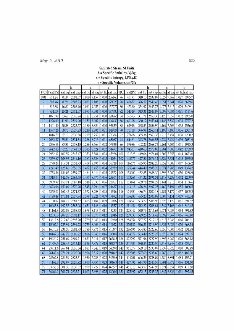
May 5, 2010 553
T(C) Psat(Pa) sat liq sat vap sat liqsat vapsat liq sat vap T(C) Psat(Pa) sat liq sat vap sat liqsat vapsat liq sat vap
0.01 611.24 0.00 2501.57 0.000 9.157 1.000 206163 76 40191 318.13 2637.07 1.027 7.669 1.027 3975.72 705.46 8.39 2505.23 0.031 9.105 1.000 179923 78 43652 326.52 2640.42 1.051 7.641 1.028 3679.64 812.88 16.80 2508.90 0.061 9.053 1.000 157272 80 47360 334.92 2643.75 1.075 7.613 1.029 3409.16 934.53 25.21 2512.57 0.091 9.001 1.000 137780 82 51329 343.31 2647.07 1.099 7.586 1.031 3161.68 1071.99 33.60 2516.24 0.121 8.951 1.000 120966 84 55573 351.71 2650.36 1.123 7.559 1.032 2935.0
10 1226.99 41.99 2519.90 0.151 8.902 1.000 106430 86 60108 360.12 2653.64 1.146 7.532 1.033 2727.212 1401.40 50.38 2523.57 0.180 8.854 1.000 93835 88 64948 368.53 2656.90 1.169 7.506 1.035 2536.514 1597.26 58.75 2527.23 0.210 8.806 1.001 82900 90 70109 376.94 2660.14 1.193 7.480 1.036 2361.316 1816.79 67.13 2530.88 0.239 8.759 1.001 73384 92 75608 385.36 2663.35 1.216 7.454 1.038 2200.218 2062.37 75.50 2534.54 0.268 8.713 1.001 65087 94 81461 393.78 2666.55 1.239 7.429 1.039 2051.920 2336.56 83.86 2538.18 0.296 8.668 1.002 57838 96 87686 402.20 2669.73 1.261 7.404 1.041 1915.322 2642.15 92.23 2541.83 0.325 8.624 1.002 51492 98 94301 410.63 2672.88 1.284 7.380 1.042 1789.324 2982.12 100.59 2545.47 0.353 8.581 1.003 45926 100 101325 419.06 2676.01 1.307 7.355 1.044 1673.026 3359.67 108.95 2549.10 0.381 8.538 1.003 41034 102 108777 427.50 2679.12 1.329 7.331 1.045 1565.528 3778.24 117.31 2552.73 0.409 8.496 1.004 36728 104 116676 435.95 2682.20 1.352 7.308 1.047 1466.230 4241.49 125.66 2556.35 0.437 8.455 1.004 32929 106 125044 444.40 2685.26 1.374 7.285 1.049 1374.232 4753.36 134.02 2559.97 0.464 8.414 1.005 29572 108 133900 452.85 2688.30 1.396 7.262 1.050 1288.934 5318.04 142.38 2563.58 0.491 8.374 1.006 26601 110 143266 461.32 2691.31 1.418 7.239 1.052 1209.936 5939.99 150.74 2567.18 0.518 8.335 1.006 23967 112 153164 469.78 2694.29 1.441 7.216 1.054 1136.638 6623.96 159.09 2570.78 0.545 8.296 1.007 21627 114 163618 478.26 2697.25 1.462 7.194 1.055 1068.540 7375.01 167.45 2574.37 0.572 8.258 1.008 19546 116 174650 486.74 2700.18 1.484 7.172 1.057 1005.242 8198.49 175.81 2577.94 0.599 8.221 1.009 17692 118 186283 495.23 2703.08 1.506 7.151 1.059 946.3444 9100.07 184.17 2581.52 0.625 8.184 1.009 16036 120 198543 503.72 2705.96 1.528 7.129 1.061 891.5246 10085.8 192.53 2585.08 0.651 8.148 1.010 14557 122 211454 512.22 2708.81 1.549 7.108 1.062 840.4548 11161.9 200.89 2588.63 0.678 8.113 1.011 13233 124 225042 520.73 2711.63 1.571 7.087 1.064 792.8350 12335.3 209.26 2592.17 0.704 8.078 1.012 12046 126 239333 529.25 2714.42 1.592 7.067 1.066 748.4052 13612.8 217.62 2595.70 0.729 8.043 1.013 10980 128 254354 537.77 2717.18 1.613 7.046 1.068 706.9154 15002.1 225.99 2599.22 0.755 8.009 1.014 10022 130 270132 546.31 2719.90 1.634 7.026 1.070 668.1456 16510.8 234.35 2602.73 0.780 7.976 1.015 9158.7 132 286696 554.85 2722.60 1.655 7.006 1.072 631.8858 18147.3 242.72 2606.22 0.806 7.943 1.016 8380.8 134 304072 563.40 2725.27 1.676 6.986 1.074 597.9560 19920.2 251.09 2609.71 0.831 7.911 1.017 7678.5 136 322292 571.96 2727.90 1.697 6.967 1.076 566.1862 21838.5 259.46 2613.18 0.856 7.879 1.018 7043.7 138 341384 580.53 2730.50 1.718 6.948 1.078 536.4164 23911.6 267.84 2616.64 0.881 7.848 1.019 6469.0 140 361379 589.10 2733.07 1.739 6.928 1.080 508.4966 26149.6 276.21 2620.08 0.906 7.817 1.020 5948.2 142 382308 597.69 2735.60 1.760 6.910 1.082 482.3068 28562.8 284.59 2623.51 0.930 7.786 1.022 5475.6 144 404201 606.29 2738.09 1.780 6.891 1.084 457.7170 31162.0 292.97 2626.92 0.955 7.756 1.023 5046.3 146 427092 614.90 2740.56 1.801 6.872 1.086 434.6072 33958.5 301.36 2630.32 0.979 7.727 1.024 4655.7 148 451013 623.52 2742.98 1.821 6.854 1.089 412.8874 36964.0 309.74 2633.71 1.003 7.698 1.025 4300.0 150 475997 632.15 2745.37 1.842 6.836 1.091 392.45
vh s
v = Specific Volume, cm^3/g
Saturated Steam: SI Units
h = Specific Enthalpy, kJ/kg
s = Specific Entropy, kJ/(kg.K)
vh s

554 Appendix
T(C) Psat(Pa) sat liq sat vap sat liqsat vapsat liq sat vap T(C) Psat(Pa) sat liq sat vap sat liqsat vapsat liq sat vap
152 502078 640.79 2747.72 1.862 6.818 1.093 373.22 236 3118600 1018.57 2802.34 2.665 6.169 1.221 64.081154 529289 649.44 2750.03 1.882 6.800 1.095 355.10 238 3231655 1028.07 2802.32 2.684 6.155 1.225 61.822156 557668 658.11 2752.30 1.902 6.782 1.098 338.03 240 3347832 1037.60 2802.21 2.702 6.141 1.229 59.654158 587247 666.79 2754.53 1.922 6.765 1.100 321.94 242 3467190 1047.17 2802.02 2.720 6.127 1.233 57.574160 618065 675.47 2756.73 1.942 6.747 1.102 306.76 244 3589787 1056.77 2801.75 2.739 6.113 1.238 55.575162 650157 684.18 2758.88 1.962 6.730 1.105 292.42 246 3715682 1066.40 2801.40 2.757 6.099 1.242 53.655164 683561 692.89 2760.99 1.982 6.713 1.107 278.89 248 3844934 1076.07 2800.96 2.775 6.085 1.247 51.811166 718314 701.62 2763.05 2.002 6.696 1.109 266.09 250 3977602 1085.78 2800.43 2.793 6.071 1.251 50.037168 754455 710.36 2765.08 2.022 6.680 1.112 254.00 252 4113749 1095.53 2799.82 2.812 6.057 1.256 48.332170 792023 719.12 2767.06 2.042 6.663 1.114 242.55 254 4253433 1105.32 2799.11 2.830 6.043 1.261 46.692172 831057 727.89 2768.99 2.061 6.647 1.117 231.72 256 4396718 1115.15 2798.31 2.848 6.029 1.266 45.114174 871597 736.67 2770.88 2.081 6.630 1.120 221.47 258 4543665 1125.03 2797.41 2.867 6.015 1.271 43.596176 913684 745.47 2772.72 2.100 6.614 1.122 211.75 260 4694337 1134.94 2796.42 2.885 6.001 1.276 42.134178 957359 754.29 2774.52 2.120 6.598 1.125 202.54 262 4848797 1144.90 2795.32 2.903 5.987 1.281 40.726180 1002663 763.12 2776.27 2.139 6.582 1.128 193.80 264 5007109 1154.91 2794.12 2.921 5.973 1.286 39.369182 1049639 771.96 2777.97 2.159 6.566 1.130 185.51 266 5169338 1164.97 2792.81 2.940 5.959 1.291 38.062184 1098330 780.83 2779.62 2.178 6.550 1.133 177.64 268 5335549 1175.07 2791.40 2.958 5.945 1.297 36.803186 1148778 789.71 2781.22 2.197 6.535 1.136 170.17 270 5505808 1185.23 2789.87 2.976 5.930 1.303 35.588188 1201028 798.60 2782.76 2.216 6.519 1.139 163.07 272 5680181 1195.44 2788.22 2.995 5.916 1.308 34.416190 1255124 807.52 2784.26 2.236 6.504 1.142 156.32 274 5858737 1205.70 2786.46 3.013 5.902 1.314 33.286192 1311110 816.45 2785.70 2.255 6.488 1.144 149.90 276 6041542 1216.02 2784.57 3.031 5.888 1.320 32.196194 1369033 825.40 2787.10 2.274 6.473 1.147 143.79 278 6228666 1226.40 2782.56 3.050 5.873 1.326 31.143196 1428938 834.37 2788.43 2.293 6.458 1.150 137.97 280 6420179 1236.84 2780.42 3.068 5.859 1.332 30.126198 1490871 843.36 2789.71 2.312 6.443 1.153 132.44 282 6616151 1247.34 2778.14 3.087 5.844 1.339 29.144200 1554880 852.37 2790.94 2.331 6.428 1.156 127.16 284 6816653 1257.90 2775.73 3.105 5.829 1.345 28.195202 1621012 861.4 2792.11 2.350 6.413 1.160 122.13 286 7021758 1268.54 2773.18 3.124 5.815 1.352 27.279204 1689315 870.5 2793.22 2.368 6.398 1.163 117.34 288 7231540 1279.24 2770.48 3.142 5.800 1.359 26.392206 1759838 879.5 2794.27 2.387 6.383 1.166 112.77 290 7446073 1290.01 2767.64 3.161 5.785 1.366 25.535208 1832629 888.6 2795.26 2.406 6.369 1.169 108.40 292 7665432 1300.86 2764.64 3.180 5.770 1.373 24.706210 1907739 897.7 2796.20 2.425 6.354 1.173 104.24 294 7889695 1311.78 2761.48 3.199 5.754 1.381 23.904212 1985217 906.9 2797.07 2.443 6.339 1.176 100.26 296 8118939 1322.79 2758.17 3.217 5.739 1.388 23.128214 2065114 916.0 2797.88 2.462 6.325 1.179 96.461 298 8353245 1333.88 2754.68 3.236 5.724 1.396 22.376216 2147480 925.2 2798.62 2.481 6.310 1.183 92.830 300 8592692 1345.05 2751.03 3.255 5.708 1.404 21.649218 2232368 934.4 2799.30 2.499 6.296 1.186 89.358 302 8837364 1356.32 2747.20 3.274 5.692 1.412 20.944220 2319830 943.7 2799.92 2.518 6.282 1.190 86.038 304 9087345 1367.69 2743.19 3.293 5.676 1.421 20.261222 2409919 952.9 2800.47 2.536 6.267 1.194 82.861 306 9342721 1379.15 2738.99 3.313 5.660 1.430 19.599224 2502686 962.2 2800.95 2.555 6.253 1.197 79.820 308 9603580 1390.72 2734.60 3.332 5.644 1.439 18.957226 2598187 971.5 2801.36 2.573 6.239 1.201 76.909 310 9870012 1402.39 2730.01 3.351 5.628 1.448 18.334228 2696475 980.9 2801.70 2.592 6.225 1.205 74.121 312 1.01E+07 1414.18 2725.21 3.371 5.611 1.458 17.730230 2797605 990.3 2801.97 2.610 6.211 1.209 71.450 314 1.04E+07 1426.09 2720.19 3.390 5.594 1.468 17.143232 2901632 999.7 2802.17 2.629 6.197 1.213 68.890 316 1.07E+07 1438.13 2714.93 3.410 5.577 1.478 16.573234 3008612 1009.1 2802.30 2.647 6.183 1.217 66.435 318 1.10E+07 1450.30 2709.43 3.430 5.560 1.488 16.019
h s v h s v
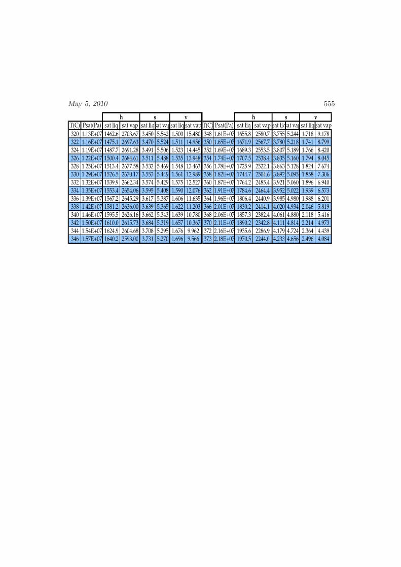
May 5, 2010 555
T(C) Psat(Pa) sat liq sat vap sat liqsat vapsat liq sat vap T(C) Psat(Pa) sat liq sat vap sat liqsat vapsat liq sat vap
320 1.13E+07 1462.6 2703.67 3.450 5.542 1.500 15.480 348 1.61E+07 1655.8 2580.7 3.755 5.244 1.718 9.178322 1.16E+07 1475.1 2697.63 3.470 5.524 1.511 14.956 350 1.65E+07 1671.9 2567.7 3.780 5.218 1.741 8.799324 1.19E+07 1487.7 2691.28 3.491 5.506 1.523 14.445 352 1.69E+07 1689.3 2553.5 3.807 5.189 1.766 8.420326 1.22E+07 1500.4 2684.61 3.511 5.488 1.535 13.948 354 1.74E+07 1707.5 2538.4 3.835 5.160 1.794 8.045328 1.25E+07 1513.4 2677.58 3.532 5.469 1.548 13.463 356 1.78E+07 1725.9 2522.1 3.863 5.128 1.824 7.674330 1.29E+07 1526.5 2670.17 3.553 5.449 1.561 12.989 358 1.82E+07 1744.7 2504.6 3.892 5.095 1.858 7.306332 1.32E+07 1539.9 2662.34 3.574 5.429 1.575 12.527 360 1.87E+07 1764.2 2485.4 3.921 5.060 1.896 6.940334 1.35E+07 1553.4 2654.06 3.595 5.408 1.590 12.076 362 1.91E+07 1784.6 2464.4 3.952 5.022 1.939 6.573336 1.39E+07 1567.2 2645.29 3.617 5.387 1.606 11.635 364 1.96E+07 1806.4 2440.9 3.985 4.980 1.988 6.201338 1.42E+07 1581.2 2636.00 3.639 5.365 1.622 11.203 366 2.01E+07 1830.2 2414.1 4.020 4.934 2.046 5.819340 1.46E+07 1595.5 2626.16 3.662 5.343 1.639 10.780 368 2.06E+07 1857.3 2382.4 4.061 4.880 2.118 5.416342 1.50E+07 1610.0 2615.73 3.684 5.319 1.657 10.367 370 2.11E+07 1890.2 2342.8 4.111 4.814 2.214 4.973344 1.54E+07 1624.9 2604.68 3.708 5.295 1.676 9.962 372 2.16E+07 1935.6 2286.9 4.179 4.724 2.364 4.439346 1.57E+07 1640.2 2593.00 3.731 5.270 1.696 9.566 373 2.18E+07 1970.5 2244.0 4.233 4.656 2.496 4.084
h s v h s v

556 Appendix

May 5, 2010 557

558 Appendix

May 5, 2010 559

560 Appendix

May 5, 2010 561

562 Appendix

May 5, 2010 563

564 Appendix

May 5, 2010 565

566 Appendix

May 5, 2010 567

568 Appendix

May 5, 2010 569

570 Appendix
Bibliography
[1] Milton Abramowitz and Irene E. Stegun. Handbook of Mathematical Func-tions. National Bureau of Standards, Washington D.C., 1964. 227, 507, 510
[2] Andrzej Anderko. Equations of State for Fluids and Fluid Mixtures, volumeExperimental Thermodynamics, Part I, chapter 4: Cubic and Generalized vander Waals Equations, pages 75–126. Elsevier, Amsterdam, 2000. 513
[3] A. J. Appleby and F. R. Foulkes. Fuel Cell Handbook. U.S. Department ofEnergy, Morgantown, West Virginia, 5th edition, October 2000. Availableonline at http://www.fuelcells.org/fchandbook.pdf. 89, 196, 197
[4] Kelyn A Arora, Alan J. Lesser, and Thomas J. McCarthy. Preparation andcharacterization of microcellular polystyrene foams processed in supercriticalcarbon dioxide. Macromolecules, 31:4614–4620, 1998. 447
[5] R. Dean Astumian and Peter Hanggi. Brownian motors. Physics Today,55(11):33–39, November 2002. 202
[6] M. Benedict, G. B. Webb, and L. C. Rubin. Chemical Engineering Progress,47:419, 1951. 525
[7] Antony N. Beris and Brian J. Edwards. Thermodynamics of Flowing Systemswith internal microstructure. Oxford University Press, New York, 1994. 179
[8] R. Byron Bird. The basic concepts in transport phenomena. Chem. Eng.Educ., Spring:102–109, 1993. 181, 532, 533
[9] R. Byron Bird, Ole Hassager, Robert C. Armstrong, and Charles F. Curtiss.Dynamics of Polymeric Liquids Vol I: Rheology. Addison-Wesley, New York,2nd edition, 1987. 535
[10] R. Byron Bird, Warren E. Stewart, and Edwin N. Lightfoot. Transport Phe-nomena. John Wiley and Sons, New York, 1960. 181, 182, 183, 529, 531, 532,533, 534, 535
571
572 Appendix
[11] Carlos Bustamante, J. F. Marko, E. D. Siggia, and S. Smith. Entropic elas-ticity of λ-phage DNA. Science, 265:1599–1600, September 1994. 59, 60,243
[12] D. Buttin, M. DuPont, M. Straumann, R. Gille, J.-C. Dubois, R. Ornelas, C.P.Fleba, E. Ramunni, V. Antonucci, A.S. Arico, P. Creti, E. Modica, M. Pham-Thi, and J.-P. Ganne. Development and operation of a 150 w air-feed directmethanol fuel cell stack. Journal of Applied Electrochemistry, 31:275–279,2001. 197
[13] Herb Callen. Thermodynamics and an Introduction to Thermostatistics. Wi-ley, New York, 2nd edition, 1985. 10, 12, 71, 95, 137, 222
[14] David Chandler. Introduction to Modern Statistical Mechanics. Oxford, NewYork, 1987. 279, 281
[15] M. W. Chase, Jr., C. A. Davies, J. R. Downey, Jr., D. J. Frurip, R. A. Mc-Donald, and A. N. Syverud. JANAF thermochemical tables, 3rd ed. J. Phys.Chem. Ref. Data, 14, 1985. Supplement No. 1. 89, 197, 402, 544, 545
[16] S.J. Chen and M. Radosz. Saft. Macromolecules, 25:3089–????, 1992. 277
[17] N. Choudhury and B. M. Pettitt. On the mechanism of hydrophobic associa-tion of nanoscopic solutes. J. Am. Chem. Soc., 127:3556–3567, 2005. 281
[18] Rudolf Clausius. Uber den zweiten Hauptsatz der MechanischenWarmetheorie. Friedrich Vieweg und Sohn, Braunschweig, Germany, 1867.24
[19] Kenny Keith Crain. An investigation of the benedict-webb-rubin equation.Masters of engineering, University of Louisville, August 1972. 525
[20] C. Danilowicz, Y. Kafri, R. S. Conroy, V.W. Coljee, J.Weeks, and M. Prentiss.Measurement of the phase diagram of dna unzipping in the temperature-forceplane. Phys. Rev. Letters, 93(7):078101, August 2004. 102, 103
[21] Michel Daune. Molecular Biophysics: Structures in motion. Oxford UniversityPress, Oxford, 2003. 409
[22] S. R. de Groot and P. Mazur. Non-Equilibrium Thermodynamics. DoverPublications, New York, 1984. 536, 537
[23] John A. Dean, editor. Lange’s Handbook of Chemistry. McGraw-Hill, NewYork, 12th edition, 1978. 546, 547
May 5, 2010 573
[24] J. H. Dymond and E. B. Smith. The Virial Coefficients of Pure Gases andMixtures. Clarendon Press, Oxford, 1980. 516
[25] J.H. Dymond and E.B. Smith. The Virial Coefficients of Gases: a CriticalCompilation. Clarendon Press, Oxford, 1969. 275
[26] Carl Eckert. The thermodynamics of irreversible processes. Phys. Rev.,58:267–269, 1940. 534
[27] Fernando A. Escobedo, S. Nath, and Juan Jose de Pablo. On the simulationof phase equilibria alkanes. J. Chem. Phys., ??:???–???, 1998. 265
[28] R. M. Felder and R. W. Rousseau. Elementary Principles of Chemical Pro-cesses. John Wiley & Sons, New York, 2nd edition, 1986. 182, 332, 525
[29] John L. Ferry. Viscoelastic Properties of Polymers. John Wiley & Sons, NewYork, 3rd edition, 1980. 458
[30] Richard P. Feynman, Robert B. Leighton, and Matthew Sands. The Feyn-man Lectures on Physics: Volume I. Mainly mechanics, radiation and heat.Addison-Wesley, Reading, Massachusetts, 1963. 220
[31] Paul J. Flory. Principles of Polymer Chemistry. Cornell University, Ithaca,1953. 458
[32] Paul J. Flory. Statistical Mechanics of Chain Molecules. Hanser, Munich,1988. 458
[33] H. Scott Fogler. Elements of Chemical Reaction Engineering. Prentice Hall,3rd edition, 1998. 391
[34] R. H. Fowler and E. A. Guggenheim. Statistical Thermodynamics. CambridgeUniversity Press, Cambridge, 1939. 127
[35] A. Garg, Esin Gulari, and Charles W. Manke. Thermodynamics of polymermelts swollen with supercritical gases. Macromolecules, 27:5643–53, 1994. 450
[36] J.G. Gay and B.J. Berne. J. Chem. Phys., 74:3316–????, 1981. 286
[37] J. Gross, O. Spuhl, F. Tumakaka, and G. Sadowski. Modeling copolymersystems using the perturbed-chain saft equation of state. Industrial & Engi-neering Chemistry Research, 42(6):1266–1274, 2003. 442
[38] A. F. Gutsol. The Ranque effect. Physics-Uspekhi, 40(6):639–658, 1997. 191,194
574 Appendix
[39] Ernest J. Henly and E. M. Rosen. Material and Energy Balance Computations.Wiley, New York, 1969. Is this the most up-to-date edition? Info correct? 525
[40] Tomaz Heyduk and James C. Lee. Application of fluourescence energy transferand polarization to monitor escherichia coli camp receptor protein and lacpromotor interaction. Proc. Nat. Acad. Sci., 87:1744–1748, 1990. 111, 112
[41] P.C. Hiemenz and Raj Rajagopalan. Principles of Colloid and Surface Chem-istry. Marcel Dekker, New York, 1997. 124
[42] Terrel L. Hill. An Introduction to Statistical Thermodynamics. Dover, NewYork, 1986. 108, 233
[43] Terrell L. Hill. Thermodynamics of Small Systems, volume I and II. Dover,New York, 1963–1964. 44
[44] Rudolph Hilsch. The use of the expansion of gases in a centrifugal field as acooling process. The Review of Scientific Instruments, 18(2):108, 1947. 191
[45] D. M. Himmelblau. Basic Principles and Calculations in Chemical Engineer-ing. Prentice Hall PTR, Upper Saddle River, New Jersey, 6th edition, 1996.182
[46] Joseph O. Hirschfelder, Charles F. Curtiss, and Robert B. Bird. MolecularTheory of Gases and Liquids. John Wiley and Sons, New York, 1954. 257
[47] Joseph Honerkamp. Stochastische Dynamische Systeme. VCH, Berlin, 1983.417
[48] X. H. Huang, R. H. Zhou, and B. J. Berne. Drying and hydrophobic collapseof paraffin plates. J. Phys. Chem. B, 109:3546–3552, 2005. 281
[49] Johnson, Zollweg, and Gubbins. Molecular Physics, 78:591–618, 1993. 524
[50] Susan Kapsabelis and Clive A. Prestidge. Adsorption ofethyl(hydroxylethyl)cellulose onto silica particles: The role of surfacechemistry and temperature. J.Colloid Interfacial Sci., 228:297–305, 2000. 126
[51] A. I. Khinchin. Mathematical foundations of information theory. Dover Pub-lications, Inc., New York, 1957. 224
[52] A. Ya. Kipnis, B. E. Yavelov, and John S. Rowlinson. Van der Waals andMolecular Science. Clarendon Press, Oxford, 1996. 516
May 5, 2010 575
[53] D. Kondepudi and I. Prigogine. Modern Thermodynamics: From Heat Enginesto Dissipative Structures. Wiley, Chichester, 1998. 537
[54] H. Kreuzer. Nonequilibrium Thermodynamics and its Statistical Foundations.Clarendon Press, Oxford, 1981. 537
[55] Stephen M. Lambert, Yuhua Song, and John M. Prausnitz. Equations of Statefor Fluids and Fluid Mixtures, Part II, chapter Equations of State for PolymerSystems, pages 523–588. Experimental Thermodynamics, Volume V. Elsevier,Amsterdam, 2000. 448
[56] G.C. Maitland, M. Rigby, E. Brian Smith, andW.A. Wakeham. IntermolecularForces. Clarendon Press, Oxford, 1981. 259
[57] John F. Marko and Eric D. Siggia. Stretching DNA. Macromolecules, 28:8759–8770, 1995. 60, 239
[58] Kurt H. Meyer and Cesare Ferri. Sur l’elasticite du caoutchouc. Helv. Chim.Acta, 18:570–589, 1935. 99
[59] Michael Modell and Robert C. Reid. Thermodynamics and Its Applications.Prentice-Hall, Englewood Cliffs, N.J., 2nd edition, 1983. 71
[60] P.S. Murte and M. van Winkle. Chem.Eng.Data Ser., 3:72, 1978. 386
[61] Hossein Naghibi, Atsuo Tamura, and Julian M. Sturtevant. Significant dis-crepancies between van’t hoff and calorimetric enthalpies. Proc. Nat. Acad.Sci., 92:5597–5599,, 1995. 427, 428
[62] W. Nernst. The New Heat Theorem. Dutton, New York, 1926. 24
[63] Friedrich Nietzsche. Daybreak: Thoughts on the Prejudices of Morality. Cam-bridge University Press, Cambridge, UK, 1997. translated by R. J. Hollingdale.133
[64] Hans Christian Ottinger. Beyond Equilibrium Thermodynamics. Wiley-Interscience, Hoboken, NJ, 2005. 179, 224
[65] A.Z. Panagiotopoulos. Simulations of phase equilibria in the Gibbs ensemble.Mol. Phys., ??:???–???, 1989. 265
[66] C. Panayiotou and Isaac Sanchez. Statistical thermodynamics of associatedpolymer solutions. Macromolecules, 24:6231–6237, 1991. 468
576 Appendix
[67] William M. Pardridge. Cns drug design based on principles of blood-brainbarrier transport. J Neurochem, 70(5):1781–1781, 1998. 364
[68] William M. Pardridge. Brain drug targeting. Cambridge, Cambridge, UK,2001. 364
[69] Kenneth S. Pitzer. Thermodynamics. McGraw-Hill, New York, 3rd edition,1995. 9, 230, 515, 526, 546
[70] Bruce E. Poling, John M. Prausnitz, and John P. O’Connell. The Propertiesof Gases and Liquids. McGraw-Hill, New York, 5th edition, 2001. 344
[71] Bruce E. Poling, John M. Prausnitz, and John P. O’Connell. The Propertiesof Gases and Liquids. McGraw-Hill, New York, 5th edition, 2001. 513, 514,546
[72] W. H. Press, S. A. Teukolsky, W. T. Vetterling, and B. P. Flannery. NumericalRecipes in FORTRAN: The Art of Scientific Computing, 2nd ed. CambridgeUniversity Press, Cambridge, 2nd edition, 1992. 98, 99, 224, 406, 445
[73] Caiban Qian, Stephen J. Mumby, and B. E. Eichinger. Phase diagrams ofbinary polymer solutions and blends. Macromolecules, 24(7):1655–1661, 1991.442, 443, 467
[74] Georges Ranque. Experiences sur la detente giratoire avec productions simul-tanees d’un enchappement d’air froid. Journal de Physique et de la Radium,4:1125–1155, 1933. 191
[75] James B. Rawlings and John G. Ekerdt. Chemical Reactor Analysis and De-sign Fundamentals. Nob Hill Publishing, Madison, Wisconsin, 2002. 391,413
[76] Otto Redlich and J. N. S. Kwong. On the thermodynamics of solutions. V Anequation of state. Fugacities of gaseous solutions. Chem. Rev., 44:233–244,1949. 519
[77] R. A. Robinson and D. A. Sinclair. J.Am.Chem.Soc., 56:1830, 1934. 386
[78] Patrick A. Rodgers. Pressure-volume-temperature relationships for polymericliquids: A review of equations of state and their characteristic parameters for56 polymers. J. App. Polym. Sci., 48:1061–1080, 1993. 449
[79] Michael Rubinstein and Ralph Colby. Polymer Physics. Oxford UniversityPress, Oxford, 2003. 239
May 5, 2010 577
[80] Douglas M. Ruthven, Shamsuzzaman Farooq, and Kent S. Knaebel. PressureSwing Adsorption. VCH Publishers, New York, 1994. 107, 125
[81] Isaac C. Sanchez and Robert H.Lacombe. Statistical thermodynamics of poly-mer solutions. Macromolecules, 11:1145–1156, 1978. 448
[82] Yoshiyuki Sato, Koji Fujiwara, Tadao Takikawa, Sumarno, Shigeki Takishima,and Hirokatsu Masuoka. Solubilities and diffusion coefficients of carbon dioxideand nitrogen in polypropylene, high density polyethylene, and polystyreneunder high pressures and temperatures. Fluid Phase Equilibria, 162:261–276,1999. 449, 450
[83] Yoshiyuki Sato, M. Yurugi, Koji Fujiwara, Shigeki Takishima, and HirokatsuMasuoka. Solubilities of co2 and n2 in polystyrene under high temperatureand pressure. Fluid Phase Equilibria, 125:129–138, 1996. 450
[84] G. Schmidt and H. Wenzel. A modified van der Waals type equation of state.Chem. Eng. Sci., 35:1503–1512, 1980. 523
[85] B. Schwager, L. Chudinovskikh, A. Gavriliuk, and R. Boehler. Melt-ing curve of H2O to 90 GPa measured in a laser-heated diamond cell.J.Phys:Condens.Matter, 16:S1177–S1179, 2004. 154
[86] Jan V. Sengers, R. F. Kayser, C.J. Peters, and H.J. White. Equations of Statefor Fluids and Fluid Mixtures. Elsevier, Amsterdam, 2000. 513
[87] Johanna Levelt Sengers. How fluids unmix: Discoveries by the School of Vander Waals and Kamerlingh Onnes, volume 4 of History of Science and Schol-arship in the Netherlands. Royal Netherlands Academy of Arts and Sciences,Amsterdam, 2002. 514, 516
[88] Johanna Levelt Sengers and Antonius H. M. Levelt. Diederek Korteweg, pio-neer of criticality. Physics Today, 55(12):47–53, December 2002. 143
[89] A. N. Shaw. Phil.Trans.Royal Soc.London A, 234:299, 1935. 502
[90] Paul J. Sides. Scaling of differential equations: Analysis of the fourth kind.Chem. Eng. Educ., 36(3):232–235, 2002. 183
[91] D.A. Sinclair. J.Phys.Chem., 37:495, 1933. 386
[92] Steven B. Smith, Yujia Cui, and Carlos Bustamante. Overstretching B-DNA:The elastic response of individual double-stranded and single-stranded DNAmolecules. Science, 271:795–799, 1996. 104
578 Appendix
[93] G. Soave. Rigorous and simplified procedures for determining the pure-component parameters in the Redlich-Kwong equation of state. Chem. Eng.Sci., 35:1725–1729, 1980. 519
[94] C. L. Stong. The amateur scientist: Some delightful engines driven by theheating of rubber bands. Scientific American, 224(4):119–122, April 1971.202
[95] G.J Su and D.S. Viswanath. Generalized thermodynamic properties of realgases. I - Generalized PVT behavior of real gases (Generalized compressibilityvalues at reduced temperature and pressure ranges of real gases compared toexisting charts). AIChE J., 11:202–204, 1965. 525
[96] M. Tambasco and J.E.G. Lipson. Analyzing and predicting polymer fluidand blend properties using minimal pure component data. Macromolecules,38(7):2990–2998, 2005. 455, 457
[97] A. S. Teja, S. I. Sandler, and N. C. Patel. A generalization of the correspondingstate principle using two nonspherical reference fluids. Chem.Eng.J., 21:21–28,1981. 174
[98] Jefferson W. Tester and Michael Modell. Thermodynamics and Its Applica-tions. Prentice Hall, Upper Saddle River, New Jersey, 3rd edition, 1996. 71
[99] L. R. G. Treloar. The Physics of Rubber Elasticity. Clarendon Press, Oxford,2nd edition, 1958. 45, 128
[100] J. P. M. Trusler. Equations of State for Fluids and Fluid Mixtures, volumeExperimental Thermodynamics, Part I, chapter 3: The Virial Equation ofState, pages 35–74. Elsevier, Amsterdam, 2000. 515
[101] Patrick T. Underhill and Patrick S. Doyle. Development of bead-spring poly-mer models using the constant extension ensemble. J. Rheol., 49(5):963–987,2005. 61
[102] Johannes Diderik van der Waals. On the continuity of the gaseous and liquidstates. Studies in Statistical Mechanics, 14, 1988. translated by John ShipleyRowlinson. 141, 516
[103] Nico G. van Kampen. Stochastic Processes in Physics and Chemistry. North-Holland, Amsterdam, 1992. 392, 413, 417
[104] K. Yoshimoto, M. P. Stoykovich, H. B. Cao, J. J. de Pablo, P. F. Nealey,and W. Drugan. A two-dimensional model of the deformation of photoresist
May 5, 2010 579
structures using elastoplastic polymer properties. J. Appl. Phys., 96:1857–1865, 2004. 482
[105] Bruno H. Zimm and J. K. Bragg. J. Chem. Phys., 28:1247, 1958. 430
[106] Bruno H. Zimm and J. K. Bragg. J. Chem. Phys., 30:271, 1959. 430

580 Appendix

581
Index
acentric factor
definition, 515
activity, 397
adiabatic wall, 14
Amagat’s Law, 299
ammonia, PH diagram, 212
Anderko-Pitzer equation of state, 526
Antoine equation, 153
Avogadro’s number, 45, 549
balance, macroscopic . . . , see macroscopic. . . balance
balance, microscopic . . . , see microscopic. . . balance
Benedict-Webb-Rubin
equation of state, 54, 524–526
general
fundamental Helmholtz relation, 117
binodal curve, 133, 151
global stability criteria, 145
van der Waals fluid, 145–151
binomial coefficient, 510
binomial theorem, 509
block copolymer, 456
Boltzmann constant, 25, 103, 105, 549
calculus, fundamental theorem of , 505
calorimeter, differential scanning, 85
canonical independent variable, 67
Carnahan-Starling
critical compressibility factor, 518
critical point, 173
equation of state, 53, 518generalfundamental Helmholtz relation, 116
chain rule, 501chemical potential
and mass flows, 44
definition, 28, 29definition, alternative, 30
Clapeyron equation, 152
closed system, 14coefficient of thermal expansion
definition, 85
van der Waals, simple, 120Combinatorics, 509compressibility
isentropic, 121compressibility factor, 144, 163constant-pressure heat capacity
definition, 85ideal gas, general, 86stability criteria, 140
constant-volume heat capacitydefinition, 97ideal gas, 158ideal gas, simple, 121
stability criteria, 138–140, 170van der Waals, simple, 120
contact angle, 478
Continuity equation, 531continuity equation for a species, 531cooperativity, 411
copolymer, block, 456
582
May 5, 2010 583
corresponding states, 144, 267
Coulombic Forces, 257
critical
compressibility factor
Carnahan-Starling, 518
definition, 144
Martin’s generalized cubic, 523
Peng-Robinson, 521
Redlich-Kwong, 520
van der Waals fluid, 144
isotherm, 143
point, 143, 151
Carnahan-Starling, 173
Martin’s generalized cubic, 173
Peng-Robinson, 173
Redlich-Kwong, 172
van der Waals fluid, 143–144
pressure, 143
temperature, 143
volume, 143
cubic equations, 507
cycle
Carnot, 200
power, 202
refrigeration, 207
cyclic relation, 505
de Broglie thermal wavelength, 227
degrees of freedom, 11
delta function, 510
denaturation, 409, 410
diathermal wall, 14
differential
imperfect, 13
perfect, 13
dipole moment, 259
Dipole-ion interactions, 260
dispersion energy, 262
DNA, unzipping, 101
electron charge, 549endothermic reaction, 399energy
fundamental relation, 22internal, 11kinetic, 6, 11, 12, 182potential, 5, 11, 12, 182total, 182
energy balance, macroscopic, see macro-scopic energy balance
energy balance, microscopic, see micro-scopic energy balance
ensemblecanonical, 221grand canonical, 234microcanonical, 220
enthalpy, 67definition, 67
entropie, 24entropy
fundamental relation, 22properties, 21–22second law, 19–28stability criteria, local, 136–138
entropy balance, macroscopic, see macro-scopic entropy balance
entropy balance, microscopic, see micro-scopic entropy balance
equation of state, 17Benedict-Webb-Rubin, see Benedict-
Webb-Rubin, equation of stateCarnahan-Starling, see Carnahan-Starling,
equation of statedefinition, 29Martin’s generalized cubic, see Mar-
tin’s generalized cubic, equationof state
mechanical, 29Peng-Robinson, see Peng-Robinson,
equation of state
584 Appendix
Redlich-Kwong, see Redlich-Kwong,equation of state
Sanchez-Lacombe, see Sanchez-Lacombe,equation of state
thermal, 29
van der Waals, see van der Waals,equation of state
equilibriumstate, 18–19
equilibrium constantdefinition, 398
estimating, 400equilibrium constant(s), 391
Euler relation, 70exothermic reaction, 399
extensive variable, 11, 21extent of reaction, 394
definition, 395
Faraday’s constant, 196, 549
first lawpostulate, 11
Flory-Huggins theory, 436derivation from statistical mechan-
ics, 460
generalized, 441spinodal curve, 439
fluid, 141Fourier’s Law, 182, 537
free energy, see potential, Helmholtzfree energy, Gibbs, see potential, Gibbs
freedomdegrees of, see degrees of freedom
fuel cell, 182hydrogen, 87–92
methanol, 120fugacity, 296
coefficient, definition, 308pure, measuring, 309
definition, 307
fundamental theorem of calculus, 505
Gauss Divergence Theorem, 506General Ideal Gas, 514generalized potential
stability criteria, local, 139–140Gibbs
potential, see potential, GibbsGibbs free energy, see potential, GibbsGibbs-Duhem equation, 302
surface analog, 472Gibbs-Duhem relation, 70
heat, 13definition, 13
heat capacityconstant-pressure, see constant-pressure
heat capacityconstant-volume, see constant-volume
heat capacityheat capacity, constant volume
stability, 138heat reservoir, 73Helmholtz potential, see potential, Helmholtzhydrogen bonding, 154
ideal gasconstant-volume heat capacity, 158generalconstant-pressure heat capacity, 86fundamental Helmholtz relation, 71
isentropic process, 33–34simple, 32, 224constant-volume heat capacity, 121fundamental enthalpy relation, 116fundamental Helmholtz relation, 67–68
fundamental relation, 32statistical mechanics, 228
ideal gas constant, 549ideal gas, general, 228
May 5, 2010 585
Induced dipoles, 261
intensive variable, 29
interfaces
in mixtures, 486vapor-liquid, 486
interfacial tension, 470
internal energy, 11
stability criteria, local, 138–139Inverse Langevin force law, 239, 244
isentropic
compressibility
stability criteria, 139, 140, 170definition, 32
equivalence to adiabatic, quasi-staticprocess, 34
process, ideal gas, 33–34
process, van der Waals gas, 35isentropic compressibility, 121
iso-entergetic, 52
isobaric, 37
isochoric, 40
isolated system, 14isometric mixing, 299
isothermal compressibility
definition, 85
Peng-Robinson, 120Redlich-Kwong, 120
stability criteria, 140, 170
Jacobian transformation
definition, 502
properties, 503
Joule-Thomson coefficient, 121
Langmuir adsorption, 106, 123, 231
Langmuir adsorption isotherm, 109Laplacian, definition, 532
LeChatelier’s Principle, 399
Legendre transform, 67
inverting, 67, 102, 127
Leibniz Rule, 505
lever rule, 150
Lewis mixture, 299, 318
Lineweaver-Burke plot, 408
liquid-vapor saturation line, see binodalcurve
local equilibrium approximation, 179, 181,185, 194, 529, 533, 534, 536
macroscopic energy balance, 181
macroscopic entropy balance, 183
macroscopic mass balance, 181
Madelung’s constant, 258
Martin’s generalized cubic
critical compressibility factor, 523
critical point, 173
equation of state, 53, 522–523
general
fundamental Helmholtz relation, 117
Massieu functions, 71
matrix model, 423
Maxwell relations, 80–82
mechanical equation of state, 29
Michaelis-Menten Equation, 408
microcanonical ensemble, 220
microphase separation, 457
microscopic energy balance, 533
microscopic entropy balance, general, 536,540
microscopic entropy balance, simplified,535
microscopic internal energy balance, 533
microscopic mass balance, 531
microscopic mechanical energy balance,532
Mixture of Ideal Gases, 297
molar property, 21
multinomial coefficient, 510
multinomial theorem, 510
586 Appendix
nabla, definition, 531
Navier-Stokes equation, 532
Newtonian fluid, 532nucleation parameter, 410, 421
osmotic pressure, 360
partial molar properties, 296, 298
partial pressure, 308
partition function
canonical, 223microcanonical, 220, 223
PCR, 409
Peng-Robinson
criticalcompressibility factor, 521
critical point, 173
equation of state, 53, 520–522
generalfundamental Helmholtz relation, 117
isothermal compressibility, 120
performance, coefficient of
power cycle, 201
refrigeration cycle, 202Permanent Dipoles, 259
polarizability, 261
polymerase chain reaction, 409, 412
postulateapproach, 10–11
equilibrium, 19
first law, 11
Nernst, 24second law, 21, 23
statistical, first, 218
statistical, second, 220
potentialchemical, see chemical potential
generalized thermodynamic, 64
Gibbs
definition, 67
Helmholtz, 67definition, 67
Poynting correction, 311pressure
and volume changes, 43–44definition, 28, 29definition, alternative, 30
pressure-swing adsorption, 106process
quasi-static, 19properties, physical, 541
quasi-static process, 19
random phase approximation, 377reaction coordinate, 392Redlich-Kister expansion, 347Redlich-Kwong
critical compressibility factor, 520critical point, 172equation of state, 52, 519–520generalfundamental Helmholtz relation, 116
isothermal compressibility, 120reduced variables
definition, 144reservoir, heat, 73Residual Partial Molar Quantities, 305residual property, 161
definition, 162Reynolds transport theorem, 506rubber band
simple, ideal, 45rule
lever, 150
Sanchez-Lacombeequation of state, 447–448
saturation pressure, 146, 147sec:standard property change, 398second-order derivative, 84
May 5, 2010 587
simple van der Waals fluid, 85simple ideal gas, see ideal gas, simplespecific property, 21spinodal curve, 133, 151
Flory-Huggins theory, 439van der Waals fluid, 142–143
squarethermodynamic, 82
stability criteria, 134constant-pressure heat capacity, 140constant-volume heat capacity, 138–
140, 170global, 134binodal curve, 145
isentropic compressibility, 139, 140,170
isothermal compressibility, 140, 170local, 134entropy, 136–138generalized potential, 139–140internal energy, 138–139
standard Gibbs free energy change of re-action
definition, 398state
equation of, see equation of stateequilibrium, see equilibrium, state
statescorresponding, 144
stoichiometric coefficient, 394stress tensor, 532structure, 9substantial derivative, definition, 532supercritical fluid, 143Surface tension
temperature dependence, 484system
closed, 14isolated, 14open, 14
Taylor’s series expansion, 499
temperatureand heat flow, 39–41
definition, 28, 29definition, alternative, 30
theorem of calculus, fundamental, 505thermal conductivity, 182thermal equation of state, 29
thermodynamic square, 82Thomson equation, 477
throttling process, 177
van der Waalscritical point, 143
equation of statereduced form, 144
generalfundamental Helmholtz relation, 116
isothermal compressibility, 85
reduced form, 170simple
coefficient of thermal expansion, 120constant-volume heat capacity, 120
equation of state, 30–31fundamental relation, 26–28
spinodal curve, 143van der Waals Fluid, 517
van der Waals fluid, 516binodal curve, 145–151
critical compressibility factor, 144critical point, 144
derivation of fundamental relation, 156generalderivation of fundamental relation,158
spinodal curve, 142–143van Laar model, 349
variablecanonical independent, 67
extensive, 11, 21
588 Appendix
intensive, 29vector differential operator, definition, 531virial
mixtures, fugacity, 313Virial equation of state, 165virial equation of state, 514–516
wall, 13adiabatic, 14diathermal, 14
websites, 541
Young-Laplace equation, 474
Zimm-Bragg Matrix Model, 423zipper model, 409