chemical fate prediction for use in geo- referenced environmental
TRANSCRIPT

FACULTEIT LANDBOUWKUNDIGE ENTOEGEPASTE BIOLOGISCHE
WETENSCHAPPEN
Academiejaar 1998-1999
CHEMICAL FATE PREDICTION FOR USE IN GEO-REFERENCED ENVIRONMENTAL EXPOSURE ASSESSMENT
VOORSPELLING VAN HET GEDRAG VAN CHEMICALIENIN HET MILIEU MET HET OOG OP GEOGRAFISCH
GEREFEREERDE BLOOTSTELLINGSBEOORDELING
door
ir. Geert BOEIJE
Thesis submitted in fulfillment of the requirementsfor the degree of Doctor (Ph.D) in Applied Biological Sciences
Proefschrift voorgedragen tot het bekomen van de graadvan Doctor in de Toegepaste Biologische Wetenschappen
op gezag van
Rector: Prof. Dr. ir. J. WILLEMS
Decaan: Promotoren:
Prof. Dr. ir. O. VAN CLEEMPUT Prof. Dr. ir. P. VANROLLEGHEM
Dr. ir. D. SCHOWANEK

- i -
25.3.1999
The author and the promoters give the authorization to consult and to copy parts of this work for
personal use only. Any other use is limited by the Laws of Copyright. Permission to reproduce any
material contained in this work should be obtained from the author.
De auteur en de promotoren geven de toelating dit doctoraatswerk voor consultatie beschikbaar te
stellen, en delen ervan te copiëren voor persoonlijk gebruik. Elk ander gebruik valt onder de
beperkingen van het auteursrecht, in het bijzonder met betrekking tot de verplichting uitdrukkelijk
de bron te vermelden bij het aanhalen van de resultaten van dit werk.
De promotoren: De auteur:
Prof. Dr. ir. Peter Vanrolleghem
Dr. ir. Diederik Schowanek ir. Geert Boeije

- ii -
The research reported in this dissertation was conducted at the Department of Applied Mathematics,
Biometrics and Process Control (BIOMATH) and partly at the Laboratory of Microbial Ecology of
the University of Gent, Belgium.

- iii -
Acknowledgment
I would like to express my gratitude to all who contributed, directly or indirectly, to the realization
of this thesis.
This research was made possible by the financial support of the Environmental Risk Assessment
Steering Committee (ERASM) of the Association Internationale de la Savonnerie, de la Détergence
et des Produits d’Entretien (AISE) and the Comité Européen des Agents de Surface et
Intermédiaires Organiques (CESIO), of Procter & Gamble Eurocor, and of the United Kingdom
Environment Agency.

- iv -
Contents
Chapter 1 Geo-referenced Environmental Risk Assessment, the GREAT-ER Project
Chapter 2 A Geo-referenced Aquatic Exposure Prediction Methodology
for ‘Down-the-Drain’ Chemicals
Chapter 3 Geo-referenced Prediction of Environmental Concentrations of Chemicals
in Rivers: a Hypothetical Case Study
Chapter 4 Adaptation of the CAS Test System and Synthetic Sewage
for Biological Nutrient Removal
Chapter 5 Adaptation of the SimpleTreat Chemical Fate Model to Single-Sludge
Biological Nutrient Removal Waste Water Treatment Plants
Chapter 6 Measuring the Fate of LAS in a Pilot-Scale Trickling Filter
Chapter 7 A Steady-State Non-Equilibrium Chemical Fate Model for Trickling Filters
Chapter 8 Modeling Chemical Fate in Rivers
Chapter 9 Fate of Biodegradable Chemicals in the Sewer: Case Study for LAS
Chapter 10 New PEC Definitions for River Basins Applicable to GIS-based Environmental
Exposure Assessment
Chapter 11 Conclusions and Perspectives
References
Notation
Summary - Samenvatting
Curriculum Vitae

Chapter 1 -
Geo-referenced Environmental Risk Assessment,the GREAT-ER Project
parts of this chapter were published in:
Feijtel, T.C.J., Boeije, G., Matthies, M., Young, A., Morris, G., Gandolfi, C., Hansen, B., Fox, K.,Holt, M., Koch, V., Schröder, R., Cassani, G., Schowanek, D., Rosenblom, J. & Niessen, H. (1997).Development of a Geography-referenced Regional Exposure Assessment Tool for European Rivers -GREAT-ER. Chemosphere, 34(11), 2351-2374.

- 1.1 -
Chapter 1
Geo-referenced Environmental Risk Assessment,the GREAT-ER Project
The work described in this thesis was conducted in the framework of the GREAT-ER project
(Geography-referenced Regional Exposure Assessment Tool for European Rivers). The objective
of this international project was to develop a tool to accurately predict chemical exposure in the
aquatic environment, for use in environmental risk assessment. As the techniques which are
currently used to assess regional exposure do not account for spatial and temporal variability, and do
not offer realistic predictions of actual concentrations, they are merely applicable on a screening
level. In GREAT-ER, a software system was developed to predict concentrations of ‘down-the-
drain’ chemicals (e.g. detergents) in surface waters in a more realistic and accurate way. To reach
this objective, a Geographic Information System (GIS) was used for data storage and visualization,
combined with adequate mathematical models for the prediction of chemical fate.
1. Introduction
1.1. Safety Aspects of ‘Down-the-Drain’ Chemicals
During the past decades, households have become more and more dependent on consumer
chemicals for hygiene and comfort. In first instance, the main safety aspects of these chemicals are
related to the potential dangers they may pose to the consumer, either through normal use or through
abnormal or accidental contacts with the products.
After consumption, many of these chemical substances are discharged ‘down the drain’ into
domestic sewage (e.g. Woltering et al., 1987). During their conveyance through sewers and
purification in waste water treatment plants (WWTPs), they may be transformed or eliminated by
several chemical, biological or physical processes. However, a fraction of the chemicals - or their
transformation products - may pass through the waste water infrastructure, and be discharged into
surface waters. Another fraction can be retained in waste water treatment sludge, and may hence
end up in agricultural soil or landfills, and later be transported to ground water. Yet another fraction
may volatilize and undergo atmospheric transport, fate and deposition processes.
Chapter 1
- 1.2 -
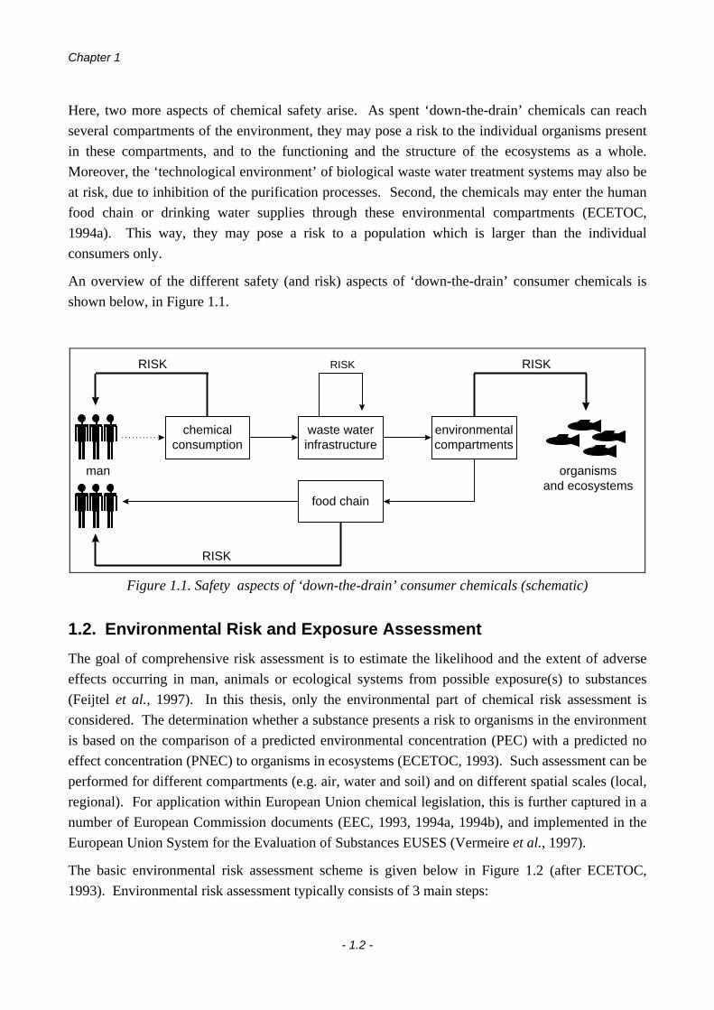
Here, two more aspects of chemical safety arise. As spent ‘down-the-drain’ chemicals can reach
several compartments of the environment, they may pose a risk to the individual organisms present
in these compartments, and to the functioning and the structure of the ecosystems as a whole.
Moreover, the ‘technological environment’ of biological waste water treatment systems may also be
at risk, due to inhibition of the purification processes. Second, the chemicals may enter the human
food chain or drinking water supplies through these environmental compartments (ECETOC,
1994a). This way, they may pose a risk to a population which is larger than the individual
consumers only.
An overview of the different safety (and risk) aspects of ‘down-the-drain’ consumer chemicals is
shown below, in Figure 1.1.
chemicalconsumption
RISK
waste waterinfrastructure
environmentalcompartments
RISK
man organismsand ecosystems
RISK
food chain
RISK
Figure 1.1. Safety aspects of ‘down-the-drain’ consumer chemicals (schematic)
1.2. Environmental Risk and Exposure Assessment
The goal of comprehensive risk assessment is to estimate the likelihood and the extent of adverse
effects occurring in man, animals or ecological systems from possible exposure(s) to substances
(Feijtel et al., 1997). In this thesis, only the environmental part of chemical risk assessment is
considered. The determination whether a substance presents a risk to organisms in the environment
is based on the comparison of a predicted environmental concentration (PEC) with a predicted no
effect concentration (PNEC) to organisms in ecosystems (ECETOC, 1993). Such assessment can be
performed for different compartments (e.g. air, water and soil) and on different spatial scales (local,
regional). For application within European Union chemical legislation, this is further captured in a
number of European Commission documents (EEC, 1993, 1994a, 1994b), and implemented in the
European Union System for the Evaluation of Substances EUSES (Vermeire et al., 1997).
The basic environmental risk assessment scheme is given below in Figure 1.2 (after ECETOC,
1993). Environmental risk assessment typically consists of 3 main steps:

Geo-referenced Environmental Risk Assessment, the GREAT-ER Project
- 1.3 -
• On the exposure side, a prediction is made of the chemical concentrations in the environmental
compartment(s) of concern (ECETOC, 1994b). Hence chemical emissions and releases have to
be estimated, as well as chemical fate and distribution. The result of such an exposure
assessment is a PEC (Predicted Environmental Concentration).
• On the effects side, the potential impact of the considered chemical on representative organisms
is quantified. Generally, data obtained from ecotoxicological tests are extrapolated, to result in a
PNEC (Predicted No Effect Concentration).
• Finally, the obtained PEC and PNEC values are compared. If the ratio PEC / PNEC is below 1,
the chemical is considered safe under the proposed or current usage pattern. If on the other
hand PEC / PNEC is higher than one, safety can not be guaranteed, and a refinement of the
assessment is needed.
Prediction ofEmission and Release
Prediction ofFate and Distribution
EcotoxicologicalEffects Data
Extrapolation
PECPNEC
Risk Assessment
Figure 1.2. Environmental risk assessment process (schematic)
Reliable data on release and emission and reliable physico-chemical data of the substance are key
elements for the calculation of relevant PECs for the different environmental compartments. Since
the use of more detailed information on the chemical’s release in a specific catchment or region may
result in a significantly lower predicted environmental concentration, refinement of exposure -
rather than effects - will generally be preferred when a risk assessment needs to be refined (Feijtel etal., 1997).
Chapter 1
- 1.4 -
2. Exposure Assessment
The objective of exposure assessment is (1) to identify the relevant environmental compartments
which are of concern for a specific chemical, and (2) to provide information about the resulting
steady-state concentrations of that chemical in the different compartments. The effect of transport,
dilution and transformation processes on the distribution and concentration of chemicals in the
different environmental compartments may be predicted by means of mathematical fate models
(OECD, 1989; ECETOC, 1992), it may be assessed using simulations in experimental laboratory
setups, or - if possible - it may be directly measured in the environment (ECETOC, 1993).
2.1. Current Methods
Exposure estimations can refer to either a regional or a local situation. A regional exposure
assessment takes into consideration the fate, transport and distribution of a chemical into different
media (air, water, soil and biota) away from the source of emission. Regional PECs can be used as
predicted ‘background’ levels, on top of which site-specific emissions may occur. A local exposure
assessment focuses on the environment close to the source of emission (e.g. waste water effluent)
and assesses maximum exposure levels (i.e. ‘local’ realistic worst-case estimates). The decision
whether a regional or local assessment is most appropriate depends on the use and release pattern of
a substance (Feijtel et al., 1995).
2.1.1. Regional Exposure
As ‘down-the-drain’ chemicals are typically dispersively used and emitted into the environment, the
prediction of regional exposure is a relevant risk assessment tool for these substances. Currently,
generic multimedia models are used for regional exposure prediction within the EU risk assessment
schemes (EEC, 1993, 1994a, 1994b; Vermeire et al., 1997).
Multimedia models have been developed to estimate fate and behavior of a chemical in the
environment on a large (regional) scale. They give an idea of the mass balance of a chemical and
identify the compartment(s) in which it tends to partition. They have been introduced for evaluative
purposes; they do not exactly represent the real but rather a generic environment which may help
understanding the fate and behavior of a substance (ECETOC, 1992). In these techniques, the
concept of a ‘unit world’ evaluative environment (first proposed by Baughman and Lassiter, 1978)
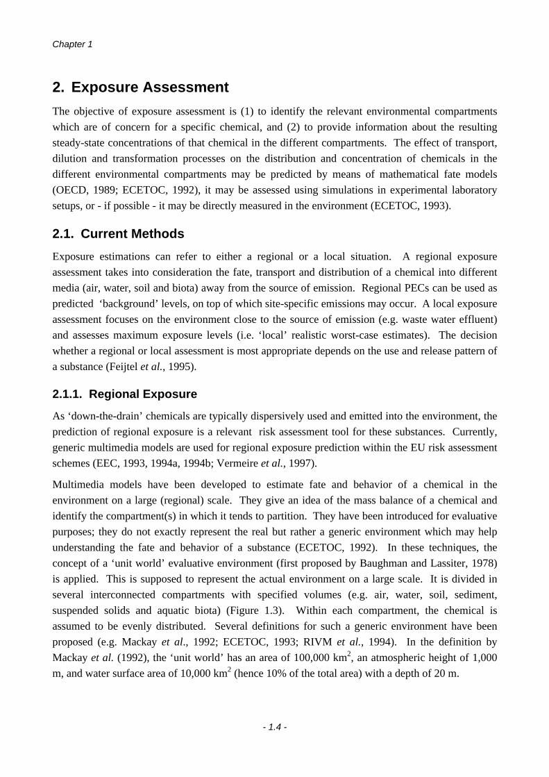
is applied. This is supposed to represent the actual environment on a large scale. It is divided in
several interconnected compartments with specified volumes (e.g. air, water, soil, sediment,
suspended solids and aquatic biota) (Figure 1.3). Within each compartment, the chemical is
assumed to be evenly distributed. Several definitions for such a generic environment have been
proposed (e.g. Mackay et al., 1992; ECETOC, 1993; RIVM et al., 1994). In the definition by
Mackay et al. (1992), the ‘unit world’ has an area of 100,000 km2, an atmospheric height of 1,000
m, and water surface area of 10,000 km2 (hence 10% of the total area) with a depth of 20 m.
Geo-referenced Environmental Risk Assessment, the GREAT-ER Project
- 1.5 -
transport
exchange
immission
Figure 1.3. Multimedia 'unit world' evaluative environment
Multimedia fugacity chemical fate models are used to predict the environmental partitioning or
removal of the chemical within the ‘unit world’, and its concentrations in the different
compartments (Mackay, 1991). Four classes of these models exist (Mackay and Paterson, 1981):
• Level I: equilibrium and steady-state are assumed, and transformation of the chemical is not
taken into account. Level I models help in identifying the ‘target’ compartments which may
have to be studied more extensively.
• Level II: equilibrium and steady-state are also assumed, but next to this chemical transformation
and advection are considered..
• Level III: since the rate of transfer between compartments is taken into account, not equilibrium
but only steady state is assumed. Level III models are built around a system of equations, one
for each compartment, which describe all inputs and outputs for each compartment. These
models present a more accurate estimate of chemical quantities and concentrations in each
environmental compartment, and of the chemical’s persistence.
• Level IV: non-equilibrium and non-steady state are assumed. Level IV models allow prediction
of the time required for the chemical to disappear from the environment once its use has ceased
or, alternatively, the time needed to reach steady-state when chemical releases are continuing.
These models use the same set of equations as Level III, but because of the non-steady state
assumption, solution becomes more complicated. The use of these models is only
recommended for estimating the disappearance of chemicals from the environment (ECETOC,
1992).

Chapter 1
- 1.6 -
The concept of fugacity, which drives these models, is well explained in Mackay & Paterson
(1981). Fugacity f can be regarded as the ‘escaping tendency’ of a chemical substance from a phase.
It has units of pressure (Pa). In the atmosphere, fugacity is usually equal to the partial pressure of a
substance. f can be related to concentrations C using a fugacity capacity constant Z, with units of
mol.m-3.Pa-1:
C Z f= ⋅ [1.1]
The fugacity capacity Z quantifies the capacity of the phase for fugacity. At a given fugacity, if Z is
low, C is also low, and only a small amount of substance is necessary to exert the escaping
tendency. Substances thus tend to accumulate in phases where Z is high, i.e. where high
concentrations can be reached without creating high fugacities. Z depends on temperature, pressure,
the nature of the substance, and the medium in which it is present. Its concentration dependence is
usually very limited at high dilutions (which is typical for environmental contaminants).
If there is contact between two phases, equilibrium of a substance will be reached when the
fugacities are equal. From this, it can be derived that the dimensionless partition coefficient
controlling the distribution of the substance between both phases is merely the ratio of their fugacity
capacities.
2.1.2. Local Exposure
Local air, water and soil models are designed to complement regional models, in order to refine the
prediction of actual substance concentrations for the compartment of concern, near the source of
emission. An overview of existing local fate and exposure models is given in ECETOC (1992).
Local models can be used to estimate maximum (initial) levels, and to quantify temporal and spatial
variations in concentrations at some distance from the emission, taking into account the relevant
fate processes (ECETOC, 1994b).
2.2. Limitations of Generic Regional Exposure Assessment Methods
Representing the environment in the form of ‘unit world’ models constitutes a large simplification.
An important drawback is that these models compute only one concentration value for each
compartment, whereas actual concentrations in the environment vary spatially and temporally
(Mackay & Paterson, 1981). Measurements indicate that this variation may range over several
orders of magnitude (ECETOC, 1988). Hence, these models are only suited to provide an
indication of concentrations in places far away from the source of emission. Therefore, their
quantitative results must be used with care (ECETOC, 1992).
Furthermore, in assessments using generic evaluative environments, regional averages or default
environmental characteristics are used, rather than geographically referenced specific information.
A typical example which is important for ‘down-the-drain’ consumer chemicals, is the connection
degree to domestic WWTPs. In the default European Union case (EEC, 1994b) a connection to

Geo-referenced Environmental Risk Assessment, the GREAT-ER Project
- 1.7 -
treatment of approximately 70% is put forward, hence leaving 30 % of the discharges untreated. As
spatial or temporal variability in environmental characteristics, river flows, degrees of treatment or
chemical emissions are not taken into account, the obtained results are not realistic, and are
therefore only applicable at screening level (European Science Foundation, 1995).
In Figure 1.4, it is illustrated how PECs are influenced by the connection degree to waste water
treatment and by chemical removal efficiency in such treatment. In this example, chemical removal
was varied between 80% and 99.9%, the WWTP connection degree was varied between 50% and
100%, the raw sewage chemical concentration was 1 mg/L, and dilution in receiving water was by a
factor 10 (assuming instantaneous and complete mixing). It is clear that with 70% waste water
treatment (cf. the generic EU case) PECs are much higher than under a situation with > 90%
connection. When an average treatment degree is used as the default for an entire region, the
resulting high PECs are used for risk assessment in areas where treatment is nearly complete as well
as areas where no treatment exists.
50%
60%
70%
80%
90%
100% 99.9%
99.0%95.0%
0
10
20
30
40
50
60 PEC(µg/L)
% Connection to treatment
% Removal in WWTP
Figure 1.4. PEC as a function of % treatment and removal efficiency
Previous and current legislation and industry strategies have stressed the importance of a high,
almost complete removal of consumer chemicals in WWTPs. In a situation where waste water
treatment is incomplete, the importance of this very high removal (> 99%) becomes less significant,
as even small percentages of directly discharged waste water cause high increases in environmental
concentrations. Thus, under these conditions efforts to develop readily biodegradable consumer
product ingredients are in part negated by the absence of adequate waste water treatment facilities.
Environmental risk and river quality will largely be affected by direct discharges, instead of treated
discharges of municipal treatment plants (Feijtel et al., 1997).

Chapter 1
- 1.8 -
It is obvious that the current generic exposure assessment approach causes two problems. For
chemicals which are highly removed in WWTPs, there is a large over-estimation of regional PECs
in the majority of EU waters, where treatment is adequate and wide-spread. This will lead to
environmental risk assessments which are too conservative. On the other hand, for so-called ‘hot
spots’, where no or limited treatment exists, the estimates of regional exposure are expected to be
too low. Risk assessments using these PECs can hence not be positioned in respect to the protection
goals and ecological quality objectives for the specific ecosystems.
A more detailed regional PEC calculation for geographies with a high connection to waste water
treatment should result in more realistic (and lower) PEC values, which correspond better to the
actual measured environmental concentrations. For the ‘hot spots’, a more detailed approach will
lead to the calculation of a realistic worst-case PEC, which will be significantly higher than the
'average' regional PEC. Present knowledge about the effects of direct untreated discharges of
individual chemicals on the freshwater environment is limited (e.g. Cowan & Masscheleyn, 1997).
Typically, no discrimination can be made between the effects of the chemical and of the untreated
sewage itself. It is therefore questionable whether the accepted chemical risk assessment procedures
can be applied with any confidence in these situations.
2.3. Geo-referenced Regional Exposure Assessment
Realism in regional exposure assessment can only be further introduced by verification of the
underlying assumptions of the applied fate models, and by taking into account the specific structure
and properties of the receiving environment as well as specific information on the waste water
treatment infrastructure (Feijtel et al., 1997). However, the use of specific, geo-referenced
information is fundamentally in conflict with the concept of a generic evaluative environment.
Hence, a geographically referenced regional exposure assessment methodology is required to
improve regional PEC estimation compared to the current generic approach.
2.3.1. Geo-referenced Evaluative Environments
For several regions, the ‘unit world’ concept has been applied in a geo-referenced way. In this
approach, large geographical entities (such as countries) are divided into smaller regions, for which
the generic environmental parameters are replaced by specific data. Examples are France
(CHEMFRANCE: Devillers et al., 1995), Canada (CHEMCAN, applied in e.g. Mackay et al.,
1996), and Denmark (Severinsen et al., 1996). Although the accuracy of these region-specific
applications of the ‘unit world’ concept is generally higher compared to the generic methods, they
still have to deal with the same fundamental drawbacks as the latter.

Geo-referenced Environmental Risk Assessment, the GREAT-ER Project
- 1.9 -
2.3.2. Regionalizing of Local Exposure Assessment
Another method of including a geographical aspect in regional exposure assessment, is to develop a
regional exposure prediction by means of local exposure models. To achieve this, a region is to be
split up into a large number of interconnected ‘local’ environments, for all of which local PECs are
to be calculated. In the ROUT model (Rapaport and Caprara, 1988), information about the location
and emissions of individual WWTPs is combined with data on river flows. As this model is linked
with several pan-USA databases, geo-referenced chemical fate simulations are possible which result
in aquatic PECs for all main rivers in the USA (Caprara and Rapaport, 1991). The ROUT approach
has also been applied to the river Rhine (Hennes and Rapaport, 1989). In the US-EPA water quality
assessment model BASINS (Whittemore, 1998), a simple river dilution and fate model for
performing screening-level assessments of toxic pollutants (TOXIROUTE) was combined with a
GIS (Geographical Information System), to allow visualization of geo-referenced predicted
exposure in rivers. A simplified simulation of individual chemical fate is also possible in the GIS-
based water quality model NOPOLU (Béture-Cérec, France).

Chapter 1
- 1.10 -
3. The GREAT-ER Project
The work described in this thesis (see section 4 of this chapter) was mainly conducted in the
framework of the GREAT-ER project. To situate this work, a description of the entire project is
given in this section.
The GREAT-ER project (Geography-referenced Regional Exposure Assessment Tool for European
Rivers) (Feijtel et al., 1997; Matthies et al., 1997; Boeije & Schowanek, 1997) aims to refine PEC
calculations of ‘down-the-drain’ consumer chemicals in the aquatic environment. A new fate
simulation concept was developed to obtain more reliable predictions, which are to be applicable at
a higher risk assessment tier than the current methods. Geo-referenced ‘real’ datasets are applied
instead of generic or average values. To account for temporal variability and uncertainty, PECs
were defined as statistical distributions. Predicted concentrations can be visualized and (spatially)
analyzed by means of a Geographic Information System (GIS).
Compared to the existing GIS-linked chemical fate models (see higher, 2.3.2), GREAT-ER is more
advanced. It is specifically dedicated to chemical fate simulation and allows the use of more
complex and detailed fate models. Its built-in analysis tools are focused on environmental exposure
assessment and PEC calculations. Finally, it allows to perform uncertainty and variability analyses.
3.1. Modular Approach
The project was approached in a modular way (Figure 1.5):
• Geographical Data Methodology - input data sourced from several data bases (and from the
hydrology module) were transformed into appropriate GIS formats, including geographical
segmentation
(work performed by the Institute of Environmental Systems Research, University of Osnabrück,
Germany)
• Hydrology - several hydrological databases were combined with a hydrological model, to provide
the GREAT-ER system with the required flow distributions and river characteristics
(work performed by the NERC Institute of Hydrology, Wallingford, UK)
• Chemical Fate Modeling - prediction of chemical emission, of transformations during
conveyance and treatment, and of chemical fate in rivers, resulting in geo-referenced frequency
distributions of predicted concentrations
(work described in this thesis)

Geo-referenced Environmental Risk Assessment, the GREAT-ER Project
- 1.11 -
• GIS / Model Integration - access to and visualization of the data banks and model results was
achieved, as well as the linking of the models with the data banks
(work performed jointly with the Institute of Environmental Systems Research, University of
Osnabrück, Germany)
• Monitoring - to provide the specific environmental measurements required for model calibration
and corroboration
(work performed by a task force of the European Center for Toxicology and Ecotoxicology of
Chemicals - ECETOC, the UK Environment Agency, and the University of Milan, Italy)
Chemical Emission +Waste Water Pathway Data Hydrological Data
Hydrological Model
Hydrological Data Collation
MONITORING
Waste WaterPathway Model
RiverModel
Waste WaterPathway Data
Main RiversData
ChemicalMarket Data
OUTPUTdesktopGIS
GIS Data Processing
full GIS
Figure 1.5. GREAT-ER project: modular approach
3.2. Geographical Data Methodology
3.2.1. Scope and Scale
A blueprint system (‘prototype’) was developed, and applied to 2 main pilot study areas: in northern
Europe: UK, Yorkshire Ouse (15,000 km2), and in southern Europe: Italy, Lambro (sub-catchment
of the Po, near Milan) (1,000 km2). Next to this, GREAT-ER was also applied to the Itter, Rur and

Chapter 1
- 1.12 -
Untermain (Germany), and the Rupel (Belgium). The ultimate objective is to implement the
GREAT-ER system for the entire European Union.
The blueprint system is scale-independent. The scale is only determined by the scale of the used
geographically-referenced data bases. Hence, one specific area can be modeled at a small detailed
scale or at a large, less detailed scale. Based on the pilot study area experiments, an optimal range
of geographical scales for the pan-European application will have to be determined. Typically, such
an optimal scale will represent a compromise between data availability, model complexity and
desired accuracy.
3.2.2. Geographic Information System (GIS) Data Processing
A GIS approach was used for data storage and visualization. This allows an easy data access by the
fate models, and user-friendly interactions. Moreover, it allows spatial analysis and interpretation of
model results. A flexible, data-driven approach is followed. The general data structure is based on
digital river networks. Both river properties and information on waste water discharges (and
emission) are related to river stretches, which are geo-referenced within a network.
For the transformation of various input data sources, specific GIS data conversions and
transformations were to be applied (Wagner & Matthies, 1997). The software ARC/INFO (ESRI,
Redlands, Ca., USA) was used for this purpose. Geographical segmentation was also performed
using this tool.
3.3. Hydrology
3.3.1. Digital River Network and Hydrological Data
Pan-European river network data can be sourced from the CORINE large scale digital rivers. For
the UK pilot study area, the required information was obtained from the Micro Low Flows
( NERC-Institute of Hydrology, Wallingford, UK) database. For the Lambro, detailed river
networks were digitized from base maps. Flow distribution curves were derived from time-series
flow measurements. These are characterized by their mean and 5th percentile (defined as Q95, the
flow which is exceeded in 95% of time). The measured flow information was entered into the
geographically referenced hydrological data bank. The principal source of measured pan-European
flow data will be the European FRIEND databases, the EEC CORINE river flow database, and the
GRDC (Global Runoff Data Center).
3.3.2. Hydrological Modeling
For ungauged river stretches, hydrological model results were used to complement flow data in the
hydrological data bank. There is a considerable variation in the behavior of river flows across
Europe, depending on climate, physical catchment properties, and artificial influences. A
quantitative hydrological model, based on existing methods (Gustard et al., 1992) was used for flow

Geo-referenced Environmental Risk Assessment, the GREAT-ER Project
- 1.13 -
predictions. These methods were adapted to incorporate seasonality of low flows, local hydrometric
data, and different hydrological situations.
In general, a step-wise approach was applied: (1) the average annual runoff and a local estimate of
mean flow were calculated from a simple water balance model, where the catchment average values
were estimated from maps; (2) the flow distribution curve was derived: characterization of the
catchment low flow response by a multivariate regression model, derivation of a dimensionless flow
duration type curve characteristic for such low flow response, and re-scaling of the selected curve by
the local estimate of mean flow.
Flow velocities were derived from a statistical relation with flow characteristics (Round et al.,1998). Velocities are required for the calculation of the hydraulic residence time in a river stretch,
and hence for the estimation of in-stream-removal of chemicals.
3.4. Chemical Fate Modeling
3.4.1. Deterministic Models
Mechanistic chemical fate models were applied (Boeije et al., 1997). These describe the behavior /
removal of chemicals in the main compartments of the technosphere and the ecosystem. A
distinction was made between chemical sorption, volatilization, biological degradation, non-
biological degradation, etc. The fate kinetics for these different processes were estimated from
physical / chemical and biological properties of the considered substances, and from relevant
environmental parameters.
The chemical fate model consists of two main sections: (1) a waste water pathway model, used to
estimate the emission of chemicals, their transport and fate through the waste water conveyance
system, and their removal in treatment plants (e.g. Struijs, 1996); and (2) a river fate model, which
is used to calculate PECs along ‘main’ rivers (e.g. Trapp & Matthies, 1996).
3.4.2. Stochastic Aspects
By means of Monte Carlo simulation, a stochastic layer was added on top of the deterministic fate
simulation core (e.g. NRA, 1990). This deals with the inherent variability of the environment
(seasonality: flow distributions, temperature, wind speed,...) and parameter uncertainty (e.g.
uncertainty on chemical consumption, on physical/chemical properties,...). Variability and
uncertainty may be captured in statistical frequency distributions. In each Monte Carlo ‘shot’,
discrete samples are taken from these distributions, and used as input for the deterministic fate
models. This hybrid approach finally results in statistical distributions of predicted concentrations
for each river stretch.

Chapter 1
- 1.14 -
3.5. GIS / Model Integration
The (standardized) GIS data banks and the chemical fate models were integrated into one coherent
simulation system (Wagner & Matthies, 1997). Statistical and spatial analysis tools can also be
integrated. Data transfer between the GIS and the models can be performed by means of direct or
indirect coupling. In the latter approach, a GIS / Model Interchange Server (GMIS) is used to
generate the appropriate model input data formats from the data banks, and to convert simulation
results back to a GIS format (Figure 1.6).
Figure 1.6. GREAT-ER project: GIS / model integration methodology
For the end-user software, the desktop GIS ArcView version 3.0a (ESRI, Redlands, Ca., USA) was
applied. From this easy-to-use front end, simulations can be launched, input data can be reviewed,
and results can be visualized and interpreted (Wagner & Matthies, 1997).
HYDROLOGICALMODEL
Spatial Data Processing (ARC/INFO GIS OPERATION)
SCENARIOS,DISTRIBUTIONS
Standardized Geo-referenced Database (coverages and attributes) Arc/Info data format
Catchment Properties, Demography, Chemical Data, Runoff, River Network, Hydrology, Water Quality
WASTE WATERPATHWAY MODELS RIVER MODELS
Waste Water Pathway Fate and Quality, River Fate and Quality
ANALYSISTOOLS
STATISTICSSENSITIVITYUNCERTAINTY
GIS-MODEL INTERCHANGE SERVER (GMIS)
User Input
end-user simulation tool (ArcView / models)
Calculation & Visualization of PECs
ChemicalProperties
ChemicalMarket Data
Environmental, Demographical and Technological Information

Geo-referenced Environmental Risk Assessment, the GREAT-ER Project
- 1.15 -
3.6. Monitoring - Calibration and Verification
3.6.1. Monitoring Program
Linear Alkylbenzene Sulphonate (LAS) and Boron (B) were used as test chemicals. LAS is a
biodegradable surfactant used in consumer detergents, which mainly enters the environment via
domestic waste water discharges. The majority of Boron in the freshwater aquatic environment is
coming from detergents. Since B is chemically inert and water soluble, this chemical can be used as
a convenient tracer. For both analyses, well validated analytical methodologies are available.
Particular attention was given to ensure that samples taken for LAS determinations were adequately
preserved and stored prior to analysis.
Frequency distributions (time series) of environmental concentrations were measured at several
locations in the British and Italian pilot study areas (Holt et al., 1997). Additional studies were
performed to analyze the fate of the test chemicals in trickling filter sewage treatment works (Holt etal., 1998). LAS removals during activated sludge waste water treatment have been reported
elsewhere (e.g. Waters & Feijtel, 1995; Holt et al., 1995). Experiments to determine the in-stream
removal of these chemicals in rivers were also conducted (Fox et al., submitted).
3.6.2. Calibration and Verification
Concentrations in water were calculated using the developed simulation system, and were compared
to measured values. Initially, monitoring results were used to calibrate and fine-tune the modeling,
to improve the predictive power. Finally, they served to test the reliability of the predictions. An
initial target accuracy factor of less than 5 was aimed for within the scope of geographical exposure
and risk assessment (Feijtel et al., 1997). This desired accuracy factor should be positioned against
the much lower accuracy obtained with the generic multimedia models (of which the predictions
may differ from monitoring data by several orders of magnitude), and also against the high
variability which is encountered in the environment.
3.7. Summary
The output of GREAT-ER is a distribution of geo-referenced predicted concentrations, on a regional
level, including seasonality and / or uncertainty. The chemical-specific input data for the model are
the physical/chemical and biochemical parameters, together with geographical consumption patterns
or market data. Required environmental information was taken from available geography-linked
databases. For the storage and the access of the majority of these data in a user-friendly format, and
for results visualization and analysis, a Geographic Information System (GIS) was used.
The final deliverable of this project is a software prototype of the exposure assessment tool. This
prototype is applicable globally, and was calibrated and validated for a number of pilot study areas.
The resulting PC software was made freely available (under license agreement).

Chapter 1
- 1.16 -
4. Overview of this Thesis
The work described in this thesis was mainly conducted in the frame of the GREAT-ER project. A
geo-referenced exposure simulation methodology was developed and implemented in an appropriate
software system, which could be linked with the GIS user interface and data base. Chemical fate
models of different complexity levels were selected, and if necessary adapted or newly developed.
In this thesis, only novel aspects are dealt with; for a complete description of the model selection,
reference is made to the GREAT-ER user manual and technical documentation (ECETOC, 1999).
Finally, to increase the practical applicability of geo-referenced exposure assessment, a technique to
obtain spatially aggregated PECs was worked out and tested.
This thesis can be split up into three main sections: (1) methodology; (2) measurement and
prediction of chemical fate; and (3) analysis (Figure 1.7). The methodology and analysis sections
are at the highest ‘hierarchical level’, and are an integral part of the GREAT-ER concept. Section
(2), on the other hand, is situated at the more detailed level of individual chemical fate processes.
• development of methodology (2)• hypothetical case study (3)
METHODOLOGY
• PEC calculation (10)
ANALYSIS
• Waste water treatment - activated sludge with nutrient removal (4, 5) - trickling filter (6, 7)• Rivers (8)• Sewers (9)
MEASUREMENT + PREDICTION OF CHEMICAL FATE
GREAT-ER
detailed chemicalfate analysis
Figure 1.7. Overview of this thesis (chapter numbers between brackets)
Methodology
A new exposure assessment methodology was worked out and implemented. The development of a
geo-referenced aquatic exposure prediction methodology for ‘down-the-drain’ chemicals is
presented in chapter 2. Steady-state deterministic chemical fate models were combined with a
Monte Carlo simulation to obtain statistical frequency distributions of predicted concentrations in
the aquatic environment. Issues related to uncertainty and variability are only briefly discussed, as a
complete uncertainty analysis was outside the scope of this thesis. The new simulation approach
was tested by means of a hypothetical (but realistic) case study, which illustrated its practical
applicability and independence of scale (chapter 3).
Geo-referenced Environmental Risk Assessment, the GREAT-ER Project
- 1.17 -
Measurement and Prediction of Chemical Fate
This section deals with measuring and modeling environmental fate of ‘down-the-drain’ chemicals
in the three main steps of their aquatic fate pathway: sewers, waste water treatment plants and
rivers. Measurements were only conducted for the surfactant LAS, as this was the GREAT-ER
project’s main test substance. Although the presented fate models are in principle applicable to any
chemical they could only be tested for LAS. Hence, to examine their validity for other substances
(e.g. volatile compounds) additional research will be required.
The new developments in environmental fate modeling reported in this thesis mainly focus on the
use of site-specific information rather than generic parameters (such as ‘typical’ waste water
treatment plants or ‘typical’ rivers). This way, it was attempted to increase the realism of the
exposure predictions. The new or adapted fate models can find their application in geo-referenced
exposure assessment in general, and in GREAT-ER in particular. However, the presented models
may also be useful to increase the realism of non-geo-referenced exposure evaluations using generic
evaluative environments.
The standardized Continuous Activated Sludge (CAS) laboratory test system (OECD, 1993) and the
mathematical fate model SimpleTreat (Struijs, 1996) are used to routinely assess the elimination of
substances in activated sludge waste water treatment plants. The effects of biological nutrient
removal processes (BNR) on chemical fate are not included in the CAS test nor in SimpleTreat. As
BNR is rapidly gaining importance in waste water treatment practice, a number of modifications
were worked out. The adaptation of the CAS test to include BNR processes is described in chapter
4. The performance of two modified test units, which were fed with an improved synthetic sewage
(developed as part of this study), was monitored and compared with model simulations. Similarly,
the SimpleTreat model was modified to increase its applicability to BNR plants (chapter 5). The
adaptations focused on an improved description of sludge recycling and on the presence of different
redox zones in the biological reactor. Two updated models were applied to the bench-scale
WWTPs developed in chapter 4, and confronted with measurements of LAS removal in these
systems.
The development and operation of a pilot-scale high-rate trickling filter waste water treatment plant
and removal measurements of LAS in this system are presented in chapter 6. As for trickling filters
no standardized chemical fate model existed, a new fate model was developed based on the steady-
state non-equilibrium approach used in SimpleTreat in combination with an existing biofilm model
(chapter 7). To test this model, it was applied to predict the fate of LAS in the lab-scale test unit,
and to two full-scale domestic trickling filters in Yorkshire (UK), for which LAS removal had been
monitored within the GREAT-ER project (Holt et al., 1998).

Chapter 1
- 1.18 -
In chapter 8, modeling chemical fate in rivers was worked out, supported by artificial river
experiments. To predict the in-stream biodegradation, a mathematical model was developed which
considers both biofilm and suspended biomass activity. To calibrate this model for LAS,
experimental data were obtained in a small lab-scale artificial river system. The model was further
tested by comparing its predictions to a detailed field study in the Red Beck, a small Yorkshire river
(Fox et al., submitted).
A tentative fate measurement of biodegradable surfactants in the sewer system is presented in
chapter 9.
Analysis - calculation of Predicted Environmental Concentrations (PEC)
The direct results of GREAT-ER simulations are digital maps with predicted concentrations for
individual river stretches. As this output may contain too much local detail for practical risk
assessment applications and decision making, a spatial aggregation is desirable. In chapter 10, the
development of new PECs based on the spatial aggregation of local predicted concentrations is
discussed, as well as issues related to scale-dependency and stretch selection. Tests for 2 pilot study
catchments (Calder and Went, Yorkshire, UK) are also presented in this chapter.

Chapter 2 -
A Geo-referenced Aquatic Exposure PredictionMethodology for ‘Down-the-Drain’ Chemicals
a condensed version of this chapter was published as:
Boeije, G., Vanrolleghem, P. & Matthies, M. (1997). A geo-referenced aquatic exposure predictionmethodology for 'down-the-drain' chemicals (Contribution to GREAT-ER #3). Water Science and
Technology, 36(5), 251-258.

- 2.1 -
Chapter 2
A Geo-referenced Aquatic Exposure PredictionMethodology for ‘Down-the-Drain’ Chemicals
A geo-referenced simulation methodology for the prediction of aquatic exposure to individual
‘down-the-drain’ chemicals (consumer chemicals which mainly enter the environment via the
domestic waste water route, e.g., detergents) was developed. This method uses real-world data,
including their spatial and temporal variability. It results in statistical frequency distributions of
predicted concentrations in the aquatic environment. A stochastic / deterministic simulation
approach is used. Steady-state deterministic models, which describe chemical fate, form the
system’s core. A stochastic (Monte Carlo) simulation is applied on top of this. From chemical
market data, combined with information on the location of consumers and their emission habits,
geo-referenced domestic chemical emissions are predicted. These emissions are further processed
in sewer and treatment models, to obtain predicted chemical fluxes to rivers. The emission fluxes
are entered into a river model, resulting in (geo-referenced) predictions of chemical concentrations
in the considered river systems.
1. General Simulation Approach
To deal with statistically distributed inputs and outputs, a hybrid simulation approach is used,
involving both stochastic and deterministic techniques. The model core is deterministic. By means
of Monte Carlo simulation, a stochastic layer is added on top of this core. A large number of
‘shots’, which are discrete samples from the distributed data set, are generated. For each distributed
input parameter, there exists a discrete counterpart in the ‘shot’, which was sampled at random from
the input distribution. For each of these ‘shots’, the deterministic model is called, which contains a
mechanistic description of the considered processes in the rivers and in the waste water drainage
areas. Process rates are derived from knowledge about chemical properties and process specifics.
Finally, the (discrete) results from each ‘shot’ are statistically analyzed, to obtain distributed results
as simulation output.
For reasons of model and data set simplicity and computation performance, only steady-state model
formulations are applied. Hence, a number of fundamental assumptions are made: (1) constant
chemical emissions: diurnal patterns in product and water consumption are disregarded, as well as
variations between different days of the week; (2) constant flows within each steady-state model
calculation run; (3) constant environmental properties.

Chapter 2
- 2.2 -
To allow a straightforward mass-balancing approach, all determinands (chemical levels, water
flows) are expressed as fluxes. Chemical mass fluxes Φ (mass/time) are applied to describe
chemical loads. Water flows are expressed as volumetric fluxes Q (volume/time). In the models,
chemical concentrations C (mass/volume) are not used, because they are not independent of water
flows, and they do not describe chemical transport. Chemical mass fluxes, on the other hand, are
independent of dilution or flow (unless this dependency is implicitly included in the models which
are used to calculate chemical mass fluxes). When concentrations are explicitly required, they are
derived from the chemical mass fluxes and the hydrological volumetric fluxes: C = Φ / Q.
Simulations can be performed for different scenarios (i.e., evaluations of different chemicals and
chemical consumption patterns). The simulation input consists of a scenario-independent and a
scenario-dependent data set. These data are expressed as statistical frequency distributions,
incorporating seasonality and parameter uncertainty. Environmental characteristics are constant,
and hence non-scenario-dependent. These include the river network structure, flow and flow
velocity distributions, discharge point locations, treatment plant information, emission data,
properties of sewers and small surface waters, etc. Chemical-specific information is scenario-
dependent: chemical properties (i.e., biological, chemical and physical properties, specific process
rates,...), and chemical market data (i.e., per capita product consumption rates). Market data are
geo-referenced in the same way as the waste water information (i.e., related to waste water
discharge points).
The simulation input data are expressed as statistical frequency distributions. This allows to include
both seasonality effects and parameter variability and/or uncertainty into the simulation input. For
river flows and flow velocities, the lognormal distribution is used (after NRA, 1995). For
hydrological information this distribution is described by the mean and the 5th percentile. In the
case of flows, there is a 95% probability that the 5th percentile low flow (also referred to as Q95) is
exceeded: P(Q>Q95) = 0.95.
The simulation results are frequency distributions of chemical concentrations, incorporating
temporal variability. For risk assessment purposes, these can be expressed as lognormal
distributions, defined by their mean and 95th percentile values. Predicted concentrations are geo-
referenced in the same way as the input data set: river concentrations are associated with a river
network structure, and waste water drainage area concentrations are associated with discharge
points. Within one location, a further differentiation is made between the maximal predicted
concentrations (i.e., upon discharge), the minimal predicted concentrations (i.e., after degradation
processes), and an ‘internal’ average value. For the calculation of the latter, specific algorithms
have to be provided in the deterministic models.
A Geo-referenced Aquatic Exposure Prediction Methodology for ‘Down-the-Drain’ Chemicals
- 2.3 -
2. Segmentation
2.1. General
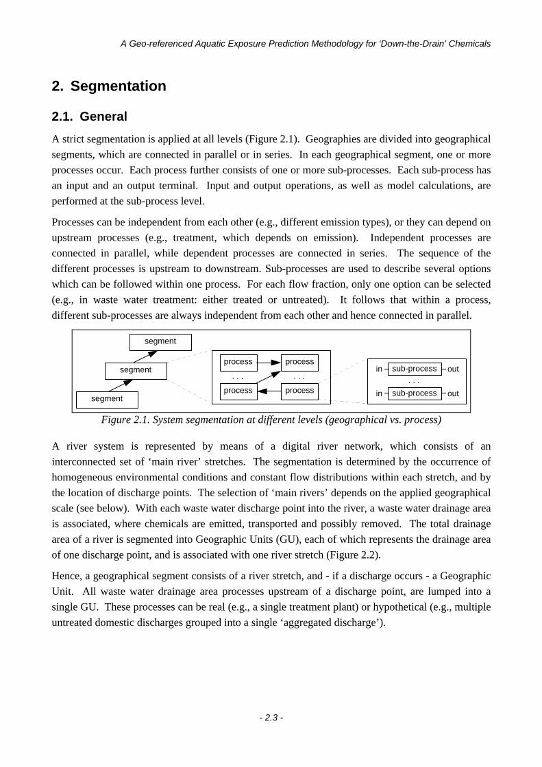
A strict segmentation is applied at all levels (Figure 2.1). Geographies are divided into geographical
segments, which are connected in parallel or in series. In each geographical segment, one or more
processes occur. Each process further consists of one or more sub-processes. Each sub-process has
an input and an output terminal. Input and output operations, as well as model calculations, are
performed at the sub-process level.
Processes can be independent from each other (e.g., different emission types), or they can depend on
upstream processes (e.g., treatment, which depends on emission). Independent processes are
connected in parallel, while dependent processes are connected in series. The sequence of the
different processes is upstream to downstream. Sub-processes are used to describe several options
which can be followed within one process. For each flow fraction, only one option can be selected
(e.g., in waste water treatment: either treated or untreated). It follows that within a process,
different sub-processes are always independent from each other and hence connected in parallel.
segment
segment. . .
process
process
process
. . .
process
. . .
segment
sub-processin out
sub-processin out
Figure 2.1. System segmentation at different levels (geographical vs. process)
A river system is represented by means of a digital river network, which consists of an
interconnected set of ‘main river’ stretches. The segmentation is determined by the occurrence of
homogeneous environmental conditions and constant flow distributions within each stretch, and by
the location of discharge points. The selection of ‘main rivers’ depends on the applied geographical
scale (see below). With each waste water discharge point into the river, a waste water drainage area
is associated, where chemicals are emitted, transported and possibly removed. The total drainage
area of a river is segmented into Geographic Units (GU), each of which represents the drainage area
of one discharge point, and is associated with one river stretch (Figure 2.2).
Hence, a geographical segment consists of a river stretch, and - if a discharge occurs - a Geographic
Unit. All waste water drainage area processes upstream of a discharge point, are lumped into a
single GU. These processes can be real (e.g., a single treatment plant) or hypothetical (e.g., multiple
untreated domestic discharges grouped into a single ‘aggregated discharge’).

Chapter 2
- 2.4 -
Reality Model
river stretchGU
river stretch
river stretchGU
river stretchGU segment
segment
segment
segment
Figure 2.2. Geographical segmentation methodology used in GREAT-ER
The modeling and simulation methodologies, as well as the GIS data methodology, are scale-
independent. In the upscaling process (i.e., moving from a smaller, detailed scale to a larger, less
detailed scale), multiple discharge points can be aggregated into single (hypothetical) discharges;
several smaller rivers are no longer considered as ‘main rivers’, but are transferred to the waste
water discharge model and aggregated into a single (hypothetical) ‘small surface water’. In the
large scale approach, the mouth of a small rivers’ catchment into a large river is represented by a
discharge point. Hence, for different scales, only the geo-referenced data set is different; the applied
models are identical. In Figure 2.3, a system is modeled at a small (left) and at a large scale (right).
In this example, a complex system of ‘main rivers’ is used for the small scale, each with individual
waste water discharges. In the large scale approach, the system is reduced to a single ‘main river’
with a single discharge point.
RealitySmall Scale Large Scale
GUGU
GU
GU
GU
GU
GU
GU
Figure 2.3. Geographical scale flexibility (illustration)
2.2. Geographical Database Structure
A set of five separate databases are used to store all required geo-referenced information:
• a river database, in which river stretch specific information is stored (e.g., flow and flow
velocity)
• a waste water pathway (discharge) database, which contains information about the GUs
(population, sewer network) and links to the information about treatment infrastructure,

A Geo-referenced Aquatic Exposure Prediction Methodology for ‘Down-the-Drain’ Chemicals
- 2.5 -
• a river class database, which contains data that are specific for groups of rivers, but not for
individual stretches,
• a WWTP database, in which treatment plant specific data are stored, and
• an emissions database, with information about market data and non-domestic emissions.
The river network segmentation is the ‘backbone’ of the geographical data structure. Each river
stretch which receives waste water is directly related to its GU, as the same identification code is
used for both. Each river stretch belongs to one specific river class, of which the identification code
is known in the river database. Each waste water discharge segment is associated with an emission
data point. If a GU contains a WWTP, then there is a link to the WWTP database.
The following example clarifies this data structure concept. The catchment shown in Figure 2.4
consists of two rivers: a main river, divided into 6 segments, and a tributary, divided into 2
segments. There are 3 waste water discharge points: a large city (AS waste water treatment,
segment 5), a first small city (TF waste water treatment, segment 3), and a second small city (TF
waste water treatment, segment 8). Suppose that several river classes have been defined, and that
the main river (segments 1..6) belongs to river class 1, and the tributary (segments 7..8) to another
river class 3. Assume that we have exact information on the activated sludge plant (AS) in segment
5, but no exact information on both trickling filter (TF) plants. Further, assume that chemical
market data for the entire catchment belongs to the emission category 2. The associated data
structure, with the links between the different databases, is shown below in Figure 2.5.
TF
1
2
3
4
5
6
AS
TF
5
8
3
7
8
Figure 2.4. Data structure example (catchment)

Chapter 2
- 2.6 -
• seg 1• seg 2• seg 3• seg 4• seg 5• seg 6• seg 7• seg 8• ...
real:• wwtp 1• wwtp 2•...
default:• AS• AS + NR• TF • ...
• seg 3
• seg 5
• seg 8•...
• rc 1• rc 2• rc 3•...
RIVERCLASS
RIVER DISCHARGE
WWTP
• emission 1• emission 2• ...
EMISSIONCORE
Figure 2.5. Data structure example
3. Deterministic Model
In environmental exposure assessment, several applications are related to ‘new’ chemicals, of which
the safe use is to be assessed. Since these chemicals are generally still in a development phase, or
have not been marketed yet, environmental concentration measurements, which are required for
statistical modeling (e.g., Helsel and Hirsch, 1992), can not be obtained. Hence, knowledge-derived
deterministic models need to be applied. In such models, the chemical, physico-chemical and
biological properties of a substance are combined with the properties of the receiving environment
and with information about emissions, to predict the environmental fate and distribution of the
substance (Feijtel et al., 1995).
In the deterministic model, all geographical segments are sequentially simulated (upstream to
downstream). For each segment, the influent (from upstream segments) is calculated; if required
the waste water pathway simulation is performed; the ‘main river’ processes are simulated; and
finally the effluent (flowing to downstream segments) is calculated.

A Geo-referenced Aquatic Exposure Prediction Methodology for ‘Down-the-Drain’ Chemicals
- 2.7 -
3.1. Segment Selection
A recursive tree-walking algorithm is used to find the correct segment sequence. The algorithm
climbs up into the river network from the most downstream segment (i.e., the root of the tree), until
the most upstream segments (i.e., the leaves of the tree) are detected. At confluences, both upstream
directions are climbed, one after the other. At bifurcations, the upstream climbing is ended if the
upstream part has already been climbed before, i.e., when coming from the other side of the
bifurcation. Next, the network is again descended. Each segment which is encountered during the
descent is selected and simulated. This way, influent data (from upstream) are always available to
downstream segments. An example of the selection methodology is shown in Figure 2.6 (the
numbers indicate the sequence in which the segments are called for simulation).
end of tree 1
2
end of tree3
4
5
confluence 6
confluence9
bifurcation7
8
(root)10
bifurcation
Figure 2.6. Sequential segment selection
3.2. Influent and Effluent Calculation
Segment influents and effluents are discrete values, as they are only required within each ‘shot’.
For the influent, only chemical fluxes are calculated. Each segment’s influent flow is set to the
segment’s ‘main river’ flow, which is taken as such from the (hydraulically consistent) geo-
referenced data set. In the ‘normal’ case (with only one upstream segment), a segment’s influent
chemical mass flux is set to the upstream segment’s effluent. At a confluence, complete and
instantaneous mixing is assumed, hence the influent is equal to the sum of the upstream effluents.
At a bifurcation, the upstream segment’s effluent is split into two fractions, proportional to the
(known) river flows in each stretch downstream of the bifurcation. The effluent of a segment is
identical to the effluent of the segment’s ‘main river’ stretch. Hence, no effluent calculations are to
be performed as such.

Chapter 2
- 2.8 -
3.3. Individual Process Modeling Concept
3.3.1. General
Each process model exists at two levels: at the detailed process rate calculation level, and at the
conceptual segment level. At the detailed level, different models can be used in different software
implementations. At the conceptual level, described in this chapter, the model format is
implementation-independent. Models are considered as ‘open boxes’, each of which applies to one
sub-process. The general model expression for one determinand within each sub-process is:
x a x bout in= ⋅ + [2.1]
with a chemical conversion factorb emission valuexin sub-process input valuexout sub-process output value
Emissions and conversion factors are obtained at the detailed model level. At this level, several
model formulations (e.g., Monod or first-order kinetics describing biodegradation) and solution
algorithms (e.g., analytical or numerical) can be applied. Emission models are described by one
emission value for each determinand. Their output is this set of emission values. Obviously, no
input is required. Chemical fate is simulated by means of transport / conversion models. These are
described by the chemical removal fraction R, which is calculated at the detailed model level. A
ground water leakage fraction L can also be applied. L is part of the sub-process outflow
fractionation, taken as such from the geo-referenced data set. The input vector of a transport /
conversion model, as well as the output vector, is a set containing a value for each simulated
determinand.
3.3.2. Waste Water Pathway Model
The waste water pathway model is used to predict the properties of discharges into ‘main river’
stretches. It consists of both emission and transport / conversion processes. A (simplified)
overview of what is meant with the ‘waste water pathway’ concept is given below in Figure 2.7.
The waste water pathway model focuses on the fate of ‘down-the-drain’ chemicals. These
consumer chemicals are (mainly) emitted via the domestic sewage pathway. After use in the
households, they are flushed down the washing machine’s drain, the kitchen sink, the bathroom
drain, or the toilet. Next to these domestic emissions, industrial and / or agricultural emissions may
occur in exceptional, site-specific and chemical-specific cases. Emission to water by land runoff is
very unlikely.

A Geo-referenced Aquatic Exposure Prediction Methodology for ‘Down-the-Drain’ Chemicals
- 2.9 -
WWTP
UntreatedDischarge
Treated Discharge
Disperse UntreatedDischarges
Sewers
On-siteTreatment
Bypass
Untreated Discharge
Figure 2.7. Waste water pathway of ‘down-the-drain’ chemicals (illustration)
Three types of chemical emission into the waste water pathway are considered:
- domestic emission (blackwater, i.e., chemicals together with sanitary waste; and greywater, i.e.,
chemicals discharged separately);
- non-domestic emission (industrial and agricultural); and
- land runoff.
Five transport / conversion processes are considered along the pathway:
- domestic on-site treatment (e.g., septic tanks);
- sewers (combined sewers or separate sewers);
- waste water treatment;
- ground water leakage; and
- small surface waters.
Process interconnection
The outflow of each sub-process is split into a number of fractions, each of which is connected to
one downstream sub-process. One or more downstream steps can be ‘skipped’, e.g., a domestic
emission outflow fraction can be connected directly to the ‘main river’ discharge point. Emission
processes are always at the most upstream level - they do not receive any inflow. The sequence of
the transport / conversion processes is: on-site treatment → sewer → treatment plant → ground
water → surface water. The architecture of the interconnection between processes is identical for
each segment. The (simplified) interconnection for domestic waste water pathway processes is
shown in Figure 2.8.

Chapter 2
- 2.10 -
DomesticEmission
black-water
grey-water
On-siteTreatment
none
septictank
Sewer
sepa-rate
com-bined
un-treated
treated
TreatmentPlant
GroundWater
SmallSurfaceWater
River
Figure 2.8. Domestic waste water pathway process interconnection within a segment (simplified)
3.3.3. River Model
The river model is used for the ‘main river’ process in all segments. The model’s inflow is the sum
of the segment influent (from upstream segments) and the segment’s waste water discharge (if
applicable). The river model is a transport / conversion model, without leakage step. Water flows
are not simulated but are taken as such from the geo-referenced data set. Hence, the process is
completely determined by the chemical removal fraction, which is obtained at the detailed model
level (e.g., Cowan et al., 1993a; Trapp & Matthies, 1996).
3.4. Calculation Approach
For each determinand (i.e., flow, chemical flux, etc.), the system of steady-state model equations for
an entire segment consists of one equation [2.1] for each sub-process. The system can be expressed
as:
X A X Bi i i i= ⋅ + [2.2]
with:
Ai (square) transport/conversion matrix for determinand i, with elements aik,l
Bi emission vector for determinand i, with elements bik
Xi state variables vector for determinand i, with elements xik
The vectors Xi and Bi are partitioned per process, within a process per terminal, and finally within a
terminal per sub-process (e.g. sewer - outputs - combined sewer). The process sequence in the
arrays is from upstream to downstream; the terminal sequence is first input, then output. Hence,
determinand values at a specific situation are only dependent of values at more ‘upstream’
situations. Consequently Ai is a lower triangular matrix with zero-diagonal. In Ai the element aik,l is
the conversion factor of xil to xi
k. In an input to output conversion, this represents the non-removed
fraction. In a transport step, this is the fraction of xil (upstream output) which is sent to xi
k
(downstream input).

A Geo-referenced Aquatic Exposure Prediction Methodology for ‘Down-the-Drain’ Chemicals
- 2.11 -
Emission values are taken as such from the Bi vectors, hence the Ai rows referring to emissions are
all-zero.
The Ai rows referring to transport/conversion inputs are partitioned into:
- a first set of columns (relating to upstream processes), which contain the upstream outflow
fractions directed to the current process; and
- a second set of columns (relating to the current and to downstream processes), which is all-zero.
Outputs only depend on the (sub-)process inputs. The Ai rows referring to these outputs are
partitioned into:
- a first set of columns (relating to upstream processes) which is all-zero;
- a second set (relating to the inputs of the current process) which is a diagonal matrix, with the
input to output conversion factors for each sub-process on the diagonal; and
- a third set of columns (relating to the outputs of the current processes and to further downstream
situations) which is again all-zero.
The equations can not be solved using matrix inversion:
( )X I A Bi i i= − ⋅−1
with: I the unity matrix [2.3]
as in some cases the elements of the Ai matrices may only be obtained as the calculations proceed.
Values in Ai at row k may be derived from (previously calculated) values of any determinand in any
upstream process:
( )a x xk li
k kmf, , ,= − −1 1
11 1L LL with: m = the number of determinands [2.4]
Hence, a sequential solution (from the ‘top’ of the system to the ‘bottom’, or in other words: from
upstream to downstream) is required:
x a x bik
iki
k
iλ λ
λ
λ= ⋅ +=
−
∑ ,1
1
with: λ varying from 1 to the total number of rows [2.5]
4. Stochastic Aspects
4.1. General
The stochastic simulation takes into account seasonality of the determinands or parameter
uncertainty. Seasonality deals with major environmental variation throughout the year(s).
Parameter uncertainty deals with the difficulties to estimate model parameters, and with the inherent
variability in specific processes.
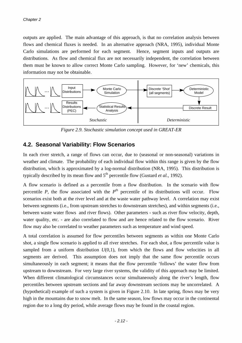
By means of Monte Carlo simulation, discrete ‘shots’ of the data and parameter set (e.g. flows,
process parameters, market data,...) are generated. With these discrete values, the entire geography
is simulated, using the deterministic model (Figure 2.9). In particular, discrete segment inputs and
Chapter 2
- 2.12 -
outputs are applied. The main advantage of this approach, is that no correlation analysis between
flows and chemical fluxes is needed. In an alternative approach (NRA, 1995), individual Monte
Carlo simulations are performed for each segment. Hence, segment inputs and outputs are
distributions. As flow and chemical flux are not necessarily independent, the correlation between
them must be known to allow correct Monte Carlo sampling. However, for ‘new’ chemicals, this
information may not be obtainable.
Monte CarloSimulation
DeterministicModel
Statistical ResultsAnalysis
Stochastic Deterministic
InputDistributions
ResultsDistributions
(PEC)
Discrete ‘Shot’(all segments)
Discrete Result
...
...
Figure 2.9. Stochastic simulation concept used in GREAT-ER
4.2. Seasonal Variability: Flow Scenarios
In each river stretch, a range of flows can occur, due to (seasonal or non-seasonal) variations in
weather and climate. The probability of each individual flow within this range is given by the flow
distribution, which is approximated by a log-normal distribution (NRA, 1995). This distribution is
typically described by its mean flow and 5th percentile flow (Gustard et al., 1992).
A flow scenario is defined as a percentile from a flow distribution. In the scenario with flow
percentile P, the flow associated with the Pth percentile of its distributions will occur. Flow
scenarios exist both at the river level and at the waste water pathway level. A correlation may exist
between segments (i.e., from upstream stretches to downstream stretches), and within segments (i.e.,
between waste water flows and river flows). Other parameters - such as river flow velocity, depth,
water quality, etc. - are also correlated to flow and are hence related to the flow scenario. River
flow may also be correlated to weather parameters such as temperature and wind speed.
A total correlation is assumed for flow percentiles between segments as within one Monte Carlo
shot, a single flow scenario is applied to all river stretches. For each shot, a flow percentile value is
sampled from a uniform distribution U(0,1), from which the flows and flow velocities in all
segments are derived. This assumption does not imply that the same flow percentile occurs
simultaneously in each segment; it means that the flow percentile ‘follows’ the water flow from
upstream to downstream. For very large river systems, the validity of this approach may be limited.
When different climatological circumstances occur simultaneously along the river’s length, flow
percentiles between upstream sections and far away downstream sections may be uncorrelated. A
(hypothetical) example of such a system is given in Figure 2.10. In late spring, flows may be very
high in the mountains due to snow melt. In the same season, low flows may occur in the continental
region due to a long dry period, while average flows may be found in the coastal region.

A Geo-referenced Aquatic Exposure Prediction Methodology for ‘Down-the-Drain’ Chemicals
- 2.13 -
alpine climate continental climate sea climate
Figure 2.10. Climatological differences in large river systems (example)
Within segments, the correlation between the waste water discharge flow and the ‘main river’ flow
is to be specified in the data set. For large rivers, it will generally be assumed that these flows are
uncorrelated. Dry weather waste water flow is obviously independent of the ‘main river’ flow. Wet
weather flow in combined sewers depends on short-term rain events, rather than longer-term
climatological conditions. One can expect the highest chemical fluxes to occur at high waste water
flows (e.g. due to treatment plant bypassing and combined sewer overflows). Hence, for chemical
risk assessment, the uncorrelated approach is probably the most appropriate, as it does not overlook
this worst-case scenario (high chemical loads combined with low river flows). For small rivers, on
the other hand, correlation of river flows with waste water discharge flows may become significant.
4.3. Uncertainty and Variability Analysis
4.3.1. Types of Uncertainty and Variability
The stochastic simulation in GREAT-ER deals with the major environmental variabilities
throughout the year(s) (especially focusing on river flows and climate) and the intrinsic variability
of parameters. Alternatively, it can also deal with parameter uncertainty within a fixed (i.e., non-
variable) scenario. Within the discussed simulation approach, four kinds of uncertainty and
variability can be discerned (Figure 2.11):
- Parameter Uncertainty and Variability. In reality, parameter values may vary considerably both
in time and in space, due to natural variability. Next to this, the actual parameter values and/or
distribution shapes are not known exactly. This uncertainty and/or variability may lead to
uncertainty and/or variability in the model results.
- Model Uncertainty. The applied model equations are not a full and completely correct
description of reality. Moreover, in the case of a geo-referenced model, the geographical
structure and segmentation of the simulated system may contain errors or strong simplifications.
- Simulation Uncertainty. In practice, the number of Monte Carlo shots is limited, due to the
required computation time. However, to obtain ‘perfect’ distributions, an infinite number of
shots would be needed. Even with more efficient sampling methods, the results distribution will
always be an approximation of the ‘true’ distribution. Next to this, specific mathematical /
numerical errors may occur during simulation.

Chapter 2
- 2.14 -
- Measurement Uncertainty (for model corroboration). The number of environmental samples,
which are used to develop temporal and spatial distributions of concentration, is necessarily
limited. Hence, the resulting measured distributions will only be an approximation of the true
distributions. Moreover, sampling and analytical variability will introduce further noise.
DATA
parameters,inputs
SIMULATION MODEL RESULTS
MEASUREMENTS
ParameterUncertainty
ModelUncertainty
SimulationUncertainty
MeasurementUncertainty
modelcorroboration
Figure 2.11. Types of uncertainty encountered in GREAT-ER (schematic)
In the example below (Figure 2.12), the shift and the difference in shape between the true
environmental concentration CENV and ‘ideal’ predicted concentration CPRED distributions can be
due to both parameter uncertainty and to model uncertainty. The fact that the real environmental
concentration CENV is a distribution rather than a single value, is due to natural variability. The
latter also determines (or at least influences) the shape of the measured $C ENV and computed $C PRED
distributions. Simulation uncertainty can be seen by comparing the ‘perfect’ CPRED with the Monte
Carlo simulation $C PRED. Measurement uncertainty is illustrated by the difference between the ‘real’
CENV and measured $C PRED.
In the stochastic simulation method described in this chapter, only parameter variability or
uncertainty are dealt with. Hence, neither model and simulation uncertainty, nor measurement
uncertainty are analyzed in the calculations.

A Geo-referenced Aquatic Exposure Prediction Methodology for ‘Down-the-Drain’ Chemicals
- 2.15 -
f
mg/L
CENV (real)
CENV (measured)
CPRED (perfect simulation)
CPRED (Monte Carlo)
REALITY MODEL
Figure 2.12. Measurement and predictive uncertainty (example frequency distributions)
4.3.2. Variability versus Uncertainty
Four classes of parameters can be defined, based on their degree of variability and/or uncertainty.
• Fixed Parameters. These parameters are constant in reality (i.e., they never change over time or
space). Moreover, their exact value is known. Hence, these parameters have no statistical
distribution. Typical examples are constants that are defined by laws of nature (e.g., the
universal gas constant R).
• Known Variability. These parameters have a natural variability in the environment. The exact
shape of their distributions is known, as well as the exact parameter values. Hence, the
uncertainty is negligible. Assuming that perfect measurements are available, a river flow
distribution built from a very long time-series of flow data could be an example of this class.
• Uncertainty. Some parameters are constant in reality (cf. the fixed parameters). However, their
exact value is not known. Their statistical distribution represents this uncertainty. An example
is the connection degree to waste water treatment in a specific area.
• Uncertainty and Variability. These parameters show a natural variability in the environment,
just like the ‘known’ variability parameters. But, neither the exact shape of their true
distribution nor the exact parameter values are accurately known. Hence, the parameters used to
describe the distributions of these parameters are distributions themselves. An example could
be river flow distributions predicted by a hydrological model.

Chapter 2
- 2.16 -
Variability analysis
One of GREAT-ER’s objectives is to provide high and low percentiles next to mean predicted
concentrations. The resulting frequency distribution at one point in a river represents the natural
variability of concentrations which is predicted to occur at that location. Such variability analysis
can be performed by means of a Monte Carlo simulation where all parameter variability is captured
in the parameters’ frequency distributions, and where the correlation between different parameters
has been accounted for. The resulting mean and percentile predicted concentrations are in
themselves point values, without any information about their confidence limits.
Uncertainty analysis
An uncertainty analysis can not be conducted simultaneously with a variability analysis using the
same Monte Carlo simulation (Ellis, 1998a). If the parameter frequency distributions include both
uncertainty and variability, this merely increases the spread of the distribution. It gives no extra
information about the confidence limits of the mean predicted concentration, and it gives an
under(over)estimation of low (high) percentiles. To conduct a combined uncertainty and variability
analysis, a two-stage approach is required (e.g. Cohen et al., 1996). In a first Monte Carlo
simulation, uncertainty is dealt with. For each uncertain parameter a point value is sampled from its
uncertainty frequency distribution. After this first Monte Carlo stage, a realization of the parameter
set has been created which is no longer influenced by uncertainty. This set is subsequently used in a
second variability Monte Carlo simulation. Finally, mean and confidence limits can be obtained for
mean predicted concentrations as well as for high and low percentiles. In a simplified way, this
method was implemented by Ellis (1998b) in the GUAVA approach.
A tentative theoretical uncertainty analysis for GREAT-ER simulations was worked out by Galoch
et al. (1998).
5. Simulation Software Design
The general software structure is shown in Figure 2.13. The simulator consists of the three sections:
Control Section, Data I/O Section and Model Section.
5.1. Control Section
The Control Section consists of two different hierarchical levels. In Level 1, the Monte Carlo
simulation is performed. First, the input parameters are obtained (by calling the Data I/O Section).
Second, a number of Monte Carlo simulation shots is generated. For each shot, a random ‘flow
percentile’ scenario is determined, discrete values are sampled from each parameter’s distribution,
and Level 2 of the simulation is called. After the Monte Carlo loop, the distribution parameters of
the results (e.g. mean and standard deviation) are calculated, from the ‘summary information’
provided by Level 2, and the simulation output is stored (by calling the Data I/O Section).

A Geo-referenced Aquatic Exposure Prediction Methodology for ‘Down-the-Drain’ Chemicals
- 2.17 -
Level 2, the Segments Loop level, applies to one discrete shot of the parameters set, which was
generated in Level 1. All segments are sequentially simulated, from the river network’s source to its
mouth. Influent data are prepared for each selected segment (from the interface variables), the input
parameters associated with the current segment are selected, and the current segment is simulated
(by calling the Model Section). After the segment’s simulation, its ‘summary variables’ are
calculated (WWTP influent and effluent concentration if applicable; river concentrations: start of
stretch, end of stretch, average value in stretch). Finally, the summary variables’ distribution
moments, which are needed to calculate the distribution parameters in Level 1, are updated.
CONTROL
sequential selectionof all
geographical segments
all segmentsinterface variables
Monte Carlo simulation(generation of parameter
& input data shots)
calculation ofselected segment
influent
all segmentssummary variables
parameters &input data shot for
all segments
selected segment’sinput data ¶meters
calculation ofresults distributions
input data & parameters distributions
resultsdistributions
MODEL
sequential selectionof all processes
ProcessSub-proc.
LEVEL
1
LEVEL
2
LOG device
DATA I/O
Figure 2.13. General software structure of the GREAT-ER chemical fate simulator

Chapter 2
- 2.18 -
5.2. Data I/O Section
The Data I/O Section is called from the Control Section. It is mainly used to read and interpret the
input provided by the geo-referenced and non-geo-referenced data banks, and to write the output
back to a geo-referenced results data bank. Also communication with the user (either through a log
file or via the user interface), and the processing of error messages are performed in this section.
5.3. Model Section
The Model Section is applied independently for each geographical segment. It is called from the
Control Section, from which it also receives all required input information and model parameters.
These represent a discrete case - no stochastics are incorporated here. The Model Section consists
of a Segment Control Section and one or more Processes. Each Process further consists of one or
more Sub-processes.
The Segment Control Section controls the simulation of an individual geographical segment. First,
it receives segment-specific input from the ‘main’ Control Section (see above). Then sequentially
all models applying to the different Processes and Sub-processes are called. Interface and summary
variables are calculated for the current segment, from the model state variables. Finally, the results
(i.e., the interface and summary variables) are sent back to the Control Section.
In Processes, which relate to individual processes occurring in a geographical segment, process-
specific input is received from the Segment Control Section, and sequentially all the required Sub-
Processes (one or several, depending on the process) are called. Model calculations are performed
(i.e., emission or removal are calculated), and the results (i.e. the model state variables) are sent
back to the Segment Control Section.
Sub-Processes relate to individual sub-processes within a specific Process. Here, sub-process-
specific input is received from the associated Process, process rate calculations are performed, and
the results (i.e., sub-process removal efficiencies) are sent back to the Process.
A Geo-referenced Aquatic Exposure Prediction Methodology for ‘Down-the-Drain’ Chemicals
- 2.19 -
6. Concluding Remarks
A geo-referenced simulation method for the prediction of aquatic exposure to individual ‘down-the-
drain’ chemicals was developed. The fate of these chemicals, taking into account emission, sewage
transport, treatment and river processes, is simulated by means of deterministic models. The natural
variability, and/or the uncertainty in the required information, is dealt with via a Monte Carlo
simulation. This finally results in statistical distributions of predicted concentrations, which can be
used for risk assessment.
A prototype of the presented simulation system was tested by means of a large sample data set,
containing 16,000 geographical segments. A 1,000 shot Monte Carlo simulation took less than 1.5
hours on a Windows NT workstation (Pentium, 150 MHz). Typical simulations for the GREAT-ER
pilot study catchments generally took less than 15-30 minutes. This indicates the feasibility of the
approach for detailed regional or large-scale pan-European simulations.

Chapter 3 -
Geo-referenced Prediction of EnvironmentalConcentrations of Chemicals in Rivers:
a Hypothetical Case Study
the contents of this chapter were published as:
Boeije, G. & Vanrolleghem, P. (1997). Geo-referenced prediction of environmental concentrationsof chemicals in rivers: a hypothetical case study. Forum for Applied Biotechnology. Mededelingen
Faculteit Landbouwwetenschappen, University Gent, 62(4b), 1599-1607.

- 3.1 -
Chapter 3
Geo-referenced Prediction of EnvironmentalConcentrations of Chemicals in Rivers:a Hypothetical Case Study
1. Introduction
For use within environmental risk assessment, a new tool for chemical fate prediction, GREAT-ER
(Geography-referenced Regional Exposure Assessment Tool for European Rivers), was developed.
In this chapter, the practical applicability of the GREAT-ER simulation methodology is illustrated
by means of a hypothetical but realistic case study. Temporal distributions of predicted
concentrations in the aquatic environment were calculated and analyzed. For the analysis of
seasonality (i.e., the variability of river flows through the year), the Monte Carlo simulation
technique was compared to a discrete ‘flow scenario’ approach. Finally, the scale-independent
character of the approach was investigated, by upscaling from a detailed to a larger geographical
scale.
The objectives of this hypothetical case study were: to demonstrate the practical applicability of the
GREAT-ER simulation approach, by modeling a virtual but realistic catchment; to analyze the
statistical distributions of predicted concentrations and to test the validity of the assumptions used in
the simulation approach; to compare the results of the Monte Carlo simulation approach with a
discrete flow scenario approach; and to investigate the options for upscaling the detail of a
catchment data set, from a small geographical scale to a large (aggregated) scale.
2. Model Implementation
A simple implementation of the simulation approach described in Boeije et al. (1997) was
developed to perform this hypothetical case study. A simplified waste water pathway structure and
low-complexity models were selected, as the objective was to demonstrate the feasibility of the
approach and its general behavior, rather than to analyze the potential accuracy of the predictions.
2.1. Waste Water Pathway Structure
The following processes were considered: domestic emission, combined sewers, waste water
treatment, and the river. Within one segment, these processes were interconnected as shown in
Figure 3.1.

Chapter 3
- 3.2 -
DomesticEmission
CombinedSewers
WWTP
River
untreated
upstream segments
downstream segments
treatment
Figure 3.1. Overview of processes within one segment
2.2. Models
2.2.1. Domestic Emission
Chemical mass fluxes were calculated from market data (product sold per person per year) and
population data. Domestic waste water flows (i.e. dry weather flows) were similarly derived from
daily water consumption and population.
Φoutdom M Pop= ⋅
⋅ ⋅
⋅1000
365 24 3600Q Q W Popout
domdwf= = ⋅
⋅ ⋅
⋅1
1000 24 3600[3.1]
2.2.2. Combined Sewer
No chemical elimination processes in the sewer system were considered. The combined sewer flow
was assumed to be related to the (calculated) dry weather flow. A correction factor α was used to
derive the sewer flow from this dry weather flow. If α < 1, leakages (out of the sewer) occur; if
α > 1, the waste water is diluted by rainfall or by infiltration of groundwater. It was further
assumed that α can be described by a log-normal distribution. For the given hypothetical case, the
mean was set to 1.5, while the 5th percentile was set to 1. This implies that the mean combined
sewer flow is 1.5 times its dry weather flow, while the 5th percentile low sewer flow is equal to the
dry weather flow.
Φ Φ Φinsewer
outsewer
outdom= = Q Q Qin
seweroutsewer
dwf= = ⋅α [3.2]
2.2.3. Waste water treatment
The treatment process consists of an untreated discharge model and a waste water treatment plant
(WWTP) model. The inflows are calculated as shown below:
Φ Φ
Φ Φinuntreat
outsewer
untreat
inwwtp
outsewer
wwtp
f
f
= ⋅
= ⋅
Q Q f
Q Q finuntreat
outsewer
untreat
inwwtp
outsewer
wwtp
= ⋅
= ⋅[3.3]
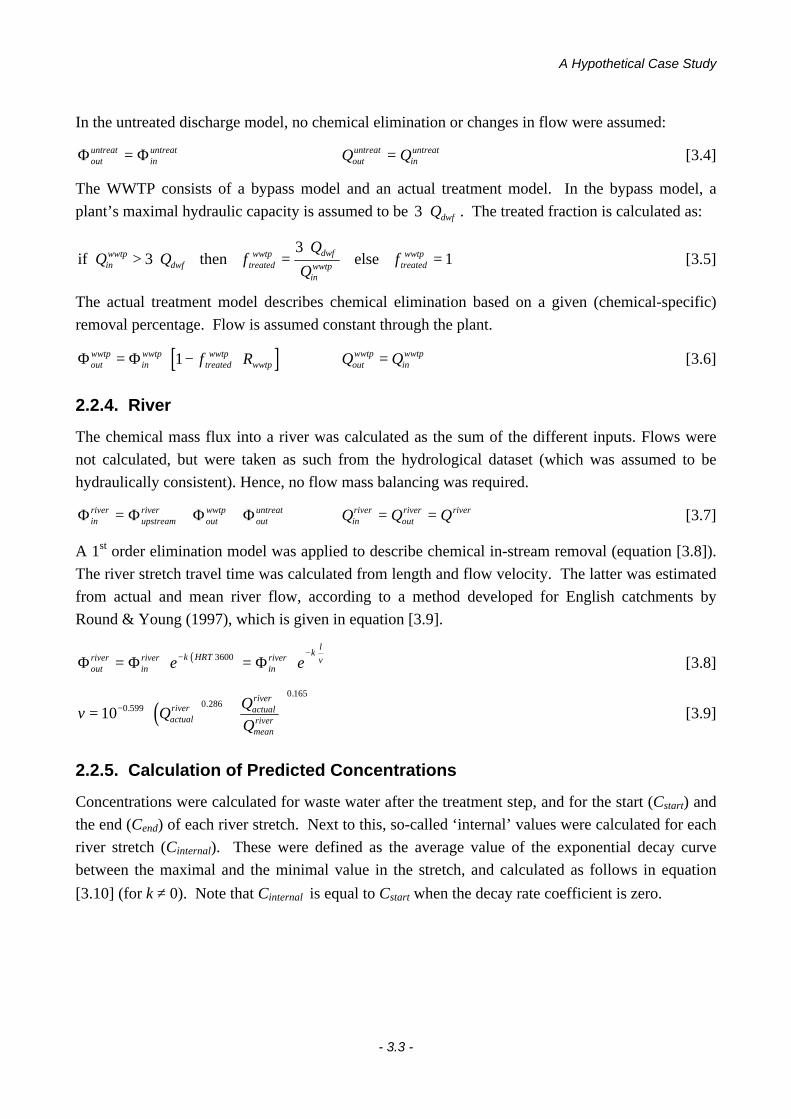
A Hypothetical Case Study
- 3.3 -
In the untreated discharge model, no chemical elimination or changes in flow were assumed:
Φ Φoutuntreat
inuntreat= Q Qout
untreatinuntreat= [3.4]
The WWTP consists of a bypass model and an actual treatment model. In the bypass model, a
plant’s maximal hydraulic capacity is assumed to be 3 ⋅ Qdwf . The treated fraction is calculated as:
if then else Q Q fQ
Qfin
wwtpdwf treated
wwtp dwf
inwwtp treated
wwtp> ⋅ =⋅
=33
1 [3.5]
The actual treatment model describes chemical elimination based on a given (chemical-specific)
removal percentage. Flow is assumed constant through the plant.
[ ]Φ Φoutwwtp
inwwtp
treatedwwtp
wwtpf R= ⋅ − ⋅1 Q Qoutwwtp
inwwtp= [3.6]
2.2.4. River
The chemical mass flux into a river was calculated as the sum of the different inputs. Flows were
not calculated, but were taken as such from the hydrological dataset (which was assumed to be
hydraulically consistent). Hence, no flow mass balancing was required.
Φ Φ Φ Φinriver
upstreamriver
outwwtp
outuntreat= + + Q Q Qin
riveroutriver river= = [3.7]
A 1st order elimination model was applied to describe chemical in-stream removal (equation [3.8]).
The river stretch travel time was calculated from length and flow velocity. The latter was estimated
from actual and mean river flow, according to a method developed for English catchments by
Round & Young (1997), which is given in equation [3.9].
( )Φ Φ Φoutriver
inriver k HRT
inriver k
l
ve e= ⋅ = ⋅− ⋅ ⋅ − ⋅3600 [3.8]
( )v QQQactual
river actualriver
meanriver= ⋅ ⋅
−10 0 599 0 286
0 165
. ..
[3.9]
2.2.5. Calculation of Predicted Concentrations
Concentrations were calculated for waste water after the treatment step, and for the start (Cstart) and
the end (Cend) of each river stretch. Next to this, so-called ‘internal’ values were calculated for each
river stretch (Cinternal). These were defined as the average value of the exponential decay curve
between the maximal and the minimal value in the stretch, and calculated as follows in equation
[3.10] (for k ≠ 0). Note that Cinternal is equal to Cstart when the decay rate coefficient is zero.

Chapter 3
- 3.4 -
( )
( )
( )
( )( )
( )( )
( )( )( )
C C e
CHRT
C e dt
CHRT k
e
CHRT k
ek
Ck HRT
e
end startk HRT
internal startk t
HRT
start k tHRT
start k HRT
start k HRT
= ⋅
⇒ =⋅
⋅ ⋅ ⋅
=⋅
⋅−
⋅
=⋅
⋅−
⋅ −−
⋅
=⋅ ⋅
⋅ −
− ⋅ ⋅
− ⋅
⋅
− ⋅⋅
− ⋅ ⋅
− ⋅ ⋅
∫
3600
0
3600
0
3600
3600
3600
1
3600
36001
36001 1
1
36001
[3.10]
2.3. Monte Carlo Simulation
By means of a 1,000 shot Monte Carlo simulation, the variability of the parameters mentioned in
Table 3.1 was incorporated into the simulation. The correlation between the river flow and the
combined sewer flow was assumed to be 0.6. This value was taken from the defaults used in the
SIMCAT model (NRA, 1995).
Table 3.1. Parameters used in Monte Carlo simulationParameter Description Distribution Correlation
to river flow
Qriver river flow lognormal 1
Rwwtp chemical elimination percentage in a WWTP normal 0
α combined sewer flow correction factor lognormal 0.6
3. Description of the Hypothetical Case Study
3.1. Hypothetical Catchment
A hypothetical but realistic catchment was constructed, which consists of a main river and one
tributary. Along the main river, there are two large cities (A and B), which discharge their waste
water into the river, after treatment or untreated. The tributary runs through a rural area with
disperse population, which discharge their untreated waste water directly into the tributary. A
representation of this catchment is given in the left half of Figure 3.2. The right half of the same
Figure shows the applied segmentation. A schematic representation, including segments
identification numbers (Segment ID), is given in Figure 3.3. Segments containing a waste water
input were labeled with ‘D’. The river stretches and waste water discharge properties are shown in
Table 3.2. For all discharges, the per capita water consumption was assumed to be 200 L/cap.day.
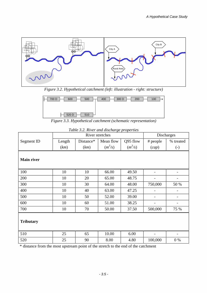
A Hypothetical Case Study
- 3.5 -
City A
City B
Rural Area
Figure 3.2. Hypothetical catchment (left: illustration - right: structure)
700 D 600 500 400 300 D 200 100
510520 D
Figure 3.3. Hypothetical catchment (schematic representation)
Table 3.2. River and discharge propertiesRiver stretches Discharges
Segment ID Length
(km)
Distance*
(km)
Mean flow
(m3/s)
Q95 flow
(m3/s)
# people
(cap)
% treated
(-)
Main river
100 10 10 66.00 49.50 - -
200 10 20 65.00 48.75 - -
300 10 30 64.00 48.00 750,000 50 %
400 10 40 63.00 47.25 - -
500 10 50 52.00 39.00 - -
600 10 60 51.00 38.25 - -
700 10 70 50.00 37.50 500,000 75 %
Tributary
510 25 65 10.00 6.00 - -
520 25 90 8.00 4.80 100,000 0 %
* distance from the most upstream point of the stretch to the end of the catchment

Chapter 3
- 3.6 -
3.2. Hypothetical Chemicals
Two hypothetical chemicals were defined: a conservative chemical A and a degradable chemical B.
The chemical properties and market information are given in Table 3.3.
Table 3.3. Chemical properties and market dataChemical A Chemical B
Product consumption 2 kg/cap.year 2 kg/cap.year
In-stream removal rate coefficient 0 h-1 0.069 h-1 ( t0.5 = 10 h )
WWTP elimination % 0 % ± 0 % 95 % ± 5 %
4. Results and Discussion
4.1. Predicted Concentrations
4.1.1. Main River Predicted Concentration Profiles
The main river predicted concentration profiles resulting from the hypothetical case simulation, are
shown in Figure 3.4.
The impact of the discharges of both cities is obvious. The tributary (at 40 km) results in a slight
decrease of the concentrations, which suggests that the tributary has a dilution effect on the main
river. The decrease after both cities is caused by increasing dilution and by in-stream-removal (for
Chemical B only).
4.1.2. Tributary
The mean and 95th percentile concentrations for the tributary mouth (and for the main river at the
same location) are given in Table 3.4 below.
Table 3.4. Tributary: predicted concentrations at the tributary mouth(and in main river at same location)
Chemical A Chemical B
Tributary Main River Tributary Main River
Cmean (mg/L) 0.699 0.627 0.082 0.085
C95%ile (mg/L) 1.082 0.816 0.086 0.109
The tributary’s dilution is sufficient to reduce its relative impact on the main river predicted
concentrations, as is shown for Chemical A. For Chemical B, concentrations are further reduced by
in-stream removal, and - even though the tributary receives the untreated waste water of 100,000
people - the tributary dilutes the main river.

A Hypothetical Case Study
- 3.7 -
Non Degradable Chemical
0
0.2
0.4
0.6
0.8
1
1.2
1.4
1.6
1.8
2
-80 -70 -60 -50 -40 -30 -20 -10 0
distance (km)
C (
mg
/L)
C mean
C 95%ile
Degradable Chemical
0
0.1
0.2
0.3
0.4
0.5
0.6
0.7
-80 -70 -60 -50 -40 -30 -20 -10 0
distance (km)
C (
mg
/L)
C mean
C 95%ile
Figure 3.4. Main river predicted concentration profiles
4.1.3. Discharges of Cities A and B
The mean and 95th percentile concentrations and chemical mass fluxes for both cities are given in
Table 3.5 below.
Table 3.5. Discharges of Cities A and B: concentrations and chemical mass fluxesChemical A Chemical B
City A City B City A City B
Predicted concentrations C
mean (mg/L) 27.4 27.4 7.69 13.9
95%ile (mg/L) 62.3 62.3 17.7 32.0
Predicted chemical mass fluxes Φmean (g/s) 31.7 47.6 9.43 25.3
95%ile (g/s) 31.7 47.6 12.0 27.9

Chapter 3
- 3.8 -
For the conservative Chemical A, the concentration distributions are identical for both cities, as
these values only depend on - assumed identical - market data and domestic water consumption.
For Chemical B, the uncertainty of the mass fluxes can be explained by the variability of WWTP
removal and plant bypassing.
Plant bypassing occurred in 82 of the 1000 Monte Carlo shots. As this is above the 5% threshold,
the 95th percentile concentrations of chemical B were influenced by these extreme flow events.
4.2. Analysis of Predicted Concentration Distributions (Chemical B)
For 3 locations in the study area, an analysis of the predicted concentration distributions of the
degradable Chemical B was made: the discharge (effluent) from City A, the mixing zone of this
discharge in the river, and the end of the catchment (segment 100) (see Figure 3.5).
Predicted concentration distributions are described by their mean and 95th percentile values. The
latter were obtained in 2 ways: (1) by assuming log-normality (using the method of moments), and
(2) by complete statistical analysis of the results dataset. Skewness of the distributions was also
determined. (Table 3.6). These distributions are illustrated by the histograms in Figure 3.5, together
with their geographical locations.
Table 3.6. Description of predicted concentration distributionsCity A
discharge
City A
mix. zone
End of
Catchment
Cmean (mg/L) 7.69 0.193 0.226
C95%ile assuming log-normality (mg/L) 17.75 0.269 0.271
C95%ile from statistical analysis (mg/L) 18.22 0.278 0.275
skewness - 2.37 0.76 0.39
The 95th percentile Cs calculated using the log-normality assumption corresponded well with the
true 95th percentiles. The skewness in the river was lower than in the discharge, due to leveling out
of high sewage concentrations by high river flows (the correlation between river and sewer flows
was 0.6). The lower skewness at the end of the catchment can be explained by leveling out due to
multiple discharges and the effect of in-stream removal.
A one-sample Kolmogorov-Smirnov test (SPSS Software version 7.5) for normality (on the
logarithms of the concentrations), using a significance threshold α = 0.05, showed that the log-
normality assumption for all three C distributions was valid.

A Hypothetical Case Study
- 3.9 -
City A - Discharge
0
50
100
150
200
250
2 4 6 8 10 12 14 16 18 20 22 24 26 28 30 32 34 36 38 40
Mor
e
C (mg/L)
Fre
qu
ency
0%
10%
20%
30%
40%
50%
60%
70%
80%
90%
100%
City A - Mixing Zone
0
20
40
60
80
100
120
140
160
0.09
0.10
5
0.12
0.13
5
0.15
0.16
5
0.18
0.19
5
0.21
0.22
5
0.24
0.25
5
0.27
0.28
5
0.3
0.31
5
0.33
0.34
5
0.36
0.37
5
0.39
0.40
5
Mor
e
C (mg/L)
Fre
qu
ency
0%
10%
20%
30%
40%
50%
60%
70%
80%
90%
100%
End of Catchment (after cities A and B)
0
50
100
150
200
250
0.09
0.10
5
0.12
0.13
5
0.15
0.16
5
0.18
0.19
5
0.21
0.22
5
0.24
0.25
5
0.27
0.28
5
0.3
0.31
5
0.33
0.34
5
0.36
0.37
5
0.39
0.40
5
Mor
e
C (mg/L)
Fre
qu
ency
0%
10%
20%
30%
40%
50%
60%
70%
80%
90%
100%
1 2
31
23
Figure 3.5. Predicted concentration distributions (histograms + geographical location)
4.3. Monte Carlo Simulation versus Flow Scenario Approach
An alternative to Monte Carlo simulation for dealing with flow seasonality, is the calculation of Cs
from discrete Flow Scenarios. In this case, one obtains a predicted concentration from a single
simulation at mean flow: C(Qm). From another simulation, at the 5th percentile flow, one obtains
C(Q95). Both calculation approaches were compared (using Cinternal values). The relative difference
of the discrete Cs at these two Flow Scenarios and the corresponding Monte Carlo simulation Cs is
shown in Figure 3.6.
Mean C and C at mean flow were very similar for all segments. In some cases, the predicted
concentrations at Q95 significantly under-estimated the 95th percentile C (10 - 15 % deviation).
From this, one can derive that the Flow Scenario approach can provide quick initial results
(especially for the means). For more detailed simulations, and especially for 95th percentiles, Monte
Carlo approach was better-performing. Note that for a complete uncertainty analysis, Monte Carlo
simulation is also required.
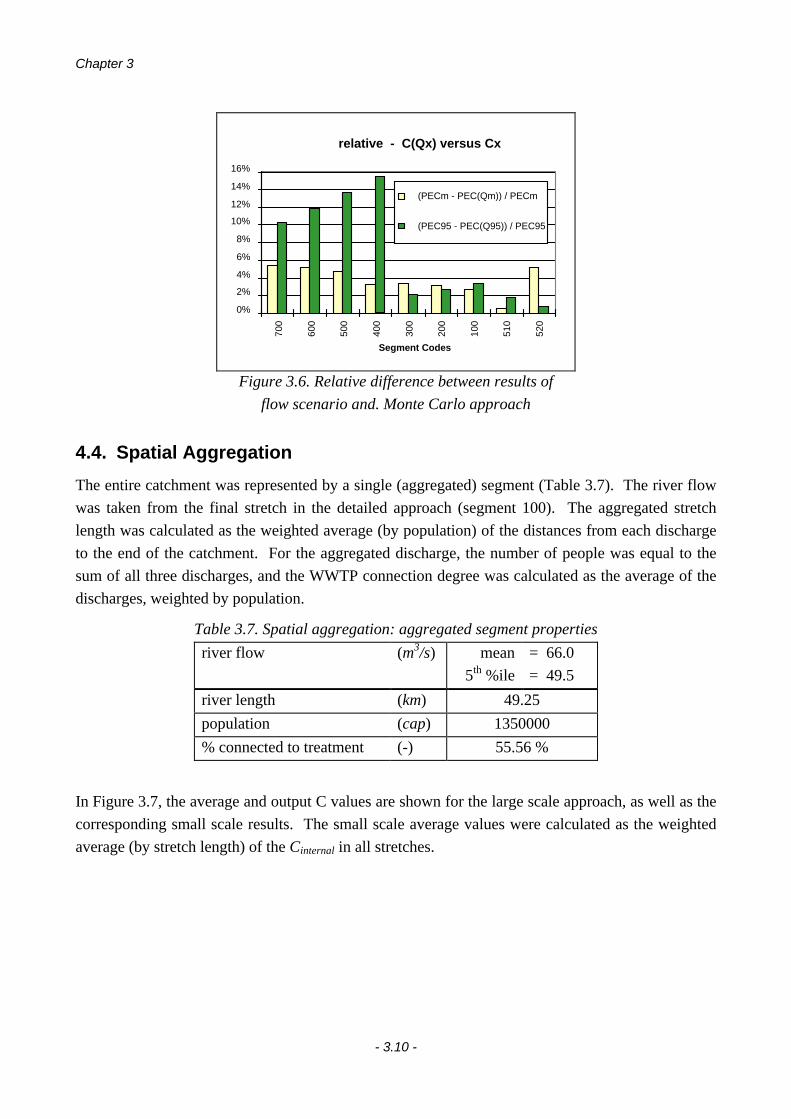
Chapter 3
- 3.10 -
relative - C(Qx) versus Cx
0%
2%
4%
6%
8%
10%
12%
14%
16%
700
600
500
400
300
200
100
510
520
Segment Codes
(PECm - PEC(Qm)) / PECm
(PEC95 - PEC(Q95)) / PEC95
Figure 3.6. Relative difference between results offlow scenario and. Monte Carlo approach
4.4. Spatial Aggregation
The entire catchment was represented by a single (aggregated) segment (Table 3.7). The river flow
was taken from the final stretch in the detailed approach (segment 100). The aggregated stretch
length was calculated as the weighted average (by population) of the distances from each discharge
to the end of the catchment. For the aggregated discharge, the number of people was equal to the
sum of all three discharges, and the WWTP connection degree was calculated as the average of the
discharges, weighted by population.
Table 3.7. Spatial aggregation: aggregated segment properties
river flow (m3/s) mean
5th %ile
= 66.0
= 49.5
river length (km) 49.25
population (cap) 1350000
% connected to treatment (-) 55.56 %
In Figure 3.7, the average and output C values are shown for the large scale approach, as well as the
corresponding small scale results. The small scale average values were calculated as the weighted
average (by stretch length) of the Cinternal in all stretches.

A Hypothetical Case Study
- 3.11 -
Large Scale versus Small Scale
0
0.1
0.2
0.3
0.4
0.5
average C(mean)
average C(95%ile)
output C(mean)
output C(95%ile)
C (
mg
/L)
Large Scale
Small Scale
Figure 3.7. Comparison of large scale versus small scale results
The large scale prediction for the catchment’s output C approximated the more detailed small scale
value within 12% (under-estimation). For the average predicted concentration of the entire
catchment, on the contrary, the large scale approach over-estimated the mean by 45% and the 95th
percentile by 36 %.
5. Conclusions
The GREAT-ER simulation approach allowed to analyze the impact of different discharges and
tributaries on the temporal and spatial distributions of predicted concentrations in a hypothetical
(but realistic) catchment. The resulting distributions were log-normal. For the prediction of 95th
percentile concentrations, Monte Carlo simulation was superior to the discrete Flow Scenario
approach. Also for a complete uncertainty or variability analysis, Monte Carlo simulation is needed.
However, to quickly obtain initial results, the Flow Scenario approach may be useful. Finally, it
was found that the GREAT-ER methodology allowed spatial aggregation of the simulated
hypothetical catchment, from a small detailed scale to a larger scale.

Chapter 4 -
Adaptation of the CAS Test System and SyntheticSewage for Biological Nutrient Removal
A significant part of this research was conducted at the Laboratory of Microbial Ecology
(Universiteit Gent), under the supervision of Prof. Dr. ir. W. Verstraete.
the contents of this chapter were published as:
Boeije, G., Corstanje, R., Rottiers, A. & Schowanek, D. (1998). Adaptation of the CAS test systemand synthetic sewage for biological nutrient removal. Part I: Development of a new syntheticsewage. Chemosphere, 38(4), 699-709.
Rottiers, A., Boeije, G., Corstanje, R., Decraene, K., Feijtel, T.C.J., Matthijs, E. & Schowanek, D.
(1998). Adaptation of the CAS test system and synthetic sewage for biological nutrient removal.Part II: Design and validation of test units. Chemosphere, 38(4), 711-727.
- 4.1 -
Chapter 4
Adaptation of the CAS Test System and SyntheticSewage for Biological Nutrient Removal
1. Introduction
Accurate exposure predictions are required for the environmental risk assessment of chemicals.
Determining the degree of elimination in waste water treatment plants is a crucial step in the
environmental exposure assessment of down-the-drain chemicals. To predict such removal
efficiencies, chemical fate models or laboratory simulation tests can be used. Even if mathematical
models are employed, laboratory tests are needed to provide the data necessary for model
calibration. In this chapter, an adaptation to the standard OECD CAS (Continuous Activated
Sludge) test (OECD, 1993; ISO, 1995) is presented, which incorporates biological nutrient removal.
In the scope of biodegradability testing of industrial chemicals, the EC directives 67/548/EEC
(CEC, 1967), 73/405/EEC (CEC, 1973) and their subsequent amendments specify the CAS test
system as one of the valid testing methodologies. The CAS system is probably the most widely
applied laboratory model for the simulation of activated sludge systems. Yet, many modern full-
scale wastewater treatment plants (WWTPs) can no longer be approached as a single aerated
reactor. The EU Urban Waste Water Treatment Directive 91/271/EEC (CEC, 1991) imposes
WWTP effluent criteria for nitrogen and phosphorus in nutrient sensitive areas. Full-scale
biological nutrient removal (BNR) designs such as the UCT, Biodenipho, Bardenpho, A/O, A2/O
process, etc., are being built with increasing fequency (Bowker & Stensel, 1990). Alternatively,
existing plants are retrofitted for BNR (e.g. Matsché, 1987; Randall et al., 1992; Kayser, 1994).
An improved laboratory-scale WWTP simulation system in which BNR is included would permit to
routinely study the degree of elimination of industrial chemicals, their biodegradation pathway(s) in
the different compartments, and potential effects on plant operation. Two aspects are of particular
interest:
1) the presence of alternative electron acceptors in addition to oxygen may lead to other
degradation pathways and/or kinetics under anoxic/anaerobic conditions.
2) two additional essential biological processes take place, i.e. excess phosphorus uptake, and
biological nitrogen removal via nitrification/denitrification. This may imply an increased
sensitivity of the plant to inhibitory substances (Kroiss et al., 1992, Strotmann & Eglsäer, 1995).
Chapter 4
- 4.2 -
In this chapter, two systems are evaluated and compared to the traditional CAS unit. In selecting
the test unit’s design, a number of factors were taken into account. The units were to be simple,
flexible, require little control, and be able to mimic most full scale plants built to meet the EU
Urban Waste Water Treatment Directive (CEC, 1991). To allow in-depth testing of the fate of
chemicals in activated sludge systems, they should also be fit for the use with radiolabeled test
compounds.
The OECD 303A protocol prescribes a synthetic sewage with a pre-established composition as
influent for the activated sludge units, whilst the latest ISO 11733 protocol permits the use of real
sewage. Although the results obtained from units run on synthetic sewage are intended to be highly
reproducible due to a minimized variability of the medium, the opposite is often seen in practice.
Despite close supervision of the units, the peptone and meat extract based OECD synthetic influent
often leads to a number of operational problems, such as frequent sludge bulking (AISE-CESIO
report, 1990, unpublished). The OECD feed has also been criticized that it is not an accurate
reflection of real domestic sewage due to its unbalanced composition, and therefore may result in a
decline in microbial diversity in the system (Kaiser et al., 1997). As such, not all catabolic enzyme
systems normally present in an activated sludge community would be expressed. With the use of
real domestic sewage the above problems can generally be overcome. However, domestic sewage is
prone to strong temporal variations in strength, and to occasional toxic pulses.
Recognizing the advantages a synthetic sewage can have in principle, this chapter introduces an
improved type of synthetic sewage. The starting point for its development was that it should be a
better simulation of real (pre-settled) sewage than the OECD medium, and that it should reduce the
latter’s inherent issues. A key success criterion for this new synthetic sewage was that it should
sustain the operation of a broad range of pilot scale wastewater treatment plants (WWTPs),
specifically those with biological nutrient removal (BNR), since these systems will increasingly
need to be simulated in the laboratory.
2. Adapted Test Units
2.1. Test Unit Selection
The ‘single sludge’ approach (i.e., the same activated sludge biomass circulating through all tanks
and redox zones) was selected, since this approach is by far the most popular for full-scale BNR
systems treating domestic sewage (Brett et al., 1997; Wentzel & Ekama, 1997).

Adaptation of the CAS Test System and Synthetic Sewage for Biological Nutrient Removal
- 4.3 -
The first unit, the commercially available Behrotest KLD4® (Behr unit) (Behr Labortechnik,
Düsseldorf-Reisholz, Germany), consists of an anoxic tank (4.2 L) in front of the aeration tank (4.5
L) (Figure 4.1). There is one sludge recycle, from the settler to the anoxic reactor. In this study the
sludge recycle rate was set at 2.5 times the influent flow. This system was initially designed for
biological nitrogen removal (Albertson & Stensel, 1994; Gronenberg & Schöberl, 1994), but luxury
P-uptake is not excluded (Kernn-Jespersen & Henze, 1993; Henze et al., 1995a; Barker & Dold,
1996). The Behr unit is not a sealed system, but it can be adapted for use with radiolabeled
chemicals.
The second unit was designed in-house, based on the University of Cape Town process (Ekama etal., 1984; Carucci et al., 1996; Barker & Dold, 1997; Brett et al., 1997). This unit was named
CAS-UCT. It consisted of three reactors in series: an anaerobic, an anoxic and an aerobic reactor
(Figure 4.1). The UCT process can be seen as a template for many single sludge BNR systems. Full
scale UCT plants have been built in several continents (Wentzel et al., 1988; Wentzel et al., 1992;
Randall et al., 1992; McClintock et al., 1993). The separation of the different redox zones in
distinct tanks makes this system attractive as a test unit.
Next to these BNR test units, the standard OECD CAS test unit was used as a reference.
2.2. Dimensioning of the CAS-UCT Test Unit
The CAS-UCT unit consists of an anaerobic, an anoxic and an aerobic tank, placed in series. There
are three recycle flows, which can be independently controlled. In designing the CAS-UCT unit, the
dimensions of the traditional CAS unit were taken as a starting point, i.e. the volume of the aerated
unit was set at 3.0 L. To determine the volumes of the other two tanks two scenarios were
compared, based on literature data (Ekama et al., 1984; Randall et al., 1992; Johanson, 1994): (1)
an anaerobic tank volume of 0.75 L and an anoxic tank of 1.5 L, and (2) both tanks with equal
volumes of 1.5 L.
Both scenarios, in combination with six different sludge recycling regimes, were evaluated
mathematically by means of the IAWQ Activated Sludge Model N° 2 (ASM2) (Henze et al.,1995b). As the ASM2 was primarily used as a design tool, the default parameter set (supplied by
Henze et al., 1995b) was used and no calibration of the model was performed. The model was
slightly modified: 50% of XS (the fraction of COD which biodegrades slowly) was assumed to be in
solution (i.e., not to be removed with settled sludge). For the settler, a simple mass-balance point
settler model was used. The fraction of solids washed out with the effluent was fixed at 0.5%. The
results of the ASM2 simulations (after having reached steady-state) are presented in Figure 4.2
below.

Chapter 4
- 4.4 -
Behr Unit
CAS-UCT Unit
CO2 traps
air
Figure 4.1. Schematic drawing of the CAS-UCT and Behr units

Adaptation of the CAS Test System and Synthetic Sewage for Biological Nutrient Removal
- 4.5 -
50%
55%
60%
65%
70%
75%
80%
85%
90%
95%
100%
2/2/
2
2/4/
2
2/1/
2
1/2/
2
4/2/
2
2/4/
1
2/2/
2
2/4/
2
2/1/
2
1/2/
2
4/2/
2
2/4/
1
Recycle Scenario (anox-anaer / aer-anox / settler-anox) (ratios relative to influent flow)
Rem
ova
l
N-removal
P-removal
Anaerobic V = 1.5 lAnaerobic V = 0.75 l
Figure 4.2. Influence of different design scenarios in the UCT unit on N and P removal
Based on the simulation results, the best performance was expected for scenario (2) with anaerobic
and anoxic volumes of each 1.5 L, together with a 2/2/2 recycle regime (i.e., the recycle flows from
the anoxic to the anaerobic tank, from the aerobic to the anoxic tank and from the settler to the
anoxic tank were all set to 2x the influent flow). The volume of the anaerobic tank was predicted to
have an important effect on P-removal, while the predicted impact on N-removal was very limited.
The recycle regime was expected to influence removal efficiency of both nutrients.
2.3. Test Unit Operation
2.3.1. Operating Conditions
The operating conditions for the BNR units are summarized in Table 4.1. The standard CAS unit
was operated in the uncoupled mode according to ISO (1995).
Influent flows were selected to have an HRT (Hydraulic Residence Time) in the aerobic tank of 6
hours (cf. the standard CAS test). The SRT (Sludge Residence Time) in the Behr and CAS-UCT
units was set at 15 or 20 days, to allow the development and maintenance of an adequate microbial
population (Focht & Verstraete, 1977; Henze et al., 1995a). At this SRT there still was sufficient
sludge wastage to ensure stable phosphorus (poly-P) removal with the sludge (CIWEM, 1994).
The sludge loading rate (BX) followed from the combination of reactor volumes, Mixed Liquor
Suspended Solids (MLSS) level, influent characteristics and flow rate, and was typically in the range
of 0.20-0.30 gCOD/gMLSS.day for the BNR systems.

Chapter 4
- 4.6 -
The sludge recycle ratio in the Behr unit (from the clarifier to the anoxic tank) was set to 2.5 times
the influent flow. For the CAS-UCT unit, the recycle regime presented in section 2.2 above was
used.
The dissolved oxygen (DO) concentration in the aeration tank of the Behr and CAS-UCT units was
aimed at 3.5 mg/L by tuning the aeration intensity. The safe working range was approximately 2.5
to 4.5 mg/L. A lower DO value would lead to anoxic conditions in the settler, resulting in sludge
rising due to denitrification, and P-release into the effluent. Higher DO levels were equally
undesirable, as the sludge was recycled to the anoxic and anaerobic tanks. DO levels above 0.2
mg/L in the latter would inhibit denitrification and P-release (Isaacs et al., 1994; Brett et al., 1997).
Under the operating conditions employed in this investigation, the DO concentration in the
anoxic/anaerobic tanks remained mostly below 0.1 mg/L.
All tests were performed at room temperature (18-23 °C). The influent pH was set at 7.25, and the
effluent pH was typically ranged between 7.5-7.9.
Table 4.1. Operating conditions for the BNR units
Volume(L)
HRT(h)
Run # MLSS(g/L)
SRT(d)
BX
(g/g.d)
Behr- Ax 4.2 5.6- A 4.5 6
#1 (a) 4.1 20 0.25#2 (a) 3.0 20 0.25#3 (b) 3.6 20 0.1-0.3#4 (a) 3.6 15 0.24
UCT- An 1.5 3- Ax 1.5 3 3.5 15 0.22- A 3 6
A = aerobic tank, Ax = anoxic tank, An = anaerobic tank, C = clarifier(a) synthetic medium, (b) real domestic sewage
2.3.2. Influent Characteristics
For most of the experiments with these units, synthetic sewage was used. As this was concurrently
under development during the experimental period, the units were operated using the precursor of
the Syntho medium (which is described later in this chapter). To compare the performance of a
Behr unit fed with synthetic sewage versus domestic waste water, the unit was also operated using
real domestic sewage as influent. The sewage used in this study was collected biweekly from the
Duffel domestic WWTP (Belgium) (passed through a sieve, mesh 0.5 mm). Average influent
characteristics for synthetic and domestic sewage are given in Table 4.2.

Adaptation of the CAS Test System and Synthetic Sewage for Biological Nutrient Removal
- 4.7 -
Table 4.2. Characterization of Syntho (precursor)and Duffel domestic sewage (values in mg/L)
Components Syntho (precursor) Domestic Sewage
Total COD 390 * 460 ± 200
Total Phosphorus 7.9 7 ± 3
Total Nitrogen 34.6 25 ± 7
pH 7.25 6.9 - 7.5
* calculated value
3. Development of a New Synthetic Sewage
3.1. Concept and Composition
Syntho was designed to mimic real pre-settled domestic wastewater. As it was intended to be used
as a standard influent to the Continuous Activated Sludge system (CAS), its components should be
commonly available and at a relatively low cost. In addition, the feed should be easy to prepare and
dose. The composition was chosen such that the use of Syntho would support excess N and P
removal, without aiming to maximize nutrient removal performance per se.
Syntho was conceived as a mixture of synthetic wastewater and a minor fraction (10% v/v) of pre-
settled real domestic wastewater. The selection of ingredients for the synthetic part was based on
the expected composition of domestic sewage. Syntho therefore differs considerably from classic
bacterial growth media. It was based on two fractions, a "sanitary" and a "household" wastewater
fraction. The sanitary fraction (black water) was based on the average composition and quantity of
sanitary wastewater, i.e. the combination of urine and feces (e.g. Hendericks, 1991; Yamada et al.,1991; Haubrich et al., 1994; Isselbacher et al., 1994). The household fraction (gray water) was
harder to define given its variability. A typical trait is that it contains biodegradable surface-active
agents.
The amount of biodegradable COD needed to transform 1 mg of NO3-N to N2 is 5.5-8.6 mg, and the
amount of biodegradable COD needed during biological P removal is 50-59 mg per mg of
phosphorus (Randall et al., 1992; US EPA, 1993; Henze et al., 1995a; Smolders et al., 1996).
Hence, to optimize the synthetic medium for biological nutrient removal, a COD:N:P ratio of
approximately 100:7:2 was chosen. A slight variability in this ratio occurs in practice due to the
mixing with real domestic sewage. Short chain volatile fatty acids such as acetate have a direct
impact on N and P removal (Isaacs & Henze, 1995; Zhao et al., 1995; Barker & Dold, 1996; Brett etal., 1997), and their level can be used to tune N and P removal to a desired level.

Chapter 4
- 4.8 -
The synthetic part also contains lyophilized sludge, mainly to act as a starter for floc formation.
Real sewage contains a particulate fraction which is inert or mineral. This fraction is simulated by
diatomaceous earth, which helps to increase sludge floc density. The type and concentration of
trace metals added to the medium is based on typical concentrations found in sewage (Kempton etal., 1987; Stephenson & Lester, 1987). An overview of the synthetic fraction (90%) of the Synthomedium is given in Table 4.3.
Table 4.3. Syntho medium composition (values in mg/L)
C-source N-source P-source Sewage simulation
Peptone 15 Urea 75 MgHPO4.3H2O 25 LAS * 10
Na-acetate** 120 NH4Cl 11 K3PO4.H2O 20 AE * 10
Dry meat extract 15 Uric acid 9 Lyophilised act.
sludge
50
Glycerol 40 Diatom. earth 10
Potato starch 50 Diet fibers 80
Milk powder 120
Minerals & Trace Metals ***
* C12-C14 Linear Alkylbenzene Sulphonate (LAS) and Alcohol Ethoxylate (e.g. C12-
C14AE5) or any other readily biodegradable surface active agents. For cost reasons the use
of a commercial rather than a pure grade is recommended (e.g. Fluka 48750 and 44200). ** Na-acetate can be varied to adjust the C/N/P ratio, to fine-tune N/P removal*** CaCl2, 5 mg/L; NaHCO3, 25 mg/L; FeSO4.7H2O, 10 mg/L; Trace metals: CuCl2.2H2O, 480
µg/L; CoCl2.6H2O, 50 µg/L; ZnCl2, 180 µg/L; MnSO4.H2O, 100 µg/L; K2MoO4, 20 µg/L;Cr(NO3)3.9H2O , 680 µg/L; NiSO4.6H2O, 300 µg/L; EDTA, 0.22 µg/L.
Domestic sewage provides a constant influx of bacteria and spores which act as an inoculum for the
activated sludge plant (Mara, 1974; Curds, 1975). The broad range of substrates in real sewage will
also ensure a diverse microbial population and enzymatic activity. To reduce the variability in
composition to a minimum, the amount of real sewage is limited to 10% v/v.
The total calculated and measured COD of the medium (without the 10% domestic sewage) are
approximately 470 and 508 mg/L., respectively. The alkalinity of the synthetic sewage was
determined by titration with 0.01 N HCl. At a set pH of 7.25, the alkalinity was 3.5 meq HCO3-/L.
In practice, a concentrated feed stock (e.g. 25 times) was prepared once, divided and frozen in small
portions, which were thawed and diluted with deionized water before use. All ingredients of the
feed stock were dissolved/mixed with deionized water. The lyophilized activated sludge and the diet
fibers were ground in a coffee mill prior to the mixing with water in order to avoid that particulate
materials would block the dosing pump. A stock solution of EDTA / trace metals in deionized
water (1000 times more concentrated) was prepared separately, stored in a refrigerator, and mixed
with the synthetic sewage to the required concentration on the day of use.

Adaptation of the CAS Test System and Synthetic Sewage for Biological Nutrient Removal
- 4.9 -
The cost of Syntho in terms of chemical ingredients is low, ca. 0.03 Euro per liter, or 3.5 - 4.5 Euro
per week of testing for a CAS test.
The concentrated feed and the dilution water / real sewage were dosed separately. Although
separate dosing of a concentrated stock solution is technically more complicated, this procedure was
preferred because it enabled to keep the synthetic feed stock stable for several days on the laboratory
bench, resulting in a constant and well defined organic load to the test units. Compared to the
traditional OECD feed, the absence of bad odors produced by degrading constituents was an
additional advantage.
The experiments with the test units were conducted using the precursor of Syntho as influent. This
medium contained (in mg/L): urea 75; ammonium chloride 11; uric acid 9; dried yeast 45; lauric
acid 25; Na-acetate 68; diet fiber 35; LAS 10; AE 10; meat extract 15; peptone 15; starch 70; low
fat milk powder 80; mineral salts and trace elements as in Syntho.
3.2. Simulation Experiments
3.2.1. ASM2 Parameterization
The ASM2 (Henze et al., 1995b) was used to predict the operation of the test units fed with the
proposed medium composition. The same modifications as described in section 2.2 were applied.
The ASM2 model components are divided into solubles (S) and particulates (X), which are further
subdivided into easily biodegradable, fermentable and other components. The different constituents
of Syntho were assigned to an ASM2 component based on the degradation steps they are assumed to
undergo in the units (Table 4.4). These were derived from literature data (Mandelstam &
Halvorson, 1960; Eastman & Fergusson, 1981; Henze & Mladenovsi, 1991; Eliosov & Argaman,
1995; Mino et al., 1995).
To further characterize the Syntho-related input parameters for ASM2, a respiration test was carried
out with the synthetic sewage according to the methodology described by Spanjers (1993), Spanjers
et al. (1994) and Henze et al.(1995a). Endogenously-respiring sludge was fed with a pulse dose of
Syntho. The calculations were made according to the methodology described by Spanjers &
Vanrolleghem (1995) and Henze et al. (1995a). The readily and slowly biodegradable fractions
could be derived from the respiration curve. The inert fraction was obtained from the difference
between the calculated COD and the actual oxygen demand. It is then further subdivided into a
soluble inert fraction (Si), which was obtained from the effluent COD values of a test unit operating
on Syntho and an inert particulate fraction (Xi).

Chapter 4
- 4.10 -
The respiration curve obtained for the synthetic medium Syntho is shown in Figure 4.3. this
compares well with the respirograms obtained by Spanjers & Vanrolleghem (1995) for real
domestic sewage. Based on the respirogram, a characterisation of the synthetic medium was carried
out, as presented in Table 4.4 (column ‘Syntho - measured’). The main differences between Synthoand real sewage are that the fraction of ‘heterotrophic bacteria’ is larger in real sewage, while
Syntho contains somewhat more ‘soluble fermentation substrate’ (e.g. glycerol, surfactants, uric
acid, and possibly part of the peptone and meat extract) as well as ‘soluble fermentation products’
(i.e. acetate). The amount of ‘heterotrophic bacteria’ in Syntho might be underestimated, since the
medium was freshly prepared and the lyophilized biomass was probably not fully active when added
to the respirometer. The OECD medium has a predominant (estimated) component of Xs, which is
not truly particulate, but refers to the easily accessible colloidal peptone and meat extract fraction.
0
10
20
30
40
50
60
70
80
90
100
0 20 40 60 80 100 120 140 160 180 200
Time (min)
Oxygen Uptake Rate (mg/L.h)
Figure 4.3. Respiration curve obtained with the Syntho medium

Adaptation of the CAS Test System and Synthetic Sewage for Biological Nutrient Removal
- 4.11 -
Table 4.4. Estimated and measured ASM2 parameters for the Syntho medium
Description Syntho(measured)
Syntho(estimated)
OECD
(estimated)
Real
sewage**
Si Inert soluble matter 0.00 0.04 0.00 0.06
Sa Soluble fermentation products 0.14 0.18 0.00 0.08
Sf Soluble fermentation substrate 0.21 0.25 0.19 0.16
Xs Slow biodegradable partic. matter 0.52 0.43 0.81 0.50
Xaut Autotrophic bacteria * 0 0 0
Xpha Cell internal storage * 0 0 0
Xpao P-accumulating organisms * 0 0 0
Xh Heterotrophic bacteria 0.04 0.03 0.00 0.10
Xi Inert particulate matter 0.09 0.07 0.00 0.10* not measured; ** from range given in Henze et al. (1995b)
3.2.2. ASM2 Simulation
A simulation with the ASM2 was carried out to illustrate the expected differences in unit
performance when a laboratory UCT system is fed with the OECD medium versus Syntho. The
composition of the sewage, and in particular the COD:N:P ratio as well as the quantity of readily
biodegradable matter, is the main factor in determining whether a UCT unit will perform well
(Ekama et al., 1984; Tam et al., 1992; Fass et al., 1994; Henze et al., 1995a; Qasim et al., 1996;
Randall et al., 1992).
To evaluate the performance of the new medium, ASM2 simulations were carried out for the UCT
test unit described higher in this chapter. For this simulation, a sludge loading rate of 0.25
kgCOD/kgMLSS.day was used. The sludge residence time was set to 15 days, and all three sludge
recycles were fixed at 2.5 times the influent flow. The experimentally determined model
components were used for Syntho. The simulation results are presented in Figure 4.4.
Treating domestic sewage a full-scale UCT will typically give an efficiency in the range of 87-90%
P-removal, and up to 75-80% N-removal (Randall et al., 1992). The ASM2 predicts that a UCT test
unit operated on Syntho could achieve a similar performance. When comparing Syntho with the
OECD medium, it appeared that the OECD medium supports a predicted N removal in the order of
65-70%. This is slightly lower than the 70-75% predicted with Syntho. The OECD medium would
support only 55-60% biological P removal, while with Syntho this was predicted to reach 85-90%.
These differences can be ascribed to the improved COD:N:P ratio of Syntho, and the presence of
acetate to stimulate BNR processes.

Chapter 4
- 4.12 -
0%
20%
40%
60%
80%
100%
0 5 10 15
Removal
Time (days)
OECD medium
Syntho medium
N removal
P removal
Figure 4.4. ASM2 simulation: predicted N and P removal in a UCT unit during startup
4. Analytical Methods
The parameters outlined below were monitored on a daily basis during working days. Samples were
taken from the influent and the effluent of the units. The effluent was collected over a period of at
least one hour.
For COD, nitrogen (total, ammonia, nitrate and nitrite) and phosphorus (total phosphate)
measurements the Dr. Lange spectrophotometric analytical test system LASA 20 (Dr. Bruno Lange
GmbH) was employed.
Mixed liquor suspended solids (MLSS) were measured according to the Dutch NEN-norm 6445;
both the aeration tank and the anoxic/anaerobic tanks were sampled. The Sludge Volume Index
(SVI) was measured in a 1-litre Imhoff cone over a period of 30 minutes with sludge from the
aeration tank. Dissolved Oxygen (DO) was measured on a daily basis in the aeration tank, in the
anoxic tank and in the sludge layer of the settler. pH was monitored in all reactors as well as in the
influent tank to ensure that the acidification of the sewage did not result in an excessively low pH of
the influent. The temperature in the aeration tank was measured each working day. Influent flow
rates and the sludge recycling flow rates were verified at least once a week.
LAS was measured by a specific HPLC method according to Matthijs & De Henau (1987).

Adaptation of the CAS Test System and Synthetic Sewage for Biological Nutrient Removal
- 4.13 -
5. Results and Discussion
5.1. Reactor Performance
In a first series of tests the Behr-, CAS-UCT and standard CAS units were compared in terms of
COD, N and P removal, as a validation procedure for the BNR systems. No test chemicals were
dosed in this round of testing. ASM2 predictions were used to cross-check the observed test units’
performance.
5.1.1. Reactor Performance with Synthetic Medium
Figure 4.5 compares the average COD, N and P removal performance for the three units fed with
Syntho (precursor) synthetic medium. The test conditions are given in Table 4.1 (Run #1 for the
Behr unit). Results relate to a measurement period of minimum three weeks of steady-state
operation after initial start-up and equilibration. After inoculation of the units with nitrifying
activated sludge it typically took 2-4 weeks to obtain stable reactor performance in terms of nutrient
removal.
As the graphs indicate, both the Behr and the CAS-UCT unit are capable of excess nitrogen and
phosphorus removal, while the standard CAS unit does not achieve more than ca. 30% N and P
elimination. The measured removal in the BNR units is in line with the expectations of what can be
achieved with laboratory-scale units (Carucci et al., 1996) and what is seen in full-scale plants
(Bowker & Stensel 1990; Randall et al., 1992; Kuba et al., 1993).
The ASM2 predictions (Figure 4.5) concur with the experimentally obtained values. ASM2 was
very accurate at predicting the level of N and C removal in all systems. The P removal rate was
slightly underestimated for the Behr and CAS-unit, and slightly overestimated for the UCT. In
terms of residual COD levels in the effluent, the CAS, Behr and CAS-UCT performed similarly,
with average concentrations of 15.8, 16.2 and 13.0 mg/L respectively.
The observation of a high degree of P-removal in the Behr-unit, which was considered in first
instance a nitrogen removal system, is noteworthy. It should be seen in the light of the recent
literature (e.g. Barker & Dold, 1996), which indicates that a significant fraction of the poly-P
bacteria can use nitrate as electron acceptor and develop into an active population in the anoxic
reactor.

Chapter 4
- 4.14 -
ASM2 predictions
Experimental results
0%
20%
40%
60%
80%
100%
CAS Behr CAS-UCT
Phosphorus removal
0%
20%
40%
60%
80%
100%
CAS Behr CAS-UCT
Nitrogen removal
100%
0%
20%
40%
60%
80%
CAS Behr CAS-UCT
COD removal
Figure 4.5. Test unit performance using the Syntho (precursor) medium
5.1.2. Behr Unit Performance: Domestic versus Synthetic Sewage
For the Behr unit, a comparison in terms of BNR and reactor stability was made between real
domestic sewage and the precursor of the Syntho medium. The operating conditions are given in
Table 4.1 (Behr: Run #2 and #3).
Reactor performance
The COD, N and P removal data are shown in Figure 4.6, for the period after day 30 of each
experiment. Average removal values are given in Table 4.5. For COD and N-removal, the Behr-
unit performed on average quite similarly on synthetic and real sewage. However, the synthetic feed
showed a lower P-removal. The COD:N:P ratio for the Duffel raw sewage was in the range of
100:6:1.5 while that for Syntho’s precursor was ~100:9:2. Hence, for the unit operating on domestic
sewage more volatile fatty acids were available for phosphate removal, which would otherwise be
used during denitrification (Fass et al., 1994).
Table 4.5. Performance of the Behr unit: % COD, N and P removal
Syntho (precursor) Duffel sewage
COD 95.0 ± 3.0 92.5 ± 5.0
N 76.0 ± 8.0 73.0 ± 6.0
P 70.0 ± 9.0 91.0 ± 8.0

Adaptation of the CAS Test System and Synthetic Sewage for Biological Nutrient Removal
- 4.15 -
Days
0 5 10 15 20 25 30 35
0
20
40
60
80
100COD % removal
Days0 5 10 15 20 25 30 35 40
0
20
40
60
80
100COD % removal
Days0 5 10 15 20 25 30 35
0
20
40
60
80
100Nitrogen % removal
Days
0 5 10 15 20 25 30 35
0
20
40
60
80
100Nitrogen % removal
Days0 5 10 15 20 25 30 35
-100-80-60-40-20020406080
100120
Measured ASM2 prediction
0 5 10 15 20 25 30 35 400
20
40
60
80
100
Days
Phosphorus % removalPhosphorus % removal
Duffel Domestic Sewage Syntho (precursor) Synthetic Medium
Figure 4.6. Performance of the Behr unit: synthetic medium vs. Duffel sewage

Chapter 4
- 4.16 -
The drop in performance of the unit fed with Duffel sewage (after ten days) was probably caused by
a toxic pulse, in combination with a rainy period (causing a low-strength influent). A similar
performance upset was also recorded in the Duffel treatment plant itself. The temporary high
dilution caused a low level of easily biodegradable carbon and resulted in a net phosphate release, as
predicted by the ASM2. However, the drop in nitrogen and COD removal cannot be ascribed to
dilution, and was hence not predicted by the ASM2. This event illustrates the vulnerability of the
N-removal sub-process (i.e. nitrification/denitrification) to occasional presence of toxic substances,
and the relative time frame needed for the BNR processes to recover. It also illustrates an inherent
disadvantage of using real sewage.
While the N- and P-removal were relatively well predicted by the ASM2, COD removal seemed to
be underestimated systematically. Although the Duffel wastewater is mainly domestic, it also
contains the effluent of an ice cream factory. Because of this, there may have been a larger than
typical fraction of readily biodegradable organic matter, leading to a somewhat higher COD
removal. Note that this may also explain the excellent P-removal.
Sludge settling
Bulking sludge is a major concern in waste water treatment, and can also disturb laboratory tests. It
may lead to a severe reduction in unit performance as sludge is lost in the effluent and the system
becomes operationally unstable. The sludge settling properties were compared between the
synthetic medium and real sewage (Figure 4.7).
A different SVI trend was observed for the two feeds. The SVI of sludge fed with real sewage only
rose slightly during the test (from ca. 140 to 180 mL/g). The SVI of the sludge fed with synthetic
medium remained stable within a similar range for ca. 1 month, but afterwards it deteriorated to ca.
270 mL/g. This caused no operating problems, but it suggested that the medium could still be
improved to prevent sludge bulking. It should be mentioned here that full scale BNR plants have
been reported to suffer frequently from bulking and/or foaming sludge (Casey et al., 1992; Urbain etal., 1993). Randall et al. (1992) quoted an SVI of 120 mL/g as typical for a well functioning full-
scale system with N and P removal.

Adaptation of the CAS Test System and Synthetic Sewage for Biological Nutrient Removal
- 4.17 -
Time (days)0 10 20 30 40 50
SVI (ml/g MLSS)
120
140
160
180
200
220
240
260
280
300
Duffel sewage
Syntho medium(precursor)
Figure 4.7. SVI - Behr unit Run #2 (Syntho precursor medium and Duffel sewage)
Reformulated Syntho Medium
The above considerations led to the reformulation of the Syntho medium to its final composition,
described in section 3. The COD:N:P ratio was changed to 100:7:2 (instead of 100:9:2). The
acetate level was increased, to drive the BNR processes. Furthermore, to stimulate floc formation
and increase floc density, dried yeast was replaced by lyophilized activated sludge, and
diatomaceaous earth was added.
Later experiments using the Syntho medium (which are not described in this thesis) indicated an
improvement of P-elimination (79.6% ± 17.5% in a Behr unit, 77.1% ± 8.8% in a UCT unit) and
sludge settling (SVI in a UCT unit of 173 mL/g on average, over a 40 day test period).
5.2. LAS Removal in the Test Units
Primary removal of LAS was measured in the three units. Experimental conditions are given in
Table 4.1 (Run #4 for the Behr unit, using the Syntho medium).
A parent LAS removal efficiency of 99.4% ± 0.1% was found for the Behr-unit. For the CAS-UCT
unit, the primary LAS removal was also found to be 99.4% (single measurement). The OECD
303A CAS unit was observed to have 98.6% ± 0.8% parent LAS removal.
The units with BNR performed better than the standard CAS test in terms of LAS removal. This is
thought to be caused in first instance by the longer HRT and SRT. It needs to be assessed further
whether the presence of different redox environments, and the possibility of additional biochemical
pathways, may have contributed in any way to the higher chemical removal efficiencies.

Chapter 4
- 4.18 -
6. Conclusions
Both the CAS-UCT and the Behr-unit are easy to handle laboratory scale BNR simulation systems,
which could be included in standard testing, complementary to the CAS system. They can be
operated on Syntho or on real domestic wastewater (tested for the Behr-unit) in a stable way with
minimal extra costs or effort compared to the standard CAS system.
Under the investigated test conditions, a similar degree of COD, N and P removal was achieved
with both BNR units. The Behr-unit was observed to be a simple and reliable system, providing all
basic BNR functionality; the CAS-UCT unit is in principle a more versatile tool, but it is also more
complex. The experimental nutrient removal results corresponded well with ASM2 predictions for
both units.
A dissatisfaction with the OECD synthetic sewage and the need for a synthetic medium which
supports BNR in lab-scale units resulted in the development of a more realistic synthetic feed for
use in standard WWTP simulation tests. Based on a literature review, a new medium (Syntho) was
developed, consisting of a blackwater (sanitary) and a greywater (household) fraction next to 1/10
real sewage. A respiration test indicated that the new medium is a reasonable approximation of real
domestic sewage. Although sludge settling was superior when real sewage was used, the SVI with
the synthetic sewage remained sufficiently low to permit a stable test duration of 1 to 3 months.
The longer HRT and SRT applied in the BNR systems led to a reduction in effluent levels of
biodegradable chemicals like the surfactant Linear Alkylbenzene Sulphonate (LAS) compared to the
CAS test. The role of the system’s different redox zones in the overall removal requires further
investigation for various types of chemicals.

Chapter 5-
Adaptation of the SimpleTreat Chemical FateModel to Single-Sludge Biological Nutrient
Removal Waste Water Treatment Plants
a condensed version of this chapter was published as:
Boeije, G., Schowanek, D. & Vanrolleghem, P. (1998). Adaptation of the SimpleTreat chemical fatemodel to single-sludge biological nutrient removal waste water treatment plants. Water Science
and Technology 38(1), 211-218.
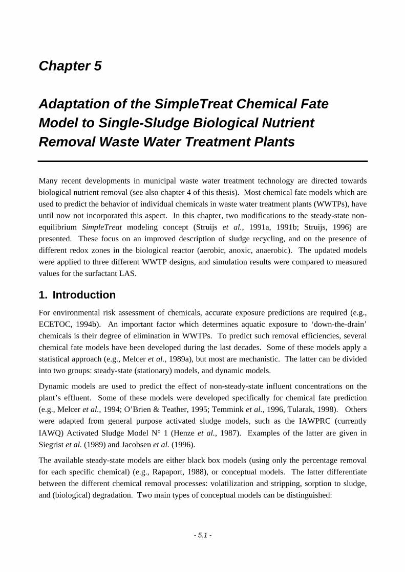
- 5.1 -
Chapter 5
Adaptation of the SimpleTreat Chemical FateModel to Single-Sludge Biological NutrientRemoval Waste Water Treatment Plants
Many recent developments in municipal waste water treatment technology are directed towards
biological nutrient removal (see also chapter 4 of this thesis). Most chemical fate models which are
used to predict the behavior of individual chemicals in waste water treatment plants (WWTPs), have
until now not incorporated this aspect. In this chapter, two modifications to the steady-state non-
equilibrium SimpleTreat modeling concept (Struijs et al., 1991a, 1991b; Struijs, 1996) are
presented. These focus on an improved description of sludge recycling, and on the presence of
different redox zones in the biological reactor (aerobic, anoxic, anaerobic). The updated models
were applied to three different WWTP designs, and simulation results were compared to measured
values for the surfactant LAS.
1. Introduction
For environmental risk assessment of chemicals, accurate exposure predictions are required (e.g.,
ECETOC, 1994b). An important factor which determines aquatic exposure to ‘down-the-drain’
chemicals is their degree of elimination in WWTPs. To predict such removal efficiencies, several
chemical fate models have been developed during the last decades. Some of these models apply a
statistical approach (e.g., Melcer et al., 1989a), but most are mechanistic. The latter can be divided
into two groups: steady-state (stationary) models, and dynamic models.
Dynamic models are used to predict the effect of non-steady-state influent concentrations on the
plant’s effluent. Some of these models were developed specifically for chemical fate prediction
(e.g., Melcer et al., 1994; O’Brien & Teather, 1995; Temmink et al., 1996, Tularak, 1998). Others
were adapted from general purpose activated sludge models, such as the IAWPRC (currently
IAWQ) Activated Sludge Model N° 1 (Henze et al., 1987). Examples of the latter are given in
Siegrist et al. (1989) and Jacobsen et al. (1996).
The available steady-state models are either black box models (using only the percentage removal
for each specific chemical) (e.g., Rapaport, 1988), or conceptual models. The latter differentiate
between the different chemical removal processes: volatilization and stripping, sorption to sludge,
and (biological) degradation. Two main types of conceptual models can be distinguished:

Chapter 5
- 5.2 -
• One type focuses on the mass-balancing of individual waste water treatment sub-processes. This
was applied by e.g. Blackburn & Troxler (1984), Namkung & Rittmann (1987), Melcer et al.(1989b), Govind et al. (1991), Cowan et al., (1993b), Monteith et al. (1993), ECETOC (1994c),
Melcer et al. (1994), van Wijk et al. (1996), McAvoy et al., (1997), Lee et al. (1998). In a
simplified way, this approach was also used by Birch (1991), only considering chemical removal
via biodegradation.
• In a second type, “diffusive” chemical transport is driven by the non-equilibrium between
chemical fractions in different phases. Fugacity calculations (after Mackay & Paterson, 1981 and
1982) are used for this purpose. This approach was applied by e.g. Struijs et al. (1991a, 1991b),
Clark et al. (1995), and Struijs (1996).
The existing steady-state WWTP fate models are typically based on ‘standard’ plant configurations,
designed in first instance for carbon removal. However, nowadays biological nutrient removal has
become an important aspect in municipal waste water treatment and water quality management
(e.g., CEC, 1991). Many WWTPs in Europe are upgraded to include nitrogen and phosphorus
removal, or will be in the near future. Hence, it is warranted to include the effect of nutrient
removal processes on chemical fate.
In this chapter, a modification of the SimpleTreat model is presented, which describes chemical fate
(as parent removal) in typical single-sludge biological nutrient removal WWTPs. In the modified
model, an improved description of sludge recycling is used, and the presence of different redox
zones is taken into account. Additionally, the calculation of several plant design and operation
parameters was revised.
2. Process Description
2.1. Activated Sludge Plant Configuration
2.1.1. General
In most of the above mentioned steady-state activated sludge models, the modeled plant consists of
a primary settler, a completely mixed aeration tank, and a secondary settler. Some models allow to
disregard the primary settler (e.g., Struijs, 1996). Others allow to consider several aeration basins in
series (e.g., Melcer et al., 1994). In the model presented here, the primary settler is considered a
separate module, and was not included as a part of the activated sludge model itself. A scheme of
this configuration is given in Figure 5.1.
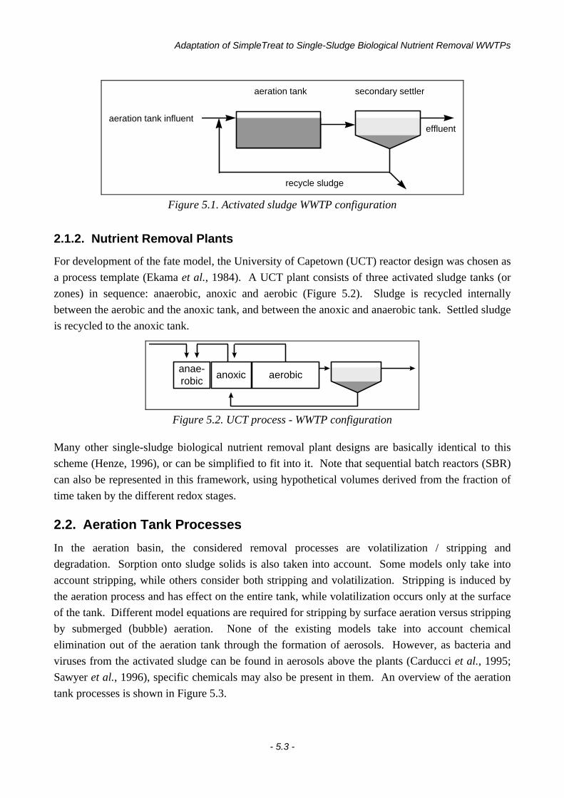
Adaptation of SimpleTreat to Single-Sludge Biological Nutrient Removal WWTPs
- 5.3 -
secondary settleraeration tank
recycle sludge
aeration tank influenteffluent
Figure 5.1. Activated sludge WWTP configuration
2.1.2. Nutrient Removal Plants
For development of the fate model, the University of Capetown (UCT) reactor design was chosen as
a process template (Ekama et al., 1984). A UCT plant consists of three activated sludge tanks (or
zones) in sequence: anaerobic, anoxic and aerobic (Figure 5.2). Sludge is recycled internally
between the aerobic and the anoxic tank, and between the anoxic and anaerobic tank. Settled sludge
is recycled to the anoxic tank.
anae-robic
anoxic aerobic
Figure 5.2. UCT process - WWTP configuration
Many other single-sludge biological nutrient removal plant designs are basically identical to this
scheme (Henze, 1996), or can be simplified to fit into it. Note that sequential batch reactors (SBR)
can also be represented in this framework, using hypothetical volumes derived from the fraction of
time taken by the different redox stages.
2.2. Aeration Tank Processes
In the aeration basin, the considered removal processes are volatilization / stripping and
degradation. Sorption onto sludge solids is also taken into account. Some models only take into
account stripping, while others consider both stripping and volatilization. Stripping is induced by
the aeration process and has effect on the entire tank, while volatilization occurs only at the surface
of the tank. Different model equations are required for stripping by surface aeration versus stripping
by submerged (bubble) aeration. None of the existing models take into account chemical
elimination out of the aeration tank through the formation of aerosols. However, as bacteria and
viruses from the activated sludge can be found in aerosols above the plants (Carducci et al., 1995;
Sawyer et al., 1996), specific chemicals may also be present in them. An overview of the aeration
tank processes is shown in Figure 5.3.
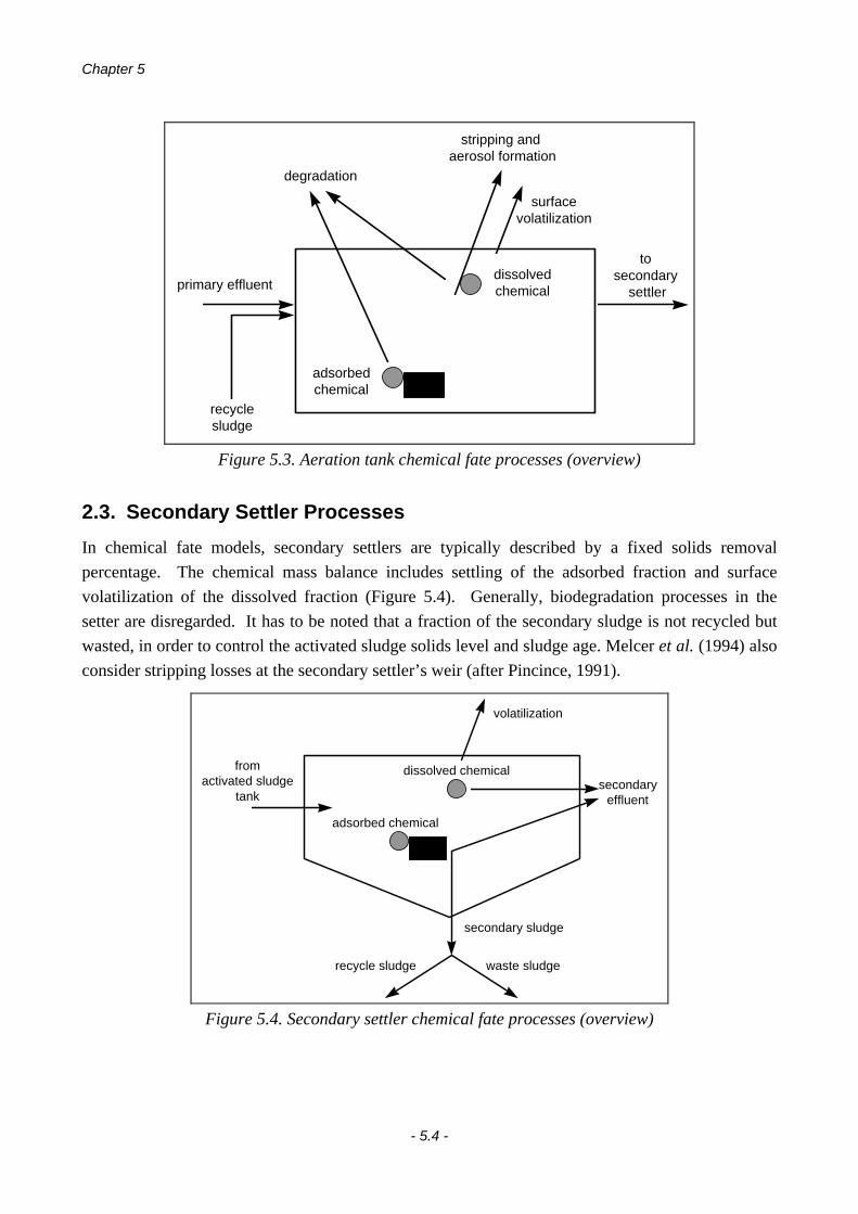
Chapter 5
- 5.4 -
dissolvedchemical
adsorbedchemical
surfacevolatilization
stripping and aerosol formation
degradation
primary effluent
recyclesludge
to secondary
settler
Figure 5.3. Aeration tank chemical fate processes (overview)
2.3. Secondary Settler Processes
In chemical fate models, secondary settlers are typically described by a fixed solids removal
percentage. The chemical mass balance includes settling of the adsorbed fraction and surface
volatilization of the dissolved fraction (Figure 5.4). Generally, biodegradation processes in the
setter are disregarded. It has to be noted that a fraction of the secondary sludge is not recycled but
wasted, in order to control the activated sludge solids level and sludge age. Melcer et al. (1994) also
consider stripping losses at the secondary settler’s weir (after Pincince, 1991).
dissolved chemical
adsorbed chemical
fromactivated sludge
tanksecondary
effluent
secondary sludge
volatilization
recycle sludge waste sludge
Figure 5.4. Secondary settler chemical fate processes (overview)

Adaptation of SimpleTreat to Single-Sludge Biological Nutrient Removal WWTPs
- 5.5 -
3. Modeling Approach
3.1. Model Selection
The current state of the art in steady-state WWTP fate models is mainly represented by TOXCHEM(Melcer et al., 1994), AS-TREAT (McAvoy et al., 1997) and the model by Lee et al. (1998), and
SimpleTreat (Struijs et al., 1991a, 1991b; Struijs, 1996). The latter was chosen as a starting point
for the development of a nutrient removal plant model, because of the inherent flexibility of its
fugacity approach, and because of its regulatory acceptance within European Union risk assessment
(e.g., Vermeire et al., 1997).
3.2. The SimpleTreat Concept
The SimpleTreat model was developed by Struijs et al. in 1991, mainly for regulatory purposes.
Several modifications and improvements to the model and its assumptions were suggested, e.g. by
Cowan et al. (1993), Mikkelsen et al. (1996), Jacobsen et al., (1996). Based on these comments, a
revised version was designed by Struijs (1996).
In the SimpleTreat approach, a WWTP is represented by a number of compartments (boxes). Each
chemical phase (dissolved, sorbed) in each reactor is assigned one box. A standard carbon removal
plant (without considering primary settling) consists of 6 boxes: air above the WWTP, dissolved
and sorbed chemical in the activated sludge tank, dissolved and sorbed chemical in the settler, and
sorbed chemical in the settled sludge. Mass balancing for all boxes is performed using the
SIMPLEBOX method (van de Meent, 1993). The mass balance for each box i is:
mass change = - elimination - outflux to other boxes - outflux out of the system
+ influx from other boxes + influx into the system
or:
( ) ( )VdCdt
k C V ADV XCH C ADV XCH Cii
i i i i j i j ij
outi
j i j i jj
ini⋅ = − ⋅ ⋅ − + ⋅ − + + ⋅ +
= =∑ ∑, , , ,
1
6
1
6
Φ Φ [5.1]
At steady state, continuous and constant influxes into and outfluxes out of the system are assumed.
The change in concentration dCi/dt is zero. Hence, the mass balance equation for box i can be
written as:
( ) ( )k C V ADV XCH C ADV XCH Ci i i i j i j ij
outi
j i j i jj
ini⋅ ⋅ + + ⋅ + − + ⋅ =
= =∑ ∑, , , ,
1
6
1
6
Φ Φ [5.2]
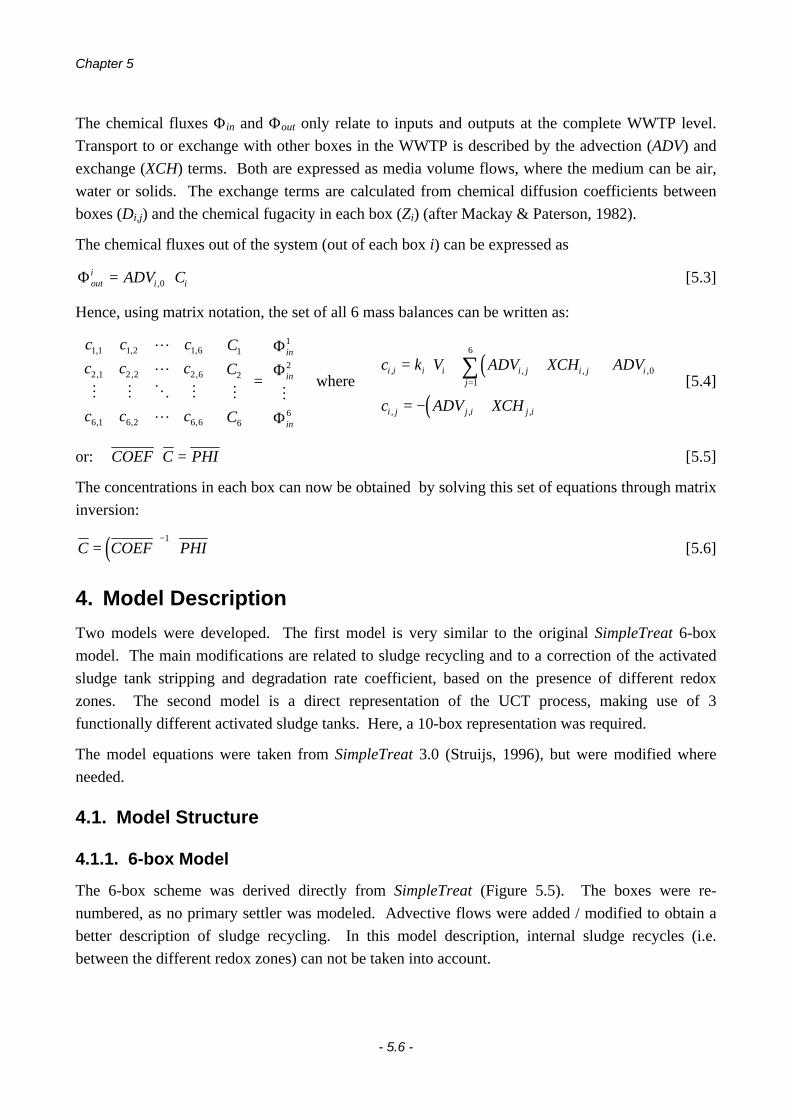
Chapter 5
- 5.6 -
The chemical fluxes Φin and Φout only relate to inputs and outputs at the complete WWTP level.
Transport to or exchange with other boxes in the WWTP is described by the advection (ADV) and
exchange (XCH) terms. Both are expressed as media volume flows, where the medium can be air,
water or solids. The exchange terms are calculated from chemical diffusion coefficients between
boxes (Di,j) and the chemical fugacity in each box (Zi) (after Mackay & Paterson, 1982).
The chemical fluxes out of the system (out of each box i) can be expressed as
Φouti
i iADV C= ⋅,0 [5.3]
Hence, using matrix notation, the set of all 6 mass balances can be written as:
c c c
c c c
c c c
C
C
C
in
in
in
1 1 1 2 1 6
2 1 2 2 2 6
6 1 6 2 6 6
1
2
6
1
2
6
, , ,
, , ,
, , ,
L
L
M M O M
L
M M
⋅
=
ΦΦ
Φ
where ( )
( )
c k V ADV XCH ADV
c ADV XCH
i i i i i j i jj
i
i j j i j i
, , , ,
, , ,
= ⋅ + + +
= − +
=∑
1
6
0[5.4]
or: COEF C PHI⋅ = [5.5]
The concentrations in each box can now be obtained by solving this set of equations through matrix
inversion:
( )C COEF PHI= ⋅−1
[5.6]
4. Model Description
Two models were developed. The first model is very similar to the original SimpleTreat 6-box
model. The main modifications are related to sludge recycling and to a correction of the activated
sludge tank stripping and degradation rate coefficient, based on the presence of different redox
zones. The second model is a direct representation of the UCT process, making use of 3
functionally different activated sludge tanks. Here, a 10-box representation was required.
The model equations were taken from SimpleTreat 3.0 (Struijs, 1996), but were modified where
needed.
4.1. Model Structure
4.1.1. 6-box Model
The 6-box scheme was derived directly from SimpleTreat (Figure 5.5). The boxes were re-
numbered, as no primary settler was modeled. Advective flows were added / modified to obtain a
better description of sludge recycling. In this model description, internal sludge recycles (i.e.
between the different redox zones) can not be taken into account.

Adaptation of SimpleTreat to Single-Sludge Biological Nutrient Removal WWTPs
- 5.7 -
air
aeration tankdissolved
aeration tankadsorbed to SS
secondary settlerdissolved
secondary settleradsorbed to SS
secondary settlersettled
activ
ated
slu
dge
influ
ent
efflu
ent
secondary waste sludge
1
diffusive exchangeelimination
2
3
4
5
6
0
Figure 5.5. Nutrient removal WWTP fate model - 6-box
4.1.2. 10-box Model
The 10-box model scheme is shown in Figure 5.6. Each of the three activated tanks was represented
by 2 boxes (dissolved and sorbed phase). All possible sludge recycles (from the settler as well as
internal recycles) were implemented. Note that in practice only a limited number of all possible
sludge recycles are to be used (as shown in Figure 5.6 for the standard UCT design).
efflu
ent
air
anaerobic tankdissolved
adsorbed to SS
sec. settlerdissolved
sec. settleradsorbed to SS
sec. settlersettled
activ
ated
slu
dge
influ
ent
secondary waste sludge
1
2
3
8
9
10
0
anoxic tankdissolved
anoxic tankadsorbed to SS
4
5
aerobic tankdissolved
aerobic tankadsorbed to SS
6
7
advective transportdiffusive exchangeeliminationnot used in UCT
Figure 5.6. Nutrient removal WWTP fate model - 10-box

Chapter 5
- 5.8 -
4.2. Influent Calculation
The influent consist of a dissolved and an adsorbed chemical fraction. The influent enters the
treatment system simultaneously into box 2 and box 3 (for both the 6-box and the 10-box model).
Other boxes receive no influent flux. If no primary settler is present, the dissolved and sorbed
fraction of the influent are assumed to be in complete equilibrium (cf. Struijs, 1996). If a primary
settler model is connected in front of the activated sludge model, the dissolved/sorbed fractionation
of the settler model is used to calculate the secondary influent partitioning.
4.3. Advective Transport
4.3.1. 6-box Model
In SimpleTreat, only the solids phase of the recycled sludge is considered. Moreover, different
sludge recycle flows and recycling ratios cannot be taken into account. As in nutrient removal
processes sludge recycling is crucial, a more realistic description of these recycles was included into
the model. It was assumed that the interstitial water phase of the settled sludge is identical to the
main water phase in the settler (box 4). Hence, the water phase of the sludge recycle could be
represented by an advective transport of settler water to the activated sludge tank (ADV4,2). The
activated sludge tank’s flow balance was corrected for this additional inflow, by modifying the term
ADV2,4. To take into account the actual recycle flow of the solids phase, the ADV3,5 term was also
updated.
Air advection
- into / out of area above WWTP: ADV ADV h v A Aair wind act sludge sec0 1 1 0, , .= = ⋅ ⋅ + [5.7]
Water volume flow rate
- WWTP in/outflow: ADV ADV Q0 2 4 0, ,= = [5.8]
- sludge propagation: ( )ADV Q R2 4 1, = ⋅ + [5.9]
- settled sludge recycle: ADV Q R4 2, = ⋅ [5.10]
An additional advective flow term (ADV2,1) may be added to describe the transport of water droplets
out of the activated sludge tank through aerosol formation.

Adaptation of SimpleTreat to Single-Sludge Biological Nutrient Removal WWTPs
- 5.9 -
Solids volume flow rate
- WWTP in/outflow: ADV QSSsewage
solidssewage0 3 610, = ⋅
⋅ ρ[5.11]
ADV QSSeffluent
solidsML5 0 610, = ⋅
⋅ ρ[5.12]
- settled sludge recycle: ADV ADV ADV6 3 5 6 6 0, , ,= − [5.13]
- sludge propagation: ( )ADV Q RSSML
solidsML3 5 6
110, = ⋅ + ⋅
⋅ ρ[5.14]
- sludge settling: ADV ADV ADV5 6 3 5 5 0, , ,= − [5.15]
- sludge waste: ADV surplusSS
solidsML6 0 610, =
⋅Φ
ρ[5.16]
4.3.2. 10-box Model
Air advection
- into / out of area above WWTP: ADV ADV h v A Aair wind act sludge sec0 1 1 0, , .= = ⋅ ⋅ + [5.17]
Water volume flow rate
- WWTP in/outflow: ADV ADV Q0 2 8 0, ,= = [5.18]
- internal sludge recycles: ADV Q Ranox anaer4 2, ,= ⋅ [5.19]
ADV Q Raer anaer6 2, ,= ⋅ [5.20]
ADV Q Raer anox6 4, ,= ⋅ [5.21]
- settled sludge recycles: ADV Q RS anaer8 2, ,= ⋅ [5.22]
ADV Q RS anox8 4, ,= ⋅ [5.23]
ADV Q RS aer8 6, ,= ⋅ [5.24]
- sludge propagation: ( )ADV Q R R RS anaer aer anaer anox anaer2 4 1, , , ,= ⋅ + + + [5.25]
( )( )
ADV Q R R R
Q R R Q R
S anaer aer anaer anox anaer
S anox aer anox anox anaer
4 6 1, , , ,
, , ,
= ⋅ + + +
+ ⋅ + − ⋅ 5. ]
( )= ⋅ + + + +Q R R R RS anaer S anox aer anaer aer anox1 , , , ,

Chapter 5
- 5.10 -
( )( )
Q R R R
R Q R
anaer S aer anaer anox
S aer anaer anox
8, , , , ,
, , ,
= ⋅ + + + +
+ ⋅ − ⋅ + 5. ]
( )= ⋅ + + +Q R R RS anaer S anox S aer1 , , ,
Solids volume flow rate
- WWTP in/outflow: QSS
3 6= ⋅
⋅ ρ[5.28]
ADVSSeffluent
solidsML9 610, [ .29
- internal sludge recycles: ADV ADV anoxic
solidsML5 3 2 6,= ⋅
⋅ ρ[5.30]
ADV ADVSSaerobic
solidsML7 3 6 2 610, ,= ⋅
⋅ ρ[5.31]
ADV ADVSSaerobic
solidsML7 5 6 4 610, ,= ⋅
⋅ ρ[5.32]
- settled sludge recycles: ADV RS anaer10 3, ,= ⋅ζ [5.33]
ADV RS anox10 5, ,= ⋅ζ [5.34]
ADV RS aer10 7, ,= ⋅ζ [5.35]
with ζ =−
+ +ADV ADV
R R RS anaerobic S anoxic S aerobic
9 10 10 0, ,
, , ,
- sludge propagation: ADV ADVSSanaerobic
solidsML3 5 2 4 610, ,= ⋅
⋅ ρ[5.36]
ADV ADVSSanoxic
solidsML5 7 4 6 610, ,= ⋅
⋅ ρ[5.37]
ADV ADVSSaerobic
solidsML7 9 6 8 610, ,= ⋅
⋅ ρ[5.38]
- sludge settling: ADV ADV ADV9 10 7 9 9 0, , ,= − [5.39]
- sludge waste: ADV surplusSS
solidsML10 0 610, =
⋅
Φ
ρ[5.40]

Adaptation of SimpleTreat to Single-Sludge Biological Nutrient Removal WWTPs
- 5.11 -
4.4. Diffusive Exchange
4.4.1. Calculation of Fugacities and Box Volumes
For the calculation of the diffusive exchanges, the fugacity approach is applied. The fugacities of
the different media have to be known, as well as the volumes of the different compartments.
Fugacities
Struijs et al. (1991a, 1991b) derived expressions for fugacity calculations from Mackay and
Paterson (1982):
- air: ( )Zt
airair
=⋅ +
1
273R[5.41]
- water: ZHwater =1
[5.42]
- mixed liquor (act. sludge): ZK
HMLdML
solidsML
=⋅ ρ
[5.43]
Box volumes (6-box model)
- air above the WWTP: ( )V A A hact sludge sec air1 = + ⋅. [5.44]
- activated sludge tank (water phase): V Vact sludge2 = . [5.45]
- activated sludge tank (solids phase): V VSS
act sludgeML
solidsML3 610
= ⋅⋅. ρ
[5.46]
- secondary settler (water phase): V Vsec4 = [5.47]
- secondary settler (solids phase):( )
V VR SS
sec
secSS
ML
solidsML5 6
1
10= ⋅
− ⋅
⋅ ρ[5.48]
The volume of compartment 6 (secondary sludge thickening layer) need not be known by the model.
Box volumes (10-box model)
Similar calculations as in the 6-box model are used for the 10-box model volumes. Obviously the
box numbering is different.
- air above the WWTP: ( )V A A hact sludge sec air1 = + ⋅. [5.49]

Chapter 5
- 5.12 -
- activated sludge tank (water phase): V V fact sludge anaerobic2 = ⋅. [5.50]
V V fact sludge anoxic4 = ⋅. [5.51]
V V fact sludge aerobic6 = ⋅. [5.52]
- activated sludge tank (solids phase): V V fSS
act sludge anaerobicanaerobic
solidsML3 610
= ⋅ ⋅⋅. ρ
[5.53]
V V fSS
act sludge anoxicanoxic
solidsML5 610
= ⋅ ⋅⋅. ρ
[5.54]
V V fSS
act sludge aerobicaerobic
solidsML7 610
= ⋅ ⋅⋅. ρ
[5.55]
- secondary settler (water phase): V Vsec8 = [5.56]
- secondary settler (solids phase):( )
V VR SS
sec
secSS
aerobic
solidsML9 6
1
10= ⋅
− ⋅
⋅ ρ[5.57]
As in the 6-box model, the volume of the secondary sludge thickening layer (compartment 10) is not
required.
4.4.2. Diffusive Chemical Exchange
The diffusion coefficient for chemical exchange between two boxes i and j is expressed in terms of
first order kinetics, after Mackay and Paterson (1982):
D Dk
V Z V Z
i j j idiff
i i j j
, ,= =
⋅+
⋅1 1
[5.58]
Then, the exchange from box i to j, expressed as medium volume flow rate, is calculated as:
XCHD
Zi ji j
i,
,= [5.59]
Sludge / water exchange
Between the dissolved and the adsorbed phases in the activated sludge tank and in the secondary
settler, non-equilibrium partitioning is described, in terms of first order (de-)sorption kinetics (cf.
[5.58]):

Adaptation of SimpleTreat to Single-Sludge Biological Nutrient Removal WWTPs
- 5.13 -
- activated sludge tank (mixed liquor): [5.60]
(additional terms for 10-box model between square brackets)
[ ] [ ][ ] [ ]
D D D D D Dk
V V V Z V V V Z
act sludgesorb
water ML
2 3 4 5 6 7 3 2 5 4 7 6
2 4 6 3 5 7
1 1, , , , , ,., , , ,
, , , ,
= =
⋅+
⋅
and [ ] [ ]XCH XCH XCH
D D D
Zwater2 3 4 5 6 7
2 3 4 5 6 7, , ,
, , ,, ,, ,
=
[ ] [ ]XCH XCH XCH
D D D
ZML3 2 5 4 7 6
3 2 5 4 7 6, , ,
, , ,, ,, ,
=
- secondary settler: [5.61]
(alternative terms for 10-box model between brackets)
( ) ( )( ) ( )
D D D Dk
V V Z V V Z
secsorb
water ML
4 5 8 9 5 4 9 8
4 8 5 9
1 1, , , ,= =
⋅+
⋅
and ( ) ( )XCH XCH
D D
Zwater4 5 8 9
4 5 8 9, ,
, ,=
( ) ( )XCH XCH
D D
ZML5 4 9 8
5 4 9 8, ,
, ,=
The applied kinetic rate coefficients for sorption / desorption are given in Table 5.1 (taken from
Struijs, 1996).
Table 5.1. Sorption/desorption kinetic rate coefficients
Half-life (s) 1st order rate coefficient (s-1)
Activated sludge tank kact sludgesorb
.360 1.925 10-3
Secondary settler ksecsorb 3600 192.5 10-6
Air / water exchange
Activated sludge tank
For the activated sludge tank(s), two types of air-water exchange are considered: surface
volatilization (without the impact of aeration) and stripping (due to aeration). Stripping can be due
to either surface aeration (surface impellers) or (submerged) bubble aeration. The modeling
approach is based on the two-layer model (Liss and Slater, 1974; Mackay and Leinonen, 1975).

Chapter 5
- 5.14 -
6-box model
Only the aerobic (fraction of the) activated sludge tank is aerated. Hence a correction factor for the
tank volume which undergoes stripping is taken into account. The diffusion coefficients and
exchange terms for air / water exchange in the activated sludge tank are calculated as shown below
in [5.62]. The surface volatilization term (right) was not changed compared to SimpleTreat. In the
stripping term (left), both the tank volume and the tank surface area were corrected for the aerobic
fraction, finally leading to the aerobic fraction term in the numerator.
( ) ( )D D
k
Vf A
AZ
f V Z
k
VA
AZ
V Z
f k k
VA
AZ
V Z
str
aerobic act sludge
totalair
aerobic water
v
act sludge
totalair
water
aerobic str v
act sludge
totalair
water
1 2 2 1
1
21
2
12
1 1 1 1
1 1
, ,
. .
.
= =
⋅⋅
⋅
+⋅ ⋅
+
⋅ ⋅+
⋅
=⋅ +
⋅ ⋅+
⋅
[5.62]
and XCHD
Zair1 2
1 2,
,=
XCHD
Zwater2 1
2 1,
,=
Like in Struijs (1996), the surface volatilization rate coefficient kv is estimated as:
kh
Kh
KK
K
vair
H
act sludge
air
H
water
=+
+
1
1. [5.63]
Compared to Struijs (1996), two modifications were made to the calculation of the stripping rate
coefficient kstr. First, the total activated sludge tank volume was replaced by the aerobic volume.
Second, the calculation of oxygen requirement was adjusted (see below, section 4.6).
The calculation of the stripping rate coefficient depends on the type of aeration: surface aeration
versus bubble aeration:

Adaptation of SimpleTreat to Single-Sludge Biological Nutrient Removal WWTPs
- 5.15 -
- surface aeration (after Roberts et al., 1984; Munz & Roberts, 1989):
( ) ( )k GPC
OxReq
f HRT DO DO
HPa
m molGPC
HPa
m molGPC
k ak a
K
k ak a
K
KK
strsurface
aerobic act sludge sat
G
LH
G
LH
H
H
= ⋅ ⋅⋅ ⋅ ⋅ −
≥ ⇒ =
< ⇒ =⋅
⋅ +≅
⋅⋅ +
Ψ3600
250 1
2501
4040 1
3
3
.
[5.64]
- bubble aeration (after Hsieh et al., 1993):
kOxReq
f VHstr
bubble
aerobic act sludge
= ⋅ ⋅⋅
⋅−0 89 10 3 1 04..
. [5.65]
It has to be noted that the Oxygen Requirement (OxReq) concept (as for surface aeration) is used in
the bubble aeration stripping model, rather than the per capita bubble aeration rate (Gcap) which is
used in SimpleTreat.
10-box model
The calculation of the diffusion coefficients and exchange terms for air / water exchange in the
different activated sludge tanks are given below. Surface volatilization is assumed to occur in all
tanks, while stripping is assumed to occur only in the aerobic tank (equation [5.66]). The
volatilization rate coefficients are calculated by the standard SimpleTreat method (as shown in
equation [5.63]). The calculation of the stripping rate coefficient in the aerobic tank is identical to
that in the 6-box model (equations [5.64] and [5.65]), also taking into account the adjusted oxygen
requirement (see below, section 4.6).
D Dk
Vf A
AZ
V Z
v
anaerobic anoxic act sludge
totalair
water
1 2 1 4 2 1 4 1
2 4
12 4
1 1, / , , / ,
/
/ . /
= =
⋅⋅
⋅+
⋅
[5.66]
D Dk k
Vf A
AZ
V Z
str v
aerobic act sludge
totalair
water
1 6 6 1
6
16
1 1, ,
.
= =+
⋅⋅
⋅+
⋅
and XCHD
Zair1 2 1 4 1 6
1 2 1 4 1 6, / , / ,
, / , / ,= XCHD
Zwater2 1 4 1 6 1
2 1 4 1 6 1, / , / ,
, / , / ,=

Chapter 5
- 5.16 -
Secondary settler
For the secondary settler, only surface volatilization was taken into account - stripping at the weir
was not considered. The expressions for the transfer coefficients Di,j were taken from Mackay et al.(1985). It can be shown that these expressions are equivalent to the ‘standard’ diffusive exchange
equations (based on [5.58]), which are applied for the solids/water exchange, and for volatilization
and stripping from the aerator. Note that in equation [5.67] below, alternative terms for the 10-box
model are given between brackets.
( ) ( )D D D DA
K Z K Z
sec
air air water water
1 4 1 8 4 1 8 1 1 1, , , ,= =
⋅+
⋅
[5.67]
and ( ) ( )XCH XCH
D D
Zair1 4 1 8
1 4 1 8, ,
, ,= ( ) ( )XCH XCH
D D
Zwater4 1 8 1
4 1 8 1, ,
, ,=
4.5. Chemical Degradation in the Activated Sludge Tank
4.5.1. (Bio)degradation Models
For the description of chemical degradation, several fundamentally different approaches have been
proposed. At this moment, a wide scientific consensus has not yet been reached on this topic. The
major approaches are given below.
(Pseudo) First-order degradation - dissolved phase only
This method assumes that only the freely dissolved chemical is subject to degradation. The
chemical fraction which is sorbed to (or otherwise associated with) mixed liquor suspended solids,
is assumed to be not bio-available and inert. Kinetics are assumed to be 1st order. This approach is
e.g. applied in Struijs et al. (1991a, 1991b).
dCdt
k CdCdt
d dd
s= − ⋅ =1 0 [5.68]
In Melcer et al. (1994), a “double” first-order biodegradation approach is followed. Here, decay is
first-order in both the chemical and the biomass concentration. As the biomass level is assumed to
be constant, this is reduced to pseudo 1st order. Note that this approach is only relevant for
biological degradation.
dCdt
k X C k CdCdt
d dd
dd
s= − ⋅ ⋅ = − ⋅ =2 1 0 [5.69]

Adaptation of SimpleTreat to Single-Sludge Biological Nutrient Removal WWTPs
- 5.17 -
By McAvoy et al. (1997) and Lee et al. (1998), it is assumed that for chemicals which are degraded
by primary utilization (in contrast with cometabolism), the competent biomass level at steady-state
is adapted to the chemical influent concentration. This approach can be used to explain the
independence of effluent concentrations on influent concentrations for these substances.
(Pseudo) First-order degradation - dissolved and sorbed phase
In this method it is assumed that both the freely dissolved chemical and the sorbed chemical can be
degraded. Kinetics are assumed to be (pseudo) 1st order (Cowan et al., 1993; Struijs, 1996). This
method was used in the model corroboration described below (section 6 in this chapter).
dCdt
k CdCdt
k Cd dd
s ss= − ⋅ = − ⋅1 1 [5.70]
Monod kinetics with steady-state competent biomass
Monod kinetics have been applied by e.g. Pirt (1985), Birch (1991), Struijs (1996), van Wijk et al.(1996). They take into account the saturation of the biodegradation rate coefficient at high substrate
levels:
dCdt
kK C
Cmax
s
= −+
⋅ [5.71]
Growth of specific competent biomass (i.e., biomass which only degrades the considered chemical)
is also described according to Monod kinetics:
µ µgrowth
max
s
max
sK CC
Y kK C
C=+
⋅ =⋅
+⋅ [5.72]
Specific competent biomass decay (microbial cell death) and biomass wasting (via waste sludge) is
expressed as:
( )µdecay waste SRTb/ = +
⋅ ⋅ −1
24 3600 1 [5.73]
Note that in Pirt (1985) and van Wijk et al. (1996), biomass decay (b) is not considered.
At steady-state plant operation, the specific competent biomass level is constant. Growth and
decay/waste rates are equal. From this, the steady-state chemical concentration can be derived:

Chapter 5
- 5.18 -
( )
( )
( )( )( )
µ µgrowth decay waste
max
s st stst st
st st
s
max
s
max
Y k
K CC
SRTb
CSRT
b K
Y kSRT
b
b SRT K
SRT Y k b
=
⇒⋅ ⋅ ⋅
+⋅ = +
⇒ =+
⋅
⋅ ⋅ ⋅ − +
=+ ⋅ ⋅
⋅ ⋅ ⋅ ⋅ − −
−
−−
/
. .. .
. .
24 3600 1
1
24 36001
1
24 3600 1
1
11
[5.74]
Using this approach, the predicted steady-state concentration is independent of the influent
concentration. Hence, it can be used to explain the independence of effluent chemical levels on
their concentration in the influent.
From the steady-state and the influent concentration, a first-order rate coefficient can be derived
(assuming that biodegradation is the only removal mechanism), which can be used in a more general
1st order framework (e.g. in Struijs, 1996):
( )
( )
C C e
C
Ck HRT
kC
C HRT
st st influent
k HRT
st st
influentmonod act sludge
monod
influent
st st act sludge
monod act sludge
. .
. ..
. . .
.
ln
ln
= ⋅
⇒
= − ⋅ ⋅
⇒ =
⋅
⋅
− ⋅ ⋅3600
3600
1
3600
[5.75]
The critical sludge retention time, below which all specific competent organisms are washed out,
was derived by Birch (1991):
( )( )SRT
Y k C
K Cb
SRT SRT k
crit
max influent
s influent
crit monod
=⋅ ⋅ ⋅ ⋅
+−
< ⇒ =
− −24 3600
0
1 1
[5.76]
A comparison between steady-state Monod kinetics and first-order kinetics was made by Boeije &
Feijtel (1995).

Adaptation of SimpleTreat to Single-Sludge Biological Nutrient Removal WWTPs
- 5.19 -
4.5.2. Oxygen Correction
6-box model
The chemical degradation rate coefficient in the hypothetical single (completely mixed) activated
sludge tank is calculated as the average of 3 degradation rate coefficients, weighted by the residence
time in the 3 redox zones. This average rate coefficient is derived from the standard aerobic
degradation rate coefficient, by applying the following correction factor:
α α αredox aerobic anoxic anoxic anaerobic anaerobicf f f= ⋅ + ⋅ + ⋅1 [5.77]
10-box model
In the 10-box model, separate degradation rate coefficients are used for the three different tanks
(anaerobic, anoxic and aerobic). These rate coefficients are derived from the standard aerobic rate
coefficient, using the same correction factors as described above for the 6-box model (αanaerobic and
αanoxic).
4.6. Estimation of Design and Operation Parameters
Several design and operation parameters are required for the mechanistic simulation of chemical
fate in a WWTP. These include a.o. tank volumes or hydraulic residence times, sludge loading rate
or SRT, information about aeration, etc. It can be expected that many of these parameters are not
readily available for a majority of treatment plants. To deal with the lack of WWTP-specific data,
an estimation procedure can be applied, based on standard rules of thumb. In SimpleTreat 3.0
(Struijs, 1996), a number of straightforward calculations are presented. In this chapter,
modifications are proposed for the estimation of oxygen requirement and of the secondary settler’s
dimensions.
The calculation of the oxygen requirement was adjusted. In SimpleTreat, it is assumed that the need
for oxygen input into the activated sludge tank is equal to the biological oxygen demand (BOD) of
the influent. This does not take into account the oxygen requirement for endogenous respiration of
the biomass, nor the oxygen balance of nitrification / denitrification. Hence, an alternative
calculation of OxReq is proposed. For nitrification, an additional oxygen input into the aerobic tank
is required (4.33 mgO2 per mgN, after Metcalf & Eddy, 1991). On the other hand, oxygen is
recuperated thanks to denitrification (2.86 mgO2 per mgN, after Klapwijk, 1978). Nitrogen uptake
into biomass was also accounted for (assuming a 5% N-content in biomass). Note that in the
calculation below, the effect of biological phosphorus removal on the oxygen balance was assumed
to be negligible.

Chapter 5
- 5.20 -
( )
( ) ( )
OxReq
Y
Q
V SS r
Q
Y
Q
BOD
act sludge ML end
N BOD N N DN
=
⋅ − ⋅
+⋅ ⋅ ⋅
⋅
+− ⋅ ⋅ ⋅ ⋅ − ⋅ ⋅
organics oxidation)
(endogenous respiration)
(nitrification / denitrification)
Φ
Φ Φ
1 133
1
3600 24
5% 4 33 2 86
.(
. .
.
ε ε ε
[5.78]
In SimpleTreat 3.0, the main settler parameter is the hydraulic residence time. However, the key
parameter in settler design is the overflow rate (Metcalf & Eddy, 1991; Verstraete, 1992). For the
secondary settler of an activated sludge system, an overflow rate of 0.7 - 1.4 m3.m-2.h-1 is
recommended (Metcalf & Eddy, 1991). The settler’s volume and surface area are estimated from
the dry weather overflow velocity and dry weather flow. Note that the waste sludge flow is
considered negligible compared to the effluent flow.
vQ Q
A
Q
Asecoverflow
secwaste
sec
sec
sec
=−
≅ ⇒ =AQ
vsec
sec
secoverflow [5.79]
The suspended solids removal efficiency of settlers generally decreases with increasing hydraulic
load (e.g. Pflanz, 1969). Lessard and Beck (1993) used the following equation to relate the effluent
suspended solids concentration (of a secondary clarifier) to flow:
SS Qeffluentsec= + ⋅α α1 2 [5.80]
The general applicability of this equation has not been proven. Hence, it is recommended to apply it
only when a plant-specific calibration is possible.
5. Effect of Recycle Ratio on Predicted Chemical Removal
One of the modifications of SimpleTreat described higher in this chapter, is the use of a more
realistic description of sludge recycle ratios (both settled sludge and internal recycles). In this
section, it was investigated which is the effect of the settled sludge recycle ratio on predicted
chemical removal efficiencies .
5.1. Theoretical Considerations
The chemical concentration entering the settler is equal to the completely mixed activated sludge
tank concentration. Surface volatilization in the settler causes further elimination of the dissolved
chemical. Hence, for volatile chemicals, the dissolved concentration in the settler is expected to be
lower than that in the activated sludge tank. As a result, recycling of the settler’s water phase will
have a (relatively small) diluting effect on the latter.

Adaptation of SimpleTreat to Single-Sludge Biological Nutrient Removal WWTPs
- 5.21 -
The hydraulic residence time in the activated sludge tank is decreased by including a water recycle
flow, as more water has to pass through the same volume. However, the average total residence
time is not affected, as the recycling causes multiple passes through the tank instead of a single-pass
when no recycle is considered.
Non-volatile chemicals
For chemicals with a low volatility, it is expected that the predicted dissolved phase concentration in
the settler and in the activated sludge tank are very similar. Hence, the water phase recycle will
have a negligible effect on the concentration in the activated sludge tank. As the net residence time
in the tank is also not affected, it is expected that including the water phase recycle will have a
negligible effect on predicted chemical elimination.
Volatile chemicals
Volatile chemicals are expected to have a lower predicted dissolved concentration in the settler than
in the activated sludge tank. Hence, recycling the settler’s water phase will cause a dilution of the
activated sludge tank’s dissolved phase. This is expected to affect several fate processes. There
will be desorption from the activated sludge tank’s solids phase, due to the increased concentration
gradient (stronger non-equilibrium). Consequently, a larger chemical fraction will be available for
volatilization and dissolved phase degradation. Based on these considerations, it is expected that
chemical elimination will be increased.
5.2. Simulation Experiment
To illustrate the above theoretical points, the fate of four hypothetical chemicals in the default
SimpleTreat WWTP configuration (Struijs, 1996) was simulated, using different sludge recycle
ratios. These simulations were performed with the 6-box model.
The four simulated chemicals are Hypotheticum (the default SimpleTreat substance), Chemical A
(sorbing, degradable in the dissolved phase and non-volatile), Chemical B (similar to Chemical A,
but also degradable in the sorbed phase), and Chemical C (sorbing, non-degradable and highly
volatile). The properties of these chemicals are given in Table 5.2.
Table 5.2. Chemical properties of hypothetical substances
Kdsewage
(L/kg)
KdML
(L/kg)
kdegradation
(h-1)
degradation
phase
H(Pa.m3.mol-1)
Hypotheticum 300 370 0.1 dissolved 1
Chemical A 2000 2000 0.69 dissolved 10-6
Chemical B 2000 2000 0.69 diss. + sorbed 10-6
Chemical C 2000 2000 0 n.a. 104

Chapter 5
- 5.22 -
Sludge recycle ratios were varied between 0 and 3. This interval represents a realistic range of
recycles used in nutrient removal practice. Note that the case with recycle ratio 0 is equivalent to
the original SimpleTreat model. In Figure 5.7, removal efficiencies of the different chemicals are
plotted as a function of recycle ratio.
For the low- or non-volatile chemicals Hypotheticum, Chemical A and Chemical B, the influence of
the sludge recycle ratio on chemical elimination was negligible; the absolute difference in predicted
removal efficiency was less than 0.1% in all three cases.
For the highly volatile Chemical C, the impact of the recycle ratio was significant. The absolute
increase in predicted removal efficiency was approximately 3% when the recycle ratio was varied
from 0 to 3. As the predicted removal for this substance was very high (> 96%), the corresponding
decrease in the predicted effluent concentration was by a factor 4. This result confirms what was
expected from the theoretical considerations above.
Hypotheticum
52.0%
53.0%
54.0%
55.0%
0 1 2 3
Recycle Ratio
% R
emov
al
Chemical A
86.0%
87.0%
88.0%
89.0%
0 1 2 3
Recycle Ratio
% R
emov
al
Chemical B
96.0%
97.0%
98.0%
99.0%
0 1 2 3
Recycle Ratio
% R
emov
al
Chemical C
96.0%
97.0%
98.0%
99.0%
0 1 2 3
Recycle Ratio
% R
emov
al
Figure 5.7. Predicted removal efficiencies as a function of sludge recycle ratio

Adaptation of SimpleTreat to Single-Sludge Biological Nutrient Removal WWTPs
- 5.23 -
6. Model Application and Corroboration
Both the 6-box model and the 10-box model were applied to simulate the fate of Linear
Alkylbenzene Sulphonate (LAS), a common surfactant, in three laboratory-scale activated sludge
plants. Next to LAS, the fate of Hypotheticum (SimpleTreat’s default substance) was also
simulated. The LAS removal predictions were compared to measured values.
6.1. Description of the Experiments
6.1.1. Treatment Plants
Three laboratory-scale activated sludge waste water treatment plants were investigated. These were
a standard OECD Continuous Activated Sludge (CAS) unit (OECD, 1993), the Behr KLD-4 unit
(Behr Labor-Technik, Düsseldorf-Reisholz), and an expanded nutrient removal CAS unit based on
the UCT process (see above in Figure 5.2).
The standard OECD CAS unit consists of a single activated sludge aeration tank and a settler. It is
routinely used for regulatory testing of chemicals. The Behr unit consists of two activated sludge
reactors (one anoxic and one aerated tank) and a settler. This approach was described and tested in
detail by Gronenberg & Schöberl (1994). The UCT CAS unit was developed by Boeije (1996). The
reactor design was based on an OECD CAS unit, with 2 additional reactors (anaerobic and anoxic).
Reactor dimensions and sludge recycle ratios were optimized by means of simulations with the
IAWQ Activated Sludge Model N° 2 (Henze et al., 1995b). A brief description of the three units is
given in Table 5.3. The building, testing and comparison of the units is given Rottiers et al. (1998)
and in chapter 4 of this thesis.
Table 5.3. WWTP design and operation conditions
OECD CAS unit Behr unit UCT CAS unit
anaerobic volume (L) - - 1.5
anoxic volume (L) - 4.2 1.5
aerobic volume (L) 3.5 4.5 3.0
influent flow (L/h) 0.58 0.75 0.50
BX (mgCOD/mgSS.d) 0.25 0.20 0.25
settler recycle ratio (-) 0.85 2.5 (to anoxic) 2 (to anoxic)
internal recycle ratio (-) - none 2 (aer. to anoxic)
2 (anoxic to
anaer.)

Chapter 5
- 5.24 -
6.1.2. Test Chemicals
For the model calibration and corroboration, LAS measurements in the three test units were used.
The LAS influent levels were: OECD CAS unit: 1.2 mg/L; Behr unit: 2.6 mg/L; UCT CAS unit: 3.6
mg/L. The relevant physical/(bio)chemical properties of LAS are listed in Table 5.4. The sorption
and volatilization properties were taken from Cowan et al. (1993b). The 1st order degradation rate
coefficient was obtained by fitting the 6-box model to the standard OECD CAS test results (see
below, section 6.2.1). The physical / chemical properties of Hypotheticum can be found in Table
5.2. Note that it was assumed that Hypotheticum degradation goes on at the same rate in all three
redox zones (hence the correction factors αanoxic and αanaerobic are both equal to 1).
Table 5.4. Properties of the test chemicals LAS and hypotheticum
Kd (sewage & mixed liquor) (L/kg) 2000
H (Pa.mol-1.m3) 10-6
k d1 , k s
1 (h-1) 4*
αanoxic (-) 0
αanaerobic (-) 0* obtained by fitting the 6-box model to the OECD CAS
standard test measurements (see below)
6.2. Results and Discussion
Laboratory measurements of the (parent) removal efficiencies of LAS in the three studied WWTPs
are described in detail in Rottiers & Decraene (1996). The results are shown in Figure 5.8.
6.2.1. Calibration for LAS
The LAS degradation rate coefficient was calibrated by fitting the 6-box model to the standard
OECD CAS test measurements. The observed LAS removal in the CAS test (98.6 %) could be
obtained as a 6-box model prediction by setting the degradation rate coefficient to 4 h-1 (degradation
in both sorbed and dissolved phase). Note that in this study, only the disappearance of the parent
compound was considered. Hence, the calibrated rate coefficient of 4 h-1 only applies to the
primary degradation process of LAS. This rate coefficient is slightly higher (but in the same order
of magnitude) than the standard value for readily biodegradable chemicals (3 h-1) which is suggested
in Struijs et al. (1991b).

Adaptation of SimpleTreat to Single-Sludge Biological Nutrient Removal WWTPs
- 5.25 -
6.2.2. Corroboration for LAS
In Figure 5.8, simulated and measured LAS removal efficiencies are compared. For the OECD
CAS unit, the 6-box model’s prediction perfectly matched the measurements, as this case was used
for calibration. Also the 10-box model resulted in a perfect fit for the CAS. This is obvious, as the
CAS test unit consists of a single reactor, and hence a 10-box model of the CAS is reduced to only 6
boxes, equivalent to the 6-box model used for calibration.
For the multiple reactor Behr and UCT units, the predictive power of the 10-box model was
superior to that of the 6-box approach. The 6-box model typically under-predicted the LAS removal
efficiency by 0.5% (absolute difference). As removal was very high (> 98%), this resulted in an
over-prediction of the effluent concentrations with a factor 2. The 10-box model removal prediction
was within 0.1% (absolute difference) of the measurements. Hence, this model allowed to make
more accurate predictions of LAS removal in both nutrient removal plants, using a calibration which
was only based on the results of a standard OECD CAS test.
Both models predicted a slightly higher LAS removal efficiency in the UCT unit compared to the
Behr unit. However, this was not confirmed by the measurements.
6.2.3. Simulations for Hypotheticum
Simulation results for Hypotheticum are given in Figure 5.9. For this substance, the 6-box and 10-
box model predictions for the CAS unit were identical, as both models are equivalent in this case
(see above). For the Behr and UCT units, the 10-box model predicted a higher removal than the 6-
box model (an absolute difference of more than 3.5%). This trend is similar to what was observed
with the predictions for LAS.
LAS (simulation + measurements)
98.0%
98.2%
98.4%
98.6%
98.8%99.0%
99.2%
99.4%
99.6%
99.8%
100.0%
CAS Behr UCT
Rem
ova
l eff
icie
ncy
6box
10box
meas
Figure 5.8. Measured and predicted LAS removal in the three considered test units

Chapter 5
- 5.26 -
Hypotheticum (simulation)
0.0%
10.0%
20.0%
30.0%
40.0%
50.0%
60.0%
70.0%
CAS Behr UCT
Rem
ova
l eff
icie
ncy
6box
10box
Figure 5.9. Predicted Hypotheticum removal in the three considered test units
7. Conclusions
In this chapter it was shown that by a number of simple modifications, the SimpleTreat concept
could be adapted to single-sludge nutrient removal WWTPs. A more realistic description of sludge
recycling, taking into account the water phase of these recycles and the actual recycling ratios, is
proposed. This may improve the fate prediction of highly volatile chemicals.
Two modeling approaches for nutrient removal plants were presented, both based on the UCT
design: a 6-box model derived directly from SimpleTreat, and a more detailed 10-box model.
Simulation results of both models were compared to measured removals for LAS in three lab-scale
plants. The LAS degradation rate coefficient was calibrated only using standard OECD CAS test
data, and was subsequently used to predict the fate of LAS in two biological nutrient removal
plants. The 10-box model was more accurate than the 6-box model, which (slightly) underestimated
removal. Lower removal predictions by the latter were also found for the default substance
hypotheticum.
It is recommended to focus further research on the corroboration of these models for different
chemical types. Especially simulation and laboratory measurements of volatile and / or less easily
degradable substances would allow to further test the underlying assumptions. This should also
give more conclusive evidence on the relative performance of the 6-box versus the 10-box model.

Chapter 6 -
Measuring the Fate of LAS in a Pilot-ScaleTrickling Filter
a condensed version of this chapter, together with chapter 7, was submitted for publication as:
Boeije, G., Vanhooren, H. & Vanrolleghem, P.A. (submitted) Development of a steady-statechemical fate model for trickling filters supported by measurements in a pilot-scale plant.Submitted to Environmental Science and Technology.

- 6.1 -
Chapter 6
Measuring the Fate of LAS in a Pilot-ScaleTrickling Filter
1. Introduction
To test the chemical fate model for trickling filters which is presented in chapter 7 of this thesis,
LAS removal experiments were conducted in a pilot-scale trickling filter unit. The design of the
unit allowed a characterization of all relevant model parameters, and an easy monitoring of the
system’s performance. Using this lab setup, steady-state removal of LAS was measured under
different well-characterized operating conditions. This laboratory study was complementary to a
full scale trickling filter sewage treatment plant monitoring study, which was conducted within the
GREAT-ER project by Holt et al. (1998).
2. Development and Characterization of the Trickling Filter
2.1. Design and Development
As the pilot-scale trickling filter unit was to be used for several purposes, outside of the work
described in this thesis, it was not aimed to mimic a typical domestic ‘low rate’ filter plant. Instead,
its design was focused on practical feasibility and on the possibility to easily quantify and control all
relevant operating parameters and conditions.
2.1.1. Dimensioning
In Table 6.1, a number of general design criteria for trickling filter waste water treatment plants is
given. No consensus exists for the terminology ‘high rate’, ‘low rate’, etc. In this text, the
nomenclature of Metcalf & Eddy (1991) was used.
The filter unit’s dimensions were chosen to represent a cylindrical core taken from a full-scale unit.
In contrast to completely mixed pilot or bench scale activated sludge units, the reactor’s depth can
not be scaled down without fundamentally affecting the system’s behavior. Practical considerations
limited the depth to 1.8 m, which is within the range given in Metcalf & Eddy (1991) for both
intermediate rate [1.8 m - 2.4 m] and high rate [0.9 m - 1.8 m] filters. Contrary to the depth, it is
possible to downscale the diameter, provided wall effects (hydraulic shortcuts) remain negligible.
Based on the availability of standard PVC sewer pipe components, an internal diameter of 0.388 mwas chosen. Hence, the filter’s cross-sectional area was 0.118 m2, and its volume was 0.213 m3.

Chapter 6
- 6.2 -
Table 6.1. Typical trickling filter design criteria mentioned in the literatureCarrier
medium
BA BV R htf
(m3/m2.d) {m/h} (kgBOD/m3.d) (-) (m)
Metcalf & Eddy (1991)
Low Rate rock 1.2 - 3.5 {0.05 - 0.15} 0.08 - 0.4 none 1.8 - 2.4
Intermediate Rate rock 3.5 - 9.4 {0.15 - 0.40} 0.24 - 0.48 0 - 1 1.8 - 2.4
High Rate rock 9.4 - 37.5 {0.40 - 1.60} 0.48 - 0.96 1 - 2 0.9 - 1.8
Super High Rate plastic 12 - 70 {0.50 - 2.9} 0.48 - 1.6 1 - 2 3 - 12
Roughing plastic (or
redwood)
47 - 188 {1.96 - 7.8} 1.6 - 8 1 - 4 4.6 - 12
Henze et al. (1995a)
Low Rate 4.8 {0.2} 0.2
Moderate Rate 9.6 - 19.2 {0.4 - 0.8} 0.2 - 0.45 *
Normal Rate 14.4 - 28.8 {0.6 - 1.2} 0.45 - 0.75
High Rate > 28.8 {> 1.2} > 0.75
ATV (1989)
No nitrification rock 11.8 - 23.5 {0.5 - 1.0} 0.4 ≤ 1 2.8 - 4.2
plastic 18.8 - 42.3 {0.8 - 1.8} 0.4 - 0.8 ≤ 1 2.8 - 4.2
With Nitrification rock 9.4 - 18.8 {0.4 - 0.8} 0.2 ≤ 1 2.8 - 4.2
plastic 23.5 - 35.3 {1.0 - 1.5} 0.2 - 0.4 ≤ 1 2.8 - 4.2
* on the one hand it is recommended in this book to use R < 1; on the other hand a recycle ratio of > 8
was calculated for a high rate example
For the settler design calculations, it was assumed that the entire flow through the trickling filter
(1.3 L/min) also passes through the settler (‘worst-case’ hydraulics). For practical and cost reasons,
the settler diameter was fixed at 0.25 m, hence its surface area was 0.049 m2. The corresponding
overflow velocity (at maximal flow) is 1.5 m/h, which is within the safety range for poorly settling
sludge (SVI = 200 mL/g) (after Verstraete, 1992). Based on Grijspeerdt et al. (1996), the downscaled
settler’s height was fixed at 0.75 m.
2.1.2. Carrier Material
To ensure uniform conditions throughout the filter, to allow quantification of specific surface area
and biofilm parameters, and to ensure a low weight, a plastic carrier medium was used. The
selected medium was obtained from the company Filtermat (Temse, Belgium). Its specific surface
area was 220 m2/m3, its density 61 kg/m3, and it had 96 % voids. The volume of plastic contained in
one piece of carrier material (excluding voids) was measured to be 0.005 L (using a submersion
technique). The surface area of a carrier material unit (0.0225 m2/carrier) was calculated based on
its actual geometry (Figure 6.1).

Measuring the Fate of LAS in a Pilot-Scale Trickling Filter
- 6.3 -
37
53
63
424117
124
37
79°
37 4
5363
12
Figure 6.1. Schematic drawing of the carrier material used in the pilot-scale trickling filter
2.1.3. Loading and Flows
Metcalf & Eddy (1991) advise to apply a high rate loading with a plastic filter medium. A
volumetric loading rate BV = 0.6 kgBOD/m3.d was selected. The hydraulic surface loading rate BA
was set at 15 m3/m2.d (= 0.625 m/h). These values are within the range for high and super high rate
trickling filters (Metcalf & Eddy, 1991), or for normal rate filters as mentioned by Henze et al.(1995a). A BV of 0.2 kgBOD/m3.d is recommended for nitrifying filters by ATV (1989), hence a
high degree of nitrification is not expected in this case. The total flow through the filter (influent +
recycle flow) is equal to BA multiplied by the surface area = 1.3 L/min. Assuming an influent BOD
level of 300 mg/L (typical for domestic sewage, after Verstraete, 1992), the influent flow (= the
product of BV and volume divided by BOD) is 0.29 L/min.
From the total and the influent flow, it can be derived that the recycle ratio is to be 3.5. This is
higher than mentioned in Metcalf & Eddy (1991) for super high rate filters, but within the range for
roughing filters. It is also higher than recommended in Henze et al. (1995a) for typical cases, but on
the other hand much lower than the factor 8 from their calculation example. It was decided to retain
this relatively high recycle ratio (and wetting rate) as a default for the experiments, to ensure proper
wetting of the filter material and a uniform spatial distribution of the influent over the filter’s
surface. The recycle rate was assumed to have no effect on sloughing, as this is generally quite
unpredictable and often related to atmospheric conditions (van Loosdrecht, 1998).
2.1.4. Construction
The influent was pumped into the pumping reservoir of the treatment plant, where it was mixed
with the recycle water. This mixture was pumped up into the filter unit itself. The water trickled
down the filter and was then split into two fractions: the short recycle which flowed directly to the
pumping reservoir, and the long recycle which flowed into the settler. Of the latter, one part (equal
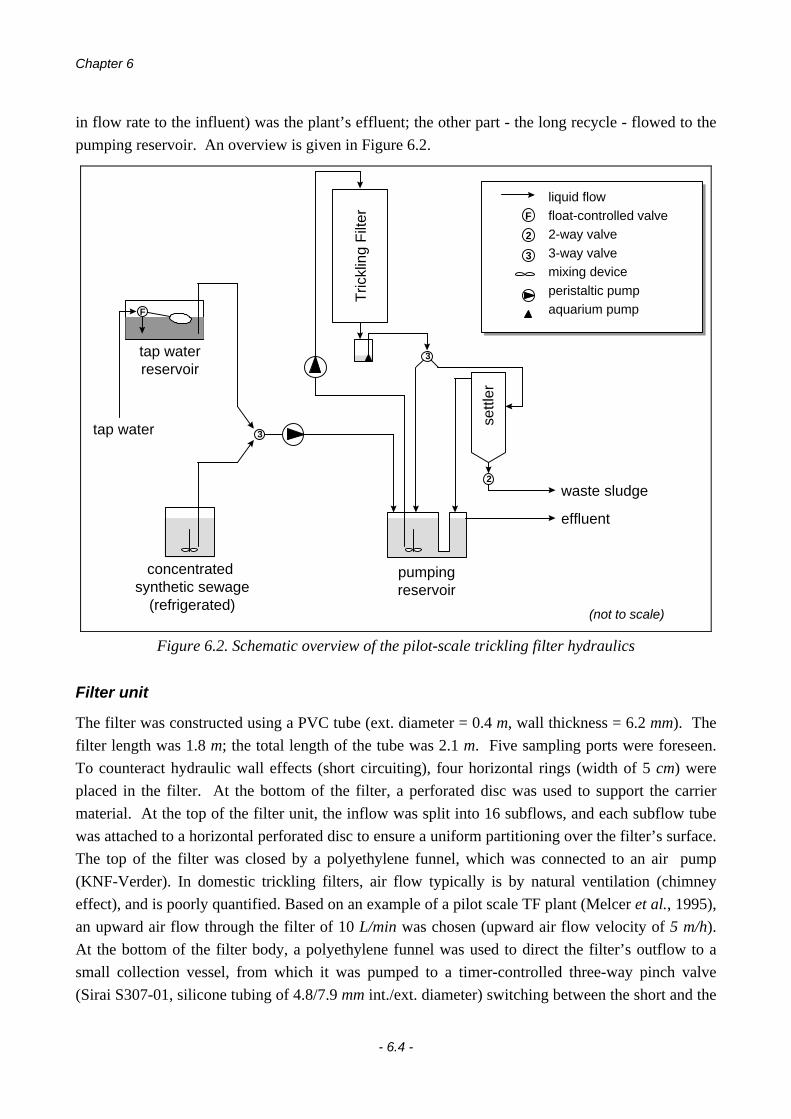
Chapter 6
- 6.4 -
in flow rate to the influent) was the plant’s effluent; the other part - the long recycle - flowed to the
pumping reservoir. An overview is given in Figure 6.2.
tap water
concentrated synthetic sewage
(refrigerated)
effluent
Tric
klin
g F
ilter
settl
erwaste sludge
pumpingreservoir
tap waterreservoir
F
2
3
(not to scale)
3
liquid flowfloat-controlled valve2-way valve3-way valvemixing deviceperistaltic pumpaquarium pump
F
3
2
Figure 6.2. Schematic overview of the pilot-scale trickling filter hydraulics
Filter unit
The filter was constructed using a PVC tube (ext. diameter = 0.4 m, wall thickness = 6.2 mm). The
filter length was 1.8 m; the total length of the tube was 2.1 m. Five sampling ports were foreseen.
To counteract hydraulic wall effects (short circuiting), four horizontal rings (width of 5 cm) were
placed in the filter. At the bottom of the filter, a perforated disc was used to support the carrier
material. At the top of the filter unit, the inflow was split into 16 subflows, and each subflow tube
was attached to a horizontal perforated disc to ensure a uniform partitioning over the filter’s surface.
The top of the filter was closed by a polyethylene funnel, which was connected to an air pump
(KNF-Verder). In domestic trickling filters, air flow typically is by natural ventilation (chimney
effect), and is poorly quantified. Based on an example of a pilot scale TF plant (Melcer et al., 1995),
an upward air flow through the filter of 10 L/min was chosen (upward air flow velocity of 5 m/h).
At the bottom of the filter body, a polyethylene funnel was used to direct the filter’s outflow to a
small collection vessel, from which it was pumped to a timer-controlled three-way pinch valve
(Sirai S307-01, silicone tubing of 4.8/7.9 mm int./ext. diameter) switching between the short and the

Measuring the Fate of LAS in a Pilot-Scale Trickling Filter
- 6.5 -
long recycle (by means of an aquarium pump: Rena C40 Turbo, max. capacity 1000 L/h). By an
electronic balance (modified Mettler-Toledo Spider 1S-150, max. capacity 150 kg, accuracy 10 g)
connected to a PC, the filter unit’s mass was continuously monitored. This information could be
used to determine hydraulic and biofilm characteristics. A schematic overview of the filter unit is
shown in Figure 6.3.
40 cm
36 cm
ring
perforated disc
carrier material180 cm
off-gas
influent
air inflow
effluent
balance
influent partitioningsystem
sampling port
Figure 6.3. Schematic drawing of the pilot-scale trickling filter body
Settler
The settler was constructed from transparent plexi-glass. The settler was located below the filter
unit, but hydraulic headlosses in the tubing made gravitational flow unreliable. Hence, a small
pump was required (see higher). The waste sludge flow was periodically switched on by means of a
timer-controlled two-way pinch valve (Sirai S106-03, with silicone tubing of 6.4/9.5 mminternal/external diameter).

Chapter 6
- 6.6 -
Pumping Reservoir
The influent and the short recycle flows were mixed in the pumping reservoir. Through hydraulic
contact with the effluent reservoir (which received the settler’s outflow), the long recycle flow could
also enter the pumping reservoir. To avoid settling of solids, the pumping reservoir was
continuously mixed by means of a small aquarium pump (Rena C10, max. capacity 240 L/h).
Influent
As influent to the trickling filter plant, a synthetic sewage was used which aimed to mimic real
domestic waste water. A synthetic medium was preferred over actual sewage, because (1) its
composition is constant; (2) its composition is well-characterized; (3) its composition can be
controlled; and (4) for practical reasons: a synthetic sewage can be prepared as a concentrate which
is only to be diluted when it enters the plant. The composition of the sewage was based on the
Syntho medium (Boeije et al., 1998a) which is also described in chapter 4 of this thesis. For cost
reduction, this medium was slightly simplified: urea: 55, NH4Cl: 13 Na-acetate.3H2O: 148, peptone:
17, MgHPO4.3H2O: 29, K3PO4: 20, CaCl2: 2.3, FeSO4.7H2O: 5.8, NaHCO3: 29, starch: 122, milk
powder: 116, yeast: 52, soy oil: 29, Na-LAS paste (60%): 14, Alkyl Ethoxylate (Neodol) (100%): 9,
Cr(NO3)3.9H2O: 0.770, CuCl2.2H2O: 0.536, MnSO4.H2O: 0.108, NiSO4.6H2O: 0.336, PbCl2: 0.100,
ZnCl2: 0.208 (in mg/L). The calculated COD:N:P ratio of the synthetic sewage is 462:43:9 or
100:9.3:2. The theoretical BOD (assuming a COD to BOD conversion factor of 0.65) is 300 mg/L.
In practice, the influent was prepared as a concentrated liquid (20x or 30x), and was diluted with tap
water when it was pumped into the filter setup. One pump was used for this purpose, which
alternated between concentrate and tap water by means of a timer-controlled three-way pinch valve
(Sirai S307-01, with silicone tubing of 4.8/7.9 mm internal/external diameter) (time intervals for
20x concentrated influent: 2 seconds / 38 seconds). A constant supply of tap water was provided in
a reservoir which was continuously filled by means of a float-controlled valve (cf. toilet system).
To keep its quality constant, the concentrated sewage was stored in a refrigerator, and was
continuously mixed by means of 2 aquarium pumps (Rena C40 Turbo, 1000 L/h).
2.2. Hydraulic Characterization
2.2.1. Without Biofilm
A NaCl tracer test was conducted on the filter without biofilm (i.e., before the startup of the
biological experiments). NaCl was injected into the filter as a pulse, and subsequently the NaCl was
detected in the filter’s outflow using conductivity measurements (Yokogawa sensor). The filter was
operated ‘single-pass’ (no effluent recycle was applied). After the injection of the tracer, pure tap
water was pumped over the filter. The test was conducted with two flow rates (1.66 and 0.81
L/min). Based on the tracer response, the mean and mode tracer residence times (TRT) were

Measuring the Fate of LAS in a Pilot-Scale Trickling Filter
- 6.7 -
obtained (Table 6.2). For a flow of 1.3 L/min, linear interpolation resulted in an estimated mean and
mode TRT of 6.35 and 1.89 minutes.
The tracer response curves are presented in Figure 6.4. Note that the raw conductivity data (in
mS/cm) were transformed to E-curves (for which the surface under the curve equals 1).
0.81 L/min
0
0.05
0.1
0.15
0.2
0.25
0.3
0 10 20 30 40 50 60
Time (min)
1.66 L/min
0
0.1
0.2
0.3
0.4
0.5
0.6
0 10 20 30 40 50 60
Model
Data
Figure 6.4. Tracer test without biofilm (E-curves)
The open vessel advection-dispersion model (Levenspiel, 1972) was fitted to the experimental tracer
data (v and D fitted, l fixed at 1.8 m):
( )E
v
D t
l v tD t
=⋅ ⋅
⋅ −− ⋅⋅ ⋅
4 4
2
πexp [6.1]
The fitted parameter values (sum of squared errors (SSE) minimization, SPSS software, version 7.5,
SPSS Inc.) are given in Table 6.2. Although the determination coefficients R2 indicate an acceptable
fit, Figure 6.4 shows that the measured tracer response was heavier in the tail region compared to
the model, and the model also underpredicted the importance of the mode.
Table 6.2. Tracer test without biofilm - results
0.81 L/min 1.66 L/min
from tracer data
TRT mean (min) 8.75 3.28
TRT mode (min) 2.42 1.50
from advection-dispersion model fitting
v (m/s) 0.009491 0.017159
D (m2/s) 0.002533 0.003685
R2 (-) 0.9075 0.9676

Chapter 6
- 6.8 -
2.2.2. With Biofilm
As high NaCl concentrations may disrupt biological activity, the fluorescent agent Thioflavine-S
was used as a tracer when biofilm was present. This tracer was injected into the filter as a pulse,
and its fluorescence was measured in the filter’s outflow (Ingold fluorescence detector, excitation
wavelength 360 nm, measurement wavelength 450 nm). The filter was operated ‘single-pass’.
After the tracer injection, tap water was pumped over the filter. The test was conducted with 3 flow
rates (0.42, 0.83 and 1.3 L/min). The tracer response (E-curves) is shown in Figure 6.5.
1.3 L/min
0
0.0050.01
0.0150.02
0.0250.03
0.0350.04
0.0450.05
0 50 100 150
0.83 L/min
0
0.005
0.01
0.015
0.02
0.025
0.03
0.035
0 50 100 150
0.42 L/min
0
0.002
0.004
0.006
0.008
0.01
0.012
0.014
0.016
0.018
0 50 100 150
Time (min) Model
Data
Figure 6.5. Tracer test with biofilm (E-curves)
As the tails were especially heavy, the tracer experiments could not be conducted until complete
disappearance of the tracer. To complete the curves, a tail extrapolation was performed. The mean
and mode TRTs are given in Table 6.3.
Table 6.3. Tracer test with biofilm - results
0.42 L/min 0.83 L/min 1.3 L/min
from tracer data
TRT mean (min) 84.0 40.0 38.6
TRT mode (min) 7.8 5.1 3.7
from advection-dispersion model fitting
u (m/s) 0.001312 0.002288 0.003207
D (m2/s) 0.002319 0.003179 0.004682
R2 (-) 0.9330 0.9150 0.8947

Measuring the Fate of LAS in a Pilot-Scale Trickling Filter
- 6.9 -
The advection-dispersion model was fitted to the experimental tracer data (Table 6.3) (SSE
minimization, SPSS software, version 7.5, SPSS Inc.). The quality of the fit was similar to that in
the ‘no biofilm’ case. As for the tracer test without biofilm, the measured tracer response data were
heavier in the tail region compared to the model, and the model also underpredicted the importance
of the mode TRT (Figure 6.5). However, the large discrepancy between the modeled and real tracer
tail is not fully reflected in the R2 values, as the measurements used to fit model were not continued
until complete disappearance of the tracer. Hence, it is expected that the presented coefficients of
determination are too optimistic.
2.2.3. Amount of water in the filter
The mass of the filter unit was monitored on-line. The dry mass was determined prior to the
experiments: 62.93 kg. The total mass of water present in the filter (in the absence of biofilm) was
measured at a filter inflow rate of 1.3 L/min: 6.66 kg. At this flow, the ‘dynamic’ amount of water
present in the filter was measured by stopping the inflow: 1.45 kg. Hence, the ‘static’ amount of
water (which remains in the filter even if there is no inflow) was found to be 5.21 kg.
In the presence of biofilm, the ‘dynamic’ water layer mass was 3.06 kg with a flow of 1.3 L/min and
2.38 kg at 0.5 L/min. Assuming that the ‘static’ water mass was not affected by the presence of
biofilm or by the flow, the total water mass in the presence of biofilm was 8.27 kg (at 1.3 L/min)
and 7.59 kg (at 0.5 L/min). From this information, the mean hydraulic residence time in the
presence of biofilm was estimated to be 6.36 min (with a flow of 1.3 L/min) or 15.18 min (at 0.5
L/min). In the absence of biofilm, this was estimated to be 5.12 min at a flow of 1.3 L/min. Based
on the water volume, the total filter volume (213 L) and the porosity (96 %), the fraction of water in
the filter pores (in the presence of biofilm) was calculated to be 4 % at 1.3 L/min and 3.7 % at 0.5
L/min.
2.2.4. Discussion
As expected, in all examined cases the hydraulic residence time in the filter was inversely
proportional to the water flow rate. It was not possible to perfectly describe the tracer response by
means of the open vessel advection-dispersion model: the model underpredicted the importance of
the tail (especially in the presence of biofilm) and of the peak height. Still, the coefficients of
determination indicated an acceptable fit (R2 around 90 % or higher).
A large difference between the mean tracer residence time in the case with and without biofilm was
detected. With a flow of 0.8 ; 1.3 L/min, this was by a factor 4.6 ; 6.1. For the mode (peak), the
difference was more limited (a factor 1.3 ; 2.0).
For 1.3 L/min, the mean TRT in the absence of biofilm deviated less than 25 % from the HRTestimated from the mass of water present in the filter. In the presence of biofilm, this deviation was
more than 600 %. The tracer residence time in the presence of biofilm is expected to be an
overestimation of the hydraulic residence time. The heavy tails of the E-curves can be explained by

Chapter 6
- 6.10 -
diffusion of the tracer substance into the biofilm, later followed by diffusion back into the water
phase (e.g. Rozzi & Massone, 1995). Because of this, the tracer retention in the filter is expected to
be much longer than the hydraulic retention as such. This explains the discrepancy between the
HRT estimated from the amount of water in the filter and the measured TRT in the presence of
biofilm.
2.3. Biofilm and Suspended Solids Characterization
2.3.1. Biofilm Density
Biofilm density was determined by measuring the dry weight (24 hours at 100 °C) of a known
volume (2 mL) of biofilm, which was scraped off the trickling filter’s carriers. Three replicates
were performed, for which the biofilm was sampled from three different carriers, taken from
different locations in the filter. The biofilm density was found to be 38.8 ± 0.8 g/L. This
corresponds well with the typical value of 40 g/L which is e.g. mentioned in Melcer et al. (1995).
2.3.2. Biofilm Thickness
Total biofilm thickness was determined using two different methods: (1) based on the wet and dry
biofilm mass attached to individual carriers, and (2) based on the mass of the entire filter unit.
Based on mass of individual carriers
The wet biofilm mass attached to one carrier was calculated as the difference of the wet (but leaked
out) mass of a carrier taken out of the filter, and the dry mass of a ‘clean’ carrier. The associated
dry biofilm mass is obtained as the difference of the dried mass (24 hours at 100 °C) of the carrier,
and the dry mass of a ‘clean’ carrier. The wet biofilm volume was derived from its wet mass by
assuming a density of 1 kg/L. The dry biofilm mass was calculated back to wet biofilm volume by
means of the measured biofilm density of 38.8 g/L (see above). Biofilm thickness was obtained by
dividing the wet biofilm volume by the surface area of one carrier material (Table 6.4).
Table 6.4. Total biofilm thickness based on mass of individual carriers
May 18 June 11
Based on wet biofilm mass 430 ± 64 µm 526 ± 205 µm
Based on dry biofilm mass 428 ± 86 µm 687 ± 354 µm
Number of measurements 4 3

Measuring the Fate of LAS in a Pilot-Scale Trickling Filter
- 6.11 -
Based on the entire filter unit mass
The wet biofilm mass present in the filter could be determined by subtracting the total (static +
dynamic) water mass and the dry filter mass (see higher) from the total filter mass. This was
converted to volume using a density of 1 kg/L. By dividing this volume by the total carrier surface
area within the filter (46.86 m2), an average biofilm thickness (over the entire filter) was obtained.
The on-line mass measurements during the experiments, together with the calculated biofilm
thickness, are illustrated in Figure 6.6. During the first month of operation, the calculated biofilm
thickness evolved from 50 to 100 µm. The next month it quickly evolved to more than 900 µm.
Because of the balance’s limited capacity, it was necessary to reduce the filter’s mass by feeding
with only tap water for 1 week. This reduced biofilm thickness, which varied between 500 and 750
µm during the next 2 months. The average calculated biofilm thickness over the entire period was
410 (± 260) µm.
0
20
40
60
80
100
120
1-Apr 16-Apr 1-May 16-May 31-May 15-Jun 30-Jun 15-Jul 30-Jul
Date
To
tal f
ilter
mas
s (k
g)
0
100
200
300
400
500
600
700
800
900
1000
Cal
cula
ted
bio
film
th
ickn
ess
(µm
)total filter mass (kg)
biofilm thickness (µm)
Figure 6.6. Filter mass and calculated total biofilm thickness
Interpretation and discussion
The average total biofilm thickness measurements obtained using the different presented methods
are in the same order of magnitude, which shows the reliability of the on-line results.
In biofilm modeling after Melcer et al. (1995), the active biofilm thickness is required rather than
the total thickness. In the case of LAS biodegradation, presence of oxygen is needed for activity
(e.g. Jimenez et al., 1991). However, it may be that only the upper layer of a biofilm is aerobic (e.g.
Horn & Hempel, 1997). In the measurements presented here, the total biofilm thickness was
determined, thus including both active and inactive biomass. Hence, these measurements can not be
used as such to describe the active biofilm thickness.
Chapter 6
- 6.12 -
Ramsing et al. (1993) analyzed the O2 profiles in a 4500 µm thick trickling filter biofilm. They
found a maximal O2 penetration depth of 400 µm; O2 levels dropped below 1 mg/L at a depth of 200
µm. This biofilm was incubated using a medium with a COD of 90 mg/L. In the trickling filter
described in this chapter, the biofilm was in contact with higher COD levels (between ∼200 mg/L at
the filter’s top and ∼100 mg/L at its bottom) which are expected to have caused a faster O2 depletion
in the biofilm, and hence a lower penetration depth. In Verstraete (1992), it is mentioned that - in
general - a biofilm using organics is only functional to a depth of 50 - 100 µm. In a calculation
example for a trickling filter, Henze et al. (1995) derived an O2 penetration depth of 117 µm.
Based on these different considerations, it is a realistic assumption that from May onwards, the
biofilm thickness which was active in LAS degradation was in the order of 100-200 µm.
2.3.3. Suspended Solids
Suspended solids were determined in the influent, the pumping reservoir, the filter outflow, and the
final effluent. Duplicate measurements were made at four different dates, resulting in the following
values: influent: 124 ± 51 mg/L, pumping reservoir: 22 ± 14 mg/L, filter outflow: 33 ± 31 mg/L,
effluent: 15 ± 8 mg/L. The variability was especially high for the filter outflow. This is most
probably due to the irregularity of the biomass sloughing process. Based on the SS measurements in
the filter outflow and in the final effluent, a solids removal efficiency in the settler of (36.5 ± 7.5) %
could be calculated.
2.3.4. LAS and COD Removal Experiments
Four different experimental series were conducted. In series (A) and (B), only the short recycle (i.e.,
bypassing the settler) was used. In series (A), the operating conditions were typically high-rate,
while in series (B), conditions were closer to low-rate as the recycle flow was much lower. Series
(C) was conducted to determine the influence of the long recycle (i.e., over the settler). Except for
the recycle regime, it was identical to series (A). In series (D), the influent LAS concentration was
3-4 times higher than in the other experimental series. Due to a malfunctioning valve there was no
short recycle, hence the recycle regime was also different. The experimental conditions in the
different series are given in Table 6.5 below. LAS and COD concentrations were measured at four
locations: (1) influent (total); (2) pumping reservoir (total); (3) filter outflow (total); (4) final
effluent (total + dissolved). The average total biofilm thickness is also given in Table 6.5. As
mentioned higher, the active biofilm thickness was expected to be lower (100-200 µm in all series).

Measuring the Fate of LAS in a Pilot-Scale Trickling Filter
- 6.13 -
Table 6.5. Experimental conditions in the pilot-scale trickling filter(for LAS and COD removal experiments)
Series A Series B Series C Series D
Date (from - to) 28-Apr
28-May
28-May
4-Jun
11-Jun
2-Jul
2-Jul
3-Aug
Influent flow rate (mL/min) 290 290 290 290
Recycle ratio (-) 3.5 0.5 3.5 3.5
- Short recycle ratio (-) 3.5 0.5 1.75 0
- Long recycle ratio (-) 0 0 1.75 3.5
Influent COD (mg/L) (measured) 414 360 ± 8 397 ± 94 387 ± 17
Influent LAS (mg/L) (measured) 5.3 ± 2.1 3.5 ± 0.5 4.2 ± 0.9 15.2 ± 4.5
Total biofilm thickness (µm) 100 - 500 500 - 700 500 - 700 550 - 750
3. Analytical Methods
LAS was measured by means of an aspecific analytical method for anionic surfactants based on the
Azure-A dye reaction, after Den Tonkelaar & Bergshoeff (1969). This method was applicable
because no other anionic surfactants than LAS were present in the filter’s synthetic influent. The
LAS samples were preserved by adding 3% formaline solution (1% formaldehyde). COD was
determined by means of Dr. Lange test kits (Dr. Bruno Lange GmbH). Dissolved effluent samples
were obtained after filtration using an Schleicher & Schuell filter (S&S 597½). Suspended solids
were determined after Standard Methods (APHA et al., 1995).
4. Results & Discussion
4.1. Trickling Filter - LAS and COD Removal Experiments
4.1.1. Results
An overview of the LAS measurements and removal efficiencies is given in Table 6.6. The
measurements in the pumping reservoir were considered unreliable, as sampling (in this vessel as
well as at all other locations) disrupted the hydraulic balance in this tank. Instead, concentrations
for the pumping vessel were calculated from the mass balance of the measured concentrations in the
influent and the recycle flows (assuming complete mixing of these flows). To derive the single
pass LAS removal in the filter unit as such (i.e., filter outflow vs. pumping reservoir), these
calculated concentrations were used.
The average COD removal efficiency which was measured in the trickling filter was 85 ± 6 %, with
no significant difference between the different experimental series (Tukey test, α = 0.05).

Chapter 6
- 6.14 -
On average, LAS removal in the settler (i.e., between final effluent and filter unit’s outflow) was
negligible. The average calculated removal was close to zero, sometimes negative, and variability
was very high. For COD, the average removal over the settler was (16 ± 21) %. The high
variability can be explained by the poor settling properties of the filter’s sludge, and by the very
irregular sloughing behavior.
By means of a Tukey test (α = 0.05) (SPSS software version 7.5, SPSS Inc.), no statistically
significant difference was found between LAS removal in the first three experimental series.
However, removal in Series D (with higher influent LAS levels) was significantly higher than in the
other series. A Tukey test (α = 0.05) for LAS effluent levels showed no significant difference
between the LAS effluent concentration in all four experimental series.
Table 6.6. Overview of LAS measurements and removals in the pilot-scale trickling filter
Series A Series B Series C Series DShort Recycle Short Recycle,
Low rec. ratioShort + Long
RecycleLong Recycle
High LAS conc.
LAS influent (mg/L) 5.3 ± 2.1 3.5 ± 0.5 4.2 ± 0.9 15.2 ± 4.5
# measurements 9 4 7 5
LAS measurements (% relative to influent concentrations)
Influent (total) 100 100 100 100
Pumping reservoir
- measured (total) 74 ± 20 77 ± 20 61 ± 14 38 ± 14
- calculated (total) 64 ± 17 83 ± 6 56 ± 14 34 ± 8
Filter outflow (total) 54 ± 22 50 ± 17 44 ± 18 15 ± 11
Effluent
- total 51 ± 17 52 ± 24 44 ± 17 15 ± 10
- dissolved 45 ± 16 41 ± 18 36 ± 14 7 ± 5
LAS removal (%)
- complete WWTP 49 ± 17 48 ± 24 56 ± 17 90 ± 3
- single pass * 19 ± 14 41 ± 16 25 ± 15 58 ± 19
* based on calculated concentrations in the pumping reservoir
4.1.2. Discussion
Filter COD removal performance
The COD removal experiments showed that the trickling filter had a normal treatment efficiency.
The measured COD removal of 85 ± 6 % corresponds well with ATV (1985), whose rule of thumb
predicts a treatment efficiency of (93 - 17*BV) % = 82.8 % in this case. There was no significant
effect of the different experimental operating conditions on COD elimination.

Measuring the Fate of LAS in a Pilot-Scale Trickling Filter
- 6.15 -
Comparison of experimental series (LAS removal)
No significant difference in LAS removal was found between the first three experimental series.
When the lower recycle ratio was applied (series B) the single pass removal was much higher than
with the high recycle (series A), but this effect was neutralized by the smaller number of passes
through the filter. Hence, no difference could be seen in the total LAS removal. Applying a long
recycle (series C) next to the short one also had no detectable effect on LAS removal. This can be
explained by the high similarity between the concentrations in the filter outflow and the settler
outflow (both were identical in series C).
There was a clear effect of the influent LAS concentration on the removal efficiency. This effect
was seen in the overall removal efficiency as well as in the single pass removal. LAS effluent levels
in the different experimental series were not significantly different from each other. Hence, the
LAS influent levels did not influence the LAS concentrations in the effluent. This could suggest
that the amount of active biomass, which is capable of biodegrading LAS, may adapt itself to the
higher LAS influent concentrations. Similar observations have been described for activated sludge
by Birch (1991) and by Lee et al. (1998). On the other hand, this effect might also be due to the
occurrence of different kinetics at higher LAS concentrations.
Effect of biofilm thickness
There are a number of reasons to assume that the total biofilm thickness had no effect on LAS
removal. (1) LAS removal in series A, B, and C was not significantly different. On the other hand,
the total biofilm thickness in series B and C was much higher than the biofilm thickness in series A.
(2) In series D, LAS removal was significantly higher than in B and C. However, the biofilm
thickness was similar in these three series. (3) The variability of LAS removal efficiency in series A
(relative standard deviation = 35%) was similar to that in series B (rel. std. dev. = 50%) and C (rel.
std. dev. = 30%). Hence, there was no detectable effect of the 5-fold increase in biofilm thickness
during Series A. On the other hand, the variability in series D was very low (rel. std. dev. = 3%),
even though the variation in biofilm thickness was similar to that found in series B and C.
Based on these considerations, it can be concluded that the active biomass thickness was identical in
all four experimental series. A plausible value for the active biofilm thickness can be estimated as
the minimal total biofilm thickness which occurred: between 100 and 200 µm. This confirms the
considerations mentioned higher in 2.3.2.

Chapter 6
- 6.16 -
5. Conclusions
The removal of LAS in a pilot-scale trickling filter waste water treatment plant was measured as a
function of different operating conditions, and at high and normal LAS influent levels. The effect
of the operating conditions (short versus long recycle, high versus low recycle ratio) was not
significant. At normal LAS influent levels (4 mg/L), LAS removal in this high-rate filter was in the
order of 50 %. On the other hand, a COD removal efficiency between 70 % and 90 % was
monitored. When a 3-4 times higher LAS level was present in the influent (15 mg/L) (with an
unchanged COD concentration), the LAS elimination increased to 90 %.
The higher LAS removal efficiency related to the increased influent concentration may have been
due to biological adaptation to the higher concentrations. On the other hand, it may also indicate a
different kinetic behavior at high concentrations. Further research (preferably dynamic
experiments) is required to study the effect of biological adaptation to different LAS influent
concentrations on removal efficiency.

Chapter 7 -
A Steady-State Non-Equilibrium Chemical FateModel for Trickling Filters
a condensed version of this chapter, together with chapter 6, was submitted for publication as:
Boeije, G., Vanhooren, H. & Vanrolleghem, P.A. (submitted) Development of a steady-statechemical fate model for trickling filters supported by measurements in a pilot-scale plant.Submitted to Environmental Science and Technology.
- 7.1 -
Chapter 7
A Steady-State Non-Equilibrium Chemical FateModel for Trickling Filters
1. Introduction
Over the last 20 years, several models which describe the fate and behavior of individual organic
compounds in biofilms have been formulated (e.g. Harremoës, 1978; Rittmann & McCarty, 1980;
Namkung et al., 1983; Stratton et al., 1983; Namkung & Rittmann, 1986a and 1986b; Golla &
Overcamp, 1990; Melcer et al., 1995). Specific applications to trickling filter systems are given in
e.g. Duncan et al. (1995), Melcer et al. (1995) and Snape et al. (1995). In this chapter, the
development of a chemical fate model for trickling filters is presented, based on the SIMPLEBOXapproach (van de Meent, 1993) combined with the biofilm diffusion / biodegradation model of
Melcer et al. (1995). The SIMPLEBOX approach calculates chemical fate under steady-state non-
equilibrium conditions, using a mass balance between several completely mixed boxes. This
method was also used for activated sludge modeling in SimpleTreat (Struijs et al., 1991b), of which
an adapted version was selected for use within the GREAT-ER project (described in chapter 5 of
this thesis).
The biodegradation and sorption aspects of the newly developed fate model were tested by
experimental data for the surfactant LAS (Linear Alkylbenzene Sulphonate) obtained in a pilot-scale
trickling filter setup (see chapter 6 of this thesis). The model was also applied to predict the fate of
LAS in two full-scale trickling filter plants in Yorkshire (UK), for which a detailed LAS removal
study was performed in the scope of the GREAT-ER project (Holt et al., 1998).
2. Model Formulation
2.1. Process Description
The modeled configuration was limited to the trickling filter process as such, i.e. a filtration unit
coupled with a secondary settler (Figure 7.1). Primary settling was not taken into account. Short
and long effluent recycles were considered (i.e. both before and after the secondary settler). The
secondary settling process in a trickling filter plant is similar to that in activated sludge, the main
difference being that sludge is not recycled.

Chapter 7
- 7.2 -
secondary settler
effluent
waste sludge
trickling filter
trickling filterinfluent
‘long’ recycle water
‘short’ recycle water
Figure 7.1. Trickling filter model - plant configuration
An overview of biological and chemical processes which may occur in a trickling filter is given in
Figure 7.2. Chemicals are present in the dissolved phase and sorbed to suspended solids. Through
ad-/desorption there may be an interchange between these two phases. The dissolved chemical can
diffuse into the biofilm. Suspended solids with sorbed chemicals may be filtered out of the water;
on the other hand chemicals associated with biofilm solids may be released to the water phase in the
sloughing process. (Biological) degradation may take place both inside the biofilm and in the water,
both in the adsorbed and the dissolved phases. Finally, the dissolved chemical may be subject to
volatilization, and be removed with the ventilation air.
wastewater ventilation
air
carrier materialbiofilm
adsorbedchemical
dissolvedchemical diffusion
filtration /sloughing
volatili-zation
ad-/de-sorption
biodegradation
Figure 7.2. Chemical fate processes in a trickling filter (overview)

A Steady-State Non-Equilibrium Chemical Fate Model for Trickling Filters
- 7.3 -
2.2. Systems Analysis and Segmentation
To apply the SIMPLEBOX approach, the trickling filter system was split up into a number of
completely mixed boxes (Figure 7.3). The first segmentation was between the air above the plant,
the filter unit, and the settler. The settler was further divided into a dissolved (water) and a sorbed
(solids) phase. A settled sludge box (cf. SimpleTreat) was not needed, as sludge is not recycled.
The filter itself was split up into several horizontal layers, connected in series (cf. tanks-in-series
model to model imperfect plug flow hydraulics). The actual number of layers is determined by the
hydraulics of the modeled filter unit, by the required accuracy and by the desired computation speed
of the model.
Each horizontal layer of the filter was subdivided into three compartments (Figure 7.3, Figure 7.4):
pore air, pore water (dissolved phase) and pore water (sorbed phase). Downward transport of
chemicals through the filter unit is between the pore water phase of the different layers. By
ventilation, pore air is transported upward between the layers. Within a layer, exchange processes
take place between air and water (volatilization) and between the sorbed and dissolved phases.
Biodegradation mainly occurs by biofilm activity. Continuous chemical diffusion from the pore
water into the biofilm is only possible if a concentration gradient is maintained by biodegradation in
the biofilm. These coupled processes are dealt with by the steady-state biofilm model of Melcer etal. (1995). In this model the calculated diffusion flux from the pore water (dissolved phase) into the
biofilm is expressed as removal out of the water phase. In this approach, the biofilm compartment
need not be represented as an extra box (Figure 7.4). To simplify the model, it was assumed that
filtration and release (by sloughing) of the sorbed chemical balance each other, resulting in a zero
net effect. Furthermore, chemical sorption equilibria within the biofilm were not considered in the
biodegradation model.
Next to the between-layer transport, there is transport of air from the top layer of the filter to the air
above the plant, and volatilization from the settler surface. There is water and solids transport by
means of the long and short effluent recycles to the first filter layer. Influent (dissolved and sorbed
phase) enters the plant into the top filter layer, and effluent (dissolved and sorbed phase) leaves the
plant via the settler, as well as waste sludge (sorbed phase only). Finally, the air above the plant is
refreshed by the wind and ambient air flows counter-current through the filter unit (either by the
chimney effect or by forced aeration).
As the number of layers n used to describe the filter unit is not necessarily fixed, the following
flexible box numbering approach was followed in this text (Figure 7.3). The ‘outside world’ is box
0; the air compartment above the WWTP is box 1. Each horizontal layer i has the box numbers
Li+1 until Li+3 (dissolved, sorbed, air), with Li = 1+3*(i-1). The settler has box numbers S+1 and
S+2 (dissolved, sorbed), with S = 1+3*n.

Chapter 7
- 7.4 -
pore air
Li+3pore water(dissolved)
Li+1
pore water(sorbed)
Li+2
air above WWTPn
laye
rs1
settler water(dissolved)
S+1
settler water(sorbed)
S+2
ambient aireffluent
influent
advective transportdiffusive exchangedegradation waste sludge
Figure 7.3. Entire trickling filter plant: model scheme
carrierbiofilmwaterair
dissolvedchemical
sorption / desorption
gaseouschemical
volatilization
filtering
sloughing
net diffusion
biodegradation
sorbedchemical
Figure 7.4. Processes in one horizontal trickling filter layer: model scheme

A Steady-State Non-Equilibrium Chemical Fate Model for Trickling Filters
- 7.5 -
2.3. Calculations
2.3.1. Influent
The influent (dissolved and sorbed chemical fraction) enters the treatment system simultaneously
into box 2 and box 3. Without a primary settler, the dissolved and sorbed influent fractions are
assumed to be in complete equilibrium:
- into filtration unit (dissolved): Φ Φin intf
sewage dsewageSS K
26
1
1 10= ⋅
+ ⋅ ⋅− [7.1]
- into filtration unit (sorbed): Φ Φin intf sewage d
sewage
sewage dsewage
SS K
SS K3
6
6
10
1 10= ⋅
⋅ ⋅+ ⋅ ⋅
−
− [7.2]
If a primary settler model is connected in front of the trickling filter model, the dissolved/sorbed
fractionation obtained in the former is used to calculate the influent partitioning:
- into filtration unit (dissolved): Φ Φin intf
dprimaryf2 = ⋅ [7.3]
- into filtration unit (sorbed): Φ Φin intf
sprimaryf3 = ⋅ [7.4]
2.3.2. Advective Transport Fluxes
The advective transport between layers is described for a generic layer with number i. Non trickling
filter specific equations were taken from Struijs (1996).
Air advection
- into / out of area above WWTP: ADV ADV h v A Aair wind filter sec0 1 1 0, ,= = ⋅ ⋅ + [7.5]
- air into / out of / between pores: ADV ADV QL L Lair
n i i0 3 3 31, ,+ + += =−
[7.6]
Water volume flow rates
- into / out of WWTP: ADV ADV QL S0 1 1 01, ,+ += = [7.7]
- propagation through filter: ( )ADV Q f fL L rec reci i+ ++= ⋅ + +1 1
1 2
11, [7.8]
- filter to secondary settler: ( )ADV Q fL S recn + + = ⋅ +1 121, [7.9]
- effluent recycles: - before settler: ADV Q fL recn + = ⋅1 21
, [7.10]
- after settler: ADV Q fS rec+ = ⋅1 22
, [7.11]

Chapter 7
- 7.6 -
Solids volume flow rates
In the SIMPLEBOX approach, all flow rates are expressed as volume flows. Hence, solids mass
fluxes were recalculated to volumetric fluxes, using the solids’ density.
- influent into WWTP: ADVSS
Qsewage
solidssewage0 3 610, =
⋅⋅
ρ[7.12]
- propagation through filter: ( )ADVSS
Q f fL Ltf
solidstf rec reci i+ ++
=⋅
⋅ ⋅ + +2 2 61 2
1 101, ρ
[7.13]
- filter to secondary settler: ( )ADVSS
Q fL Stf
solidstf recn + + =
⋅⋅ ⋅ +2 2 6
2
101, ρ
[7.14]
- effluent recycles: - before settler: ADVSS
Q fLtf
solidstf recn + =
⋅⋅ ⋅2 3 6
1
10, ρ[7.15]
- after settler: ( )ADV RSS
Q fS secSS tf
solidstf rec+ = − ⋅
⋅⋅ ⋅2 3 6
2110, ρ
[7.16]
- effluent + waste sludge out of WWTP: ADVSS
QS
tf
solidstf+ =
⋅⋅2 0 610, ρ
[7.17]
2.3.3. Diffusive Exchange
For the calculation of the diffusive exchanges, the fugacity approach is applied. Expressions for
fugacities, diffusion coefficients and kinetics were taken from Struijs (1996), after Mackay and
Paterson (1982).
Fugacities
- air:( )
ZR tair
air
=⋅ +
1
273[7.18]
- water: ZHwater =1
[7.19]
- filter unit solids: ZK
Htfdtf
solidstf
=⋅ ρ
[7.20]
Box volumes
- air above the WWTP: ( )V A A htf sec air1 = + ⋅ [7.21]
- filter unit (water): VV f
nLtf tf water
i +=
⋅ ⋅1
ε ε
[7.22]

A Steady-State Non-Equilibrium Chemical Fate Model for Trickling Filters
- 7.7 -
- filter unit (suspended solids): VV f
n
SSL
tf tf water tf
solidstfi +
=⋅ ⋅
⋅⋅2 610
ερ
ε
[7.23]
- filter unit (air): VV f
nLtf tf air
i +=
⋅ ⋅3
ε ε
[7.24]
- secondary settler (water): V VS sec+ =1 [7.25]
- secondary settler (solids):( )
V VR SS
S sec
secSS
tf
solidstf+ = ⋅
− ⋅
⋅2 6
1
10 ρ[7.26]
The sum of pore fractions f f fwater air biofilmε ε ε+ + = 1. These fractions may depend on the type and size
of carrier material, on the biofilm age, and on hydrodynamic conditions.
Media volume flow rates
D Dk
V Z V Z
i j j idiff
i i j j
, ,= =
⋅+
⋅1 1
[7.27]
Next, the exchange from box i to j (expressed as a volume flow rate) is calculated as:
XCHD
Zi ji j
i,
,= [7.28]
Suspended solids / water exchange
- filter unit:
D Dk
V Z V Z
L L L Ltfsorb
L water L tf
i i i i
i i
+ + + +
+ +
= =
⋅+
⋅
1 2 2 1
1 2
1 1, , [7.29]
→ XCHD
ZL LL L
wateri i
i i
+ ++ +=1 2
1 2,
, XCHD
ZL LL L
tfi i
i i
+ ++ +=2 1
2 1,
,
- secondary settler:
D Dk
V Z V Z
S S S Ssecsorb
S water S tf
+ + + +
+ +
= =
⋅+
⋅
1 2 2 1
1 2
1 1, , [7.30]
→ XCHD
ZS SS S
water+ +
+ +=1 21 2
,, XCH
D
ZS SS S
tf+ +
+ +=2 12 1
,,

Chapter 7
- 7.8 -
The kinetic rates for sorption / desorption are given in Table 5.1 (chapter 5). For trickling filter
solids, the same sorption kinetics were assumed as for activated sludge (after Struijs, 1996).
Air / water exchange
Volatilization was modeled using the two-layer approach (Liss and Slater, 1974; Mackay and
Leinonen, 1975), based on Struijs (1996).
- filter unit:
Surface volatilization was assumed to occur at the air / water interface between pore air and
pore water. It was assumed that the aeration rate (either natural or forced) does not influence
the volatilization process directly (only indirectly by transporting air out of the filter).
Hence, the approach of Mackay et al. (1985) could be used to describe this process.
D DA
K Z K Z
L L L La wL
air air water water
i i i i
i
+ + + += =
⋅+
⋅
3 1 1 3 1 1, ,/ [7.31]
→ XCHD
ZL LL L
airi i
i i
+ ++ +=3 1
3 1,
, XCHD
ZL LL L
wateri i
i i
+ ++ +=1 3
1 3,
,
Aa wLi/ is the interfacial area between pore air and pore water within one horizontal layer of the
trickling filter unit. This can be calculated from the filter’s specific air / water interfacial
area, aa/w.
A aV
na wL
a wtfn
/ /= ⋅
- secondary settler:
For the secondary settler, the expressions for the transfer coefficients Di,j were taken directly
from Struijs (1996), after Mackay et al. (1985).
D DA
K Z K Z
S Ssec
air air water water
1 1 1 1 1 1, ,+ += =
⋅+
⋅
[7.32]
→ XCHD
ZSS
air1 1
1 1,
,+
+= XCHD
ZSS
water+
+=1 11 1
,,
Pore water / biofilm exchange
By diffusion, chemicals are exchanged between the pore water’s dissolved phase and the biofilm.
This process was not described as such, but was considered together with biodegradation as a
lumped chemical elimination from the pore water.

A Steady-State Non-Equilibrium Chemical Fate Model for Trickling Filters
- 7.9 -
2.3.4. Biodegradation
Biodegradation in the dissolved phase of the water compartment consists of biodegradation by
suspended biomass and disappearance of the chemical into the biofilm. This can be expressed as
the sum of two first-order rates. In the sorbed phase of the water compartment, only the suspended
biomass activity is taken into account.
Suspended biomass
“Double” first-order kinetics (both in active biomass and in chemical concentration) can be used to
describe biodegradation. A correction factor can be applied for the sorbed phase, to take into
account the lower bio-availability (e.g. Lee et al., 1998).
k K SSb act= ⋅ [7.33]
Biofilm
Melcer et al. (1995) developed a biofilm model which predicts the mass flux of a chemical
substance from the bulk water phase into the biofilm phase per unit of interfacial area. This process
is driven by diffusion and by biodegradation (which is needed to maintain a concentration gradient
to allow diffusion into the biofilm). An analytical solution for the per area mass flux Nb into the
biofilm is:
( )( )N K
D r r L
D r r L KCb L
e f
e f L
= ⋅⋅ ⋅ ⋅
⋅ ⋅ ⋅ +⋅1 1
1 1
tanh
tanh
rX K
Df b
e1 =
⋅[7.34]
KDLL
l=
The corresponding chemical mass flux calculation to express chemical elimination via degradation
in the SIMPLEBOX approach is:
Φdegradation k C V= − ⋅ ⋅ [7.35]
The flux per unit surface area Nb can be related to the total degradation flux as follows:
NA
k C VAb
degradation=−
=⋅ ⋅Φ
[7.36]
From this, the first-order elimination rate for combined diffusion and biodegradation kbiofilm can be
obtained as:

Chapter 7
- 7.10 -
( )( )k
AV
NC
a KD r r L
D r r L Kbiofilm
bb w L
e f
e f L
= ⋅ = ⋅ ⋅⋅ ⋅ ⋅
⋅ ⋅ ⋅ +/
tanh
tanh
1 1
1 1
[7.37]
Biofilm related parameters
A typical value for the biofilm density Xf is 40 kg/m3 (Melcer et al., 1995). Chemical diffusivity in
the biofilm De can be estimated as a fraction (typically 80 %) of the diffusivity in pure water Dl
(Verstraete, 1992; Melcer et al., 1995). Biofilm thickness Lf is a.o. related to organic loading, to
flow and flow velocity, and to hydraulic shear stress. As estimations of Lf (e.g. Rittmann and
McCarty, 1980 and 1981) require intensive calculations and specific data, this was considered
inappropriate for use in a simple model. As an alternative, a default value for biofilm thickness can
be used. A value in the range of 100-200 µm is appropriate, as substrate and/or oxygen limitation
will typically reduce the active biofilm thickness to this order of magnitude. A default value for the
stagnant water layer thickness L (i.e., the laminar water layer directly in contact with the biofilm) is
100 µm (after Melcer et al., 1995).
In the presented model, the biofilm / water interfacial area has to be known to estimate diffusion
into the biofilm. A biofilm consists of two different structures: a base film, in which the particulate
components form a solid matrix, and a surface film, which has a discontinuous structure (Figure
7.5) (e.g. Wanner & Gujer, 1986; Suschka, 1987; Characklis & Marshall, 1990). It can be assumed
that the surface area of the base film is equal to that of the carrier material. However, the actual
biofilm / water interfacial area is determined by the (higher) surface area of the irregular surface
film. No simple or universal estimation methods for the biofilm / water interfacial area exist. In
this thesis, a correction factor ζbiofilm =2 was used to convert carrier surface to biofilm surface.
air
water
biofilm
carrier (substratum)
base film
surface film
Figure 7.5. Biofilm morphology (schematic)

A Steady-State Non-Equilibrium Chemical Fate Model for Trickling Filters
- 7.11 -
3. Sensitivity Analysis
A sensitivity analysis of the trickling filter model was performed using three hypothetical
substances: the standard SimpleTreat benchmark chemical Hypotheticum (Struijs, 1996), which is
affected by all relevant fate processes in the model (volatilization, sorption and biodegradation), a
Chemical A (volatile), and a Chemical B (sorbing and degradable) (Table 7.1). Contrary to Struijs
(1996), Hypotheticum was assumed to be also degraded in the sorbed phase. For the diffusion
coefficient D an average value from Melcer et al. (1995) was taken. Further, a hypothetical but
realistic trickling filter plant was defined (Table 7.2). The applied environmental conditions and
physical / chemical defaults were taken from Struijs (1996).
Table 7.1. Sensitivity analysis: hypothetical chemical properties
Hypotheticum Chemical A Chemical B
Kdtf (L/kg) 370 10-6 2000
Kdsewage (L/kg) 300 10-6 2000
H (-) 1 100 10-6
Kb ((g/m3)-1.s-1) 9.26 10-9 0 2.78 10-7
αsorbed (-) 0.5 - 0.5Dl (m2/s) 5.55 10-5 5.55 10-5 5.55 10-5
Table 7.2. Sensitivity analysis: plant parameters and default valuesDimensions Flows
Atf 300 m2 Q 0.017361 m3/sVtf 1125 m3
f rec1 0 -
Asec 62.5 m2f rec
2 1 -
Vsec 125 m3 Qair 1.7 m3/sBiofilm and Carrier Suspended Solids
ε 0.5 - SStf 200 g/m3
fwater 0.05 - SSsewage 200 g/m3
fair 0.90 - RsecSS 0.95 -
aa/w 100 m2/m3
ab/w 200 m2/m3
L 10-4 mLf 1.5 10-4 mXf 40000 g/m3
Default Valueshair 10 m ktf
sorb 1.925 10-3 s-1
vwind 1 m/s ksecsorb 1.925 10-4 s-1
ρsolidstf 1.4 kg/L Kair 2.78 10-3 m/s
ρsolidssewage 1.4 kg/L Kwater 2.78 10-5 m/s
tair 20 °C

Chapter 7
- 7.12 -
Sensitivities were calculated for all parameters, for the three test substances. The number of layers
n was fixed at 5. Relative sensitivities were obtained numerically, by increasing the value of each
parameter with 1%, and then applying the following calculation:
SR
RP
P
RRP
P
RRR = =
⋅= ⋅
∆
∆
∆∆
*
*
*
* *
*.0 01100 [7.38]
Note that in this analysis, the effluent recycle was always after the settler (i.e. only long recycle: f rec1
= 0). The resulting relative sensitivities are shown below in Table 7.3. On average, the highest
sensitivities were found for RsecSS (solids removal in the settler), Q (influent flow), SStf (suspended
solids in the trickling filter water phase), Kdtf (chemical sorption equilibrium constant), Vtf (filter unit
volume), ε (carrier material’s porosity), fwater (fraction of water in the filter pores) and Kb (chemical
biodegradation rate constant).
It is stressed that this is a local linear sensitivity analysis of a non-linear model. Because the local
analysis was conducted at three different points (3 completely different chemicals), a tentative
interpretation could be made about which parameters are generally most sensitive and which are
not. A full sensitivity analysis, on the other hand, was outside the scope of this work.
Chemical specific interpretation
The most sensitive parameters for Hypotheticum are related to sorption and settling, volatilization
and (via the hydraulics) to biological contact time. This could be expected as the chemical
undergoes the three associated elimination processes. For Chemical A, the most sensitive
parameters all have an impact on volatilization, as this is the only active fate process. Note that for
this substance, no parameters have a relative sensitivity higher than 5 %, and only 4 parameters have
a sensitivity above 1 %. The removal prediction of Chemical B was mainly influenced by
parameters related to biodegradation and sorption / settling. This was again expected as Chemical
B is highly sorbing and degradable.
Implications for data collection
Except for the diffusion coefficient Dl and the sorbed phase biodegradation correction, all chemical
properties may have high sensitivities, depending on the nature of the chemical. Hence the accuracy
of these (relevant) parameters should be maximized. Dl has a very low sensitivity (rounded to 0% in
all three examined cases); using a default value for this parameter will not significantly affect the
model’s output.
The only important treatment plant dimension is the volume of the filter unit. The flow Q is always
very important; the recycle ratio somewhat less. The air flow Qair only has a high sensitivity for
volatile chemicals.
A Steady-State Non-Equilibrium Chemical Fate Model for Trickling Filters
- 7.13 -
The porosity and the water fraction in the pores had a high sensitivity for 2 substances, while the
fraction of air in the pores had no importance. The interfacial areas air/water and biofilm/water are
important if this interface is limiting for mass transfer or biodegradation - hence, this is chemical-
dependent. The biofilm-related parameters Lf and Xf are sensitive ones for biodegradable
compounds. The stagnant water layer thickness L always has a low sensitivity. The parameters
related to suspended solids and settling are sensitive for highly sorbing chemicals. SSsewage has a
much lower importance than SStf.
Most of the default values have a low sensitivity in all cases. However, the sorption kinetics
constant in the trickling filter ktfsorb is important for sorbing chemicals, and the mass transfer
coefficients Kair and Kwater may be important for volatile substances.

Chapter 7
- 7.14 -
Table 7.3. Sensitivity analysis: relative sensitivities to trickling filter model parameters
Parameter SR (%)Hypotheticum Chemical A Chemical B Average
Chemical Properties
Kdtf 47 0 17.1 22
Kdsewage 6.7 0 3.3 3.3
H 22 3.7 0 8.5Kb 10 0 24 11.5
αsorbed 0.02 0 0.32 0.11Dl 0 0 0 0
Plant Parameters
Atf 0.01 0 0 0Vtf 20 0.31 25 15.2
Asec 1.88 0.03 0 0.64Vsec 0.28 0 -0.04 0.08
Q -42 -4.4 -25 -24f rec
2 17.9 -1.53 6.6 7.7
Qair 20 3.7 0 7.9ε 20 0 25 15.1
fwater 20 0 25 15.1fair 0 0 0 0
aa/w 0.01 0.31 0 0.11ab/w 8.6 0 21 9.7
L 0 0 0 0Lf 8.6 0 21 9.7Xf 8.6 0 21 9.7
SStf 49 0 21 23SSsewage 6.7 0 3.3 3.3
RsecSS 48 0 35 28
hair 0.02 0.01 0 0.01Default Values
vwind 0.02 0.01 0 0.01ρsolids
tf 0 0 0 0
ρsolidssewage 0 0 0 0
tair -1.49 -0.26 0 -0.58ktf
sorb 10.2 0 0.76 3.7
ksecsorb 0.28 0 -0.04 0.08
Kair 1.82 0.07 0 0.63Kwater 0.07 0.27 0 0.12
Notation: SR > 10%, 1% < SR < 10%, SR < 1%

A Steady-State Non-Equilibrium Chemical Fate Model for Trickling Filters
- 7.15 -
4. Model Testing for LAS
The biodegradation and sorption aspects of the presented fate model were tested by applying it to a
pilot-scale trickling filter plant (chapter 6 of this thesis) and to two full-scale plants for which an
LAS monitoring campaign was performed in the framework of the GREAT-ER project (Holt et al.,1998).
The same environmental and default values as in the sensitivity analysis were applied (Table 7.2,
bottom section). Air temperature was approximately 20 °C, both in the lab and in the field study.
The parameters Qair, fair and hair were not required to model the fate of the non-volatile LAS, as they
are only related to volatilization.
The chemical properties used to model LAS are given below in Table 7.4. The Kd (for sewage and
trickling filter solids) and H coefficients were taken from Cowan et al. (1993b). For the value of Dl,an average from Melcer et al. (1995) was taken (not specifically for LAS), as the sensitivity for this
parameter is very low. The sorbed phase biodegradation correction factor αsorbed was set to 1 (cf.
Cowan et al., 1993b; Boeije et al., 1998b).
The double first-order biodegradation rate coefficient (Kb) of LAS was calculated from the first-
order rate coefficient typically used for biodegradation by suspended biomass in activated sludge (3
h-1, with mixed liquor SS = 3000 gdwt/m3) (e.g. Struijs et al., 1991b).
Table 7.4. LAS chemical properties
Kd 2000 L/kg
H 1 * 10-6 Pa.m3.mol-1
Kb 0.278 * 10-6 (g/m3)-1.s-1
αsorbed 1 (-)
Dl 55 * 10-6 m2/s
4.1. Pilot-scale Trickling Filter
Trickling filter plant
LAS removal measurements in a pilot-scale trickling filter plant (chapter 6 of this thesis) were used
to test the presented fate model. Plant operating parameters were known; hydraulics and biofilm
characteristics were measured or estimated (Table 7.5). Four experimental series were conducted,
with different recycles (Table 7.5) and with a normal (4 mg/L) (series A, B and C) versus high (15
mg/L) LAS influent level (series D).
With a total flow of 1.3 L/min (series A, C and D), the HRT for a single pass through the filter was
estimated to be 6.4 minutes (estimated fwater = 4 %). At 0.5 L/min (∼ series B), the estimated HRTwas 15.2 minutes (estimated fwater = 3.7 %) (see also chapter 6 of this thesis).

Chapter 7
- 7.16 -
Measured LAS elimination efficiencies, both ‘single-pass’ and total, are given in Table 7.6 (see also
chapter 6 of this thesis).
Table 7.5. Pilot-scale TF plant - model parameters
Known
Atf (m2) 0.118
Vtf (m3) 0.213
Asec (m2) 0.049
Vsec (m3) 0.034
Q (m3/s) 4.83 10-6
f rec1 , f rec
2 (-) Series A: 3.5, 0
Series B: 0.5, 0
Series C: 1.75, 1.75
Series D: 0, 3.5
εtf - 96 %
Measured
SStf (mg/L) 27.5
SSsewage (mg/L) 124
RsecSS (-) 36.5 %
Xf (g/m3) 38800
Estimated
aa/w (m2/m3) 100
ab/w (m2/m3) 200
Lf (m) 0.000150
Default
L (m) 0.000100
Table 7.6. Pilot-scale TF plant - measured LAS removal efficiencies
Series Total removal (%) Single-pass removal (%)
A 49 ± 17 19 ± 14
B 48 ± 24 41 ± 16
C 56 ± 17 25 ± 15
D 90 ± 3 58 ± 19

A Steady-State Non-Equilibrium Chemical Fate Model for Trickling Filters
- 7.17 -
Model testing
As all required model parameters were known, it was possible to apply the model to the pilot-scale
trickling filter without any calibration based on the measured LAS elimination data. The resulting
total and single-pass removal predictions for the 4 experimental series, next to their relative
deviation from the measurements, are given in Table 7.7.
Table 7.7. Pilot-scale TF plant - uncalibrated predictions for LAS
Series Total removal Single-pass removal
Predicted Relative deviation Predicted Relative deviation
A 55.2 % + 12.6 % 20.4 % + 7.5 %
B 57.2 % + 19.1 % 45.7 % + 11.5 %
C 57.0 % + 1.8 % 20.8 % - 17.0 %
D 58.3 % - 35.2 % 21.0 % - 63.8 %
Next to the uncalibrated simulations, the single-pass removal predictions for the different
experimental series were fitted to the measurements by tuning the parameter related to the amount
of water in the filter (fwater). For series D, with a higher LAS influent concentration, the calibration
of series C was used next to the calibration of fwater and a calibration of Kb. The calibrated fwater
values (together with the corresponding HRT) are given in Table 7.8, next to the predicted total
removal efficiencies and the relative deviation from the measurements.
Table 7.8. Pilot-scale TF plant - model calibration for LAS
Calibration Total removal
fwater (-) HRT (min) Predicted Relative deviation
Series A 3.7 % 5.8 53.0 % + 8.1 %
Series B 3.2 % 15.0 52.6 % + 9.6 %
Series C 5.0 % 7.8 62.3 % + 11.2 %
Series D (1) 15.8 % 24.8 86.8 % - 3.6 %
Series D (2) 5.0 % 7.8 63.3 % - 29.6 %
Series D (3) 5.0 % 7.8 87.6 % - 2.7 %
(1) calibrated fwater
(2) using the fwater calibration of series C (predicted single-pass removal = 25.1 %)
(3) calibrated Kb = 0.991 10-6 (g/m3)-1.s-1 - fwater from series C
Discussion
The uncalibrated predictions for series A, B and C were within one standard deviation of the
measurements’ means, both for total and single-pass removal. The relative deviation from the
means was at the most 20 %. For series D, however, a much larger deviation was found: over 30 %
underestimation for the total removal and over 60 % underestimation for the single-pass.
Chapter 7
- 7.18 -
The calibrated fwater values for series A, B and C are in line with the measured values. Similarly, the
corresponding HRTs in series A, B and C correspond very well with the measured HRTs. The
calibrated fwater for series D and the corresponding HRT are unrealistic: they are a factor 3 higher
than what was expected based on the measurements and on the other series’ calibrations.
Alternatively, the fwater value from the calibration of series C was applied to series D, because both
experimental series were conducted close to each other and were hydraulically very similar.
However, this caused an underprediction of the single-pass removal in series D by 56 %, and of the
total removal by 28 %. To fit the model to series D using realistic hydraulics and biofilm
parameters (which were similar to the other experimental series, see chapter 6 of this thesis), it was
necessary to modify the biodegradation constant Kb. To calibrate the single-pass removal, a Kb of
0.0035 (g/m3)-1.h-1 or 0.979 10-6 (g/m3)-1.s-1 was required, which is 3.5 times higher than the Kb used
for the other experimental series (derived from activated sludge data). This observation indicates
that LAS removal kinetics may be different at higher influent concentrations (possibly because of
adaptation of the competent biomass to these higher concentrations).
The model calibration focused on fitting the predicted single-pass removal to the data. This resulted
in an overprediction of total removal by ca. 10 % in series A, B and C, and in a small
underestimation of total removal in series D (by ca. 3 %). Except for possible inaccuracies in the
measurements of both total and single-pass removal, no other plausible explanation for this
phenomenon could be found.
4.2. Full-scale Sewage Treatment Plants
Trickling filter plants
In the sewage treatment plants of Gargrave and Dowley Gap (Yorkshire, UK), LAS removal over
the trickling filter as such (including secondary settling but excluding primary treatment) was
measured by Holt et al. (1998). Gargrave is a very small plant, treating the sewage of 1450 people,
while the Dowley Gap plant serves a community of 30150 people. For the latter, the volumetric
organic loading BV was 0.07 kgBOD/m3.d (very low loading according to the range given in Metcalf
& Eddy, 1991). BOD removal in this plant was on average 91 %.
Measured flow data and LAS elimination percentages in both treatment plants are given in Table
7.9. Plant dimensions are given in Table 7.10. In these systems, no effluent recycles were applied.
Data on suspended solids were not available; a default value of 200 mg/L (for SStf and SSsewage) was
assumed, together with a secondary settler solids removal efficiency of 90 %. The applied biofilm
and carrier material related data are given in the bottom section of Table 7.10. For both plants, the
bed material consisted of lava rock, with a specific surface area of 100 m2/m3 and a porosity of 50
%. The air/water interfacial area was assumed equal to the carrier material’s specific surface area,
while the biofilm/water area was assumed to be twice that area (i.e. ζbiofilm =2). For the stagnant

A Steady-State Non-Equilibrium Chemical Fate Model for Trickling Filters
- 7.19 -
water zone thickness and the biofilm density, defaults from Melcer et al. (1995) were used. An
active biofilm thickness of 150 µm was selected (cf. considerations in chapter 6).
Table 7.9. Full-scale domestic TF plants - flow data and LAS elimination (August/September ‘96)
Gargrave
Date 19-20 / 8 20-21 / 8 Average
Mean Q (m3/s) 0.0057 0.0078 0.00675
TF influent LAS (mg/L) 2.64 2.28
TF effluent LAS (mg/L) 0.20 0.40
LAS Removal (%) 92.42 82.46 87.44
Dowley Gap
Date 20-21 / 8 21-22 / 8 3-4 / 9 4-5 / 9 Average
Mean Q (m3/s) 0.136 0.104 0.143 0.129 0.128
TF influent LAS (mg/L) 2.60 2.72 1.74 1.69
TF effluent LAS (mg/L) 0.43 0.35 0.35 0.31
LAS Removal (%) 83.46 87.13 79.90 81.66 83.04
Table 7.10. Full-scale domestic TF plants - model parameters
Gargrave Dowley Gap
Known
Atf (m2) 538 13130
Vtf (m3) 1236.5 25130
Asec (m2) 112.5 1016
Vsec (m3) 360 2830
f rec1 , f rec
2 (-) 0 0
Defaults
SStf (mg/L) 200
SSsewage (mg/L) 200
RsecSS (-) 90 %
Biofilm and carrier material
εtf (-) 50 %
aa/w (m2/m3) 100
ab/w (m2/m3) 200
L (m) 0.000100
Lf (m) 0.000150
Xf (g/m3) 40000

Chapter 7
- 7.20 -
Model testing
The parameter fwater was used for calibration. Two calibrations were performed: one based on the
measurements in Gargrave on 19-20 / 8 and one based on the measurements in Dowley Gap on 20-
21 / 8. For Gargrave, the calibrated fwater value was 9.355 %; for Dowley Gap it was 6.552 %. In
both cases, the order of magnitude of the calibrated fwater values was realistic. They corresponded
with a total water layer thickness of 300 - 500 µm and a mean HRT of 5.6 hours in Gargrave or 3.4
hours in Dowley Gap.
Subsequently, these calibrations were applied to all other monitored situations. The predicted and
measured removal efficiencies, as well as the relative deviation of the predictions from the
measurements, is given in Table 7.11.
Table 7.11. Full-scale domestic TF plants - model calibration for LAS
Predicted LAS removal Relative deviation
Calibration based on Gargrave, 19-20 / 8
Gargrave
19-20 / 8 92.4 % calibrated
20-21 / 8 87.4 % + 5.9 %
Dowley Gap
20-21 / 8 90.1 % + 8.0 %
21-22 / 8 93.9 % + 7.7 %
3-4 / 9 89.3 % + 11.8 %
4-5 / 9 91.0 % + 11.4 %
Calibration based on Dowley Gap, 20-21 / 8
Gargrave
19-20 / 8 86.5 % - 6.4 %
20-21 / 8 79.9 % - 3.1 %
Dowley Gap
20-21 / 8 83.5 % calibrated
21-22 / 8 88.6 % + 1.7 %
3-4 / 9 82.4 % + 3.1 %
4-5 / 9 84.6 % + 3.5 %
Discussion
When the model calibration was based on one day’s measurement in Gargrave, LAS removal in the
same plant during the next day was overpredicted by 6 %. This could be due to the very high
removal found in the calibration case, which may have been exceptional and possibly not steady-

A Steady-State Non-Equilibrium Chemical Fate Model for Trickling Filters
- 7.21 -
state. For Dowley Gap, the calibration based on one day could be extrapolated more reliably to the
other three measurement days: the deviation of predicted removal was at the most 3.5 %.
Extrapolating the Gargrave calibration to Dowley Gap resulted in an overestimation of LAS
removal by 8 to 12 %. The Dowley Gap calibration caused a (smaller) underestimation of removal
in Gargrave by 3 to 6 %. As mentioned above, the higher predictive error with the Gargrave
calibration could be due to the non-typical high removal found in the calibration case.
5. Conclusions
Based on the SimpleTreat / SIMPLEBOX methodology, together with the biofilm diffusion /
biodegradation model of Melcer et al. (1995), a chemical fate model for trickling filter waste water
treatment plants was conceived. A sensitivity analysis showed that chemical properties determine
which model parameters are important. Flow, volume and suspended solids data are needed for the
specific plant that is modeled. For biodegradable substances, biofilm thickness is a crucial
parameter which is generally not measured; hence, this value has to be estimated. For volatile
chemicals it is required to estimate the air flow through the filter, which may be difficult. Finally,
the fraction of water in the filter’s pores is also an important parameter. This may be derived from
measured HRTs.
The model was able to predict LAS removal in a pilot-scale high rate trickling filter, using
measured, estimated or realistic default parameter values. The same biodegradation rate constant Kb
(derived from activated sludge data) could be used in 3 different experimental series with a normal
LAS influent concentration. However, for one series with 3-4 times more LAS in the influent, a 3.5
times higher Kb value was needed. This may indicate that LAS biodegradation follows different
kinetics at these high concentrations, possibly due to biological adaptation (increase of the
competent biomass level at higher substrate concentrations, e.g. Lee et al., 1998; Magbanua et al.,1998). This is a shortcoming of the trickling filter fate model as it is presented here: the model can
only deal with this situation by recalibration of the biodegradation rate coefficient. It is
recommended to focus further research on the effect of influent concentrations on LAS
biodegradation rates, and on the effect of adaptation to different concentrations on these rates.
Finally, the model was also successfully applied to predict the fate of LAS in two full-scale low rate
domestic trickling filter plants. Again, measured, estimated or realistic default parameter values
were applied. A plant-specific calibration produced more accurate predictions than the
extrapolation of another plant’s calibration. However, if a relative deviation in the order of 10 % is
deemed acceptable, such a plant-specific calibration appeared to be not strictly required.
In this work, only the biodegradation (and partly sorption) aspects of the model were confronted
with measurement data. To test the relevance and validity of the volatilization aspects, further
research is needed.
Chapter 8 -
Modeling Chemical Fate in Rivers
a condensed version of this chapter was submitted for publication as:
Boeije, G., Schowanek, D. & Vanrolleghem, P. (submitted). Incorporation of biofilm activity in in-stream biodegradation modeling: a case study for LAS (Contribution to GREAT-ER #9). Submitted
to Water Research.
- 8.1 -
Chapter 8
Modeling Chemical Fate in Rivers
The GREAT-ER project aims to refine aquatic exposure assessments, by modeling the fate pathway
of ‘down-the-drain’ chemicals from the household to the river, and by applying specific river fate
models to predict concentrations downstream of pollution sources. In this chapter, a suitable river
fate modeling approach is selected from existing models. Next, an in-stream biodegradation model
is presented, which considers biofilm activity next to the activity of suspended biomass. The
biodegradation model was calibrated using artificial river experiments, and was tested by comparing
its results to a field in-stream removal study.
1. Selection of a River Fate Modeling Approach
1.1. Literature Review
In this section, an overview is given of several existing steady-state river fate models. Dynamic flow
or chemical load models were not included. Examples of the latter are TOXIWASP (Ambrose etal., 1983; Kuo & Hu, 1989), SeauS (Bildstein & Vançon, 1994), or EXDISP (Brüggemann et al.,1991). Furthermore, this overview is limited to one-dimensional models.
Chemical transport can be described by advection only (i.e. transport together with the bulk fluid
transport), or by advection and dispersion (i.e. also dilution of the chemical due to concentration
gradients along the river’s length).
The ‘advection only’ approach is applied in e.g. SIMCAT (NRA, 1995), EXWAT (Trapp et al.,1990 and 1991), SAMS RIVER (Matthies et al., 1992), the non-dispersive mode of ROUT (Cowan
et al., 1993a), RIVMODEL (ECETOC, 1994c), SMPTOX4 mode 1+2 (US-EPA, 1995), CemoS
WATER (Trapp & Matthies, 1996), TOXIROUTE (Lahlou et al., 1996). In these models, chemical
in-stream removal is assumed to be first-order in chemical concentration. Chemical fate and
advective transport, assuming steady-state emissions, is described by:
dCdt
k C
dtdsv
dCds
kv
C= − ⋅
=
⇒ = − ⋅ hence C C ex
k xv= ⋅
− ⋅0 [8.1]
Advection and longitudinal dispersion are considered by the dispersive mode of ROUT (Cowan etal., 1993a) and SMPTOX4 mode 3 (US-EPA, 1995). First-order chemical fate and advective +
dispersive transport can be described by:

Chapter 8
- 8.2 -
∂∂
∂∂
∂∂
C t
v C s
D C s
k C= − ⋅ + ⋅ − ⋅2
2 [8.2]
Assuming steady-state conditions, the following analytical solution is applicable:
CC
k Dv
ex
x v v k D
D=+
⋅ ⋅⋅
⋅ − + ⋅ ⋅
⋅
0
214
2 4
2 [8.3]
In general, models which predict in-stream removal kinetics can be subdivided into the following
classes: non physically based models, physically based models, and conceptual models.
Non physically based models describe chemical decay kinetics using a very simple model structure
requiring a limited number of parameters. These parameters depend on chemical properties and
local environmental conditions, hence such models require re-calibrations (using monitoring data)
when they are to be applied for different chemicals or for different river types. Examples are
SIMCAT (NRA, 1995), TOXIROUTE (Lahlou et al., 1996), SMPTOX4 mode 1 (US-EPA, 1995).
Physically based models describe each process in a detailed, mechanistic way. For example,
biological conversions would be modeled using knowledge about the involved metabolic pathways.
Such models tend to be very complex and require a high number of parameters. As all parameters
are physically-based, it should be possible to derive these from knowledge or from laboratory
analyses, rather than from calibrations.
Conceptual ‘gray box’ models are situated in between both the above approaches. Different fate
processes and sub-processes are separated, and described in a more or less physically relevant way.
However, at a certain level of detail, empirical or non physically based descriptions are applied for
the description of specific sub-processes. In practice, most “mechanistic” river fate models belong
to this category, e.g. QWASI (Mackay et al., 1983), EXWAT (Trapp et al., 1990 and 1991), SAMS
RIVER (Matthies et al., 1992), ROUT (Cowan et al., 1993a), RIVMODEL (ECETOC, 1994c),
SMPTOX4 mode 2 and 3 (US-EPA, 1995), EXAMS (Burns, 1996), TOXSWA (Adriaanse, 1996),
CemoS WATER (Trapp & Matthies, 1996).
The main fate processes which are dealt with in these models are: degradation (= destruction of the
chemical), consisting of biodegradation (= microbial process), hydrolysis (= strictly chemical
process) and photolysis (= light-induced photochemical process); sedimentation (= transport of the
chemical to the river’s bed sediment); and volatilization (= transport of the chemical out of the
water column, into the air). Typically, separate sub-models are used to predict a first-order
chemical removal rate coefficient for each individual fate process. Afterwards, the overall first-
order rate coefficient is obtained as the sum of these individual rate coefficients.

Modeling Chemical Fate in Rivers
- 8.3 -
1.2. Model Selection
1.2.1. General
Depending on the objectives of the application, on the required accuracy and on data availability,
different levels of model complexity can be appropriate. This chapter only deals with the highest
complexity level used in GREAT-ER: a mechanistic model, in which (partly) physically-based
descriptions are used to describe fate, provided available data and process understanding allow this.
The following general model specifications were selected a priori:
Steady state. Only steady-state models are used, as it is not the objective to analyze the effect of
transient events or process dynamics. Moreover, it is assumed that the emission dynamics of down-
the-drain consumer chemicals are very limited.
One-dimensional. Rivers are considered as one-dimensional systems. Hence, horizontal and
vertical transport / dispersion are not considered. Immediate and complete mixing is assumed after
waste water inputs or after confluences with tributaries,
Negligible dispersion. In steady-state problems, longitudinal dispersion is only expected to have a
significant impact when chemical decay rates are very large (De Smedt, 1989) or when important
concentration gradients can occur. In the first case, the environmental concern of the studied
chemical will be limited. In the second, the main environmental concern will be on the local level,
immediately after a large waste water discharge point. As the work described in this thesis
ultimately focuses on a larger regional scale, and is not directed towards acute predictions on a
small-scale local level, dispersion can be neglected.
River sediment. Chemical sedimentation is considered to be a sink process. Accumulation of
chemicals in the sediment and their release of out of the sediment are not taken into account because
these processes are typically of a dynamic nature.
In-stream removal kinetics. First-order decay kinetics (in chemical concentration) are used to
describe the in-stream removal of chemicals in rivers. An overview of the chemical partitioning and
fate processes which are considered in the prediction of in-stream removal is given in Figure 8.1.
1.2.2. In-stream Removal Calculations
The lumped 1st-order in-stream removal rate coefficient k is calculated as the sum of the different
fate processes’ rate coefficients:
k k f k f ks sed d vol= + ⋅ + ⋅deg with k k k khydrolysis photolysisdeg biodeg= + + [8.4]

Chapter 8
- 8.4 -
dissolvedchemical
sorbedchemical
volatilization
sedimentation
partitioning
dissolved chemical degradation
transportsorbed chemical
phys/chem elimination
equilibrium
hydrolysis
photolysis
biodegradation
non-soluble fraction
Figure 8.1. Overview of considered chemical fate processes in rivers
In equation [8.4], it is assumed that sedimentation only occurs with the sorbed chemical fraction,
and that only the dissolved fraction can volatilize. The dissolved and sorbed chemical fractions are
calculated as:
fC
C C C C K SS
fC
C Cf
dd
s d s d d
ss
s dd
=+
=+
=+ ⋅ ⋅
=+
= −
−
11
11 10
1
6
[8.5]
The theoretical initial concentration is calculated assuming complete and instantaneous mixing, and
is compared to the chemical’s solubility limit. If the latter is exceeded, the initial concentration is
set equal to the solubility limit.
Chemical Degradation
The hydrolysis model can be taken from SMPTOX4 mode 3 (US-EPA, 1995), which differentiates
between neutral, acid and basic conditions.
As photolysis depends on the irradiation of sunlight, it only occurs during the daylight hours.
Hence, it is a intrinsically dynamic process, which is not functional during the night and which
reaches its maximum at noon. Taking these limitations into account, a simple photolysis model can
be taken from SMPTOX4 mode 3 (US-EPA, 1995), in which a chemical-specific near-surface
photolysis rate coefficient is corrected for light extinction in the water column.

Modeling Chemical Fate in Rivers
- 8.5 -
This photolysis model is a very rough approximation of reality. It does not consider short-term
temporal variations: day versus night and varying light intensity during the day. It also ignores
long-term temporal variations: different light intensity depending on the season, different light
extinction rate coefficients during algal bloom periods. Neither does it take into account spatial
variability: different extinction rate coefficients in different rivers, dependence on geographical
latitude of sunlight intensity and daylight duration. It can be concluded that this model can only be
used in a regional exposure assessment context if river-specific estimations of the extinction
coefficient are provided, and if the near-surface photolysis rate coefficient is corrected for
geographic latitude. The model is not suitable when photodegradation is the main fate process, as it
fails to describe the strong diurnal dynamics of in-stream removal in these cases.
In most chemical fate models, biodegradation is modeled as a non-physically based process, using a
first-order chemical biodegradation rate coefficient as the only parameter. Temperature effects and
the influence of dissolved oxygen levels in the river are typically not considered, and the activity of
biofilms is ignored. Consequently, the existing river fate models require a site- and situation-
specific calibration of the chemical in-stream biodegradation rate coefficient. As this is not always
feasible or desirable, an alternative approach is presented later in this chapter. A site-specific
prediction of in-stream biodegradation kinetics was developed, based on chemical properties and
river characteristics.
Chemical Sedimentation
Chemical elimination through sedimentation is directly related to settling of suspended solids. The
SS settling rate coefficient can be derived from the settling velocity and the river’s depth. In its
turn, the settling velocity can be estimated from annual sediment growth and sediment porosity and
density (Trapp & Matthies, 1996). However, the calculation of suspended solids settling rate
coefficients - or of sediment bed growth - is a problem which can typically not be solved on a
regional scale. Hence, the accuracy of settling rate coefficients will generally be very low.
Chemical Volatilization
River volatilization models are typically based on the two-film theory (Whitman, 1923). Complete
mixing (due to turbulence) of on the one hand the river water column and on the other hand the
atmospheric compartment above it is assumed. The two boundary layers are assumed to be laminar
and to control the exchange rate coefficient between water and air. This exchange rate coefficient is
calculated from the chemical’s Henry’s law constant, the conductance of the gaseous and liquid
films, and the river’s depth.

Chapter 8
- 8.6 -
For the estimation of these conductances, two different approaches are required. For lakes, the
method described by Mackay & Yeun (1983) can be used. For rivers, the approach of Southworth
(1979) can be applied. Both approaches are described and compared in Trapp & Harland (1995). A
similar approach was used in SAMS (Matthies et al., 1992), RIVMODEL (ECETOC, 1994c),
SMPTOX4 (US-EPA, 1995), and CemoS (Trapp & Matthies, 1996). It was successfully applied to
modeling the fate of chemical intermediates in the river Rhine by Koormann et al. (1998).
2. In-stream Biodegradation Modeling - Case Study for LAS
Chemical biodegradation in rivers is typically described by 1st-order kinetics in chemical
concentration, requiring a chemical-specific 1st-order in-stream biodegradation rate coefficient.
However, in-stream removal kinetics of biodegradable substances are highly variable between
different river systems and between different locations within a single river. For example for BOD
US-EPA (1985) reports half-lives between 3h and 170d (rate coefficient between 0.23 h-1 and
0.00017 h-1).
To apply river fate models in a regional exposure assessment context, it is desirable to be able to
predict chemical in-stream biodegradation for different river types. A mathematical model is
presented which estimates in-stream biodegradation as a function of available biomass, both
biofilms and suspended microorganisms. Biofilm presence is linked with the surface area available
for attached growth in the river. Hence, it is related to river geometry, to bed characteristics and to
the presence of aquatic vegetation. A calibration of this model for the chemical LAS (Linear
Alkylbenzene Sulphonate) is presented, based on experimental data collected in an artificial river.
A tentative corroboration was performed by applying the model to field study data.
2.1. LAS In-stream Removal: Literature Review
An overview was made of studies which analyzed parent in-stream removal of LAS, considering
both in-situ and mesocosm experiments (Table 8.1).
A range of LAS in-stream removal rate coefficients between 0.006 h-1 and 1.71 h-1 was found in the
literature. This corresponds with a half-life range of 0.40 h - 116 h. The measured in-stream
removal rate coefficients comprise both biodegradation and sorption / sedimentation. However,
since SS levels in rivers are relatively low, biodegradation can be assumed the predominant fate
process. The mesocosm studies showed that biological adaptation was an important factor (which
suggests that biodegradation was more important than abiotic processes). Temperature effects were
shown in several studies, but can not be used to explain the entire range of variability. Takada et al.(1994) showed that the microbial population density (e.g. the presence of biofilms) had a major
influence on the river’s biodegradation potential. Biofilms have the highest relative importance in
small rivers, as these have a higher surface area to volume ratio (A/V).

Modeling Chemical Fate in Rivers
- 8.7 -
Table 8.1. LAS in-stream removal rates in the literature
Reference Rate coefficient
(h-1)
River Notes
Waters & Garrigan (1983) 0.13 - 0.90 * Avon, Tean temperature: Q10 = 1.5 - 2
Schröder (1995) 0.08 - 0.46 mesocosm no vs. 17d adaptation
Steber (1996) 0.15 -0.31 mesocosm LAS conc. 0.1 - 5 mg/L
Hennes & Rapaport (1989) 0.02 - 0.12 Rapid Creek 5 °C
Amano et al. (1991) 0.07 Oohori, 25 °C, large river + lake
0.006 - 0.009 Teganuma 5 °C, large river + lake
Schöberl et al. (1994) 1.09 Isar below WWTP outfall
Takada et al. (1994) 0.43 - 1.73 Nogawa small river, 7 - 27 °C
Schröder (1996) 0.21 - 0.63 Anger, Rur small rivers
Grob (1996) 0.03 - 0.77 Itter river source to mouth
Fox et al. (submitted) 0.26 - 0.31 Red Beck small river, 9 °C
* assuming flow velocity of 1 m/s
Next to the in-situ and mesocosm studies, a review was made of laboratory river water die-away
tests (Larson & Payne, 1981; Kawasaki et al.,1983; Yediler et al., 1989; Amano et al., 1991; Terzic
et al., 1992; Larson et al., 1993; Takada et al., 1994; Nuck, 1996; Cassani et al., 1996). This
showed 1st-order removal rate coefficients ranging between 0.0044 h-1 and 0.048 h-1. These are
much lower than those found in reality, which could be due to unrealistic test conditions (e.g.
absence of biofilms).
2.2. Biodegradation Model
2.2.1. Model Formulation
Both ‘bulk water’ biodegradation by suspended organisms, and biodegradation in biofilms are
considered. The latter depends on the geometry of the river and on the river bed characteristics.
The more biofilm surface is present per volume of water, the higher the degradation rate coefficient
will be. This way, the large variation of decay rate coefficients between different river types can be
represented. The concept is illustrated below in Figure 8.2.
‘Bulk water’ and biofilm degradation are considered to be independent processes. In the ‘bulk
water’, micro-organisms are present as suspended solids, assumed to be uniformly distributed over
the volume of a river stretch. At the ‘edges’ of the river (its bed and banks), a biofilm is present.
Biodegradation processes in this bacterial film are controlled by the amount of biofilm (surface area
and film thickness), by diffusion limitation (into and within the film), and by biodegradation
kinetics. The implemented biofilm diffusion / biodegradation model was taken from an existing
trickling filter fate model (Melcer et al., 1995).

Chapter 8
- 8.8 -
suspendedbiomass biofilm
Figure 8.2. In-stream biodegradation processes (schematic)
The total biodegradation rate coefficient is calculated as the sum of both independent rate
coefficients:
k k kbiodegbulk
biodegbiofilm
biodeg = + [8.6]
Biodegradation is assumed to follow first-order kinetics to both chemical and biomass
concentration. Note that the standard “double” first-order biodegradation rate coefficient can be
corrected for dissolved oxygen and temperature.
Bulk water (suspended biomass)
From the standard “double”-first-order rate coefficient Kb, a pseudo-first-order rate coefficient is
derived by multiplying the former with the biomass level (i.e. biologically active SS). Further, a
distinction can be made between sorbed and dissolved processes.
( )k K SS f fb act d s sorbedbiodegbulk = ⋅ ⋅ + ⋅α [8.7]
Biofilm
The biofilm biodegradation model was taken from Melcer et al. (1995):
( )( )k a K
D r r L
D r r L Kbiodegbiofilm
b w L
e f
e f L
= ⋅ ⋅⋅ ⋅ ⋅
⋅ ⋅ ⋅ +/
tanh
tanh
1 1
1 1
[8.8]
with rX K
Df b
e1 =
⋅ De = Dl * 0.8 K
D
LLl=
The biofilm / water interfacial area ab/w can be (roughly) estimated from river geometry as follows
in equation [8.9] (assuming a rectangular cross-section). Note that a correction factor (ζbiofilm ) is
used to convert substratum surface to actual biomass surface.
d ad w d a
d wbed b w biofilmbed bed> ⇒ = ⋅
⋅ + ⋅ ⋅⋅
02
/ ζ [8.9]
d ad w
d wbed b w biofilm= ⇒ = ⋅⋅ +
⋅0
2/ ζ

Modeling Chemical Fate in Rivers
- 8.9 -
2.3. Sensitivity Analysis
2.3.1. Sensitivity to Model Parameters
A hypothetical chemical was used to perform a sensitivity analysis of the model. Its double-first-
order biodegradation rate coefficient Kb was set to 2.78 10-7 (g/m3)-1.s-1 (=0.001 (g/m3)-1.h-1). The
diffusion coefficient Dl was fixed at 5.5 10-5 m2/s (an average value from Melcer et al., 1995). The
applied biofilm parameter values are given in Table 8.2. Three hypothetical river types were
defined. A is a small river with a pebbles bed; B is a medium-size river with similar bed; C is a
large river with a muddy sediment (Table 8.2).
A sensitivity analysis was performed for all parameters, for the three test rivers. Relative
sensitivities SR were calculated numerically, based on the change in predicted removal rate
coefficient k upon a 1% increase of each parameter P:
S
kk
PP
kk
PP
kkR
biodeg
biodeg
biodeg
biodeg biodeg
biodeg= = ⋅ = ⋅
∆
∆
∆∆
0 01100
.[8.10]
Table 8.2. Sensitivity analysis of in-stream biodegradation model: biofilm and river parameters
L 0.0001 m
Lf 0.0001 m
Xf 40000 gdwt/m3
ζbiofilm 2 m2/m2
River A River B River C
d 0.1 1 5 m
w 1 10 100 m
SSact 20 20 20 gdwt/m3
dbed 0.05 0.1 0 m
abed 100 100 - m2/m3
A/V ratio 62 11.2 0.22 m2/m3
The calculated relative sensitivities are given below in Table 8.3.

Chapter 8
- 8.10 -
Table 8.3. Sensitivity analysis of in-stream biodegradation model: results (relative sensitivities)
Parameter SR
River A River B River C Average
Chemical properties
Kb 99.77% 99.81% 99.98% 99.85%
Dl 0.23% 0.18% 0.02% 0.14%
River parameters
d -89.79% -74.26% -5.91% -56.65%
w -3.59% -1.49% -0.59% -1.89%
SSact 5.68% 23.50% 93.44% 40.87%
dbed 90.69% 75.00% 0.00% 55.23%
abed 90.69% 75.00% 0.00% 55.23%
Biofilm properties
L 0.00% 0.00% 0.00% 0.00%
Lf 93.86% 76.13% 6.53% 58.84%
Xf 94.09% 76.32% 6.55% 58.99%
ζbiofilm 94.32% 76.50% 6.56% 59.13%
Notation: SR > 10%, 1% < SR < 10%, SR < 1%
In all cases, a very high sensitivity was found for the biodegradation rate coefficient Kb. As
expected, biofilm- and geometry-related parameters had a high sensitivity in smaller rivers (with a
high A/V ratio), while the model was most sensitive to suspended biomass in the large river (with a
low A/V ratio). A high sensitivity to width was never detected, and the sensitivities to the diffusion
constant Dl and the stagnant water layer thickness L were negligible.
2.3.2. Effect of River Size on Predicted Biodegradation
By means of the Regime Theory (Simons & Albertson, 1960), river geometry (width, depth) can be
estimated when flow is given (equation [8.11]). Using this theory, a set of river geometries were
generated as a function of flow. For these geometries, the in-stream biodegradation half-life was
predicted for the hypothetical chemical defined above. For these predictions, a zero bed depth was
assumed. Hence only the true geometry effect was considered. The results are shown in Figure
8.3. Note that to illustrate the point, an unrealistically large range of flows was used.

Modeling Chemical Fate in Rivers
- 8.11 -
p Q
wp
w Q
r Q
dr d r
r d r
= ⋅
=⋅ +
⇒ = ⋅ +
= ⋅
=> ⇒ = + ⋅≤ ⇒ = ⋅
6 312
0 9 0 610
0 926175 0 305
057
2 13 0 610 0 93
213 121
0 36
.
. .
.. .
.
. . .
. .
. [8.11]
With increasing flow, the fraction of biodegradation occurring in the biofilm decreased from almost
90 % (very small rivers, very low flow) to less than 10 % (very large rivers, very high flow).
Together with this, the in-stream removal half-life increased from a very fast rate coefficient (½
hour half-life) in very small rivers to a much slower rate coefficient (>30 hours half-life) in very
large rivers.
The direct relation between the predicted in-stream biodegradation half-life and the A/V ratio
(which increases with decreasing river size) is shown in Figure 8.4.
0
5
10
15
20
25
30
35
0.001 0.01 0.1 1 10 100 1000
Flow (m3/s)
1st-
orde
r ha
lf-lif
e (h
)
0%
10%
20%
30%
40%
50%
60%
70%
80%
90%
Fra
ctio
n of
bio
degr
adat
ion
in b
iofil
m
Figure 8.3. Predicted chemical in-stream biodegradation half-life as a function of river flow

Chapter 8
- 8.12 -
0
5
10
15
20
25
30
35
0.1 1 10 100
A/V ratio (m2/m3)
Pre
dict
ed fi
rst-
orde
r ha
lf-lif
e (h
)
0%
10%
20%
30%
40%
50%
60%
70%
80%
90%
100%
Fra
ctio
n of
bio
degr
adat
ion
in b
iofil
m
Figure 8.4. Predicted chemical in-stream biodegradation half-life as a function of river A/V ratio
2.4. Model Calibration: Artificial River Experiments
To calibrate the river biodegradation submodel, primary (parent) removal of LAS was measured in
an artificial river setup, under complete steady-state conditions. As the artificial river setup allowed
to quantify all relevant river and biofilm parameters, adequate information for a full calibration of
the model could be sourced.
2.4.1. Experimental Methods
River system selection and design
Several river and biofilm characteristics are required for model calibration. Many of these cannot
be (accurately) measured or are not homogeneous in the field. Experimentation with an artificial
river was preferred, because [1] measurement of volumes, flows, velocities and residence times is
straightforward; [2] a more homogeneous situation can be created; [3] the surface area for biofilm
growth can be measured and manipulated; [4] chemical dosing is easy and harmless to the
environment. Biodegradation experiments in artificial rivers have been conducted successfully in
the past (e.g. Schröder, 1995; Steber, 1996; Guckert et al., 1996; Koziollek et al., 1996). As the
research presented here was focused on microbial aspects, the limited macroscopic realism was not
considered a disadvantage, especially because the model was subsequently corroborated using field
measurements.

Modeling Chemical Fate in Rivers
- 8.13 -
The artificial river was constructed as a cascade of 5 U-shaped gutters, each of 2 m length (Figure
8.5). The total river volume was 36 L. The design hydraulic residence time (HRT) was chosen to
correspond with the half-life of LAS in small natural rivers. To achieve an HRT of approximately 3
h, the flow was set to 0.2 L/min. With this flow regime, a daily influent volume of ca. 300 L per day
was needed. Two air diffusers were placed in each gutter, to provide oxygen and to counteract
sedimentation (aeration intensity tuned manually, to allow maximal aeration without the spilling of
water). The experiments were conducted at room temperature (20 °C).
To ensure a relatively constant and known composition, synthetic river water was used, rather than
natural river water. This was prepared as a 50/50 mixture of a lab trickling filter’s effluent with
softened tap water. The trickling filter’s influent was a synthetic sewage based on Boeije et al.(1998), containing LAS. A description of the trickling filter setup is given in chapter 6 of this
thesis.
In the artificial river, biofilm could develop on the edges of the gutters, and on carrier material
which was entered into the system to mimic the bed material or vegetation present in natural rivers.
The total edges surface area was ca. 1.5 m2 (area to volume ratio A/V = 42 m2/m3). The total surface
of the polypropylene biofilter carrier material (Filtermat, Temse, Belgium) (30 pieces per gutter)
was ca. 3.4 m2 (A/V = 94 m2/m3) (specific surface area 220 m2/m3; density 61 kg/m3; 96% voids;
surface area per piece 0.0225 m2; plastic volume per piece 5 mL). A schematic representation of
this material is given in chapter 6 of this thesis.
150 cm
200 cm
drain
synthetic river water inflow
air diffusor
Figure 8.5. Artificial river construction (schematic drawing)

Chapter 8
- 8.14 -
Hydraulic Characterization
Before the biological experiments, a hydraulic characterization was performed. Two fill-up tests
were conducted, next to a tracer test.
Fill-up tests
By filling the different gutters until their overflow became operational, the volumes of the 5
stretches were determined: 8.50, 6.45, 7.00, 5.30 and 8.35 L. Hence, the total volume of the river
was 35.6 L. The variation in volume between the stretches was due to imperfections of the
construction (e.g. different height of the overflow). The mean hydraulic residence time after each
stretch was estimated by recording the needed filling time (with a flow of 0.2 L/min). The results
are given in Table 8.5.
Tracer test
A tracer test was performed by means of a pulse NaCl injection into the river’s influent (river flow
of 0.2 L/min). Conductivity was measured at approximately 20 cm before the end of each stretch.
The tracer test’s E-curve (with the surface areas below the curves normalized to 1) are shown in
Figure 8.6. The open vessel dispersion model (Levenspiel, 1972) was used to describe the hydraulic
response of the system. This model is described by:
( )E
v
D t
l v tD t
=⋅ ⋅
⋅ −− ⋅⋅ ⋅
4 4
2
πexp [8.12]
A ‘Tanks-in-Series’ model can also be used to describe the hydraulic behavior of the artificial river.
The theoretical number of tanks can be derived from the dispersion model’s parameters as follows:
Nv l
D=
⋅⋅2
[8.13]
The length l was considered to be known, D and v were estimated by fitting the open vessel
dispersion model to the tracer test data. An SSE minimization (using the Microsoft Excel solver
tool) was used to fit the model. An excellent fit was found (Figure 8.6), with a coefficient of
determination R2 = 99.5 %. In Table 8.4, the parameters obtained by fitting the tracer test results to
the open vessel dispersion model are given, as well as the corresponding theoretical number of tanks
in series.

Modeling Chemical Fate in Rivers
- 8.15 -
Table 8.4. Artificial river tracer test: fitted dispersion model parameters
Stretch D u L N(m2/s) (m/s) (m) (-)
1 0.0007608 0.0011712 1.8 1.4
2 0.0003855 0.000986 3.8 4.9
3 0.0004147 0.0009746 5.8 6.8
4 0.000304 0.0009451 7.8 12.1
5 0.0003291 0.0009252 9.8 13.8
0 50 100 150 200 250 300 350 400 450
Time (minutes)
tracer
model
Nor
mal
ized
trac
er r
espo
nse
2m
4m
6m 8m10m
Figure 8.6. Artificial river NaCl tracer test: E-curves
The average hydraulic residence time ( t ) at each point in the river can be obtained by solution of:
( )
( )( )
t
v
D t
l v tD t
t dt
v
D t
l v tD t
dt
v
D t
l v tD t
t dt=⋅ ⋅
⋅ −− ⋅⋅ ⋅
⋅ ⋅
⋅ ⋅⋅ −
− ⋅⋅ ⋅
⋅
=⋅ ⋅
⋅ −− ⋅⋅ ⋅
⋅ ⋅
∞
∞
∞∫
∫∫
4 4
4 4
4 4
2
0
2
0
2
0
π
ππ
exp
exp
exp [8.14]
This integral was solved numerically, using Maple V software (Waterloo Maple Inc., Ontario,
Canada). The obtained average residence times are given in Table 8.5, as well as the times of the
tracer peak. The average HRT obtained by the dispersion model is very comparable to the
experimentally determined HRT in the fill-up test.

Chapter 8
- 8.16 -
Table 8.5. Artificial river: hydraulic residence times
Stretch t peak t (tracer test) t (fill-up test)
(min) (min) (min)
1 24.00 44.12 42.50
2 60.00 77.47 74.75
3 90.00 113.70 109.75
4 131.00 148.91 136.25
5 173.00 189.39 178.00
HRT in the presence of biofilm
It was preferred not to repeat the tracer test during the biological experiments. The actual HRTs
during each individual measurement were calculated as a correction of the tracer test HRTs. These
corrections were based on the actual (measured) flow, and on the presence of biofilm and carrier
material (volume reduction). Note that it was assumed that the river’s mixing characteristics
remained the same under the different experimental conditions and flows. The flow variation was
limited: between 170 and 230 mL/min.
Measurements during biological experiments
LAS (total) was measured at 4 distances (0, 2, 5 and 10 m). No anionic surfactants other than LAS
were present, hence the aspecific Azure-A analytical method (Den Tonkelaar & Bergshoeff, 1969)
could be used reliably. COD samples (filtered) were taken at the same locations.
Three experimental series were conducted:
[1] no biofilm present (i.e., only suspended biomass, originating from the trickling filter’s effluent),
[2] suspended biomass and biofilm on the gutters’ edges, and
[3] suspended biomass and biofilm on the edges and on carrier material.
The biofilm thickness on the carrier material was estimated from its wet (leaked out) mass. To
estimate biofilm thickness on the gutter’s edges, the mass of small plastic trays (4x4 cm), which
were placed in the gutters, was measured. Biofilm growth on these trays was assumed to be similar
to growth on the gutter walls.
Relative LAS and COD in-stream removal profiles were obtained by expressing the concentrations
as % LAS and COD remaining. ANOVA (analysis of variance) was used to check whether any
significant in-stream removal had taken place, by comparison of relative LAS and COD levels at the
4 different measurement locations. First-order in-stream removal rate coefficients were obtained by
linear regression between the natural logarithms of the relative LAS and COD levels, and the HRTs
for each experiment (imposing a zero-intercept). From all rate coefficients within one experimental
series the mean and 95% confidence interval were determined.

Modeling Chemical Fate in Rivers
- 8.17 -
2.4.2. In-stream Removal Results
The in-stream removal of LAS and of COD was determined in the artificial river system. LAS in-
stream removal was assumed to be completely due to biodegradation. LAS is non-volatile; sorption
to solids and subsequent sedimentation were assumed to be negligible because of the low suspended
solids levels and the intensive aeration.
The mean initial LAS level for each experimental series varied between 1.2 and 2.5 mg/L. For
COD, this variation was between 30 and 45 mg/L. The artificial river SS were on average 20 mg/L(with large variations: 5-35 mg/L).
No biofilm
The in-stream removal profile with only suspended biomass in the river (originating from the
trickling filter’s effluent) is shown in Figure 8.7 (top). No significant in-stream-removal was
detected over the 3 hour period, neither for LAS nor for COD.
Biofilm on edges
The in-stream removal profile after one month of biofilm development on the gutters’ edges is
shown in Figure 8.7 (center). The measured biofilm thickness was ca. 400 µm. However, this may
have been an overestimation because the plastic trays may have acted as sediment traps. Significant
in-stream removal was observed for LAS and COD. The calculated decay rate coefficient of LAS
was 0.38 (± 0.12) h-1 (mean r2 = 0.855); for COD, it was 0.19 (± 0.11) h-1 (mean r2 = 0.755). Hence,
for COD the relative variability was higher, and the rate coefficient was only half that of LAS.
Biofilm on carriers and edges
Next, plastic carrier material was entered into the river. The in-stream removal profile after one
month of further biofilm growth is shown in Figure 8.7 (bottom). The biofilm thickness on the
carriers was measured to be ca. 50 µm. In-stream-removal was significant for LAS and COD. The
LAS decay rate coefficient was 0.71 (± 0.17) h-1 (mean r2 = 0.857); for COD the rate coefficient was
0.18 (± 0.08) h-1 (mean r2 = 0.62). Again, the COD data had a higher relative variability than LAS
and the rate coefficient was lower.
Comparison of experimental series
The in-stream removal rate coefficients recorded in the three experimental series were compared by
means of a Tukey test (significance threshold α=0.05) (using SPSS software, version 7.5, SPSS
Inc.). This test showed that LAS in-stream removal was significantly different in all three
experimental series, while for COD no significant difference between the three cases could be
shown.

Chapter 8
- 8.18 -
Figure 8.7. Artificial river in-stream removal measurements for LAS and COD
LAS - no biofilm (4 experiments)
0%
20%
40%
60%
80%
100%
120%
0 2 4 6 8 10
distance (m)
% L
AS
COD - no biofilm (2 experiments)
0%
20%
40%
60%
80%
100%
120%
0 2 4 6 8 10
distance (m)
% C
OD
LAS - biofilm (edges) (10 experiments)
0%
20%
40%
60%
80%
100%
120%
0 2 4 6 8 10
distance (m)
% L
AS
COD - biofilm (edges) (4 experiments)
0%
20%
40%
60%
80%
100%
120%
0 2 4 6 8 10
distance (m)
% C
OD
LAS - biofilm (edges + 30 carriers)(8 experiments)
0%
20%
40%
60%
80%
100%
120%
0 2 4 6 8 10
distance (m)
% L
AS
COD - biofilm (edges + 30 carriers)(5 experiments)
0%
20%
40%
60%
80%
100%
120%
0 2 4 6 8 10
distance (m)
% C
OD

Modeling Chemical Fate in Rivers
- 8.19 -
Discussion
No significant in-stream removal took place in the absence of biofilm. Hence, suspended
biodegradation half-lives were much higher than the HRT (3 h). In the presence of biofilm,
significant in-stream removal was shown. This indicates that in small rivers with a high surface
area to volume ratio, biodegradation by biofilms can be much more important than by suspended
biomass. The observed absence of in-stream removal in the ‘no biofilm’ case for LAS also
indicates that biodegradation must have been the only significant in-stream removal process in the
‘with biofilm’ cases. LAS biodegradation was proportional to the amount of biofilm in the system.
This trend was also observed for COD, but data variability prevented to support this statistically.
In-stream degradation of LAS was always faster than COD decay. This can be explained by the
good biodegradability of LAS, and also by the fact that the river water originated from a trickling
filter’s effluent. In the filter, a nearly complete removal of the readily biodegradable COD (which is
degraded faster than LAS) had been achieved. The COD remaining in the effluent consisted of less
biodegradable fractions, which are degraded slower than LAS.
2.4.3. Model Calibration for LAS
For the purpose of calibration based on the experimental artificial river setup, the biodegradation
model was slightly modified. Within the biofilm biodegradation, a further distinction was made
between edge biofilm and biofilm on carriers. This distinction was necessary because the biofilm
thickness was different. The calculation of the biofilm surface area was based on the actual
geometry of the artificial river and on the actual surface area of the carrier material.
A temperature correction was not used, as the artificial river experiments were conducted at room
temperature (ca. 20 °C).
The modified biodegradation model is formulated as:
k k k kbiodegbulk
biodegedge biofilm
biodegcarrier biofilm
biodeg = + +
with ( )
( )k a KD r r L
D r r L Kbiodegx biofilm
b wx
L
e fx
e fx
L
= ⋅ ⋅⋅ ⋅ ⋅
⋅ ⋅ ⋅ +/
tanh
tanh
1 1
1 1
[8.15]
and
aA
V
an A
V
b wedge biofilm
biofilmedge
river
b wcarrier biofilm
biofilmcarriers carrier
river
/
/
= ⋅
= ⋅⋅
ζ
ζ
The entire artificial river was modeled as one river stretch, hence homogeneous conditions (a.o.
biofilm thickness) were assumed all over the river.

Chapter 8
- 8.20 -
Model calibration for LAS
A number of parameters were taken from Melcer et al. (1995), because their actual value could not
the determined within the scope of the described work (left part of Table 8.6): Dl, L, Xf. The
correction factor ζbiofilm was set to 2; this value represents the fact that a biofilm is not a flat surface
but contains ‘peaks’ and ‘valleys’, and hence its total surface area is much higher than the surface
area of the carrier onto which it grows (e.g. Lazarova & Manem, 1995).
(e.g. Struijs et al., 1991). The model was calibrated only by tuning the (active) thickness of the
edge and the carrier biofilm.
The parameters mentioned in the right part of Table 8.6 were known or could be measured. The Kb
of LAS, 0.001 (gdwt/m3)-1.h-1, was calculated from the first-order rate coefficient typically used for
biodegradation by suspended biomass in activated sludge waste water treatment plants (3 h-1, with
mixed liquor SS = 3000 gdwt/m3) (e.g. Struijs et al., 1991b).
The model was calibrated only by tuning the (active) thickness of the edge and the carrier biofilm,
L fedge biofilm and L f
carriers biofilm . Although biofilm thickness was measured, the edges biofilm
measurements showed a high variability, and hence only indicated an order of magnitude rather than
absolute values. Moreover, a measured biofilm thickness includes both active and inactive layers
(dead, or - in the case of LAS biodegradation - anoxic or anaerobic biofilm).
Table 8.6. In-stream biodegradation model calibration for LAS: fixed parameters
Default parameters Measured or estimated parameters
Dl 5.5 10-5 m2/s Aedge 0.308 m2
L 0.0001 m Acarrier 0.022492 m2
Xf 40000 gdwt/m3 Kb 0.001 (gdwt/m
3)-1h-1
ζbiofilm 2 m2/m2 ncarriers 0, 15 or 30 -
SS 20 gdwt/m3
Vriver 0.00712 m3
For the ‘no biofilm’ case no calibration was needed as all parameters were given. Next, the edge
biofilm thickness was calibrated. The resulting value was fixed and used for the third case (edges +
carriers), for which the carrier biofilm thickness was estimated. Calibration parameters, model
predictions and corresponding measurements are given in Table 8.7.

Modeling Chemical Fate in Rivers
- 8.21 -
Table 8.7. In-stream biodegradation model calibration for LAS: tuned parameters + results
Edges Edges + 30 carriers / stretch
Calibration
L fedge biofilm µm 106
[ 83, 129 ] *
106 **
L fcarriers biofilm µm - 44
[ 28, 59 ] *
Model calculations
kbiodegedge biofilm h-1 0.363 0.363
kbiodegcarriers biofilm h-1 - 0.332
kbiodegbulk h-1 0.020 0.020
kbiodeg h-1 0.383 0.715
Measured
kbiodeg (mean) h-1 0.382 0.711
kbiodeg (95% confidence) h-1 [ 0.305, 0.459 ] [ 0.592, 0.830 ]
* calibrated Lf corresponding to 95 % interval of kbiodeg measurements
** from ‘Edges’ calibration
Discussion
It was possible to fit the biodegradation model to LAS in-stream removal measurements in the
artificial river, using measured system information or realistic defaults as model parameters, and
using an LAS biodegradation rate coefficient which was derived from activated sludge data. The
calibrated edge biofilm thickness was 4 times lower than measured, which can on the one hand be
explained by the low accuracy of the measurement. On the other hand, typically only the upper layer
of a biofilm is aerobic (e.g. Horn & Hempel, 1997). Hence, since LAS biodegradation requires
oxygen (e.g. Jimenez et al., 1991), a calibrated active edge biofilm thickness of 100 µm is quite
plausible. Finally, the calibrated carrier biofilm thickness was very close to the (accurately)
measured value of 50 µm (which can be assumed completely active). Note that the carriers were
only introduced at a later stage of the experiments, hence less time was available for biofilm growth
compared to the edges.
Chapter 8
- 8.22 -
2.5. Model Corroboration - Red Beck Field Study
The model was applied to the Red Beck, a small river in the Calder catchment (Yorkshire, UK).
Within the GREAT-ER project, a detailed LAS in-stream removal monitoring campaign has been
conducted (Fox et al., submitted).
2.5.1. Model Parameters and River System
The same parameter values as in the artificial river calibration were used. However, the
biodegradation rate coefficient was corrected for the low temperature (9 °C) by setting Kb to 0.0005
m3/gdwt.h, which corresponds to a Q10 factor of 2. The biofilm thickness was set to 100 µm (cf. the
calibrated edges biofilm thickness above).
The river was split into 2 stretches (average parameter values are given for each stretch):
[1] Shibden Head (treatment plant) to Dam Head: 1.3 km, HRT 1.45 h, width 1.5 m, depth 15 cm,
SS 16.5 mg/L.
[2] Dam Head to Sunny Bank: 3.5 km, HRT 3.6 h, width 3.05 m, depth 22.5 cm, SS 11.2 mg/L.
For both sections, the bed material consisted of pebbles, with an average bed depth of 15 cm. Its
specific surface area was estimated to be 100 m2/m3 (by assuming spherical pebbles with 2 cmradius and 33% voids).
From the river geometry and bed properties, it was possible to roughly estimate the surface available
for biofilm growth, both on the river’s ‘edges’ (area per length = width + 2 * depth) and on the
pebbles (area per length = width * bed depth * specific surface area). For section [1] this was
respectively 0.3 m2 and 22.5 m2 per m of river, for section [2] it was 0.45 m2 and 45.75 m2 per m.
The estimated total surface area per unit of volume (A/V) was 100 m2/m3 in section [1] and 70
m2/m3 in section [2].
The LAS concentration in the Red Beck were a factor 2 to 3 lower than in the artificial river study,
which was used for model calibration. The flow in the Red Beck was 0.1 m3/s.
2.5.2. Model Predictions versus Measurements
The biodegradation model calculations were performed for both stretches, resulting in a 1st-order
LAS half-life of 2.09 h in stretch [1] and 3.14 h in stretch [2]. In both cases, 97.5% of the
biodegradation was predicted to take place in biofilms. By relating the initial level in [1] with the
most downstream level in [2] (not considering the differences of the 2 sections), an ‘overall’ half-
life value of 2.74 h was calculated.

Modeling Chemical Fate in Rivers
- 8.23 -
In the Red Beck field study, an overall LAS half-life of 2.23h was found. For section [2] only, this
was 2.67h. This corresponds well with the predictions: the model overestimated the overall half-life
by merely 23% and the half-life in section [2] was overestimated by 18%. An overview of these
measurements and predictions is given below in Table 8.8.
Table 8.8. Red Beck field study: predicted vs. measured LAS in-stream removal
[1] Shibden Head
to Dam Head
[2] Dam Head
to Sunny bank
Overall
Predicted LAS half-life 2.09 h 3.14 h 2.74 h
Measured LAS half-life - 2.67 h 2.23 h
Discussion
The predicted in-stream biodegradation of LAS in the Red Beck corresponds well with measured in-
stream removal, even with many model parameters being rough estimates or default values.
However, to allow a more general applicability, further validation for other situations and testing of
the applied assumptions and defaults are required. As many parameters used in the model
prediction were rough estimations, it would be speculative to draw any conclusions from the
model’s underestimation of the in-stream removal rate coefficient. A tentative explanation may be
given by the fact that, next to biodegradation, also sorption / sedimentation took place in the Red
Beck. This hypothesis is supported by the SS levels which decreased downstream, and by the fact
that 10-25% of the measured LAS was associated with solids (Fox et al., submitted).
The presented biodegradation modeling concept was also compared with measurements in the
Emscher River (Germany) by Løkkegaard Bjerre et al. (1998). Based on the A/V ratio reported for
this river (1 m2/m3), the model presented in this paper predicts that the biofilm would account for 14
% of the total biodegradation activity (Figure 8.4). This prediction corresponds well with the
measurements of relative oxygen transformation activity in the biofilm reported by Løkkegaard
Bjerre et al. (1998).

Chapter 8
- 8.24 -
3. Conclusions
Based on a review of the literature, a conceptual steady-state river fate model was selected for use
within the GREAT-ER project. This model considers the processes degradation (hydrolysis,
photolysis, biodegradation), sorption / sedimentation, and volatilization.
The existing models have a number of shortcomings. The photolysis models are relatively crude
steady-state simplifications of a dynamic reality. The sorption / sedimentation model can only be as
accurate as the applied suspended solids sedimentation rate coefficient. Finally, biodegradation is
typically considered in a non-physically-based way.
In the artificial river experiments presented in this chapter, biodegradation was found to be the only
significant in-stream removal process of LAS. In this specific case, measurable biodegradation only
occurred when biofilm was present. The biodegradation rate was proportional to the amount of
biofilm in the system.
A new biodegradation modeling concept, considering microbial activity both in biofilm and in bulk
water, was presented. This model could be calibrated using the experimental data obtained in the
artificial river experiments. Using this calibration, the model was able to predict the in-stream
removal of LAS which was measured in the Red Beck field study (Fox et al., submitted). The
accuracy was more than satisfactory within the GREAT-ER approach, where a final accuracy of a
factor < 5 is aimed for (Feijtel et al., 1997). Hence, it can be concluded that the model was
successfully corroborated for the fate prediction of LAS in the specific case of the Red Beck.
It is recommended that a further corroboration of the presented modeling approach be conducted,
especially based on other detailed field study data. The range of validity of the model and its
assumptions needs to be extended to other chemical substances and to other types of rivers.

Chapter 9 -
Fate of Biodegradable Chemicals in the Sewer:Case Study for LAS
- 9.1 -
Chapter 9
Fate of Biodegradable Chemicals in the Sewer:Case Study for LAS
1. Introduction
The degradability of LAS in sewers has been demonstrated in the past. Moreno et al. (1990) found
50% LAS removal in a southern Spanish sewer (during winter, under dry weather conditions). LAS
was measured at the beginning and end of a long sewer line (travel time of approximately 9 hours,
distance of 12 km), using 2-hourly composite samples over 24 hours. The in-sewer removal of LAS
found by Matthijs et al. (1995, 1997) in The Netherlands ranged between 10% and 68%, with an
average of 50% elimination. In this study, an indirect method was used: predicted raw sewage
concentrations (based on consumption data) were compared to field measurements. Using the same
approach, Holt et al. (1998) detected over 60% of LAS in-sewer removal in Yorkshire (UK).
To confirm and to further quantify the elimination of LAS (Linear Alkylbenzene Sulphonate) in
sewer systems, an in-sewer removal experiment was conducted, by measuring the concentration of
LAS at different points in a well-characterized sewer branch, following the plug of sewage using a
dye tracer. To explain the results of this field study, a laboratory degradation experiment was also
performed.
These experimental studies were in close co-operation with Aquafin (the company which is
responsible for planning, design and operation of sewers and treatment infrastructure in Flanders)
and Procter & Gamble Eurocor.
2. Field Study
2.1. Selection of Study Area
It was expected that relatively long hydraulic residence times in the sewer were required for the in-
sewer removal experiments (order of magnitude: hours). Hence, a lowland area was preferred, with
low slopes. Based on advice by Aquafin, the sewer system of Tielt (West Flanders) was selected for
the study, because of past experiences with this well-characterized sewer.

Chapter 9
- 9.2 -
The selected study area is a sewer branch in Aarsele (east of Tielt), which only receives one (minor)
tributary input, approximately halfway its length. A calibrated hydraulic model was available (Heip
et al., 1997). The hydraulic residence time at dry weather was expected to be approximately 3
hours, based on hydraulic model results.
Three sampling locations were chosen, all of which are easily accessible by road: SP1 = Aarsele
center (start of the sewer branch, next to CSO structure); SP2 = N35 road (confluence of main sewer
line with Baudeloostraat sewer line); SP3 = Aarsele Railway Station (end of the sewer branch, next
to CSO structure). At the SP2 location, 2 samples could be taken: SP2A = the main sewer line,
upstream of the confluence with the Baudeloostraat sewer, and SP2B = the Baudeloostraat
‘tributary’ sewer outflow. The location of the sewer branch and of the sampling points is illustrated
schematically in Figure 9.1.
Aarsele (Tielt)
AarseleStation
SP1
SP2
SP3
N35 road
railway
Baudeloostraat
Tielt
Deinze,Gent
Kanegem
Figure 9.1. Sewer field study: schematic of sewer branch and sampling locations
Upstream of the selected sewer branch, is the sewer line between the villages of Kanegem and
Aarsele. Waste water is intermittently pumped into this sewer, by means of a pump which is
switched on for ca. 15 minutes every 2 hours.
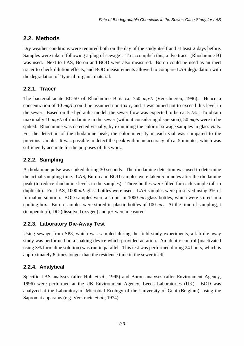
Fate of Biodegradable Chemicals in the Sewer: Case Study for LAS
- 9.3 -
2.2. Methods
Dry weather conditions were required both on the day of the study itself and at least 2 days before.
Samples were taken ‘following a plug of sewage’. To accomplish this, a dye tracer (Rhodamine B)
was used. Next to LAS, Boron and BOD were also measured. Boron could be used as an inert
tracer to check dilution effects, and BOD measurements allowed to compare LAS degradation with
the degradation of ‘typical’ organic material.
2.2.1. Tracer
The bacterial acute EC-50 of Rhodamine B is ca. 750 mg/L (Verschueren, 1996). Hence a
concentration of 10 mg/L could be assumed non-toxic, and it was aimed not to exceed this level in
the sewer. Based on the hydraulic model, the sewer flow was expected to be ca. 5 L/s. To obtain
maximally 10 mg/L of rhodamine in the sewer (without considering dispersion), 50 mg/s were to be
spiked. Rhodamine was detected visually, by examining the color of sewage samples in glass vials.
For the detection of the rhodamine peak, the color intensity in each vial was compared to the
previous sample. It was possible to detect the peak within an accuracy of ca. 5 minutes, which was
sufficiently accurate for the purposes of this work.
2.2.2. Sampling
A rhodamine pulse was spiked during 30 seconds. The rhodamine detection was used to determine
the actual sampling time. LAS, Boron and BOD samples were taken 5 minutes after the rhodamine
peak (to reduce rhodamine levels in the samples). Three bottles were filled for each sample (all in
duplicate). For LAS, 1000 mL glass bottles were used. LAS samples were preserved using 3% of
formaline solution. BOD samples were also put in 1000 mL glass bottles, which were stored in a
cooling box. Boron samples were stored in plastic bottles of 100 mL. At the time of sampling, t
(temperature), DO (dissolved oxygen) and pH were measured.
2.2.3. Laboratory Die-Away Test
Using sewage from SP3, which was sampled during the field study experiments, a lab die-away
study was performed on a shaking device which provided aeration. An abiotic control (inactivated
using 3% formaline solution) was run in parallel. This test was performed during 24 hours, which is
approximately 8 times longer than the residence time in the sewer itself.
2.2.4. Analytical
Specific LAS analyses (after Holt et al., 1995) and Boron analyses (after Environment Agency,
1996) were performed at the UK Environment Agency, Leeds Laboratories (UK). BOD was
analyzed at the Laboratory of Microbial Ecology of the University of Gent (Belgium), using the
Sapromat apparatus (e.g. Verstraete et al., 1974).
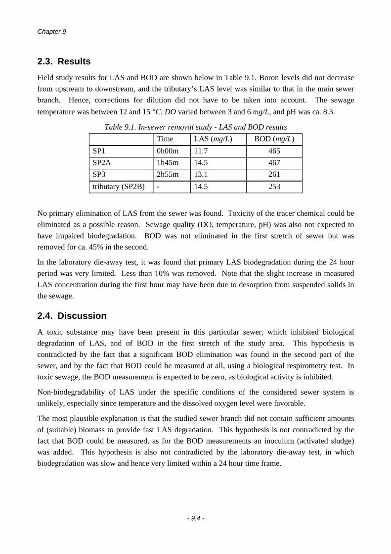
Chapter 9
- 9.4 -
2.3. Results
Field study results for LAS and BOD are shown below in Table 9.1. Boron levels did not decrease
from upstream to downstream, and the tributary’s LAS level was similar to that in the main sewer
branch. Hence, corrections for dilution did not have to be taken into account. The sewage
temperature was between 12 and 15 °C, DO varied between 3 and 6 mg/L, and pH was ca. 8.3.
Table 9.1. In-sewer removal study - LAS and BOD results
Time LAS (mg/L) BOD (mg/L)
SP1 0h00m 11.7 465
SP2A 1h45m 14.5 467
SP3 2h55m 13.1 261
tributary (SP2B) - 14.5 253
No primary elimination of LAS from the sewer was found. Toxicity of the tracer chemical could be
eliminated as a possible reason. Sewage quality (DO, temperature, pH) was also not expected to
have impaired biodegradation. BOD was not eliminated in the first stretch of sewer but was
removed for ca. 45% in the second.
In the laboratory die-away test, it was found that primary LAS biodegradation during the 24 hour
period was very limited. Less than 10% was removed. Note that the slight increase in measured
LAS concentration during the first hour may have been due to desorption from suspended solids in
the sewage.
2.4. Discussion
A toxic substance may have been present in this particular sewer, which inhibited biological
degradation of LAS, and of BOD in the first stretch of the study area. This hypothesis is
contradicted by the fact that a significant BOD elimination was found in the second part of the
sewer, and by the fact that BOD could be measured at all, using a biological respirometry test. In
toxic sewage, the BOD measurement is expected to be zero, as biological activity is inhibited.
Non-biodegradability of LAS under the specific conditions of the considered sewer system is
unlikely, especially since temperature and the dissolved oxygen level were favorable.
The most plausible explanation is that the studied sewer branch did not contain sufficient amounts
of (suitable) biomass to provide fast LAS degradation. This hypothesis is not contradicted by the
fact that BOD could be measured, as for the BOD measurements an inoculum (activated sludge)
was added. This hypothesis is also not contradicted by the laboratory die-away test, in which
biodegradation was slow and hence very limited within a 24 hour time frame.

Fate of Biodegradable Chemicals in the Sewer: Case Study for LAS
- 9.5 -
3. Laboratory Experiments
As the results of the field study did not meet the expectations based on literature, a further
laboratory experiment was conducted to measure the biological degradation kinetics of LAS in Tielt
sewage under different biomass conditions. To examine the effect of the specific sewage origin, a
die-away experiment was also conducted with Gent sewage (WWTP influent).
3.1. Methods
3.1.1. Sampling
Tielt sewage: a composite sewage sample was taken at Tielt SP2A. In total, 10 L of sewage was
collected and transported to the lab, stored in a cooling box. Next to the sewage sample, a sewer
sediment sample (200 mL)was taken. Gent sewage: influent of the Gent WWTP (Ossemeersen) was
sampled. 2 L of sewage was taken and transported to the lab, stored in a cooling box. Activated
sludge, required for a die-away study with inoculum, was also taken from this WWTP in Gent (100
mL of recycle sludge).
3.1.2. Experiments
The die-away study was performed during 5 days. Different types and levels of bacterial inoculum
were used for the different experiments (Table 9.2).
Table 9.2. Description of sewage die-away experiments
Name Sewage Description
A, B Tielt SP2A sewage, as such 2x
C, D Tielt SP2A + Tielt sewer sediment (5% v/v) 2x
E, F Tielt SP2A + Ossemeersen activated sludge (5% v/v) 2x
G Tielt SP2A abiotic control (3% v/v formaline solution) 1x
H Gent influent, as such 1x
The sewage samples were put in open glass bottles, at room temperature, and were mixed (and
aerated) on a shaking platform during 5 days. The sampling intensity was decreased towards the
end of the experiments, as an exponential decay profile was expected. Samples for surfactant
analysis (50 mL) were preserved with 3% formaline solution. pH, DO and temperature were
regularly monitored and adjusted if needed. A DO level between 3 and 4 mg/L was aimed for, as
this is representative of the situation in the considered sewer system.
At the start of the experiment, the water temperature was less than 20 °C, as the samples were
previously stored in a refrigerator. During the first day temperature increased to > 27 °C, due to
very high ambient temperatures. The next days temperature stabilized between 23 and 25 °C.
Chapter 9
- 9.6 -
3.1.3. Analytical
To reduce the costs of the experiment, an aspecific analytical method for anionic surfactants was
used: the Azure-A method (Den Tonkelaar & Bergshoeff, 1969). The measurements were
performed at Procter & Gamble Euro-Analytical (Strombeek-Bever, Belgium). The BOD of Tielt
SP2A was measured, using the Sapromat apparatus, without the addition of an inoculum (but with
the normal addition of a nitrification inhibitor) (Laboratory of Microbial Ecology of the University
of Gent, Belgium).
3.2. Results
The Tielt SP2A raw sewage, as such, was used for a non-inoculated BOD measurement. The 10
day BOD value (at 20 °C) was 565 mgO2/L (average of duplicate analyses). From the BOD curves,
it could be derived that sufficient numbers of competent micro-organisms were present in the raw
sewage for the fast degradation of organics, without the need for an adaptation phase.
The results (expressed as % remaining Azure-A active substances) are plotted in Figure 9.2 (the
mean value is given for duplicate experiments).
0 20 40 60 80 100 120Time (h)
Ani
onic
sur
fact
ants
(%
of o
rigin
al v
alue
)
Tielt abioticGent
0%
20%
40%
60%
80%
100%
120%
0 20 40 60 80 100 120
Time (h)
Tielt as suchTielt + sedTielt + AS
0%
20%
40%
60%
80%
100%
120%
Figure 9.2. Sewage die-away experiments: % remaining anionic surfactants
Approximately 30% of the anionic surfactants was removed in the abiotic control. Anionic
surfactants degradation in Tielt sewage was faster than in Gent sewage. The fitted first-order decay
rate in Tielt (average for all 3 experiments) was 0.021 h-1, while the fitted rate for the Gent
experiment was only 0.013 h-1. There was no influence of adding extra biomass (from sewer
sediment or from activated sludge) on the rate of anionic surfactants degradation in Tielt sewage.
3.3. Discussion
It was found that Tielt sewage contained sufficient competent biomass for the degradation of BOD,
as shown by the Sapromat experiment without inoculum. Tielt sewage showed no toxicity towards
BOD degrading micro-organisms.

Fate of Biodegradable Chemicals in the Sewer: Case Study for LAS
- 9.7 -
Elimination of anionic surfactants was faster in Tielt sewage than in Gent sewage. The primary
surfactant removal was complete in both cases, but it required 50 hours for Tielt and 80 hours for
Gent. From these kinetics, the field study results can be explained. The half-life time for the decay
of anionic surfactants in Tielt sewage was 34.5 h. This is a factor 10 higher than the actual
residence time in the studied sewer line, which explains the absence of any measurable LAS
elimination.
There was no difference in anionic surfactants elimination between the sewage ‘as such’
experiments and the experiments with additional biomass. Apparently, the addition of only 5%
(v/v) of an extra biomass source (sewer sediment or activated sludge) was not sufficient to speed up
biodegradation.
4. Modeling Exercise
The method used by Matthijs et al. (1995, 1997) and Holt et al. (1998), based on market data and
measured WWTP influent concentrations, was applied to the Tielt study area. Market data for
anionic surfactants in the region of Tielt were provided by Procter & Gamble, Eurocor. Inhabitant
numbers and water consumption were obtained from Aquafin. These data, together with the
predicted concentration of anionic surfactants in the 2 sewer branches at the location SP2A, is given
in Table 9.3.
Table 9.3. Prediction of anionic surfactants concentration in Tielt SP2A sewage
Sewer branch Inhabitants
(cap)
Water use
(L.cap-1.day-1)
Anionics use
(g. cap-1.day-1)
Anionics conc.
(predicted - mg/L)
Aarsele center 1097 87 5.1 59
Baudeloostraat 269 136 38
The weighted average (by flow) of the anionics concentration in the 2 considered branches is 53
mg/L. The measured concentration was 17.5 mg/L. Based on this, a removal efficiency of 67% can
be derived. This compares well with the removals mentioned in the literature.
It should be noted that the measured concentration only represents one point of the diurnal
concentration curve. As the sample was taken around 11h00 AM, it is expected to represent a high
but not the maximal value.

Chapter 9
- 9.8 -
5. Discussion
The results of the field study presented in this chapter appear to be in contradiction with the in-
sewer removal measurements described in the literature. On the other hand, based on a comparison
of the predicted raw sewage concentration and the measured concentration, the anionic surfactants
appeared to have been removed to a large extent upstream in the sewer system.
The field study described in this chapter indicated that in the main sewer line of Aarsele (Tielt), no
LAS removal occurred. The laboratory sewage die-away studies showed a complete elimination of
anionic surfactants, but at a relatively slow rate. This confirmed that, based on the activity of
suspended biomass in the considered sewage, biodegradation was too slow to achieve any
significant removal in the 3 hours residence time. On the other hand, the absence of in-sewer
removal is contradicted by the modeling exercise.
None of the studies mentioned in the literature were conducted by means of a dye-tracer experiment.
None of them gives a full confirmation about the processes which occurred in a specific ‘packet’ of
sewage. The field study presented here showed no LAS removal following such a packet of sewage
in a single stretch of the main sewer. However, the high LAS removal degrees found in the studies
given in the literature were related to the entire sewer system, instead of one stretch. Considering
the entire sewer system in Aarsele (using the market data modeling approach), a high degree of
removal was also found.
A possible explanation is that no surfactant in-sewer removal took place in the main sewer line
because no biofilm could be established there due to intermittent flushing by the upstream pump.
On the other hand, biofilms are expected to be present and active in the slower flowing side
branches of the system. Assuming the results of the market data approach are correct, a high degree
of surfactant elimination must have taken place in these smaller side branches.
To gain a better understanding of the fate of chemicals in the sewer system, it is recommended that
a detailed monitoring campaign be conducted. The chemical fate pathway should be followed from
the households to the treatment plant or to the main sewer line. An entire sewer (sub)catchment
should be evaluated, preferably under completely controlled conditions, and using tracer chemicals.
Therefore, co-operation of the area’s inhabitants is most probably required (cf. the experiments by
Schowanek et al., 1996).

Chapter 10 -
New PEC Definitions for River Basins Applicableto GIS-based Environmental Exposure
Assessment
this chapter was submitted for publication as:
Boeije, G., Wagner, J.-O., Koormann, F., Vanrolleghem, P., Schowanek, D. & Feijtel, T.C.J.
(submitted). New PEC definitions for river basins applicable to GIS-based environmental exposureassessment. Submitted to Chemosphere.

- 10.1 -
Chapter 10
New PEC Definitions for River Basins Applicableto GIS-based Environmental ExposureAssessment
1. Introduction
The initial output of a GREAT-ER simulation (Feijtel et al., 1997; Boeije et al., 1997) for a specific
catchment and chemical is a set of geo-referenced local predicted concentrations, linked to a digital
river network. This can e.g. be presented as a color-coded map or as a concentration profile. Such
output is directly applicable for local (or regional) water quality management purposes, and it allows
model verification by means of site-specific monitoring programs. Moreover, it allows the
identification of local high risk areas. However, for application in a regional environmental risk
assessment context, there is a need to aggregate the geo-referenced output to a single value (or
frequency distribution) which is representative of chemical exposure within the catchment.
In this chapter, two aggregation methods were studied: aggregation of all concentrations in the
catchment, and aggregation of all ‘highest’ predicted concentrations (occurring immediately below
waste water emission points).
2. Definitions
2.1. Nomenclature
Local (frequency distributions of) concentrations are linked to individual river stretches or waste
water emission points. As the acronym ‘PEC’ is a regulatory term (e.g. EEC, 1994b), which is used
in risk assessment for comparison with PNECs or NOECs, this is not to be used for predicted local
geo-referenced concentrations. Instead, the term ‘CSIM’ (simulated concentration) was applied.
For each stretch, GREAT-ER simulations produce the values CSIM,start (at the beginning of the
stretch), CSIM,end (at the end of the stretch) and CSIM,internal (predicted average concentration in the
stretch) (chapters 2 and 3 of this thesis).
In this chapter, aggregated concentration values - which can be used in a risk assessment context -
are called PECs (Predicted Environmental Concentrations). Two aggregated PEC types were
defined and tested: PECinitial and PECcatchment.

Chapter 10
- 10.2 -
2.2. PECinitial
PECinitial is the spatial aggregation of concentrations in the river immediately after emissions. This
is comparable to PEClocal as defined in the EU Technical Guidance Documents (EEC, 1994b),
although its calculation method is different.
2.2.1. Local Basis for Spatial Aggregation
CSIM,start was selected as the starting point from which PECinitial can be calculated. This value can be
monitored (albeit indirectly), by calculating the mass balance of upstream and waste water effluent
measurements (both flow rate and concentrations), assuming complete instantaneous mixing. As no
in-stream removal below the emission point is considered, CSIM,start is independent of the river
segmentation (length of the stretches) and hence of the river network’s scale. CSIM,start is totally
scale independent if emissions are not aggregated into larger hypothetical emission points.
However, if aggregated emissions are used (i.e., if several small emission points are aggregated into
one hypothetical emission point), the CSIM,start value may increase.
The impact of the uncertainty around in-stream removal and flow velocity is limited to its impact on
the upstream concentration - it has no effect on the concentration which is due to the considered
waste water emissions. It can be concluded that CSIM,start offers the most stable and unambiguous
starting point for a PECinitial aggregation.
The fact that in-stream removal is not taken into account for the considered emission points results
in the use of the highest CSIM values produced by GREAT-ER simulations. This is complementary
to the PECcatchment approach (see below), where average values are used. It is stressed that CSIM,start
of an emission-receiving river only represents the ‘worst-case’ predicted in the one-dimensional
GREAT-ER river modeling approach. In reality, much higher concentrations can be found close to
the emission point, due to incomplete mixing. The true worst-case situation in the river occurs at
the exact location where the effluent is discharged into the river. At this point, no mixing or
dilution have yet occurred, and hence the local concentration in the river is equal to the effluent
concentration.
2.2.2. Spatial Aggregation
PECinitial is described by the spatial mean and spatial standard deviation of the local CSIM,start values.
The aggregation can be based on local means, or on local high percentiles (e.g. 90th) if a variability
analysis was included in the simulation. Weighting is not required in the spatial aggregation
process, as the unweighted approach is already scale-independent (CSIM,start is scale-independent in
itself). The unweighted approach warrants that all emission points are given equal importance.

New PEC Definitions for River Basins Applicable to GIS-based Environmental Exposure Assessment
- 10.3 -
2.3. PECcatchment
PECcatchment is the spatial aggregation of concentrations representative of the entire catchment.
Although this is a new concept typical for geo-referenced exposure assessment, but it could be
compared to PECregional in the EU Technical Guidance Documents (EEC, 1994b).
2.3.1. Local Basis for Spatial Aggregation
CSIM,internal is the most representative value for the concentration in a stretch. As PECcatchment aims to
provide a measure for the ‘representative’ concentration all over a catchment, it was based on this
most representative value for individual stretches. The CSIM,internal value of individual stretches is
scale dependent, as its calculation depends on the stretch length. The longer a stretch is, the more
residence time is available for in-stream removal, hence the average concentration CSIM,internal will
be lower in long stretches compared to short stretches (when all other conditions are equal). This
scale-dependency needs to be compensated for in the aggregation process.
2.3.2. Spatial Aggregation
PECcatchment can be described by the spatial mean and spatial standard deviation of the local
CSIM,internal (mean or high percentile) values.
Stretch selection
There are 2 plausible options for the selection of stretches which are to be included in the spatial
aggregation: (1) selection of all stretches in the digital river network (entire digitized catchment), or
(2) selection of only those stretches which are downstream of pollution sources.
Option (1) is the most comparable with the current regional exposure assessment approach (‘unit
world’ models, e.g. Mackay et al., 1992), in which all surface waters in a region are considered for
the dilution of the chemical mass loading. It allows to compare the degree of chemical-specific
pollution between catchments, and it also allows a quantitative evaluation of chemical-related water
quality in a catchment, which is especially useful from a water quality management point of view.
Option (2) focuses on polluted surface waters only. This is significantly different from the currently
used methods. However, this concept may also be appropriate for risk assessment: risk assessment
of the aquatic environment should mainly focus on rivers that are actually at risk (because they are
downstream of pollution points) and need not necessarily deal with pristine environments. A
practical reason in favor of this option is the fact that data on upstream unpolluted rivers
(headwaters) are generally scarce and/or of low quality, especially when large-scale databases and
maps are used.

Chapter 10
- 10.4 -
Scale-dependency
An unweighted spatial aggregation of predicted river concentrations can be identified as scale-
dependent in two ways: (A) related to the level of geographical detail of the river network, and (B)
related to the applied river stretch length:
(A) River network geographical detail
The unweighted aggregated PECcatchment is influenced by the number of upstream unpolluted rivers
which are included in the digital river network. The more unpolluted headwaters are present, the
lower the aggregated PECcatchment will be. The number of headwaters in the river network depends
not only on the digitization but also on the type of catchment: mountainous catchments will
typically have more (but smaller) sources than lowland catchments. This scale-dependency is
illustrated by means of the example river network in Figure 10.1. If all headwater stretches are
included (situation I), the unweighted average PECcatchment is 0.15. If on the other hand only the
three most downstream stretches are considered in the network (situation II), the unweighted
average PECcatchment is 0.50. This scale-dependency is resolved when headwater stretches are not
considered (situation III): in this case the unweighted average PECcatchment is 0.75, independent of
the upstream river network’s level of detail.
0
00
0
0 1
values = predicted concentrations
0
0.5
00
0 1 0.5
1 0.5
1 0.59 0.41
I
II
III
IV
= emission point
Figure 10.1. Scale-dependency of PECcatchment calculations: example river network

New PEC Definitions for River Basins Applicable to GIS-based Environmental Exposure Assessment
- 10.5 -
(B) Stretch length
In practice, river stretch length can not be fixed, e.g. due to the presence of confluences. Because of
this, the unweighted aggregated PECcatchment is influenced by the river segmentation. If in the
example river network of Figure 10.1 the most downstream stretch (with concentration 0.5) would
be split up into 2 stretches (situation IV), the unweighted average PECcatchment (based on the
selection of only those stretches downstream of pollution sources) would be 0.67 instead of 0.75.
Weighting
Because of both scale-dependencies, an unweighted spatial aggregation of CSIM,internal values can not
be used for PECcatchment calculations. PECcatchment would not be comparable between catchments
that were digitized at a different scale or using different stretch lengths, and would not be a constant
within a single catchment if it would be modeled using different scales or river segmentations.
Moreover, it would be possible to steer the value of PECcatchment by modifying the number of
considered headwaters, or by modifying the river segmentation.
Weighted by stretch length
Weighting by stretch length obviously solves scale-dependency (B) mentioned above. However, it
does not solve scale-dependency (A), related to the number of unpolluted headwaters that are
considered in the aggregation. Hence, this approach can only be applied in combination with option
(2) for stretch selection: only the stretches downstream of pollution sources.
The ecological interpretation is that equal importance is attached to rivers with equal length. Hence,
small rivers are considered equally valuable as large rivers. This attaches importance to the entire
aquatic ecosystem (the bulk water as well as the river’s edges), and also the terrestrial environment
near the river which is influenced by it.
The weights wi for each stretch i can be calculated as:
wl
li
i
jj
nstretches=
=∑
1
[10.1]
Weighted by flow increment
Weighting by flow increment in a stretch solves both scale dependencies (A) and (B). For the PEC
analysis, the flow increment in a stretch (i.e., the increase of flow in a stretch) is defined as the
difference in mean flow between the considered stretch and the upstream stretch. After a
confluence, the sum of both upstream flows is used. For the most upstream stretches in the digital
river network (i.e., which are not connected to any further upstream stretches), the flow increment is
equal to the flow itself. Hence, the flow increment in these most upstream stretches is equal to the
flow increment in the entire headwaters subcatchment which - in reality - feeds into them.

Chapter 10
- 10.6 -
This concept is illustrated in Figure 10.2 below. The flow increment ∆Q3 in stretch 3 is calculated
as the difference of the flow in stretch 3 with the upstream flow (i.e. the sum of flows in stretches 1
and 2). For stretches 1 and 2, there are no upstream stretches: the ‘upstream’ flows are zero, and
consequently the flow increment values ∆Q1 and ∆Q2 are equal to the flows in stretches 1 and 2.
For stretch 1, which in reality does receive the outflow of an upstream headwaters subcatchment, it
is shown in Figure 10.2 that the flow increment ∆Q1 corresponds with the entire headwaters
catchment, rather than with the drainage area of only stretch 1 itself.
1 2
31 2
3
Reality Digital River Network
∆Q1 = Q1 - 0 = Q1∆Q2 = Q2 - (Q1+Q3)∆Q3 = Q3 - 0 = Q3
Figure 10.2. Flow increment: schematic illustration of the concept
Weighting by flow increment assigns the weight of all headwaters which are in reality at more
upstream locations to the ‘most upstream’ stretches in the digital river network. This way, scale-
dependency (A) is resolved: digitizing more or less unpolluted headwaters has no influence on the
flow (= flow increment) in the most upstream stretch that is considered. However, it is crucial that
these most upstream stretches be free of pollution. If not, the concentration of a single polluted
stretch is given the weight of the entire (unpolluted) headwaters subcatchment feeding into this
stretch, and hence the PECcatchment is a gross overestimation of the true situation.
As flow increment is correlated with the drainage area of a stretch and hence also with stretch
length, scale-dependency (B) is also resolved. If a stretch is split into 2 sub-stretches, the sum of the
flow increment in both stretches is equal to the flow increment in the original stretch.
The ecological interpretation of this weighting approach is similar to the ‘weighted by stretch
length’ approach. However, stretches receiving emissions may have a higher weight, because the
waste water emission adds to the flow increment in a stretch.

New PEC Definitions for River Basins Applicable to GIS-based Environmental Exposure Assessment
- 10.7 -
The weights wi for each stretch i can be calculated as follows in equation [10.2]. Note that the total
flow increment in a catchment (i.e. the sum of the flow increments in all stretches) must necessarily
be equal to the flow at the end of the catchment.
wQ
Q
QQi
i
jj
ni
endstretches
= ≡
=∑∆
∆
∆
1
[10.2]
Weighted by stretch volume
The volume of a river stretch can be calculated from its flow, flow velocity and length. Hence, this
approach implicitly contains a weighting by length, and hence it solves scale-dependency (B).
Although this weighting approach decreases the importance of individual headwater stretches (due
to the implicit weighting by flow) it does not solve scale-dependency (A): a large number of
headwater stretches will - together - still contribute significantly to the weighted average. Hence,
this approach can only be applied in combination with the selection of only the stretches
downstream of pollution sources.
Weighting by stretch volume focuses on large rivers (because these have the largest volume). This
may be of less ecological relevance, as smaller rivers are often more valuable or vulnerable than
large ones. Also, weighting by volume stresses the importance of ‘bulk water’ organisms rather
than the benthic or river edge ecosystem. From an exposure assessment point of view, weighting by
volume focuses on high dilution situations, where risk and exposure levels may be lower than what
is representative for the entire catchment.
The weights wi for each stretch i can be calculated as:
wV
V
Q lv
Q l
v
istretch i
stretch jj
n
i i
i
j j
jj
nstretches stretches
= =
⋅
⋅
= =
∑ ∑
1 1
[10.3]
Additional weighting factors
Additional weighting factors can be considered (to be used in combination with one of the already
mentioned approaches). Additional weighting by flow directs the focus towards the main
waterbodies of the catchment. As with the volume-weighting, this focuses on large rivers, on high
dilution and on ‘bulk water’ organisms. Additional weighting by a water quality index will stress
the importance of high-quality ecosystems in the catchment. This will typically increase the weight
of stretches with a low degree of pollution and will hence decrease the aggregated PECcatchment,
possibly resulting in a too optimistic exposure assessment. Another problem with water quality
weighting is that the required data may not be generally or readily available, or not related to the
correct river network structure. Moreover, for different catchments the water quality indices may
not be comparable.

Chapter 10
- 10.8 -
In this chapter, additional weighting factors will not be further considered.
Calculation of weighted average and standard deviation
A weighted average is calculated as follows ( xW = weighted average, xi = individual values, n =
number of values):
x x wW i ii
n
= ⋅=∑
1
with wii
n
=∑ =
1
1 [10.4]
The weighted variance σ2W is an estimator of the population’s true variance, just like the ‘normally
calculated’ variance σ2 is one. However, a different probability function f(x) is used, reflecting a
non-aselective sampling approach of the population. For the ‘traditional’ calculation of variances,
an aselective sampling is represented by assigning equal probability to each xi: f(xi)=1/n. For the
weighted calculation, the probability for each xi is equal to its weight: fW(xi)=wi.
( ) ( )
( ) ( )
σ
σ
2 2 2
2 2 2
1( ) ( ) ( ) ( )
( ) ( ) ( ) ( )
x x E x f x dx x E xn
dx
x x E x f x dx x E x w dxW W i
= − ⋅ ⋅ = − ⋅ ⋅
= − ⋅ ⋅ = − ⋅ ⋅
−∞
+∞
−∞
+∞
−∞
+∞
−∞
+∞
∫ ∫
∫ ∫[10.5]
In the above integrals, the factors 1/n and wi are not relevant as they approach zero. However, when
the number of sampled values is finite, these integrals can be calculated as the corresponding sums.
Because these estimators for the variance are only unbiased asymptotically with n going to infinity,
a correction is required: the terms of the sums are to be multiplied by n/(n-1):
( )( )( )
σ 2 2
1
2
11
1 1( )x x x
nn
n
x x
ni
ni
n
= − ⋅ ⋅−
=−
−=
=∑∑
[10.6]
For the weighted calculation of the variance, the same correction was applied. Hence, when all
weights are equal to 1/n (i.e., the unweighted case), the weighted variance is equal to the variance
obtained in the ‘traditional’ calculation:
( ) ( )( )σW W ii
n
W ii
n
x x x wn
nx x w
nn
2 2
1
2
11 1( ) = − ⋅ ⋅
−
= − ⋅ ⋅−= =
∑ ∑ [10.7]

New PEC Definitions for River Basins Applicable to GIS-based Environmental Exposure Assessment
- 10.9 -
3. Case Studies
3.1. Methods
The applied fate model used a chemical specific percentage elimination to describe removal in the
sewer system and in waste water treatment (trickling filter or activated sludge). To calculate fate in
rivers, a fixed first-order in-stream removal rate coefficient was used. A Monte Carlo simulation
(1000 shots) was applied for simultaneous uncertainty and variability analysis. When uncertainty
and variability are combined, this method only offers reliable calculations of the local CSIM
distribution means, because the uncertainty increases the spread of the distributions (see chapter 2 of
this thesis). Consequently, only the mean CSIM values could be used for spatial aggregation in these
case studies.
A non-calibrated fate simulation was conducted for the surfactant LAS (Linear Alkylbenzene
Sulphonate). Next to this, a simulation was also conducted for the hypothetical substance CONS: a
completely conservative chemical with the same emission profile as LAS. The chemical properties
and market data used for LAS were based on chemical industry data (ECETOC, personal
communication). Together with the parameters for CONS, the LAS parameters are given in Table
10.1.
Table 10.1. Chemical parameters used in the case study simulations
LAS CONS
Product consumption 1 kg/(cap.year) 1 kg/(cap.year)
In-stream removal rate 0.006 - 1.71 h-1 * 0 h-1
Removal in primary treatment 45 % 0 %
Removal in activated sludge treatment 98 % 0 %
Removal in trickling filter treatment 85 % 0 %
Removal in the sewer 25 % 0 %
* uniform distribution
The PEC calculations were applied to two Yorkshire catchments, the Went and the Calder. The
datasets were not yet completely quality-controlled, and may hence have contained errors.
Therefore, the analysis presented here should not be interpreted as a reliable exposure assessment,
but merely as a test of the proposed PEC definitions and calculation methodologies.
For the PECcatchment calculations, three different stretch selection options were used: 1A all stretches;
1B a reduced catchment containing all polluted stretches plus one stretch for each unpolluted
subcatchment; and (2) a reduced catchment containing only polluted stretches (Figure 10.3). 1A and
1B are two cases representing the same concept (‘all stretches’), but applied at a different level of
geographical detail. A description of both catchments and the effect of the applied stretch selection
is given in Table 10.2 below.
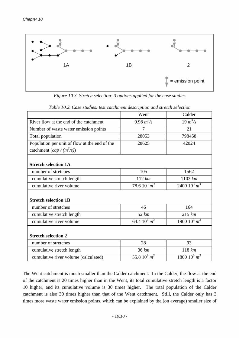
Chapter 10
- 10.10 -
1A 1B 2
= emission point
Figure 10.3. Stretch selection: 3 options applied for the case studies
Table 10.2. Case studies: test catchment description and stretch selection
Went Calder
River flow at the end of the catchment 0.98 m3/s 19 m3/s
Number of waste water emission points 7 21
Total population 28053 798458
Population per unit of flow at the end of the
catchment (cap / (m3/s))28625 42024
Stretch selection 1A
number of stretches 105 1562
cumulative stretch length 112 km 1103 km
cumulative river volume 78.6 103 m3 2400 103 m3
Stretch selection 1B
number of stretches 46 164
cumulative stretch length 52 km 215 km
cumulative river volume 64.4 103 m3 1900 103 m3
Stretch selection 2
number of stretches 28 93
cumulative stretch length 36 km 118 km
cumulative river volume (calculated) 55.8 103 m3 1800 103 m3
The Went catchment is much smaller than the Calder catchment. In the Calder, the flow at the end
of the catchment is 20 times higher than in the Went, its total cumulative stretch length is a factor
10 higher, and its cumulative volume is 30 times higher. The total population of the Calder
catchment is also 30 times higher than that of the Went catchment. Still, the Calder only has 3
times more waste water emission points, which can be explained by the (on average) smaller size of

New PEC Definitions for River Basins Applicable to GIS-based Environmental Exposure Assessment
- 10.11 -
the emissions into the Went. The total population divided by the river flow at the end of the
catchment is 1.5 times higher in the Calder than in the Went. Hence, the total domestic pollution
load in the Calder receives (in total) 1.5 times less dilution than that in the Went.
The number of stretches in selection 1A (all stretches of the 1:50,000 river network) was strongly
reduced when instead only the polluted stretches plus one unpolluted stretch per headwater
subcatchment, or strictly only the polluted stretches were used (stretch selection 1B;2). In the Went,
56;73 % of the stretches and cumulative stretch length disappeared. However, only 18;29 % of the
cumulative volume was lost. In the Calder, 90;94 % of the stretches and 80;89 % of the cumulative
length were removed, but again only 20;25 % of the cumulative volume. In the Calder catchment,
pollution is concentrated in the most downstream 6 % of the stretches, while in the Went more than
25 % of the stretches is influenced by pollution. The unpolluted volume fraction is much smaller,
which can be explained by the smaller volume of headwater stretches compared to the more
downstream parts of the rivers.
3.2. Results
The geo-referenced simulation results are illustrated in Figure 10.4 (Went) and Figure 10.5 (Calder)
(concentrations quartiles color-coded by means of gray-scale) (geographical projection).
Figure 10.4. Went simulation: LAS (top) and CONS (bottom)

Chapter 10
- 10.12 -
Figure 10.5. Calder simulation: LAS (top) and CONS (bottom)
3.2.1. PECinitial
PECinitial was defined as the unweighted spatial aggregation of CSIM,start for all stretches in the
catchment which directly receive an emission of waste water. The results of the PECinitial calculation
are given below in Table 10.3.
Table 10.3. PECinitial calculations (in mg/L)
Went Calder
mean st. dev. mean st. dev.
LAS 0.65 1.44 0.089 0.178
CONS 8.3 17.3 2.2 3.6

New PEC Definitions for River Basins Applicable to GIS-based Environmental Exposure Assessment
- 10.13 -
3.2.2. PECcatchment
PECcatchment was defined as the spatial aggregation of CSIM,internal values over the entire catchment, or
over the polluted section of the catchment. For the first option, weighting by flow increment is
required, while for the second option weighting by length or by volume is needed.
For LAS, the spatial variability of CSIM,internal values is shown in Figure 10.6. These histograms
were weighted by flow increment (‘all stretches’ case) or by stretch length (‘only polluted stretches’
case) - similar to the PECcatchment calculations (weighted histograms were obtained by counting the
cumulative weight instead of the frequency in each class). The left part of Figure 10.6 shows the
importance of unpolluted headwaters in the ‘all stretches’ case (peak at concentration zero); the
spatial distribution does not have a specific “standard” shape. In the right half of Figure 10.6, a
lognormal-like shape can be recognized for the Calder but not for the Went.
Calder - LAS - all stretches
0
0.1
0.2
0.3
0.4
0.5
0.6
0.7
0.8
0.9
0
0.00
2
0.00
4
0.00
6
0.00
8
0.01
0.01
2
0.01
4
0.01
6
0.01
8
0.02
C SIM,internal (mg/L)
Wei
gh
t
0%
20%
40%
60%
80%
100%Calder - LAS - only polluted stretches
0
0.05
0.1
0.15
0.2
0.25
0.3
0
0.00
5
0.01
0.01
5
0.02
0.02
5
0.03
0.03
5
0.04
0.04
5
0.05
C SIM,internal (mg/L)
Wei
gh
t
0%
20%
40%
60%
80%
100%
Went - LAS - all stretches
0
0.1
0.2
0.3
0.4
0.5
0.6
0.7
0.8
0
0.00
1
0.00
2
0.00
3
0.00
4
0.00
5
0.00
6
0.00
7
0.00
8
0.00
9
0.01
C SIM,internal (mg/L)
Wei
gh
t
0%
20%
40%
60%
80%
100%Went - LAS - only polluted stretches
0
0.1
0.2
0.3
0.4
0.5
0.6
0.7
0
0.01
0.02
0.03
0.04
0.05
0.06
0.07
0.08
0.09 0.
1
C SIM,internal (mg/L)
Wei
gh
t
0%
20%
40%
60%
80%
100%
weighted by flow increment weighted by stretch length
Mor
e
Mor
eM
ore
Mor
e
Figure 10.6. Spatial variability of CSIM,internal values (for LAS) (weighted histograms)

Chapter 10
- 10.14 -
In the PECcatchment calculations presented here, four different weightings (unweighted, by length, by
flow increment and by volume) were used in combination with the three different stretch selections
(see higher, section 3.1). Only the weighting techniques described above in the PECcatchment
definitions (section 2.3.2) are considered relevant; the results obtained with the other techniques are
given to illustrate their scale-dependency and hence their irrelevance. PECcatchment values are listed
in Table 10.4. Results obtained with scale-dependent calculations are printed in italics.
3.3. Discussion
3.3.1. Scale Dependencies in PECcatchment Calculations
Effect of reduction in catchment detail (1A versus 1B)
The type-A scale-dependency (linked to the number of unpolluted upstream stretches that are
considered in the river network) of the unweighted, weighted-by-length and weighted-by-volume
calculation approaches can be observed by comparing PECcatchment for stretch selection 1A and 1B.
When the number of unpolluted headwater stretches in the digital river network was reduced (i.e.,
when the network’s level of detail was decreased), PECcatchment increased in all cases. The volume-
weighted PECcatchment was least affected because the total volume of the headwater stretches has a
relatively low weight compared to the entire catchment’s volume: the reduction of the headwater
stretches only caused a 25-30 % decrease in total volume.
PECcatchment weighted by flow increment was independent of the number of considered unpolluted
headwater stretches. The minor differences between stretch selection 1A and 1B for the Calder
were due to inconsistencies in the flow data, which caused a negative flow increment for some
stretches. This also led to the not strictly monotonous behavior of the weighted cumulative
frequency distribution curves for the Calder in Figure 10.6.
The results confirm the theoretical considerations about scale dependency in section 2.3.2. It can be
concluded that for a PECcatchment calculation which aims to consider the entire catchment (both the
polluted and the unpolluted parts), weighting of CSIM,internal by flow increment is required.
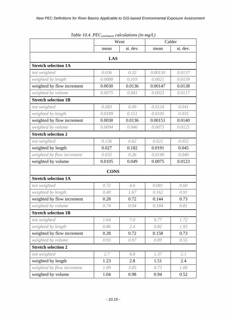
New PEC Definitions for River Basins Applicable to GIS-based Environmental Exposure Assessment
- 10.15 -
Table 10.4. PECcatchment calculations (in mg/L)
Went Calder
mean st. dev. mean st. dev.
LAS
Stretch selection 1A
not weighted 0.036 0.32 0.00130 0.0137
weighted by length 0.0088 0.103 0.0021 0.0159
weighted by flow increment 0.0030 0.0136 0.00147 0.0138
weighted by volume 0.0075 0.041 0.0023 0.0117
Stretch selection 1B
not weighted 0.083 0.49 0.0124 0.041
weighted by length 0.0189 0.151 0.0105 0.035
weighted by flow increment 0.0030 0.0136 0.00151 0.0140
weighted by volume 0.0094 0.046 0.0073 0.0121
Stretch selection 2
not weighted 0.136 0.62 0.022 0.052
weighted by length 0.027 0.182 0.0191 0.045
weighted by flow increment 0.032 0.26 0.0190 0.040
weighted by volume 0.0105 0.049 0.0075 0.0123
CONS
Stretch selection 1A
not weighted 0.72 4.6 0.081 0.60
weighted by length 0.40 1.67 0.162 0.91
weighted by flow increment 0.28 0.72 0.144 0.73
weighted by volume 0.74 0.94 0.184 0.81
Stretch selection 1B
not weighted 1.64 7.0 0.77 1.72
weighted by length 0.86 2.4 0.82 1.93
weighted by flow increment 0.28 0.72 0.158 0.73
weighted by volume 0.93 0.97 0.89 0.55
Stretch selection 2
not weighted 2.7 8.8 1.37 2.1
weighted by length 1.23 2.8 1.51 2.4
weighted by flow increment 1.09 3.85 0.73 1.00
weighted by volume 1.04 0.98 0.94 0.52

Chapter 10
- 10.16 -
Effect of stretch selection: all stretches (1A) versus only polluted stretches (2)
PECcatchment increased when only polluted stretches were used instead of the entire catchment. This
is straightforward, as average exposure levels are necessarily higher in the polluted sections of a
catchment compared to the zero-exposure in the unpolluted sections. In all cases, the PECcatchment
increase was higher in the Calder than in the Went. This can be explained by the catchments’
structure: as there are more unpolluted headwater stretches in the Calder compared to the Went,
dropping these headwaters from the calculations obviously has a stronger impact for a catchment
with more headwaters.
For the flow-increment weighted case, this was by more than a factor 10 for LAS and by a factor 4-5
for CONS. However, this calculation method is irrelevant in combination with stretch selection 2.
When only polluted stretches are considered, the weight of entire unpolluted headwater sub-
catchments is assigned to the situation of the most upstream polluted stretches into which these
headwaters feed (cf. Figure 10.2, assuming that stretch 1 would be polluted). Hence, such
calculations result in a strong overestimation of true exposure levels.
The spread of the spatial distributions decreased (in the Calder by a factor 3-8; in the Went by a
factor 1-2). This can be ascribed to the reduction in spatial variability when a large number of
‘extreme’ cases (zero concentration) are removed from the population. This can also be observed in
Figure 10.6.
For both catchments, the LAS PECcatchment based on only polluted stretches and weighted by volume
was a factor 2.5 lower than the corresponding PECcatchment weighted by length. This is in line with
the expectation that weighting by volume focuses the attention to larger rivers with higher dilution
and after more in-stream removal has taken place. For CONS a similar effect was seen (factor 1.6
for the Calder, factor 1.2 for the Went). The effect was less extensive because CONS is only
affected by dilution, not by in-stream removal. The spread of the volume-weighted PECcatchment was
also lower for both chemicals and catchments, which can be explained by the leveling out of very
high or low concentrations in the more downstream rivers.
Effect of river segmentation
The type-B scale-dependency (linked to the variable stretch length) of the unweighted PECcatchment
calculation (see section 2.3.2) could not be illustrated in this work, because the river network
segmentation itself was not modified.
3.3.2. Comparison of PEC Calculations and Catchments
PECinitial
For LAS, PECinitial was a factor 7 higher in the Went compared to the Calder. For CONS, the
difference between PECinitial in both catchments was smaller than for LAS (a factor 4). The higher
PECinitial of CONS in Went versus Calder can not be due to a different waste water treatment

New PEC Definitions for River Basins Applicable to GIS-based Environmental Exposure Assessment
- 10.17 -
infrastructure as the chemical is conservative. Also for LAS this is not probable, as in both
catchments the sewage is mainly treated by trickling filter plants. A plausible explanation is the
difference in catchment structure. On average, the emission points in the Went are at a more
upstream location than those in the Calder, hence they generally receive a lower dilution.
For LAS, the spread of the spatial PECinitial distribution was similar in both catchments (standard
deviation / mean ≅ 2). For CONS, the spread of the distribution in the Went was similar to the LAS
case, while for the Calder it was more narrow (st.dev. / mean ≅ 1.6).
The PECinitial for CONS was much higher than for LAS, which is obvious as CONS is not
eliminated in waste water treatment. Furthermore, as CONS undergoes no in-stream removal,
CSIM,start values associated with more downstream emission points also contain a major component
of upstream pollution, which further increases PECinitial.
PECinitial versus PECcatchment
As expected, PECinitial was always higher than PECcatchment. Compared to the weighted-by-flow-
increment PECcatchment considering all stretches, this difference was more than a factor 200;30
(LAS;CONS) for the Went and a factor 60;15 (LAS;CONS) for the Calder. The spread of PECinitial
was a factor 2-5 lower for LAS and a factor 1-3 for CONS. The lower spread is caused by the
relative similarity of concentrations immediately after emissions compared to the much larger
variability of concentrations all over the catchment.
When only the polluted stretches are considered, the difference with PECinitial is less spectacular.
For LAS;CONS in the Went, these PECcatchment values were lower by a factor 24;7 (weighted-by-
length) and 60;8 (weighted-by-length). In the Calder, the difference was limited to a factor 5;1.4
and 12;2.3. The difference between Went and Calder indicates that the pollution in the Calder is
more concentrated in the downstream sections of the catchment, resulting in a ‘polluted-only’
PECcatchment which is closer to PECinitial. In the Went, pollution is more spread out, hence relatively
more in-stream removal (for LAS) and extra dilution can take place, resulting in a ‘polluted-only’
PECcatchment which is farther away from PECinitial. The difference between LAS and CONS is due to
the absence of in-stream removal for the latter. For CONS, the difference between PECinitial and the
‘polluted-only’ PECcatchment is only due to additional dilution downstream of the emission points.
PECcatchment weighted by length, considering only polluted stretches
A neutral view on the situation in the polluted parts of a catchment (assuming equal importance for
all locations in the river) is represented by PECcatchment weighted by length, considering only
polluted stretches.

Chapter 10
- 10.18 -
LAS exposure levels calculated for the polluted part of the Went are a factor 1.4 higher than those in
the Calder. This can mainly be explained by the higher PECinitial in the Went. The fact that the ratio
between PECcatchment values of the Went and the Calder is much lower than the ratio between their
PECinitial values (factor 7), is mainly due to the different dilution properties in both catchments.
Contrary to LAS, the exposure to CONS in the polluted parts of the Went was slightly lower than in
the polluted parts of the Calder - even though PECinitial was higher in the Went by a factor 4. This
can only be ascribed to the different dilution in both catchments.
PECcatchment weighted by volume, considering only polluted stretches
When stretch volume is used for weighting instead of stretch length, the aggregated exposure level
dropped by a factor 2.5 for LAS and 1.2-1.6 for CONS. As mentioned higher, this is due to the fact
that weighting by volume attaches most attention to downstream stretches with high dilution and
after more in-stream removal. Note that in this weighting case, the exposure to CONS in the Calder
was slightly lower than in the Went (contrary to the weighted-by-length case presented above).
PECcatchment weighted by flow increment, considering all stretches
The overall exposure situation in a catchment can be measured by means of PECcatchment weighted
by flow increment, considering all stretches (polluted as well as unpolluted).
Both for LAS and CONS, PECcatchment weighted by flow increment in the Calder was a factor 2
lower than in the Went. This is due to two factors: it is directly determined by the lower PECinitial inthe Calder, and it is also influenced by the location of the emission points. As most emissions are
situated in the downstream regions, most of the Calder’s upstream sections are unpolluted, which
significantly reduces the average exposure over the entire catchment. This explains why the ratio
between the ‘all stretches’ PECcatchment values in the Went and the Calder is higher than the ratio
between the ‘polluted-only’ PECcatchment values. The difference in catchment structure also explains
why PECcatchment for CONS based on all stretches is lower in the Calder than in the Went, while
PECcatchment based on only the polluted stretches has a similar value in both catchments.

New PEC Definitions for River Basins Applicable to GIS-based Environmental Exposure Assessment
- 10.19 -
4. Conclusions
Two spatially aggregated PEC types were defined and tested: PECinitial and PECcatchment.
PECinitial was defined as the spatial aggregation of initial river concentrations after each waste water
emission in the catchment, by means of an unweighted average, based on mean or high percentile
concentrations.
PECcatchment was defined as the spatial aggregation of all ‘internal’ river concentrations (i.e., the
average value in a stretch), by means of a weighted average, based on mean or high percentile
concentrations. To obtain an aggregated exposure value representative of the entire catchment, all
stretches (polluted and unpolluted) have to be considered. In this case, weighting by flow increment
is needed to resolve scale-dependency. To produce an aggregated exposure value representative of
the polluted parts of the catchment, only the polluted stretches should be considered. In this case,
weighting by stretch length or by stretch volume is required to resolve scale-dependency.
Weighting by length results in a ‘neutral’ aggregation which attaches identical importance to all
locations in the river network. Weighting by volume stresses the importance of downstream parts
of the river with a higher dilution and after more in-stream removal, hence resulting in a lower
exposure estimate.
A higher PECcatchment in the polluted part of the catchment compared to the entire catchment is
obvious, and inherently part of the concept. It must be stressed that a PECcatchment based on only
polluted stretches is not representative of the entire catchment, and this should be taken into account
when such a PEC is applied in a risk assessment framework.
The irrelevance due to scale-dependency of an unweighted PECcatchment was illustrated. The need
for an adequate stretch selection as a function of the selected weighting technique was also shown.
It is stressed that the use of an inappropriate stretch selection / weighting combination results in an
aggregation which depends on the level of detail of the digital river network or on the geographical
scale. Such aggregations are irrelevant because they can not be compared between catchments or
between different digital versions of a single catchment. Consequently, as such values are not
unambiguously determined, they can not be compared with effects levels, and hence they can not be
used in environmental risk assessment.
Both proposed PECcatchment calculation methodologies do not require data about the entire river
network that is being studied. When only polluted stretches are considered, no data is needed about
the unpolluted sections of the catchment. When the entire catchment is considered, only the most
downstream unpolluted stretches are required to obtain a PECcatchment weighted by flow increment.
Hence, for the proposed PECcatchment calculations, fate simulations, flow data collection and river
network digitization are not required for the entire catchment, but only for a limited (downstream)
part. This may reduce the effort needed to implement the GREAT-ER methodology for new
regions, and it will strongly decrease the required simulation time.

Chapter 11 -
Conclusions and Perspectives

- 11.1 -
Chapter 11
Conclusions and Perspectives
1. Introduction
The work described in this thesis was conducted in the framework of the GREAT-ER project
(Geography-referenced Regional Exposure Assessment Tool for European Rivers). The objective
of this international project was to develop, test and corroborate an accurate exposure prediction
tool, to estimate chemical exposure concentrations in surface waters. Such tool could be used to
enhance the realism and accuracy of environmental risk assessment schemes used in the European
Union. Current techniques to calculate regional predicted environmental concentrations (PECs) use
a generic multimedia ‘unit world’ approach and do not account for spatial and temporal variability
in environmental characteristics and chemical emissions. Since these methods do not offer realistic
predictions of actual concentrations, the results are merely applicable on a generic screening level.
In the GREAT-ER project, a software system was developed to calculate predicted concentrations
of ‘down-the-drain’ chemicals (i.e., consumer chemicals which mainly enter the environment via
the domestic waste water route, e.g. detergents) in surface waters, using a Geographic Information
System (GIS) for data storage and visualization, combined with simple mathematical models for the
prediction of chemical fate.
The work described in this thesis was focused on chemical fate modeling and simulation, and on
interpretation of simulation results. First, the development and testing of the simulation
methodology was described. Next the selection, adaptation and/or development of appropriate
chemical fate prediction models, supported by new measurement methods, was discussed. Finally,
a method to obtain spatially aggregated PECs for catchment simulations was worked out.
2. Methodology
A geo-referenced simulation methodology for the prediction of aquatic exposure to individual
‘down-the-drain’ chemicals was developed. This method uses real-world data, including their
spatial and temporal variability. By means of a hybrid stochastic / deterministic simulation
approach, statistical frequency distributions of predicted concentrations in the aquatic environment
are obtained. Steady-state deterministic models, which describe chemical fate, form the system’s
core. From chemical market data, combined with information on the location of consumers and
their emission habits, geo-referenced domestic chemical emissions are predicted. These emissions

Chapter 11
- 11.2 -
are further processed in sewer and treatment models, to obtain predicted chemical mass fluxes into
rivers. These emission fluxes are entered into a river model, resulting in geo-referenced predictions
of chemical concentrations in the considered river systems. A stochastic (Monte Carlo) simulation,
which deals with the natural variability and/or the uncertainty in the required information, is applied
on top of these deterministic models. This finally results in statistical distributions of predicted
concentrations, which can be used for risk assessment.
A prototype of the presented simulation system was tested by means of a (hypothetical) large
sample data set, containing 16,000 geographical segments. A 1,000 shot Monte Carlo simulation
took less than 1.5 hours on a low-end Windows NT personal computer (Intel Pentium processor,
150 MHz). From a computing power point of view, this indicates the feasibility of the approach for
detailed regional or large-scale pan-European simulations.
The currently implemented stochastic simulation approach does not allow to split variability and
uncertainty analysis. To achieve this, a “two-dimensional” stochastic simulation will have to be
built into the concept. As this will quadratically increase the total number of iterations and hence
also the required computing time, such technique may necessitate to replace the Monte Carlo
simulation by more efficient sampling techniques, e.g. stratified sampling (“Latin hypercube”).
The practical applicability of the GREAT-ER simulation methodology was illustrated by means of a
hypothetical but realistic case study. The simulation approach allowed to analyze the impact of
different discharges and tributaries on the temporal and spatial distributions of predicted
concentrations in the hypothetical catchment. The resulting distributions were log-normal. For the
prediction of seasonality (i.e. the variability of river flows through the year), Monte Carlo
simulation was found to be superior to the alternative (discrete) ‘flow scenario’ approach. Also for
a complete uncertainty or variability analysis, Monte Carlo simulation is needed. However, to
quickly obtain initial results, the ‘flow scenario’ method may be useful. Finally, the scale-
independent character of the approach was explored, by upscaling from a detailed to a larger
geographical scale.
3. Measurement and Prediction of Chemical Fate
The three main steps in the fate pathway of ‘down-the-drain’ chemicals were dealt with: sewers,
waste water treatment, and rivers. For activated sludge waste water treatment, the SimpleTreatmodel was adapted to biological nutrient removal (BNR) plants. This adaptation was supported by
measurements in modified versions of the standard CAS test (Continuous Activated Sludge), also
incorporating BNR. For trickling filters, a new model was developed. The model was tested using
measurements obtained in a laboratory pilot-scale (200 L) trickling filter, and in full-scale plants.
To predict chemical fate in rivers, a novel modeling approach was worked out, including biofilm
activity. This development was supported by a lab-scale artificial river experiment and a field
study. Finally, a preliminary field study was conducted to analyze chemical fate in the sewer.

Conclusions and Perspectives
- 11.3 -
3.1. Chemical Fate in Waste Water Treatment Plants
3.1.1. Biological Nutrient Removal Activated Sludge WWTPs
There is a global increase of biological nutrient removal (BNR) ability in waste water treatment
practice. This caused the need to modify both the Continuous Activated Sludge (CAS) laboratory
test system and the mathematical fate model SimpleTreat, which are used to routinely assess the
elimination of substances in activated sludge waste water treatment plants.
Adaptation of the CAS Test
Two novel ‘single-sludge’ BNR bench-scale test systems were compared to the standard CAS unit:
the Behr and the CAS-UCT unit, with respectively 2 (anoxic / aerobic) and 3 (anaerobic / anoxic /
aerobic) biological reactors. Both units proved to be easy to handle and operate. A similar degree
of COD, N and P removal was achieved with the Behr and the CAS-UCT. The experimental results
compared well with IAWQ Activated Sludge Model No. 2 simulations and with similar full-scale
plants. A new synthetic sewage was designed for the modified CAS units: to be more representative
of real sewage than the standard OECD synthetic medium, to allow a good degree of BNR, and to
support stable unit operation. A batch respiration test indicated that the new medium is a reasonable
approximation of real domestic sewage. Although sludge settling was superior when real sewage
was used, it remained sufficiently stable with the synthetic sewage to permit a 3 month test duration.
The longer residence times applied in the BNR systems led to a reduction in effluent levels of
biodegradable chemicals (like the surfactant LAS) compared to the CAS test. A parent LAS
removal efficiency of 99.4% was found in both units, while the standard CAS was observed to have
98.6% removal. The role of the system’s different redox zones in the overall removal requires
further investigation for various types of chemicals.
The BNR units hold potential to be included in standard testing, complementary to the CAS system.
As nutrient removal performance was similar in both units, the less complex Behr system may be
preferable for standardization. As the CAS-UCT allows a higher flexibility, it has better
perspectives for research applications.
Adaptation of the SimpleTreat Model
Most chemical fate models which are used to predict the elimination of individual chemicals in
waste water treatment plants, have until now not incorporated biological nutrient removal aspects.
Two modified versions of the standardized model SimpleTreat were developed, to increase its
applicability to BNR plants. The modifications mainly focus on an improved description of sludge
recycling, and on the presence of different redox zones in the biological reactor (aerobic, anoxic,
anaerobic).
A more realistic description of sludge recycling, taking into account the water phase of these
recycles and the actual recycling ratios, was proposed. It was shown that this may have an impact

Chapter 11
- 11.4 -
on the fate prediction of highly volatile chemicals. To deal with BNR plant designs, two modeling
approaches were presented, both based on the UCT process template: a 6-box model derived
directly from SimpleTreat, and a more detailed 10-box model. Simulation results of both models
were compared to measured LAS removals in the three bench-scale CAS test units. The LAS
degradation rate coefficient was calibrated only using standard CAS test data, and was subsequently
used to predict the fate of LAS in two BNR plants. Both modified models were more accurate than
the standard SimpleTreat. The 10-box model was more accurate than the 6-box model, which
(slightly) underestimated removal. In general, this illustrated the improved predictive power of the
adapted models for the fate of readily biodegradable chemicals.
It is recommended to focus further research on the corroboration of these models for different
chemical types. Especially simulation and laboratory measurements of volatile and / or less easily
degradable substances would allow to further test the underlying assumptions. This should also
give more conclusive evidence on the relative performance of the 6-box versus the 10-box model.
3.1.2. Trickling Filter WWTPs
The development of a chemical fate model for trickling filters was presented, based on the
SIMPLEBOX / SimpleTreat approach combined with an existing biofilm diffusion / biodegradation
model. By means of a sensitivity analysis, it was shown that the properties of the chemical under
study determine which parameters are most important for the model. Flow, volume and suspended
solids data are needed for the specific plant that is modeled. For biodegradable substances, biofilm
thickness is a crucial parameter which is generally not measured - hence this value typically has to
be estimated from defaults. For volatile chemicals it is required to estimate the air flow through the
filter, which may also be difficult. Finally, the fraction of water in the filter’s pores is an important
parameter, which can be derived from hydraulic measurements.
To test the new model, LAS removal experiments were conducted in the laboratory using a 200 Lpilot-scale high-rate trickling filter unit. The design of this unit allowed a characterization of all
relevant model parameters (e.g. measurement of hydraulics and biofilm characteristics by
continuously recording the filter unit’s mass, biofilm analysis by examining carrier material taken
from the filter). Moreover it allowed an easy monitoring of the system’s performance. Using this
setup, steady-state removal of LAS was measured under different well-characterized operating
conditions, at high and normal LAS influent levels. The effect of the operating conditions (short
versus long recycle, high versus low recycle ratio) was insignificant. At normal LAS influent levels
(4 mg/L), LAS removal was in the order of 50 %, while a higher COD removal efficiency (70 - 90
%) was found. When a 3-4 times higher LAS level was present in the influent, the LAS elimination
increased to 90 %. This may be ascribed to biological adaptation, but it may also indicate a
different kinetic behavior at high concentrations. Further research (preferably using dynamic
experiments) is required to study the effect of biological adaptation to different LAS influent
concentrations on removal efficiency.

Conclusions and Perspectives
- 11.5 -
The new fate model was able to describe LAS removal in the pilot-scale filter using measured,
estimated or default (literature) parameter values. The same biodegradation rate constant Kb
(derived from activated sludge data) could be used in all experiments with a normal LAS influent
concentration. However, for the experiments with 3-4 times more LAS in the influent, a 3.5 times
higher Kb value was needed. This indicates a shortcoming of the fate model: it can only deal with
this situation by recalibration of the biodegradation rate coefficient.
The model was also successfully applied to predict the fate of LAS in two full-scale low rate
domestic trickling filter plants. A plant-specific calibration produced more accurate predictions
than the extrapolation of another plant’s calibration. However, if a relative deviation in the order of
10 % is deemed acceptable, such a plant-specific calibration appeared to be not strictly required.
In this work, only the biodegradation and sorption aspects of the model were confronted with
measurements, since only LAS was used as test chemical. To test the relevance and validity of
volatilization aspects, further research is needed. Furthermore, it is recommended to focus
additional detailed research on the effect of influent concentrations on LAS biodegradation rates,
and on the effect on these rates of adaptation to different concentrations.
After a further validation for different types of substances, the newly developed fate model may be
used to complement the activated sludge model SimpleTreat. The bottleneck to apply the model is
the characterization of hydraulic and biofilm related parameters: generally such information is not
available or even measurable, hence realistic default values need to be applied. In the worst case,
this may heavily increase the predictive uncertainty, and hence it may lead to questioning the
usefulness of the model as such.
The main design criterion for the presented pilot-scale trickling filter unit was that it should allow a
characterization of biofilm and hydraulic parameters. Because of its dimensions, high influent and
effluent flows, and maintenance requirements, its operation is too laborious and complex to allow
easy standardization. Moreover, it is not representative of low-rate domestic trickling filter plants.
From this, it can be concluded that this system has no potential for use in standard chemical fate
assessments.
3.2. Chemical Fate in Rivers
Based on a literature review, a conceptual steady-state river fate model was selected, considering the
processes degradation (hydrolysis, photolysis, biodegradation), sorption / sedimentation, and
volatilization. The existing river fate models have a number of shortcomings: photolysis is
described as a crude simplification; sorption / sedimentation can only be modeled as accurate as the
applied suspended solids sedimentation rate coefficient (which is often not known); and
biodegradation is typically considered in a non-physically-based way, requiring site-specific
calibration. In this thesis, a new in-stream biodegradation model, which considers both biofilm and
suspended biomass activity, was developed.

Chapter 11
- 11.6 -
To calibrate this model for the surfactant LAS, experimental data were obtained in a lab-scale
artificial river system, which allowed to collect accurate and reproducible in-stream biodegradation
data next to the required river characteristics. In these experiments, biodegradation was found to be
the only significant in-stream removal process of LAS. In this specific case (with a high biofilm
surface to water volume ratio) measurable biodegradation only occurred when biofilm was present.
Moreover, the biodegradation rate was proportional to the amount of biofilm in the system.
The parameters of the new in-stream biodegradation model, calibrated on the series of experimental
data obtained in the artificial river experiments, had realistic values. Using these calibrated
parameters as such, the model was subsequently corroborated by comparing its predictions to an in-
stream removal field study in the Red Beck, a small Yorkshire river. Only easy to collect or default
data were used as site-specific model parameters. The predicted overall LAS half-life (without any
calibration using the field data) was 2¾ h. This is less than 25 % slower than the in-stream removal
half-life measured in the field. Hence, the model’s accuracy was acceptable for use in the GREAT-
ER concept.
It is recommended that a further corroboration of the presented modeling approach be conducted,
especially based on other detailed field study data. The range of validity of the model and its
assumptions needs to be extended to other chemical substances and to other types of rivers. If such
further validation would be succesful, the newly developed modeling concept may be an important
step forward in predicting in-stream removal of biodegradable chemicals (or BOD in general) in
rivers.
3.3. Chemical Fate in Sewers
To confirm and to further quantify the elimination of LAS in sewers, an in-sewer removal
experiment was conducted. The concentration of LAS was measured at different points in a well-
characterized sewer branch, following the plug of sewage using a dye tracer. Next to this, a
laboratory sewage die-away experiment was performed. No in-sewer removal of LAS was found.
The laboratory studies confirmed that, based on the activity of suspended biomass in the considered
sewage, biodegradation was too slow to achieve any significant removal in the 3 hours residence
time in this sewer. These findings appear to be in contradiction with literature data. They were also
contradicted by a modeling exercise based on market data, which considered the entire sewer system
rather than only the main branch. To gain a better understanding of the fate of chemicals in the
sewer system, further detailed research is recommended.
4. Calculation of Predicted Environmental Concentrations
By means of GREAT-ER, accurate chemical fate simulations can be performed for the aquatic
environment. However, the resulting digital maps with predicted concentrations for individual river
stretches may contain too much local detail for practical risk assessment applications and decision
making. To increase the applicability of GREAT-ER in a regional risk assessment context, it is

Conclusions and Perspectives
- 11.7 -
desirable that the geo-referenced output be aggregated to a single value (or at most a frequency
distribution), which is representative of chemical exposure within a catchment.
Two spatially aggregated PEC types were developed. PECinitial is defined as the unweighted spatial
aggregation of river concentrations just downstream of waste water emissions. PECcatchment is
defined as the spatial aggregation of all average stretch concentrations. To be representative of the
entire catchment, all stretches have to be considered. In this case, weighting by flow increment (i.e.
the difference of outflow and inflow for each stretch) is needed to resolve scale-dependency. To
produce a value representative of the polluted parts of the catchment, only the polluted stretches
should be considered, and weighting by stretch length or volume is required. Weighting by length or
by flow increment results in a ‘neutral’ aggregation, which attaches identical importance to all
locations in the river network. Weighting by volume stresses the importance of downstream parts
of the river with a higher dilution and after more in-stream removal, hence resulting in a lower
exposure estimate. It is obvious that a higher PECcatchment will be obtained when considering only
the polluted part of the catchment compared to the entire catchment. This should be taken into
account when these PECs are applied in a risk assessment framework.
The new PEC definitions were tested using simulations for 2 case study catchments (Calder and
Went, Yorkshire, UK). This confirmed the theoretical considerations which led to the different
definitions, and illustrated the need for weighting to resolve scale-dependencies.
It was shown that both proposed PECcatchment calculation methodologies do not require data about
the entire river network that is being studied. As no or very limited information is needed about
unpolluted headwaters, relatively coarse digital river networks can be sufficient. This may reduce
the cost and effort needed to implement the GREAT-ER methodology for new regions, and it will
strongly decrease the required simulation time.
The new approaches to calculate PECs offer a scale-independent method to compare geo-referenced
exposure predictions of a chemical between different catchments. Because of the scale-
independence and the standardization of the calculations, they also allow the comparison of geo-
referenced exposure predictions with standardized effects data. Hence, the new PECs can be
applied in environmental risk assessments. However, additional research will be required to
delineate which effects data are most relevant for specific views on exposure in a catchment. For
example, organisms present in the sections of the catchment directly downstream of emissions (cf.
PECinitial) may be less sensitive or ecologically valuable than those in the unpolluted headwaters.
This issue also holds true for comparison between catchments: some catchments may deserve a
higher degree of protection than others.

Chapter 11
- 11.8 -
5. General Conclusions and Perspectives
The simulation methodology and chemical fate models presented in this thesis were incorporated in
the GREAT-ER system. They were linked with an ArcView based GIS / data base / user interface
and a hydrological model, which were developed by other partners in this project.
Outside the scope of this thesis, the system was (or is being) applied to several pilot study
catchments: e.g. in the UK (Yorkshire Ouse, 15,000 km2), in Italy (northern Lambro, 1,000 km2), in
Germany (Itter, 100 km2) and in Belgium (Rupel, 7,500 km2). An initial model calibration and
corroboration exercise for Boron and LAS indicated that GREAT-ER was able to predict
environmental exposure to these chemicals with an accuracy well within the originally required
factor 5. Generally, the predicted mean concentrations were within one standard deviation of the
monitored means. It can be concluded that GREAT-ER has the potential to complement the current
generic ‘unit world’ models (of which the realism and accuracy are much lower) in higher-tier
exposure assessments. Note that the calibration exercise also indicated that GREAT-ER
simulations can be used to track errors or inconsistencies in the geo-referenced environmental data
sets.
The main bottleneck to apply GREAT-ER is the difficulty and cost of geographical data collection,
due to the generally inhomogeneous formats in which environmental data are stored by different
authorities and institutes in different regions and countries. Because of this, a standardized
approach towards the implementation of new catchments in GREAT-ER can currently not be
completely defined. For the application of fate models with a higher complexity, like those
described in this thesis, a further bottleneck may be the absence of any centralized detailed
information related to the treatment infrastructure, the emissions and the rivers.
This indicates that a complete pan-European application of GREAT-ER, as suggested for the second
phase of the project, is only feasible when important resources are made available. In practice, it
may be preferable to limit the application to different regions within Europe that are ‘typical’ for
specific situations (e.g. from an environmental, treatment infrastructure, product marketing or
political point of view). Alternatively, it may also be a reasonable option to apply GREAT-ER to a
hypothetical but realistic geo-referenced evaluative environment, representative of the main
exposure scenarios in the European Union. This approach could be positioned as a step between the
‘unit world’ techniques and geo-referenced exposure assessment.

References

- R.1 -
References
Adriaanse, P.I. (1996). Toxic substances in surface water (TOXSWA). Version 1.0. DLO Winand
Staring Centre for Integrated Land, Soil and Water Research, Wageningen, The Netherlands.
Albertson, O.E. & Stensel, H.D. (1994). Aerated anoxic biological NdeN process. Water Science
and Technology 29, 167-176.
Ambrose, R.B., Hill, S.I. & Mulkey, L.A. (1983). User’s manual for the chemical transport and fatemodel TOXIWASP, Version 1. United States EPA. Athens, Georgia.
Amano, K., Fukushima, T. & Nakasugi, O. (1991). Fate of Linear Alkylbenzene Sulfonates in a lakeestuary. Water Science and Technology 23, 497-506.
APHA, AWWA & WEF (1995). Standard methods for the examination of water and wastewater.Prepared and published jointly by American Public Health Association, American Water Works
Association, Water Environment Federation. American Public Health Association, Washington,
DC.
ATV. Abwassertechnische Vereinigung. (1985). Lehr- und Handbuch der Abwassertechnik, Bd IV.
Ernst & Sohn, 900p.
ATV. Abwassertechnische Vereinigung. (1989). Standard ATV - A135E. Principles for thedimensioning of biological filters and biological contactors with connection values over 500population equivalents. Gesellschaft zur Förderung der Abwassertechnik e.V. (GFA), Hennef, 21p.
Baughman, G.L. & Lassiter, R.R. (1978). Prediction of environmental pollutant concentration. In:
Cairns, J.Jr., Dickson, K.L. & Maki, A.W. (Eds.) Estimating the hazard of chemical substances toaquatic life. ASTM Publication STP 657, 35-54.
Barker, P.S. & Dold, P.L. (1996). Denitrification behaviour in biological excess phosphorusremoval in activated sludge systems. Water Research 30, 769-780.
Barker, P.S. & Dold, P.L. (1997). General model for biological nutrient removal activated sludge-systems: model presentation. Water Environment Research 69, 969-984.
Bildstein, O. & Vançon, J.P. (1994). Development of a propagation model to determine the spreadof accidental pollution in rivers. Water Science and Technology, 29(3), 181-188.
Birch, R.R. (1991). Prediction of the fate of detergent chemicals during sewage treatment. Journal
of Chemical Technology and Biotechnology, 50, 411-422.
Blackburn, J.W. & Troxler, W.L. (1984). Prediction of the fates of organic chemicals in abiological treatment process - an overview. Environmental Progress, 3(3), 164-175.

References
- R.2 -
Boeije, G. & Feijtel, T. (1995). Fate of surfactants in activated sludge wastewater treatment plants:a comparative validation of two modeling approaches. Society of Environmental Toxicology and
Chemistry. Second SETAC World Congress, 5-9 November 1995, Vancouver, BC, Canada.
Boeije, G. (1996). New developments in measuring and modeling the removal of chemicals in wastewater treatment systems: Continuous Activated Sludge tests with nutrient removal (CAS-NR).Report for Procter & Gamble (European Technical Center). Laboratory of General and Applied
Microbial Ecology, Universiteit Gent, Belgium.
Boeije, G. & Schowanek, D. (1997). Prediction and visualization of the environmentalconcentration of consumer chemicals: the GREAT-ER project. Study Day on Global Environmental
Impact, IAWQ - Belgian Committee, Brussels, June 6, 1997.
Boeije, G., Vanrolleghem, P. & Matthies, M. (1997). A geo-referenced aquatic exposure predictionmethodology for ‘down-the-drain’ chemicals. Water Science and Technology, 36(5), 251-258.
Boeije, G., Corstanje, R., Rottiers, A. & Schowanek, D. (1998a). Adaptation of the CAS test systemand synthetic sewage for biological nutrient removal. Part I: Development of a new syntheticsewage. Chemosphere, 38(4), 699-709.
Boeije, G., Schowanek, D. & Vanrolleghem, P. (1998b). Adaptation of the SimpleTreat chemicalfate model to single-sludge biological nutrient removal waste water treatment plants. Water
Science and Technology 38(1), 211-218.
Bowker, R.P.G. & Stensel, H.D. (1990). Phosphorus removal from wastewater. Noyes Data
Corporation.
Brett, S., Guy, J., Morse, G.K. & and Lester, J.N. (1997). Phosphorus removal and recoverytechnologies. Selper Publications Ltd., London.
Brüggemann, R., Trapp, S. & Matthies, M. (1991). Behavior assessment of a volatile chemical inthe Rhine river. Environmental Toxicology and Chemistry, 10, 1097-1103.
Burns, L.A. (1996). Exposure analysis modeling system. User’s guide of EXAMS II version 2.96.Office of research and development. United States Environmental Protection Agency. Athens,
Georgia, 110p.
Caprara, R.J. & Rapaport, R.A. (1991). PG ROUT - a steady state national water quality model.Proc. Nat. Conf. On Integrated Water Information Management, Atlantic City, NJ, Aug. 4-19, 1991,
134-141.
Carducci, A., Arrighi, S & Ruschi, A. (1995). Detection of coliphages and enteroviruses in sewageand aerosol from an activated sludge wastewater treatment plant. Letters in Applied Microbiology,
21(3), 207-209.
Carucci, C., Ramadori, R., Rossetti, S. & Tomei, M.C. (1996). Kinetics of denitrification reactionsin single sludge systems. Water Research 30, 51-56.