chemical product and process modeling - researchspace home

Chemical Product and ProcessModeling

Volume 3, Issue 1 2008 Article 13

Comparing Pressure Flow Solvers forDynamic Process Simulation

Mahyar Mohajer∗ Brent R. Young†

William Svrcek‡

∗Schlumberger, [email protected]†The University of Auckland, [email protected]‡University of Calgary, [email protected]

Copyright c©2008 The Berkeley Electronic Press. All rights reserved.

Comparing Pressure Flow Solvers forDynamic Process Simulation∗

Mahyar Mohajer, Brent R. Young, and William Svrcek

Abstract

Calculation of the pressure and flow profiles of a simulation has a major effect on the fidelity,reliability, robustness and performance of the dynamic simulator. A pressure-flow (P-F) networkconsists of several unit operations, connected by streams, where pressure and flow relations mustbe calculated. The resistance and volume balance equations produce these P-F relations within theflowsheet.

This study compared two different solution methods for solving the resultant nonlinear simultane-ous P-F equations, namely the Referred Derivatives method introduced by Thomas in 1997 and theNewton-Raphson method. In this comparison the advantages and disadvantages of the ReferredDerivative method are provided. This paper also discusses the use of the Referred Derivativesmethod in solving flowsheets that include unit operations with holdup.

KEYWORDS: pressure flow network, pressure flow solver, Newton-Raphson, Referred Deriva-tives method, dynamic process simulation

∗Mahyar Mohajer, Petroleum Engineering Consultant, Schlumberger Canada Limitted, [email protected]; Brent R. Young, Associate Professor, Chemical and Materials Engineering Depart-ment, The University of Auckland, [email protected]; Bill Svrcek, Professor, Chemicaland Petroleum Engineering Department, University of Calgary, [email protected].

Introduction The very first attempts at developing a general dynamic simulator were seen in the late 1960s resulting in a move from an analog computer to a digital computer that provided the necessary numerical integration algorithms and a suitable programming syntax. During this early stage dynamic simulators were block oriented, CSMPs and Pactolus, and were followed by equation based numerical solvers such as SPEEDUP. The modular based dynamic simulators like DYFLO and DYNSYS were developed in the late 1970’s. The growth of computer hardware and software technology, has culminated in today’s dynamic process simulators that include TMODS, HYSYS, ASPEN Plus, DYNSIM, SIMULINK and DYNAPLUS (Svrcek et al., 2000). Process dynamics and process control together form the most challenging aspects of chemical engineering. It is this analysis, design, and implementation of control systems that facilitate the design of the objectives of process safety, production rates, and product quality. Chemical engineers not only need to develop a working control strategy, but also design a plant that is inherently easy to control. Using a dynamic simulator will provide not only a realistic understanding of the process but also significant improvements in the control system structure, the basic plant operation, and training for both operators and engineers. Another benefit of process dynamic simulation is the identification of the important operability and control issues at the plant design stage. It is possible to link dynamic models to surrogate plant distributed control systems (DCS) this providing a means of a controlled process prior to set up the DCS. The above features make dynamic simulation ideally suited for process control studies (Svrcek et al., 2000). A successful dynamic analysis requires the following two attributes:

A high-fidelity process dynamic model Well-characterized input functions

The core of a dynamic simulator is the process model. The bases of this model being, of course, material, component and energy balances. There are numerous references (Luyben 1989) that provide first principle equations for most unit operations. It is the inclusion of an accumulation term that causes the output variables to vary with time. This fact makes possible a study of the effect of changing the percentage of valve opening, heat loss through the walls of equipment, controller actions, reaction kinetics, etc., in other words, process dynamics. The task of obtaining a process response from its model involves solving the dynamic balance equations for varying input disturbance functions. Process

1

Mohajer et al.: Comparing Pressure Flow Solvers for Dynamic Process Simulation

Published by The Berkeley Electronic Press, 2008

models typically consist of several hundreds of ordinary differential equations (ODEs) and algebraic equations. Solving these equations, linear and non-linear, for each input function and presenting the results in a graphical form without a digital computer and associated software is at best tedious or an impossible task. A P-F network consists of several unit operations, connected by streams, in which the pressure and flow relations are solved simultaneously. The resistance and volume balance equations are used to model the P-F relations for a given process flow sheet. The calculation of these pressure and flow profiles has a major effect on the fidelity, reliability, robustness and performance of the dynamic process simulator. Unfortunately, there is a dearth of useful literature dealing with this topic. These effects are described in detail in this paper. Two solution methods were developed to solve the non-linear simultaneous P-F Network equations. These two methods were based on the Referred Derivatives method introduced by Thomas (Thomas 1997, 1999) and the Newton-Raphson method (Riggs 1994, Bequette 1998 and Seider et al. 1998). Although neither of these methods can solve directly networks with holdup, as part of this project a procedure for including holdup was developed and implemented for both solvers. Both of these solvers are applied only to the straight through processes and do not taking into the account the effects of having a recycle stream.

Methodology This study has been done using the SIM42 kernel. Note, SIM42 is an open source steady-state chemical process simulator developed in 2003 (Cota 2003). P-F network solver was embedded in Sim42. Virtual Materials Group thermodynamic server was selected to perform rigorous thermodynamic calculations. VMGThermo provides a wide variety of proven, validated and robust thermo-physical property prediction packages for the hydrocarbon, chemicals and petrochemical industries (VMGThermo 2006). Figure 1 shows schematically how these components are interacting.

Figure 1 - Simulation Components Interaction The main focus of this study was the development of an efficient solution method to solve the volume balance (pressure-flow) equations, simultaneously for

2

Chemical Product and Process Modeling, Vol. 3 [2008], Iss. 1, Art. 13

http://www.bepress.com/cppm/vol3/iss1/13DOI: 10.2202/1934-2659.1119

the entire network. When the P-F equations have been solved the other balances can be calculated at different frequencies (time steps). This has been due to improve the efficiency of the solver because flash calculation is very time consuming and also is not changed that much at every time step. From the P-F solver point of view every unit operation in a flow-sheet is considered either as a holdup, a carrier of material or both. Therefore, there are two equation types in the network: • Resistance equations, which define flow between pressure holdups.

Equipment such as valves and heat exchangers calculate the flowrate using resistance equations

• Volume balance equations, which define the material balance in pressure holdup nodes

For the purpose of this study four unit operations were considered, namely, a control valve (representing unit operations using resistance equations), a tank (representing unit operations with holdup), mixers and splitters (representing internal pressure nodes in the flow-sheet).

Equipment Sizing The first step in a process dynamic simulation is equipment sizing. This is necessary because the dynamic response of a process unit depends on the size of the unit or equipment. Although equipment sizing is necessary, fortunately all the details of the mechanical design of the equipment are not required (Luyben 2002). All is needed is dimensions to calculate the capacity and any pressure heads.

Tank Dynamics Process dynamic behaviour arises from the fact that many plant unit operations have material inventory or holdup. In order to depict this dynamic behaviour within a P-F network a simple well-agitated atmospheric tank module (Figure 2) was built for systems with liquid and a closed tank (Figure 3) was built for gas systems.

Figure 2 - Schematic of the Atmospheric Tank

3



Figure 3 - Schematic of the Closed Tank The commonly used heuristic for tank sizing is to provide about 5 minutes of fluid holdup when the tank is at half of its full capacity. Note, this residence time is based on the total flowrate of fluid into the vessel. Therefore, for purposes of this study the steady-state inlet volumetric flowrate of the tank is the basis for the residence time calculation.

260/5 ××= FV (1) Where V is the volume of tank in m3 and F is the flowrate in m3/hr. To calculate the drum diameter and length from the known volume, an aspect ratio (L/D) must be specified. The most typical ratio for the tank is 2 (Luyben 2002). This is in agreement with process design literature which recommends 2-5 L/D ratio for vertical vessels.

322

2)2(

44DDDLDV πππ

=== (2)

Where D is the tank Diameter, m and L is the tank height, m.

Control Valves A control valve, 3, is modeled as a material carrier with no holdup. The Instrumentation, Systems and Automation Society (ISA) standard 75.01.01.2002 procedure is used to size the control valves (ISA, 2005). The developed algorithm can be used to size the valve with a minimum amount of information (that is, the steady-state flowrate and pressure drop) or from detailed information (that would include the inlet and outlet pipe sizing, fitting information, valve type, trim type, flow direction, etc). The algorithm also includes valve choking.

Figure 4 - Schematics of the Control Valve The valve calculation is based on a simple resistance equation of the form shown in Equation 3.

4



( )2112 PPCF −= (3) Where F is in kg/s, P1 and P2 are the inlet and outlet pressures in kPa and C12 is the flow conductance in kg/s(kPa)1/2.

Mixer and Splitter Models The mixer and splitter models set the pressure to be the same for all input and output streams. Mixers and splitters are material carriers and do not add any holdup to the system.

Pressure-Flow Specification In order to solve the balance equations a number of flow or P-F specifications are required. From a degrees of freedom analysis the required number of P-F specifications is equal to the number of boundary streams. A boundary stream is defined as a stream that crosses the model boundary and is attached to only one unit operation. It is not necessary that these specifications are set for each boundary stream and can be made for any single stream as long as they have a physical meaning. To better understand the P-F balance equation and to confirm that one P-F specification per boundary stream is required, consider the flow sheet shown in Figure 5. In the flow sheet shown, there are 14 streams and one vessel (holdup). To fully define the P-F network for this example case, the P-F matrix must solve for 29 variables (two for each stream and one for each holdup). Note, the valve and tee operations are material carriers with no holdup. Although the holdup is not solved by the P-F matrix, it is used by the volume balance equation to calculate the vessel pressure, which is a variable in the P-F matrix. For each valve, there is a resistance equation and a flow relation. Since there are seven valves, the number of valve equations is 14. For the mixer and splitter there is one pressure relation (two equations) and also a mass balance equation for each, therefore there are six equations in total. For the separator there is one volume balance equation and a pressure relation (three equations).

5



Figure 5 - A sample flow sheet for DOF analysis With 29 variables to solve for in the network and only 24 total equations available, the number of degrees of freedom for this network is five. Therefore, five variables will need to be specified to fully define the system. Not surprisingly, this is the same number as the number of boundary streams. Table 1 presents a summary of the P-F equations and relations for the flow-sheet shown in Figure 5. The degrees of freedom analysis depicted in Table 1 shows that only the number of specifications is important - not the place or the type (pressure or flow). Note that these specifications need not be a constant value but a function can also be used. For the purposes of this study only the pressure-driven mode will be considered, therefore only the boundary stream pressures will be specified. This type of boundary specification is strongly recommended (Luyben 2002) because it is an accurate representation of the real process, in which hydraulics and fluid mechanics are of vital importance. That is, pumps, compressors and control valves are important unit operations that must be effectively designed if the plant is to be operated efficiently.

6



Table 1 - Summary of the degrees of freedom analysis for the sample flow-sheet of Fig. 4.

Pressure-Flow (P-F) Equations In order to solve a P-F network only two different types of equations, the P-F resistance equations and the volume balance equations, need to be considered in the mathematical model.

Volume Balance (Hold Up) For equipment with holdup a volumetric flow balance can be expressed as Equation 4;

dtdVVVVV OTFP =+++ δδδδ (4)

Where δVP is the volume change due to pressure, δVF is the volume change due to flows, δVT is the volume change due to temperature and δV0 is the volume change due to other factors. The first two terms are important from the point of view of the P-F Solver. The other terms are updated after the P-F Matrix is solved. For the example, in the flowsheet shown in Figure 2 the atmospheric tank has holdup. In order to calculate the inlet and outlet tank pressures, Equation 5 is used;

vLgPP at ×

×+=

1000 (5)

Unit Operation Equations No. of

Equations

Resistance Equation, ( )outin PPCF −= 1 x 7 valves Valve General Flow Relation, Fin = Fout 1 x 7 valves Volume balance Equation,

),,,( flowholdupTPfdt

dPH =

1 Separator

General Pressure Relation, PH = P2 = P3 = P4 3 General Pressure Relation, P7 = P8 = P11 2 Mixer General Flow Relation, F7 + F8 = F11 1 General Pressure Relation, P6 = P9 = P10 2 Splitter General Flow Relation, F9 + F10 = F6 1

Total Number of equations 24

7



Where P is both the inlet and outlet tank pressure in kPa, Pat is the atmospheric pressure (101.325 kPa), L is the height of the tank in m, v is the fluid specific volume in m3/kg and g is the acceleration of free fall (9.81 m/s2). For the closed tank system shown in Figure 3, Equation 6 is used to calculate the inlet and outlet pressures.

wVmZRTP

1000= (6)

Where P is both the inlet and outlet pressure in kPa, m is the amount of gas in the tank in kg, R is the universal gas constant (8314 J/kmol K), T is the absolute temperature in K, w is the molecular weight of the gas in kg/kmol and V is the vessel volume in m3.

Resistance Equation Flows within the P-F network are calculated from volume balance equations, general mass balance equations and resistance equations. The resistance equations are used to calculate flow rates from pressure differences in the surrounding nodes. In this study the control valve is used to model the unit operations where flow rates are calculated using resistance equations. The mass flow (kg/s) of fluid through the valve is represented by Equation 7;

avev v

PCW Δ= (7)

Where Vavg is the average of inlet and outlet specific volume in m3/kg, CV is the valve conductance and ΔP is the pressure drop across the valve.

Building the Network To better understand a P-F Network, an example shown in Figure 6 is described; this is a P-F Network with six nodes used as a working model. The network has fluid flows from two upstream accumulators, at pressures P1 and P3, to two downstream accumulators, at pressures P5 and P6. The flow passes through a network of five resistances with conductances C12, C32, C24, C45 and C46. Note, each of these resistances could be represented with a valve.

8



P3

C46

C45C32

C12 C24

P2 P4W12 W24 W46

W32 W45

P1 P6

P5

Figure 6 - A simple P-F Network Mass balance equations around each of the internal pressure nodes can be written as Equations 8 and 9.

0242312 =−+ WWW (8) 0464524 =−− WWW (9)

Substituting resistance equations for flows (W12, W24, W23, W45, W46) in Equations 8 and 9 results in Equations 10 and 11.

024

4224

32

2332

12

2112 =

−−

−+

−v

PPC

vPP

Cv

PPC (10)

046

6446

45

5445

24

4224 =

−−

−−

−v

PPC

vPP

Cv

PPC (11)

Setting the boundary pressures (P1, P3, P5 and P6,) results in two non-linear simultaneous equations with two unknown pressures (P2 and P4).

Numerical Methods Two solution methods for solving the non-linear P-F equations were evaluated. One of these methods is based on the Referred Derivatives Method introduced by Thomas (Thomas, 1997, Thomas 1999). The other method is based on the Newton-Raphson method (Riggs 1994, Bequette 1998 and Seider et al. 1998).

Referred Derivatives This method is used for non-linear simultaneous equations which have the general form shown in Equation 12;

0))(),(( =txtzg (12)

9



Where g is a vector function of k non-linear equations, z is a vector of k unknowns and x is a vector of n inputs. Since the vector function g is constant (at zero) for all time, it follows that its time differential is also zero at all times, Equation 13.

0))(),(( =txtzgdtd (13)

Equation 13 can be transformed into the form shown in Equation 14, which represents a set of k linear simultaneous equations in the k unknowns, dzi / dt, which are then calculated by reference to the derivatives of the inputs, Equation 14;

0=∂∂

+∂∂

dtdx

xg

dtdz

zg

(14)

To test this method for solving P-F equations, the network example shown in Figure 6 was used. The resultant two simultaneous non-linear equations (Equations 10 and 11) form the g vector. The z and x vectors can be written as Equations 15 and 16.

⎥⎦

⎤⎢⎣

⎡=

)()(

)(4

2

tPtP

tz (15)

⎥⎥⎥⎥

⎦

⎤

⎢⎢⎢⎢

⎣

⎡

=

)()()()(

)(

6

5

3

1

tPtPtPtP

tx (16)

Differentiating the resultant two simultaneous non-linear equations (Equations 10 and 11) with the respect to time and rearranging into the form provided by Equation 14 results in Equation 17.

⎥⎥⎥

⎦

⎤

⎢⎢⎢

⎣

⎡

⎥⎥⎥⎥

⎦

⎤

⎢⎢⎢⎢

⎣

⎡

−+

−+

−−−

−−

−+

−+

−

dtdPdt

dP

PPW

PPW

PPW

PPW

PPW

PPW

PPW

PPW

4

2

64

46

54

45

42

24

42

24

42

24

42

24

23

32

21

12

= (17)

⎥⎥⎥⎥⎥⎥⎥⎥

⎦

⎤

⎢⎢⎢⎢⎢⎢⎢⎢

⎣

⎡

⎥⎥⎥⎥

⎦

⎤

⎢⎢⎢⎢

⎣

⎡

−−

−−

dtdPdt

dPdt

dPdtdP

PPW

PPW

PPW

PPW

6

5

3

1

64

46

54

45

23

32

21

12

00

00

10



Equation 17 is a system of linear equations, which means an explicit solution is found by integrating Equations 18 and 19 from initial conditions (P2(0), P4(0)) to the current time, t:

∫+=t

dtdt

dPPtP

0

222 )0()( (18)

∫+=t

dtdt

dPPtP

04

44 )0()( (19)

To ensure that this method can be generalized into a useable algorithm several larger networks were modeled and the P-F network equations were developed. All the example flow sheets showed that the developed algorithm is valid and can be fully automated.

P-F Networks with Holdup The Referred Derivatives method by its nature can be used to solve any system of non-linear equations for which the second derivative is linear (Thomas, 1999). Therefore, it can not be used to solve P-F equation systems that include one or more holdup equations. In order to solve P-F networks with holdup equations, it is necessary to consider the holdup’s upstream and downstream unit operations as two separate networks. Consequently, the number of networks is equal to the number of inventory unit operations (holdups) plus one. Each of these networks is treated as an independent network without holdup as discussed in the previous section. The next step involves estimating a set of holdup pressures for all tanks (the steady-state pressures should be the best initial estimate). Then, each network will be solved using the estimated initial pressures. This is followed by calculating the change in the amount of fluid in the tank (holdup) using Equation 20. Next, the tank volume will be calculated from Equation 21. The holdup (tank) pressures are then calculated using Equations 5 and 6.

)( 21 WWdtdm

−= (20)

mVv = (21)

Where ν is specific volume in m3/kg.

Newton-Raphson The Newton-Raphson (NR) method is probably the oldest and most used numerical method for solving non-linear equations (Luyben 1989). This method uses the function’s slope to iteratively converge an initial guess to a solution.

11



This method will be used for non-linear simultaneous equations which have the general form of Equation 22;

0))(( =tzg (22) Where g is a vector function of k non-linear equations, z is a vector of k unknowns. The general form of the NR method is shown in Equation 23.

gJ −=Δr

(23) Where J is the k × k Jacobian matrix, the matrix of partial derivatives, Δ

r is the

column vector of corrections and g is the column vector of function values. The next step requires an estimate for the z vector (z1). Then the g and g´ functions are evaluated using these trial estimates. The derivative, calculated using forward difference, g´(z1(t)) using Equation 24.

ztzgztzgtzg Δ−Δ+=′ /)))(())((())(( 111 (24) Solving Equation 33 for z2 with g(z2(t)) = 0 results in Equation 25

))((/))(()()( 1112 tzgtzgtztz ′−= (25) These new trial values will be closer to the roots zR and this procedure is repeated until z is sufficiently close to zR , within a pre-selected tolerance. By using the P-F Network example of Figure 6, define the vector of Equations 10 and 11 as, and note that z(t) is a vector of internal node pressures, P2 and P4. The values of z that satisfy this relationship are the roots of this equation. Therefore, the method uses the derivative of the function with respect to z to determine the next trial value. Equations 26 and 27 represent the results of this derivation, where, the conductances C12, C23, C24, C45 and C46 are replaced with their equivalent resistance equations, Equation 3.

0)())(( 4

42

242

42

24

23

32

21

12 =−

+−

−−

−−

−dt

dPPP

Wdt

dPPP

WPP

WPP

W (26)

0))(()( 4

64

46

54

45

42

242

42

24 =−

−−

−−

−+− dt

dPPP

WPP

WPP

Wdt

dPPP

W (27)

As a first trial estimate, steady-state results are used to estimate the z vector.

Various Case Studies These case studies will model the two different scenarios discussed previously, namely, P-F Networks with and without holdup. Both solution methods, Newton-Raphson and Referred Derivatives, will be compared using these case studies. To Solve systems of algebraic linear equations required the LU decomposition method was used.

12



All case studies presented in this chapter were run on a PC with an Intel Pentium ® 4 processor running at 2.66 GHz using Microsoft Windows XP ®. The advanced Peng-Robinson equation of state was selected to calculate the necessary thermodynamic properties.

Single Component Liquid System with Holdup Figure 7 is a network which includes four valves, one mixer and one tank (Tank1). This flow-sheet represents a P-F Network for a pure liquid system with holdup, namely a tank at atmospheric pressure.

PH1

Pat

L

PN1 2 3 4

5 67 8

Tank 1

VLV 1 VLV 2

VLV 3 Figure 7 - Schematic of a Liquid System with Holdup The steady-state simulation was built in SIM42 (Cota, 2003) using water at a flow rate of 500 m3/hr at 20 °C and 200 kPa (stream 1). This stream pressure was dropped through the first valve (VLV 1) to meet the tank bottom pressure, 130.5 kPa, and the tank outlet pressure was dropped through the second valve (VLV 2) to 110 kPa. The tank outlet was then mixed with 200 m3/hr of water at 20 °C at 110 kPa.

Table 2 presents the solved steady-state pressures and flow rates of the network streams for the network of Figure 7.

Table 2 - Case 1 - Steady-State data P1 200 kPa F1 500 m3/hr P2 130.5 kPa F2 500 m3/hr P3 130.5 kPa F3 500 m3/hr P4 110 kPa F4 500 m3/hr P5 300 kPa F5 200 m3/hr P6 110 kPa F6 200 m3/hr P7 110 kPa F7 700 m3/hr P8 103 kPa F8 700 m3/hr

13



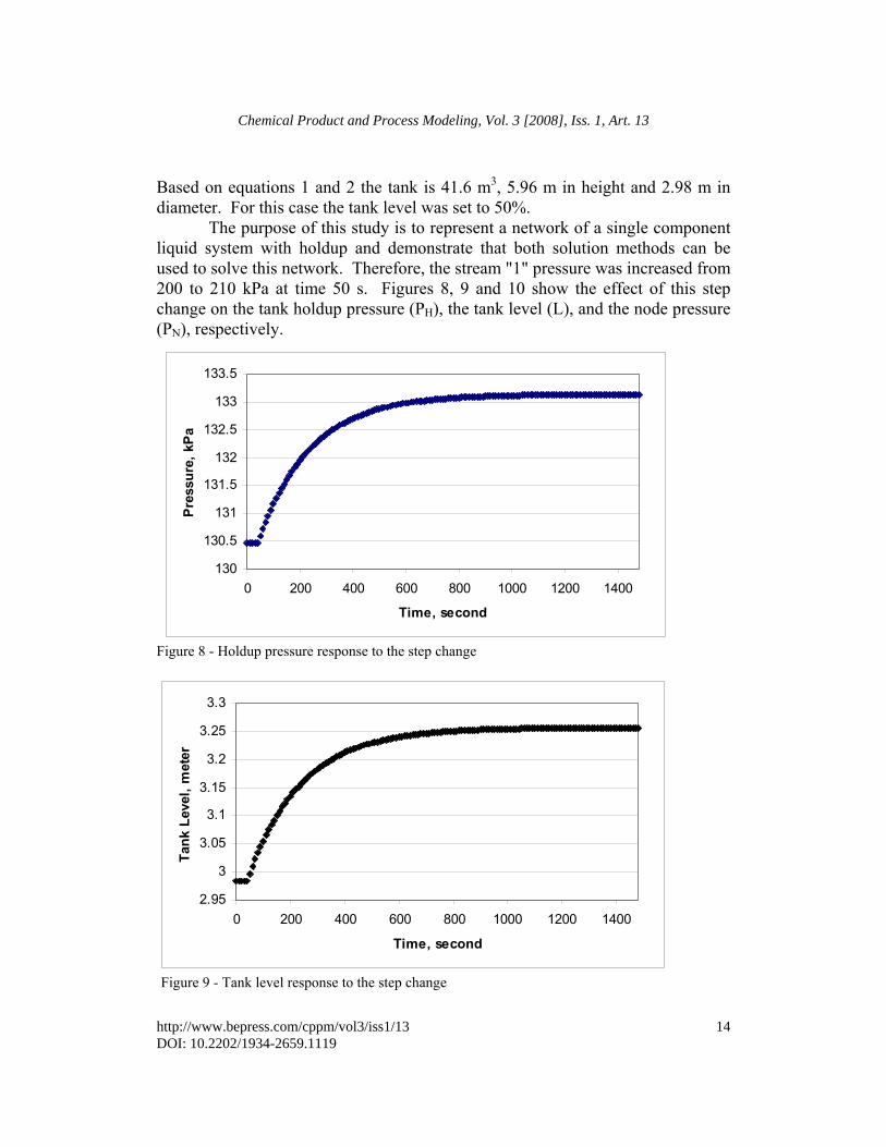
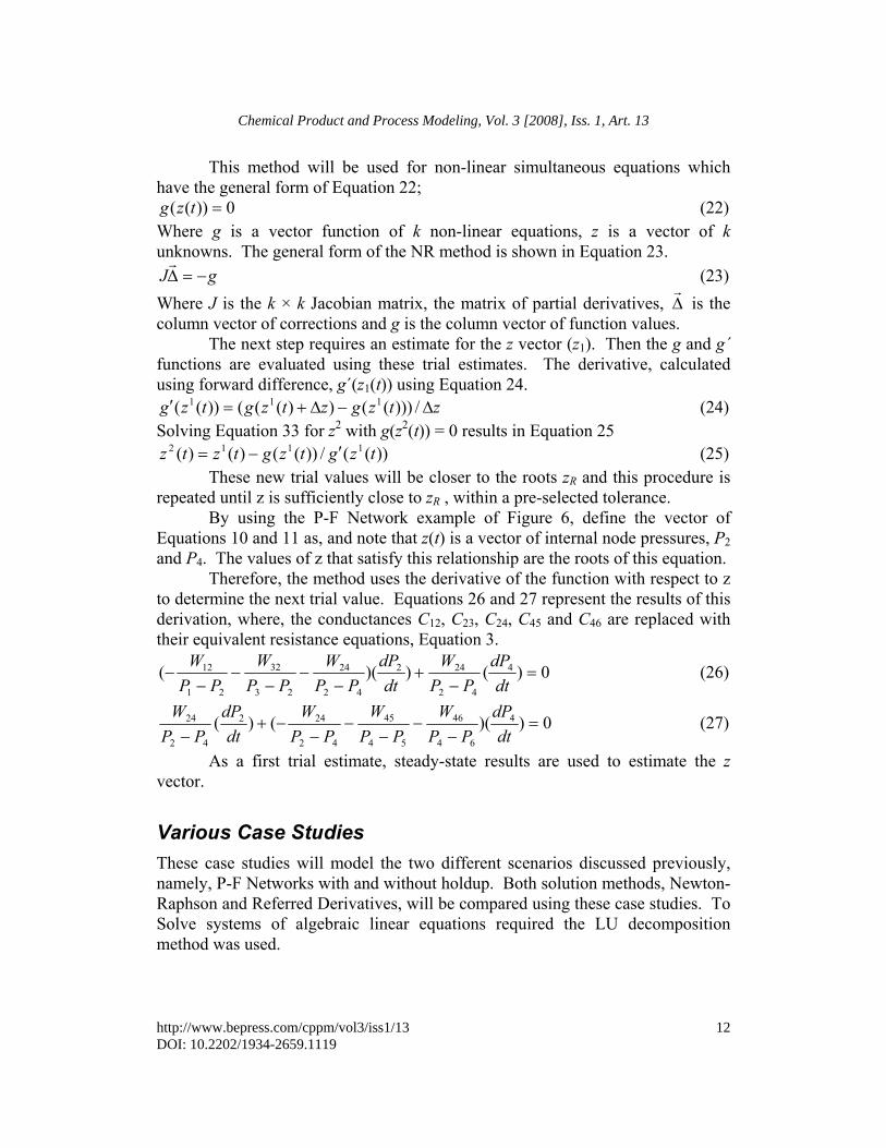
Based on equations 1 and 2 the tank is 41.6 m3, 5.96 m in height and 2.98 m in diameter. For this case the tank level was set to 50%. The purpose of this study is to represent a network of a single component liquid system with holdup and demonstrate that both solution methods can be used to solve this network. Therefore, the stream "1" pressure was increased from 200 to 210 kPa at time 50 s. Figures 8, 9 and 10 show the effect of this step change on the tank holdup pressure (PH), the tank level (L), and the node pressure (PN), respectively.

130

130.5

131

131.5

132

132.5

133

133.5

0 200 400 600 800 1000 1200 1400

Time, second

Pres

sure

, kPa

Figure 8 - Holdup pressure response to the step change

2.95

3

3.05

3.1

3.15

3.2

3.25

3.3

0 200 400 600 800 1000 1200 1400

Time, second

Tank

Lev

el, m

eter

Figure 9 - Tank level response to the step change

14



109.9

110

110.1

110.2

110.3

110.4

110.5

110.6

0 200 400 600 800 1000 1200 1400

Time, second

Pres

sure

, kPa

Figure 10 - Node pressure, PN, response to the step change

The Newton-Raphson and the Referred Derivatives methods were both able to solve the network for the pressure disturbance introduced into stream 1. These results were validated by manual calculations for the first three iterations and also for the final steady-state values. A comparison between the NR and RD methods showed an "exact" match, Figure 11. Both solvers were able to solve this case in approximately 40 seconds. The RD solver took 38 s and the NR solver took 40 s, which is some 37 times faster than the real time. Therefore, one may conclude that both solvers are fast enough to be used within a dynamic simulator.

2.9

2.95

3

3.05

3.1

3.15

3.2

3.25

3.3

2.9 2.95 3 3.05 3.1 3.15 3.2 3.25 3.3

NR Tank Level, m

RD T

ank

Leve

, m

Figure 11 - A comparison between the RD and the NR methods

15



A Binary Mixture Gas System with Holdup Figure 12 is a network that includes four valves, one mixer and one closed tank for a single component gas system with holdup (closed tank), or, re-stated this flowsheet represents a P-F Network with a gas system with holdup. For this case study an equimolar mixture of Ethane and Propane with flowrate of 40000 kg/hr at 20 °C and 1000 kPa was specified in stream 1. The steady-state data are presented in Table 3. Based on the Equations 1 and 2 the tank volume is 58.3 m3.

VLV

3

Figure 12 - Schematic of a Gas System with Holdup Table 3 - Steady-State data P1 1300 kPa F1 40000 kg/hr

P2 1200 kPa F2 40000 kg/hr

P3 1200 kPa F3 40000 kg/hr

P4 1100 kPa F4 40000 kg/hr

P5 1300 kPa F5 5000 kg/hr

P6 1100 kPa F6 45000 kg/hr

P7 1100 kPa F7 45000 kg/hr

P8 1050 kPa F8 45000 kg/hr

Once again a step change increase to stream 1 pressure of 5% from 1300

to 1365 kPa at time 50 s was used as the disturbance. Figures 13, 14 and 15 show the effect of this step change on the tank holdup pressure (PH), the tank inlet and

16



outlet flow rates, and the node pressure (PN), respectively. This case study demonstrates that both solvers, the RD and NR, are capable of solving a P-F Network with a binary mixture gas system with holdup at almost same speed (about 10 s) and provide the same calculation results. Since the property package is the part dealing with flash calculation adding more components to the system fluid is possible.

11951200120512101215122012251230123512401245

0 50 100 150 200 250 300 350

Time, second

Pres

sure

, kP

a

Figure 13 - Holdup pressure response to the step change

30000

35000

40000

45000

50000

55000

0 50 100 150 200 250 300 350

Time, second

Flow

Rat

e, k

g/hr

Tank Inlet Tank Outlet

Figure 14 - Tank inlet and outlet flow rate responses to the step change

17



1098

1100

1102

1104

1106

1108

1110

1112

0 50 100 150 200 250 300 350

Time, second

Pres

sure

, kP

a

Figure 15 - Node pressure, PN, response to the step change

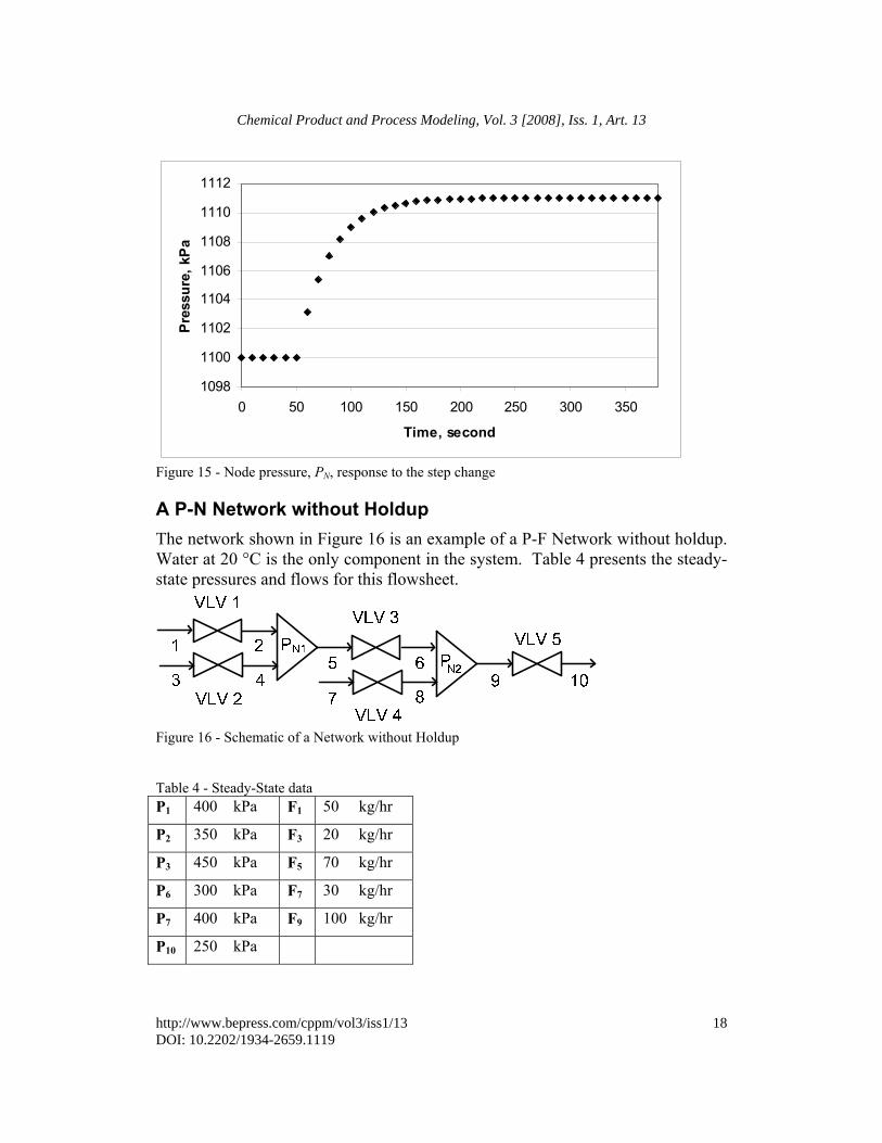
A P-N Network without Holdup The network shown in Figure 16 is an example of a P-F Network without holdup. Water at 20 °C is the only component in the system. Table 4 presents the steady-state pressures and flows for this flowsheet.

Figure 16 - Schematic of a Network without Holdup Table 4 - Steady-State data P1 400 kPa F1 50 kg/hr

P2 350 kPa F3 20 kg/hr



P7 400 kPa F9 100 kg/hr

P10 250 kPa

18



To provide a more demanding test of the P-F Solver for both methods a sinusoidal function with a 5% of steady-state amplitude value and a 10 minute period was used as the disturbance in P1. Figure 17 shows the response of the two internal node pressures (PN1 and PN2) to this disturbance. The top plot shows the pressure change for P1, while the middle plot shows the first node pressure, PN1, resulting from the effect of the disturbance in P1. The bottom plot shows the pressure of the second node, PN2. Figure 18 presents the flow rate changes in the network. Since there is no holdup in the system, all these responses have the same period and relative steady-state amplitude values as the sinusoidal input disturbance that was applied to P1.

270

290

310

330

350

370

390

410

430

0 1000 2000 3000 4000 5000 6000

Time, second

Pres

sure

, kPa

Inlet Node One Node Two

Figure 17 - Pressure responses to the sinusoidal disturbance

19



0

20

40

60

80

100

120

0 1000 2000 3000 4000 5000 6000

Time, second

Flow

Rat

e, m

3/hr

Valve 1 Valve 2 Valve 4 Valve 5

Figure 18 - Flow rate responses to the sinusoidal disturbance Figure 19 is a comparison between the pressures calculated for the PN1 node, using each of the two methods. Again, there would appear to be little or no difference in the numerical results. Both methods solved this case in around 2 min and 45 sec which is 36 faster than real-time.

330

335

340

345

350

355

360

365

370

330 335 340 345 350 355 360 365 370

RD First Node Pressure, kPa

NR

Firs

t Nod

e Pr

essu

re, k

Pa

Figure 19 - A comparison between the RD and the NR methods

20



Comparisons between the RD and the NR solvers showed that some of the calculated results using the Referred Derivatives method were different by 0.5% from those using the Newton-Raphson method. These small differences can be attributed to the nonlinearity of the system, time step size and the type of the disturbance function. For instance by adding in a second node to the system the nonlinearity is increased, therefore, the RD method results will not match exactly the Newton-Raphson results. By decreasing the time step from 10 seconds to one second the average error decreases from 0.083% to 0.0085%. The significance, of course, depends on the plant being simulated.

Conclusions The P-F solver plays a vital role in a dynamic process simulator insuring the fidelity, robustness, accuracy and speed of the plant simulation. This study showed that either the RD or NR methods can be used in solving P-F networks. These solvers (RD and NR) are capable of solving any P-F Network for any flowsheet including valves (unit operations using a resistance equation), tanks (unit operations with holdup) and mixers/splitters (pressure nodes). However, these solvers were designed in a way that one could easily expand them to include other unit operations such as pump, heat-exchanger and tower. As discussed in this study, from the P-F Solver point of view, each unit operation either uses a resistance equation, a volume balance or a combination of both. Therefore adding other unit operations will not be difficult. As the case studies showed, both solvers solved the multi-component P-F Network systems with either liquid or gas phases. Both solvers can also be used to solve P-F Networks with different types of P-F specifications such as constant values, step and/or sinusoidal functions. The Referred Derivatives (RD) method takes advantage of the time-marching environment of the dynamic simulation and converts the system of nonlinear simultaneous P-F equations into a linear system of simultaneous algebraic equations. The linear nature of these equations guarantees a solution, provided that the P-F specifications have a physical meaning. Using a numerical method such as a matrix inverse method, LU decomposition or Gaussian elimination, the linear system of equations can be solved each time step (Riggs, 1994). For this study a matrix inverse method was used. This provides fidelity and robustness in the solver. It was shown that the RD solution method is capable of solving the three test cases about 35 times faster than real time even with a non-optimized code. Arguably, this means that the bottleneck is the flash calculation call happening at every single step time. But this ensures that a dynamic simulator using this solver is computationally useful for the dynamic simulation of large processing plants.

21



This study also showed that the Newton-Raphson (NR) solver is able to solve P-F Networks almost as quickly as the RD solver when "good" initial estimates are provided. Therefore, it can be also be used to solve the P-F Network within a dynamic simulator; however, there are some disadvantages to using the NR method. These disadvantages include the requirement for function derivatives and the method may not converge to a solution or may not converge to the right solution. Another problem is that the solution could become oscillatory. There also exists the possibility of error due to a division by zero during the solution procedure. The NR solver uses the same developed procedure (successive substitution method) as the RD method for solving networks with holdups.

References Bequette, B. W. (1998). Process dynamic modeling, analysis, and simulation,

Prentice Hall PTR, New Jersey. Cota, R. C. (2003). "Development of an open source chemical process simulator",

University of Calgary, Calgary. ISA-The Instrumentation, System, and Automation Society. (2005). Flow

Equations for Sizing Control Valves, ISA, North Carolina. Luyben, W. L. (2002) Plantwide Dynamic Simulators in Chemical Processing

and Control, Marcel Dekker Inc, New York Luyben, W. L. (1989). Process Modeling, Simulation and Control for Chemical

Engineers, McGraw-Hill, Inc. Riggs, J. B. (1994). An introduction to numerical methods for chemical

engineering, Texas Tech University Press, Texas. Seider, W. D., Seader, J. D., and Lewin, D. R. (1998). Process Design Principles:

synthesis, analysis, and evaluation, John Wiley & Sons, Inc., Toronto. Svrcek, W. Y., Mahoney, D. P., and Young, B. R. (2000). A real-time approach

to process control, John Willey & Sons, Ltd, toronto. Thomas, P. (1999). Simulation of Industrial Processes, Butterworth-Heinemann,

Woburn, MA. Thomas, P. J. (1997). "The Method of Referred Derivatives: a New Technique for

Solving Implicit Equations in Dynamic Simulation" Transactions of the Institute of Measurement and Control, 19, 13-21.

Virtual Materials Group. (2006). " VMGThermo", VMG, Calgary, Alberta.

22



chemical product and process modeling - researchspace home

Documents