CHEE 321: Chemical Reaction Engineering

Module ∞: Fun Stuff we didn’t cover

and thinking about the exam

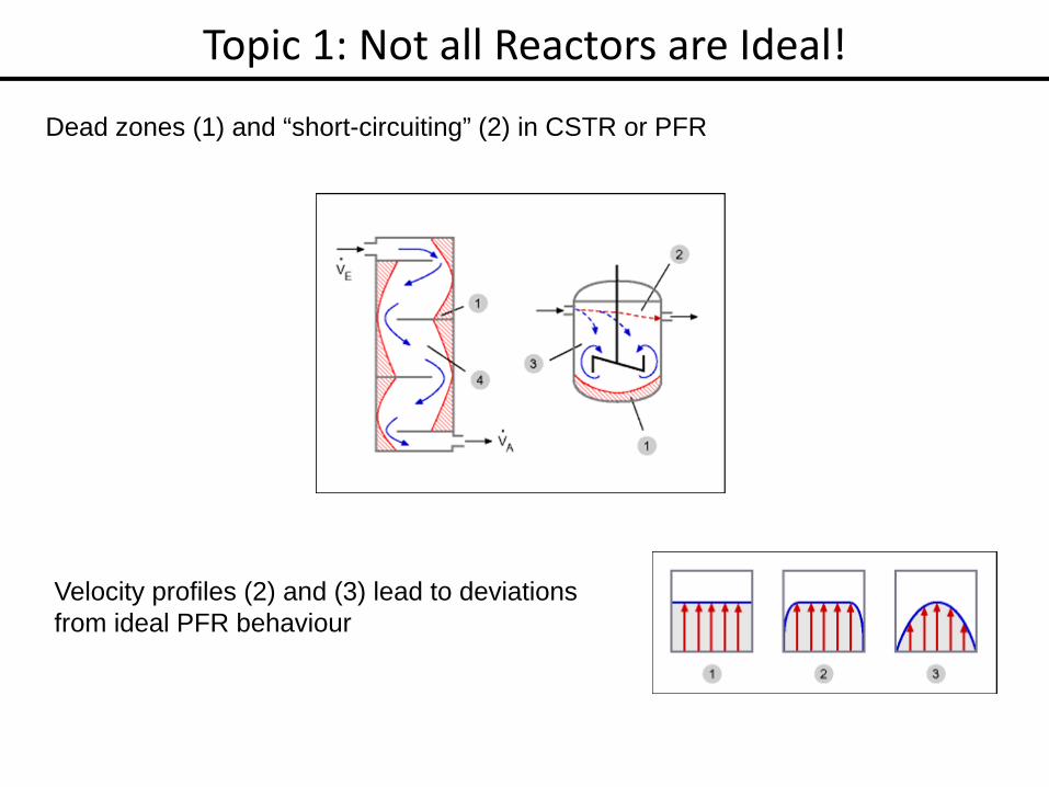
Dead zones (1) and “short-circuiting” (2) in CSTR or PFR

Topic 1: Not all Reactors are Ideal!

Velocity profiles (2) and (3) lead to deviations from ideal PFR behaviour

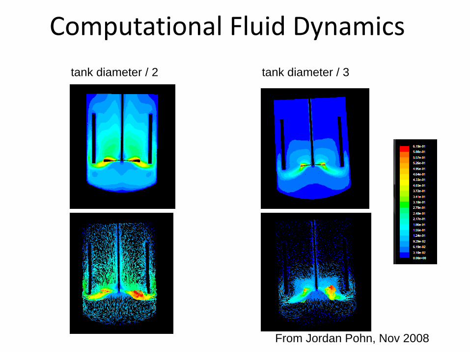
Computational Fluid Dynamicstank diameter / 3tank diameter / 2

From Jordan Pohn, Nov 2008

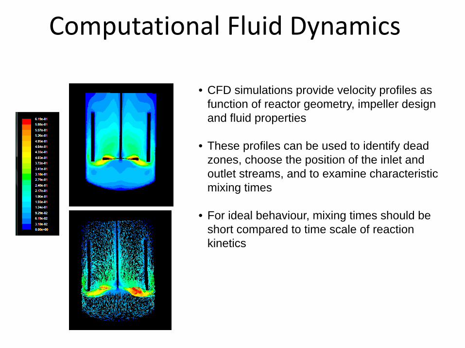
Computational Fluid Dynamics

• CFD simulations provide velocity profiles as function of reactor geometry, impeller design and fluid properties

• These profiles can be used to identify dead zones, choose the position of the inlet and outlet streams, and to examine characteristic mixing times

• For ideal behaviour, mixing times should be short compared to time scale of reaction kinetics

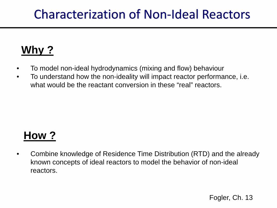
Characterization of Non‐Ideal Reactors

Why ?• To model non-ideal hydrodynamics (mixing and flow) behaviour• To understand how the non-ideality will impact reactor performance, i.e.

what would be the reactant conversion in these “real” reactors.

• Combine knowledge of Residence Time Distribution (RTD) and the already known concepts of ideal reactors to model the behavior of non-ideal reactors.

How ?

Fogler, Ch. 13

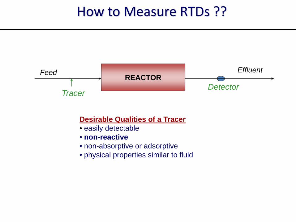
How to Measure RTDs ??

REACTORDetector

Tracer

Feed Effluent

Desirable Qualities of a Tracer• easily detectable• non-reactive• non-absorptive or adsorptive• physical properties similar to fluid

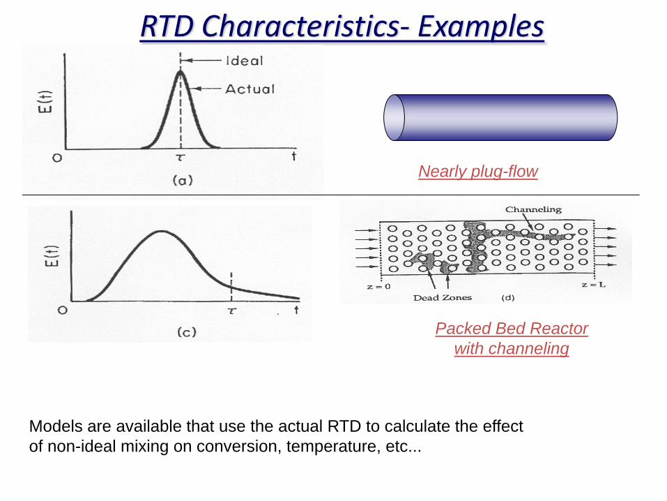
RTD Characteristics‐ Examples

Nearly plug-flow

Packed Bed Reactorwith channeling

Models are available that use the actual RTD to calculate the effectof non-ideal mixing on conversion, temperature, etc...

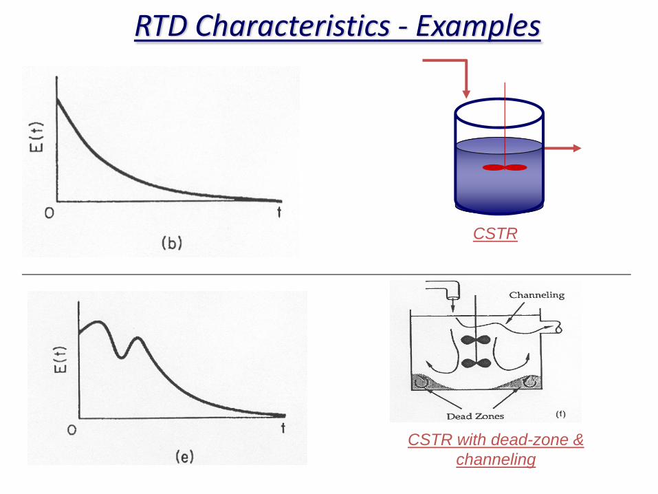
RTD Characteristics ‐ Examples

CSTR

CSTR with dead-zone & channeling

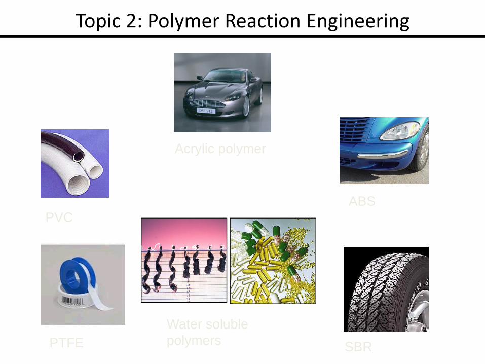
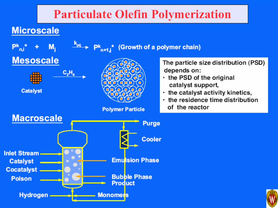
Topic 2: Polymer Reaction Engineering

Acrylic polymer

SBR

ABS

PTFE

PVC

Water soluble polymers

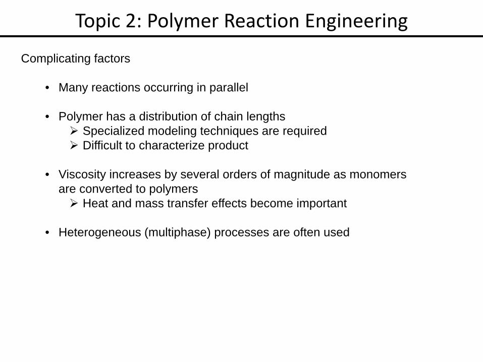
Complicating factors

• Many reactions occurring in parallel

• Polymer has a distribution of chain lengthsSpecialized modeling techniques are requiredDifficult to characterize product

• Viscosity increases by several orders of magnitude as monomers are converted to polymers

Heat and mass transfer effects become important

• Heterogeneous (multiphase) processes are often used

Topic 2: Polymer Reaction Engineering

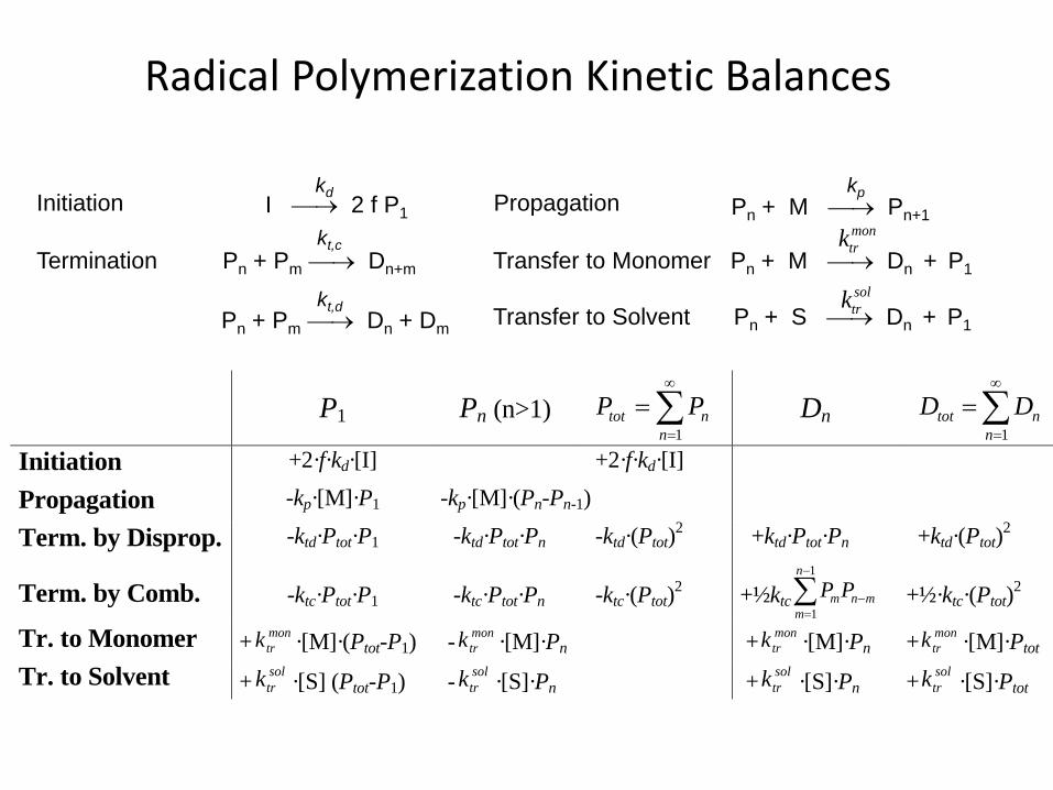
Radical Polymerization Kinetic Balances

Transfer to Monomer Pn + M ⎯→ Dn + P1

Transfer to Solvent Pn + S ⎯→ Dn + P1

Propagation Pn + M ⎯→ Pn+1

Termination Pn + Pm ⎯→ Dn+m

Pn + Pm ⎯→ Dn + Dm

Initiation I ⎯→ 2 f P1

kd kp

kt,c

kt,d

montrk

soltrk

P1 Pn (n>1) ∑∞

=

=1n

ntot PP Dn ∑∞

=

=1n

ntot DD

Initiation +2·f·kd·[I] +2·f·kd·[I]

Propagation -kp·[M]·P1 -kp·[M]·(Pn-Pn-1)

Term. by Disprop. -ktd·Ptot·P1 -ktd·Ptot·Pn -ktd·(Ptot)2 +ktd·Ptot·Pn +ktd·(Ptot)2

Term. by Comb. -ktc·Ptot·P1 -ktc·Ptot·Pn -ktc·(Ptot)2 +½ktc mn

n

mmPP −

−

=∑

1

1+½·ktc·(Ptot)2

Tr. to Monomer + montrk ·[M]·(Ptot-P1) - mon

trk ·[M]·Pn + montrk ·[M]·Pn + mon

trk ·[M]·Ptot

Tr. to Solvent + soltrk ·[S] (Ptot-P1) - sol

trk ·[S]·Pn + soltrk ·[S]·Pn + sol

trk ·[S]·Ptot

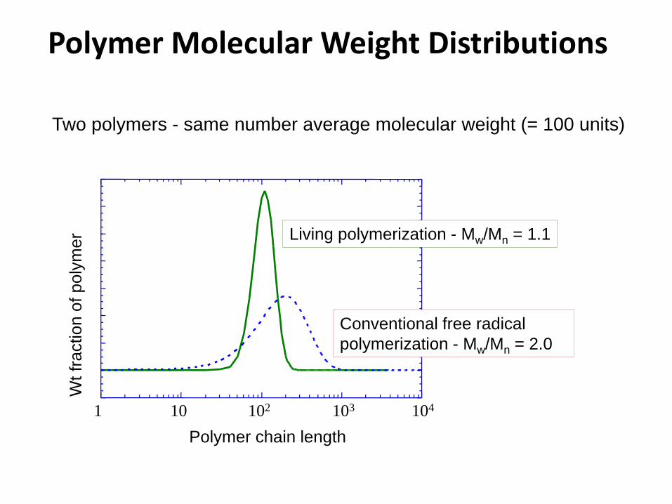
Polymer Molecular Weight Distributions

Living polymerization - Mw/Mn = 1.1

Conventional free radical polymerization - Mw/Mn = 2.0

Two polymers - same number average molecular weight (= 100 units)

1 10 102 103 104

Polymer chain length

Wt f

ract

ion

of p

olym

er

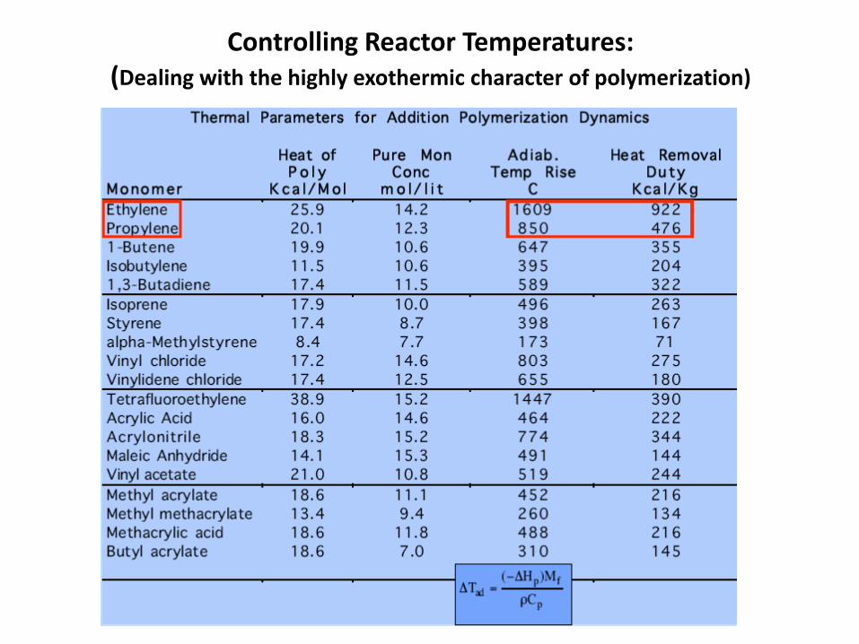
Controlling Reactor Temperatures: (Dealing with the highly exothermic character of polymerization)

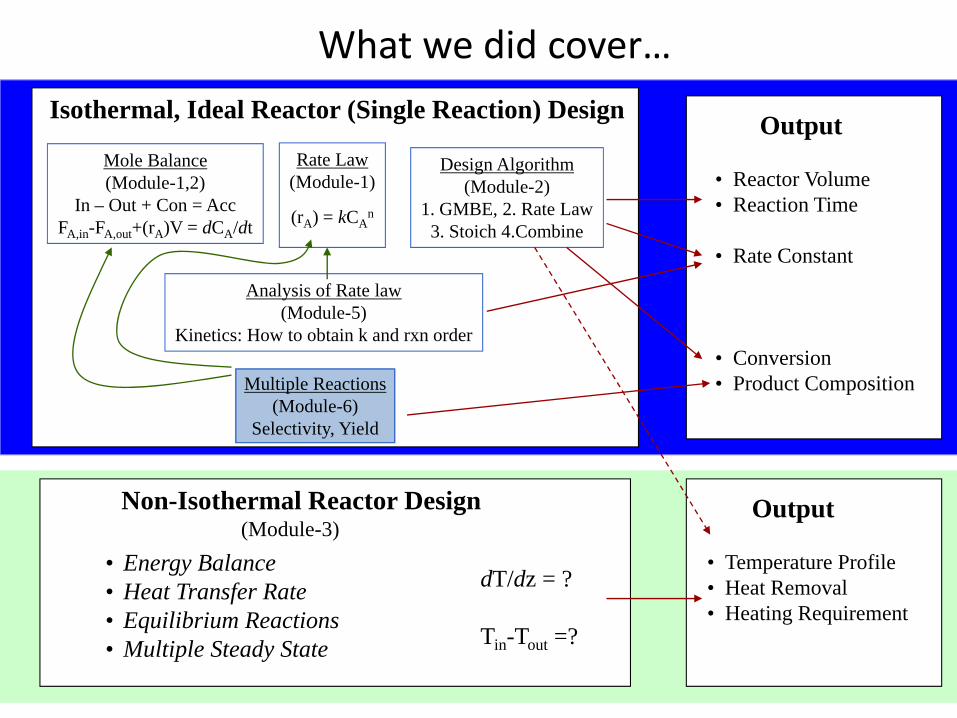
What we did cover…Isothermal, Ideal Reactor (Single Reaction) Design

Mole Balance(Module-1,2)

In – Out + Con = AccFA,in-FA,out+(rA)V = dCA/dt

Rate Law(Module-1)

(rA) = kCAn

Design Algorithm(Module-2)

1. GMBE, 2. Rate Law3. Stoich 4.Combine

Analysis of Rate law(Module-5)

Kinetics: How to obtain k and rxn order

Multiple Reactions(Module-6)

Selectivity, Yield

Non-Isothermal Reactor Design

dT/dz = ?

Tin-Tout =?

Output

• Reactor Volume• Reaction Time

• Rate Constant

• Conversion• Product Composition

• Energy Balance• Heat Transfer Rate• Equilibrium Reactions• Multiple Steady State

(Module-3)• Temperature Profile• Heat Removal• Heating Requirement

Output

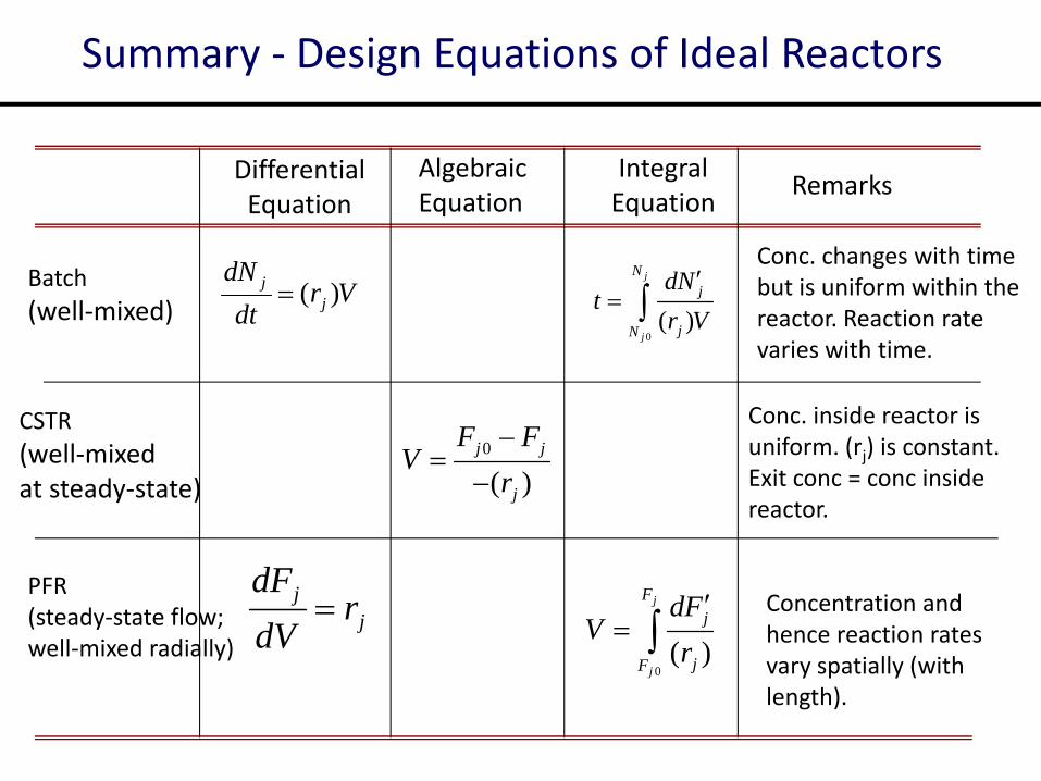
Summary ‐ Design Equations of Ideal Reactors

DifferentialEquation

AlgebraicEquation

IntegralEquation

Remarks

Vrdt

dNj

j )(=0( )

j

j

Nj

jN

dNt

r V′

= ∫Conc. changes with time but is uniform within the reactor. Reaction rate varies with time.

Batch(well‐mixed)

CSTR(well‐mixed at steady‐state)

0

( )j j

j

F FV

r−

=−

Conc. inside reactor is uniform. (rj) is constant. Exit conc = conc inside reactor.

PFR(steady‐state flow; well‐mixed radially)

jj r

dVdF

=

0( )

j

j

Fj

jF

dFV

r′

= ∫Concentration and hence reaction rates vary spatially (with length).

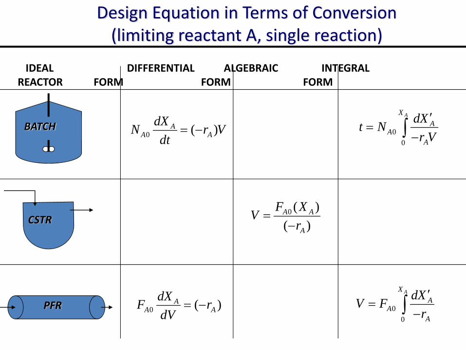
Design Equation in Terms of Conversion(limiting reactant A, single reaction)

IDEAL DIFFERENTIAL           ALGEBRAIC INTEGRAL      REACTOR FORM                             FORM                           FORM

0 ( )AA A

dXN r Vdt

= − 00

AXA

AA

dXt Nr V

′=

−∫

0 ( )AA A

dXF rdV

= − 00

AXA

AA

dXV Fr

′=

−∫

CSTR

PFR

0 ( )( )A A

A

F XVr

=−

BATCH

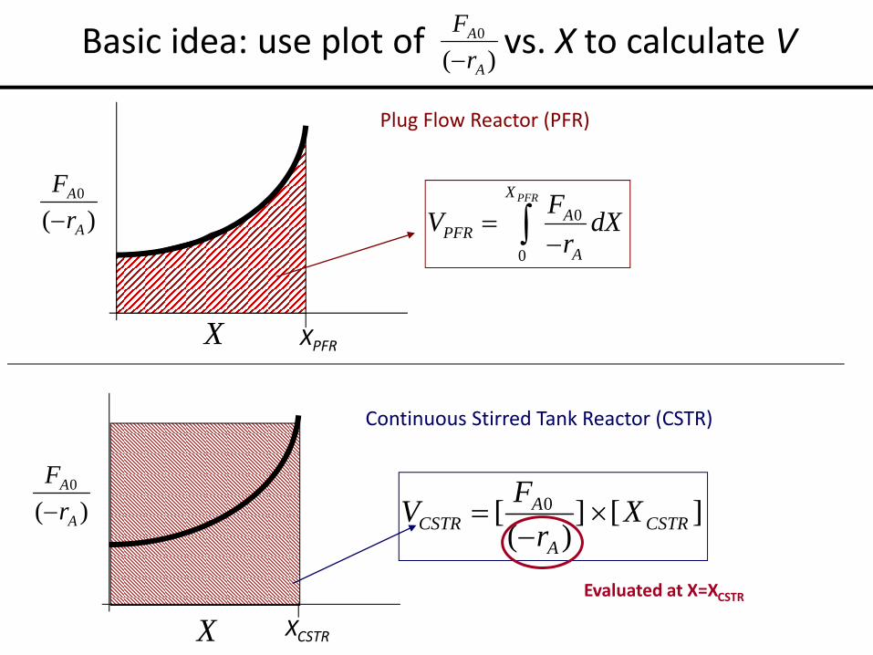
Basic idea: use plot of         vs. X to calculate V

0

0

PFRXA

PFRA

FV dXr

=−∫

X

)(0

A

A

rF−

][])(

[ 0CSTR

A

ACSTR X

rFV ×−

=

Plug Flow Reactor (PFR)

Continuous Stirred Tank Reactor (CSTR)

)(0

A

A

rF−

XEvaluated at X=XCSTR

XPFR

XCSTR

)(0

A

A

rF−

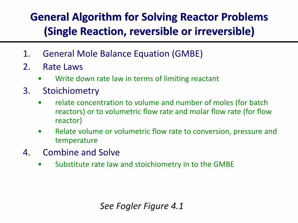
General Algorithm for Solving Reactor Problems (Single Reaction, reversible or irreversible)

1. General Mole Balance Equation (GMBE)2. Rate Laws

• Write down rate law in terms of limiting reactant

3. Stoichiometry• relate concentration to volume and number of moles (for batch 

reactors) or to volumetric flow rate and molar flow rate (for flow reactor)

• Relate volume or volumetric flow rate to conversion, pressure and temperature

4. Combine and Solve• Substitute rate law and stoichiometry in to the GMBE

See Fogler Figure 4.1

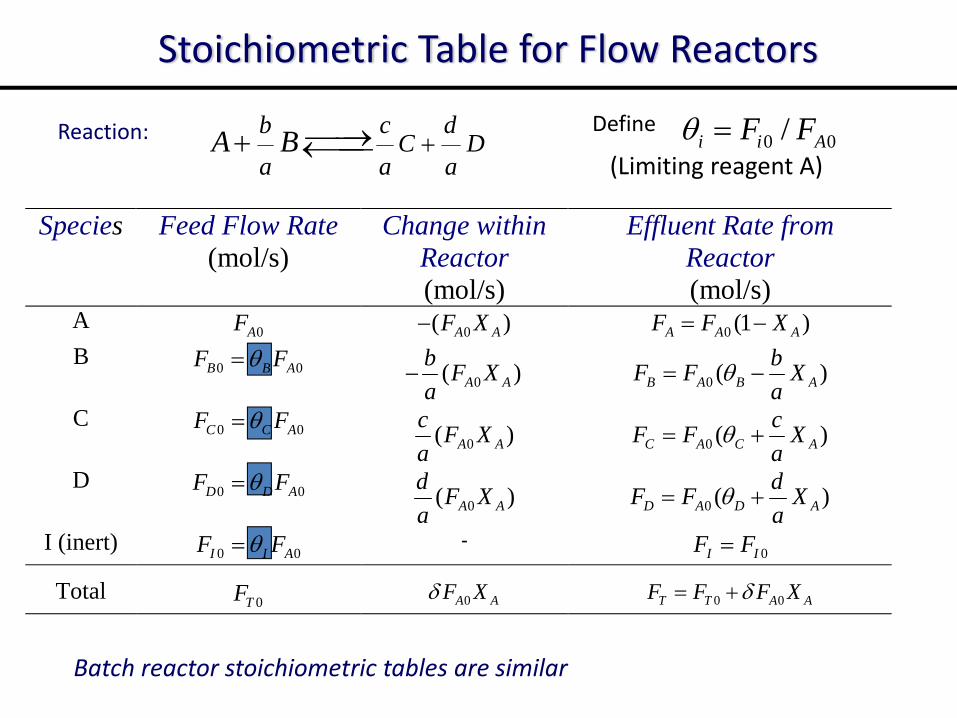
Stoichiometric Table for Flow Reactors

Reaction: b c dC D

a a aA B +⎯⎯→+ ←⎯⎯

Species Feed Flow Rate (mol/s)

Change within Reactor (mol/s)

Effluent Rate from Reactor (mol/s)

A 0AF 0( )A AF X− 0 (1 )A A AF F X= −

B 0 0B B AF Fθ= 0( )A A

b F Xa

− 0 ( )B A B AbF F Xa

θ= −

C 0 0C C AF Fθ= 0( )A A

c F Xa

0 ( )C A C AcF F Xa

θ= +

D 0 0D D AF Fθ= 0( )A A

d F Xa

0 ( )D A D AdF F Xa

θ= +

I (inert) 0 0I I AF Fθ= - 0I IF F=

Total 0TF 0A AF Xδ 0 0T T A AF F F Xδ= +

Batch reactor stoichiometric tables are similar

Define 0 0/i i AF Fθ =

(Limiting reagent A)

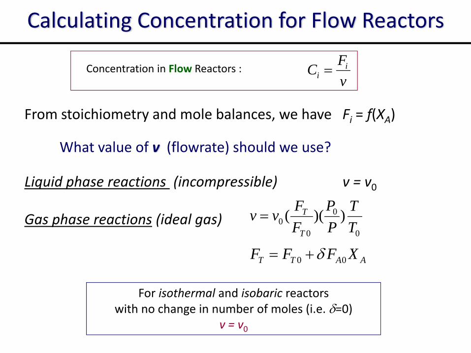
Calculating Concentration for Flow Reactors

From stoichiometry and mole balances, we have   Fi = f(XA)

What value of v (flowrate) should we use?

Liquid phase reactions  (incompressible) v = v0

Gas phase reactions (ideal gas)0

00 0

( )( )T

T

PF Tv vF P T

=

For isothermal and isobaric reactorswith no change in number of moles (i.e. δ=0)

v = v0

Concentration in Flow Reactors : ii

FCv

=

0 0T T A AF F F Xδ= +

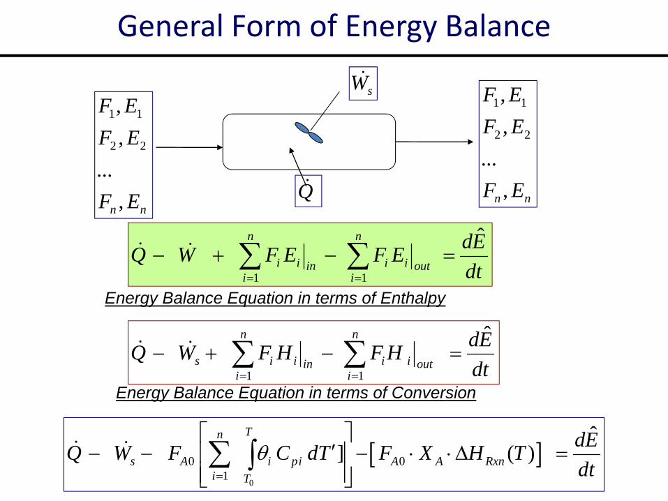
General Form of Energy Balance

dtEdEFEFWQ

outi

n

iiini

n

ii

ˆ

11=−+− ∑∑

==

sW

Qnn EF

EFEF

,...

,,

22

11

nn EF

EFEF

,...

,,

22

11

dtEdHFHFWQ

outi

n

iiini

n

iis

ˆ

11=−+− ∑∑

==

Energy Balance Equation in terms of Enthalpy

[ ]0

0 01

ˆ] ( )

Tn

s A i pi A A Rxni T

dEQ W F C dT F X H Tdt

θ=

⎡ ⎤′− − − ⋅ ⋅ Δ =⎢ ⎥

⎢ ⎥⎣ ⎦∑ ∫

Energy Balance Equation in terms of Conversion

010

( ) ( ) ( ) ( )n

aRxn ref p ref A i pi

iA

UA T T H T C T T X C T TF

θ=

− ⎡ ⎤− Δ + Δ − ⋅ = −⎣ ⎦ ∑

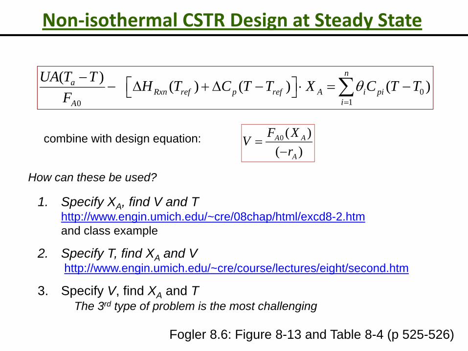
Non‐isothermal CSTR Design at Steady State

Fogler 8.6: Figure 8-13 and Table 8-4 (p 525-526)

combine with design equation: 0 ( )( )A A

A

F XVr

=−

How can these be used?

1. Specify XA, find V and Thttp://www.engin.umich.edu/~cre/08chap/html/excd8-2.htmand class example

2. Specify T, find XA and Vhttp://www.engin.umich.edu/~cre/course/lectures/eight/second.htm

3. Specify V, find XA and TThe 3rd type of problem is the most challenging

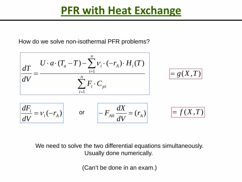
PFR with Heat Exchange

1

1

( ) ( ) ( )n

a i A ii

n

i pii

U a T T r H TdTdV F C

ν=

=

⋅ ⋅ − − ⋅ − ⋅=

⋅

∑

∑

How do we solve non-isothermal PFR problems?

)( Aii r

dVdF

−=ν )(0 AA rdVdXF =−or ),( TXf=

),( TXg=

We need to solve the two differential equations simultaneously.Usually done numerically.

(Can’t be done in an exam.)

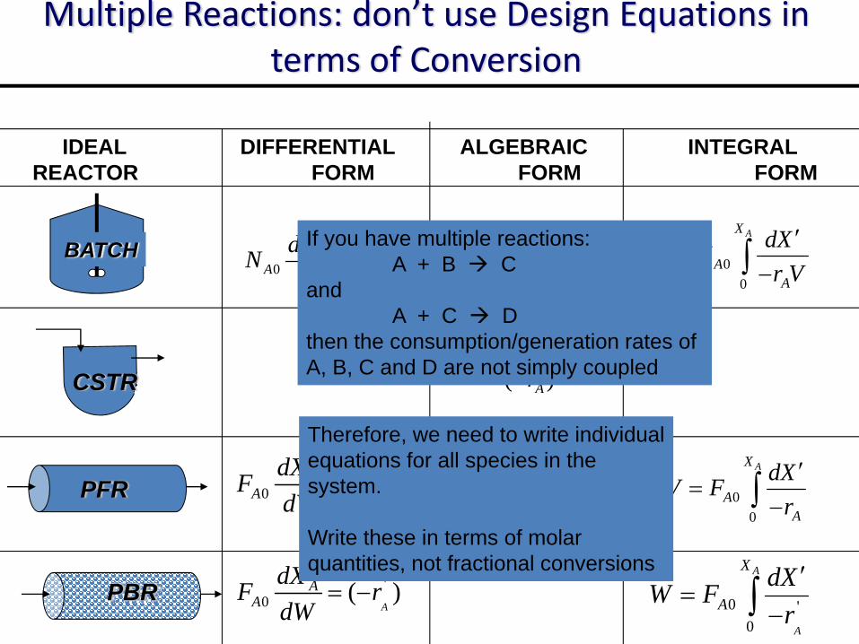
Multiple Reactions: don’t use Design Equations in terms of Conversion

'0 ( )

A

AA

dXF rdW

= −

IDEAL DIFFERENTIAL ALGEBRAIC INTEGRAL REACTOR FORM FORM FORM

0 ( )AA A

dXN r Vdt

= − 00

AX

AA

dXt Nr V

′=

−∫

0 ( )AA A

dXF rdV

= −0

0

AX

AA

dXV Fr

′=

−∫

CSTR0 ( )

( )A A

A

F XVr

=−

BATCH

PFR

PBR 0 '0

A

A

X

AdXW F

r′

=−∫

If you have multiple reactions:A + B C

andA + C D

then the consumption/generation rates of A, B, C and D are not simply coupled

Therefore, we need to write individual equations for all species in the system.

Write these in terms of molar quantities, not fractional conversions

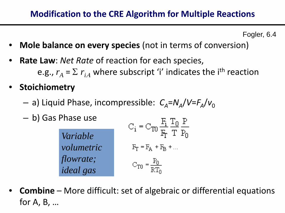
Modification to the CRE Algorithm for Multiple Reactions

• Mole balance on every species (not in terms of conversion)

• Rate Law: Net Rate of reaction for each species, e.g., rA = Σ riΑ where subscript ‘i’ indicates the ith reaction

• Stoichiometry

– a) Liquid Phase, incompressible:  CA=NA/V=FA/v0– b) Gas Phase use 

• Combine – More difficult: set of algebraic or differential equations for A, B, …

Fogler, 6.4

Variable volumetric flowrate; ideal gas

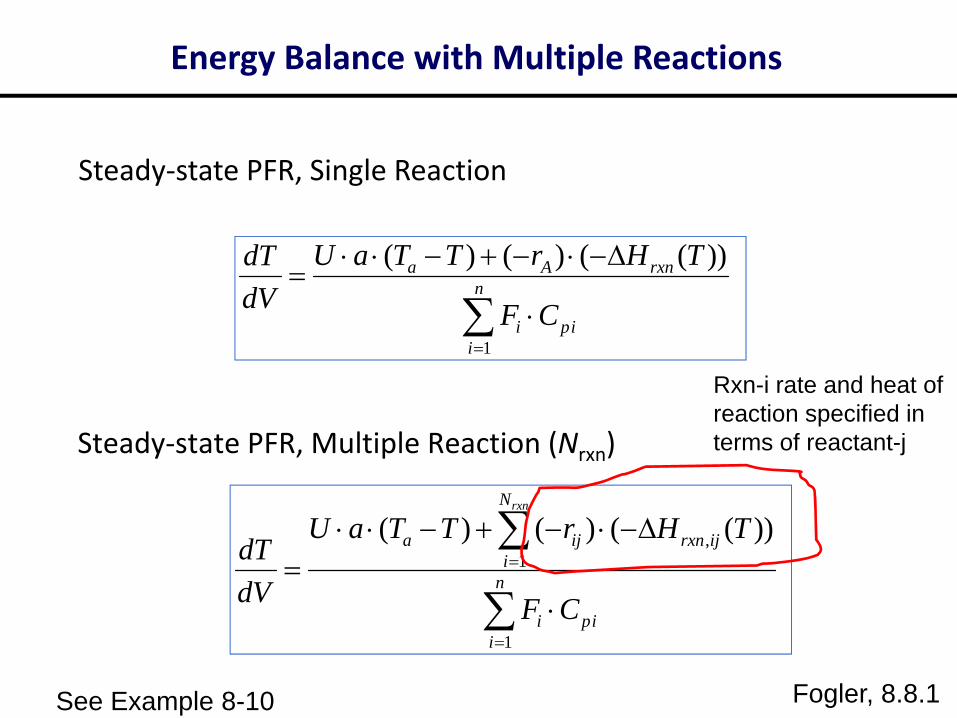
Energy Balance with Multiple Reactions

Steady‐state PFR, Single Reaction

1

( ) ( ) ( ( ))a A rxnn

i pii

U a T T r H TdTdV F C

=

⋅ ⋅ − + − ⋅ −Δ=

⋅∑

Steady‐state PFR, Multiple Reaction (Nrxn)

,1

1

( ) ( ) ( ( ))rxnN

a ij rxn iji

n

i pii

U a T T r H TdTdV F C

=

=

⋅ ⋅ − + − ⋅ −Δ=

⋅

∑

∑

Fogler, 8.8.1

Rxn-i rate and heat of reaction specified in terms of reactant-j

See Example 8-10

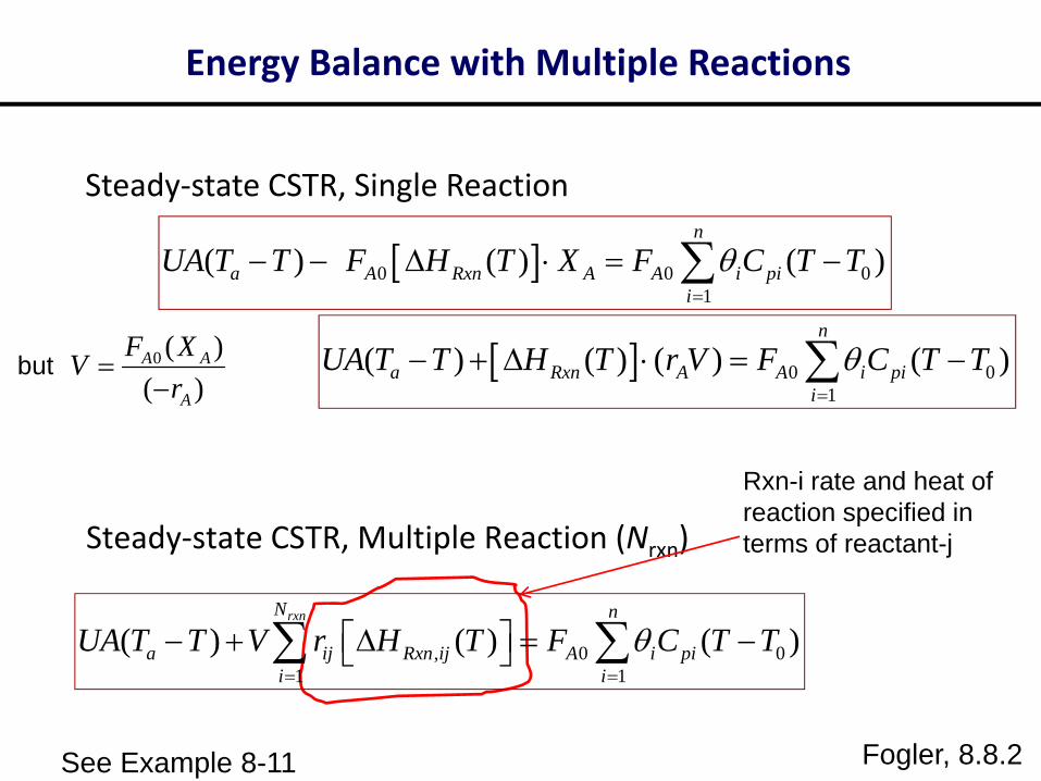
Energy Balance with Multiple Reactions

Steady‐state CSTR, Single Reaction

Steady‐state CSTR, Multiple Reaction (Nrxn)

Fogler, 8.8.2

Rxn-i rate and heat of reaction specified in terms of reactant-j

See Example 8-11

[ ]0 0 01

( ) ( ) ( )n

a A Rxn A A i pii

UA T T F H T X F C T Tθ=

− − Δ ⋅ = −∑

[ ] 0 01

( ) ( ) ( ) ( )n

a Rxn A A i pii

UA T T H T r V F C T Tθ=

− + Δ ⋅ = −∑0 ( )( )A A

A

F XVr

=−

but

, 0 01 1

( ) ( ) ( )rxnN n

a ij Rxn ij A i pii i

UA T T V r H T F C T Tθ= =

⎡ ⎤− + Δ = −⎣ ⎦∑ ∑

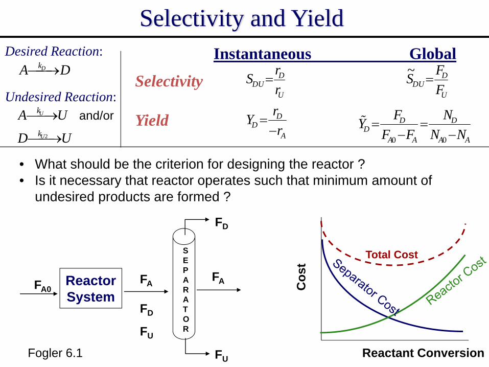
Selectivity and YieldInstantaneous Global

U

DDU r

rS =U

DDU F

FS =~

A

DD r

rY−

=0 0

D DD

A A A A

F NYF F N N

= =− −

Selectivity

Yield

• What should be the criterion for designing the reactor ? • Is it necessary that reactor operates such that minimum amount of

undesired products are formed ?

Total Cost

Desired Reaction:

Undesired Reaction:

DA Dk⎯→⎯

2

U

U

k

k

A U

D U

⎯⎯→

⎯⎯→

Cos

t

Reactant Conversion

ReactorSystem

FA0FA

FD

FU

FD

FU

SEPARATOR

FA

and/or

Fogler 6.1

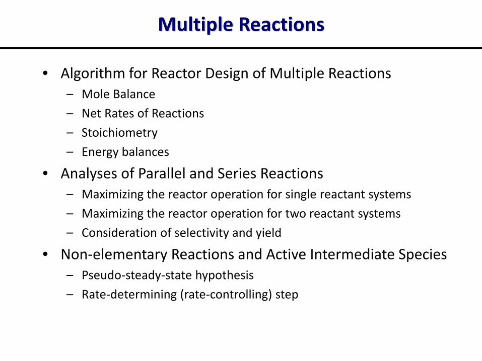
Multiple Reactions

• Algorithm for Reactor Design of Multiple Reactions– Mole Balance

– Net Rates of Reactions

– Stoichiometry

– Energy balances

• Analyses of Parallel and Series Reactions– Maximizing the reactor operation for single reactant systems

– Maximizing the reactor operation for two reactant systems

– Consideration of selectivity and yield

• Non‐elementary Reactions and Active Intermediate Species– Pseudo‐steady‐state hypothesis

– Rate‐determining (rate‐controlling) step 

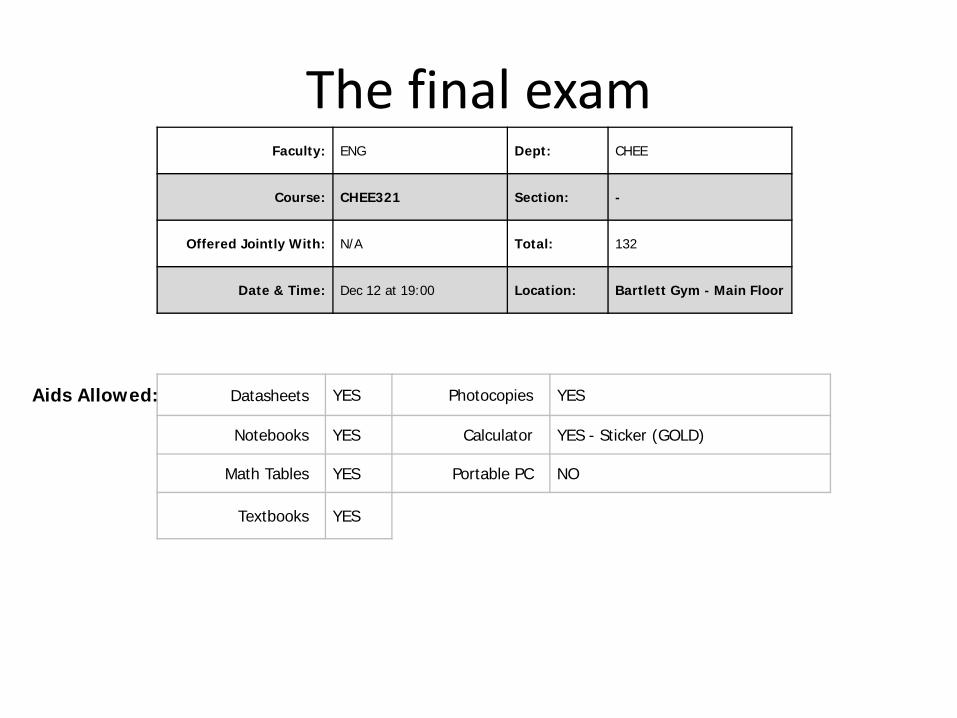
The final examFaculty: ENG Dept: CHEE

Course: CHEE321 Section: -

Offered Jointly With: N/A Total: 132

Date & Time: Dec 12 at 19:00 Location: Bartlett Gym - Main Floor

Datasheets YES Photocopies YES

Notebooks YES Calculator YES - Sticker (GOLD)

Math Tables YES Portable PC NO

Textbooks YES

Aids Allowed:

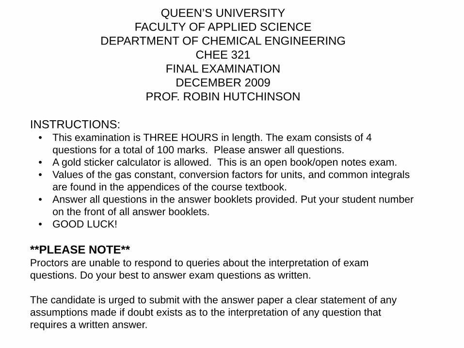
QUEEN’S UNIVERSITYFACULTY OF APPLIED SCIENCE

DEPARTMENT OF CHEMICAL ENGINEERINGCHEE 321

FINAL EXAMINATIONDECEMBER 2009

PROF. ROBIN HUTCHINSON

INSTRUCTIONS:• This examination is THREE HOURS in length. The exam consists of 4

questions for a total of 100 marks. Please answer all questions. • A gold sticker calculator is allowed. This is an open book/open notes exam. • Values of the gas constant, conversion factors for units, and common integrals

are found in the appendices of the course textbook.• Answer all questions in the answer booklets provided. Put your student number

on the front of all answer booklets. • GOOD LUCK!

**PLEASE NOTE**Proctors are unable to respond to queries about the interpretation of exam questions. Do your best to answer exam questions as written.

The candidate is urged to submit with the answer paper a clear statement of any assumptions made if doubt exists as to the interpretation of any question that requires a written answer.

Why Design Projects?

This To This

Σ