chemical sensor networks for the aquatic …...chemical sensor networks for the aquatic environment...

Chemical Sensor Networks for the Aquatic Environment

Kenneth S. Johnson,*,† Joseph A. Needoba,† Stephen C. Riser,‡ and William J. Showers§

Monterey Bay Aquarium Research Institute, 7700 Sandholdt Road, Moss Landing, California 95039, School of Oceanography, University ofWashington, Seattle, Washington 98195-7940, Department of Marine, Earth and Atmospheric Sciences, North Carolina State University,

Raleigh, North Carolina 27695

Received July 14, 2006

Contents1. Introduction 623

1.1. The Sampling Problem 6241.2. Data at Global Scales 625

2. In Situ Chemical Sensors and Analyzers 6262.1. Dissolved Gases Other Than CO2 627

2.1.1. Dissolved Oxygen 6272.1.2. Methane and Total Gas Tension 629

2.2. Inorganic Carbon System 6292.2.1. CO2 Partial Pressure (pCO2) 6292.2.2. pH and Other Inorganic Carbon

Properties630

2.3. Nutrients 6302.3.1. Nutrient Analyzers 6302.3.2. Ion Selective Electrodes 6312.3.3. UV Optical Nitrate Sensors 631

2.4. Empirical Sensors 6313. Chemical Sensor Networks 632

3.1. MBARI/NOAA pCO2 Array 6323.2. Trans-Pacific Sections of Dissolved O2

Measured on Argo Profiling Floats632

3.3. The RiverNet System: Monitoring NitrateFlux in Rivers

635

3.4. Land/Ocean Biogeochemical Observatory 6364. Conclusions and Future Prospects 6385. Acknowledgments 6396. References 639

1. IntroductionA recent commentary speaks to a broad range of potential

applications for autonomous chemical sensor networks,including systems that monitor the state of the environmentin real time.1 However, the authors of the commentary notedthat existing sensor networks are “almost entirely restrictedto transducers for detecting physical parameters such astemperature, pressure, light or movement”. They termed thisthe “chemical sensor paradox”, a condition that resultsbecause current technology “makes the realization of small,autonomous, reliable, chemo/bio-sensing devices impracticalat present”.

Rapid strides have been made toward autonomous chemi-cal sensing capabilities in the past decade by the marine and

aquatic chemistry communities. While chemical sensors arenot at the same level of cost or reliability as physical sensors,a variety of chemical sensing systems are now continuouslydeployed in aquatic environments such as rivers, lakes,estuaries, and the open ocean. These chemical sensors arebeing operated, in some cases, for multiyear periods and inthe ocean at thousands of kilometers distance from shore.Data from dozens of sensors are being delivered in near-real time directly to the Internet.

The primary emphasis of this review is focused on suchchemical sensor networks that can be deployed on autono-mous platforms in aquatic environments and then operatedwithout significant human intervention for extended periods.The aquatic sensor networks that we consider have twoessential characteristics: (1) chemical sensors are deployedin situ at multiple locations, and (2) the networks are operatedfor months to years. These observing systems are dedicatedto observing environmental processes in real time. Much ofthis effort is quite recent, and this article serves as anintroduction to this work, as well as a review.

We focus on observing systems that operate for extendedperiods for two primary reasons. Long-term observations ofthe environment are essential to understanding variabilitydriven by natural and anthropogenic climate change. In situsensors also provide the continuous data needed to character-ize high-frequency signals that cannot be easily sampled bymanual methods. Undersampling of time-varying environ-mental processes can result in aliasing of the observed signal.The variability that is driven by processes occurring at higherfrequencies than the sampling frequency of the environmentcan appear as unrecognizable low-energy events.2

Environmental chemists have often avoided the questionsrelated to undersampling time-varying signals by assumingthat aquatic systems are in a steady state. With thisassumption, a single set of observations then provides anadequate assessment of environmental processes. This as-sumption has been necessary because, until recently, nearlyall observations of chemicals in the aquatic environmentrequired that a sample be collected and returned to thelaboratory, where a variety of sophisticated tools could beused for sample analysis.3 Much of the ocean is sampledonly a few times in a decade because of the long (weeks insome cases) transit times from seaports to mid-ocean regions.Even in the coastal ocean, or lakes and rivers, samples forchemical analysis are generally collected only at monthlyintervals, if at all.4 Such sampling rates are often inadequateto characterize the dominant seasonal, daily, or semi-diurnalprocesses, which occur at well-defined frequencies, as wellas episodic events driven by storms or other processes. Eventhe signals of decadal-scale processes may be contaminated

† Monterey Bay Aquarium Research Institute.‡ University of Washington.§ North Carolina State University.

623Chem. Rev. 2007, 107, 623−640

10.1021/cr050354e CCC: $65.00 © 2007 American Chemical SocietyPublished on Web 01/24/2007

by variability that occurs at higher frequency. Interpretationof the linkages between processes is further obscured dueto long-term lags between cause and effect.5 As a result, webegin by arguing that observing the environment requiressustained, high-frequency observations.

1.1. The Sampling Problem

We illustrate the problems that arise in monitoring effortsthat are based on manual sampling by considering nitrate inaquatic systems. Nitrate is the dominant source of fixednitrogen for new plant growth in most aquatic ecosystems.Surface waters in the open ocean are depleted in plant

nutrients, including nitrate. This depletion is a result ofnutrient incorporation by photosynthetic organisms andsubsequent sinking of organic material in fecal pellets anddecaying organic matter. Deep waters are enriched innutrients when heterotrophic organisms remineralize sinkingparticles. The low concentrations of nitrate in the sunlitsurface waters limit the accumulation of plant biomass inmany marine and freshwater systems.6 Processes that addnew nutrients, such as vertical transport (upwelling ordiffusion) of essential nutrients from deep waters into thesunlit euphotic zone or nitrogen fixation, then become therate-limiting step for primary production of new organiccarbon.

Figure 1 shows nitrate measurements made on a mooringlocated 20 km off the central California coast at hourlyintervals for 1 year7 using an optical nitrate sensor8 and nitrate

Ken Johnson was born in Bellingham, Washington. He received B.S.degrees in Chemistry and in Oceanography from the University ofWashington in 1975 and his Ph.D. in Chemical Oceanography from OregonState University in 1979 under the direction of the late Ric Pytkowicz. Hewas a Research Oceanographer at the University of California, SantaBarbara from 1979 to 1988 and Professor of Oceanography at the MossLanding Marine Laboratories from 1988 to 1999, where he also held ajoint appointment as a Senior Scientist at the Monterey Bay AquariumResearch Institute. He moved to MBARI full time in 1999, where he directsthe Chemical Sensor Laboratory. His research interests include develop-ment of novel sensors and analytical methods for trace metals and nutrientsdissolved in sea water and application of these methods to studies ofbiogeochemical cycles in the ocean.

Joe Needoba was born in 1973 in Vancouver, British Columbia, Canada.In 1997 he received a B.Sc. in the Combined Biology and Oceanographyhonors program from the University of British Columbia (UBC). He receiveda Ph.D. from UBC in 2003. His doctorate thesis with Dr. P. J. Harrisonfocused on the processes of natural abundance stable isotope fractionationof nitrogen in the marine nitrogen cycle. In 2004 he started a postdoctoralfellowship at the Monterey Bay Aquarium Research Institute with theChemical Sensor Laboratory led by Dr. K. S. Johnson. This project focuseson the application of the LOBO chemical sensor network to studies ofenvironmental processes.

Stephen C. Riser studied physics, engineering, and oceanography atPurdue University and the Massachusetts Institute of Technology. Hereceived his Ph.D. degree from the Graduate School of Oceanographyat the University of Rhode Island in 1982. Since 1984 he has been at theSchool of Oceanography, University of Washington, in Seattle, Washington,where he is presently Professor of Oceanography. His work concernsthe general circulation of the ocean and its interaction with the atmosphereand the ocean’s role in climate change. He works extensively with marineinstrumentation and new methods of observing the ocean circulation.

Bill Showers was born in St. Paul, Minnesota. He received a Bachelordegree in Geology from University of California, Santa Barbara in 1973,an MS in Geology from University of California, Davis in 1978, and aPh.D. in Geological Oceanography in 1982 from the Hawaii Institute ofGeophysics at the University of Hawaii. He has been a faculty memberin the Department of Marine, Earth, & Atmospheric Sciences at NorthCarolina State University since 1982, where he is also the Director of theNCSU Stable Isotope Lab and the Director of the RiverNet Program. Hisresearch interests include paleoceanography and solar influences onclimate, paleobiology of dinosaurs and flightless birds, groundwaterpollution, and the flux of nitrogen in watersheds.

624 Chemical Reviews, 2007, Vol. 107, No. 2 Johnson et al.

measurements in samples collected near the mooring at∼21day intervals. The annual cycle observed by the mooredchemical sensor shows a series of events throughout the yearwith high (>10µM) nitrate concentrations. These events areproduced by upwelling of cold, nutrient-rich water, whichis driven to the surface when the wind blows to the southeastin this region. Upwelling of cold, nutrient-rich deep waterinto warm, nutrient-poor surface water produces the anti-correlation in temperature and nitrate (Figure 1). Thenutrients carried into sunlit surface waters during theupwelling events result in phytoplankton blooms that increasechlorophyll concentrations and deplete nitrate (Figure 1). Thiscycle of events, clearly seen in the hourly data, is not easilyresolved in monthly monitoring data. A quantitative under-standing of such processes has come from intensive fieldsampling campaigns. However, intensive field programs aredifficult to sustain in the long-term. As a result, most aquaticenvironments are severely undersampled, long-term varia-tions are not understood, and our understanding of environ-mental processes can be quite biased.

In addition to large temporal variability, there is alsosignificant spatial variability in concentrations of chemicalsthat play important roles in regulating ecosystems. Forexample, the physical processes that reintroduce nutrientsto the surface have high spatial variability. This may producegreat spatial variability in the growth of phytoplanktonpopulations. Thus, chemical sensors in this type of environ-ment should, ultimately, be capable of characterizing highspatial variability, as well as temporal variability.

The undersampling problem, which is inherent in mea-surement programs that are based on manual sample col-lection, can be overcome either by using remote samplecollection devices9,10 or by making nearly continuous chemi-cal measurements over long time periods on networks ofunattended platforms. Here we focus on systems that makein situ measurements. Chemical sensors deployed in situ forextended periods have shown the impacts of events drivenby storms,11 eddies,12,13 El Nino climate oscillations,14,15

planetary (Rossby) waves,16 tides,17 upwelling,7 and icemelting.18

1.2. Data at Global ScalesThe need for a better understanding of the linkages

between chemicals and environmental processes is drivenby the globally significant scope of environmental changepresumed to be occurring. During the past 100 years,concentrations of carbon dioxide in the atmosphere haveincreased 36%, industrial and agricultural processes that fixdinitrogen gas have grown to the point where their rates nowexceed natural processes,19 some 10-50% of the photosyn-thetic products on land are appropriated by processescontrolled by humans,20 and one-half of the accessiblefreshwater runoff is already utilized.21 Such global scaleprocesses necessarily require global observing systems.

The best example of the power of a global environmentalchemical analysis network is the system of stations thatcollect atmospheric measurements of carbon dioxide andoxygen. These networks build on the pioneering work ofthe late Charles David Keeling, who started the time seriesof atmospheric carbon dioxide measurements at Mauna Loain Hawaii. Keeling’s CO2 data from Mauna Loa have playeda seminal role in identifying human perturbation of globalchemical cycles, and it has been the most influentialenvironmental data set now available. His results led to anexpansion of the observing system, and there is now anetwork of stations around the world where samples forcarbon dioxide and oxygen are collected.22,23 The networkmeasurements reveal distinct annual cycles in atmosphericoxygen and carbon dioxide concentrations. Further, there isa distinct geographic pattern to the variability that is relatedto differences in land and ocean areas in the Northern andSouthern Hemispheres. The patterns of annual variation aredriven by photosynthesis and respiration on land and in thesea and by differences in the rates at which these twochemicals equilibrate across the air-sea interface. Thesegeographic and temporal variations in chemical propertiesof the atmosphere allow the long-term, network-basedobservations to be used to create estimates of global netprimary production on land and in the ocean and to quantifythe interannual change in these rates.22,23

Ultimately, monitoring aquatic biogeochemical cycles andtheir impacts on the environment and climate will requiredense networks of chemical sensors that operate at globalscales within the oceans, lakes, and rivers, as well as in theatmosphere. While there are no direct examples operatingat a global scale today, there are a variety of in situ chemicalsensor networks operating at smaller scales. Further, thereare examples of global aquatic sensor networks that illustratethe potential for the development of networks that sensechemical properties. For example, we describe in section 3.2chemical sensor measurements from the Argo array ofprofiling floats.24 These platforms have become an importanttool for observing the large-scale ocean circulation. Profilingfloats typically drift passively with the flow at depths of 1000or 2000 m in the ocean and then cycle at 7-10 day intervalsaway from their parking depth by inflation of a bladder,which increases float volume without changing mass. Thiscauses the float to rise. During the ascent to the surface, thefloats collect measurements of oceanic variables such astemperature and salinity at 50-75 different pressure levels.The floats transmit their data to orbiting satellite communica-tion networks while on the surface and then descend backto their parking depth to begin another cycle.

A map of seawater salinity at a depth of 200 m based onin situ salinity measurements that were made by∼1200 Argo

Figure 1. Measurements of temperature (A), nitrate (B), andchlorophyll (C) made at hourly intervals for 1 year on the M1mooring 20 km offshore in Monterey Bay, California. Nitrate wasmeasured with an optical nitrate sensor.8 Chlorophyll concentrationwas calculated from the attenuation of sunlight at 490 nm betweenthe surface and 10 m. Measurements of nitrate and chlorophyll insamples collected near the mooring at approximately 21 dayintervals are shown as open circles. Adapted from ref 7, Copyright2006, with permission from Elsevier.

Chemical Sensor Networks for the Aquatic Environment Chemical Reviews, 2007, Vol. 107, No. 2 625

floats in the Pacific Ocean during the first two weeks ofDecember 2005 is shown in Figure 2 (35 on the IAPSO

Practical Salinity Scale25 is nearly equal to 35 g of salt/1000g of seawater). The program OceanDataView26 was used toread the data and create the map. The Argo array illustratesthe potential for operating global sensor networks within theaquatic environment. Further, profiling floats are now beingequipped with chemical sensors.27

The Argo array is building onto a sustained set of 3000floats, approximately one per each 3° longitude by 3° latitudebox in the ocean. Given the richness of biological andchemical processes, that produce distributions with greatercomplexity than temperature or salinity, we will need sensorarrays with equivalent, if not greater, sampling density tobe able to resolve important biological processes in the ocean.On continents, one might expect that chemical sensornetworks designed to monitor transport of nutrient elementsfrom land to the coastal ocean would require samplingdensities similar to that used to assess water flow in streams.There are presently some 3600 real-time stations operatedby the United States Geological Survey to monitor streamflow in the USA.

2. In Situ Chemical Sensors and AnalyzersThere has been an extensive effort to design chemical

sensors and analyzers that are capable of operating in situ.Much of this work has been recently summarized in twovolumes on chemical sensor systems for aquatic sciences.28,29

In addition, in situ electrochemical sensors have beenreviewed,30 as were chemical and biological sensors for time-series research.31 The two volumes contain chapters thatdescribe a variety of continuous flow analyzers, electro-chemical sensors, and optical sensors for in situ measure-ments of dissolved chemical species. Most of this workremains focused on the research required to develop proto-type sensor systems, and relatively few chemical sensors areavailable that are sufficiently robust for routine and wide-spread use in networks. Here we focus on chemical monitor-ing systems that have matured to the point where there aredata records from instruments deployed in the field for atleast 1-2 months.

Why are autonomous chemical sensors not in broader use?The scarcity is related to the analytical challenge in makingautonomous chemical measurements in natural waters withcomplex background matrices against which low analyteconcentrations must be detected.1 In the laboratory, theseanalytical challenges can be overcome through the use ofvery sophisticated instrumentation. These complex measure-ments often involve several analytical steps and are the so-called hyphenated methods: for example, gas chromatog-raphy-mass spectrometry, organic extraction-graphite furnaceatomic absorption spectrophotometry, and isotope dilution-high-resolution inductively coupled plasma mass spectrom-etry.3 While a number of laboratories have developedportable instrumentation based on sophisticated methods suchas ICP-MS,32 they still require frequent operator attentionand, in many cases, they require a portable laboratory onsite to provide power and clean working spaces. In situchemical sensors or analyzers that can be deployed innetwork arrays for long time periods require much simplerand more robust methods of chemical analysis.

A variety of approaches have been used to monitorchemicals in situ. Most familiar are sensor systems in whichthe sample interacts directly with the sensor without ad-ditional chemical manipulations. These include electrochemi-cal sensors such as membrane-covered Clark oxygen cells33

and pH electrodes. A variety of more sophisticated sensorsbased on electrochemical analyses are now possible,30 whichenable studies of chemical speciation in unique environ-ments.34 Direct optical chemical sensors are also becomingmore common. Fluorescence quenching sensors based onimmobilized platinum and ruthenium complexes are availablefor measurement of oxygen.35,36 Spectrophotometers can beused in situ for the direct determination of nitrate and sulfideusing their distinctive ultraviolet absorption spectra.8,37 Allof these instruments must either be extremely stable or becapable of self-calibration38 in order to produce quality dataover long periods of time.

Simple sensor systems that are capable of operatingwithout drift for long periods of time and that are sufficientlyselective and sensitive are not yet available for most chemicalspecies of interest in the aquatic environment. As a result,in situ chemical monitoring often requires more complexinstrumentation, which is used to perform multistep chemicalanalyses in the same manner as the familiar continuous flowanalyzers that are used on board ships. These instrumentsgenerally require more complex apparatus with pumps,valves, fluidic manifolds, separate detectors, and reagentreservoirs and highly trained operators. These analyzers areoften based on the principles of flow injection analysis.39

Reviews40,41 describe a variety of these in situ analysissystems.

One of the major challenges to operation of chemicalsensor systems is biofouling of sensor or analyzer surfaces.In highly productive coastal and estuarine waters, sensorsurfaces may be overgrown by organisms within a few weeks(Figure 3). The biofouling organisms may create micro-environments that alter chemical concentrations, block opticalpaths and create barriers to the flow of chemicals to sensingsurfaces. A variety of methods have been adapted to mitigatethe effects of biofouling.42,43 However, none has provenuniversally successful and each system requires empiricalassessments to find effective methods.

In the following sections, we describe the chemical sensorsthat have been deployed in situ, in lakes, rivers, or the ocean,

Figure 2. Salinity measured on the Practical Salinity Scale25 at200 m depth in the Pacific Ocean. The map was contoured usingthe program OceanDataView26 after importing vertical profile datafor ∼1200 Argo floats from the Argo data center (ftp://ftp.ifremer.fr/ifremer/coriolis/global_profile/pacific_ocean/). Data was collectedduring the first two weeks of December 2005. The location of eachvertical profile is shown as a black dot.


and which have data records that extend over periods of atleast a few months. Given the long time frames required tobring chemical analysis systems to this level of maturity,these sensors are likely the main candidates for deploymentsin the next generation of chemical sensor networks. We thendescribe examples of the networks that are now operatingand which use these sensors or analyzers.

2.1. Dissolved Gases Other Than CO 2

A variety of sensors exist for dissolved oxygen, total gaspressure, and methane that have demonstrated endurancesin excess of a month while deployed in situ. Sensors fordissolved gases, particularly oxygen, are probably the mostwidely used chemical sensors in aquatic environments.

2.1.1. Dissolved OxygenOxygen sensors are of particular interest because of the

role of oxygen in metabolism. The dissolved oxygenconcentration is an indicator of primary production of fixedorganic material and respiration of organic carbon.44 Thedepletion of oxygen below critical levels is lethal toanimals.6,45 Oxygen sensors based on a membrane covered,amperometric electrode (the Clark electrode33) are probablythe most common chemical sensor system used in the aquaticsciences. They are routinely used on conductivity-temper-ature-depth-O2 (CTDO2)/rosette sampler packages that arelowered from ships to collect water and measure the verticaldistribution of temperature, salinity, and oxygen. Handheldoxygen sensors are often used for spot monitoring of inlandwaters.

Biofouling in productive environments can require thatClark oxygen sensors be cleaned or replaced at weeklyintervals when they are continuously deployed.46 Monthlyrecalibration is required even in very low productivity regionsof the upper ocean.47 As a result, there are not large numbersof long-term records from Clark oxygen electrodes in theaquatic environment, although they are becoming morecommon as solutions to the biofouling problem are devel-oped. The effects of biofouling on Clark electrodes tend tobe least severe in lakes, and they have been used in long-term studies of primary production under ice in northernlakes.18 In estuaries and the ocean, the applications include

studies of gas exchange11 and respiration and primaryproduction47, 48 during long-term deployments.

Deployment of oxygen electrodes on vertically profilingplatforms, such as floats24 and gliders,49 greatly alleviatesthe fouling problems in marine environments. These plat-forms spend a substantial fraction of time at depths belowthe euphotic zone in waters where biofouling is not severe.For example, consider results obtained with the first profilingfloat equipped with a modified Seabird Electonics SBE43,which is a membrane-covered Clark oxygen electrode. Thisfloat was deployed as part of the Argo array (University ofWashington float 0894) near the Hawaii Ocean Time series(HOT) station50 at 22.75° N, 158° W in August of 2002.Float 0894 drifted at a depth of 1000 m and profiled to thesurface at 10-day intervals for nearly 3 years, reporting morethan 100 oxygen profiles. Before every fourth profile, thefloat descended to a depth of 2000 m and then rose to thesea surface. As can be seen in Figure 4, float 0894 remained

in the vicinity of the Hawaiian Islands for most of its 3-yeardrift, only breaking away to the west during its final 10profiles. This allows meaningful comparisons to be madewith monthly shipboard measurements at the HOT station.

The data observed on a profile of float 0894 from 2000m to the surface (Figure 5) shows the typical distribution of

Figure 3. An ISUS optical nitrate sensor encrusted with hydroids.Red arrows identify the outside diameter of the instrument (12.5cm), and the green arrow points to a copper antifouling shield thatprotects the optics. Used with permission. Copyright 2006,MBARI.

Figure 4. Trajectory of UW float 0894 near the Hawaiian Islands,deployed in August of 2002. The dots show the location of theprofiles at 10-day intervals. This float was parked at a depth of1000 m and collected data from 2000 m on every fourth profile.

Figure 5. Temperature, salinity, and dissolved O2 profiles fromUW float 0894, profile 009. The dots denote the pressures wheredata were collected.


temperature, salinity, and dissolved O2 in the North Pacific.All three variables take on their maximum values near thesea surface. Temperature decreases monotonically from thesurface to 2000 m. Salinity and dissolved O2 show a decreasein the upper ocean with a mid-depth minimum near 500 mfor salinity and 800 m for dissolved O2. The subsurface O2minimum is due to a balance between O2 inputs from theatmosphere and biological production at the sea surface andits loss by respiration in the ocean interior. High oxygenconcentrations in the deepest water are produced by the highsolubility of oxygen in cold water masses that sink from thesurface in polar oceans and spread into the deep basins.Measurements are made at 71 different pressure levels (Notethat the pressure at the bottom of a 1 mcolumn of seawateris almost exactly 1 decibar near the sea surface. Deeper inthe water column, density increases, and at 5000 m, thepressure increases 1.02 decibar for each meter of depth.51

For our purposes, we treat the depth given in meters andpressure in decibars as essentially interchangeable numeri-cally.), and the vertical distributions of each property arewell resolved.

There is a seasonal cycle in dissolved O2 concentrationmeasured at the sea surface near the HOT site (Figure 6A).This cycle is primarily controlled by the seasonal cycle ofsea surface temperature and the temperature-dependent

solubility of O2 in seawater. The O2 solubility at the seasurface is highest during the winter, when the sea surfacetemperature is a minimum. The O2 concentration steadilyincreases early in the year as atmospheric O2 equilibrateswith surface water. As the temperature rises in the spring,the water becomes supersaturated with O2, and by late springor early summer, dissolved O2 is removed from the surfacewaters by outgassing to the atmosphere. This seasonal cycleis seen in both the HOT shipboard O2 station data, which iscollected at the same site each month, and the surface datafrom profiling float 0894 (Figure 6A).

While the temporal variability in the shipboard and floatO2 observations is similar, the actual measured values ofdissolved O2 in the two datasets differ consistently by about5 µmol/kg (a 2.5% offset), with the shipboard values usuallyhigher. Since the shipboard values are determined manuallyfrom a highly accurate Winkler titration,52 they are presumedto be correct. The offset is roughly consistent with themanufacturer’s specifications for the SBE oxygen sensor ofinitial accuracy of 2% of the saturation value. A similarfinding emerges for the deep water: there is no systematicdivergence over∼3 years time at 2000 m between theshipboard measurements and those collected from float 0894(Figure 6B). This again suggests a calibration offset on thefloat sensor, but again the lack of systematic sensor driftover 3 years is highly encouraging. This is an importantfinding and bodes well for the use of such sensors onprofiling floats, where the sensor is unattended for periodsof 5 years or more.

The problems created by biofouling have led to consider-able effort to develop even more robust oxygen sensors basedon alternative technologies. Oxygen quenching of fluorescentcompounds containing metal ions such as ruthenium orplatinum is one extremely promising technology.53 Fluores-cence sensors do not consume oxygen, and they are lesssensitive to fouling that alters the diffusion rate of oxygenthrough the membrane. At least three commercial productsusing this principle are now available for in situ measure-ments. Fluorescence-based sensors respond to oxygen fugac-ity, as opposed to oxygen concentration in electrode systems.This can make the calculation of oxygen concentrationsomewhat more complicated in these systems. Fluorescence-based systems may also suffer long-term drift due tophotobleaching of the dye and leaching of the dye from thematrix used to immobilize it.53 Robust, long-term deploy-ments have required systems that use fluorescence lifetimemeasurement methods. Lifetime measurements are nearlyimmune to loss of the fluorophore due to photobleaching orother processes when compared to direct detection offluorescence intensity. Lifetime-based fluorescence quench-ing oxygen sensors have been deployed for time periods inexcess of 1 year with no significant drift.36, 54 For example,measurements of dissolved oxygen in the North AtlanticOcean were made over a time period of 600 days on aprofiling float of the type described above (Figure 7).36

Measured oxygen concentrations at a depth of 1800 m, wherelittle change was expected, averaged 295.0( 0.7 (1 standarddeviation)µM over the entire period. Further, some of thechange appears to be related to changes in water massproperties, identified by independent observations of density(Figure 7). These results suggest that oxygen measurementswith a precision near 0.1% may be attainable over timeperiods greater than 1 year. Such capability would enable

Figure 6. (A) Time series of shipboard surface O2 data collectedat the HOT site, near 22° N, 158° W, and O2 data from a depth of5 m collected by float 0894. (B) Time series of shipboard 2000 mO2 data collected at the HOT site, near 22° N, 158° W, and O2data from a depth of 2000 m collected by float 0894. The shipboardvalues were determined using the Winkler titration method.


completely new methods of observing primary productionand respiration in the ocean, lakes, and rivers.

In addition, it is now possible to utilize novel waveformsin voltammetric sensors to measure oxygen without usingmembranes to protect the electrodes from fouling.55 Unpro-tected electrodes may have a variety of advantages, particu-larly a faster response rate.56 Better response rates will bekey to utilization of oxygen sensors for applications such asthe long-term measurements of oxygen flux into sedimentsby the eddy-correlation method.57

2.1.2. Methane and Total Gas TensionThe gas tension device (GTD) uses a rigid, gas permeable

membrane and a stable, high-precision pressure sensor todetermine the total pressure exerted by dissolved gases.58

The signal detected by the GTD is dominated by N2 and O2

in natural waters. If oxygen measurements are available, thenits contribution can be subtracted from the total gas tensionto yield the N2 partial pressure.

GTD instruments are available commercially and havebeen successfully used on long-term ocean mooring deploy-ments to deconvolve the various processes that may changegas concentrations.47 For example, oxygen saturation mayincrease due to biological oxygen production or due toseasonal warming that reduces the oxygen solubility withno actual change in concentration. Seasonal warming willalso increase the percent saturation of dinitrogen gas. Parallelincreases in oxygen and dinitrogen gas saturation are,therefore, indicative of warming, rather than biologicalproduction. Oxygen and GTD sensors has been used on openocean moorings at the HOT station near Hawaii to computeprimary production rates after correcting the observedchanges in oxygen for the effects of seasonal warming thatwere estimated from changes in the degree of N2 saturation.47

These instruments have very good, long-term stability, albeita slow response time that is required for gas to diffuse acrossthe rigid membrane. Efforts are underway to adapt GTDsfor oxygen sensing by scrubbing oxygen inside the instru-ment.

Methane is of considerable interest in aquatic sciencesbecause of its heat-trapping properties in the atmosphere andthe role that methane hydrates may play in regulating

production of methane in the ocean.59 Methane sensors arecommercially available that utilize a rigid, gas permeablemembrane to separate gases from water and a semiconductormethane sensor to measure concentration in the gas phase.The systems have been used for a variety of studies, includinglong-term measurements of methane in groundwater enteringthe coastal ocean.60 The rigid membranes required for high-pressure applications also limit the response rate of thesesensors to tens of minutes.

2.2. Inorganic Carbon SystemUnderstanding the long-term variation in the mass of

anthropogenic carbon dioxide stored within the ocean, thefluxes of CO2 across the air-sea interface, and the rates ofbiological processes that move carbon to the deep sea areleading challenges in biogeochemistry. Complete character-ization of the dissolved, inorganic carbon system requiresmeasurement of two independent carbon dioxide parametersand a thorough understanding of the thermodynamic equi-libria for acid/base chemistry in the solution under study.The parameters measured in the laboratory include the partialpressure of carbon dioxide in solution (pCO2), pH, totalinorganic carbon (TCO2), and titration alkalinity (TA).

2.2.1. CO2 Partial Pressure (pCO2)The partial pressure of CO2 gas dissolved in water is

currently the only inorganic carbon parameter that is regularlymeasured in situ for long time periods. A variety of opticalsensors have demonstrated high-quality pCO2 measurementswith endurances of many months on moorings and driftingbuoys.15,61,62 In order to be broadly useful, these methodsmust have an accuracy of 1 ppm pCO2. Several methods forpCO2 measurement are based on equilibrating seawatercarbon dioxide across a gas-permeable membrane with asolution containing an acid/base indicator dye.63,64The pCO2

is then determined from the absorption spectra of the acidand base forms of the indicator dye. The response rate maybe limited to 30 min or more if transport is entirely bydiffusion.64 To overcome slow response rates, a pump maybe used to periodically flush the optical path and refresh theindicator solution.63

Combining information from sensors for several chemicalscan be especially useful for interpreting the biogeochemicalprocesses in aquatic systems.18,61Figure 8 shows a 3.5 monthtime series of measurements of pCO2 and dissolved oxygenat two depths in a small lake that was initially ice covered.18

The combination of multiple sensors at several depthsshowed a surprising series of events during the spring icemelt. The vertical gradient in chemical properties disappearedbefore ice melted in late April (Figure 8). This indicatesconvective overturn of the water column. These convectiveprocesses could not be easily observed with more traditionaltemperature measurements, as the water column was nearlyisothermal. The initial overturning was followed by a periodof vertical mixing events that supplied large amounts ofnutrients to the sunlit waters under the ice, resulting in highprimary production rates. These processes have not beenobserved in programs based on manual sampling.

Direct measurements of the carbon dioxide mole fractiondifference between the atmosphere and seawater, from which∆pCO2 ) pCO2[seawater]- pCO2[air] is calculated, havebeen made using dual-beam infrared (IR) gas analyzers onmoorings.65 In this system, carbon dioxide dissolved inseawater is equilibrated with an isolated gas volume using

Figure 7. Oxygen concentration measured over 580 days at 1800m depth on an Argo profiling float in the Labrador Sea. Densityvalues calculated from temperature, salinity, and pressure are alsoshown. The average oxygen concentration was 295.0( 0.7 (1 SD)µmol/L for the 580 day period. The shift in density and oxygen at∼360 days suggests that some of the concentration variabilityoccurred as the float entered a new water mass with differentproperties. Reprinted with permission from ref 36. Copyright 2006by the American Society of Limnology and Oceanography, Inc.


wave energy to provide mixing in the equilibrator. The IRanalyzer then measures the absorbance difference betweenone optical cell filled with gas equilibrated with surfaceseawater and one cell filled with ambient air. The equilibratorcell is periodically filled with ambient air to calibrate theoffset between the two beams. Measurements of∆pCO2

using this method have been made continuously for year-long time intervals on several of the TAO/TRITON mooringsin the equatorial Pacific.14 A similar system, combined witha Clark oxygen sensor, has been used for shorter periods toexamine the processes that control net ecosystem metabolismin a large number of northern lakes.66 Instruments based onmeasurements in the gas phase are generally limited todeployments within a few meters of the sea surface.

2.2.2. pH and Other Inorganic Carbon PropertiesTo fully characterize the state of inorganic carbon dis-

solved in seawater, which would allow calculation ofcarbonate and bicarbonate concentrations, one additional CO2

system parameter must be measured. Seawater pH measure-ments with glass potentiometric electrodes are most familiar.While significant improvements have been made in theendurance and stability of pH electrodes, there remainsignificant issues with drift and stability during pressure andtemperature variations. There are few long-term studies withpotentiometric pH sensors that have yielded useful data innatural waters. Measurements of pH using optical measure-ments with pH sensitive dyes have generally replacedelectrode measurements for high-precision, shipboard stud-

ies.67 In situ pH measurements using spectrophotometricprocedures are now being made on an experimental basis.68

Measurements of TCO2 and TA with in situ analyzers arestill in development.69

2.3. Nutrients

Measurements of dissolved plant nutrients (e.g., nitrate,ammonium, phosphate, orthosilic acid/dissolved silicate ion)are an essential component of most biogeochemical studies.The availability of these nutrients in the sunlit surface watersis one of the proximal controls of primary production in mostaquatic environments.

2.3.1. Nutrient Analyzers

A variety of adaptations of the standard colorimetricmethods70 for nitrate (reduction on cadmium to nitrite anddetermination as an azo dye), phosphate, and silicate (asreduced molybdate dyes) have been developed for in situanalyses. These systems operate as continuous flow sys-tems71-73 similar to an unsegmented continuous flow analyzeror as batch analyzers that use a syringe pump and multiportvalve to combine sample and reagents.17 Several of theseinstruments are available commercially. The basic hardwarein these systems consists of a pump, valves, a fluidicmanifold, and a colorimetric detector. These components canbe assembled in a variety of ways, and with relatively minormodifications, it is possible to use one set of hardware for avariety of analyses. Systems that use osmotically poweredsample and reagent pumps,71 requiring no external powersource, have been adapted for year-long measurements ofiron in hydrothermal vent systems at depths in excess of 2000m.74 Most systems are designed to be recalibrated in situ atperiodic intervals by substituting a blank and standard forthe sample.17,40,41 This can be done with stream selectionvalves or with individually selectable pumps for eachsolution.

To date, most of the published, long-term measurement,in situ analyzer systems have focused on nitrate. Colorimetricnitrate analysis systems have been deployed in the openocean for up to 4 month periods. These systems have beenused to demonstrate the impacts of eddies12 and planetary(Rossby) waves16 on the upward transport of nutrients fromdeep water into the euphotic zone, and the subsequent impacton the phytoplankton community. For example, the impacton nutrient concentrations from a sea-surface height depres-sion that is created by a planetary wave is shown in Figure9.16 Sea-surface height can be recorded with a precision ofa few millimeters, relative to a well-defined orbital path, bysatellite altimeters such as the TOPEX/Poseidon instrument.Shifts in surface height must be accompanied by temperatureor salinity driven changes in density that compensate thepressure gradient created by the height change. In this case,low surface height in March/April (Figure 9A) is compen-sated by colder, higher density water (Figure 9B) that upwellsfrom depth and carries high nitrate concentrations (Figure9C) with it. The upwelled pulse of nutrient-rich water thenfuels a phytoplankton bloom that is recorded as an increasein chlorophyll concentration (Figure 9D). In the coastal zone,moored nitrate analyzers have been used to study verticalnutrient transport by internal waves75 and the impact of lateralnutrient flux through estuaries72,76 and through the NorthSea.77 Colorimetric nutrient analyzers have been primarilydeployed from piers or moorings. Size, power, complexity,

Figure 8. A 3.5 month time series of pCO2 (A) and dissolvedoxygen concentration (B) in Placid Lake, Montana, during thetransition from the lake covered with ice, through melting, and intothe spring bloom. Measurements were made with instruments at 2m (solid black lines) and 20 m (blue lines). Atmospheric equilibriumvalues are shown as green lines marked atm. The two vertical dash-dotted lines bracket three distinct physical periods: (1) under-icenear isothermal conditions (19 March-23 April), (2) post-ice-outdeep mixing (23 April-18 May), and (3) stable stratification (18May-2 July). The heavy lines on the top of each part of the figurerepresent ice cover. Reprinted with permission from ref 18.Copyright 2004 by the American Society of Limnology andOceanography, Inc.


and cost would all impact the feasibility of long-termdeployments on other types of platforms, such as profilingfloats.

2.3.2. Ion Selective ElectrodesIon selective electrodes have not been used widely on

autonomous observing systems because of the difficulty inkeeping systems in calibration and because they often lacksufficient specificity in marine systems with high-saltbackgrounds.78 Monitoring systems that utilize ion selectiveelectrodes for long time periods generally include a capabilityfor autonomous recalibration of the system every few hours.78

However, new sensor membranes are being developed withimproved performance. For example, a new nitrate electrodesystem usingN,N,N-triallylleucine betaine chloride im-mobilized in a polymer membrane has been developed thatexhibits long-term (months) stability.79 Diurnal nitrate varia-tions were found over a 2 month period with this electrodeduring low-flow conditions in the River Taw, in thesouthwest United Kingdom.80 These diurnal concentrationchanges were subsequently verified with an intensive 90-hour discrete sampling program. In the Danube River,continuous hourly measurements of nitrate concentrationsover an 11 month period with ion selective electrodesrecorded weekly concentration variations below the Vienna,Austria, wastewater treatment plant that were 50% of themean values.81 Ammonium concentrations show daily varia-tions that were 100% of the mean concentration value, with“spot events” or spills that were 300% higher than the meanNH4 concentration values.

2.3.3. UV Optical Nitrate SensorsRecent developments in optoelectronics now make it

possible to measure nitrate in seawater directly using its UVabsorption spectrum.8,37 Such measurements require nochemical manipulations and will greatly extend the feasibility

of routinely monitoring nitrate. The optical systems requireapproximately 5-10 W for continuous operations, butoperation on a reduced duty cycle of about 3 s per completemeasurement cycle makes year-long deployments feasible.7

A significant issue with all long-term deployments is theability of the sensor system to remain in calibration overlong-term deployments. Nutrient analyzers solve this problemby carrying blank and standard solutions on board andperiodically substituting these solutions for the sample. UVoptical sensors can solve this problem by measuring theabsorption spectrum with high resolution. The spectrumcontributed by fouling is nearly linear and can be decon-volved from the absorption signals due to nitrate and otherUV-absorbing compounds.

Long-term deployments of optical nitrate sensors havebeen used to calculate daily changes in primary production.7

Hourly measurements of nitrate on moorings show a dielcycle in nitrate concentration that is created by daytimeuptake of nitrate during photosynthesis and restoration atnight by physical processes (Figure 10). These changes in

nitrate can be used to estimate the rate of carbon uptake andincorporation into living particles because the ratio ofnitrogen to carbon in phytoplankton is nearly constant. Thedaily estimates of primary production from nearly 3 yearsof autonomous nitrate measurements show a consistentseasonal variability that is regulated by the rate of upwelling(Figure 10D).

2.4. Empirical SensorsThere are empirical relationships between sensed proper-

ties and chemical concentration that can be used to determinethe distribution of chemicals in space and time. For example,

Figure 9. Measurements of (A) the anomaly in sea surface heightrelative to the long-term mean measured by the Topex/Poseidonsatellite altimeter (note inverted scale), (B) temperature at 180 m(note inverted scale), (C) daily average nitrate concentration at 180m, and (D) daily average chlorophyll concentration at 25 m on theHALE/ALOHA mooring at the Hawaii Ocean Timeseries stationnorth of Oahu. Nitrate was measured with an osmotically poweredchemical analyzer.71 Nitrate concentrations measured in samplescollected near the mooring during HOT program monthly visitsby ship are shown as black circles. Chlorophyll was determinedfrom the attenuation of sunlight at 490 nm. Adapted with permissionfrom ref 16. Copyright 2004 American Geophysical Union.

Figure 10. (A) Nitrate concentration measured on the M1 mooring20 km offshore in Monterey Bay, CA, using an optical nitrate sensorduring 5 days in 2004. (B) Nitrate concentrations after high-passfiltering the data to remove frequencies lower than 0.7 cycles/day.(C) Photosynthetically active radiation measured on the mooringwith a spectral radiometer. The decrease in high-pass filtered nitrateconcentration during daylight is presumed to be due to biologicaluptake at a fixed nitrogen to carbon ratio of 16 mol of N/106 molof C, typical of phytoplankton. (D) Monthly average values ofprimary production, which were calculated from daily uptake ofnitrate concentrations measured by autonomous sensors on the M1mooring as shown in (B) and a N/C ratio of 16 mol of N/106 molof C, are shown for 3 years from 1/2002 to 12/2004 (open triangles).The upwelling index (m3 of water upwelled per 100 m of coastlineper s), calculated from wind speed and direction and coastlineorientation, is also shown for Monterey Bay (solid circles). Adaptedfrom ref 7, Copyright 2006, with permission from Elsevier.


it has been shown that there is a relatively constantproportionality between light scattering detected with atransmissometer and the concentration of particulate organiccarbon (POC) in seawater.82 The proportionality occurs inopen ocean waters because there are few sources of particlesother than in situ production by phytoplankton. This cor-relation has been used to make long-term observations ofPOC with transmissometers on profiling floats in the NorthPacific83 and Southern Ocean.84 These measurements havebeen used to monitor production of phytoplankton biomassfollowing soil-aerosol deposition events in the North Pacificthat release phytoplankton from iron-limitation.83

3. Chemical Sensor Networks

Considerable work is underway to develop environmentalsensor networks.85,86 In this section we present examples ofchemical sensor networks that have been operated in theaquatic environment for periods of at least 1 month withsensors at multiple locations. There are many challenges inbuilding a network beyond that of developing and operatingthe sensor for extended periods. These challenges includeproviding a platform on which to deploy the sensor,24,87

providing power and communications,88 and controllingbiofouling.42 Operating a complete network involves muchgreater complexity than chemical analysis alone. However,here we focus only on chemical sensing.

Most of the systems with chemical sensors that are nowin place are focused around oxygen sensors, which aredeployed in lakes,85,87 estuaries,86,89 or coastal waters90 toaddress water quality issues that result when oxygen isdepleted in eutrophic environments. In the following, wefocus on a set of examples that illustrate the challenges inchemical sensor deployments in difficult environments. Theseexamples emphasize sustained observations in difficultenvironments. Much of this work is based on newlydeveloped capabilities.

3.1. MBARI/NOAA pCO 2 ArrayIn section 2.2.1, we described the technology that can be

used for measurements of the sea-air pCO2 difference.Measurements of∆pCO2 in surface seawater represent thelongest record of autonomous, chemical measurements inthe marine environment. Measurements on moorings inMonterey Bay began in 1997 and extend through thepresent.15 These long-term measurements allow the effectsof infrequent events on carbon dioxide transfer from the airto the sea, such as the El Ninõ/La Nina climate oscillations,to be assessed in coastal15 and open ocean environments.14

The pCO2 of recently upwelled water is generally very highbecause respiration of organic carbon in sinking particlesreleases carbon dioxide into the deeper waters. As a result,pCO2 is high in the equatorial upwelling zone and in recentlyupwelled water of the eastern boundary currents along theU.S. west coast. However, during El Ninõ events, reversalsin wind direction along the equator send warm water as aKelvin wave from the western to the eastern Pacific and thenpoleward along the continents.14 This warm water deepensthe thermocline and, although upwelling favorable windscontinue along the California coast, the upwelled water doesnot have elevated carbon dioxide concentrations. Chemicalsensor measurements on moorings off the California coastshow that these effects reach the Monterey Bay region andappear as an annual period with no large increases in surface

pCO2 during El Nino years (Figure 11).15 Such processescan alter the air-sea transfer of carbon dioxide by largeamounts. In collaboration with NOAA scientists, this networkhas been extended to include moorings throughout the PacificOcean that are operating in real time (Figure 12).

3.2. Trans-Pacific Sections of Dissolved O 2Measured on Argo Profiling Floats

The largest sensor network now operating autonomouslyin the ocean is the Argo array of profiling floats.24 Asdiscussed above, Argo is primarily an experiment designedto map the fields of oceanic temperature and salinity overthe globe in order to determine the ocean’s role in the globalbalance of heat and freshwater. The float array enablesdecadal-scale changes in these fields, which are driven byclimate change, to be directly observed. In recent years, somefloats have been equipped with dissolved O2 sensors. Thegoal of this work is to examine sensor performance overtimes of a few years and to begin to plan future efforts, wherethe issue of carbon cycling and its relation to climate is likelyto be more prominent.

As discussed in section 2.1.1, profiling floats have beendeployed using both optical sensors (the Aanderaa Optode)36

and electrochemical, Clark-cell91 sensors. Deployments onfloats have demonstrated advantages and disadvantages to

Figure 11. Measurements of the sea-air difference in CO2 partialpressure made on a mooring in Monterey Bay using autonomoussensor technology. The impact of 1997 El Ninõ/La Nina, whichoccurred during the period spanned by the horizontal arrow, onthe carbon dioxide system is manifested by low variability due toweakened upwelling. Reprinted from ref 15, Copyright 2002, withpermission from Elsevier.

Figure 12. Locations (solid circles) where measurements of pCO2are made on remote moorings by the MBARI/NOAA sensornetwork. Data from these moorings can be accessed on the Internetat http://www.pmel.noaa.gov/co2/moorings/.


each of these sensor types. Optode sensors on floats haveproven to be extremely stable over times of a year or more(Figure 7).27,36 Electrochemical O2 sensors on floats, manu-factured by SeaBird Electronics (SBE), have exhibited morevariation. Very little drift has been seen with some sensorsover times of several years (Figure 6B), but the mean driftfor a large number of sensors is greater than that observedwith the Optode sensors, as we discuss below. The Clarkcell, however, uses considerably less power in a floatconfiguration than the Optode, an important issue since floatsmust function unattended over times as long as 5 years. Atthis point in time, the Argo community is actively exploringthe optimal sensor configuration.

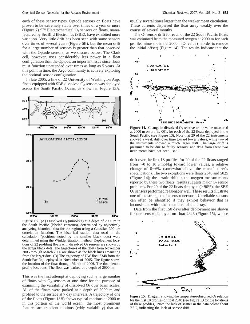
In late 2005, a line of 22 University of Washington Argofloats equipped with SBE dissolved O2 sensors was deployedacross the South Pacific Ocean, as shown in Figure 13A.

This was the first attempt at deploying such a large numberof floats with O2 sensors at one time for the purpose ofexamining the variability of dissolved O2 over basin scales.All of the floats were parked at a depth of 2000 m andprofiled to the surface at 7 day intervals. A trajectory of oneof the floats (Figure 13B) shows typical motions at 2000 min this portion of the world ocean: the most prominentfeatures are transient motions (eddy variability) that are

usually several times larger than the weaker mean circulation.These currents dispersed the float array weakly over thecourse of several months.

The O2 sensor drift for each of the 22 South Pacific floatswas estimated from the measured oxygen at 2000 m for eachprofile, minus the initial 2000 m O2 value (in order to removethe initial offset) (Figure 14). The results indicate that the

drift over the first 18 profiles for 20 of the 22 floats rangedfrom ∼0 to 10 µmol/kg toward lower values, a relativechange of 0-6% (somewhat above the manufacturer’sspecification). The two exceptions were floats 2340 and 5025(Figure 14); the erratic drift in the oxygen measurementsreported by these two floats’ results suggests major O2 sensorproblems. For 20 of the 22 floats deployed (>90%), the SBEO2 sensors performed reasonably well. These results illustrateone of the strengths of a sensor network. Unreliable sensorscan often be identified if they exhibit behavior that isinconsistent with other members of the array.

Data from the first 150 days after deployment are shownfor one sensor deployed on float 2348 (Figure 15), whose

Figure 13. (A) Dissolved O2 (mmol/kg) at a depth of 2000 m inthe South Pacific (labeled contours), determined by objectivelyanalyzing historical data for the region using a Gaussian 300 kmcorrelation function. The historical station data used in thecalculation (positions noted by the smaller black dots) weredetermined using the Winkler titration method. Deployment loca-tions of 22 profiling floats with dissolved O2 sensors are shown bythe larger black dots. The trajectories of the floats from November2005 through March 2006 are shown as the black lines emanatingfrom the larger dots. (B) The trajectory of UW float 2348 from theSouth Pacific, deployed in November of 2005. The figure showsthe location of the float through March of 2006. The dots denoteprofile locations. The float was parked at a depth of 2000 m.

Figure 14. Change in dissolved O2 relative to the value measuredat 2000 m on profile 001, for each of the 22 floats deployed in theSouth Pacific (see Figure 13). Note that 20 of the 22 instrumentsshowed a weak drift over time toward lower values, while two ofthe instruments showed a much larger drift. The large drift ispresumed to be due to faulty sensors, and data from these twoinstruments have not been used.

Figure 15. Diagram showing the temperature-dissolved O2 relationfor the first 18 profiles of float 2348 (see Figure 13 for the locationsof these profiles). Note the lack of scatter in the data below about7 °C, indicating the lack of sensor drift.


trajectory is shown in Figure 13B. The O2 data from profileto profile are quite consistent, forming a tight temperature-O2 relation. At temperatures in excess of about 7°C, thereis some profile-to-profile variability, indicative of seasonalvariations over the 150 day observation period. At temper-atures below about 5°C, where there is little seasonal changein oxygen concentration, there is very little profile-to-profilechange in the temperature-O2 relation (no more than about2 µmol/kg).

The South Pacific at these latitudes has previously beenonly sparsely explored. A comparison between the historicaldatabase and the float-derived O2 estimates is not possiblefor the upper ocean. The seasonal cycle in the upper oceanis too strong, and the variability in the historical O2 databaseis too large for meaningful comparisons to be made. Sincedissolved oxygen has no seasonal cycle at the parking depthof the floats, however, it is possible to compare the floatmeasurements of O2 at 2000 m with the historical data(Figure 13A). The first measured O2 value at 2000 m fromeach of the floats has been compared in Figure 16 to the

value derived from the 2000 m O2 climatology, based onshipboard measurements, at the float position (Figure 13A).The float-derived O2 values at 2000 m are generally lowerthan the climatology, as was also the case with the HOTcomparisons (Figure 6).

There are several possible explanations for these offsets.First, the O2 climatology shown in Figure 13A could beincorrect, due to either faulty historical data, mapping errors,or real changes in the deep O2 distribution in the SouthPacific in recent decades. Each of these potential causesseems unlikely, since the historical data used here are knownto be of excellent quality and other, more recent shipboardmeasurements in this region show values consistent withclimatology. The contouring scheme shown in Figure 13results from objective analysis of the historical data using a300 km Gaussian correlation function. It is possible that thediscrepancies in Figure 16 reflect a problem with the initialcalibration of the O2 sensors at the factory. This would seemto be unlikely, since each sensor is calibrated in a temper-

ature-controlled bath, where sensor-derived values are com-pared to samples pulled from the bath and then analyzed bythe Winkler method. Alternatively, it is possible that the floatO2 sensors could age after leaving the SBE factory. One ofthe features of the SBE oxygen sensor is that they are alwayspolarized with an internal battery. Since the chemical reactionemployed in the Clark cell is operative in air as well asseawater, continuous sensor degradation is possible, althoughthe sensors are in most cases deployed within a few monthsof being manufactured. Presently, each of these scenarios isbeing investigated in order to assess the cause of the initialO2 offsets seen both at Hawaii and in the South Pacific floatdata.

There is seasonal variability in dissolved O2 along theupper portions of the section (Figure 17) that is substantially

larger than the apparent sensor drift of∼5 µmol kg-1 year-1.Throughout the period of November 2005 through March2006, the western South Pacific had relatively high dissolvedO2 in the upper 200 m of the water column and lower valuesin the eastern South Pacific. Below 200 m, there is evidenceof low-O2 water in the eastern portion of the section. Thissignal intensifies through the austral summer as low-oxygenwater is transported poleward along the continental margin.The first profiles (in early November 2005) were from latespring, and the dissolved O2 in the upper 150 m reachedvery high values, in excess of 260µmol/kg in the upperocean. By mid-January 2006 (1 month into austral summer),

Figure 16. The float-derived O2 concentration at 2000 m fromthe first profile for each of the 22 floats deployed at the locationsshown in Figure 13 is plotted against the 2000 m dissolved O2climatology at the position of the first float profile determined usingthe contours shown in Figure 13. The line shows the least-squaresfit between the float O2 and the climatology.

Figure 17. Sections of dissolved O2 in the upper 400 m acrossthe South Pacific, determined from 20 profiling floats deployed inNovember of 2005. Data from two of the floats (2340 and 5025)have not been used in this calculation due to the extreme driftexhibited by these two sensors. The positions of the floats are shownin Figure 13. The positions of the float profiles along the sectionsare noted by the dotted lines.


as the water warmed, O2 was less soluble in near surfacewaters. The surface O2 values decreased by 20-30 µmol/kg. Two months later, in mid-March 2006 (near the end ofaustral summer), the surface O2 had decreased by anadditional 20µmol/kg over much of the South Pacific. It isanticipated that these instruments should continue to operatefor 3-4 more years and, as long as they do not disperse farfrom their initial positions, it will be possible to monitor thevariability in dissolved O2 across the South Pacific usingdata from these profiling floats. This will provide unprec-edented views of oxygen cycling on the scale of an oceanbasin. It will also be possible to assess the performance limitsthat will characterize relatively large chemical sensor arrays.

3.3. The RiverNet System: Monitoring NitrateFlux in Rivers

Human induced changes in the nitrogen cycle on land19,92,93

are recorded in the nitrogen flux of rivers, which integratethe landscape processes in their drainage basins. The globalcreation of fixed nitrogen (Nr) from human activities (mostlyfrom food and energy production) was∼15 Tg N year-1 in1890 and∼140 Tg N year-1 in 1990.94 Increased rates ofanthropogenic Nr production have caused a 4-5-foldincrease in the fixed nitrogen flux in the Mississippi Riverbasin and a 8-13-fold increase in the heavily populatedregions of the Northeast United States and Northern Europe.Assuming that the per capita Nr production rate stays thesame in each region of the world and that the worldpopulation goes to 8.9 billion in 2050,∼190 Tg N year-1

of Nr will be created from human activities globally in 2050.However, if the Nr creation rates of North America (100 kgN capita-1 year-1) are used for the global population of 2050,the Nr created globally in 2050 jumps to 960 Tg N yr-1,which is 7 times greater than the observed 1990 rate and 64times greater than the pre-Haber-Bosch world of 1890. Theseprojections emphasize the need to better understand Nr fluxfrom watersheds.

Most river monitoring programs rely on monthly or weeklysamples,95 which undersample many water quality variations.For example, intensive 2 h sampling over a 102 day periodin the River Main, Northern Ireland, showed that theconcentrations of soluble and particulate P and nitrate N weresignificantly related to short-term variations in flow.96 Usinglog-load, log-flow relationships, the load errors for weeklysampling of the River Main, relative to the high-frequencysamples, ranged from-20% to +45% for fixed N and Ploads.96 These results suggest that monitoring at weekly ormonthly intervals, which creates a bias toward low-flowconditions, can produce large errors when estimating rivernutrient loads. However, more intensive river samplingprograms cannot be easily sustained and in situ monitoringsystems that make measurements in the water and transmitdata daily or in real time are required.86

The RiverNet program was created in 1999 to continuouslymonitor water quality and nitrate flux in the Neuse Riverbasin of North Carolina on the Atlantic Coastal plain. Nitrateconcentrations and discharge measurements have been madefor 5 years at eight different stations (http://rivernet.ncsu.edu).During the 2001-2004 period, nitrate concentration mea-surements were made hourly with WS Envirotech NAS 2Enitrate analyzers.17 The NAS 2E requires chemicals andstandards that are prepared and maintained with steriletechniques to avoid loss of nitrate in standards. The NAS2E can make∼720 unattended measurements with one

chemical payload, so it must be serviced every three weeksfor hourly interval measurements. Stage measurements weremade every 15 min by a USGS gauge station or a YSI 9620Sonde, and converted to discharge with standard rating curvetechniques. Nitrate concentrations were interpolated to 15min intervals and combined with the discharge measurementsto estimate flux. In 2004, Satlantic ISUS UV nitrate analyzerssimilar to those described by Johnson and Coletti8 weredeployed in the basin and used to make measurementssynchronously with the stage measurements at 15 minintervals. The UV nitrate analyzers are sensitive to sedimentaccumulations on the optics during high-flow turbidityevents. This problem was addressed by cleaning the opticswith an automated, high-pressure water pump before UVmeasurements were made.

Five-year records of nitrate concentration and river floware shown at a station below a large wastewater treatmentplant in the upper Basin (Figure 18A) and in the lower basinjust above the tidal influence of the Neuse River estuary(Figure 18B). Large variations in nitrate concentrations wereobserved throughout the 5 year records at each station inthe Basin at all frequencies that were sampled. Theseconcentration variations are found during high- and low-flow conditions and may bias flux estimates. To illustratethe potential bias of undersampling the high-frequency nitrateconcentration variations, daily grab sample results werecompared to NAS-2E measurements at hourly intervals andISUS nitrate concentration measurements at 15 min intervalsover a 4 day period at a station in the upper river basin(Figure 19). A 0.45 mg/L concentration spike is seen in thehighest frequency data. The daily sample interval resolvedonly a 0.1 mg/L concentration change over this same period,while the hourly sample interval resolved a 0.25 mg/Lconcentration peak or only∼55% of the peak height.

Long-term monthly and weekly monitoring records ofnutrient concentrations in the upper portion of the NeuseRiver Estuary (NRE) suggest that phosphorus concentrationshave decreased since the 1988 basin-wide ban on phosphatein detergents but that nitrate concentrations have notsignificantly changed over the same period of time or mayhave been slowly rising since 1996.97 Nitrate flux anddischarge at the RiverNet station immediately above the NREfor the 2001-2006 period show large interannual andmonthly flux variability (Figure 18C). The year 2003 was aperiod of high discharge and high nitrate flux, while 2001-2002 was a period of drought. Monthly nitrate flux averageshave annual decreasing trends where fluxes are high in thewinter and spring and then decrease during the summer andfall. The longer term 5 year trend in the Neuse River showsa slight increase in N flux, similar to the trends observed inthe estuary. However, the long-term flux trends bear littlesimilarity to the concentration trends, which suggests thatnutrient concentrations alone are not reliable indicators ofnutrient flux, which controls estuarine water quality. Thisriver N flux data emphasizes that long-term high-resolutionrecords are required to capture the large inter annualvariations in these river systems and that average concentra-tions do not necessarily correlate to nutrient flux and changesin water quality.

Improved monitoring technologies with higher temporalresolution are required to eliminate errors in our N fluxestimates from watersheds, particularly in watersheds affectedby waste treatment point sources. The sampling frequencyrequired to reliably estimate river N load will be related to


discharge variations and the relationship between N con-centrations and flow. However, there is much that remainsto be learned about N flux in watersheds. It may be that thenitrogen concentration variations or “noise” seen in high-temporal-resolution concentration records is actually a signalthat can help identify the importance of different N sourceson a watershed scale. Managing surface water quality willbe crucial in the future, as population growth increasessewage discharges into surface waters and as groundwaterresources are overcommitted or contaminated. Accuratesurface water quality monitoring will be essential to make

policy decisions to meet our population’s water resourcesneeds in the future.

3.4. Land/Ocean Biogeochemical ObservatoryThe large nutrient loads carried by rivers are focused into

the coastal ocean through estuaries.6,19 These regions aredifficult to monitor with sufficient temporal resolutionbecause the interactions of river flow, tidal oscillations, andstratified water columns can produce rapid changes inconcentration. An example of an operational estuarineobservatory that is capable of providing the chemicalmeasurements that address the coupling of nutrient inputsand ecosystem response at the appropriate spatial andtemporal scale is the Land/Ocean Biogeochemical Observa-tory (LOBO) located in Elkhorn Slough, CA. The watershedis dominated by row crops, and the climate allows two tothree harvests per year, which leads to high fertilizerapplication rates. The observatory network consists ofmoorings deployed throughout the 11 km waterway thatextends inland from the Monterey Bay coastline (Figure 20).Each mooring is equipped with physical and chemical sensorsand a telemetry system for data transmission via a wireless

Figure 18. A 5 year time series of nitrate concentrations measuredwith in situ sensors (gray line), nitrate measured in discrete samples(diamonds), and river stage (black line) in the upper Neuse RiverBasin just below a wastewater treatment plant (A) and in the lowerNeuse River Basin just above the Neuse River Estuary (B). (C)Five year monthly average nitrate concentrations (solid circles) andnitrate flux (gray bars) in the lower Neuse River Basin immediatelyabove the Neuse River Estuary. The 5 year flux regression trend(solid black line) increases, but there is large monthly N fluxvariability.

Figure 19. Comparison of grab samples (gray circles), hourlymeasurements in situ with a NAS-2E analyzer (open diamonds),and 15 min nitrate measurements with an ISUS optical nitrate sensor(black circles) during a nitrate concentration spike in the upperNeuse River basin.

Figure 20. Map of Elkhorn Slough, CA, showing the location ofthe moorings that house the sensors for the Land/Ocean Bio-geochemical Observatory. Data from each mooring is accessibleat http://www.mbari.org/lobo.


network. Nitrate and oxygen are measured with opticalsensors.8,36 Data from each instrument is collected hourlyby a microprocessor-based mooring controller and transmit-ted by wireless radio to a computer at the Monterey BayAquarium Research Institute in Moss Landing, CA. Oncethe data is received, it is made available through the Internetat http://www.mbari.org/lobo.

The 2.5-year-long data set from the LOBO L01 mooringlocated approximately 1 km inland from Monterey Bay(Figure 20) reveals the relationship between nitrate, salinity,and rainfall in the lower estuary (Figure 21). Nearly all of

the rainfall comes during winter, and each of the three wintersthat have been monitored autonomously with the LOBOnetwork are characterized by periods of high nitrate con-centrations and low salinities. The maximum nitrate con-centrations (>400µM) occur during or after rainfall eventsand can be more than an order of magnitude higher thanthose in typical surface marine waters (0-20 µM). Duringlong periods with little or no rainfall (typically May throughNovember) the nitrate concentrations are much lower thanthe winter values. The high nitrate concentrations and lowsalinities are produced by runoff from the watershed thatflows through cultivated fields and strips fertilizers from thesoil.

Surprisingly, brief periods of low salinity and high nitratecan also persist during summer (Figures 21 and 22). Amechanistic understanding of nitrate inputs was identified

by examining data from across the chemical sensor networkat short time scales. Data from the sensor network recordshigh-nitrate, low-salinity water moving from the mouth ofElkhorn Slough toward the inland regions during the risingtide (Figure 23). High nitrate pulses first appear shortly after

low tide at the L01 mooring near the mouth of the Slough.These pulses appear at the L04 mooring in mid-Slough lateron the tide (Figure 23). They reach the L02 mooring at thehead of the Slough at high tide. The two freshwater pointsource regions of Elkhorn Slough are Carneros Creek at thehead of the waterway and the Old Salinas River near theMouth (Figure 20). The data shown in Figure 23 demon-strates that the high nitrate pulses originate at the Old SalinasRiver in the lower estuary and propagate landward, a resultthat is contrary to intuition. The salinity at the L03 mooring,

Figure 21. Salinity (A) and nitrate (B) at the L01 mooring of theLand/Ocean Biogeochemical sensor network measured from No-vember 2003 to April 2006. Also shown is daily precipitation (C)at a nearby weather station. Nitrate was measured with an opticalnitrate sensor.8

Figure 22. Nitrate-salinity relationship at mooring L03 for theperiods March 2005 (filled circles), August 2005 (open circles),and December 2005 (open triangles).

Figure 23. Nitrate and salinity, over a 4 day period, at threelocations in Elkhorn Slough, CA: (A) L01, 1.0 km inland (fromthe Highway 1 bridge); (B) L04, 4.0 km inland; and (C) L02, 6.9km inland. The solid line indicates the relative tide height.


close to the Old Salinas River, fluctuates between nearly freshand nearly marine water over the daily tidal cycle during allseasons of the year. This results from the tidally driven flowof salty water from Monterey Bay upstream to L03 at hightide and from freshwater from the Old Salinas River thatflows past the mooring toward the ocean during low tide.During the dry season, the freshwater source is irrigationrunoff from the intense agriculture in the Salinas Valley. Inwet periods, the freshwater comes from precipitation thatflows over and through the fields. This produces a high-nitrate, low-salinity source of water at L03 (Figure 22) thatenters the mouth of Elkhorn Slough during low tides. Thishigh-nitrate, low-salinity water is then carried inland by therising tide. The nitrate loading in the source changes on aseasonal basis as the balance between irrigation water andprecipitation changes.

The nutrients carried into Elkhorn Slough are linked toelevated rates of primary production, and this must influencethe daily changes in oxygen concentration.46 However, thediel variation in O2 concentration may also be influencedby variability in physical processes. Long-term observationswith a sensor network are key to the deconvolution of theimportant frequencies that drive spatial and temporal vari-ability of O2. For example, O2 concentrations in the mainchannel exhibit repeatable patterns in diel variability thatfluctuate at the spring-neap tidal period of 14 days (Figure24). These patterns are repeated at each station in the networkand must be produced by an interaction between primaryproduction, respiration, and the tidally driven residence timeof water in the estuary.

4. Conclusions and Future Prospects

In this review, we have summarized the work that is beingdone to develop chemical sensor networks that can be usedfor sustained and autonomous observations within naturalaquatic systems. There is now a set of chemical sensors thatare clearly capable of operating in situ for long periods oftime. These sensors have demonstrated remarkable perfor-mance under very strenuous conditions. They validate thefeasibility of making accurate chemical measurements indifficult environments for long time periods with no humanintervention. While the data returned by these sensors, insome cases, do not match the highest precisions andaccuracies available with laboratory measurements, thecontinuous data records that they return can provide a muchbroader perspective on environmental processes. The situ-ation is, in some regards, similar to measurement of oceanchlorophyll concentrations using satellite-borne ocean colorsensors. The satellite measurements at any one surfacelocation are not nearly as precise or accurate as laboratorybased measurements of chlorophyll.98 However, the globalpicture returned by satellites is much richer and revealsprocesses that could not be detected by shipboard samplecollection. In this same sense, the data that have beenreturned with autonomous chemical sensor systems haveprovided an unprecedented view of biogeochemical cyclingthat could not be obtained with conventional sampling. It isclearly possible to consider the operation of global-scalechemical sensor networks.

The technologies that enable long-term, autonomousobservations will be expanded to additional chemicals. Aparticularly vital need exists for pH or other carbon systemsensors that can complement the existing pCO2 sensors andwhich can be used for profiling to ocean depths. In situsensors also demonstrate the role that chemical speciationplays in determining the bioavailability of ecologicallyimportant chemicals.34 Measurements of chemical speciationhave not yet been made in situ for long time periods, butthere is a critical need to develop this capability. Long-term,in situ measurements of trace elements such as iron are alsocritical for our understanding of the role that they play instructuring aquatic ecosystems. Efforts to develop in situanalyzers that are capable of detecting trace elements atsubnanomolar concentrations, which are typical of the marineenvironment,3 are just beginning.99

Existing sensors can also be adapted to additional plat-forms. For example, it appears to be straightforward tomodify the optical nitrate sensors presently employed inmoored applications for use on profiling floats.8 In combina-tion with oxygen sensors, this would allow observations ofthe processes that drive primary production (nutrient avail-ability) and the ecosystem response (oxygen production andconsumption). However, it is also clear that most chemicalspecies will still have to be analyzed in samples that arereturned to the laboratory. The rate of progress in developingnew sensors capable of long-term operation is not rapidenough to anticipate the time when a much broader suite ofchemicals can be sensed autonomously. One of the significantroles of a long-term chemical sensor network will be toprovide the contextual information on variations in majorbiogeochemical processes within which more focused en-vironmental studies can be made using more complexinstrumentation.

Figure 24. Oxygen at three locations in Elkhorn Slough, CA: (A)L01, 1 km inland (from Monterey Bay); (B) L04, 3 km inland;and (C) L02, 8 km inland. Also shown is the relative change inwater depth (m) driven by the tidal cycle (D).


5. AcknowledgmentsWork at MBARI was supported by the National Science

Foundation through the Biocomplexity in the EnvironmentProgram Grant ECS-0308070 and by a grant from the Davidand Lucile Packard Foundation. Research at the Universityof Washington was supported by National Oceanic andAtmospheric Administration Grant NA17RJ1232 Task 2 andby Office of Naval Research Contract ONR NOOO14-03-1-0446. Research at North Carolina State University wassupported by National Science Foundation Grant GEO-0303195 and by the North Carolina Department of Environ-ment and Natural Resources.

6. References(1) Byrne, R.; Diamond, D.Nat. Mater.2006, 5, 421.(2) Emery, W. J.; Thomson, R. E.Data analysis methods in physical

oceanography, 2nd Ed.; Elsevier: Amsterdam, Holland, 2001; 638pp.

(3) Johnson, K. S.; Coale, K. H.; Jannasch, H. W.Anal. Chem.1992,64, 1065A.

(4) de Jonge, V. N.; Elliott, M.; Brauer, V. S.Mar. Pollut. Bull. 2006,53, 5.

(5) Magnuson, J. J.BioScience1990, 40, 495.(6) National Research Council.Clean coastal waters: understanding and

reducing the effects of nutrient pollution; National Academy Press:Washington, DC, 2000; 405 pp.

(7) Johnson, K. S.; Coletti, L. J.; Chavez, F. P.Deep-Sea Res. I2006,53, 561.

(8) Johnson, K. S.; Coletti, L. J.Deep-Sea Res. I2002, 49, 1291.(9) Bell, J.; Betts, J.; Boyle, E.Deep-Sea Res. I2002, 49, 2103.

(10) Jannasch, H. W.; Wheat, C. G.; Plant, J. N.; Kastner, M.; Stakes, D.S. Limnol. Oceanogr.: Methods2004, 2, 102.

(11) Wallace, D. W. R.; Wirick, C. D.Nature1992, 356, 694.(12) McGillicuddy, D. J., Jr.; Robinson, A. R.; Siegel, D. A.; Jannasch,

H. W.; Johnson, R.; Dickey, T. D.; McNeil, J.; Michaels, A. F.;Knapp, A. H.Nature1998, 394, 263.

(13) McNeil, J. D.; Jannasch, H. W.; Dickey, T.; McGillicuddy, D.;Brzezinski, M.; Sakamoto, C. M.J. Geophys. Res.1999, 104, 15537.

(14) Chavez F. P.; Strutton, P. G.; Friederich, G. E.; Feely, R. A.; Feldman,G. C.; Foley, D. G.; McPhaden, M. J.Science1999, 286, 2126.

(15) Friederich, G. E.; Walz, P. M.; Burczynski, M. G.; Chavez, F. P.Prog. Oceanogr.2002, 54, 185.

(16) Sakamoto, C. M.; Karl, D. M.; Jannasch, H. W.; Bidigare, R. R.;Letelier, R. M.; Walz, P. M.; Ryan, J. P.; Polito, P. S.; Johnson, K.S.J. Geophys. Res.2004, 109, C05032 (doi:10.1029/2003JC001976).

(17) Hydes, D. J.; Wright, P. N.; Rawlinson, M. B. InChemical sensorsin oceanography; Varney, M. S., Ed.; Gordon and Breach: Amster-dam, The Netherlands, 2000; pp 95-105.

(18) Baehr, M. M.; DeGrandpre, M. D.Limnol. Oceanogr.2004, 49, 330.(19) Vitousek, P. M.; Aber, J. D.; Howarth, R. W.; Likens, G. E.; Matson,

P. A.; Schindler, D. W.; Schlesinger, W. H.; Tilman, D. G.Ecol.Appl. 1997, 7, 737.

(20) Rojstaczer, S.; Sterling, S. M.; Moore, N. J.Science2001, 294, 2450.(21) Jackson, R. B.; Carpenter, S. R.; Dahm, C. N.; McKnight, D. M.;

Naiman, R. J.; Postel, S. L.; Running, S. W.Ecol. Appl.2001, 11,1027.

(22) Battle, M.; Bender, M. L.; Tans, P. P.; White, J. W. C.; Ellis, J. T.;Conway, T.; Francey, R. J.Science2000, 287, 2467.

(23) Keeling, R. F.; Shertz, S. R.Nature1992, 358, 723.(24) Roemmich, D.; Riser, S.; Davis, R.; Desaubies, Y.Mar. Technol.

Soc. J.2004, 38, 31.(25) Lewis, E. L.IEEE J. Oceanogr. Eng.1980, 5, 3.(26) Schlitzer, R.EOS Trans. Am. Geophys. Union2000, 81, 45.(27) Kortzinger, A.; Shimanski, J.; Send, U.; Wallace, D.Science2004,

306, 1337.(28) Buffle, J., Horvai, G., Eds.In situ monitoring of aquatic systems;

Chemical analysis and speciation; IUPAC Series on Analytical andPhysical Chemistry of Environmental Systems, Vol. 6; Wiley:Chichester, England, 2000; 623 pp.

(29) Varney, M., Ed.Chemical sensors in oceanography; Gordon andBreach: Amsterdam, The Netherlands, 2000; 333 pp.

(30) Taillefert, M.; Luther, G. W.; Nuzzio, D. B.Electroanalysis2000,12, 401.

(31) Daly, K. L.; Byrne, R. H.; Dickson, A. G.; Gallagher, S. M.; Perry,M. J.; Tivey, M. K. Mar. Technol. Soc. J.2004, 38, 121.

(32) Volpe, A. M.; Esser, B. K.; Bianchini, G. M.J. Anal. At. Spectrom.2001, 16, 801.

(33) Clark, L. C.Trans. Am. Soc. Artif. Intern. Organs1956, 2, 41.(34) Luther, G. W., III; Rozan, T. F.; Taillefert, M.; Nuzzio, D. B.; Di

Meo, C.; Shank, T. M.; Lutz, R. A.; Cary, S. C.Nature2001, 410,813.

(35) Glud, R. N.; Klimant, I.; Holst, G.; Kohls, O.; Meyer, V.; Kuehl,M.; Gundersen, J. K.Deep-Sea Res. I1999, 46, 171.

(36) Tengberg, A.; Hovdenes, J.; Andersson, H. J.; Brocandel, O.; Diaz,R.; Hebert, D.; Arnerich, T.; Huber, C.; Kortzinger, A.; Khripounoff,A.; Rey, F.; Ronning, C.; Schimanski, J.; Sommer, S.; Stangelmayer,A. Limnol. Oceanogr. Methods2006, 4, 7.

(37) Clayson, C. H. InChemical sensors in oceanography; Varney, M.S., Ed.; Gordon and Breach: Amsterdam, The Netherlands, 2000;pp 107-121.

(38) DeGrandpre, M. D.; Baehr, M. M.Anal. Chem.1999, 71, 1152.(39) Ruzicka, J.; Hansen, E. H.Flow Injection Analysis, 2nd ed.; Wiley:

New York, 1985, 498.(40) Blain, S.; Jannasch, H. W.; Johnson, K. S. InChemical sensors in

oceanography; Varney, M. S., Ed.; Gordon and Breach: Amsterdam,The Netherlands, 2000; pp 49-70.

(41) Johnson, K. S.; Elrod, V. A.; Nowicki, J. L.; Coale, K. H.; Zamzow,H. In In situ monitoring of aquatic systems; Chemical analysis andspeciation; Buffle, J., Horvai, G., Eds.; IUPAC Series on Analyticaland Physical Chemistry of Environmental Systems, Vol. 6; Wiley:Chichester, England, 2000; pp 223-252.

(42) Chavez, F. P.; Wright, D.; Herlien, R.; Kelley, M.; Shane, F.; Strutton,P. G.J. Atmos. Ocean. Technol.2000,17, 215.

(43) Manov, D. V.; Chang, G. C.; Dickey, T. D.J. Atmos. Ocean. Technol.2004, 21, 958.

(44) Odum, H. T.Limnol. Oceanogr.1956, 1, 103.(45) Rabalais, N. N.Ambio2002, 31, 102.(46) Caffrey, J. M.EnViron. Monit. Assess.2003, 81, 207.(47) Emerson, S.; Stump, C.; Johnson, B.; Karl, D. M.Deep-Sea Res. I

2002, 49, 941.(48) Beck, N. G.; Fisher, A. T.; Bruland, K. W.Mar. Ecol. Prog. Ser.

2001, 217, 43.(49) Rudnick, D. L.; Davis, R. E.; Eriksen, C. C.; Fratantoni, D. M.; Perry,

M. J. Mar. Technol. Soc. J.2005, 38, 48.(50) Karl, D. M.; Lucas, R.Deep-Sea Res. II1996, 43, 129.(51) Fofonoff, N. P.J. Geophys. Res.1985, 90, 3332.(52) Grasshoff K. InMethods of Seawater Analysis, 2nd ed.; Grasshoff,

K., Ehrhardt, M., Kremling, K., Eds.; Verlag Chemie: New York,1983.

(53) Demas J. N.; DeGraff, B. A.; Coleman, P. B.Anal. Chem.1999, 71,793A.

(54) Kortzinger, A.; Schimanski, J.; Send, U.J. Atmos. Ocean. Technol.2005, 22, 302.

(55) Glazer, B. T.; March, A. G.; Stierhoff, K.; Luther, G. W.Anal. Chim.Acta 2004, 518, 93.

(56) Atkinson, M. J.Limnol. Oceanogr.1988, 33, 141.(57) Berg, P.; Roy, H.; Janssen, F.; Meyer, V.; Jorgensen, B. B.; Huettel,

M.; de Beer, D.Mar. Ecol. Prog. Ser.2003, 261, 75.(58) McNeil, C. L.; Johnson, B. D.; Farmer, D. M.Deep-Sea Res. I1995,

42, 819.(59) Kennett, J. P.; Cannariato, K. G.; Hendy, I. L.; Behl, R. J.Science

2000, 288, 128.(60) Kim, G.; Hwang, D.-W.Geophys. Res. Lett.2002, 29, 1678 (10.1029/

2002GL015093).(61) DeGrandpre, M. D.; Hammar, T. R.; Wallace, D. W. R.; Wirick, C.

D. Limnol. Oceanogr.1997, 42, 21.(62) Hood, E. M.; Merlivat, L.J. Mar. Res.2001, 59, 113.(63) DeGrandpre, M. D.; Hammar, T. R.; Smiith, S. P.; Sayles, F. L.

Limnol. Oceanogr.1995, 40, 969.(64) Lefevre, N.; Ciabrini, J. P.; Michard, G.; Brient, B.; DuChaffaut,

M.; Merlivat, L. Mar. Chem.1993, 42, 189.(65) Friederich, G. E.; Brewer, P. G.; Herlein, R.; Chavez, F. P.Deep-

Sea Res. I1995, 42, 1175.(66) Hanson, P. C.; Bade, D. L.; Carpenter, S. R.; Kratz, T. K.Limnol.

Oceanogr.2003, 48, 1112.(67) Byrne, R. H.; McElligott, S.; Feely, R. A.; Millero, F. J.Deep-Sea

Res. I1999, 46, 1985.(68) Martz, T. R.; Carr, J. J.; French, C. R.; DeGrandpre, M. D.Anal.

Chem.2003, 75, 1844.(69) Watanabe, A.; Kayanne, H.; Nozaki, K.; Kato, K.; Negishi, A.; Kudo,

S.; Kimoto, H.; Tsuda, M.; Dickson, A. G.Mar. Chem.2004, 85,75.

(70) Grasshoff, K., Kremling, K., Erhardt, M., Eds.Methods of SeawaterAnalysis; Wiley: Chichester, England, 1999; 447 pp.

(71) Jannasch, H. W.; Johnson, K. S.; Sakamoto, C. M.Anal. Chem.1994,66, 3352.

(72) Chapin, T. P.; Caffrey, J. M.; Jannasch, H. W.; Coletti, L. J.; Haskins,J. C.; Johnson, K. S.Estuaries2004, 27, 882.

(73) Thouron, D.; Vuillemin, R.; Philippon, X.; Lourenco, A.; Provost,C.; Cruzado, A.; Garcon, V.Anal. Chem.2003, 75, 2601.


(74) Chapin, T. P.; Jannasch, H. W.; Johnson, K. S.Anal. Chim. Acta2002, 463, 265.

(75) Sharples, J.; Moore, C. M.; Abraham, E. R.J. Geophys. Res.2001,106, 14,069.

(76) Sigleo, A.C.; Mordy, C. W.; Stabeno, P.; Frick, W. E.Estuarine,Coastal Shelf Sci.2005, 64, 211.

(77) Weston, K.; Jickells, T. D.; Fernand, L.; Parker, E. R.Estuarine,Coastal Shelf Sci.2004, 59, 559.

(78) Muller, B.; Reinhardt, M.; Gachter, R.J. EnViron. Monit. 2003, 5,808.

(79) Le Goff, T.; Braven, J.; Ebdon, L.; Scholefield, D.J. EnViron. Monit.2003, 5, 353.

(80) Scholefield, D.; Le Goff, T.; Braven, J.; Ebdon, L.; Long, T.; Butler,M. Sci. Total EnViron. 2005, 344,201.

(81) Pressl, A.; Winkler, S.; Gruber, G.Water Sci. Technol.2004, 50,67.

(82) Bishop, J. K. B.; Calvert, S. E.; Soon, M. Y. S.Deep-Sea Res. II1999, 46, 2699.

(83) Bishop, J. K. B.; Davis, R. E.; Sherman, J. T.Science2002, 298,817.

(84) Bishop, J. K. B.; Wood, T. J.; Davis, R. E.; Sherman, J. T.Science2004, 304, 417.

(85) Porter, J.; Arzberger, P.; Braun, H.-W.; Bryant, P.; Gage, S.; Hansen,T.; Hanson, P.; Lin, C.-C.; Lin, F.-P.; Kratz, T.; Michener, W.;Shapiro, S.; Williams, T.Bioscience2005, 55, 561.

(86) Glasgow, H. B.; Burkholder, J. M.; Reed, R. E.; Lewitus, A. J.;Kleinman, J. E.J. Exp. Mar. Biol. Ecol.2004, 300, 409.

(87) Effler, S. W.; O’Donnell, D. M.; Owen, C. J.J. Urban Technol.2002,9, 21.

(88) Vivoni, E. R.; Camilli, R.Comput. Geosci.2003, 29, 457.(89) Wenner, E. L.; Geist, M.Coastal Management2001, 29, 1.(90) Tedesco, M.; Bohlen, W. F.; Howard-Strobel, M. M.; Cohen, D. R.;

Tebeau, P. A.EnViron. Monit. Assess.2003, 81, 35.(91) Grasshoff, K. InMarine Electrochemistry; Whitfield, M., Jagner, D.,

Eds.; John Wiley: Chichester, England, 1981; pp 327-420.(92) Howarth, R. W.Water Sci. Technol.2004, 49, 7.(93) Galloway, J. N.; Dentener, F. J.; Capone, D. G.; Boyer, E. W.;

Howarth, R. W.; Seitzinger, S. P.; Asner, G. P.; Cleveland, C. C.;Green, P. A.; Holland, E. A.; Karl, D. M.; Michaels, A. F.; Porter,J. H.; Townsend, A. R.; Vorosmarty, C. J.Biogeochemistry2004,70, 153.

(94) Galloway, J. N. InTreatise on Geochemistry; Schlesinger, W. H.,Ed.; Biogeochemistry Vol. 8; Elsevier: Oxford, 2005; pp 557-583.

(95) Zhang, Y. K.; Schilling, K.AdV. Water Resour.2005,28, 701.(96) Stevens, R. J.; Smith, R. V.Water Res.1978, 12, 823.(97) Paerl, H. W.; Valdes, L. M.; Joyner, A. R.; Piehler, M. F.; Lebo, M.

E. EnViron. Sci. Technol.2004, 38, 3068.(98) Hooker, S. B.; McClain, C. R.Prog. Oceanogr.2000, 45, 427.(99) Laes, A.; Vuillemin, R.; Leilde, B.; Sarthou, G.; Bournot-Marec, C.;

Blain, S.Mar. Chem.2005, 97, 347.

CR050354E


chemical sensor networks for the aquatic …...chemical sensor networks for the aquatic environment...

Documents