chemistry 155 introduction to instrumental analytical chemistry … lecture 2009 1-294.pdf · chem...
TRANSCRIPT
Chem 155 Unit 1 Page 1 of 316
Page 1 of 316
Chemistry 155 Introduction to Instrumental
Analytical Chemistry Unit 1 Spring 2009 San Jose State University Roger Terrill
Chem 155 Unit 1 Page 2 of 316
Page 2 of 316
1 Overview and Review ........................................................................................ 7 2 Propagation of Error ......................................................................................... 56 3 Introduction to Spectrometric Methods ............................................................ 65 4 Photometric Methods and Spectroscopic Instrumentation ............................... 86 5 Radiation Transducers (Light Detectors): ...................................................... 102 6 Monochromators for Atomic Spectroscopy: ................................................... 116 7 Photometric Issues in Atomic Spectroscopy .................................................. 137 8 Practical aspects of atomic spectroscopy: ..................................................... 151 9 Atomic Emission Spectroscopy ...................................................................... 162 10 Ultraviolet-Visible and Near Infrared Absorption .......................................... 177 11 UV-Visible Spectroscopy of Molecules ........................................................ 195 12 Intro to Fourier Transform Infrared Spectroscopy ........................................ 211 13 Infrared Spectrometry: ................................................................................. 234 14 Infrared Spectrometry - Applications ............................................................ 247 15 Raman Spectroscopy: .................................................................................. 259 16 Mass Spectrometry (MS) overview: ............................................................. 279 17 Chromatography .......................................................................................... 294
Chem 155 Unit 1 Page 3 of 316
Page 3 of 316
1 Overview and Review ........................................................................................ 7
1.1 Tools of Instrumental Analytical Chem. ................................................ 8 1.2 Instrumental vs. Classical Methods. ................................................... 12 1.3 Vocabulary: Basic Instrumental .......................................................... 13 1.4 Vocabulary: Basic Statistics Review .................................................. 14 1.5 Statistics Review ................................................................................ 15 1.6 Calibration Curves and Sensitivity ...................................................... 23 1.7 Vocabulary: Properties of Measurements .......................................... 24 1.8 Detection Limit ................................................................................... 25 1.9 Linear Regression .............................................................................. 31 1.10 Experimental Design: ....................................................................... 35 1.11 Validation – Assurance of Accuracy: ................................................ 43 1.12 Spike Recovery Validates Sample Prep. .......................................... 45 1.13 Reagent Blanks for High Accuracy: .................................................. 46 1.14 Standard additions fix matrix effects:................................................ 47 1.15 Internal Standards ............................................................................ 52
2 Propagation of Error ......................................................................................... 56 3 Introduction to Spectrometric Methods ............................................................ 65
3.1 Electromagnetic Radiation: ................................................................ 66 3.2 Energy Nomogram ............................................................................. 67 3.3 Diffraction ........................................................................................... 68 3.4 Properties of Electromagnetic Radiation: ........................................... 71
4 Photometric Methods and Spectroscopic Instrumentation ............................... 86 4.1 General Photometric Designs for the Quantitation of Chemical Species ................................................................................................................. 87 4.2 Block Diagrams .................................................................................. 88 4.3 Optical Materials ................................................................................ 89 4.4 Optical Sources .................................................................................. 90 4.5 Continuum Sources of Light: .............................................................. 91 4.6 Line Sources of Light: ........................................................................ 92 4.7 Laser Sources of Light: ...................................................................... 93
5 Radiation Transducers (Light Detectors): ...................................................... 102 5.1 Desired Properties of a Detector: ..................................................... 102 5.2 Photoelectric effect photometers ...................................................... 103 5.3 Limitations to photoelectric detectors: .............................................. 105 5.4 Operation of the PMT detector: ........................................................ 106 5.5 PMT Gain Equation: ......................................................................... 107 5.6 Noise in PMT’s and Single Photon Counting: ................................... 109 5.7 Semiconductor-Based Light Detectors: ............................................ 111 5.8 Charge Coupled Device Array Detectors: ........................................ 114
6 Monochromators for Atomic Spectroscopy: ................................................... 116 6.1 Adjustable Wavelength Selectors ..................................................... 117 6.2 Monochromator Designs: ................................................................. 118 6.3 The Grating Equation: ...................................................................... 119 6.4 Dispersion ........................................................................................ 122
Chem 155 Unit 1 Page 4 of 316
Page 4 of 316
6.5 Angular dispersion: .......................................................................... 123 6.6 Effective bandwidth .......................................................................... 125 6.7 Bandwith and Atomic Spectroscopy ................................................. 126 6.8 Factors That Control ΔλEFF ............................................................... 127 6.9 Resolution Defined ........................................................................... 128 6.10 Grating Resolution ......................................................................... 129 6.11 Grating Resolution Exercise: .......................................................... 130 6.12 High Resolution and Echelle Monochromators .............................. 132
7 Photometric Issues in Atomic Spectroscopy .................................................. 137 8 Practical aspects of atomic spectroscopy: ..................................................... 151
8.1 Nebulization (sample introduction): .................................................. 152 8.2 Atomization ...................................................................................... 156 8.3 Flame Chemistry and Matrix Effects ................................................ 157 8.4 Flame as ‘sample holder’: ................................................................ 158 8.5 Optimal observation height: .............................................................. 159 8.6 Flame Chemistry and Interferences: ................................................ 160 8.7 Matrix adjustments in atomic spectroscopy: ..................................... 161
9 Atomic Emission Spectroscopy ...................................................................... 162 9.1 AAS / AES Review: .......................................................................... 163 9.2 Types of AES: .................................................................................. 164 9.3 Inert-Gas Plasma Properties (ICP,DCP) .......................................... 165 9.4 Predominant Species are Ar, Ar+, and electrons .............................. 165 9.5 Inductively Coupled Plasma AES: ICP-AES .................................. 166 9.6 ICP Torches ..................................................................................... 167 9.7 Atomization in Ar-ICP ....................................................................... 168 9.8 Direct Current Plasma AES: DCP-AES ........................................... 169 9.9 Advantages of Emission Methods .................................................... 170 9.10 Accuracy and Precision in AES ...................................................... 172
10 Ultraviolet-Visible and Near Infrared Absorption .......................................... 177 10.1 Overview ........................................................................................ 177 10.2 The Blank ....................................................................................... 178 10.3 Theory of light absorbance ............................................................. 179 10.4 Extinction Cross Section Exercise: ................................................. 180 10.5 Limitations to Beer’s Law: .............................................................. 182 10.6 Noise in Absorbance Calculations: ................................................. 185 10.7 Deviations due to Shifting Equilibria: .............................................. 186 10.8 Monochromator Slit Convolution in UV-Vis: ................................... 189 10.9 UV-Vis Instrumentation: ................................................................. 191 10.10 Single vs. double-beam instruments: ........................................... 192
11 UV-Visible Spectroscopy of Molecules ........................................................ 195 11.1 Spectral Assignments ..................................................................... 196 11.2 Classification of Electronic Transitions ........................................... 197 11.3 Spectral Peak Broadening .............................................................. 198 11.4 Aromatic UV-Visible absorptions: ................................................... 201 11.5 UV-Visible Bands of Aqeuous Transition Metal Ions ...................... 202 11.6 Charge-Transfer Complexes .......................................................... 205
Chem 155 Unit 1 Page 5 of 316
Page 5 of 316
11.7 Lanthanide and Actinide Ions: ........................................................ 206 11.8 Photometric Titration ...................................................................... 207 11.9 Multi-component Analyses: ............................................................ 208
12 Intro to Fourier Transform Infrared Spectroscopy ........................................ 211 12.1 Overview: ....................................................................................... 212
1 molecular vibrations ....................................................................................... 212 12.2 IR Spectroscopy is Difficult! ............................................................ 215 12.3 Monochromators Are Rarely Used in IR ......................................... 216 12.4 Interferometers measure light field vs. time .................................... 217 12.5 The Michelson interferometer: ........................................................ 218 12.6 How is interferometry performed? .................................................. 219 12.7 Signal Fluctuations for a Moving Mirror .......................................... 220 12.8 Mono and polychromatic response ................................................ 222 12.9 Interferograms are not informative: ................................................ 223 12.10 Transforming time frequency domain signals: ......................... 224 12.11 The Centerburst: .......................................................................... 225 12.12 Time vs. frequency domain signals: ............................................. 226 12.13 Advantages of Interferometry. ...................................................... 227 12.14 Resolution in Interferometry ......................................................... 228 12.15 Conclusions and Questions: ......................................................... 232 12.16 Answers: ...................................................................................... 233
13 Infrared Spectrometry: ................................................................................. 234 13.1 Absorbance Bands Seen in the Infrared: ........................................ 235 13.2 IR Selection Rules .......................................................................... 236 13.3 Rotational Activity ........................................................................... 238 13.4 Normal Modes of Vibration: ............................................................ 239 13.5 Group frequencies: a pleasant fiction! ............................................ 242 13.6 Summary: ....................................................................................... 246
14 Infrared Spectrometry - Applications ............................................................ 247 14.1 Strategies used to make IR spectrometry work - ............................ 248 14.2 Solvents for IR spectroscopy: ......................................................... 249 14.3 Handling of neat (pure – no solvent) liquids: .................................. 249 14.4 Handling of solids: pelletizing: ........................................................ 250 14.5 Handling of Solids: mulling: ............................................................ 250 14.6 A general problem with pellets and mulls: ...................................... 251 14.7 Group Frequencies Examples ........................................................ 252 14.8 Fingerprint Examples ..................................................................... 253 14.9 Diffuse Reflectance Methods: ........................................................ 254 14.10 Quantitation of Diffuse Reflectance Spectra: ................................ 255 14.11 Attenuated Total Reflection Spectra: ............................................ 256
15 Raman Spectroscopy: .................................................................................. 259 15.1 What a Raman Spectrum Looks Like ............................................. 261 15.2 Quantum View of Raman Scattering. ............................................. 262 15.3 Classical View of Raman Scattering .............................................. 263 15.4 The classical model of Raman: ...................................................... 265 15.5 The classical model: catastrophe! .................................................. 266
Chem 155 Unit 1 Page 6 of 316
Page 6 of 316
15.6 Raman Activity: .............................................................................. 267 15.7 Some general points regarding Raman: ......................................... 269 15.8 Resonance Raman ........................................................................ 271 15.9 Raman Exercises ........................................................................... 272
16 Mass Spectrometry (MS) overview: ............................................................. 279 16.1 Example: of a GCMS instrument: ................................................... 279 16.2 Block diagram of MS instrument. ................................................... 280 16.3 Information from ion mass .............................................................. 281 16.4 Ionization Sources .......................................................................... 282 16.5 Mass Analyzers: ............................................................................. 287 16.6 Mass Spec Questions: ................................................................... 292
17 Chromatography .......................................................................................... 294 17.1 General Elution Problem / Gradient Elution .................................... 307 17.2 T-gradient example in GC of a complex mixture. ........................... 309 17.3 High Performance Liquid Chromatography .................................... 310 17.4 Types of Liquid Chromatography ................................................... 311 17.5 Normal Phase: ............................................................................... 311 17.6 HPLC System overview: ................................................................. 314 17.7 Example of Reverse-phase HPLC stationary phase: ..................... 315 17.8 Ideal qualities of HPLC stationary phase: ....................................... 316
Chem 155 Unit 1 Page 7 of 316
Page 7 of 316
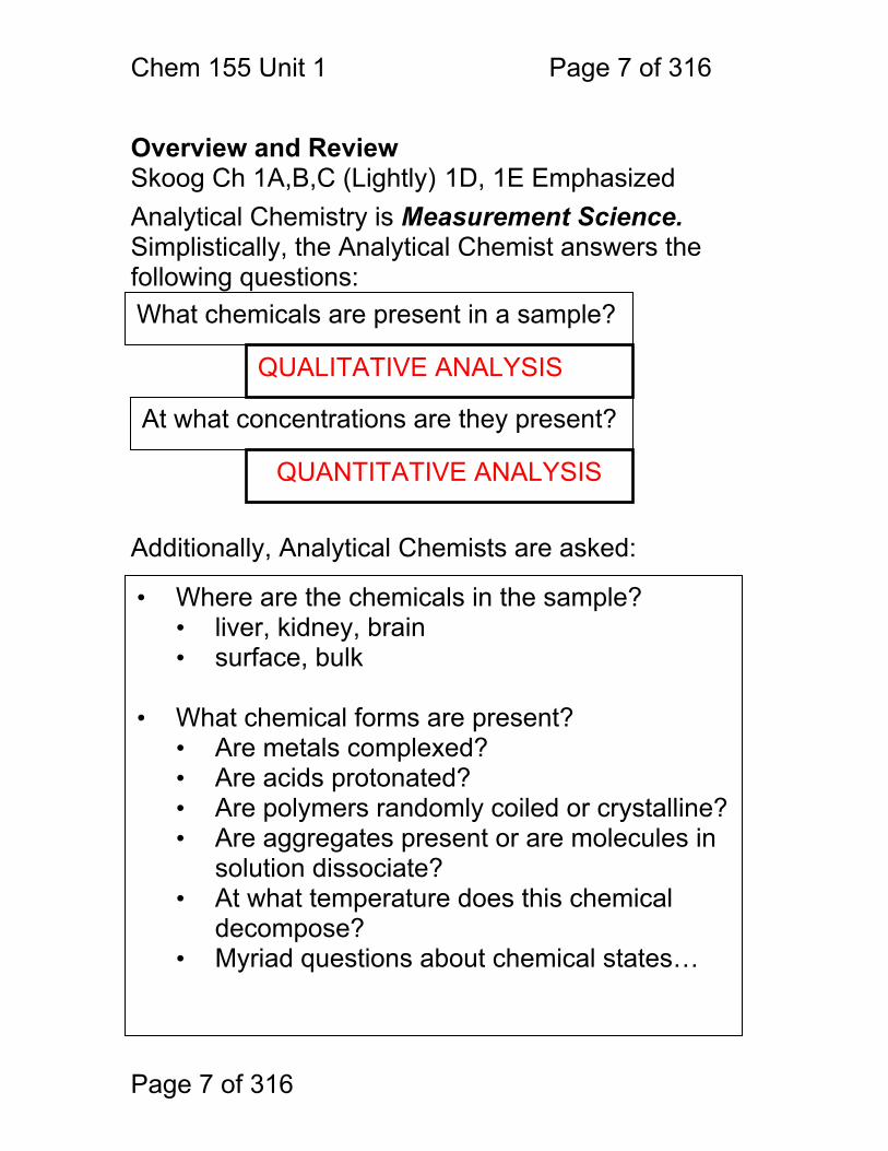
Overview and Review Skoog Ch 1A,B,C (Lightly) 1D, 1E Emphasized Analytical Chemistry is Measurement Science. Simplistically, the Analytical Chemist answers the following questions: Additionally, Analytical Chemists are asked:
What chemicals are present in a sample?
• Where are the chemicals in the sample? • liver, kidney, brain • surface, bulk
• What chemical forms are present?
• Are metals complexed? • Are acids protonated? • Are polymers randomly coiled or crystalline? • Are aggregates present or are molecules in
solution dissociate? • At what temperature does this chemical
decompose? • Myriad questions about chemical states…
QUALITATIVE ANALYSIS
At what concentrations are they present?
QUANTITATIVE ANALYSIS
Chem 155 Unit 1 Page 8 of 316
Page 8 of 316
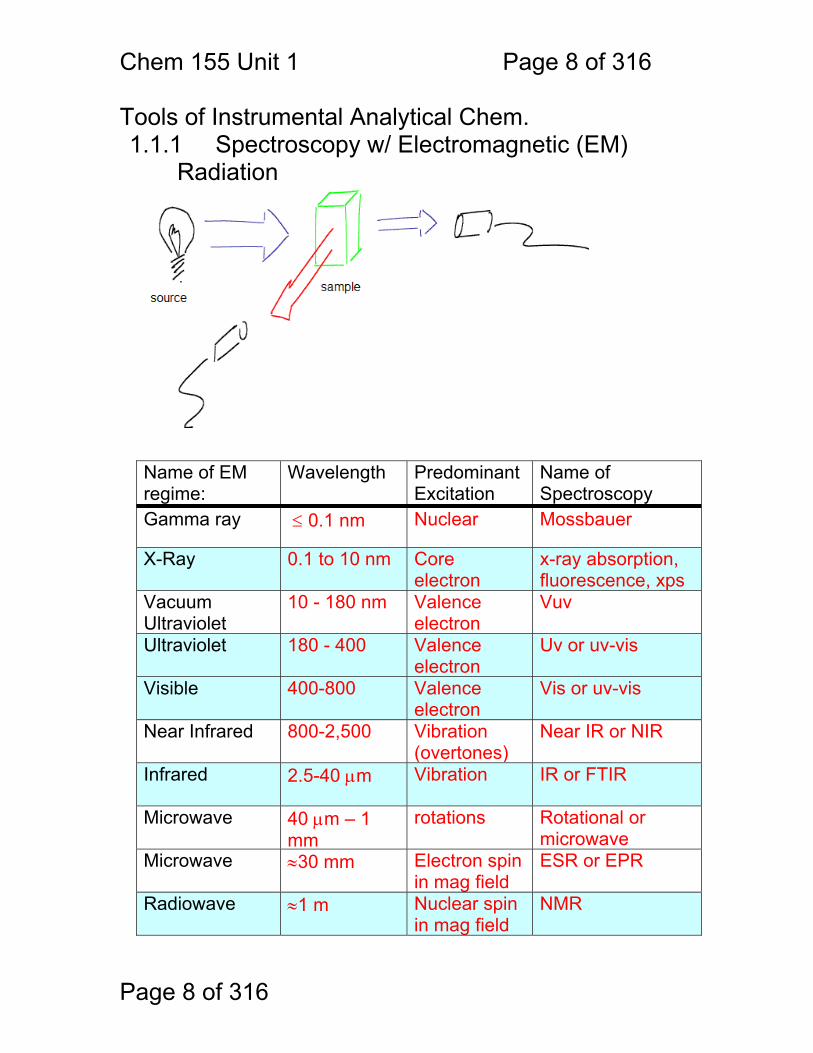
Tools of Instrumental Analytical Chem. 1.1.1 Spectroscopy w/ Electromagnetic (EM)
Radiation Name of EM regime:
Wavelength Predominant Excitation
Name of Spectroscopy
Gamma ray ≤ 0.1 nm Nuclear Mossbauer
X-Ray 0.1 to 10 nm Core electron
x-ray absorption, fluorescence, xps
Vacuum Ultraviolet
10 - 180 nm Valence electron
Vuv
Ultraviolet 180 - 400 Valence electron
Uv or uv-vis
Visible 400-800 Valence electron
Vis or uv-vis
Near Infrared 800-2,500 Vibration (overtones)
Near IR or NIR
Infrared 2.5-40 μm Vibration IR or FTIR
Microwave 40 μm – 1 mm
rotations Rotational or microwave
Microwave ≈30 mm Electron spin in mag field
ESR or EPR
Radiowave ≈1 m Nuclear spin in mag field
NMR
Chem 155 Unit 1 Page 9 of 316
Page 9 of 316
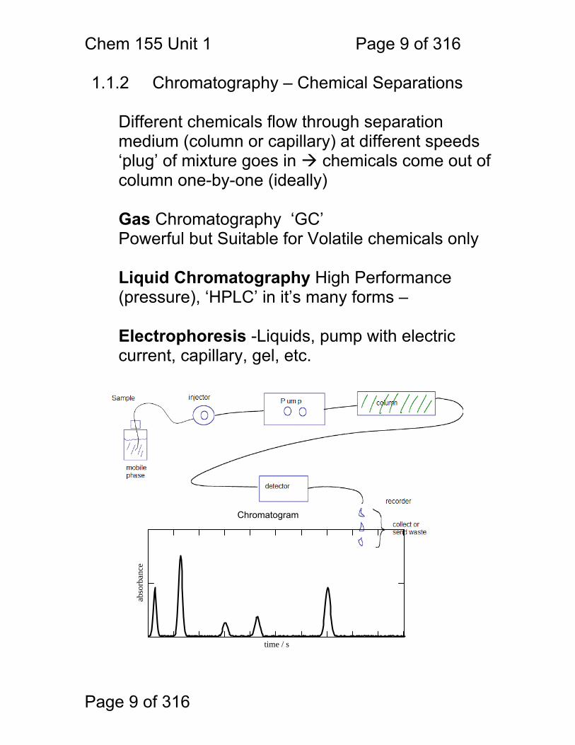
1.1.2 Chromatography – Chemical Separations
Different chemicals flow through separation medium (column or capillary) at different speeds ‘plug’ of mixture goes in chemicals come out of column one-by-one (ideally)
Gas Chromatography ‘GC’ Powerful but Suitable for Volatile chemicals only Liquid Chromatography High Performance (pressure), ‘HPLC’ in it’s many forms – Electrophoresis -Liquids, pump with electric current, capillary, gel, etc.
time / s
abso
rban
ce
Chromatogram
Chem 155 Unit 1 Page 10 of 316
Page 10 of 316
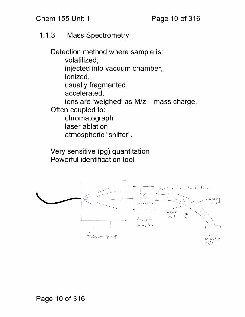
1.1.3 Mass Spectrometry Detection method where sample is: volatilized, injected into vacuum chamber,
ionized, usually fragmented, accelerated, ions are ‘weighed’ as M/z – mass charge.
Often coupled to: chromatograph laser ablation atmospheric “sniffer”.
Very sensitive (pg) quantitation Powerful identification tool
Chem 155 Unit 1 Page 11 of 316
Page 11 of 316
1.1.4 Electrochemistry Simple, sensitive, limited to certain chemicals
Ion selective electrodes (ISE’s): e.g. pH, pCl, pO2 etc. ISE’s measure voltage across a selectively permeable membrane (e.g. glass for pH) E α log[concentration] ISE’s have incredible dynamic range!
pH 4 pH 10 [H+] = 0.0001 0.0000000001 M Dynamic electrochemistry – measure current (i) resulting from redox reactions at an driven by a controlled voltage at an electrode surface
i(E,t) α [concentration] 1.1.5 Gravimetry
Precipitate and weigh products – very precise, very limited
1.1.6 Thermal Analysis Thermogravimetric Analysis TGA Mass loss during heating – loss of waters of
hydration, or decomposition temperature Differential Scanning Calorimetry DSC Heat flow during heating or cooling

Chem 155 Unit 1 Page 12 of 316
Page 12 of 316
Instrumental vs. Classical Methods.
Methods of Analytical Chemistry
Classical
# Chemicals Isolated / hr and amount
(g)
Instrumental
# Chemicals Isolated / hr and amount
(g)
Separation
Extraction 1-2 g High Performance
Liquid Chromatrography
10 ng
Distillation 1-2 g Gas Chromatography 100 ng
Precipitation 1-2 g Electrophoresis 50 pg
Crystallization 1-2 g
Estimated Number of uniquely identifiable molecules by method
Qualitative Speciation
Combination of Color / Smell Melt / Boiling
Point, Solubility Wetting Density
Hardness
100’s
UV-Vis 1,000’s
Infrared 100,000’s
Mass Spectrometry > 106
NMR Spectroscopy > 106
Best Quantitative Precision and Sensitivity
Quantitation Precision
Titration
0.1% 1 ppm
Optical Spectroscopy
0.1% 10-23 M
Gravimetry
0.01% 1 ppm
Mass Spectrometry
0.1% amount 10-13 M 10-4% mass
Colorimetry 10% 1 ppm NMR
Spectroscopy
1% 100
pppm
What are the more precise measurements that you have made and what were they?
Relax, you don’t need to memorize this table – just humor Dr. Terrill while he talks about it.
Chem 155 Unit 1 Page 13 of 316
Page 13 of 316
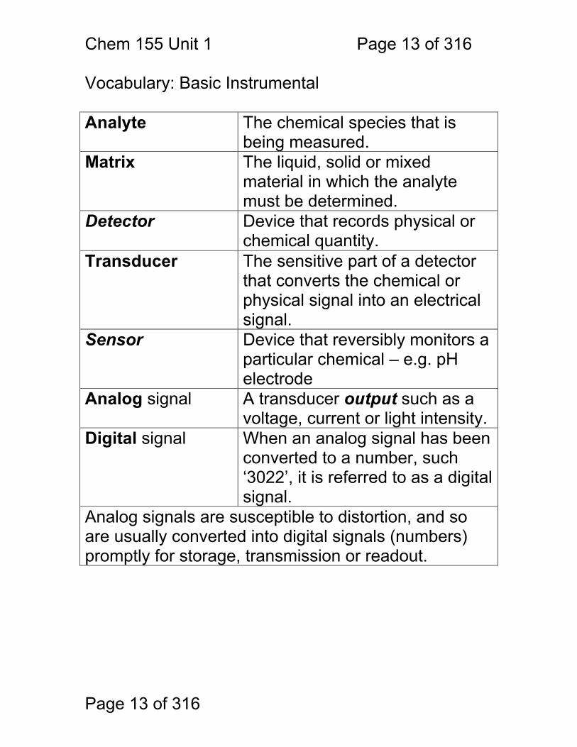
Vocabulary: Basic Instrumental Analyte The chemical species that is
being measured. Matrix The liquid, solid or mixed
material in which the analyte must be determined.
Detector Device that records physical or chemical quantity.
Transducer The sensitive part of a detector that converts the chemical or physical signal into an electrical signal.
Sensor Device that reversibly monitors a particular chemical – e.g. pH electrode
Analog signal A transducer output such as a voltage, current or light intensity.
Digital signal
When an analog signal has been converted to a number, such ‘3022’, it is referred to as a digital signal.
Analog signals are susceptible to distortion, and so are usually converted into digital signals (numbers) promptly for storage, transmission or readout.

Chem 155 Unit 1 Page 14 of 316
Page 14 of 316
Vocabulary: Basic Statistics Review Precision If repeated measurements of the same thing are
all very close to one another, then a measurement is precise. Note that precise measurements may not be accurate (see below).
Random Error Random error is a measure of precision. Random differences between sequential measurements reflect the random error.
Accuracy If a measurement of something is correct, i.e. close to the true value, then that measurement is accurate.
Systematic Error (bias)
Systematic error is the difference between the mean of a population of measurements and the true value.
Histogram A graph of the number or frequency of occurences of a certain measurement versus the measurement value.
Probability Distribution
A theoretical curve of the probability of a certain measured value occurring versus the measured value.
A histogram of a set of data will often look like a Gaussian probability distribution.
Average The sum of the measured values divided by the number of measurements.
.
Median Half of the measurements fall above the median value, and half fall below.
Variance (σ2) A measurement of precision. The sum of the squares of the random measurement errors.
Standard Deviation (σ)
A widely accepted ‘standard’ measurement of precision. The square root of the variance.
Relative Standard Deviation
The standard deviation divided by the mean, and often expressed as : %RSD=σ/xMEAN100%.
Propagaion of Error
When the mean of a set of measurement (x) has a random error (σx), it is reported as x±σx. If we wish to report the result of a calculation y=f(x) based on x, we propagate the error through the calculation using a mathematical method.
xMEANn
xn
n
σ2 n
xMEAN xn2
n 1
σn
xMEAN xn2
n 1
Chem 155 Unit 1 Page 15 of 316
Page 15 of 316
PopulationStandardDeviation: σx
∞N
N
xN μ−( )2∑N
lim→Mean : μ
∞N N
xN∑lim→
N
SampleStandardDeviation:xavg
N
xN∑N
sxN
xN xavg−( )2∑N 1−Average:
Bias or absolute systematic error = xavg μ−
Relative standard deviation = sxavg
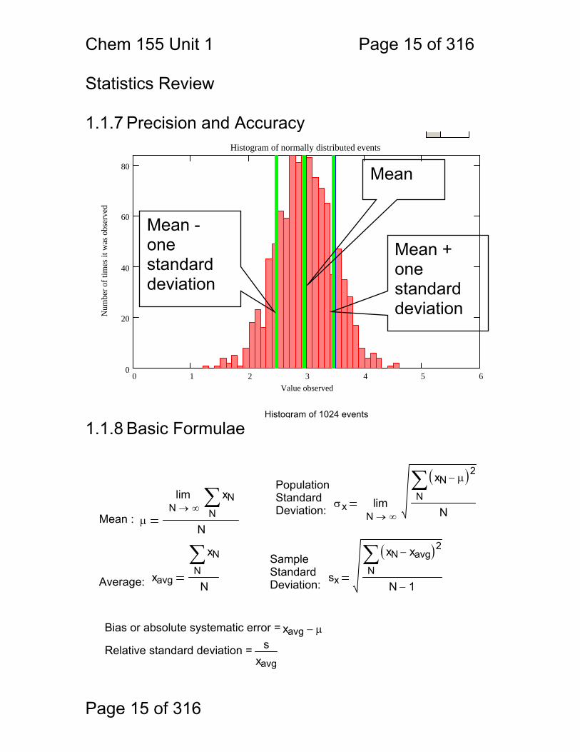
Statistics Review 1.1.7 Precision and Accuracy
0 1 2 3 4 5 60
20
40
60
80
Histogram of normally distributed events
Value observed
Num
ber o
f tim
es it
was
obs
erve
d
Histogram of 1024 events 1.1.8 Basic Formulae
Mean
Mean + one standard deviation
Mean - one standard deviation
Chem 155 Unit 1 Page 16 of 316
Page 16 of 316
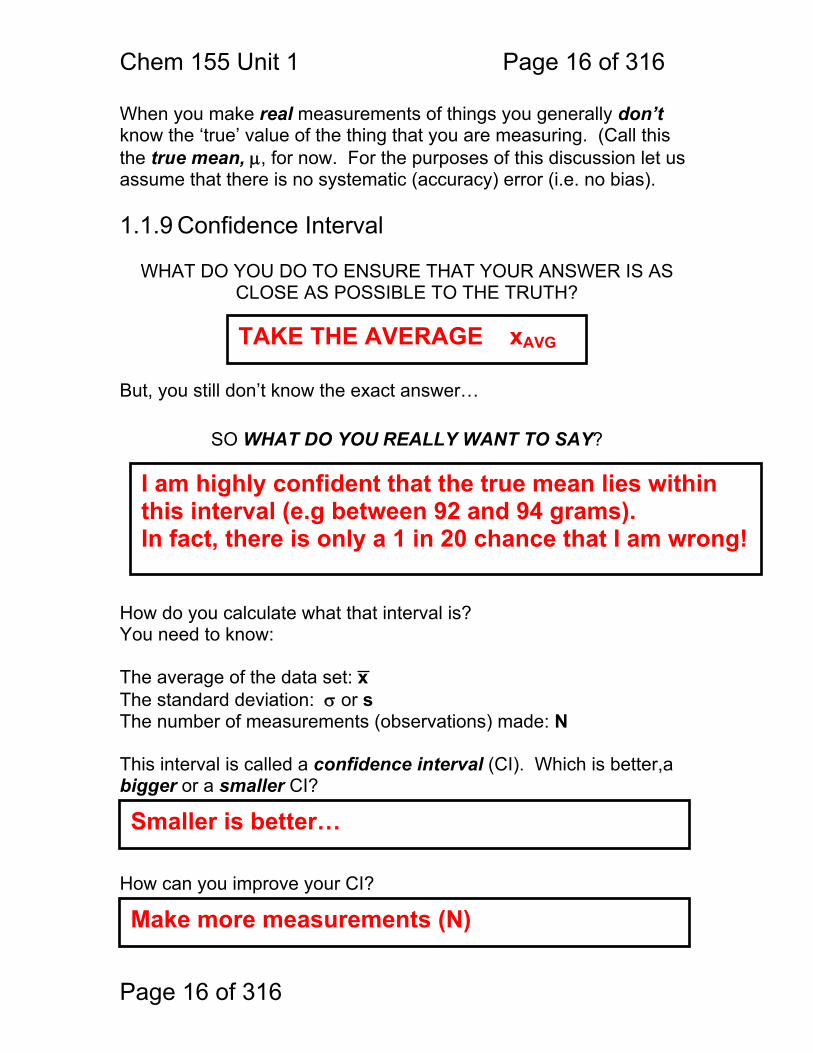
When you make real measurements of things you generally don’t know the ‘true’ value of the thing that you are measuring. (Call this the true mean, μ, for now. For the purposes of this discussion let us assume that there is no systematic (accuracy) error (i.e. no bias). 1.1.9 Confidence Interval
WHAT DO YOU DO TO ENSURE THAT YOUR ANSWER IS AS CLOSE AS POSSIBLE TO THE TRUTH?
But, you still don’t know the exact answer…
SO WHAT DO YOU REALLY WANT TO SAY?
How do you calculate what that interval is? You need to know: The average of the data set: x The standard deviation: σ or s The number of measurements (observations) made: N This interval is called a confidence interval (CI). Which is better,a bigger or a smaller CI? How can you improve your CI?
TAKE THE AVERAGE xAVG
I am highly confident that the true mean lies within this interval (e.g between 92 and 94 grams). In fact, there is only a 1 in 20 chance that I am wrong!
Smaller is better…
Make more measurements (N)
Chem 155 Unit 1 Page 17 of 316
Page 17 of 316
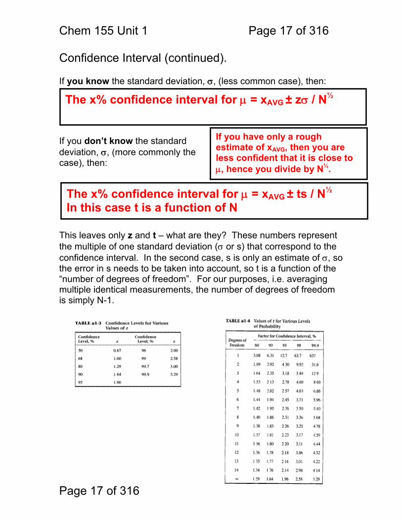
Confidence Interval (continued). If you know the standard deviation, σ, (less common case), then:
If you don’t know the standard deviation, σ, (more commonly the case), then:
This leaves only z and t – what are they? These numbers represent the multiple of one standard deviation (σ or s) that correspond to the confidence interval. In the second case, s is only an estimate of σ, so the error in s needs to be taken into account, so t is a function of the “number of degrees of freedom”. For our purposes, i.e. averaging multiple identical measurements, the number of degrees of freedom is simply N-1.
The x% confidence interval for μ = xAVG ± zσ / N½
The x% confidence interval for μ = xAVG ± ts / N½ In this case t is a function of N
If you have only a rough estimate of xAVG, then you are less confident that it is close to μ, hence you divide by N½.

Chem 155 Unit 1 Page 18 of 316
Page 18 of 316
An example: Assume that we do our best to measure the concentration of basic amines in a fish tank. Our answers are 4.2, 4.6, 4.0. N = XAVG = s = Number of degrees of freedom for confidence interval = 95% confidence limits for μ =
5.0
3.5
5.4
(4.2+4.6+4.0) / 3 = 4.27
(4.2-4.27)2+(4.6-4.27)2+(4.0-4.27)2 3-1
4.27± (4.3*0.31) / (31/2) = 4.27±0.93 or = 4.3 ± 0.9 or = 3 4 to 5 2
4.5
3
3-1=2
= 0.31
Chem 155 Unit 1 Page 19 of 316
Page 19 of 316
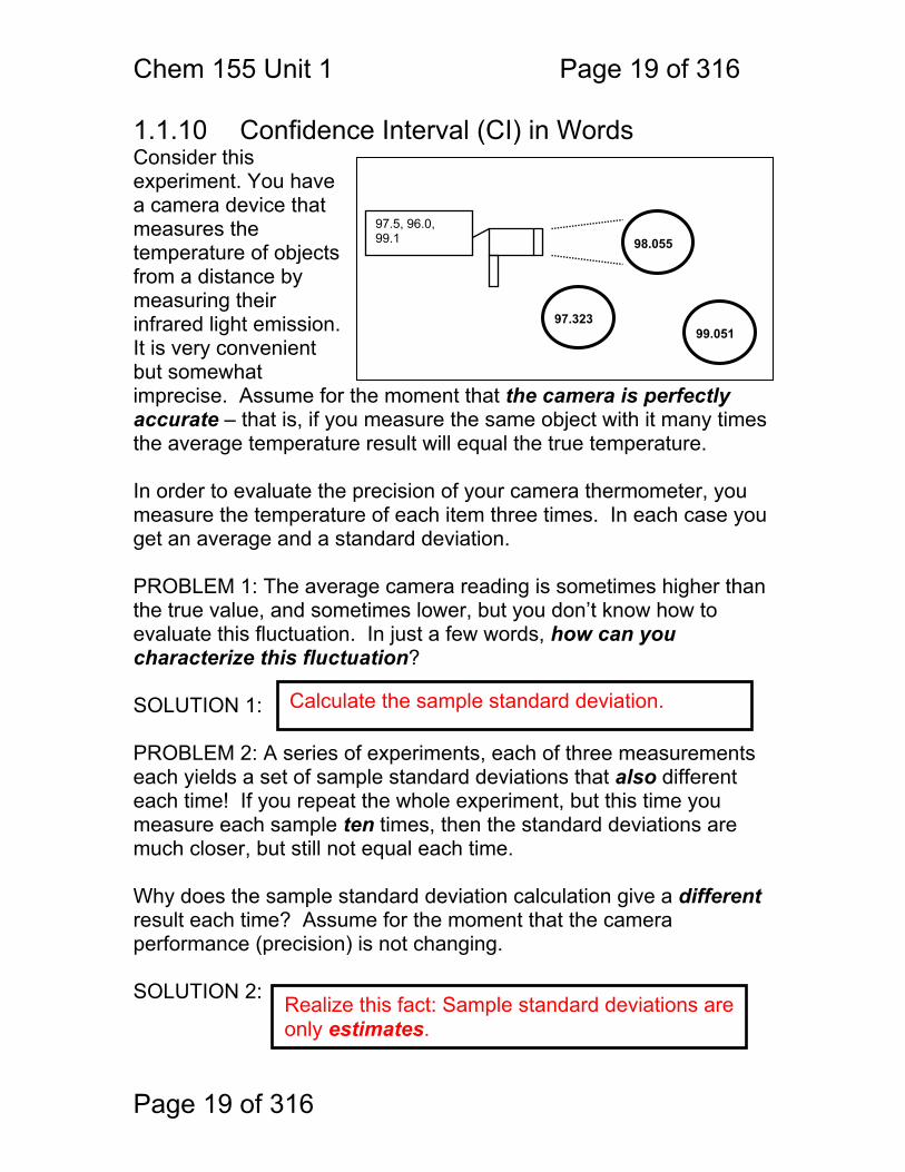
1.1.10 Confidence Interval (CI) in Words Consider this experiment. You have a camera device that measures the temperature of objects from a distance by measuring their infrared light emission. It is very convenient but somewhat imprecise. Assume for the moment that the camera is perfectly accurate – that is, if you measure the same object with it many times the average temperature result will equal the true temperature. In order to evaluate the precision of your camera thermometer, you measure the temperature of each item three times. In each case you get an average and a standard deviation. PROBLEM 1: The average camera reading is sometimes higher than the true value, and sometimes lower, but you don’t know how to evaluate this fluctuation. In just a few words, how can you characterize this fluctuation? SOLUTION 1: PROBLEM 2: A series of experiments, each of three measurements each yields a set of sample standard deviations that also different each time! If you repeat the whole experiment, but this time you measure each sample ten times, then the standard deviations are much closer, but still not equal each time. Why does the sample standard deviation calculation give a different result each time? Assume for the moment that the camera performance (precision) is not changing. SOLUTION 2:
97.5, 96.0, 99.1 98.055
97.323 99.051
Calculate the sample standard deviation.
Realize this fact: Sample standard deviations are only estimates.

Chem 155 Unit 1 Page 20 of 316
Page 20 of 316
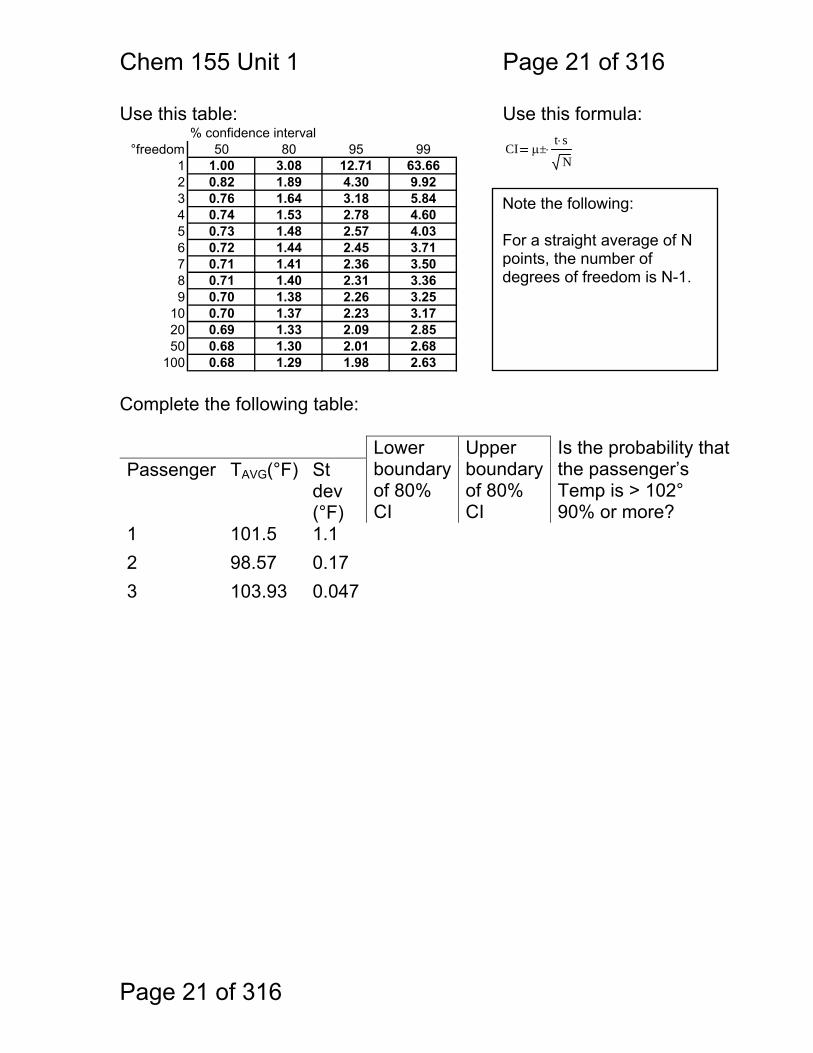
1.1.11 CI PROBLEM: This imperfect camera thermometer is going to be used to screen passengers boarding an airliner. Passengers with a high temperature may have avian flu. Our criterion is this: if there is more than a 90% probability that a given passenger’s temperature exceeds 102°, then we will take him aside and test him for bird flu. We have only moments to acquire three measurements per passenger, so precision is low. Also, the precision is not the same each time. For three passengers we get the following results: Passenger 1: 100.3°, 101.1°, 103.0°. Passenger 2: 98.8°, 98.5°, 98.4° Passenger 3: 104.0°, 103.9°, 103.9° How do we answer the question: does this person’s temperature exceed our 90% / 102° criterion? To answer this, we must accept the following: Assuming that measurements are unbiased (accurate) we can state, for the 80% CI, that there is a 10% probability that the true mean lies below the lower limit of the CI, an 80% probability that the true mean lies within this CI, and a 10% probability that the true mean lies above this CI. So, there is a 90% probability that the true mean lies within or above the 80% CI. For example, if we took some measurements and then computed the 80% CI to be 101.8° to 102.6° then we could say that the probability that the true temperature is 101.4° or higher is 90%.
10% chance
μ is 101.8° or lower
101° 102° 103°
80% chance
101.8° < μ < 102.6°
10% chance
μ is 102.6° or higher
Chem 155 Unit 1 Page 21 of 316
Page 21 of 316
Use this table: Use this formula: % confidence interval
°freedom 50 80 95 991 1.00 3.08 12.71 63.662 0.82 1.89 4.30 9.923 0.76 1.64 3.18 5.844 0.74 1.53 2.78 4.605 0.73 1.48 2.57 4.036 0.72 1.44 2.45 3.717 0.71 1.41 2.36 3.508 0.71 1.40 2.31 3.369 0.70 1.38 2.26 3.25
10 0.70 1.37 2.23 3.1720 0.69 1.33 2.09 2.8550 0.68 1.30 2.01 2.68
100 0.68 1.29 1.98 2.63 Complete the following table: Lower
boundaryof 80% CI
Upper boundary of 80% CI
Is the probability that the passenger’s Temp is > 102° 90% or more?
Passenger TAVG(°F) St dev (°F)
1 101.5 1.1 2 98.57 0.17 3 103.93 0.047
CI μ±t s⋅
N⋅
Note the following: For a straight average of N points, the number of degrees of freedom is N-1.
Chem 155 Unit 1 Page 22 of 316
Page 22 of 316
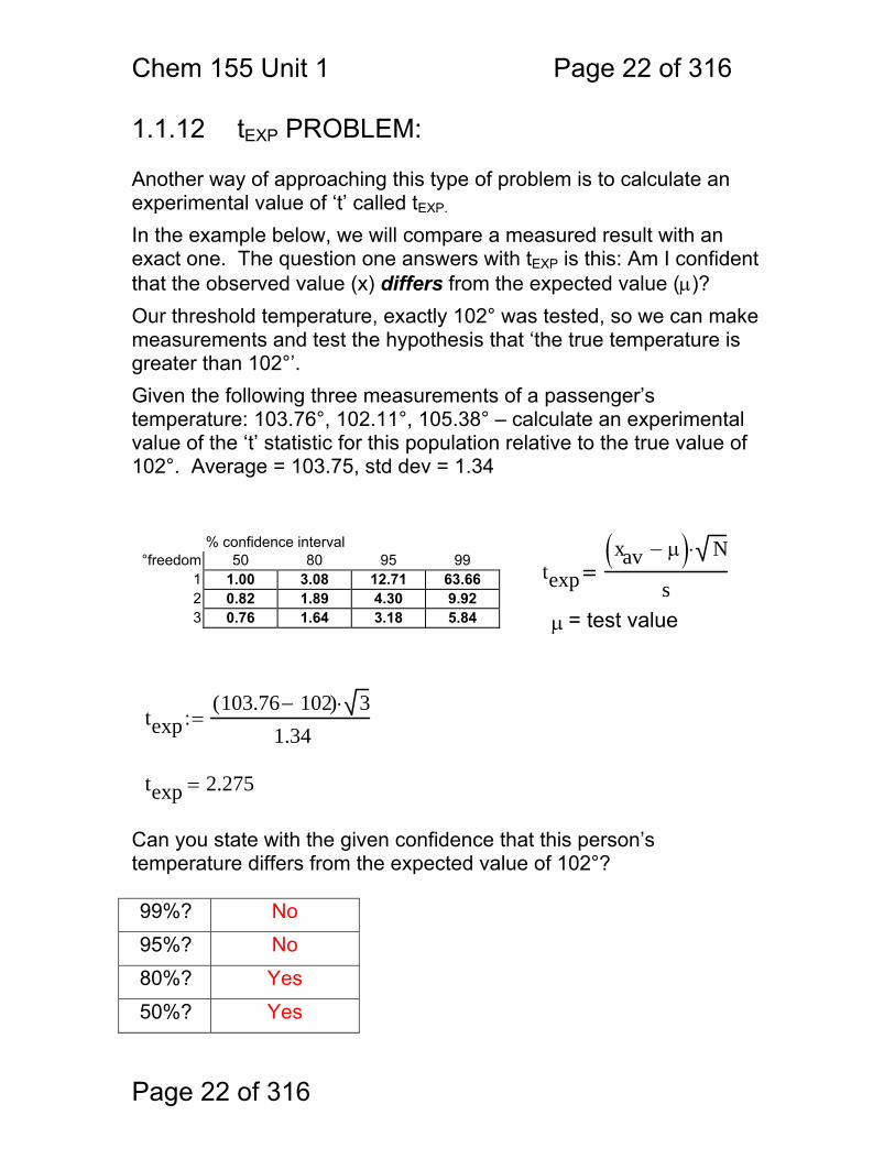
1.1.12 tEXP PROBLEM: Another way of approaching this type of problem is to calculate an experimental value of ‘t’ called tEXP. In the example below, we will compare a measured result with an exact one. The question one answers with tEXP is this: Am I confident that the observed value (x) differs from the expected value (μ)? Our threshold temperature, exactly 102° was tested, so we can make measurements and test the hypothesis that ‘the true temperature is greater than 102°’. Given the following three measurements of a passenger’s temperature: 103.76°, 102.11°, 105.38° – calculate an experimental value of the ‘t’ statistic for this population relative to the true value of 102°. Average = 103.75, std dev = 1.34
% confidence interval °freedom 50 80 95 99
1 1.00 3.08 12.71 63.66 2 0.82 1.89 4.30 9.92 3 0.76 1.64 3.18 5.84
texp103.76 102−( ) 3⋅
1.34:=
texp 2.275= Can you state with the given confidence that this person’s temperature differs from the expected value of 102°? 99%? No 95%? No 80%? Yes 50%? Yes
texpxav μ−( ) N⋅
sμ = test value
Chem 155 Unit 1 Page 23 of 316
Page 23 of 316
ΔS
ΔC= m
0 20 40 60 80 1000
5
10
15
Analyte Concentration (C)
Inst
rum
ent S
igna
l (S)
13.166
0
Si
1000 Ci
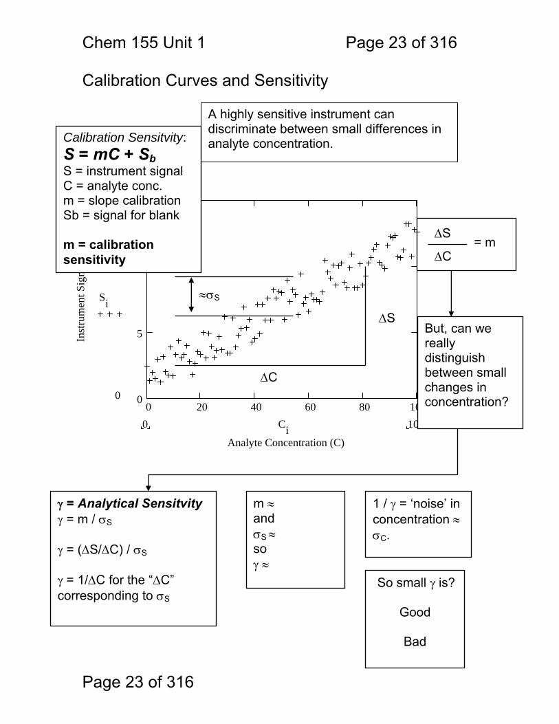
Calibration Curves and Sensitivity
A highly sensitive instrument can discriminate between small differences in analyte concentration.
ΔS
ΔC
≈σS
But, can we really distinguish between small changes in concentration?
Calibration Sensitvity: S = mC + Sb S = instrument signal C = analyte conc. m = slope calibration Sb = signal for blank m = calibration sensitivity
γ = Analytical Sensitvity γ = m / σS γ = (ΔS/ΔC) / σS γ = 1/ΔC for the “ΔC” corresponding to σS
m ≈ and σS ≈ so γ ≈
1 / γ = ‘noise’ in concentration ≈ σC.
So small γ is?
Good
Bad

Chem 155 Unit 1 Page 24 of 316
Page 24 of 316
Vocabulary: Properties of Measurements Sensitivity A detector or instrument that responds to only a
small change in analyte concentration is sensitive. Numerically, the sensitivity of an instrument is the slope of the calibration curve in untis of: signal / unit concentration – often given as ‘m’. Sometimes the detection limit (see below) is called the instrument sensitivity – but this is not correct.
Selectivity The ratio of the sensitivity of an instrument to an analyte to that of an interferant.
Specimen The material removed for analysis – e.g. a given tablet from an assembly line.
Sample The mixture that contains the chemical to be measured – e.g. the blood sample that we want to measure iron in.
Analyte The chemical that is being measured – e.g. the iron in the blood sample.
Calibration Curve A linear or non-linear function relating instrument response (signal) to analyte concentration.
Interferant Another chemical in the sample that either affects the instrument’s sensitivity to the sample or gives a signal of it’s own that may be indistinguishable from the analyte signal.
Detection Limit CMIN or CM
The minimum detectable concentration of analyte. Usually defined as that concentration that gives a signal of magnitude equal to three times the standard deviation in the blank signal.
Limit of Quantitation (LOQ)
The minimum concentration of analyte for which an accurate determination of concentration can be made. The LOQ is typically that concentration for which the signal is 10x the standard deviation of the blank signal.
Limit of Linearity (LOL) The largest concentration for which a calibration curve remains linear.
Linear Dynamic Range (LDR)
The range of concentrations (or signal strengths) between the LOQ and the LOL. An instrument is most useful within its’ LDR.
Chem 155 Unit 1 Page 25 of 316
Page 25 of 316
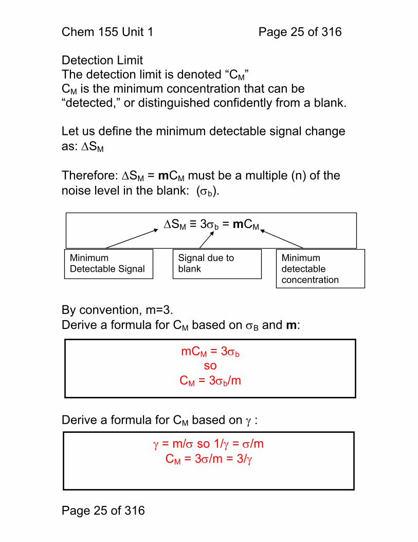
Detection Limit The detection limit is denoted “CM” CM is the minimum concentration that can be “detected,” or distinguished confidently from a blank. Let us define the minimum detectable signal change as: ΔSM Therefore: ΔSM = mCM must be a multiple (n) of the noise level in the blank: (σb).
By convention, m=3. Derive a formula for CM based on σB and m:
Derive a formula for CM based on γ :
γ = m/σ so 1/γ = σ/m CM = 3σ/m = 3/γ
ΔSM ≡ 3σb = mCM
Minimum Detectable Signal
Signal due to blank
mCM = 3σb so
CM = 3σb/m
Minimum detectable concentration

Chem 155 Unit 1 Page 26 of 316
Page 26 of 316
1.1.13 A Graphical Look at Detection Limit (CMIN)
Consider the minimum detectable signal in the context of the confidence interval: SMIN = 3σb + Sb To what confidence interval does 3σ correspond? Assume N=2 (two replicate measurements of Sb) Another way of saying this (crudely) is that we consider a signal ‘detected’ when it falls outside of the boundaries corresponding to the 99.7% confidence interval for the blank signal.
zσ/N1/2 = 3σ z/N1/2 = 3 z = 3*11/2 = 3 z = 3 corresponds to the 99.7% confidence interval
Chem 155 Unit 1 Page 27 of 316
Page 27 of 316
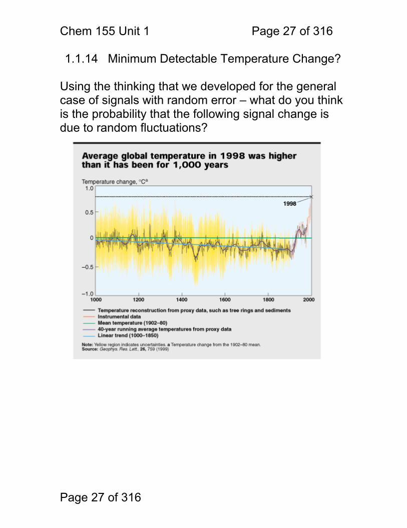
1.1.14 Minimum Detectable Temperature Change? Using the thinking that we developed for the general case of signals with random error – what do you think is the probability that the following signal change is due to random fluctuations?
Chem 155 Unit 1 Page 28 of 316
Page 28 of 316
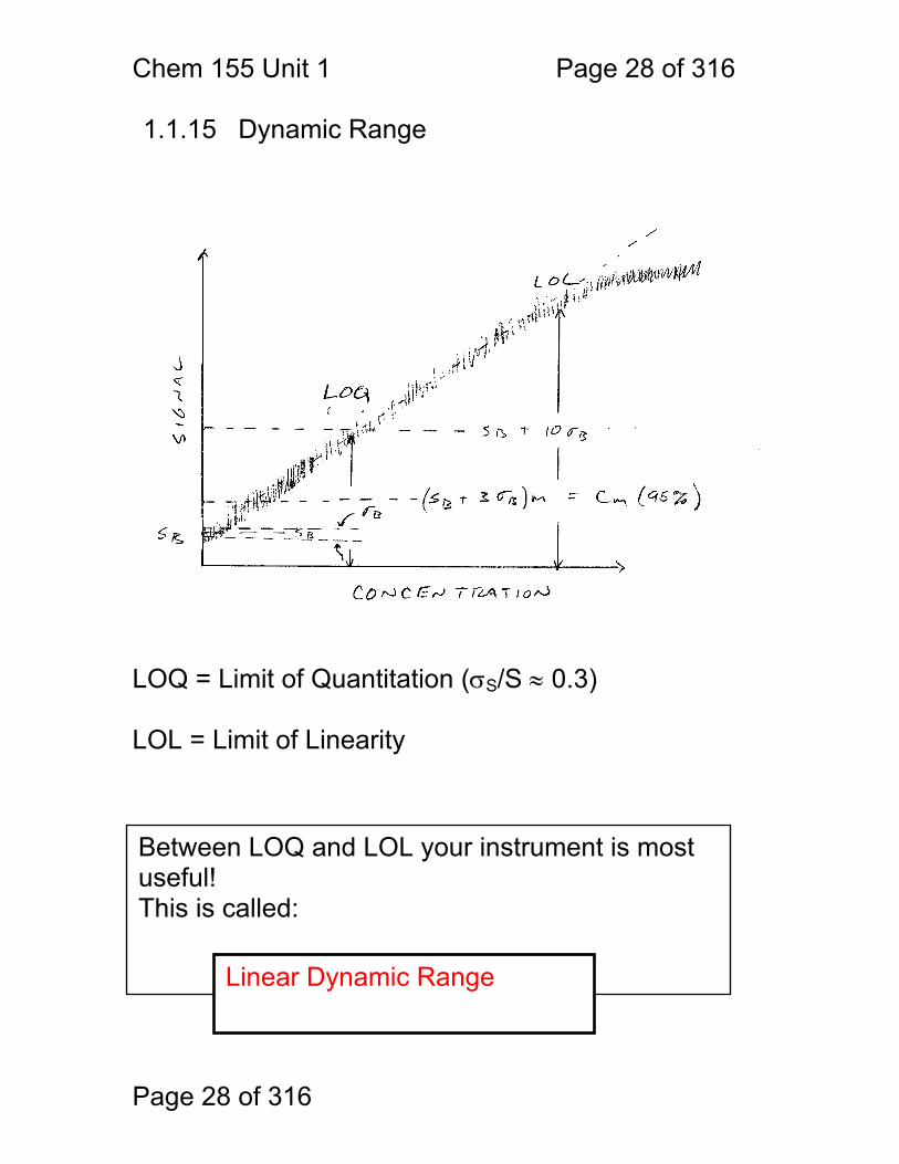
1.1.15 Dynamic Range LOQ = Limit of Quantitation (σS/S ≈ 0.3) LOL = Limit of Linearity
Between LOQ and LOL your instrument is most useful! This is called:
Linear Dynamic Range
Chem 155 Unit 1 Page 29 of 316
Page 29 of 316
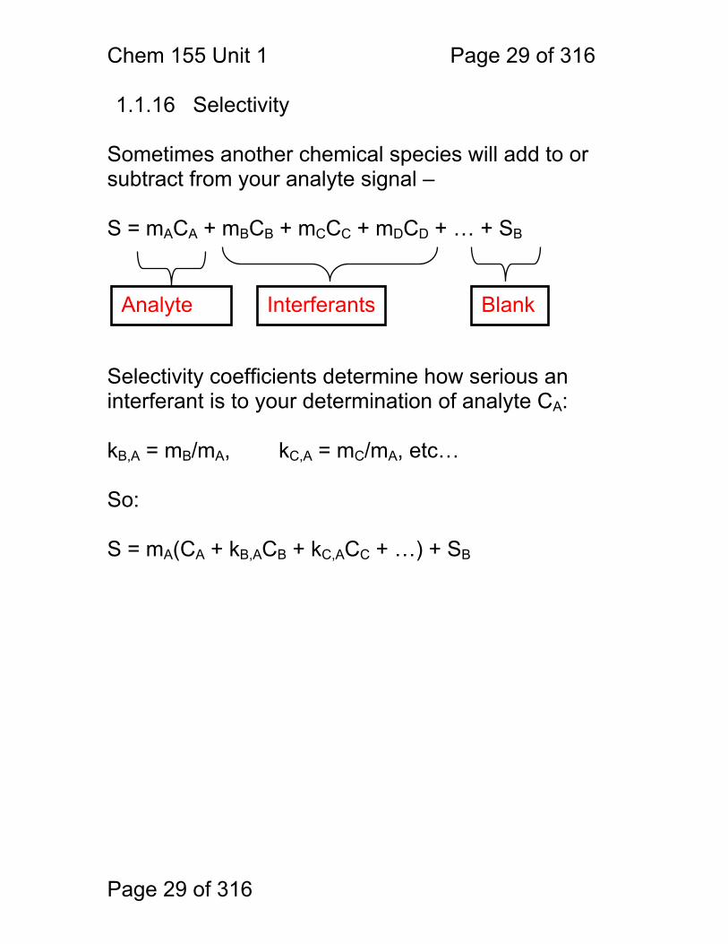
1.1.16 Selectivity Sometimes another chemical species will add to or subtract from your analyte signal – S = mACA + mBCB + mCCC + mDCD + … + SB Selectivity coefficients determine how serious an interferant is to your determination of analyte CA: kB,A = mB/mA, kC,A = mC/mA, etc… So: S = mA(CA + kB,ACB + kC,ACC + …) + SB
Analyte Interferants Blank
Chem 155 Unit 1 Page 30 of 316
Page 30 of 316
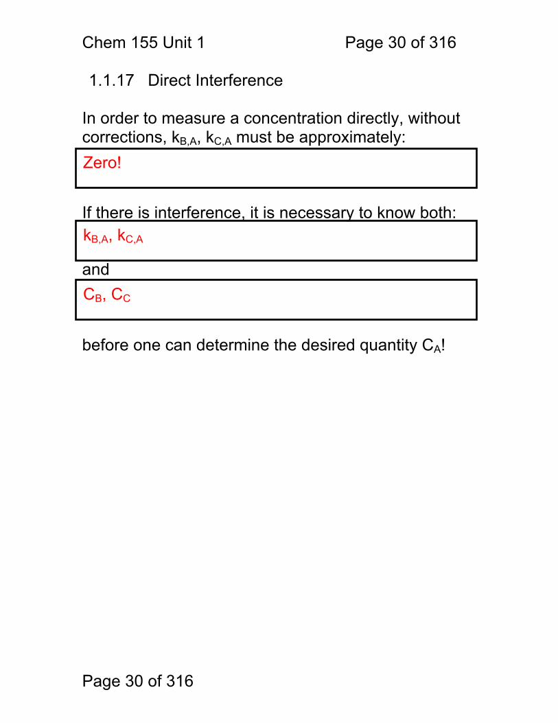
1.1.17 Direct Interference In order to measure a concentration directly, without corrections, kB,A, kC,A must be approximately: If there is interference, it is necessary to know both: and before one can determine the desired quantity CA!
Zero!
kB,A, kC,A
CB, CC
Chem 155 Unit 1 Page 31 of 316
Page 31 of 316
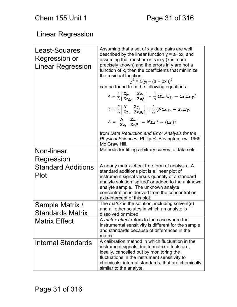
Linear Regression Least-Squares Regression or Linear Regression
Assuming that a set of x,y data pairs are well described by the linear function y = a+bx, and assuming that most error is in y (x is more precisely known) and the errors in y are not a function of x, then the coefficients that minimize the residual function:
χ2 = Σ(yI – (a + bxI))2 can be found from the following equations:
from Data Reduction and Error Analysis for the Physical Sciences, Philip R. Bevington, cw. 1969 Mc Graw Hill.
Non-linear Regression
Methods for fitting arbitrary curves to data sets.
Standard Additions Plot
A nearly matrix-effect free form of analysis. A standard additions plot is a linear plot of instrument signal versus quantity of a standard analyte solution ‘spiked’ or added to the unknown analyte sample. The unknown analyte concentration is derived from the concentration axis-intercept of this plot.
Sample Matrix / Standards Matrix
The matrix is the solution, including solvent(s) and all other solutes in which an analyte is dissolved or mixed
Matrix Effect A matrix effect refers to the case where the instrumental sensitivity is different for the sample and standards because of differences in the matrix.
Internal Standards A calibration method in which fluctuation in the instrument signals due to matrix effects are, ideally, cancelled out by monitoring the fluctuations in the instrument sensitivity to chemicals, internal standards, that are chemically similar to the analyte.

Chem 155 Unit 1 Page 32 of 316
Page 32 of 316
0 2 4 6 8 100
0.5
1
1.5
Analyte Concentration (C)
Inst
rum
ent S
igna
l (S)
1.5
0
Si
Si
FiFi
100 Ci
1.1.18 Linear Least Squares Calibration The most common method for determining the concentration of an unknown analyte is the simple calibration curve. In the calibration curve method, one measures the instrument signal for a range of analyte concentrations (called standards) and develops an approximate relationship (mathematically or graphically) between some signal ‘S’ and analyte concentration ‘C’. If the signal-concentration relationship is linear, then: But, one can not just draw the line between any two points because all the points have some error. So, one mathematically attempts to minimize the residuals.
χ2 = Σ(yi – (a + bxi))2
S = SB + mC y = a + bx
Chem 155 Unit 1 Page 33 of 316
Page 33 of 316
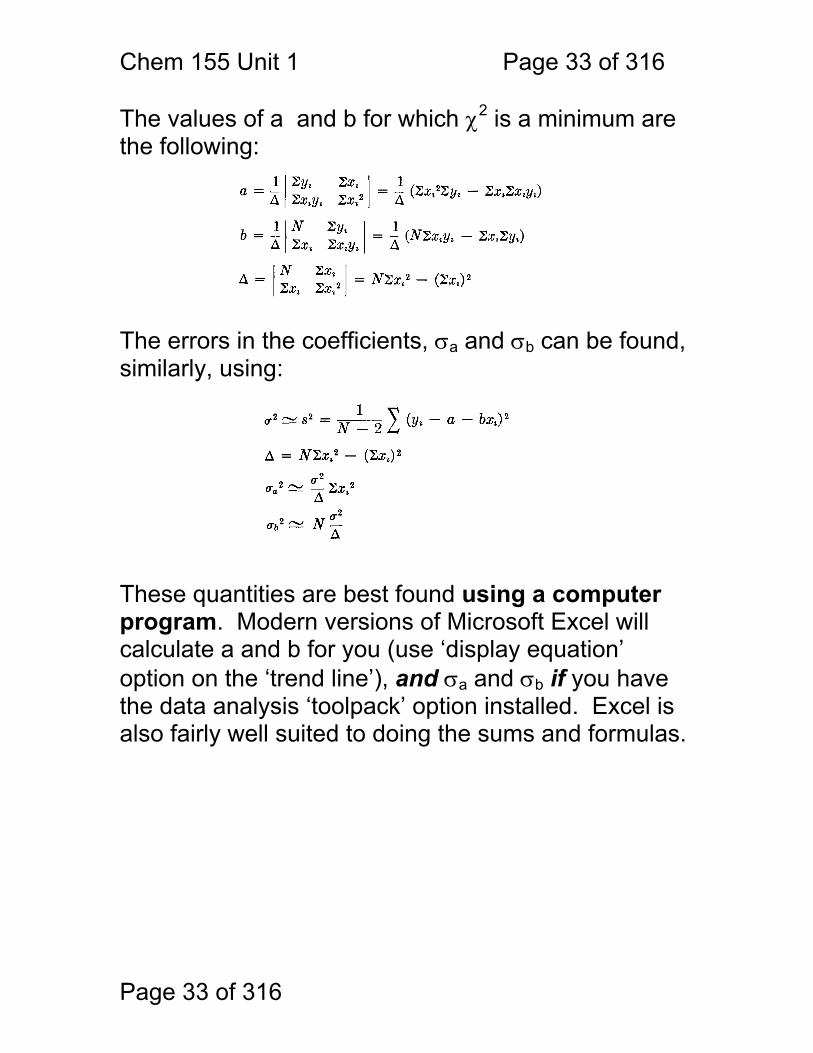
The values of a and b for which χ2 is a minimum are the following: The errors in the coefficients, σa and σb can be found, similarly, using:
These quantities are best found using a computer program. Modern versions of Microsoft Excel will calculate a and b for you (use ‘display equation’ option on the ‘trend line’), and σa and σb if you have the data analysis ‘toolpack’ option installed. Excel is also fairly well suited to doing the sums and formulas.
Chem 155 Unit 1 Page 34 of 316
Page 34 of 316
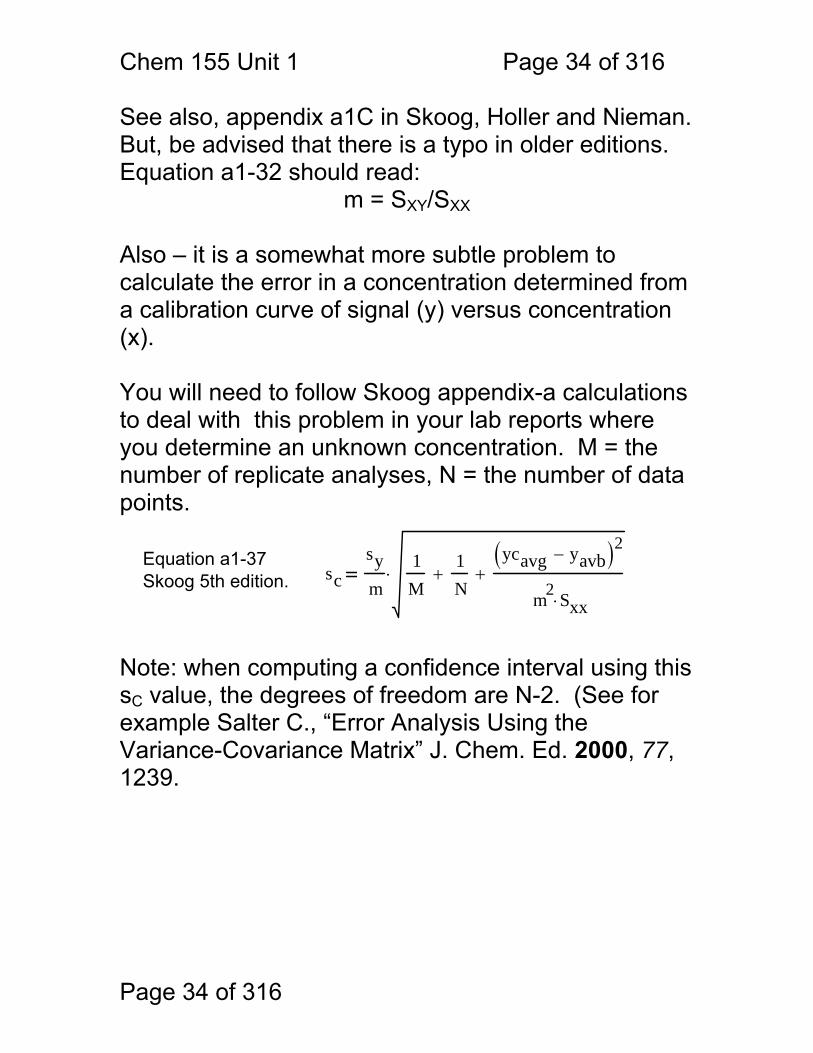
See also, appendix a1C in Skoog, Holler and Nieman. But, be advised that there is a typo in older editions. Equation a1-32 should read:
m = SXY/SXX Also – it is a somewhat more subtle problem to calculate the error in a concentration determined from a calibration curve of signal (y) versus concentration (x). You will need to follow Skoog appendix-a calculations to deal with this problem in your lab reports where you determine an unknown concentration. M = the number of replicate analyses, N = the number of data points. Note: when computing a confidence interval using this sC value, the degrees of freedom are N-2. (See for example Salter C., “Error Analysis Using the Variance-Covariance Matrix” J. Chem. Ed. 2000, 77, 1239.
Equation a1-37Skoog 5th edition. sc
sym
1M
1N
+ycavg yavb−( )2
m2 Sxx⋅+⋅
Chem 155 Unit 1 Page 35 of 316
Page 35 of 316
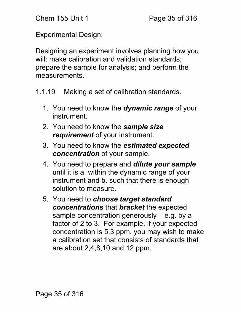
Experimental Design: Designing an experiment involves planning how you will: make calibration and validation standards; prepare the sample for analysis; and perform the measurements. 1.1.19 Making a set of calibration standards.
1. You need to know the dynamic range of your instrument.
2. You need to know the sample size requirement of your instrument.
3. You need to know the estimated expected concentration of your sample.
4. You need to prepare and dilute your sample until it is a. within the dynamic range of your instrument and b. such that there is enough solution to measure.
5. You need to choose target standard concentrations that bracket the expected sample concentration generously – e.g. by a factor of 2 to 3. For example, if your expected concentration is 5.3 ppm, you may wish to make a calibration set that consists of standards that are about 2,4,8,10 and 12 ppm.
Chem 155 Unit 1 Page 36 of 316
Page 36 of 316
6. You need to make a primary stock solution, the concentration of which you know accurately and precisely. This solution will usually be more than twice as concentrated as your most concentrated calibration standard. You will dilute this primary stock solution to make the calibration standards. You need to have enough to make all of your calibration standards.
7. You need to choose the pipets and volumetric flasks that you will use to perform the dilutions. This means that you plan the preparation of each standard. This takes some planning and compromising and many choices – there are many ways to do this correctly – there is more than one right answer!
8. Decide on and record a labeling system in your notebook, collect the glassware, and do the work. I have a labeling system for your caffeine, benzoic acid, iron and zinc standards – I need you to use these labels so that we can sort things out in the class.
Chem 155 Unit 1 Page 37 of 316
Page 37 of 316
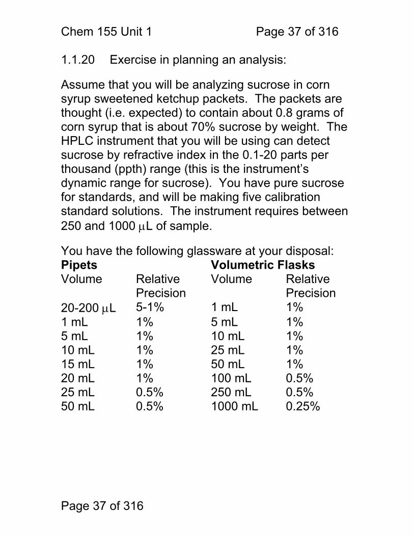
1.1.20 Exercise in planning an analysis: Assume that you will be analyzing sucrose in corn syrup sweetened ketchup packets. The packets are thought (i.e. expected) to contain about 0.8 grams of corn syrup that is about 70% sucrose by weight. The HPLC instrument that you will be using can detect sucrose by refractive index in the 0.1-20 parts per thousand (ppth) range (this is the instrument’s dynamic range for sucrose). You have pure sucrose for standards, and will be making five calibration standard solutions. The instrument requires between 250 and 1000 μL of sample. You have the following glassware at your disposal: Pipets Volumetric Flasks Volume Relative
Precision Volume Relative
Precision 20-200 μL 5-1% 1 mL 1% 1 mL 1% 5 mL 1% 5 mL 1% 10 mL 1% 10 mL 1% 25 mL 1% 15 mL 1% 50 mL 1% 20 mL 1% 100 mL 0.5% 25 mL 0.5% 250 mL 0.5% 50 mL 0.5% 1000 mL 0.25%
Chem 155 Unit 1 Page 38 of 316
Page 38 of 316
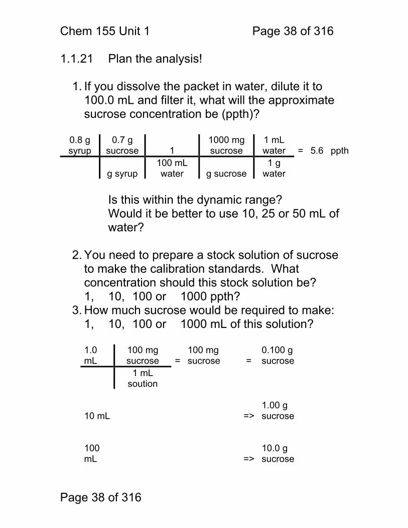
1.1.21 Plan the analysis!
1. If you dissolve the packet in water, dilute it to 100.0 mL and filter it, what will the approximate sucrose concentration be (ppth)?
0.8 g syrup
0.7 g sucrose 1
1000 mg sucrose
1 mL water
= 5.6 ppth
g syrup 100 mL water g sucrose
1 g water
Is this within the dynamic range? Would it be better to use 10, 25 or 50 mL of water?
2. You need to prepare a stock solution of sucrose
to make the calibration standards. What concentration should this stock solution be? 1, 10, 100 or 1000 ppth?
3. How much sucrose would be required to make: 1, 10, 100 or 1000 mL of this solution?
1.0 mL
100 mg sucrose
=
100 mg sucrose =
0.100 g sucrose
1 mL
soution
10 mL =>
1.00 g sucrose
100 mL
=>
10.0 g sucrose
Chem 155 Unit 1 Page 39 of 316
Page 39 of 316
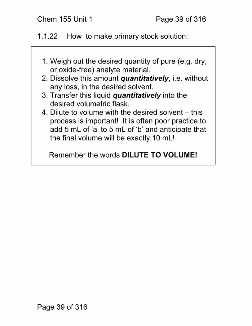
1.1.22 How to make primary stock solution:
1. Weigh out the desired quantity of pure (e.g. dry,
or oxide-free) analyte material. 2. Dissolve this amount quantitatively, i.e. without
any loss, in the desired solvent. 3. Transfer this liquid quantitatively into the
desired volumetric flask. 4. Dilute to volume with the desired solvent – this
process is important! It is often poor practice to add 5 mL of ‘a’ to 5 mL of ‘b’ and anticipate that the final volume will be exactly 10 mL!
Remember the words DILUTE TO VOLUME!
Chem 155 Unit 1 Page 40 of 316
Page 40 of 316
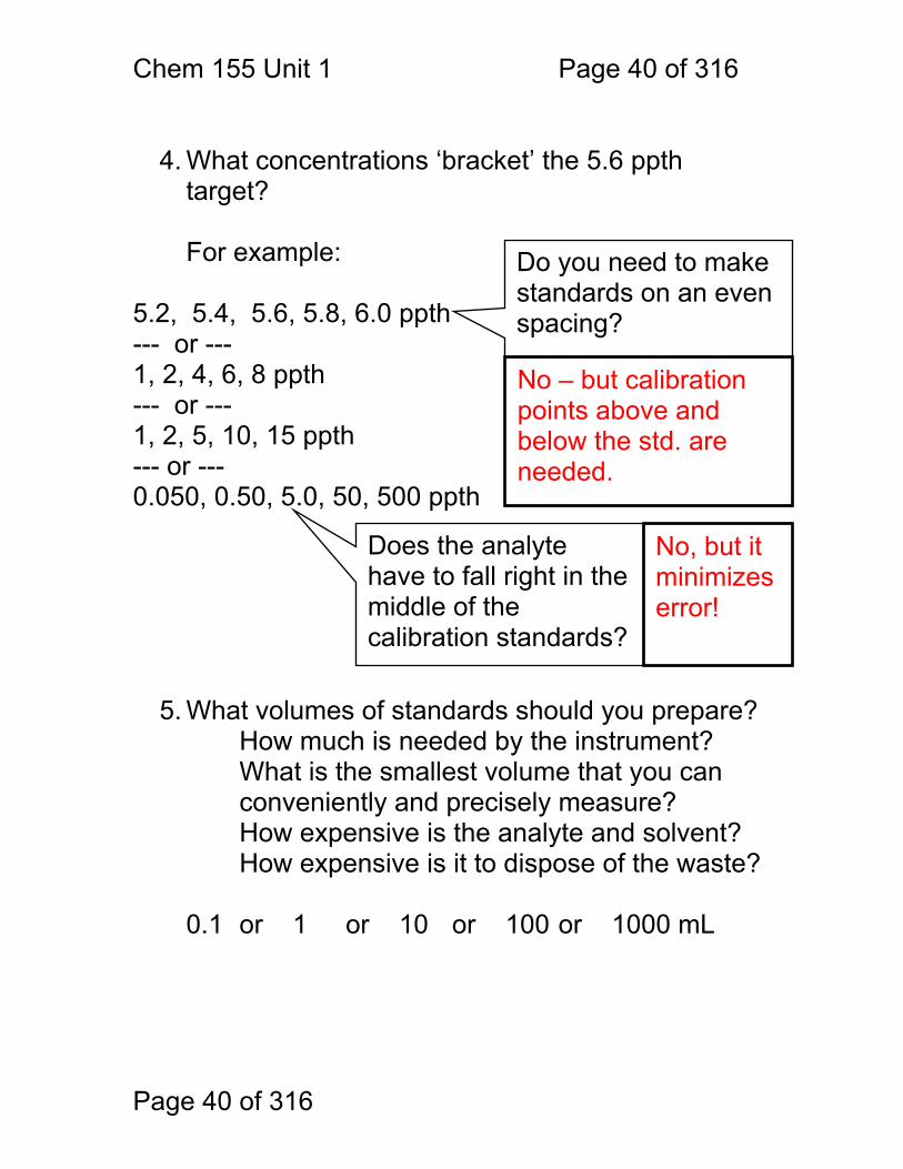
4. What concentrations ‘bracket’ the 5.6 ppth
target? For example:
5.2, 5.4, 5.6, 5.8, 6.0 ppth --- or --- 1, 2, 4, 6, 8 ppth --- or --- 1, 2, 5, 10, 15 ppth --- or --- 0.050, 0.50, 5.0, 50, 500 ppth
5. What volumes of standards should you prepare? How much is needed by the instrument? What is the smallest volume that you can conveniently and precisely measure? How expensive is the analyte and solvent? How expensive is it to dispose of the waste?
0.1 or 1 or 10 or 100 or 1000 mL
Do you need to make standards on an even spacing?
Does the analyte have to fall right in the middle of the calibration standards?
No, but it minimizes error!
No – but calibration points above and below the std. are needed.
Chem 155 Unit 1 Page 41 of 316
Page 41 of 316
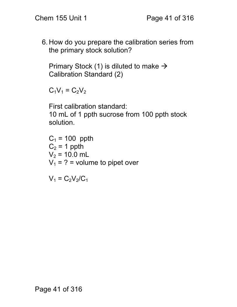
6. How do you prepare the calibration series from
the primary stock solution? Primary Stock (1) is diluted to make Calibration Standard (2) C1V1 = C2V2 First calibration standard: 10 mL of 1 ppth sucrose from 100 ppth stock solution. C1 = 100 ppth C2 = 1 ppth V2 = 10.0 mL V1 = ? = volume to pipet over
V1 = C2V2/C1
Chem 155 Unit 1 Page 42 of 316
Page 42 of 316
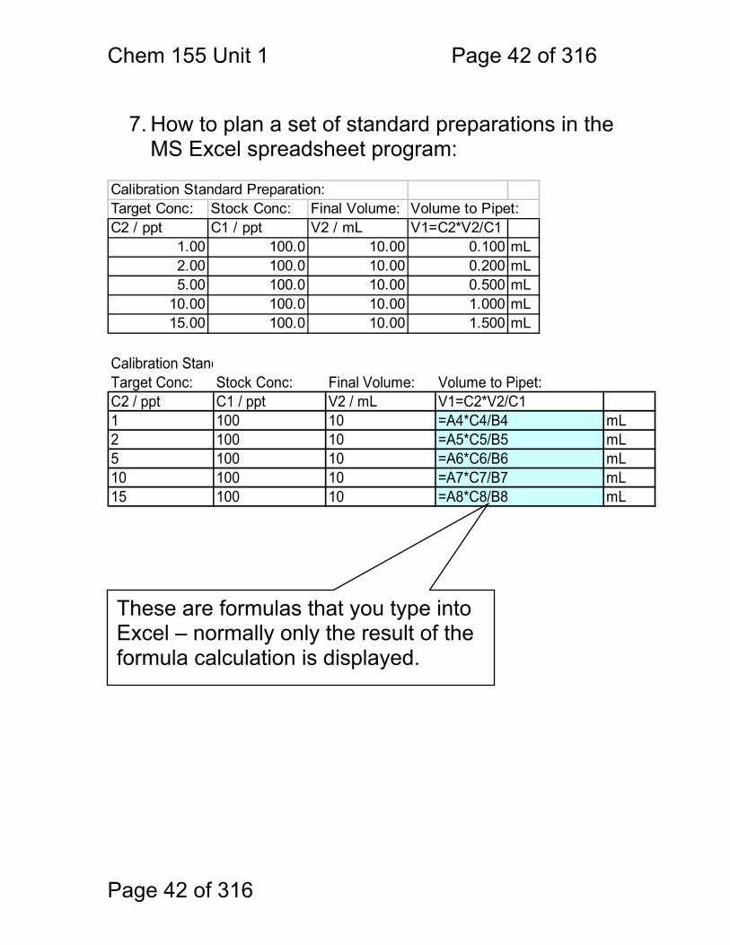
7. How to plan a set of standard preparations in the
MS Excel spreadsheet program: Calibration Standard Preparation:Target Conc: Stock Conc: Final Volume: Volume to Pipet:C2 / ppt C1 / ppt V2 / mL V1=C2*V2/C1
1.00 100.0 10.00 0.100 mL2.00 100.0 10.00 0.200 mL5.00 100.0 10.00 0.500 mL
10.00 100.0 10.00 1.000 mL15.00 100.0 10.00 1.500 mL
Calibration StandTarget Conc: Stock Conc: Final Volume: Volume to Pipet:C2 / ppt C1 / ppt V2 / mL V1=C2*V2/C11 100 10 =A4*C4/B4 mL2 100 10 =A5*C5/B5 mL5 100 10 =A6*C6/B6 mL10 100 10 =A7*C7/B7 mL15 100 10 =A8*C8/B8 mL These are formulas that you type into Excel – normally only the result of the formula calculation is displayed.
Chem 155 Unit 1 Page 43 of 316
Page 43 of 316
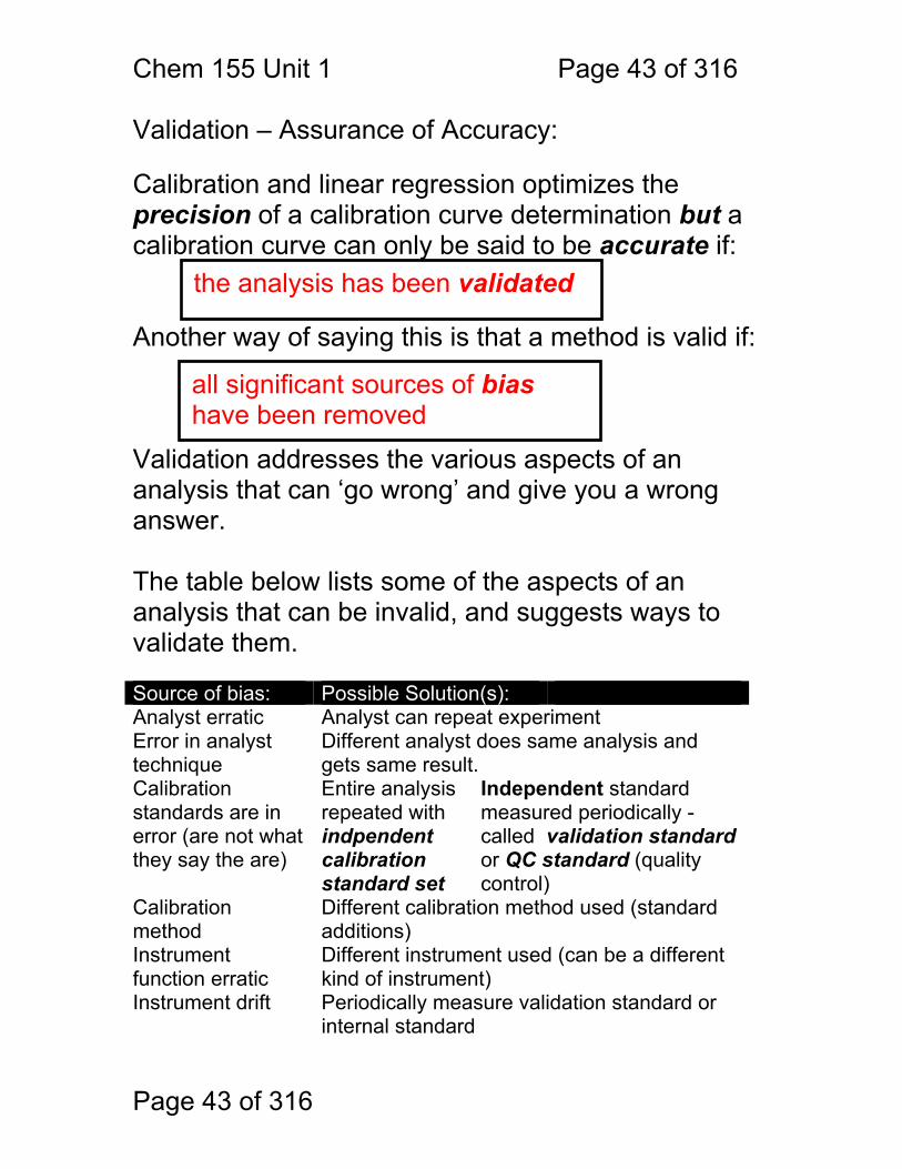
Validation – Assurance of Accuracy: Calibration and linear regression optimizes the precision of a calibration curve determination but a calibration curve can only be said to be accurate if: Another way of saying this is that a method is valid if: Validation addresses the various aspects of an analysis that can ‘go wrong’ and give you a wrong answer. The table below lists some of the aspects of an analysis that can be invalid, and suggests ways to validate them. Source of bias: Possible Solution(s): Analyst erratic Analyst can repeat experiment Error in analyst technique
Different analyst does same analysis and gets same result.
Calibration standards are in error (are not what they say the are)
Entire analysis repeated with indpendent calibration standard set
Independent standard measured periodically - called validation standard or QC standard (quality control)
Calibration method
Different calibration method used (standard additions)
Instrument function erratic
Different instrument used (can be a different kind of instrument)
Instrument drift Periodically measure validation standard or internal standard
the analysis has been validated
all significant sources of bias have been removed
Chem 155 Unit 1 Page 44 of 316
Page 44 of 316
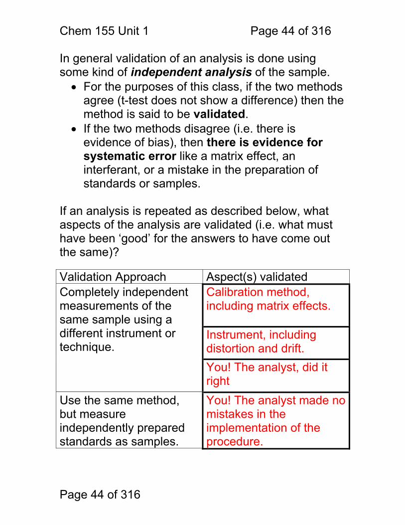
In general validation of an analysis is done using some kind of independent analysis of the sample.
• For the purposes of this class, if the two methods agree (t-test does not show a difference) then the method is said to be validated.
• If the two methods disagree (i.e. there is evidence of bias), then there is evidence for systematic error like a matrix effect, an interferant, or a mistake in the preparation of standards or samples.
If an analysis is repeated as described below, what aspects of the analysis are validated (i.e. what must have been ‘good’ for the answers to have come out the same)? Validation Approach Aspect(s) validated Completely independent measurements of the same sample using a different instrument or technique.
Calibration method, including matrix effects. Instrument, including distortion and drift. You! The analyst, did it right
Use the same method, but measure independently prepared standards as samples.
You! The analyst made no mistakes in the implementation of the procedure.
Chem 155 Unit 1 Page 45 of 316
Page 45 of 316
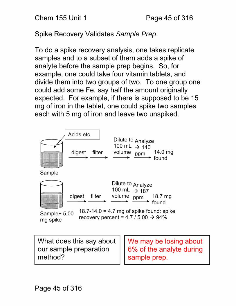
Spike Recovery Validates Sample Prep. To do a spike recovery analysis, one takes replicate samples and to a subset of them adds a spike of analyte before the sample prep begins. So, for example, one could take four vitamin tablets, and divide them into two groups of two. To one group one could add some Fe, say half the amount originally expected. For example, if there is supposed to be 15 mg of iron in the tablet, one could spike two samples each with 5 mg of iron and leave two unspiked.
digest filter
Dilute to 100 mL volume
Sample
Sample+ 5.00 mg spike
Analyze 140
ppm 14.0 mg found
digest filter
Dilute to 100 mL volume
Analyze 187
ppm 18.7 mg found
18.7-14.0 = 4.7 mg of spike found: spike recovery percent = 4.7 / 5.00 94%
Acids etc.
What does this say about our sample preparation method?
We may be losing about 6% of the analyte during sample prep.
Chem 155 Unit 1 Page 46 of 316
Page 46 of 316
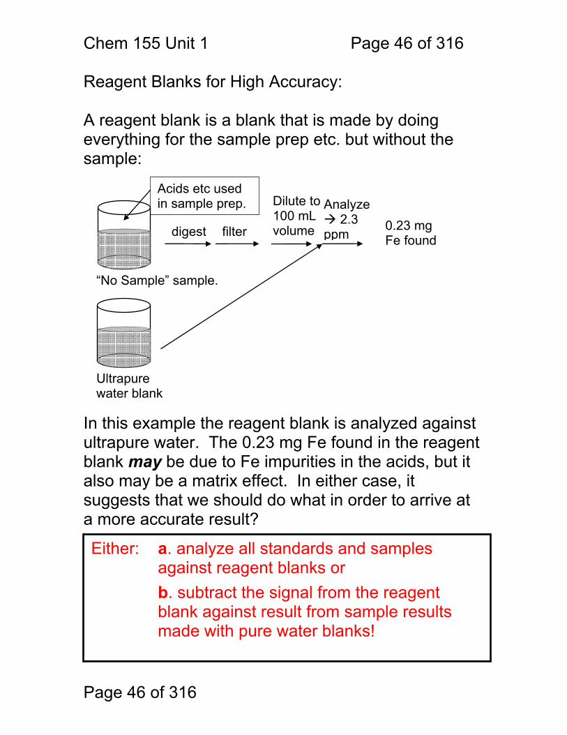
Reagent Blanks for High Accuracy: A reagent blank is a blank that is made by doing everything for the sample prep etc. but without the sample:
In this example the reagent blank is analyzed against ultrapure water. The 0.23 mg Fe found in the reagent blank may be due to Fe impurities in the acids, but it also may be a matrix effect. In either case, it suggests that we should do what in order to arrive at a more accurate result?
digest filter
Dilute to 100 mL volume
“No Sample” sample.
Ultrapure water blank
Analyze 2.3
ppm0.23 mg Fe found
Acids etc used in sample prep.
Either: a. analyze all standards and samples against reagent blanks or b. subtract the signal from the reagent blank against result from sample results made with pure water blanks!
Chem 155 Unit 1 Page 47 of 316
Page 47 of 316
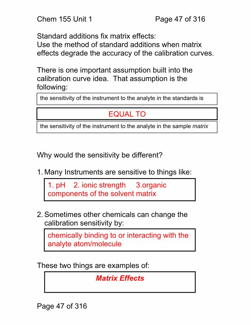
Standard additions fix matrix effects: Use the method of standard additions when matrix effects degrade the accuracy of the calibration curves. There is one important assumption built into the calibration curve idea. That assumption is the following: Why would the sensitivity be different? 1. Many Instruments are sensitive to things like: 2. Sometimes other chemicals can change the
calibration sensitivity by: These two things are examples of:
the sensitivity of the instrument to the analyte in the standards is
the sensitivity of the instrument to the analyte in the sample matrix
EQUAL TO
1. pH 2. ionic strength 3.organic components of the solvent matrix
chemically binding to or interacting with the analyte atom/molecule
Matrix Effects
Chem 155 Unit 1 Page 48 of 316
Page 48 of 316
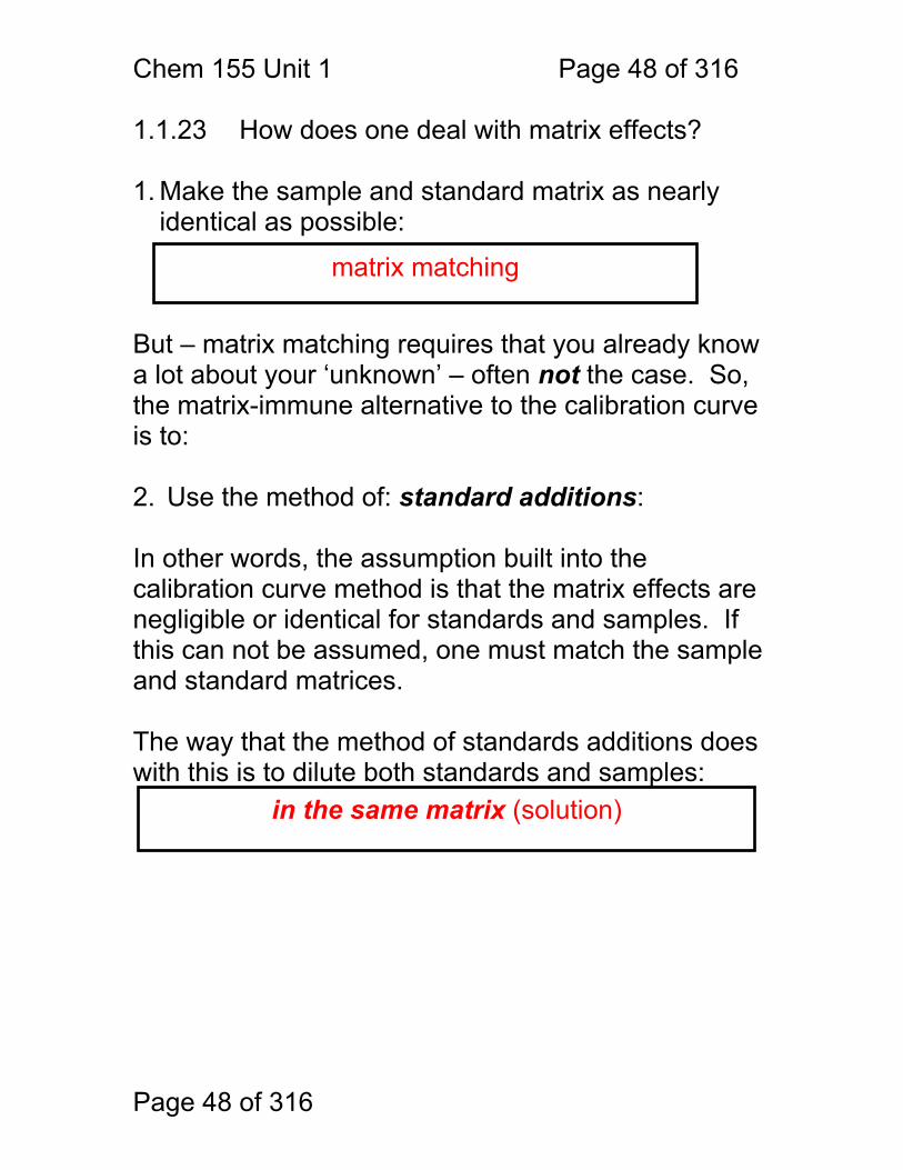
1.1.23 How does one deal with matrix effects? 1. Make the sample and standard matrix as nearly
identical as possible: But – matrix matching requires that you already know a lot about your ‘unknown’ – often not the case. So, the matrix-immune alternative to the calibration curve is to: 2. Use the method of: standard additions: In other words, the assumption built into the calibration curve method is that the matrix effects are negligible or identical for standards and samples. If this can not be assumed, one must match the sample and standard matrices. The way that the method of standards additions does with this is to dilute both standards and samples:
matrix matching
in the same matrix (solution)
Chem 155 Unit 1 Page 49 of 316
Page 49 of 316
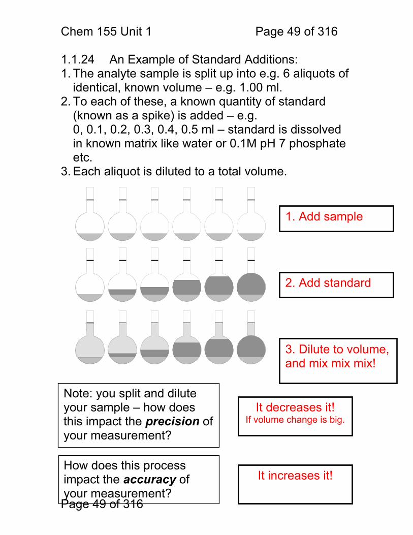
1.1.24 An Example of Standard Additions: 1. The analyte sample is split up into e.g. 6 aliquots of
identical, known volume – e.g. 1.00 ml. 2. To each of these, a known quantity of standard
(known as a spike) is added – e.g. 0, 0.1, 0.2, 0.3, 0.4, 0.5 ml – standard is dissolved in known matrix like water or 0.1M pH 7 phosphate etc.
3. Each aliquot is diluted to a total volume.
Note: you split and dilute your sample – how does this impact the precision of your measurement?
It decreases it! If volume change is big.
How does this process impact the accuracy of your measurement?
It increases it!
3. Dilute to volume, and mix mix mix!
2. Add standard
1. Add sample
Chem 155 Unit 1 Page 50 of 316
Page 50 of 316
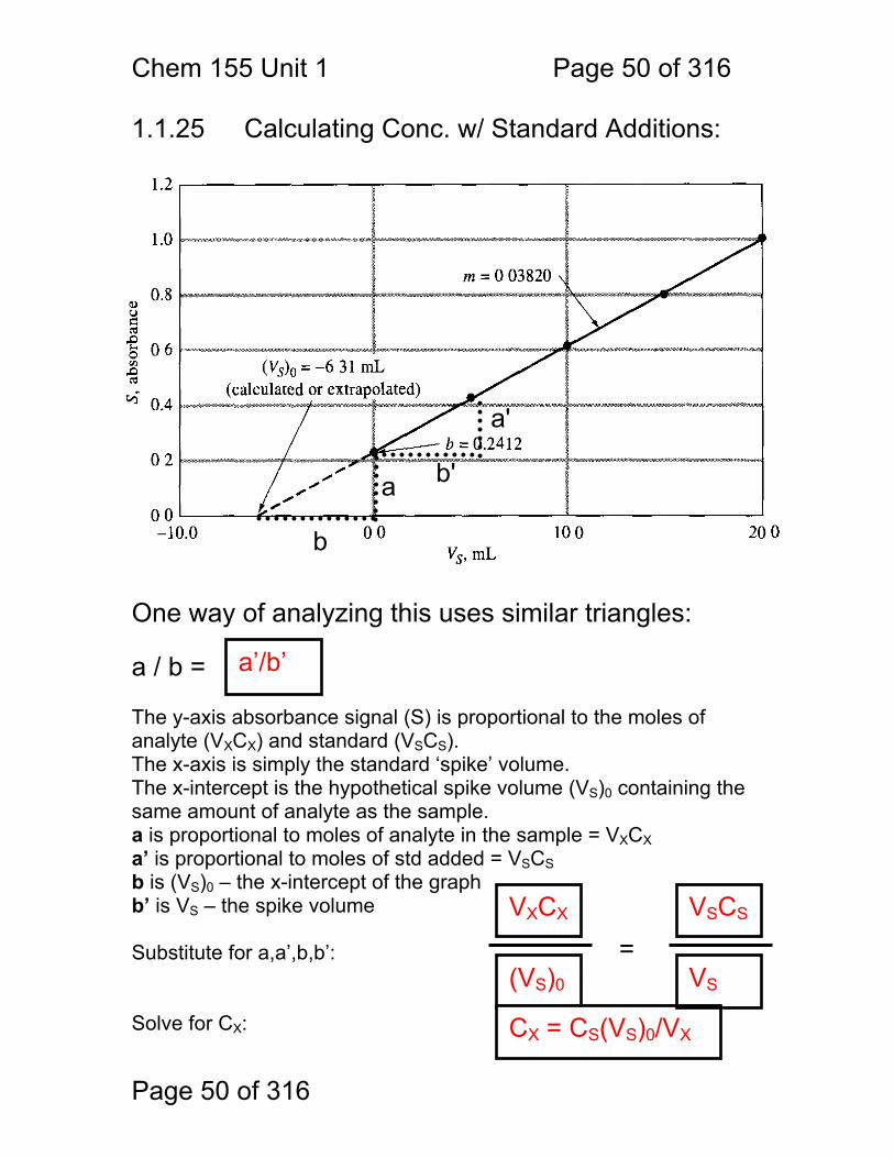
1.1.25 Calculating Conc. w/ Standard Additions: One way of analyzing this uses similar triangles: a / b = The y-axis absorbance signal (S) is proportional to the moles of analyte (VXCX) and standard (VSCS). The x-axis is simply the standard ‘spike’ volume. The x-intercept is the hypothetical spike volume (VS)0 containing the same amount of analyte as the sample. a is proportional to moles of analyte in the sample = VXCX a’ is proportional to moles of std added = VSCS b is (VS)0 – the x-intercept of the graph b’ is VS – the spike volume Substitute for a,a’,b,b’: Solve for CX:
a
b
a'
b'
(VS)0
CX = CS(VS)0/VX
a’/b’
VSCS
= VXCX
VS
Chem 155 Unit 1 Page 51 of 316
Page 51 of 316
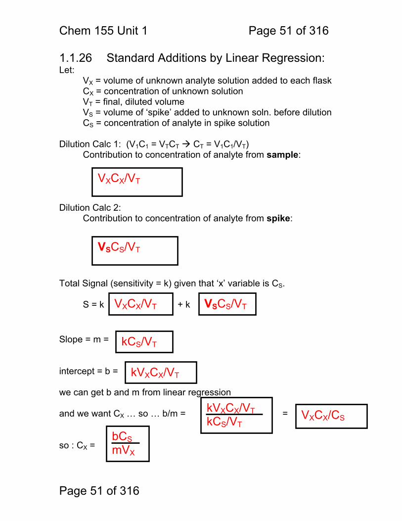
1.1.26 Standard Additions by Linear Regression: Let:
VX = volume of unknown analyte solution added to each flask CX = concentration of unknown solution VT = final, diluted volume VS = volume of ‘spike’ added to unknown soln. before dilution CS = concentration of analyte in spike solution
Dilution Calc 1: (V1C1 = VTCT CT = V1C1/VT)
Contribution to concentration of analyte from sample: Dilution Calc 2:
Contribution to concentration of analyte from spike: Total Signal (sensitivity = k) given that ‘x’ variable is CS. S = k + k Slope = m = intercept = b = we can get b and m from linear regression and we want CX … so … b/m = = so : CX =
VXCX/VT
VSCS/VT
VXCX/VT VSCS/VT
kCS/VT
kVXCX/VT
kVXCX/VT kCS/VT
VXCX/CS
bCS mVX
Chem 155 Unit 1 Page 52 of 316
Page 52 of 316
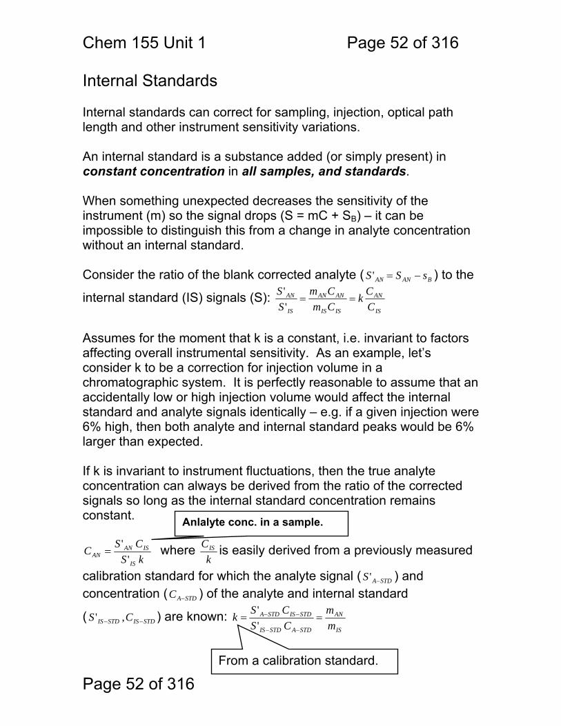
Internal Standards Internal standards can correct for sampling, injection, optical path length and other instrument sensitivity variations. An internal standard is a substance added (or simply present) in constant concentration in all samples, and standards. When something unexpected decreases the sensitivity of the instrument (m) so the signal drops (S = mC + SB) – it can be impossible to distinguish this from a change in analyte concentration without an internal standard. Consider the ratio of the blank corrected analyte ( BANAN sSS −=' ) to the
internal standard (IS) signals (S): IS
AN
ISIS
ANAN
IS
AN
CCk
CmCm
SS
==''
Assumes for the moment that k is a constant, i.e. invariant to factors affecting overall instrumental sensitivity. As an example, let’s consider k to be a correction for injection volume in a chromatographic system. It is perfectly reasonable to assume that an accidentally low or high injection volume would affect the internal standard and analyte signals identically – e.g. if a given injection were 6% high, then both analyte and internal standard peaks would be 6% larger than expected. If k is invariant to instrument fluctuations, then the true analyte concentration can always be derived from the ratio of the corrected signals so long as the internal standard concentration remains constant.
kSCSC
IS
ISANAN '
'= where
kCIS is easily derived from a previously measured
calibration standard for which the analyte signal ( STDAS −' ) and concentration ( STDAC − ) of the analyte and internal standard
( STDISSTDIS CS −− ,' ) are known: IS
AN
STDASTDIS
STDISSTDA
mm
CSCSk ==
−−
−−
''
From a calibration standard.
Anlalyte conc. in a sample.

Chem 155 Unit 1 Page 53 of 316
Page 53 of 316
In other words, if CIS is held constant in all experiments, then the ratio of the analyte to internal standard signals will be independent of instrument sensitivity. When to use an internal standard? When substantial influence on instrument sensitivity is expected due to variation in things like: Sample matrix Temperature Detector sensitivity Injection volume Amplifier (electronics) drift Flow rate An internal standard must:
a. not interfere with your analyte b. ideally have the same dependence on the chemical matrix,
temperature (or other troublesome variable) as the analyte. Consider the ubiquitous ‘salt plate’ IR sampling method. A drop of analyte is sandwiched between two salt plates and this is placed in the IR beam. The path-length is highly variable from experiment to experiment. The signal A = εbC where ε is characteristic of the molecule, b is pathlength and C is concentration. If you are doing an experiment to measure the increase in amide formation versus time by the intensity of the amide bands near 1700 cm-1. You could take samples and measure them periodically, but the variability of the pathlength would distort the results. On the other hand, if all the samples were spiked with the same amount of acetonitrile then the sharp nitrile stretch at 2250 cm-1 could be used as an internal standard.

Chem 155 Unit 1 Page 54 of 316
Page 54 of 316
1.1.27 Internal Standards Example: In HPLC the sample is injected into a flowing stream, and the signal is a peak in a plot of absorbance versus time (a chromatogram). Often the volume of the injection will vary from injection to injection, so the peaks will vary in size! All
0 400 800 1200 1600 2000 2400 2800 3200 3600 40000
0.5
1
time / s
abso
rban
ce
0 400 800 1200 1600 2000 2400 2800 3200 3600 40000
0.5
1
time / s
abso
rban
ce
0 400 800 1200 1600 2000 2400 2800 3200 3600 40000
0.5
1
time / s
abso
rban
ce
Peak 5 is the analyte, a caffeine standard, 25 ppm, 530 mAu.s
Peaks 2, 3 and 4 are other ingredients in the sample.
Chromatogram 1 is a standard. Did the caffeine concentration increase from chromatogram 1 to 2? Did the caffeine concentration increase in chromatogram 1 to 3?
1
2
3
Peak 1 is the internal standard. 100 ppm NaNO3, 480 mAu.s
100 ppm NaNO3, 520 mAu.s
Unknown caffeine conc. 630 mAu.s
Chem 155 Unit 1 Page 55 of 316
Page 55 of 316
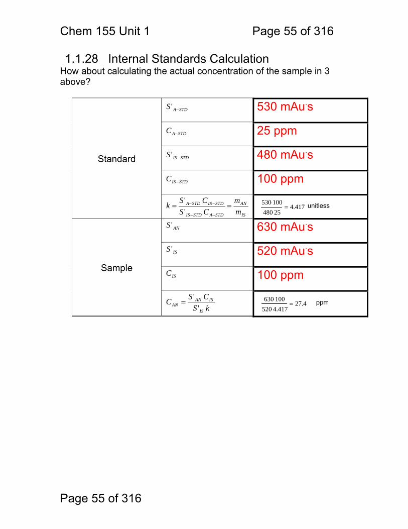
1.1.28 Internal Standards Calculation How about calculating the actual concentration of the sample in 3 above?
Standard
STDAS −' 530 mAu.s
STDAC − 25 ppm
STDISS −' 480 mAu.s
STDISC − 100 ppm
IS
AN
STDASTDIS
STDISSTDA
mm
CSCSk ==
−−
−−
'' 530 100⋅
480 25⋅4.417= unitless
Sample
ANS ' 630 mAu.s
ISS ' 520 mAu.s
ISC 100 ppm
kSCSC
IS
ISANAN '
'= 630 100⋅
520 4.417⋅27.4= ppm
Chem 155 Unit 2 Page 56 of 316
Page 56 of 316
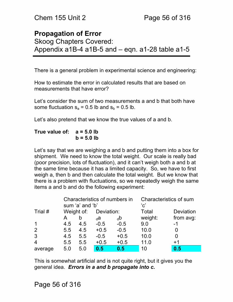
Propagation of Error Skoog Chapters Covered: Appendix a1B-4 a1B-5 and – eqn. a1-28 table a1-5 There is a general problem in experimental science and engineering: How to estimate the error in calculated results that are based on measurements that have error? Let’s consider the sum of two measurements a and b that both have some fluctuation sa = 0.5 lb and sb = 0.5 lb. Let’s also pretend that we know the true values of a and b. True value of: a = 5.0 lb
b = 5.0 lb Let’s say that we are weighing a and b and putting them into a box for shipment. We need to know the total weight. Our scale is really bad (poor precision, lots of fluctuation), and it can’t weigh both a and b at the same time because it has a limited capacity. So, we have to first weigh a, then b and then calculate the total weight. But we know that there is a problem with fluctuations, so we repeatedly weigh the same items a and b and do the following experiment:
Characteristics of numbers in sum ‘a’ and ‘b’
Characteristics of sum ‘c’
Trial # Weight of: Deviation: Total weight:
Deviation from avg: A b da db
1 4.5 4.5 -0.5 -0.5 9.0 -1 2 5.5 4.5 +0.5 -0.5 10.0 0 3 4.5 5.5 -0.5 +0.5 10.0 0 4 5.5 5.5 +0.5 +0.5 11.0 +1 average 5.0 5.0 0.5 0.5 10 0.5 This is somewhat artificial and is not quite right, but it gives you the general idea. Errors in a and b propagate into c.
Chem 155 Unit 2 Page 57 of 316
Page 57 of 316
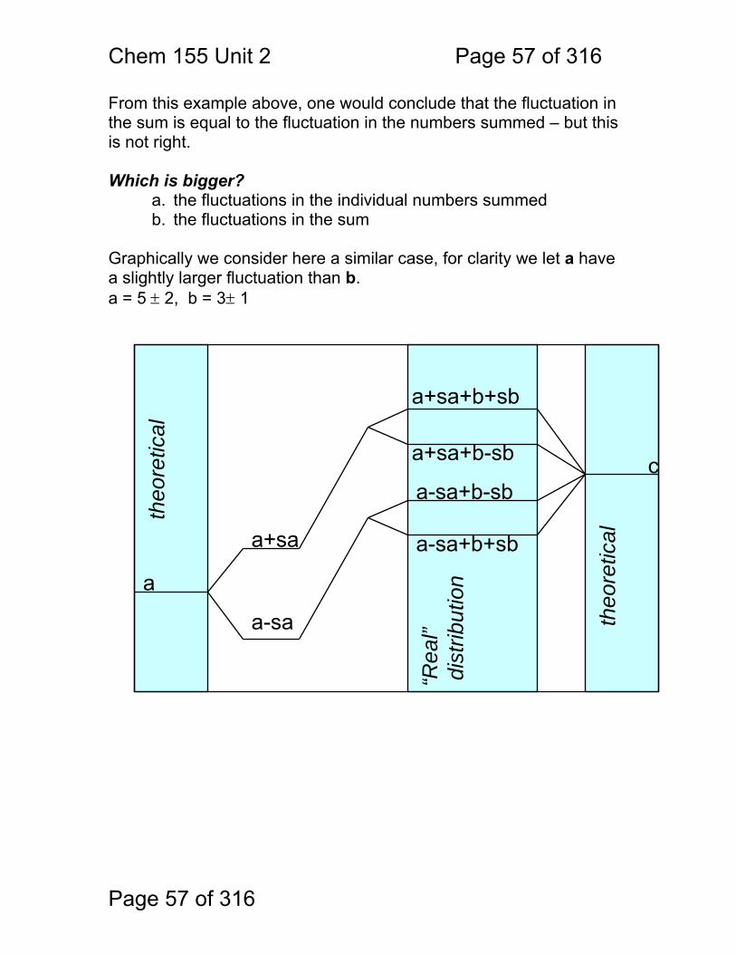
From this example above, one would conclude that the fluctuation in the sum is equal to the fluctuation in the numbers summed – but this is not right. Which is bigger?
a. the fluctuations in the individual numbers summed b. the fluctuations in the sum
Graphically we consider here a similar case, for clarity we let a have a slightly larger fluctuation than b. a = 5 ± 2, b = 3± 1
“Rea
l” d
istri
butio
n
th
eore
tical
th
eore
tical
c
a+sa
a-sa
a+sa+b+sb
a+sa+b-sb
a-sa+b+sb
a-sa+b-sb
a
Chem 155 Unit 2 Page 58 of 316
Page 58 of 316
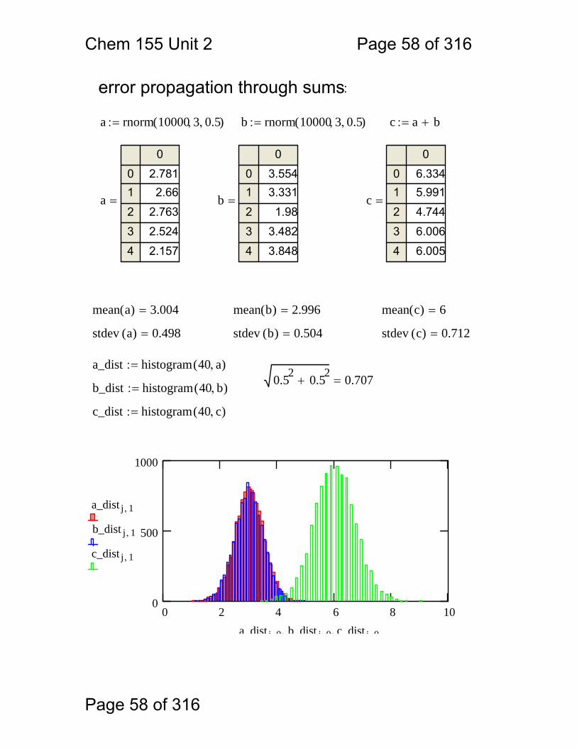
0 2 4 6 8 100
500
1000
a_dist j 1,
b_dist j 1,
c_dist j 1,
a dist j 0 b dist j 0, c dist j 0,
c_dist histogram 40 c,( ):=
b_dist histogram 40 b,( ):=0.52 0.52
+ 0.707=a_dist histogram 40 a,( ):=
stdev c( ) 0.712=stdev b( ) 0.504=stdev a( ) 0.498=
mean c( ) 6=mean b( ) 2.996=mean a( ) 3.004=
c
0
01
2
3
4
6.3345.991
4.744
6.006
6.005
=b
0
01
2
3
4
3.5543.331
1.98
3.482
3.848
=a
0
01
2
3
4
2.7812.66
2.763
2.524
2.157
=
c a b+:=b rnorm 10000 3, 0.5,( ):=a rnorm 10000 3, 0.5,( ):=
error propagation through sums:
Chem 155 Unit 2 Page 59 of 316
Page 59 of 316
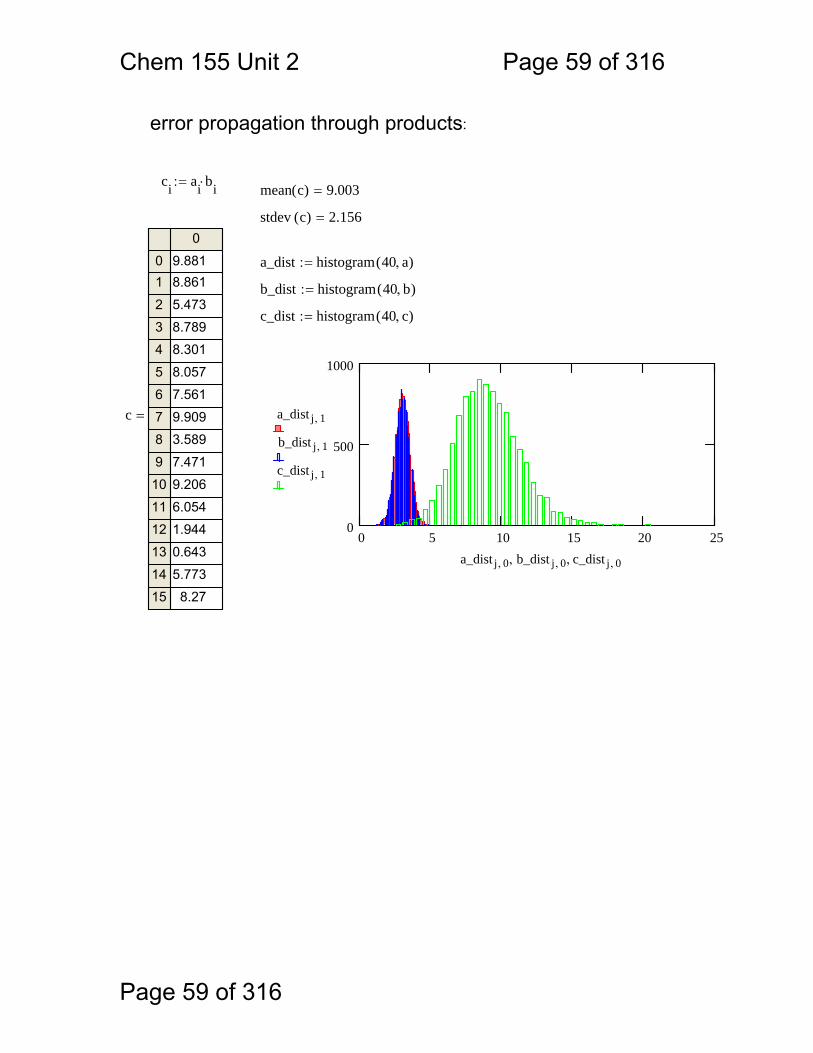
error propagation through products:
ci ai bi⋅:= mean c( ) 9.003=
stdev c( ) 2.156=
a_dist histogram 40 a,( ):=
b_dist histogram 40 b,( ):=
c_dist histogram 40 c,( ):=
0 5 10 15 20 250
500
1000
a_dist j 1,
b_dist j 1,
c_dist j 1,
a_dist j 0, b_dist j 0,, c_dist j 0,,
c
0
01
2
34
5
6
78
9
10
1112
13
1415
9.8818.861
5.473
8.7898.301
8.057
7.561
9.9093.589
7.471
9.206
6.0541.944
0.643
5.7738.27
=
Chem 155 Unit 2 Page 60 of 316
Page 60 of 316
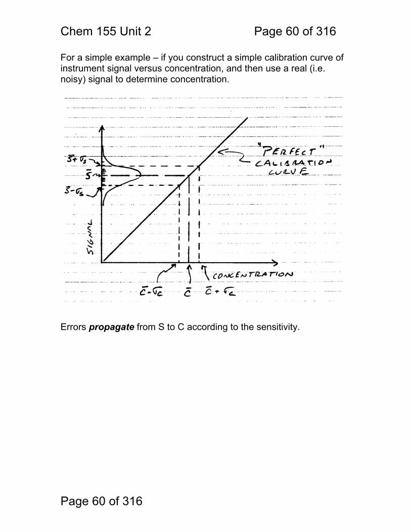
For a simple example – if you construct a simple calibration curve of instrument signal versus concentration, and then use a real (i.e. noisy) signal to determine concentration.
Errors propagate from S to C according to the sensitivity.
Chem 155 Unit 2 Page 61 of 316
Page 61 of 316
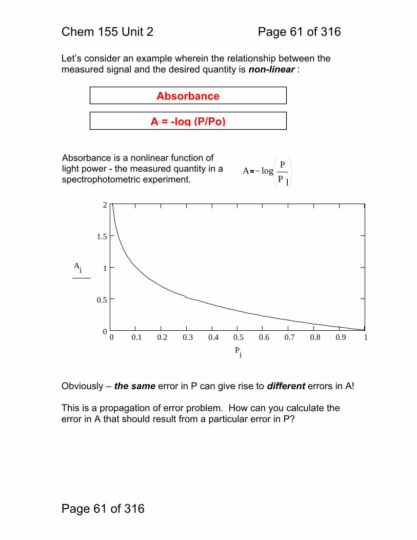
Let’s consider an example wherein the relationship between the measured signal and the desired quantity is non-linear :
Obviously – the same error in P can give rise to different errors in A! This is a propagation of error problem. How can you calculate the error in A that should result from a particular error in P?
Absorbance
Absorbance is a nonlinear function of light power - the measured quantity in a spectrophotometric experiment.
A logPP l
0 0.1 0.2 0.3 0.4 0.5 0.6 0.7 0.8 0.9 10
0.5
1
1.5
2
Ai
Pi
A = -log (P/Po)
Chem 155 Unit 2 Page 62 of 316
Page 62 of 316
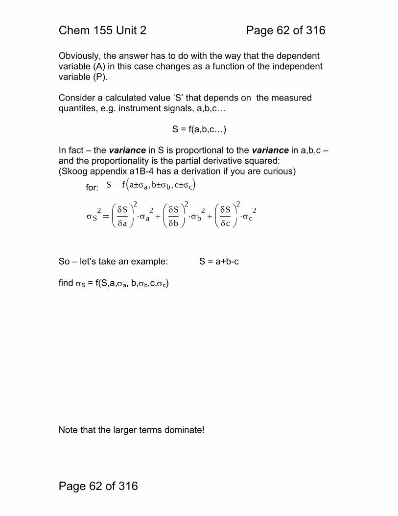
Obviously, the answer has to do with the way that the dependent variable (A) in this case changes as a function of the independent variable (P). Consider a calculated value ‘S’ that depends on the measured quantites, e.g. instrument signals, a,b,c…
S = f(a,b,c…) In fact – the variance in S is proportional to the variance in a,b,c – and the proportionality is the partial derivative squared: (Skoog appendix a1B-4 has a derivation if you are curious)
So – let’s take an example: S = a+b-c find σS = f(S,a,σa, b,σb,c,σc) Note that the larger terms dominate!
S f a±σa b±σb, c±σc,( )for:
σS2 δS
δa⎛⎜⎝
⎞⎟⎠
2σa
2⋅
δSδb
⎛⎜⎝
⎞⎟⎠
2σb
2⋅+
δSδc
⎛⎜⎝
⎞⎟⎠
2σc
2⋅+

Chem 155 Unit 2 Page 63 of 316
Page 63 of 316
Exercise: Prove the “multiplication / division rule” Show that for S = a*b/c
σ S2
S2
σ a2
a2
σ b2
b2
σ c2
c2
Chem 155 Unit 2 Page 64 of 316
Page 64 of 316
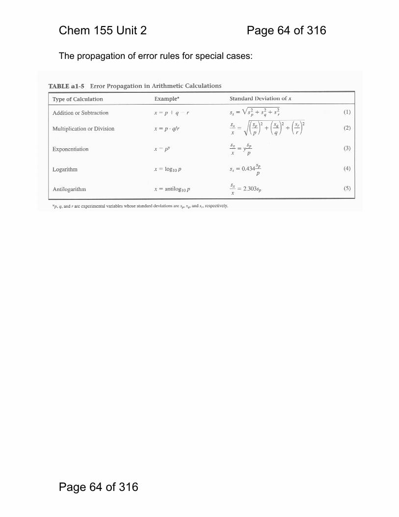
The propagation of error rules for special cases:
Chem 155 Unit 3 Page 65 of 316
Page 65 of 316
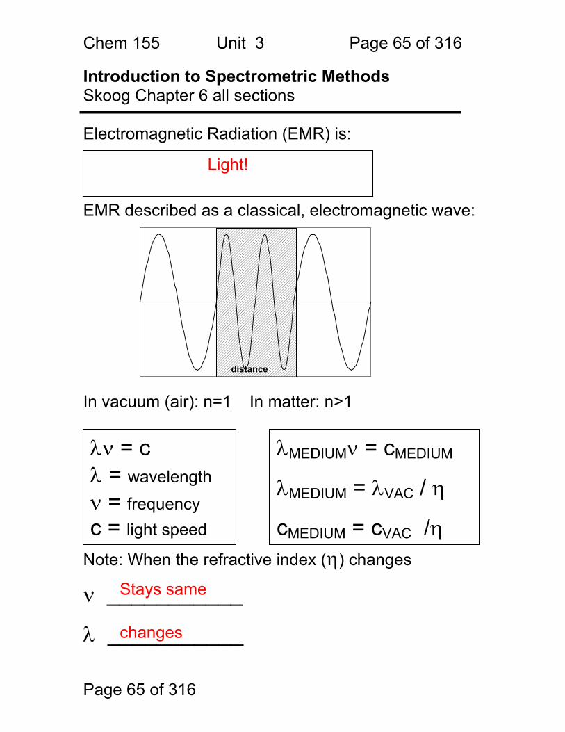
Introduction to Spectrometric Methods Skoog Chapter 6 all sections Electromagnetic Radiation (EMR) is: EMR described as a classical, electromagnetic wave: In vacuum (air): n=1 In matter: n>1 Note: When the refractive index (η) changes
ν ___________
λ ___________
Light!
λν = c λ = wavelength ν = frequency c = light speed
λMEDIUMν = cMEDIUM
λMEDIUM = λVAC / η
cMEDIUM = cVAC /η
distance
Stays same
changes
Chem 155 Unit 3 Page 66 of 316
Page 66 of 316
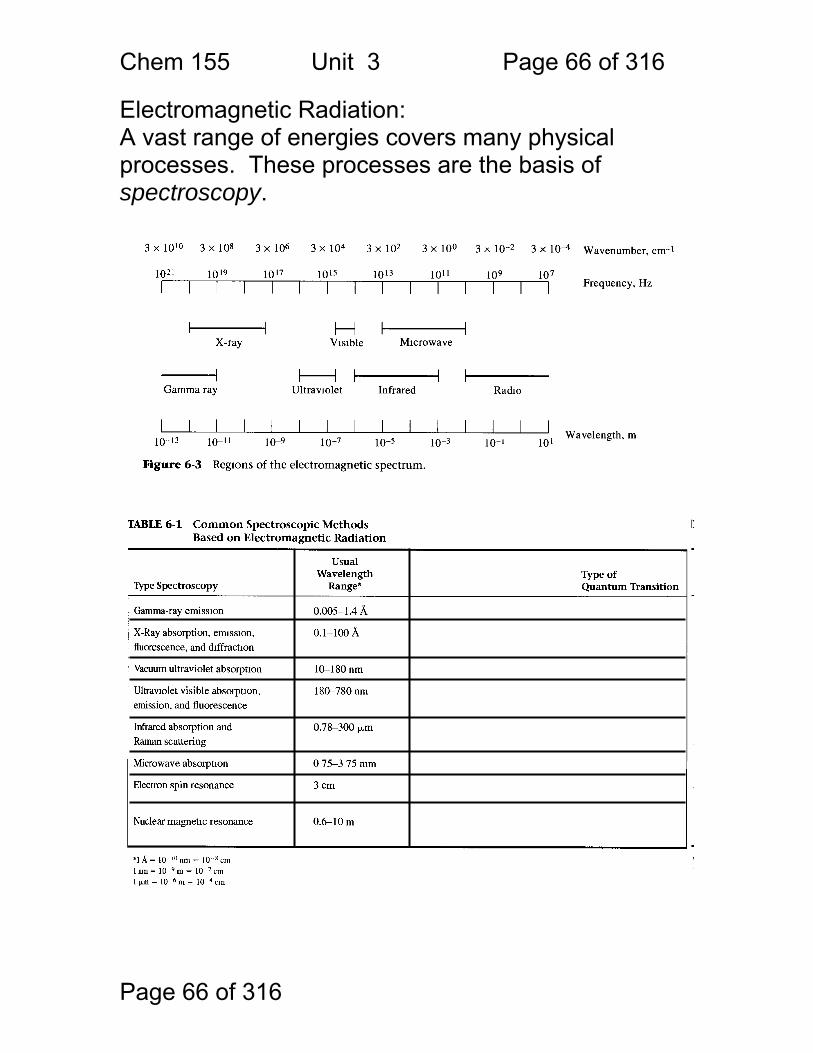
Electromagnetic Radiation: A vast range of energies covers many physical processes. These processes are the basis of spectroscopy.
Chem 155 Unit 3 Page 67 of 316
Page 67 of 316
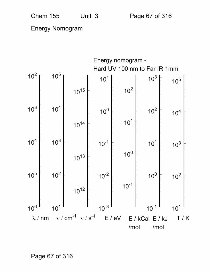
Energy Nomogram
106
105
104
103
102
1012
1013
1014
1015
101
102
103
104
105
10-3
10-2
10-1
100
101
10-1
100
101
102
10-1
100
101
102
103
101
102
103
104
105
λ / nm ν / cm-1 ν / s−1 E / eV E / kCal/mol
T / KE / kJ/mol
Energy nomogram - Hard UV 100 nm to Far IR 1mm
Chem 155 Unit 3 Page 68 of 316
Page 68 of 316
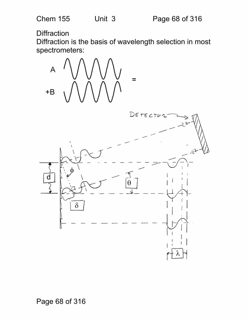
Diffraction Diffraction is the basis of wavelength selection in most spectrometers:
δ
φ
θd
λ
Chem 155 Unit 3 Page 69 of 316
Page 69 of 316
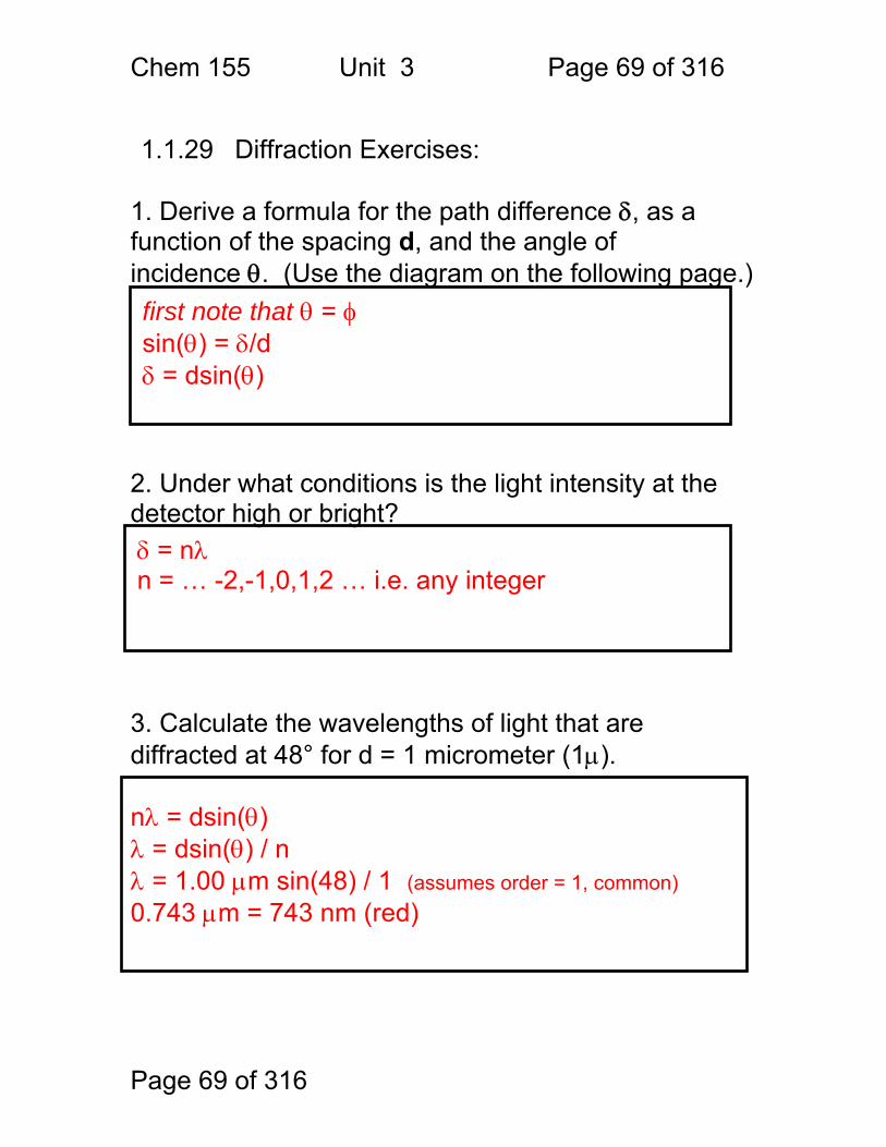
1.1.29 Diffraction Exercises:
1. Derive a formula for the path difference δ, as a function of the spacing d, and the angle of incidence θ. (Use the diagram on the following page.) 2. Under what conditions is the light intensity at the detector high or bright? 3. Calculate the wavelengths of light that are diffracted at 48° for d = 1 micrometer (1μ). nλ = dsin(θ) λ = dsin(θ) / n λ = 1.00 μm sin(48) / 1 (assumes order = 1, common) 0.743 μm = 743 nm (red)
δ = nλ n = … -2,-1,0,1,2 … i.e. any integer
first note that θ = φ sin(θ) = δ/d δ = dsin(θ)
Chem 155 Unit 3 Page 70 of 316
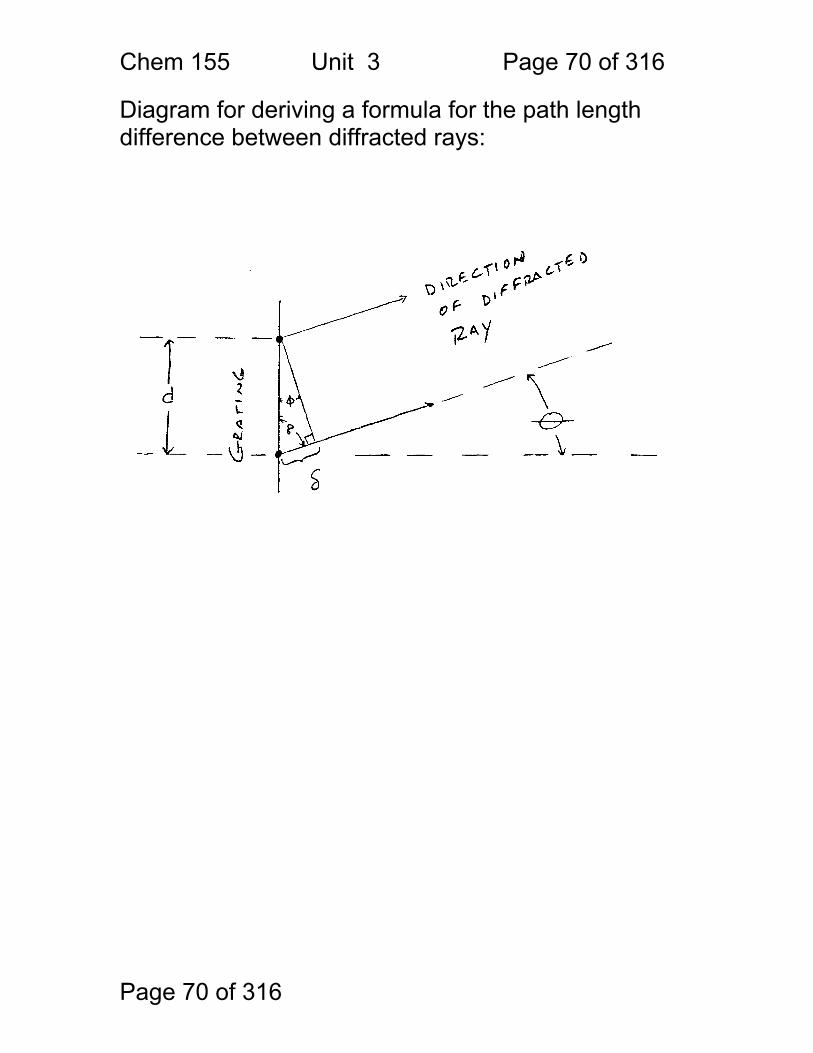
Page 70 of 316
Diagram for deriving a formula for the path length difference between diffracted rays:
Chem 155 Unit 3 Page 71 of 316
Page 71 of 316
Properties of Electromagnetic Radiation: Most EM Radiation is polychromatic, i.e. the beam is a mixture of rays of different: E.g. incandescent light sources are polychromatic. Another term for polychromatic light: is white light. EM Radiation is monochromatic if all rays have identical: E.g. Na-atomic emission lamps are nearly monochromatic because nearly all of the light is from a single atomic transition that emits at 590nm. White light can be filtered so that it is nearly monochromatic. Coherence: EM Radiation is coherent if all rays have identical: Coherent radiation comes from lasers and exotic light sources called synchrotrons.
frequency phase
wavelength
frequencies phases
Chem 155 Unit 3 Page 72 of 316
Page 72 of 316
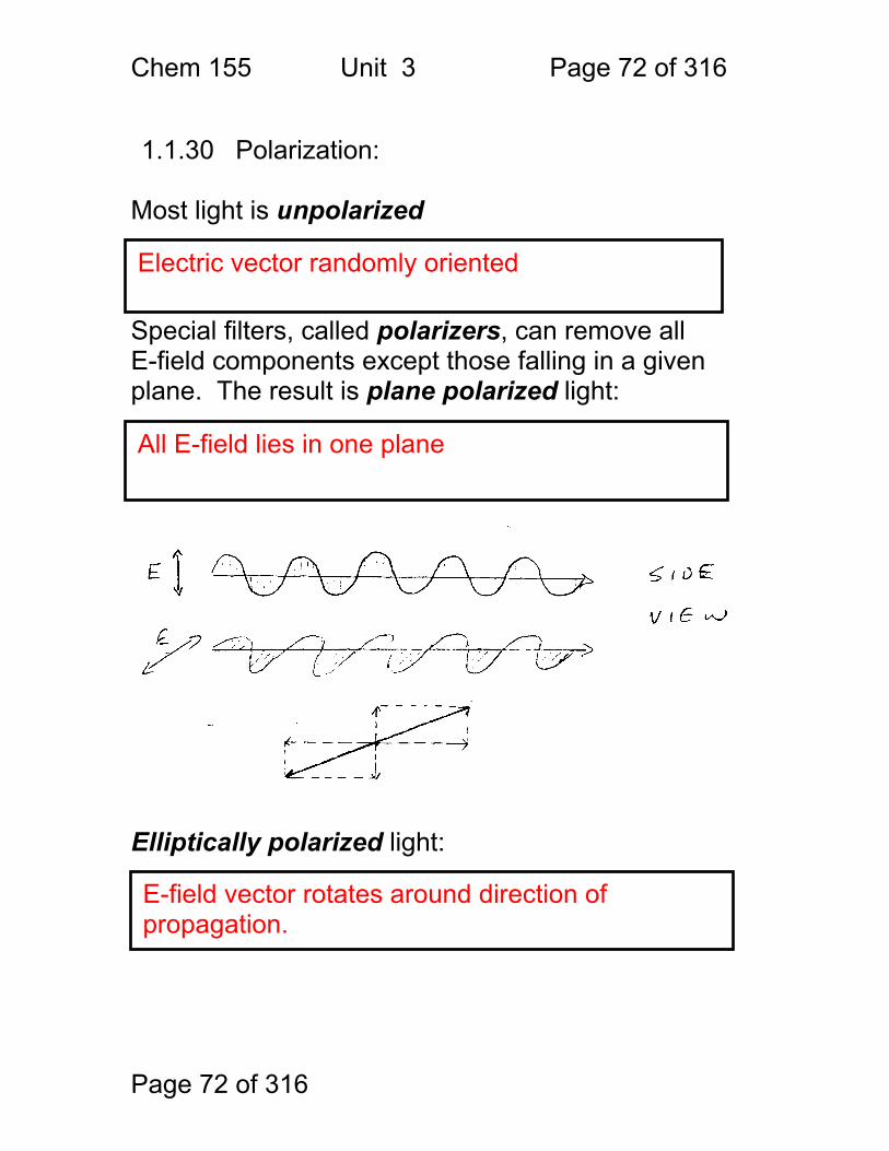
1.1.30 Polarization:
Most light is unpolarized Special filters, called polarizers, can remove all E-field components except those falling in a given plane. The result is plane polarized light: Elliptically polarized light:
Electric vector randomly oriented
All E-field lies in one plane
E-field vector rotates around direction of propagation.
Chem 155 Unit 3 Page 73 of 316
Page 73 of 316
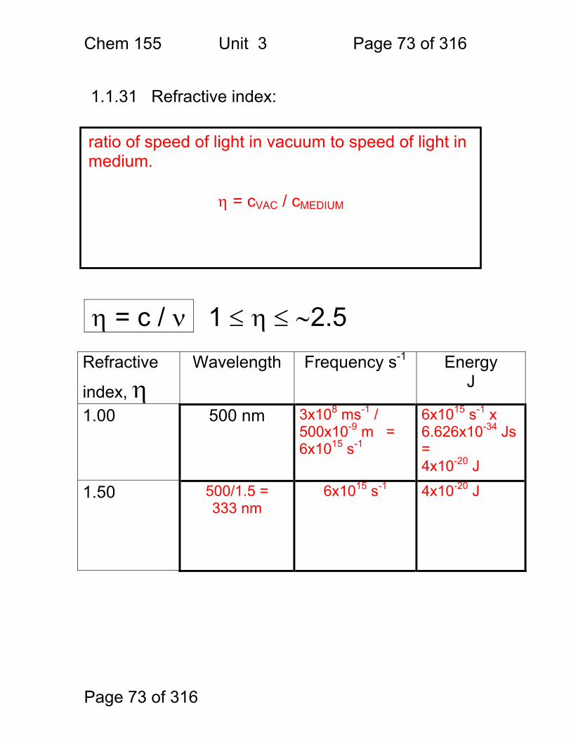
1.1.31 Refractive index:
η = c / ν 1 ≤ η ≤ ∼2.5 Refractive
index, η
Wavelength Frequency s-1 Energy J
1.00 500 nm 3x10⁸ ms-1 / 500x10-9 m = 6x10¹⁵ s-1
6x10¹⁵ s-1 x 6.626x10-34 Js = 4x10-20 J
1.50 500/1.5 = 333 nm
6x10¹⁵ s-1 4x10-20 J
ratio of speed of light in vacuum to speed of light in medium.
η = cVAC / cMEDIUM
Chem 155 Unit 3 Page 74 of 316
Page 74 of 316
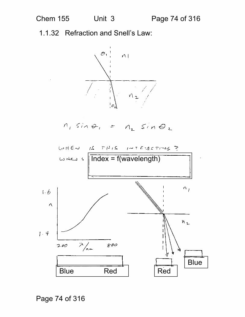
1.1.32 Refraction and Snell’s Law:
Index = f(wavelength)
Blue Red Red Blue
Chem 155 Unit 3 Page 75 of 316
Page 75 of 316
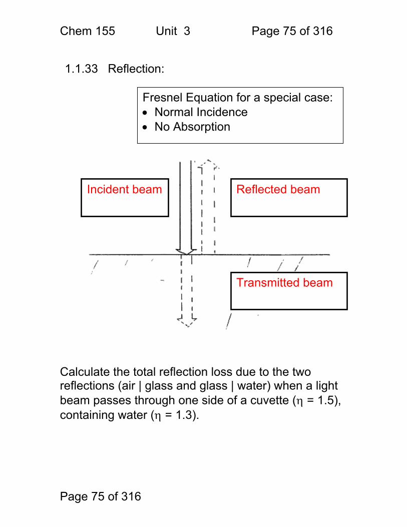
1.1.33 Reflection:
Calculate the total reflection loss due to the two reflections (air | glass and glass | water) when a light beam passes through one side of a cuvette (η = 1.5), containing water (η = 1.3).
Fresnel Equation for a special case: • Normal Incidence • No Absorption
Incident beam Reflected beam
Transmitted beam
Chem 155 Unit 3 Page 76 of 316
Page 76 of 316
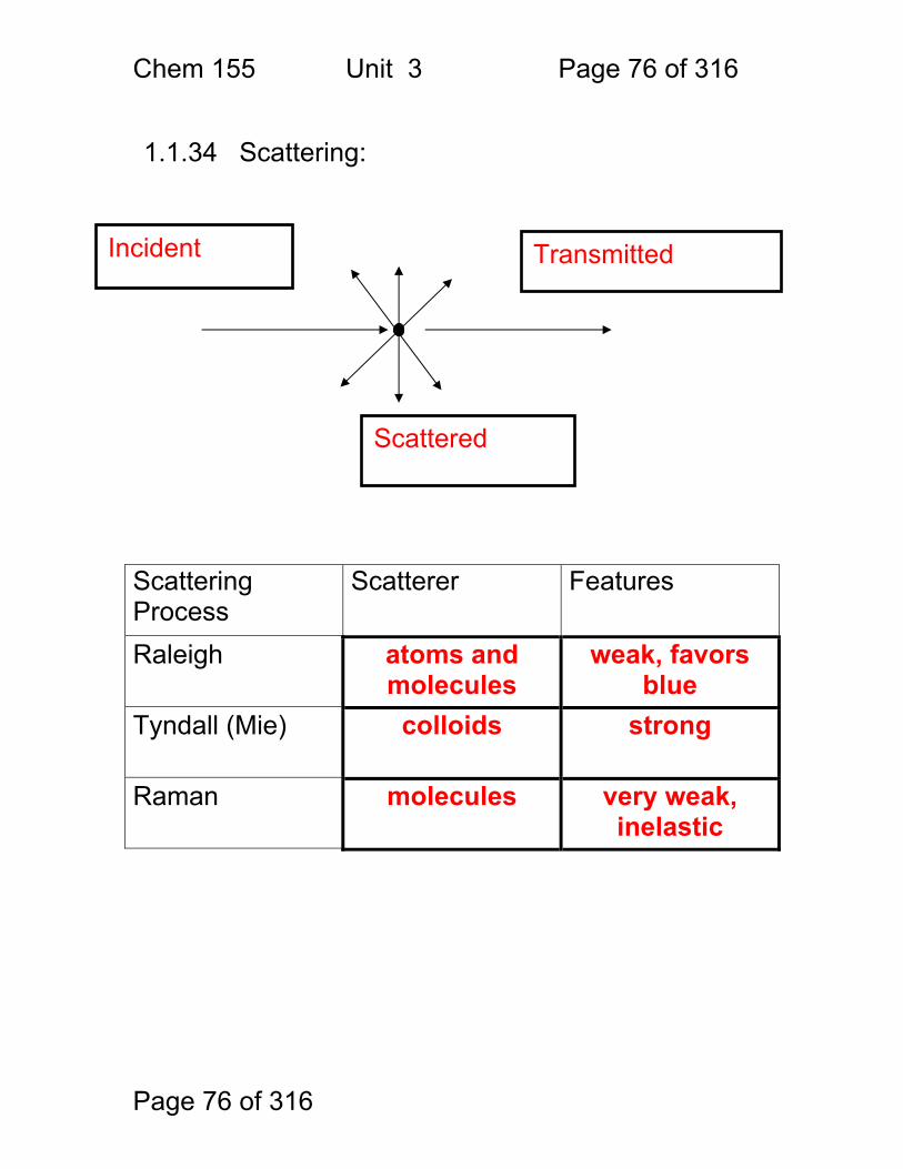
1.1.34 Scattering:
Scattering Process
Scatterer Features
Raleigh atoms and molecules
weak, favors blue
Tyndall (Mie) colloids strong
Raman molecules very weak, inelastic
Incident
Scattered
Transmitted
Chem 155 Unit 3 Page 77 of 316
Page 77 of 316
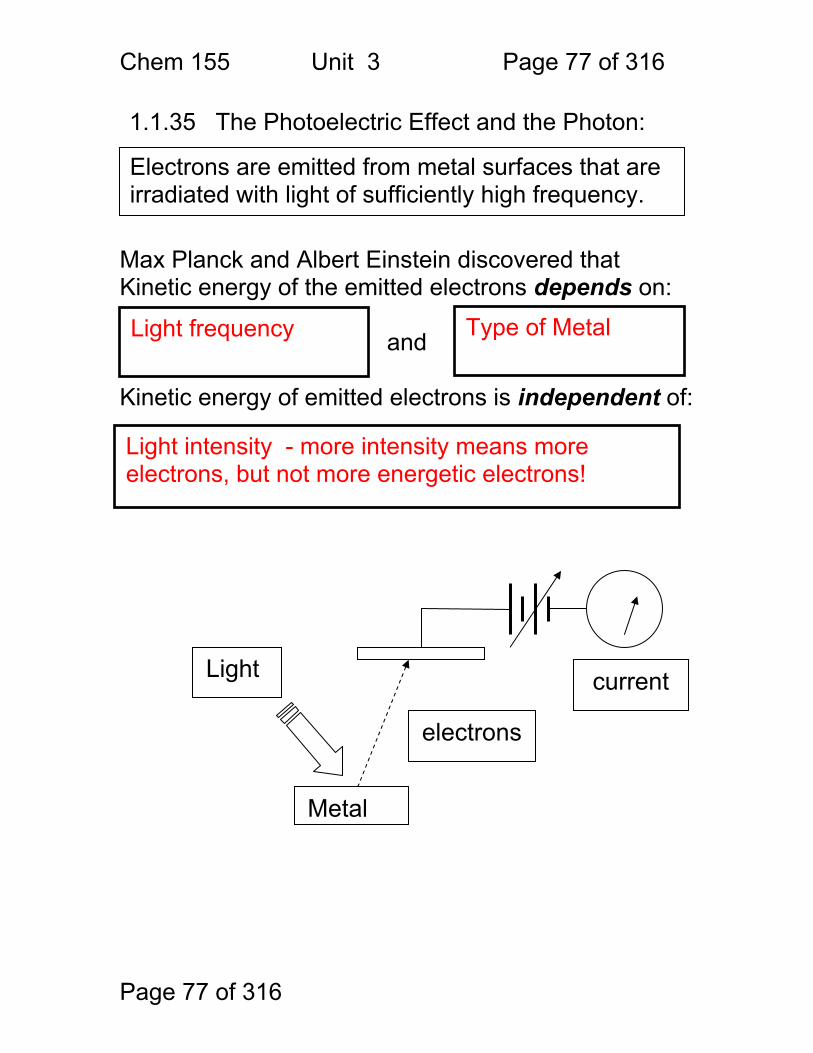
1.1.35 The Photoelectric Effect and the Photon: Max Planck and Albert Einstein discovered that Kinetic energy of the emitted electrons depends on:
and Kinetic energy of emitted electrons is independent of:
Metal
Light
electrons
current
Electrons are emitted from metal surfaces that are irradiated with light of sufficiently high frequency.
Light frequency Type of Metal
Light intensity - more intensity means more electrons, but not more energetic electrons!
Chem 155 Unit 3 Page 78 of 316
Page 78 of 316
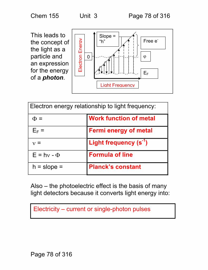
This leads to the concept of the light as a particle and an expression for the energy of a photon. Electron energy relationship to light frequency:
Φ = Work function of metal
EF = Fermi energy of metal
ν = Light frequency (s-1)
E = hν - Φ Formula of line
h = slope = Planck’s constant
Also – the photoelectric effect is the basis of many light detectors because it converts light energy into:
Light Frequency E
lect
ron
Ene
rgy
0 ϕ
EF
Free e- Slope = “h”
Electricity – current or single-photon pulses
Chem 155 Unit 3 Page 79 of 316
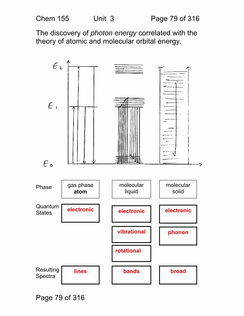
Page 79 of 316
The discovery of photon energy correlated with the theory of atomic and molecular orbital energy. Phase Quantum States Resulting Spectra
gas phase atom
molecular liquid
molecular solid
electronic electronic
lines
vibrational
broad
bands
rotational
electronic
phonon
Chem 155 Unit 3 Page 80 of 316
Page 80 of 316
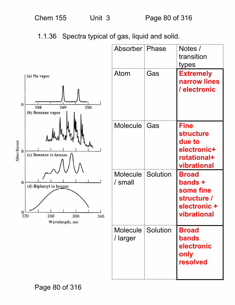
1.1.36 Spectra typical of gas, liquid and solid.
Absorber Phase Notes / transition types
Atom Gas Extremely narrow lines / electronic
Molecule Gas Fine structure due to electronic+ rotational+ vibrational
Molecule / small
Solution Broad bands + some fine structure / electronic + vibrational
Molecule / larger
Solution Broad bands electronic only resolved

Chem 155 Unit 3 Page 81 of 316
Page 81 of 316
1.1.37 Energy levels photon absorption emission.
Chem 155 Unit 3 Page 82 of 316
Page 82 of 316
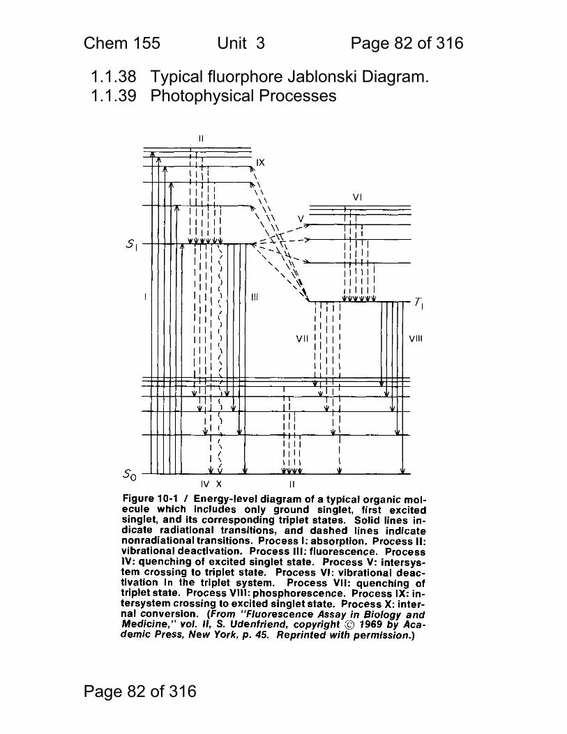
1.1.38 Typical fluorphore Jablonski Diagram. 1.1.39 Photophysical Processes
Chem 155 Unit 3 Page 83 of 316
Page 83 of 316
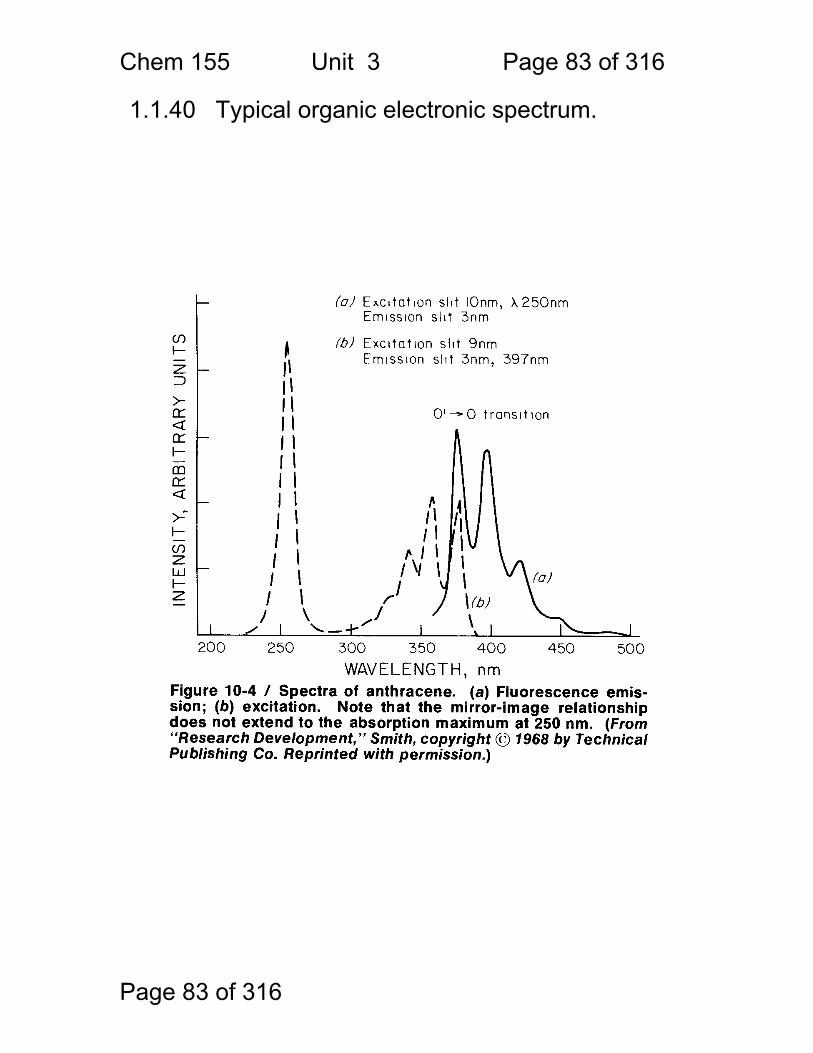
1.1.40 Typical organic electronic spectrum.
Chem 155 Unit 3 Page 84 of 316
Page 84 of 316
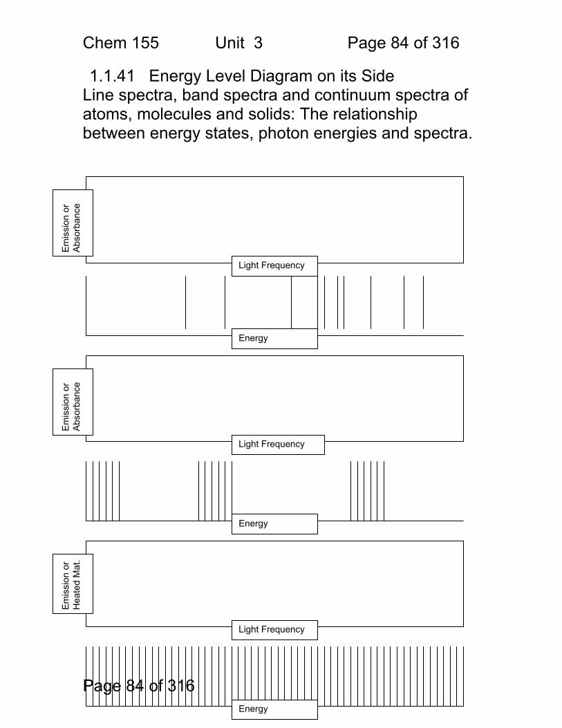
1.1.41 Energy Level Diagram on its Side Line spectra, band spectra and continuum spectra of atoms, molecules and solids: The relationship between energy states, photon energies and spectra.
Light Frequency
Light Frequency
Light Frequency
Em
issi
on o
r H
eate
d M
at.
Em
issi
on o
r A
bsor
banc
e E
mis
sion
or
Abs
orba
nce
Energy
Energy
Energy
Chem 155 Unit 3 Page 85 of 316
Page 85 of 316
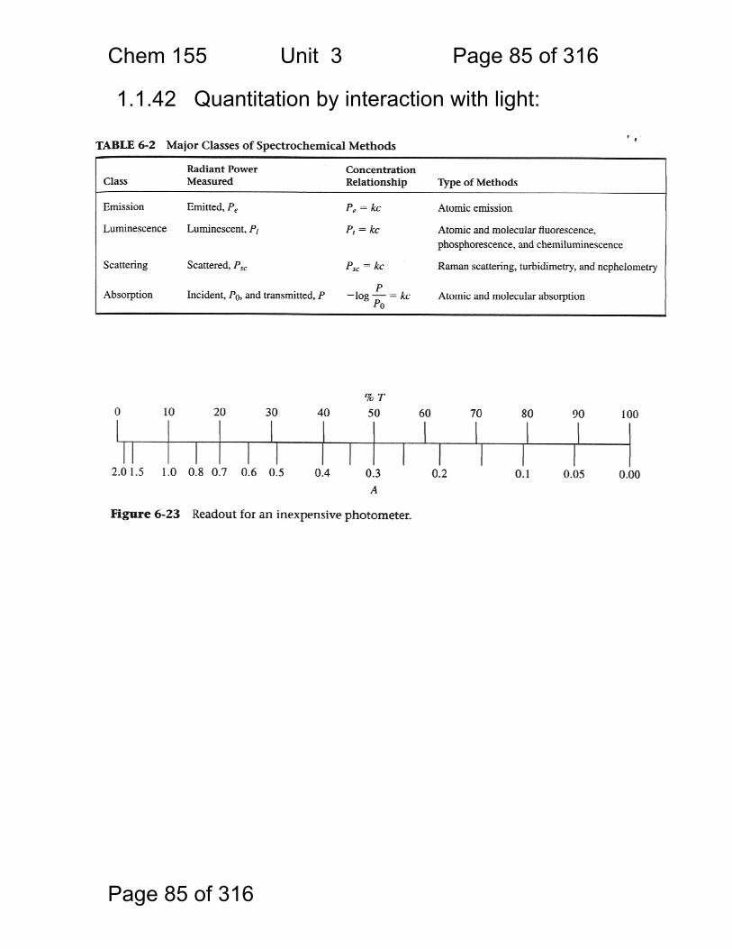
1.1.42 Quantitation by interaction with light:
Chem. 155 Unit 4 Page 86 of 316
Page 86 of 316
Photometric Methods and Spectroscopic Instrumentation
Skoog Chapters Covered: Review: Quantitation in Absorbance and Emission 7A Optical Designs – Absorbance Emission 7A Optical Materials (lightly!) 7B Light Sources Continuum and Line 7B Lasers!
Chem. 155 Unit 4 Page 87 of 316
Page 87 of 316
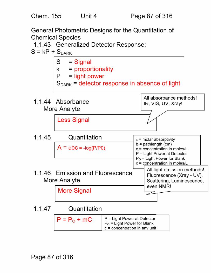
General Photometric Designs for the Quantitation of Chemical Species 1.1.43 Generalized Detector Response:
S = kP + SDARK 1.1.44 Absorbance
More Analyte 1.1.45 Quantitation
1.1.46 Emission and Fluorescence
More Analyte 1.1.47 Quantitation
Less Signal
A = εbc = -log(P/P0)
More Signal
P = PO + mC
ε = molar absorptivity b = pathlength (cm) c = concentration in moles/L P = Light Power at Detector PO = Light Power for Blank c = concentration in moles/L
P = Light Power at Detector PO = Light Power for Blank c = concentration in any unit
S = Signal k = proportionality P = light power SDARK = detector response in absence of light
All absorbance methods! IR, VIS, UV, Xray!
All light emission methods! Fluorescence (Xray - UV), Scattering, Luminescence, even NMR!
Chem. 155 Unit 4 Page 88 of 316
Page 88 of 316
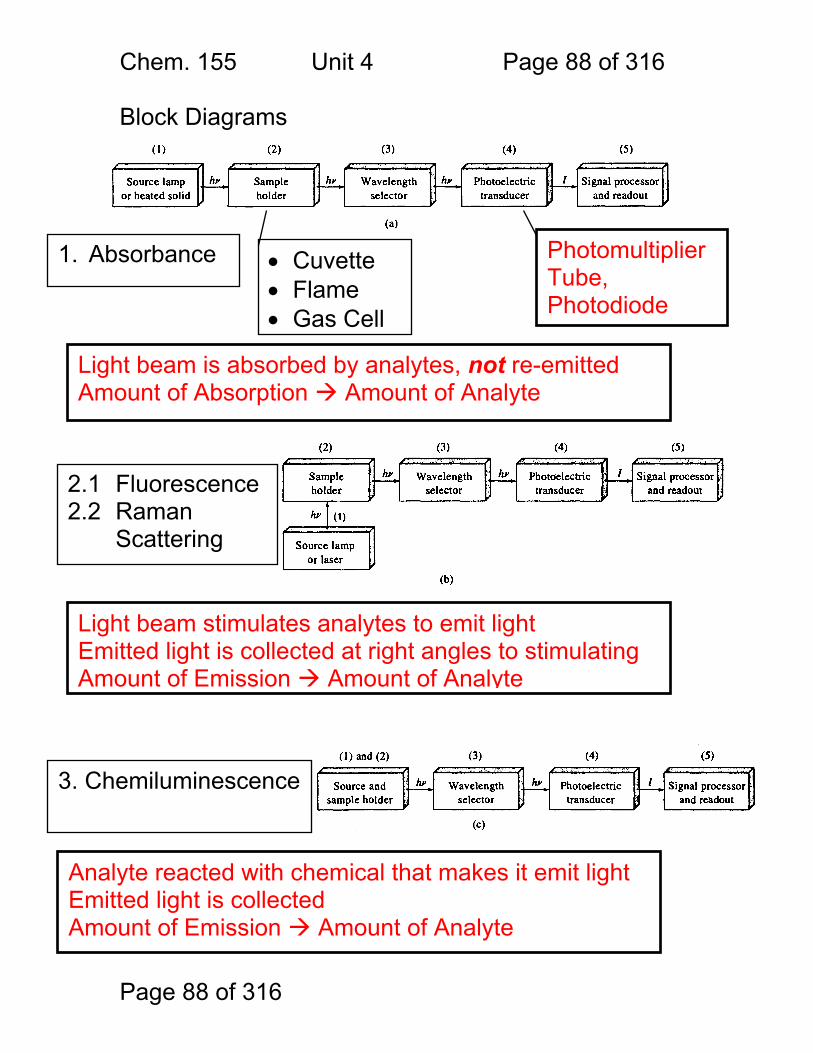
Block Diagrams Instruments for Analytical Spectrometry:
1. Absorbance • Cuvette • Flame • Gas Cell
2.1 Fluorescence 2.2 Raman
Scattering
3. Chemiluminescence
Light beam stimulates analytes to emit light Emitted light is collected at right angles to stimulating Amount of Emission Amount of Analyte
Photomultiplier Tube, Photodiode
Light beam is absorbed by analytes, not re-emitted Amount of Absorption Amount of Analyte
Analyte reacted with chemical that makes it emit light Emitted light is collected Amount of Emission Amount of Analyte
Chem. 155 Unit 4 Page 89 of 316
Page 89 of 316
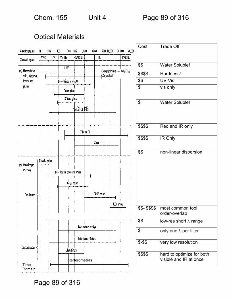
Optical Materials Cost Trade Off
$$ Water Soluble!
$$$$ Hardness! $$ UV-Vis $ vis only
$ Water Soluble!
$$$$ Red and IR only
$$$$ IR Only
$$ non-linear dispersion
$$- $$$$ most common tool order-overlap
$$ low-res short λ range
$ only one λ per filter
$-$$ very low resolution
$$$$ hard to optimize for both visible and IR at once Interferometers
LiF Sapphire – Al2O3 Crystal
Time Domain
Chem. 155 Unit 4 Page 90 of 316
Page 90 of 316
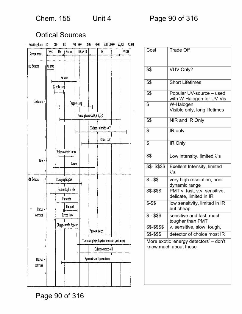
Optical Sources
Cost Trade Off
$$ VUV Only?
$$ Short Lifetimes
$$ Popular UV-source – used with W-Halogen for UV-Vis
$ W-Halogen Visible only, long lifetimes
$$ NIR and IR Only
$ IR only
$ IR Only
$$ Low intensity, limited λ’s
$$- $$$$ Exellent Intensity, limited λ’s
$ - $$ very high resolution, poor dynamic range
$$-$$$ PMT v. fast, v.v. sensitive, delicate, limited in IR
$-$$ low sensitvity, limited in IR but cheap
$ - $$$ sensitive and fast, much tougher than PMT
$$-$$$$ v. sensitive, slow, tough, $$-$$$ detector of choice most IR More exotic ‘energy detectors’ – don’t know much about these
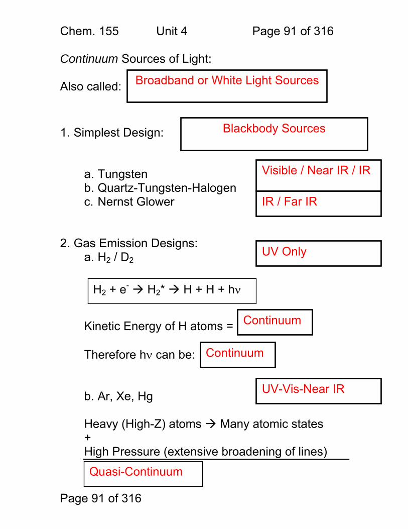
Chem. 155 Unit 4 Page 91 of 316
Page 91 of 316
Continuum Sources of Light: Also called: 1. Simplest Design:
a. Tungsten b. Quartz-Tungsten-Halogen c. Nernst Glower
2. Gas Emission Designs:
a. H2 / D2 Kinetic Energy of H atoms = Therefore hν can be: b. Ar, Xe, Hg Heavy (High-Z) atoms Many atomic states + High Pressure (extensive broadening of lines)
Broadband or White Light Sources
Blackbody Sources
Visible / Near IR / IR
IR / Far IR
H2 + e- H2* H + H + hν
Continuum
Continuum
Quasi-Continuum
UV-Vis-Near IR
UV Only
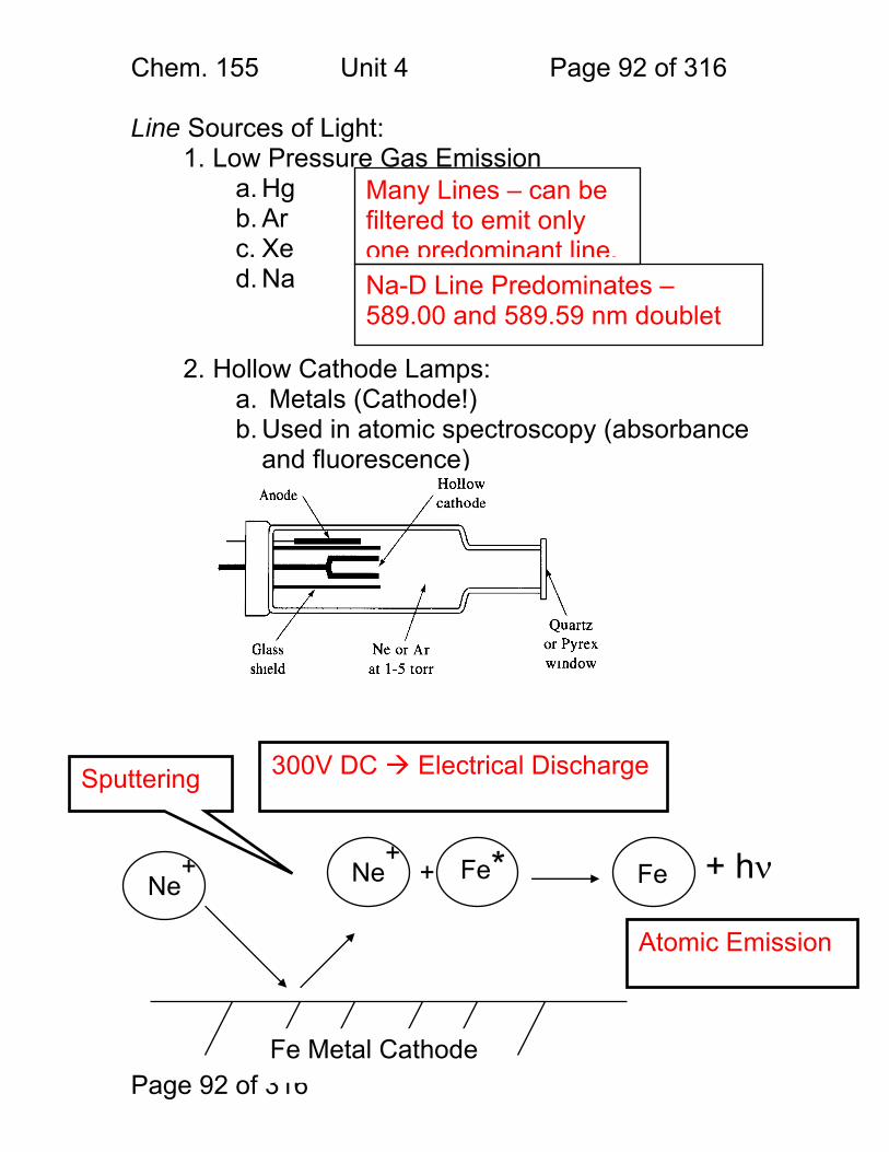
Chem. 155 Unit 4 Page 92 of 316
Page 92 of 316
Line Sources of Light: 1. Low Pressure Gas Emission
a. Hg b. Ar c. Xe d. Na
2. Hollow Cathode Lamps: a. Metals (Cathode!) b. Used in atomic spectroscopy (absorbance
and fluorescence)
Many Lines – can be filtered to emit only one predominant line.Na-D Line Predominates – 589.00 and 589.59 nm doublet
300V DC Electrical Discharge
Ne+
Ne+
Fe Metal Cathode
Fe* + Fe + hν
Sputtering
Atomic Emission
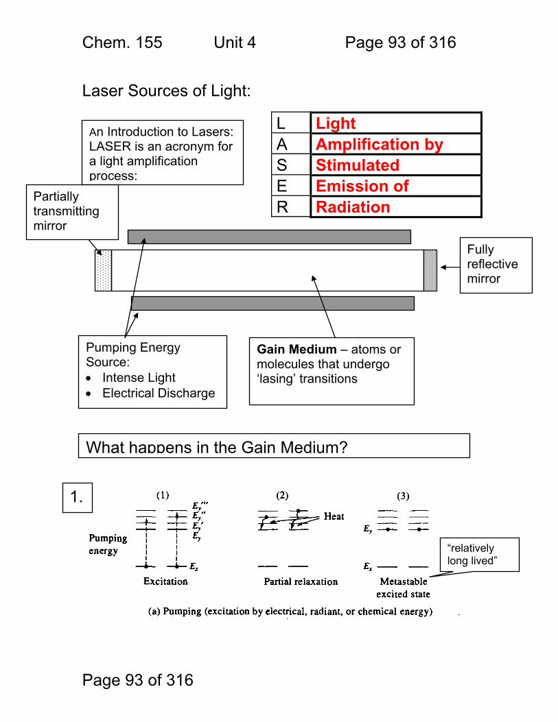
Chem. 155 Unit 4 Page 93 of 316
Page 93 of 316
Laser Sources of Light:
L Light A Amplification by S Stimulated E Emission of R Radiation
Pumping Energy Source: • Intense Light • Electrical Discharge
Partially transmitting mirror
Fully reflective mirror
Gain Medium – atoms or molecules that undergo ‘lasing’ transitions
What happens in the Gain Medium?
1.
“relatively long lived”
An Introduction to Lasers: LASER is an acronym for a light amplification process:
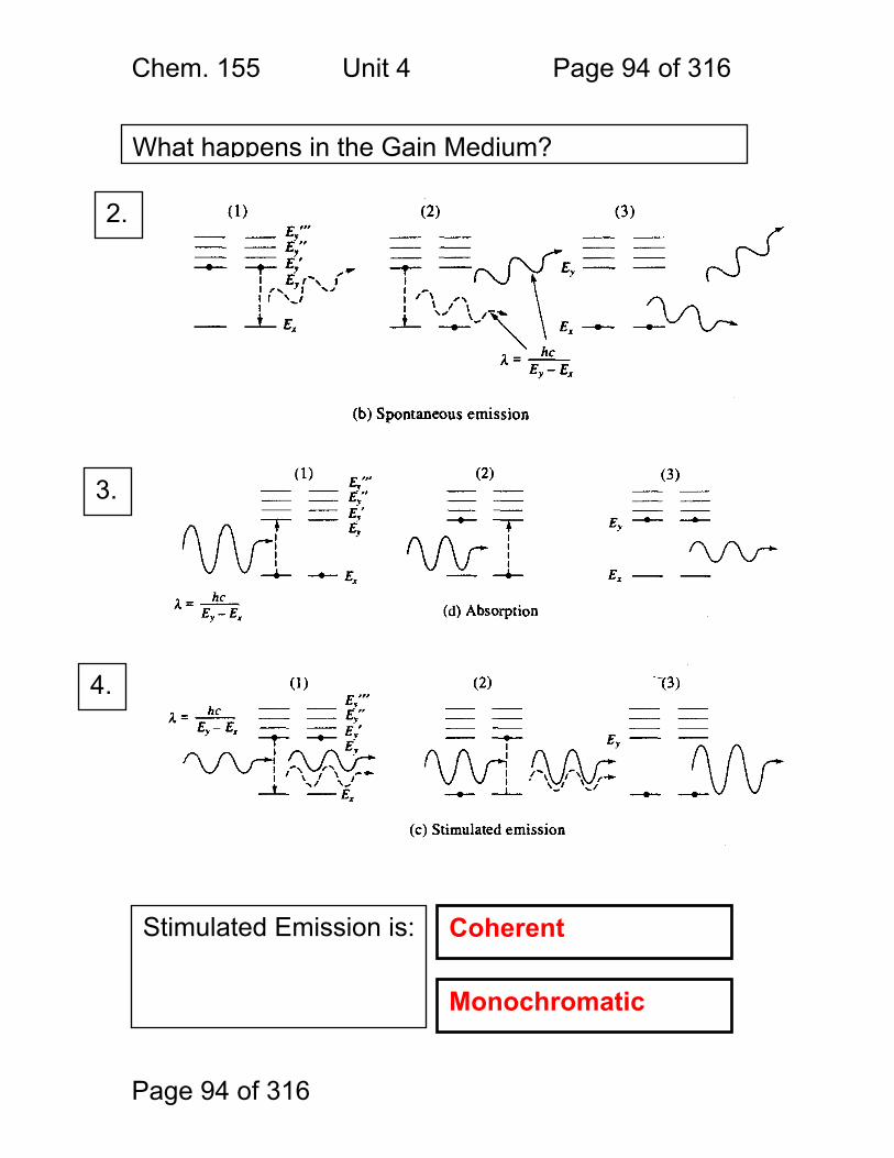
Chem. 155 Unit 4 Page 94 of 316
Page 94 of 316
What happens in the Gain Medium?
2.
3.
4.
Stimulated Emission is: Coherent
Monochromatic
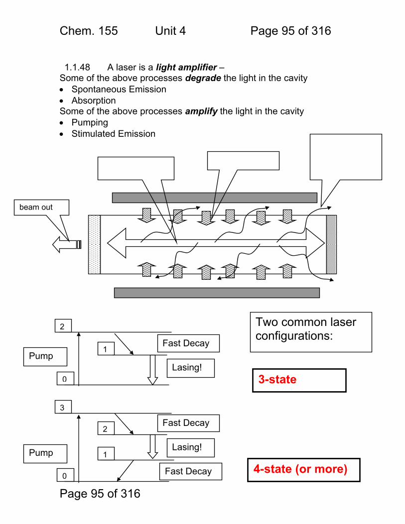
Chem. 155 Unit 4 Page 95 of 316
Page 95 of 316
1.1.48 A laser is a light amplifier –
Some of the above processes degrade the light in the cavity • Spontaneous Emission • Absorption Some of the above processes amplify the light in the cavity • Pumping • Stimulated Emission
Pump Fast Decay
Lasing!
beam out
0
1
2
Pump
Fast Decay
Lasing!
0
2
3
Fast Decay
1
Two common laser configurations:
3-state
4-state (or more)
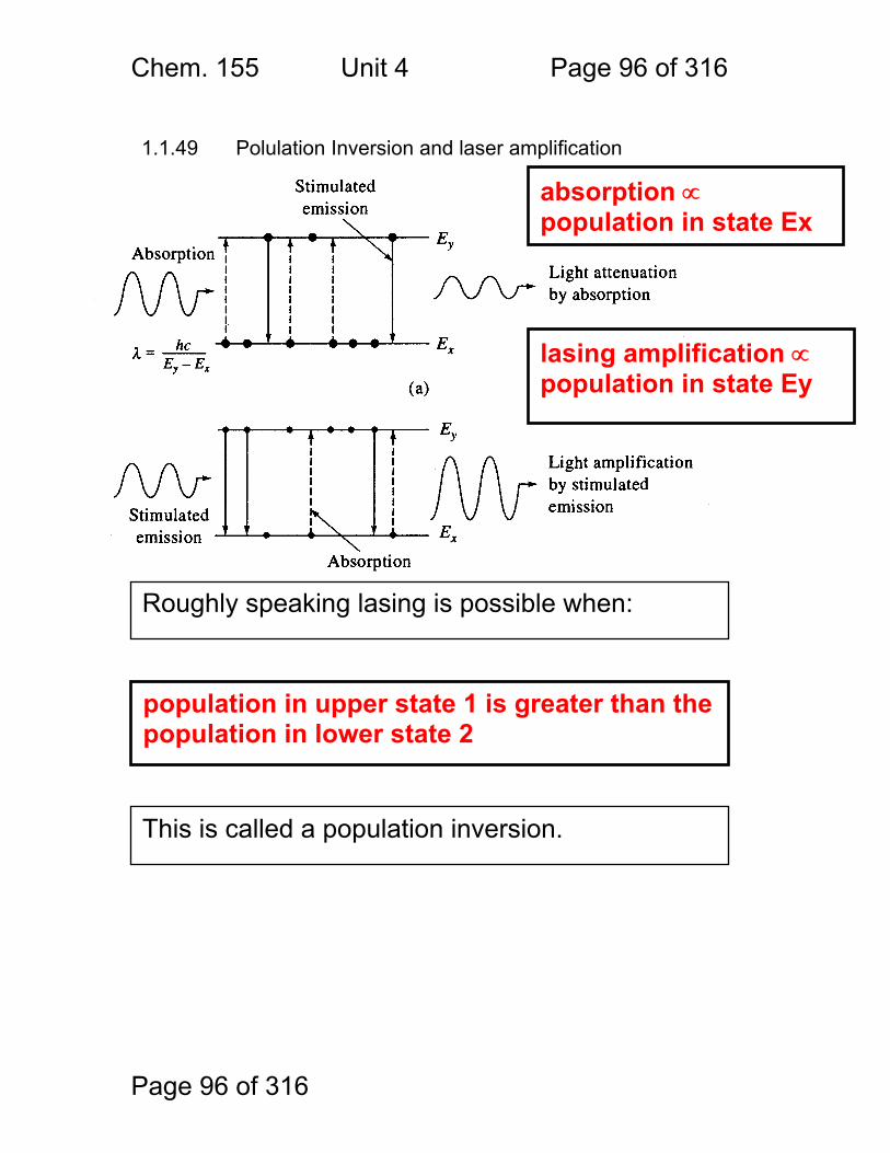
Chem. 155 Unit 4 Page 96 of 316
Page 96 of 316
1.1.49 Polulation Inversion and laser amplification
Roughly speaking lasing is possible when:
lasing amplification ∝ population in state Ey
absorption ∝ population in state Ex
population in upper state 1 is greater than the population in lower state 2
This is called a population inversion.

Chem. 155 Unit 4 Page 97 of 316
Page 97 of 316
1.1.50 Necessity of 3 or more states
Why are three or more levels (states) necessary for lasing?
N EXCITEDN GROUND
e
ΔEkTrecall:
ΔE = k = T = NEXCITED = NGROUND =
What happens when T infinity? NEXCITED NGROUND
Chem. 155 Unit 4 Page 98 of 316
Page 98 of 316
1.1.51 Common lasers categorized by lasing medium.
1. Solid Red - Near Infrared
1.1. Lanthanide-and transition metal ion lasers 1.1.1. Nd-YAG – Neodymium ions in a crystal called a ‘garnet’
made of yttrium oxide and aluminum oxide. Other lanthanide ions are substituted for other wavelengths in the near IR
1.1.2. Ho-ZBLA – Holmium (Ho+3) doped glasses made from ZrF3, BaF3, La F3, Al F3 can be fabricated into optical fibers that lase and can amplify optical signals of certain wavelengths
1.2. Semiconductor Lasers –
1.2.1. Silicon, 1.2.2. gallium arsenide and other light-emitting diodes can be
made to lase when many electrons are promoted to excited states within microfabricated cavities in the semiconductor crystal
Blue (very new) – Near Infrared 2. Liquid dye-lasers (blue-red) are made from solutions of many
different fluorescent dye molecules. The dye molecules have multiple excited-states that can be induced to lase usually by pumping with other lasers
3. Gas-Phase lasers (UV-near infrared) are very common, and
typically pumped by electrical discharge. Examples include: 3.1. He-Ne lasers (633 nm) 3.2. Ar-ion, Kr-ion (514, 488, 325 nm) 3.3. N2 (337 nm) 3.4. CO2 (10,600nm and many other IR wavelengths) 3.5. XeF (351) and KrF (248) and ArF (193) excimer lasers.
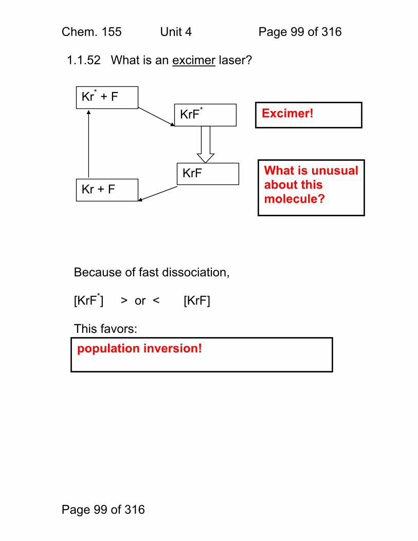
Chem. 155 Unit 4 Page 99 of 316
Page 99 of 316
1.1.52 What is an excimer laser? Because of fast dissociation, [KrF*] > or < [KrF] This favors:
Kr* + F
Kr + F
KrF*
KrF
Excimer!
What is unusual about this molecule?
population inversion!
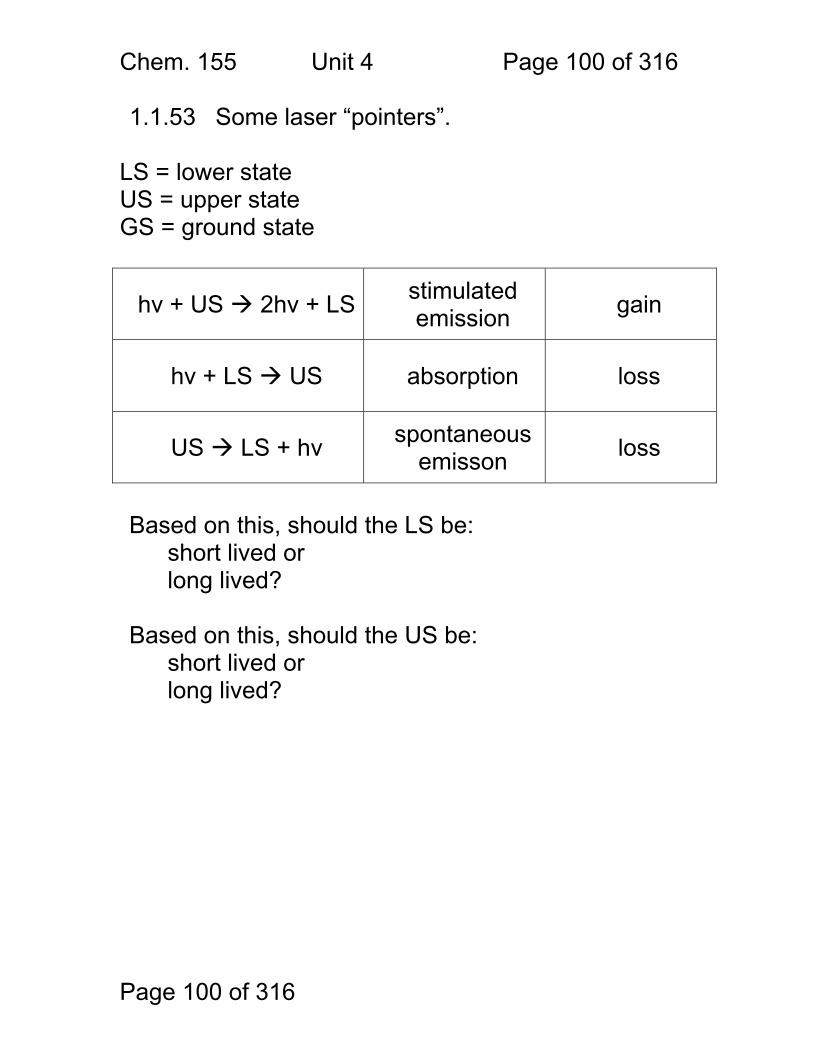
Chem. 155 Unit 4 Page 100 of 316
Page 100 of 316
1.1.53 Some laser “pointers”.
LS = lower state US = upper state GS = ground state
hν + US 2hν + LS stimulated emission gain
hν + LS US absorption loss
US LS + hν spontaneous emisson loss
Based on this, should the LS be:
short lived or long lived?
Based on this, should the US be: short lived or long lived?
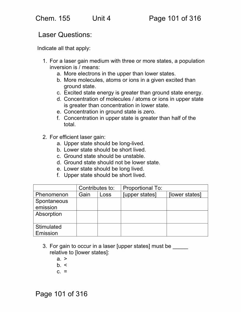
Chem. 155 Unit 4 Page 101 of 316
Page 101 of 316
Laser Questions: Indicate all that apply:
1. For a laser gain medium with three or more states, a population inversion is / means:
a. More electrons in the upper than lower states. b. More molecules, atoms or ions in a given excited than
ground state. c. Excited state energy is greater than ground state energy. d. Concentration of molecules / atoms or ions in upper state
is greater than concentration in lower state. e. Concentration in ground state is zero. f. Concentration in upper state is greater than half of the
total.
2. For efficient laser gain: a. Upper state should be long-lived. b. Lower state should be short lived. c. Ground state should be unstable. d. Ground state should not be lower state. e. Lower state should be long lived. f. Upper state should be short lived.
Contributes to: Proportional To: Phenomenon Gain Loss [upper states] [lower states] Spontaneous emission
Absorption
Stimulated Emission
3. For gain to occur in a laser [upper states] must be _____
relative to [lower states]: a. > b. < c. =
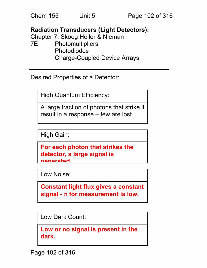
Chem 155 Unit 5 Page 102 of 316
Page 102 of 316
Radiation Transducers (Light Detectors): Chapter 7, Skoog Holler & Nieman 7E Photomultipliers Photodiodes Charge-Coupled Device Arrays Desired Properties of a Detector:
High Quantum Efficiency:
A large fraction of photons that strike it result in a response – few are lost.
High Gain:
For each photon that strikes the detector, a large signal is generated
Low Noise:
Constant light flux gives a constant signal - σ for measurement is low.
Low Dark Count:
Low or no signal is present in the dark.

Chem 155 Unit 5 Page 103 of 316
Page 103 of 316
Photoelectric effect photometers Phototube:
-+
Amplifier
Readout
Low work function metal: Na, K, GaAs
Photocathode – transducer - emits electrons via the photoelectric effect
High UV-transparency fused silica window.
Evacuated tube in which electrons can travel if emitted from cathode.
Anode – positive bias, collects photocurrent.
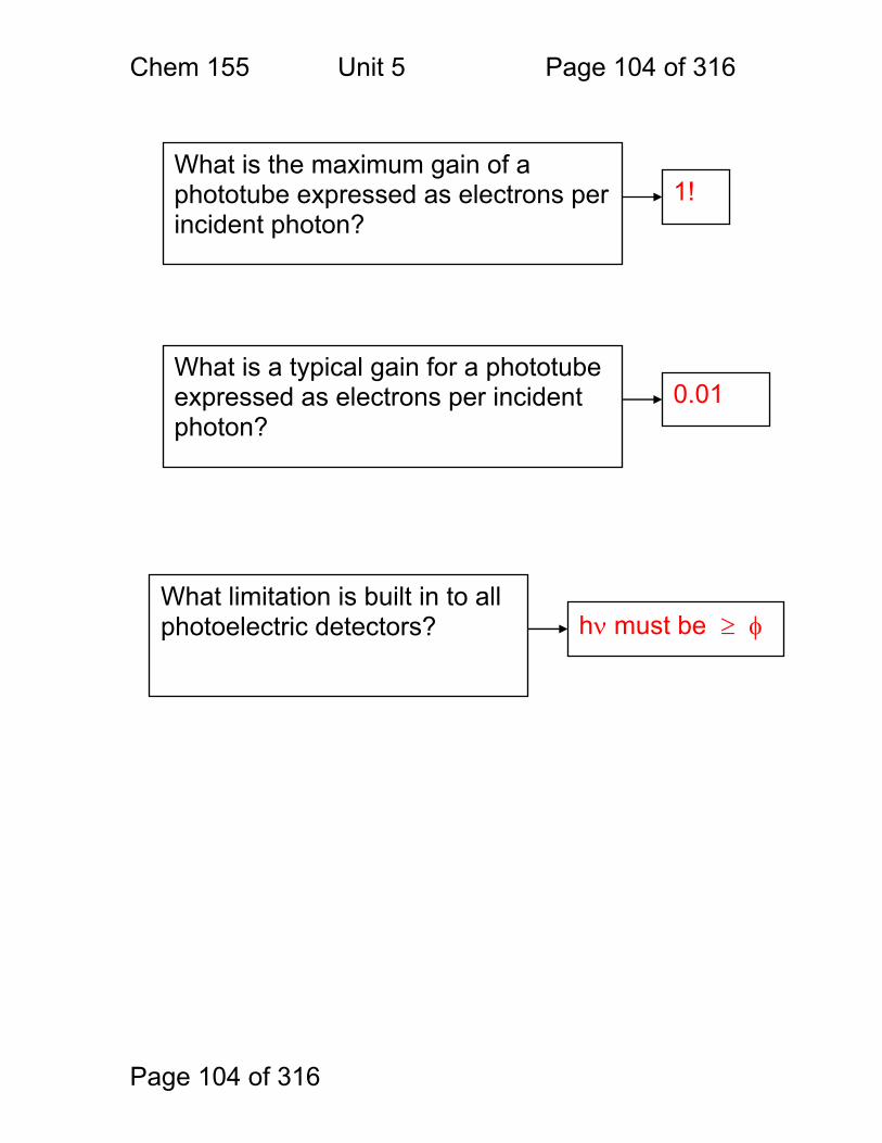
Chem 155 Unit 5 Page 104 of 316
Page 104 of 316
What is the maximum gain of a phototube expressed as electrons per incident photon?
1!
What is a typical gain for a phototube expressed as electrons per incident photon?
0.01
What limitation is built in to all photoelectric detectors? hν must be ≥ φ
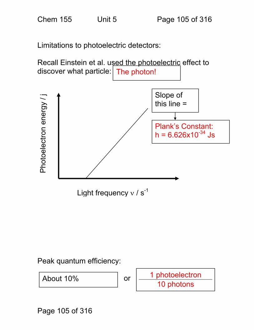
Chem 155 Unit 5 Page 105 of 316
Page 105 of 316
Limitations to photoelectric detectors: Recall Einstein et al. used the photoelectric effect to discover what particle: Peak quantum efficiency:
or
The photon!
About 10% 1 photoelectron 10 photons
Light frequency ν / s-1
Pho
toel
ectro
n en
ergy
/ j Slope of
this line =
Plank’s Constant: h = 6.626x10⁻³⁴ Js
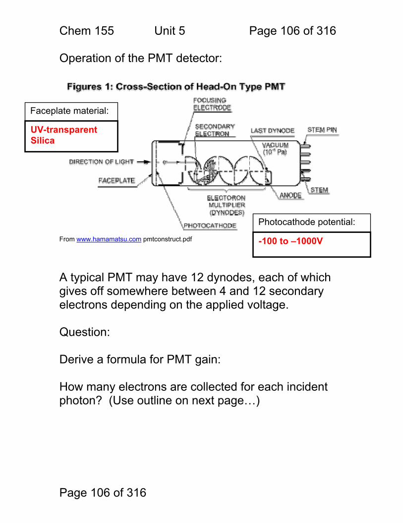
Chem 155 Unit 5 Page 106 of 316
Page 106 of 316
Operation of the PMT detector:
From www.hamamatsu.com pmtconstruct.pdf
A typical PMT may have 12 dynodes, each of which gives off somewhere between 4 and 12 secondary electrons depending on the applied voltage. Question: Derive a formula for PMT gain: How many electrons are collected for each incident photon? (Use outline on next page…)
Faceplate material:
UV-transparent Silica
Photocathode potential:
-100 to –1000V
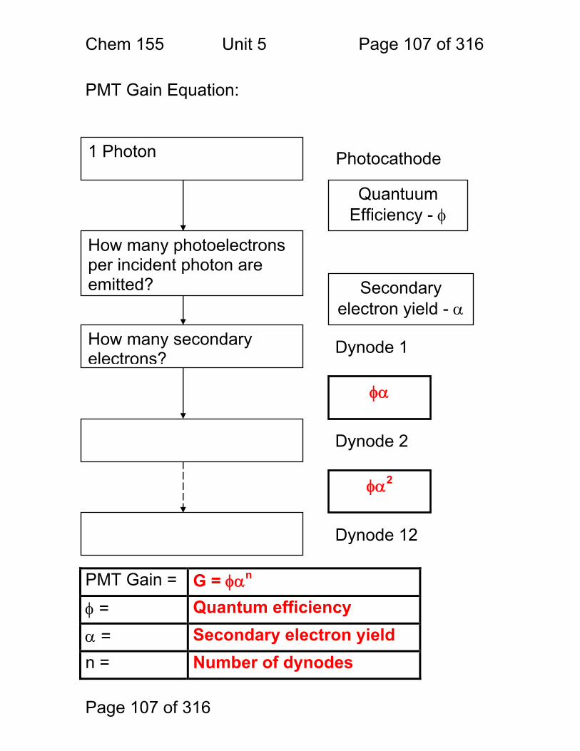
Chem 155 Unit 5 Page 107 of 316
Page 107 of 316
PMT Gain Equation:
PMT Gain = G = φαn φ = Quantum efficiency α = Secondary electron yield n = Number of dynodes
How many photoelectrons per incident photon are emitted? Secondary
electron yield - α
How many secondary electrons?
Dynode 1
1 Photon
Quantuum Efficiency - φ
φα
Dynode 2
φα2
Dynode 12
Photocathode
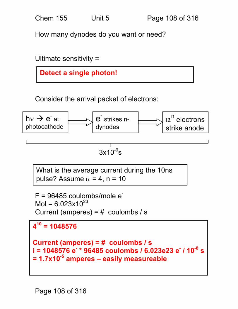
Chem 155 Unit 5 Page 108 of 316
Page 108 of 316
How many dynodes do you want or need? Ultimate sensitivity = Consider the arrival packet of electrons: F = 96485 coulombs/mole e- Mol = 6.023x10²³ Current (amperes) = # coulombs / s
Detect a single photon!
hν e- at photocathode
e- strikes n-dynodes
αn electrons strike anode
What is the average current during the 10ns pulse? Assume α = 4, n = 10
3x10⁻⁹s
410 = 1048576 Current (amperes) = # coulombs / s i = 1048576 e- * 96485 coulombs / 6.023e23 e- / 10-8 s = 1.7x10⁻⁵ amperes – easily measureable
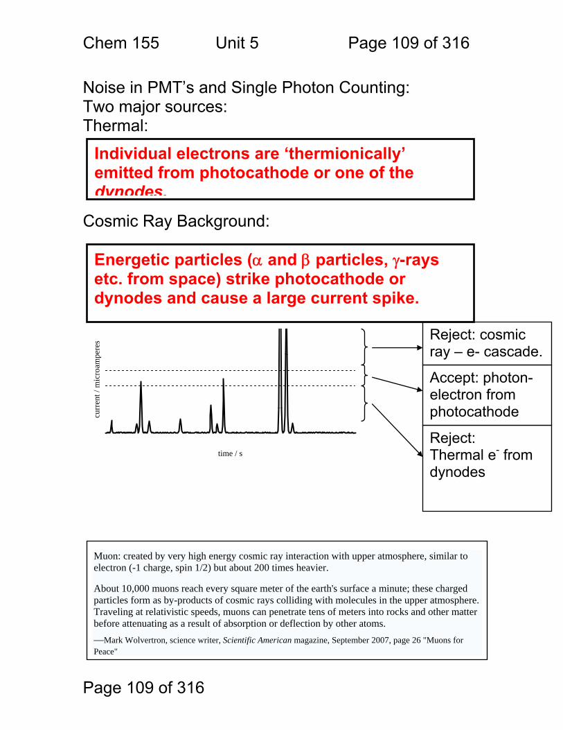
Chem 155 Unit 5 Page 109 of 316
Page 109 of 316
Noise in PMT’s and Single Photon Counting: Two major sources: Thermal: Cosmic Ray Background:
Individual electrons are ‘thermionically’ emitted from photocathode or one of the dynodes.
Energetic particles (α and β particles, γ-rays etc. from space) strike photocathode or dynodes and cause a large current spike.
Reject: Thermal e- from dynodes
Accept: photon-electron from photocathode
Reject: cosmic ray – e- cascade.
time / s
curr
ent /
mic
roam
pere
s
Muon: created by very high energy cosmic ray interaction with upper atmosphere, similar to electron (-1 charge, spin 1/2) but about 200 times heavier.
About 10,000 muons reach every square meter of the earth's surface a minute; these charged particles form as by-products of cosmic rays colliding with molecules in the upper atmosphere. Traveling at relativistic speeds, muons can penetrate tens of meters into rocks and other matter before attenuating as a result of absorption or deflection by other atoms. —Mark Wolvertron, science writer, Scientific American magazine, September 2007, page 26 "Muons for Peace"
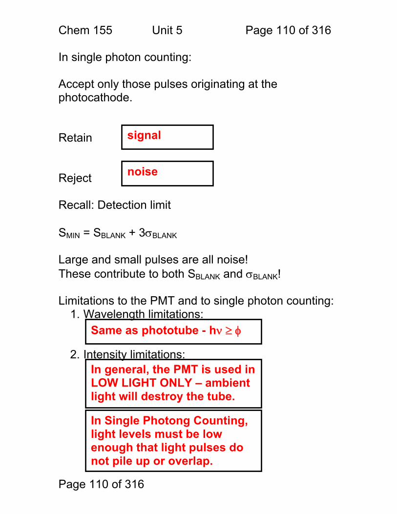
Chem 155 Unit 5 Page 110 of 316
Page 110 of 316
In single photon counting: Accept only those pulses originating at the photocathode. Retain Reject Recall: Detection limit SMIN = SBLANK + 3σBLANK Large and small pulses are all noise! These contribute to both SBLANK and σBLANK! Limitations to the PMT and to single photon counting:
1. Wavelength limitations:
2. Intensity limitations:
Same as phototube - hν ≥ φ
In general, the PMT is used in LOW LIGHT ONLY – ambient light will destroy the tube.
In Single Photong Counting, light levels must be low enough that light pulses do not pile up or overlap.
signal
noise
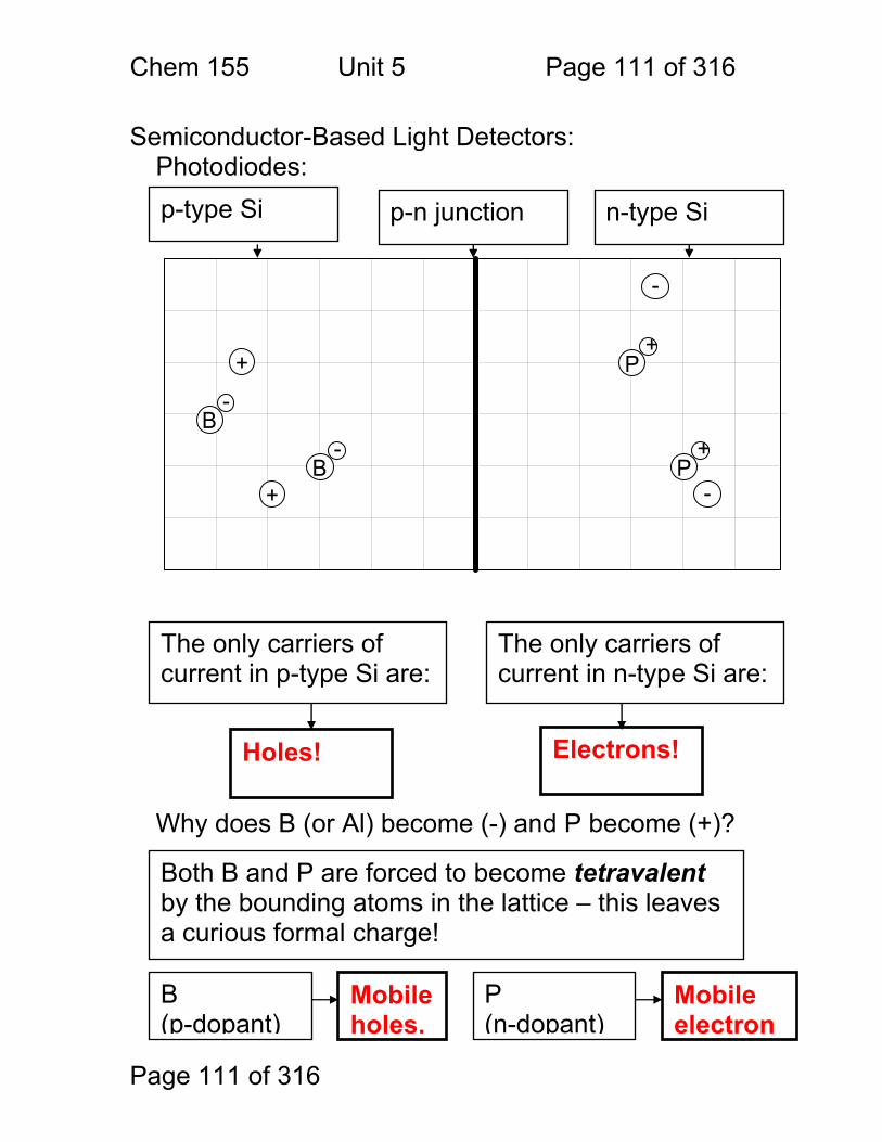
Chem 155 Unit 5 Page 111 of 316
Page 111 of 316
Semiconductor-Based Light Detectors: Photodiodes: Why does B (or Al) become (-) and P become (+)?
+
B-
B-
+P
+
-
P+
-
p-type Si n-type Si
The only carriers of current in p-type Si are:
The only carriers of current in n-type Si are:
Holes! Electrons!
Both B and P are forced to become tetravalent by the bounding atoms in the lattice – this leaves a curious formal charge!
B (p-dopant)
Mobile holes.
P (n-dopant)
Mobile electron
p-n junction
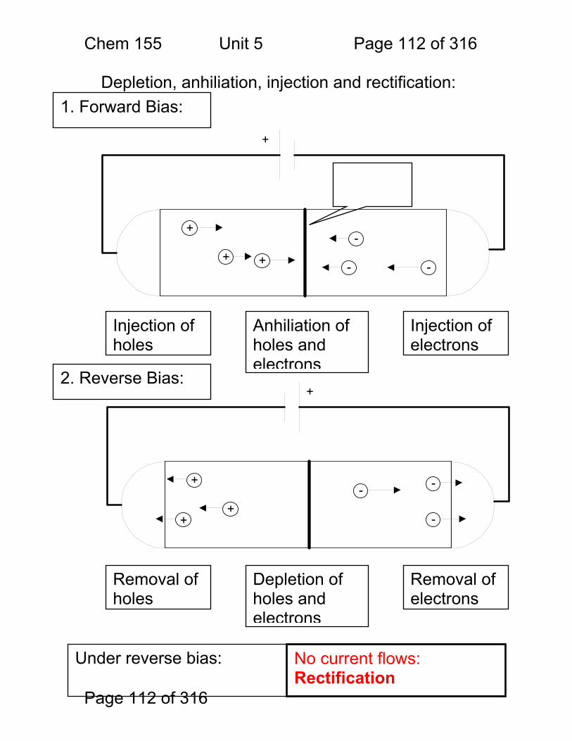
Chem 155 Unit 5 Page 112 of 316
Page 112 of 316
Depletion, anhiliation, injection and rectification:
+
+ +
-
- -
+
+
++
- -
-
+
Injection of holes
Anhiliation of holes and electrons
Injection of electrons
Removal of holes
Depletion of holes and electrons
Removal of electrons
1. Forward Bias:
2. Reverse Bias:
No current flows: Rectification
Under reverse bias:
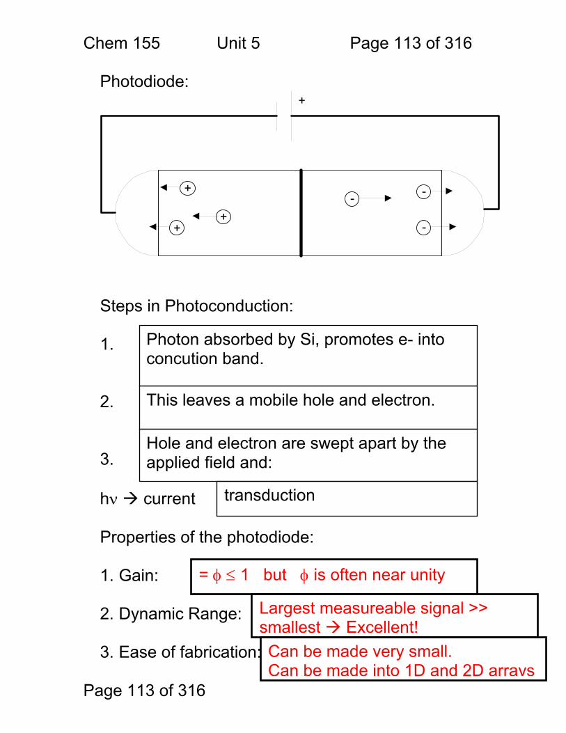
Chem 155 Unit 5 Page 113 of 316
Page 113 of 316
Photodiode:
+
++
- -
-
+
Steps in Photoconduction: 1. 2. 3. hν current Properties of the photodiode: 1. Gain:
2. Dynamic Range:
3. Ease of fabrication:
Photon absorbed by Si, promotes e- into concution band.
This leaves a mobile hole and electron.
Hole and electron are swept apart by the applied field and:
transduction
= φ ≤ 1 but φ is often near unity
Largest measureable signal >> smallest Excellent! Can be made very small. Can be made into 1D and 2D arrays
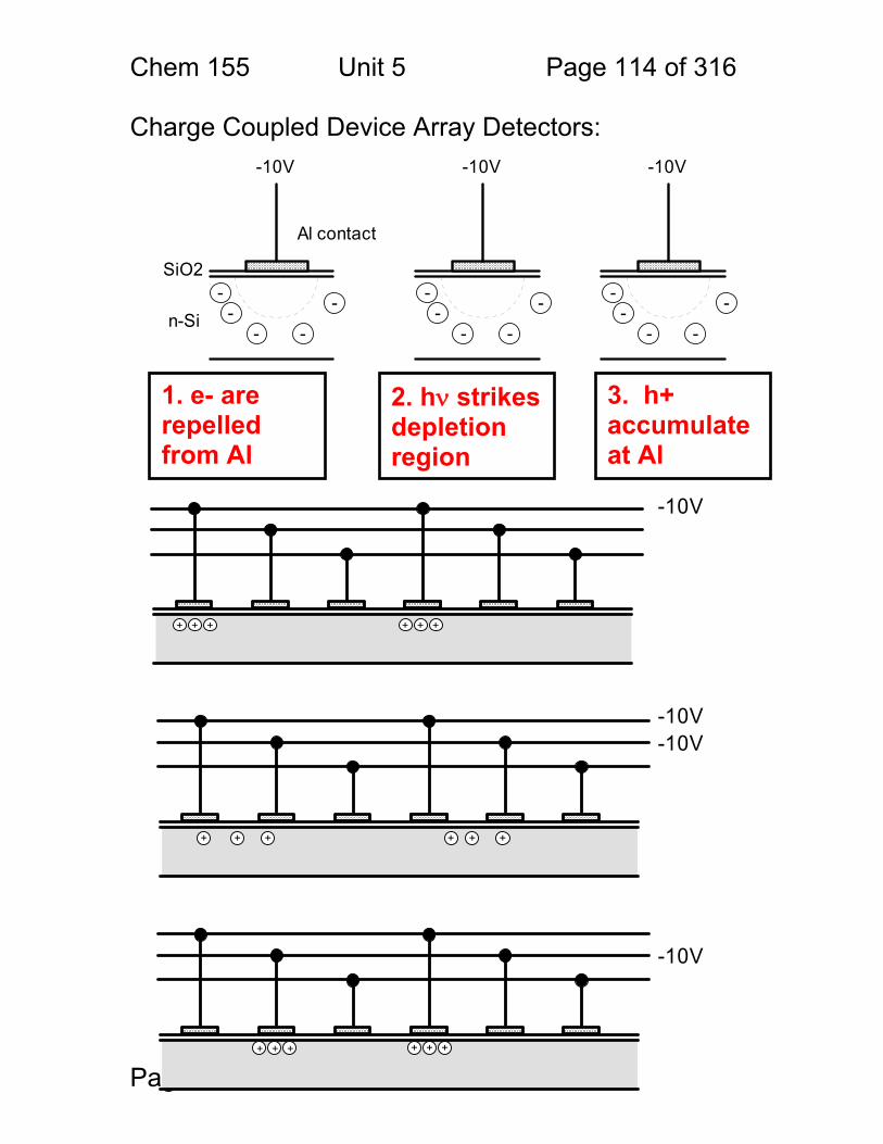
Chem 155 Unit 5 Page 114 of 316
Page 114 of 316
Charge Coupled Device Array Detectors:
1. e- are repelled from Al
2. hν strikes depletion region
3. h+ accumulate at Al
-10V
+ + +
+ + +
-10V
+ + + + +
-10V
+
-10V
+ + +
+ + +
-10V
Al contact
SiO2
n-Si -- -
--
-10V
-- -
--
-10V
-- -
--
Chem 155 Unit 5 Page 115 of 316
Page 115 of 316
CCD Array detectors are very useful for spectroscopy. 1. Maximum gain per pixel φ 1 2. Readout is relatively slow:
3. But, conventional spectrometers measure the
light spectrum (power versus wavelength) work by limiting the light incident on the detector to one wavelength at a time. With a CCD Array detector:
4. The light spectrum falls in a 2-dimensional image
or picture. 5. Thermal noise is lower than in PMT, but cannot
be completely rejected. 6. Cosmic ray background can be dealt with
statistically:
Not as sensitive as a PMT.
You can have a different detector for every wavelength CCD’s can acquire an entire spectrum much more quickly than a PMT-based system.
If there is a single particular pixel (spot on the picture) that is anomalously bright (i.e has an unusually high reading) – it can be rejected as cosmic radiation noise using statistical analysis.
Ca. 100 frames per second 10-2 s.
Chem 155 Unit 6 Page 116 of 316
Page 116 of 316
Monochromators for Atomic Spectroscopy: Chapter 7, Skoog Holler & Nieman 7C-2 Monochromators Dispersion Resolution Speed 7C-3 Monochromator Slits and Spectral Resolution Effective Bandwidth Line Convolution (Effect of Slit Width on Resolution) Czerny-Turner and Echelle designs Why do we care about monochromators? An analysis of the wavelength dependence of the absorbance or emission of light is called: This technique is used to: Measurement of the amount of monochromatic light absorbed or emitted by atoms or molecules is called: This technique can tell you:
analyze the structure of atoms and molecules
identify the atoms and molecules
Spectroscopy
observe interactions between atoms and molecules
Monochromatic light is useful!
Spectrometry
the concentration of atoms or molecules in a sample
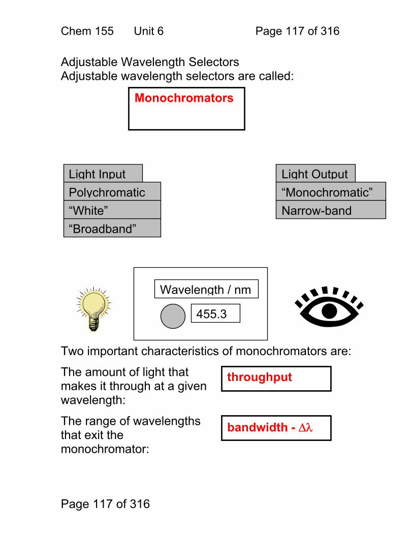
Chem 155 Unit 6 Page 117 of 316
Page 117 of 316
Adjustable Wavelength Selectors Adjustable wavelength selectors are called: Two important characteristics of monochromators are: The amount of light that makes it through at a given wavelength: The range of wavelengths that exit the monochromator:
Monochromators
Light Input Polychromatic “White” “Broadband”
Light Output“Monochromatic”Narrow-band
455.3
Wavelength / nm
throughput
bandwidth - Δλ
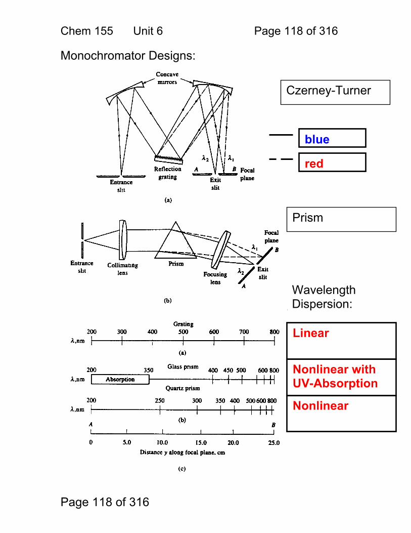
Chem 155 Unit 6 Page 118 of 316
Page 118 of 316
Monochromator Designs:
Czerney-Turner
Prism
Wavelength Dispersion:
Linear
Nonlinear with UV-Absorption
Nonlinear
blue
red
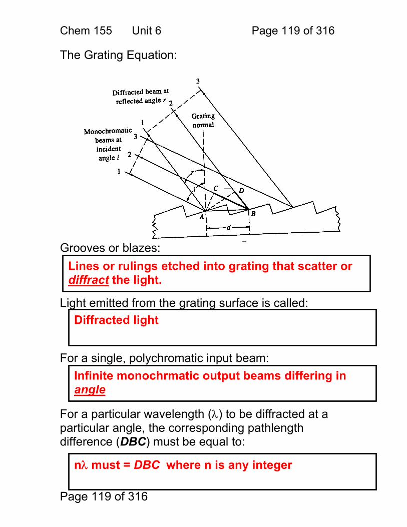
Chem 155 Unit 6 Page 119 of 316
Page 119 of 316
The Grating Equation: Grooves or blazes: Light emitted from the grating surface is called: For a single, polychromatic input beam: For a particular wavelength (λ) to be diffracted at a particular angle, the corresponding pathlength difference (DBC) must be equal to:
Lines or rulings etched into grating that scatter or diffract the light.
Diffracted light
Infinite monochrmatic output beams differing in angle
nλ must = DBC where n is any integer
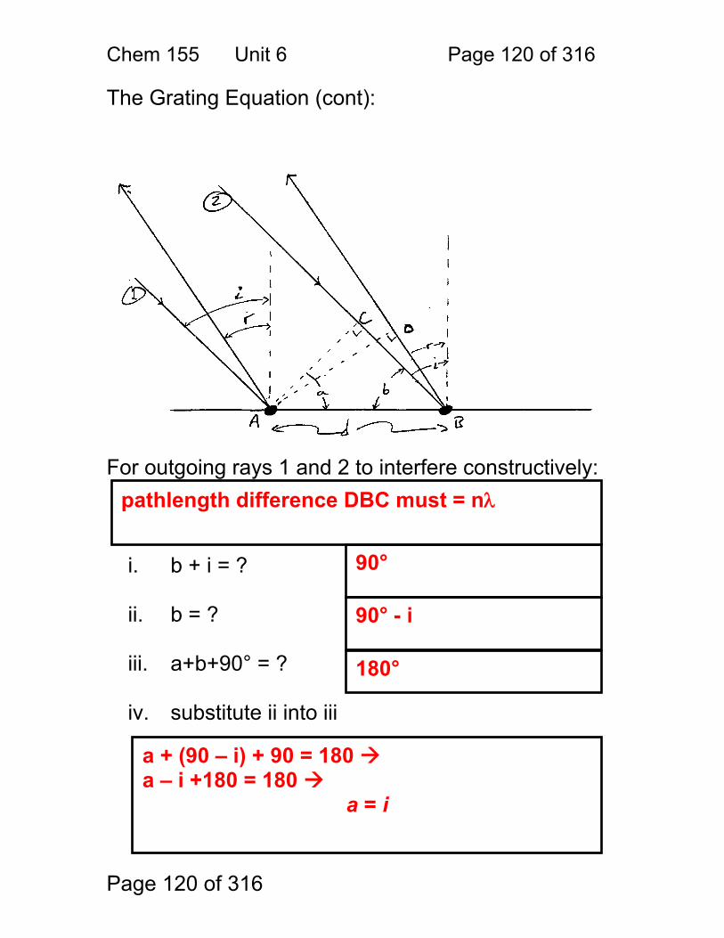
Chem 155 Unit 6 Page 120 of 316
Page 120 of 316
The Grating Equation (cont):
For outgoing rays 1 and 2 to interfere constructively:
i. b + i = ?
ii. b = ?
iii. a+b+90° = ?
iv. substitute ii into iii
pathlength difference DBC must = nλ
90°
90° - i
180°
a + (90 – i) + 90 = 180 a – i +180 = 180
a = i
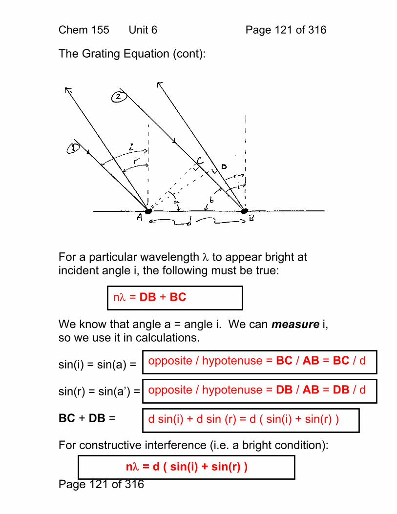
Chem 155 Unit 6 Page 121 of 316
Page 121 of 316
The Grating Equation (cont):
For a particular wavelength λ to appear bright at incident angle i, the following must be true: We know that angle a = angle i. We can measure i, so we use it in calculations. sin(i) = sin(a) = sin(r) = sin(a’) = BC + DB = For constructive interference (i.e. a bright condition):
nλ = DB + BC
opposite / hypotenuse = BC / AB = BC / d
opposite / hypotenuse = DB / AB = DB / d
d sin(i) + d sin (r) = d ( sin(i) + sin(r) )
nλ = d ( sin(i) + sin(r) )
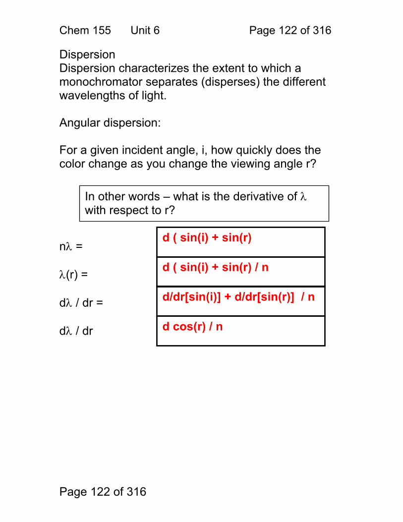
Chem 155 Unit 6 Page 122 of 316
Page 122 of 316
Dispersion Dispersion characterizes the extent to which a monochromator separates (disperses) the different wavelengths of light. Angular dispersion: For a given incident angle, i, how quickly does the color change as you change the viewing angle r? nλ = λ(r) = dλ / dr = dλ / dr
In other words – what is the derivative of λ with respect to r?
d ( sin(i) + sin(r)
d ( sin(i) + sin(r) / n
d/dr[sin(i)] + d/dr[sin(r)] / n
d cos(r) / n
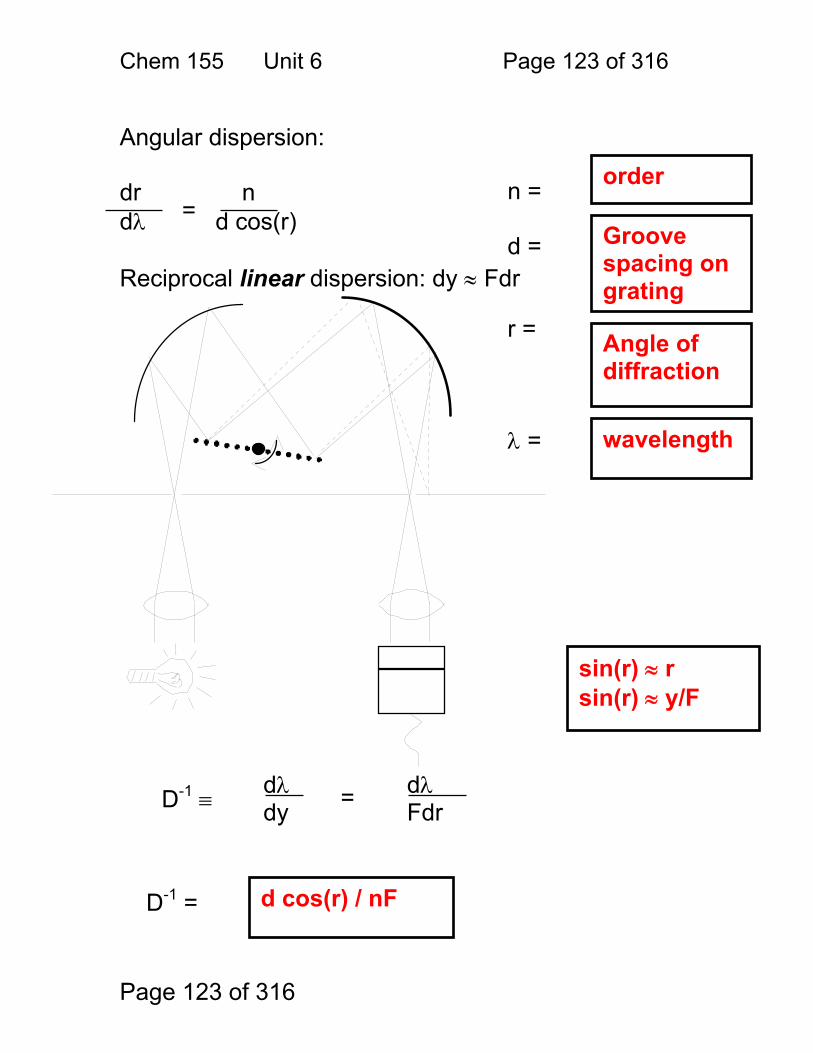
Chem 155 Unit 6 Page 123 of 316
Page 123 of 316
Angular dispersion: dr n dλ d cos(r) Reciprocal linear dispersion: dy ≈ Fdr
dλ dλ dy Fdr
=n = d = r = λ =
D-1 ≡ =
D-1 =
order
Groove spacing on grating
Angle of diffraction
wavelength
sin(r) ≈ r sin(r) ≈ y/F
d cos(r) / nF
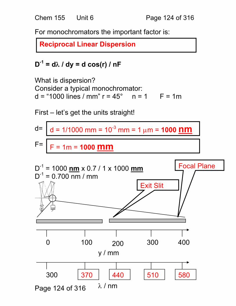
Chem 155 Unit 6 Page 124 of 316
Page 124 of 316
For monochromators the important factor is: D-1 = dλ / dy = d cos(r) / nF What is dispersion? Consider a typical monochromator: d = “1000 lines / mm” r = 45° n = 1 F = 1m First – let’s get the units straight! d= F= D-1 = 1000 nm x 0.7 / 1 x 1000 mm D-1 = 0.700 nm / mm
Reciprocal Linear Dispersion
Focal Plane
Exit Slit
y / mm0 100 200 300 400
λ / nm300 370 440 510 580
d = 1/1000 mm = 10-3 mm = 1 μm = 1000 nm
F = 1m = 1000 mm
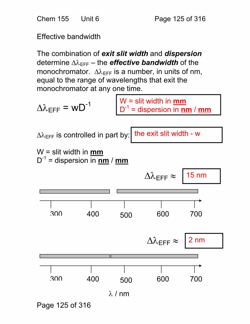
Chem 155 Unit 6 Page 125 of 316
Page 125 of 316
Effective bandwidth The combination of exit slit width and dispersion determine ΔλEFF – the effective bandwidth of the monochromator. ΔλEFF is a number, in units of nm, equal to the range of wavelengths that exit the monochromator at any one time. ΔλEFF = wD-1 ΔλEFF is controlled in part by: W = slit width in mm D-1 = dispersion in nm / mm
the exit slit width - w
300 400 500 600 700
ΔλEFF ≈ 15 nm
300 400 500 600 700
λ / nm
ΔλEFF ≈ 2 nm
W = slit width in mm D-1 = dispersion in nm / mm
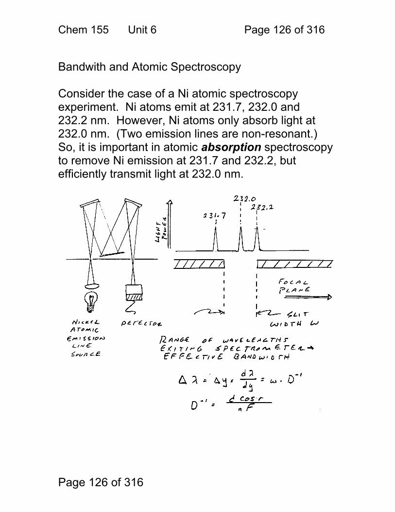
Chem 155 Unit 6 Page 126 of 316
Page 126 of 316
Bandwith and Atomic Spectroscopy Consider the case of a Ni atomic spectroscopy experiment. Ni atoms emit at 231.7, 232.0 and 232.2 nm. However, Ni atoms only absorb light at 232.0 nm. (Two emission lines are non-resonant.) So, it is important in atomic absorption spectroscopy to remove Ni emission at 231.7 and 232.2, but efficiently transmit light at 232.0 nm.
Chem 155 Unit 6 Page 127 of 316
Page 127 of 316
Factors That Control ΔλEFF In general, one wants a monochromator with as small an effective bandwidth is practical. Such a monochormator is called: To achieve low effective bandwith / high resolution ΔλEFF should be: ΔλEFF = wD-1 = wd cos(r) / nF , so d should be: F should be: w should be: The essential tradeoff is that very small ΔλEFF usually equate to low light levels. For example, achieving very small ΔλEFF by making w very small is often unsuccessful because the source is imaged onto the focal plane. Unless the source is a very bright, point source, then making w is smaller than the source will often cause light levels to drop dramatically.
small
large
high resolution
small
small
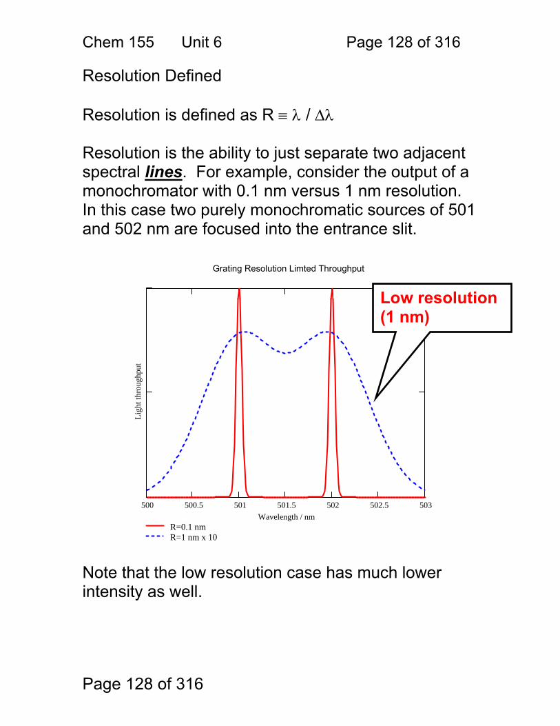
Chem 155 Unit 6 Page 128 of 316
Page 128 of 316
Resolution Defined Resolution is defined as R ≡ λ / Δλ Resolution is the ability to just separate two adjacent spectral lines. For example, consider the output of a monochromator with 0.1 nm versus 1 nm resolution. In this case two purely monochromatic sources of 501 and 502 nm are focused into the entrance slit.
Note that the low resolution case has much lower intensity as well.
Grating Resolution Limted Throughput
500 500.5 501 501.5 502 502.5 503
R=0.1 nmR=1 nm x 10
Wavelength / nm
Ligh
t thr
ough
put
Low resolution (1 nm)
Chem 155 Unit 6 Page 129 of 316
Page 129 of 316
Grating Resolution Resolution may be limited by the size of the grating as well. The grating resolution, R, is given by: R ≡ λ / Δλ = nN n = N = Grating resolution imposes a kind of effective bandwidth limitation Δλ just like the ΔλEFF defined above Please note these three things:
1. Both grating resolution and effective bandwith define a minimum resolvable Δλ for the monochromator.
2. A given monochromator will be limited by the worse of the two parameters.
3. This is usually ΔλEFF
Diffraction order
Number of grooves of the grating that are illuminated
Chem 155 Unit 6 Page 130 of 316
Page 130 of 316
Grating Resolution Exercise:
How large must a 1000 groove/mm grating be to give a resolution of 1nm at 500nm? (Assume that the monochromator is functioning in first order.)
R = λ / Δλ = nN N = n λ / Δλ = 1*500/0.1 = 5000 grooves 5000 grooves / 1000 grooves/mm = 5 mm!
Chem 155 Unit 6 Page 131 of 316
Page 131 of 316
If a Czerny-Turner monochromator has the following specifications:
Holographically-ruled diffraction grating with 1582 grooves per mm. 250 mm focal length Grating position such that the diffracted angle is 45 degrees Operation in first order A slit width of 0.5 mm
a. What is the reciprocal linear dispersion effective bandwidth of this
monochromator (use appropriate units)?
b. What is the effective bandwidth of this monochromator (use appropriate units)?
A Czerny-Turner monochromator is set to 300.00 nm and the slits are set so that the effective bandwidth is 1.0 nm. If a broadband UV light source is directed into the monochromator, what wavelengths of light will exit? What type of light source might be appropriate for this experiment? If a Czerny-Turner monochromator has the following specifications:
a. Holographically-ruled diffraction grating with 940 grooves per mm. b. 250 mm focal length c. Grating position such that the refracted angle is 45 degrees d. Operation in first order
What slit width is required to give this monochromator an effective bandwidth of 0.5 nm? How big must the grating be in order to achieve this resolution (R).
Chem 155 Unit 6 Page 132 of 316
Page 132 of 316
High Resolution and Echelle Monochromators Atomic spectroscopy demands high resolution because atomic absorption / emission lines are:
So we want effective bandwidth ΔλEFF = wD-1 = w d cos(r) / nF to be: We also want resolution (R = λ / Δλ = nN) to be: ΔλEFF R w should be small - d should be small small F should be large large n should be large large But there are limitations to the above: w d F What about n?
1. narrow 2.
small
large
n is the key…
If w is too small 1 – no light 2 – exceeds the ability to focus light
Limitations in the fabrication of gratings
How big of a spectrometer is tolerable?
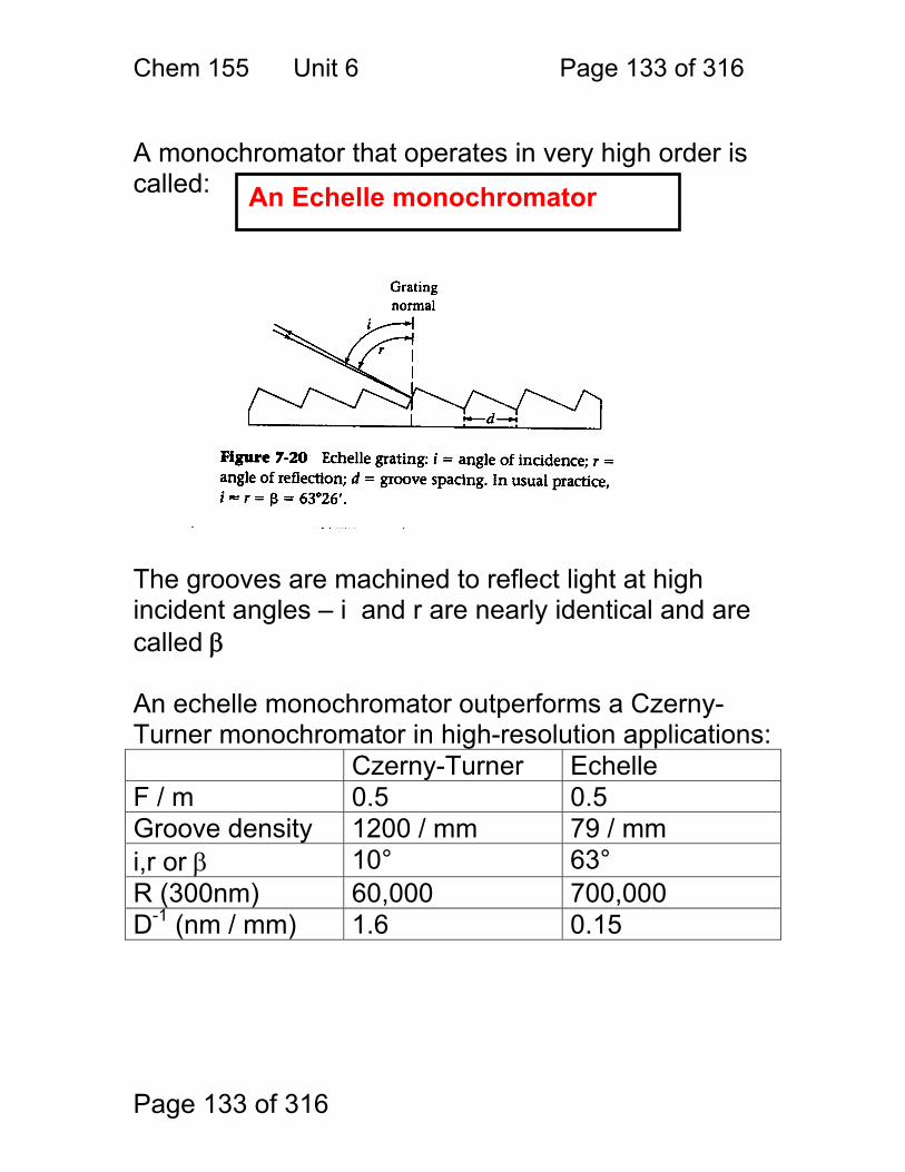
Chem 155 Unit 6 Page 133 of 316
Page 133 of 316
A monochromator that operates in very high order is called:
The grooves are machined to reflect light at high incident angles – i and r are nearly identical and are called β An echelle monochromator outperforms a Czerny-Turner monochromator in high-resolution applications: Czerny-Turner Echelle F / m 0.5 0.5 Groove density 1200 / mm 79 / mm i,r or β 10° 63° R (300nm) 60,000 700,000 D-1 (nm / mm) 1.6 0.15
An Echelle monochromator
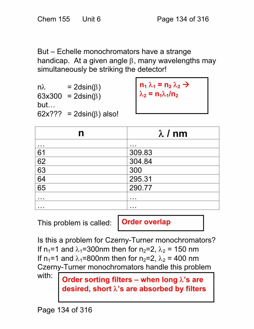
Chem 155 Unit 6 Page 134 of 316
Page 134 of 316
But – Echelle monochromators have a strange handicap. At a given angle β, many wavelengths may simultaneously be striking the detector! nλ = 2dsin(β) 63x300 = 2dsin(β) but… 62x??? = 2dsin(β) also!
n λ / nm
… … 61 309.83 62 304.84 63 300 64 295.31 65 290.77 … … … … This problem is called: Is this a problem for Czerny-Turner monochromators? If n1=1 and λ1=300nm then for n2=2, λ2 = 150 nm If n1=1 and λ1=800nm then for n2=2, λ2 = 400 nm Czerny-Turner monochromators handle this problem with:
n1 λ1 = n2 λ2 λ2 = n1λ1/n2
Order overlap
Order sorting filters – when long λ’s are desired, short λ’s are absorbed by filters
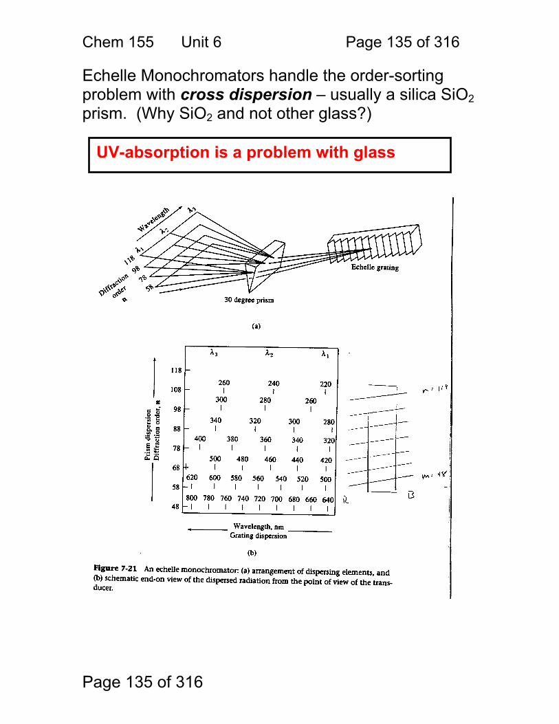
Chem 155 Unit 6 Page 135 of 316
Page 135 of 316
Echelle Monochromators handle the order-sorting problem with cross dispersion – usually a silica SiO2 prism. (Why SiO2 and not other glass?) UV-absorption is a problem with glass
Chem 155 Unit 6 Page 136 of 316
Page 136 of 316
This means that the Echelle monochromator has a 2-dimensional focal plane! What kind of detector is tailor-made for an Echelle mnochromator The CCD array detector!
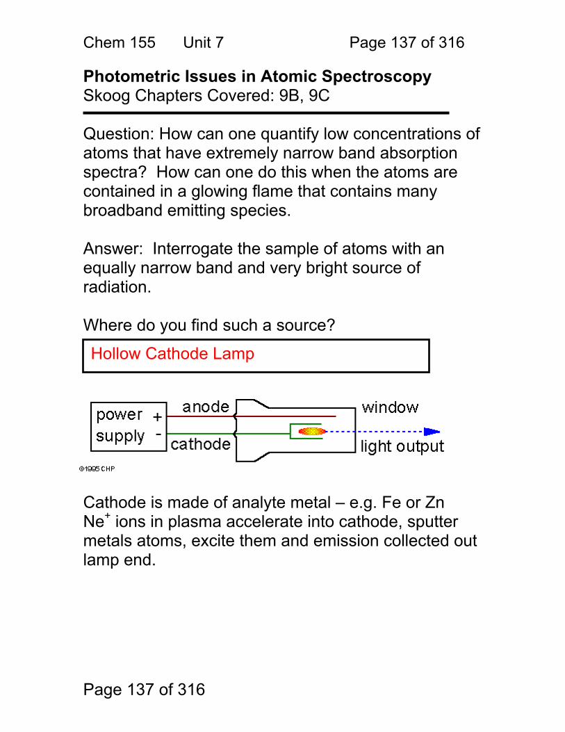
Chem 155 Unit 7 Page 137 of 316
Page 137 of 316
Photometric Issues in Atomic Spectroscopy Skoog Chapters Covered: 9B, 9C Question: How can one quantify low concentrations of atoms that have extremely narrow band absorption spectra? How can one do this when the atoms are contained in a glowing flame that contains many broadband emitting species. Answer: Interrogate the sample of atoms with an equally narrow band and very bright source of radiation. Where do you find such a source?
Cathode is made of analyte metal – e.g. Fe or Zn Ne+ ions in plasma accelerate into cathode, sputter metals atoms, excite them and emission collected out lamp end.
Hollow Cathode Lamp
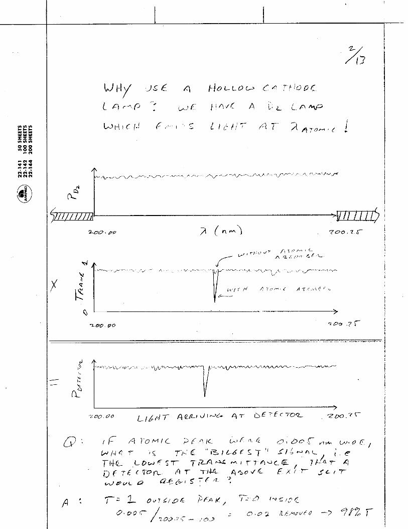
Chem 155 Unit 7 Page 138 of 316
Page 138 of 316
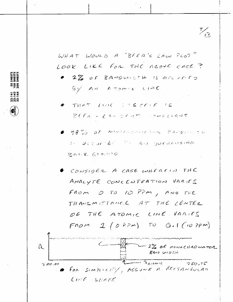
Chem 155 Unit 7 Page 139 of 316
Page 139 of 316
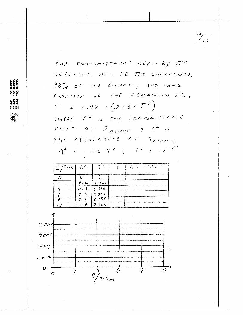
Chem 155 Unit 7 Page 140 of 316
Page 140 of 316
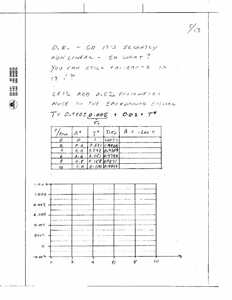
Chem 155 Unit 7 Page 141 of 316
Page 141 of 316

Chem 155 Unit 7 Page 142 of 316
Page 142 of 316
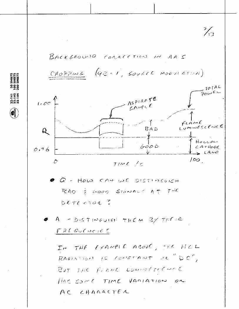
Chem 155 Unit 7 Page 143 of 316
Page 143 of 316
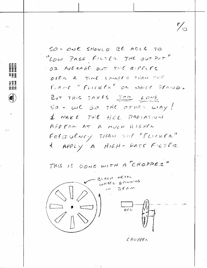
Chem 155 Unit 7 Page 144 of 316
Page 144 of 316
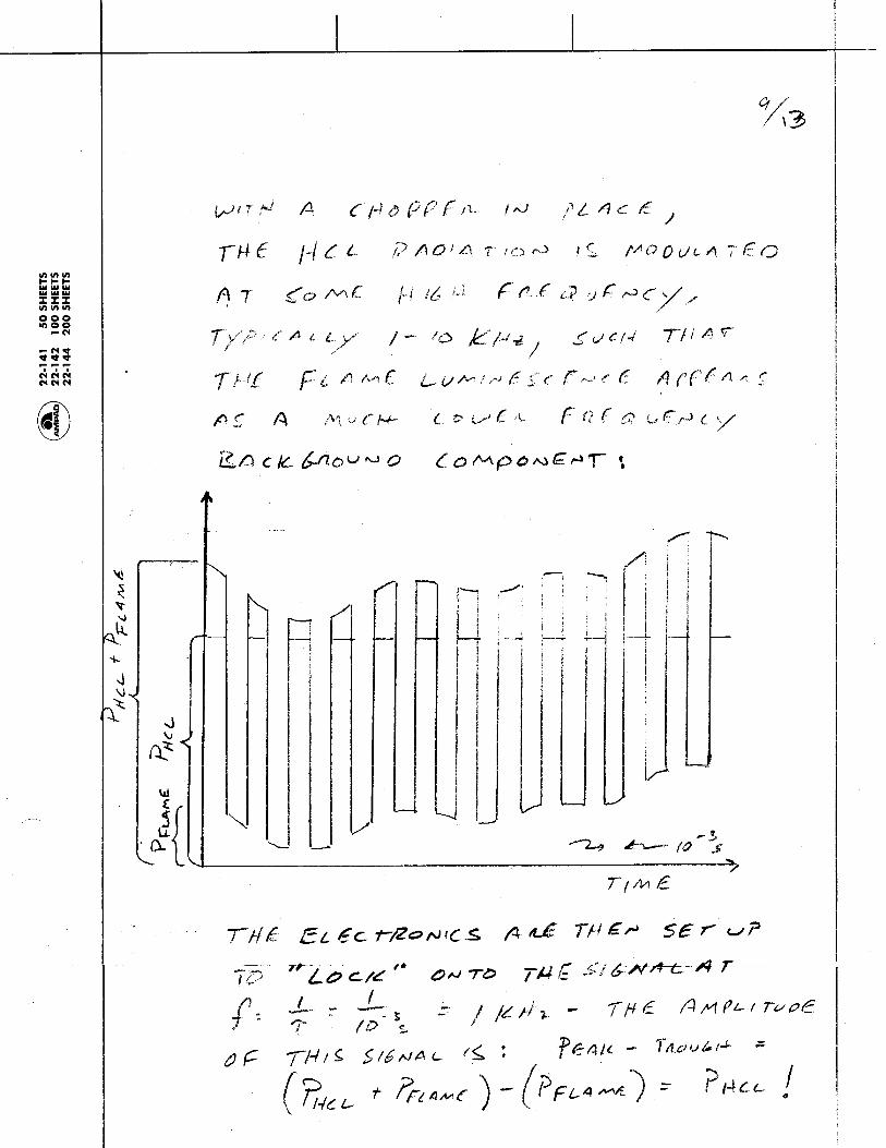
Chem 155 Unit 7 Page 145 of 316
Page 145 of 316
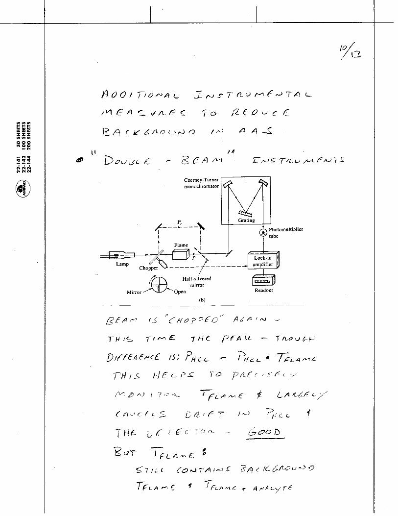
Chem 155 Unit 7 Page 146 of 316
Page 146 of 316
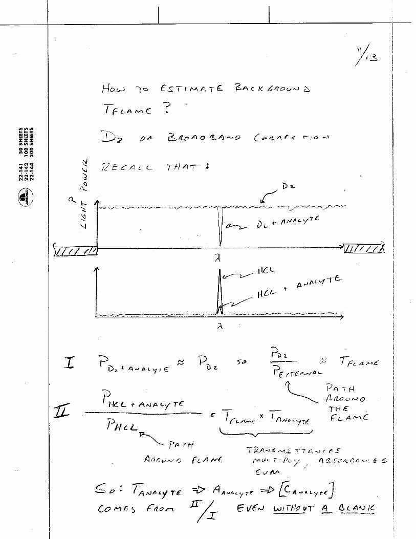
Chem 155 Unit 7 Page 147 of 316
Page 147 of 316
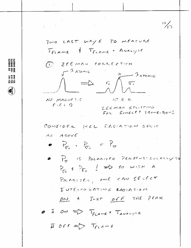
Chem 155 Unit 7 Page 148 of 316
Page 148 of 316
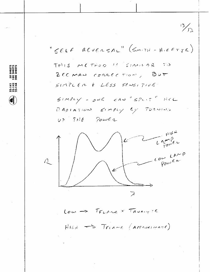
Chem 155 Unit 7 Page 149 of 316
Page 149 of 316
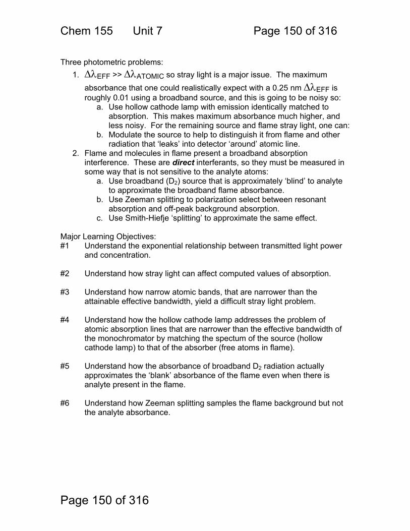
Chem 155 Unit 7 Page 150 of 316
Page 150 of 316
Three photometric problems:
1. ΔλEFF >> ΔλATOMIC so stray light is a major issue. The maximum absorbance that one could realistically expect with a 0.25 nm ΔλEFF is roughly 0.01 using a broadband source, and this is going to be noisy so:
a. Use hollow cathode lamp with emission identically matched to absorption. This makes maximum absorbance much higher, and less noisy. For the remaining source and flame stray light, one can:
b. Modulate the source to help to distinguish it from flame and other radiation that ‘leaks’ into detector ‘around’ atomic line.
2. Flame and molecules in flame present a broadband absorption interference. These are direct interferants, so they must be measured in some way that is not sensitive to the analyte atoms:
a. Use broadband (D2) source that is approximately ‘blind’ to analyte to approximate the broadband flame absorbance.
b. Use Zeeman splitting to polarization select between resonant absorption and off-peak background absorption.
c. Use Smith-Hiefje ‘splitting’ to approximate the same effect. Major Learning Objectives: #1 Understand the exponential relationship between transmitted light power
and concentration. #2 Understand how stray light can affect computed values of absorption. #3 Understand how narrow atomic bands, that are narrower than the
attainable effective bandwidth, yield a difficult stray light problem. #4 Understand how the hollow cathode lamp addresses the problem of
atomic absorption lines that are narrower than the effective bandwidth of the monochromator by matching the spectum of the source (hollow cathode lamp) to that of the absorber (free atoms in flame).
#5 Understand how the absorbance of broadband D2 radiation actually
approximates the ‘blank’ absorbance of the flame even when there is analyte present in the flame.
#6 Understand how Zeeman splitting samples the flame background but not
the analyte absorbance.
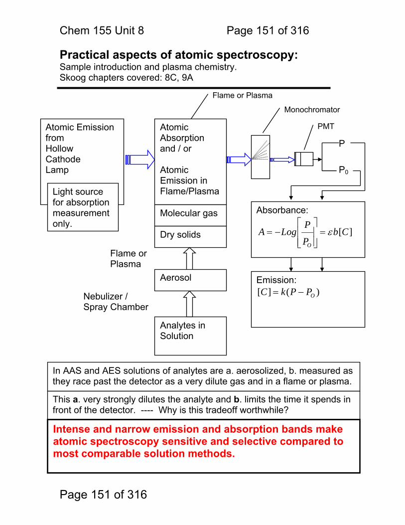
Chem 155 Unit 8 Page 151 of 316
Page 151 of 316
In AAS and AES solutions of analytes are a. aerosolized, b. measured as they race past the detector as a very dilute gas and in a flame or plasma.
Practical aspects of atomic spectroscopy: Sample introduction and plasma chemistry. Skoog chapters covered: 8C, 9A
Absorbance:
][CbP
PLogA
O
ε=⎥⎥⎦
⎤
⎢⎢⎣
⎡−=
Emission: )(][ OPPkC −=
Atomic Emission from Hollow Cathode Lamp
Atomic Absorption and / or Atomic Emission in Flame/Plasma
Dry solids
Analytes in Solution
Aerosol
Molecular gas
Monochromator
PMT
P
P0
Nebulizer / Spray Chamber
Flame or Plasma
Light source for absorption measurement only.
Flame or Plasma
Intense and narrow emission and absorption bands make atomic spectroscopy sensitive and selective compared to most comparable solution methods.
This a. very strongly dilutes the analyte and b. limits the time it spends in front of the detector. ---- Why is this tradeoff worthwhile?
Chem 155 Unit 8 Page 152 of 316
Page 152 of 316
Nebulization (sample introduction): Sample introduction in AAS and AES is usually through a nebulizer. The nebulizer makes a very fine mist of the analyte solution. The finest droplets in this mist are then selected by the spray chamber. These droplets are then swept into the flame or plasma. This sample introduction process is necessary but: a. b. c.
inefficient
problematic
hard to do reproducibly
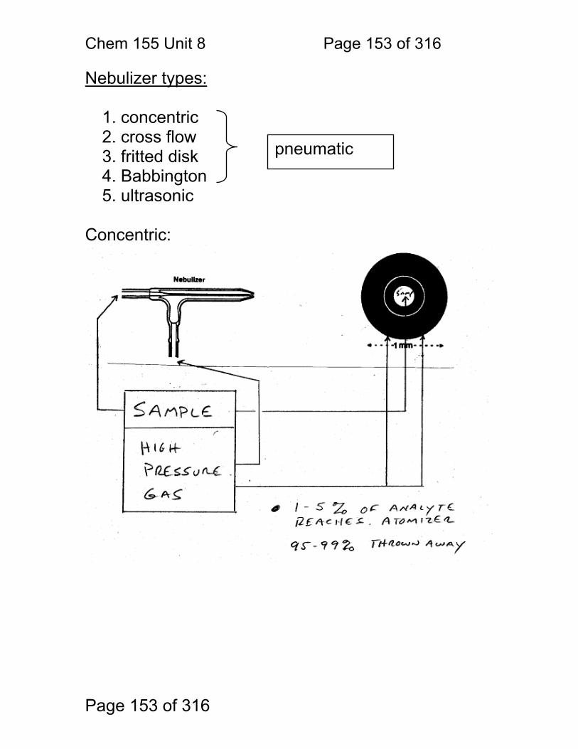
Chem 155 Unit 8 Page 153 of 316
Page 153 of 316
Nebulizer types:
1. concentric 2. cross flow 3. fritted disk 4. Babbington 5. ultrasonic
Concentric:
pneumatic
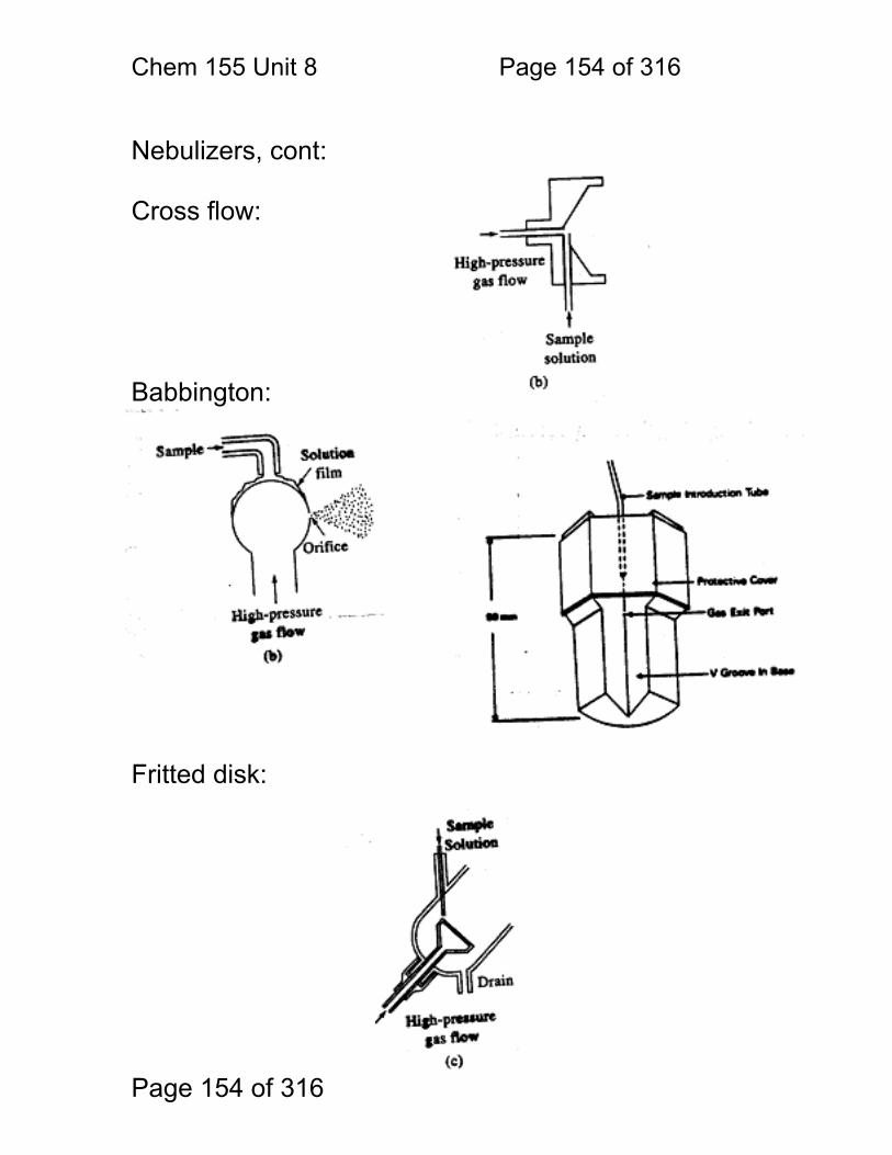
Chem 155 Unit 8 Page 154 of 316
Page 154 of 316
Nebulizers, cont: Cross flow: Babbington:
Fritted disk:
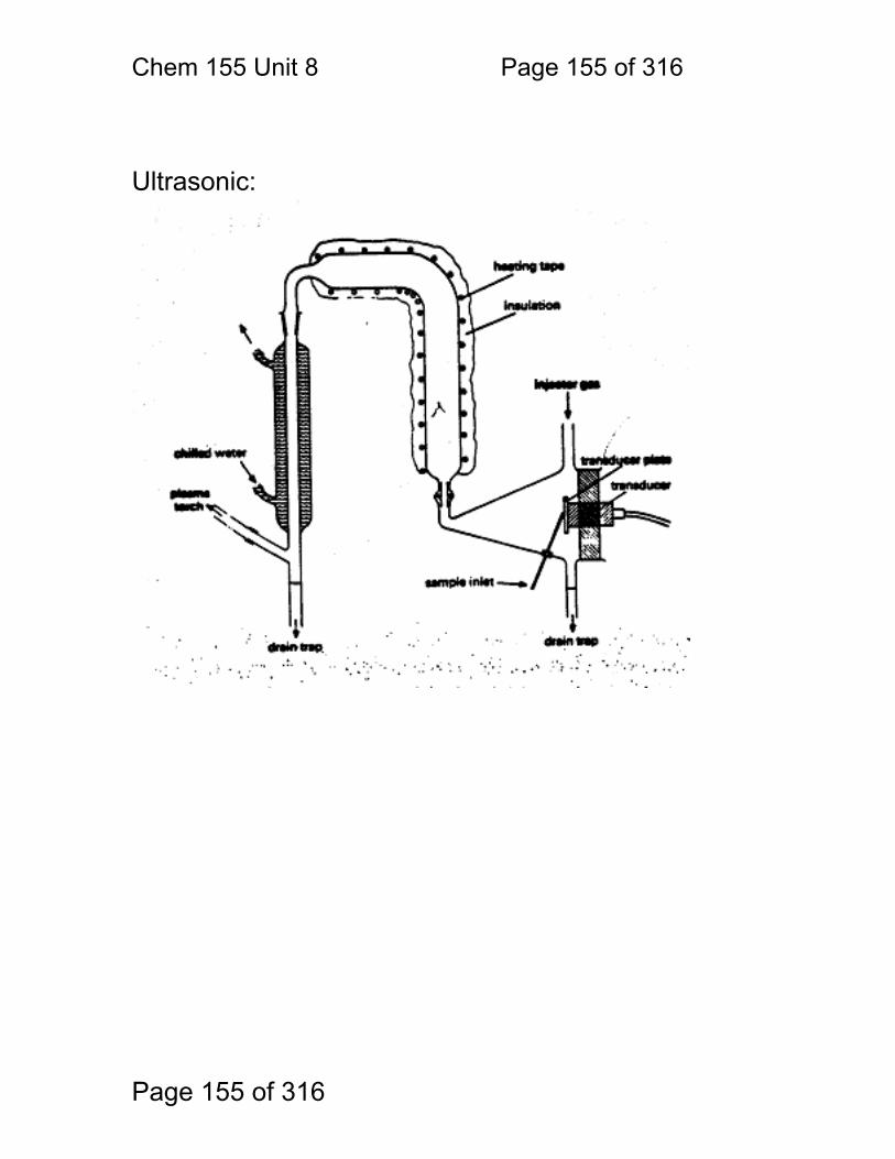
Chem 155 Unit 8 Page 155 of 316
Page 155 of 316
Ultrasonic:
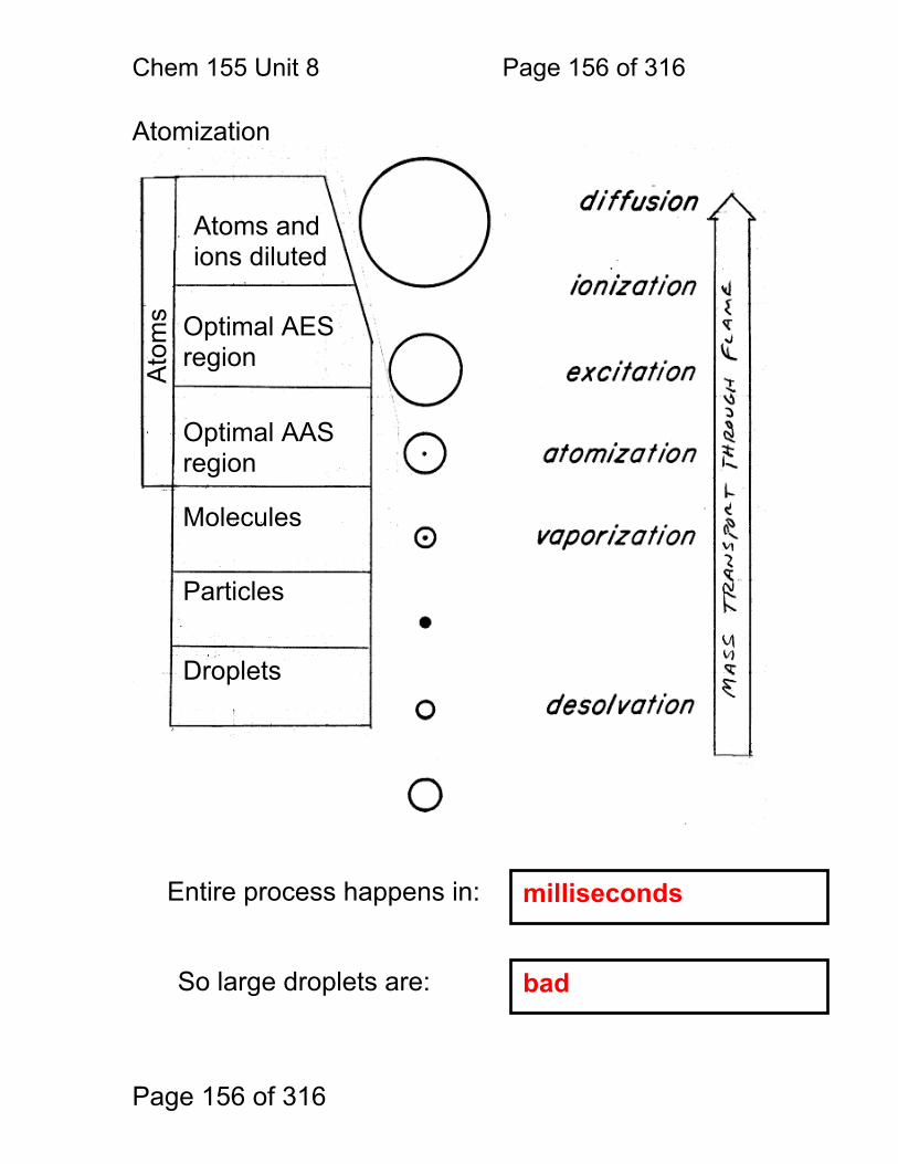
Chem 155 Unit 8 Page 156 of 316
Page 156 of 316
Atomization
Droplets
Particles
Molecules
Optimal AAS region
Optimal AES region
Atoms and ions diluted
Ato
ms
Entire process happens in:
So large droplets are: bad
milliseconds
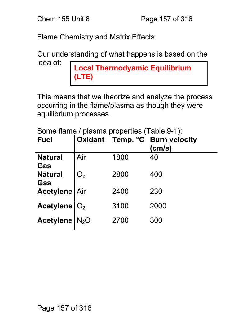
Chem 155 Unit 8 Page 157 of 316
Page 157 of 316
Flame Chemistry and Matrix Effects Our understanding of what happens is based on the idea of: This means that we theorize and analyze the process occurring in the flame/plasma as though they were equilibrium processes. Some flame / plasma properties (Table 9-1): Fuel Oxidant Temp. °C Burn velocity
(cm/s) Natural Gas
Air 1800 40
Natural Gas
O2 2800 400
Acetylene Air 2400 230
Acetylene O2 3100 2000
Acetylene N2O 2700 300
Local Thermodyamic Equilibrium (LTE)
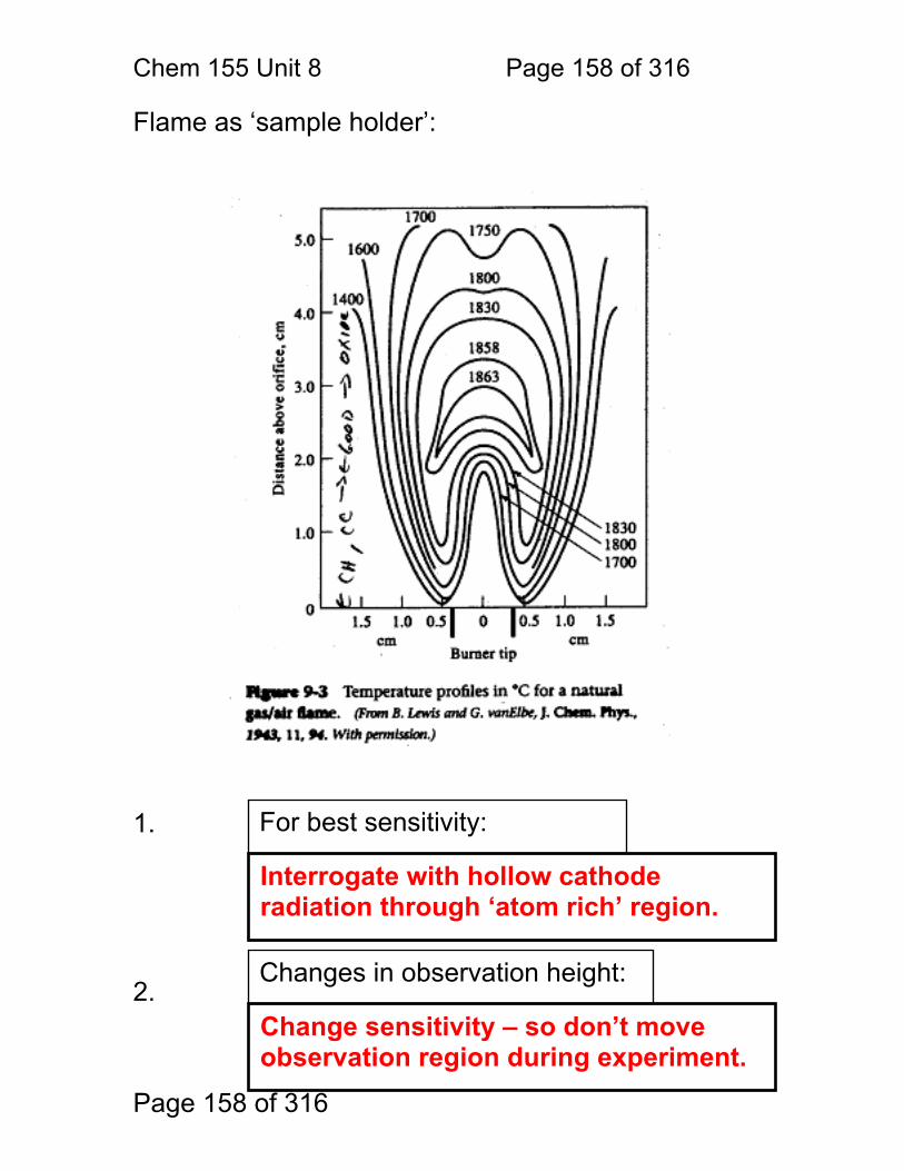
Chem 155 Unit 8 Page 158 of 316
Page 158 of 316
Flame as ‘sample holder’:
1.
2.
Interrogate with hollow cathode radiation through ‘atom rich’ region.
For best sensitivity:
Change sensitivity – so don’t move observation region during experiment.
Changes in observation height:
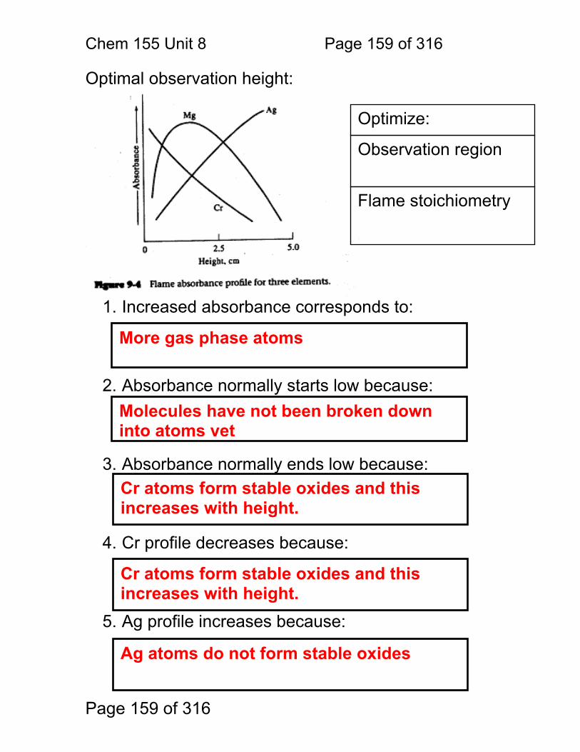
Chem 155 Unit 8 Page 159 of 316
Page 159 of 316
Optimal observation height:
1. Increased absorbance corresponds to:
2. Absorbance normally starts low because:
3. Absorbance normally ends low because:
4. Cr profile decreases because: 5. Ag profile increases because:
More gas phase atoms
Cr atoms form stable oxides and this increases with height.
Molecules have not been broken down into atoms yet
Cr atoms form stable oxides and this increases with height.
Ag atoms do not form stable oxides
Optimize:
Observation region
Flame stoichiometry
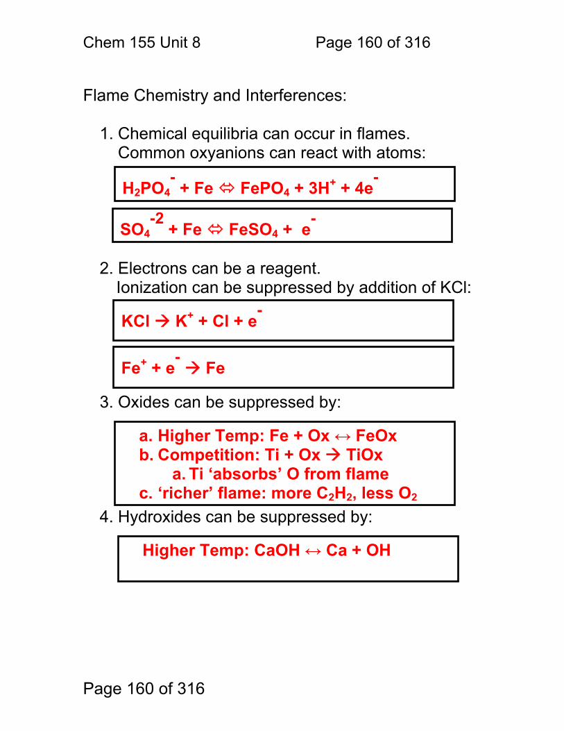
Chem 155 Unit 8 Page 160 of 316
Page 160 of 316
Flame Chemistry and Interferences:
1. Chemical equilibria can occur in flames.
Common oxyanions can react with atoms: 2. Electrons can be a reagent.
Ionization can be suppressed by addition of KCl:
3. Oxides can be suppressed by: 4. Hydroxides can be suppressed by:
H2PO4-
+ Fe FePO4 + 3H+ + 4e-
SO4-2
+ Fe FeSO4 + e-
KCl K+ + Cl + e-
Fe+ + e- Fe
a. Higher Temp: Fe + Ox ↔ FeOx b. Competition: Ti + Ox TiOx
a. Ti ‘absorbs’ O from flame c. ‘richer’ flame: more C2H2, less O2
Higher Temp: CaOH ↔ Ca + OH
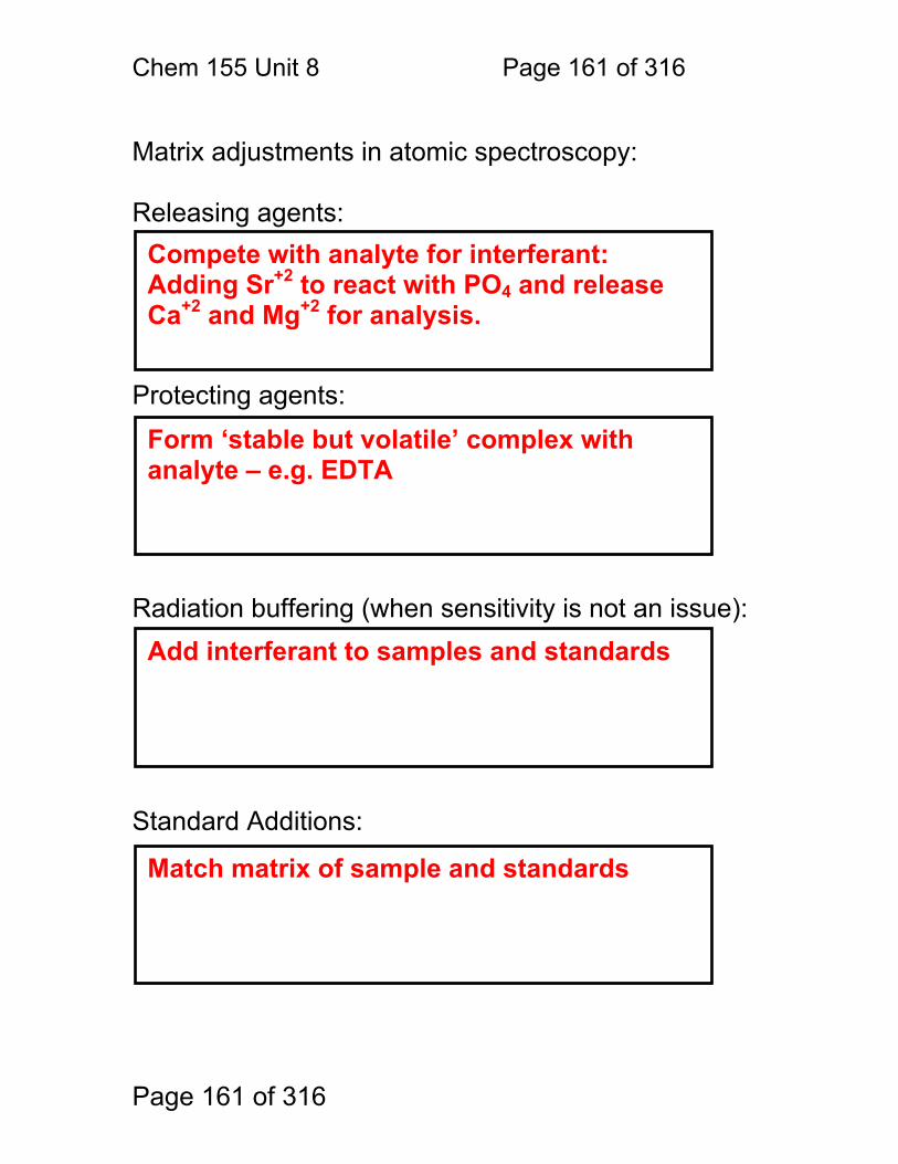
Chem 155 Unit 8 Page 161 of 316
Page 161 of 316
Matrix adjustments in atomic spectroscopy: Releasing agents:
Protecting agents:
Radiation buffering (when sensitivity is not an issue):
Standard Additions:
Compete with analyte for interferant: Adding Sr+2 to react with PO4 and release Ca+2 and Mg+2 for analysis.
Form ‘stable but volatile’ complex with analyte – e.g. EDTA
Add interferant to samples and standards
Match matrix of sample and standards
Chem 155 Unit 9 Atomic Emission Page 162 of 316
Page 162 of 316
Atomic Emission Spectroscopy Responsibilities in the Chapter: Introduction and all of 10A • Overview Nomenclature
Plasma Types Pro’s and Con’s
• Inductively Coupled Plasma Torch Design Operating Principles Plasma Properties Plasma Optimization
• Direct Current Plasma Design Properties
• Spectrometers Bandwidth Considerations Multi-channel Designs
• Quantitation and Accuracy • Comparisons with Atomic Absorption
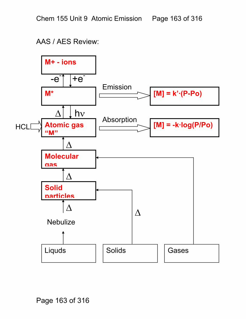
Chem 155 Unit 9 Atomic Emission Page 163 of 316
Page 163 of 316
AAS / AES Review:
Solids Gases Liquds
Solid particles
Molecular gas
Atomic gas “M”
M*
M+ - ions
HCL
[M] = k’·(P-Po)
Nebulize
Absorption
Emission
Δ
Δ
Δ
Δ
Δ hν [M] = -k·log(P/Po)
-e- +e-
Chem 155 Unit 9 Atomic Emission Page 164 of 316
Page 164 of 316
Types of AES: 1.1.54 PLASMA
Plasma is ionized gas – typically Ar, Ar+, e- Ionization is maintained in one of three ways:
• A DC electrical discharge called “Direct Current Plasma”, DCP or Plasma Jet
• An induction coil operating at 27 or 41 MHz “Inductively Coupled Plasma” , ICP
• A Microwave Cavity called Microwave Induced Plasma or MIP
1.1.55 FLAME
• Flame Emission Spectrometry or “FES” • Flame is “chemical plasma” – typically
comprising CO2, H2O, other Molecules, e- e- • Flame types include: Air - C2H2 , N2O - C2H2 ,
O2 – C2H2 • FES is limited to easily excited species such as
Na, Li, K 1.1.56 ARC / SPARK
• Arc = Continuous Discharge • Spark = Pulsed Discharge • These two are like DCP, but are done in air, on
solids (e.g. pressed powders) or metal surfaces
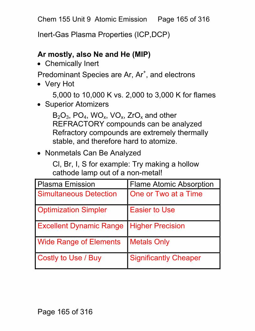
Chem 155 Unit 9 Atomic Emission Page 165 of 316
Page 165 of 316
Inert-Gas Plasma Properties (ICP,DCP) Ar mostly, also Ne and He (MIP) • Chemically Inert Predominant Species are Ar, Ar+, and electrons • Very Hot
5,000 to 10,000 K vs. 2,000 to 3,000 K for flames • Superior Atomizers
B2O3, PO4, WOx, VOx, ZrOx and other REFRACTORY compounds can be analyzed Refractory compounds are extremely thermally stable, and therefore hard to atomize.
• Nonmetals Can Be Analyzed Cl, Br, I, S for example: Try making a hollow cathode lamp out of a non-metal!
Plasma Emission Flame Atomic Absorption Simultaneous Detection One or Two at a Time
Optimization Simpler Easier to Use
Excellent Dynamic Range Higher Precision
Wide Range of Elements Metals Only
Costly to Use / Buy Significantly Cheaper
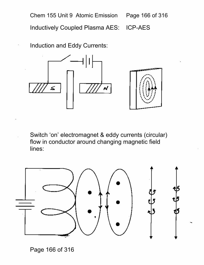
Chem 155 Unit 9 Atomic Emission Page 166 of 316
Page 166 of 316
Inductively Coupled Plasma AES: ICP-AES Induction and Eddy Currents: Switch ‘on’ electromagnet & eddy currents (circular) flow in conductor around changing magnetic field lines:
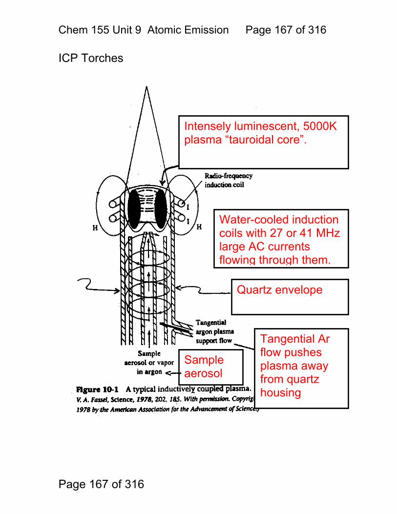
Chem 155 Unit 9 Atomic Emission Page 167 of 316
Page 167 of 316
ICP Torches
Intensely luminescent, 5000K plasma “tauroidal core”.
Water-cooled induction coils with 27 or 41 MHz large AC currents flowing through them.
Quartz envelope
Tangential Ar flow pushes plasma away from quartz housing
Sample aerosol
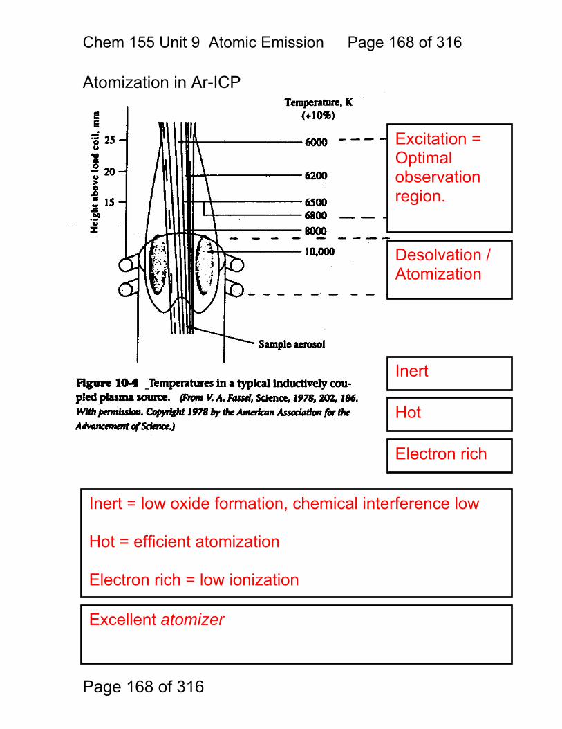
Chem 155 Unit 9 Atomic Emission Page 168 of 316
Page 168 of 316
Atomization in Ar-ICP
Analyte Atomization / Ionization:
Properties:
Excitation = Optimal observation region.
Desolvation / Atomization
Inert
Inert = low oxide formation, chemical interference low Hot = efficient atomization Electron rich = low ionization
Hot
Electron rich
Excellent atomizer
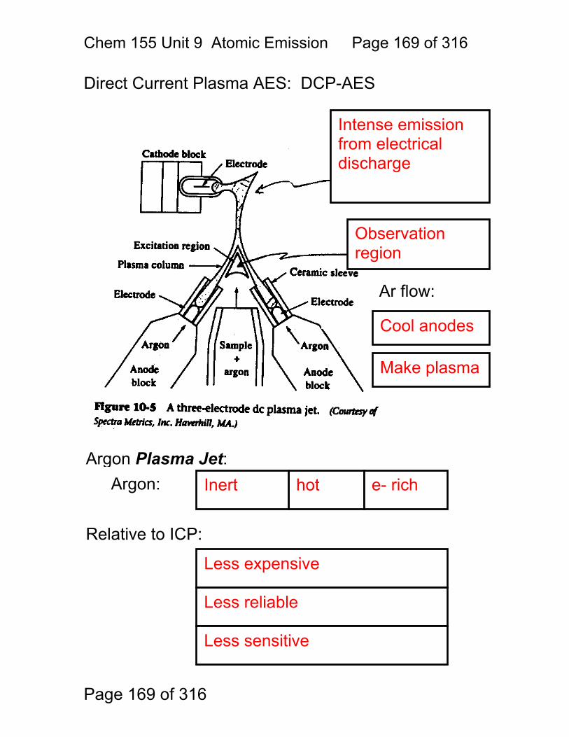
Chem 155 Unit 9 Atomic Emission Page 169 of 316
Page 169 of 316
Direct Current Plasma AES: DCP-AES
Observation region
Intense emission from electrical discharge
Ar flow:
Cool anodes
Make plasma
Argon Plasma Jet: Argon: hot e- rich Inert
Less expensive
Relative to ICP:
Less reliable
Less sensitive
Chem 155 Unit 9 Atomic Emission Page 170 of 316
Page 170 of 316
Advantages of Emission Methods One of the main advantages of emission methods is:
With the appropriate spectrometer design, it is possible to measure many elements at once using emission. This means:
With conventional spectrometers, this means many photomultiplier tubes (PMT’s) placed along the focal plane of the Czerny-Turner, or similar monochromator. But, PMT’s are neither small, nor cheap. So, PMT-based multi-channel spectrometers are both BIG, and EXPENSIVE. With the echelle design, there is a 2-dimensional focal plane that happens to be extremely well suited to the lithographically designed semiconductor charge-transfer array detector such as the CCD and CID.
Simultaneous multielement determinations
Simultaneous light detection at different wavelengths – i.e. different points along the focal plane.
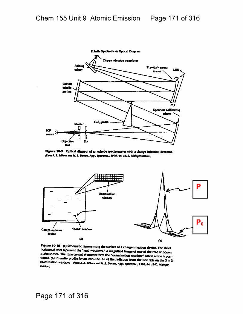
Chem 155 Unit 9 Atomic Emission Page 171 of 316
Page 171 of 316
P
P0
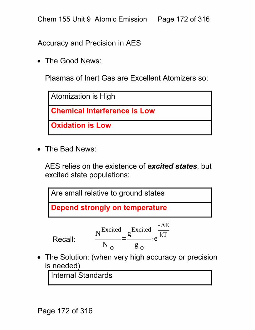
Chem 155 Unit 9 Atomic Emission Page 172 of 316
Page 172 of 316
NExcited
N o
gExcited
g oe
ΔEkT.
Accuracy and Precision in AES • The Good News:
Plasmas of Inert Gas are Excellent Atomizers so:
Atomization is High
Chemical Interference is Low
Oxidation is Low
• The Bad News:
AES relies on the existence of excited states, but excited state populations:
Are small relative to ground states
Depend strongly on temperature
Recall:
• The Solution: (when very high accuracy or precision is needed)
Internal Standards
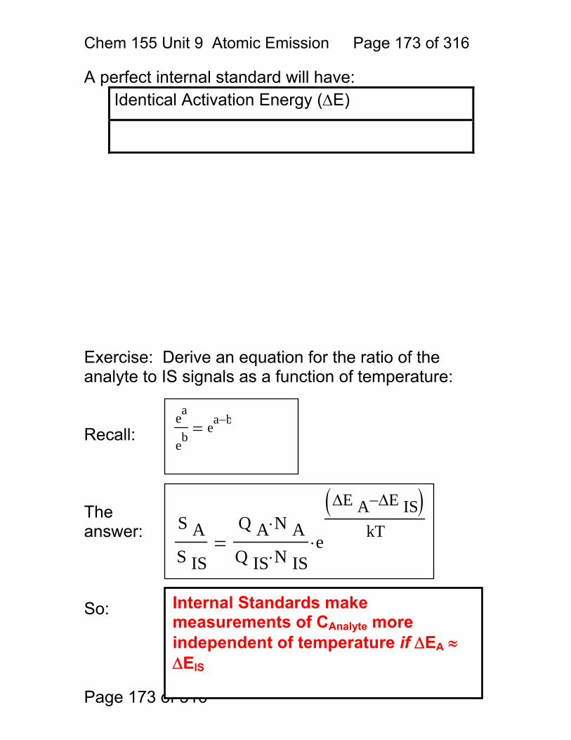
Chem 155 Unit 9 Atomic Emission Page 173 of 316
Page 173 of 316
Internal Standards make measurements of CAnalyte more independent of temperature if ΔEA ≈ ΔEIS
A perfect internal standard will have: Identical Activation Energy (ΔE)
Exercise: Derive an equation for the ratio of the analyte to IS signals as a function of temperature: Recall: The answer: So:
ea
ebea b−
S AS IS
Q A N A⋅
Q IS N IS⋅e
ΔE A ΔE IS−( )kT
⋅
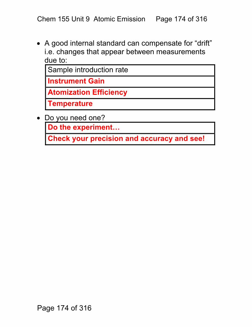
Chem 155 Unit 9 Atomic Emission Page 174 of 316
Page 174 of 316
• A good internal standard can compensate for “drift”
i.e. changes that appear between measurements due to: Sample introduction rate Instrument Gain Atomization Efficiency Temperature
• Do you need one? Do the experiment… Check your precision and accuracy and see!
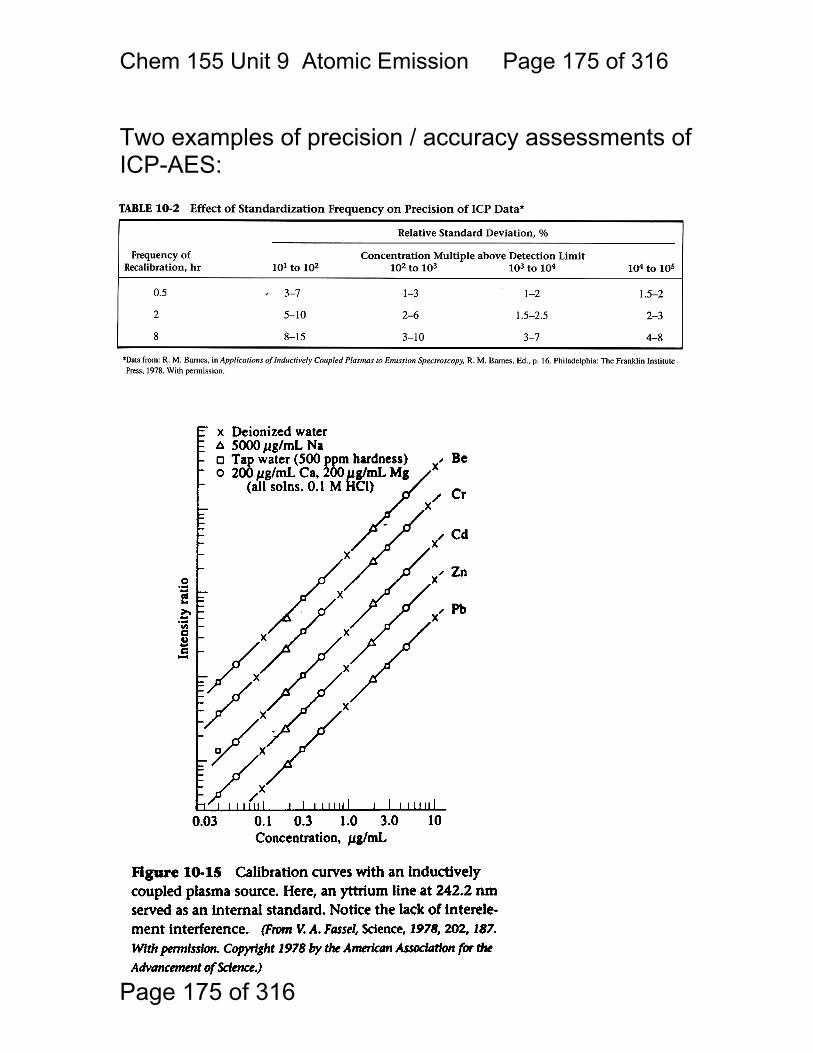
Chem 155 Unit 9 Atomic Emission Page 175 of 316
Page 175 of 316
Two examples of precision / accuracy assessments of ICP-AES:
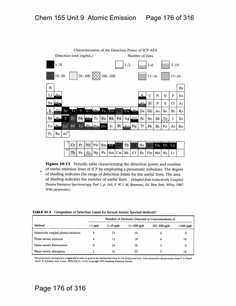
Chem 155 Unit 9 Atomic Emission Page 176 of 316
Page 176 of 316
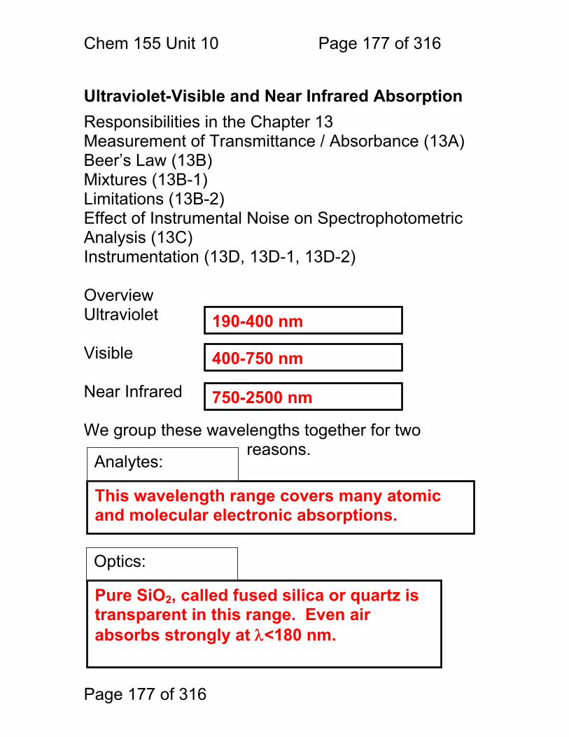
Chem 155 Unit 10 Page 177 of 316
Page 177 of 316
400-750 nm
750-2500 nm
This wavelength range covers many atomic and molecular electronic absorptions.
Pure SiO2, called fused silica or quartz is transparent in this range. Even air absorbs strongly at λ<180 nm.
190-400 nm
Ultraviolet-Visible and Near Infrared Absorption
Responsibilities in the Chapter 13 Measurement of Transmittance / Absorbance (13A) Beer’s Law (13B) Mixtures (13B-1) Limitations (13B-2) Effect of Instrumental Noise on Spectrophotometric Analysis (13C) Instrumentation (13D, 13D-1, 13D-2) Overview Ultraviolet Visible Near Infrared We group these wavelengths together for two
reasons.
Analytes:
Optics:
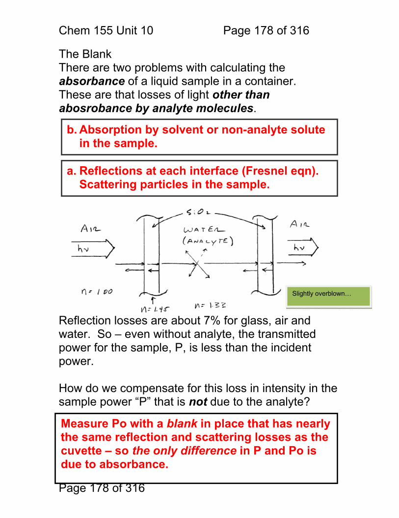
Chem 155 Unit 10 Page 178 of 316
Page 178 of 316
The Blank There are two problems with calculating the absorbance of a liquid sample in a container. These are that losses of light other than abosrobance by analyte molecules.
Reflection losses are about 7% for glass, air and water. So – even without analyte, the transmitted power for the sample, P, is less than the incident power. How do we compensate for this loss in intensity in the sample power “P” that is not due to the analyte?
Measure Po with a blank in place that has nearly the same reflection and scattering losses as the cuvette – so the only difference in P and Po is due to absorbance.
b. Absorption by solvent or non-analyte solute in the sample.
a. Reflections at each interface (Fresnel eqn). Scattering particles in the sample.
Slightly overblown…
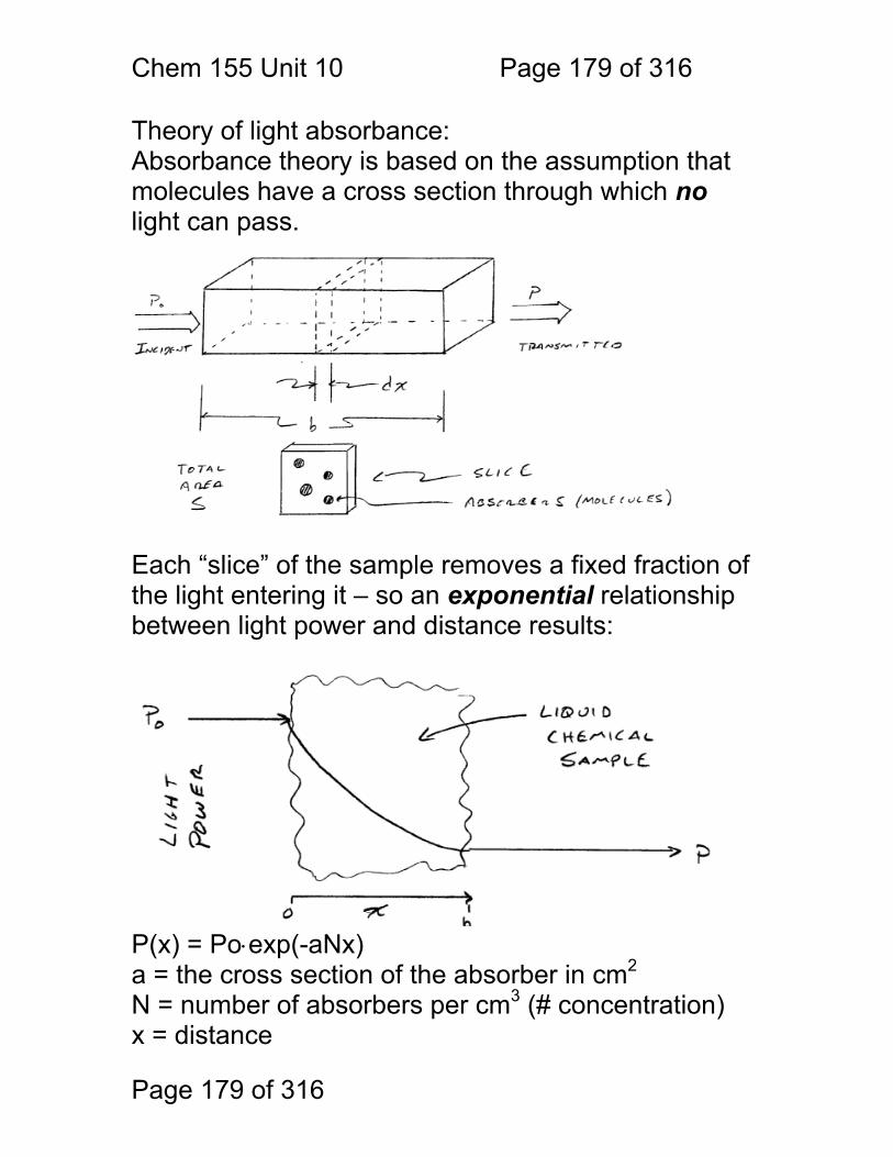
Chem 155 Unit 10 Page 179 of 316
Page 179 of 316
Theory of light absorbance: Absorbance theory is based on the assumption that molecules have a cross section through which no light can pass.
Each “slice” of the sample removes a fixed fraction of the light entering it – so an exponential relationship between light power and distance results:
P(x) = Po⋅exp(-aNx) a = the cross section of the absorber in cm2 N = number of absorbers per cm3 (# concentration) x = distance
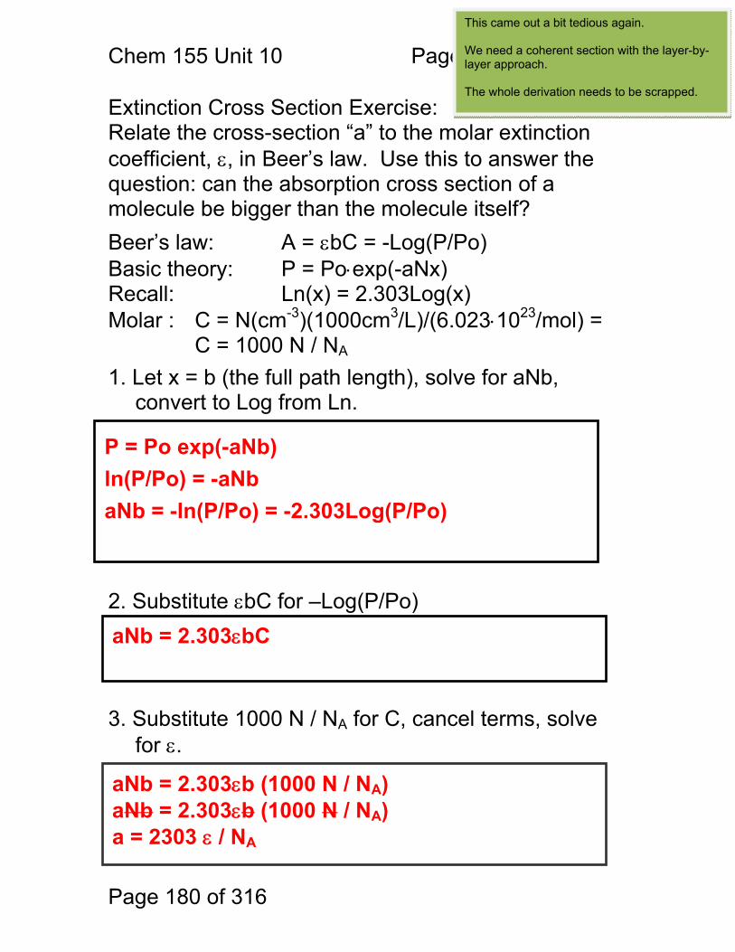
Chem 155 Unit 10 Page 180 of 316
Page 180 of 316
This came out a bit tedious again. We need a coherent section with the layer-by-layer approach. The whole derivation needs to be scrapped.
Extinction Cross Section Exercise: Relate the cross-section “a” to the molar extinction coefficient, ε, in Beer’s law. Use this to answer the question: can the absorption cross section of a molecule be bigger than the molecule itself? Beer’s law: A = εbC = -Log(P/Po) Basic theory: P = Po⋅exp(-aNx) Recall: Ln(x) = 2.303Log(x) Molar : C = N(cm-3)(1000cm3/L)/(6.023⋅1023/mol) =
C = 1000 N / NA 1. Let x = b (the full path length), solve for aNb,
convert to Log from Ln.
2. Substitute εbC for –Log(P/Po)
3. Substitute 1000 N / NA for C, cancel terms, solve
for ε.
P = Po exp(-aNb) ln(P/Po) = -aNb aNb = -ln(P/Po) = -2.303Log(P/Po)
aNb = 2.303εbC
aNb = 2.303εb (1000 N / NA) aNb = 2.303εb (1000 N / NA) a = 2303 ε / NA
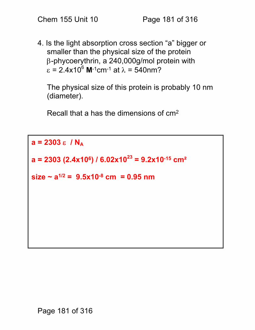
Chem 155 Unit 10 Page 181 of 316
Page 181 of 316
4. Is the light absorption cross section “a” bigger or
smaller than the physical size of the protein β-phycoerythrin, a 240,000g/mol protein with ε = 2.4x10⁶ M-1cm-1 at λ = 540nm?
The physical size of this protein is probably 10 nm (diameter).
Recall that a has the dimensions of cm2
a = 2303 ε / NA a = 2303 (2.4x10⁶) / 6.02x1023 = 9.2x10⁻¹⁵ cm² size ~ a1/2 = 9.5x10⁻⁸ cm = 0.95 nm
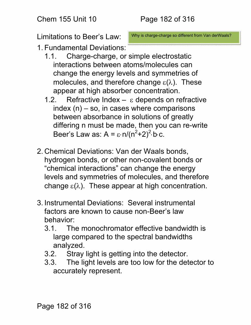
Chem 155 Unit 10 Page 182 of 316
Page 182 of 316
Limitations to Beer’s Law: 1. Fundamental Deviations:
1.1. Charge-charge, or simple electrostatic interactions between atoms/molecules can change the energy levels and symmetries of molecules, and therefore change ε(λ). These appear at high absorber concentration.
1.2. Refractive Index – ε depends on refractive index (n) – so, in cases where comparisons between absorbance in solutions of greatly differing n must be made, then you can re-write Beer’s Law as: A = ε⋅n/(n2+2)2⋅b⋅c.
2. Chemical Deviations: Van der Waals bonds,
hydrogen bonds, or other non-covalent bonds or “chemical interactions” can change the energy levels and symmetries of molecules, and therefore change ε(λ). These appear at high concentration.
3. Instrumental Deviations: Several instrumental
factors are known to cause non-Beer’s law behavior: 3.1. The monochromator effective bandwidth is
large compared to the spectral bandwidths analyzed.
3.2. Stray light is getting into the detector. 3.3. The light levels are too low for the detector to
accurately represent.
Why is charge-charge so different from Van derWaals?
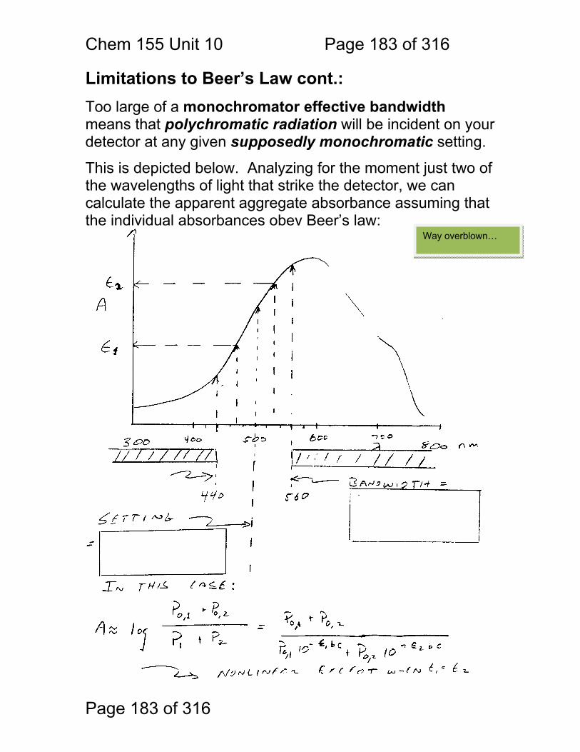
Chem 155 Unit 10 Page 183 of 316
Page 183 of 316
Limitations to Beer’s Law cont.:
Too large of a monochromator effective bandwidth means that polychromatic radiation will be incident on your detector at any given supposedly monochromatic setting.
This is depicted below. Analyzing for the moment just two of the wavelengths of light that strike the detector, we can calculate the apparent aggregate absorbance assuming that the individual absorbances obey Beer’s law: Way overblown…
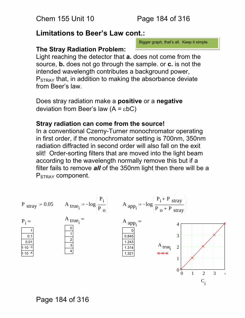
Chem 155 Unit 10 Page 184 of 316
Page 184 of 316
Limitations to Beer’s Law cont.: The Stray Radiation Problem: Light reaching the detector that a. does not come from the source, b. does not go through the sample. or c. is not the intended wavelength contributes a background power, PSTRAY that, in addition to making the absorbance deviate from Beer’s law. Does stray radiation make a positive or a negative deviation from Beer’s law (A = εbC) Stray radiation can come from the source! In a conventional Czerny-Turner monochromator operating in first order, if the monochromator setting is 700nm, 350nm radiation diffracted in second order will also fall on the exit slit! Order-sorting filters that are moved into the light beam according to the wavelength normally remove this but if a filter fails to remove all of the 350nm light then there will be a PSTRAY component.
P stray 0.05 A trueilog
PiP o
A appilog
Pi P strayP o P stray
0 1 2 3 40
1
2
3
4
A truei
Ci
A truei01234
=Pi1
0.10.01
1·10 -3
1·10 -4
= A appi0
0.8451.2431.3141.321
=
Bigger graph, that’s all. Keep it simple.
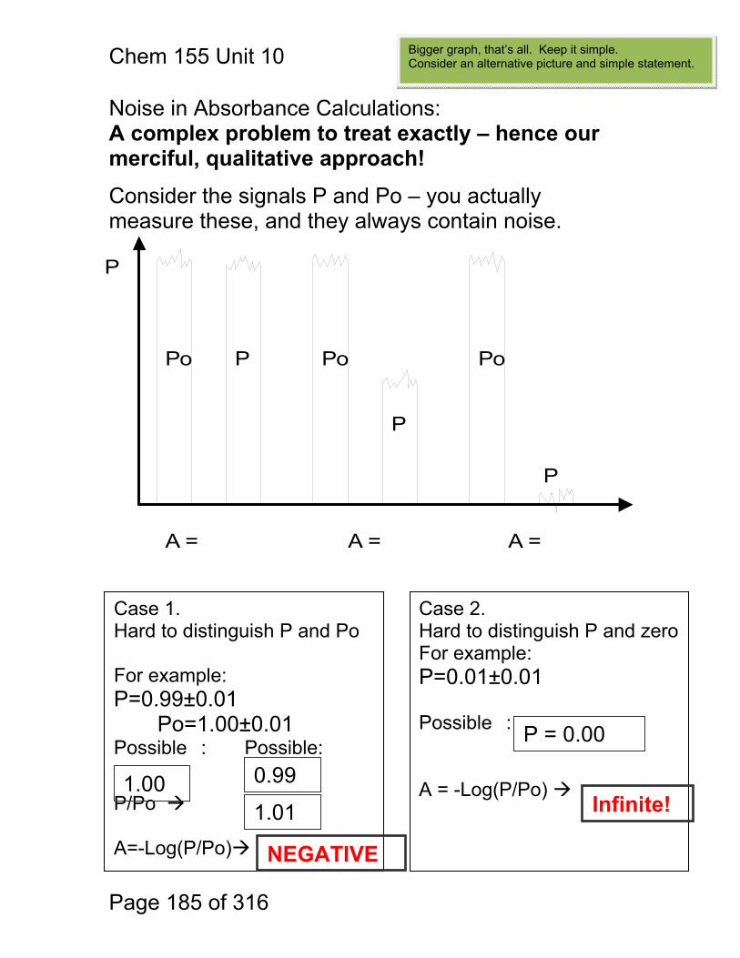
Chem 155 Unit 10 Page 185 of 316
Page 185 of 316
Noise in Absorbance Calculations: A complex problem to treat exactly – hence our merciful, qualitative approach!
Consider the signals P and Po – you actually measure these, and they always contain noise.
Po P Po
P
Po
P
A = A = A =
P
Case 1. Hard to distinguish P and Po For example: P=0.99±0.01 Po=1.00±0.01 Possible : Possible:
P/Po A=-Log(P/Po)
Case 2. Hard to distinguish P and zeroFor example: P=0.01±0.01 Possible : A = -Log(P/Po) 1.00 0.99
1.01
NEGATIVE
P = 0.00
Infinite!
Bigger graph, that’s all. Keep it simple. Consider an alternative picture and simple statement.
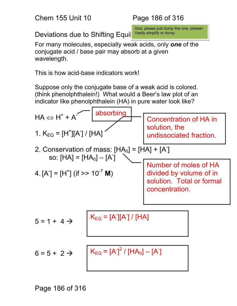
Chem 155 Unit 10 Page 186 of 316
Page 186 of 316
Deviations due to Shifting Equilibria: For many molecules, especially weak acids, only one of the conjugate acid / base pair may absorb at a given wavelength. This is how acid-base indicators work! Suppose only the conjugate base of a weak acid is colored. (think phenolphthalein!) What would a Beer’s law plot of an indicator like phenolphthalein (HA) in pure water look like? HA ⇔ H+ + A- 1. KEQ = [H+][A-] / [HA] 2. Conservation of mass: [HA0] = [HA] + [A-] so: [HA] = [HA0] – [A-] 4. [A-] = [H+] (if >> 10-7 M) 5 = 1 + 4 6 = 5 + 2
Concentration of HA in solution, the undissociated fraction.
Number of moles of HA divided by volume of in solution. Total or formal concentration.
KEQ = [A-][A-] / [HA]
KEQ = [A-]2 / [HA0] – [A-]
absorbing
God, please just dump this one, please! Vastly simplify or dump.
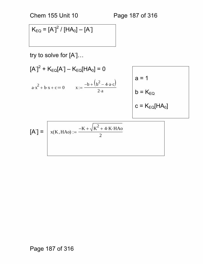
Chem 155 Unit 10 Page 187 of 316
Page 187 of 316
try to solve for [A-]… [A-]2 + KEQ[A-] – KEQ[HA0] = 0
a x2⋅ b x⋅+ c+ 0 xb− b2 4 a⋅ c⋅−( )+
2 a⋅:=
[A-] =
a = 1 b = KEQ c = KEQ[HA0]
KEQ = [A-]2 / [HA0] – [A-]
x K HAo,( )K− K2 4 K⋅ HAo⋅++
2:=
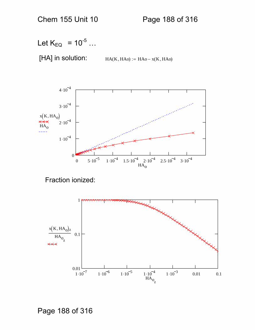
Chem 155 Unit 10 Page 188 of 316
Page 188 of 316
Let KEQ = 10-5 …
[HA] in solution: HA K HAo,( ) HAo x K HAo,( )−:=
0 5 .10 5 1 .10 4 1.5 .10 4 2 .10 4 2.5 .10 4 3 .10 40
1 .10 4
2 .10 4
3 .10 4
4 .10 4
x K HAo,( )HAo
HAo
Fraction ionized:
1 .10 7 1 .10 6 1 .10 5 1 .10 4 1 .10 3 0.01 0.10.01
0.1
1
x K HAo,( )z
HAoz
HAoz
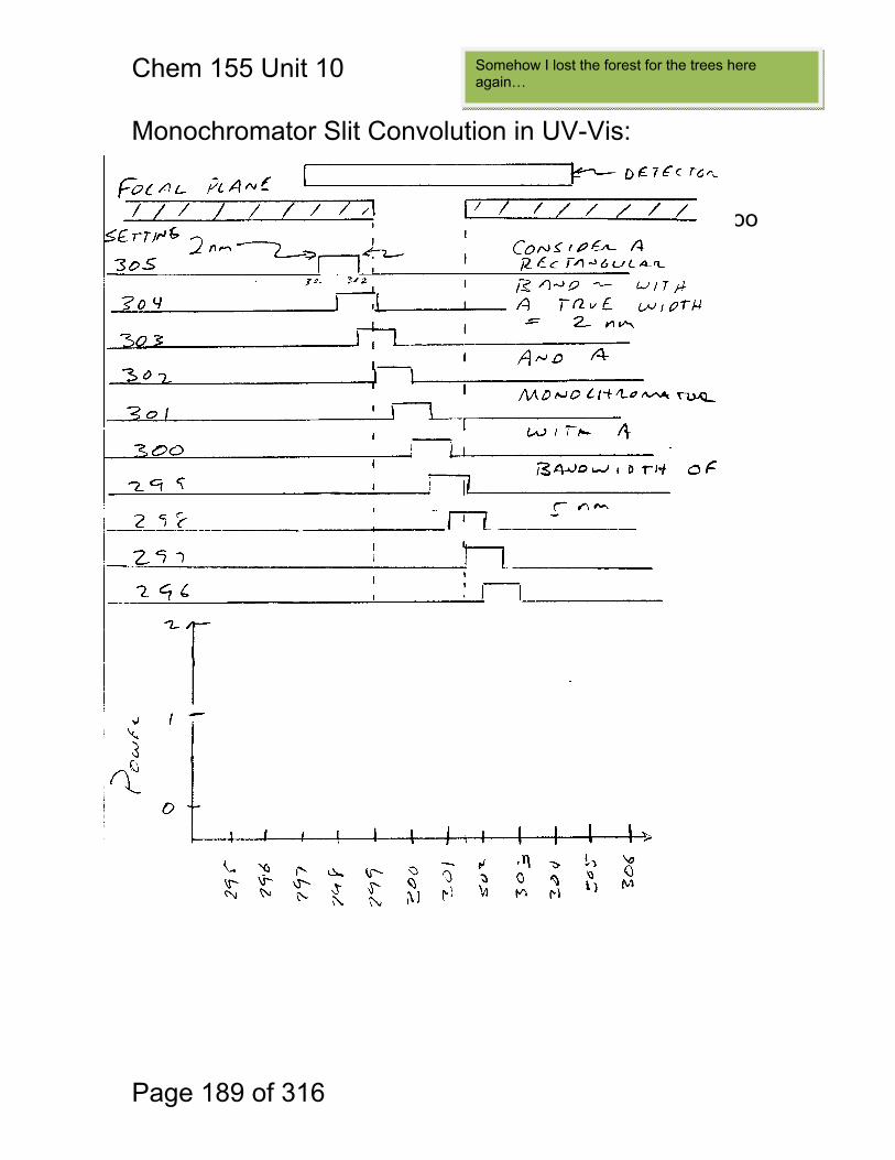
Chem 155 Unit 10 Page 189 of 316
Page 189 of 316
Monochromator Slit Convolution in UV-Vis: A monochromator may qualitatively distort absorbance peaks as well as quantitatively distort them if the ΔλEFF is too large.
Somehow I lost the forest for the trees here again…
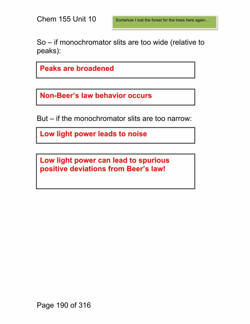
Chem 155 Unit 10 Page 190 of 316
Page 190 of 316
So – if monochromator slits are too wide (relative to peaks):
But – if the monochromator slits are too narrow:
Peaks are broadened
Non-Beer’s law behavior occurs
Low light power leads to noise
Low light power can lead to spurious positive deviations from Beer’s law!
Somehow I lost the forest for the trees here again…
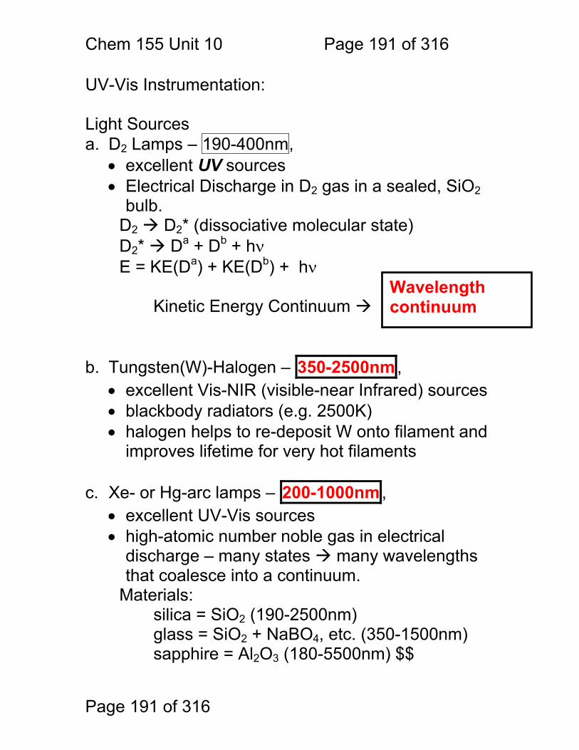
Chem 155 Unit 10 Page 191 of 316
Page 191 of 316
UV-Vis Instrumentation: Light Sources a. D2 Lamps – 190-400nm,
• excellent UV sources • Electrical Discharge in D2 gas in a sealed, SiO2
bulb. D2 D2* (dissociative molecular state) D2* Da + Db + hν E = KE(Da) + KE(Db) + hν Kinetic Energy Continuum
b. Tungsten(W)-Halogen – 350-2500nm , • excellent Vis-NIR (visible-near Infrared) sources • blackbody radiators (e.g. 2500K) • halogen helps to re-deposit W onto filament and
improves lifetime for very hot filaments
c. Xe- or Hg-arc lamps – 200-1000nm , • excellent UV-Vis sources • high-atomic number noble gas in electrical
discharge – many states many wavelengths that coalesce into a continuum.
Materials: silica = SiO2 (190-2500nm) glass = SiO2 + NaBO4, etc. (350-1500nm) sapphire = Al2O3 (180-5500nm) $$
Wavelength continuum
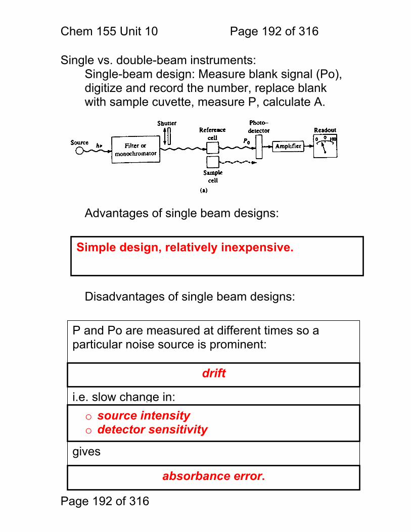
Chem 155 Unit 10 Page 192 of 316
Page 192 of 316
Single vs. double-beam instruments: Single-beam design: Measure blank signal (Po), digitize and record the number, replace blank with sample cuvette, measure P, calculate A. Advantages of single beam designs: Disadvantages of single beam designs:
Simple design, relatively inexpensive.
P and Po are measured at different times so a particular noise source is prominent:
i.e. slow change in:o source intensity o detector sensitivity
absorbance error.
drift
gives
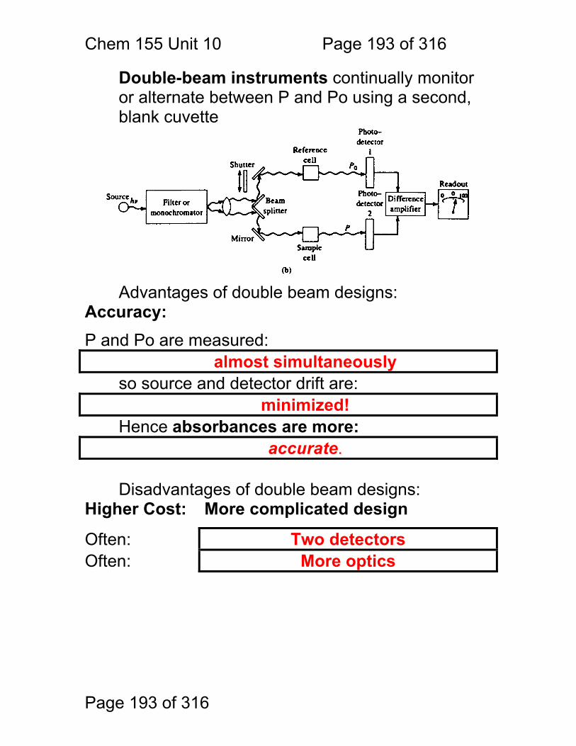
Chem 155 Unit 10 Page 193 of 316
Page 193 of 316
Double-beam instruments continually monitor or alternate between P and Po using a second, blank cuvette
Advantages of double beam designs: Accuracy: P and Po are measured:
almost simultaneously so source and detector drift are:
minimized! Hence absorbances are more:
accurate. Disadvantages of double beam designs:
Higher Cost: More complicated design
Often: Two detectors Often: More optics
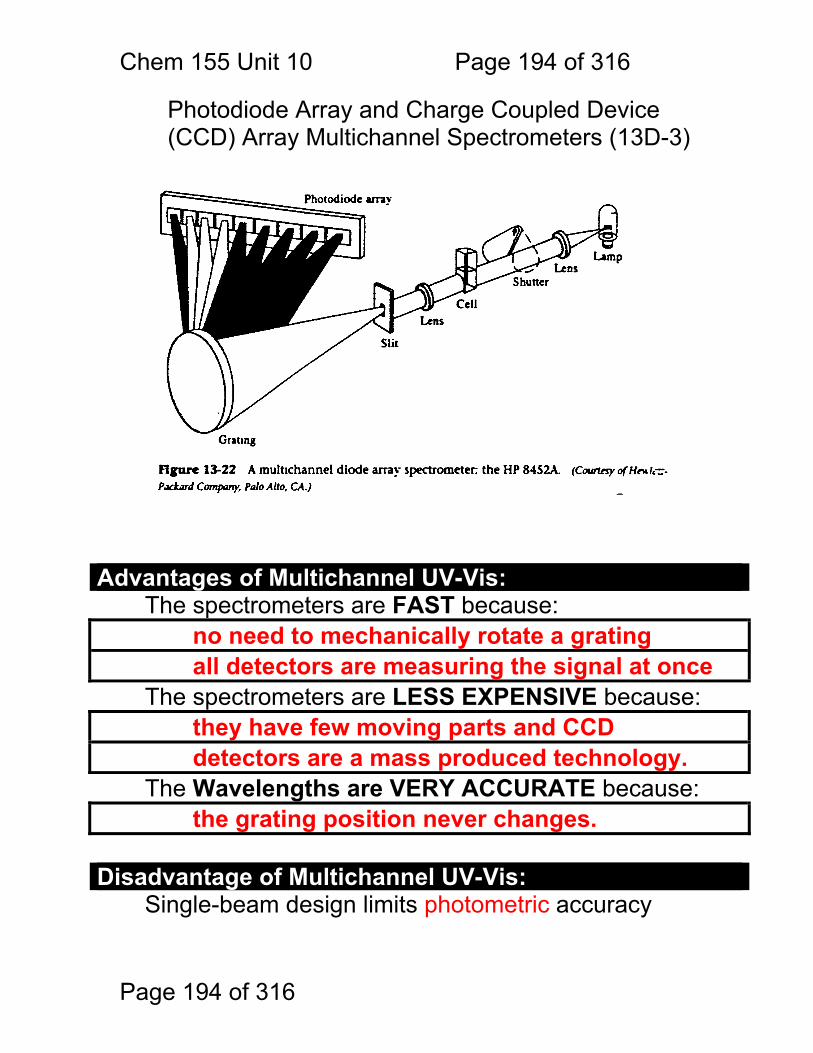
Chem 155 Unit 10 Page 194 of 316
Page 194 of 316
Photodiode Array and Charge Coupled Device (CCD) Array Multichannel Spectrometers (13D-3)
Advantages of Multichannel UV-Vis: The spectrometers are FAST because:
no need to mechanically rotate a grating all detectors are measuring the signal at once
The spectrometers are LESS EXPENSIVE because: they have few moving parts and CCD detectors are a mass produced technology.
The Wavelengths are VERY ACCURATE because: the grating position never changes.
Disadvantage of Multichannel UV-Vis:
Single-beam design limits photometric accuracy
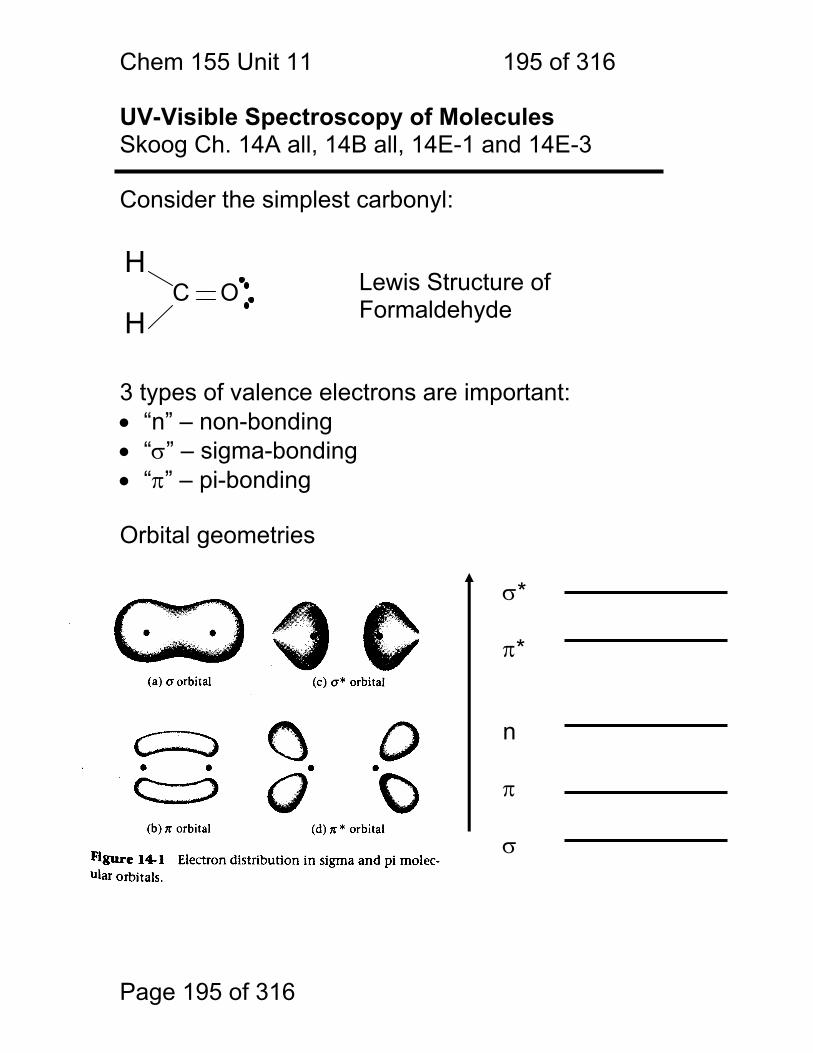
Chem 155 Unit 11 195 of 316
Page 195 of 316
UV-Visible Spectroscopy of Molecules Skoog Ch. 14A all, 14B all, 14E-1 and 14E-3 Consider the simplest carbonyl: Lewis Structure of Formaldehyde 3 types of valence electrons are important: • “n” – non-bonding • “σ” – sigma-bonding • “π” – pi-bonding Orbital geometries σ* π* n π σ
H C O H
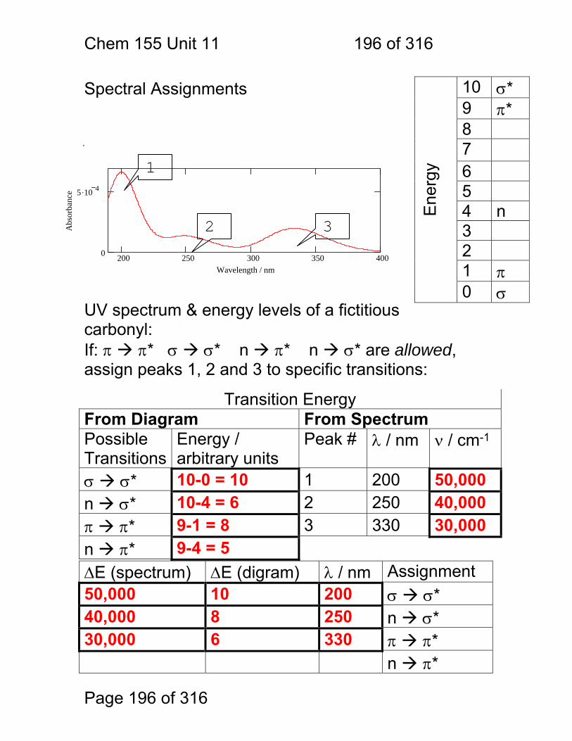
Chem 155 Unit 11 196 of 316
Page 196 of 316
Spectral Assignments
UV spectrum & energy levels of a fictitious carbonyl: If: π π* σ σ* n π* n σ* are allowed, assign peaks 1, 2 and 3 to specific transitions:
ΔE (spectrum) ΔE (digram) λ / nm Assignment 50,000 10 200 σ σ* 40,000 8 250 n σ* 30,000 6 330 π π* n π*
Ene
rgy
10 σ* 9 π* 8 7 6 5 4 n 3 2 1 π 0 σ
Transition Energy From Diagram From Spectrum Possible Transitions
Energy / arbitrary units
Peak # λ / nm ν / cm-1
σ σ* 10-0 = 10 1 200 50,000 n σ* 10-4 = 6 2 250 40,000 π π* 9-1 = 8 3 330 30,000 n π* 9-4 = 5
.
200 250 300 350 4000
5 .10 4
Wavelength / nm
Abs
orba
nce
1
2 3
Chem 155 Unit 11 197 of 316
Page 197 of 316
Classification of Electronic Transitions The following simplified classifications apply to organic molecules: 1. σ σ*
1.1. Highest energy! 1.2. Shortest wavelength λ < 200 nm 1.3. O2, N2, all molecules have σ-bonds so: this
radiation is absorbed by air and SiO2 so spectroscopy must be done in vacuum and is very difficult – called VUV or vacuum ultraviolet spectroscopy
2. n σ*
2.1. 150-250nm – most all transitions are found in the ultraviolet
2.2. Molecules with lone (nonbonding) pairs of electrons participate such as: O, N, Halogens
2.3. ε ∼ 100 to 1000 “medium” strength absorbers
3. n π*, π π* 3.1. Longest wavelength transitions 200-700 nm 3.2. Strongest absorbers ε ∼ 100 to 100,000 3.3. Limited to molecules with π-bonds – e.g.
alkenes, alkynes, aromatics, carbonyls, azides etc.
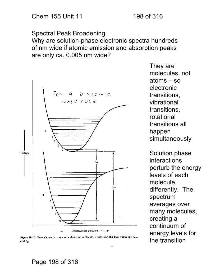
Chem 155 Unit 11 198 of 316
Page 198 of 316
Spectral Peak Broadening Why are solution-phase electronic spectra hundreds of nm wide if atomic emission and absorption peaks are only ca. 0.005 nm wide?
They are molecules, not atoms – so electronic transitions, vibrational transitions, rotational transitions all happen simultaneously Solution phase interactions perturb the energy levels of each molecule differently. The spectrum averages over many molecules, creating a continuum of energy levels for the transition
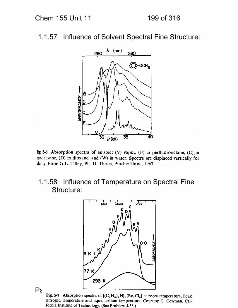
Chem 155 Unit 11 199 of 316
Page 199 of 316
1.1.57 Influence of Solvent Spectral Fine Structure: 1.1.58 Influence of Temperature on Spectral Fine
Structure:
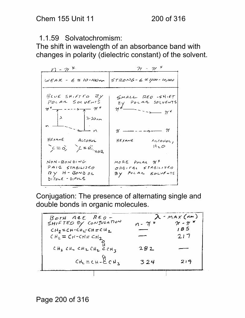
Chem 155 Unit 11 200 of 316
Page 200 of 316
1.1.59 Solvatochromism: The shift in wavelength of an absorbance band with changes in polarity (dielectric constant) of the solvent. Conjugation: The presence of alternating single and double bonds in organic molecules.
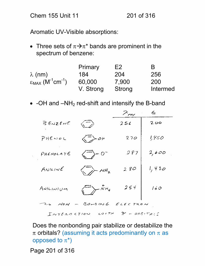
Chem 155 Unit 11 201 of 316
Page 201 of 316
Aromatic UV-Visible absorptions: • Three sets of π π* bands are prominent in the
spectrum of benzene: Primary E2 B λ (nm) 184 204 256 εMAX (M-1cm-1) 60,000 7,900 200 V. Strong Strong Intermed • -OH and –NH2 red-shift and intensify the B-band
Does the nonbonding pair stabilize or destabilize the π orbitals? (assuming it acts predominantly on π as opposed to π*)
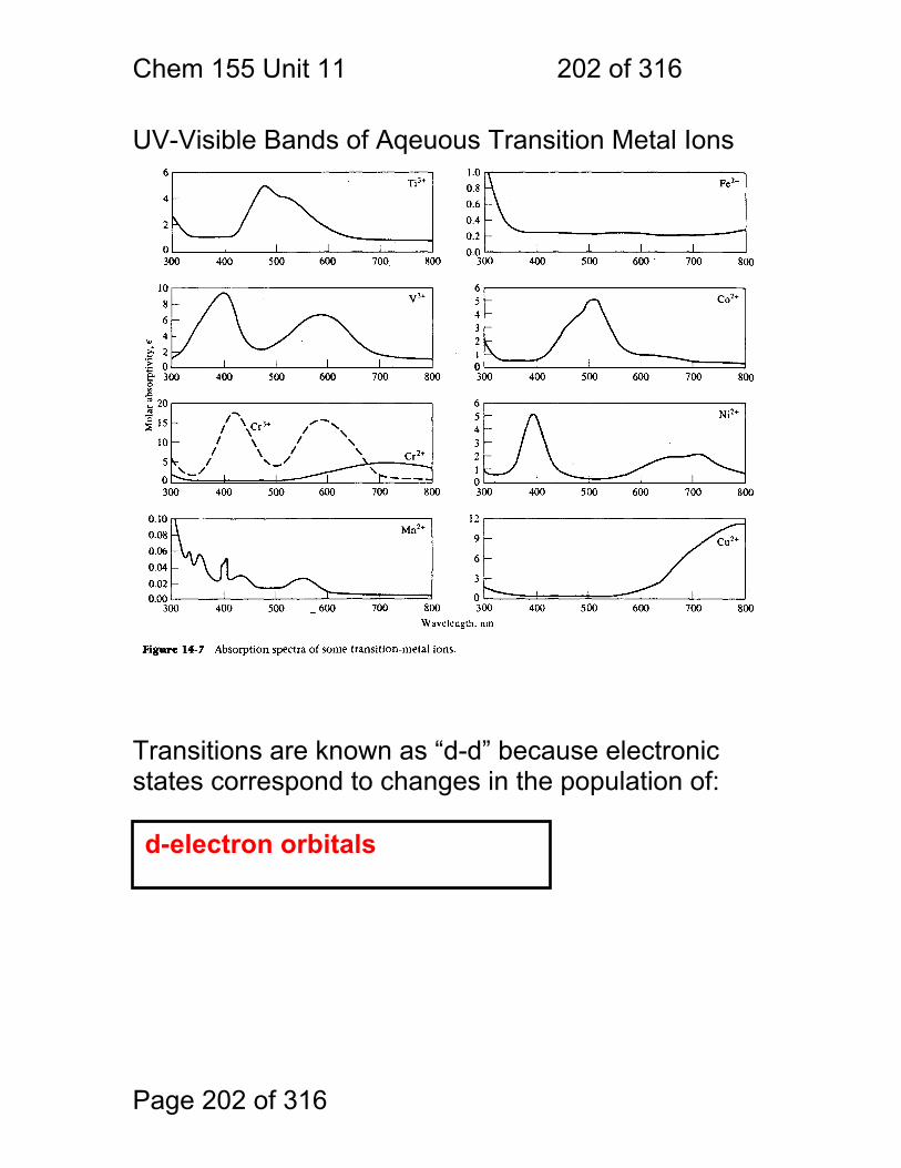
Chem 155 Unit 11 202 of 316
Page 202 of 316
UV-Visible Bands of Aqeuous Transition Metal Ions Transitions are known as “d-d” because electronic states correspond to changes in the population of: d-electron orbitals
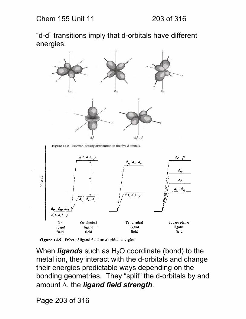
Chem 155 Unit 11 203 of 316
Page 203 of 316
“d-d” transitions imply that d-orbitals have different energies.
When ligands such as H2O coordinate (bond) to the metal ion, they interact with the d-orbitals and change their energies predictable ways depending on the bonding geometries. They “split” the d-orbitals by and amount Δ, the ligand field strength.
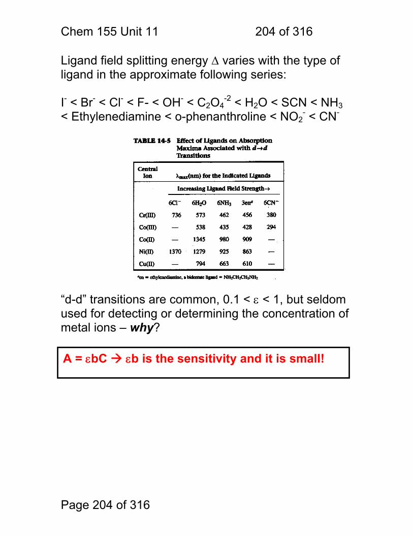
Chem 155 Unit 11 204 of 316
Page 204 of 316
Ligand field splitting energy Δ varies with the type of ligand in the approximate following series: I- < Br- < Cl- < F- < OH- < C2O4
-2 < H2O < SCN < NH3 < Ethylenediamine < o-phenanthroline < NO2
- < CN-
“d-d” transitions are common, 0.1 < ε < 1, but seldom used for detecting or determining the concentration of metal ions – why? A = εbC εb is the sensitivity and it is small!
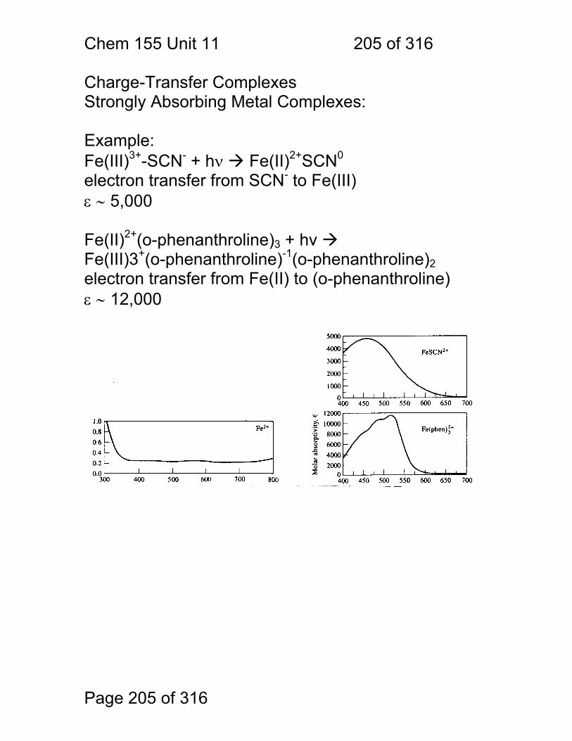
Chem 155 Unit 11 205 of 316
Page 205 of 316
Charge-Transfer Complexes Strongly Absorbing Metal Complexes: Example: Fe(III)3+-SCN- + hν Fe(II)2+SCN0 electron transfer from SCN- to Fe(III) ε ∼ 5,000 Fe(II)2+(o-phenanthroline)3 + hv Fe(III)3+(o-phenanthroline)-1(o-phenanthroline)2 electron transfer from Fe(II) to (o-phenanthroline) ε ∼ 12,000
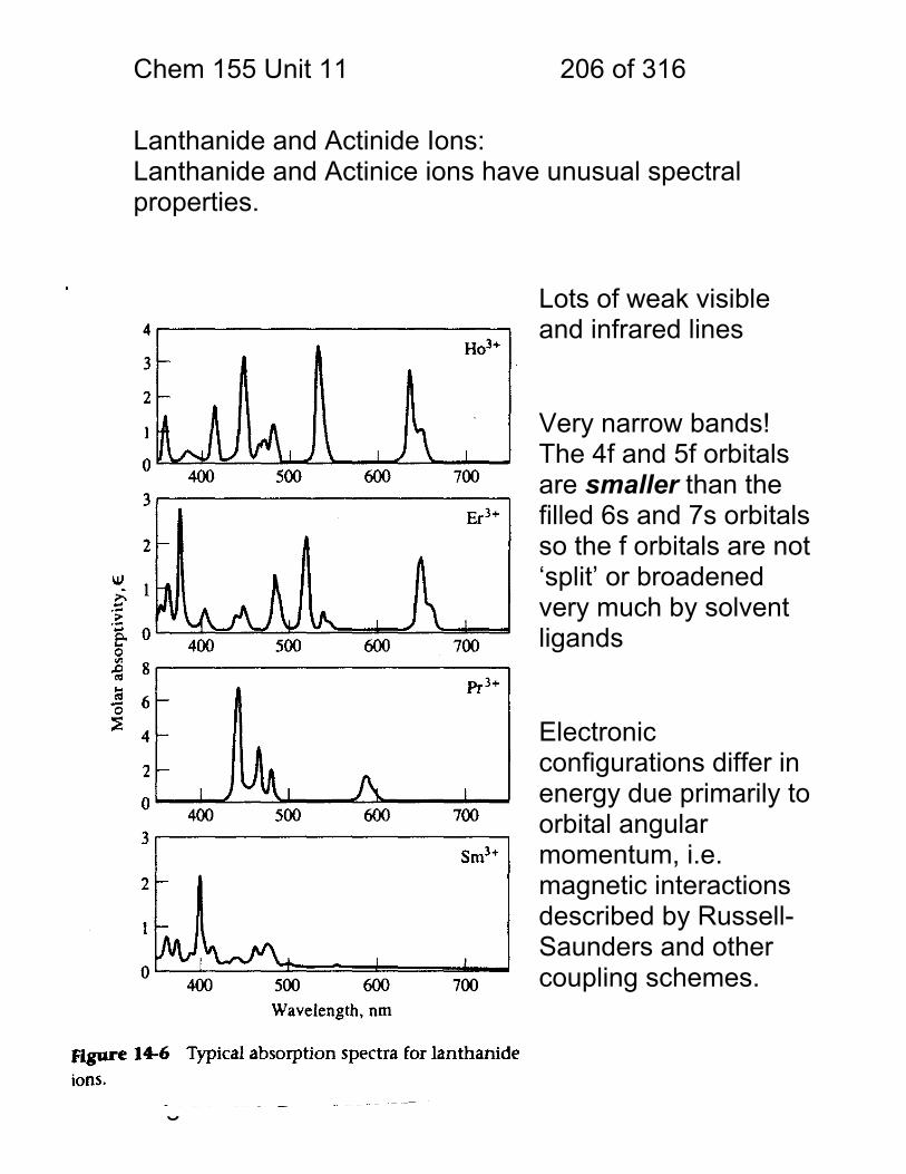
Chem 155 Unit 11 206 of 316
Page 206 of 316
Lanthanide and Actinide Ions: Lanthanide and Actinice ions have unusual spectral properties.
• Lots of weak visible and infrared lines
• Very narrow bands!
The 4f and 5f orbitals are smaller than the filled 6s and 7s orbitals so the f orbitals are not ‘split’ or broadened very much by solvent ligands
• Electronic
configurations differ in energy due primarily to orbital angular momentum, i.e. magnetic interactions described by Russell-Saunders and other coupling schemes.
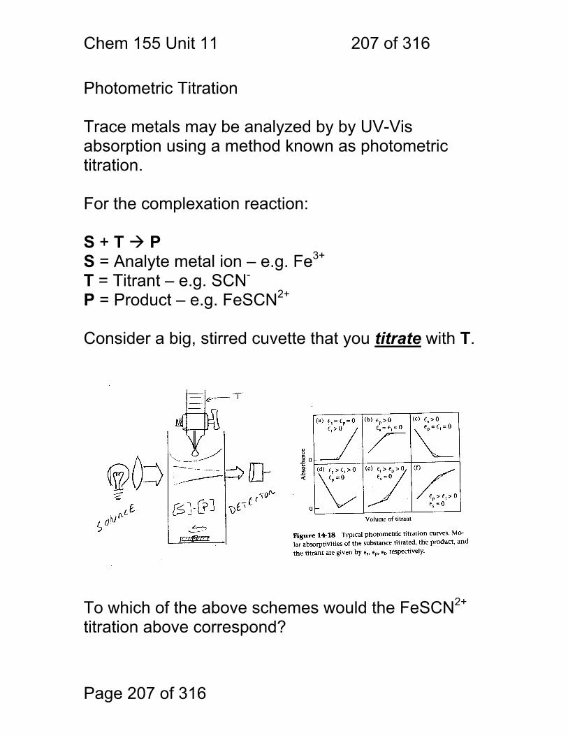
Chem 155 Unit 11 207 of 316
Page 207 of 316
Photometric Titration Trace metals may be analyzed by by UV-Vis absorption using a method known as photometric titration. For the complexation reaction: S + T P S = Analyte metal ion – e.g. Fe3+
T = Titrant – e.g. SCN- P = Product – e.g. FeSCN2+ Consider a big, stirred cuvette that you titrate with T. To which of the above schemes would the FeSCN2+ titration above correspond?
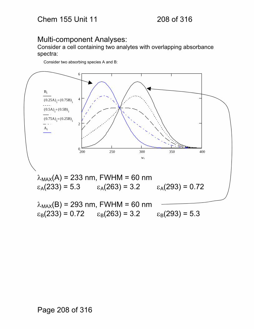
Chem 155 Unit 11 208 of 316
Page 208 of 316
Multi-component Analyses: Consider a cell containing two analytes with overlapping absorbance spectra:
λMAX(A) = 233 nm, FWHM = 60 nm εA(233) = 5.3 εA(263) = 3.2 εA(293) = 0.72 λMAX(B) = 293 nm, FWHM = 60 nm εB(233) = 0.72 εB(263) = 3.2 εB(293) = 5.3
Consider two absorbing species A and B:
200 250 300 350 4000
2
4
6
Bi
0.25A( )i 0.75B( )i+
0.5A( )i 0.5B( )i+
0.75A( )i 0.25B( )i+
Ai
wi
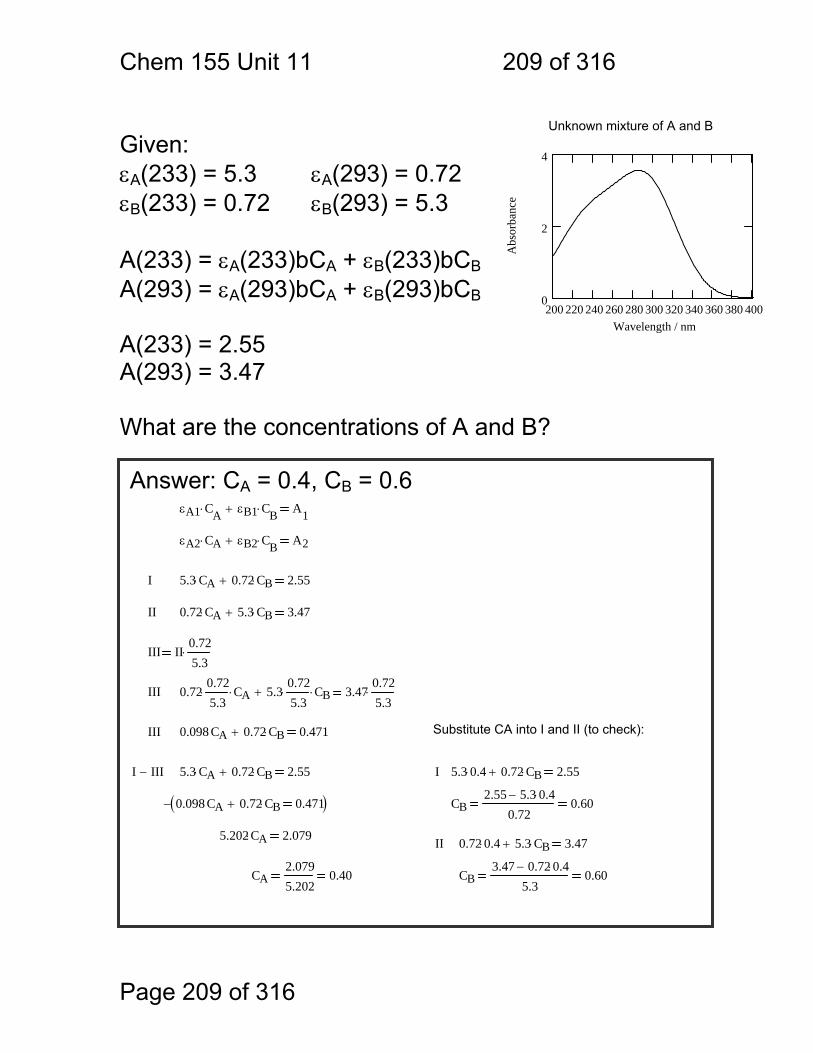
Chem 155 Unit 11 209 of 316
Page 209 of 316
Given: εA(233) = 5.3 εA(293) = 0.72 εB(233) = 0.72 εB(293) = 5.3 A(233) = εA(233)bCA + εB(233)bCB A(293) = εA(293)bCA + εB(293)bCB A(233) = 2.55 A(293) = 3.47 What are the concentrations of A and B?
Answer: CA = 0.4, CB = 0.6
CB3.47 0.72 0.4⋅−
5.30.60CA
2.0795.202
0.40
0.72 0.4⋅ 5.3 CB⋅+ 3.47II5.202 CA⋅ 2.079
CB2.55 5.3 0.4⋅−
0.720.600.098 CA⋅ 0.72 CB⋅+ 0.471( )−
5.3 0.4⋅ 0.72 CB⋅+ 2.55I5.3 CA⋅ 0.72 CB⋅+ 2.55I III−
Substitute CA into I and II (to check):0.098 CA⋅ 0.72 CB⋅+ 0.471III
0.720.725.3
⋅ CA⋅ 5.30.725.3
⋅ CB⋅+ 3.470.725.3
⋅III
III II0.725.3
⋅
0.72 CA⋅ 5.3 CB⋅+ 3.47II
5.3 CA⋅ 0.72 CB⋅+ 2.55I
εA2 CA⋅ εB2 CB⋅+ A2
εA1 CA⋅ εB1 CB⋅+ A1
Unknown mixture of A and B
200 220 240 260 280 300 320 340 360 380 4000
2
4
Wavelength / nm
Abs
orba
nce
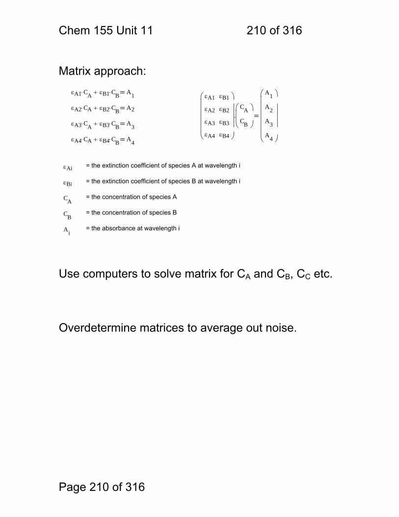
Chem 155 Unit 11 210 of 316
Page 210 of 316
Matrix approach: Use computers to solve matrix for CA and CB, CC etc. Overdetermine matrices to average out noise.
εA1 CA⋅ εB1 CB⋅+ A1
εA2 CA⋅ εB2 CB⋅+ A2
εA1
εA2
εA3
εA4
εB1
εB2
εB3
εB4
⎛⎜⎜⎜⎜⎜⎝
⎞⎟⎟⎟⎟⎟⎠
.CA
CB
⎛⎜⎜⎝
⎞⎟⎟⎠
A1
A2
A3
A4
⎛⎜⎜⎜⎜⎜⎝
⎞⎟⎟⎟⎟⎟⎠
εA3 CA⋅ εB3 CB⋅+ A3
εA4 CA⋅ εB4 CB⋅+ A4
εAi = the extinction coefficient of species A at wavelength i
εBi = the extinction coefficient of species B at wavelength i
CA= the concentration of species A
CB= the concentration of species B
Ai= the absorbance at wavelength i
Chem 155 Unit 12 211 of 316
Page 211 of 316
Intro to Fourier Transform Infrared Spectroscopy Skoog Chapters Covered Fourier Transform Optical Measurements 16A1 Vibrational
Transitions 16A2 Heteronuclear
Diatomics - Classical 16A3 Heteronuclear
Diatomics - Quantum 16A4 Vibrational Modes 16A5 Vibrational Coupling 16C1 Fourier Transform
Instruments
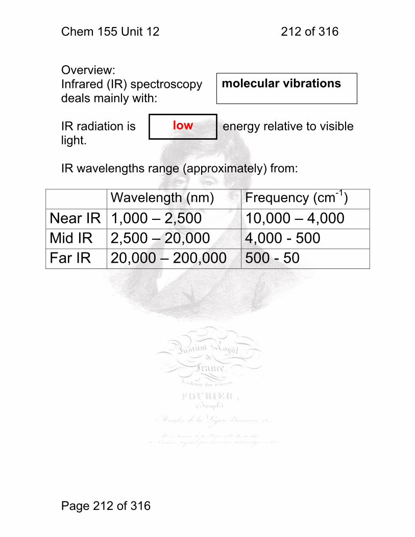
Chem 155 Unit 12 212 of 316
Page 212 of 316
molecular vibrations
Overview: Infrared (IR) spectroscopy deals mainly with: IR radiation is energy relative to visible light. IR wavelengths range (approximately) from:
Wavelength (nm) Frequency (cm-1) Near IR 1,000 – 2,500 10,000 – 4,000 Mid IR 2,500 – 20,000 4,000 - 500 Far IR 20,000 – 200,000 500 - 50
low
Chem 155 Unit 12 213 of 316
Page 213 of 316
Vibrational frequencies (spectra) are sensitive to intermolecular interactions – so one can identify phenomena such as hydrogen bonding, trans or gauche interactions that may control reactivity of molecules.
Why is IR spectroscopy important? 1. UV-Vis spectra are useful, but: all molecules: So most all molecules have:
And most vibrational modes absorb:
So IR spectroscopy is a very general and sensitive analytical tool. 2. Vibrational spectra have a lot of information:
a. Fingerprinting / Identification
b. Quantitation
c. Measurement of Interactions / Configurations
Vibrate
Vibrational absorption spectra
Strongly
Each molecule has a complex but unique signature.
Beer’s law holds for vibrational absorption too!
Chem 155 Unit 12 214 of 316
Page 214 of 316
Some examples of IR spectroscopy • Identification of organic molecules
• Identification of functional groups
• Elucidation of molecular structure
• Elucidation of intermolecular interactions
Routine uses of IR spectroscopy • Confirmation of functional groups
• Confirmation of molecule identity
• Monitoring of atmospheric pollutants.
• Some ‘breathalizers’ use IR absorption of ethanol.
• Quantitation of amide nitrogen for the determination
of protein content in food and other materials.
IR Spectroscopy applications will follow in a later lecture section.
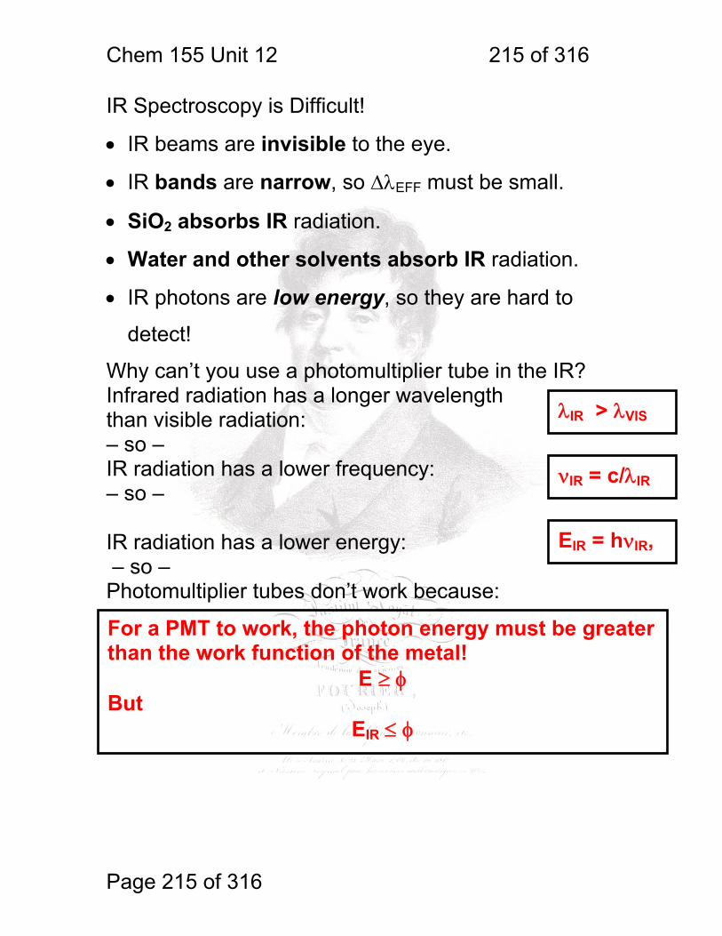
Chem 155 Unit 12 215 of 316
Page 215 of 316
IR Spectroscopy is Difficult! • IR beams are invisible to the eye.
• IR bands are narrow, so ΔλEFF must be small.
• SiO2 absorbs IR radiation.
• Water and other solvents absorb IR radiation.
• IR photons are low energy, so they are hard to
detect!
Why can’t you use a photomultiplier tube in the IR? Infrared radiation has a longer wavelength than visible radiation: – so – IR radiation has a lower frequency: – so – IR radiation has a lower energy: – so – Photomultiplier tubes don’t work because:
λIR > λVIS
νIR = c/λIR
EIR = hνIR,
For a PMT to work, the photon energy must be greater than the work function of the metal!
E ≥ φ But
EIR ≤ φ
Chem 155 Unit 12 216 of 316
Page 216 of 316
Interferometry
time!
slow noisy
Monochromators Are Rarely Used in IR Because: • IR sources are somewhat weak and • IR radiation is somewhat hard to detect, and • IR radiation is hard to focus and • IR spectroscopy must be done at very low effective
bandwidth, Grating or prism-monochromator based IR spectrometers are usually: What is done instead? In interferometry all light frequencies strike the detector at once and the information comes from signal oscillation as a function of: Could you measure the frequency of light by measuring the time between maxima in the electric field?
c 3 108⋅ m⋅ s 1−
⋅:= λ 10 10 6−⋅ m⋅:=
λ
c3.333 10 14−
× s=
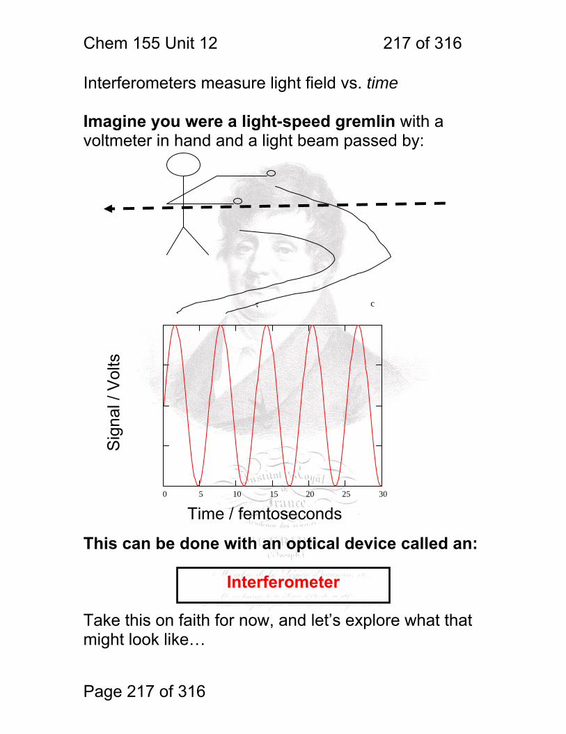
Chem 155 Unit 12 217 of 316
Page 217 of 316
Interferometer
Interferometers measure light field vs. time Imagine you were a light-speed gremlin with a voltmeter in hand and a light beam passed by:
This can be done with an optical device called an: Take this on faith for now, and let’s explore what that might look like…
τ c
0 5 10 15 20 25 30
Sig
nal /
Vol
ts
Time / femtoseconds
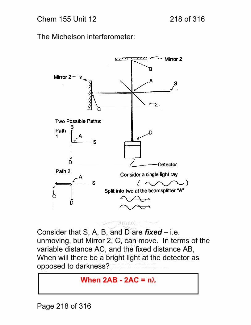
Chem 155 Unit 12 218 of 316
Page 218 of 316
The Michelson interferometer: Consider that S, A, B, and D are fixed – i.e. unmoving, but Mirror 2, C, can move. In terms of the variable distance AC, and the fixed distance AB, When will there be a bright light at the detector as opposed to darkness?
When 2AB - 2AC = nλ
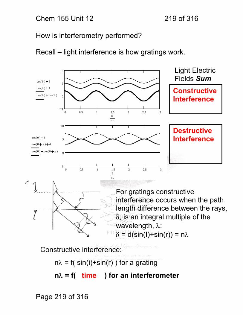
Chem 155 Unit 12 219 of 316
Page 219 of 316
Destructive Interference
How is interferometry performed? Recall – light interference is how gratings work.
cos θ( ) 6
cos θ( ) 4
cos θ( ) cos θ( )
θ
2 π.
0 0.5 1 1.5 2 2.5 35
0
5
10
cos θ( ) 6
cos θ π( ) 4
cos θ( ) cos θ π( )
θ
2 π.
0 0.5 1 1.5 2 2.5 35
0
5
10
Light Electric Fields Sum
For gratings constructive interference occurs when the path length difference between the rays, δ, is an integral multiple of the wavelength, λ: δ = d(sin(I)+sin(r)) = nλ
Constructive interference:
nλ = f( sin(i)+sin(r) ) for a grating
nλ = f( time ) for an interferometer
Constructive Interference
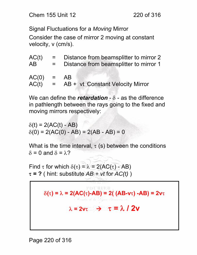
Chem 155 Unit 12 220 of 316
Page 220 of 316
Signal Fluctuations for a Moving Mirror Consider the case of mirror 2 moving at constant velocity, v (cm/s). AC(t) = Distance from beamsplitter to mirror 2 AB = Distance from beamsplitter to mirror 1 AC(0) = AB AC(t) = AB + vt Constant Velocity Mirror We can define the retardation - δ - as the difference in pathlength between the rays going to the fixed and moving mirrors respectively: δ(t) = 2(AC(t) - AB) δ(0) = 2(AC(0) - AB) = 2(AB - AB) = 0 What is the time interval, τ (s) between the conditions δ = 0 and δ = λ? Find τ for which δ(τ) = λ = 2(AC(τ) - AB) τ = ? ( hint: substitute AB + vt for AC(t) )
δ(τ) = λ = 2(AC(τ)-AB) = 2( (AB-vτ) -AB) = 2vτ
λ = 2vτ τ = λ / 2v
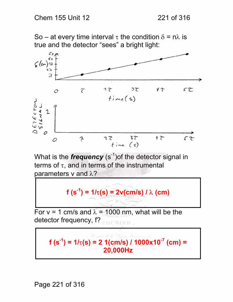
Chem 155 Unit 12 221 of 316
Page 221 of 316
So – at every time interval τ the condition δ = nλ is true and the detector “sees” a bright light:
What is the frequency (s-1)of the detector signal in terms of τ, and in terms of the instrumental parameters v and λ?
For v = 1 cm/s and λ = 1000 nm, what will be the detector frequency, f?
f (s-1) = 1/τ(s) = 2v(cm/s) / λ (cm)
f (s-1) = 1/τ(s) = 2 1(cm/s) / 1000x10-7 (cm) =
20,000Hz
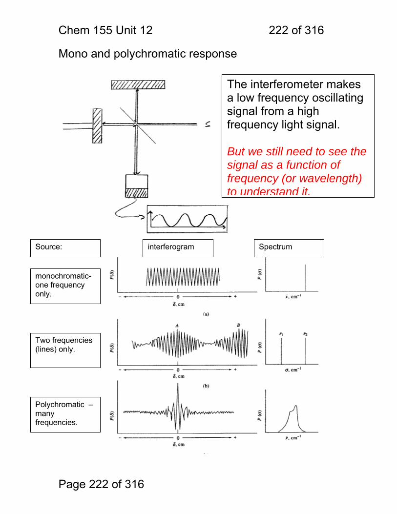
Chem 155 Unit 12 222 of 316
Page 222 of 316
Mono and polychromatic response
The interferometer makes a low frequency oscillating signal from a high frequency light signal. But we still need to see the signal as a function of frequency (or wavelength) to understand it.
monochromatic- one frequency only.
Two frequencies (lines) only.
Polychromatic – many frequencies.
Source: interferogram Spectrum
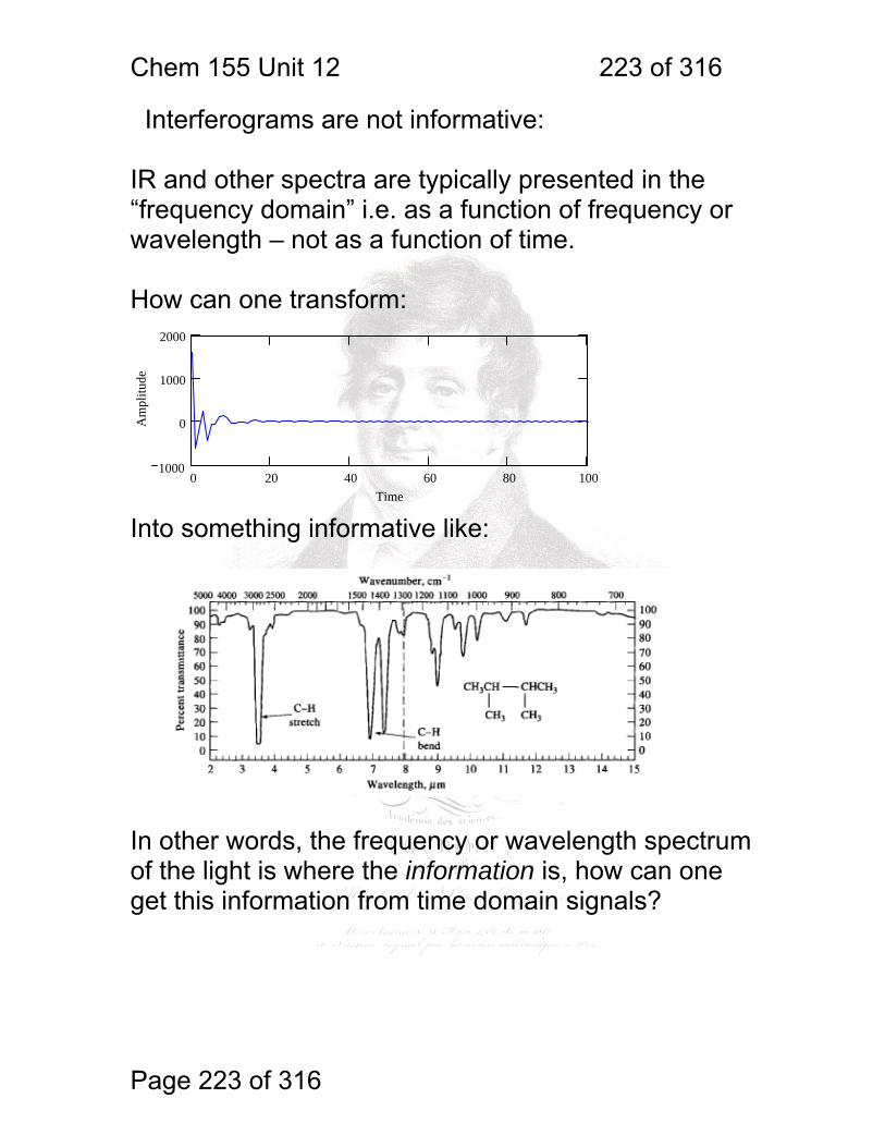
Chem 155 Unit 12 223 of 316
Page 223 of 316
Interferograms are not informative: IR and other spectra are typically presented in the “frequency domain” i.e. as a function of frequency or wavelength – not as a function of time. How can one transform:
Into something informative like:
In other words, the frequency or wavelength spectrum of the light is where the information is, how can one get this information from time domain signals?
0 20 40 60 80 1001000
0
1000
2000
Time
Am
plitu
de
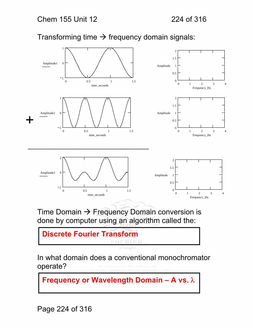
Chem 155 Unit 12 224 of 316
Page 224 of 316
Discrete Fourier Transform
Frequency or Wavelength Domain – A vs. λ
Transforming time frequency domain signals:
Time Domain Frequency Domain conversion is done by computer using an algorithm called the:
In what domain does a conventional monochromator operate?
Amplitude1
time_seconds0 0.5 1 1.5
1
0
1
Amplitude
Frequency_Hz0 1 2 3 4
0
0.5
1
1.5
2
Amplitude2
time_seconds0 0.5 1 1.5
1
0
1
Amplitude
Frequency_Hz0 1 2 3 4
0
0.5
1
1.5
2
+
------------------------------------------------------------------------------------------
Amplitude3
time_seconds0 0.5 1 1.5
2
0
2
Amplitude
Frequency_Hz0 1 2 3 4
0
0.5
1
1.5
2
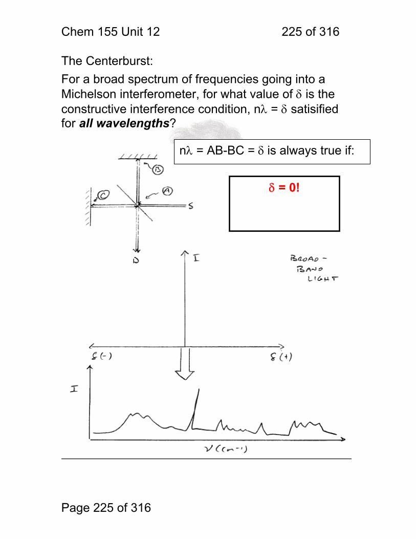
Chem 155 Unit 12 225 of 316
Page 225 of 316
The Centerburst: For a broad spectrum of frequencies going into a Michelson interferometer, for what value of δ is the constructive interference condition, nλ = δ satisified for all wavelengths?
δ = 0!
nλ = AB-BC = δ is always true if:
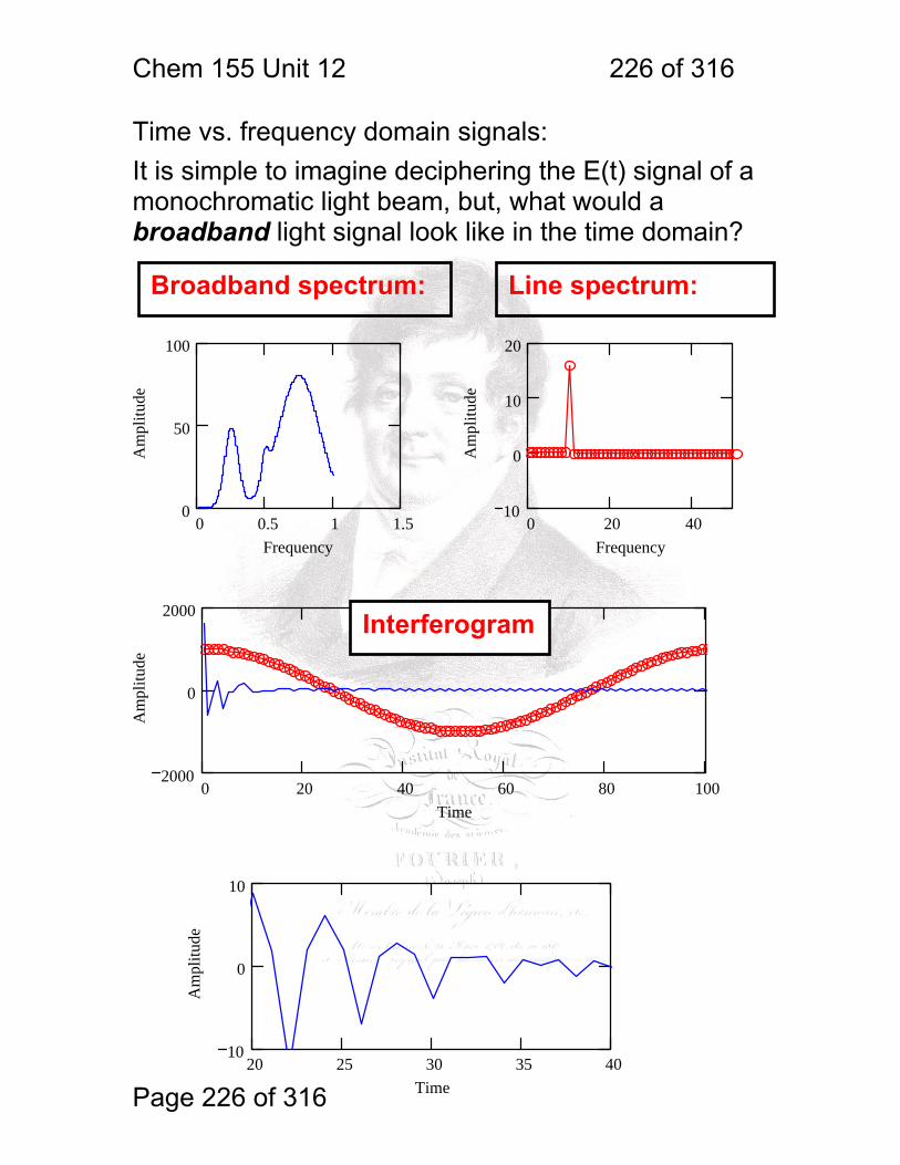
Chem 155 Unit 12 226 of 316
Page 226 of 316
Time vs. frequency domain signals: It is simple to imagine deciphering the E(t) signal of a monochromatic light beam, but, what would a broadband light signal look like in the time domain?
Broadband spectrum: Line spectrum:
0 0.5 1 1.50
50
100
Frequency
Am
plitu
de
0 20 4010
0
10
20
Frequency
Am
plitu
de
0 20 40 60 80 1002000
0
2000
Time
Am
plitu
de
20 25 30 35 4010
0
10
Time
Am
plitu
de
Interferogram
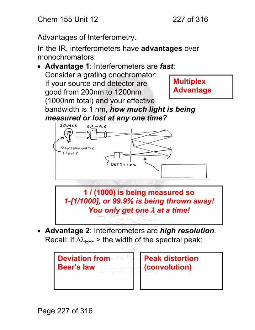
Chem 155 Unit 12 227 of 316
Page 227 of 316
1 / (1000) is being measured so 1-[1/1000], or 99.9% is being thrown away!
You only get one λ at a time!
Deviation from Beer’s law
Peak distortion (convolution)
Multiplex Advantage
Advantages of Interferometry. In the IR, interferometers have advantages over monochromators: • Advantage 1: Interferometers are fast:
Consider a grating onochromator: If your source and detector are good from 200nm to 1200nm (1000nm total) and your effective bandwidth is 1 nm, how much light is being measured or lost at any one time?
• Advantage 2: Interferometers are high resolution.
Recall: If ΔλEFF > the width of the spectral peak:
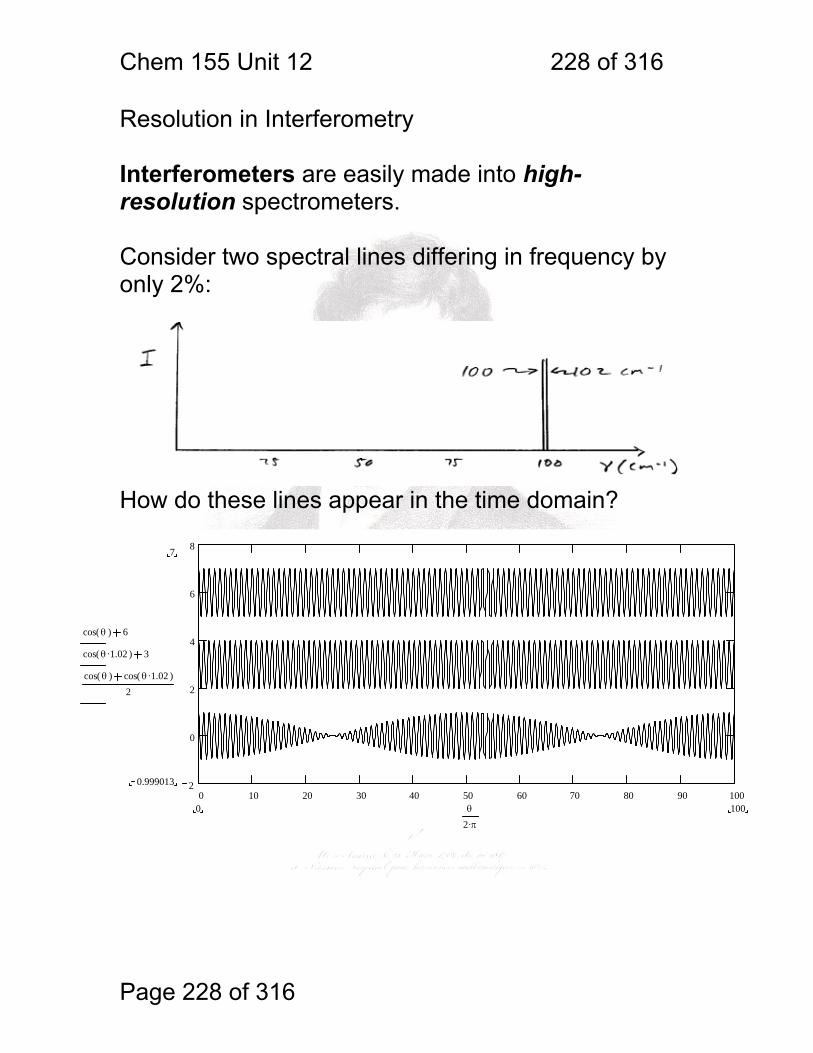
Chem 155 Unit 12 228 of 316
Page 228 of 316
Resolution in Interferometry Interferometers are easily made into high-resolution spectrometers. Consider two spectral lines differing in frequency by only 2%:
How do these lines appear in the time domain?
7
0.999013
cos θ( ) 6
cos θ 1.02.( ) 3
cos θ( ) cos θ 1.02.( )2
1000 θ
2 π.
0 10 20 30 40 50 60 70 80 90 1002
0
2
4
6
8
Chem 155 Unit 12 229 of 316
Page 229 of 316
Let us define resolution as: Δν = ν1 - ν2 when ν1 can just be separated from ν2. I assert that to separate, or resolve these lines in the frequency domain spectrum, we must scan the retardation, δ, from 0 (where ν1 and ν2 are in phase) to a new value, let’s just call it “δ” where the two signals are again in phase. The frequency of oscillation of the signal in time is:
f = 2v(cm/s) / λ(cm) = 2 v ν where ν is the light frequency in wavenumbers (cm-1). The light power function will be sinusoidal: P(δ) = Pi cos(2 π f t) = Pi cos(2 π (2vν) t) If we substitute v, the mirror velocity, with δ/2t = v we get intensity versus retardation: P(δ) = B cos(2 π δ ν)
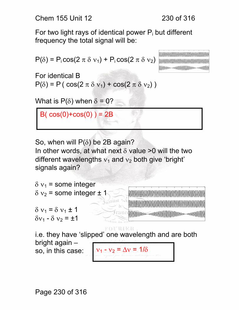
Chem 155 Unit 12 230 of 316
Page 230 of 316
ν1 - ν2 = Δν = 1/δ
For two light rays of identical power Pi but different frequency the total signal will be: P(δ) = Pi cos(2 π δ ν1) + Pi cos(2 π δ ν2) For identical B P(δ) = P ( cos(2 π δ ν1) + cos(2 π δ ν2) ) What is P(δ) when δ = 0?
So, when will P(δ) be 2B again? In other words, at what next δ value >0 will the two different wavelengths ν1 and ν2 both give ‘bright’ signals again? δ ν1 = some integer δ ν2 = some integer ± 1 δ ν1 = δ ν1 ± 1 δν1 - δ ν2 = ±1 i.e. they have ‘slipped’ one wavelength and are both bright again – so, in this case:
B( cos(0)+cos(0) ) = 2B
Chem 155 Unit 12 231 of 316
Page 231 of 316
For a large δ, Δν is small and resolution is high! Consider an interferometer with a mirror travel d = 0.5 cm that is operating in the mid visible at 500 nm: ν = 107/500 nm = 20,000 cm-1 δ = 2d = 1 cm Δν = 1/δ = 1/1cm, so 20,001 cm-1 can be resolved from 20,000 cm-1. 107 / 20,001 cm-1 = 499.975 nm. So, 500 nm can be resolved from 499.975 nm. Δλ = 500 - 499.765 = 0.025nm ΔλEFF = 0.025nm is very difficult to achieve with a monochromator! Remember that δ is equal to 2d – twice the mirror displacement.
Chem 155 Unit 12 232 of 316
Page 232 of 316
Conclusions and Questions: Infrared spectroscopy is important because:
1. Virtually all molecules have a unique vibrational spectroscopic signature in the infrared.
2. Most molecules absorb strongly! So IR can be quite sensitive for both identification and quantitation.
3. But IR radiation is harder to manage with a monochromator because sources are weak, detectors are less sensitive and high resolution is often needed.
4. So interferometry is done instead, which is both inherently fast and high reseolution.
Interferometry converts optical frequency directly into a frequency on the detector:
1. What frequency would a 3000 cm-1 source produce in an interferometer operating with a mirror velocity of 1 cm/s?
2. If the mirror travel were 1 cm, what would be the resolution (ΔλEFF) in cm-1?
3. What will this value be in nm? 4. What focal length would be needed with a
monochromator with a 1000 nm grating spacing and slits at 0.4 mm?
Chem 155 Unit 12 233 of 316
Page 233 of 316
Answers:
The detector frequency would be 6 kHz – not a problem. The effective bandwidth for a 1 cm drive is 0.5 cm-1. At 3000 cm-1 – this equates to 0.55 nm. The minimum focal length required to achieve this bandwidth with a monochromator would be 0.5 m, a fairly large system, especially when compared to a 1 cm interferometer drive.
f 2 v⋅ ν⋅ 2 1⋅cms
⋅ 3000⋅ cm 1−⋅ 6000s-1
=
effective bandwidth in cm 1− : ΔνEFF1δ
12 d⋅
12 1⋅ cm⋅
0.5cm 1−=
107 nmcm
⋅
3000 cm 1−⋅( )
107 nmcm
⋅
3000.5cm 1−⋅
− 0.555nm=effective bandwidth in nm:
ΔλEFFw d⋅ cos r( )⋅
n F⋅F
w d⋅ cos r( )⋅
n ΔλEFF⋅
0.4 mm⋅ 1000⋅ nm⋅ cos 45π
180⋅⎛⎜
⎝⎞⎟⎠
⋅
1 0.55⋅ nm⋅0.514m=
Chem 155 Unit 13 Page 234 of 316
Page 234 of 316
Infrared Spectrometry: Selection Rules, Normal Modes and Group Frequencies Skoog Chapters Covered: 16A all, 16B – Sources and Transducers 16C-1, FT-Instruments Rough overview of the optical spectroscopy ranges:
λ (nm) ν (cm-1) T (K) Designation Phenomena 100 100,000 140,000 UV σ-σ*, n-σ*,
n-π*, π-π* Valence electron excitation
VIS
1,000 10,000 14,000 Near IR low-E electronic Hi-E vibrations OH, C≡O, NH
Mid IR Group Frequencies
10,000 1,000 1,400 Fingerprint Inorganics, High-Z, Low-k Lattice vibration, Pure rotations
Far IR μ-wave 100,000 100 140
1,000,000 10 14
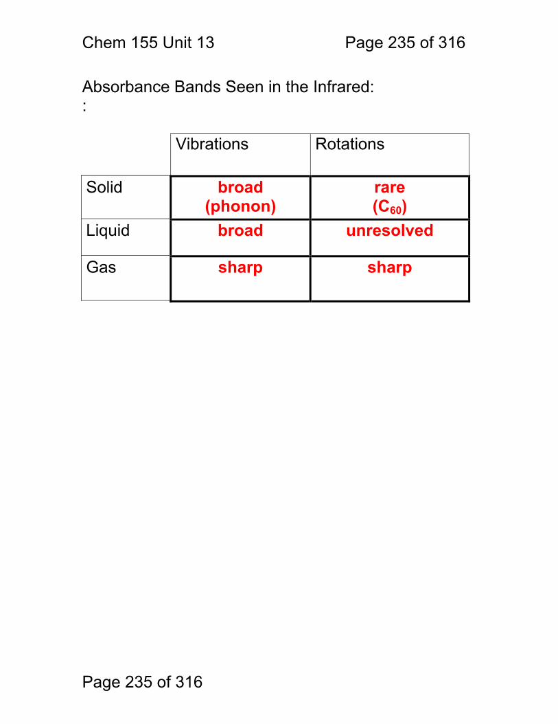
Chem 155 Unit 13 Page 235 of 316
Page 235 of 316
Absorbance Bands Seen in the Infrared: : Vibrations Rotations
Solid broad (phonon)
rare (C60)
Liquid broad unresolved
Gas sharp sharp

Chem 155 Unit 13 Page 236 of 316
Page 236 of 316
IR Selection Rules How does electromagnetic radiation make a molecule vibrate? Consider the diatomic molecule H-Cl.
Electric Field Vector of Light
E θ( )
θ
H
Cl Cl Cl
Force
δ
δ
+
-
In Out In
H H
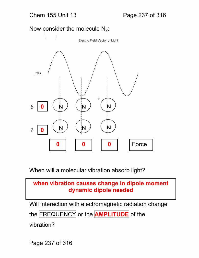
Chem 155 Unit 13 Page 237 of 316
Page 237 of 316
Now consider the molecule N2: When will a molecular vibration absorb light? Will interaction with electromagnetic radiation change
the FREQUENCY or the AMPLITUDE of the
vibration?
when vibration causes change in dipole moment dynamic dipole needed
Electric Field Vector of Light
E θ( )
θ
N
Force
δ
δ
0
0
0 0 0
N
N
N
N
N
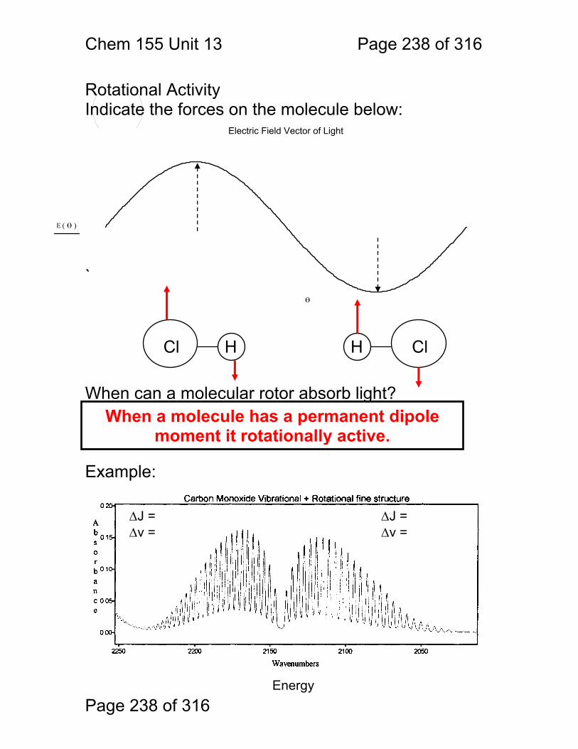
Chem 155 Unit 13 Page 238 of 316
Page 238 of 316
Rotational Activity Indicate the forces on the molecule below:
`
When can a molecular rotor absorb light? Example:
Electric Field Vector of Light
E θ( )
θ
HCl H Cl
When a molecule has a permanent dipole moment it rotationally active.
Energy
ΔJ = Δv =
ΔJ = Δv =
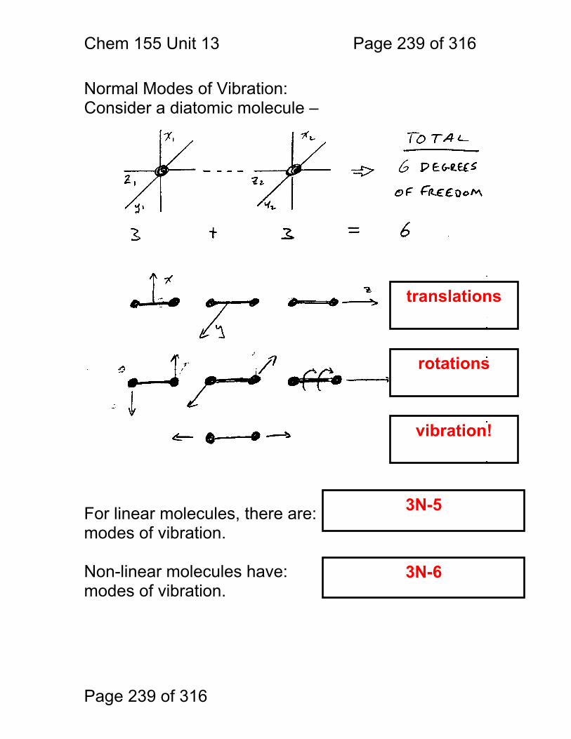
Chem 155 Unit 13 Page 239 of 316
Page 239 of 316
Normal Modes of Vibration: Consider a diatomic molecule – For linear molecules, there are: modes of vibration. Non-linear molecules have: modes of vibration.
translations
rotations
vibration!
3N-5
3N-6
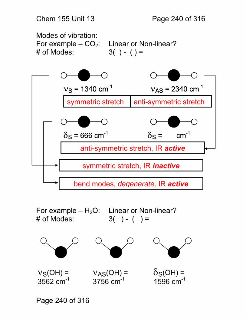
Chem 155 Unit 13 Page 240 of 316
Page 240 of 316
Modes of vibration: For example – CO2: Linear or Non-linear? # of Modes: 3( ) - ( ) = For example – H2O: Linear or Non-linear? # of Modes: 3( ) - ( ) =
νS = 1340 cm-1 νAS = 2340 cm-1
δS = 666 cm-1 δS = cm-1
νS = 1340 cm-1 νAS = 2340 cm-1
δS = 666 cm-1 δS = cm-1
νS(OH) = 3562 cm-1
νAS(OH) = 3756 cm-1
δS(OH) = 1596 cm-1
symmetric stretch anti-symmetric stretch
anti-symmetric stretch, IR active
symmetric stretch, IR inactive
bend modes, degenerate, IR active
Chem 155 Unit 13 Page 241 of 316
Page 241 of 316
1.1.60 One may see more than 3N-5/6 bands: • Overtones:
• Combinations:
1.1.61 One may see fewer than 3N-5/6 bands: • ν not in 400-4000 cm-1 range of typical FTIR
• Band may be weak
• Band may be broad and overlap another band
• Bands may be degenerate
• Bands may be ‘forbidden’, i.e. if there may be no change in dipole moment during the vibrational mode.
Δv = ±2, ±3
νC = νA + νB and νA - νB
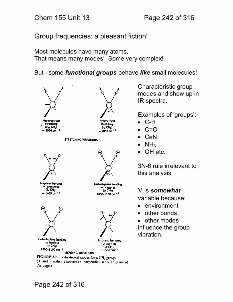
Chem 155 Unit 13 Page 242 of 316
Page 242 of 316
Group frequencies: a pleasant fiction! Most molecules have many atoms. That means many modes! Some very complex! But –some functional groups behave like small molecules!
Characteristic group modes and show up in IR spectra. Examples of ‘groups’: • C-H • C=O • C≡N • NH3 • OH etc. 3N-6 rule irrelevant to this analysis
ν is somewhat variable because: • environment • other bonds • other modes influence the group vibration.
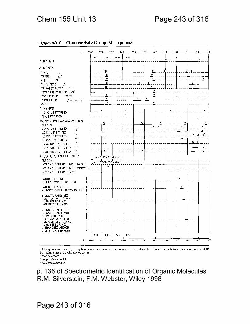
Chem 155 Unit 13 Page 243 of 316
Page 243 of 316
p. 136 of Spectrometric Identification of Organic Molecules R.M. Silverstein, F.M. Webster, Wiley 1998
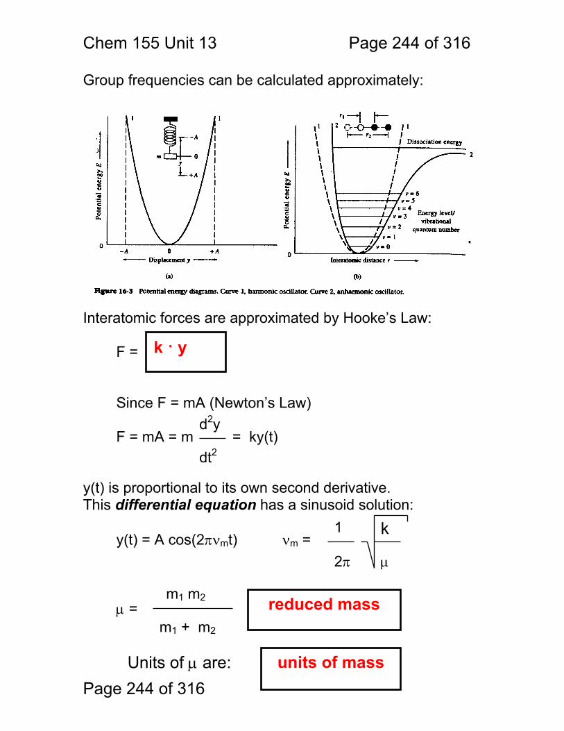
Chem 155 Unit 13 Page 244 of 316
Page 244 of 316
Group frequencies can be calculated approximately: Interatomic forces are approximated by Hooke’s Law:
F = Since F = mA (Newton’s Law) F = mA = m = ky(t) y(t) is proportional to its own second derivative. This differential equation has a sinusoid solution: y(t) = A cos(2πνmt) νm = μ =
k · y
d2y
dt2
1
2π
k
μ
m1 m2
m1 + m2 reduced mass
Units of μ are: units of mass
Chem 155 Unit 13 Page 245 of 316
Page 245 of 316
Classical calculations (above) tell you the natural frequency of a classical oscillator. Quantuum mechanical calculations tell you the allowed energy levels (E). From Planck and Einstein’s equation E=hν we can calculate the light frequencies (ν). E = (v + ½ )h νm
v = vibrational quantuum number = 0,1,2… Δv = 0,±1 = the selection rule for vibrational transitions again: νm = so: ΔE = Δv h νm = ±1 = hν note: νm is the oscillator frequency and ν is the light frequency What is the relationship between ν and νm?
What is the relationship between light frequency, ν, and light wavenumber, ν (cm-1)? (ν = 1/λ(cm)).
1
2π
k
μ
h
2π
k
μ
the light frequency equals the oscillator frequency
ν = cν
Chem 155 Unit 13 Page 246 of 316
Page 246 of 316
Summary:
• Molecules vibrate – their atoms move back and forth relative to each other.
• Vibrations come in certain modes that involve the whole molecule.
• Modes wherein the molecule has a change in dipole moment may be excited by IR radiation.
• The higher the mass, the lower the mode frequency.
• The stronger the bond, the higher the mode frequency.
• In complex molecules with many atoms, some individual parts of the molecule behave as though they were independent.
• The absorption bands corresponding to these group modes are known as group frequencies and allow one to identify functional groups such as aldehydes, amides, olefins etc. on a given molecule.
Chem 155 Unit 14 247 of 316
Page 247 of 316
Nearly everything absorbs IR radiation!
Beam is invisible to the eye – hard to align IR Sources are often weak (blackbodies) Detectors are not very sensitive
optics and solvents will have strong absorption
Infrared Spectrometry - Applications Skoog Chapters Covered 17A1 Sample Handling in Mid-IR 17A2 Group Frequencies 17A3 Quantitation in Mid IR 17B Reflection Methods 17D Near IR applications 17E Far IR applications The major difficulty in infrared spectroscopy is related to the IR selection rule:
Δμ during vibration => IR active
Other difficulties relative to, e.g. visible spectroscopy:
Chem 155 Unit 14 248 of 316
Page 248 of 316
use mirrors instead of lenses
use interferometer instead of monochromator
use high-atomic-mass materials with weak inter atomic bonds – typical materials are: 1. CaF2 2. ZnSe 3. KBr 4. NaCl
use solvents transparent in selected spectral regions
avoid solvents completely
use reflection-absorption instead of transmission
Strategies used to make IR spectrometry work - 1. Poor sources and detectors:
1. Optics absorb IR light:
2. Materials for transmissive optics:
3. Sample Handling:
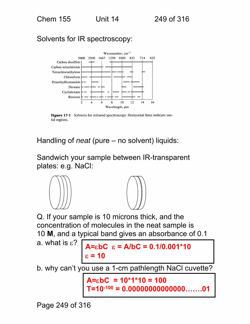
Chem 155 Unit 14 249 of 316
Page 249 of 316
Solvents for IR spectroscopy:
Handling of neat (pure – no solvent) liquids: Sandwich your sample between IR-transparent plates: e.g. NaCl: Q. If your sample is 10 microns thick, and the concentration of molecules in the neat sample is 10 M, and a typical band gives an absorbance of 0.1 a. what is ε? b. why can’t you use a 1-cm pathlength NaCl cuvette?
A=εbC ε = A/bC = 0.1/0.001*10 ε = 10
A=εbC = 10*1*10 = 100 T=10-100 = 0.00000000000000…….01
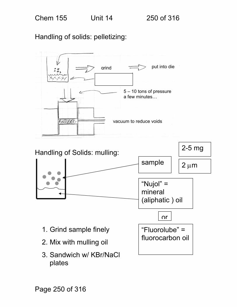
Chem 155 Unit 14 250 of 316
Page 250 of 316
Handling of solids: pelletizing:
grind put into die
5 – 10 tons of pressure a few minutes…
vacuum to reduce voids
Handling of Solids: mulling:
1. Grind sample finely
2. Mix with mulling oil
3. Sandwich w/ KBr/NaCl plates
sample
“Nujol” = mineral (aliphatic ) oil
“Fluorolube” = fluorocarbon oil
2-5 mg
2 μm
or
Chem 155 Unit 14 251 of 316
Page 251 of 316
You use an open beam to approximate Po
Sample plus window plus mulling oil absorbance plus reflection losses.
qualitative
Functional group identification
Spectral ‘fingerprinting’
A general problem with pellets and mulls: A = -log[P/Po] How do you measure Po?
So – the spectra you obtain, are a sum of absorbances – the spectra contain:
IR spectra obtained with these sampling methods are useful for identification, not quantitation:
The two pieces of information that are useful:
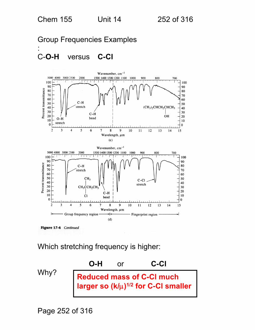
Chem 155 Unit 14 252 of 316
Page 252 of 316
Group Frequencies Examples : C-O-H versus C-Cl Which stretching frequency is higher:
O-H or C-Cl Why? Reduced mass of C-Cl much
larger so (k/μ)1/2 for C-Cl smaller
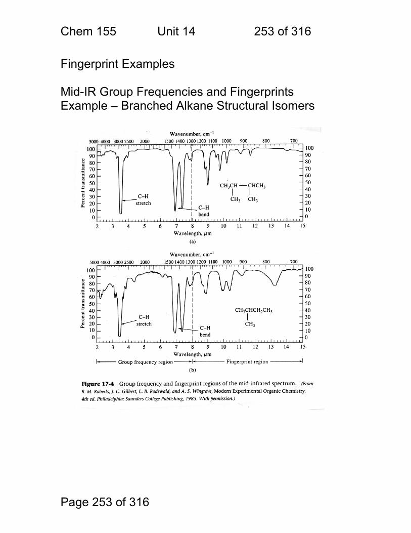
Chem 155 Unit 14 253 of 316
Page 253 of 316
Fingerprint Examples Mid-IR Group Frequencies and Fingerprints Example – Branched Alkane Structural Isomers
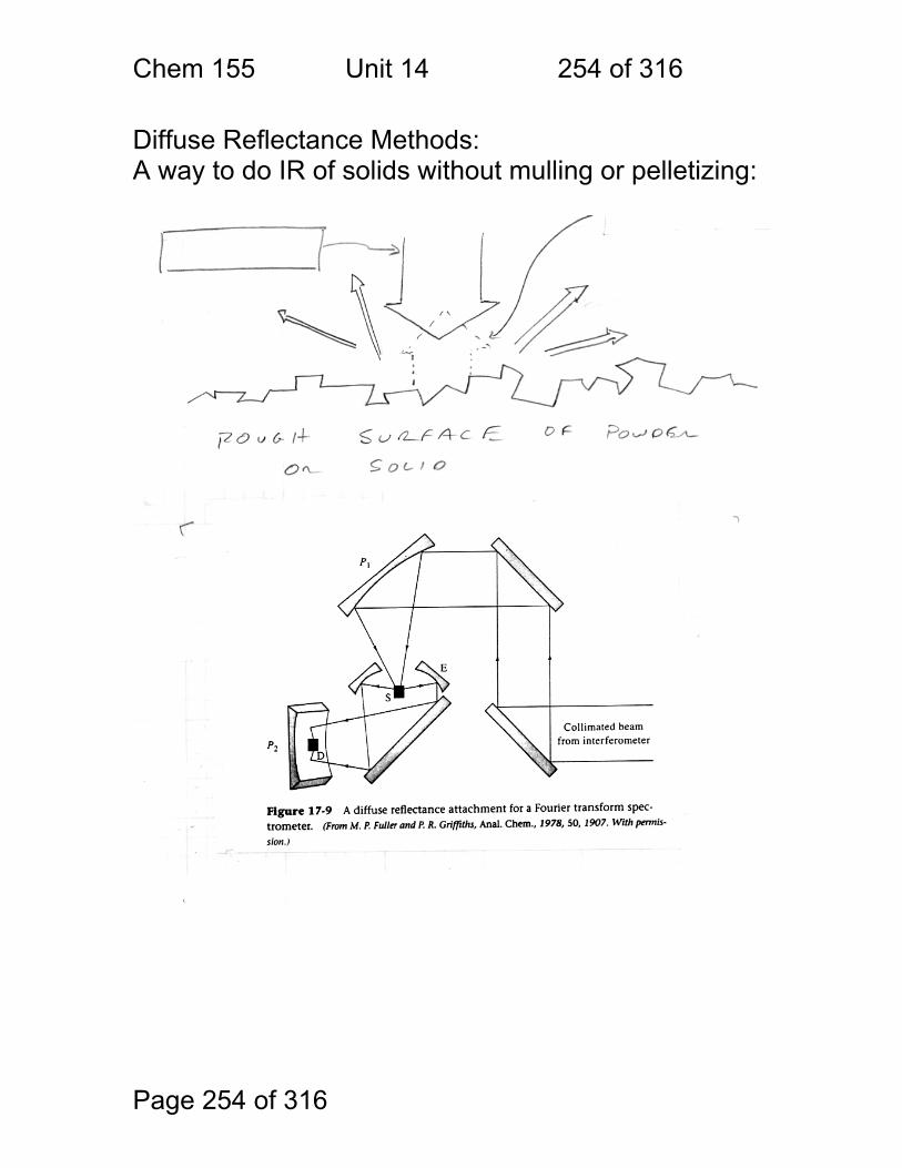
Chem 155 Unit 14 254 of 316
Page 254 of 316
Diffuse Reflectance Methods: A way to do IR of solids without mulling or pelletizing:
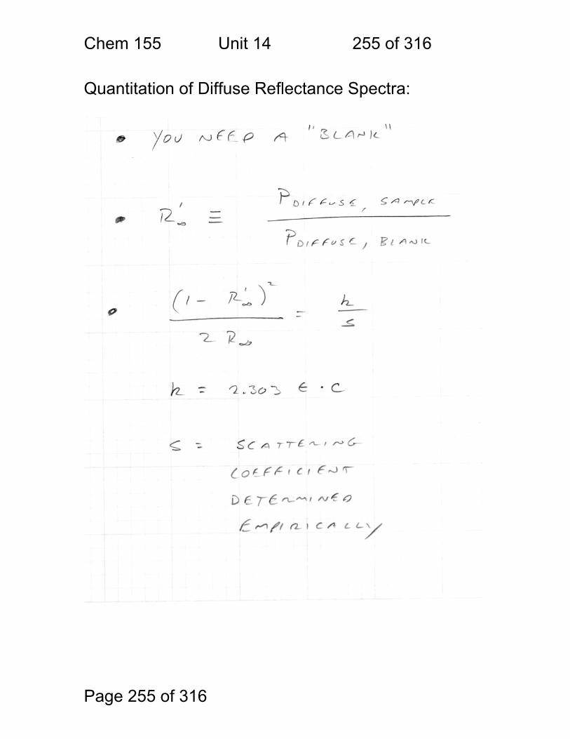
Chem 155 Unit 14 255 of 316
Page 255 of 316
Quantitation of Diffuse Reflectance Spectra:
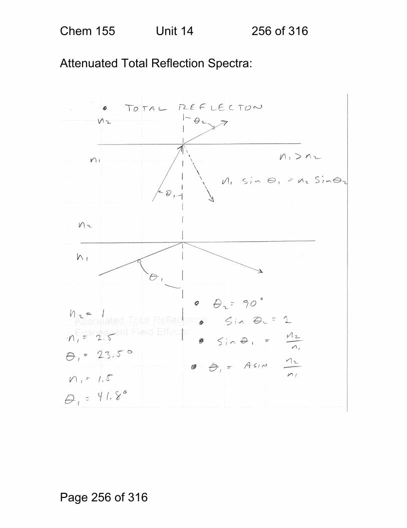
Chem 155 Unit 14 256 of 316
Page 256 of 316
Attenuated Total Reflection Spectra:
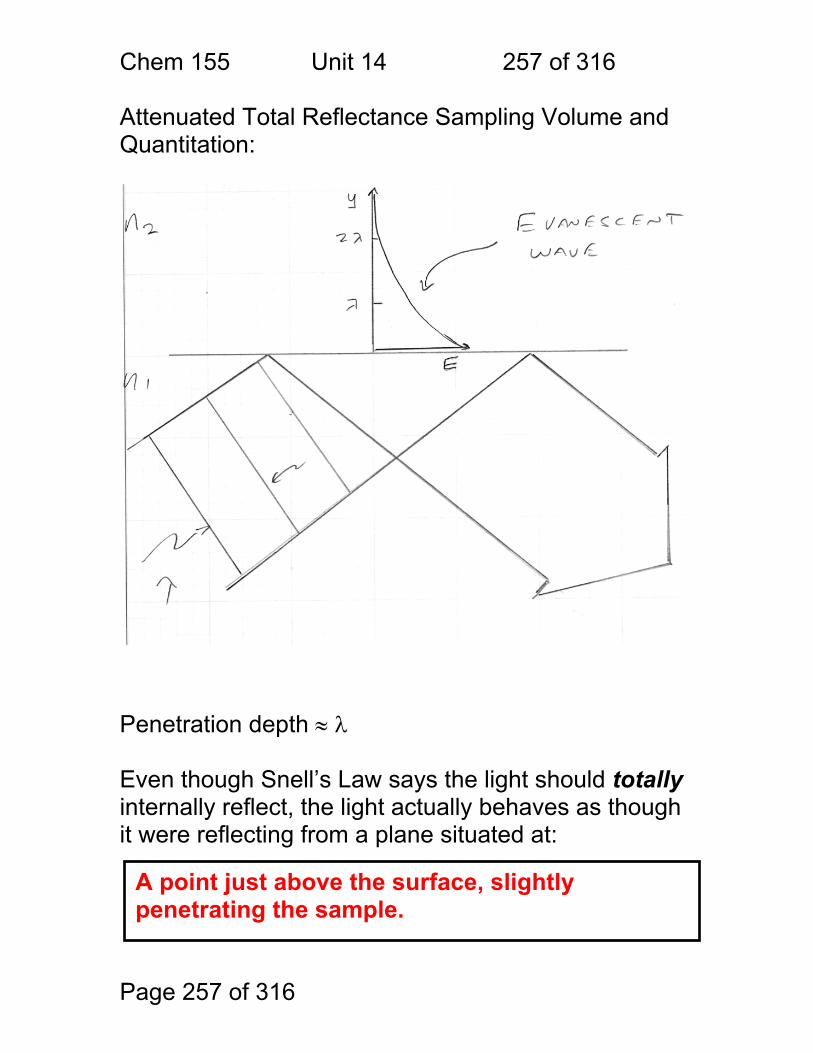
Chem 155 Unit 14 257 of 316
Page 257 of 316
A point just above the surface, slightly penetrating the sample.
Attenuated Total Reflectance Sampling Volume and Quantitation: Penetration depth ≈ λ Even though Snell’s Law says the light should totally internally reflect, the light actually behaves as though it were reflecting from a plane situated at:
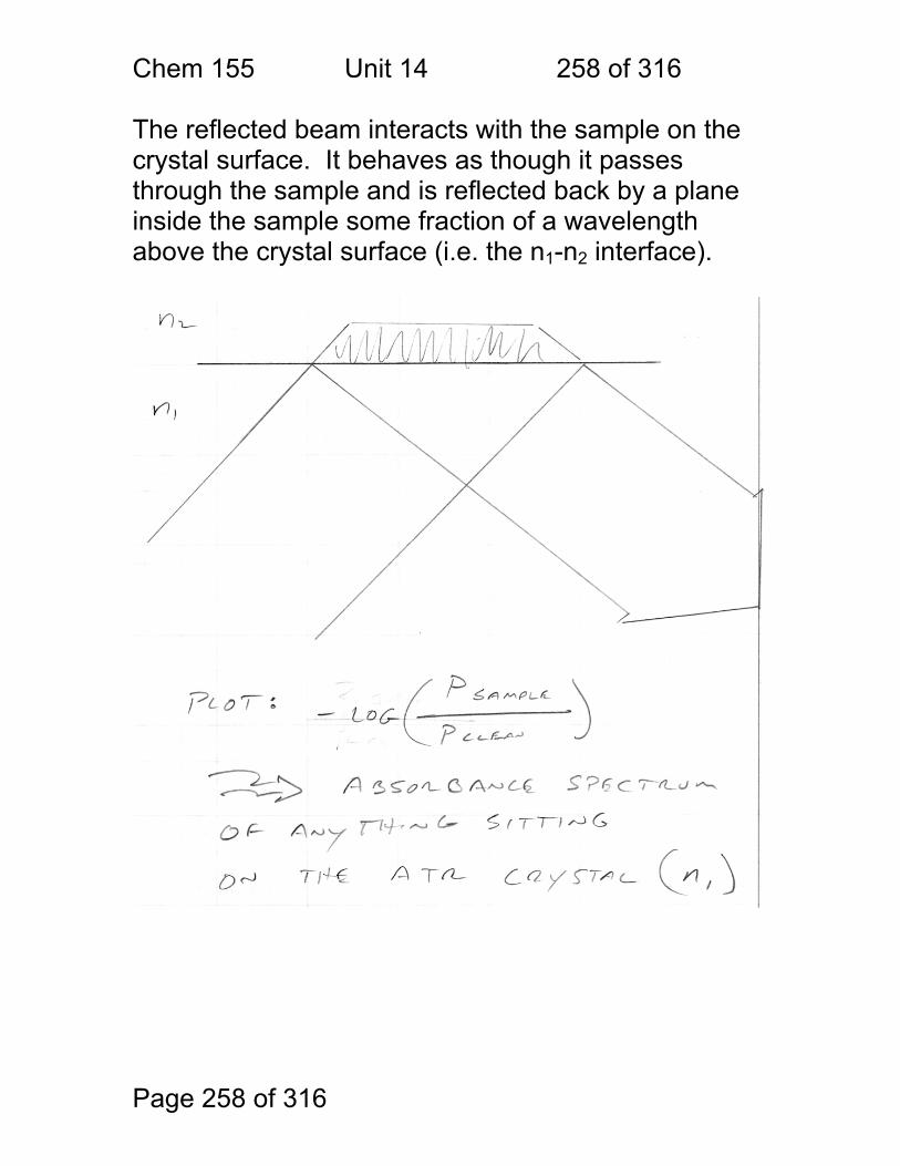
Chem 155 Unit 14 258 of 316
Page 258 of 316
The reflected beam interacts with the sample on the crystal surface. It behaves as though it passes through the sample and is reflected back by a plane inside the sample some fraction of a wavelength above the crystal surface (i.e. the n1-n2 interface).
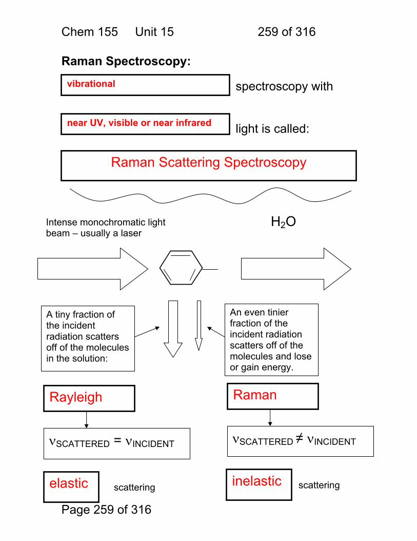
Chem 155 Unit 15 259 of 316
Page 259 of 316
Raman Spectroscopy: spectroscopy with light is called:
vibrational
near UV, visible or near infrared
Raman Scattering Spectroscopy
H2O
A tiny fraction of the incident radiation scatters off of the molecules in the solution:
Intense monochromatic light beam – usually a laser
Rayleigh
νSCATTERED = νINCIDENT
elastic scattering
An even tinier fraction of the incident radiation scatters off of the molecules and lose or gain energy.
Raman
νSCATTERED ≠ νINCIDENT
inelastic scattering
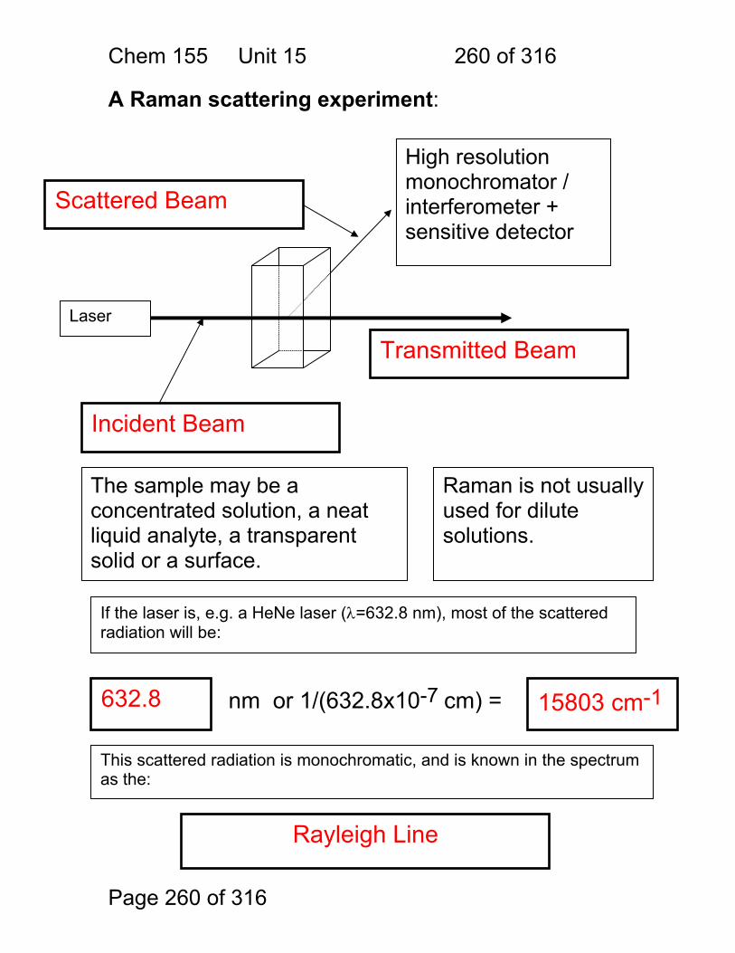
Chem 155 Unit 15 260 of 316
Page 260 of 316
A Raman scattering experiment:
Laser
Scattered Beam
Transmitted Beam
Incident Beam
High resolution monochromator / interferometer + sensitive detector
The sample may be a concentrated solution, a neat liquid analyte, a transparent solid or a surface.
If the laser is, e.g. a HeNe laser (λ=632.8 nm), most of the scattered radiation will be:
Raman is not usually used for dilute solutions.
632.8 15803 cm-1 nm or 1/(632.8x10-7 cm) =
This scattered radiation is monochromatic, and is known in the spectrum as the:
Rayleigh Line
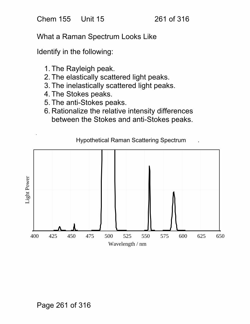
Chem 155 Unit 15 261 of 316
Page 261 of 316
What a Raman Spectrum Looks Like Identify in the following:
1. The Rayleigh peak. 2. The elastically scattered light peaks. 3. The inelastically scattered light peaks. 4. The Stokes peaks. 5. The anti-Stokes peaks. 6. Rationalize the relative intensity differences
between the Stokes and anti-Stokes peaks.
.
400 425 450 475 500 525 550 575 600 625 650Wavelength / nm
Ligh
t Pow
er
Hypothetical Raman Scattering Spectrum .
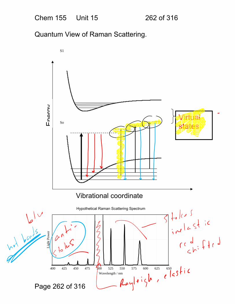
Chem 155 Unit 15 262 of 316
Page 262 of 316
Quantum View of Raman Scattering.
Ene
rgy
So
S1
400 425 450 475 500 525 550 575 600 625 650Wavelength / nm
Ligh
t Pow
er
Hypothetical Raman Scattering Spectrum
Vibrational coordinate
Virtual states
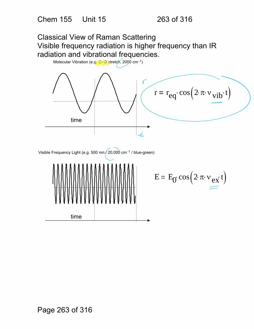
Chem 155 Unit 15 263 of 316
Page 263 of 316
Classical View of Raman Scattering Visible frequency radiation is higher frequency than IR radiation and vibrational frequencies. Molecular Vibration (e.g. C=O stretch, 2000 cm -1)
Visible Frequency Light (e.g. 500 nm / 20,000 cm -1 / blue-green)
r req cos 2 π⋅ νvib⋅ t⋅( )⋅
time
E E0 cos 2 π⋅ νex⋅ t⋅( )⋅
time
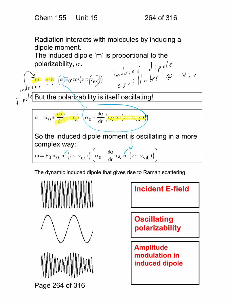
Chem 155 Unit 15 264 of 316
Page 264 of 316
Radiation interacts with molecules by inducing a dipole moment. The induced dipole ‘m’ is proportional to the polarizability, α. m α E⋅ α E0⋅ cos 2 π⋅ νex⋅ t⋅( )⋅ But the polarizability is itself oscillating! α α0
dαdr
r re−( )+ α0dαdr
rA cos 2 π⋅ νvib⋅ t⋅( )⋅( )⋅+
So the induced dipole moment is oscillating in a more complex way: m E0 α0⋅ cos 2 π⋅ νex⋅ t⋅( )⋅ α0
dαdr
rA⋅ cos 2 π⋅ νvib⋅ t⋅( )⋅+⎛⎜⎝
⎞⎟⎠
⋅
The dynamic induced dipole that gives rise to Raman scattering:
Incident E-field
Oscillating polarizability
Amplitude modulation in induced dipole
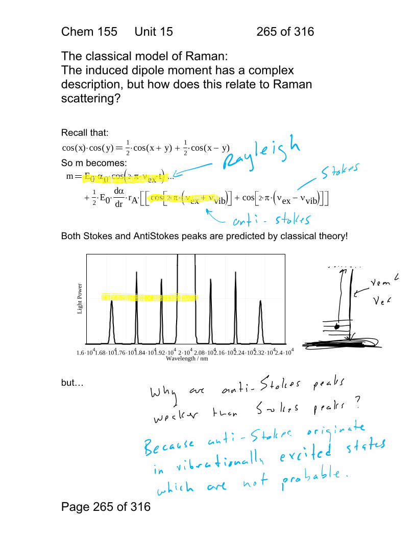
Chem 155 Unit 15 265 of 316
Page 265 of 316
The classical model of Raman: The induced dipole moment has a complex description, but how does this relate to Raman scattering? Recall that: cos x( ) cos y( )⋅
12
cos x y+( )⋅12
cos x y−( )⋅+
So m becomes: m E0 α0⋅ cos 2 π⋅ νex⋅ t⋅( )⋅
12
E0⋅dαdr
⋅ rA⋅ cos 2 π⋅ νex νvib+( )⋅⎡⎣ ⎤⎦ cos 2 π⋅ νex νvib−( )⋅⎡⎣ ⎤⎦+⎡⎣ ⎤⎦⎡⎣⋅+
...
Both Stokes and AntiStokes peaks are predicted by classical theory!
but…
1.6 .1041.68 .1041.76 .1041.84 .1041.92 .104 2 .104 2.08 .1042.16 .1042.24 .1042.32 .1042.4 .104
Wavelength / nm
Ligh
t Pow
er
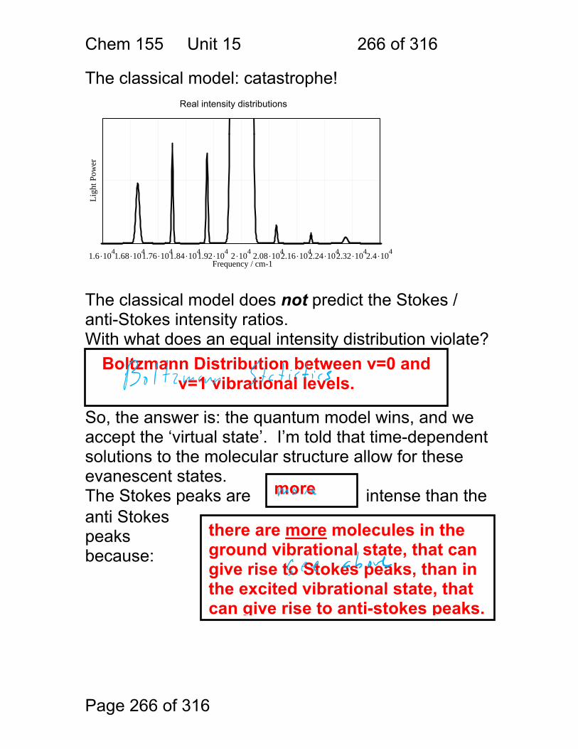
Chem 155 Unit 15 266 of 316
Page 266 of 316
The classical model: catastrophe!
The classical model does not predict the Stokes / anti-Stokes intensity ratios. With what does an equal intensity distribution violate? So, the answer is: the quantum model wins, and we accept the ‘virtual state’. I’m told that time-dependent solutions to the molecular structure allow for these evanescent states. The Stokes peaks are intense than the anti Stokes peaks because:
1.6 .1041.68 .1041.76 .1041.84 .1041.92 .104 2 .104 2.08 .1042.16 .1042.24 .1042.32 .1042.4 .104
Frequency / cm-1
Ligh
t Pow
erReal intensity distributions
Boltzmann Distribution between v=0 and v=1 vibrational levels.
there are more molecules in the ground vibrational state, that can give rise to Stokes peaks, than in the excited vibrational state, that can give rise to anti-stokes peaks.
more
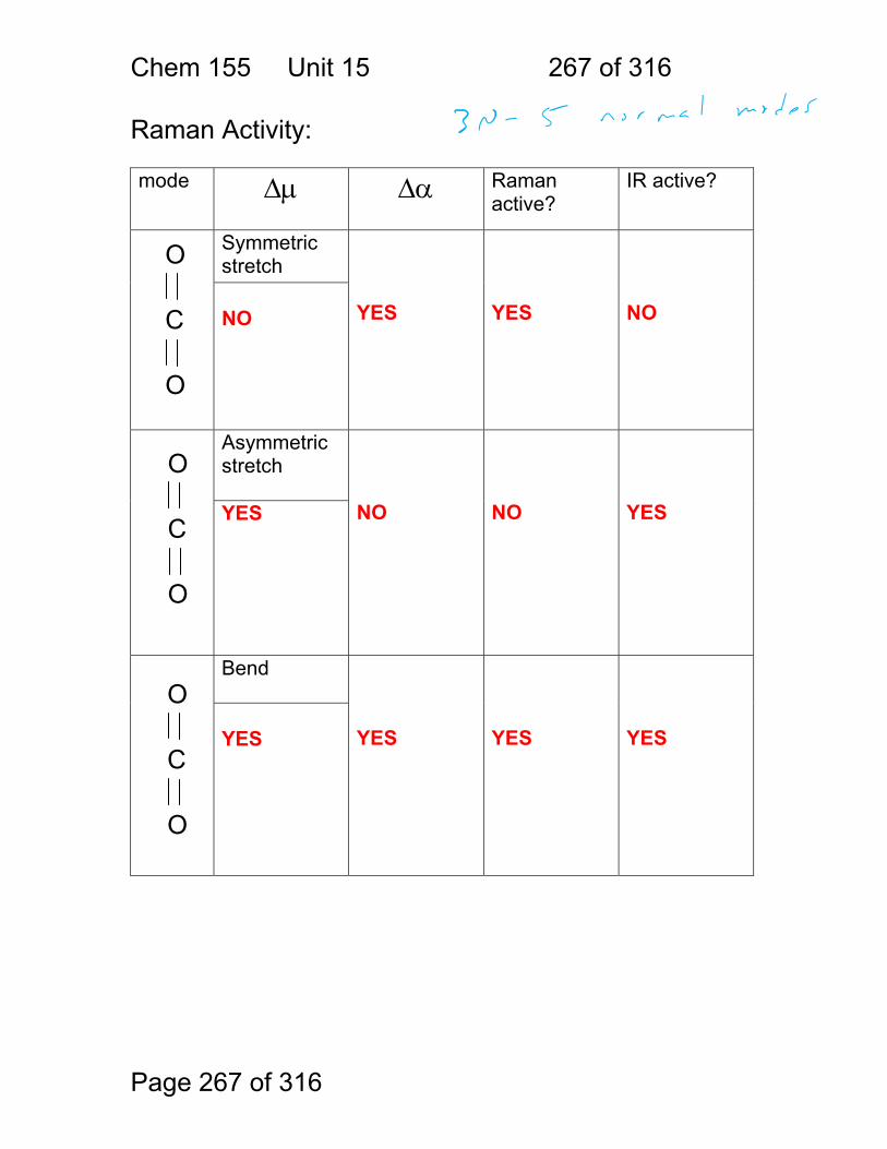
Chem 155 Unit 15 267 of 316
Page 267 of 316
Raman Activity: mode Δμ Δα Raman
active? IR active?
Symmetric stretch
YES
YES
NO
NO
Asymmetric stretch
NO
NO
YES YES
Bend
YES
YES
YES
YES
O
O
C
O
O
C
O
O
C
Chem 155 Unit 15 268 of 316
Page 268 of 316
Also note that: Purely centro-symmetric modes are only Raman active, but IR inactive. Most modes are both Raman and IR allowed. Many allowed modes may be too weak to detect in either Raman or IR or both. Intensity distributions between Raman and IR often differ substantially.
Chem 155 Unit 15 269 of 316
Page 269 of 316
Some general points regarding Raman: Pro: Raman uses visible light: Optics Solvents Biological samples Imaging with Raman has better spatial resolution because of the shorter wavelengths used. Microscopes can be used in ‘Raman microprobe’ mode. Silver and gold particles or rough surfaces can very strongly enhance Raman scattering. Different vibrational modes can be seen (e.g. centrosymmetric)
Very low frequency modes are accessible (e.g. inorganics): Depolarization ratio can distinguish between symmetric and asymmetric stretches.
ν vib12π
kμ
⋅
Chem 155 Unit 15 270 of 316
Page 270 of 316
Con: Raman signals are often very weak. High-powered lasers can damage samples, so this is not always a good solution. Fluorescent molecules can give bad spectral interference for Stokes lines.
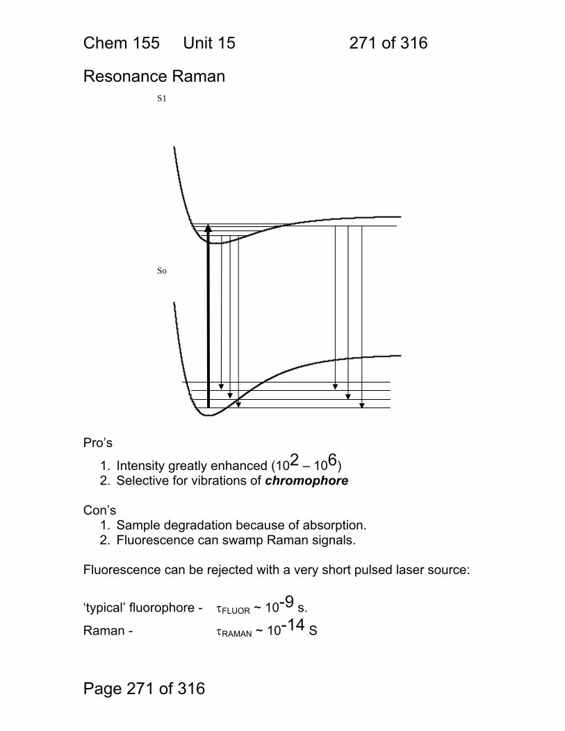
Chem 155 Unit 15 271 of 316
Page 271 of 316
Resonance Raman
Pro’s
1. Intensity greatly enhanced (102 – 106) 2. Selective for vibrations of chromophore
Con’s
1. Sample degradation because of absorption. 2. Fluorescence can swamp Raman signals.
Fluorescence can be rejected with a very short pulsed laser source:
‘typical’ fluorophore - τFLUOR ~ 10-9 s.
Raman - τRAMAN ~ 10-14 S
So
S1
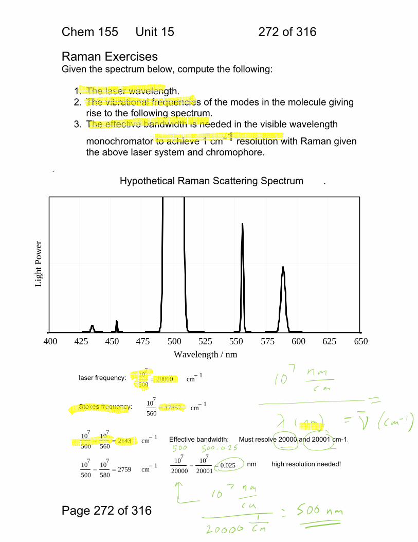
Chem 155 Unit 15 272 of 316
Page 272 of 316
Raman Exercises Given the spectrum below, compute the following:
1. The laser wavelength. 2. The vibrational frequencies of the modes in the molecule giving
rise to the following spectrum. 3. The effective bandwidth is needed in the visible wavelength
monochromator to achieve 1 cm-1 resolution with Raman given the above laser system and chromophore.
.
400 425 450 475 500 525 550 575 600 625 650Wavelength / nm
Ligh
t Pow
er
Hypothetical Raman Scattering Spectrum .
laser frequency: 107
50020000= cm 1−
Stokes frequency: 107
56017857= cm 1−
107
500107
560− 2143= cm 1− Effective bandwidth: Must resolve 20000 and 20001 cm-1.
107
20000107
20001− 0.025= nm high resolution needed!107
500107
580− 2759= cm 1−
Chem 155 Unit 15 273 of 316
Page 273 of 316
4. Using and Ar-ion laser at 514.5nm, at what wavelength would you expect to see the Stokes peak for the NO2 resonance of nitrobenzene given that it is normally observed at 1520 cm-1 in IR absorption spectroscopy?
5. Does the CO bond in CO2 have a dipole moment? YES
6. Does the CO2 molecule have a dipole moment? Why? No, because individual C=O bond dipoles exactly cancel.
7. Draw a series of CO2 molecules to illustrate the symmetric stretching mode.
8. Is the CO2 symmetric stretch IR active? Why? No, because at no time during the vibration does the dipole moment change.
9. Is the CO2 symmetric stretch Raman active? Why? Yes, because during the vibration the polarizability changes.
107
514.51520− 17916= cm 1− 107
17916558.2= nm
O C O O C OO C O
Chem 155 Unit 15 274 of 316
Page 274 of 316
10. Draw a series of CO2 molecules to illustrate the
asymmetric stretching mode.
11. Is the asymmetric stretch IR active? Why? Yes, because at during the vibration the dipole moment changes.
12. Is the asymmetric stretch Raman active? Why? No, because at during the vibration the polarizability does not change. (increase in one CO bond polarizability is offset by decrease in the other bond).
13. Why is N2 not a greenhouse gas?
Homonuclear diatomics have no dipole moment change during their only vibrational mode: symmetric stretch.
O C OO CO O C O
Chem 155 Unit 15 275 of 316
Page 275 of 316
14. Cyclohexanone has a strong absorption peak at 5.86μm
and at this wavelength a linear relationship exists between absorbance and concentration.
a. Calculate the frequency of this mode in cm-1. b. Identify the part of the molecule responsible (the group
frequency) for the absorbance at this wavelength. This is the ‘carbonyl’ or ketone symmetric stretch.
c. Suggest a solvent that would be suitable for a quantitative
analysis of cyclohexanone at this wavelength. CCl4, CHCl3 or tetrachloroethylene
d. A solution of cyclohexanone (2.0 mg/mL) in the selected
solvent has an absorbance of 0.40 in a cell with a path length of 0.025 mm. What is the detection limit for this compound under these conditions, if the noise associated with the spectrum of the solvent is 0.001 absorbance units. A=εbC calibration slope = εb
104
5.861706= cm 1−
εbAC
0.40
2.00mgmL
⋅
0.2mgmL
⎛⎜⎝
⎞⎟⎠
1−= Cm
3 sb⋅
m3 0.001⋅
0.2mgmL
⎛⎜⎝
⎞⎟⎠
1−⋅
0.015mgmL
=
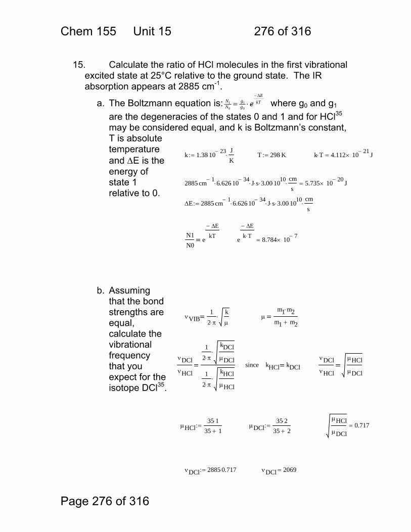
Chem 155 Unit 15 276 of 316
Page 276 of 316
15. Calculate the ratio of HCl molecules in the first vibrational
excited state at 25°C relative to the ground state. The IR absorption appears at 2885 cm-1.
a. The Boltzmann equation is: kTE
gg
NN e
Δ−
⋅=0
1
0
1 where g0 and g1 are the degeneracies of the states 0 and 1 and for HCl35 may be considered equal, and k is Boltzmann’s constant, T is absolute temperature and ΔE is the energy of state 1 relative to 0.
b. Assuming
that the bond strengths are equal, calculate the vibrational frequency that you expect for the isotope DCl35.
νDCl 2069=νDCl 2885 0.717⋅:=
μHClμDCl
0.717=μDCl35 2⋅
35 2+:=μHCl
35 1⋅35 1+
:=
νDClνHCl
μHClμDCl
kHCl kDClsinceνDClνHCl
12 π⋅
kDClμDCl
⋅
12 π⋅
kHClμHCl
⋅
μm1 m2⋅
m1 m2+νVIB
12 π⋅
kμ
⋅
e
ΔE−
k T⋅ 8.784 10 7−×=
N1N0
e
ΔE−
kT
ΔE 2885 cm 1−⋅ 6.626⋅ 10 34−
⋅ J⋅ s⋅ 3.00⋅ 1010⋅
cms
⋅:=
2885 cm 1−⋅ 6.626⋅ 10 34−
⋅ J⋅ s⋅ 3.00⋅ 1010⋅
cms
⋅ 5.735 10 20−× J=
k T⋅ 4.112 10 21−× J=T 298 K⋅:=k 1.38 10 23−
⋅JK
⋅:=
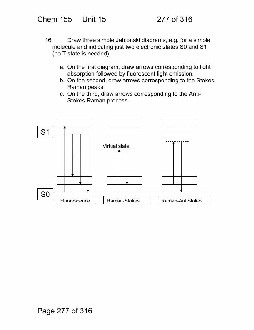
Chem 155 Unit 15 277 of 316
Page 277 of 316
16. Draw three simple Jablonski diagrams, e.g. for a simple
molecule and indicating just two electronic states S0 and S1 (no T state is needed).
a. On the first diagram, draw arrows corresponding to light
absorption followed by fluorescent light emission. b. On the second, draw arrows corresponding to the Stokes
Raman peaks. c. On the third, draw arrows corresponding to the Anti-
Stokes Raman process.
Fluorescence Raman-Stokes Raman-AntiStokesS0
S1
Virtual state
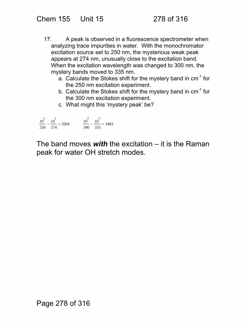
Chem 155 Unit 15 278 of 316
Page 278 of 316
17. A peak is observed in a fluorescence spectrometer when
analyzing trace impurities in water. With the monochromator excitation source set to 250 nm, the mysterious weak peak appears at 274 nm, unusually close to the excitation band. When the excitation wavelength was changed to 300 nm, the mystery bands moved to 335 nm.
a. Calculate the Stokes shift for the mystery band in cm-1 for the 250 nm excitation experiment.
b. Calculate the Stokes shift for the mystery band in cm-1 for the 300 nm excitation experiment.
c. What might this ‘mystery peak’ be?
107
250107
274− 3504=
107
300107
335− 3483=
The band moves with the excitation – it is the Raman peak for water OH stretch modes.
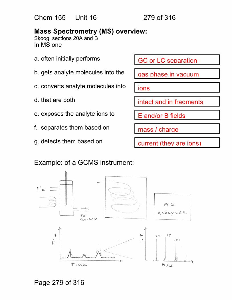
Chem 155 Unit 16 279 of 316
Page 279 of 316
Mass Spectrometry (MS) overview: Skoog: sections 20A and B In MS one
a. often initially performs
b. gets analyte molecules into the
c. converts analyte molecules into
d. that are both
e. exposes the analyte ions to
f. separates them based on
g. detects them based on
Example: of a GCMS instrument:
ions
gas phase in vacuum
intact and in fragments
E and/or B fields
mass / charge
current (they are ions)
GC or LC separation
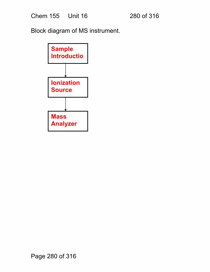
Chem 155 Unit 16 280 of 316
Page 280 of 316
Block diagram of MS instrument.
Sample Introductio
Ionization Source
Mass Analyzer
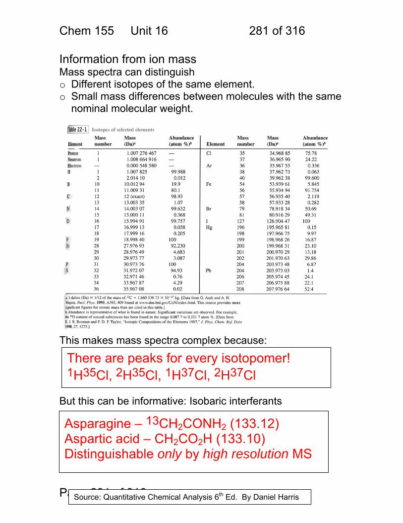
Chem 155 Unit 16 281 of 316
Page 281 of 316
Information from ion mass Mass spectra can distinguish o Different isotopes of the same element. o Small mass differences between molecules with the same
nominal molecular weight.
This makes mass spectra complex because: But this can be informative: Isobaric interferants
There are peaks for every isotopomer! 1H35Cl, 2H35Cl, 1H37Cl, 2H37Cl
Asparagine – 13CH2CONH2 (133.12) Aspartic acid – CH2CO2H (133.10) Distinguishable only by high resolution MS
Source: Quantitative Chemical Analysis 6th Ed. By Daniel Harris
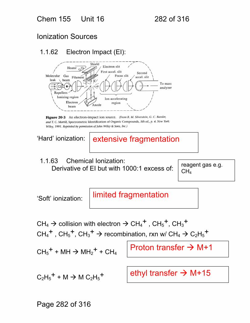
Chem 155 Unit 16 282 of 316
Page 282 of 316
Ionization Sources 1.1.62 Electron Impact (EI):
‘Hard’ ionization: 1.1.63 Chemical Ionization:
Derivative of EI but with 1000:1 excess of: ‘Soft’ ionization: CH4 collision with electron CH4+ , CH5+, CH3+ CH4+ , CH5+, CH3+ recombination, rxn w/ CH4 C2H5+ CH5+ + MH MH2+ + CH4 C2H5+ + M M C2H5+
reagent gas e.g. CH4
Proton transfer M+1
ethyl transfer M+15
extensive fragmentation
limited fragmentation
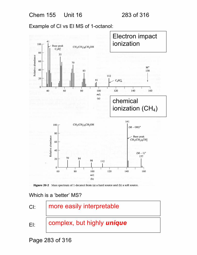
Chem 155 Unit 16 283 of 316
Page 283 of 316
Example of CI vs EI MS of 1-octanol:
Which is a ‘better’ MS? CI: EI:
Electron impact ionization
chemical ionization (CH4)
more easily interpretable
complex, but highly unique
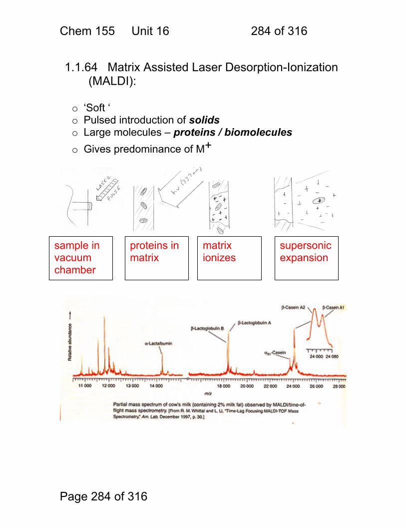
Chem 155 Unit 16 284 of 316
Page 284 of 316
1.1.64 Matrix Assisted Laser Desorption-Ionization
(MALDI): o ‘Soft ‘ o Pulsed introduction of solids o Large molecules – proteins / biomolecules o Gives predominance of M+
sample in vacuum chamber
proteins in matrix
matrix ionizes
supersonic expansion

Chem 155 Unit 16 285 of 316
Page 285 of 316
1.1.65 Electrospray Ionization (ESI): o ‘Soft ‘ o Continuous introduction of solids o Large molecules – proteins / biomolecules o Gives many different charge states: M+ , M+2 , M+3 ,
M+4 , M+5 etc.
What happens when charged droplets dry out?
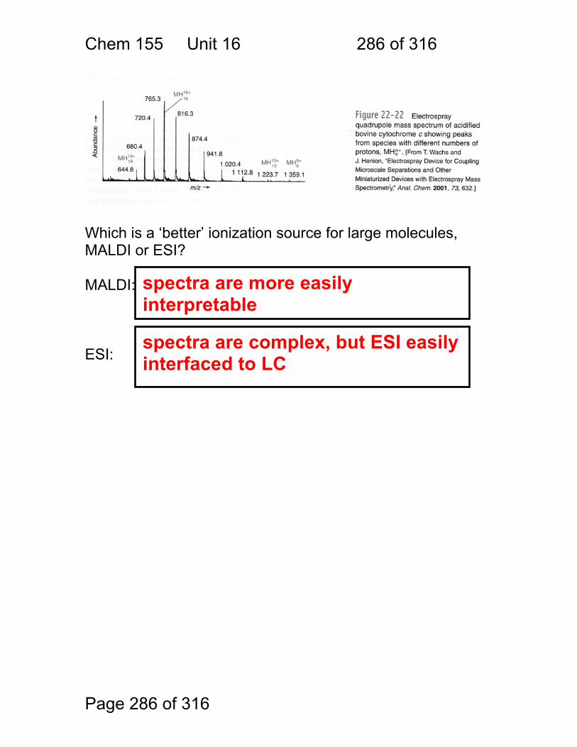
Chem 155 Unit 16 286 of 316
Page 286 of 316
Which is a ‘better’ ionization source for large molecules, MALDI or ESI? MALDI: ESI:
spectra are more easily interpretable
spectra are complex, but ESI easily interfaced to LC
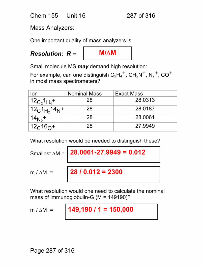
Chem 155 Unit 16 287 of 316
Page 287 of 316
Mass Analyzers: One important quality of mass analyzers is: Resolution: R ≡ Small molecule MS may demand high resolution: For example, can one distinguish C2H4+, CH2N+, N2+, CO+ in most mass spectrometers? Ion Nominal Mass Exact Mass 12C21H4+ 28 28.0313
12C1H214N+ 28 28.0187
14N2+ 28 28.0061
12C16O+ 28 27.9949 What resolution would be needed to distinguish these? Smallest ΔM = m / ΔM = What resolution would one need to calculate the nominal mass of immunoglobulin-G (M = 149190)? m / ΔM =
28.0061-27.9949 = 0.012
28 / 0.012 = 2300
M/ΔM
149,190 / 1 = 150,000
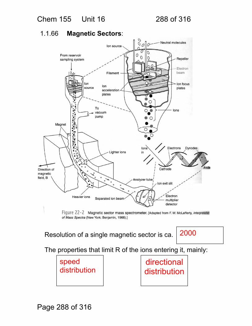
Chem 155 Unit 16 288 of 316
Page 288 of 316
1.1.66 Magnetic Sectors:
Resolution of a single magnetic sector is ca. The properties that limit R of the ions entering it, mainly:
speed distribution
directional distribution
2000

Chem 155 Unit 16 289 of 316
Page 289 of 316
1.1.67 Double-Focusing Electric Magnetic Sectors Electric Sector Focuses: Magnetic Sector Re-focuses: At double-focus point, all ions have narrow speed and direction distributions, so only ions of a given M/z exit at that point. What determines the M/z values that exit? R attainable:
Speed distribution
Directional distribution
E-field on electric sector
B-field on magnetic sector
100,000
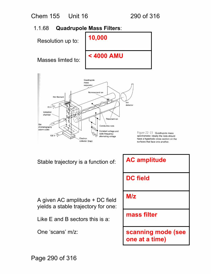
Chem 155 Unit 16 290 of 316
Page 290 of 316
1.1.68 Quadrupole Mass Filters: Resolution up to: Masses limted to: Stable trajectory is a function of: A given AC amplitude + DC field yields a stable trajectory for one: Like E and B sectors this is a: One ‘scans’ m/z:
10,000
< 4000 AMU
AC amplitude
DC field
M/z
mass filter
scanning mode (see one at a time)
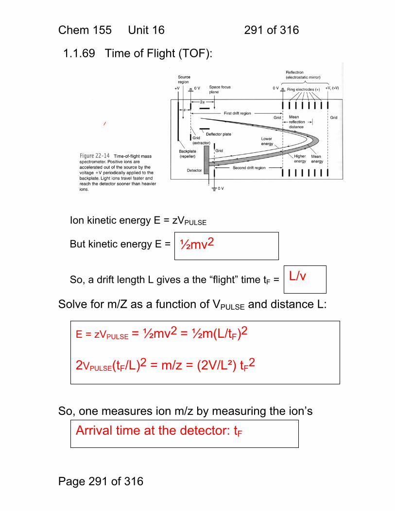
Chem 155 Unit 16 291 of 316
Page 291 of 316
1.1.69 Time of Flight (TOF): Ion kinetic energy E = zVPULSE But kinetic energy E = So, a drift length L gives a the “flight” time tF =
Solve for m/Z as a function of VPULSE and distance L: So, one measures ion m/z by measuring the ion’s
½mv2
L/v
E = zVPULSE = ½mv2 = ½m(L/tF)2 2VPULSE(tF/L)2 = m/z = (2V/L²) tF2
Arrival time at the detector: tF
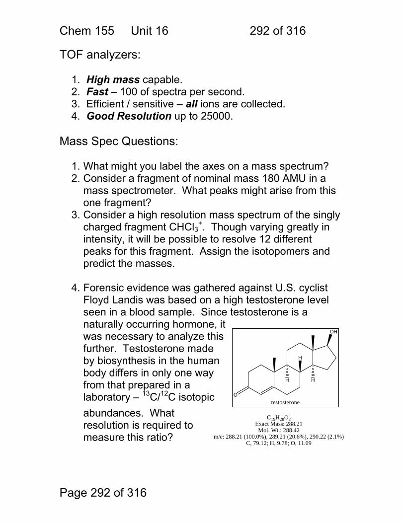
Chem 155 Unit 16 292 of 316
Page 292 of 316
TOF analyzers:
1. High mass capable. 2. Fast – 100 of spectra per second. 3. Efficient / sensitive – all ions are collected. 4. Good Resolution up to 25000.
Mass Spec Questions:
1. What might you label the axes on a mass spectrum? 2. Consider a fragment of nominal mass 180 AMU in a
mass spectrometer. What peaks might arise from this one fragment?
3. Consider a high resolution mass spectrum of the singly charged fragment CHCl3+. Though varying greatly in intensity, it will be possible to resolve 12 different peaks for this fragment. Assign the isotopomers and predict the masses.
4. Forensic evidence was gathered against U.S. cyclist
Floyd Landis was based on a high testosterone level seen in a blood sample. Since testosterone is a naturally occurring hormone, it was necessary to analyze this further. Testosterone made by biosynthesis in the human body differs in only one way from that prepared in a laboratory – 13C/12C isotopic abundances. What resolution is required to measure this ratio?
O
OH
H
H
H
testosterone
C19H28O2Exact Mass: 288.21Mol. Wt.: 288.42
m/e: 288.21 (100.0%), 289.21 (20.6%), 290.22 (2.1%)C, 79.12; H, 9.78; O, 11.09
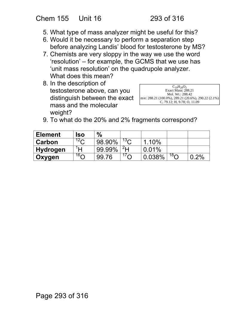
Chem 155 Unit 16 293 of 316
Page 293 of 316
5. What type of mass analyzer might be useful for this? 6. Would it be necessary to perform a separation step
before analyzing Landis’ blood for testosterone by MS? 7. Chemists are very sloppy in the way we use the word
‘resolution’ – for example, the GCMS that we use has ‘unit mass resolution’ on the quadrupole analyzer. What does this mean?
8. In the description of testosterone above, can you distinguish between the exact mass and the molecular weight?
9. To what do the 20% and 2% fragments correspond?
Element Iso % Carbon 12C 98.90% 13C 1.10% Hydrogen 1H 99.99% 2H 0.01% Oxygen 16O 99.76 17O 0.038% 18O 0.2%
C19H28O2Exact Mass: 288.21Mol. Wt.: 288.42
m/e: 288.21 (100.0%), 289.21 (20.6%), 290.22 (2.1%)C, 79.12; H, 9.78; O, 11.09