CHEM 366 FALL 2006

CHEMISTRY 361

QUANTUM CHEMISTRY

AND

CHEMICAL KINETICS

Enrique Peacock-Lopez1, ∗

1Department of Chemistry

Williams College

Williamstown, MA 01267

(Dated: June 17, 2006)

Abstract

The early XX century saw the birth of the theory of relativity. This theory was developed after

the 1887 Michelson and Morley’58 experiment which was designed to reveal the earth’s motion

relative to the ether. In an effort to explain the experimental facts, Poincare and Einstein altered

the ideas and concept of space, time and astronomical distances. Most of the development of the

the theory of relativity was carried out by the latter scientists. In contrast Quantum chemistry took

several decades and many contributors to be developed. This theory can be seen as an extension

of classical mechanics to the subatomic, atomic and molecular sizes and distances.

In this course we will study the fundamental theory of electrons, atoms and molecules known

as Quantum Chemistry. In our approach we will follow the historical development of Quantum

Chemistry. In this approach we will see how Quantum Chemistry gradually evolves from confusion

and dilemma into a formal theory.

∗Author to whom correspondence should be addressed. Electronic address: epeacock@williams.edu

1

Lecture 1

As we have seen in previous chapters, the world we experience with our senses is a world

described by Thermodynamics, Classical Mechanics and Classical Electromagnetism. It is

a macroscopic world based in macroscopic laws. But scientist have long recognized exper-

imentally the existence of small particles which are the components of matter. Therefore

it is natural to look first for microscopic laws that explain the particle’s behavior, and sec-

ond we have to look for a theoretical approach that will link the microscopic laws with the

macroscopic laws.

Towards the end of the XIX century, many physicist felt that all the principles of physics

had been discovered and little remainded to be understood except for few minor problems.

At that time our world was understood using Classical Mechanics, Thermodynamics and

Classical Electromagnetism. For example in Classical Mechanics or Newtonian Mechanics

we needed to find the dynamical variables of the system under study. Once done this, we

needed to construct the equation of motion which predicted the system’s evolution in time.

The predicted behavior was finally compared with the experimental observations.

At the time the Universe was divided into matter and radiation. Matter was ruled

by Newtonian mechanics and thermodynamics, and radiation obeyed Maxwell’s laws of

Electromagnetism. A controversy whether light was wave-like or corpuscular-like existed

since Newton’s days, who proposed the corpuscular theory of light. The wave-like theory

was developed by Huggens based in the constructive and destructive interference of light; a

property which is characteristic of waves.

The interaction between matter and radiation was not well understood. For example,

Earnshaw’s theorem states that a system of charged particles can not remain at rest in

stable equilibrium under the influence of purely electrostatic forces. Moreover, according

to Electromagnetism an accelerated charged particles radiate energy in the form. of elec-

tromagnetic waves. Thus how is that molecules are stable? From this minor problems the

theory of Quantum chemistry was developed.

2

Lecture 2

During the 17th century Galileo Galilei and Issac Newton postulated a corpuscular theory

of light. After 200 years of work, in the 19th century we have a logical theory with determin-

istic equation that explain planetary motion as well as classical mechanics, thermodynamics,

optics, electricity and magnetism.

In the mid 1800s, Thomas Young reported a pattern consisting of dark and bright fringes,

which were produces after passing light through two narrow closely spaced holes or slits. This

interference pattern is a natural wave behavior. By 1860, James Clark Maxwell developed a

classical electromagnetic theory, which combines electricity and magnetism in a single theory.

Also, Maxwell’s theory predicts that the properties of light can be explained if we consider

light as electromagnetic radiation. The experimental confirmation of maxwell equation was

reported by Michael Faraday, and 1886, although assuming a luminiferous (ether) medium,

Hertz confirmed experimentally that light is electromagnetic radiation giving the wave theory

of light a solid foundation.

In 1887, Albert Michelson and edward Morley’1860, confirmed experimentally the elec-

tromagnetic waves traveled in vacuum by finding no difference in the speed of light relative

to the motion of Earth. In other word, there is no need of the luminiferous or any other

medium. Without a medium, light is subject to a relativistic description that was developed

by Poincare and Einstein.

From the classical Maxwell equations, we can prove Earnshaw’s Theorem, which states

that a system of charged particles can not remain at rest in stable equilibrium under the

influence of purely electrostatic forces. In other words, accelerated charged particles radiate

energy in the form of electromagnetic waves. So how atoms and molecules are stable? or

how atoms and molecules absorb and emit radiation only at certain frequencies?

Electromagnetic waves

Electromagnetic waves are made up of an oscillating electric (E), and a perpendicular

magnetic (B) and are produced by accelerated charges, where the electric field E displaces

charged particles along the direction of the field, and the magnetic field B rotates charged

particles around the direction of the field.

3

The electric field in units of volt m−1 and pointing in the Z-direction is described

Ez(y, t) = Eo Sin(k y − w t) (1)

where the angular frequency is defined as

w = 2πν‘, (2)

the wave vector as

k =2 π

λ, (3)

and Eo is the amplitude of the electric field. The magnetic field pointing in the X-direction

is described

Bx(y, t) =Eo

cSin(k y − w t)‘, (4)

where

λ ν ‘ = c =w

k(5)

A single wavelength, λ, implies monochromatic light, where the range of wave lengths varies

from:

Cosmic Rays

λ = 3 10−24 m ν = 1032 s−1 4x1017 eV

l

Long radio waves

λ = 3 106 m ν = 102 s−1 4x10−13 eV

When Electro Magnetic radiations (light) interacts with matter, it gets scattered. In the

case of scattering from many centers, we say that light gets diffracted. In contrast, when

light gets scattered by few centers, we say that light shows interference.

4

Lecture 3

Blackbody radiation

Experimentally we observe that when a metallic object is heated it would change its

color. As the temperature is increased, first the object changes its color into a dull red and,

progressively, becomes more and more red. Eventually it changes from red to blue. As it

is well established experimentally, the radiated energy is associated with a color which is

associated to a frequency or wavelength. To understand this phenomenon, we will consider

a so-called black-body

An ideal object that absorbs and emits all frequencies is defined as a black-body. It is a

theoretical model invented by theorist to study the emision and absorbtion of radiation. Its

experimental counterparts consist of an insulated box which can be heated. On one of its

faces a small pinhole allows radiation to enter or leave. This radiation is equivalent to that

of a perfect black-body.

One of the “minor” problems mention earlier relates to the density of radiated energy

per unit volume per unit frequency interval dν at temperature T, ρ(ν, T ). The search for

an expression for ρ(ν, T ) backs to 1860 when Gustav Kirchhoff recognized the need of a

theoretical approach to blackbody radiation. Also the relation between ρ(ν, T ) with certain

empirical equations was not well understood. In 1899 Wien noticed that the product of

temperature ,T, and maximum wavelength, λmax was always a constant,

T λmax = constant. (6)

Equation 6 is called the displacement law. Also the total energy radiated per unit area per

unit time, R, from a blackbody followed Stefan-Boltzman law,

R = σ T 4 , (7)

where σ is a constant. These two empirical law needed to be explained from first principles.

In 1896 Wilhem Wien derived the following expression for ρ:

ρ(ν, T ) = C ν3 exp{−a ν

T

}, (8)

where C and a are constants. Wien’s result was experimentally confirmed for high frequencies

by Freiderich Paschen in 1897. But in 1900, Otto Lummer and Ernest Pringsheim found

5

that Wien’s expression failed in the low frequency regime. The first attempts to explain

0.0 500.0 1000.0 1500.0 2000.0Wavelength / nm

0.0

0.5

1.0

1.5

Ene

rgy

dens

ity

per

wav

elen

gth

(10

J /m

)

6000 K

5000 K

4000 K

3000 K

Classical 3000 K

FIG. 1: Plank’s radiation density for a blackbody.

the previous empirical laws from first principles used the classical knowledge at the time.

For example in 1900 Rayleigh assumed that the radiation trapped in the box interacted

with the walls. On the walls small oscillators which in turm vibrate emiting radiation.

Finally the equilibrium between the “oscillators” and the radiation trapped in the box is

responsable of the properties of black-body radiation. Under these assuptions, the density

of radiated energy per unit volume per unit frequency at temperature T is given by the

following equation:

ρ(ν, T ) dν = Nν dν ε(ν, T ) , (9)

where Nν dν represents the number of oscillators between ν and ν + dν, and ε(ν, T ) is the

average energy radiated by the “electronic oscillator” at frequency ν and temperature T.

The number density was widely accepted to be

Nν =8π ν2

c3(10)

6

where c is the speed of light.

In the calculation of ε(ν, T ) Reyleigh assumed that the“oscillators” could achieve any

possible energy and the equipatition theorem. In other words Rayleigh assumed a continuous

energy spectrum for the oscillators and

ε(ν, T ) = kBT , (11)

where kB is Boltzman constant. With these assumptions, Rayleigh obtained the following

expression for the amount of radiative energy between ν and ν + dν:

ρ(ν, T ) dν =8π ν2

c3kBT dν . (12)

If we express Eq. 12 as radiated energy per unit volume per unit wavelength we get

ρ′(λ, T ) dλ =8π

λ4kBT dλ , (13)

where we have used the relation c = λν. This latter result agreed with the low frequency

observation but did not fit the experimental observationsm at high frequencies.

From the low and high frequency expressions,

ε(ν, T ) ≈

kBT for low ν

ν exp{− a ν

T

}for high ν

, (14)

Planck derived an expression consistent with both limiting behaviors,

ε(ν, T ) =h ν

exp{

hνkBT

}− 1

. (15)

This expression required only one constant, h, which Plank determined by fitting the ex-

pression to the experiemntal data. Equation 15 is called the Plank distribution law. Plank

obtained an excellent agreement with experiments using

h = 6.626× 10−34 J s . (16)

Although Eq. 15 fitted the experiemntal data extraordinary well, Plank wanted to un-

derstand why Eq. 15 worked so well. First Plank calculated the entropy of the system from

15. Second, he calculated the entropy using Boltzman mechanistic approach. When these to

independent expression for the entropy were compared, Plank concluded the the oscillators

7

spectrum had to be discrete. In other words the “oscillators” could only achive the following

energy values:

εn = n h ν , (17)

where n is a positive integer and h is Plank’s constant. Thus both of Plank’s entropy

expression were consisten if energy was quantized.

From Max Planck’s underlying assuption that the energies of the “electronic oscillators”

could have only a discrete set of values we can derived the semiempirical Plank’s distribution

using statistical methods. In this approach we assumed that only jumps of ∆n = ±1 can

occur, so the change of energy is given by:

∆ε = h ν . (18)

This means that energy is absorbed or emitted only in packets.

In order to obtain an expression for the density of radiative energy between ν and ν+ dν

we have to calculate the average energy, ε(ν), at frequency ν. First we consider the Boltzman

probability for the energy level of each oscillator at frequency ν, i.e.,

Pn(ν) ≈ exp

{n hν

kBT

}. (19)

Using Eq. 19 we get for the average oscillator’s energy

ε(ν) =

∑∞n=1 nhν exp

{n hνkBT

}∑∞

n=1 exp{

n hνkBT

}=

∑∞n=1 nhν Xn∑∞

n=1 Xn

=hν X

(1−X)2

11−X

=hν X

1−X

=hν

exp{

hνkBT

}− 1

. (20)

Finally using Eqs. 9 and 10 the Plank’s expression for the radiative energy density is equal

to

ρ(ν, T ) dν =8π ν2

c3hν

exp{

h νkBT

}− 1

dν . (21)

8

Also as a function of wavelength we get

ρ′(λ, T ) dλ =8π hc

λ5

1

exp{

h ckBT λ

}− 1

dλ . (22)

From Eq. 22 we can obtain the Wien displacement law and the Stefan-Boltzman law.

9

Lecture 4

Photoelectric effect

Late in the 19th century a series of experiments revealed that electrons are emitted from

a metal surface when light of sufficient high frequency falls upon it. This is known as the

photoelectric effect. Classical theory predicted that the energy of the ejected electron is

proportional to the intensity of the light; electrons are ejected for any frequency radiated.

Both prediction are not support by the experients.

The experiemnts show the existance of a threshold frequency, ν◦. Einstein in 1905 as-

sumed that radiation consists of little packets of energy ε = hν. If this is true the kinetic

energy of the ejected electron is given by the following equation:

KE =1

2mv2 = hν − φ (23)

where φ is the work function which is usually expressed in electron volts, eV. Note that the

threshhold frequency, ν◦, implies no kinetic energy. Thus

hν◦ = φ, (24)

and the photoelectric effect is observed only if hν ≥ φ. Equation 23 represents a straight

line with slope h. Actually in an experiment one measures the stopping potential, VS, such

that

KE = − e VS =1

2mv2 . (25)

10

Lecture 5

Wave equation

In this section we discuss the wave equation for a string attached at both ends. In

this case we consider a string along the x-axis with displacement in the y-direction. The

string’s displacement will be denoted as u(x,t). Finally if we consider a string of length `

the displacement satisfies the following equation:

∂2u

∂x2=

1

v2

∂2u

∂t2, (26)

where v is the magnitud of the velocity of the wave along the string. Next we consider the

boundary conditions (BC). These are the vaues of u at the ends of the string. Since the

ends are attached to say a wall, these points do not displace from its position,

u(0, t) = 0 = u(`, t) . (27)

Notice that these values are valid for any time t. Thus we have a partial differential equa-

tion and its boundary conditions for a string. This equation is commonly refered as a

1-dimensional wave equation.

Of the different methods of solution of partial differerntial equations, we will consider the

method of separation of variables. In this method we consider the the solution to Eq. 26

can be written as a product of a function of time and function of space, i.e.,

u(x, t) = X(x) T (t) . (28)

If we substitute Eq. 28 in Eq. 26 we get

T (t)d2 X(x)

d x2=

1

v2X(x)

d2 T (t)

d t2. (29)

Notice that the partial derivatives have transformed to regular derivatives since they are

applied to single variable function. Now if we divide both sides of Eq. 29 by Eq. 28 we get

1

X(x)

d2 X(x)

d x2=

1

v2 T (t)

d2 T (t)

d t2. (30)

In Eq. 30 the left hand side is a function only of position x; the right hand side is a function

only of time. Since position and time are independent variables the only posibility that

satisfies Eq. 30 is1

X(x)

d2 X(x)

d x2= α , (31)

11

1

T (t)

d2 T (t)

d t2= α , (32)

where α is a constant.

For the spatial function X(x) we have now the following equation:

d2 X(x)

d x2= α X(x) (33)

From Eq. 27 the boundary conditions for X(x) are

X(0) = X(`) = 0 . (34)

Thus we are looking for a function that satifies Eq. 33 and vanishes at x = 0 and x = `. After

some thinking we find that the function sin(x) and cos(x) satisfy the differential equation

but only sin(x) satifies the boundary condition at x = 0. In other words, if

X(x) = A sin(κ x) , (35)

Eq. 33 reduces to

d2 A sin(κ x)

d x2= − A κ2 sin(κ x)

= − κ2 X(x)

= α X(x) . (36)

Therefore

α = − κ2 . (37)

Next we consider the boundary condition

sin(κ`) = 0 . (38)

Equation 38 is satified if the argument of the sine function is an integer multiple of π,

κ ` = n π . (39)

Solving for κ we find that the spatial solution of Eq. 26 to be

X(x) = An sin(π`n x

). (40)

And the displacement u(x, t) can be written as

un(x, t) = T (t) An sin(π`n x

). (41)

12

Equation 40 represents standing waves, and the wavelength of these standing waves, λn

satisfy the following relation:π

`n λn = 2π . (42)

Thus λn is equal to

λn =2 `

n, (43)

where n is an integer greater than one. Using this result we can express κ in terms of λn,

κ =2 π

λ, (44)

and plugg it in Eq. 31 to get the following equation:

d2 X(x)

d x2= −

(2π

λn

)2

X(x) . (45)

Equation 45 represents the wave equation satified by the spatial part of the amplitud, u(x, t).

Particle’s wave equation

Since particles behave as waves we need a wave equation for a particle. A simple approach

is to use de Broglie’s assumption in Eq. 45. Namely we substitute the value of the wavelength

associated to a particle with momentum p,

λ =h

p, (46)

in the right hand side of Eq. 45. This substitution yields the following equation:

d2 ψ(x)

d x2= −

(p~

)2

ψ(x) , (47)

where ψ is the wave associated to a particle with momentum p and ~ ≡ h/2π. Now if we

recall the expression for the mechanical energy of a particle with momentum p in a potential

V (x),

E =p2

2 m+ V (x) , (48)

and solve for p2 we get

p2 = 2 m [E − V (x)] . (49)

Equation 49 can be used in Eq. 47 and get

d2 ψ(x)

d x2= − 2m

~2[E − V (x)] ψ(x) . (50)

13

Finally we can rewrite Eq. 50 as

− ~2

2 m

d2 ψ(x)

d x2+ V (x) ψ(x) = E ψ(x) . (51)

Equation 51 is the time-independent Schrodinger equation. Although this derivation is not

formal, nor Schrodinger “official” derivation, it obtains the quantization of the energy, in

the case of the hydrogen atom, as a consequence of the properties of the wave function ψ(x).

Schrodinger success attacted the attention of scientist and change the world.

Schrodinger equation

− h2

2m

∂2

∂x2Φ(x, t) + V (x) Φ(x, t) = i h

∂

∂tΦ(x, t) . (52)

Separation of variables

Φ(x, t) = φ(t) ψ(x) (53)

− 1

ψ(x)

h2

2m

d2

d x2ψ(x) + V (x) =

i h

φ

d

dtφ(t) = constant = E (54)

d φ(t)

dt= − i E

hφ(t) (55)

φ(t) = exp

{− i E

ht

}(56)

− ~2

2m

d2

d x2ψ(x) + V (x) ψ(x) = E ψ(x) (57)

14

Lecture 6

Axiomatic quantum mechanics

Classical mechanics deals with position (~r), momentum (~p), angular momentum (L ≡

mvr) and energy. These quantities are called dynamical variables. A measurable dynamical

variable is called an observable.

Time evolution of the system’s observables is governed by Newton’s equations, which

yield the system’s trajectory. In Quantum mechanics the Uncertanty Principle forbides the

concept of trajectory. Thus we need another approach to study the microscopic world of the

atom. I this section we consider an axiomatic approach. Namely we will state a number of

axioms or postulates which define the foundation of quantum mechanics. The postulates are

justified only by their ability to predict and correlate experimental facts and their general

applicability.

1. Postulate 1

The state of a quantum-mechanical system is completely specified by a function Ψ(~r, t).

This function is called the wave function or the state function.

The probability of finding the particle in a volume element dV arround ~r at time t is

given by:

P(~r, t) = |Ψ(~r, t)|2 dV = Ψ∗(~r, t) Ψ(~r, t) dV , (58)

where the star, Ψ∗ represents the complex conjugate of the wave function Ψ. As a conse-

quence of the probabilistic interpretation, the probability of finding the particle some place

in the space is equal to unity or ∫Space

|Ψ(~r, t)|2 dV = 1 . (59)

This condition puts some requirements on the kind of state function that we can consider.

For example Ψ and d Ψ/d~r have to be continous, finite and single-valued (for each position

~r only one value of Ψ(~r, t).

15

2. Postulate 2

For any observable in classical mechanics, we cam find a corresponding quantum mechan-

ical operator. For example momentum in the x direction:

px = m vx ←→ p = − i ~d

d x, (60)

angular momentum in the x direction:

Lx = y pz − z py ←→ Lx = − i ~{y∂

∂z− z

∂

∂y

}, (61)

energy:

E =p2

2m+ V (x) ←→ H = − ~2

2m

d2

dx2+ V (x) . (62)

3. Postulate 3

When an observable, corresponding to A, is measured, the only values observed are given

by:

A Ψn = an Ψn , (63)

where an is a set of eigenvalues called the spectrum of A. What if the system is in some

arbitrary state, Ψ, which is not the eigenfunction of A?

4. Postulate 4

The expected value of A when Ψ is not an eigenfunction of A is given by:

〈 A 〉 ≡∫

Space

Ψ∗ AΨ dV . (64)

5. Postulate 5

The time dependence of Ψ(~r, t) is given by the time-dependent Schrodinger equation,

H Ψ(~r, t) = i ~∂

∂ tΨ(~r, t) . (65)

If the the hamiltonian, H, does not include time explicitely, the wave function can be written

as a product of two functions,

Ψ(~r, t) = ψ(~r) f(t) . (66)

16

As we have mention earlier this separation of variables leads to the time independent

Schrodinger equation

H ψ(~r) = E ψ(~r) . (67)

The solution of Eq. 67 implies a set of energies {En} i.e.,

H ψn(~r) = En ψn(~r) , (68)

where ψ′ns are called the stationary states, and each state is characterized by an energy En.

In this sense we say that the energy is quantized.

Also we can solve the time dependent differential equation and find

f(t) = exp

{− i

En

~t

}, (69)

which means that the time dependent wave function is given by the following expression:

Ψ(~r, t) = ψ(~r, t) exp

{− i

En

~t

}. (70)

Since the energy is quantized, we represent an atom or molecule by a set of stationary

energy states. The spectroscopic properties of the system will be understood in terms of

transitions from one stationary state to another. The energy associated with the transition

is equal to:

∆En→m = Em − En = hν , (71)

where ν is the frequency of the photon either emitted or absorbed.

In general the system is not going to be in a stationary state ψn. In this case we can ask

How many atoms are in each stationary state ψn? Since the system is not in a stationary state

we can construct a wave function for the system as a linear combination of the stationary

states ψn. In other words the system’s wave function is given by:

Φ(~r, t) =∞∑

n=1

Cn ψn(~r) exp

{− i

En

~t

}. (72)

Therefore the probability of measuring a particular En value in a series of observations is

proportional to the square of its coefficient Cn, i.e., C∗C = |C|2.

17

Lecturel

I. INTRODUCTION

For the last twenty-five years sustained oscillations of the concentration of a chemical

substance have been the subject of intensive study. In spite of theoretical predictions of

damped oscillations and sustained oscillations by Lotka and Hirniakand [7, 8] in 1910

and Lotka [9] in 1920, and the experimental observation of cyclic changes in the iodate

catalyzed decomposition of hydrogen peroxide by Bray in 1921[10], both experimentalists

and theorists virtually ignored the field of chemical oscillations. The First Symposium on

Biological and Biochemical Oscillators was organized in 1968, forty seven years after Bray’s

paper appeared in the Journal of the American Chemical Society.

In the early 1950’s Belusov [11] observed cyclic color changes in the bromination of citric

acid catalyzed by cerium. However, the world scientific community did not gain access to

the experimental details of these cyclic color changes, since Belusov’s first findings were

rejected for publication in 1951, and another six years of detailed experimentation were

again rejected in 1957 [12]. Out of his work Belusov published an abstract in an obscure

symposium in 1959 [11] and kept the original manuscript; he never tried again to publish

his results. For years the Belusov protocol for chemical oscillations was known only to

researchers and students at the Moscow State University, until one of those students,

Zhabotinsky, initiated a careful and detailed investigation of the Belusov reaction during

the first half of the 1960’s. In the final analysis, Zhabotinsky substituted citric acid for

malonic acid and published his findings in 1964 [13]. By 1967 the first paper written in

English reached the West, causing inmense interest among many researchers.

An interesting aspect of the Belusov-Zhabotinsky (B-Z) reaction centers around the orig-

inal motivation that led Belusov to the celebrated reaction. Originally, his interest in bio-

chemistry, and in particular in the Krebs cycle [14], motivated Belusov to seek a simple

experimental model in which a carbohydrate was oxidized in the presence of a catalyst. In

other words, the B-Z reaction was intended as a model of an enzyme catalyzed reaction.

This connection between enzyme kinetics and the B-Z reaction is often forgotten and rarely

18

mentioned. Most likely, this omission can be traced to the differences between an enzyme

and its model counterpart Ce, the complicated mechanism underlining the chemical oscilla-

tions in the B-Z reaction and the mathematical analyses needed to understand some of the

reduced models of the B-Z reaction. From the biochemical point of view, these differences

are difficult to reconcile with a biological model. Therefore, the search for a model of chem-

ical oscillation in enzyme kinetics that is both biochemically relevant and mathematically

simple enough to present to an undergraduate audience is worthwhile from the pedagogical

point of view.

In the present discussion we consider glycolysis, centering around the allosteric properties

of phosphofructokinase (PFK). For nearly thirty years oscillations in the concentration of

nucleotides in the glycolitic pathway have been documented in the case of yeast cells and cell-

free extract [15]. For example, reduced nicotinadenine dinucleotide (NADH) oscillations in

yeast extract have been observed and determined to be flux dependent; a minimum external

flux is required to sustain oscillations in the concentration of NADH. Moreover, Hess and

Boiteux [16] observed that phosphofructokinase plays an essential role in these oscillations. If

PFK’s substrate, fructose-6-phosphate ( F-6-P), is added to cell-free extracts, the nucleotide

concentrations oscillate. On the other hand, after the injection of PFK’s product, fructose-

1,6-bisphosphate (F-1,6-bP), no oscillations are observed. Based on these observations and

on the allosteric properties of PFK, two models were suggested in the late 1960’s. One, by

Higgins [17], is based on the activation of PFK by its product. The second model [18] is

based on the activation and inhibition properties of PFK by adenosine triphosphate (ATP),

adenosine diphosphate (ADP) and adenosine nonophosphate (AMP). The latter links PFK

with pyruvate kinase, while the former does not.

In the next section we discuss the steps along the glycolytic pathway which are relevant

to the Higgins model. Next we reduce the model to two variables and discuss its similarities

with Lotka’s models and the origin of the autocatalytic step. Finally, we scale the model, do

a linear stability analysis and discuss the bifurcation diagram of the reduced, two-variable

Higgins model.

19

II. HIGGINS MODEL

The interest in the origin of periodic biological processes like the circadian clock has

motivated researchers to look for the chemical basis of oscillations in biochemical systems

[19]-[21]. One of these systems is glycolysis, in which six-membered sugars are converted

anaerobically into tricarbonic acids. This process allows the phosphorylation of ADP. In

the case of glycolysis the addition of glucose to an extract containing the main metabolites

triggers cyclic, or periodic, behavior in the concentrations of metabolites. This periodic

change in the concentrations of the glycolytic metabolites is termed glycolytic relaxation

oscillations. In particular, relaxation oscillations in the concentration of NADH are readily

observed using spectrophotometric methods on yeast extracts. For the past twenty-five years,

researchers have studied mostly relaxation oscillations which are due to a single injection

of glucose. In this case, the system relaxes to equilibrium. Conversely, if constant or

periodic injection is applied, a system is pushed away from equilibrium and can achieve

nonequilibrium steady states.

Researchers have found that phosphofructokinase (PFK), which catalyzes the conversion

of F-6-P to F-1,6-bP, is the regulatory enzyme for glycolytic oscillations [22]-[23]. This

regulation is the result of the activation and inhibition properties of PFK. For example, in

liver, PFK is activated by F-2,6-bP [24] which is an isomer of F-1,6-bP. And in muscle, PFK

is inhibited by ATP. Based on these facts, most kinetic models of glycolytic oscillations have

centered around either PFK’s inhibition [18] or its activation [17]. One of the models based

on the activation of PFK by fructose biphosphate is the Higgins model. This model considers

only two enzymatic reactions with a constant external source of glucose. Condensing two

steps of the glycolytic path into one, the Higgins model assumes a first order conversion

of glucose to F-6-P. Following this first step, the Higgins model considers the enzymatic

conversion of F-6-P to F-1,6-bP by PFK and F-1,6-bP to glyceraldehyde-3-phosphate (G-

3P) by aldolase (ALD). In this model, the regulation consists only of the activation of

an inactive Phosphofructokinase (PFK) by F-1,6-bP. Under this assumption, the Higgins

model sustains oscillations in the concentration of F-6-P, F-1,6-P and the enzymes. Using

further simplifications, such as the steady-state approximation for PFK, the model reduces

to three time-dependent species with autocatalytic conversion of F-6-P to F-1,6-bP. Finally,

if one considers a steady-state approximaztion for ALD, one obtains a two-species model

20

which is able to sustain oscillations.

The following equations depict the steps along the glycolytic pathway that are relevant

to the Higgins model:

Glucose (G)k◦−→ (F − 6− P ) (73a)

F − 6− P + (PFK)K1

F − 6− P − PFK (73b)

F − 6− P − PFK k1−→ (F − 1, 6− bP ) + PFK (73c)

F − 1, 6− bP + (ALD)K2

F − 1, 6− bP − ALD (73d)

F − 1, 6− bP − ALD k2−→ 2 (G− 3− P ) + ALD (73e)

(PFK) + F − 1, 6− bP Ka−→ PFK . (73f)

For the sake of a simple notation, the following mechanism, which is equivalent to Eq.

(73b)-(73f), will be used:

G◦k◦−→ X (74a)

X + E1

K1

XE1 (74b)

Y + E2

K2

Y E2 (74c)

XE1k1−→ Y + E1 (74d)

Y E2k2−→ Z + E2 (74e)

Y + E1

Ka

E1 . (74f)

where G stands for glucose, X for F-6-P, E1 for PFK, Y for F-1,6-bP and E2 for ALD.

Using these equations, the mass action laws for the six species model are as follows:

d[X]

dt= koG◦ − k+

E1[E1][X] + k−E1

[E1X] (75a)

d[Y ]

dt= k1[E1X]− k+

E2[E2][Y ] + k−E2

[E2Y ]− k+a [E1][Y ] + k−a [E1] (75b)

d[E1]

dt= k−E1

[E1X]− k+E1

[E1][X] + k1[E1X]− k−a [E1] + k+a [E1][Y ] (75c)

d[E1X]

dt= −k−E1

[E1X] + k+E1

[E1][X]− k1[E1X] (75d)

d[E2]

dt= k−E2

[E2Y ]− k+E2

[E2][Y ] + k2[E2Y ] = −d[E2Y ]

dt. (75e)

Using the steady-state approximation for all of the enzymes, we obtain a minimal two

21

variable model [25]

d[X]

dt= koG◦ − kac[X][Y ] (76a)

d[Y ]

dt= kac[X][Y ]−

V2m[Y ]

K2M

1 + [Y ]K2M

, (76b)

where kac is given by the following equation:

kac =Ka

V1m

K1M

1 +Ka[Y ] + Ka

K1M[X][Y ]

(77a)

KiM =ki + k−Ei

k+Ei

(77b)

Vim = ki E◦i (77c)

Ka =k+

a

k−a. (77d)

(77e)

In Eq.(77d) E◦i represents the stochiometric concentration of the ith enzyme. Also in the

Higgins model, kac is simplified even further to

kac =V1mKa

K1M

=k1k

+E1E◦

iKa

k1 + k−E1

. (78)

Equations (76b)-(78) constitute the Minimal Higgins (MH) model .

A. Comparison with the Lotka Model

The Minimal Higgins Model as expressed by Eqs. (76b) and (76b) shows some similar-

ities with the Lotka’s models. For example, in the original Lotka model of 1910, species

reproduction is proportional to the amount of food, which is kept constant; namely

GkR−→ R (79)

This elementary step, in conjunction with the following steps:

R +WkW−→ 2W (80a)

WkD−→ D (80b)

define what is known as the Lotka Model and the differential equations describing the time

behavior of the population are given in Table I.

22

Table I

Model Differential equations

Lotka 1910d[R]dt

= kRG◦ − kW [R][W ]

d[W ]dt

= kw[R][W ]− kD[W ]

Lotka 1920d[R]dt

= kRG◦[R]− kW [R][W ]

d[W ]dt

= kw[R][W ]− kD[W ]

Minimal Higginsd[X]dt

= k◦G◦ − kac[X][Y ]

d[Y ]dt

= kac[X][Y ]− V2m[Y ]K2M + [Y ]

Schankenbergd[X]dt

= k◦G◦ − kS[X][Y ]2

d[Y ]dt

= ks[X][Y ]2 − kD[Y ]

Notice that the first differential equations in the MH model and the Lotka’s 10 model are

the same. In the 1920 paper, Lotka introduced a species dependent external flux, namely

G+RkR2−→ 2R (81)

which is a autocatalytic step and substitutes Eq.(79). In this case, the differential equations

describing the time behavior of the populations are given in Table I. In both Lotka’s models

cases, the concentration of grass, G◦, is kept constant. Notice that the 1920 model is a

variation of the 1910 model which yields oscillation in the population. Consequently, we

23

can think of the MH model as a variation of the 1910 model where we have included an

enzymatic step instead of a first order step.

These two Lotka models are the simplest schemata in which oscillations in the popula-

tions can be observed. A meaningful interpretation of this model is in population dynamics.

For example if we define G as grass, R as rabbit and W as wolf, the explanation of the

oscillatory behavior seems quite logical. As the rabbits consume the grass and reproduce,

their numbers grow, while the amout of grass decreases. As the rabbit population grows, the

wolves have plenty of rabbits available for consumption, and they, too, reproduce. However,

as the wolf population increases, the rabbit population decreases. As the rabbit population

decreases, the wolves start to die, since there are not enough rabbits. As a consequence,

grass becomes more plentiful, and the rabbits start the cycle again. Unfortunately, the first

Lotka model yields only damped oscillation and the second model gives sustained oscilla-

tions for any initial condition, which is a severe restriction if we want to model realistic

chemical and biochemical system. In contrast, the Minimal Higgins model shows stable

steady states, damped and sustained oscillations. The richness of this model stems from

the second differential equation which includes an enzymatic Michaelis-Menten step. More-

over, the autocatalytic step in the MH model can be traced to the activation of PFK by

its product. The fourth model in Table I is due to Schnakemberg [28]. In this model, the

bimolecular autocatalytic step in the Lotka 1910 model is replaced by a trimolecular step.

This change appears as a cubic term in the differential equations. With this change, the

model shows sustained oscillations. But the connection between the cubic autocatalytic

term and a biochemical justification has not been achieved.

III. STABILITY ANALYSIS

In this section we present a linear stability analysis [26] of the Minimal Higgins model.

For this purpose, we scale the differential equation such that the dimensionless differential

equations depend only on two parameters rather than on five. Namely, we get from Eqs.

(76b)-(76b)

dX

dτ= A − XY (82a)

dY

dτ= XY − qY

1 + Y, (82b)

24

where we have defined the following dimensionless quantities:

τ = kacK2M t (83a)

X =[X]

K2M

(83b)

Y =[Y ]

K2M

(83c)

A =k◦G◦

K22Mkac

(83d)

q =V2m

K22Mkac

(83e)

The first step in the stability analysis is to find the steady state solution. In general this is

done by setting the left hand side of the differential equations equal to zero and solving for

the concentrations. From Eqs.(82b)-(82b), we obtain for the scaled MH model the following

steady state solutions:

xss = q − A (84a)

yss =A

q − A. (84b)

Clearly form Eqs.(84b)-(84b), we can see that the physically meaningful solutions have to

satisfy the following condition: q > A. Only values of A less than q give meaningful physical

results, i.e., xss and yss have to be positive.

Once these stationary states are obtained, stability analysis studies what happens to all

components of the system when the system is perturbed slightly from its steady state. For

this purpose we first calculate the relaxation matrix, R, which is the Jacobian associated to

a set of ordinary differential equations (ODEs) [26]. For the scaled MH model, we obtained

the following matrix:

R =

−yss −xss

yss xss − q(1+yss)2

. (85)

Next, we have to find the eigenvalues, λ±of R, which are the solutions of the following

characteristic polynomial:

λ2 +

[(1 + yss)(yss − xss) + xss

1 + yss

]λ+

[xssyss

1 + yss

]= 0 . (86)

In this case the solutions of the quadratic Eq.( 86) are

λ± = −1

2

[(1 + yss)(yss − xss) + xss

1 + yss

]± 1

2

√[(1 + yss)(yss − xss) + xss

1 + yss

]2

− 4

[xssyss

1 + yss

](87)

25

Equation (87) can be reduced to the following expression:

λ± =PR(A, q)±

√PI(A, q)

2q(q − A), (88)

where we have defined the following functions:

PR(A, q) = A[A2 − 2Aq + q2

](89)

PI(A, q) = A[A5 − 4qA4 + 2q(3q + 1)A3 − 4q2(q + 2)A2 + q2(q2 + 10q + 1)A− 4q2

](90)

Equations (89,90) have been obtained both by analytical methods and with the help of the

software package MATHEMATICA [27].

From Eqs.(87)-(90) , we can analyze four possible eigenvalues: a) PR < 0 and PI > 0.

In this case, the eigenvalue is pure real and negative. Thus the steady state solution is a

stable fixed point [26]. b)PR < 0 and PI < 0. In this case, the eigenvalue has a negative

real part and a nonzero imaginary part. For this eigenvalue, we find damped oscillations.

c)PR > 0 and PI > 0. In this case, the eigenvalue is pure real and positive. The steady

state is unstable. d)PR > 0 and PI < 0. In this case, the eigenvalue has a positive real part

and a nonzero imaginary part. The steady state is unstable and moves away to unstable

oscillations.

Also, we can construct a plot of A vs. q. Figure 1, depicts such a diagram, and the

different lines represent curves where A - q, PR and PI are equal to zero. These curves

delimit different regions in parameter space. In region A, we observe stable fixed points, in

region B, we observe damped oscillations, and region C, we observe sustained oscillations.

For a fixed value of q, the value of A at which PR(A, q) is equal to zero, Ac, defines the

bifurcation point. Values of A greater than Ac are in regions A orB, and for values less than

Ac are in region C. Thus for Ac < A < q the system reaches a fixed point e.g. Figure 2 and

3. For A < Ac, the systems reaches a limit cycle e. g. Figure 4. The diagram of A versus

oscillation amplitude is called a bifurcation diagram [26] depicted by Figure 5.

The only problem with the Minimal Higgins model is a fixed point at y = 0 and an

infinite large value of x. For a fixed q this case occurrs for small values of A, where also

numerical integration becomes problematic. For this reason the biburcation diagram only

considers values of A greater than 2. This particular problem is also present in the Lotka’s

models as well as in the Schnakenberg model [28].

26

2 4 6 8 10

q

0

2

4

6

8

10

A

FIG. 2: Parameter space diafram for the Minimal Higgins model. Region A is limited by he line

q = A and PR(A, q) = 0; Region B is limuted by PR(A, q) = 0 and PI(A, q) = 0; Region C is define

by PI(A, q) > 0.

IV. SUMMARY

The minimal Higgins model is a simple two species model that shows sustained oscillations

in enzyme kinetics. The steps in the mechanism have a biochemical justification and the

step responsible of the oscillation is a Michaelis-Menten step. Also, the stability analysis is

simple and accessible both analytically or with the help of MATHEMATICA. For example

the bifurcation points are obtained by fixing either A or q and solving a simple quadratic

equation, e.g. Equation(89).

The only problem associated with the MH model and inherent to all of the models in

Table I is a fixed point at y = 0 and an infinite large value of x. Numerically and for fixed q,

the problem appears for small values of A. In some cases, MATHEMATICA is not able to

handle the numerical integrations and other algorithms are required to study the differential

27

0 10 20 30 40 50 60 70

t

0

1

2

3

4

5

6

7

X

a)

2.5 5 7.5 10 12.5 15 17.5 20

X

0

2.5

5

7.5

10

12.5

15

17.5

20

Y

A = 8.5

FIG. 3: Example from region A. In this case q = 10 and A = 8.50. a) x vs t; b) x vs. y.

equations for small values of A [? ? ]. Modification intended to remove this kind of fixed

points have been done for the Schnakenberg model. For example, the addition of a first

order convertion of x into y i.e.

k`

X −→ Y(91)

yield the two-variable autocatalator model. Also, the well known Brusselator can be obatined

from the Schnakenberg model by replacing the first order formation of X by

kb1 (92)

kb2

B + Y −→ X.(93)

Although these models do not have fixed points at infinity, a biochemical justification for

those steps does not exist. In the case of the MH model similar modifications can be

done to remove the fixed point at infinity. In these case, the modification have a plausible

28

0 10 20 30 40 50 60 70

t

0

1

2

3

4

5

X

a)

2.5 5 7.5 10 12.5 15 17.5 20

X

0

2.5

5

7.5

10

12.5

15

17.5

20

Y

A = 6.87

b)

FIG. 4: Example from region B. In this case q = 10 and A = 6.87 a) x vs t; b) x vs. y.

explanation. For example, synthesis of glycogen could prevent infinitely large values of X.

And from high levels of glycogen, an eventual formation of F-1,2-bP can be assume. These

two steps have the equivalent effect as Eq. (91).

In summary, the Minimal Higgins model provides us with a simple system of non-linear

differential equations that can be biochemical justified. Also, the model’s stability analysis

is easy to handle both analitically or with the help of MATHEMATICA. This yields simple

study of the bifurcation diagrams.

29

0 10 20 30 40 50 60 70

t

0

1

2

3

4

5

6

7

X

a)

2.5 5 7.5 10 12.5 15 17.5 20

X

0

2.5

5

7.5

10

12.5

15

17.5

20

Y

A = 6.50

b)

FIG. 5: Example from region C. In this case q = 10 and A = 6.50. a) x vs t; b) x vs. y.

V. GENERAL MODEL

In previous work [? ]−[? ] we have considered Rebek’s self-replicating system and mod-

eled ideal self-replication using a self-complementary template mechanism. For this mech-

anism we used a reasonable chemical model that is consistent with the laboratory work on

self-replication. In particular, we have focused on a simple self-replicating mechanism; how-

ever, in general, chemical self-replication can be represented schematically by the following

mechanistic steps:

where T represents the self-replicating molecule and A and B are the component frag-

ments. In the uncatalyzed step, components A and B “collide” with a relative low probability

to form the template, T. The structure of the product T is such that once it is formed, it

preferentially binds A and B in a conformation that facilitates covalent bonding between

the A and B molecules to form another T molecule. The newly created template and the

original template molecules then split apart and independently catalyze further reactions.

30

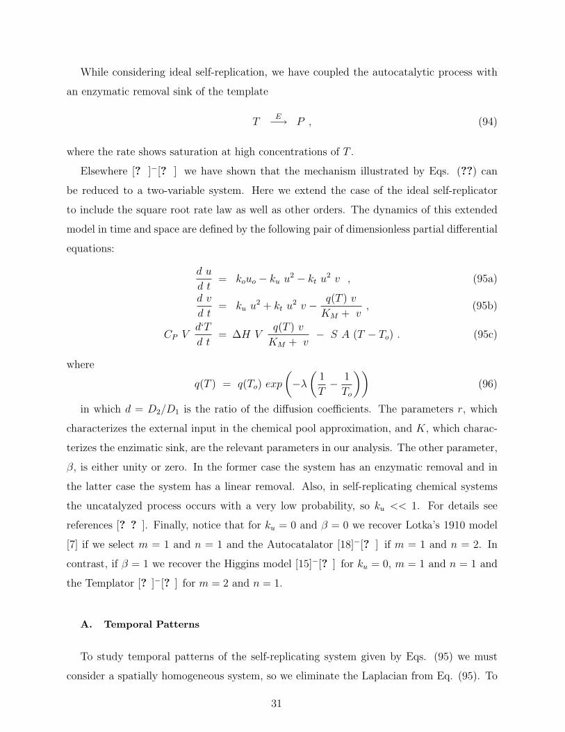
While considering ideal self-replication, we have coupled the autocatalytic process with

an enzymatic removal sink of the template

TE−→ P , (94)

where the rate shows saturation at high concentrations of T .

Elsewhere [? ]−[? ] we have shown that the mechanism illustrated by Eqs. (??) can

be reduced to a two-variable system. Here we extend the case of the ideal self-replicator

to include the square root rate law as well as other orders. The dynamics of this extended

model in time and space are defined by the following pair of dimensionless partial differential

equations:

d u

d t= kouo − ku u

2 − kt u2 v , (95a)

d v

d t= ku u

2 + kt u2 v − q(T ) v

KM + v, (95b)

CP Vd‘T

d t= ∆H V

q(T ) v

KM + v− S A (T − To) . (95c)

where

q(T ) = q(To) exp

(−λ

(1

T− 1

To

))(96)

in which d = D2/D1 is the ratio of the diffusion coefficients. The parameters r, which

characterizes the external input in the chemical pool approximation, and K, which charac-

terizes the enzimatic sink, are the relevant parameters in our analysis. The other parameter,

β, is either unity or zero. In the former case the system has an enzymatic removal and in

the latter case the system has a linear removal. Also, in self-replicating chemical systems

the uncatalyzed process occurs with a very low probability, so ku << 1. For details see

references [? ? ]. Finally, notice that for ku = 0 and β = 0 we recover Lotka’s 1910 model

[7] if we select m = 1 and n = 1 and the Autocatalator [18]−[? ] if m = 1 and n = 2. In

contrast, if β = 1 we recover the Higgins model [15]−[? ] for ku = 0, m = 1 and n = 1 and

the Templator [? ]−[? ] for m = 2 and n = 1.

A. Temporal Patterns

To study temporal patterns of the self-replicating system given by Eqs. (95) we must

consider a spatially homogeneous system, so we eliminate the Laplacian from Eq. (95). To

31

find the conditions for chemical oscillations, we first find the steady state (u, v) of Eq. (95),

v =r K

1− β r, (97a)

u =

(r

ku + vn

) 1m

, (97b)

where we notice that, since v > 0, βr < 1. This condition reduces the size of the parameter

space considerably.

Next we reduce the Jacobian to the following form:

J =

− m ru

− n rv

+ kun un

v

m ru

(n−1)r+β r2

v− ku

n un

v

, (98)

and calculate the determinant of the Jacobian at the steady state.

detJu,v = mr2

u v(1− β r) =

mr2(1− βr)2 [Knrn + ku(1− βr)n ]1/m

Kr1+m

m (1− βr) nm

≥ 0 . (99a)

Since βr < 1, the determinant of the Jacobian at the steady state is always positive for all

non-zero m and all n, and thus the stability of the steady states is determined by the sign

of the trace of the Jacobian.

The trace of the Jacobian evaluated at the steady state is given by a somewhat more

complicated expression,

trdJu,v =F

K [Knrn + ku(1− βr)n] (1− βr) nm

, (100a)

where we have defined

trdJu,v ≡ d J11 + J22 (100b)

and

F ≡[(n− 1− βr)Knrn − ku(1− βr)n+1

](1− βr)

m+nm

− (md)Krm−1

m [Knrn + ku(1− βr)n]m+1

m . (100c)

Notice that in Eq. (100b) we have included the dimensionless diffusion coefficient d. In this

section we will consider the case d = 1, but for spatial patterns we must analyze Eq. (100b)

with d < 1 .

32

Depending on the relative sizes the terms in Eq. (100c), the trace may be positive or

negative. In particular we are interested in finding when, for d = 1, the trace greater or

equal to zero, so we consider the following equation:[(n− 1 + βr)Knrn − ku(1− βr)n+1

](1− βr)

m+nm −

(m)Krm−1

m [Knrn + ku(1− βr)n]m+1

m ≥ 0 .(101)

The inequality in Eq. (101) implies that the steady state is unstable and therefore small

homogeneous perturbations grow over time. The equality, which we can rewrite as

K =(1− βr)

[(n− 1 + βr)− ku

(1−βr)n+1

Knrn

] mm+n

mm

m+n rm+n−1

m+n

[1 + ku

(1−βr)n

Knrn

] m+1m+n

, (102)

defines an exact transcendental equation that, when solved for K, yields a Poicare-Adronov-

Hopf (PAH) bifurcation.

Notice that for ku = 0 we obtain an exact analytical solution for the PAH bifurcation for

any values of m and n provided (n−1+βr) ≥ 0. Another relevant limiting case is the linear

removal in Eqs. (95) that we recover when β = 0 and K = 1, which yields the following

bifurcation relation:

Kbif =[n− 1]

mm+n

mm

m+n rm+n−1

m+n

. (103)

From Eq. (101) we need that (n− 1) ≥ 0. This last constraint requires a value of n greater

than unity. Therefore the smallest nonlinearity coupled with a linear sink that is able to

sustain oscillations is the so-called Autocatalator, in which m = 1 and n = 2.

In contrast, when β = 1 we get an enzymatic sink in Eq. (95), and for ku = 0 we get the

following analytical bifurcation relation:

Kbif =(1− r) [(n− 1 + r)]

mm+n

mm

m+n rm+n−1

m+n

, (104)

in which (n− 1 + r) ≥ 0. Notice that n no longer has to be greater than unity in a system

with m and n greater than zero. As long as (n − 1 + r) ≥ 0, the system shows a PAH

bifurcation. For example, for β = 1, m = 2 and n = 1 we recover the Templator model with

a cubic nonlinearity and for β = 1, m = 1, and n = 1 we recover the Higgins model which

contains a quadratic nonlinearity.

Moreover, for β = 1, m = 1/2 and n = 1/2, the system with nonlinearity m + n = 1

shows oscillations if

K ≤ (1− r)√

2 r − 1 , (105)

33

where 1/2 ≤ r ≤ 1. In summary, the inclusion of an enzymatic sink instead of a linear

sink in Eq. (95) allows the systems with nonlinearities less than cubic to sustain oscillations.

Since we already derived a general bifurcation condition for this system in terms of the

parameters and m and n, to obtain a bifurcation diagram for the generalized model, we

simply set m = 1, n = 1/2, ku = 0.01 and β = 1 and then plot the bifurcation condition

given by Eq. 102 to visualize the relationship between K and r. In Figure (??A) we depict

the curve tr J = 0, in which, for a given value of K, we can find two PAH bifurcation points

as we vary r. In addition, if the parameter values fall within the loop, the trace of the

Jacobian at the steady state is positive and thus the system is capable of stable oscillatory

solutions.

We repeat our analysis for m = 2 and in Figure (??B) we plot the PAH bifurcation curve.

Notice that here the area of the region in which tr J > 0 is smaller than when m = 1. Thus

when m = 2 oscillations are restricted to a smaller set of parameter values

B. Spatial Patterns

Next we consider heterogeneous perturbations which result when d < 1 and find the

conditions for Turing patterns, which are a kind of spatial pattern. [? ]−[? ] In general, for

a system to sustain Turing patterns the following four conditions must be satisfied:

detJ > 0 , (106a)

J11 + J22 < 0 , (106b)

d J11 + J22 > 0 , (106c)

(d J11 + J22)2 > 4 d detJ , (106d)

where J is the Jacobian and J11 and J22 are the diagonal elements of the Jacobian.

As discussed earlier, the determinant is always positive for physical parameter values, so

we only need to consider the final three conditions. We have already calculated expressions

for second and third inequalities in the previous section. The fourth relation yields the

34

following equation:

(md)Krm−1

m [Knrn + ku(1− βr)n]m+1

m +

2√Kmd r

m−12m [Knrn + ku(1− βr)n]

2m+12m (1− βr)

2m+n2m

−(n− 1 + βr)Knrn(1− βr)m+n

m +

ku(1− βr)2+n+n/m < 0 .

(107)

For the minimal case ku = 0 the last three Turing conditions reduce to the following

analytical expressions, respectively:

K >(1− βr) (n− 1 + βr)

mm+n

(m)m

m+n rm+n−1

m+n

(108a)

K <(1− βr) (n− 1 + βr)

mm+n

(m d)m

m+n rm+n−1

m+n

(108b)

K <(1− βr)

(√n−√

1− βr) 2m

m+n

(m d)m

m+n rm+n−1

m+n

(108c)

Moreover, the intersection of the PAH bifurcation and the Turing conditions defines a

codimension-two point where both the PAH and the Turing conditions are satisfied. This

point is easily calculated from Eqs. (108).

rc =1

β

[1−

(1− d1 + d

)2

n

], (109)

where the critical value of r depends only on d and n and is independent of m.

To find the bifurcation diagrams that illustrate the parameter values required for Turing

patterns, we first numerically solve Eqs. (106) and (107) for ku 6= 0, n = 1/2 and either

m = 1 or m = 2.

In Figure (??) we depict Eqs. (106) with curves C1 and C2. Curve C1, as in the previous

section, determines the PAH bifurcation. Curve C2 is similar to C1 but was calculated with

d = 0.20 instead of d = 1. The region between these curves is stable to homogeneous

perturbations. The fourth condition, Eq. (107), which is depicted by curve C3, delimits

the region that is unstable to inhomogeneous perturbations; therefore, points in parameter

space between curves C3 and C1 satisfy necessary conditions for Turing patterns.

35

Acknowledgments

The authors would like to thank the National Science Foundation for their financial

support through grant CHE-0136142 and CHE-0548622.

[1] L. E. Orgel, Nature 358, 203 (1992).

[2] L. E. Orgel, Acc. Chem. Res. 28, 109 (1995).

[3] T. R. Cech, PNAS 83, 4360 (1986).

[4] T. R. Cech, Nature 339, 507 (1989).

[5] G. von Kiedrowski, Amgew Chem. 25, 932 (1986),

[6] B. Bag and G. von Kiedrowski, Pure Appl. Chem. 68, 2145 (1996).

[7] Lotka, A. J. J. Am. Chem. Soc. 1910, 42, 1595-99.

[8] Hirniak, Z. Z. Physik. Chem. 1910, 675-680.

[9] Lotka, A. J. J. Phys. Chem. 1920, 14, 271-74.

[10] Bray, W. C. J. Amer. Chem. Soc. 1921, 43, 1262-1267.

[11] Belusov, B. P., Sb. Ref. Radiats. Med. za 1958.; Medgiz: Moscow 1959, 1, 145.

[12] Winfree, A. T. J. Chem Edu. 1984 , 61, 661-663 (1984)

[13] Zhabotinsky, A. M. Biofizika 1964,9 , 306. (in Russian).

[14] van Holde, M. Biochemistry; Benjamin: Redwood,1990.

[15] Gosh, A.; Chance, B. Biochem. Biophys. Res. Commun. 1964, 16, 174-81.

[16] Boiteux, A.; Hess, B.; Sel’kov E. E. Current Topics in Cellular Regulation 19xx, 17, 171-203.

[17] Higgins, J. Proc. Nat. Acad. Sci. U.S. 1964, 52, 989.

[18] Sel’kov, E. E., Europ.J. Biochem. 1968, 4, 79.

[19] Banks, H. T. Modeling and Control in the Biomedical Sciences; Springer: Berlin, 1975.

[20] Palmer, J. D., An Introduction to Biological Rhythms; Academic: New York, 1976.

[21] Berriddge, M. J.; Rapp, P. E.; and Treherne, J. E., Eds. Cellular Oscillators; Cambridge:

Cambridge, 1979.

[22] Tornhein, K. J. Theo. Biol. 1979, 79, 491-541 (1979).

[23] Tornhein, K. J. Biol. Chem. 1988, 263, 2619-2624.

[24] Pilkins, S. J.; GrannerD. K. Annu. Rev. Physiol. 1992, 54, 885-909.

36

[25] Ibanez, J.L.; Fairem and Velarde, M. G. Phys. Lett. 1976, 58A, 364.

[26] Edelstein-Keshet, L. Mathematical Models in Biology; Random: New York, 1988.

[27] Wolfran, S., MATHEMATICA Ver. 2.1, Wolfran Research (1991).

[28] Schnakenberg, J. J. Theo. Biol. 1979, 81, 389-400.

37