Child Farm Labour: Theory and Evidence

by

Sonia Bhalotra Department of Applied Economics, Cambridge University

and

Christ Heady

Department of Economics, University of Bristol

Contents: Abstract 1. Introduction 2. The Literature and Contributions of this Paper 3. Prevalence and Intensity of Child Labour 4. A Two-period Model of Child Labour 5. An Empirical Model and Estimation Issues 6. Conclusions and Policy Implications References Tables

The Suntory Centre Suntory and Toyota International Centres for Economics and Related Disciplines London School of Economics and Political Science Discussion Paper Houghton Street No. DEDPS 24 London WC2A 2AE July 2000 Tel.: 020-7955 6674

Abstract

This paper presents a dynamic model of child labour supply in a farming household. The model clarifies the roles of land, income and household size, allowing labour and credit market imperfections. If labour markets are imperfect, child labour is increasing in farm size and decreasing in household size. The effect of income is shown to depend upon whether the effective choice is between work and school or whether leisure is involved. Credit market constraints tend to dilute the positive impact of farm size and reinforce the negative effect of income. The model is estimated for rural Ghana and Pakistan. A striking finding of the paper is that the effect of farm size at given levels of household income is significantly positive for girls in both countries, but not for boys. This is consistent with the finding, in other contexts, that females exhibit larger substitution effects in labour supply. Increases in household income have a negative impact on work for boys in Pakistan and for girls in Ghana but there is no income effect for the other two groups of children. We find interesting effects of household size and composition, female headship, and mothers' post-secondary education. Keywords: Child labour, poverty, female education, agricultural households, Ghana, Pakistan. JEL Nos.: J22, O15. © The authors. All rights reserved. Short sections of text, not to exceed two paragraphs, may be quoted without explicit permission provided that full credit, including notice, is given to the source. Correspondence address: Dr Sonia Bhalotra, Department of Applied Economics, University of Cambridge, Sidgwick Avenue, Cambridge, CB3 9DE, UK: Email: sonia.bhalotra@cam.ac.uk

Summary

Objectives, Approach & Definitions

• We investigate child labour on family farms in rural Ghana and

Pakistan.

• We propose a two-period model of child labour in a farming

household that faces labour market and credit market

imperfections and we clarify the expected impact of farm size and

household income on child labour.

• Children are defined as 7-14 year-olds in Ghana and 10-14 year-

olds in Pakistan.

• The sample is restricted to households that own or operate

agricultural land.

• The dependent variable is hours of child labour and we use the

tobit estimator.

• The potential endogeneity of household income and farm size is

taken into account. For household income the OLS coefficient is

shown to carry a significant positive bias.

Theoretical Results

• Labour market imperfections create a positive effect of farm size

on child labour.

• For a given farm size, household size should have a negative

impact on child farm labour. This contrasts with the positive

effect suggested in existing work.

• Credit market constraints tend to reinforce the negative effect of

income and dilute the positive impact of farm size, controlling for

income.

Descriptive Statistics

• The incidence of child farm labour is greater in Ghana than in

Pakistan. Data on hours of work in the reference week show farm

work to be a half-time job in both countries.

• It is much more common for farm working children to combine

work with school in Ghana than in Pakistan, and in Pakistan it is

especially uncommon amongst girls.

• A substantial proportion of children in Pakistan work for wages

outside the home in addition to working on the household farm

or enterprise but child work in Ghana is exclusively for the

household.

• In both countries, a large fraction of children was neither in work

nor in school when surveyed.

• The gender differential in school attendance in rural Pakistan is

much larger than in rural Ghana. Girls in Pakistan are more

heavily engaged in farm and wage work than boys but they are

also more likely to be classed as neither in work nor in school.

Results of Data Analysis

• For a given level of household consumption, farm size has a

positive effect on the labour of girls in both countries but does not

affect boys’ work.

• The mode of operation of land (rent, sharecropping, etc) has

effects on child labour for given acreage.

• Increases in household income decrease the work of boys in

Pakistan and girls in Ghana but there is no income effect on the

work of other children.

• Child labour does not increase with household size for any of the

four groups of children. For boys in Pakistan and girls in Ghana

household size has a negative impact.

• The age-gender composition of the household has a greater

influence on child work in Pakistan than in Ghana. While

children of the household head are less likely than other children

to be in work in Ghana, the converse is true in Pakistan.

• Female-headship significantly increases the work of all children

other than boys in Ghana. The marginal effects are larger in

Pakistan, whereas the incidence of female headship is

enormously greater in Ghana.

• Mothers’ secondary education has a negative impact for boys and

girls in Pakistan and for boys in Ghana. In contrast, a negative

effect of father’s education is observed only for Pakistani girls.

• Controlling for household resources, there are some substantial

effects of community variables measuring access to school,

rainfall/irrigation and economic infrastructure.

•

1

1. Introduction

In Ghana and Pakistan, as in most developing countries, the

vast majority of working children are engaged in agricultural work

and this is predominantly on farms owned or operated by their

families (see ILO, 1996). Since land is the most important store of

wealth in agrarian societies and a substantial fraction of households

do not own land, this casts doubt on the commonly held presumption

that child labour emerges from the poorest households (e.g., US

Department of Labor (2000), Basu and Van (1998)). The theoretical

literature on child labour has emphasised credit market imperfections

(see Ranjan (1999), Lahiri and Jaffrey (1999)) to the relative neglect of

labour market imperfections. Indeed, a well-functioning labour

market is central to the seminal paper on the economics of child

labour by Basu and Van (1998). This paper emphasises that labour

market failure may explain the prevalence of child work on

household farms and enterprises, and our theoretical model

integrates this with credit market failure.

The intuition for why asset ownership may increase child

labour is straightforward. The marginal product of the family worker

(the child) is greater the greater the stock of productive assets owned

by the household. Therefore, if households with relatively large plots

of land find it difficult to hire in workers to work on the farm

(imperfect labour market), then they have an incentive to employ

their children, as long as the wealth effect of land ownership is not so

large as to dominate.

2

To the extent that households smooth their consumption over

the lifecycle, we would expect their consumption in any period to

reflect their assessment of their lifetime wealth, including the value of

their land. Therefore, conditioning on consumption (which may be

expected to produce a negative effect on child labour if child leisure

and education are normal goods), we expect farm size to mainly

capture the (positive) substitution effect on child labour (see Section

4). It is therefore interesting to examine, as is done in this paper, the

separate effects of farm size and consumption in a dynamic model

estimated on data that isolate the children of farming households.

Existing empirical studies tend to include one or the other of farm

size and consumption but seldom both, and most aggregate over all

types of child work across rural and urban regions of a country. This

makes their results difficult to interpret.

Section 4 specifies a two-period model of child labour that

shows it to be a function of both assets and income and that clarifies

the interpretation of their coefficients under imperfect labour and

credit markets. It explicitly allows for the accumulation of both work

experience and educational capital. The returns to work experience

on the household farm may be particularly high for children that

expect to inherit their parent’s land.

A difference between Ghana and Pakistan that is of particular

relevance in this paper is that the land-labour ratio is greater on

average in Ghana than in Pakistan. Other things being equal,

households in Ghana may thus be expected to employ more children

on the household farm- and this, we find, is indeed the case (Table 1).

A related fact is that the wage labour market is better developed in

3

rural Pakistan than in rural Ghana (e.g. 36% of adult men work for

wages in rural Pakistan and only 22% in rural Ghana). If this means

that it is easier in Pakistan to hire in workers on large farms instead of

using child labour, then it is again consistent with the observed fact

that Ghana has a greater fraction of children working on household

farms. However, this does not imply that children are better off in

Pakistan. While no children in the Ghana sample are in wage

employment, 6% of boys and 12% of girls aged 10-14 in Pakistan are,

and their school attendance rates are particularly low (see Table 1).

Within rural Pakistan, our data show that households that send

children in to wage work are poorer on average than households that

employ children on the family farm. Therefore the prevalence of child

wage work in Pakistan in contrast to Ghana is consistent with the

greater incidence of poverty in Pakistan as compared with Ghana

(Ray (2000) estimates that 27% of households in Pakistan fall below

the median income per adult-equivalent as compared with 14% in

Ghana). These descriptive facts motivate the analysis and underline

the importance of conditioning simultaneously on income and assets.

The underlying question of interest is whether child work on

the farm is a choice determined by, for example, relatively high

returns to experience, or whether it is the result of household poverty,

poor school access, or the difficulties of hiring in farm labour. We

explore large and rich data sets for two countries in a comparative

light with a view to furthering our understanding of this question.

Unlike most studies on this subject, we instrument income and land.

The estimated equations provide estimates of the total impact of land

size, land tenure-type, household consumption, household size,

4

parents’ education and other relevant variables on child labour.

These permit consideration of the effects on child labour of, for

example, land redistribution, income transfers and fertility change.

The paper is organised as follows. Section 2 oulines some of the

contributions of this paper in the context of the existing literature.

Section 3 presents a descriptive analysis of the extent and nature of

child labour in the rural areas of Ghana and Pakistan. The question of

whether child labour is a “bad thing” or whether some farm work

may just be good exercise and practical training1 depends upon the

hours spent in such work and the extent to which it conflicts with

school. This is discussed in Section 3, and compared across the two

countries. Section 4 presents a two-period model of child labour in a

peasant household that has limited access to the labour market. An

empirical specification of the model is discussed in Section 5. Tobit

estimates of an equation explaining the variation in hours of child

work are presented in Section 6, and Section 7 concludes.

2. The Literature and Contributions of this Paper

Modelling the impact of farm size and household income on childlabour

The canonical model of the consuming and producing

agricultural household is probably that of Strauss (1986). Benjamin

1 Cigno, Rosati and Tzannatos (1999), for example, find no difference in the health status ofworking children and school-going children in India and they find that children that are neitherin work nor in school are the least healthy. Bekombo (1981), for instance, emphasises the

5

(1992) extends this to show that if consumption and production

decisions are separable then labour usage on the household farm will

be independent of household composition. However, if labour

markets are imperfect, then separability is violated and farm labour

usage is a function of household composition. In an interesting

development of this model, Cockburn (2000) shows that, in the non-

separable case, child labour is a function of the stock of land and

other assets. He finds that some assets (e.g., livestock, land) increase

child labour in Ethiopia while others reduce it (e.g., oxen, ploughs).

He does not condition on household income and the asset effects

contains both income (wealth) and substitution effects.

We model child farm labour as depending upon both farm size

and consumption. The interpretation of these coefficients is clarified

using the theoretical framework developed in Section 4, where the

role of credit constraints is also explicated. Our model also

incorporates returns to experience and education by introducing a

second period for when the child has grown up.

Evidence on Effects of Farm Size and Household Income on ChildLabour

Early empirical work on child labour consisted largely of case

studies that interviewed working children. Large scale representative

importance of work experience for children in rural Africa.

6

household surveys have the advantage of providing information

about children who do and do not work, thereby making it possible

to investigate the decision to work. Since these large survey data have

become widely available in the last decade, economists have

estimated reduced form participation equations for child work and

schooling for a range of countries (for example, see Canagarajah and

Coulombe (1998), Grootaert and Patrinos (1998), Jensen and Nielsen

(1997), Jensen (1999), Kassouf (1998), Patrinos and Psacharopoulos

(1997), Ray (2000), Blunch and Verner (2000)) and this work has

contributed to an increased understanding of the correlates of child

labour.

However, this research displays a variety of effects of income

and farm-size and the two variables tend not to be included in the

same equation. Whether household poverty is measured as

household income or consumption, the adult wage rate, or as assets

such as land, the existing literature has failed to establish a systematic

relation of child work and poverty.

Although a positive relation of child work and poverty is

plausible and is often assumed, it is unsurprising, for the reasons that

follow, that it is not systematically identified by empirical analysis of

child labour. First, when productive assets are used to proxy income,

a positive substitution effect will tend to get entangled with the

expected negative effect of income. Second, most existing studies do

not instrument household income and this would tend to create an

upward bias in its coefficient2. Third, almost all of this work has

2 See, for example, Psacharopoulos (1997), Patrinos and Psacharopoulos (1997), Kassouf (1998),Canagarajah and Coulombe (1998), Kanbargi and Kulkarni (1995), Grootaert (1998), Blunch andVerner (2000) and Cockburn (2000). Grootaert (1998) acknowledges that income (or

7

aggregated child work on the household farm or enterprise with

work for outside employers and also with domestic work where the

relevant data are available. It has also tended to pool data for rural

and urban sectors of the economy and for boys and girls. If there are

negative income effects in some sub-groups but not others,

aggregation will tend to obscure them. Our specification addresses

each of these issues

We regress hours of child work on household income, farm

size, mode of operation of land, household size, household

composition, and other control variables, separating samples by

gender. We thus include both household income and farm size as

regressors and we instrument both. A comparison of estimates with

and without instrumental variables on our data underline the

importance of IV. We restrict attention to rural areas and to work on

land owned or operated by the child’s family. In a departure from

much of the literature, we select in to our samples only those

households that own or operate land. It is only in such households

that working on the family farm is a choice! Neglecting to select out

the landless households would bias the coefficient on farm size.

Indeed, our investigation of this showed that every other variable in

the equation was wiped out by the stunning explanatory power of

farm size when the equation was estimated on a sample including

landless households. Unlike other studies of child labour, we control

expenditure) is likely to be endogenous and argues that this is dealt with in his analysis of childlabour in the Cote d’Ivoire by replacing income with a dummy for whether or not thehousehold falls into the lowest income quantile. In fact, this dummy is of course endogenous aswell- the author does not solve the problem by throwing away information on income. Ray(2000) also uses a dummy for whether the household is above or below a poverty line but hededucts the child’s contribution to household income (using certain assumptions to impute awage to unpaid child workers). This will not solve the endogeneity problem if child and parentlabour supply are simultaneously determined.

8

for the mode of operation of land. Existing work has tended to

concentrate on the participation decision. However, the data on hours

of work of children exhibit substantial variation, with many children

working less than 10 hours a week. From a policy perspective,

participation at 10 hours a week is rather different from participation

at 40 hous a week. We therefore utilise the information on work hours

by estimating tobit models.

3. Prevalence and Intensity Of Child Labour

The data are drawn from the Ghana Living Standards Survey

(GLSS) for 1991/2 and the Pakistan Integrated Household Survey

(PIHS) for 1991. These are large nationally representative surveys

collected by the respective national governments in cooperation with

the World Bank. The GLSS collects data on employment for persons 7

years or older whereas the cut-off is at the age of 10 in the PIHS. The

structure and coverage of the two data sets is sufficiently similar to

allow some interesting cross-national comparisons. Table 1 presents a

comparative profile of child activities in rural areas for 7-14 year olds

in Ghana and 10-14 year olds in Pakistan and Table 2 presents hours

of work. The following discussion is based upon these Tables. A more

detailed discussion of the data on the activities of children grouped

into the age ranges 7-9, 10-14 and 15-17 is presented in Bhalotra and

Heady (2000).

In Ghana, 41% of boys and 34% of girls undertake work on the

household farm. In Pakistan, the corresponding participation rates

are 22% and 28%. Farm work is, on average, a half-time job for

9

children3. Notice the wide dispersion in work hours around the

mean, which underlines the importance of explaining hours and not

just work participation.

Of Ghanaian children who work on the household farm, three

in four boys and two in three girls are at the same time in school. In

Pakistan, this is true of one in two boys. Girls in Pakistan are in a

class apart, as only one in ten of those who work on the farm attends

school. It would appear, therefore, that combining farmwork and

school is considerably easier in Ghana than in Pakistan and that it is

especially difficult (or not preferred) for Pakistani girls.4 Heady

(1999) finds that working affects school performance in Ghana, even

though it does not affect school attendance. This is not surprising

since the hours of work involved are not trivial. We do not have the

relevant data to investigate school performance for Pakistan.

A striking difference between the two countries is that a

significant fraction of children in Pakistan are engaged in work

outside the household, whereas child participation in wage work in

Ghana is close to zero5. School attendance in Pakistan shows a

remarkable gender differential, much greater than that in Ghana. In

both countries, a substantial proportion of children neither work nor

3 For all types of work except housework, this refers to the answer to the question : “how manyhours per week did you normally work?” Only 5 children reported working at more than oneoccupation at the same time, so secondary work was ignored in the interests of simplicity.Individuals may be engaged in housework as well as the main occupation.4 The correlation of school attendance (a binary variable for the individual) with work-participation and hours of work was examined for 7-17 year olds, holding constant age,household size, current household expenditure per capita, and all cluster-specific effects. Theconditional correlation of work participation with school participation in Ghana is(unexpectedly) positive but increasing hours of work did appear to reduce the probability ofschool attendance. In Pakistan, both participation and hours of child work are negativelycorrelated with school attendance (results available from the authors).5 Wage work in Pakistan is analysed in Bhalotra (1998).

10

go to school and this fraction is especially large among girls.

Therefore, if the main concern is with low educational attainment

(and the gender gap therein), then policies designed to discourage

child labour may be rather less important than policies that directly

promote school attendance (Ravallion and Wodon (2000) find support

for this for the case of Bangladesh).

4. A Two-Period Model of Child Labour

This section develops a model of the peasant household in an

economy with ill-functioning labour markets. Allowing two periods,

we are able to capture the impact of child work in period 1 on

productivity in period 2. This arises through the child gaining work

experience and, typically, having lower educational attainment. We

analyse the effects of farm size on child labour, distinguishing

substitution and income effects. Controlling for income (or

consumption) in addition to farm size is of direct interest and also

gives the farm size coefficient a clearer interpretation. The model also

demonstrates the impact of credit market imperfections, showing that

they will tend to dilute the positive substitution effect of farm size

and reinforce the negative income effect on child labour.

Model Specification

Consider a peasant household containing parents and children,

which has no access to a labour market. Divide its life span into two

11

periods. In the first, the parents produce output on the farm using

land, their own labour and possibly their children’s labour. During

this first period, the children may also attend school. In the second

period, the children have grown up and may even have left the family

home, but the household continues to value their consumption as

part of the household’s total.

In the first period, superscripted 1, household income is given

by a farm production function:

),,( 1111cp LLAFY = (1)

where A is land area and L is labour, with the subscripts p and c

differentiating between labour supplied by parents and children. In

the second period, since the children might have left home, their

contribution to family income is separate from household farm

production and household income is given by:

212222 ).,(),( cccp LLSWLAFY += (2)

We have allowed the child’s wage in the second period to be a

function of her first period labour supply (Lc1) and schooling (S). W

does not have to be an explicit wage: if the child grows up to work on

her own farm, W is her marginal product.

The household has a utility function that is separable between

the two periods:

),,(),,,( 22221111cpcp LLXUSLLXUU += (3)

12

where X is consumption. We assume that children under 15 do not

bargain with their parents. Their only fallback option may be to run

away from home and this may be thought especially unlikely among

land-owning households since children may expect to inherit the land

if they remain attached to the household. It may be important to

allow the child labour decision to be influenced by the relative

bargaining powers of the mother and the father of the child (e.g.

Galasso, 1999) but our data do not have variables (“extra

environmental parameters”- see McElroy, 1990) that can be used to

denote these relative powers in an empirical model. In view of this

constraint, the household is specified as maximising a common utility

function6.

The household inherits some (positive or negative) financial

wealth from a period zero that is not modelled. Call this K0. Then

financial wealth in period 1, K1, is given by:

)(),,( 111101 SCXLLAFKK cp −−+= (4)

where C(S) is the cost of schooling and the price of consumption is

normalised to unity. The financial wealth available to the household

in period 2 will depend on that in period 1, but will also depend on

the household’s access to financial services. Under imperfect capital

markets, the interest rate facing the household will depend upon its

wealth. For households with negative financial wealth (debt), the

interest rate will additionally depend on characteristics that affect

6 Bhalotra (2000) investigates whether parents who set their children to work are selfish.

13

their perceived credit-worthiness including personal characteristics

(Z) and ownership of land (A). Let us represent this relationship

between wealth in the two periods by the function K2= G(K1,A; Z).

This implies the following budget constraint for period 2:

);,().,(),( 1212222 ZAKGLLSWLAFX cccp ++= (5)

The household attempts to maximise (3) subject to (4) and (5).

The First-order Conditions

The first-order conditions most relevant to the child labour

decision are as follows:

011

1

=−∂∂ λ

X

U (6)

0. 121

=−∂∂ λλK

G (7)

0... 21

221

1

1

1

1

≤∂∂+

∂∂+

∂∂

cc

c

cc

LL

W

L

F

L

U λλ (8)

0... 22

211

≤∂

∂+−∂

∂c

c LS

W

dS

dC

S

U λλ (9)

where λ1 and λ2 are the Lagrange multipliers on (4) and (5), and the

inequalities in (8) and (9) become equalities when child labour and

schooling, respectively, are positive. The work-leisure choice is made

with reference to equation (8). This states that the value of the

14

marginal product of child labour in the first period plus the value of

the wage increase in the second period (arising from work

experience) must be less than or equal to the marginal (dis)utility of

work. Equation (9) has a similar interpretation for the choice between

leisure and school attendance. Combining (8) and (9) gives:

}.{.}.{}{1

2222

1

11

1

1

1

c

ccc

cc L

W

S

WL

dS

dC

L

F

S

U

L

U

∂∂−

∂∂=+

∂∂+

∂∂−

∂∂ λλ (10)

which is the relevant condition if hours of child leisure are fixed and

one is interested in the reallocation of an hour of child time from

work to school.

The Estimated Equation

The choice variables can be expressed as functions of the exogenous

variables, land size (A) and initial wealth (K0). Substituting out the

terms in condition (8) and solving gives us an expression for the

quantity of interest, namely the quantity of child labour supplied in

period 1:

),;,( 01 eZKAHLc = (11)

where Z is a vector of observable household characteristics that affect

the objectives and constraints of the optimisation problem. This

includes the costs of schooling (C(S)), and also access to credit, land

productivity, and household size and composition. Unobservable

characteristics and optimisation errors are captured by the random

15

variable, e.

Note that child labour supply in period 1 will be zero if (8) is

satisfied by an inequality when evaluated at zero hours. This would

be equivalent to the implicit wage being below the reservation wage.

Thus, a tobit model is used to take account of the fact that the left-

hand side variable is constrained to be non-negative.

Equation (11) cannot be estimated directly because initial

financial wealth, K0, is unobservable. This difficulty is dealt with by

noting that consumption in period 1 is also a choice variable, and

therefore a function of all the variables on the right-hand side of (10).

This function can be inverted to give:

),;,( 10 eZXAKK = (12)

It is then possible to substitute (12) into (11), to obtain:

),;,(’ 11 eZXAHLc = (13)

It is this equation that we estimate.

Impact of a Change in Farm Size

Interpretation of the parameter estimates of (13) requires an

understanding of how the estimated coefficients relate to standard

16

concepts in the theories of labour supply and household decision-

making. This is best achieved by analysing the Hicksian supply

function for child labour that follows from the household

maximisation problem:

),;,,( 111 eZUrwLL ccc = (14)

where wc1 is the implicit wage for child labour in period 1, obtained

by partially differentiating the production function, and r is the

(marginal) interest rate implied by the function G(.). The second

period child wage is not included in (14) because it is completely

endogenous. Parents’ wages do not appear because we assume that

child labour is separable from parent labour or that parents’ labour

supply has only income effects on child labour supply.

For reasons discussed in the Introductory section, we are

particularly interested in the effect of the size of land holdings (A) on

child labour. We are now in a position to see that a change in land

area (or initial wealth) will produce changes in all five arguments of

(14):

UU

Lr

r

Lw

w

LL cc

cc

cc δδδδ ...

11

1

11

∂∂

+∂∂

+∂∂

= (15)

The first term on the right-hand side of (15) is a standard substitution

effect, denoting the increased marginal productivity of labour (higher

implicit wage) that follows from an increase in the land-labour ratio.

The second term is also a substitution effect, reflecting the effect of the

17

(marginal) interest rate on the balance between current benefits and

future costs of child labour. This term would be zero if there were

perfect capital markets since interest rates would then be independent

of household wealth. However, more generally, one would expect

changes in land area and initial wealth to affect the interest rate that

the household faces. The final term in (15) is the income effect,

expressed in terms of changes in utility. This denotes the important

fact that the income effect spans both periods and involves changes in

consumption as well as leisure. The following section looks more

carefully at this.

The Income Effect

The preceding section derived the total impact of a change in

farm size on child work and showed that it contains income and

substitution effects. In this section, we concentrate on analysis of the

income effect. Total differentiation of the 2-period utility function, (3),

followed by some manipulation using the first-order conditions gives:

}....{}...{ 22222222

211111

1

1

ccccppccpp LWLWLwXX

UCLwLwX

X

UU δδδδδδδδδ −−−

∂∂++−−

∂∂= (16)

where 22 ,, cc WWC δδ represent the change in schooling costs, the second

period child wage, and the change in the second period child wage.

Equation (16) shows that a change in utility involves not only

changes in consumption in the two periods but also changes in labour

supply and schooling. These, in turn, impact upon the second period

child wage. Equations (8) and (9) show the following. First, a change

18

in the optimal level of schooling will result in changed school costs,

and these must be added to first period consumption. Second, the

altered optimal levels of schooling and child labour supply in the first

period will change the second period child wage and this change

must be added to second period consumption. Substituting (16) into

(15) results in:

}]...{}.{.[

..}.1.{

22222222

2111

1

11

11

1

11

1

11

ccccppppc

cc

c

ccc

LWLWLwXX

UCLwX

X

U

U

L

rr

Lw

w

Lw

X

UL

δδδδδδδ

δδδ

−−−∂∂++−

∂∂

∂∂

+

∂∂

+∂∂

=∂∂+

(17)

The term in paretheses on the left-hand side of (17) is simply a scaling

factor that takes account of the fact that some of any extra utility from

the additional land or capital is likely to arise through a reduction in

child labour. If taken across to the other side of the equation, it will

affect the magnitudes of the income and substitution effects

proportionally.

The expression in square brackets on the right-hand side of (17)

represents the income effect in terms of separate expressions for

period 1 and period 2 utilities. In the empirical model, we expect that

expenditure in Period 1 (X1) will capture the effects of school costs,

(X2)7, and changes in parent labour supply (because of our

assumption of separability of parent and child labour).

Interpretation of Farm Size and Consumption Coefficients

7 This is because consumption in Period 2 depends upon the same set of exogenous variables asconsumption in Period 1 and because of consumption smoothing.

19

The estimated equation, (13), contains land size (A) and first-

period consumption (X1). The discussion in the preceding two sub-

sections allows us to provide a clear interpretation of their

coefficients. Several empirical studies of child labour include one or

both of these variables but there has been no attempt to interpret their

coefficients in the context of a theoretical model.

An increase in farm size will generate two sorts of substitution

effects, one associated with a change in the implicit child wage rate

(more land implies higher marginal product of labour) and the other

associated with a change in the interest rate that the household faces

(land as collateral). The first will tend to increase child labour while

the second will tend to decrease it. Given separability of parent and

child labour supply, any change in parent labour induced by a change

in farm size will translate into an income effect, captured by the

consumption variable. An increase in farm size will also have direct

wealth effects. For example, it will increase productivity of farm

labour holding the labour input constant, or parents may reduce their

labour input, enjoying the increased wealth as leisure. To the extent

that they reduce the child’s labour input, expenditure on education

will rise. We expect these effects to be reflected in household

consumption. Controlling for consumption, we expect the farm size

coefficient to reflect the substitution effects.

Household Income

If households have sources of financial wealth other than land,

then cross-sectional differences in consumption will reflect

differences in total wealth rather than just differences in land

20

ownership. The influence of income (or financial wealth other than

land) in the model comes through the shadow prices, λ1 and λ2, with a

high price being associated with a low level of permanent income.

Under perfect capital markets, lower income will create an equal

proportionate increase in λ1 and λ2 (see equation (7)). It follows from

(8) that this will result in an increase in child work. It is worth noting

that this negative income effect is unambiguous because leisure is

normal. In (10), where the effective choice is between work and

school with leisure fixed, this depends upon the plausible assumption

that work is more unpleasant at the margin than school (∂U1/∂Lc1 -

∂U1/∂S <0).

Imperfect Capital Markets

This sub-section isolates from the preceding discussion, the

effects of imperfect credit markets. The farm size coefficient, which is

expected to be positive when picking up the standard substitution

effect, will be less positive if land serves as collateral. Recognition of

this may help explain a small or non-positive effect of farm size on

child labour in some samples.

Credit constraints will reinforce the negative income effect on

child work described above for the perfect capital markets. This is

because low-income households are more likely to face credit

constraints. A sudden reduction in a household’s finances will

increase the current period’s shadow price, λ1, without a

corresponding increase in the shadow price for period 2, λ2, resulting

in an increase child work in the current period. (The vector Z

therefore includes variables that capture the economic vulnerability

21

of the household (see Section 5.).

To summarise, controlling for current-period consumption in addition

to farm size offers the following advantages. (1) It allows for income

effects on child labour arising from sources of wealth other than land.

(2) It is of direct interest since household per capita food expenditure

is a conventional measure of household poverty. (3) It allows us to

interpret the farm size coefficient as a substitution effect, whereas

without consumption held constant, this coefficient would combine

income and substitution effects. The distinction is of policy interest.

For example, we may face a choice between land reform and income

transfers and the relative efficacy of these interventions in reducing

child labour will depend upon the relative size of these effects. Our

model shows that this will hinge not only on preferences and the long

run net returns to work experience and education, but also on

whether the effective choice is between work and school or between

one of these activities and leisure, as well as upon the extent of labour

market failure relative to credit market failure.

5. An Empirical Model and Estimation Issues

The dependent variable in the estimated equations is the hours of

child work on farms owned or operated by the household. Since not

all children have the option to work on the family farm, we use the

sub-sample of households that operate land. In rural Pakistan, 36% of

households own land and 51% operate land. Ownership, at 49%, is

not dissimilar in rural Ghana but there are more ways of sharing land

and 90% of households operate some land. Since many children do

not participate in farm work, we use the tobit estimator. All reported

22

standard errors are robust (e.g. White, 1980), and adjusted to permit

observations within clusters (primary sampling units) to be correlated

(e.g. Deaton, 1997).

Potential Endogeneity of Income and Land

The main estimation issue arises from the fact that child labour

contributes to household income, making the income variable

endogenous. Since children working on the family farm are not paid a

wage, their contribution cannot be deducted from total income. Even

if we could observe child income the endogeneity problem would not

be resolved by subtracting it from the total if the labour supply of

different household members is jointly determined. We therefore

instrument income using the following procedure which gives

consistent estimates when the dependent variable is censored (see

Smith and Blundell, 1986). Suppressing individual subscripts, let the

main equation, for hours of work (H), be written as:

H* = X β + Yγ + e (19)

where hours (H) is a censored endogenous variable, X is a vector of

exogenous variables and Y is a measure of household living

standards, which is endogenous. The auxiliary equation describing Y

in terms of exogenous variables Z (Z includes X) is:

Y = Z π + u (20)

The error terms e and u are assumed to be jointly normally

distributed. Let e= uα + ε. Substituting for e in (19) gives the

conditional model,

H* = X β + Yγ + uα + ε

(21)

23

where u is an estimate obtained by OLS estimation of (20), and (21)

can be estimated by the standard tobit procedure. It can be very

difficult to find appropriate instruments for income, but the

availability of community-level variables in our household surveys

offers instruments that are not only valid but fairly efficient. We find

that the estimates change significantly upon instrumenting income

and that the OLS estimates carry a bias in the expected direction.

It is reasonable to assume that land owned is exogenous

because it is typically inherited rather than purchased. This, however,

may not be a valid assumption for land rented or sharecropped. To

take account of this, land operated was instrumented with land

owned. Since there was no significant difference in the estimates and

the Smith-Blundell test rejected exogeneity, we have dropped the

land-size residual in the interests of efficiency.

Variables

The equations include a quadratic in child age. Since the

incentive to put a child to work on the farm depends upon the size of

the farm relative to the size of the available pool of family labour, we

include not only farm size but also household size and composition

as regressors. Given farm size, we expect household size to have a

negative impact on child work. Unlike many other studies focused on

rural farm labour, we include indicators for the mode of operation of

land (sharecropping, rent in both countries and, additionally, whether

24

free or village land in Ghana)8. For Ghana, we have a further variable

which records the number of plots of land. This is less relevant in

Pakistan where family land holdings tend to be consolidated and

jointly operated in contrast to regions of sub-Saharan Africa where

men and women often have their own plots.

Household income is proxied by food expenditure per capita9,

which includes the imputed value of home-produced consumption.

This is expected to be smoother than actual income (see Altonji, 1983).

Even though rural economies are characterised by imperfect capital

markets, there is some evidence that poor households achieve a

degree of consumption smoothing (see Townsend (1994) for

example). As a measure of household insecurity, we include an

indicator for whether the household has a female head.

Province dummies are included to capture variation in

productivity or labour demand. Parents’ wages are proxied by

mothers’ and fathers’ age and educational level. To the extent that

womens’ education reflects their bargaining power (by virtue of

being an asset that they can take away with them if they leave the

household), inclusion of mothers’ education as distinct from fathers’

education relaxes the unitary modelling assumption implicit in (1).

These variables may also have direct effects if children with better

educated parents derive more from their education, or are likely to be

better informed in job-search (this will affect the dynamic returns to

8 One rationalisation of the benefits to the landlord from pursuing sharecropping instead ofrenting the land out or hiring wage labour in, is that it improves the landlord’s access to labourby making available the labour of the tenant’s family in addition to the labour of the tenant (seeBasu, 1997, for example).9 There is no need to assume a equivalence scale because size and detailed householdcomposition variables are included in the equations. Food expenditure is preferred to totalexpenditure because the latter will include expenditures on durables which are not as smooth.

25

education versus work discussed in Section 4). We further relax the

simplicity of the theoretical structure by allowing parents to have

preferences over children that depend upon birth order (evidence of

such effects is, for example, in Das Gupta (1987) and Butcher and

Case (1994)) and on the relation of the child to the household head.

Alternative relations include niece, nephew, grandchild, sibling, and

it is not unusual in Ghana to find foster children in the household (see

Ainsworth, 1996).

Rather than measure expenditure on schooling, we use dummy

variables for whether a primary, middle and secondary school are present

in the community where the child lives. Access may further be

influenced by whether there is public transport in the community. We

include religion and ethnicity variables in order to capture

attitudinal/cultural differences in the valuation of school and work. This

is expected to be especially relevant when looking at girls, towards

whom attitudes tend to incorporate greater heterogeneity. Some other

community-level characteristics are included so as to control for work

opportunities as well as norms at a finer level of disaggregation than

the province.

Means for the sub-samples of working and non-working

children are in Appendix Tables 1 and 2. The variables used differ

between the countries to some extent because of differences in the

questionnaires. A comparison of means across these sub-samples, and

a comparison of means across the two countries can be found in

Bhalotra and Heady (2000).

Determinants of Child Work

26

We first present estimates of a parsimonious model

corresponding to equation (13), in which the only variable in the

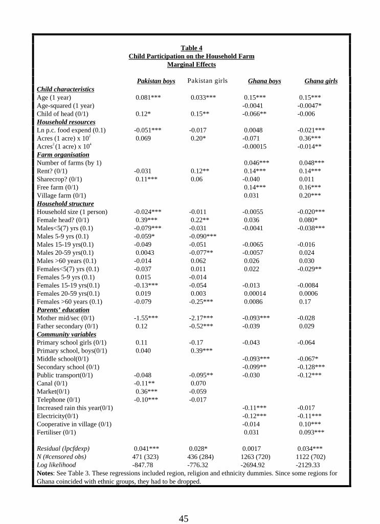
vector Z is household size (Table 3). Estimates of marginal effects for

a model with a larger set of control variables are presented in Tables 4

and 5 for the probability of working and for the hours of work

conditional on working respectively. The standard marginal effects

are multiplied by 0.1 for per capita food expenditure (Y) because this

is in logarithms and for household composition variables because

these are proportions and, as a result, the effects of a 10% change in

these variable can be directly read off the Table.

Identification of the Effect of Household Living Standards

Instruments for household consumption are community-level

variables10. The first stage regression explains 31% of the variation in

per capita food expenditure in Pakistan and 29% in Ghana, and the

instruments are jointly significant at 1% and 10% respectively. We

find that the results change significantly (and in the expected

direction) if we do not instrument (see Tables 3-5 and Sections 6.1,

6.2), underlining the importance of employing IV methods in

studying the impact of household income on child work. Since most

papers investigating child labour do not instrument household

income (see Section 2), their estimates will tend to carry upward

biases. The rest of this section presents the results, first for Ghana,

and then for Pakistan, where contrasts with Ghana are highlighted.

10 Instruments in Pakistan are the community-level average of household consumption, thepercentage of households that own land, the percentage that sharecrop, and indicator dummiesfor the presence of a railway line and electricity. In Ghana, we simply use dummies for amarket and for piped water since other available characteristics (road, post office, gratingmachine) had no explanatory power in the first-stage regression.

27

Further analysis and a summary are presented in the concluding

section.

6.1. Results for Ghana

Consider the parsimonious model in Table 3. Farm size has a

highly significant positive effect for both boys and girls, the effect for

girls being 50% larger than that for boys. Household per capita

consumption has an unexpectedly positive effect on child work, and

we are unable to reject its exogeneity. Boys from larger households

work significantly more while girls’ farm labour is independent of

household size.

Adding a range of control variables (Tables 4 and 5) makes a

dramatic difference to these results. The effects of farm size,

consumption and household size all become insignificant for boys.

For girls, a significant positive effect of farm size persists, and

household p.c. consumption and size both become negative and

significant. For girls, therefore, each of the three main variables takes

the sign predicted by theory once appropriate conditioning variables

are included. In the extended model, as in the parsimonious model,

we are unable to reject exogeneity of the consumption variable for

boys. However, the null of exogeneity is now clearly rejected for girls.

The rest of this section summarises the effects of the additional

variables in Tables 4 and 5. Child characteristics have broadly similar

effects for boys and girls. Child work increases with age at a

decreasing rate. A complete set of birth-order dummies was included

but their coefficients were poorly determined. They were therefore

replaced by a single indicator variable for whether the child in

28

question was the oldest child in the household. This too was

insignificant for both genders and since it is closely related to age, it

was dropped. The dummy indicating whether the child was the child

of the household head (as opposed to nephew, sibling, foster child, etc)

is negative for both genders and significant for boys.

Households in Ghana often own several plots of land, with

ownership often divided between men and women in a household

(e.g. Iversen, 2000). We find a strong positive effect of the number of

farms operated on hours of work, of similar magnitude for boys and

girls. Since this result obtains when controlling for acres of land

operated by the household, it suggests not a size effect but an effect

associated with the subdivision of land. This merits further micro-

level research. The mode of operation of land (sharecrop, rent etc)

matters.

Girls, but not boys exhibit significantly more hours of farm

work in female-headed households. Indeed, there are no effects of

household composition on boys’ work. A further significant effect,

restricted to girls, is that they work less in households with male or

female children under 7 years of age, that is, younger than

themselves.

The only significant effect of the parent education variables is

that the sons of mothers with secondary-level education work less. Since

this is at given levels of household living standards, it would appear

to reflect preferences rather than resources.

Dummies for the presence of primary, middle and secondary schools

in the cluster take the expected negative signs and the latter two are

29

significant for both genders11. Public transport in the village has a

negative effect that is restricted to girls. This is consistent with the

hypothesis that distance to school may deter the attendance of girls

more than it does that of boys. Electricity in the village reduces child

work significantly. The use of fertilizers increases child work,

significantly in the case of girls. Community leader’s responses to

whether rain in the year of the survey was heavier than in the

preceding year suggest a negative effect of rainfall on child labour,

significant for boys. Irrigation and tractors do not have significant

effects on child work, nor does the presence of a village bank. To

avoid clutter, these variables are not shown in the Table. The set of

community variables is jointly significant for both boys (χ217=34,

p>χ2=0.01) and girls (χ217=27.6, p>χ2=0.05).

The region dummies are jointly very significant and have larger

effects for girls (χ26=58 for boys and χ2

6=48 for girls, p>χ2=0 for both).

Religion has no systematic effect on boys’ work (χ22=2, p>χ2=0.37) but

Christian girls work significantly fewer hours on average than

Animist girls who work less than Muslim girls (χ22=5.3, p>χ2=0.07).

The dummies for ethnicity are insignificant for girls (χ25=3.2,

p>χ2=0.67). Boys of Ewe ethnicity are significantly less likely to work

(χ25=11.9, p>χ2=0.04).

6.2. Results for Pakistan

The parsimonious equations in Table 3 show a positive effect of

11 The significance of cluster-specific (or community) variables in determining child work inGhana is substantially altered once standard errors are robust and cluster-adjusted. Allequations report the correct (adjusted) standard errors.

30

farm size on girls’ work but the positive coefficient estimated for boys

is insignificant. Household consumption has the expected negative

effect on child work but this is only significant for boys. For both boys

and girls, hours of work fall significantly with household size. Weak

exogeneity of the consumption variable is rejected for both genders in

Pakistan. Replacing IV with standard tobit estimation results in

consumption being completely insignificant for both boys and girls.

This is consistent with the expected sign of the simultaneity bias.

When additional regressors are included (Tables 4 and 5), all of

these effects persist except for the effect of household size on girls’

work, which becomes insignificant. Across both genders, the

significant coefficients take signs consistent with our theoretical

framework. Further consideration of the gender difference in the

results is deferred to Section 7. The rest of this section considers the

effects of the additional variables.

Child age has a positive effect on hours worked, which is much

larger for boys than for girls. There are no birth order effects. In

contrast to Ghana, children of the household head in Pakistan are more

likely than other children in the household to be at work on the farm.

As in Ghana, the mode of operation of land impacts on child labour for

a given size of farm.

The children of female-headed households in Pakistan work

significantly more and the effect is bigger for boys than for girls. In

Ghana this effect was restricted to girls. These results suggest that

there are aspects of illbeing or insecurity in female headed

households that household consumption and farm size do not pick

up. Controlling for household size, there are some fairly complex

31

effects of the age-gender composition of the household on child work in

Pakistan, in contrast with Ghana where these effects were limited.

Both boys and girls in Pakistan work less if they have young siblings.

We found a similar effect for Ghanaian girls. This contradicts

evidence from other regions which finds that children - and especially

girls - with more siblings work longer hours on average (see Lloyd

(1993) and Jomo (1992)). In addition, girls in Pakistan work

significantly less in households with a relatively high fraction of adult

men and elderly women. Boys work less in households with a high

fraction of 15-19 year-old girls.

There is a significant negative effect of fathers’secondary

education that is restricted to girls. Mothers’ education to the level of

middle or secondary school has a huge negative effect on child work

for both genders, in contrast to Ghana where mothers education

reduces the work of boys but not girls.

The presence in the cluster of a primary school for girls reduces

the farm labour of girls and, possibly because of sibling competition

for resources, the presence of a primary school for boys increases

girls’ farm labour. These school-access variables have no effect on

boys’ work. The presence of a bus route (public transport) has a

negative effect on girls’ work, just as in Ghana. Cluster specific

variables which have a significant effect on boys’ work include

positive effects from a market and negative effects from a telephone and

a canal. For girls, community-level variables are altogether less

significant than for boys. The cluster-level variables are jointly

significant at the 10% level for boys (χ211=18.2, p>χ2=0.08) and

insignificant for girls (χ211=15.3, p>χ2=0.18).

32

Province dummies (χ23=11.7, p>χ2=0.0) and religion dummies

(χ22=17.9, p>χ2=0.0) are jointly significant for girls though not for boys

(χ23=4.5 χ2

2=2.9, respectively). Amongst girls, Christians work

significantly less than Muslims who work significantly less than other

Non-Muslims. The tendency for Christian girls to work relatively less

was also seen for Ghana. Christians constitute 1.5% of the population

and other non-Muslims (mostly Hindus) account for another 3.6%;

the vast majority are Muslim.

6. Conclusions and Policy Implications

Comparative work is useful in investigating whether there are

behavioural patterns relating to child work. While South Asia has the

largest number of working children, Sub-Saharan Africa has the

highest incidence of child labour. Even though it claims the majority

of child workers, the agricultural work of children is severely

understudied as compared with the more visible forms of work in

Latin America and Asia which involve children in labour-intensive

manufacturing. The results of the paper are interesting not only with

regard to similarities and differences between Pakistan and Ghana

but also with regard to gender differences. These are briefly

summarised in this section.

Controlling for household consumption, we identify a positive

effect of farm size on girls’ work in both countries, and no significant

association for boys. This suggests that the substitution effect is larger

for girls than for boys, which is consistent with the finding in a range

of developed country data sets that female labour supply is more

33

elastic than male labour supply. It also coincides with the finding that

the substitution effect is larger for girls than for boys in the supply of

wage labour in Pakistan (see Bhalotra, 1998).

There are significant effects of land tenure type (mode of

operation) on child labour at given acreage. No other study of child

labour has considered this factor at either the theoretical or the

empirical level.

We observe a negative relation of child work and household

food consumption per capita (our proxy for income) for boys in

Pakistan and girls in Ghana, the marginal effect being much larger in

the former case. In Pakistan, an increase in per capita food

expenditure of 10% is estimated to reduce the probability of boys’

work by 5 percentage points (so that, at the mean, the observed

participation rate of 32% would fall to 26%) and, conditional on

working, the same change in expenditure is expected to reduce hours

of work by 1.28 per week. The corresponding effects for girls in

Ghana are 2 percentage points and 0.31 hours per week. For

comparison with existing empirical work on child labour, it is worth

emphasising that we would find weaker income effects if we did not

account for simultaneity bias. Section 2 listed reasons why the

existing literature may not have identified a positive relation of

household poverty and child work, and the potential problems noted

there were avoided by careful specification. We nevertheless find no

income effect for the other two of the four groups of children in our

sample.

Consider possible reasons for the country and gender pattern of

the income elasticity. The absence of a negative income effect on the

34

work of boys in Ghana may be related to the fact that 75% of these

boys combine work and school (Table 1). In Pakistan, the absence of

an income effect on girls’ work is consistent with parents valuing a

son’s education over that of their daughters. The demand for girls’

schooling may be low because of low returns rather than because of

household income12. It may also be relevant that boys work

considerably longer hours than girls on average (Table 2).

It is useful to affirm the plausibility of our results by looking

back to the raw data organised by income group. Table 6 presents

activity rates and average work hours for children by income quartile.

It is only for Pakistani boys that participation rates in farm work

decline monotonically with household living standards. The

descriptive data are therefore consistent with the tobit estimates of

the income effect13. Note also that a stronger negative relation of

expenditure and child work is observed in the case of wage work

(Panel 2, Table 6). School attendance increases steadily with income in

Pakistan but does not exhibit a clear income effect in Ghana (Panel 3).

The results obtain upon holding constant region, religion and

ethnicity of the household as well as a variety of community

characteristics which, amongst other things, are expected to control

for demand effects. There is some evidence that access to school

affects child labour, especially in Ghana. An interesing finding is that

the presence of public transport in the village has a negative effect

that is restricted to girls. The negative effect of the presence of a canal

12 Bhalotra (2000) finds higher returns to school for men than for women in rural Pakistan and,in contrast, Glewwe (2000) finds that the return to school for women in Ghana is no lower thanthe return for men.13 The negative income effect for girls in Ghana did not appear in the parsimonious model inTable 3, showing that its identification relies upon introducing the set of controls in Tables 4-5

35

on boys’ work in Pakistan and the negative effect of increased rainfall

on boys’ work in Ghana may indicate the power of interventions that

minimise income fluctuations in reducing child labour.

We find that children from larger households are not more

likely to work or to work harder. Female headship significantly

increases child labour in every case except for that of boys in Ghana.

The size of this effect is much larger in Pakistan than in Ghana, where

the proportion of female-headed households is enormously larger

(30% as compared with less than 3%). There are some interesting and

large effects of the age-gender composition of the household in

Pakistan, though the corresponding effects in Ghana are weak.

Father’s secondary education significantly reduces girls’ work in

Pakistan but has no effect on the labour of the other three groups.

Mother’s secondary education tends to reduce child hours of work in

both countries. In Ghana this effect is restricted to boys but in

Pakistan it is significant for boys and girls, and of similar magnitude.

These findings reinforce a growing literature on the importance of

female education in achieving positive outcomes for children across a

range of countries. The magnitude of the effects we find is so large

that policy aimed at eliminating child work is best targeted here.

36

References

Ainsworth, Martha, 1996, Economic aspects of child fostering inCote d’Ivoire, Research in Population Economics, Volume 8, 25-62.

Altonji, J.G., 1983, Intertemporal substitution in labour supply:Evidence from micro-data, Journal of Political Economy.

Bardhan, P. and C. Udry, 1999, Development Microeconomics,Oxford University Press.

Basu, Kaushik and Van, P.(1998), The Economics of ChildLabor, American Economic Review, June.

Basu, Kaushik, 1997, Analytical Development Economics:The LessDeveloped Economy Revisited, MIT Press.

Basu, Kaushik, 1999, The intriguing relation between the adultminimum wage and child labour. Mimeograph, Cornell University.

Benjamin, Dwayne, 1992, Household composition, labourmarkets and labour demand: Testing for separation in agriculturalhousehold models, Econometrica, 60(2): 287-322.

Bekombo, M. (1981), The child in Africa: socialization,education and work, Chapter 4 in G. Rodgers and G. Standing (eds.),Child Work, Poverty and Underdevelopment, Geneva: ILO.

Bhalotra, S.R., 1998, Is child work necessary?, Mimeograph,University of Cambridge.

Bhalotra, S.R., 2000, Are the parents of working childrenselfish?, Mimeograph, University of Cambridge.

Bhalotra, S.R., 2000, Gender differences in returns to school inrural Pakistan, Mimeograph, University of Cambridge.

Bhalotra, S.R. and C.J. Heady, 2000, Child activities in SouthAsia and Sub-Saharan Africa: A comparative analysis, in: P. Lawrenceand C. Thirtle, eds., Africa and Asia in Comparative Development,(London: Macmillan), forthcoming.

37

Blinder, A.S. and Y. Weiss, 1976, “Human capital and laborsupply: a synthesis”, Journal of Political Economy, Vol. 84, 449-472.

Blunch, N-H and D. Verner, 2000, The child labour-poverty linkrevisited: The case of Ghana, Mimeograph, The World Bank.

Butcher, Kristin and Anne Case, 1994, The effect of sibling sexcomposition on women’s education and earnings, Quarterly Journal ofEconomics, 109(3), pp. 531-563.

Cain, Mead T., 1977, The economic activities of children in avillage in Bangladesh, Population and Development Review, vol. 3(3),201-27.

Canagarajah, Sudarshan and Coulombe, Harry 1998, Childlabor and schooling in Ghana, mimeograph, World Bank.

Cigno, A., F. Rosati and Z. Tzannatos, 1999, Child labor,nutrition and education in rural India: An economic analysis ofparental choice and policy options, Paper presented at the WorldBank Conference on Child Labour, Washington DC, April 11-13, 2000.

Cochrane, S., V. Kozel and H. Alderman, 1990, Householdconsequences of high fertility in Pakistan, World Bank DiscussionPaper No. 111, Washington DC.

Cockburn, John, 2000, Child labour in Ethiopia: Opportunitiesor income constraints?, Paper presented at a Conference onOpportunities in Africa: Microeconomic Evidence from Householdsand Firms, Oxford, April.

Das Gupta, Monica, 1987, Selective discrimination againstfemale children in rural Punjab, India, Population and DevelopmentReview, 13(1), 77-100.

Deaton, Angus, 1997, The Analysis of Household Surveys: TheMicroeconometrics of Household Surveys, The World Bank.

Driffill, E.J., 1980, “Life-cycles with terminal retirement”,International Economic Review, Vol. 21, No. 1, 45-62.

38

Eswaran, Mukesh, 1996, Fertility, literacy and the institution ofchild labor, Mimeograph, University of British Columbia, Vancouver.

Galasso, Emanuela, 1999, Intrahousehold allocation and childlabor in Indonesia, Department of Economics, Boston College,Mimeograph.

Glewwe, Paul, 1996, The relevance of standard estimates ofrates of return to schooling for education policy: A criticalassessment, Journal of Development Economics, Vol.51, pp.267-290

Grootaert, Christian, 1998, Child labour in Cote d’Ivoire:Incidence and determinants, Discussion Paper, Social DevelopmentDepartment, The World Bank, Washington D.C.

Grootaert, Christiaan and Harry Anthony Patrinos (1998), ThePolicy Analysis of Child Labor: A Comparative Study, The World Bank.

Heady, Chris, 1999, The effects of child work on educationalachievment, forthcoming as Discussion Paper, UNICEF InternationalChild Development Centre, Florence.

International Labor Organisation, 1996, Child Labour Today:Facts and Figures, Geneva: ILO.

Iversen, V. 2000, Child labour in a bargaining, agriculturalhousehold in sub-Saharan Africa, mimeograph, Wolfson College,University of Cambridge.

Jensen, Peter and Helena Skyt Nielsen (1997), Child labour orschool attendance? Evidence from Zambia, Journal of PopulationEconomics, 10, pp. 407-424.

Jensen, Robert T., 1999, Patterns, causes and consequences ofchild labor in Pakistan, Preliminary draft, John F. Kennedy School ofGovernment and Center for International Development, HarvardUniversity.

Jomo, K.S. (ed.), 1992, Child labor in Malaysia, Kuala Lumpur:Varlin Press.

Kanbargi, R. and P.M. Kulkarni, 1995, The demand for child

39

labour and child schooling in rural Karanataka, India, Mimeograph,Institute of Social and Economic Change, Bangalore, India.

Kassouf, A.L., 1998, Child labour in Brazil, Mimeograph,London School of Economics & University of Sao Paulo.

Killingsworth, M.R., 1982, “‘Learning by doing’ and ‘investmentin training’: a synthesis of two ‘rival’ models of the life cycle”, Reviewof Economic Studies, Vol. 49, 263-271.

Killingsworth, M.R., 1983, Labor Supply, Cambridge: CambridgeUniversity Press.

Lahiri, Sajal and S. Jaffrey (1999), Will trade sanctions reducechild labour?: The role of credit markets, Mimeograph, Departmentof Economics, University of Essex.

Ranjan, Priya (1999), An economic analysis of child labor,Economics Letters, 64, 99-105.

Lloyd, C.B., 1993, Fertility, family size and structure-consequences for families and children, Proceedings of a PopulationCouncil seminar, New York, 9-10 June, 1992, New York: ThePopulation Council.

McElroy, M., 1990, Nash-bargained household decisions- Reply,International Economic Review, 31(1):237-242.

Patrinos, H. and G. Psacharapoulos, 1997, “Family size,schooling and child labor in Peru - An empirical analysis”, Journal ofPopulation Economics, Vol. 10, 387-405.

Psacharapoulos, G., 1997, “Child labor versus educationalattainment: Some evidence from Latin America”, Journal of PopulationEconomics, Vol. 10 (4), 1-10.

Ravallion, Martin and Quentin Wodon (2000), Does child labourdisplace schooling? Evidence on behavioural responses to anenrolment subsidy, The Economic Journal, vol. 110, pp.c158-c175.

Ray, Ranjan (2000), Analysis of child labour in Peru andPakistan: A comparative study, forthcoming in Journal of Population

40

Economics.

Rosenzweig, M. and R. Evenson, 1977, Fertility, schooling andthe economic contribution of children in rural India: An econometricanalysis, Econometrica, 45(5):1065-1079.

Singh, R.D. and G.E.Schuh, 1986, The economic contribution offarm children and household fertility decisions: Evidence from adeveloping country, Brazil, Indian Journal of Agricultural Economics,41(1), 29-41.

Smith, R.J. and R. Blundell, 1986, An exogeneity test for thesimultaneous equation tobit model, Econometrica, 54, 679-85.

Strauss, John, 1986, in Singh, I., L. Squire and J. Strauss, Eds.(1986). AgriculturalHousehold Models: Extensions, Application and Policy. Baltimore (Md.),Johns Hopkins University Press.

Townsend, Robert, 1994, Risk and insurance in village India,Econometrica, May, 62, 539-92.

U.S. Department of Labour, 2000, By the sweat and toil ofchildren (vol.VI): An economic consideration of child labor,Washington DC: U.S. Department of Labour, Bureau of InternationalLabor Affairs.

White, H., 1980, A heteroskedasticity-consistent covariancematrix estimator and a direct test for heteroskedasticity, Econometrica48: 817-30.

41

Table 1

Child Activities

Pakistan

boys

Pakistan

Girls

Ghana

Boys

Ghana

Girls

Total participation rates

Household Farm work 22.1% 28.1% 40.5% 34.4%

Household Enterprise work 2.3% 1.6% 1.8% 2.5%

Wage work 6.2% 11.9% 0% 0%

School 72.8% 30.5% 76.5% 68.9%

None of the above activities 14.0% 42.4% 12.7% 20.1%

Domestic work n.a. 99.4% 89.8% 96.2%

Participation in one

activity

Farm work only 8.6% 21.1% 10.6% 9.8%

Enterprise work only 0.64% 1.2% 0.3% 1.2%

Wage work only 3.2% 6.8% 0% 0%

School only 61.3% 27.6% 45.0% 43.3%

Combinations of types of work

Farm & enterprise work 0.91% 0.09% 0% 0%

Hh farm & wage work 2.1% 4.1% 0% 0%

Hh enterprise & wage work 0.25% 0.27% 0% 0%

Combination of work & school

Farm work & school 10.5% 2.7% 29.9% 24.6%

Enterprise work & school 0.50% 0% 1.5% 1.3%

Wage work & school 0.74% 0.73% 0% 0%

Number of children 1209 1096 1718 1542

Notes: Rural areas. Ghana: 7-14 year-olds, Pakistan: 10-14 year-olds.

42

Table 2

Weekly Hours of Child Farm Work

Household farm Wage work

Ghana boys 15.5 (13.3)

N=696

Ghana girls 15.4 (12.9)

N=531

Pakistan boys 22.5 (18.5)

N=267

44.9 (22.3)

N=61

Pakistan girls 13.3 (13.8)

N=308

30.9 (15.6)

N=73

Notes: Hours are values reported for the reference week, conditional on

participation in the activity in the reference week. Girls’ participation has a

large seasonal component and so not all participating girls participate in the

week before the survey. Figures in parentheses are standard deviations around

the means. N is the number of observations (or the number of working children).

For Ghana the data refer to 7-14 year olds and for Pakistan to 10-14 year olds.

43

Table 3

Child Work on the Household Farm: Parsimonious Model

Marginal Effects

Pakistan boys Pakistan

girls

Ghana boys Ghana girls

Participation

Probabilities

Log p.c. food expend (0.1) -0.026*** -0.010 0.012*** 0.0095**

Acres (1 acre) x 102 0.026 0.15** 0.41*** 0.60***

Acres2 (1 acre) x 104 -0.31* -0.30

Household size (1 person) -0.021*** -0.013*** 0.0098*** -0.0069

Residual (lpcfdexp) 0.022*** 0.017** -0.006 -0.000053

Hours Conditional on Work

Log p.c. food expend (0.1) -0.68*** -0.18 0.22*** 0.16**

Acres (1 acre) x 102 0.68 2.70** 7.40*** 10.20***

Acres2 (1 acre) x 104 -5.50* -5.10

Household size (1 person) -0.54*** -0.25*** 0.18*** -0.12

Residual (lpcfdexp) 0.59*** 0.030** -0.11 -0.0009

N513 473 1272 1127

Log likelihood -969.82 -901.27 -2895.3 -2278.3

44

Notes: Figures are marginal effects at sample means for the change indicated in parentheses in column

1. Based on tobit estimates with Dependent variable: hours worked by children on the household farm.

Sample: Rural households that operate some land. ***, ** and * denote significance at the 5%, 10%

and 12% levels respectively. The regressions included region, religion and ethnicity dummies. Since

some regions for Ghana coincided with ethnic groups, they had to be dropped. Variables that were

insignificant in all four samples are not shown.

45

Table 4Child Participation on the Household Farm

Marginal Effects

Pakistan boys Pakistan girls Ghana boys Ghana girlsChild characteristicsAge (1 year) 0.081*** 0.033*** 0.15*** 0.15***Age-squared (1 year) -0.0041 -0.0047*Child of head (0/1) 0.12* 0.15** -0.066** -0.006Household resourcesLn p.c. food expend (0.1) -0.051*** -0.017 0.0048 -0.021***Acres (1 acre) x 102 0.069 0.20* -0.071 0.36***Acres2 (1 acre) x 104 -0.00015 -0.014**Farm organisationNumber of farms (by 1) 0.046*** 0.048***Rent? (0/1) -0.031 0.12** 0.14*** 0.14***Sharecrop? (0/1) 0.11*** 0.06 -0.040 0.011Free farm (0/1) 0.14*** 0.16***Village farm (0/1) 0.031 0.20***Household structureHousehold size (1 person) -0.024*** -0.011 -0.0055 -0.020***Female head? (0/1) 0.39*** 0.22** 0.036 0.080*Males<5(7) yrs (0.1) -0.079*** -0.031 -0.0041 -0.038***Males 5-9 yrs (0.1) -0.059* -0.090***Males 15-19 yrs(0.1) -0.049 -0.051 -0.0065 -0.016Males 20-59 yrs(0.1) 0.0043 -0.077** -0.0057 0.024Males >60 years (0.1) -0.014 0.062 0.026 0.030Females<5(7) yrs (0.1) -0.037 0.011 0.022 -0.029**Females 5-9 yrs (0.1) 0.015 -0.014Females 15-19 yrs(0.1) -0.13*** -0.054 -0.013 -0.0084Females 20-59 yrs(0.1) 0.019 0.003 0.00014 0.0006Females >60 years (0.1) -0.079 -0.25*** 0.0086 0.17Parents’ educationMother mid/sec (0/1) -1.55*** -2.17*** -0.093*** -0.028Father secondary (0/1) 0.12 -0.52*** -0.039 0.029Community variablesPrimary school girls (0/1) 0.11 -0.17 -0.043 -0.064Primary school, boys(0/1) 0.040 0.39***Middle school(0/1) -0.093*** -0.067*Secondary school (0/1) -0.099** -0.128***Public transport(0/1) -0.048 -0.095** -0.030 -0.12***Canal (0/1) -0.11** 0.070Market(0/1) 0.36*** -0.059Telephone (0/1) -0.10*** -0.017Increased rain this year(0/1) -0.11*** -0.017Electricity(0/1) -0.12*** -0.11***Cooperative in village (0/1) -0.014 0.10***Fertiliser (0/1) 0.031 0.093***

Residual (lpcfdexp) 0.041*** 0.028* 0.0017 0.034***N (#censored obs) 471 (323) 436 (284) 1263 (720) 1122 (702)Log likelihood -847.78 -776.32 -2694.92 -2129.33Notes: See Table 3. These regressions included region, religion and ethnicity dummies. Since some regions forGhana coincided with ethnic groups, they had to be dropped.

46

Table 5Hours of Child Farm Work Conditional on Participation

Marginal Effects

Pakistan Boys Pakistan Girls Ghana Boys Ghana GirlsChild characteristicsAge (1 year) 1.86*** 0.46*** 2.33*** 2.25***Age-squared (1 year) -0.063 -0.069*Child of head (0/1) 2.70* 2.09** -1.02** -0.083Household resourcesLn p.c. food expend (0.1) -1.16*** -0.24 0.073 -0.31**Acres (1 acre) x 102 1.60 2.90* 1.10 5.40***Acres2 (1 acre) x 104 -0.0024 -0.20**Farm organisationNumber of farms (by 1) 0.71*** 0.70***Rent (0/1) -0.70 1.74** 2.09*** 2.14***Sharecrop (0/1) 2.62*** 0.78 -0.62 0.15Free farm (0/1) 2.22*** 2.32***Village farm(0/1) 0.47 2.96***Household structureHousehold size (by 1) -0.54*** -0.16 -0.085 -0.30***Female head? (0/1) 9.02*** 3.06** 0.55 1.18*Males <5(7) years (0.1) -1.8*** -0.44 0.063 -0.56***Males 5-9 years(0.1) -1.35* -1.27***Males 15-19 years(0.1) -1.11 -0.71 -0.10 -0.24Males 20-59 years(0.1) -0.098 -1.09** 0.088 0.36Males >60 years (0.1) -0.32 0.88 0.39 0.44Females<5(7) yrs (0.1) -0.86 0.16 0.34 -0.43**Females 5-9 yrs (0.1) 0.35 -0.20Females 15-19 yrs(0.1) -2.86*** -0.76 -0.20 -0.12Females 20-59 yrs(0.1) 0.43 0.045 0.0021 0.0096Females over 60 yrs(0.1) -1.81 -3.53*** 0.13 0.25Parents’ education(0/1)Mother mid/sec (0/1) -35.45*** -30.58*** -1.43*** -0.41Father secondary (0/1) 2.75 -7.26*** -0.6 0.43Community variablesPrimary school girls (0/1) 2.43 -2.41 -0.67 -0.94Primary school, boys(0/1) 0.90 5.43***Middle school(0/1) -1.43*** -0.98*Secondary school (0/1) -1.53** -1.88***Public transport(0/1) -1.11 -1.34** -0.46 -1.72***Canal (0/1) -2.45** 0.97Market(0/1) 8.14*** -0.82Telephone (0/1) -2.32*** -0.24Increased rain this year(0/1) -1.69*** -0.24Electricity(0/1) -1.86*** -1.54***Cooperative in village (0/1) -0.21 1.51***Fertiliser (0/1) 0.48 1.37***

Residual (lpcfdexp) 0.95*** 0.40* 0.027 0.49***N (#censored obs) 471(323) 436(284) 1263(720) 1122(702)Log likelihood -847.78 -776.32 -2694.92 -2129.33Notes: See Notes to Table 3.

47

Table 6Child Activities By Quartile of Per Capita Food Expenditure

Pakistan boys Pakistan girls Ghana boys Ghanagirls

Hh Farm Work

Full sample 22.1(23.3)

28.1(13.3)

40.5(15.5)

34.4(15.4)

Quartile 1 24.3(20.6)

25.4(11.5)

36.7(18)

30.4(13)

Quartile 2 23.0(23.2)

26.8(15.3)

37.7(14)

29.3(14)

Quartile 3 21.1(25.2)

29.7(13.9)

44.1(15)

39.3(17)

Quartile 4 19.8(25.1)

30.8(12.6)

43.8(15)

38.6(17)

Wage Work

Full sample 6.2(31)

11.9(45)

Quartile 1 8.2(44.6)

18.8(31.7)

Quartile 2 6.9(51.8)

11.5(33.6)

Quartile 3 4.7(40.7)

8.0(35.5)

Quartile 4 5.0(36.4)

9.4(24.7)

School Attendance

Full sample 72.8 30.5 76.5 68.9Quartile 1 65.4 26.3 70.0 61.3Quartile 2 69.3 26.8 79.6 74.7Quartile 3 77.0 33.5 75.6 69.2Quartile 4 79.1 36.0 81.4 69.4

Notes: See Notes to Tables 1-3. Hh=household. All figures are percentages except figures inparentheses which are weekly hours of work in the reference week, conditional on participation.

48

Appendix Table 1Variable Means for Workers and Non-Workers by Gender

Rural Ghana

Boys in Ghana Girls in GhanaWorkers Non-workers Workers Non-workers

#Observations 687 884 523 884

Dependent variablehours worked on farm 15.5 0 15.5 0Child characteristicsage 10.9 9.8 10.9 9.7first child 0.61 0.47 0.64 0.48child of head of hh 0.77 0.84 0.72 0.81Household resourcesln pc food expenditure -0.33 -0.40 -0.27 -0.39acres of land 9.34 8.23 9.77 7.57Size of farmnumber of farms 2.0 1.94 2.1 1.92rent land? 0.086 0.055 0.071 0.083sharecrop land? 0.070 0.067 0.067 0.066freely available land? 0.23 0.15 0.21 0.15village-owned land? 0.23 0.26 0.24 0.28

Household structurehousehold size 7.3 7.2 6.9 7.3female head? 0.27 0.20 0.34 0.22males under 7 years 0.10 0.11 0.091 0.11males 7-14 years 0.28 0.28 0.10 0.095males 15-19 years 0.059 0.049 0.059 0.049males 20-59 years 0.10 0.11 0.11 0.11males over 60 years 0.033 0.032 0.032 0.028females under 7 yrs 0.098 0.097 0.097 0.103females 7-14 years 0.085 0.088 0.27 0.26females 15-19 years 0.041 0.034 0.037 0.039females 20-59 years 0.16 0.18 0.18 0.18females over 60 years 0.033 0.020 0.037 0.019

Parents’ educationmother none 0.68 0.66 0.66 0.69mother primary 0.15 0.11 0.13 0.14mother secondary 0.17 0.23 0.21 0.17father none 0.51 0.49 0.46 0.53father primary 0.086 0.088 0.079 0.085father secondary 0.40 0.42 0.46 0.38

Community variablesAccess to schoollocal primary school 0.85 0.89 0.87 0.88local middle school 0.61 0.64 0.70 0.63local secondary school 0.14 0.11 0.11 0.10local public transport 0.52 0.50 0.52 0.47Quality of schoolage of primary school 33.5 32.1 35.1 32.6age of middle school 15.1 10.1 15.1 11.6

49

age of sec/tech sch 16.1 17.1 15.9 18.0Farming technologyco-operative society 0.29 0.31 0.36 0.27mutual aid for workers 0.87 0.88 0.86 0.88irrigation 0.038 0.041 0.026 0.039increased rain this year 0.64 0.77 0.60 0.75husking machine 0.074 0.060 0.072 0.058fertilizer 0.56 0.58 0.57 0.54Economic infrastructureelectricity 0.12 0.14 0.15 0.17bank 0.094 0.084 0.14 0.076Dynamismlife better than 1981 0.27 0.23 0.32 0.26easier to find work 0.27 0.31 0.32 0.29RegionsCentral Region 0.14 0.083 0.15 0.10Eastern Region 0.028 0.25 0.027 0.21West 0.096 0.11 0.12 0.11Volta Region 0.14 0.088 0.14 0.081Ashanti Region 0.24 0.078 0.26 0.078Brong Ahafo Region 0.13 0.13 0.15 0.14North 0.08 0.11 0.05 0.12Upper West 0.04 0.04 0.03 0.05Upper East 0.08 0.10 0.08 0.11Ethnic groupsAkan 0.57 0.48 0.61 0.46Ewe 0.038 0.058 0.056 0.059Ga-adangbe 0.038 0.11 0.024 0.089Dagbani 0.054 0.041 0.028 0.049Nzema 0.013 0.013 0.015 0.017Other 0.29 0.30 0.26 0.32ReligionChristian 0.61 0.60 0.65 0.58Animist/traditional 0.19 0.25 0.16 0.25Muslim 0.20 0.15 0.19 0.17Notes: See Notes to Table 3. Not all community variables shown here are used in the analysis. Per capiexpenditure for Ghana is expressed as a ratio to its mean, not so for Pakistan. This makes no effective differencto the tobit estimates since the variable is in logarithms and there is an equation constant.

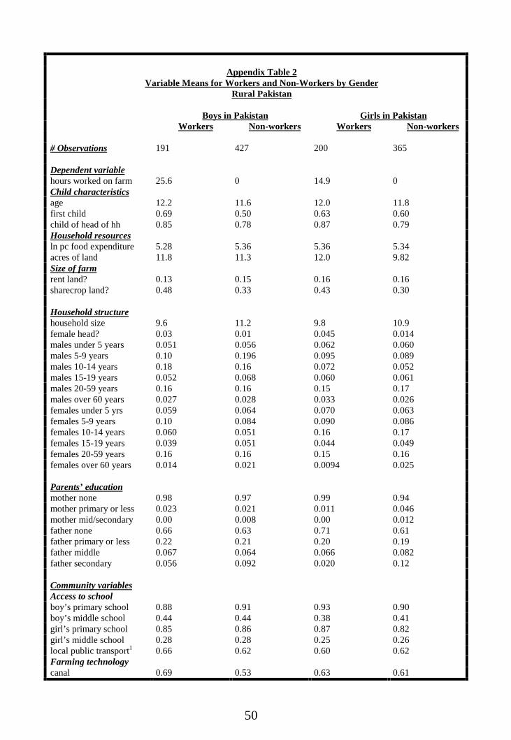
50

Appendix Table 2Variable Means for Workers and Non-Workers by Gender

Rural Pakistan

Boys in Pakistan Girls in PakistanWorkers Non-workers Workers Non-workers

# Observations 191 427 200 365

Dependent variablehours worked on farm 25.6 0 14.9 0Child characteristicsage 12.2 11.6 12.0 11.8first child 0.69 0.50 0.63 0.60child of head of hh 0.85 0.78 0.87 0.79Household resourcesln pc food expenditure 5.28 5.36 5.36 5.34acres of land 11.8 11.3 12.0 9.82Size of farmrent land? 0.13 0.15 0.16 0.16sharecrop land? 0.48 0.33 0.43 0.30

Household structurehousehold size 9.6 11.2 9.8 10.9female head? 0.03 0.01 0.045 0.014males under 5 years 0.051 0.056 0.062 0.060males 5-9 years 0.10 0.196 0.095 0.089males 10-14 years 0.18 0.16 0.072 0.052males 15-19 years 0.052 0.068 0.060 0.061males 20-59 years 0.16 0.16 0.15 0.17males over 60 years 0.027 0.028 0.033 0.026females under 5 yrs 0.059 0.064 0.070 0.063females 5-9 years 0.10 0.084 0.090 0.086females 10-14 years 0.060 0.051 0.16 0.17females 15-19 years 0.039 0.051 0.044 0.049females 20-59 years 0.16 0.16 0.15 0.16females over 60 years 0.014 0.021 0.0094 0.025

Parents’ educationmother none 0.98 0.97 0.99 0.94mother primary or less 0.023 0.021 0.011 0.046mother mid/secondary 0.00 0.008 0.00 0.012father none 0.66 0.63 0.71 0.61father primary or less 0.22 0.21 0.20 0.19father middle 0.067 0.064 0.066 0.082father secondary 0.056 0.092 0.020 0.12

Community variablesAccess to schoolboy’s primary school 0.88 0.91 0.93 0.90boy’s middle school 0.44 0.44 0.38 0.41girl’s primary school 0.85 0.86 0.87 0.82girl’s middle school 0.28 0.28 0.25 0.26local public transport1 0.66 0.62 0.60 0.62Farming technologycanal 0.69 0.53 0.63 0.61

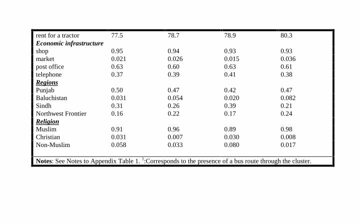
51

rent for a tractor 77.5 78.7 78.9 80.3Economic infrastructureshop 0.95 0.94 0.93 0.93market 0.021 0.026 0.015 0.036post office 0.63 0.60 0.63 0.61telephone 0.37 0.39 0.41 0.38RegionsPunjab 0.50 0.47 0.42 0.47Baluchistan 0.031 0.054 0.020 0.082Sindh 0.31 0.26 0.39 0.21Northwest Frontier 0.16 0.22 0.17 0.24ReligionMuslim 0.91 0.96 0.89 0.98Christian 0.031 0.007 0.030 0.008Non-Muslim 0.058 0.033 0.080 0.017

Notes: See Notes to Appendix Table 1. 1:Corresponds to the presence of a bus route through the cluster.