china and the manufacturing exports of other developing ... · pdf filechina and the...
TRANSCRIPT
NBER WORKING PAPER SERIES
CHINA AND THE MANUFACTURING EXPORTS OF OTHER DEVELOPING COUNTRIES
Gordon H. HansonRaymond Robertson
Working Paper 14497http://www.nber.org/papers/w14497
NATIONAL BUREAU OF ECONOMIC RESEARCH1050 Massachusetts Avenue
Cambridge, MA 02138November 2008
We thank Irene Brambilla, Ernesto Lopez Cordoba, Robert Feenstra, David Hummels, Daniel Lederman,Marcelo Olarreaga, Guillermo Perry, and Christian Volpe for helpful comments. The views expressedherein are those of the author(s) and do not necessarily reflect the views of the National Bureau ofEconomic Research.
NBER working papers are circulated for discussion and comment purposes. They have not been peer-reviewed or been subject to the review by the NBER Board of Directors that accompanies officialNBER publications.
© 2008 by Gordon H. Hanson and Raymond Robertson. All rights reserved. Short sections of text,not to exceed two paragraphs, may be quoted without explicit permission provided that full credit,including © notice, is given to the source.
China and the Manufacturing Exports of Other Developing CountriesGordon H. Hanson and Raymond RobertsonNBER Working Paper No. 14497November 2008JEL No. F15
ABSTRACT
In this paper, we examine the impact of China's growth on developing countries that specialize in manufacturing.Over 2000-2005, manufacturing accounted for 32% of China's GDP and 89% of its merchandise exports,making it more specialized in the sector than any other large developing economy. Using the gravitymodel of trade, we decompose bilateral trade into components associated with demand conditionsin importing countries, supply conditions in exporting countries, and bilateral trade costs. We identify10 developing economies for which manufacturing represents more than 75% of merchandise exports(Hungary, Malaysia, Mexico, Pakistan, the Philippines, Poland, Romania, Sri Lanka, Thailand, andTurkey), which are in theory the countries most exposed to the adverse consequences of China's exportgrowth. Our results suggest that had China's export supply capacity been constant over the 1995-2005period, demand for exports would have been 0.8% to 1.6% higher in the 10 countries studied. Thus,even for the developing countries most specialized in export manufacturing, China's expansion hasrepresented only a modest negative shock.
Gordon H. HansonIR/PS 0519University of California, San Diego9500 Gilman DriveLa Jolla, CA 92093-0519and [email protected]
Raymond RobertsonDepartment of EconomicsMacalester College1600 Grand AveSt. Paul MN [email protected]
1
1. Introduction
The explosive growth of China’s economy has been extraordinary. Between 1990 and
2005, China’s exports increased by 25 times in real terms, compared to an increase of about four
times in the 12 largest exporting nations (Table 1). As of 2005, China’s exports accounted for
25% of the total exports of all countries outside of the top 12.1
What has made China’s emergence potentially disruptive is that the country is highly
specialized in manufacturing. Over the period 2000 to 2005, manufacturing accounted for 32%
of China’s GDP and 89% of its merchandise exports, making it more specialized in the sector
than any other large developing economy (Table 2). In consumer goods and other labor-
intensive manufactures, China has become a major source of supply, pushing down world
product prices. Meanwhile, China has contributed to a boom in demand for commodities,
leading to increases in the prices of metals, minerals, and farm goods.
The impact of China’s emergence on other developing countries is just beginning to be
appreciated (Devlin, Estevadeordal, and Rodriguez-Clare, 2005; Eichengreen and Tong, 2005;
Lopez Cordoba, Micco, and Molina, 2005). In the 1980s and 1990s, international trade became
the engine of growth for much of the developing world. Trade liberalization and market-oriented
reform in Asia and Latin America steered the regions toward greater specialization in exports.
There is a popular conception that for non-oil-exporting developing countries expanding export
production has meant specializing in manufacturing. But in actuality there is considerable
heterogeneity in the production structures of these economies, which means there is variation in
national exposure to China’s industrial expansion.
1 This share excludes Hong Kong and Singapore, which are entrepot economies and whose exports contain a substantial share of re-exports.
2
Even excluding oil exporters and very poor countries, there are many countries that
specialize in primary commodities. In Chile, Cote d’Ivoire, Kenya, and Peru, for instance,
manufacturing accounts for less than 25% of merchandise exports (Table 2). One might expect
this group to have been most helped by China’s growth, with the commodity boom lifting their
terms of trade. Other countries have diversified export production, spanning agriculture, mining,
and manufacturing. In Argentina, Brazil, Colombia, Egypt, Indonesia, and Vietnam,
manufacturing accounts for 30% to 55% of merchandise exports. For this group, China may
represent a mixed blessing, increasing the prices of some of the goods they produce and
decreasing the prices of others. A third group of countries is highly specialized in
manufacturing. In Hungary, Mexico, Pakistan, the Philippines, and Turkey, manufacturing
accounts for more than 80% of merchandise exports. This last group includes the countries most
likely to be adversely affected by China, as it has become a rival source of supply in their
primary destination markets. Between 1993 and 2005, China’s share of total imports rose from
5% to 15% in the United States and from 4% to 12% in the European Union.
In this paper, we examine the impact of China’s growth on developing countries that
specialize in export manufacturing. Using the gravity model of trade, we decompose bilateral
trade into components associated with demand conditions in importing countries, supply
conditions in exporting countries, and bilateral trade costs. In theory, growth in China’s export-
supply capabilities would allow it to capture market share in the countries to which it exports its
output, possibly reducing demand for imports from other countries that also supply these
markets. We calculate the export demand shock that China’s growth has meant for other
developing countries, as implied by gravity model estimation results.
3
To isolate economies that are most exposed to China’s manufacturing exports, we select
developing countries that are also highly specialized in manufacturing. After dropping rich
countries, very poor countries, and small countries, we identify 10 medium-to-large developing
economies for which manufacturing represents more than 75% of merchandise exports:
Hungary, Malaysia, Mexico, Pakistan, the Philippines, Poland, Romania, Sri Lanka, Thailand,
and Turkey.2 This group includes a diverse set of countries in terms of geography and stage of
development, hopefully making our results broadly applicable. We focus on developing
countries specialized in manufacturing, as for this group the impact of China on their production
activities is largely captured by trade in manufactures. Manufacturing is also a sector for which
the gravity model is well suited theoretically.
In section 2, we use a standard monopolistic-competition model of trade to develop an
estimation framework. The specification is a regression of bilateral sectoral imports on importer
country dummies, exporter country dummies, and factors that affect trade costs (bilateral
distance, sharing a land border, sharing a common language, belonging to a free trade area, and
import tariffs). When these importer and exporter dummies are allowed to vary by sector and by
year, they can be interpreted as functions of structural parameters and country-specific variables
that determine a country’s export supply and import demand. Changes in import-demand
conditions can be decomposed into two parts, one of which captures changes in income levels in
import markets and another of which captures changes in sectoral import price indices for those
markets, which are themselves a function of other countries’ export-supply dummies.
In section 3, we report coefficient estimates based on our framework. The data for the
analysis come from the UN COMTRADE database and the TRAINS dataset, which cover the
2 In Table 2, it is apparent India would also satisfy our criteria. We exclude India because its recent growth represents another potentially important global economic shock for other developing countries.

4
period to 1995 to 2005. We estimate country-sector-year import dummies, country-sector-year
export dummies, and sector-year trade cost elasticities using data on a large set of trading
economies that account for much of world trade. We begin by reporting estimated sectoral
exporter dummy variables for the 10 developing-country exporters vis-à-vis China. For 9 of the
10 countries, export supply dummies are strongly positively correlated with China’s, suggesting
that their comparative advantage is relatively similar to that of China. The results also describe
how each country’s export-supply capacities have evolved over time. Relative to each of the 10
countries, the growth in China’s export supply capabilities has been dramatic.
The main results, presented in section 4, suggest that had China’s export-supply capacity
been constant over the 1995 to 2005 period, export demand would have been 0.6% to 1.8%
higher in the 10 countries studied. The impact is somewhat larger when excluding resource
intensive industries or when focusing on industries in which China’s revealed comparative
advantage appears to be strongest (apparel, footwear, electronics, toys). For developing
countries highly specialized in manufacturing, it appears China’s expansion has represented only
a modest negative shock.
It is important to note that our results do not represent a general equilibrium analysis of
China’s impact on other developing economies. China’s export growth may have increased the
number of product varieties available to these countries, thereby improving consumer welfare
(Broda and Weinstein, 2005), or had positive effects on the demand for non-manufacturing
output. Our approach does not account for changes in consumer welfare associated with changes
in product variety or non-manufacturing prices. Nevertheless, the results give a sense of the
extent to which China is in competition with other large developing country exporters for market
share abroad.
5
By way of conclusion, in section 5, we discuss what China’s continued growth may mean
for manufacturing-oriented developing countries.
2. Empirical Specification
Consider a standard monopolistic model of international trade, as in Anderson and van
Wincoop (2004) or Feenstra (2004). Let there be J countries and N manufacturing sectors,
where each sector consists of a large number of product varieties. All consumers have identical
Cobb-Douglas preferences over CES sectoral composites of product varieties, where in each sector
n there are In varieties of n produced, with country j producing Inj varieties. There are increasing
returns to scale in the production of each variety. In equilibrium each variety is produced by a
monopolistically-competitive firm and In is large, such that the price for each variety is a constant
markup over marginal cost. Free entry drives profits to zero, equating price with average cost.
Consider the variation in product prices across countries. We allow for iceberg transport
costs in shipping goods between countries and for import tariffs. The cost-including-freight (c.i.f.)
price of variety i in sector n produced by country j and sold in country k is then
nninjk nj nk jk
n
P = w t (d )1
γ⎛ ⎞σ⎜ ⎟σ −⎝ ⎠
, (1)
where Pinj is the free-on-board (f.o.b.) price of product i in sector n manufactured in country j; σn is
the constant elasticity of substitution between any pair of varieties in sector n; wnj is unit production
cost in sector n for exporter j; tnk is one plus the ad valorem tariff in importer k on imports of n
(assumed constant for all exporters that do not share a free trade area with importer k); djk is
distance between exporter j and importer k; and γn is the elasticity of transport costs with respect to
distance for goods in sector n.
6
Given the elements of the model, the total value of exports of goods in sector n by exporter j
to importer k can be written as,
1nk
1njknjknnjk
nn GPIYX −σσ−µ= , (2)
where µn is the expenditure share on sector n and Gnk is the price index for goods in sector n in
importer k. Equation (2) reduces to
( )1 nnn k nj nj njk jk
njk 1 nHnnh nh nhk hk
h 1
Y I w (d )X
I w (d )
−σγ
−σγ
=
µ τ=
⎡ ⎤τ∑ ⎣ ⎦
, (3)
which can be written in log form as
( ) ( ) ( )1k nnjk n nj n njk n n jknj1 nH
nnh nh nhk hkh 1
Yln X ln ln ln I w 1 ln 1 ln d
I w (d )
−σ−σ
γ
=
= µ + + + −σ τ + γ −σ⎡ ⎤τ∑ ⎣ ⎦
(3’)
Regrouping terms in (3’), and allowing for measurement error in trade values, we obtain
njk n nk nj 1n jk 2n jk njkln X m s ln ln d= θ + + +β τ +β + ε . (4)
In equation (4), we see that there are five sets of factors that affect country j’s exports to country k
in sector n. The first term ( n nlnθ = µ ) captures preference shifters specific to sector n; the second
term (1 nH
nnk k nh nh nhk hkh 1
m ln(Y / I w (d ) )−σ
γ
=⎡ ⎤= τ∑ ⎣ ⎦
) captures demand shifters in sector n and
importer k (which are a function of importer k’s income and supply shifters for other countries that
also export to k); the third term ( 1 nnj nj njs ln(I w )−σ= ) captures supply shifters in sector n for
exporter j (which reflect exporter j’s production costs and the number of varieties it produces in the
sector); the fourth and fifth terms (where 1n n1β = −σ and 2n n n(1 )β = γ −σ ) capture trade costs
7
specific to exporter j and importer k (which in the empirical analysis we measure using import
tariffs, bilateral distance, whether countries share a common language, whether countries share a
land border, and whether countries belong to a free trade area); and the final term ( njkε ) is a
residual. Exporter j’s shipments to importer k would expand if importer k’s income increases,
production costs increase or the number of varieties produced decreases in other countries that
supply importer k, exporter j’s supply capacity expands, or bilateral trade costs decrease.
Our first empirical exercise is to estimate equation (4). Then, we use the coefficient
estimates to examine the role of China in contributing to changes in import demand in other
countries. To motivate this approach, consider import-demand conditions in country k, as embodied
in the importer dummy variables in (4). In theory,
n n nH
1 1nk k nh nh nhk hk
h 1m ln Y ln I w d−σ −σ β
=
⎛ ⎞= − τ⎜ ⎟⎜ ⎟
⎝ ⎠∑ , (5)
which captures average expenditure per imported variety by country k in sector n. Import demand
conditions in k are a function of income in k, export supply conditions in k’s trading partners
(embodied in the number of varieties they produce and their production costs), and k’s bilateral
trade costs. Average expenditure per variety in country k would decrease if the number of varieties
produced globally increases (since a given sectoral expenditure level would be spread over more
varieties) or production costs in other countries increases (which would deflect expenditure away
from their varieties). Using (4), we can write (5) as,
1n 2nnhH ˆ ˆs
nk k nhk hkh 1
m ln Y ln e dβ β
=
⎛ ⎞= − τ⎜ ⎟⎜ ⎟
⎝ ⎠∑ , (6)
8
where nh 1n 2nˆ ˆs , , andβ β are OLS coefficient estimates from (4).3 Over time, import-demand
conditions in k will change as its income changes, its bilateral trade costs change, or export-supply
conditions in its trading partners change. As China’s export supply capacity in sector n improves
(due either to increases in the number of varieties it produces or decreases in its production costs),
average expenditure per imported variety in country k would fall, leading to a decrease in the
demand for imports from k’s trading partners.
Following this logic, we construct the implied change in demand for imports by country k
associated with changes in China’s export-supply capacity. Actual import demand conditions in
sector n for country k at time t are
1n 2n 1n 2nnht nctH ˆ ˆ ˆ ˆˆ ˆs s
nkt kt nhkt hk nckt ckh c
m ln Y ln e d e dβ β β β
≠
⎛ ⎞= − τ + τ⎜ ⎟⎜ ⎟
⎝ ⎠∑ , (7)
where c indexes China. Suppose China had experienced no growth in its export-supply capacity
between time 0 and time t. The counterfactual import-demand term for country k would then be
1n 2n 1n 2nnht nc0H ˆ ˆ ˆ ˆˆ ˆs s
nkt kt nhkt hk nckt ckh c
m ln Y ln e d e dβ β β β
≠
⎛ ⎞= − τ + τ⎜ ⎟⎜ ⎟
⎝ ⎠∑ . (8)
For each importing country in each sector, we calculate the value,
1n 2n 1n 2n 1n 2n 1n 2nnht nc0 nht nctH Hˆ ˆ ˆ ˆ ˆ ˆ ˆ ˆˆ ˆ ˆ ˆs s s s
nkt nkt nhkt hk nckt ck nhkt hk nckt ckh c h c
m m ln e d e d ln e d e dβ β β β β β β β
≠ ≠
⎡ ⎤⎛ ⎞ ⎛ ⎞− = − τ + τ − τ + τ⎢ ⎥⎜ ⎟ ⎜ ⎟⎜ ⎟ ⎜ ⎟⎢ ⎥⎝ ⎠ ⎝ ⎠⎣ ⎦
∑ ∑ ,
(9)
3 One might imagine estimating (4) subject to the constraint in (6). In practice, imposing such nonlinear constraints would greatly complicate the regression analysis. As a simple check on whether the constraints on the value of mnk appear to be satisfied in the data, we estimate equation (6) using OLS (after first estimating (4)), the results for which are reported in Table 4. In most specifications, the coefficient on log income ranges between 0.5 and 1.0 and the coefficient on the import price index (constructed from the coefficient estimates) is -0.3 to -0.5. These coefficient signs and magnitudes are roughly consistent with theory.
9
which shows the amount by which import demand in k would have differed at time t had China’s
export supply capacity remained unchanged between time 0 and time t.
We refer to the quantity in (9) as the counterfactual change in import demand in country k
and sector n. For each of the 10 developing country exporters, we calculate the weighted average of
(9) across importers and sectors. The resulting value is the difference in the demand for a country’s
exports implied by growth in China’s export-supply capacity. An exporter will be more exposed to
China’s growth the more its exports are concentrated in goods for which China’s export-supply
capacity has expanded and the more it trades with countries with which China has relatively low
trade costs. Obviously, this counterfactual exercise is not general-equilibrium in nature, and should
be interpreted with caution. Still, it may be useful for gauging which export producers have been
more exposed to export competition from China.
One problem with estimating (4) is that at the sectoral level there is zero trade between
many country pairs.4 Tenreyro and Santos Silva (2005) propose a Poisson pseudo-maximum
likelihood (PML) estimator to deal with zero observations in the gravity model. In our application,
this approach is subject to an incidental-parameters problem (Wooldridge, 2002). While in a
Poisson model it is straightforward to control for the presence of unobserved fixed effects, it is
difficult in this and many other nonlinear settings to obtain consistent estimates of these effects.
Since, at the sectoral level, most exporters trade with no more than a few dozen countries, PML
estimates of exporter and importer country dummies may be inconsistent.
Our approach is to estimate (4) using OLS for a set of medium to large exporters (OECD
countries plus larger developing countries, which together account for approximately 90% of world
manufacturing exports) and medium to large importers (which together account for approximately
90% of world manufacturing imports). For bilateral trade between larger countries, there are 4 Zero bilateral trade values further complicate estimating (4) subject to the constraint in (6).
10
relatively few zero trade values. Since we do not account explicitly for zero bilateral trade in the
data, we are left with unresolved concerns about the consistency of the parameter estimates, which
the trade literature has only recently begun to address.5
3. Gravity Estimation Results
The trade data for the analysis come from the UN COMTRADE database and cover
manufacturing imports over the period 1995 to 2005. We examine bilateral trade at the four-
digit harmonized system (HS) level for the union of the 40 largest manufacturing export
industries in each of the 10 developing-country exporters.6 The 40 industries account for the
majority of manufacturing exports in the 10 manufacturing exporters, ranging from 71% to 90%
for 7 of the 10 countries (the Philippines, Mexico, Turkey, Malaysia, Romania, Sri Lanka,
Pakistan) and from 48% to 62% in the 3 others (Hungary, Poland, Thailand). The tariff data,
which are based on Robertson (2007), come from the TRAINS database and are the simple
averages of available tariffs at the 10-digit HS level within each four-digit industry. We use the
tariffs that are most applicable to each sector-country pair. For some country pairs, these are the
importer’s MFN tariffs, for other pairs (e.g., NAFTA members) it is tariffs governed by a
regional trade agreement, and for others (e.g., U.S.-Israel) it is tariffs governed by a bilateral
trade agreement.7
We estimate the gravity equation in (4) on a year-by-year basis, allowing coefficients on
exporter country dummies, importer country dummies, and trade costs to vary by sector and
year. The output from the regression exercise is for each sector a panel of exporter and importer
country dummy variables, trade-cost coefficients, intercepts, and residuals. The country-sector
5 See Helpman, Melitz, and Rubinstein (2007). 6 Choosing a subset of industries helps keep the dimension of the estimation manageable. 7 We replace missing tariff data with interpolated values based on non-missing tariff data. See Robertson (2007).
11
dummies are the deviation from U.S. sectoral mean trade by year (as the U.S. in the excluded
country in all regressions). For these coefficients to be comparable across time, the conditioning
set for a given sector (i.e., the set of comparison countries) must be constant. For each sector, we
limit the sample to bilateral trading partners that have positive trade in every year during the
sample period.8
3.1 Summary of Coefficient Estimates
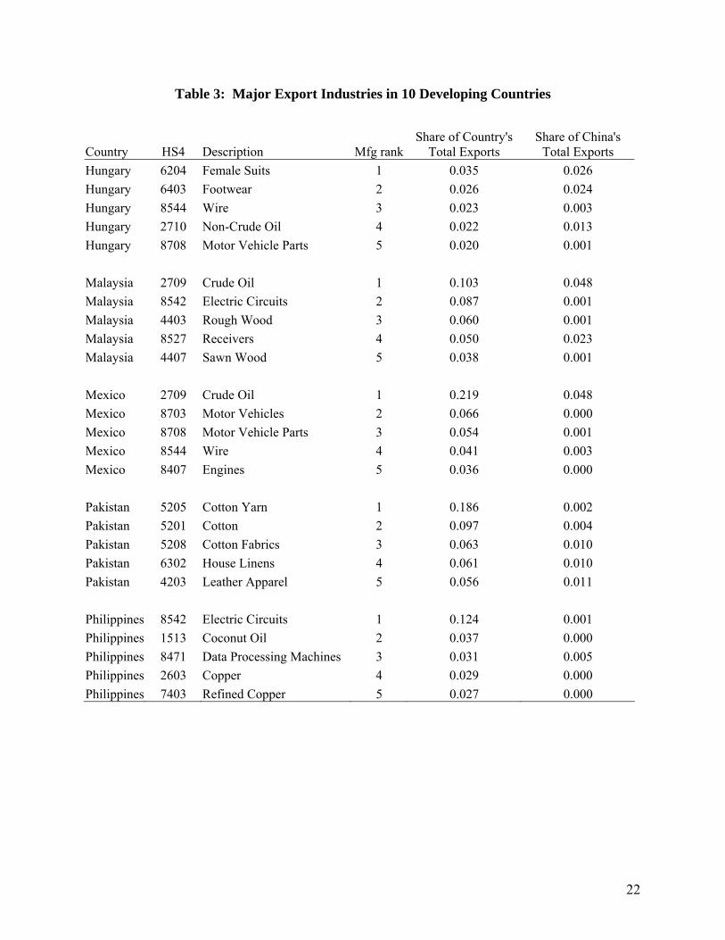
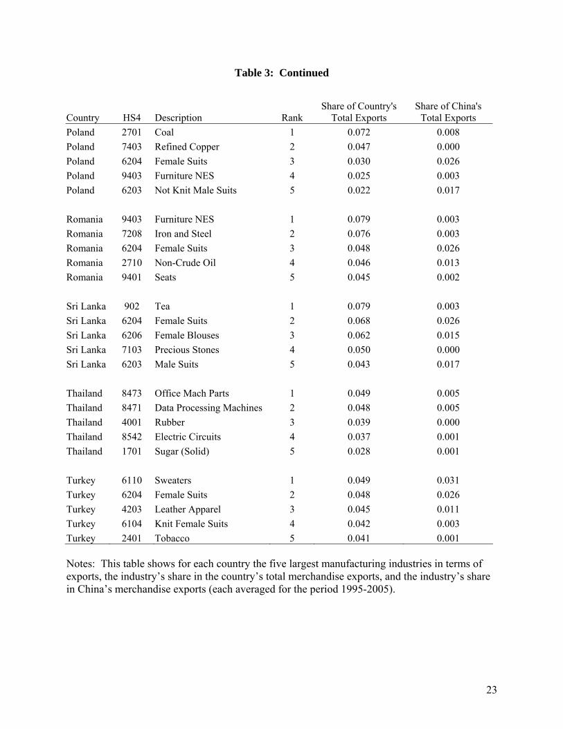
To provide some background on the industries included in the sample, Table 3 shows the
5 largest industries in terms of manufacturing exports for each of the 10 developing-country
exporters. For 9 of the countries (all except Hungary), manufacturing exports are concentrated in
a handful of industries, with the top 5 industries accounting for at least 20% of merchandise
exports, and for 5 of the countries, the top 5 industries account for at least 30% of merchandise
exports. For 7 of the countries, at least one of their top 5 export industries is also one that
accounts for at least 2% of China’s manufacturing exports.
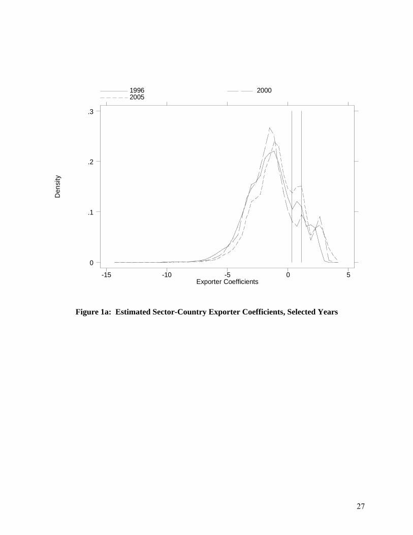
The regression results for equation (4) involve a large amount of output. In each year, we
estimate over 10,000 country-sector exporter coefficients and country-sector importer
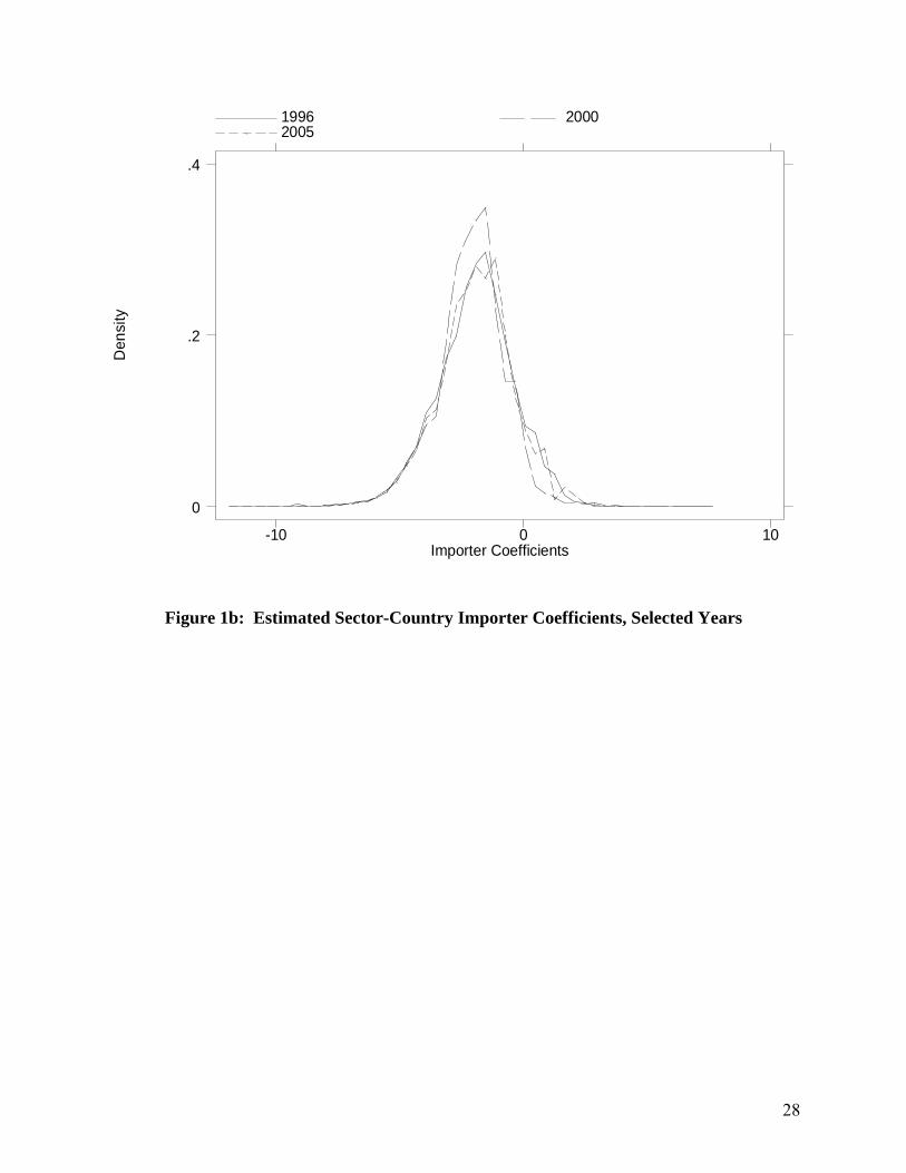
coefficients and over 200 trade-cost coefficients. To summarize exporter and import dummies
compactly, Figures 1a and 1b plot kernel densities for the sector-country exporter and importer
coefficients (where the densities are weighted by sector-country exports or imports). Figure 1a
shows that most exporter coefficients are negative, consistent with sectoral exports for most
countries being below the United States. Over the sample period, the distribution of exporter
coefficients shifts to the right, suggesting other countries are catching up to the United States.
8 This restriction may introduce selection bias into the estimation.
12
Vertical lines indicate weighted mean values for China’s exporter coefficients in 1995 (equal to
0.44) and 2005 (equal to 1.78), which rise in value over time relative to the overall distribution of
exporter coefficients, suggesting China’s export-supply capacity has improved relative to other
countries over the sample period. Evidence we report later supports this finding. In Figure 1b,
most importer coefficients are also negative, again indicating sectoral trade values for most
countries are below those for the United States.
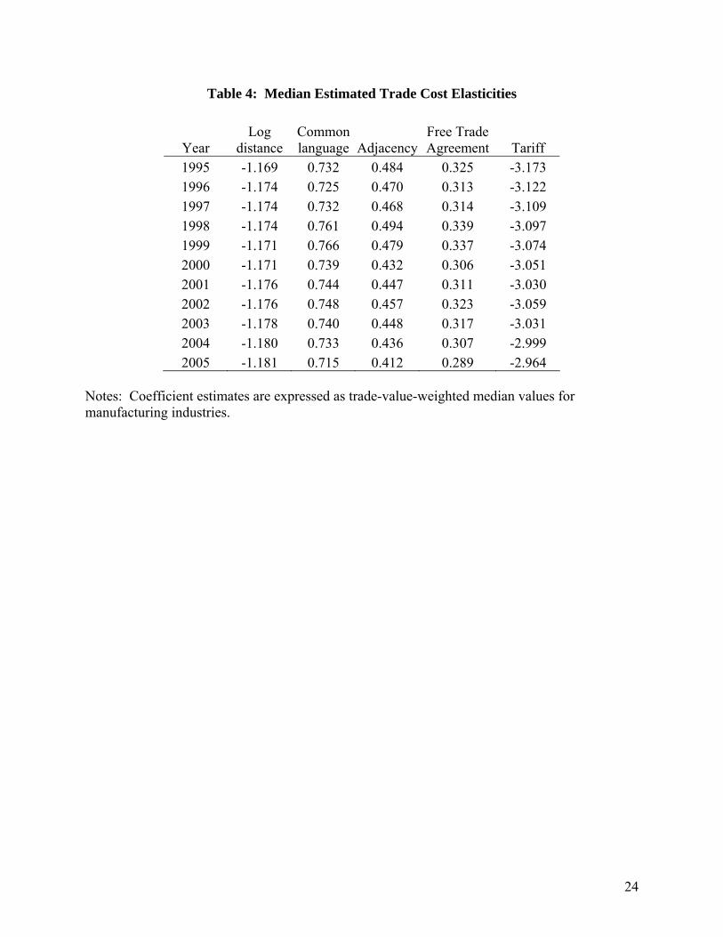
To provide further detail on the coefficient estimates, Table 4 gives median values of the
trade cost elasticities by year, weighted by each sector’s share of world trade. The estimates are
in line with results in the literature (Anderson and van Wincoop, 2004). The coefficient on log
distance is negative and slightly larger than one in absolute value; adjacency, common language,
and joint membership in a free trade agreement are each associated with higher levels of bilateral
trade; and the implied elasticity of substitution (given by the tariff coefficient) is close to 3.
3.2 Export Supply Capabilities in Developing Countries vis-à-vis China
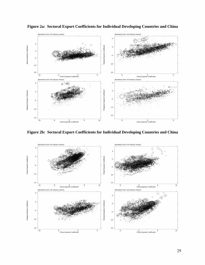
Of primary interest is how the 10 countries’ export-supply capacities compare to those of
China. Figures 2a-2c plot sectoral export coefficients for each country against exporter
coefficients for China over the sample period (using sectoral shares of annual manufacturing
exports in each country as weights). For each country, there is a positive correlation in its
sectoral export dummies with China, with the correlation being strongest for Turkey (0.63),
Romania (0.59), Hungary (0.48), Thailand (0.48), Malaysia (0.47), Poland (0.45), Sri Lanka
(0.45); somewhat smaller for the Philippines (0.33) and Pakistan (0.32); and weakest for Mexico
(0.12). The correlation for Mexico appears to be driven by industries related to petroleum, which
began the period as major export sectors for the country but have since declined in importance.
13
The positive correlation in sectoral export coefficients with China suggests that most of
the large developing countries that specialize in manufacturing have strong export supply
capabilities in the same sectors in which China is also strong. In other words, the comparative
advantage of these countries is closely aligned with that of China. To the extent that the major
trading partners of these countries are the same as those of China, they would be exposed to
export-supply shocks in China, meaning that growth in China would potentially reduce demand
for the manufacturing exports that they produce and lower their terms of trade.
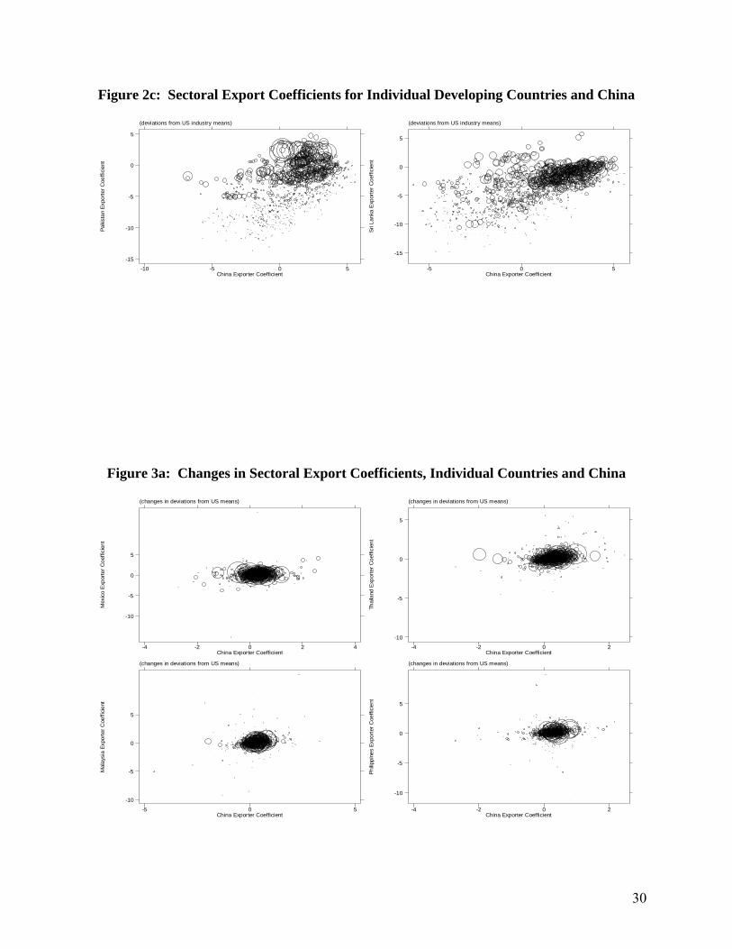
To see how export supply capacities have evolved over time, Figures 3a-3c plot the year-
on-year change in country-sector export dummies for each of the 10 developing countries against
those for China, weighted by each country’s sectoral trade shares. Immediately apparent is that
the range of growth in China’s export-supply capacities is large relative to that of any other
developing country. Changes in China’s export dummies take on a wide range of values, while
none of the 10 countries shows nearly as much variation. As a consequence, the correlation
between changes in sectoral export dummies between each country and China is weaker than the
correlation in levels. The strongest correlations in changes are for Romania (0.50) and Malaysia
(0.47); followed by Thailand (0.32), Sri Lanka (0.31), Hungary (0.30), the Philippines (0.30),
Poland (0.22), and Turkey (0.21); and then by Pakistan (0.16) and Mexico (0.14).
4. Counterfactual Exercises
In this section, we compare the change in import demand conditions facing each of the 10
developing-country exporters under two scenarios, one in which import demand evolved as
observed in the data (as implied by the coefficient estimates from the gravity model) and a
second in which we hold constant the change in China’s export-supply capabilities. This
14
exercise allows us to examine whether China’s growth in export production has represented a
negative shock to the demand for exports from other developing countries.
According to the theory presented in section 2, sectoral import demand in a country is
affected by its GDP and by its sectoral import price index. Its price index, in turn, is affected by
export supply conditions in the countries from which it imports goods, weighted by trade costs with
these countries. From equation (8), this yields the following relationship:
1n 2nnhtH ˆ ˆs
nkt 0 1 kt 2 nktnhkt hkh 1
m ln Y ln e dβ β
=
⎛ ⎞= α +α +α τ + η⎜ ⎟⎜ ⎟
⎝ ⎠∑ , (10)
where nht nht 1n 2nˆ ˆˆ ˆm , s , , andβ β are OLS coefficient estimates of the sectoral importer dummy, the
sectoral exporter dummy, the tariff elasticity, and the distance elasticity from equation (4). In
theory, it should be the case that α1=1 and α2=-1.
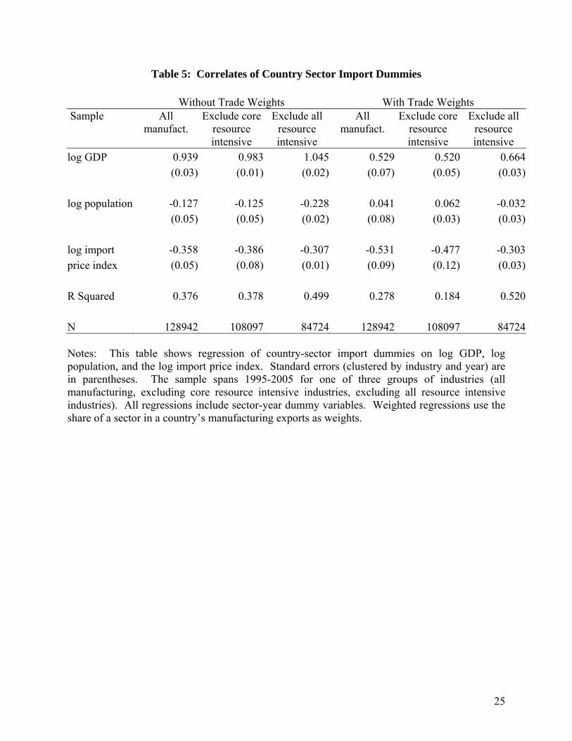
To verify that the relationships posited by theory are found in the data, Table 5 shows
coefficient estimates for equation (10). Departing from equation (10) slightly, we also include
log population as an explanatory variable (to allow demand to be affected by market size and
average income), though it is imprecisely estimated in most regressions. We show specifications
under alternative weighting schemes and for three sets of industries: all manufacturing industries,
excluding core resource-intensive industries,9 and excluding all resource-intensive industries.10
Demand conditions in resource-intensive industries may differ from other manufacturing
industries due to their reliance on primary commodities as inputs. Coefficients on GDP (α1 in
equation (10)) are all positive and precisely estimated, ranging in value from 0.52 to 1.05.
Coefficients on the import price index (α2 in (10)) are all negative and precisely estimated,
9 At the two-digit HS level, these industries are beverages, cereals, animal oils and fats, sugar, meat and seafood processing, fruit and vegetable processing, tobacco, non-metallic minerals, mineral fuels and oils, and inorganic chemicals. 10 In addition to those industries mentioned in note 9, this excludes organic chemicals, pharmaceuticals, fertilizers, plastics, rubber, leather products, and wood products.
15
ranging in value from -0.31 to -0.53. While the coefficient estimates do not exactly match the
theoretically predictions, they are broadly consistent with the model.
The next exercise is to use the coefficient estimates to examine the difference in demand
for exports faced by the 10 developing country exporters that is associated with the growth in
China’s export supply capacity. The first step is to calculate for each importer in each sector the
value in equation (9), which is,
1n 2n 1n 2n 1n 2n 1n 2nnht nc0 nht nctH Hˆ ˆ ˆ ˆ ˆ ˆ ˆ ˆˆ ˆ ˆ ˆs s s s
nkt nkt nhkt hk nckt ck nhkt hk nckt ckh c h c
m m ln e d e d ln e d e dβ β β β β β β β
≠ ≠
⎡ ⎤⎛ ⎞ ⎛ ⎞− = − τ + τ − τ + τ⎢ ⎥⎜ ⎟ ⎜ ⎟⎜ ⎟ ⎜ ⎟⎢ ⎥⎝ ⎠ ⎝ ⎠⎣ ⎦
∑ ∑ .
This shows the amount by which average import demand in country k and sector n at time t
would have differed had China’s export supply capacity (which reflects the number of product
varieties it produces and its production costs) had remained constant between time 0 and time t.11
The second step is to calculate the weighted average value of nkt nktm m− for each of the 10
developing country exporters, using as weights the share of each importer and sector in a country’s
total manufacturing exports (where these shares are averages over the sample period).12
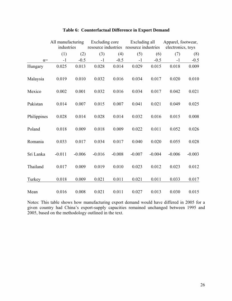
Table 6 shows the results from the counterfactual calculation where year 0 corresponds to
1995 and year t corresponds to 2005.13 The first column shows results in which we set α2 from
equation (10) equal to -1, as implied by theory. In 2005, the difference in export demand ranges
11 An alternative to the counterfactual exercise we propose would be to examine the change in China’s exports implied by the change in tariffs facing China over the sample period. Were China’s economy in steady state, then the change in tariffs would be the primary shock affecting the country’s exports. However, over the sample period China very much appears to be an economy in transition to a new steady state, associated with a sectoral and regional reallocation of resources brought about by the end of central planning. Thus, focusing on tariffs alone would miss the primary shock to China’s export growth. 12 In taking this weighted average across industries, we are approximating for the percentage change in imports with the log change. This approximation becomes less precise as the growth in imports becomes larger. In unreported results, we experimented with using the percentage change. The findings are similar to what we report in Table 6. 13 Because we do not estimate equation (4) subject to the constraint in equation (6), one needs to be careful in interpreting our results. The counterfactual exercises we report apply to changes in demand conditions rather than changes in trade. Absent imposing the equilibrium conditions implied by the model, we cannot interpret the counterfactual exercises as implying how trade would change.
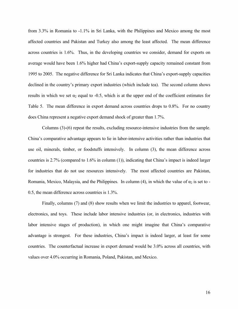
16
from 3.3% in Romania to -1.1% in Sri Lanka, with the Philippines and Mexico among the most
affected countries and Pakistan and Turkey also among the least affected. The mean difference
across countries is 1.6%. Thus, in the developing countries we consider, demand for exports on
average would have been 1.6% higher had China’s export-supply capacity remained constant from
1995 to 2005. The negative difference for Sri Lanka indicates that China’s export-supply capacities
declined in the country’s primary export industries (which include tea). The second column shows
results in which we set α2 equal to -0.5, which is at the upper end of the coefficient estimates for
Table 5. The mean difference in export demand across countries drops to 0.8%. For no country
does China represent a negative export demand shock of greater than 1.7%.
Columns (3)-(6) repeat the results, excluding resource-intensive industries from the sample.
China’s comparative advantage appears to lie in labor-intensive activities rather than industries that
use oil, minerals, timber, or foodstuffs intensively. In column (3), the mean difference across
countries is 2.7% (compared to 1.6% in column (1)), indicating that China’s impact is indeed larger
for industries that do not use resources intensively. The most affected countries are Pakistan,
Romania, Mexico, Malaysia, and the Philippines. In column (4), in which the value of α2 is set to -
0.5, the mean difference across countries is 1.3%.
Finally, columns (7) and (8) show results when we limit the industries to apparel, footwear,
electronics, and toys. These include labor intensive industries (or, in electronics, industries with
labor intensive stages of production), in which one might imagine that China’s comparative
advantage is strongest. For these industries, China’s impact is indeed larger, at least for some
countries. The counterfactual increase in export demand would be 3.0% across all countries, with
values over 4.0% occurring in Romania, Poland, Pakistan, and Mexico.
17
The counterfactual exercises indicate that had China’s export-supply capacities remained
unchanged demand for exports would have been modestly larger for other developing countries that
specialize in manufacturing exports. To repeat, across all manufacturing industries, the average
difference in export demand is 0.8% to 1.6%; for non-resource-intensive industries, the average
difference is 1.3% to 2.7%. These are hardly large values, suggesting that even for the countries
that would appear to be most adversely affected by China’s growth it is difficult to find evidence
that the demand for their exports has been significantly reduced by China’s expansion.
5. Discussion
In this paper, we use the gravity model of trade to examine the impact of China’s growth
on the demand for exports in developing countries that specialize in manufacturing. China’s
high degree of specialization in manufacturing makes its expansion a potentially significant
shock for other countries that are also manufacturing oriented. Of the 10 developing countries
we examine, 9 have a pattern of comparative advantage that strongly overlaps with China, as
indicated by countries’ estimated export-supply capacities. Yet, despite the observed similarities
in export patterns, we find that China’s growth represents only a small negative shock in demand
for the other developing countries’ exports. While there is anxiety in many national capitals over
China’s continued export surge, our results suggest China’s impact on the export market share of
other manufacturing exporters has been relatively small.
There are several important caveats to our results. Our framework and analysis are
confined to manufacturing industries. There may be important consequences of China for
developing-country commodity trade, which we do not capture. The counterfactual exercises we
report do not account for general-equilibrium effects. There could be feedback effects from

18
China’s growth on prices, wages, and the number of product varieties produced that cause us to
misstate the consequences of such shocks for other developing countries. There are also
concerns about the consistency of the coefficient estimates, due to the fact that we do not account
for why there is zero trade between some countries.
19
References
Anderson, James E. and Van Wincoop, Eric. “Trade Costs.” Journal of Economic Literature, September 2004.
Broda, Christian, and David Weinstein. 2006. “Globalization and the Gains from Variety.” Quarterly Journal of Economics, 121(2).
Devlin, Robert, Antoni Estevadeordal, and Andrés Rodriguez-Clare. 2005. The Emergence of China: Opportunities and Challenges for Latin America and the Caribbean. Washington, DC: Inter-American Development Bank.
Eichengreen, Barry, and Hui Tong. 2005. “Is China’s FDI Coming at the Expense of Other Countries?” NBER Working Paper No. 11335.
Feenstra, Robert C. Advanced International Trade: Theory and Evidence. Princeton: Princeton University Press, 2003.
Feenstra, Robert C., Robert Lipsey, Haiyan Deng, Alyson C. Ma, and Hengyong Mo. 2005. “World Trade Flows: 1962-2000.” NBER Working Paper No. 11040.
Helpman, Elhanan, Marc J. Melitz, and Yona Rubinstein. 2007. “Trading Partners and Trading Volumes,” mimeo, Harvard University.
Lopez Cordoba, Ernesto, Alejandro Micco, and Danielken Molina. 2005. “How Sensitive Are Latin American Exports to Chinese Competition in the U.S. Market?” Mimeo, Inter-American Development Bank.
Robertson, Raymond (2007) “World Trade and Tariff Data” mimeo, Macalester College Santos Silva, J.M.C., and Silvana Tenreryo. 2005. “The Log of Gravity.” The Review of
Economics and Statistics, forthcoming. Wooldridge, Jeffrey M. 2002. Econometric Analysis of Cross Section and Panel Data.
Cambridge, MA: MIT Press.
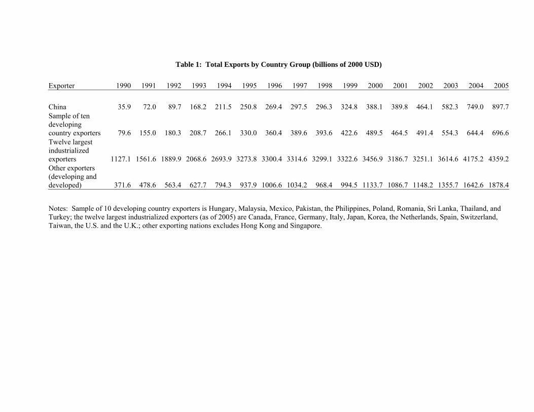
Table 1: Total Exports by Country Group (billions of 2000 USD)
Exporter 1990 1991 1992 1993 1994 1995 1996 1997 1998 1999 2000 2001 2002 2003 2004 2005 China 35.9 72.0 89.7 168.2 211.5 250.8 269.4 297.5 296.3 324.8 388.1 389.8 464.1 582.3 749.0 897.7 Sample of ten developing country exporters 79.6 155.0 180.3 208.7 266.1 330.0 360.4 389.6 393.6 422.6 489.5 464.5 491.4 554.3 644.4 696.6 Twelve largest industrialized exporters 1127.1 1561.6 1889.9 2068.6 2693.9 3273.8 3300.4 3314.6 3299.1 3322.6 3456.9 3186.7 3251.1 3614.6 4175.2 4359.2 Other exporters (developing and developed) 371.6 478.6 563.4 627.7 794.3 937.9 1006.6 1034.2 968.4 994.5 1133.7 1086.7 1148.2 1355.7 1642.6 1878.4
Notes: Sample of 10 developing country exporters is Hungary, Malaysia, Mexico, Pakistan, the Philippines, Poland, Romania, Sri Lanka, Thailand, and Turkey; the twelve largest industrialized exporters (as of 2005) are Canada, France, Germany, Italy, Japan, Korea, the Netherlands, Spain, Switzerland, Taiwan, the U.S. and the U.K.; other exporting nations excludes Hong Kong and Singapore.
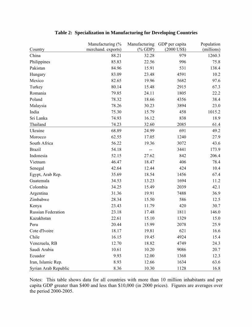
Table 2: Specialization in Manufacturing for Developing Countries
Country Manufacturing (%
merchand. exports)Manufacturing
(% GDP)GDP per capita
(2000 US$) Population (millions)
China 88.21 32.28 979 1260.3Philippines 85.83 22.56 996 75.8Pakistan 84.96 15.91 531 138.4Hungary 83.09 23.48 4591 10.2Mexico 82.65 19.96 5682 97.6Turkey 80.14 15.48 2915 67.3Romania 79.85 24.11 1805 22.2Poland 78.32 18.66 4356 38.4Malaysia 78.26 30.23 3894 23.0India 75.30 15.79 458 1015.2Sri Lanka 74.93 16.12 838 18.9Thailand 74.23 32.60 2085 61.4Ukraine 68.89 24.99 691 49.2Morocco 62.55 17.05 1240 27.9South Africa 56.22 19.36 3072 43.6Brazil 54.18 -- 3441 173.9Indonesia 52.15 27.62 842 206.4Vietnam 46.47 18.47 406 78.4Senegal 42.64 12.44 424 10.4Egypt, Arab Rep. 35.69 18.54 1456 67.4Guatemala 34.53 13.23 1694 11.2Colombia 34.25 15.49 2039 42.1Argentina 31.36 19.91 7488 36.9Zimbabwe 28.34 15.50 586 12.5Kenya 23.43 11.79 420 30.7Russian Federation 23.18 17.48 1811 146.0Kazakhstan 22.61 15.10 1329 15.0Peru 20.44 15.99 2078 25.9Cote d'Ivoire 18.17 19.81 621 16.6Chile 16.15 19.45 4924 15.4Venezuela, RB 12.70 18.82 4749 24.3Saudi Arabia 10.61 10.20 9086 20.7Ecuador 9.93 12.00 1368 12.3Iran, Islamic Rep. 8.93 12.66 1634 63.6Syrian Arab Republic 8.36 10.30 1128 16.8 Notes: This table shows data for all countries with more than 10 million inhabitants and per capita GDP greater than $400 and less than $10,000 (in 2000 prices). Figures are averages over the period 2000-2005.
22
Table 3: Major Export Industries in 10 Developing Countries
Country HS4 Description Mfg rankShare of Country's
Total Exports Share of China's
Total Exports Hungary 6204 Female Suits 1 0.035 0.026 Hungary 6403 Footwear 2 0.026 0.024 Hungary 8544 Wire 3 0.023 0.003 Hungary 2710 Non-Crude Oil 4 0.022 0.013 Hungary 8708 Motor Vehicle Parts 5 0.020 0.001 Malaysia 2709 Crude Oil 1 0.103 0.048 Malaysia 8542 Electric Circuits 2 0.087 0.001 Malaysia 4403 Rough Wood 3 0.060 0.001 Malaysia 8527 Receivers 4 0.050 0.023 Malaysia 4407 Sawn Wood 5 0.038 0.001 Mexico 2709 Crude Oil 1 0.219 0.048 Mexico 8703 Motor Vehicles 2 0.066 0.000 Mexico 8708 Motor Vehicle Parts 3 0.054 0.001 Mexico 8544 Wire 4 0.041 0.003 Mexico 8407 Engines 5 0.036 0.000 Pakistan 5205 Cotton Yarn 1 0.186 0.002 Pakistan 5201 Cotton 2 0.097 0.004 Pakistan 5208 Cotton Fabrics 3 0.063 0.010 Pakistan 6302 House Linens 4 0.061 0.010 Pakistan 4203 Leather Apparel 5 0.056 0.011 Philippines 8542 Electric Circuits 1 0.124 0.001 Philippines 1513 Coconut Oil 2 0.037 0.000 Philippines 8471 Data Processing Machines 3 0.031 0.005 Philippines 2603 Copper 4 0.029 0.000 Philippines 7403 Refined Copper 5 0.027 0.000
23
Table 3: Continued
Country HS4 Description Rank Share of Country's
Total Exports Share of China's
Total Exports Poland 2701 Coal 1 0.072 0.008 Poland 7403 Refined Copper 2 0.047 0.000 Poland 6204 Female Suits 3 0.030 0.026 Poland 9403 Furniture NES 4 0.025 0.003 Poland 6203 Not Knit Male Suits 5 0.022 0.017 Romania 9403 Furniture NES 1 0.079 0.003 Romania 7208 Iron and Steel 2 0.076 0.003 Romania 6204 Female Suits 3 0.048 0.026 Romania 2710 Non-Crude Oil 4 0.046 0.013 Romania 9401 Seats 5 0.045 0.002 Sri Lanka 902 Tea 1 0.079 0.003 Sri Lanka 6204 Female Suits 2 0.068 0.026 Sri Lanka 6206 Female Blouses 3 0.062 0.015 Sri Lanka 7103 Precious Stones 4 0.050 0.000 Sri Lanka 6203 Male Suits 5 0.043 0.017 Thailand 8473 Office Mach Parts 1 0.049 0.005 Thailand 8471 Data Processing Machines 2 0.048 0.005 Thailand 4001 Rubber 3 0.039 0.000 Thailand 8542 Electric Circuits 4 0.037 0.001 Thailand 1701 Sugar (Solid) 5 0.028 0.001 Turkey 6110 Sweaters 1 0.049 0.031 Turkey 6204 Female Suits 2 0.048 0.026 Turkey 4203 Leather Apparel 3 0.045 0.011 Turkey 6104 Knit Female Suits 4 0.042 0.003 Turkey 2401 Tobacco 5 0.041 0.001 Notes: This table shows for each country the five largest manufacturing industries in terms of exports, the industry’s share in the country’s total merchandise exports, and the industry’s share in China’s merchandise exports (each averaged for the period 1995-2005).
24
Table 4: Median Estimated Trade Cost Elasticities
Year Log
distance Common language Adjacency
Free Trade Agreement Tariff
1995 -1.169 0.732 0.484 0.325 -3.173 1996 -1.174 0.725 0.470 0.313 -3.122 1997 -1.174 0.732 0.468 0.314 -3.109 1998 -1.174 0.761 0.494 0.339 -3.097 1999 -1.171 0.766 0.479 0.337 -3.074 2000 -1.171 0.739 0.432 0.306 -3.051 2001 -1.176 0.744 0.447 0.311 -3.030 2002 -1.176 0.748 0.457 0.323 -3.059 2003 -1.178 0.740 0.448 0.317 -3.031 2004 -1.180 0.733 0.436 0.307 -2.999 2005 -1.181 0.715 0.412 0.289 -2.964
Notes: Coefficient estimates are expressed as trade-value-weighted median values for manufacturing industries.
25
Table 5: Correlates of Country Sector Import Dummies Without Trade Weights With Trade Weights Sample All
manufact.
Exclude core resource intensive
Exclude all resource intensive
All manufact.
Exclude core resource intensive
Exclude all resource intensive
log GDP 0.939 0.983 1.045 0.529 0.520 0.664 (0.03) (0.01) (0.02) (0.07) (0.05) (0.03) log population -0.127 -0.125 -0.228 0.041 0.062 -0.032 (0.05) (0.05) (0.02) (0.08) (0.03) (0.03) log import -0.358 -0.386 -0.307 -0.531 -0.477 -0.303price index (0.05) (0.08) (0.01) (0.09) (0.12) (0.03) R Squared 0.376 0.378 0.499 0.278 0.184 0.520 N 128942 108097 84724 128942 108097 84724 Notes: This table shows regression of country-sector import dummies on log GDP, log population, and the log import price index. Standard errors (clustered by industry and year) are in parentheses. The sample spans 1995-2005 for one of three groups of industries (all manufacturing, excluding core resource intensive industries, excluding all resource intensive industries). All regressions include sector-year dummy variables. Weighted regressions use the share of a sector in a country’s manufacturing exports as weights.
26
Table 6: Counterfactual Difference in Export Demand
All manufacturing
industries Excluding core
resource industriesExcluding all
resource industriesApparel, footwear,
electronics, toys (1) (2) (3) (4) (5) (6) (7) (8)
α= -1 -0.5 -1 -0.5 -1 -0.5 -1 -0.5Hungary 0.025 0.013 0.028 0.014 0.029 0.015 0.018 0.009 Malaysia 0.019 0.010 0.032 0.016 0.034 0.017 0.020 0.010 Mexico 0.002 0.001 0.032 0.016 0.034 0.017 0.042 0.021 Pakistan 0.014 0.007 0.015 0.007 0.041 0.021 0.049 0.025 Philippines 0.028 0.014 0.028 0.014 0.032 0.016 0.015 0.008 Poland 0.018 0.009 0.018 0.009 0.022 0.011 0.052 0.026 Romania 0.033 0.017 0.034 0.017 0.040 0.020 0.055 0.028 Sri Lanka -0.011 -0.006 -0.016 -0.008 -0.007 -0.004 -0.006 -0.003 Thailand 0.017 0.009 0.019 0.010 0.023 0.012 0.023 0.012 Turkey 0.018 0.009 0.021 0.011 0.021 0.011 0.033 0.017 Mean 0.016 0.008 0.021 0.011 0.027 0.013 0.030 0.015 Notes: This table shows how manufacturing export demand would have differed in 2005 for a given country had China’s export-supply capacities remained unchanged between 1995 and 2005, based on the methodology outlined in the text.
27
Den
sity
Exporter Coefficients
1996 2000 2005
-15 -10 -5 0 5
0
.1
.2
.3
Figure 1a: Estimated Sector-Country Exporter Coefficients, Selected Years
28
Den
sity
Importer Coefficients
1996 2000 2005
-10 0 10
0
.2
.4
Figure 1b: Estimated Sector-Country Importer Coefficients, Selected Years
29
Figure 2a: Sectoral Export Coefficients for Individual Developing Countries and China
(deviations from US industry means)
Mex
ico
Exp
orte
r Coe
ffici
ent
China Exporter Coefficient-10 -5 0 5
-15
-10
-5
0
5
(deviations from US industry means)
Thai
land
Exp
orte
r Coe
ffici
ent
China Exporter Coefficient-5 0 5
-15
-10
-5
0
5
(deviations from US industry means)
Mal
aysi
a Ex
porte
r Coe
ffici
ent
China Exporter Coefficient-10 -5 0 5 10
-15
-10
-5
0
5
(deviations from US industry means)
Philip
pine
s Ex
porte
r Coe
ffici
ent
China Exporter Coefficient-5 0 5
-15
-10
-5
0
5
Figure 2b: Sectoral Export Coefficients for Individual Developing Countries and China
(deviations from US industry means)
Turk
ey E
xpor
ter C
oeffi
cien
t
China Exporter Coefficient-10 -5 0 5 10
-15
-10
-5
0
5
(deviations from US industry means)
Pola
nd E
xpor
ter C
oeffi
cien
t
China Exporter Coefficient-5 0 5 10
-15
-10
-5
0
5
(deviations from US industry means)
Hun
gary
Exp
orte
r Coe
ffici
ent
China Exporter Coefficient-10 -5 0 5
-15
-10
-5
0
5
(deviations from US industry means)
Rom
ania
Exp
orte
r Coe
ffici
ent
China Exporter Coefficient-5 0 5 10
-15
-10
-5
0
5
30
Figure 2c: Sectoral Export Coefficients for Individual Developing Countries and China
(deviations from US industry means)
Paki
stan
Exp
orte
r Coe
ffici
ent
China Exporter Coefficient-10 -5 0 5
-15
-10
-5
0
5
(deviations from US industry means)
Sri L
anka
Exp
orte
r Coe
ffici
ent
China Exporter Coefficient-5 0 5
-15
-10
-5
0
5
Figure 3a: Changes in Sectoral Export Coefficients, Individual Countries and China
(changes in deviations from US means)
Mex
ico
Exp
orte
r Coe
ffici
ent
China Exporter Coefficient-4 -2 0 2 4
-10
-5
0
5
(changes in deviations from US means)
Thai
land
Exp
orte
r Coe
ffici
ent
China Exporter Coefficient-4 -2 0 2
-10
-5
0
5
(changes in deviations from US means)
Mal
aysi
a Ex
porte
r Coe
ffici
ent
China Exporter Coefficient-5 0 5
-10
-5
0
5
(changes in deviations from US means)
Philip
pine
s Ex
porte
r Coe
ffici
ent
China Exporter Coefficient-4 -2 0 2
-10
-5
0
5

31
Figure 3b: Changes in Sectoral Export Coefficients, Individual Countries and China
(changes in deviations from US means)
Turk
ey E
xpor
ter C
oeffi
cien
t
China Exporter Coefficient-5 0 5
-10
-5
0
5
(changes in deviations from US means)
Pola
nd E
xpor
ter C
oeffi
cien
t
China Exporter Coefficient-5 0 5
-10
-5
0
5
(changes in deviations from US means)
Hun
gary
Exp
orte
r Coe
ffici
ent
China Exporter Coefficient-2 0 2 4
-10
-5
0
5
(changes in deviations from US means)
Rom
ania
Exp
orte
r Coe
ffici
ent
China Exporter Coefficient-5 0 5
-10
-5
0
5
Figure 3c: Changes in Sectoral Export Coefficients, Individual Countries and China
(changes in deviations from US means)
Paki
stan
Exp
orte
r Coe
ffici
ent
China Exporter Coefficient-2 -1 0 1 2
-10
-5
0
5
(changes in deviations from US means)
Sri L
anka
Exp
orte
r Coe
ffici
ent
China Exporter Coefficient-4 -2 0 2
-10
-5
0
5