china’s growth success including the degree of openness, · pdf filechina’s growth...
TRANSCRIPT

1
Why has China Grown so Fast? The Role of Structural Change
Sai Ding and John Knight
Department of Economics University of Oxford Manor Road Building
Oxford OX1 3UQ [email protected]
Abstract In this paper we attempt to explore some indirect determinants of
China’s growth success including the degree of openness, institutional change and
sectoral change, based on a cross-province dataset. The methodology we adopt is the
informal growth regression, which permits the introduction of some explanatory
variables that represent the underlying as well as the proximate causes of growth.
We first address the problem of model uncertainty by adopting two approaches to
model selection, BMA and GETS, to consider a wide range of candidate predictors of
growth in China. Then variables flagged as being important by these procedures are
used in formulating our models, in which the contribution of factors behind the
proximate determinants are examined in some detail using panel data system GMM.
All three forms of structural change -- relative expansion of the trade sector, of the
private sector, and of the non-agricultural sector -- are found to raise the growth rate.
Moreover, structural change in all three dimensions was rapid over the study period.
Each change primarily represents an improvement in the efficiency of the economy,
moving it towards its production frontier. We conclude that such improvements in
productive efficiency have been an important part of the explanation for China's
remarkable rate of growth.
Keywords Economic growth; Structural change; Openness; Institutional change;
China
JEL Classification O40; O53
Acknowledgement We are grateful to Adrian Wood for constructive comments and
to Antoni Chawluk, Linda Yueh and other participants in the Economies of
Transition Seminar at St Antony College, Oxford for insightful discussion. The
financial support of the Leverhulme Trust is gratefully acknowledged.

2
1. Introduction
Since economic reform commenced in 1978, the Chinese economy has experienced
remarkable economic growth. The growth rate of GDP per capita has averaged 8.6 percent
per annum over the thirty-year period 1978-2007. Nor is there any sign of deceleration in
growth: over the years 2000-07, the equivalent figure was 9.2 percent, and China accounted
for about 35 percent of the growth in world GDP at PPP prices1. For a major country – China
accounts for more than one-fifth of world population – such rapid progress is unprecedented.
It is all the more remarkable in the light of China’s poverty – over 300 million people have
been lifted out of one-dollar-a-day poverty since 19782 – and of its difficult transition from
being a centrally planned, closed economy at the start of reform towards becoming a market
economy.
In this paper we explore the reasons for China’s growth success using a cross-province
dataset spanning three decades. Our purpose is to explain why China as a whole, and indeed
all its provinces, has grown so fast. Our expectation is that the analysis of provincial time
series data will reveal more information about the various determinants of economic growth
than would an aggregate time series analysis. The use of provincial data expands the sample
size substantially.
Economists are better able to analyse the direct than the indirect determinants of
growth, and yet these conventional variables may simply represent associations that are
themselves to be explained by causal processes. There are three possible empirical
approaches: growth accounting, structural growth modelling, and informal growth regression.
In contrast to the former two, the third approach permits the introduction of some explanatory
variables that represent the underlying as well as the proximate causes of growth. Unlike the
growth accounting method, it does not involve the task of measuring the capital stock and
thus it avoids making several assumptions about unknown parameters such as factor shares of
income and the depreciation rate of capital. Two further arguments make us less inclined to
use the growth accounting approach. Firstly, when total factor productivity (TFP) growth is
measured as a residual, i.e. as the growth rate in GDP that cannot be accounted for by the
growth of the observable inputs, it should not be equated with technological change as many
1 Based on new statistical calculations of PPP exchange rates published in December 2007 by the International
Comparison Program (ICP), the World Bank and IMF recently revised downward their estimates for China's
PPP-based GDP by around 40 percent. Despite this revision, China remains the main driver of global growth.
For example, it contributed nearly 27 percent of world GDP growth in 2007 using the new PPP figure. 2 The figure is calculated from Ravallion and Chen (2007).

3
researchers have done. Rather it is 'a measure of ignorance' (Abramovitz, 1986), covering
many factors like structural change, improvement in allocative efficiency, economies of
scale, and other omitted variables and measurement errors. Secondly, although growth
accounting provides a convenient way to allow for the breakdown of observed growth of
GDP into components associated with changes in factor inputs and in production
technologies, we are not convinced that technological change and investment are separable in
reality, i.e. changing technology requires investment, and investment inevitably involves
technological change. This is consistent with the view of Scott (1989) that technological
change and investment are part and parcel of the same thing and that separation is
meaningless. Hence, informal growth regression is the methodology that we adopt.
A feature of our study is to use recently developed approaches to model selection in
order to construct empirical models based on robust predictors. It is widely believed that
growth theories are not explicit enough about variables that should be included in the
empirical growth models. The issue of model uncertainty has attracted much research
attention in the context of cross-country growth regressions. However, to the best of our
knowledge, it has been largely ignored in cross-province growth studies of China, i.e. the
existing literature has not explicitly or systematically considered the issue of model selection
before any investigation of particular causes of China's growth. We first use two leading
model selection approaches, Bayesian Model Averaging and the automated General-to-
Specific approach, to examine the association between the growth rate of real GDP per capita
and a large range of potential explanatory variables. These include the initial level of income,
fixed capital formation, human capital formation, population growth, the degree of openness,
institutional change, sectoral change, financial development, infrastructure and regional
advantage. The variables flagged as being important by these procedures are then used in
formulating our baseline model, which is estimated using panel data system GMM to control
for problems of omitted variables, endogeneity and measurement error of regressors. In the
second stage, we also examine the robustness of our selected model and the contribution of
the main variables. In a companion paper (Ding and Knight, 2008b), our focus is on the
growth impact of various types of physical and human capital investment. In this paper, our
focus is on variables that do not enter formal growth models.
In Section 2 we provide the background to Chinese economic growth, as an aid to
interpretation. Section 3 is a literature survey which offers guidance on the choice of
variables in our general model. Section 4 explains the empirical methodology and describes

4
the dataset. Section 5 reports the results of our basic equations and their interpretation. The
contribution of three dimensions of structural change -- degree of openness, institutional
change, and sectoral change -- is then examined in detail in sections 6-8. Section 9
summarises and concludes.
2. Background to China’s growth
The growth of the Chinese economy since the start of its economic reform has been a
process of ‘crossing the river by groping for the stepping stones’, as described by Deng
Xiaoping: no stereotype reform package was adopted in advance. One reform begat the need,
or the opportunity, for another, and the process became cumulative. The reforms were
incremental but hardly slow: huge changes have occurred in less than three decades, as China
has moved from central planning towards a market economy. It is relevant that China’s had
been a labour surplus economy par excellence: labour was underemployed in the farms and in
the urban state enterprises: government preferred unemployment to be disguised and shared
rather than open and threatening (Knight and Song, 2005, chs. 2, 6, and 8). New sectors could
thus be expanded without loss of output elsewhere.
The first stage of economic reform (1978-84) concentrated on the rural areas. The
communes were disbanded and individual incentives were restored. Farming households
(then 82 percent of the population) were given use-rights to collectively-owned land under
long term leases, and the right to sell their marginal produce on the open market. Rural non-
farm enterprises were permitted, and they stepped in to produce the light manufactures that
the urban state-owned enterprises (SOEs) generally failed to supply. Rural credit constraints
encouraged household saving. Rural production rose rapidly as farms became more efficient,
as surplus labour was used more productively in rural industry, and as rural entrepreneurship,
saving and investment responded to the new opportunities.
The second stage of economic reform (1985-92) was an incremental process of
reforming the urban economy, in particular the SOEs, which were gradually given greater
managerial autonomy. The principal-agent problem inherent in state ownership limited the
efficiency of SOEs but competition from other market participants – initially village and
township enterprises and later domestic and foreign privately owned enterprises as well as
from imports – grew steadily.
The third stage of economic reform (1993- ) was ignited by Deng Xiaoping’s ‘Southern
Tour’ to mobilise support for more radical reforms. The private sector – for the first time
5
acknowledged and accepted – was invigorated. Moreover, administrative and regulatory
reform of rural-urban migration, the banking system, the tax system, foreign trade, and
foreign investment lifted various binding constraints on economic growth. For instance, when
the delayed effects of the ‘one-child family policy’ slowed down the growth of the urban-
born labour force from the mid-1990s onwards, the relaxation of restrictions on temporary
rural-urban migration permitted continued rapid growth of the urban economy.
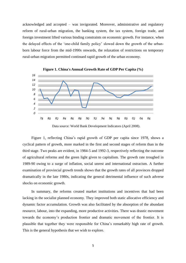
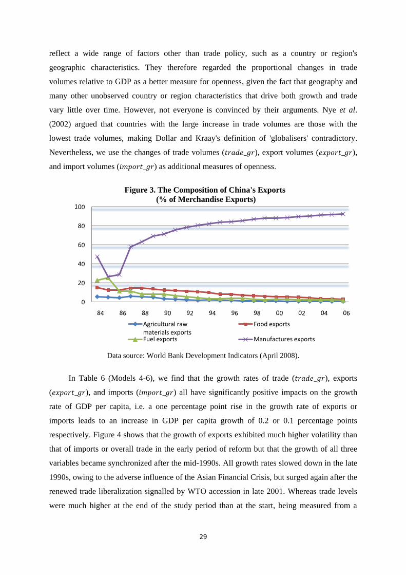
Data source: World Bank Development Indicators (April 2008).
Figure 1, reflecting China’s rapid growth of GDP per capita since 1978, shows a
cyclical pattern of growth, more marked in the first and second stages of reform than in the
third stage. Two peaks are evident, in 1984-5 and 1992-3, respectively reflecting the outcome
of agricultural reforms and the green light given to capitalism. The growth rate troughed in
1989-90 owing to a surge of inflation, social unrest and international ostracism. A further
examination of provincial growth trends shows that the growth rates of all provinces dropped
dramatically in the late 1980s, indicating the general detrimental influence of such adverse
shocks on economic growth.
In summary, the reforms created market institutions and incentives that had been
lacking in the socialist planned economy. They improved both static allocative efficiency and
dynamic factor accumulation. Growth was also facilitated by the absorption of the abundant
resource, labour, into the expanding, more productive activities. There was drastic movement
towards the economy’s production frontier and dramatic movement of the frontier. It is
plausible that together they were responsible for China’s remarkably high rate of growth.
This is the general hypothesis that we wish to explore.
0
2
4
6
8
10
12
14
16
Figure 1. China's Annual Growth Rate of GDP Per Capita (%)

6
3. The growth literature on China
The starting point in this research is our paper utilising cross-country data to estimate
an augmented Solow model of economic growth (Ding and Knight, 2008a). Our estimated
growth equations were used to predict China’s performance. By inserting China’s values of
the explanatory variables in the equation, we found that the growth rate could indeed be well
explained. Five factors – conditional convergence from a low income level, high physical
capital formation, high level of human capital, rapid structural change away from agriculture,
and slow population growth – made the main contributions to the difference between China’s
growth and that of other developing regions. By providing these pointers, this cross-country
analysis sets the scene for the current cross-province analysis.
There is a large literature on cross-province growth regressions for China3. Two
empirical approaches have been used: some version of the neoclassical growth model, often
in the form of the augmented Solow model as developed by Mankiw, Romer and Weil (1992)
(MRW), or informal growth regressions (for instance, Barro, 1991; Barro and Sala-i-Martin,
2004), that contain among others the explanatory variables in which the researcher is most
interested. Different periods are analysed, although most are confined to the period of
economic reform, from 1978 onwards. The methods of analysis vary in sophistication, from
cross-section OLS to panel data GMM analysis. Research focus covers a broad range of
factors relating to variation in growth among Chinese provinces, such as convergence or
divergence, physical and human capital investment, openness, economic reform,
geographical location, infrastructure, financial development, labour market development,
spatial dependence and preferential policies. An underlying problem in all the research is the
need to find causal relationships as opposed to mere associations.
Both Chen and Fleisher (1996) and Li et al. (1998) discovered that China's economic
growth over the reform period generated significant forces for convergence of both provincial
levels and growth rates of GDP per capita. The convergence was conditional on the variables
controlling for the steady state in the augmented Solow model. The levels and growth rates of
GDP per capita were higher in the provinces with lower population growth, more investment
in physical and human capital and greater openness to foreign countries. Raiser (1998) and
Zhang (2001) investigated both and convergence across Chinese provinces and found
that the rate of convergence declined after 1985, which decline they attributed to the shift
3 The literature survey does not include growth accounting or time-series aggregate growth regressions for
China.

7
from rural to urban reforms, the reduction of inter-provincial fiscal transfers, and different
opportunities for international trade and foreign direct investment (FDI).
Yao (2006) examined the effect of exports and FDI on provincial growth rates over the
period 1978-2000. By adopting Pedroni's panel cointegration test and Arellano and Bond's
dynamic panel data estimating technique to control for the problems of non-stationarity and
endogeneity, he found that both exports and FDI made a positive and significant contribution.
He established the existence of simultaneous relationship between FDI and GDP growth and
between exports and GDP growth, and concluded that the interaction among these three
variables formed a virtuous circle of openness and growth in China.
Chen and Feng (2000) adopted a Barro-type framework to model the determinants of
cross-province variation in economic growth over the period 1978-89. Their intention was to
investigate the commonalities among China's and other countries' growth patterns as well as
China's unique growth characteristics. They found that university education, industrialization
and international trade raise growth, whereas high fertility and high inflation reduce it. A
China-specific institutional factor, the presence of SOEs, was found to inhibit growth.
Bao et al. (2002) investigated the effect of geography on regional economic growth in
China under market reforms and found that geographic factors such as coastline length,
distance factor and population density close to the coastline are important in explaining
growth disparities across provinces. Brun et al. (2002) focused on the spillover effects of
economic growth from China's coastal to non-coastal regions and found that spillover effects
were not sufficient to reduce income disparities among the provinces.
Démurger (2001) assessed the relationship between infrastructure development and
economic growth in China. The fixed-effect and two-stage least-squares results showed that
differences in geographical location, transport infrastructure and telecommunication facilities
accounted for a significant part of the observed differences in growth performance across
provinces.
Hao (2006) examined the impact of the development of financial intermediation on
growth over the period 1985-99 and found that it contributed to China's economic growth
through two channels: the substitution of loans for state budget appropriation and the
mobilization of household savings. Loan expansion itself did not contribute to growth
because the distribution of loans, not being based on commercial criteria, was inefficient.
Guariglia and Poncet (2006) showed that financial distortions represented an impediment to

8
economic growth in China over the period 1989-2003, i.e. traditional indicators of financial
development and China-specific indicators of state intervention are generally negatively
associated with growth and its sources, whereas indicators of market-driven financing are
positively correlated with them. The adverse effects of financial distortions on growth have
gradually declined over time, possibly owing to the progressive reform of the banking sector
especially after China's entry to the WTO in 2001. They argued that FDI is an important
factor in alleviating the costs of financial distortions, so suggesting a partial explanation for
why China can grow fast despite a malfunctioning financial system.
Cai et al. (2002) placed emphasis on the impact of lagged labour market reform on
increasing regional disparity in China during the period 1978-98. They used the comparative
productivity of agricultural labour as a proxy for labour market distortion and found that this
measure impedes regional growth rates after controlling for a set of variables determining the
steady state.
Jones et al. (2003) tested the augmented Solow model using city-level data for the
decade 1989-99. They showed that policies giving preferential treatment to cities by
promoting openness, such as special economic zone status or open coastal status, accounted
for a large part of the differences in growth rates across cities. These policies affected growth
directly by creating an environment more conducive to production, and indirectly by
encouraging FDI to flow to these cities. Higher rates of FDI and lower rates of population
growth were shown to be related to faster growth of per capita income. Surprisingly, they
found no evidence for a positive effect of domestic investment on city growth, their
explanation being that domestic investment in China is not primarily profit-driven and is thus
inefficiently allocated.
These studies often use an assortment of economic theories to motivate a variety of
variables that are included in the cross-province or cross-city growth regressions, and then
test the robustness of their conclusions to the addition of an ad hoc selection of further
controls. Although each study presents intuitively appealing results, none has directly posed
the general question: can the variations among provinces highlighted by cross-province
growth regressions explain why the economy as a whole has grown so fast? Moreover, no
systematic consideration has been given to uncertainty about the regression specification,
with the implication that conventional methods for inference can be misleading. We therefore
attempt to fill these two gaps in the growth literature on China by using some recently

9
developed methods of model selection. The baseline model will then be used to examine the
deeper causes of rapid economic growth.
4. Empirical methodology and data
4.1 Empirical methods
There is no single explicit theoretical framework to guide empirical work on economic
growth. The neoclassical model (Solow, 1956) predicts that the long-run economic growth
rate is determined by the rate of exogenous technological progress, and that adjustment to
stable steady-state growth is achieved by endogenous changes in factor accumulation. It is
silent on the determinants of technological progress. Endogenous growth theory (for instance,
Lucas, 1988; Romer, 1990) concentrates on technological progress and emphasizes the role
of learning by doing, knowledge spillover, research and development, and education in
driving economic growth. Because the theories are not mutually exclusive, the problem of
model uncertainty concerning which variables should be included to capture the underlying
data generating process presents a central difficulty for empirical growth analysis. This issue
has gained increasing attention in the cross-country growth literature following the seminal
work of Barro (1991), which identified a wide range of variables that are partially correlated
with GDP per capita growth. A number of econometric and statistical methodologies have
been developed and applied to handle model uncertainty, among which the Extreme Bounds
Analysis, Bayesian Model Averaging, and General-to-Specific approach are most influential.
The issue of fragility of econometric inference with respect to modelling choices was
first addressed by Leamer (1983, 1985), who proposed an Extreme Bounds Analysis (EBA)
to test for the sensitivity of estimated results with respect to changes in the prior distribution
of parameters. The extreme bounds for the coefficient of a particular variable are defined as
the lowest estimate of its value minus two times its standard error and the highest estimate of
its value plus two times its standard error when different combinations of additional
regressors enter the regression. A variable is regarded to be robust if its extreme bounds lie
strictly to one side or the other of zero, i.e. the coefficient of interest displays small variation
to the presence or absence of other regressors.
Levine and Renelt (1992) applied this methodology to cross-country growth regressions
and investigated the robustness of a large number of variables that were found in the
literature to be correlated with growth. In order to reduce the number of regressions required
to compute the extreme bounds, they imposed several restrictions on the conditioning

10
information set in modelling, for instance, four variables are always included in every
regression based on past empirical studies and economic theory4; up to only three other
control variables can be selected each time from a large pool of variables potentially
important for growth. Using this variant version of EBA, they found that very few variables
are robustly correlated with growth, i.e. almost all results are fragile to changes in the list of
conditioning variables. The only exception is a positive and robust correlation between
growth and the share of investment in GDP.
Sala-i-Martin (1997) challenged their pessimistic finding by adopting a less restrictive
sensitivity test for the explanatory variables in the growth regressions. He claimed that the
version of Levine and Renelt (1992) of EBA is too strong for any variable to pass; for
instance, a single irrelevant outlier of the distribution of the coefficient estimates may make
the variable non-robust. Therefore, rather than simply classifying variables as robust or
fragile, Sala-i-Martin (1997) attempted to assign some level of confidence to each of the
variables by computing the entire cumulative distribution function of the estimates of the
variable of interest5. In this case, a variable is regarded to be robust if 95 percent of the
distribution of the coefficient estimates lies to one or the other side of zero. In addition, Sala-
i-Martin (1997) made a persuasive case that several of the variables chosen by Levine and
Renelt (1992) are almost certainly endogenous. Instead he assembled a dataset that was less
susceptible to that problem. Not surprisingly, a substantial number of variables turn out to be
strongly related to economic growth using this method.
One potential shortcoming of the approach used by Sala-i-Martin (1997) is that, owing
to the lack of statistical theory, the statistical properties of the computed weighted averages
are not well understood. To solve this problem, Fernández et al. (2001) and Sala-i-Martin et
al. (2004) adopted an alternative technique, Bayesian Model Averaging (BMA), to re-
examine the Sala-i-Martin (1997) dataset, in which model uncertainty is addressed using a
formal statistical approach. The basic idea of BMA is that the posterior distribution of any
parameter of interest is a weighted average of the posterior distributions of that parameter
under each of the models with weights given by the posterior model probabilities, following
strictly the rules of probability theory (see, for example, Leamer, 1978). Unlike the
approaches which restrict the set of regressors to contain certain fixed variables and then add
4 They are the investment share of GDP, the initial level of real GDP per capita in 1960, the initial secondary
school enrolment rate and the average rate of population growth. 5 He constructed the weighted averages of all the estimates of the variable of interest and its corresponding
standard deviations, using weights proportional to the likelihoods of each of the models.
11
a small number of other variables, BMA allows for any subset of the variables to appear in
the model. Fernández et al. (2001) set out a full BMA framework, which requires the
specification of the prior distribution of all of the relevant parameters conditional on each
possible model. Based on theoretical results and extensive simulations, they used the so-
called 'improper uninformative priors' for the parameters, which are designed to be relatively
uninformative so that, given informative data, the final results place relatively little weight on
subjective prior knowledge. However, Sala-i-Martin et al. (2004) argued that acquisition of
prior parameter information is difficult and sometimes infeasible when the number of
possible regressors is large. Instead, they proposed a method of Bayesian Averaging of
Classical Estimates (BACE), which assumes diffuse priors for the parameters, and for which
only one prior parameter specification, the expected model size, is required. Both versions of
BMA broadly support the more optimistic conclusion of Sala-i-Martin (1997) that a good
number of economic variables have a robust partial correlation with long-run growth.
Another strand of research on model uncertainty is the General-to-Specific (GETS)
search methodology emphasized by Hendry and Krolzig (2004). The basic idea is to specify a
general unrestricted model (GUM), which is assumed to characterize the essential data
generating process, and then to 'test down' to a parsimonious encompassing and congruent
representation based on the theory of reduction. They claimed that using the GETS approach
permits them to replicate most of the findings of Fernández et al. (2001) in just a few
minutes. The huge efficiency gain makes the automatic procedures of model selection
extremely attractive. Hoover and Perez (2004) compared the performance of the GETS
approach with EBA adopted by Levine and Renelt (1992) and Sala-i-Martin (1997). Their
Monte Carlo simulation results indicate that GETS algorithm not only usually finds the truth
but also discriminates between true and false variables extremely well. By contrast, EBA in
the form advocated by Levine and Renelt (1992) is too stringent and rejects the truth too
frequently, while that advocated by Sala-i-Martin (1997) is not able to discriminate and
accepts the false too frequently along with the true. According to Hoover and Perez (2004),
Sala-i-Martin (1997) was right to criticize Levine and Renelt (1992) for rejecting too many
potential determinants of growth as non-robust, but his approach selected many variables that
probably do not truly determine differences in growth rates among countries. They therefore
concluded that GETS method is superior to EBA in getting at the truth.
In this paper we adopt both BMA and GETS approaches to consider the association
between GDP per capita growth rates and a wide range of potential explanatory variables

12
based on the cross-sectional data. The purpose of the first-stage model selection is to provide
guidance on the choice of variables to include in the subsequent panel data analysis. BMA
and GETS procedures have comparative advantages in dealing with model uncertainty and
allow us to consider a wide range of candidate predictors in a rigorous way. However, neither
of them is without limits nor immune from criticism. For example, one key disadvantage of
BMA is the difficulty of interpretation, i.e. parameters are assumed to have the same
interpretation regardless of the model they appear in; in addition, it does not lead to a simple
model, making the interpretation of results harder (Chatfield, 1995). Criticisms of GETS
modelling are commonly concerned with the problems of controlling the overall size of tests
in a sequential testing process and of interpreting the final results from a classical viewpoint
(Owen, 2003). Hence, the joint application of BMA and GETS model selection procedures in
this paper is to combine the strengths of both methods and to circumvent the limitations of
each to some extent (see Appendix 1 for brief discussion of the two methods).
Owing to the inclusion of potentially endogenous variables, no causal interpretation is
attached to the results at this stage. When a subset of variables are identified as receiving the
greatest support from the underlying data according to the model selection results, a further
panel data analysis is conducted to investigate the deeper determinants of provincial GDP per
capita growth in China. Although cross-sectional regression has the advantage of focusing on
the long-run trends of economic growth, panel data methods can control for omitted variables
that are persistent over time, and can alleviate measurement error and endogeneity biases by
use of lags of the regressors as instruments (Temple, 1999).
We use a system GMM estimator, developed by Arellano and Bover (1995) and
Blundell and Bond (1998), which combines the standard set of equations in first-differences
with suitably lagged levels as instruments, with an additional set of equations in levels with
suitably lagged first-differences as instruments. By adding the original equation in levels to
the system, they found dramatic improvement in efficiency and significant reduction in finite
sample bias through exploiting these additional moment conditions. Bond et al. (2001) also
claimed that the potential for obtaining consistent parameter estimates even in the presence of
measurement error and endogenous right-hand-side variables is a considerable strength of the
GMM approach in the context of empirical growth research. Finally, the robustness of our
selected models and the contribution of main variables are carefully examined. In this paper
we concentrate on the role of openness, institutional change and sectoral change in driving
China's economic growth.

13
4.2 The dataset
The original sample consists of a panel of 30 provinces with annual data for the period
1978-20066
. The data come mainly from China Compendium of Statistics 1949-2004
compiled by National Bureau of Statistics of China. The data of 2005 and 2006 are obtained
from the latest issues of China Statistical Yearbook. The reliability of Chinese official
macroeconomic data is often under dispute7. One important issue is the problem of data
inconsistency over the sample period. For example, GDP figures for the years 2005 and 2006
were recompiled on the basis of China's 2004 Economic Census, while corresponding
provincial data for earlier years remain unrevised. Another problem is data non-comparability
across provinces. Take population as an example: the household registration population
figure is provided for some provinces, whereas for others only permanent population data are
available. In addition, the substantial 'floating population' of temporary migrants is not fully
accounted for by the population data. These discrepancies can result in measurement error
problems and may call into question the reliability of our estimation results. Therefore, on the
one hand, we use a number of 'cleaning rules' (see Appendix 3) to get rid of potential outliers
for each variable and, on the other hand, we employ the panel data System GMM estimator to
deal with potential mismeasurement.
Our first-stage model selection analysis is based on cross-sectional data, in which
observations are averaged over the entire sample period. For the subsequent panel-data study,
we opt for the non-overlapping five-year time interval, which is widely used in the cross-
country growth literature (for instance, Islam, 1995; Bond et al., 2001; Ding and Knight,
2008a). On the one hand, by comparison with the yearly data, the five-year average setup
alleviates the influence of temporary factors associated with business cycles. On the other
hand, we are able to maintain more time series variation than would be possible with a
longer-period interval.
All the variables are calculated in 1990 constant prices and price indices are province-
specific8. The dependent variable is the growth rate of real GDP per capita. Table 1 shows
descriptive statistics of provincial growth rates of real GDP per capita. The annual average
6 China is administratively decomposed into 31 provinces, minority autonomous regions, and municipalities.
Since Chongqing becomes a municipal city since 1997, we combine Chongqing with Sichuan for the period
1997-2006, so making it consistent with earlier observations .
7 Influential work on the (un)reliability of China's GDP statistics includes Maddison (1998), Rawski (2001),
Lardy (2002), Young (2003) and Holz (2006). 8 The deflator is the provincial consumer price index. The provincial price data of Tibet are missing for the
period 1978-89; we use the national aggregate price index to substitute.

14
per capita growth rates of all 30 provinces over the entire reform period was 7.6 percent, with
an average value of 8.2 percent for the coastal provinces and 7.2 percent for interior
provinces. China's economic reform generated across-the-nation rapid growth, i.e. both the
coastal and inner regions grew fast by international standards. However, that a growth
disparity did exist is indicated by the five-percent average growth difference between the
highest growth province (Zhejiang) and lowest one (Gansu) over the full sample period.
Table 1 also reveals interesting time patterns in China's growth. Rapid growth occurred in the
first decade, slowed down and became more volatile in the second decade, and accelerated
but stabilized in the third decade. In the period 1998-2006, the growth disparity across
provinces became smaller and even the lowest-growing province (Yunnan) managed an
average rate of 7.9 percent.
Table 1. Descriptive Statistics of Provincial GDP Per Capita Growth Rates
Full-sample period Sub-sample periods
1978-2006 1978-1987 1988-1997 1998-2006
All provinces (30 provinces) 0.076
(0.058)
0.073
(0.056)
0.054
(0.065)
0.102
(0.037)
Coastal provinces (11 provinces) 0.082
(0.058)
0.076
(0.053)
0.065
(0.071)
0.105
(0.032)
Interior provinces (19 provinces) 0.072
(0.058)
0.071
(0.058)
0.047
(0.060)
0.100
(0.039)
Highest growth province 0.102
(0.061)
0.112
(0.057)
0.108
(0.075)
0.119
(0.042)
Lowest growth province 0.055
(0.060)
0.020
(0.025)
0.012
(0.089)
0.079
(0.036)
Note: Mean values and standard deviations (in parentheses) are provided; coastal provinces consist of
Liaoning, Hebei, Tianjin, Shandong, Jiangsu, Shanghai, Zhejiang, Fujian, Guangdong, and Hainan, plus
Beijing; and interior provinces include Anhui, Gansu, Guangxi, Guizhou, Heilongjiang, Henan, Hubei,
Hunan, Inner Mongolia, Jiangxi, Jilin, Ningxia, Qinghai, Shaanxi, Shanxi, Sichuan, Tibet, Xinjiang and
Yunnan; for the full-sample period, the highest growth province was Zhejiang, and the lowest growth
province was Gansu; for the three sub-sample periods, Zhejiang, Fujian, Shandong were the highest growth
provinces respectively, and Shanghai, Tibet, Yunnan were the corresponding lowest growth provinces.
The explanatory variables can be broadly classified into ten categories: initial level of
income, physical capital formation, human capital formation, population growth rate, degree
of openness, pace of economic reform or institutional change, sectoral change, infrastructure,
financial development, and geographic location (see Appendix 3 for detailed definitions).
5. Empirical results of baseline equation
15
5.1 First-stage model selection results
The validity of a selected model depends primarily on the adequacy of the general
unrestricted model as an approximation to the data generation process (Doornik and Hendry,
2007). A poorly specified general model stands little chance of leading to a good 'final'
specific model. We consider ten different groups of explanatory variables, and rely on theory
of economic growth (although sufficiently loose) and previous empirical findings to guide the
specification of the general model. One important issue is that variables within each category
are highly correlated, which may result in the problem of multicollinearity and thus inflate
the coefficient standard errors if all variables are simultaneously included in one general
regression. The strategy we adopt is to select one or two representative variables from each
range (based on existing empirical literature and correlation results) to form the basic general
model, and then to test for the robustness of the model selection results using other variables
left in each group. Throughout this section, when we refer to growth we shall, unless
indicated otherwise, mean annual average growth of real GDP per capita.
We start from a general model that includes 13 explanatory variables and searches for
statistically acceptable reductions of this model. The included variables are the logarithm of
initial level of income ( ), ratio of fixed capital formation over GDP ( ),
secondary school enrolment rate ( ), ratio of students enrolled in higher education
to students enrolled in regular secondary education ( ), population natural
growth rate ( ), ratio of exports to GDP ( ), SOEs' share of total industrial
output ( ), change in non-agricultural share of employment ( ),
degree of industrialization ( ), railway density ( ), ratio of business
volume of post and telecommunications to GDP ( ), and a coastal dummy
( ).
The correlation matrix of these variables is presented in Table 2. The positive
correlation between growth and initial level of income suggests that there exists absolute
(unconditional) divergence, rather than convergence, across the provinces over the entire
sample period. Formal regression analysis using five-year average panel data system GMM
shows similar results (Table 5): regressing the growth rate of GDP per capita on the
logarithm of initial income term alone yields a positive and significant coefficient. In the
growth literature, it is commonly believed that absolute convergence is more likely to apply
across regions within countries than across countries because the former tend to have similar
institutional arrangements, legal systems and cultures, giving rise to the possibility of their

16
Table 2. Correlation Matrix of the General Model
1.0000
0.3081 1.0000
0.4081 0.5010 1.0000
0.4147 0.5134 0.3645 1.0000
0.2943 0.7520 0.4465 0.3341 1.0000
-0.4350 -0.7942 -0.3482 -0.5435 -0.6691 1.0000
0.1992 0.6319 0.1539 0.2085 0.4495 -0.3600 1.0000
-0.5287 -0.6915 -0.3504 -0.3978 -0.3940 0.6884 -0.4881 1.0000
0.2666 -0.0246 0.0038 -0.0366 -0.0811 0.0285 0.1282 -0.0527 1.0000
0.1077 0.6512 0.1398 0.3677 0.5552 -0.5904 0.5296 -0.3604 0.0440 1.0000
0.0091 0.4758 0.1461 0.2296 0.6114 -0.4482 0.3539 -0.1709 -0.1408 0.5666 1.0000
0.5871 0.6663 0.6803 0.5524 0.5613 -0.5986 0.3393 -0.6854 -0.0055 0.2234 0.1231 1.0000
0.1783 0.3889 0.5121 0.1388 0.4140 -0.2781 0.1874 -0.1703 -0.0074 0.2545 0.1743 0.4563 1.0000
0.0976 0.4791 -0.0323 0.0792 0.3360 -0.3351 0.5801 -0.3379 0.1477 0.4465 0.4204 0.0405 0.0098 1.0000

17
convergence to the same steady state. For instance, Barro and Sala-i-Martin (2004) found
evidence that absolute convergence is the norm for the US states since 1880, the prefectures
of Japan since 1930, and the regions of eight European countries since 1950. By contrast,
some researchers have argued that heterogeneity in technology, preferences, and institutions
may prevent unconditional convergence from occurring across regions (for example,
Beenstock and Felsenstein, 2008). Our finding of unconditional regional divergence in China
supports the latter view. Among other variables, only population growth and SOEs' share of
total industrial output show a strong negative correlation with growth, which is consistent
with our predictions.
We first use BMA to isolate variables that have a high posterior probability of
inclusion. In Table 3, we present a summary of the BMA results, where the posterior
probability that the variable is included in the model, the posterior mean, and the posterior
standard deviation for each variable are reported. We are aware of the difficulty of
interpreting parameters in economic terms when the conditioning variables differ across
models, so our emphasis here lies on the posterior probability of inclusion for each variable,
i.e. the sum of posterior model probabilities for all models in which each variable appears.
The results indicate a possibly important role for the initial level of income, SOEs' share of
total industrial output, secondary school enrolment rate, coastal dummy, exports, fixed capital
formation, and population growth. Each of these variables has a posterior probability of
inclusion above 25 percent.
Table 3. Bayesian Model Averaging (BMA) Results
Regressor Posterior Probability
of Inclusion
Posterior
Mean
Posterior Standard
Deviation
100.0 0.207 0.042
100.0 -0.019 0.007
96.9 -0.053 0.022
93.4 0.352 0.175
62.2 0.006 0.006
29.7 0.011 0.022
29.3 0.015 0.029
27.8 -0.432 0.904
24.8 0.017 0.039
10.8 -0.001 0.006
7.8 -0.006 0.041
7.3 0.001 0.006
5.4 0.009 0.123
4.3 -0.002 0.022
Notes: Estimation is based on cross-sectional data; Dependent variable: growth rate of real
provincial GDP per capita.

18
We then conduct an automatic model selection exercise using the GETS methodology.
Starting from the same general model and searching for statistically acceptable reductions,
Autometrics arrives at a final model with a set of explanatory variables broadly similar to
those highlighted by the BMA analysis. The OLS estimation of the final specific model is
reported in Table 4. We find that the initial income level, population growth and SOEs' share
of industrial output are negatively correlated with GDP per capita growth, whereas fixed
capital investment, secondary school enrolment rates and exports are positively correlated.
The major difference between the results of the two methods lies in the role of the regional
dummy variable in explaining cross-province growth rates, i.e. BMA analysis flags the
coastal dummy as potentially important (with a posterior inclusion probability of 62 percent),
but GETS drops that variable during reductions. Other variables such as sectoral change,
infrastructure and financial development are flagged as unimportant predictors of economic
growth by both model selection methods. However, this outcome may simply reflect the
highly endogenous nature of these variables, which cannot be accounted for at the model-
selection stage. We will re-examine the role of these variables in determining output growth
in the panel data context later.
Table 4. General-to-Specific (GETS) Model Selection Results
Regressor Coefficient Standard
Error t-value t-probability Part.
0.248 0.038 6.515 0.000 0.649
-0.025 0.006 -4.307 0.000 0.447
0.059 0.027 2.234 0.036 0.178
0.309 0.147 2.104 0.047 0.161
-1.854 0.891 -2.082 0.049 0.159
0.041 0.021 1.934 0.066 0.139
-0.056 0.018 -3.134 0.005 0.299
Sigma 0.007 RSS 0.001 0.767
F(6,23) 12.64 [0.000] LogLik 108.627 T 30
AIC -9.613 SC -9.286 HQ -9.508
Normality test
Chi^2(2) = 1.872 [0.393]
Testing for heteroscedasticity F(12,10) = 0.558 [0.832]
Notes: This is the OLS estimation of final specific model based on cross-sectional data; Dependent
variable: growth rate of real provincial GDP per capita.
5.2 Second-stage panel data results
The existence of a robust partial correlation does not imply that the variables of interest
cause growth (Levine and Renelt, 1992). Based on the model selection results delivered by
19
BMA and GETS, we therefore estimate the baseline model using panel data system GMM, in
which the endogeneity of regressors can be controlled for. Note that all estimated standard
errors are corrected for heteroscedasticity and that time dummies are included. We treat the
population natural growth rate as an exogenous variable, the initial level of income as a
predetermined variable, and all other variables including physical and human capital
accumulation, exports and SOEs' share of industrial output as potentially endogenous
variables. Since the p values of over-identifying tests may be inflated when the number of
moment conditions is large (Bowsher, 2002), we restrict the number of instruments used for
each first differenced equation by including a subset of instruments for each predetermined or
endogenous variable. Several studies have found that the two-step standard errors tend to be
biased downwards in finite samples (Arellano and Bond, 1991; Blundell and Bond, 1998). By
applying a correction to the two-step covariance matrix derived by Windmeijer (2005), we
find very similar results obtained from the one-step and two-step GMM estimators. To
conserve space we report only the heteroscedasticity-robust one-step system GMM results.
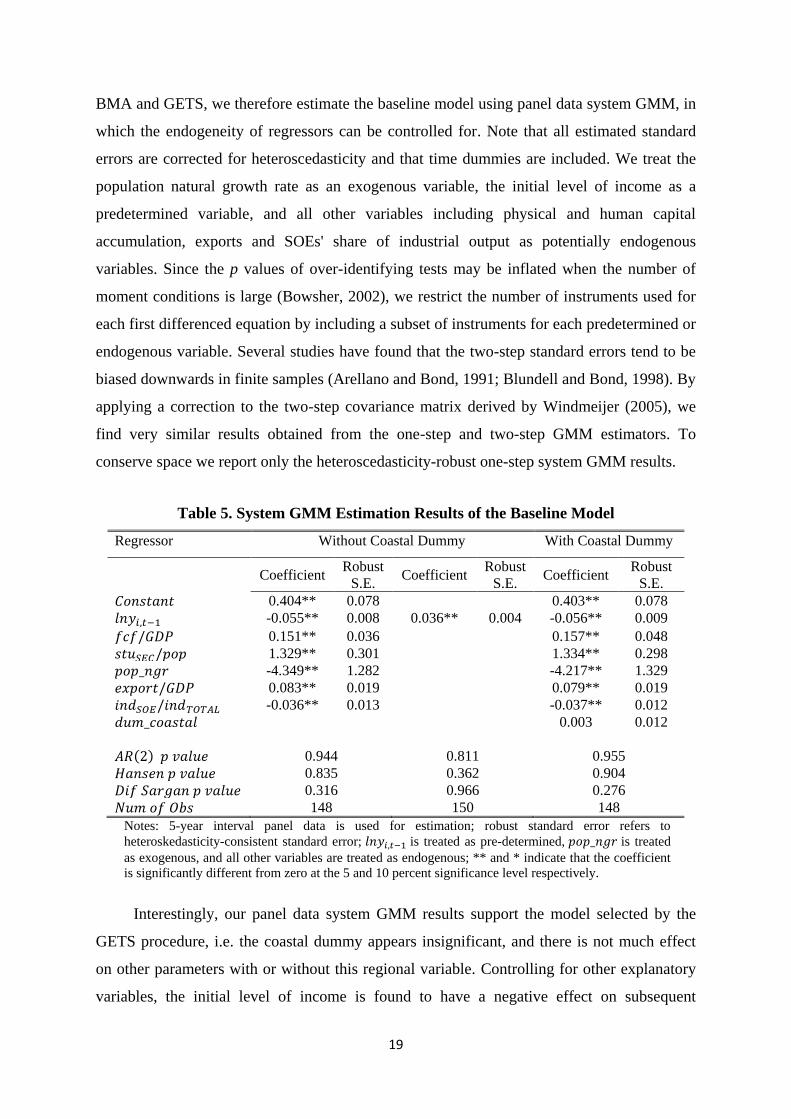
Table 5. System GMM Estimation Results of the Baseline Model
Regressor Without Coastal Dummy With Coastal Dummy
Coefficient Robust
S.E. Coefficient
Robust
S.E. Coefficient
Robust
S.E.
0.404** 0.078 0.403** 0.078
-0.055** 0.008 0.036** 0.004 -0.056** 0.009
0.151** 0.036 0.157** 0.048
1.329** 0.301 1.334** 0.298
-4.349** 1.282 -4.217** 1.329
0.083** 0.019 0.079** 0.019
-0.036** 0.013 -0.037** 0.012
0.003 0.012
0.944 0.811 0.955
0.835 0.362 0.904
0.316 0.966 0.276
148 150 148
Notes: 5-year interval panel data is used for estimation; robust standard error refers to
heteroskedasticity-consistent standard error; is treated as pre-determined, is treated
as exogenous, and all other variables are treated as endogenous; ** and * indicate that the coefficient
is significantly different from zero at the 5 and 10 percent significance level respectively.
Interestingly, our panel data system GMM results support the model selected by the
GETS procedure, i.e. the coastal dummy appears insignificant, and there is not much effect
on other parameters with or without this regional variable. Controlling for other explanatory
variables, the initial level of income is found to have a negative effect on subsequent
20
provincial growth rates, providing evidence of conditional convergence over the reform
period. The estimated coefficient implies that a one percent lower initial level of GDP per
capita raises the subsequent growth rate of GDP per capita by 0.06 percentage points.
Conditional convergence is an implication of the neoclassical growth model, deriving from
the assumption of diminishing returns to capital accumulation. The controls imply that the
provinces have different steady states, and that convergence will lead them to their respective
steady state levels of income per capita. Despite the challenge posed by endogenous growth
theory, the neoclassical paradigm of convergence is widely supported by empirical evidence
in both the cross-country growth literature (for example, MRW, 1992; Islam, 1995; Bond et
al., 2001; Ding and Knight, 2008a) and the cross-province growth study on China (for
example, Chen and Fleisher, 1996; Chen and Feng, 2000; Cai et al., 2002). Table 5 also
shows estimates of the effects of initial income per capita in the absence of controls for other
variables: the coefficient is significantly positive, indicating absolute divergence.
Our findings of absolute divergence and conditional convergence reveal an interesting
growth pattern in China: poor provinces did not grow faster than rich ones, but they tended to
converge in a relative sense towards their own steady states. One possible explanation for this
pattern is that relatively poor provinces have lower stocks of physical and human capital, so
that the marginal product of capital is higher for them. Another explanation might lie in
central government's regional development policies. During the period 1978-1993, fiscal
decentralization reform gave provincial governments more discretionary power in tax
administration and revenue collection. The 'fiscal contracting system' reduced central
government's share of revenue and curtailed fiscal transfers away from rich and towards poor
provinces (Raiser, 1998; Knight and Li, 1999). In 1994, the 'tax assignment system' reform
strengthened central government's fiscal capacity, which enabled it to increase fiscal
redistribution towards poor provinces and to promote economic development in poor regions
such as the western provinces and minority areas. This might help to explain why absolute
divergence has been weaker in recent years (Table 1).
Fixed capital formation is an important determinant of China's growth, i.e. a one
percentage point rise in the ratio of fixed capital formation to GDP in a province raises its
growth rate of GDP per capita by 0.2 percentage points. Human capital investment appears to
be even more important, i.e. a one percentage point increase in secondary school enrolment
rates is associated with a higher growth rate of GDP per capita by 1.3 percentage points.
21
More detailed investigation of the growth impacts of physical and human capital
accumulation was conducted in a companion paper (Ding and Knight, 2008a).
Natural increase in population has a negative consequence for growth, i.e. reducing the
rate of population growth by one percent is associated with an increase in GDP per capita
growth of 0.5 percent9. Rapid population growth rate can be referred to as an opportunity cost
of economic growth, i.e. faster growth of the labour force means more capital has to be used
to equip the growing labour force, and hence there is less scope for capital deepening, with
resultant slower growth of capital per worker and thus output per worker. From the
neoclassical point of view and within the standard Solow model, slower population growth
implies a higher equilibrium level of the output per worker and capital stock per worker. This
means that a province is further from its equilibrium and the forces of convergence are
therefore stronger, so raising the output per worker faster. China has been keen to curb its
population growth mainly through the family planning policy, implemented since the late
1970s. Despite the controversy over the humanity of the 'one-child family policy', such
tightened demographic policy has been efficient in slowing down population growth and
reducing the strain on resources in China, which has a positive impact on its growth of GDP
per capita.
Exports are conducive to provincial growth, i.e. a one percentage point increase in the
ratio of exports to GDP leads to an increase in GDP per capita growth of 0.08 percentage
points. According to the report of Commission on Growth and Development (2008), a
flourishing export sector is an important ingredient of high and sustained growth, especially
in the early stages. In endogenous growth theory, international trade, especially exports, is
viewed as an important source of human capital augmentation, technological change and
knowledge spillover across countries (Grossman and Helpman, 1995). China's open-door
policy, adopted after 1978, created an excellent opportunity to exploit its comparative
advantage in the labour-intensive manufacturing industry, making exports a driver of China's
growth.
The SOEs' share of industrial output has a significant and negative impact on output
growth, i.e. a decrease of one percentage point in the variable raises GDP per capita growth
rate by 0.04 percentage points. This variable is a proxy for the pace of economic reform or
institutional change. In the mid-1980s, SOEs were given successively greater autonomy in
9 We calculate the elasticity of with respect to , equivalent to .
22
production and a greater share of the profits they generated through a variety of profit
remittance contracts and management responsibility systems (Riedel et al., 2007). However,
owing to the principal-agent problem inherent to state ownership, the effect of the industrial
reform in improving the efficiency and profitability of SOEs remained limited. By contrast,
non-state-owned enterprises such as collectively-owned rural township and village
enterprises in the 1980s and domestic and foreign privately-owned industrial enterprises in
the 1990s grew rapidly in response to market opportunities and better incentive structures.
Therefore, the declining share of SOEs in industrial output is conducive to the growth of
GDP per capita.
Our system GMM estimation shows that there is no evidence of second order serial
correlation in the first-differenced residuals and neither the Hansen test nor the Difference
Sargan test rejects the validity of instruments, all of which results suggest the consistency of
the estimators being used. In brief, our panel data results favour the model selected by GETS
procedure and highlights the role of conditional convergence, physical and human capital
formation, population growth, degree of openness, and institutional change in determining
economic growth across Chinese provinces.
6. Degree of openness
6.1 Brief literature survey on the openness-growth nexus
In this section, we examine the role of openness to trade and to foreign direct
investment in accelerating China's growth. In trade theory, the static effect of openness on the
level of income can arise from specialization according to comparative advantage,
exploitation of increasing returns, and spread of technology and information. The effect of
openness on the rate of growth is widely addressed in the endogenous growth literature (see,
for example, Romer, 1990; Grossman and Helpman, 1990). If greater competition or
exposure to new technologies and ideas were to increase the rate of technological progress, it
would permanently raise the growth rate (Winters, 2004). The channels through which
openness affects economic growth may lie in access to the technological knowledge of trade
partners or foreign investors and to markets with new products and inputs, transfer of
multinational enterprises' managerial expertise, and greater R&D through increasing returns
to innovation. It is difficult to judge empirically whether faster growth is a transitional or a
permanent effect. In any case, since much empirical and theoretical work (for instance,
Mankiw et al., 1992; Hall and Jones, 1997; Barro and Sala-i-Martin, 2004; Dollar and Kraay,

23
2004; Ding and Knight, 2008a) suggests that transitional dynamics may take several decades,
our research focus on growth rather than on income is appropriate.
The hypothesis that openness is a positive force for growth has been examined in
numerous cross-country studies. For example, Dollar (1992) found that a measure of outward
orientation, based on real exchange rate distortion and variability, is highly positively
correlated with GDP per capita growth in a sample of 95 developing countries. Sachs and
Warner (1995) concluded that open economies, defined by absence of five conditions,
experienced an average annual growth rate of 2 percent above that of closed economies in the
period 1970-89, and that convergence only occurred in the sample of open countries.
Edwards (1998) adopted nine alternative openness indices to analyse the connection between
trade policy and productivity growth during the period 1980-90, and showed that openness
contributed to faster TFP growth. Using geographic factors as an instrument for trade
volume, Frankel and Romer (1999) examined causality between trade and income level as
well as the channels through which trade affects subsequent income. They found that trade
does indeed have a quantitatively large and robust positive effect on income.
Empirical research on the openness-growth link faces at least three problems. Firstly,
the appropriate definition of openness depends on the precise hypothesis to be tested, in this
case the effect of openness, or its change, on growth. Secondly, it is difficult to measure
openness. Pritchett (1996) pointed out that any single measure is unlikely to capture the
essence of trade policy. Rodríguez and Rodrik (2001) argued that the measure of trade policy
openness may reflect not trade impediments but other bad policies. An index which includes
all the tariff and non-tariff barriers that distort international trade might be a good measure of
a country's openness (Yanikkaya, 2003). Efforts have been made in this direction by Leamer
(1988), Anderson and Neary (1992), Dollar (1992), and Sachs and Warner (1995). However,
such indices are not relevant for examining the openness of regions within a country owing to
the nation-wide uniqueness of trade policies. In this paper, we therefore rely on various
measures of trade volumes and changes in trade volumes to proxy openness in the cross-
province growth regressions.
Thirdly, it is difficult to establish that causality runs from openness to growth. On the
one hand, openness can be endogenous. At a macroeconomic level, higher income growth
may lead to more trade (see, for instance, Frankel and Romer, 1999; Wacziarg, 2001; Yao,
2006). At a microeconomic level, efficiency and exports may be positively correlated if it is
the efficient firms that export (Winters, 2004; Park et al., 2008). On the other hand, trade
24
policy is one among a basket of growth-enhancing policies such as sound macroeconomic
management, investment-stimulation, product and factor market liberalisation, privatisation,
etc. Thus the measure of trade policy is likely to be correlated with omitted variables in the
growth regression, making it difficult to identify the causal effect of openness on growth (see,
for example, Rodríguez and Rodrik, 2001; Alesina et al., 2005). Baldwin (2003) has argued
that it is unnecessary to isolate the effects of trade liberalization on growth if it is indeed part
of a broader policy package. Nevertheless, the econometric difficulties of endogeneity and
omitted variables need to be resolved if we are to avoid biased or spurious estimation of the
consequence of openness for growth.
6.2 Trade reform in China
China's pre-reform foreign trade regime was an extreme example of import substitution,
featured by both foreign-trade monopoly and tightly-controlled foreign-exchange system. The
main role of foreign trade was to make up for domestic shortages by imports and to smooth
out excessive supplies of domestic goods by exports within the framework of the national
economic plan.
The initial trade reform was characterized by the decentralization of trading rights to
local authorities, industrial ministries and production enterprises. Reform started from
Guangdong and Fujian by setting up four Special Economic Zones (SEZs) to exploit their
proximity to Hong Kong and foster export-processing production. After recognizing the
opportunities for China in the ongoing restructuring of Asian export production networks, a
'Coastal Development Strategy' was adopted in the mid-1980s to allow all types of firms in
the coastal provinces to engage in processing and assembly contracts. In the meantime, to
provide incentives to firms for engaging in foreign trade, the stringent control of foreign
exchange was relaxed by allowing a gradual devaluation of RMB. A dual-exchange-rate
regime was introduced in 1986, in which exporters outside the plan could sell their foreign-
exchange earnings on a lightly regulated secondary market at a higher price.
China began to move in the direction of a genuinely open economy from the mid-
1990s. A comprehensive package to reform the foreign-exchange regime was introduced in
1994, including unifying the double-track exchange rate system, abolishing the foreign
exchange retention system and swap system, and simplifying procedures for acquiring and
using foreign exchange for current account transactions. The reforms provided a relatively
stable exchange rate for RMB and a stable trading environment. At the same time, China

25
began lowering tariffs in preparation for WTO membership, i.e. the average nominal tariff
was reduced in stages from 43 percent in 1992 to 17 percent in 1999 (Naughton, 2006). The
prospect of WTO membership was a powerful motivating factor in China's trade reform.
There is a large literature on the relationship between openness and growth in China.
The hypothesis that China's growth is export-led has been a subject of debate. For example,
Lawrence (1996) argued that growth was based on exports and inward investment, whereas
Bramall (2000) provided some illustrative evidence that the export-led growth hypothesis
was not substantiated for the period 1978-96. Keidel (2007) pointed out that China's growth
was essentially domestically driven, given the fact that interior provinces which are less
integrated into global trade also exhibited remarkable growth rates.
More formal empirical tests have also been conducted. Wei (1995) investigated the
growth impact of China's open door policy using two city-level datasets. His cross-sectional
study suggested that, during the period 1980-90 as a whole, exports were positively
associated with higher industrial growth across the cities, while in the late 1980s, the cross-
city growth difference was mainly explained by FDI. Using quarterly national data from the
years 1981-97, Liu et al. (2002) showed that there is a long-run bi-directional causal
relationship among growth, imports, exports, and FDI in a time-series cointegration
framework. From a cross-province panel data analysis for the period 1978-2000, Yao (2006)
found that both exports and FDI have a strong and positive effect on economic growth.
Firm-level evidence is also available. Kraay (1999), using a panel of Chinese industrial
enterprises over the period 1988-92, examined whether firms learn from exporting, and found
that past exports led to significant improvements in firm performance, and that the learning
effects were more pronounced for established exporters. Park et al. (2008), using panel data
on Chinese manufacturers and firm-specific exchange rate shocks as instruments for exports,
found that exporting increases TFP, total sales and return on assets, so providing evidence in
favour of the 'learning-by-doing' hypothesis. These China-specific findings are in contrast to
the general argument made by Bernard et al. (2007) in a survey article that exporters are
more productive, not as a result of exporting, but because only productive firms are able to
overcome the costs of entering export markets.
6.3 Our findings

26
We explore the role of openness in driving China's economic growth over the reform
period using two groups of measures10
. To deal with potential endogeneity problem, levels of
openness variables lagged by 10-year and 15-year periods are used as instruments in the first-
differences equations, and first-differenced openness variables lagged by 5-year periods are
used as additional instruments for the levels equations in the system GMM estimation. The
panel data method which we adopt is also able to control for the omitted variables that are
persistent over time.
The first group is calculated using trade volumes. The most basic measure of trade
intensity is the simple trade share ( ), which is the ratio of exports plus imports to
GDP. Export share and import share in GDP ( and ) are also used.
Exports contribute to growth by enabling the economy to exploit its comparative advantage
and exposing the exporting firms to the rigour of international competition. However,
Edwards (1993) argued that too much emphasis had been placed on exports in the earlier
literature. The theory of comparative advantage also predicts an efficiency gain through the
import of goods and services that are otherwise too costly to produce within the country, and
that producers for the domestic market can be stimulated by competition from imports. By
examining four types of imports (ideas, goods and services, capital, and institutions), Rodrik
(1999) even claimed that the benefits of openness lie on the import side rather than the export
side. Consistent with Yanikkaya (2003), we hypothesize that both exports and imports are
important for a country's economic development, and should be considered complements
rather than alternatives.
The results of trade volume and its two components are presented in Table 6 (Models 1-
3). Trade share, export share, and import share in GDP are all found to have significant and
positive effects on the growth rate of GDP per capita. The similar magnitude of the
coefficients of exports and imports indicates the equally important role of both dimensions of
trade openness in accelerating China's economic growth, i.e. a one percentage point rise in
the ratio of exports or imports to GDP in a province raises its growth rate of GDP per capita
by 0.08 percentage points.
China began trade liberalization with one of the most closed economies in the world,
whose total trade over GDP ratio was marginally above 10 percent in 1978 (see Figure 2).
10 The adoption of foreign technology and international business practices through the use of FDI is potentially
an important channel through which openness stimulates growth. Since it is interesting to examine the growth
impact of FDI compared with that of domestic investment, the consequence of FDI for China's economic growth
is examined in our companion paper (Ding and Knight,2008b) rather than in this one.

27
Table 6. Robustness Tests for Openness (Trade Volumes and Changes of Trade Volumes)
Regressor Model 1 Model 2 Model 3 Model 4 Model 5 Model 6 Model 7 Model 8 Model 9
0.389**
(0.069)
0.403**
(0.078)
0.399**
(0.056)
0.146**
(0.056)
0.198**
(0.049)
0.253**
(0.094)
0.197**
(0.072)
0.221**
(0.065)
0.279**
(0.086)
-0.056**
(0.008)
-0.056**
(0.009)
-0.058**
(0.007)
-0.015**
(0.007)
-0.019**
(0.006)
-0.030**
(0.011)
-0.021**
(0.009)
-0.020**
(0.007)
-0.039**
(0.011)
0.174**
(0.038)
0.157**
(0.049)
0.180**
(0.043)
0.109**
(0.044)
0.087*
(0.050)
0.116**
(0.039)
0.106**
(0.029)
0.079*
(0.044)
0.159**
(0.037)
1.381**
(0.289)
1.334**
(0.298)
1.437**
(0.289)
0.502**
(0.246)
0.399*
(0.212)
0.940**
(0.291)
0.502*
(0.273)
0.316
(0.320)
1.037**
(0.216)
-3.644**
(1.021)
-4.217**
(1.329)
-3.378**
(0.969)
-1.429**
(1.390)
-2.172*
(1.235)
-2.306
(1.771)
-1.588
(1.192)
-2.369*
(1.400)
-2.002
(1.343)
0.043**
(0.011)
0.017**
(0.008)
0.079**
(0.019)
0.016
(0.017)
0.085**
(0.017)
0.075**
(0.017)
0.177**
(0.031)
0.162**
(0.030)
0.187**
(0.025)
0.169**
(0.022)
0.089**
(0.029)
0.079**
(0.035)
-0.033**
(0.013)
-0.037**
(0.012)
-0.036**
(0.014)
-0.074**
(0.013)
-0.082**
(0.011)
-0.081**
(0.014)
-0.079**
(0.015)
-0.086**
(0.018)
-0.061**
(0.015)
0.007
(0.011)
0.003
(0.012)
0.009
(0.013)
-0.008
(0.009)
-0.007
(0.010)
-0.011
(0.008)
-0.011
(0.008)
-0.011
(0.010)
-0.007
(0.012)
0.902 0.955 0.839 0.531 0.486 0.521 0.450 0.438 0.555
0.920 0.904 0.910 0.986 0.891 0.941 0.972 0.965 0.931
0.251 0.276 0.295 0.507 0.487 0.297 0.431 0.252 0.345
148 148 148 147 147 147 147 147 147

28
With its open door policy, China's degree of integration into the world economy has
improved dramatically; total trade amounted to 72 percent of GDP in 2006. Both exports and
imports as a share of GDP have climbed strongly and persistently, with two setbacks in the
late 1980s and in the late 1990s. China is a big net importer of intermediate capital-intensive
and skill-intensive commodities such as machinery, electronics, and other heavy, process-
technology industrial products, and a big net exporter of final labour-intensive commodities
(Naughton, 2006). This pattern of exports and imports corresponds well to the principle of
comparative-advantage given that China is a labour-rich, land-scarce, and capital-scarce
economy.
Data source: World Bank Development Indicators (April 2008).
The role of trade volumes in accelerating growth may not have been possible without
the marked changes that occurred in the structure of trade. Figure 3 reflects these changes in
the composition of China's exports over the period 1984-2006. There was a dramatic shift to
manufacturing products and a corresponding decline in natural-resource based products, e.g.
agricultural raw materials, food and fuels. This improved the prospects for rapid export
growth, and for gains in productive efficiency. By contrast, some other slower-growing
developing areas, such as Sub-Saharan Africa, remain heavily dependent on exports of
primary commodities which are more vulnerable to adverse market conditions. The effect on
growth can be a matter not only of how much countries export but also of what they export.
Our second group of openness measures is based on changes in the volume of trade.
According to Dollar and Kraay (2004), trade volumes are endogenous variables which may
Figure 2. Trade Volumes of the Chinese Economy
Exports of goods and services (% of GDP)
Imports of goods and services (% of GDP)
Trade (% of GDP)
29
reflect a wide range of factors other than trade policy, such as a country or region's
geographic characteristics. They therefore regarded the proportional changes in trade
volumes relative to GDP as a better measure for openness, given the fact that geography and
many other unobserved country or region characteristics that drive both growth and trade
vary little over time. However, not everyone is convinced by their arguments. Nye et al.
(2002) argued that countries with the large increase in trade volumes are those with the
lowest trade volumes, making Dollar and Kraay's definition of 'globalisers' contradictory.
Nevertheless, we use the changes of trade volumes ( ), export volumes ( ),
and import volumes ( ) as additional measures of openness.
Data source: World Bank Development Indicators (April 2008).
In Table 6 (Models 4-6), we find that the growth rates of trade ( ), exports
( ), and imports ( ) all have significantly positive impacts on the growth
rate of GDP per capita, i.e. a one percentage point rise in the growth rate of exports or
imports leads to an increase in GDP per capita growth of 0.2 or 0.1 percentage points
respectively. Figure 4 shows that the growth of exports exhibited much higher volatility than
that of imports or overall trade in the early period of reform but that the growth of all three
variables became synchronized after the mid-1990s. All growth rates slowed down in the late
1990s, owing to the adverse influence of the Asian Financial Crisis, but surged again after the
renewed trade liberalization signalled by WTO accession in late 2001. Whereas trade levels
were much higher at the end of the study period than at the start, being measured from a
Figure 3. The Composition of China's Exports
(% of Merchandise Exports)
Agricultural raw materials exports
Food exports
Fuel exports Manufactures exports

30
small initial base the percentage growth of trade volumes was considerably faster in the first
than in the second half of our period.
Data source: Own calculation based on WDI data.
We then test for the growth impacts of both the levels and growth rates of trade
volumes in Models 7-9, Table 6. Despite the insignificance of export volumes in Model 8,
our results suggest that both variables are important for the growth rate of GDP per capita,
i.e. a one percentage point rise in the ratio of total trade to GDP in a province raises its
growth rate of GDP per capita by 0.02 percentage points, and a one percentage point increase
in the growth rate of trade leads to an increase in GDP per capita growth of 0.2 percentage
points.
In brief, China's foreign trade reform has been a process of shifting from import
substitution towards export promotion through decentralising foreign trade rights and
liberalising foreign exchange system. This has led to a sharp increase in China's trade
volumes and a deeper integration into the world economy. Both the level of and the change in
the share of trade in GDP are found to raise growth, the latter more so than the former. Not
only exports but also imports have a positive effect, change in the former more so than
change in the latter.
7. Institutional change
7.1 Brief literature survey on institutions and growth
Figure 4. Changes of Trade Volumes in the Chinese Economy (%)
Annual growth of exports Annual growth of imports Annual growth of trade
31
In this section, we test for the role of institutional change in promoting economic
growth in China. Institutions, being the rules that govern and shape the interactions of human
beings, structure incentives in human exchange (North, 1990:3). The institutional framework
consists of both formal entities, like laws, constitutions, written contracts, market exchanges
and organizational rules, and informal ones, like shared values, norms, customs, ethics, and
ideology (Lin and Nugent, 1995).
It is widely argued that institutions play an important role in economic development
and growth. Hall and Jones (1999) and Acemoglu et al. (2005) argued that standard economic
models of factor accumulation and endogenous technical change provide only proximate
explanations of economic growth, whereas differences in institutions are the fundamental
causes of differential growth across countries. Lin (2007) emphasized the role of institutional
changes in driving economic development by promoting technological innovation and more
efficient resource allocation.
According to Acemoglu et al. (2005), economic institutions such as property rights and
the presence and working of markets shape economic performance by improving economic
incentives and resource allocation. By providing security of property rights and relatively
equal access to economic resources to a broad cross-section of society, good economic
institutions are hypothesized to encourage people to innovate, to take risks, to save for the
future, to educate themselves, to solve problems of collective action, and to provide public
goods. However, economic institutions are themselves endogenous and determined by
political institutions and the distribution of resources in society. Acemoglu et al. (2005)
suggested that economic institutions encourage economic growth only when political
institutions allocate power to groups with interests in broad-based property rights
enforcement, when they create effective constraints on power-holders, and when there are
relatively few rents to be captured by power-holders.
There is a vast empirical literature connecting institutions, both economic and political,
to economic growth and development. Using two institutional indices to capture security of
contract and property rights, Knack and Keefer (1995) found that institutional variables,
measured at the start of their study period, are statistically and economically significant in
cross-country growth regressions even when investment variables are included. They went on
to claim that institutions providing economic security encourage fixed investment and the
efficient allocation of factors. Mauro (1995) examined the extent to which government
institutions affect economic growth using a dataset for a cross section of countries containing

32
subjective indices of corruption, the amount of red tape, the efficiency of the judicial system,
and various categories of political stability. Corruption was found to reduce investment,
thereby reducing economic growth. The results were robust after controlling for endogeneity
using an index of ethnolinguistic fractionalization as an instrument.
Hall and Jones (1999) constructed a measure of social infrastructure by combining an
index of government 'anti-diversion' policies with the index of trade openness developed by
Sachs and Warner (1995). Using as instruments various correlates of the extent of Western
European influence, such as distance from the equator or adoption of the primary languages
of Western Europe, they found that differences in social infrastructure across countries cause
large variations in capital accumulation, educational attainment and productivity, and
therefore large differences in the level of income per worker. Acemoglu et al. (2001) adopted
past European mortality rates as an instrument for the current enforcement of property rights
and found large effects of institutions on income per capita. They concluded that differences
in colonial experience could be a source of exogenous differences in institutions.
Cross-province evidence is also available for China. Although it is argued by some (for
example, Bond and Malik, 2007) that institutions show limited variation over time, it is
widely argued that institutional change is an important aspect of economic development
(reviewed by Lin and Nugent, 1995). In particular, institutional change that encourages
competitive market outcomes and reduces the share of monopolistic organizations is
hypothesized to enhance economic growth (Biggeri, 2003). Lin (1992) adopted a production
function approach to assess the contributions to China's agricultural growth over the reform
period of institutional change, price adjustments, market reforms, and technological change.
Transforming from the production-team system to the household responsibility system was
found to improve total factor productivity and output, and to account for about half of the
output growth during the period 1978-84. This institutional change both decentralized
decision making and provided incentives. In an OLS cross-section study by Chen and Feng
(2000), the presence of SOEs was found to inhibit growth owing to slack technological
innovation and lack of adaptability to market mechanisms. Cai et al. (2002) constructed a
Marketization Index11
to examine the effect of market-oriented institutional reforms on
economic growth, and they found a significantly positive role for institutional factors, based
on OLS and FGLS estimators. Hasan et al. (2008) presented a systemic review of the
11 Their Marketization Index is defined as an arithmetic average of the share of total commodity sales by the
non-state sector, the proportion of non-state fixed capital investment in investment in total investment, the share
of non-state industrial output in the total output, and foreign trade dependence.
33
evolution of China's political and economic institutions over the last 20 years. Their panel
data GMM results suggested that the emergence of the market economy, the establishment of
secure property rights, the growth of a private sector, the development of financial and legal
institutions, and the representation of minor parties in province governance accelerated
provincial growth over the period 1986-2003.
7.2 Ownership as a measure of institutions for China
Institutions are arguably weak in many developing countries because the rules that
ensure the use and trading of property rights are absent or poorly enforced (Aron, 2000; Lin,
2007). However, with its institutions devised and created for a centrally planned command
economy, China at the start of economic reform was at a particularly severe disadvantage.
Instead of moving rapidly towards a system in which private property is the dominant form of
ownership, the government committed to experimentalism and gradualism in its institutional
reform. One minor reform often created the need for another, and so on. New economic
institutions thus evolved by a process of cumulative causation. One distinguishing feature of
China's institutional reform is the emergence of new forms of ownership.
In the 1980s and early 1990s, the collectively-owned 'township and village enterprises'
(TVEs) experienced a significant expansion and played a catalytic role in pushing China
towards a market economy. Several factors contributed to the rapid development of rural
industry in China, the most important of which were access to previously protected or empty
markets, their competitive advantage from low wages, and local government support.
Jefferson et al. (1998) found empirical evidence that TVEs had institutional advantages over
SOEs. Unlike SOEs, TVEs faced relatively hard budget constraints, so generating profit
incentives. The entry of TVEs also provided competition for SOEs. However, when
restrictions on the private sector were gradually relaxed and when the urban reforms provided
SOEs with more incentives to seek out profitable opportunities and to compete successfully
against them, TVEs began to lose their profitability; many were transformed into private
businesses after the mid-1990s.
Deng Xiaoping's southern tour of 1992 formally gave the green light for capitalist
development. The Company Law adopted in 1994 provided a uniform legal framework into
which all of the ownership forms fit, signalling the introduction of more clearly defined
property rights and the start of dramatic institutional change implied by the rapid downsizing
of the state sector. Many SOEs and urban collective firms were shut down, and employment

34
in SOEs and urban collective firms shrank by over 40 percent and 75 percent respectively
between 1995 and 200612
. A large number of SOEs and urban collective firms were either
privatized or turned into shareholding entities that are increasingly dominated by private
owners (Lin and Zhu, 2001; Garnaut et al., 2005). However, SOEs remain dominant in
energy, natural resources and a few strategic or monopolistic sectors that are controlled and
protected by central government.
Economic institutions comprise several elements. In the Chinese context, the allocation
of decision-making rights, the motives of decision-makers, the incentives faced by decision-
makers, and the degree of economic certainty and security within which decisions are made,
have been referred to as 'property rights' (Jefferson et al., 1998). The economic environment
which determines the degree of competition among producers is also relevant. The different
forms of ownership are closely related to both property rights and competition. The policy of
permitting privatization and encouraging private enterprises both generated incentives for
profits and thus for efficiency, and also required security of property. Although urban reform
provided SOEs with greater autonomy in production and investment decision-making and a
greater share of profits that could be retained, the principal-agent problem inherent in state-
ownership meant that efficiency and profitability in the state sector remained lower than in
the non-state sector. The three main elements of institutional change -- improving incentives,
strengthening competition, and changing ownership -- evolved together, and by their
interactions pulled each other along.
It is difficult to find data that adequately measure China's institutional development at
the provincial level for the entire sample period. We have good measures neither of property
rights as defined above nor of the degree of competition. Instead we rely on the fact that the
evolution of economic institutions has paralleled the changes in the structure of ownership. In
order to proxy institutional changes, we use three groups of variables: the ownership patterns
of investment, of industrial output, and of employment. We are not alone in adopting this
approach: the relative size of the private sector has been widely used a proxy for the extent of
property rights protection in China (for instance, Cull and Xu, 2005; Hasan et al., 2008). All
the institution measures are treated as potentially endogenous variables in our panel data
GMM estimation, in which levels of institution variables lagged by 10-year and 15-year
periods are used as instruments in the first-differences equations, and first-differenced
12 Data come from China Statistical Yearbook 2007 (p. 128).

35
institution variables lagged by 5-year period are used as additional instruments for the levels
equations.
7.3 Our findings
In Table 7, investment in fixed assets is classified according to ownership: investment
spending by SOEs ( ), collective enterprises ( ), and
private enterprises ( ). As in Brandt and Zhu (2000), our estimate shows
that the growth rate of GDP per capita falls as the share of investment by SOEs increases
(Model 10), i.e. reducing the share of SOEs in total fixed investment by one percentage point
is associated with an increase in GDP per capita growth of 0.11 percentage points.
Table 7. Robustness Tests for Institutional Change (of Investment)
Regressor Model 10 Model 11 Model 12 Model 13 Model 14 Model 15
0.416**
(0.096)
0.376**
(0.089)
0.264**
(0.127)
0.329**
(0.096)
0.316**
(0.072)
0.231*
(0.131)
-0.047**
(0.011)
-0.054**
(0.009)
-0.042**
(0.013)
-0.032**
(0.010)
-0.039**
(0.008)
-0.029**
(0.013)
0.143**
(0.036)
0.148**
(0.058)
0.165**
(0.047)
0.971**
(0.308)
1.536**
(0.300)
1.325**
(0.312)
1.294**
(0.298)
1.817**
(0.273)
1.529**
(0.369)
-3.786**
(1.953)
-5.179**
(1.592)
-5.386**
(1.517)
-4.179**
(1.679)
-5.245**
(1.256)
-5.749**
(1.972)
0.062**
(0.031)
0.094**
(0.023)
0.099**
(0.026)
0.055**
(0.027)
0.095**
(0.029)
0.077**
(0.032)
-0.107**
(0.026)
-0.083**
(0.028)
-0.008
(0.062)
-0.021
(0.078)
0.188*
(0.111)
0.126*
(0.071)
0.001
(0.012)
0.002
(0.011)
-0.006
(0.012)
-0.015
(0.011)
-0.022
(0.015)
-0.013
(0.013)
0.941 0.991 0.607 0.636 0.501 0.317
0.910 0.904 0.902 0.888 0.866 0.863
0.260 0.262 0.223 0.193 0.172 0.159
148 148 148 149 149 149
Notes: 5-year interval panel data is used for estimation; heteroskedasticity-consistent standard error is in
parentheses; is treated as pre-determined, is treated as exogenous, and all other variables
are treated as endogenous; ** and * indicate that the coefficient is significantly different from zero at the 5
and 10 percent significance level respectively.
Consequently, the recent decline in SOEs' share of fixed investment is a positive
development. The coefficient on investment by collective firms appears insignificant (Model

36
11). The collective economy consists of both TVEs and urban collectives firms. The former
are generally said to have been dynamic, especially in the 1980s, whereas the latter are run by
local governments and still suffer from the disincentives associated with soft budget
constraints and principal-agent problems. We therefore had no clear hypothesis about the
impact of collective firms on growth. Private-sector investment affects growth positively, i.e.
a one percentage point increase in this variable is associated with an increased growth rate of
0.19 percentage points (Model 12). This result is consistent with the evidence that the average
return on investment in the private sector is higher than that in the SOEs (Riedel et al., 2007:
40-42). Our results remain robust when we drop the variable of total fixed investment
( ) to avoid the problem of multicollinearity (Models 13-15).
Table 8. Robustness Tests for Institutional Change
(of Industrial Output)
Regressor Model 16 Model 17 Model 18
0.403**
(0.078)
0.423**
(0.086)
0.459**
(0.079)
-0.056**
(0.009)
-0.057**
(0.009)
-0.062**
(0.009)
0.157**
(0.049)
0.139**
(0.042)
0.125**
(0.041)
1.334**
(0.298)
0.919**
(0.374)
0.751**
(0.349)
-4.217**
(1.329)
-4.601**
(1.378)
-4.241**
(1.199)
0.079**
(0.019)
0.099**
(0.024)
0.089**
(0.022)
-0.037**
(0.012)
-0.007
(0.036)
0.033*
(0.017)
0.003
(0.012)
0.007
(0.008)
0.011
(0.007)
0.955 0.902 0.622
0.904 0.875 0.778
0.276 0.249 0.210
148 124 124
Notes: 5-year interval panel data is used for estimation;
heteroskedasticity-consistent standard error is in parentheses;
is treated as pre-determined, is treated as exogenous, and all
other variables are treated as endogenous; ** and * indicate that the
coefficient is significantly different from zero at the 5 and 10 percent
significance level respectively.

37
In Table 8, we employ the share of gross industrial output value of SOEs (
), of collective enterprises ( ), and of private enterprises (
) as proxies for institutional change. As expected, the growth rate of GDP per capita
is influenced negatively by the SOEs' share of output (Model 16), insignificant by that of
collective firms (Model 17), and positively by that of private firms (Model 18). Similar
results hold when measures of employment are adopted in Table 9. The size of state sector
has a negative consequence for growth (Model 19), and the expansion of private sector is
conducive to growth (Model 21). It is therefore a positive development that the centre of
gravity of the economy has been shifting from the state to the private sector.
Table 9. Robustness Tests for Institutional Change
(of Employment)
Regressor Model 19 Model 20 Model 21
0.485**
(0.089)
0.479**
(0.098)
0.460**
(0.080)
-0.051**
(0.010)
-0.063**
(0.009)
-0.063**
(0.009)
0.171**
(0.045)
0.111*
(0.060)
0.119**
(0.047)
1.100**
(0.332)
1.408**
(0.292)
0.920**
(0.300)
-3.715**
(1.837)
-5.512**
(1.487)
-4.167**
(1.523)
0.039
(0.032)
0.087**
(0.021)
0.029
(0.024)
-0.169**
(0.056)
-0.131**
(0.061)
0.175**
(0.034)
-0.004
(0.010)
0.015
(0.015)
0.014
(0.012)
0.577 0.747 0.296
0.948 0.869 0.944
0.344 0.310 0.359
148 148 148
Notes: 5-year interval panel data is used for estimation;
heteroskedasticity-consistent standard error is in parentheses;
is treated as pre-determined, is treated as exogenous, and all
other variables are treated as endogenous; ** and * indicate that the
coefficient is significantly different from zero at the 5 and 10 percent
significance level respectively.

38
In brief, we find that China's economic growth can be partly ascribed to the evolution
of the country's economic institutions. Whether investment, output or employment is used as
the criterion, the effect of an increase in state ownership is to decrease the growth rate and the
effect of an increase in private ownership is to increase it. The private sector, with its
incentives for profit and thus for efficiency, is a driving force in China's growth. China's
experience suggests that, through incremental changes which provide people with the right
incentives, it is possible to unleash rapid growth on a weak institutional base, so permitting a
successful transition from central planning to a well-functioning market economy. This is
consistent with the view of Rodrik (2003) that deep and extensive reforms are not required
for dynamic growth at the onset of the transition. Instead, government should encourage and
pay attention to local and private initiatives in institutional changes (Lin, 2007).
8. Sectoral change and industrialization
8.1 Brief literature survey on sectoral change, industrialization and growth
The economic development literature has long recognized the role of sectoral change in
promoting growth. Firstly, in the seminal dual-economy model of Lewis (1954), transferring
labour from low- to high-productivity sectors is conducive to economic growth. If the
marginal product of labour is lower in agriculture, the movement of labour to sectors, such as
industry, where the marginal product is higher will raise total output. Secondly, it is arguable
that manufacturing benefits from more production externalities than does agriculture
(Corden, 1974). Production by one firm leads not only to current output but also to
accumulation of knowledge which can also spread to other firms as time passes. This kind of
dynamic external economy can reduce industrial costs over time. Shifting the output or
employment pattern from agriculture to industry can generate learning economies, thus
increasing the rate of economic growth. Thirdly, if the industrial sector is more subject to
economies of scale than is the agricultural sector, a relatively larger industrial sector provides
scope for faster economic growth.
Kaldor (1967) viewed the high growth characteristic of middle-income countries in the
1950s and 1960s as an attribute of the process of industrialization. Simple regression results
highlighted the strong positive correlation between the growth rate of GDP and the growth
rate of manufacturing production. Given the high income elasticity of demand for
manufactures, he did not view this relationship as being a demand-side phenomenon. Instead,

39
he argued that causality runs primarily from manufacturing growth to the growth rate of GDP
per worker through productivity growth.
Denison (1967, 1974) used growth accounting decompositions to quantify the impact of
sectoral change, measured by the rate of change of sectoral employment shares, on the post-
war growth of US and Europe. One drawback of this approach is that the magnitude of the
intersectoral wage differential has to be imputed on the basis of guesswork (Temple and
Wöβmann, 2006).
Robinson (1971) used a cross-country growth regression approach to assess the effect
of factor transfers (both capital and labour) on economic growth in 39 developing countries
over the period 1958-66. The cross-section OLS estimates suggested an important role for
factor reallocation in growth, and also the existence of structural disequilibrium in the factor
markets. Comparing with Denison's results, Robinson found that the contribution of factor
movement to growth was higher for less developed than for developed countries. Using a
similar methodology, Feder (1986) constructed and estimated a disequilibrium model based
on productivity differentials between agricultural and non-agricultural sectors for 30 semi-
industrialised countries over the period 1964-73. He found strong evidence of sectoral
differences in the marginal productivity of factors, and concluded that countries which
pursued accelerated industrial growth tended to grow faster because resource allocation was
improved. However, one shortcoming of both studies is that the sectoral difference in factor
marginal productivities is treated as the same across countries.
Dowrick and Gemmell (1991) used growth accounting to test the hypothesis that
barriers to the transfer of labour between sectors and countries drive a wedge between
sectoral marginal products. In a sample of rich and middle-income countries over the period
1960-85, their test results indicated that the degree of disequilibrium was not the same across
countries, but proportional to the observed ratio of sectoral labour productivities. The ratio of
labour average productivity between sectors was found to decrease with the level of
development.
Poirson (2001) extended the empirical analysis of the sectoral change-growth nexus to
the panel data context. After controlling for unobserved differences in productivity growth
and other omitted variables, he found that intersectoral labour reallocation made a significant
contribution to growth differences across 65 developing and industrial countries over the
period 1960-90. Poirson confirmed Dowrick and Gemmell (1991)'s finding that the
40
reallocation effect of labour productivity growth varied with the labour productivity in one
sector relative to the other. The results proved to be robust when the endogeneity of sectoral
change variables were controlled for using instrumental variable estimation methods.
Vollrath (2005) examined the static effect of factor market distortions on aggregate
productivity and income level using the growth accounting approach for a sample of 42
countries. He showed that variation across countries in the degree of resource misallocation
between agriculture and non-agriculture accounted for 30-40 percent of the variation in
income per capita, and up to 80 percent of the variation in aggregate TFP. Temple and
Wöβmann (2006) extended Vollrath's work to a dynamic model, focusing on the relationship
between sectoral change and economic growth. Changes in the structure of employment can
account for a significant fraction of the observed variation in productivity growth among 76
countries over the period 1960-96. Moreover, the cross-section relationship between growth
and the extent of sectoral change was found to be nonlinear, and the extent of dualism
measured by labour productivity differentials declined over time.
8.2 Dualism and sectoral change in China
At the start of economic reform China had a labour surplus economy par excellence.
The various attempts to measure the extent of surplus labour (surveyed by Taylor, 1988)
produced a majority view that surplus labour represented about a third of the rural labour
force, although it had been disguised by work sharing within the communes. According to the
official data, the agricultural labour force fell from 71 percent of the total in 1978 to 46
percent in 2000. It is very likely that the transfer of labour from rural agriculture to urban,
and also rural, industry involved a sharp increase in its marginal product. For instance,
Knight and Song (2005: 188-99) found that the estimated average and marginal return to rural
labour were far higher in non-farm than in farm activities in 1994, the ratios being 1.5 to 1
and 10.0 to 1 respectively. Moreover, a rural household's non-farm employment had
negligible opportunity cost in terms of farm work. Knight and Song (2005: 103-9) also
estimated that the marginal product of migrants employed in urban enterprises in 1995 far
exceeded their wage, a disequilibrium caused by official restrictions on the employment of
migrants. This evidence shows why it is plausible that the transfer of labour out of agriculture
had an important effect on the rate of economic growth.
The impact of sectoral change and industrialization on economic growth has gained
increasing research attention in the growth literature on China. Brandt et al. (2008) adopted a

41
growth accounting approach to examine the impact of both within-sector productivity growth
and between-sector reallocation on aggregate output growth in China. Their three-sector
structural growth model suggested that China's non-state non-agricultural sector was the key
driver of economic growth over the period 1978-2004. Evidence has also been found in the
cross-province growth regression literature. Using the initial level as instrument, Chen and
Feng (2000) found a positive effect of the degree of industrialization, measured as the gross
output value of industry as a percentage of provincial income, on the growth rate of
provincial GDP per capita in their cross-sectional analysis over the period of 1978-89. Cai et
al. (2002) used the relative labour productivity of agriculture as a measure of labour market
distortion. Their OLS and FGLS panel data estimation results for the period 1978-98 showed
that labour market distortion reduced provincial growth rates. Ying (2003) employed a spatial
econometric approach to examine the consequence of structural transformation for China's
post-reform growth performance. The growth of the non-farm labour force was recognized as
the most important contribution to provincial growth in a spatial lag model. However, the
issue of the potential endogeneity of sectoral change variables is not adequately addressed in
any of these studies, and no attempts have been made to apply a two-sector dual economy
model to the cross-province growth literature for China.
8.3 Our findings
In this section, we apply two cross-country empirical growth models suitable for dual
economies to examine the effect of labour reallocation between sectors on provincial growth
in China. To deal with potential endogeneity problem, levels of sectoral change variables
lagged by 10-year and 15-year periods are used as instruments in the first-differences
equations, and first-differenced sectoral change variables lagged by 5-year period are used as
additional instruments for the levels equations in the system GMM estimation.
Firstly, we test the hypothesis of Temple and Wöβmann (2006) that changes in the
structure of employment will raise total output when the marginal product of labour varies
across sectors. They also predicted that the relationship between growth and sectoral change
is convex, i.e. the growth impact of a given extent of sectoral change is greater in those
provinces experiencing more rapid sectoral change. The intuition is that if wages are roughly
equal to marginal products, the growth bonus associated with sectoral change is increasing in
the size of the intersectoral wage differential. In other words, provinces have the largest wage

42
differential are assumed to be those in which the observed extent of sectoral change is most
rapid, reflecting large private gains from switching sectors.
Table 10. Robustness Tests for Sectoral Change
(Hypothesis of Temple and Wöβmann, 2006)
Regressor Model 22 Model 23 Model 24 Model 35 Model 26 Model 27
0.315**
(0.073)
0.316**
(0.072)
0.371**
(0.085)
0.288**
(0.077)
0.287**
(0.077)
0.367**
(0.089)
-0.042**
(0.007)
-0.042**
(0.008)
-0.053**
(0.009)
-0.039**
(0.009)
-0.039**
(0.009)
-0.052**
(0.010)
0.116**
(0.044)
0.114**
(0.043)
0.156**
(0.056)
0.115**
(0.050)
0.116**
(0.048)
0.156**
(0.055)
1.288**
(0.323)
1.278**
(0.323)
1.423**
(0.332)
1.327**
(0.319)
1.329**
(0.317)
1.441**
(0.323)
-3.863**
(1.235)
-3.977**
(1.177)
-4.176**
(1.659)
-3.669**
(1.294)
-3.614**
(1.269)
-4.353**
(1.702)
0.057**
(0.025)
0.059**
(0.027)
0.077**
(0.017)
0.062**
(0.026)
0.059**
(0.027)
0.082**
(0.019)
-0.038**
(0.012)
-0.036**
(0.012)
-0.029**
(0.013)
-0.043**
(0.014)
-0.044**
(0.014)
-0.027**
(0.013)
1.018**
(0.273)
1.087**
(0.221)
0.841
(2.108)
3.791
(2.732)
2.836**
(0.799)
2.729**
(0.599)
-1.141
(4.678)
7.956
(6.856)
-0.008
(0.012)
-0.007
(0.011)
-0.005
(0.012)
-0.011
(0.013)
-0.011
(0.013)
-0.007
(0.013)
0.370 0.338 0.960 0.179 0.194 0.931
0.953 0.964 0.963 0.981 0.967 0.963
0.254 0.229 0.282 0.140 0.141 0.293
148 148 148 148 148 148
Notes: 5-year interval panel data is used for estimation; heteroskedasticity-consistent standard error is in
parentheses; is treated as pre-determined, is treated as exogenous, and all other variables
are treated as endogenous; ** and * indicate that the coefficient is significantly different from zero at the 5
and 10 percent significance level respectively.
Following Temple and Wöβmann (2006), two sets of sectoral change variables are
defined in a two-sector general equilibrium model of production (see Appendix 2 for detailed
model derivation and variable definition). The first set of sectoral change variables
( and ) are derived from the assumption that the labour share in output is
the same across provinces. The second set of sectoral change variables ( and
) is based on the assumption that all provinces have the same Cobb-Douglas

43
technologies in agriculture. and are the linear terms reflecting
changes of employment in the non-agricultural sector; and are the quadratic
terms capturing the convexity effect. In Table 10, we find that only the linear terms
( and ) appear positive and significant, suggesting that reallocating
labour from agriculture to non-agriculture is conducive to growth of provincial GDP per
capita. In contrast with cross-country analysis (for instance, Temple and Wöβmann, 2006;
Ding and Knight, 2008a), we find no evidence of a convex relationship between sectoral
change and economic growth across Chinese provinces. This result is robust when two
sectoral change variables enter the regression either jointly or individually (Models 22-27).
Table 11. Robustness Tests for Sectoral Change
(Hypothesis of Poirson, 2001)
Regressor Model 28 Model 29 Model 30
0.323**
(0.066)
0.316**
(0.072)
0.402**
(0.067)
-0.046**
(0.007)
-0.042**
(0.008)
-0.057**
(0.007)
0.093**
(0.044)
0.114**
(0.043)
0.138**
(0.043)
1.324**
(0.315)
1.278**
(0.323)
1.238**
(0.278)
-3.141**
(1.329)
-3.977**
(1.177)
-3.277**
(1.542)
0.037
(0.026)
0.059**
(0.027)
0.048**
(0.023)
-0.039**
(0.009)
-0.036**
(0.012)
-0.044**
(0.009)
1.057**
(0.179)
1.087**
(0.221)
0.008**
(0.004)
0.009*
(0.005)
-0.002
(0.010)
-0.007
(0.011)
0.009
(0.012)
0.501 0.338 0.651
0.998 0.964 0.993
0.490 0.229 0.414
148 148 148
Notes: 5-year interval panel data is used for estimation;
heteroskedasticity-consistent standard error is in parentheses; is
treated as pre-determined, is treated as exogenous, and all other
variables are treated as endogenous; ** and * indicate that the coefficient
is significantly different from zero at the 5 and 10 percent significance
level respectively.

44
We then test an alternative hypothesis of Poirson (2001) that the effect of labour
reallocation on growth depends on the magnitude of the labour productivity gap between
sectors. In his model, there are also two sectoral change terms: change in labour share in non-
agricultural sector ( ) and change in labour share in non-agricultural sector
weighted by relative labour productivity ( ). In Table 11, we find that both
terms are positive and statistically significant, whether they enter the regression jointly or
individually (Models 28-30). Therefore, our results support Poirson's hypothesis that the
labour reallocation effect on growth is greater the higher is the average productivity in non-
agriculture relative to agriculture.
Table 12. Robustness Tests for Industrialization
Regressor Model 31 Model 32 Model 33
0.415**
(0.076)
0.429**
(0.074)
0.447**
(0.071)
-0.062**
(0.010)
-0.058**
(0.009)
-0.056**
(0.008)
0.164**
(0.041)
0.129**
(0.042)
0.123**
(0.036)
1.486**
(0.335)
1.365**
(0.301)
1.364**
(0.251)
-3.947**
(1.327)
-5.389**
(1.033)
-6.015**
(1.221)
0.099**
(0.038)
0.069**
(0.014)
0.074**
(0.014)
-0.039**
(0.013)
-0.029**
(0.011)
-0.024**
(0.009)
0.028
(0.042)
-0.033
(0.031)
0.176**
(0.037)
0.198**
(0.048)
-0.002
(0.009)
0.004
(0.009)
0.006
(0.007)
0.977 0.260 0.245
0.920 0.977 0.995
0.402 0.505 0.556
148 148 148
Notes: 5-year interval panel data is used for estimation;
heteroskedasticity-consistent standard error is in parentheses;
is treated as pre-determined, is treated as exogenous, and all
other variables are treated as endogenous; ** and * indicate that the
coefficient is significantly different from zero at the 5 and 10 percent
significance level respectively.
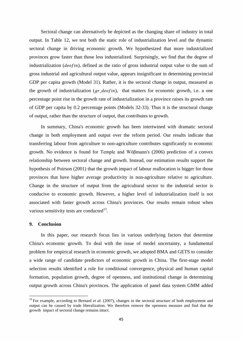
45
Sectoral change can alternatively be depicted as the changing share of industry in total
output. In Table 12, we test both the static role of industrialization level and the dynamic
sectoral change in driving economic growth. We hypothesized that more industrialized
provinces grow faster than those less industrialized. Surprisingly, we find that the degree of
industrialization ( ), defined as the ratio of gross industrial output value to the sum of
gross industrial and agricultural output value, appears insignificant in determining provincial
GDP per capita growth (Model 31). Rather, it is the sectoral change in output, measured as
the growth of industrialization ( ), that matters for economic growth, i.e. a one
percentage point rise in the growth rate of industrialization in a province raises its growth rate
of GDP per capita by 0.2 percentage points (Models 32-33). Thus it is the structural change
of output, rather than the structure of output, that contributes to growth.
In summary, China's economic growth has been intertwined with dramatic sectoral
change in both employment and output over the reform period. Our results indicate that
transferring labour from agriculture to non-agriculture contributes significantly to economic
growth. No evidence is found for Temple and Wöβmann's (2006) prediction of a convex
relationship between sectoral change and growth. Instead, our estimation results support the
hypothesis of Poirson (2001) that the growth impact of labour reallocation is bigger for those
provinces that have higher average productivity in non-agriculture relative to agriculture.
Change in the structure of output from the agricultural sector to the industrial sector is
conducive to economic growth. However, a higher level of industrialization itself is not
associated with faster growth across China's provinces. Our results remain robust when
various sensitivity tests are conducted13
.
9. Conclusion
In this paper, our research focus lies in various underlying factors that determine
China's economic growth. To deal with the issue of model uncertainty, a fundamental
problem for empirical research in economic growth, we adopted BMA and GETS to consider
a wide range of candidate predictors of economic growth in China. The first-stage model
selection results identified a role for conditional convergence, physical and human capital
formation, population growth, degree of openness, and institutional change in determining
output growth across China's provinces. The application of panel data system GMM added
13 For example, according to Bernard et al. (2007), changes in the sectoral structure of both employment and
output can be caused by trade liberalization. We therefore remove the openness measure and find that the
growth impact of sectoral change remains intact.

46
sectoral change to the list. Using that framework, we proceeded to investigate the growth
impact of variables that do not enter formal growth models based on production functions,
i.e. openness, institutional change and sectoral change in some detail14
. Each of them can be
regarded as a form of structural change in the economy, i.e. the relative expansion of the
trade sector, of the private sector, and of the non-agricultural sector.
What light has the analysis thrown on the question posed in our title: why has China
grown so fast? The structure of the economy itself -- level rather than change -- affects the
growth rate in the cases of trade and ownership but not of production. Having a large trade
sector or a large private sector itself raises a province's growth rate. However, change in
structure is even more important. China as a whole has undergone three drastic forms of
structural change over the period of economic reform and each of these structural changes
helps to explain the remarkably high growth rate.
The change of the trade share in GDP has had a positive effect, and not only exports but
also imports have contributed. Posing the counterfactual 'How would the growth rate have
altered if the trade ratio had remained constant?', we find (on the basis of Table 6, Model 4)
that the predicted annual average provincial growth of GDP per capita in China over the
study period was 8.1 percent, whereas the growth of the ratio of trade to GDP was 18.1
percent per annum. The contribution to growth of this structural change was no less than 3.2
percentage points per annum. These results are consistent with growth benefiting from the
improved resource allocation, technology and competition that openness can bring.
The second contribution has come from the rapid privatization of the economy.
Whether we use investment, output or employment as the criterion, we find the effect of state
ownership on growth to be negative and that of private ownership to be positive. Private
enterprise output averaged 22.0 percent of total industrial output in China over the full period.
If it had remained at its 1978 level (1.2 percent), growth would have been 0.7 percentage
points lower, at 7.4 percent per annum (on the basis of Table 8, Model 18). This pattern is
consistent with the improvement in incentives that a greater role for profit-seeking can bring.
Thirdly, it is clear that the remarkable sectoral changes have also made an important
contribution to growth. The average change in the share of employment in the non-
agricultural sector over the full sample period was 1.0 percent per annum. If instead it had not
14 In addition, although sectoral change commonly figures in growth accounting exercises, neither openness nor
institutions are accommodated in the growth accounting approach.

47
occurred, the coefficient (in Table 10, Model 23) implies that China's growth of GDP per
capita would have fallen by one percentage point, from 8.1 to 7.1 percent per annum, holding
other variables constant. This evidence is consistent with there being efficiency gains from
improved sectoral labour allocation and also externalities specific to industry.
By altering mean values of key variables based on model estimation, these simple
simulations contain the questionable assumption that a change in one variable would not
change the other variables in the equation. It is likely that the three types of structural change
are closely interrelated with each other. We therefore estimate an equation that
simultaneously incorporates trade openness, private share of industrial output, and sectoral
change. The full effect of structural change on growth is summed up to 4.1 percent per
annum15
. There remains the possibility that these structural change variables are correlated
with other variables in the regression, for instance, physical and human capital formation, so
that even their joint effect cannot be isolated. We thus use these figures simply to illustrate
the rough orders of magnitude of the potential contribution of structural change to the growth
rate.
Each of these three forms of structural change has involved an improvement in the
efficiency of the economy by bringing it closer to its production frontier. They have also
involved some outward movement of the production frontier, for instance, improvement in
technology from trade openness or from greater incentives for research and development.
However, the main extension of the production possibility curve has come from the
accumulation of physical and human capital -- an issue examined, within the same model
framework, in our companion paper (Ding and Knight, 2008b).
15 The coefficients of all three structural change variables are significantly positive and the contributions of trade
openness, privatization and sectoral change to annual growth rate of GDP per capita are 1.9 percent, 1.3 percent,
and 0.9 percent respectively.
48
References
Abramovitz, M. (1986). Catching Up, Forging Ahead, and Falling Behind. Journal of
Economic History , 46 (2), 385-406.
Acemoglu, D., Johnson, S. and J. A. Robinson. (2001). The Colonial Origins of Comparative
Development: An Empirical Investigation. American Economic Review , 91 (5), 1369-1401.
Acemoglu, D., Johnson, S. and J. A. Robinson. (2005). Institutions as a Fundamental Cause
of Long-Run Growth. In P. Aghion, & S. N. Durlauf, Handbook of Economic Growth (Vol.
1A, pp. 386-472). Amsterdam, The Netherlands: Elsevier B.V.
Alesina, A., Spolaore E., and R. Wacziarg. (2005). Trade, Growth and the Size of Countries.
In P. Aghion, & S. N. Durlauf, Handbook of Economic Growth (Vol. 1B, pp. 1499-1542).
Allen, F., Qian, J. and M. Qian. (2005). Law, Finance, and Economic Growth in China.
Journal of Financial Economics , 77, 57-116.
Anderson, J. E. and J. P. Neary. (1992). Trade Reform with Quotas, Partial Rent Retention,
and Tariffs. Econometrica , 60, 57-76.
Arellano, M. and O. Bover. (1995). Another Look at the Instrumental Variable Estimation of
Error-Components Models. Journal of Econometrics , 68, 29-52.
Arellano, M. and S. Bond. (1991). Some Tests of Specification for Panel Data: Monte Carlo
Evidence and An Application to Employment Equations. Review of Economic Studies , 58,
277-97.
Aron, J. (2000). Growth and Institutions: A Review of the Evidence. The World Bank
Research Observer , 15 (1), 99-135.
Baldwin, R. E. (2003). Openness and Growth: What's the Empirical Relationship. NBER
Working Paper Series No. 9578 .
Bao, S. M., Chang, G. H., Sachs, J. D. and W. T. Woo. (2002). Geographic Factors and
China's Regional Development under Market Reforms, 1978-1998. China Economic Review ,
13, 89-111.
Barro, R. J. (1991). Economic Growth in a Cross Section of Countries. The Quarterly
Journal of Economics , 106 (2), 407-43.
Barro, R. J. and X. Sala-i-Martin. (2004). Economic Growth (second ed.). Cambridge, MA:
The MIT Press.
Beenstock, M. and D. Felsenstein. (2008). Regional Heterogeneity, Conditional Convergence
and Regional Inequality. Regional Studies, 42(4), 475-88.

49
Benhabib, J. and M. M. Spiegel. (1994). The Role of Human Capital in Economic
Development: Evidence from Aggregate Cross-Country Data. Journal of Monetary
Economics , 34 (2), 143-73.
Bernard, A. B., Jensen, B., Redding, S. J. and P. K. Schott . (2007). Firms in International
Trade. Journal of Economic Perspectives , 21 (3), 105-130.
Biggeri, M. (2003). Key Factors of Recent Provincial Economic Growth. Journal of Chinese
Economic and Business Studies , 1 (2), 159-183.
Blomström, M., Lipsey, R. and M. Zejan. (1996). Is Fixed Investment the Key to Economic
Growth? The Quarterly Journal of Economics , 111 (1), 269-76.
Blundell, R. and S. Bond. (1998). Initial Conditions and Moment Restrictions in Dynamic
Panel Data Models. Journal of Econometrics , 87 (1), 115-43.
Bond, S., Hoeffler, A. and J. Temple. (2001). GMM Estimation of Empirical Growth Models.
CEPR discussion paper no. 3048 .
Bond, S., Leblebicioglu, A. and F. Schiantarelli. (2007). Capital Accumulation and Growth:
A New Look at the Empirical Evidence. University of Oxford Working Paper.
Bond, S. and A. Malik. (2007). Explaining Cross-Country Variation in Investment: The Role
of Endowments, Institutions, and Finance. University of Oxford Working Paper.
Bowsher, C. G. (2002). On Testing Overidentifying Restrictions in Dynamic Panel Data
Models. Economics Letters , 77, 211-20.
Bramall, C. (2000). Sources of Chinese Economic Growth 1978-1996. Oxford: Oxford
University Press.
Brandt, L., Hsieh, C. T. and X. D. Zhu. (2008). Growth and Structural Transformation in
China. In L. Brandt, & T. Rawski, China's Great Economic Transformation (pp. 683-728).
New York: Cambridge University Press.
Brandt, L. and X. D. Zhu. (2000). Redistribution in a Decentralized Economy: Growth and
Inflation in China under Reform. Journal of Political Economy , 108 (2), 422-51.
Brun, J. F., Combes, J. L. and M. F. Renard. (2002). Are There Spillover Effects Between
Coastal and Noncoastal Regions in China? China Economic Review , 13, 161-69.
Cai, F., Wang, D. W. and Y. Du. (2002). Regional Disparity and Economic Growth in China:
The Impact of Labour Market Distortions. China Economic Review , 13, 197-212.
Chatfield, C. (1995). Model Uncertainty, Data Mining, and Statistical Inference. Journal of
the Royal Statistical Society , 158, 419-44.
Chen B. Z. and Y. Feng. (2000). Determinants of Economic Growth in China: Private
Enterprise, Education and Openness. China Economic Review , 11, 1-15.

50
Chen, J. and B. M. Fleisher. (1996). Regional Income Inequality and Economic Growth in
China. Journal of Comparative Economics , 22, 141-64.
Commission on Growth and Development. (2008). The Growth Report: Strategies for
Sustained Growth and Inclusive Development (Conference edition).
Corden, W. M. (1974). Trade Policy and Economic Welfare. Oxford: Clarendon Press.
Cull, R. and L. C. Xu. (2005). Institutions, Ownership, and Finance: The Determinants of
Profit Reinvestment among Chinese Firms. Journal of Financial Economics , 77 (1), 117-
146.
Démurger, S. (2001). Infrastructure Development and Economic Growth: An Explanation for
Regional Disparities in China. Journal of Comparative Economics , 29, 95-117.
Denison, E. F. (1967). Why Growth Rates Differ: Postwar Experience in Nine Western
Countries. Washington: Brookings.
Denison, E. F. (1974). Accounting for United States Economic Growth 1929-1969.
Washington: Brookings.
Ding, S. and J. Knight. (2008a). Can the Augmented Solow Model Explain China's Economic
Growth? A Cross-Country Panel Data Analysis. Department of Economics Discussion Paper
No. 380, University of Oxford.
Ding, S. and J. Knight. (2008b). Why has China Grown so Fast? The Role of Physical and
Human Capital Formation.
Dollar, D. (1992). Outward-Oriented Developing Economies Really Do Grow More Rapidly:
Evidence from 95 LDCs, 1976-1985. Economic Development and Cultural Change , 40, 523-
544.
Dollar, D. and A. Kraay. (2004). Trade, Growth, and Poverty. Economic Journal , 114, F22-
F49.
Doornik, J. A. and D. F. Hendry. (2007). Pcgive 12 Voume I: Empirical Econometric
Modelling. London: Timberlake Consultants Press.
Dowrick, S. and N. Gemmell. (1991). Industrialization, Catching Up and Economic Growth:
A Comparative Study Across the World's Capitalist Economies. Economic Journal , 101
(405), 263-275.
Easterly, W. and R. Levine. (2001). What Have We Learned from a Decade of Empirical
Research on Growth? It's not Factor Accumulation: Stylized Facts and Growth Models.
World Bank Economic Review , 15, 177-219.
Edwards, S. (1993). Openness, Trade Liberalization, and Growth in Developing Countries.
Journal of Economic Literature , 31, 1358-1393.

51
Edwards, S. (1998). Openness, Productivity, and Growth: What Do We Really Know?
Economic Journal , 108 (2), 383-398.
Feder, G. (1986). Growth in Semi-Industrial Countries: A Statistical Analysis. In H. Chenery,
S. Robinson, & M. Syrquin, Industrialization and Growth: A Comparative Study (pp. 263-
282). Washington, D. C.: Oxford University Press.
Fernández, C., Ley, E. and M. F. J. Steel. (2001). Model Uncertainty in Cross-Country
Growth Regressions. Journal of Applied Econometrics , 16 (5), 563-76.
Frankel, J. A. and D. Romer. (1999). Does Trade Cause Growth? American Economic Review
, 89 (3), 379-399.
Garnaut, R., Song, L., Tenev, S. and Y. Yao. (2005). China's Ownership Transformation:
Processes, Outcomes, Prospects. Washington, DC: World Bank.
Grossman, G. and E. Helpman. (1995). Innovatoin and Growth in the Global Economy.
Cambridge, MA: MIT Press.
Guariglia, A. and S. Poncet. (2006). Could Financial Distortions be No Impediment to
Economic Growth After All? Evidence from China. The University of Nottingham China and
the World Economy Research Paper Series No. 36 .
Guariglia, A., Liu, X. and L. Song. (2008). Is the Growth of Chinese Firms Constrained by
Internal Finance? Mimeograph, University of Nottingham .
Hall, R. E. and C. I. Jones. (1997). Levels of Economic Activity Across Countries. American
Economic Review , 87 (2), 173-177.
Hall, R. E. and C. Jones. (1999). Why Do Some Countries Produce So Much More Output
Per Worker Than Others? . Quarterly Journal of Economics , 114 (1), 83-116.
Hao, C. (2006). Development of Financial Intermediation and Economic Growth: The
Chinese Experience. China Economic Review , 17, 347-62.
Harrison, A. (1996). Openness and Growth: A Time Series, Cross-Country Analysis for
Developing Countries. Journal of Development Economics , 48, 419-417.
Hasan, I., Wachtel, P. and M. M. Zhou. (2008). Institutional Development, Financial
Deepening and Economic Growth: Evidence from China. Journal of Banking and Finance .
Hendry, D. F. and H. M. Krolzig. (2004). We Ran One Regression. Oxford Bulletin of
Economics and Statistics , 66 (5), 799-810.
Holz, C. A. (2006). China's Reform Period Economic Growth: How Reliable are Augus
Maddison's Estimates? Review of Income and Wealth, 52 (1), 85-119.
Hoover, K. D. and S. J. Perez. (2004). Truth and Robustness in Cross-Country Growth
Regressions. Oxford Bulletin of Economics and Statistics , 66 (5), 765-98.

52
Huang, Y. F. (2005). What Determines Financial Development. Department of Economics
Discussion Paper No. 05/580, University of Bristol .
Islam, N. (1995). Growth Empirics: A Panel Data Approach. The Quarterly Journal of
Economics , 110 (4), 1127-70.
Jefferson, G. H., Mai, L. and J. Zhao. (1998). Reforming Property Rights in China's Industry.
In G. H. Jefferson, & I. Singh, Enterprise Reform in China (pp. 107-125). New York: Oxford
University Press.
Jones, D. C., Li, C. and A. L. Owen. (2003). Growth and Regional Inequality in China during
the Reform Era. China Economic Review , 14, 186-200.
Kaldor, N. (1967). Strategic Factors in Economic Development. Ithaca: Cornell University.
Keidel, A. (2007). China's Looming Crisis--Inflation Returns. Carnegie Endowment for
International Peace Policy Brief , 54.
Knack, S. and P. Keefer . (1995). Institutions and Economic Performance: Cross-Country
Tests Using Alternative Institutional Measures. Economics and Politics , 7 (3), 207-227.
Knight, J. and S. Li. (1999). Fiscal Decentralization: Incentives, Redistribution and Reform in
China. Oxford Development Studies , 27 (1), 5-32.
Knight, J. and L. Song. (2005). Towards a Labour Market in China. Oxford: Oxford
University Press.
Knight, J., Li, S. and Q. Deng. (2008). Education and the Poverty Trap in Rural China.
University of Oxford Centre for the Study of African Economics Working Paper Series No.
2008-02.
Knight, J. and L. Song. (2008). China's Emerging Urban Wage Structure, 1995-2002. In B.
Gustafsson, S. Li, & T. Sicular, Inequality and Public Policy in China (pp. 221-242).
Cambridge: Cambridge University Press.
Kraay, A. (1999). Exports and Economic Performance: Evidence from a Panel of Chinese
Enterprises. Revue d'Economie Du Developpement , 1 (2), 183-207.
Kuijs, L. (2005). Investment and Saving in China. World Bank Policy Research Working
Paper No. 3633.
Lardy, R. N. (2002). China will Keep on Growing. The Wall Street Journal Asia , 14.
Lawrence, R. Z. (1996). Single World, Divided Nations? Paris: OECD.
Leamer, E. E. (1978). Specification Searches. New York: John Wiley & Sons.
Leamer, E. E. (1983). Let's Take the Con Out of Econometrics. American Economic Review ,
73 (1), 31-43.

53
Leamer, E. E. (1985). Sensitivity Analysis Would Help. American Economic Review , 75 (3),
308-13.
Leamer, E. E. (1988). Measures of Openness. In R. E. Baldwin, Trade Policy Issues and
Empirical Analysis (pp. 147-204). Chicago: The University of Chicago Press.
Levine, R. and D. Renelt. (1992). A Sensitivity Analysis of Cross-Country Growth
Regressions. American Economic Review , 82 (4), 942-63.
Lewis, W. A. (1954). Economic Development with Unlimited Supplies of Labour.
Manchester School of Economic and Social Studies , 22, 139-191.
Li, H., Liu, Z. N. and I. Rebelo. (1998). Testing the Neoclassical Theory of Economic
Growth: Evidence from Chinese Provinces. Economics of Planning , 31, 117-32.
Lin, Y. F. (1992). Rural Reforms and Agricultural Growth in China. American Economic
Review , 82 (1), 34-51.
Lin, Y. F. and J. B. Nugent. (1995). Institutions and Economic Development. In J. Behrman,
& T. N. Srinivasan, Handbook of Development Economics (Vol. IIIA, pp. 2303-2370).
Amsterdam, The Netherlands: Elsevier Science B.V.
Lin, Y. F. and T. Zhu. (2001). Ownership Restructuring in Chinese State Industry: An
Analysis of Evidence on Initial Organizaional Changes. The China Quarterly , 166, 298-334.
Lin, Y. F. (2007). Development and Transition: Idea, Strategy, and Viability. Marshall
Lecture. Cambridge University.
Liu, X., Burridge, P. and P. J. N. Sinclair. (2002). Relationships between Economic Growth,
Foreign Direct Investment and Trade: Evidence from China. Applied Economics , 34 (11),
1433-1440.
Lucas, R. E. (1988). On the Mechanics of Economic Development. Journal of Monetary
Economics , 22, 3-42.
Lucas, R. E. (2002). Lectures on Economic Growth. MA: Harvard University Press.
Maddison, A. 1998. Chinese Economic Performance in the Long Run. Paris: OECD.
Malik, A. and J. R. W. Temple. (2005). The Geography of Output Volatility. CSAE Working
Paper No. 2005-07, University of Oxford .
Mankiw, N. G., Romer, D. and D. N. Weil. (1992). A Contribution to the Empirics of
Economic Growth. The Quarterly Journal of Economics , 107 (2), 407-37.
Mauro, P. (1995). Corruption and Growth. Quarterly Journal of Economics , 110 (3), 681-
712.
Modigliani, F. and S. L. Cao. (2004). The Chinese Saving Puzzle and the Life-Cycle
Hypothesis. Journal of Economic Literature, 42(1), 145-170.

54
Naughton, B. (2006). The Chinese Economy: Transitions and Growth. Cambridge, MA: The
MIT Press.
Nickell, S. (1981). Biases in Dynamic Models with Fixed Effects. Econometrica , 49 (6),
1417-1426.
North, D. (1990). Institutions, Institutional Change, and Economic Performance. New York:
Cambridge University Press.
Nye, H. L. M., Reddy, S. G. and K. Watkins. (2002). Dollar and Kraay on 'Trade, Growth,
and Poverty': A Critique. Unpublished manuscript .
Owen, P. D. (2003). General-to-Specific Modelling Using Pcgets. Journal of Economic
Surveys , 17 (4), 609-27.
Park, A., Yang, D., Shi, X. Z. and Y. Jiang. (2008). Exporting and Firm Performance:
Chinese Exporters and the Asian Financial Crisis. Conference on 'Confronting the Challenge
of Technology for Development: Experiences from the BRICS', University of Oxford .
Poirson, H. (2001). The Impact of Intersectoral Labour Reallocation on Economic Growth.
Journal of African Economies , 10 (1), 37-63.
Pritchett, L. (1996). Measuring Outward Orientation in Developing Countries: Can it Be
Done? Journal of Development Economics , 49 (2), 307-335.
Pritchett, L. (1999). Where Has All the Education Gone? The World Bank Economic Review ,
15 (3), 367-91.
Raftery, A. E. (1995). Bayesian Model Selection in Social Research. In P. V. Marsden,
Sociological Methodology. Cambridge: Blackwells.
Raiser, M. (1998). Subsidising Inequality: Economic Reforms, Fiscal Transfers and
Convergence Across Chinese Provinces. The Journal of Development Studies , 34 (3), 1-26.
Ravallion, M. and S. H. Chen. (2007). China’s (Uneven) Progress Against Poverty. Journal
of Development Economics , 82, 1-42.
Rawski, T. (2001). What is Happening to China's GDP Statistics? China Economic Review
12, 347-354.
Riedel, J., Jin, J. and J. Gao. (2007). How China Grows: Investment, Finance and Reform.
Princeton: Princeton University Press.
Robinson, S. (1971). Sources of Growth in Less Developed Countries: A Cross-Section
Study. Quarterly Journal of Economics , 85 (3), 391-408.
Rodríguez, F. and D. Rodrik. (2001). Trade Policy and Economic Growth: A Skeptic's Guide
to the Cross-National Evidence. In B. a. Bernanke, Macroeconomics Annual 2000 (pp. 261-
324). Cambridge: MIT Press for NBER.

55
Rodrik, D. (1999). The New Global Economy and Developing Countries: Making Openness
Work. Washington, DC: Johns Hopkins University Press for the Overseas Development
Council.
Rodrik, D. (2003). Introduction: What Do We Learn from Country Narratives? In D. Rodrik,
In Search of Prosperity: Analytic Narratives on Economic Growth (pp. 1-19). Princeton and
Oxford: Princeton University Press.
Romer, P. M. (1990). Are Nonconvexities Important for Understanding Growth? American
Economic Review, 80(2), 97-103.
Sachs, J. D. and A. M. Warner. (1995). Economic Reform and the Process of Economic
Integration. Brookings Papers of Economic Activity , 1-118.
Sala-i-Martin, X. X. (1997). I Just Ran Two Million Regressions. American Economic
Review , 87 (2), 178-83.
Sala-i-Martin, X., Doppelhofer, G. and R. Miller. (2004). Determinants of Long-Run Growth:
A Bayesian Averaging of Classical Estimates (BACE) Approach. American Economic
Review , 94 (4), 813-35.
Schwarz, G. (1978). Estimating the Dimension of a Model. Annals of Statistics , 6, 461-64.
Scott, M. F. (1989). A New View of Economic Growth. Oxford: Clarendon Press.
Scott, M. F. (1993). Explaining Economic Growth. American Economic Review, Papers and
Proceedings of the Hundred and Fifth Annual Meeting of the American Economic
Association , 83 (2), 421-25 .
Smyth, R. (1998). Property Rights in China's Economic Reforms. Communist and Post-
Communist Studies , 31 (3), 235-248.
Solow, R. M. (1956). A Contribution to the Theory of Economic Growth. Quarterly Journal
of Economics , 70, 65-94.
Taylor, J. R. (1988). Rural Employment Trends and the Legacy of Surplus Labour. China
Quarterly , 116, 736-766.
Temple, J. (1999). The New Growth Evidence. Journal of Economic Literature , 37 (1), 112-
56.
Temple, J. and L. Wöβmann. (2006). Dualism and Cross-Country Growth Regressions.
Journal of Economic Growth , 11, 187-228.
Vollrath, D. (2005). How Important are Dual Economy Effects for Aggregate Productivity?
Manuscript, University of Houston .
Wacziarg, R. (2001). Measuring the Dynamic Gains from Trade. World Bank Economic
Review , 15 (3), 393-429.
56
Wei, S. J. (1995). Open Door Policy and China's Rapid Growth: Evidence from City-Level
Data. In T. Ito, & A. Krueger, Growth Theories in Light of the East Asian Experience.
University of Chicago Press.
Windmeijer, F. (2005). A Finite Sample Correction for the Variance of Linear Efficient Two-
Step GMM Estimators. Journal of Econometrics , 126, 25-51.
Winters, L. A. (2004). Trade Liberalisation and Economic Performance: An Overview.
Economic Journal , 114, F4-F21.
Yanikkaya, H. (2003). Trade Openness and Economic Growth: A Cross-Country Empirical
Investigation. Journal of Development Economics , 72, 57-89.
Yao, S. (2006). On Economic Growth, FDI and Exports in China. Applied Economics , 38,
339-51.
Ying, L. G. (2003). Understanding China's Recent Growth Experience: A Spatial
Econometric Perspective. The Annals of Regional Science , 37, 613-628.
Young, A. (2003). Gold into Base Metal: Productivity Growth in the People's Republic of
China during the Reform Period. Journal of Political Economy, 111 (6), 1220-1261.
Zhang, W. (2001). Rethinking Regional Disparity in China. Economics of Planning , 34, 113-
38.

57
Appendix 1 : Model Selection Procedures
Bayesian model averaging (BMA)
The following brief discussion of the theory behind BMA draws heavily on Raftery (1995),
Sala-i-Martin et al. (2004), Malik and Temple (2005) and Huang (2005).
A natural way to think about model uncertainty is to admit that we do not know which model
is 'true' and instead, attach probabilities to different possible models. BMA treats parameters
and models as random variables and summarizes the uncertainty about the model in terms of
a probability distribution over the space of all possible models.
Suppose we want to make inference about an unknown quantity of interest (such as a
parameter), , given data . There are a large number of possible statistical models,
for the data space. If we consider only linear regression models but are unsure
about which possible regressors to include, there could be as many as models
considered. Bayes' rule and basic probability theory suggest that the posterior distribution of
the parameters is the weighted average of all the possible conditional posterior densities with
the weights given by the posterior probabilities of each of the possible models. Then the
posterior distribution of given data is
, (A.1)
where is the posterior distribution of given the model , and
is the posterior model probability. Thus the BMA posterior distribution of is a weighted
average of the posterior distributions of under each of the models, weighted by their
posterior model probabilities.
Based on Bayes' theorem, the posterior model probability is given by
, (A.2)
where is the prior probability of model , and is the integrated
likelihood of model , obtained by integrating over the unknown parameters
, (A.3)
where is the parameter of model , is the likelihood of under model
, and is the prior distribution over the parameter space associated with
model . The integrated likelihood is a high dimensional integral that can be
hard to calculate analytically, and therefore some simplification and approximations are
required. Raftery (1995) proposes that a convenient solution is to approximate twice the log
Bayes factor using the Bayesian Information Criterion ( ) due to Schwarz (1978). One
important advantage of the approximation is that it avoids the need for an explicit
specification for the prior distributions . To represent no prior preference for any
model, each model presumed equally likely before examining the data, i.e. all possible

58
models have equal prior probabilities or . Then the posterior model probability
can be calculated as
. (A.4)
Then we are ready to implement a systematic form of inference for different parameters of
interest, which is superior to the ad hoc strategies often used in cross-province growth study
on China. One potential difficulty in implementing BMA is the sheer range of possible
models. To deal with this problem, Occam's Window technique and Markov Chain Monte
Carlo techniques can be adopted. The former focuses on a subset defined by Occam's
Window technique and treats all the worst-fitting models outside the subset as having zero
posterior probability. Embodying the principle of parsimony, this method considerably
reduces the number of possible models, and in the meantime encompasses the inherent model
uncertainty present. The latter has the advantage of simultaneously selecting variables and
identifying outliers, but requires a larger sample size relative to the regressor set. Given our
small sample size (N=30), we use the package bicreg for S-Plus or R written by Adrian
Raftery, where the computational procedure for Occam's Window technique is implemented
to exclude the relatively unlikely models.
General-to-specific approach (GETS)
The following brief discussion of general-to-specific methodology draws heavily on Owen
(2003), Hendry and Krolzig (2004), Hoover and Perez (2004), and Doornik and Hendry
(2007).
The general-to-specific model selection is also referred to as the LSE approach to
econometric modelling. It begins with the idea that the truth can be characterized by a
sufficiently rich regression (the general regression), i.e. if every possible variable is included
in the regression, then the general regression must contain all the information about the true
determinants. However, the model may not be in a perspicacious form, therefore the
information content can be sharpened by a more parsimonious regression (the specific
regression). The specific regression is a valid restriction of the general model if it is
statistically well specified and it encompasses every other parsimonious regression.
The specification of the general unrestricted model (GUM) from which reductions commence
is crucial to the performance of GETS approach, i.e. the specific model will not be able to
improve on a bad GUM. Economic theory and previous empirical findings can play a central
role in providing 'prior simplification'. Once a GUM is specified, insignificant variables are
eliminated to reduce complexity, and diagnostic checks (normality test, heteroscedasticity
test, F test for parameter constancy and Reset test for function form) on the validity of these
reductions ensures congruence of the final model. In order to keep all promising variables in
the final model, we set the target size as huge (level of significance: 0.1).
The computing software we use to implement GETS modelling is Autometrics (part of Pcgive
12 in OxMetrics 5, which was recently released in late 2007). It is an upgraded version of

59
Pcgets, taking many features of the earlier implementations, but also differing in several
important aspects. For example, Autometrics relied much less on presearch as the simulation
experiments show almost the same operating characteristics with and without presearch;
Autometrics does not implement the multiple-path search (which is an unstructured way of
searching the model space), instead, it considers the whole search space from the outset using
a tree search, discarding parts in a systematic way; while using roughly the same battery of
diagnostic tests, Autometrics postpones the testing until a candidate terminal model has been
found, and if necessary, backtracking is used to find a valid model, making the
implementation faster and resulting in more parsimonious models; and a block-search
algorithm is used by Autometrics to handle the case of more variables than observations. In
brief, simulation results show that Autometrics is similar with Pcgets in terms of power, but
had better size performance in some cases.
Appendix 2 : Temple and Wöβmann (2006)'s model
This part draws heavily on Temple and Wöβmann (2006) and Ding and Knight (2008a).
Temple and Wöβmann (2006) developed an empirical model to examine the impact of labour
reallocation on aggregate productivity growth and they augmented the conventional growth
regressions based on the MRW framework so as to allow for sectoral change. Their basic idea
is that changes in the structure of employment will raise aggregate productivity when the
marginal product of labour varies across sectors. If the marginal product of labour is lower in
agriculture, then the movement of agricultural workers to sectors where the marginal product
is higher will raise total output. Since this additional output is produced without change in
the total input of capital and labour, the reallocation of labour raises aggregate productivity.
It is a general equilibrium model of production with two sectors (a rural agricultural and an
urban non-agricultural sector) and two factors (capital and labour). Total output is given by
, (A.5)
where is the relative price of the urban sector good; and are output quantities in
agriculture and non-agriculture; and is a GDP price deflator. The production function
in each sector has constant returns to scale and is given by
, (A.6)
, (A.7)
where and are TFP in agriculture and non-agriculture respectively. Assuming that
workers are paid their marginal products gives
, (A.8)
, (A.9)

60
where and are wages in agriculture and non-agriculture respectively; and the
subscript denotes the partial derivative with respect to labour. Capital also receives its
marginal product in both sectors, i.e. , where is the rental rate on
capital and the subscript is the partial derivative with respect to capital. This model
assumes that any observed effects of reallocation arise because of marginal product
differentials and that the propensity to migrate depends on the ratio of wages in the two
sectors. Migration will cease when the intersectoral wage ratio falls to a level denoted by ,
so the long-run migration equilibrium is
, (A.10)
where . The relationship between the extent of sectoral change and wage ratio can be
expressed as
, (A.11)
where is the migration propensity, defined by , where is the share of
agricultural employment in total employment; and is the speed of adjustment to the long-
run equilibrium. The 'odds ratio' for migration is increasing in the wage gap between the two
sectors. Rearranging (A.11) gives
, (A.12)
so the extent of current wage ratio can be deduced using information on the observed pace of
sectoral change. In this model, the wage differential varies across countries according to the
value of . By assuming that the speed of adjustment ( ), the equilibrium differential ( )
and the labour share in total output ( ) are constant across economies, Temple and
Wöβmann (2006) derived the following expression for the aggregate Solow residual
, (A.13)
where is the nominal output share for agriculture at time t, or ; is the
labour share in total output, or ; and is the share of non-agricultural employment
in total employment, or .
In the presence of an intersectoral wage differential, the aggregate Solow residual can thus be
decomposed as a weighted average of the sectoral TFP growth rates plus the 'growth bonus'
obtained by reallocating labour to a sector where its marginal product is higher. Since the
migration propensity is related to the extent of sectoral change as measured by , equation
(A.13) implies a convex relationship between growth and sectoral change. The intuition is
that the growth impact of a given extent of sectoral change will be greatest in those countries
experiencing more rapid sectoral change, as these are also the countries in which the
intersectoral wage differential is greatest. Note that the two sectoral change terms in equation
(A.13) will disappear when there is no wage differential in equilibrium, , and the

61
adjustment process in response to disequilibrium is instantaneous, . Since it was not
possible to measure capital stocks at the sectoral level, Temple and Wöβmann (2006) treated
sectoral TFP as unobservable and relied on a vector to capture the cross-section variation in
aggregate TFP growth that is not due to sectoral change, as follows
, (A.14)
where is a vector of determinants of aggregate TFP growth including initial level of
aggregate TFP and regional differences in technology and institutions proxied by regional
dummies; and the sectoral change terms are defined as
(A.15)
. (A.16)
Temple and Wöβmann (2006) then extended MRW's model by including the sectoral change
terms derived above to proxy the varying productivity growth across countries. Given the
Cobb-Douglas production function ), TFP growth is equal to the
growth rate of efficiency ( ) times the exponent on the efficiency index ( ). In the
presence of wage differentials, TFP growth is a function of sectoral change terms as shown in
equation (A.14). Then the extension of MRW's model takes the form
, (A.17)
where is a vector of explanatory variables including rates of saving, physical and human
capital accumulation. Thus, the specification of equation (A.17) is a hybrid of the Solow
model with an aggregate production function and a two-sector framework with sectoral
product differentials.
Despite its approximations and limits, this model has a number of comparative advantages.
Firstly, compared with the conventional MRW models, equation (A.17) allows for cross-
country variation in productivity growth by taking into account the effect of labour
reallocation between sectors with different productivity. Secondly, unlike the use of
accounting methods to measure TFP growth, this model does not involve the task of
measuring the capital stock, which might be problematic for developing countries.
When replacing the assumption that the labour share in output, , is the same across
countries by an assumption that all countries have the same Cobb-Douglas technologies in
agriculture, Temple and Wöβmann (2006) constructed a second set of sectoral change terms
(A.18)
, (A.19)
where is the share of agriculture in total value added. This alternative set of sectoral change
terms adds , i.e. the share of agriculture in value added divided by the share of employment.
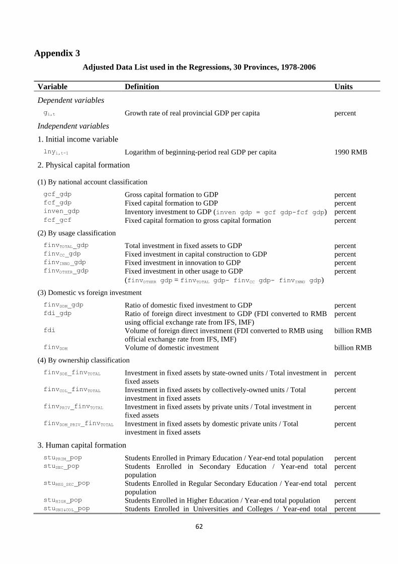
62
Appendix 3
Adjusted Data List used in the Regressions, 30 Provinces, 1978-2006
Variable Definition Units
Dependent variables
gi,t Growth rate of real provincial GDP per capita percent
Independent variables
1. Initial income variable
lnyi,t-1 Logarithm of beginning-period real GDP per capita 1990 RMB
2. Physical capital formation
(1) By national account classification
gcf_gdp Gross capital formation to GDP percent fcf_gdp Fixed capital formation to GDP percent inven_gdp Inventory investment to GDP (inven_gdp = gcf_gdp-fcf_gdp) percent fcf_gcf Fixed capital formation to gross capital formation percent
(2) By usage classification
finvTOTAL_gdp Total investment in fixed assets to GDP percent finvCC_gdp Fixed investment in capital construction to GDP percent finvINNO_gdp Fixed investment in innovation to GDP percent finvOTHER_gdp Fixed investment in other usage to GDP
(finvOTHER_gdp = finvTOTAL_gdp- finvCC_gdp- finvINNO_gdp)
percent
(3) Domestic vs foreign investment
finvDOM_gdp Ratio of domestic fixed investment to GDP percent fdi_gdp Ratio of foreign direct investment to GDP (FDI converted to RMB
using official exchange rate from IFS, IMF)
percent
fdi Volume of foreign direct investment (FDI converted to RMB using
official exchange rate from IFS, IMF)
billion RMB
finvDOM Volume of domestic investment billion RMB
(4) By ownership classification
finvSOE_finvTOTAL Investment in fixed assets by state-owned units / Total investment in
fixed assets
percent
finvCOL_finvTOTAL Investment in fixed assets by collectively-owned units / Total
investment in fixed assets
percent
finvPRIV_finvTOTAL Investment in fixed assets by private units / Total investment in
fixed assets
percent
finvDOM_PRIV_finvTOTAL Investment in fixed assets by domestic private units / Total
investment in fixed assets
percent
3. Human capital formation
stuPRIM_pop Students Enrolled in Primary Education / Year-end total population percent stuSEC_pop Students Enrolled in Secondary Education / Year-end total
population
percent
stuREG_SEC_pop Students Enrolled in Regular Secondary Education / Year-end total
population
percent
stuHIGH_pop Students Enrolled in Higher Education / Year-end total population percent stuUNI&COL_pop Students Enrolled in Universities and Colleges / Year-end total percent
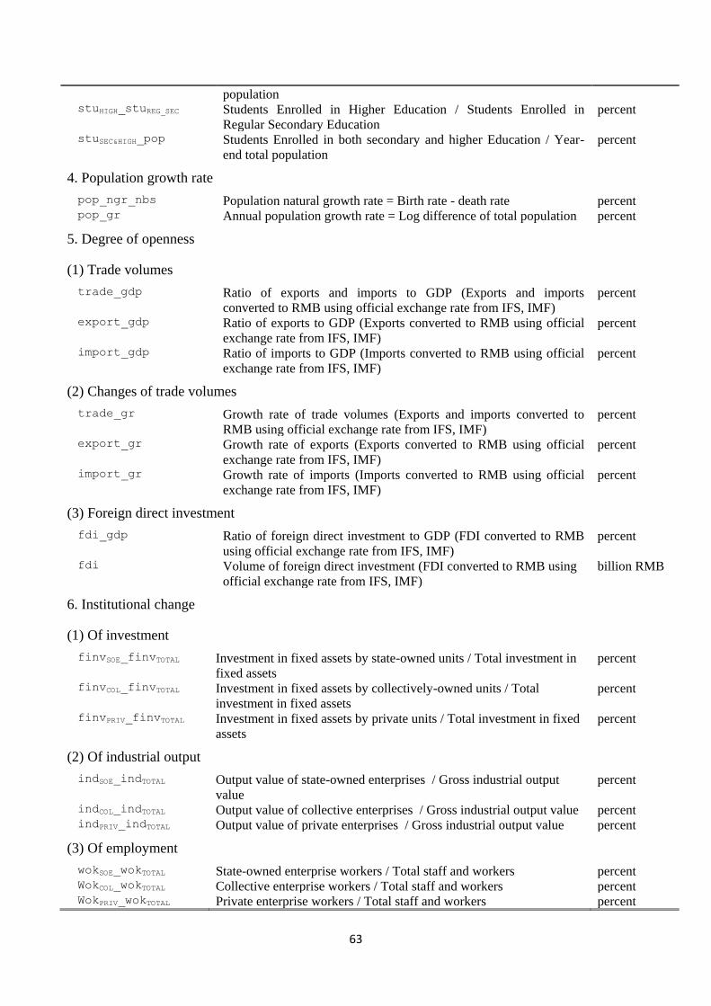
63
population stuHIGH_stuREG_SEC Students Enrolled in Higher Education / Students Enrolled in
Regular Secondary Education
percent
stuSEC&HIGH_pop Students Enrolled in both secondary and higher Education / Year-
end total population
percent
4. Population growth rate
pop_ngr_nbs Population natural growth rate = Birth rate - death rate percent pop_gr Annual population growth rate = Log difference of total population percent
5. Degree of openness
(1) Trade volumes
trade_gdp Ratio of exports and imports to GDP (Exports and imports
converted to RMB using official exchange rate from IFS, IMF)
percent
export_gdp Ratio of exports to GDP (Exports converted to RMB using official
exchange rate from IFS, IMF)
percent
import_gdp Ratio of imports to GDP (Imports converted to RMB using official
exchange rate from IFS, IMF)
percent
(2) Changes of trade volumes
trade_gr Growth rate of trade volumes (Exports and imports converted to
RMB using official exchange rate from IFS, IMF)
percent
export_gr Growth rate of exports (Exports converted to RMB using official
exchange rate from IFS, IMF)
percent
import_gr Growth rate of imports (Imports converted to RMB using official
exchange rate from IFS, IMF)
percent
(3) Foreign direct investment
fdi_gdp Ratio of foreign direct investment to GDP (FDI converted to RMB
using official exchange rate from IFS, IMF)
percent
fdi Volume of foreign direct investment (FDI converted to RMB using
official exchange rate from IFS, IMF)
billion RMB
6. Institutional change
(1) Of investment
finvSOE_finvTOTAL Investment in fixed assets by state-owned units / Total investment in
fixed assets
percent
finvCOL_finvTOTAL Investment in fixed assets by collectively-owned units / Total
investment in fixed assets
percent
finvPRIV_finvTOTAL Investment in fixed assets by private units / Total investment in fixed
assets
percent
(2) Of industrial output
indSOE_indTOTAL Output value of state-owned enterprises / Gross industrial output
value
percent
indCOL_indTOTAL Output value of collective enterprises / Gross industrial output value percent indPRIV_indTOTAL Output value of private enterprises / Gross industrial output value percent
(3) Of employment
wokSOE_wokTOTAL State-owned enterprise workers / Total staff and workers percent WokCOL_wokTOTAL Collective enterprise workers / Total staff and workers percent WokPRIV_wokTOTAL Private enterprise workers / Total staff and workers percent

64
7. Sectoral change
(1) Temple and Wöβmann (2006)'s specification
s Agricultural share of GDP (Primary sector GDP / Total GDP) percent a Agricultural share of employment (Primary sector employment /
Total number of employed persons)
percent
m Non-agricultural share of employment (m=1-a) percent p Migration propensity (p= -4 a/a)
MGROWTH Linear sectoral change term: Change of non-agricultural share of
employment (4m)
percent
DISEQ Non-linear sectoral change term: Change of non-agricultural share
of employment adjusted by migration propensity (p/(1-p)* 4m)
percent
MGROWTH2 Linear sectoral change term: Change of non-agricultural share of
employment * Average labour productivity in agricultural sector (4
m*s/a)
percent
DISEQ2 Non-linear sectoral change term: Change of non-agricultural share
of employment adjusted by migration propensity * Average labour
productivity in agricultural sector (p/(1-p)*4 m*s/a)
percent
(2) Poirson (2001)'s specification
MGROWTH*RLP Change in employment share in non-agricultural sector weighted by
relative labour productivity (RLP = ratio of average labour
productivity in non-agriculture to that in agriculture)
percent
(3) Degree of industrialization
deofin Degree of industrialization (Gross industrial output value / (Gross
industrial output value + Gross agricultural output value)) percent
gr_deofin Growth rate of degree of industrialization (4 deofin) percent
8. Infrastructure
railway_area Mileages of railways per square kilometre (Total railway length /
Area)
percent
highway_area Mileages of highways per square kilometre (Total highways length /
Area)
percent
post&tele_gdp Business volume of post and telecommunication / GDP percent
9. Financial development
loan_gdp Total bank loan outstanding / GDP percent saving_gdp Savings deposit in urban and rural areas / GDP percent
10. Geographic location
dumcoastal A dummy variable which is equal to one for coastal provinces
(Liaoning, Hebei, Tianjin, Shandong, Jiangsu, Shanghai, Zhejiang,
Fujian, Guangdong, and Hainan, plus Beijing), and zero otherwise.
0 or 1
Note: All the variables are calculated in 1990 constant prices and price indices are province-specific.

65
Pre-test data cleaning rules
o Treat any observation of annual growth rate of GDP per capita / per worker above - /
+ 25% as outlier;
o Treat any observation of annual population growth rate above - / + 8% as outlier;
o Treat any observation of annual employment growth rate above - / + 8% as outlier.