chinese-english statistical machine translation by parsing
TRANSCRIPT

Chinese-English Statistical Machine Translation by Parsing
Yue Zhang Mansfield College
Computing Laboratory University of Oxford
2006
I
Abstract
Statistical machine translation (SMT) has evolved from the word-based level to higher levels of abstraction. Currently the best known systems are phrased-based, and recent research has started to explore tree-based systems with syntactical information. This thesis aims to study large-scale Chinese-English SMT using a syntactic tree-based model. From the engineering point of view, SMT systems are very complex to build. However, existing pieces of software can bring the work load to a manageable level for this thesis. Using the GenPar framework and other software, this thesis studies Chinese-English SMT by parsing by large-scale experiments. This is the first application of GenPar on Chinese-English SMT. The experiments show that the accuracy of Chinese-English SMT by parsing is comparable to existing SMT by parsing of other language pairs. However, the accuracy of current MT methods is still largely below human translation, and is influenced by the difference between training and testing data, such as the writing style and domain. Two important factors in the SMT by parsing model are studied, and it is observed that though the accuracy of word-to-word alignment influences the translation accuracy, the mono-lingual English and Chinese grammars do not have a significant impact on the results. From the above observations, advantages and weaknesses of the SMT model are analysed, and possible future improvements for Chinese-English SMT are suggested. This thesis is organised in three main parts. The first chapter presents the introduction and overview of the thesis. The second and third chapters summarise the related theories by literature review, giving a detailed exposition of the theory of SMT and SMT by parsing. The last two chapters report the novel experiments of Chinese-English SMT by generalised parsing. By discussing the experimental output, the last chapter summarises this thesis and proposes further work.

II
Acknowledgements
I would like to express my gratitude to my wonderful supervisor Dr. Stephen Clark, who has been giving me knowledgeable guidance through the work of this thesis, and thoroughly reviewed my draft many times. I am also thankful to my friends, including Xi Cheng, who has been discussing new ideas with me and giving me inspirations since the beginning of the course, Hugh Gibson, who has been listening to my problems, making kind suggestions, and Xuan Wang, who visited me and gave me much strength. Most of all, I want to thank my girlfriend Qian, for sharing my happiness and difficulties all the time (and reading the introduction!), and my parents, for supporting my choice and encouraging me as always.

III
Contents
0HAbstract ............................................................................................................................. 127HI 1HAcknowledgements...................................................................................................... 128HII 2HContents ......................................................................................................................... 129HIII 3HList of Tables.................................................................................................................. 130HV 4HList of Figures............................................................................................................... 131HVI 5HChapter 1 Introduction............................................................................................... 132H1
6H1.1 Introduction .................................................................................................. 133H1 7H1.1.1 Machine translation ............................................................................. 134H1 8H1.1.2 Statistical machine translation ........................................................... 135H1 9H1.1.3 Grammars – the provider of linguistic information ........................ 136H5 10H1.1.4 Synchronous grammars and SMT by parsing.................................. 137H6 11H1.1.5 Chinese-English SMT by parsing...................................................... 138H8
12H1.2 Overview........................................................................................................ 139H9 13H1.3 Contributions ................................................................................................ 140H9
14HChapter 2 Background ............................................................................................. 141H10 15H2.1 The theory of statistical machine translation .................................... 142H10
16H2.1.1 The source-channel model................................................................ 143H10 17H2.1.2 Word-based SMT – the fundamental ideas.................................... 144H11 18H2.1.3 The trend towards higher levels of abstraction.............................. 145H15
19H2.2 The evaluation of machine translation ............................................... 146H17 20H2.2.1 The Bleu metrics ................................................................................ 147H17 21H2.2.2 The NIST metric ................................................................................ 148H19 22H2.2.3 The F-measure .................................................................................... 149H20 23H2.2.4 Summary ............................................................................................. 150H22
24H2.3 The theory of parsing and generalised parsing ............................... 151H22 25H2.3.1 Rule-based parsers ............................................................................. 152H23 26H2.3.2 Statistical parsers................................................................................ 153H26 27H2.3.3 Generalised parsing ........................................................................... 154H31
28HChapter 3 The theory of SMT by parsing ........................................................... 155H33 29H3.1 Statistical GMTG and its generalised parsing .................................. 156H33
30H3.1.1 Generalised multitext grammar (GMTG)....................................... 157H33 31H3.1.2 The statistical model.......................................................................... 158H38 32H3.1.3 Statistical parsing with GMTG ........................................................ 159H40 33H3.1.4 The training process........................................................................... 160H43

IV
34H3.2 Hierarchical alignment by parsing ...................................................... 161H44 35H3.2.1 Calculating combined pseudo production rules from one mono-lingual grammar ............................................................................................. 162H45 36H3.2.2 Calculating combined pseudo production scores from two mono-lingual grammars............................................................................................ 163H47 37H3.2.3 Hierarchical alignment by generalised parsing ............................. 164H47
38H3.3 Translation by bilingual parsing .......................................................... 165H48 39HChapter 4 The details of experiments .................................................................. 166H51
40H4.1 Introduction ................................................................................................ 167H51 41H4.2 Software........................................................................................................ 168H51
42H4.2.1 GenPar – the software framework for generalised parsing ......... 169H51 43H4.2.2 The Bikel statistical (mono-lingual) parser.................................... 170H55 44H4.2.3 The LingPipe libraries for the Chinese segmentation task .......... 171H55 45H4.2.4 The Stanford statistical tagger.......................................................... 172H55 46H4.2.5 GIZA++ – the word alignment tool ................................................ 173H55
47H4.3 Training and testing data ........................................................................ 174H56 48H4.3.1 Training data ....................................................................................... 175H56 49H4.3.2 Testing data......................................................................................... 176H56
50H4.4 Details for a typical experiment ............................................................ 177H57 51H4.4.1 Input for training ................................................................................ 178H57 52H4.4.2 Pre-processing for training ............................................................... 179H58 53H4.4.3 Word alignment.................................................................................. 180H60 54H4.4.4 Hierarchical alignment ...................................................................... 181H62 55H4.4.5 Initialise grammar .............................................................................. 182H63 56H4.4.6 Optimise .............................................................................................. 183H63 57H4.4.7 Input for translation ........................................................................... 184H63 58H4.4.8 Pre-process for translation ................................................................ 185H64 59H4.4.9 Translation .......................................................................................... 186H64 60H4.4.10 Evaluation ........................................................................................... 187H65 61H4.4.11 Summary............................................................................................. 188H65
62H4.5 An overview of all the experiments..................................................... 189H66 63HChapter 5 The results and conclusions ............................................................... 190H67
64H5.1 Test results and discussions ................................................................... 191H67 65H5.1.1 Standard tests ...................................................................................... 192H67 66H5.1.2 The influence of the writing style.................................................... 193H71 67H5.1.3 The role of syntactic information .................................................... 194H73 68H5.1.4 The importance of word-to-word probabilities ............................. 195H75
69H5.2 Summary ...................................................................................................... 196H77 70H5.3 Future work................................................................................................. 197H78
71HReferences...................................................................................................................... 198H80 72HSample code .................................................................................................................. 199H84
73H1. bleu.py – implementing the Bleu metrics (Section 2.2.1).......................... 200H84 74H2. weavefiles.py – the module to weave files together ................................... 201H86
V
List of Tables
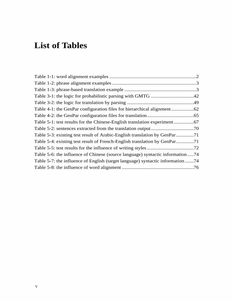
Table 1-1: word alignment examples .....................................................................2 Table 1-2: phrase alignment examples ...................................................................3 Table 1-3: phrase-based translation example .........................................................3 Table 3-1: the logic for probabilistic parsing with GMTG ..................................42 Table 3-2: the logic for translation by parsing .....................................................49 Table 4-1: the GenPar configuration files for hierarchical alignment..................62 Table 4-2: the GenPar configuration files for translation.....................................65 Table 5-1: test results for the Chinese-English translation experiment................67 Table 5-2: sentences extracted from the translation output ..................................70 Table 5-3: existing test result of Arabic-English translation by GenPar ..............71 Table 5-4: existing test result of French-English translation by GenPar..............71 Table 5-5: test results for the influence of writing styles .....................................72 Table 5-6: the influence of Chinese (source language) syntactic information .....74 Table 5-7: the influence of English (target language) syntactic information .......74 Table 5-8: the influence of word alignment .........................................................76
VI
List of Figures
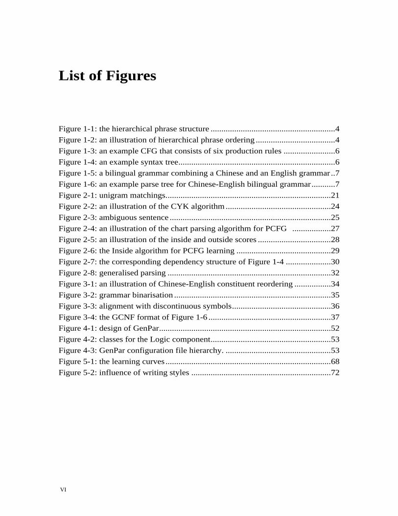
Figure 1-1: the hierarchical phrase structure ..........................................................4 Figure 1-2: an illustration of hierarchical phrase ordering .....................................4 Figure 1-3: an example CFG that consists of six production rules ........................6 Figure 1-4: an example syntax tree.........................................................................6 Figure 1-5: a bilingual grammar combining a Chinese and an English grammar ..7 Figure 1-6: an example parse tree for Chinese-English bilingual grammar...........7 Figure 2-1: unigram matchings.............................................................................21 Figure 2-2: an illustration of the CYK algorithm .................................................24 Figure 2-3: ambiguous sentence ...........................................................................25 Figure 2-4: an illustration of the chart parsing algorithm for PCFG ..................27 Figure 2-5: an illustration of the inside and outside scores ..................................28 Figure 2-6: the Inside algorithm for PCFG learning ............................................29 Figure 2-7: the corresponding dependency structure of Figure 1-4 .....................30 Figure 2-8: generalised parsing ............................................................................32 Figure 3-1: an illustration of Chinese-English constituent reordering .................34 Figure 3-2: grammar binarisation .........................................................................35 Figure 3-3: alignment with discontinuous symbols..............................................36 Figure 3-4: the GCNF format of Figure 1-6 .........................................................37 Figure 4-1: design of GenPar................................................................................52 Figure 4-2: classes for the Logic component........................................................53 Figure 4-3: GenPar configuration file hierarchy. .................................................53 Figure 5-1: the learning curves .............................................................................68 Figure 5-2: influence of writing styles .................................................................72
1
Chapter 1
Introduction
1.1 Introduction 1.1.1 Machine translation The idea of machine translation (MT) can be traced back to the seventeenth century, but it became realistically possible only in the middle of the twentieth century (Hutchins, 2005). Soon after the first computers were developed, research began on MT algorithms. The earliest MT systems consisted primarily of large bilingual dictionaries and sets of translation rules. Dictionaries were used for word level translation, while rules controlled higher level aspects such as word order and sentence organisation. Starting from a restricted vocabulary or domain, rule based systems proved useful. But as the study progressed, researchers found that it is extremely hard for rules to cover the complexity of natural language, and the output of the MT systems were disappointing when applied to larger domains. Little breakthrough was made until the late 1980’s, when the increase in computing power made statistical machine translation (SMT) based on bilingual language corpora possible. In the beginning, much scepticism about SMT existed from the traditional MT community because people doubted whether statistical methods based on counting and mathematical equations can be used for the sophisticated linguistic problem. However, the potential of SMT was justified by pioneering experiments carried out at IBM in the early 1990s (Brown et al., 1993). Since then the statistical approach has become the dominant method in MT research. 1.1.2 Statistical machine translation 1.1.2.1 Three important factors: training, decoding and the statistical model SMT is accomplished in two steps. Before translation, statistical tables are built
2
from bilingual corpora containing manual translations. These tables collect statistical information such as the characteristics of well formed sentences, and the correlation between the languages. During translation, the collected statistical information is used to find the best translation for the input sentences. Normally, the statistical table building process is called the learning (or training) process, while the translation step is called the decoding process. The decoding process for SMT is essentially a search problem (Russell and Norvig, 2003). Given an input sentence, it searches for the best translation by suggesting and giving scores to possible candidates. Take the instance of Chinese-English translation for example. Suppose that a Chinese sentence is expressed as 1 1,..., ,...,J
j JF f f f= , while its English translation is expressed as
1 1,..., ,...,Ii IE e e e= . 0F
1 In mathematical form, 1IE and 1
JF satisfies:
11 1 1arg max ( , )II I J
EE SCORE E F= (1-1)
In the above equation, 1 1( , )I JSCORE E F evaluates how likely the sentence 1IE is
the translation of the sentence 1JF . It is computed from the statistical information
collected in the learning process. Obviously no statistical tables could store
1 1( , )I JSCORE E F directly for all possible sentence pairs 1IE and 1
JF , because they are far too numerous. Hence the score needs to be broken down into computable factors which can be stored. A statistical model defines the method to compute
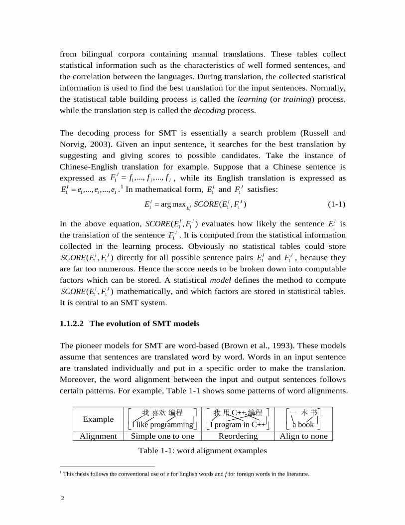
1 1( , )I JSCORE E F mathematically, and which factors are stored in statistical tables. It is central to an SMT system. 1.1.2.2 The evolution of SMT models The pioneer models for SMT are word-based (Brown et al., 1993). These models assume that sentences are translated word by word. Words in an input sentence are translated individually and put in a specific order to make the translation. Moreover, the word alignment between the input and output sentences follows certain patterns. For example, 240HTable 1-1 shows some patterns of word alignments.
Example
I like programming⎡ ⎤⎢ ⎥⎣ ⎦
我 喜欢 编程 C++I program in C++⎡ ⎤⎢ ⎥⎣ ⎦
我 用 编程 a book
⎡ ⎤⎢ ⎥⎣ ⎦
一 本 书
Alignment Simple one to one Reordering Align to none
Table 1-1: word alignment examples
1 This thesis follows the conventional use of e for English words and f for foreign words in the literature.
3
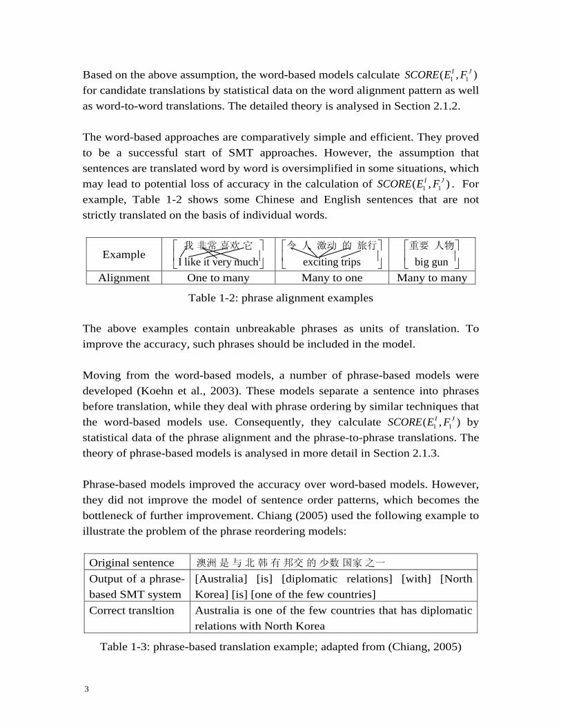
Based on the above assumption, the word-based models calculate 1 1( , )I JSCORE E F for candidate translations by statistical data on the word alignment pattern as well as word-to-word translations. The detailed theory is analysed in Section 241H2.1.2. The word-based approaches are comparatively simple and efficient. They proved to be a successful start of SMT approaches. However, the assumption that sentences are translated word by word is oversimplified in some situations, which may lead to potential loss of accuracy in the calculation of 1 1( , )I JSCORE E F . For example, 242HTable 1-2 shows some Chinese and English sentences that are not strictly translated on the basis of individual words.
Example
I like it very much⎡ ⎤⎢ ⎥⎣ ⎦
我 非常 喜欢 它
exciting trips⎡ ⎤⎢ ⎥⎣ ⎦
令 人 激动 的 旅行
big gun⎡ ⎤⎢ ⎥⎣ ⎦
重要 人物
Alignment One to many Many to one Many to many
Table 1-2: phrase alignment examples The above examples contain unbreakable phrases as units of translation. To improve the accuracy, such phrases should be included in the model. Moving from the word-based models, a number of phrase-based models were developed (Koehn et al., 2003). These models separate a sentence into phrases before translation, while they deal with phrase ordering by similar techniques that the word-based models use. Consequently, they calculate 1 1( , )I JSCORE E F by statistical data of the phrase alignment and the phrase-to-phrase translations. The theory of phrase-based models is analysed in more detail in Section 243H2.1.3. Phrase-based models improved the accuracy over word-based models. However, they did not improve the model of sentence order patterns, which becomes the bottleneck of further improvement. Chiang (2005) used the following example to illustrate the problem of the phrase reordering models:
Original sentence 澳洲 是 与 北 韩有 邦交 的少数 国家 之一 Output of a phrase-based SMT system
[Australia] [is] [diplomatic relations] [with] [North Korea] [is] [one of the few countries]
Correct transltion Australia is one of the few countries that has diplomatic relations with North Korea
Table 1-3: phrase-based translation example; adapted from (Chiang, 2005)

4
In the above example, the phrase-based SMT system translated “diplomatic relations with North Korea” and “one of the few countries” correctly. However, it failed to put the long phrases in the correct order. One possible reason is that the alignment model is based on flat reordering patterns. It may perform well with local phrase orders, but not as well with long sentences and complex orders. Based on the above observations, Chiang (2005) developed a hierarchical phrase based model. Chiang’s model evolved from the phrase-based models. However, different from simple phrases, hierarchical phrases have recursive structures. For example, “have diplomatic relation with North Korea” can be viewed as a hierarchical phrase, where “have … with …” embeds “diplomatic relation” and “North Korea”. This structure is illustrated in 244HFigure 1-1.
Figure 1-1: the hierarchical phrase structure
Now “ 1 2 f f% %与 有 ” is translated to “ 2 1 have withe e% % ”, where sub phrases 1f% and
2f% translate to 2e% and 1e% , respectively. With hierarchical structures, long phrase orders are divided into sub phrase orders, which are much simpler. 245HFigure 1-2 shows a longer example of hierarchical phrase translation.
Figure 1-2: an illustration of hierarchical phrase ordering
has with
diplomatic relation North Korea
one of that
the few countries has with
diplomatic relation North Korea
的 之一
少数国家与 有
北 韩 邦交

5
The hierarchical phrase model calculates 1 1( , )I JSCORE E F by recursive structures. It can be seen as one of the recent tree-based SMT models, and further improved the accuracy. More related SMT models are described in Section 2.1.3. From the above examples, it can be seen that SMT models has evolved towards higher levels of abstraction. The accuracy has been improved by more precise representations of structural correspondence between languages. This fact leads naturally to a question – what abstraction can best represent such correspondence? Possible answers may come from linguistics, as it is the human abstraction of languages. 1.1.3 Grammars – the provider of linguistic information Being an important part of linguistics, grammar studies the rules behind languages. Specifically, the aspect of grammar that does not concern meaning directly is called syntax, while the aspects that concern meaning include semantics and pragmatics (Allen, 1995). Grammars can be prescriptive (for example “Do not use superlative form when comparing only two objects”) or descriptive (“the word ‘anything’ is used in negative sentences and questions”). Linguists are typically more interested in descriptive grammars. In 1956, Chomsky formalized a generative way to describe grammars. Such grammars regard sentences as the result of recursive symbol generations according to certain rules. In terminology, words in a language are called terminal symbols, syntactic information such as part-of-speech (e.g. the noun, the verb etc.; Allen 1995) is called non-terminal symbols, and the rules that generate new symbols from existing symbols are called production rules. From a special starting non-terminal symbol, a sentence can be generated by recursively applying production rules to existing symbols. Chomsky classified generative grammars into four categories known as the Chomsky Hierarchy (Allen, 1995). Among these categories, the context free grammar (CFG) is frequently used to represent the syntax of English. In this grammar, every production rule takes a non-terminal symbol and generates a string of new symbols. An example CFG is shown in Figure 1-3. In this grammar, S, NP, VP, N, and V are non-terminal symbols, representing the start symbol, noun phrases, verb phrases, nouns and verbs, respectively; “I”, “like” and “C++” are terminal symbols, which are the vocabulary words in this grammar. This CFG
6
contains six production rules. For example, VP V NP is a production rule that generates string V NP (verb noun-phrase) from symbol VP (verb-phrase).
S NP VP N C++ NP N VP V NP N I V like
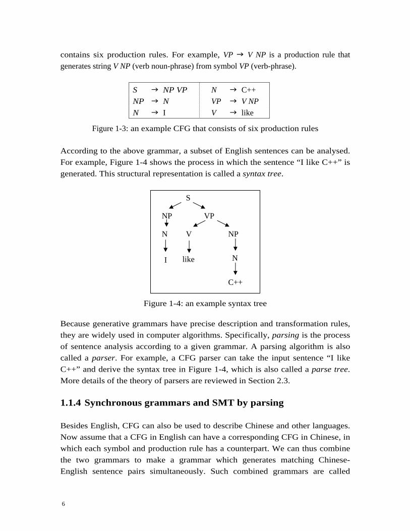
Figure 1-3: an example CFG that consists of six production rules According to the above grammar, a subset of English sentences can be analysed. For example, 248HFigure 1-4 shows the process in which the sentence “I like C++” is generated. This structural representation is called a syntax tree.
Figure 1-4: an example syntax tree
Because generative grammars have precise description and transformation rules, they are widely used in computer algorithms. Specifically, parsing is the process of sentence analysis according to a given grammar. A parsing algorithm is also called a parser. For example, a CFG parser can take the input sentence “I like C++” and derive the syntax tree in 249HFigure 1-4, which is also called a parse tree. More details of the theory of parsers are reviewed in Section 250H2.3. 1.1.4 Synchronous grammars and SMT by parsing Besides English, CFG can also be used to describe Chinese and other languages. Now assume that a CFG in English can have a corresponding CFG in Chinese, in which each symbol and production rule has a counterpart. We can thus combine the two grammars to make a grammar which generates matching Chinese-English sentence pairs simultaneously. Such combined grammars are called
NPV
S
NP VP
N
I like N
C++
7
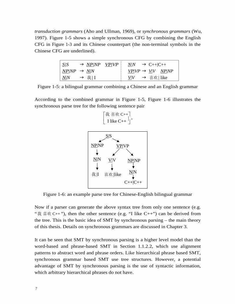
transduction grammars (Aho and Ullman, 1969), or synchronous grammars (Wu, 1997). 251HFigure 1-5 shows a simple synchronous CFG by combining the English CFG in 252HFigure 1-3 and its Chinese counterpart (the non-terminal symbols in the Chinese CFG are underlined).
S|S NP|NP VP|VP N|N C++|C++ NP|NP N|N VP|VP V|V NP|NP N|N 我 | I V|V 喜欢 | like
Figure 1-5: a bilingual grammar combining a Chinese and an English grammar According to the combined grammar in 253HFigure 1-5, 254HFigure 1-6 illustrates the synchronous parse tree for the following sentence pair
C++I like C++
⎡ ⎤⎢ ⎥⎣ ⎦
我 喜欢,
Figure 1-6: an example parse tree for Chinese-English bilingual grammar
Now if a parser can generate the above syntax tree from only one sentence (e.g. “ C++我 喜欢 ”), then the other sentence (e.g. “I like C++”) can be derived from the tree. This is the basic idea of SMT by synchronous parsing – the main theory of this thesis. Details on synchronous grammars are discussed in 255HChapter 3. It can be seen that SMT by synchronous parsing is a higher level model than the word-based and phrase-based SMT in Section 256H1.1.2.2, which use alignment patterns to abstract word and phrase orders. Like hierarchical phrase based SMT, synchronous grammar based SMT use tree structures. However, a potential advantage of SMT by synchronous parsing is the use of syntactic information, which arbitrary hierarchical phrases do not have.
NP|NPV|V
S|S
NP|NP VP|VP
N|N
我 |I 喜欢 |like N|N
C++|C++
8
The decoding algorithm for SMT by parsing is different from those models in Section 1.1.2 – the goal of the decoding search is the best synchronous tree, instead of the best translation directly. Therefore, the decoding process can be seen as a statistical parsing process (Section 2.3.2). The advantage is that existing parsing algorithms can be used to facilitate SMT research. For example, the experiments of this thesis are based on GenPar, which is the implementation of a generalised parsing algorithm (Section 2.3.3). 1.1.5 Chinese-English SMT by parsing The topic of this thesis is Chinese-English SMT by parsing. This is the first application of the SMT by parsing model in Chapter 3 to the specific language pair. On the one hand, the language-independent mathematical theory of SMT by parsing is important to the effect of translation, and the experimental output reflects the strength of weakness of the SMT model (Chapter 5). On the other hand, the effect of Chinese-English SMT is also influenced by the specific characteristics of the two languages, and language-specific processing is required for the translation. For example, a Chinese sentence is written as a continuous sequence of characters. To be processed by the SMT systems, it needs to be separated into individual words. This process is called segmentation (Jurafsky and Martin, 2000). What is more, the structural correspondence between Chinese and English is more complex than that between Indo-European language pairs. For example, phrase-based models may benefit from the strong localisation effect observed between Indo-European phrases (Tillman et al., 1997), but Chinese phrases may not have the advantage. This thesis does large-scale experiments with existing software, including the GenPar framework. Apart from the necessary software engineering work for a running system, special engineering techniques such as parallel processing are used to control the experiment progress under the time frame of this thesis. The details of these experiments are recorded in Chapter 4. The next section gives the organisation of the rest of this thesis.

9
1.2 Overview 263HChapter 2 provides the detailed background, including the mathematical theory of SMT models and MT evaluation methods. By reviewing the theory of parsers, it introduces the generalised parsing algorithm, which is used by GenPar. 264HChapter 3 introduces the synchronous grammar used by this thesis, as well as its statistical parsing model and the training and decoding process. On this basis, it introduces the theory of SMT by parsing, showing the implementation of several important algorithms by generalised parsing. 265HChapter 4 records the details of the experiments, including the software used, the corpus texts, the process of a typical experiment and brief introductions of the programs written during the process. This chapter also includes a summary of the research questions corresponding to each experiment. 266HChapter 5 discusses the research questions with the experiment results. It draws a conclusion of this thesis and gives suggestion for future work.
1.3 Contributions • Detailed exposition of the theory of SMT and SMT by parsing using the
example of Chinese-English translation, giving original analysis to important algorithms.
• First experiments on Chinese-English SMT by parsing using the GenPar
framework, with results comparable to existing language pairs using GenPar. • Demonstration that large-scale Chinese-English syntax-based SMT is possible,
by using over 3 million words of bilingual data, 32 machines and 1,000 hours of processing.
• Analysis and comparison of SMT models by novel experiments.
10
Chapter 2
Background
2.1 The theory of statistical machine translation As stated in 267HChapter 1, three important factors for SMT are the training process, the decoding process and the statistical model. Typical SMT models include the source-channel model (Brown et al., 1993) and the log-likelihood model (Och et al., 2002). This chapter uses the source-channel model for illustration. 2.1.1 The source-channel model The source-channel model originated from signal processing and information theory, and was first used in statistical natural language processing for speech recognition. It was used for SMT by Brown et al. (1993). Imagine that there is a noisy channel, through which sentences in one language are distorted into another. Now for the translation problem, the source sentences can be regarded as the result of their corresponding target sentences being passed through such an imaginary channel. The task of MT is to reconstruct the original sentences, given their distorted versions. It is done by searching for a target sentence that has the highest conditional probability given the source sentence. In mathematical form, the English translation 1
IE (i.e. 1,..., ,...i Ie e e ) for a given Chinese sentence 1
JF (i.e. 1,..., ,...j Jf f f ) is the one that satisfies:
11 1 1arg max ( | )II I J
EE P E F= (2-1)
Equation 268H2-1 is a specific version of Equation 269H1-1. This equation uses conditional probability 1 1( | )I JP E F for the ranking score 1 1( , )I JSCORE E F .
11
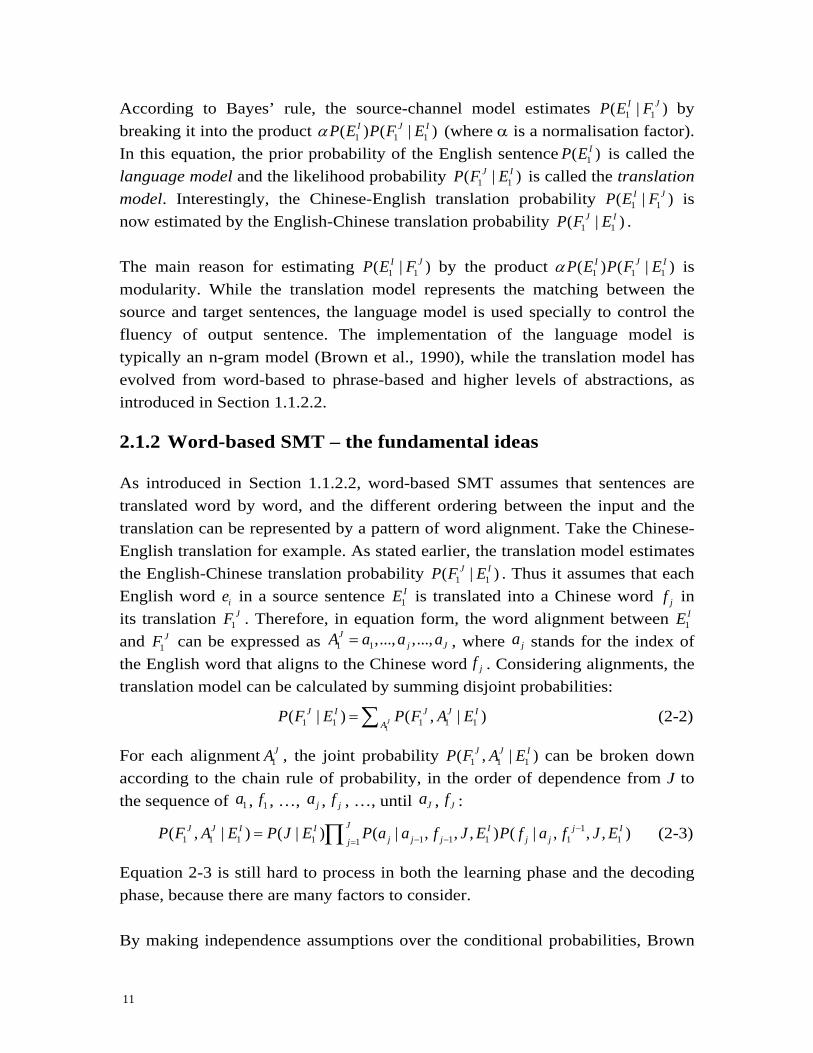
According to Bayes’ rule, the source-channel model estimates 1 1( | )I JP E F by breaking it into the product 1 1 1( ) ( | )I J IP E P F Eα (where α is a normalisation factor). In this equation, the prior probability of the English sentence 1( )IP E is called the language model and the likelihood probability 1 1( | )J IP F E is called the translation model. Interestingly, the Chinese-English translation probability 1 1( | )I JP E F is now estimated by the English-Chinese translation probability 1 1( | )J IP F E . The main reason for estimating 1 1( | )I JP E F by the product 1 1 1( ) ( | )I J IP E P F Eα is modularity. While the translation model represents the matching between the source and target sentences, the language model is used specially to control the fluency of output sentence. The implementation of the language model is typically an n-gram model (Brown et al., 1990), while the translation model has evolved from word-based to phrase-based and higher levels of abstractions, as introduced in Section 270H1.1.2.2. 2.1.2 Word-based SMT – the fundamental ideas As introduced in Section 271H1.1.2.2, word-based SMT assumes that sentences are translated word by word, and the different ordering between the input and the translation can be represented by a pattern of word alignment. Take the Chinese-English translation for example. As stated earlier, the translation model estimates the English-Chinese translation probability 1 1( | )J IP F E . Thus it assumes that each English word ie in a source sentence 1
IE is translated into a Chinese word jf in its translation 1
JF . Therefore, in equation form, the word alignment between 1IE
and 1JF can be expressed as 1 1,..., ,...,J
j JA a a a= , where ja stands for the index of the English word that aligns to the Chinese word jf . Considering alignments, the translation model can be calculated by summing disjoint probabilities:
11 1 1 1 1( | ) ( , | )J
J I J J IA
P F E P F A E=∑ (2-2)
For each alignment 1JA , the joint probability 1 1 1( , | )J J IP F A E can be broken down
according to the chain rule of probability, in the order of dependence from J to the sequence of 1a , 1f , …, ja , jf , …, until Ja , Jf :
1
1 1 1 1 1 1 1 1 11( , | ) ( | ) ( | , , , ) ( | , , , )JJ J I I I j I
j j j j jjP F A E P J E P a a f J E P f a f J E−
− −== ∏ (2-3)
Equation 272H2-3 is still hard to process in both the learning phase and the decoding phase, because there are many factors to consider. By making independence assumptions over the conditional probabilities, Brown
12
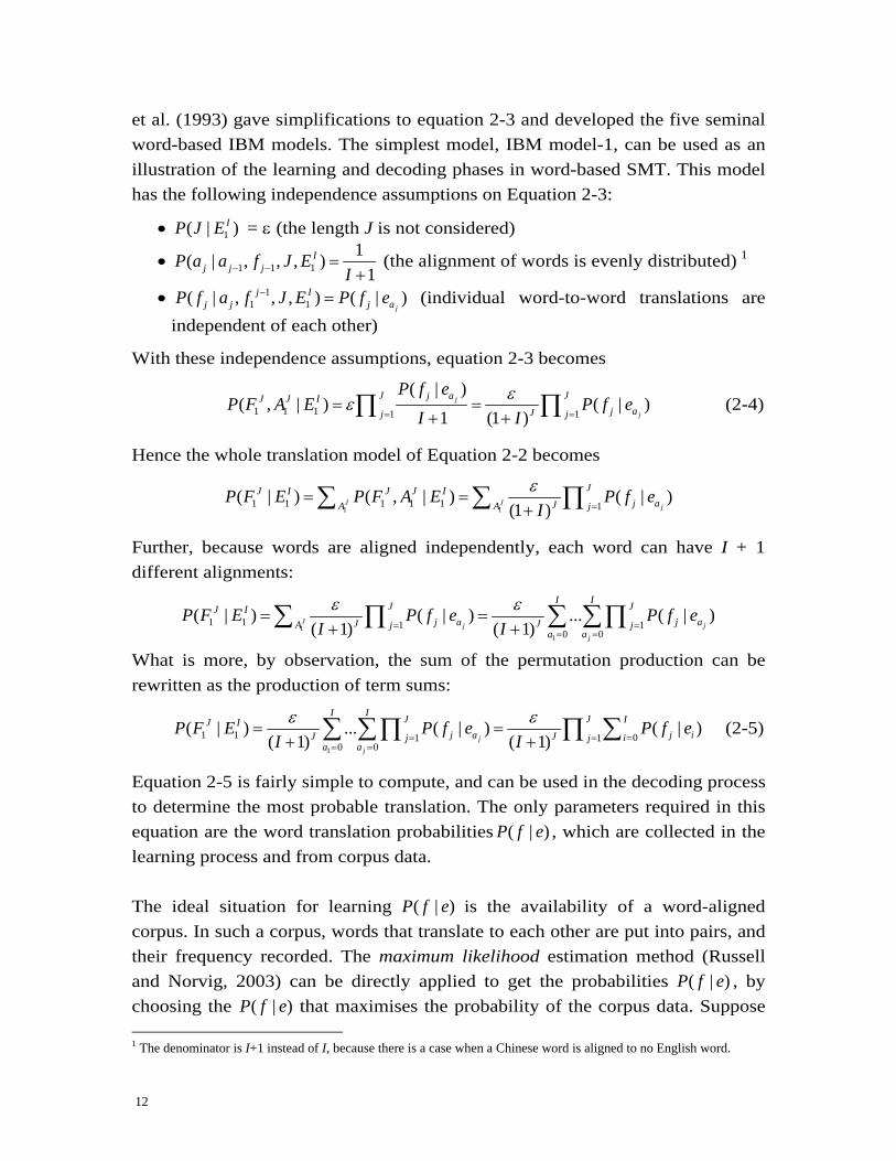
et al. (1993) gave simplifications to equation 273H2-3 and developed the five seminal word-based IBM models. The simplest model, IBM model-1, can be used as an illustration of the learning and decoding phases in word-based SMT. This model has the following independence assumptions on Equation 274H2-3:
• 1( | )IP J E = ε (the length J is not considered)
• 1 1 11( | , , , )
1I
j j jP a a f J EI− − =+
(the alignment of words is evenly distributed) 1F
1
• 11 1( | , , , ) ( | )
j
j Ij j j aP f a f J E P f e− = (individual word-to-word translations are
independent of each other)
With these independence assumptions, equation 275H2-3 becomes
1 1 1 1 1
( | )( , | ) ( | )
1 (1 )j
j
J Jj aJ J Ij aJj j
P f eP F A E P f e
I Iεε
= == =
+ +∏ ∏ (2-4)
Hence the whole translation model of Equation 276H2-2 becomes
1 11 1 1 1 1 1
( | ) ( , | ) ( | )(1 )J J j
JJ I J J Ij aJA A j
P F E P F A E P f eIε
== =
+∑ ∑ ∏
Further, because words are aligned independently, each word can have I + 1 different alignments:
11
1 1 1 10 0
( | ) ( | ) ... ( | )( 1) ( 1)J j j
j
I IJ JJ Ij a j aJ JA j j
a aP F E P f e P f e
I Iε ε
= == =
= =+ +∑ ∑ ∑∏ ∏
What is more, by observation, the sum of the permutation production can be rewritten as the production of term sums:
1
1 1 01 10 0
( | ) ... ( | ) ( | )( 1) ( 1)j
j
I I J J IJ Ij a j iJ J ij j
a aP F E P f e P f e
I Iε ε
== == =
= =+ +∑ ∑ ∑∏ ∏ (2-5)
Equation 277H2-5 is fairly simple to compute, and can be used in the decoding process to determine the most probable translation. The only parameters required in this equation are the word translation probabilities ( | )P f e , which are collected in the learning process and from corpus data. The ideal situation for learning ( | )P f e is the availability of a word-aligned corpus. In such a corpus, words that translate to each other are put into pairs, and their frequency recorded. The maximum likelihood estimation method (Russell and Norvig, 2003) can be directly applied to get the probabilities ( | )P f e , by choosing the ( | )P f e that maximises the probability of the corpus data. Suppose 1 The denominator is I+1 instead of I, because there is a case when a Chinese word is aligned to no English word.
13
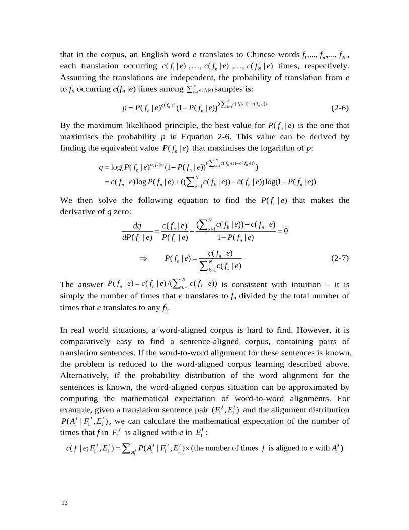
that in the corpus, an English word e translates to Chinese words 1,..., ,...,n Nf f f , each translation occurring 1( | )c f e ,…, ( | )nc f e ,…, ( | )Nc f e times, respectively. Assuming the translations are independent, the probability of translation from e to fn occurring c(fn |e) times among 1 ( | )
Nkk c f e=∑ samples is:
1
(( ( | )) ( | ))( | )( | ) (1 ( | ))N
k nn kc f e c f ec f e
n np P f e P f e =−∑= − (2-6)
By the maximum likelihood principle, the best value for ( | )nP f e is the one that maximises the probability p in Equation 278H2-6. This value can be derived by finding the equivalent value ( | )nP f e that maximises the logarithm of p:
1(( ( | )) ( | ))( | )
1
log( ( | ) (1 ( | )) )
( | ) log ( | ) (( ( | )) ( | )) log(1 ( | ))
Nk nn k
c f e c f ec f en n
Nn n k n nk
q P f e P f e
c f e P f e c f e c f e P f e
=−
=
∑= −
= + − −∑
We then solve the following equation to find the ( | )nP f e that makes the derivative of q zero:
1( ( | )) ( | )( | ) 0
( | ) ( | ) 1 ( | )
Nk nn k
n n n
c f e c f ec f edqdP f e P f e P f e
=−
= − =−
∑
1
( | )( | )( | )
nn N
kk
c f eP f ec f e
=
⇒ =∑
(2-7)
The answer 1( | ) ( | ) /( ( | ))N
n n kkP f e c f e c f e
== ∑ is consistent with intuition – it is
simply the number of times that e translates to fn divided by the total number of times that e translates to any fk. In real world situations, a word-aligned corpus is hard to find. However, it is comparatively easy to find a sentence-aligned corpus, containing pairs of translation sentences. If the word-to-word alignment for these sentences is known, the problem is reduced to the word-aligned corpus learning described above. Alternatively, if the probability distribution of the word alignment for the sentences is known, the word-aligned corpus situation can be approximated by computing the mathematical expectation of word-to-word alignments. For example, given a translation sentence pair 1 1( , )J IF E and the alignment distribution
1 1 1( | , )J J IP A F E , we can calculate the mathematical expectation of the number of times that f in 1
JF is aligned with e in 1IE :
11 1 1 1 1 1( | ; , ) ( | , ) (the number of times is aligned to with )J
J I J J I JA
c f e F E P A F E f e A= ×∑
14
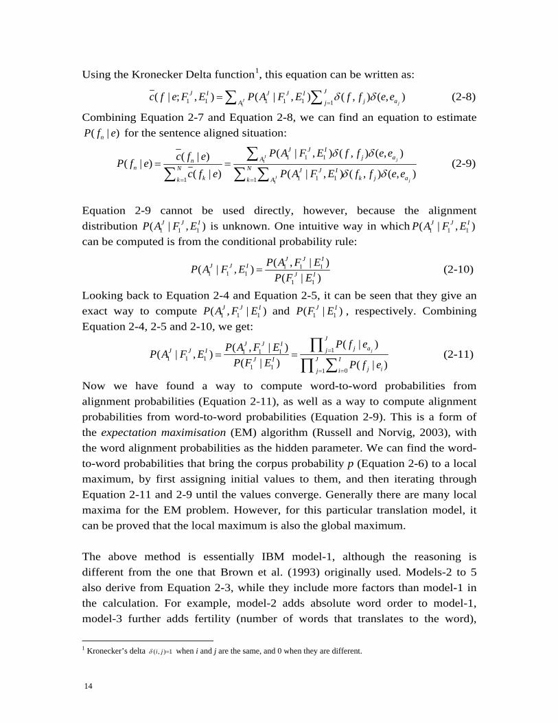
Using the Kronecker Delta function2F
1, this equation can be written as:
11 1 1 1 1 1
( | ; , ) ( | , ) ( , ) ( , )J j
JJ I J J Ij aA j
c f e F E P A F E f f e eδ δ=
=∑ ∑ (2-8)
Combining Equation 279H2-7 and Equation 280H2-8, we can find an equation to estimate ( | )nP f e for the sentence aligned situation:
1
1
1 1 1
1 1 11 1
( | , ) ( , ) ( , )( | )( | )( | ) ( | , ) ( , ) ( , )
J j
J j
J J Ij aAn
n N N J J Ik k j ak k A
P A F E f f e ec f eP f ec f e P A F E f f e e
δ δ
δ δ= =
= =∑
∑ ∑ ∑ (2-9)
Equation 281H2-9 cannot be used directly, however, because the alignment distribution 1 1 1( | , )J J IP A F E is unknown. One intuitive way in which 1 1 1( | , )J J IP A F E can be computed is from the conditional probability rule:
1 1 1
1 1 11 1
( , | )( | , )( | )
J J IJ J I
J I
P A F EP A F EP F E
=
(2-10)
Looking back to Equation 282H2-4 and Equation 283H2-5, it can be seen that they give an exact way to compute 1 1 1( , | )J J IP A F E and 1 1( | )J IP F E , respectively. Combining Equation 284H2-4, 285H2-5 and 286H2-10, we get:
11 1 11 1 1
1 1 01
( | )( , | )( | , )( | ) ( | )
j
JJ J I
j ajJ J IJ IJ I
j iij
P f eP A F EP A F EP F E P f e
=
==
= =∏∑∏
(2-11)
Now we have found a way to compute word-to-word probabilities from alignment probabilities (Equation 287H2-11), as well as a way to compute alignment probabilities from word-to-word probabilities (Equation 288H2-9). This is a form of the expectation maximisation (EM) algorithm (Russell and Norvig, 2003), with the word alignment probabilities as the hidden parameter. We can find the word-to-word probabilities that bring the corpus probability p (Equation 289H2-6) to a local maximum, by first assigning initial values to them, and then iterating through Equation 290H2-11 and 291H2-9 until the values converge. Generally there are many local maxima for the EM problem. However, for this particular translation model, it can be proved that the local maximum is also the global maximum. The above method is essentially IBM model-1, although the reasoning is different from the one that Brown et al. (1993) originally used. Models-2 to 5 also derive from Equation 292H2-3, while they include more factors than model-1 in the calculation. For example, model-2 adds absolute word order to model-1, model-3 further adds fertility (number of words that translates to the word),
1 Kronecker’s delta ( , ) 1i jδ = when i and j are the same, and 0 when they are different.
15
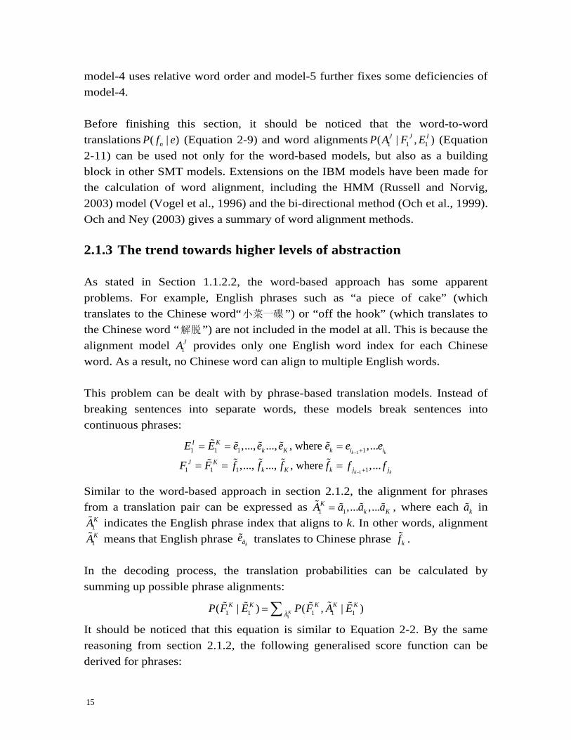
model-4 uses relative word order and model-5 further fixes some deficiencies of model-4. Before finishing this section, it should be noticed that the word-to-word translations ( | )nP f e (Equation 293H2-9) and word alignments 1 1 1( | , )J J IP A F E (Equation 294H2-11) can be used not only for the word-based models, but also as a building block in other SMT models. Extensions on the IBM models have been made for the calculation of word alignment, including the HMM (Russell and Norvig, 2003) model (Vogel et al., 1996) and the bi-directional method (Och et al., 1999). Och and Ney (2003) gives a summary of word alignment methods. 2.1.3 The trend towards higher levels of abstraction As stated in Section 295H1.1.2.2, the word-based approach has some apparent problems. For example, English phrases such as “a piece of cake” (which translates to the Chinese word“小菜一碟 ”) or “off the hook” (which translates to the Chinese word “解脱”) are not included in the model at all. This is because the alignment model 1
JA provides only one English word index for each Chinese word. As a result, no Chinese word can align to multiple English words. This problem can be dealt with by phrase-based translation models. Instead of breaking sentences into separate words, these models break sentences into continuous phrases:
11 1 1 1,..., ..., , where ,...k k
I Kk K k i iE E e e e e e e
− += = =% % % % %
11 1 1 1,..., ..., , where ,...k k
J Kk K k j jF F f f f f f f
− += = =% % % %%
Similar to the word-based approach in section 296H2.1.2, the alignment for phrases from a translation pair can be expressed as 1 1,... ,...K
k KA a a a=% % % % , where each ka% in
1KA% indicates the English phrase index that aligns to k. In other words, alignment
1KA% means that English phrase
kae%% translates to Chinese phrase kf% . In the decoding process, the translation probabilities can be calculated by summing up possible phrase alignments:
11 1 1 1 1( | ) ( , | )K
K K K K KA
P F E P F A E=∑ %%% % % %
It should be noticed that this equation is similar to Equation 297H2-2. By the same reasoning from section 298H2.1.2, the following generalised score function can be derived for phrases:

16
11 1 1 1 1 1 1 11
( | ) ( | , , ) ( | , , )KK K K K k Kk k k k kj
P F A E P a a f E P f a f E−− −=
=∏ % % %%% % % %% % %
Most current phrase-based methods are simplifications of this equation. For example, Koehn et al. (2003) used the following simplifications in their summary of phrase-based approaches:
• 1
1 1 1 1 1( | ) arg max ( , | )KK K K K K
AP F E P F A E= %
%% % % % (replace summation by maximum)
• 1 1 1 1 1( | , , ) ( | )Kk k k k kP a a f E P j i− − − −=% %% % (the phrase alignment is only dependent on
corresponding phrase positions) or 1 1| 1 |
1 1 1 1 1 1 1( | , , ) ( | ) ( 1 ) k kj iKk k k k k k kP a a f E P j i d j i α − −+ −
− − − − − −= = + − =% %% % (still further simplification – the phrase alignment is only dependent on the distance between corresponding indice)
• 11 1( | , , ) ( | )k K
k k k kP f a f E P f a− =% % %%% % (the individual phrase-to-phrase translations are independent of each other)
There are alternative ways to train a phrase-based system. Firstly, given a word alignment method (Section 299H2.1.2), phrase alignment can be derived from word-to-word alignment (Och et al., 1999, Koehn et al., 2003) – two phrases are aligned when all the words in one phrase are only aligned to words in the other. Or alternatively, phrase alignment can also be derived directly by EM machine learning methods similar to the word alignment from Section 300H2.1.2. Marcu and Wong (2002) used a (simplified) method similar to IBM model-3 to compute phrase alignments directly. The phrase-based models are able to solve the one-to-many word-alignment problem successfully. However, they still assume that sentences are translated by simple reordering. As shown in Section 301H1.1.2.2, this assumption is oversimplified for complex situations. Consequently, several tree-based models are proposed for better solutions. An example is the hierarchical phrase based model (Chiang, 2005) in 302H1.1.2.2. This model does not take use of syntactic information. The training process derives hierarchical phrase information from existing statistical word-to-word alignments. In comparison, Yamada and Knight (2001) proposed a model that uses the syntactical information of the input language. This model assumes that the translation is derived by operations over the CFG parse tree of the input sentence. It takes use of a CFG parser, and can be seen as a tree-to-string model. Meanwhile, there are also tree-to-tree models which take use of syntactic information of both the input and the translation. For example, the work of Gildea (2003) includes such models. Cowan et al. (2006) proposed a tree-to-tree model which maps the parse tree of the input language to the parse tree of

17
the translation language. As stated in Section 303H1.1.4, SMT by synchronous parsing can be seen as a specific syntax tree based SMT model. This model is based on combined syntax trees. Its decoding algorithm can benefit from existing parsing algorithms. Examples of SMT by synchronous parsing include research by Wu (1997), as well as Melamed and Wang (2005). By using the GenPar framework, this thesis uses the model of Melamed and Wang (2005). The detail of the synchronous grammar will be given in 304HChapter 3.
2.2 The evaluation of machine translation It is important to evaluate the accuracy of machine translation against fixed standards, so that the effect of different models can be seen and compared. The obvious difficulty in setting a standard for MT evaluation is the flexibility of natural language usage. For an input sentence, there can be many perfect translations. Knight and Marcu (2004) showed 12 independent English translations by human translators, given the same Chinese sentence. All of the 12 are different, yet all correct. The most accurate evaluation is human evaluation, and it is frequently used for new MT theories. However, this method is far more time consuming than automatic methods. It is difficult for human evaluators to evaluate a large sample of translated sentences. Research has shown that certain machine evaluation methods correspond reasonably well with human evaluators, and thus they are usually used for the evaluation of large test sets. This section introduces three most common automatic evaluation methods, which are used by the experiments of this thesis. 2.2.1 The Bleu metrics The Bleu metrics (Papineni et al., 2001) evaluates machine translation by comparing the output of an MT system with correct translations. Therefore, a test corpus is needed for this method, giving at least one manual translation for each test sentence. During a test, each test sentence is passed to the MT system, and the output is scored by comparison with the correct translations. This score is
18
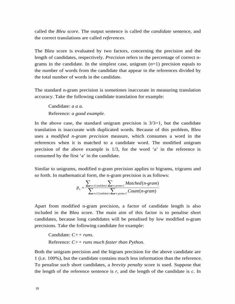
called the Bleu score. The output sentence is called the candidate sentence, and the correct translations are called references. The Bleu score is evaluated by two factors, concerning the precision and the length of candidates, respectively. Precision refers to the percentage of correct n-grams in the candidate. In the simplest case, unigram (n=1) precision equals to the number of words from the candidate that appear in the references divided by the total number of words in the candidate. The standard n-gram precision is sometimes inaccurate in measuring translation accuracy. Take the following candidate translation for example:
Candidate: a a a. Reference: a good example.
In the above case, the standard unigram precision is 3/3=1, but the candidate translation is inaccurate with duplicated words. Because of this problem, Bleu uses a modified n-gram precision measure, which consumes a word in the references when it is matched to a candidate word. The modified unigram precision of the above example is 1/3, for the word ‘a’ in the reference is consumed by the first ‘a’ in the candidate. Similar to unigrams, modified n-gram precision applies to bigrams, trigrams and so forth. In mathematical form, the n-gram precision is as follows:
{ } -
{ } -
( - )
( - )c Candidate n gram C
nc Candidate n gram C
Matched n gramp
Count n gram∈ ∈
∈ ∈
=∑ ∑∑ ∑
Apart from modified n-gram precision, a factor of candidate length is also included in the Bleu score. The main aim of this factor is to penalise short candidates, because long candidates will be penalised by low modified n-gram precisions. Take the following candidate for example:
Candidate: C++ runs. Reference: C++ runs much faster than Python.
Both the unigram precision and the bigram precision for the above candidate are 1 (i.e. 100%), but the candidate contains much less information than the reference. To penalise such short candidates, a brevity penalty score is used. Suppose that the length of the reference sentence is r, and the length of the candidate is c. In
19
equation form, the brevity penalty score is as follows:
(1 / )
1 if if c rr c
c rBP
e −
>⎧= ⎨ ≤⎩
When there are many references, r takes the length of the reference that is the closest to the length of the candidate. This length is called the effective reference length. The Bleu score combines the modified n-gram score and the brevity penalty score. When there are many test sentences in the test set, one Bleu score is calculated for all candidate translations. This is done is two steps. Firstly, the geometric average of the modified n-gram precisions pn is calculated for all n from 1 to N, using positive weights wn which sum up to 1. Secondly, the brevity penalty score is computed with the total length of all candidates and total effective reference length for all candidates. In equation form,
1
exp logN
LEU n nn
B BP w p=
⎛ ⎞= ⋅ ⎜ ⎟⎝ ⎠∑
By default, the Bleu score includes the unigram, bigram, trigram and 4-gram precisions, each having the same weight. This is done by using N=4 and wn=1/N in the above equation. Experiments have shown that the Blue metrics are generally consistent with human evaluators, and thus are useful indicators for the accuracy of machine translation. 2.2.2 The NIST metric The NIST metric (Doddington, 2002) was developed on the basis of the Bleu metrics. It focuses mainly on improving two problems of the Bleu score. Firstly, the Bleu metrics use the geometric average of modified n-gram precisions. However, because current MT systems have not reached considerable fluency, the modified n-gram precision scores may become very small for long phrases (i.e. big n). Such small scores have a potential negative effect on the overall score, which is not desired. To solve this problem, the NIST score uses the arithmetic average instead of geometric average. In this way, all modified n-gram precisions make zero or positive contribution to the overall score.
20
Secondly, the Bleu metrics weigh all n-grams equally in the modified n-gram precision score. However, some n-grams carry more useful information than others. For example, the bigram “washing machine” is considered more useful for the evaluation than the bigram “of the”. The NIST metric gives each n-gram an information weight, which is computed by:
1 11 2
1
the # of occurrences of ...( ... ) logthe # of occurrences of ...
nn
n
w wInfo w ww w
−⎛ ⎞= ⎜ ⎟
⎝ ⎠
Besides the above two differences, the NIST score also uses a special brevity penalty score. In equation form, it can be written as:
2exp log (min( ,1))sys
ref
LBP
Lβ
⎛ ⎞= ⎜ ⎟
⎝ ⎠,
where refL is the average number of words in the references, Lsys is the number of words in the candidate, and β is chosen to make BP=0.5 when the number of words in the candidate is 2/3 of the average number of words in the references. In summary, the NIST score for MT evaluation can be written as:
11...
1 1...
( ... )
(1)n
N nw w Matched
n w wn Candidate
Info w wScore BP ∈
= ∈
⎛ ⎞⎜ ⎟= ⋅⎜ ⎟⎝ ⎠
∑∑ ∑
2.2.3 The F-measure The F-measure (Turian et al., 2003) is an MT evaluation method developed independently from the Bleu and NIST metrics. In the domain of natural language processing, the term F-measure refers to a combination of precision and recall. It is commonly used for the evaluation of information retrieval systems. Suppose that the set of candidates is Y and the set of references is X, the precision, recall and F-measure are defined as follows:
| |( | )| |
X Yprecision Y XY∩
=
| |( | )| |
X Yrecall Y XY∩
=
2- precision recallF measureprecision recall× ×
=+

21
In the simplest case, the F-measure for a MT translation candidate can be based on unigram precision and recall. See 305HFigure 2-1 for an illustration of this method.
E •D •C • •I •A • •B • •C • •H A B C D E F I A B C
Figure 2-1: unigram matches; adapted from (Turian et al., 2003). In the above figure, each row represents a unigram (i.e. word) from the candidate translation (C), and each column represents a unigram from a reference (R). A dot (•) highlights the matching between a row and a column, which is called a hit. A matching is a subset of hits in which no two are in the same row or column. For the unigram case, the size of a matching can be defined as the number of hits in it. A matching with the biggest size is called a maximum matching, and is used as R C∩ for precision and recall computations. 306HFigure 2-1 shows a maximum matching with dark background. Denote the size of a maximum matching as MMS. In equation form, we have:
| ( , ) |( | )| |
MMS C Rprecision C RC
=
| ( , ) |( | )| |
MMS C Rrecall C RR
=
Therefore, from the above definitions, the unigram F-measure can be calculated. The unigram form of the F-measure treats each sentence as a bag of words. This method ignores the evaluation of the word order in the candidate translations. One way to include the word order information is weighing continuous hits (i.e. phrases) more heavily than discontinuous hits. In formal definition, a run is a sequence of hits in which both the row and the column are contiguous. For example, the matching in 307HFigure 2-1 contains three runs, each with length 1, 2 and 4 respectively. Denote a matching with M, and a run in M with r. To give
22
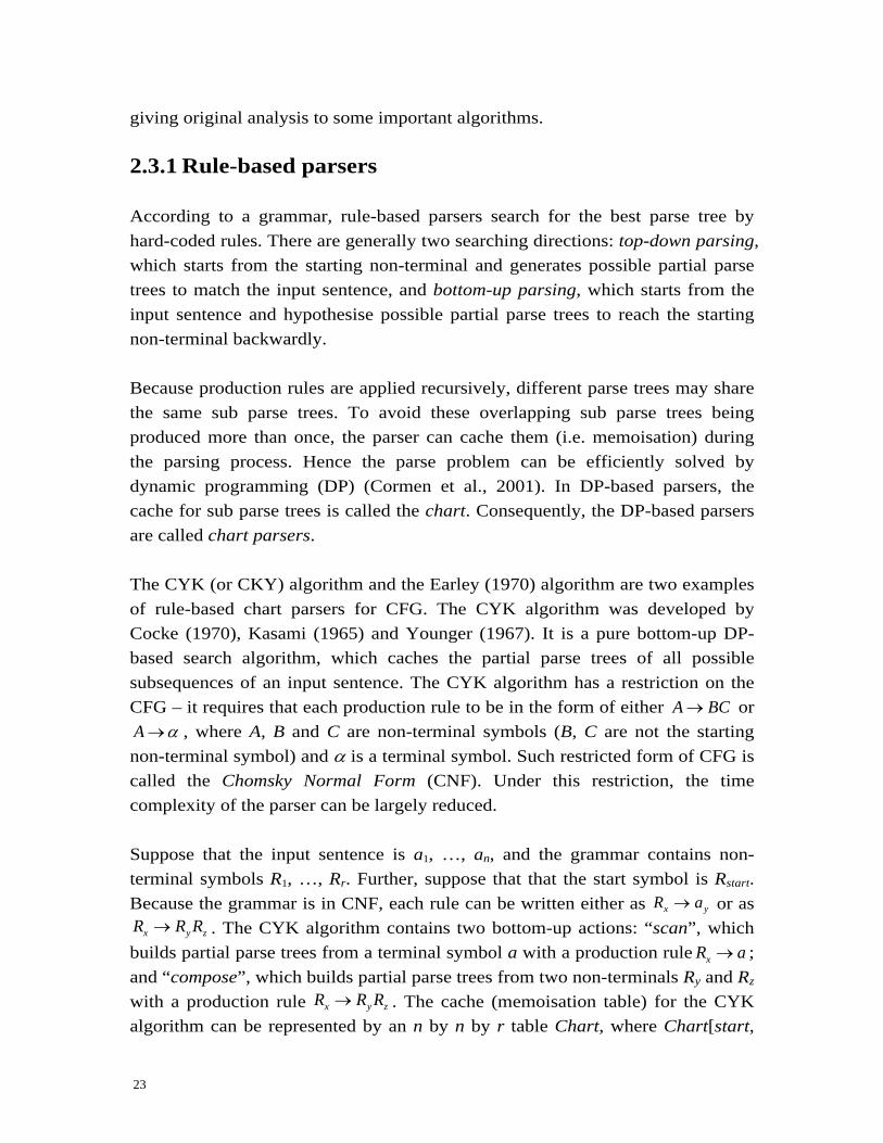
longer runs more weight, the size of matching M can be calculated by:
( ) ( )e
er M
size M length r∈
= ∑ (2-12)
In the above equation, e is the weighing factor which favours longer runs when e>1. When e=1, the F-measure is reduced to the unigram case. 2.2.4 Summary Experiments have shown that automatic evaluation methods are useful indicators of the quality of MT. However, they are not always consistent with human evaluators. Also, among different evaluation methods, some may perform comparatively better in certain cases but worse in others. For example, with the reference “programming methods”, the candidate “methods of programming” would have a comparatively low Bleu score, because it does not contain matching bigrams. The same candidate may have a better score by the unigram F-measure, because word order information is not considered by this method. Therefore, the unigram F-measure is more consistent with human evaluators in this particular example. In contrast, the candidate “methods programming of” will not be penalised by the unigram F-measure by the same reason. Therefore, the Bleu metrics will be more consistent with human evaluators in this case. The three automatic methods from Section 308H2.2.1 to Section 309H2.2.3 are currently the most commonly used for MT evaluation. In the experiments of this thesis, all three methods are applied.
2.3 The theory of parsing and generalised parsing As stated in Section 310H1.1.3, parsing refers to the process of sentence analysis in order to decide its grammatical structure. It is not only a means to bring syntactic information to SMT, but also an essential algorithm used by the synchronous parsing based SMT model. By reviewing important parsing algorithms, this section introduces the generalised parsing algorithm that GenPar implements. Similar to the development of MT algorithms (Section 311H1.1.1), natural language parsing algorithms have also evolved from rule-based to statistical approaches. Section 312H2.3.1 and Section 313H2.3.2 reviews these two approaches, respectively,
23
giving original analysis to some important algorithms. 2.3.1 Rule-based parsers According to a grammar, rule-based parsers search for the best parse tree by hard-coded rules. There are generally two searching directions: top-down parsing, which starts from the starting non-terminal and generates possible partial parse trees to match the input sentence, and bottom-up parsing, which starts from the input sentence and hypothesise possible partial parse trees to reach the starting non-terminal backwardly. Because production rules are applied recursively, different parse trees may share the same sub parse trees. To avoid these overlapping sub parse trees being produced more than once, the parser can cache them (i.e. memoisation) during the parsing process. Hence the parse problem can be efficiently solved by dynamic programming (DP) (Cormen et al., 2001). In DP-based parsers, the cache for sub parse trees is called the chart. Consequently, the DP-based parsers are called chart parsers. The CYK (or CKY) algorithm and the Earley (1970) algorithm are two examples of rule-based chart parsers for CFG. The CYK algorithm was developed by Cocke (1970), Kasami (1965) and Younger (1967). It is a pure bottom-up DP-based search algorithm, which caches the partial parse trees of all possible subsequences of an input sentence. The CYK algorithm has a restriction on the CFG – it requires that each production rule to be in the form of either A BC→ or A α→ , where A, B and C are non-terminal symbols (B, C are not the starting non-terminal symbol) and α is a terminal symbol. Such restricted form of CFG is called the Chomsky Normal Form (CNF). Under this restriction, the time complexity of the parser can be largely reduced. Suppose that the input sentence is a1, …, an, and the grammar contains non-terminal symbols R1, …, Rr. Further, suppose that that the start symbol is Rstart. Because the grammar is in CNF, each rule can be written either as x yR a→ or as
x y zR R R→ . The CYK algorithm contains two bottom-up actions: “scan”, which builds partial parse trees from a terminal symbol a with a production rule xR a→ ; and “compose”, which builds partial parse trees from two non-terminals Ry and Rz with a production rule x y zR R R→ . The cache (memoisation table) for the CYK algorithm can be represented by an n by n by r table Chart, where Chart[start,
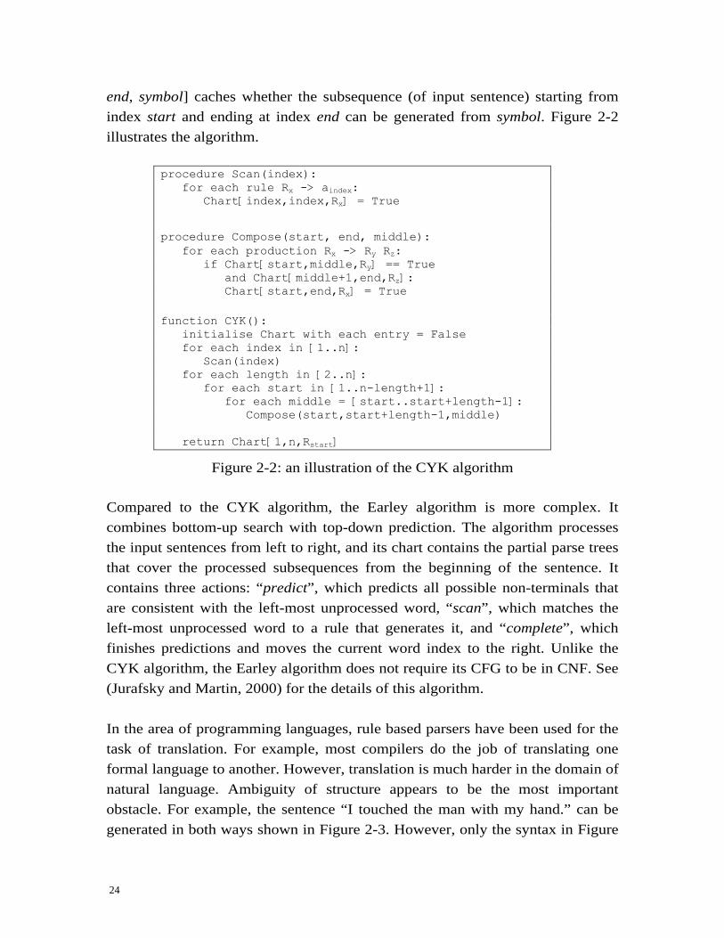
24
end, symbol] caches whether the subsequence (of input sentence) starting from index start and ending at index end can be generated from symbol. Figure 2-2 illustrates the algorithm.
procedure Scan(index): for each rule Rx -> aindex: Chart[index,index,Rx] = True procedure Compose(start, end, middle): for each production Rx -> Ry Rz: if Chart[start,middle,Ry] == True and Chart[middle+1,end,Rz]: Chart[start,end,Rx] = True function CYK(): initialise Chart with each entry = False for each index in [1..n]: Scan(index) for each length in [2..n]: for each start in [1..n-length+1]: for each middle = [start..start+length-1]: Compose(start,start+length-1,middle) return Chart[1,n,Rstart]
Figure 2-2: an illustration of the CYK algorithm Compared to the CYK algorithm, the Earley algorithm is more complex. It combines bottom-up search with top-down prediction. The algorithm processes the input sentences from left to right, and its chart contains the partial parse trees that cover the processed subsequences from the beginning of the sentence. It contains three actions: “predict”, which predicts all possible non-terminals that are consistent with the left-most unprocessed word, “scan”, which matches the left-most unprocessed word to a rule that generates it, and “complete”, which finishes predictions and moves the current word index to the right. Unlike the CYK algorithm, the Earley algorithm does not require its CFG to be in CNF. See (Jurafsky and Martin, 2000) for the details of this algorithm. In the area of programming languages, rule based parsers have been used for the task of translation. For example, most compilers do the job of translating one formal language to another. However, translation is much harder in the domain of natural language. Ambiguity of structure appears to be the most important obstacle. For example, the sentence “I touched the man with my hand.” can be generated in both ways shown in Figure 2-3. However, only the syntax in Figure
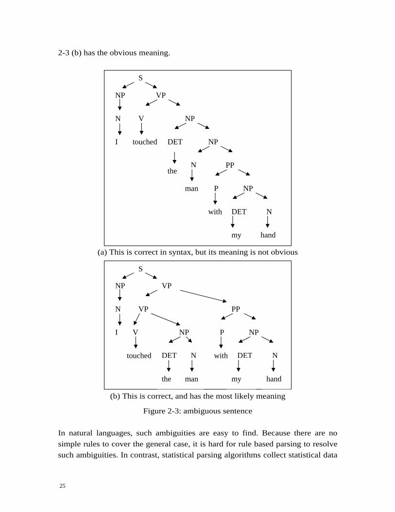
25
2-3 (b) has the obvious meaning.
(a) This is correct in syntax, but its meaning is not obvious
(b) This is correct, and has the most likely meaning
Figure 2-3: ambiguous sentence In natural languages, such ambiguities are easy to find. Because there are no simple rules to cover the general case, it is hard for rule based parsing to resolve such ambiguities. In contrast, statistical parsing algorithms collect statistical data
NPV
S
NP VP
N
I
touched N
manthe
DET N
PP
P NP
with DET
my hand
VP
NPV
S
NP VP
N
I touched
N
man
the
NPDET
N PP
P NP
with DET
my hand
26
from correctly parsed sentences, and resolves ambiguity by experience. Because of this, it has the potential to generalise better to new situations. 2.3.2 Statistical parsers The idea of statistical parsers originated in the late 1980s, when people started to investigate corpus based English grammar. This is mainly because rule-based grammars never covered the whole usage of the language, and it was doubtful whether they would ever do so. Pioneered by Geoffrey Leech and Roger Garside, linguists started to look for ways to define English grammar from examples – using human annotated corpora (Garside et al., 1987). Meanwhile, study on statistical parsing began. Similar to rule-based parsers, the statistical parsing process can be viewed as a search algorithm. However, instead of using rules to find the correct parse tree, statistical parsers select the best parse tree from possible candidates. Similar to SMT, the statistical parsing process is called a decoding process. In equation form, the decoding process finds the parse tree T for the sentence S that satisfies:
arg max ( | )TT P T S= (2-13) Similar to SMT, the detailed method to compute scores ( | )P T S is defined by a statistical model. The difference between a grammar and a model is worth noticing. A grammar defines what parse trees are allowed, and it is not confined to the scope of statistical parsers. Meanwhile, a model is the method by which candidates are evaluated in statistical parsing. One of the earliest works in statistical parsing was Sampson (1986). It used a manually designed language model based on a set of transition networks, and the stimulated annealing decoding search algorithm (Russell and Norvig, 2003). Regarding statistical parsing with CFG, an important early model is the Probabilistic Context Free Grammar (PCFG), which associates each production rule with a probability. With PCFG, a candidate parse tree can be scored by the overall probability of the rules used to generate it. Suppose each rule in a parse tree is i iLHS RHS→ , then the probability of the parse tree is:
( | ) ( | )i ii
P T S P RHS LHS=∏ (2-14)
27
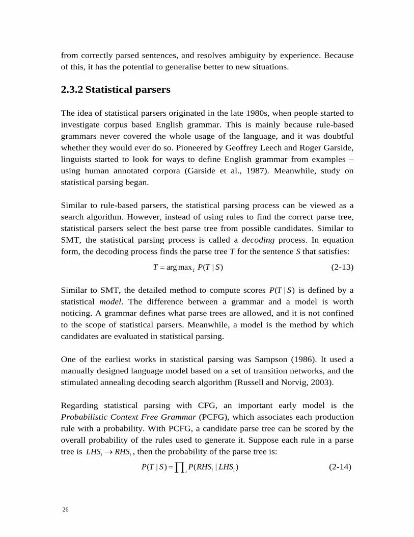
In a similar way to CFG, PCFG can also be parsed with a chart-based DP algorithm. 317HFigure 2-4 illustrates this algorithm.
procedure Scan(index): for each rule Rx → aindex: Chart[index,index,Rx] = P(aindex|Rx) procedure Compose(start, end, middle): for each production Rx -> Ry Rz: Chart[start,end,Rx] = max( Chart[start,end,Rx], Chart[start,middle,Ry] * Chart[middle+1,end,Rz] * P(Ry Rz|Rx) ) function Viterbi(Rstart): initialise Chart with each entry = 0 for each index in [1..n]: Scan(index) for each length in [2..n]: for each start in [1..n-length+1]: for each middle = [start..start+length-1]: Compose(start,start+length-1,middle) return Chart[1, n, Rstart]
Figure 2-4: an illustration of the chart parsing algorithm for PCFG (written in the same format as CYK in 318HFigure 2-2)
319HFigure 2-4 uses the same symbols as 320HFigure 2-2. However, in contrast to the CYK algorithm, Chart[start, end, symbol] for the PCFG parsing algorithm records the score for symbol to generate the fraction of input starting from index start to index end, rather than Boolean values. Correspondingly, the function Compose computes the new probability instead of the truth value. It can be seen from 321HFigure 2-4 that according to the PCFG model, the score of a parse tree is produced recursively by the factors ( | )P RHS LHS . Similar to SMT, these production rule probabilities can be derived by a training process. Training can be conducted under two different conditions. Firstly, maximum likelihood learning (Section 322H2.1.2) can be used when a corpus is available. Such a corpus containing manually parsed sentences is called a treebank. Suppose that in a treebank there are 1000 production instances starting with symbol VP, among which 600 are VP V NP. According to maximum likelihood estimation, the probability ( | )P V NP VP is the one that maximises the likelihood of the treebank,
28
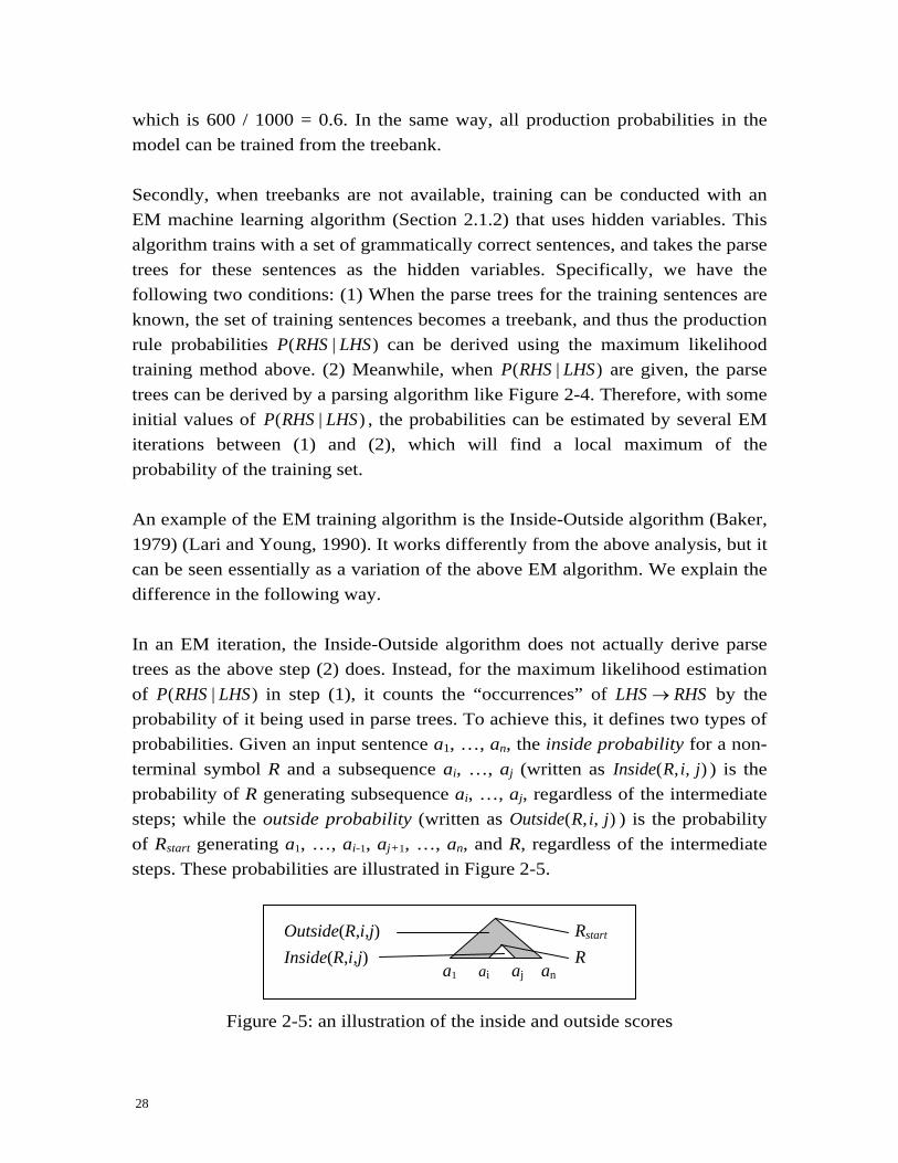
which is 600 / 1000 = 0.6. In the same way, all production probabilities in the model can be trained from the treebank. Secondly, when treebanks are not available, training can be conducted with an EM machine learning algorithm (Section 323H2.1.2) that uses hidden variables. This algorithm trains with a set of grammatically correct sentences, and takes the parse trees for these sentences as the hidden variables. Specifically, we have the following two conditions: (1) When the parse trees for the training sentences are known, the set of training sentences becomes a treebank, and thus the production rule probabilities ( | )P RHS LHS can be derived using the maximum likelihood training method above. (2) Meanwhile, when ( | )P RHS LHS are given, the parse trees can be derived by a parsing algorithm like 324HFigure 2-4. Therefore, with some initial values of ( | )P RHS LHS , the probabilities can be estimated by several EM iterations between (1) and (2), which will find a local maximum of the probability of the training set. An example of the EM training algorithm is the Inside-Outside algorithm (Baker, 1979) (Lari and Young, 1990). It works differently from the above analysis, but it can be seen essentially as a variation of the above EM algorithm. We explain the difference in the following way. In an EM iteration, the Inside-Outside algorithm does not actually derive parse trees as the above step (2) does. Instead, for the maximum likelihood estimation of ( | )P RHS LHS in step (1), it counts the “occurrences” of LHS RHS→ by the probability of it being used in parse trees. To achieve this, it defines two types of probabilities. Given an input sentence a1, …, an, the inside probability for a non-terminal symbol R and a subsequence ai, …, aj (written as ( , , )Inside R i j ) is the probability of R generating subsequence ai, …, aj, regardless of the intermediate steps; while the outside probability (written as ( , , )Outside R i j ) is the probability of Rstart generating a1, …, ai-1, aj+1, …, an, and R, regardless of the intermediate steps. These probabilities are illustrated in 325HFigure 2-5.
Figure 2-5: an illustration of the inside and outside scores
Inside(R,i,j) Outside(R,i,j)
a1 ai aj an
Rstart R
29
The above figure illustrates the full parse trees for sentence a1, …, an, as well as Inside(R,i,j) (white) and Outside(R,i,j) (grey). In these parse trees, the probability of the production rule x yR R R→ being used is:
( , , ) ( , , ) ( , , ) ( | )( ,1, )
x y x yk
start
Inside R i k Inside R k j Outside R i j P R R RInside R n
× × ×∑
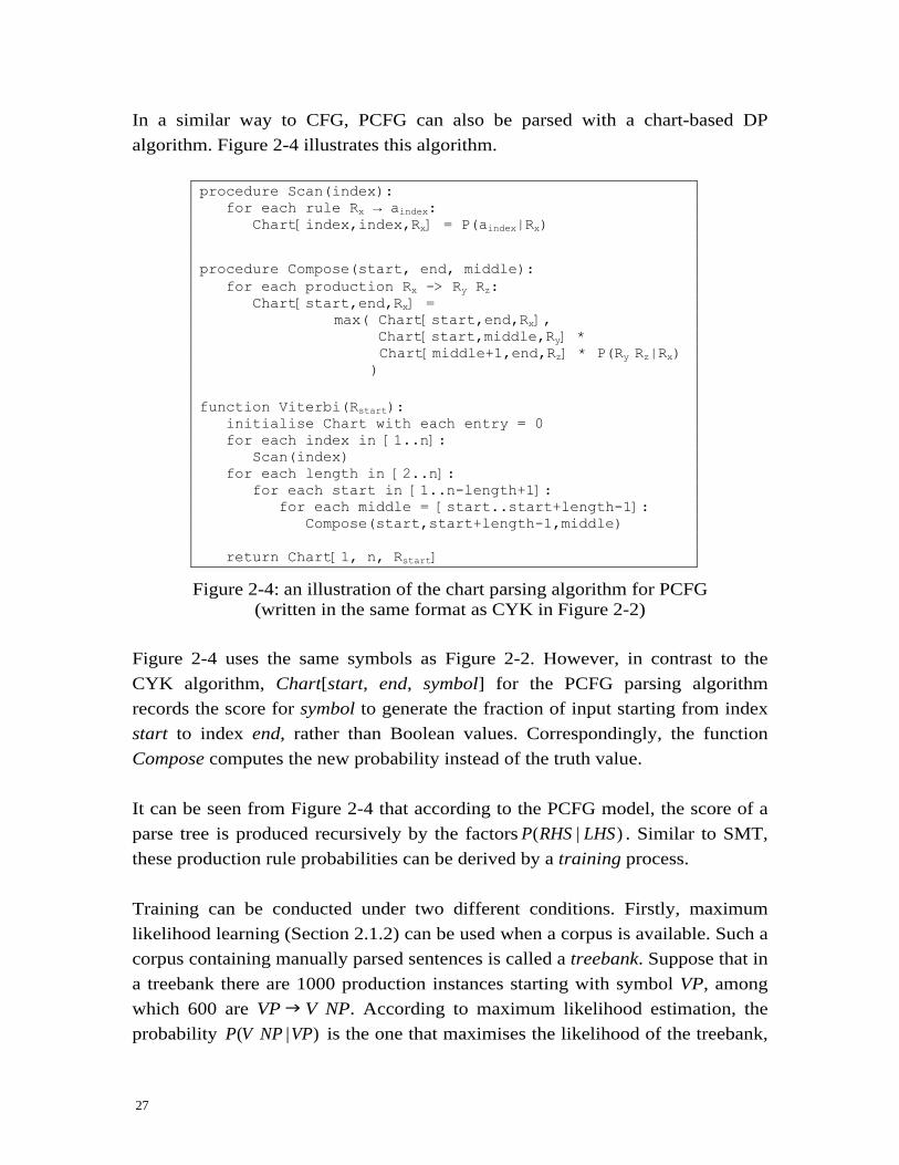
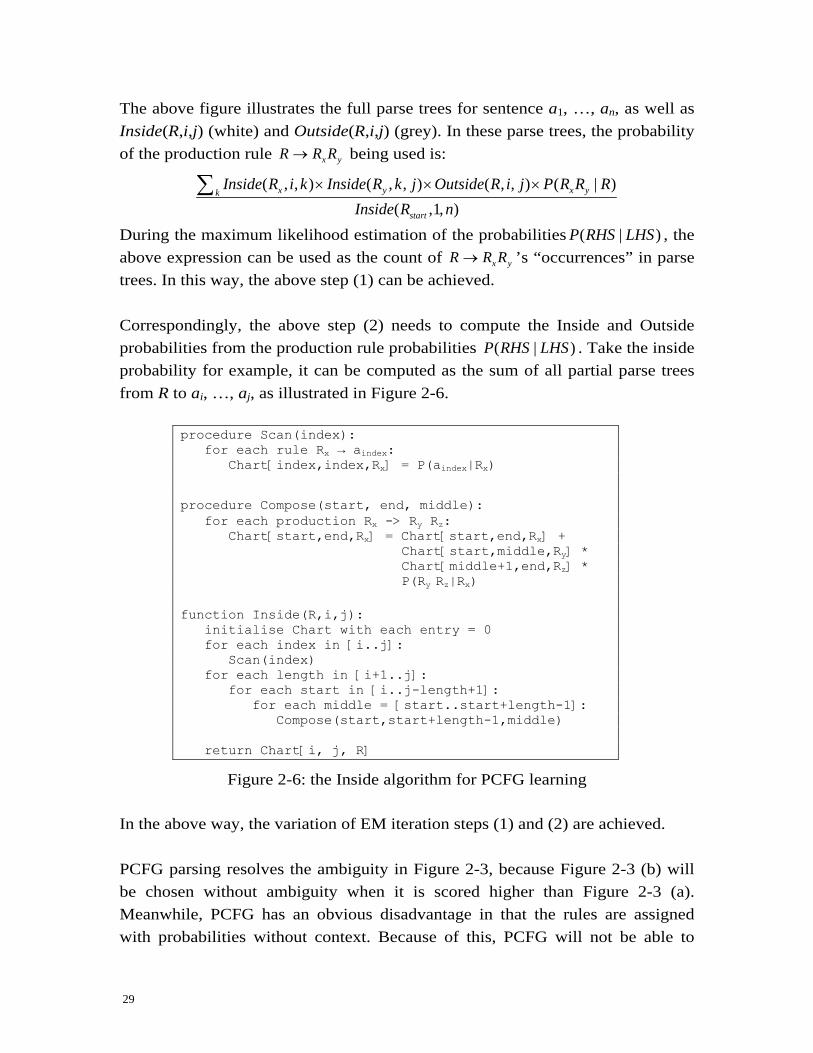
During the maximum likelihood estimation of the probabilities ( | )P RHS LHS , the above expression can be used as the count of x yR R R→ ’s “occurrences” in parse trees. In this way, the above step (1) can be achieved. Correspondingly, the above step (2) needs to compute the Inside and Outside probabilities from the production rule probabilities ( | )P RHS LHS . Take the inside probability for example, it can be computed as the sum of all partial parse trees from R to ai, …, aj, as illustrated in 326HFigure 2-6.
procedure Scan(index): for each rule Rx → aindex: Chart[index,index,Rx] = P(aindex|Rx) procedure Compose(start, end, middle): for each production Rx -> Ry Rz: Chart[start,end,Rx] = Chart[start,end,Rx] + Chart[start,middle,Ry] * Chart[middle+1,end,Rz] * P(Ry Rz|Rx) function Inside(R,i,j): initialise Chart with each entry = 0 for each index in [i..j]: Scan(index) for each length in [i+1..j]: for each start in [i..j-length+1]: for each middle = [start..start+length-1]: Compose(start,start+length-1,middle) return Chart[i, j, R]
Figure 2-6: the Inside algorithm for PCFG learning In the above way, the variation of EM iteration steps (1) and (2) are achieved. PCFG parsing resolves the ambiguity in 327HFigure 2-3, because 328HFigure 2-3 (b) will be chosen without ambiguity when it is scored higher than 329HFigure 2-3 (a). Meanwhile, PCFG has an obvious disadvantage in that the rules are assigned with probabilities without context. Because of this, PCFG will not be able to
30
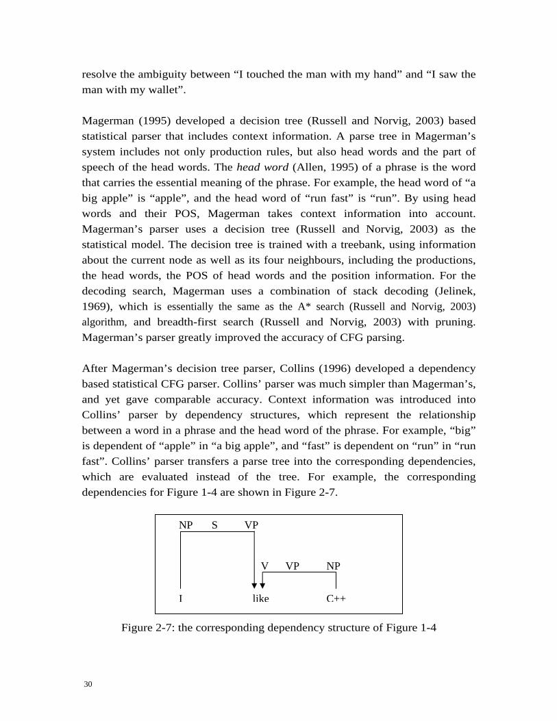
resolve the ambiguity between “I touched the man with my hand” and “I saw the man with my wallet”. Magerman (1995) developed a decision tree (Russell and Norvig, 2003) based statistical parser that includes context information. A parse tree in Magerman’s system includes not only production rules, but also head words and the part of speech of the head words. The head word (Allen, 1995) of a phrase is the word that carries the essential meaning of the phrase. For example, the head word of “a big apple” is “apple”, and the head word of “run fast” is “run”. By using head words and their POS, Magerman takes context information into account. Magerman’s parser uses a decision tree (Russell and Norvig, 2003) as the statistical model. The decision tree is trained with a treebank, using information about the current node as well as its four neighbours, including the productions, the head words, the POS of head words and the position information. For the decoding search, Magerman uses a combination of stack decoding (Jelinek, 1969), which is essentially the same as the A* search (Russell and Norvig, 2003) algorithm, and breadth-first search (Russell and Norvig, 2003) with pruning. Magerman’s parser greatly improved the accuracy of CFG parsing. After Magerman’s decision tree parser, Collins (1996) developed a dependency based statistical CFG parser. Collins’ parser was much simpler than Magerman’s, and yet gave comparable accuracy. Context information was introduced into Collins’ parser by dependency structures, which represent the relationship between a word in a phrase and the head word of the phrase. For example, “big” is dependent of “apple” in “a big apple”, and “fast” is dependent on “run” in “run fast”. Collins’ parser transfers a parse tree into the corresponding dependencies, which are evaluated instead of the tree. For example, the corresponding dependencies for Figure 1-4 are shown in Figure 2-7.
Figure 2-7: the corresponding dependency structure of Figure 1-4
I like C++
NPV VP
NP S VP
31
Before the dependencies are evaluated, Collins’ parser reduces non-recursive noun phrases (called baseNPs) in the input sentence into their head words. For example, “a big apple” will be reduced to “apple” before parsing. This helps to improve the accuracy of dependency structures by removing dependency within noun phrases. With basedNPs considered, Collins’ parser works in two steps. Firstly identify the baseNPs B from the sentence, then analyse the dependencies D on the basis of B. In equation form, T=(B,D) and
( | ) ( , | ) ( | ) ( | , )P T S P B D S P B S P D B S= =
With a treebank, the probabilities for the dependencies can be trained with the relative frequencies. Thus Collins’ parser is comparatively very quick to train. Collins’ parser uses a simple bottom-up chart parsing algorithm, and has reasonable efficiency. Collins (1997) further improved the parser by proposing three different statistical models. Other statistical models for lexicalised PCFG include the maximum entropy based model (Charniak, 2000). With re-ranking and other techniques, the model reaches the best accuracy in the literature (McClosky et al., 2006). 2.3.3 Generalised parsing Like most AI algorithms, parsing is essentially a search problem. In this sense, both rule based parsing and statistical parsing are under the same framework. Summarising similarities among parsers, Goodman (1998) outlined a semiring parsing algorithm which summarises a wide range of problems including both rule based parsing and probabilistic parsing. A semiring (Rosenfeld, 1968) is an algebraic set that is closed under two operators ⊕ and ⊗, and that conform to a set of restrictions, such as the identity elements 0 and 1, and the distribution of ⊗ over ⊕. For example, non-negative integers make a semiring, with numerical addition being ⊕ and numerical multiplication being ⊗. 0 and 1 are the identity elements for ⊕ and ⊗, respectively. Boolean values also make a semiring, with AND being ⊕ and OR being ⊗. False and True are the identity elements for ⊕ and ⊗, respectively. The same concept of semiring can be used to describe different mathematical sets. Goodman (1998) utilised this idea, and used the same general parsing algorithm to describe different specific parsing algorithms. The basis of semiring parsing is
32
the similarity between parsers. For example, 333HFigure 2-2, 334HFigure 2-4 and 335HFigure 2-6, as written in similar structures, shows the similarity between the three algorithms. As Goodman pointed out, they can be viewed as the same generalised parsing algorithm under different semirings. For a specific parser, the semiring defines the specific method for scoring candidates in the search algorithm. Observing the Compose function, it can be seen that the semiring for the CYK algorithm has the Boolean set, with (∧, ∨) as the operators (⊕,⊗). Meanwhile, the semirings for the Viterbi and Inside algorithms both have the non-negative floating point set, while they have (+, max) and (+, ×) as (⊕, ⊗), respectively. To put such generalisation into practical efficiency, Melamed (2005) suggested a generalised parsing algorithm that is based on semiring parsing. It consists of five components: a grammar, a logic, a semiring, a search strategy and a termination condition. As the name suggests, grammar defines terminal and non-terminal symbols, as well as a set of production rules. Logic defines the mechanism how the parser runs by generating new partial parse trees. The semiring defines how partial parse trees are scored, the search strategy defines the order in which partial parse trees are processed, and the termination condition defines when to stop the logic necessarily. Using G for the grammar, L for the logic, R for the semiring (⊕R and ⊗R for the operators and 0R and 1R for the identity elements), S for the search strategy and C for the termination condition, the generalised parsing algorithm can be illustrated in brief as 336HFigure 2-8.
initialise the R value for symbols and production rules from G while C isn’t met: get a set of symbols X by S pass X to L to generate a set of symbols Y assign R value for symbols in Y
Figure 2-8: generalised parsing With one or many of the five components specifically defined, the generalised parser can be turned into a specific parser such as the CYK parser. In this way the generalised parser saves development time by module reusing. Starting with the synchronous grammar for the experiments, the next chapter shows how this generalised parsing algorithm can be used to facilitate the implementation of various algorithms in SMT by parsing.
33
Chapter 3
The theory of SMT by parsing
3.1 Statistical GMTG and its generalised parsing The concept of SMT by parsing was introduced in Section 337H1.1.4, using a simple synchronous CFG. Moving from this oversimplified example, this section derives the generalised multitext grammar (GMTG; Melamed et al., 2004), which is able to express more general parallel structures, and is used in the experiments. Then it introduces the probabilistic version of this grammar, and the corresponding statistical learning and decoding (parsing) algorithms with generalised parsing. 3.1.1 Generalised multitext grammar (GMTG) 3.1.1.1 Reordering The grammar in 338HFigure 1-5 combines an English CFG with its exact counterpart in Chinese. It can be used to analyse the following sentence pair:
C++I like C++
⎡ ⎤⎢ ⎥⎣ ⎦
我 喜欢
However, the same type of grammar is unable to describe sentence pairs in different word order. Take the following sentence pair for example:
C++I like C++ very much⎡ ⎤⎢ ⎥⎣ ⎦
我 非常 喜欢
As illustrated in 339HFigure 3-1, the order of the Chinese verb phrase “ C++非常 喜欢 ” is adverb phrase (“非常 ”) + verb phrase (“ C++喜欢 ”), while the order of the English translation is verb phrase (“like C++”) + adverb phrase (“very much”). Therefore, the Chinese production rule VP ADVP VP and the corresponding English production rule VP VP ADVP cannot be combined directly.

34
(a) The Chinese parse tree (b) The English parse tree
Figure 3-1: an illustration of constituent reordering between Chinese and English In vector form, we need to combine the following production rules:
VP ADVP VPVP VP ADVP
→⎡ ⎤⎢ ⎥→⎣ ⎦
To solve this problem, symbol ordering must be included into the synchronous grammar. GMTG (Melamed and Wang, 2005) introduces the concept of precedence array vector (PAV) to describe such ordering. For example, the above CFG production rules can be combined into one rule in GMTG as:
[1,2]
[2,1]VP ADVP VPVP ADVP VP
⎡ ⎤ ⎡ ⎤→ ⎢ ⎥ ⎢ ⎥
⎣ ⎦ ⎣ ⎦><
On the right hand side of this production rule, symbol joins a PAV (the first vector) with a symbol vector (the second vector). In this action, each row in the PAV (called a precedence array) defines the order of the corresponding symbols in the symbol vector. For example, the precedence array and the non-terminal symbols in the second row (i.e. [2,1] and [ADVP VP]) are joined to give [VP ADVP]. In this way, reordering can be expressed in the production rules. In a GMTG production rule, each column in the symbol vector represents corresponding symbols in the two languages, and is called a link. The left hand side of a GMTG production rule is also a link. In the above production rule, the links are [VP VP], [ADVP ADVP], and [VP VP]. Though each link has the same
NPV
S
NP VP
N
我
喜欢 N
C++
ADVP
非常 NPV
S
NP VP
N
I
like N
C++
VP ADVP
very much
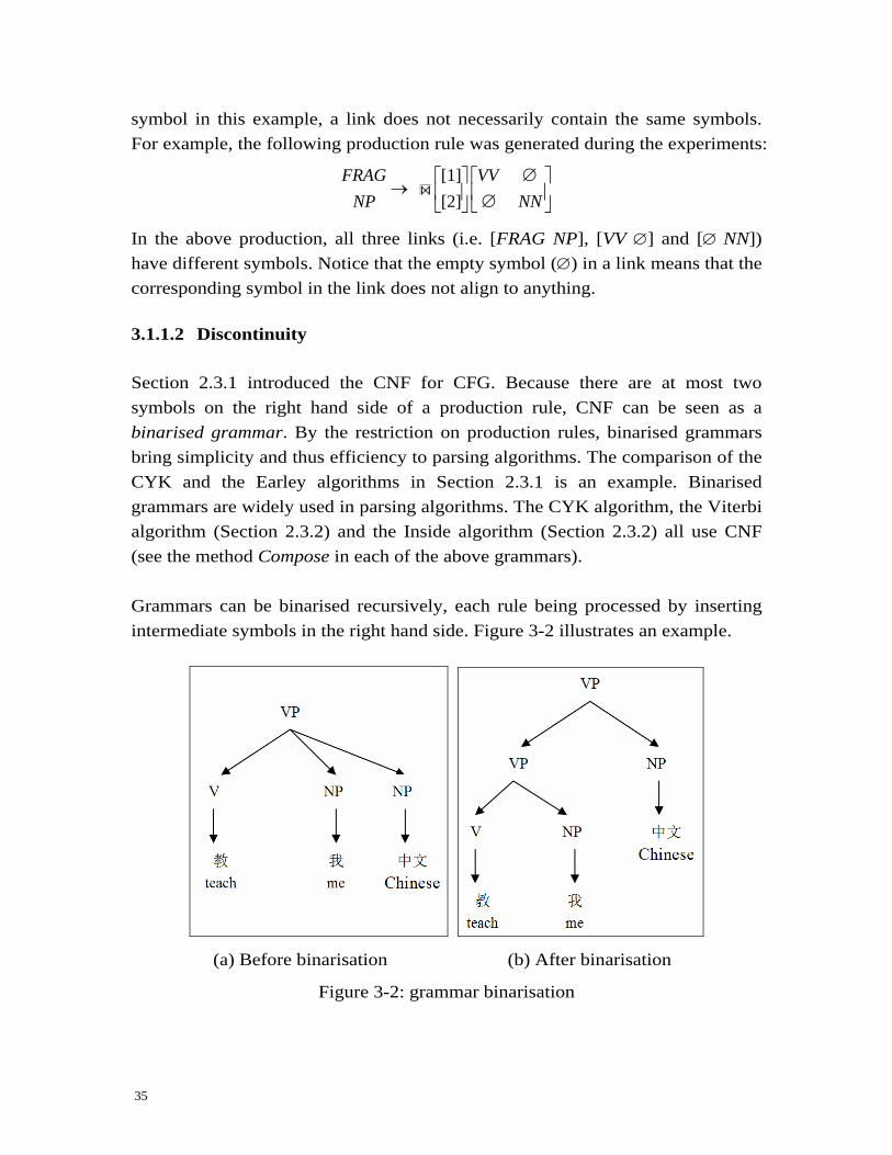
35
symbol in this example, a link does not necessarily contain the same symbols. For example, the following production rule was generated during the experiments:
[1]
[2]FRAG VV
NP NN∅⎡ ⎤ ⎡ ⎤
→ ⎢ ⎥ ⎢ ⎥∅⎣ ⎦ ⎣ ⎦><
In the above production, all three links (i.e. [FRAG NP], [VV ∅] and [∅ NN]) have different symbols. Notice that the empty symbol (∅) in a link means that the corresponding symbol in the link does not align to anything. 3.1.1.2 Discontinuity Section 340H2.3.1 introduced the CNF for CFG. Because there are at most two symbols on the right hand side of a production rule, CNF can be seen as a binarised grammar. By the restriction on production rules, binarised grammars bring simplicity and thus efficiency to parsing algorithms. The comparison of the CYK and the Earley algorithms in Section 341H2.3.1 is an example. Binarised grammars are widely used in parsing algorithms. The CYK algorithm, the Viterbi algorithm (Section 342H2.3.2) and the Inside algorithm (Section 343H2.3.2) all use CNF (see the method Compose in each of the above grammars). Grammars can be binarised recursively, each rule being processed by inserting intermediate symbols in the right hand side. 344HFigure 3-2 illustrates an example.
(a) Before binarisation (b) After binarisation
Figure 3-2: grammar binarisation
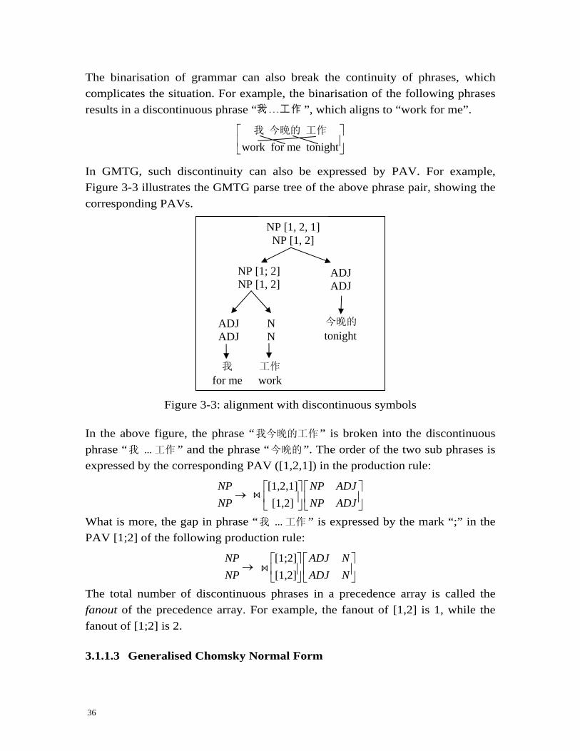
36
The binarisation of grammar can also break the continuity of phrases, which complicates the situation. For example, the binarisation of the following phrases results in a discontinuous phrase “ ”, which aligns to “work for me”.
work for me tonight⎡ ⎤⎢ ⎥⎣ ⎦
我 今晚的 工作
In GMTG, such discontinuity can also be expressed by PAV. For example, 345HFigure 3-3 illustrates the GMTG parse tree of the above phrase pair, showing the corresponding PAVs.
Figure 3-3: alignment with discontinuous symbols
In the above figure, the phrase “我今晚的工作” is broken into the discontinuous phrase “ ... 我 工作 ” and the phrase “今晚的”. The order of the two sub phrases is expressed by the corresponding PAV ([1,2,1]) in the production rule:
[1,2,1]
[1,2]NP NP ADJNP NP ADJ
⎡ ⎤ ⎡ ⎤→ ⎢ ⎥ ⎢ ⎥
⎣ ⎦ ⎣ ⎦><
What is more, the gap in phrase “ ... 我 工作 ” is expressed by the mark “;” in the PAV [1;2] of the following production rule:
[1;2]
[1,2]NP ADJ NNP ADJ N
⎡ ⎤ ⎡ ⎤→ ⎢ ⎥ ⎢ ⎥
⎣ ⎦ ⎣ ⎦><
The total number of discontinuous phrases in a precedence array is called the fanout of the precedence array. For example, the fanout of [1,2] is 1, while the fanout of [1;2] is 2. 3.1.1.3 Generalised Chomsky Normal Form
ADJ ADJ
NP [1, 2, 1]NP [1, 2]
今晚的
tonightADJ ADJ
N N
我 for me
工作
work
NP [1; 2]NP [1, 2]

37
For formal definition, this thesis uses the Generalised Chomsky Normal Form (GCNF) (Melamed et al., 2004) to express binarised GMTG, consistent with the software system for the experiments. Like CNF, GCNF defines two types of production rules – the non-terminating productions, which involve only non-terminal symbols, and the terminating productions, which involve terminal symbols. The non-terminating productions join a PAV and a symbol vector on the right hand side. Example non-terminating rules can be:
[1]
[2]FRAG VV
NP NN∅⎡ ⎤ ⎡ ⎤
→ ⎢ ⎥ ⎢ ⎥∅⎣ ⎦ ⎣ ⎦><
[1,2,1]or
[1,2]NP NP ADJNP NP ADJ
⎡ ⎤ ⎡ ⎤→ ⎢ ⎥ ⎢ ⎥
⎣ ⎦ ⎣ ⎦><
In comparison, a terminating production has only one terminal symbol link on the right hand side, and therefore no PAV. What is more, it has only one language active, and uses empty symbols (∅) for the other language. Examples include:
or V like
N ∅ ∅→ →
∅ ∅我
According to the above definition, the GCNF syntax tree for 346HFigure 1-6 is:
Figure 3-4: the GCNF format of 347HFigure 1-6
∅ V
喜欢
∅ C++∅
∅ like
我 ∅
∅I
V ∅ N | ∅
∅| N N ∅
∅ N
V [1]V [2]
NP | NP N ∅
∅N
NP [1] NP [2]
NP [1] NP [2]
VP [1,2]VP [1,2]
S [1,2] S [1,2]
∅C++
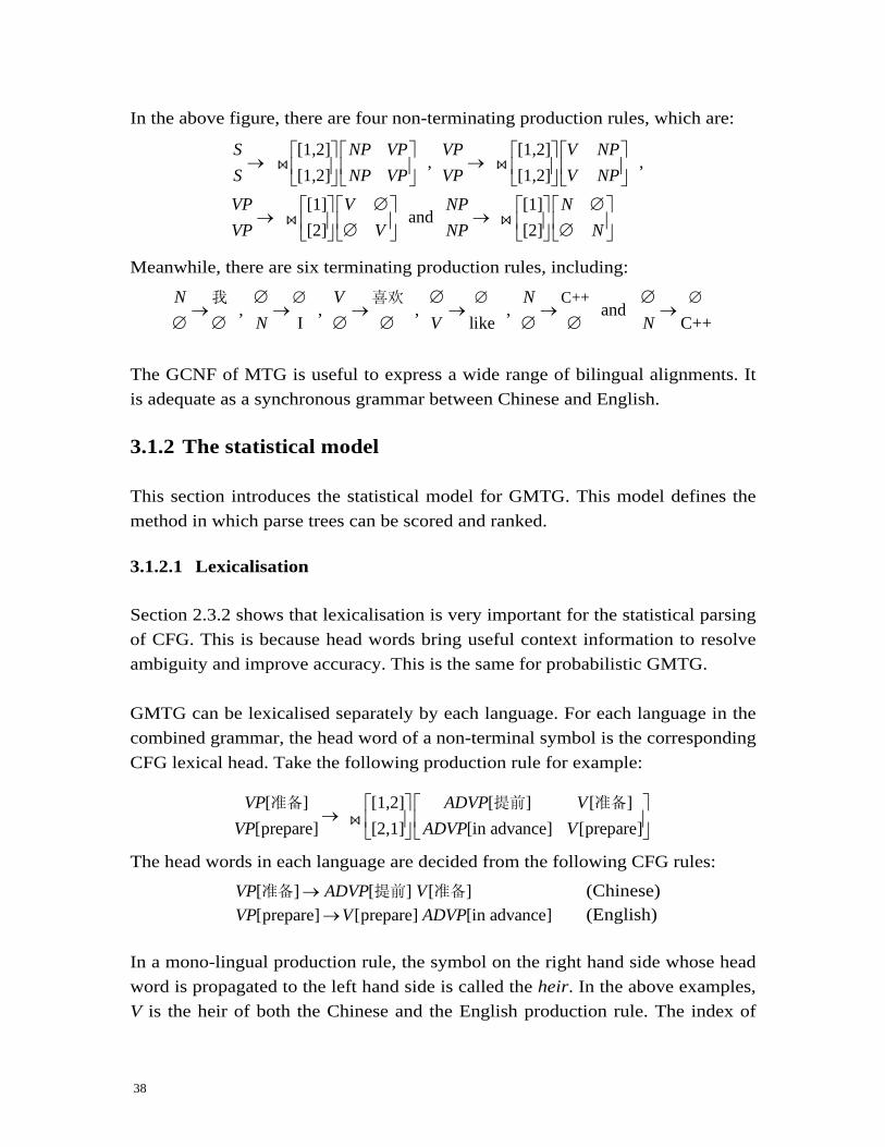
38
In the above figure, there are four non-terminating production rules, which are:
[1,2] [1,2] , ,
[1,2] [1,2]
[1] [1] and
[2] [2]
S NP VP VP V NPS NP VP VP V NP
VP V NP NVP V NP N
⎡ ⎤ ⎡ ⎤ ⎡ ⎤ ⎡ ⎤→ →⎢ ⎥ ⎢ ⎥ ⎢ ⎥ ⎢ ⎥
⎣ ⎦ ⎣ ⎦ ⎣ ⎦ ⎣ ⎦∅ ∅⎡ ⎤ ⎡ ⎤ ⎡ ⎤ ⎡ ⎤
→ →⎢ ⎥ ⎢ ⎥ ⎢ ⎥ ⎢ ⎥∅ ∅⎣ ⎦ ⎣ ⎦ ⎣ ⎦ ⎣ ⎦
>< ><
>< ><
Meanwhile, there are six terminating production rules, including:
C++ , , , , and
I like C++N V N
N V N∅ ∅ ∅∅ ∅ ∅
→ → → → → →∅ ∅ ∅ ∅ ∅ ∅
我 喜欢
The GCNF of MTG is useful to express a wide range of bilingual alignments. It is adequate as a synchronous grammar between Chinese and English. 3.1.2 The statistical model This section introduces the statistical model for GMTG. This model defines the method in which parse trees can be scored and ranked. 3.1.2.1 Lexicalisation Section 348H2.3.2 shows that lexicalisation is very important for the statistical parsing of CFG. This is because head words bring useful context information to resolve ambiguity and improve accuracy. This is the same for probabilistic GMTG. GMTG can be lexicalised separately by each language. For each language in the combined grammar, the head word of a non-terminal symbol is the corresponding CFG lexical head. Take the following production rule for example:
[ ] [1,2] [ ] [ ]
[prepare] [2,1] [in advance] [prepare]VP ADVP V
VP ADVP V⎡ ⎤ ⎡ ⎤
→ ⎢ ⎥ ⎢ ⎥⎣ ⎦ ⎣ ⎦
><
准备 提前 准备
The head words in each language are decided from the following CFG rules:
[ ] [ ] [ ]VP ADVP V→准备 提前 准备 (Chinese) [prepare] [prepare] [in advance]VP V ADVP→ (English) In a mono-lingual production rule, the symbol on the right hand side whose head word is propagated to the left hand side is called the heir. In the above examples, V is the heir of both the Chinese and the English production rule. The index of

39
heir is called the heir role. For example, the heir role for the above Chinese and English production rules are 2 and 1, respectively. For a GMTG production rule, combining the heir role for each language makes an heir role vector. For example, the heir role vector of the above example is [2,1]. Similarly, combining the symbol heir in each language makes a heir vector. In the above example, the heir vector is the second column in the symbol vector: [ [ ], [prepare]]V V准备 . 3.1.2.2 Six events to calculate production probability Similar to PCFG, the probability of a GMTG parse tree can be computed by the overall probability of the production rules that generate it. Suppose that a parse tree is generated by a set of productions LHSi RHSi. In equation form, the probability of the tree is:
( | ) ( | )i iiP T S P RHS LHS=∏
Now we define a statistical model by breaking the probability of each production rule into smaller factors, so that it becomes more computable. Consider the production LHS RHS, where RHS has v links (v=1 or v=2). When v=1, this production is a terminating production (Section 349H3.1.1.1). In this case, RHS is just the lexical heads from LHS. Thus ( | , 1) 1P RHS LHS v = = , and
( , 1| )P RHS v LHS= = ( 1| ) ( | , 1)P v LHS P RHS LHS v= = = ( 1| )P v LHS=
When v=2, this production is a non-terminating production, and RHS consists of a precedence array vector PAV and a symbol vector SYM (Section 350H3.1.1.1). Denote the heir role vector with hrv, and the corresponding heir vector with HV (Section 351H3.1.2.1). Also, denote the dependencies with D. (These dependencies are decided in each dimension separately, in the same way as Section 352H2.3.2) According to the chain rule, the probability
( , 2 | )P RHS v LHS= = ( 2 | ) ( , | , 2)P v LHS P SYM PAV LHS v= = = ( 2 | ) ( | , 2) ( | , , 2)P v LHS P SYM LHS v P PAV SYM LHS v= = = = ( 2 | ) ( | , 2) ( | , , 2)P v LHS P hrv LHS v P HV hrv LHS v= = = ( | , , , 2) ( | , , 2)P D HV hrv LHS v P PAV SYM LHS v= = ( 3-1)
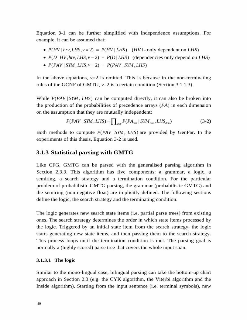
40
Equation 353H3-1 can be further simplified with independence assumptions. For example, it can be assumed that:
• ( | , , 2) ( | )P HV hrv LHS v P HV LHS= = (HV is only dependent on LHS) • ( | , , , 2) ( | )P D HV hrv LHS v P D LHS= = (dependencies only depend on LHS) • ( | , , 2) ( | , )P PAV SYM LHS v P PAV SYM LHS= = In the above equations, v=2 is omitted. This is because in the non-terminating rules of the GCNF of GMTG, v=2 is a certain condition (Section 354H3.1.1.3). While ( | , )P PAV SYM LHS can be computed directly, it can also be broken into the production of the probabilities of precedence arrays (PA) in each dimension on the assumption that they are mutually independent:
( | , ) ( | , )dim dim dimdim
P PAV SYM LHS P PA SYM LHS=∏ (3-2)
Both methods to compute ( | , )P PAV SYM LHS are provided by GenPar. In the experiments of this thesis, Equation 355H3-2 is used. 3.1.3 Statistical parsing with GMTG Like CFG, GMTG can be parsed with the generalised parsing algorithm in Section 356H2.3.3. This algorithm has five components: a grammar, a logic, a semiring, a search strategy and a termination condition. For the particular problem of probabilistic GMTG parsing, the grammar (probabilistic GMTG) and the semiring (non-negative float) are implicitly defined. The following sections define the logic, the search strategy and the terminating condition. The logic generates new search state items (i.e. partial parse trees) from existing ones. The search strategy determines the order in which state items processed by the logic. Triggered by an initial state item from the search strategy, the logic starts generating new state items, and then passing them to the search strategy. This process loops until the termination condition is met. The parsing goal is normally a (highly scored) parse tree that covers the whole input span. 3.1.3.1 The logic Similar to the mono-lingual case, bilingual parsing can take the bottom-up chart approach in Section 357H2.3 (e.g. the CYK algorithm, the Viterbi algorithm and the Inside algorithm). Starting from the input sentence (i.e. terminal symbols), new
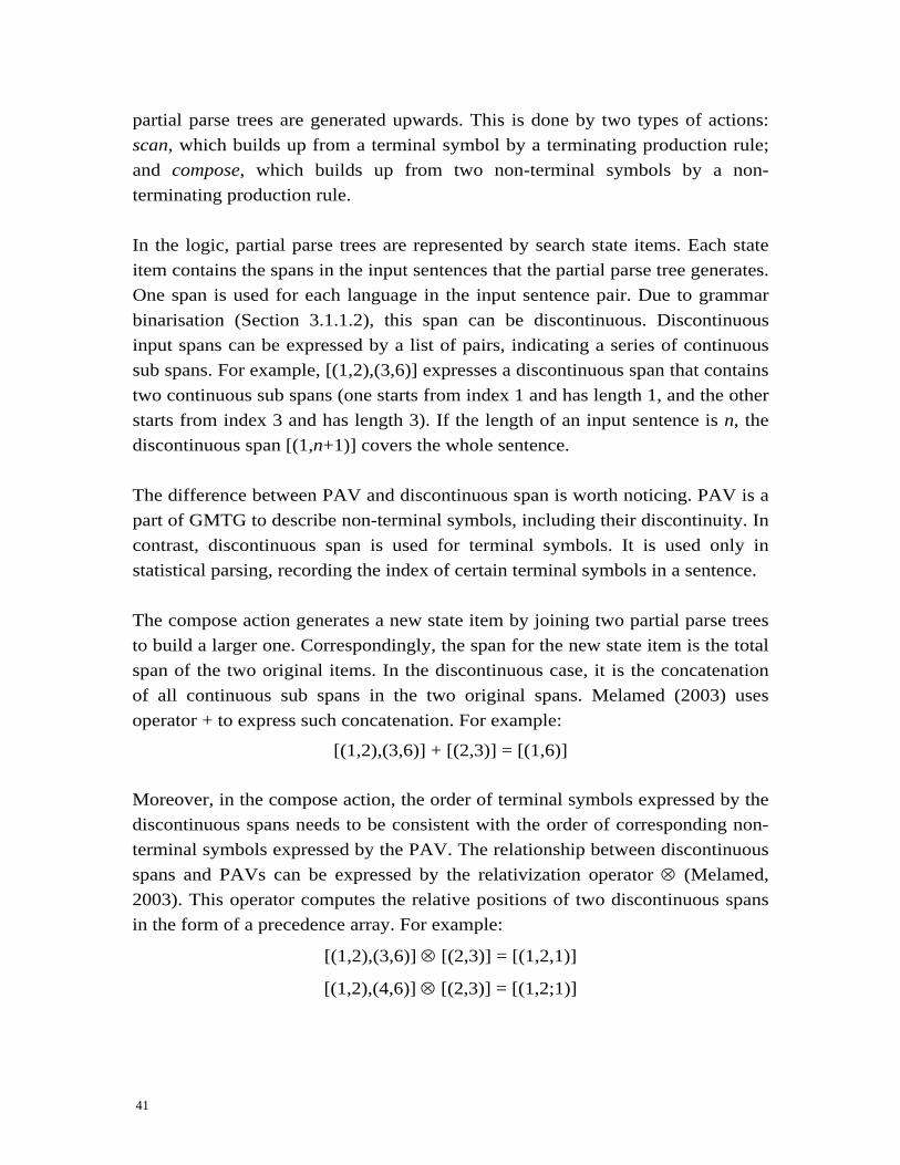
41
partial parse trees are generated upwards. This is done by two types of actions: scan, which builds up from a terminal symbol by a terminating production rule; and compose, which builds up from two non-terminal symbols by a non-terminating production rule. In the logic, partial parse trees are represented by search state items. Each state item contains the spans in the input sentences that the partial parse tree generates. One span is used for each language in the input sentence pair. Due to grammar binarisation (Section 358H3.1.1.2), this span can be discontinuous. Discontinuous input spans can be expressed by a list of pairs, indicating a series of continuous sub spans. For example, [(1,2),(3,6)] expresses a discontinuous span that contains two continuous sub spans (one starts from index 1 and has length 1, and the other starts from index 3 and has length 3). If the length of an input sentence is n, the discontinuous span [(1,n+1)] covers the whole sentence. The difference between PAV and discontinuous span is worth noticing. PAV is a part of GMTG to describe non-terminal symbols, including their discontinuity. In contrast, discontinuous span is used for terminal symbols. It is used only in statistical parsing, recording the index of certain terminal symbols in a sentence. The compose action generates a new state item by joining two partial parse trees to build a larger one. Correspondingly, the span for the new state item is the total span of the two original items. In the discontinuous case, it is the concatenation of all continuous sub spans in the two original spans. Melamed (2003) uses operator + to express such concatenation. For example:
[(1,2),(3,6)] + [(2,3)] = [(1,6)] Moreover, in the compose action, the order of terminal symbols expressed by the discontinuous spans needs to be consistent with the order of corresponding non-terminal symbols expressed by the PAV. The relationship between discontinuous spans and PAVs can be expressed by the relativization operator ⊗ (Melamed, 2003). This operator computes the relative positions of two discontinuous spans in the form of a precedence array. For example:
[(1,2),(3,6)] ⊗ [(2,3)] = [(1,2,1)]
[(1,2),(4,6)] ⊗ [(2,3)] = [(1,2;1)]
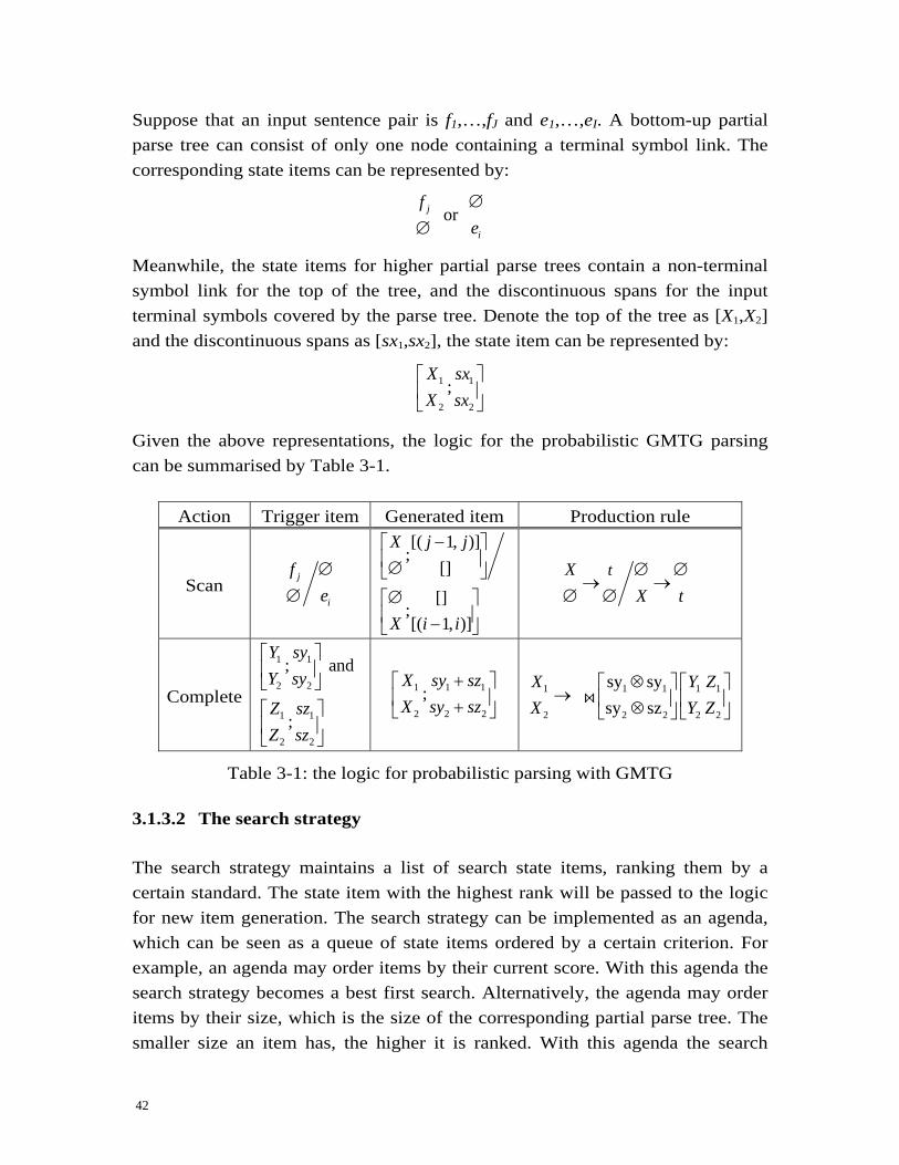
42
Suppose that an input sentence pair is f1,…,fJ and e1,…,eI. A bottom-up partial parse tree can consist of only one node containing a terminal symbol link. The corresponding state items can be represented by:
or j
i
fe∅
∅
Meanwhile, the state items for higher partial parse trees contain a non-terminal symbol link for the top of the tree, and the discontinuous spans for the input terminal symbols covered by the parse tree. Denote the top of the tree as [X1,X2] and the discontinuous spans as [sx1,sx2], the state item can be represented by:
1 1
2 2
;X sxX sx⎡ ⎤⎢ ⎥⎣ ⎦
Given the above representations, the logic for the probabilistic GMTG parsing can be summarised by 359HTable 3-1.
Action Trigger item Generated item Production rule
Scan j
i
fe∅
∅
[( 1, )];
[]
[];[( 1, )]
X j j
X i i
−⎡ ⎤⎢ ⎥∅⎣ ⎦∅⎡ ⎤⎢ ⎥−⎣ ⎦
tX
X t∅ ∅
→ →∅ ∅
Complete
1 1
2 2
1 1
2 2
; and
;
Y syY sy
Z szZ sz
⎡ ⎤⎢ ⎥⎣ ⎦⎡ ⎤⎢ ⎥⎣ ⎦
1 1 1
2 2 2
;X sy szX sy sz
+⎡ ⎤⎢ ⎥+⎣ ⎦
1 1 1 1 1
2 2 2 2 2
sy sy
sy szX Y ZX Y Z
⊗⎡ ⎤ ⎡ ⎤→ ⎢ ⎥ ⎢ ⎥⊗⎣ ⎦ ⎣ ⎦
><
Table 3-1: the logic for probabilistic parsing with GMTG 3.1.3.2 The search strategy The search strategy maintains a list of search state items, ranking them by a certain standard. The state item with the highest rank will be passed to the logic for new item generation. The search strategy can be implemented as an agenda, which can be seen as a queue of state items ordered by a certain criterion. For example, an agenda may order items by their current score. With this agenda the search strategy becomes a best first search. Alternatively, the agenda may order items by their size, which is the size of the corresponding partial parse tree. The smaller size an item has, the higher it is ranked. With this agenda the search
43
strategy becomes a bottom-up search. This experiment uses a best-first agenda. Besides best-first and bottom-up search, A-star search (Russell and Norvig, 2003) can also be used as the search strategy. The difference between A-star search and best-first search is that A-star search ranks an item not by its current score, but by an estimation of its best total score. The best total score of an item is that of the best possible complete parse tree built from the current partial parse tree, and is the combination of the current score and the estimated best score for the rest of the possible total parse tree. The advantage of A-star search is that by accurate estimation of total scores, it is possible to expand a much smaller search space before a goal is found. 3.1.3.3 The termination condition Apart from the common parsing goal that the whole input is included into a parse tree, there are other termination conditions. For example, it may be necessary to terminate the parsing process if it is taking too much time, or using up the memory resource. It is also possible to have composite termination conditions by using logical conjunctions and disjunctions. For example, a parsing goal may be a parse tree that “starts from a special non-terminal symbol AND covers the whole input span”. Or the goal may be “running for 24 hours OR using more than 4GB memory”. 3.1.4 The training process The last two sections introduced the model and the decoding process for the statistical parsing of GMTG. The other important factor is the learning process, where parameters in the statistical model (i.e. probabilities for production rules) are determined. In the mono-lingual case (Section 2.3.2), two different learning methods are used to train PCFG, making use of different forms of corpora. Similarly, the following training methods can be used for bilingual GMTG. 3.1.4.1 Maximum likelihood training Maximum likelihood estimation can be used when a manually parsed treebank is available (Section 2.3.2). For the training of statistical GMTG, such a treebank enabling maximum likelihood learning must contain manually parsed sentence pairs in GMTG.
44
Currently there is no existing bilingual GMTG treebank that contains enough parsed sentence pairs to be used in this experiment. However, parallel sentences in Chinese and English are available in reasonable size. What is more, the monolingual structure for both Chinese and English can be derived from existing statistical parsers. Therefore, by combining corresponding monolingual parse trees, it is possible to introduce a bilingual treebank. Such a process is called hierarchical alignment (Melamed and Wang, 2005). Hierarchical alignment is currently a necessary step to train probabilistic GMTG. After this step, maximum likelihood learning can be performed from the output bilingual treebank. Section 362H3.2 will show that hierarchical alignment can be done by the generalised parsing process. 3.1.4.2 Expectation maximisation training As was described in Section 363H2.3.2, the EM machine learning algorithm can be used to train a probabilistic grammar without a treebank. For statistical GMTG, the training data can be a set of parallel sentence pairs which can be generated by GMTG. Starting with an initial probabilistic grammar, the algorithm updates it by EM iterations over the training sentence pairs. This method converges to a grammar that brings the probability of the training data to a local maximum value. However, the effect of EM training is dependent on the initial values. When the initial grammar is not well chosen, the local maximum value can be far from the global maximum value. Because of this, the EM training method is too unreliable to be used alone for GMTG training. At the same time, it can be used to further improve an initial grammar that is reasonably near the global optimal value. For example, it can be used for an optimisation after maximum likelihood learning.
3.2 Hierarchical alignment by parsing The goal of hierarchical alignment is building a bilingual treebank from two mono-lingual treebanks. For each pair of mono-lingual tree, the corresponding symbols are aligned hierarchically to make a combined bilingual tree. In order to achieve this goal, the algorithmic solution is searching for the best aligned bingual tree from all possible alignments.

45
Without introducing any restrictions, two mono-lingual trees can be combined arbitrarily – one symbol in a mono-lingual tree can be aligned to any symbol in the other. Each possible combination makes a candidate for the bilingual parse tree. Correspondingly, the set of all such combinations makes a search space. In order to find the correctly combined bilingual tree from this search space, we can score each candidate combination, enabling the search goal to get the best score. This search problem looks like statistical parsing in that it is to find the bilingual tree that has the highest score among many bilingual trees. The difference is that the arbitrarily aligned candidate trees can be not in GMTG at all. In spite of this, we can still borrow experience from the statistical model which calculates the score of a parse tree. As was described in Section 364H2.3.2 and Section 365H3.1.2, the score of a parse tree can be seen as the overall score of the production rules that generate it. In this way the calculation of parse tree scores is reduced to the calculation of production scores, which has simpler forms. Candidates for hierarchical alignment can be scored in the same way, treating each combined tree as if it were generated by “production rules”. The score of these pseudo production rules can be calculated by the component mono-lingual grammars. The next two sections describe two methods to score these pseudo production rules, with different information from the mono-lingual grammars. 3.2.1 Calculating combined pseudo production rules from one
mono-lingual grammar This section describes the calculation of combined pseudo production rules by only one mono-lingual grammar, which is comparatively simpler. Suppose that the first language is used. In this case, all non-terminal symbols in the second language can be represented by a dummy non-terminal symbol NULL. In the GCNF format (Section 366H3.1.1.3), there are two kinds of production rules – the terminating production rules and the non-terminating production rules. A terminating production rule contains only one link on the right hand side. In the lexicalised form, it can be written as:
1 1 1
2 2 2
[ ] or
[ ]X h h
LHS RHSX h h∅ ∅
→ = → →∅ ∅
(3-3)
46
In Equation 3-3, Xd[hd] represents a non-terminal symbol Xd whose head word is hd. For the terminating production rules, only one language is active (As indicated by Equation 3-3, the inactive language has empty symbol ∅ on both sides of the production rule; see also Section 367H3.1.1.3). Correspondingly, the scores of combined pseudo production rules are decided by the active language. Therefore, when the first language is active, P(RHS|LHS)=P(h1|X1[h1]) – the probability is the same as the corresponding mono-lingual production score. Similarly, when the second language is active, P(RHS|LHS)=P(h2|X2[h2]). However, because only the first language is used in this method, we have P(h2|X2[h2])=1 only when X2=NULL, and P(h2|X2[h2])=0 otherwise. A non-terminating production rule consists of a PAV and a symbol vector on the right hand side. A lexicalised non-terminating production rule can be written as:
1 1 1 1 1 1 1
2 2 2 2 2 2 2
[ ] [ ] [ ]
[ ] [ ] [ ]X h pa Y g Z h
LHS RHSX h pa Y g Z h
⎡ ⎤ ⎡ ⎤→ = → ⎢ ⎥ ⎢ ⎥
⎣ ⎦ ⎣ ⎦>< (3-4)
In the above equation, Xd, Yd and Zd are non-terminal symbols, hd and gd are head words and pad are precedence arrays. Therefore, P(RHS|LHS) can be written as
1 2 1 2 1 2 1 2 1 2 1 2( , , , , , , , | , , , )P pa pa Y Y Z Z g g X X h h . Using the chain rule, this probability can be broken down as follows:
1 2 1 2 1 2 1 2 1 2 1 2( , , , , , , , | , , , )P pa pa Y Y Z Z g g X X h h = 1 1 1 1 1 2 1 2( , , , | , , , )P pa g Y Z X X h h × 2 2 1 1 1 1 1 2 1 2( , | , , , , , , , )P Y Z pa g Y Z X X h h × 2 1 1 1 2 1 2 1 2 1 2( | , , , , , , , , , )P g pa g Y Y Z Z X X h h × 2 1 1 2 1 2 1 2 1 2 1 2( | , , , , , , , , , , )P pa pa g g Y Y Z Z X X h h (3-5) To further simplify the calculation of Equation 368H3-5, the following independence assumptions can be made:
(1) 1 1 1 1 1 2 1 2 1 1 1 1 1 1( , , , | , , , ) ( , , , | , )P pa g Y Z X X h h P pa g Y Z X h= (mono-lingual production)
(2) 2 22 2 1 1 1 1 1 2 1 2
1 if ( , | , , , , , , , )
0 otherwise Y Z NULL
P Y Z pa g Y Z X X h h= =⎧
= ⎨⎩
(the unused language)
(3) 2 1 1 1 2 1 2 1 2 1 2 2 1( | , , , , , , , , , ) ( | )P g pa g Y Y Z Z X X h h P g g= (word-to-word probability)
(4) 2 1 1 2 1 2 1 2 1 2 1 2 21( | , , , , , , , , , , ) ( )( )
P pa pa g g Y Y Z Z X X h h P pafμ
= = , where ( )fμ is the
number of unique precedence arrays of the maximum fanout f.
47
Thus the simplified calculation for the pseudo non-terminating production rules is as follows:
1 1 1 1 1 1 2 12 2
( , , , | , ) ( | ) , if and are both ( )( | )
0 , otherwise
P pa g Y Z X h P g g Y Z NULLfP RHS LHS μ
⎧⎪= ⎨⎪⎩
(3-6)
3.2.2 Calculating combined pseudo production scores from two
mono-lingual grammars Moving from the simpler case, this section describes the calculation of combined pseudo production rules from both mono-lingual grammars. Similar to Section 369H3.2.1, the scores for combined pseudo terminating production rules are calculated by the active language. When the first language is active, P(RHS|LHS)=P(h1|X1[h1]), and this probability is the same as the corresponding mono-lingual production rule. Similarly, when the second language is active, P(RHS|LHS)=P(h2|X2[h2]), and this probability is the corresponding mono-lingual production score of the second language. For combined non-terminating production rules, the calculation can be based on Equation 370H3-6. In a simple form, the production score of the second language can be incorporated into the combined production score as a factor. In equation form:
( | )P RHS LHS = 1 2 1 2 1 2 1 2 1 2 1 2( , , , , , , , | , , , )P pa pa Y Y Z Z g g X X h h
= 1 1 1 1 1 1 2 2 2 2 2 2 2 1( , , , | , ) ( , , , | , ) ( | )( )
P pa g Y Z X h P pa g Y Z X h P g gfμ
3.2.3 Hierarchical alignment by generalised parsing Section 371H3.2.1 and Section 372H3.2.2 define possible ways to calculate the combined production scores. From these production scores, the score of combined bilingual trees can be calculated, and the best tree can be chosen by the search algorithm. In summary, the input for the hierarchical alignment problem is a set of aligned bilingual sentences, the output is a bilingual parse tree, and the search process is based on the calculation of candidate trees by production scores. All the above conditions are the same as the bilingual parsing problem, enabling hierarchical

48
alignment to be implemented by generalised parsing. Among the five generalised parsing components, the semiring of hierarchical alignment is the same as that of bilingual parsing (Section 373H3.1.3) – both are non-negative floating point numbers as probabilities. However, the grammar for hierarchical alignment is different from the grammar for bilingual parsing (i.e. probabilistic GMTG). In fact, the hierarchical alignment process is not based on any bilingual grammar – as stated in the beginning of Section 374H3.2, the candidate trees are arbitrarily combined. However, because scores are assigned to the pseudo bilingual production rules, it can be regarded as using a pseudo grammar. This pseudo grammar does not contain any production rules, but with an input symbol, it can generate possible production rules and assign scores to them, as described in Section 375H3.2.1 and Section 376H3.2.2. The external behaviour of the pseudo grammar can be made exactly the same as probabilistic GMTG, so that hierarchical alignment can use the same logic and search strategy as bilingual parsing (Section 377H3.1.3.1 and Section 378H3.1.3.2). What is more, because the parsing goals of the two problems are the same, hierarchical alignment can also use the terminating conditions in Section 379H3.1.3.3.
3.3 Translation by bilingual parsing This section describes the algorithm of SMT by GMTG parsing, using the generalised parsing algorithm. As introduced in Section 380H1.1.4, the process of SMT by parsing is a parsing process, which derives a bilingual parse tree. Given a probabilistic GMTG model, the main differences between the SMT by parsing algorithm and the GMTG parsing algorithm in Section 381H3.1.3 include: (1) the inputs for translation are mono-lingual sentences instead of bilingual sentence pairs; (2) translation sentence pairs need to be extracted from the output parse trees. It is possible to implement the decoding process of translation by generalised parsing. Comparing the five generalised parsing components, translation by parsing has the same grammar (probabilistic GMTG) and semiring (non-negative floating point numbers) as bilingual parsing. Not considering the flattening of parse trees, the termination condition and parsing goals are also the same.

49
The logic for translation needs to be different from the one for bilingual parsing (Section 382H3.1.3.1). This is mainly because the input for translation contains only one language. During the translation by parsing process, terminal symbols of the target language are not available from input. In order to build bilingual GMTG parse trees, a special action is needed to bring terminal symbols of the other language into search state items. One possible choice is the load action (Melamed and Wang, 2005), which is similar to the scan action in that it generates new items according to terminating productions. However, the load action does not take any inputs. Instead of matching input terminal symbols with terminating productions, it allows state items to be generated from any terminal symbols. Using a similar format as 383HTable 3-1, 384HTable 3-2 illustrates the logic for translation.
Action Trigger item Generated item Production rule
Scan jf∅
[( 1, )]
;X j j−⎡ ⎤⎢ ⎥∅⎣ ⎦
tX
→∅ ∅
Load None []
;X∅⎡ ⎤⎢ ⎥⎣ ⎦
X t∅ ∅→
Complete
1 1
2
1 1
2
; and
;
Y syY
Z szZ
⎡ ⎤⎢ ⎥⎣ ⎦⎡ ⎤⎢ ⎥⎣ ⎦
1 1 1
2
;X sy szX
+⎡ ⎤⎢ ⎥⎣ ⎦
1 1 1 1 1
2 2 2 2
sy sy
X Y ZX pa Y Z
⊗⎡ ⎤ ⎡ ⎤→ ⎢ ⎥ ⎢ ⎥
⎣ ⎦ ⎣ ⎦><
Table 3-2: the logic for translation by parsing It can be seen from the table that items in the translation target language do not contain any span information. This is because no input sentences in the language are available. As a consequence, there is no need to choose production rules that match the discontinuous spans in this language. pa2 in the production rule of the “complete” action denotes any precedence array in that dimension. The main differences between the translation logic and the bilingual parsing logic are the load action and the span information for the translation target language. Besides these differences, the logics for the two problems are the same. For the translation case, although all possible terminal symbols for one language are loaded, the search process will finally determine the best parse tree and remove
50
the unlikely items by scores. A disadvantage of the load action is that a considerable number of items are introduced into the search space, which will impact decoding efficiency. A possible improvement for the load action is to generate items only from those terminal symbols that are possible translations of the terminal symbols from the source sentence. This will reduce the search space considerably, because the possible word translations for an input sentence are much fewer than all the words from the vocabulary. Finally, corresponding to the above logic definition, translation by parsing can also use the same search strategy as bilingual parsing, such as the best-first agenda approach.
51
Chapter 4
The details of experiments
4.1 Introduction The above theory is applied to Chinese-English SMT by this thesis with large-scale experiments. This chapter records the details of the experiments, including the software systems, the training and testing corpora, and the typical process that is used by all the experiments of this thesis. The output and research questions are discussed in 385HChapter 5. The system for the experiments is built upon existing pieces of software. The engineering work includes the choosing and compiling of the software systems and libraries, the selecting and formatting of corpora, the code analysis in accordance with the theory of the last two chapters, the software development work to combine and coordinate different software systems, and the application of automatic MT evaluation methods. One of the challenges of the experiments is training the system with significantly large amounts of data within a reasonable time frame; the techniques used include filtering dispensable time consuming data, running tasks in parallel, and doing experiments incrementally. 4.2 Software 4.2.1 GenPar – the software framework for generalised parsing GenPar (Burbank et al., 2005) is the major software framework used by the experiments. It provides an implementation of the generalised parsing algorithm. GenPar is written in C++. It was developed during the 2005 Johns Hopkins Language and Speech Processing Workshop.
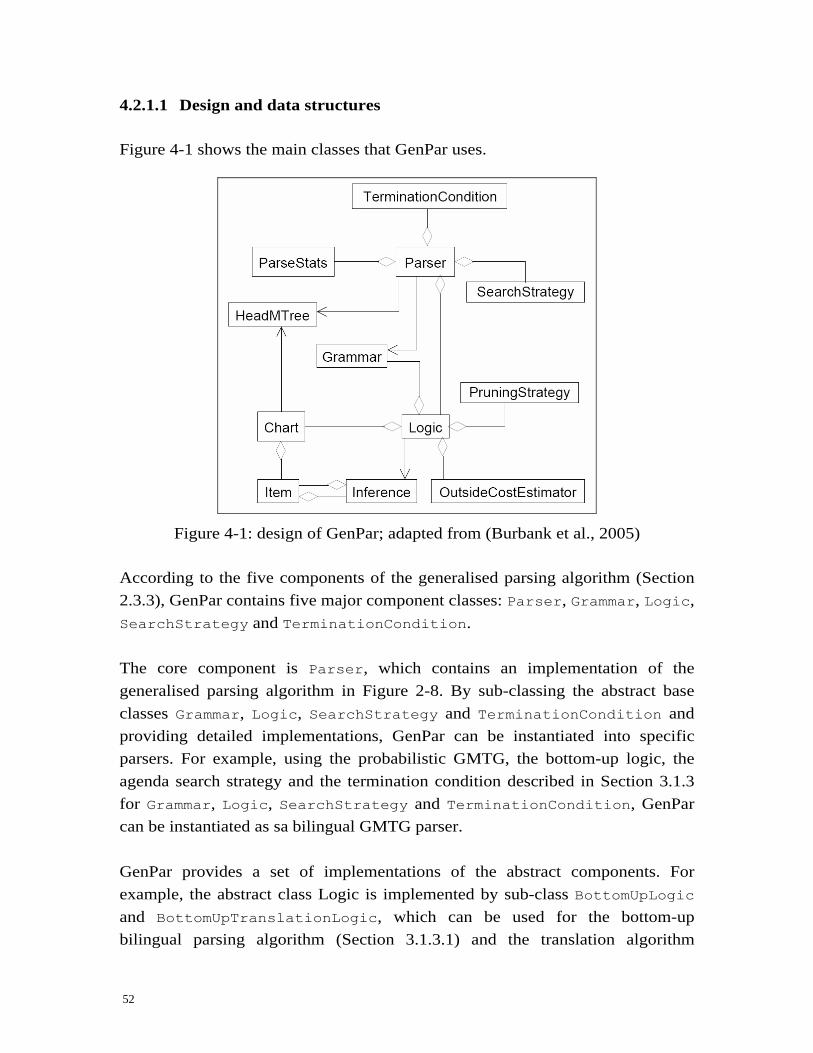
52
4.2.1.1 Design and data structures Figure 4-1 shows the main classes that GenPar uses.
Figure 4-1: design of GenPar; adapted from (Burbank et al., 2005)
According to the five components of the generalised parsing algorithm (Section 2.3.3), GenPar contains five major component classes: Parser, Grammar, Logic, SearchStrategy and TerminationCondition. The core component is Parser, which contains an implementation of the generalised parsing algorithm in Figure 2-8. By sub-classing the abstract base classes Grammar, Logic, SearchStrategy and TerminationCondition and providing detailed implementations, GenPar can be instantiated into specific parsers. For example, using the probabilistic GMTG, the bottom-up logic, the agenda search strategy and the termination condition described in Section 3.1.3 for Grammar, Logic, SearchStrategy and TerminationCondition, GenPar can be instantiated as sa bilingual GMTG parser. GenPar provides a set of implementations of the abstract components. For example, the abstract class Logic is implemented by sub-class BottomUpLogic and BottomUpTranslationLogic, which can be used for the bottom-up bilingual parsing algorithm (Section 3.1.3.1) and the translation algorithm
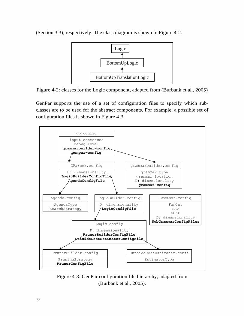
53
(Section 3.3), respectively. The class diagram is shown in Figure 4-2.
Figure 4-2: classes for the Logic component, adapted from (Burbank et al., 2005) GenPar supports the use of a set of configuration files to specify which sub-classes are to be used for the abstract components. For example, a possible set of configuration files is shown in Figure 4-3.
Figure 4-3: GenPar configuration file hierarchy, adapted from
(Burbank et al., 2005).
Logic
BottomUpLogic
BottomUpTranslationLogic
gp.config
input sentences debug level
grammarbuilder-configgenpar-config
grammarbuilder.config
grammar type grammar location D: dimensionality grammar-config
GParser.config
D: dimensionality LogicBuilderConfigFile
AgendaConfigFile
Agenda.config
AgendaType SearchStrategy
LogicBuilder.config
D: dimensionality LogicConfigFile
Grammar.config
FanOut PAV GCNF
D: dimensionality SubGrammarConfigFiles
Logic.config
D: dimensionality PrunerBuilderConfigFile
OutsideCostEstimatorConfigFile
PrunerBuilder.config
PruningStrategy PrunerConfigFile
OutsideCostEstimater.confi
EstimatorType
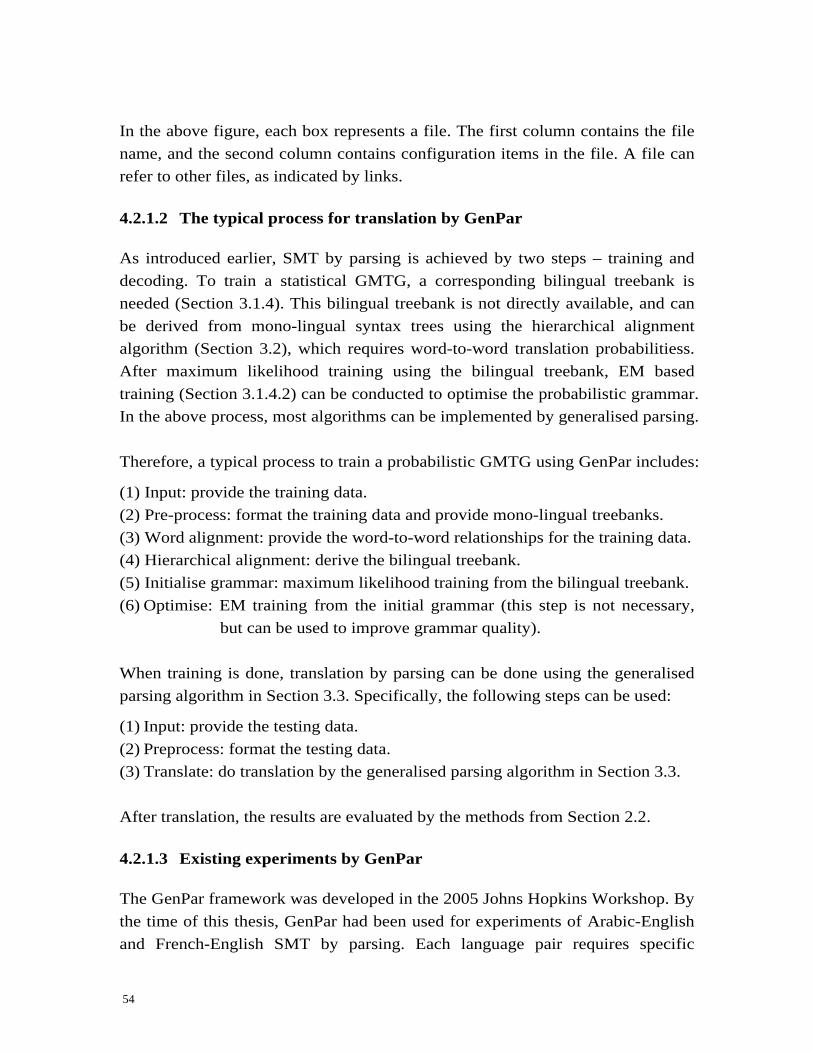
54
In the above figure, each box represents a file. The first column contains the file name, and the second column contains configuration items in the file. A file can refer to other files, as indicated by links. 4.2.1.2 The typical process for translation by GenPar As introduced earlier, SMT by parsing is achieved by two steps – training and decoding. To train a statistical GMTG, a corresponding bilingual treebank is needed (Section 3.1.4). This bilingual treebank is not directly available, and can be derived from mono-lingual syntax trees using the hierarchical alignment algorithm (Section 3.2), which requires word-to-word translation probabilitiess. After maximum likelihood training using the bilingual treebank, EM based training (Section 3.1.4.2) can be conducted to optimise the probabilistic grammar. In the above process, most algorithms can be implemented by generalised parsing. Therefore, a typical process to train a probabilistic GMTG using GenPar includes:
(1) Input: provide the training data. (2) Pre-process: format the training data and provide mono-lingual treebanks. (3) Word alignment: provide the word-to-word relationships for the training data. (4) Hierarchical alignment: derive the bilingual treebank. (5) Initialise grammar: maximum likelihood training from the bilingual treebank. (6) Optimise: EM training from the initial grammar (this step is not necessary,
but can be used to improve grammar quality). When training is done, translation by parsing can be done using the generalised parsing algorithm in Section 3.3. Specifically, the following steps can be used:
(1) Input: provide the testing data. (2) Preprocess: format the testing data. (3) Translate: do translation by the generalised parsing algorithm in Section 3.3. After translation, the results are evaluated by the methods from Section 2.2. 4.2.1.3 Existing experiments by GenPar The GenPar framework was developed in the 2005 Johns Hopkins Workshop. By the time of this thesis, GenPar had been used for experiments of Arabic-English and French-English SMT by parsing. Each language pair requires specific
55
processing, and the overall French-English translation was more accurate than the Arabic-English translation (Burbank et al., 2005). In Section 5.1.1.3, the Chinese-English SMT by parsing results of this thesis are compared with the results of existing Arabic-English and French-English experiments with GenPar. 4.2.2 The Bikel statistical (mono-lingual) parser The Bikel parser (Bikel, 2002) is a mono-lingual parser that supports different types of statistical parsing models. It is used in the experiments to produce English and Chinese mono-lingual grammars. This parser is implemented in Java. The Bikel parser requires the part-of-speech information for each word in the input sentence. Therefore, before using the parser, POS tagging (Jurafsky and Martin, 2000) is required, which assigns POS tags to the input words. 4.2.3 The LingPipe libraries for the Chinese segmentation task The LingPipe natural language processing library is used by this thesis for Chinese word segmentation (Section 1.1.5). It is chosen because of its comparatively high accuracy. LingPipe uses an n-gram based language model. It does Chinese word segmentation by a spelling correction algorithm. The library is written in Java. 4.2.4 The Stanford statistical tagger The Stanford Tagger (Toutanova and Manning, 2000) is used by this thesis for the POS tagging of both Chinese and English. It is based on the maximum entropy probabilistic model (Ratnarparkhi, 1997). An advantage of this model is that it allows different features to be selected in the calculation of tagging probability. The Stanford Tagger is written in Java. 4.2.5 GIZA++ – the word alignment tool GIZA++ (Och and Ney, 2000) is a general word alignment tool. It is used by this thesis to obtain word-to-word translation probabilities between Chinese and English. It is based on the word alignment models in Section 2.1.2, and it incorporates many features. GIZA++ is written in C++.

56
4.3 Training and testing data 4.3.1 Training data Hong Kong Parallel Text corpus is used for the bilingual training. It is produced by the Linguistic Data Consortium (LDC). Its catalog number is LDC2004T08 and it has ISBN 1-58563-290-2. The corpus contains parallel articles in Chinese and English, together with specifications of the (many-to-many) sentence alignment in each pair of articles. There are three collections in the corpus, containing 59 million Chinese words and 49 million English words. Only the News collection is used for this thesis, which contains 27 million Chinese words and 15 million English words (in 2,681 thousand Chinese sentences and 2,952 thousand English sentences, respectively). The Chinese Treebank version 4.0 is used as the Chinese mono-lingual grammar treebank. It is produced by LDC. Its catalog number is LDC2004T05 and it has ISBN 1-58563-287-2. The corpus contains a collection of Chinese articles, in which each sentence is manually segmented, POS tagged and annotated with a CFG parse tree. There are 664,633 characters (in 15,162 sentences) in the corpus. The English Treebank version 3.0 is used as the English mono-lingual grammar treebank. It is produced by LDC. Its catalog number is LDC99T42 and it has ISBN 1-58563-163-9. The corpus contains a collection of English articles, from which each sentence is manually POS tagged and parsed. The whole corpus contains over a million words, while this thesis uses only the Wall Street Journal (WSJ) sub collection. Three corpora provided by the first International Chinese Word Segmentation Bakeoff (from Academia Sinica, Hong Kong City University and Beijing University) are used for the Chinese segmentation task. These corpora contain segmented Chinese sentences. There are in total over 7 million words in the corpora. 4.3.2 Testing data The Hong Kong Parallel Text corpus is used for part of the testing data. Parallel sentences in the corpus that are not used for training are extracted for testing.
57
The Multiple-Translation Chinese (MTC) Part 3 corpus is used for another part of the testing data. It was produced by LDC. Its catalog number is LDC2004T07 and it has ISBN 1-58563-289-9. The corpus contains 100 Chinese articles, each having four independent English translations. The corpus is sentence-aligned, and there are 935 Chinese sentences in total. 4.4 Details for a typical experiment Following the process of Section 403H4.2.1.2, this section records the detailed process of a typical experiment, including 6 steps for training, 3 steps for translation and 1 step for evaluation. This process is used by most of the experiments. 4.4.1 Input for training This section describes the details of training step (1) given in Section 404H4.2.1.2. Two files are produced in this step (L1.text and L2.text), each containing the training sentences in Chinese and English, respectively. The nth sentence in one file is the corresponding translation of the nth sentence in the other. The source files for this step are the Hong Kong Parallel Text data, which are formatted in loose XML, and separated into three folders containing Chinese text, English text and alignment information. A Python script (corpus_rfmt.py) is made to extract the corpus data and format them for output. During the process, we made two simplifications: (1) When there are sentences that are not in one-to-one relationship (e.g. one English sentence corresponds to multiple Chinese sentences), they are discarded. (2) When there are quotations (i.e. there are Chinese quotations in the English version), they are discarded from both sides. Because the Kong Hong Parallel Text is in traditional Chinese (BIG5 encoded), it is first translated into simplified Chinese (GB2312 encoded) so that it can be used consistently with the Chinese Treebank. The translation is table-based3F
1, because the two character sets are almost many-to-one related. After this, all brackets (“(”, “)”) are converted to the Chinese version (GB-2312 encoded). This is to avoid clashing with the Stanford tagger, which uses brackets to hold tag information. 1 See http://freshmeat.net/projects/autoconvert/ for more details.
58
4.4.2 Pre-processing for training This section describes the details of training step (2) in Section 4.2.1.2. The input files of this step are the input texts from Section 4.4.1 (L1.text and L2.text). The productions of this step include two mono-lingual treebanks (L1.tb and L2.tb), two files containing segmented input Chinese text and tokenised input English text (L1.tok.text and L2.prep.text), as well as formatted files containing tokenised text (output.snt and output.snt). This step also produces interim outputs, such as tagged Chinese and English sentences. 4.4.2.1 Mono-lingual treebanks The Bikel parser is used to produce mono-lingual treebanks for both Chinese and English. It is trained with the Chinese Treebank 4 and the English Treebank 3, respectively. Before training, the files from the Chinese Treebank are switched from “fid” format to “mrg” format for the parser. This is done by making a Python script (fid2mrg.py). After training, the output models are saved into ctb.obj.gz (Chinese) and etb.obj.gz (English). With the trained models, the Bikel parser can be used for mono-lingual parsing. Because the Bikel parser requires input sentence with POS information, both the Chinese (L1.text) and the English (L2.text) sentences need to be POS-tagged. Besides, the input Chinese sentences also need to be segmented. LingPipe is used for Chinese segmentation. Three corpora provided by the first International Chinese Word Segmentation Bakeoff teams (i.e. Academia Sinica, Hong Kong City University and Beijing University) are converted into simplified Chinese (GB2312 encoded), merged into one file, and then used to train the segmentor. The Chinese sentences in L1.text are segmented and saved into L1.tok.text. English sentences do not need segmentation. However, they also need tokenisation (e.g. separating punctuation marks from words by space). This task is also performed by the Stanford tagger, and processed together with POS tagging. The tokenised English sentences are saved as L2.prep.text. Both Chinese and English are tagged using the Stanford statistical tagger. The tagger is trained with tagged corpora from the Chinese Treebank 4 and the English Treebank 3, respectively. Before training, corpus data for each language are merged into one file, and transferred into the Stanford tagger file format. This
59
is done by making two Python scripts (cn_tag_form.py and en_tag_form.py). After training the tagger, we prepare the segmented Chinese file (L1.tok.text) and the input English file (L2.text) for tagging. For example, the newest version of the Stanford tagger supports Chinese by Unicode characters. However, the input Chinese text is encoded in GB-2312. Thus the input text (L1.tok.text) is first switched to Unicode (by making gb2utf.py), and then the tagged text is switched back to GB-2312 (by making utf2gb.py). After tagging, the output tagged Chinese and English sentences are saved into L1.tagged.text and L2.tagged.text, respectively. The tagged sentences are passed to the Bikel parser, which has just been trained. The output for the parser needs to be configured so that it will include lexical head information, which is necessary for the hierarchical alignment process. The following line is added to the parser’s setting file:
parser.decoder.outputHeadLexicalizedLabels=true The above configuration is required for both Chinese and English parsing. For English parsing, an alternative choice is using the GenPar add-on setting file ws05Collins.properties instead of the default collins.properties file. The parsing process requires significant computational resource. For the aim of producing novel result for Chinese-English translation by parsing, the training data set is expected to be as large as possible. In order to derive parsed data within the time frame for this thesis, the tagged data are divided into 32 groups and processed on 32 separate machines, including jet1 and jet2, as well as booth3 – booth32 in the Thom building. Parsing output files are then merged into one file (L1.text.tb for Chinese and L2.text.tb for English). Furthermore, earlier parsing outputs are used for translation experiments immediately, before all tagged sentences are parsed. In general, the GenPar translation experiments were performed with smaller training data simultaneously as larger training data was being prepared. It took around 2 months for all the sentences to be parsed. After parsing, mono-lingual treebanks are extracted from the output parse trees for hierarchical alignment. In each experiment, a specific number of parse trees are extracted from the parser’s output (by making extract_trees.py). During this process, the parse trees are filtered and unhelpful data are discarded. For example, when the Bikel’s parser fails to parse a sentence, it produces “null” as
60
the output. These null parse trees in either Chinese or English are removed, together with their corresponding translation. Also, to improve time and space efficiency, sentences that are longer than 30 words are filtered out. Such sentences are comparatively few, and testing shows that the GenPar framework is exponentially inefficient with such sentences during hierarchical alignment. Before the extracted parse trees are used by GenPar, the terminal symbols are replaced by integers, so that the generalised parsing process is more efficient. This is done by a Perl script (integerize_trees) provided by GenPar. The final Chinese and English parse trees are saved to L1.tb and L2.tb, respectively. 4.4.2.2 Formatted sentence pairs and mono-lingual sentences For the use in the next steps, segmented Chinese sentences and tokenised English sentences are grouped into one file, where each Chinese sentence is paired with the corresponding English translation by <s> and </s> tags. This is achieved by making a Python script (weavefiles.py), which reads sentences from multiple files and groups corresponding lines by <s> and </s> tags. The input files for this script are the segmented Chinese text (L1.tok.text) and tokenised English text (L2.prep.text) from Section 4.4.2.1, and the output file is called output.snt. weavefiles.py is also applied to Chinese mono-lingual sentences, and the output texts are saved at output.snt.1D. 4.4.3 Word alignment This section describes the details of training step (3) in Section 4.2.1.2. The input files for this step are L1.tok.text and L2.prep.text from Section 4.4.2. This step produces a word-to-word alignment model file (links). This step is based on the theory of Section 2.1.2. GIZA++ is used to derive word-to-word alignments. The detailed steps are shown as follows:
(1) Run plain2snt.output (which is compiled together with the GIZA++ package) on L1.tok.text and L2.prep.text, and get the following output files:
L1.tok.text.vcb (vocabulary file for Chinese)
61
L2.prep.text.vcb (vocabulary file for English) L1.tok.text_L2.prep.text.snt (integerised sentence alignment file)
This step replaces words with integers for both Chinese and English, so that they will be processed more efficiently.
(2) Run mkcls (which is a separate package from GIZA++) on L1.tok.text and L2.prep.text and generate word classes L1.tok.text.vcb.classes (for Chinese) and L2.prep.text.vcb.classes (for English).
This step is optional. It does bilingual word classification (i.e. group words into equivalent classes – not studied in this thesis; Och, 1999).
(3) Run GIZA++: GIZA++ -S L2.prep.text.vcb -T L1.tok.text.vcb \
-C L2.prep.text_L1.tok.text.snt –o L1toL2
The output file L1toL2.A3.final contains the word-to-word probabilities ( | )P f e (Section 411H2.1.2), where e represents an English word and f represents a
Chinese word. After the above process, the output of GIZA++ is turned into the file format that GenPar can use. This is done by a Perl script provided by GenPar (giza2ww). This thesis also adapts a bi-directional alignment method, which was used by existing Arabic-English and French-English translations by GenPar (Burbank et al., 2005). This process includes the following steps:
(1) Use GIZA++ to generate alignment in both Chinese-English and English-Chinese direction.
(2) Take the intersection of alignments for each sentence in step (1) as the training set for the output alignment.
(3) Using the maximum likelihood estimation, calculate the joint-alignment probability as:
,
( , )( , )
( , )x y
i ji j
x yc e
Count c eP c e
Count c e=∑
In the above equation, ci and ej are a Chinese word and an English word that are aligned together, while cx represents any Chinese word in the training set and ey represents any English word in the training set.
(4) Use all word pairs that have non-zero probability from step (3) as the word
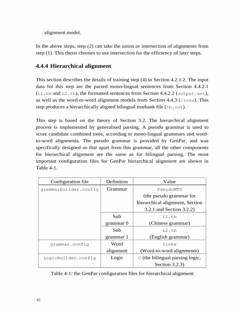
62
alignment model. In the above steps, step (2) can take the union or intersection of alignments from step (1). This thesis chooses to use intersection for the efficiency of later steps. 4.4.4 Hierarchical alignment This section describes the details of training step (4) in Section 4.2.1.2. The input data for this step are the parsed mono-lingual sentences from Section 4.4.2.1 (L1.tb and L2.tb), the formatted sentences from Section 4.4.2.2 (output.snt), as well as the word-to-word alignment models from Section 4.4.3 (links). This step produces a hierarchically aligned bilingual treebank file (tb.out). This step is based on the theory of Section 3.2. The hierarchical alignment process is implemented by generalised parsing. A pseudo grammar is used to score candidate combined trees, according to mono-lingual grammars and word-to-word alignments. The pseudo grammar is provided by GenPar, and was specifically designed so that apart from this grammar, all the other components for hierarchical alignment are the same as for bilingual parsing. The most important configuration files for GenPar hierarchical alignment are shown in Table 4-1.
Configuration file Definition Value Grammar PseudoMTG
(the pseudo grammar for hierarchical alignment, Section
3.2.1 and Section 3.2.2) Sub
grammar 0 L1.tb
(Chinese grammar)
grammarbuilder.config
Sub grammar 1
L2.tb
(English grammar) grammar.config Word
alignment links
(Word-to-word alignments) LogicBuilder.config Logic C (the bilingual parsing logic,
Section 3.2.3)
Table 4-1: the GenPar configuration files for hierarchical alignment

63
4.4.5 Initialise grammar This section describes the details of training step (5) in Section 4.2.1.2. The input files for this step are the formatted sentence pairs from Section 4.4.2 (output.snt) and the bilingual treebank from Section 4.4.4 (tb.out). This step produces a probabilistic grammar model (pmtg.mle). This step is based on the theory of Section 3.1.4.1. Bilingual trees from tb.out are scanned, and the production probabilities are estimated by the maximum likelihood principle. This step is achieved using the GenPar program trees2grammar. 4.4.6 Optimise This section describes the details of training step (6) in Section 4.2.1.2. The input files for this step are the formatted sentence pairs from Section 4.4.2 (output.snt) and the initialised grammar from Section 4.4.5 (pmtg.mle). This step produces the optimised probabilistic grammar model (model_final). This step is based on the theory from Section 3.1.4.2. The output grammar from the last step is taken as the initial value, and several EM iterations are taken to update the grammar to a local optimal value. This step is achieved using the GenPar program treeLearn. 4.4.7 Input for translation This section describes the details of translation step (1) in Section 4.2.1.2. Two files are produced in this step (L1.text and L2.text), each containing testing sentences in Chinese and English, respectively. The nth sentence in one file is the corresponding translation of the nth sentence in the other. L1.text and L2.text make a testing set, where L1.text is the source text for translation and L2.text is the reference translation. Two testing sets are prepared using separate corpora. Firstly, parallel sentences from Hong Kong Parallel Text that are not used as training data are extracted as a test set. This is done by making a Python script (make_test_data.py). 983 sentence pairs are
64
extracted as the testing data. Secondly, in order to test different writing styles, Multiple-Translation Chinese (MTC) Part 3 is used as another test set. There are in all 935 sentences in this corpus, which is comparable to the first test set. 4.4.8 Pre-process for translation This section describes the details of translation step (2) in Section 4.2.1.2. The input files of this step are the testing text from Section 4.4.7 (L1.text and L2.text). The productions of this step include two files containing segmented input Chinese text and tokenised input English text (L1.prep.text and L2.prep.text), as well as two formatted files containing the tokenised text (output.snt and output.snt.1D). Similar to Section 4.4.2, LingPipe libraries are used for Chinese segmentation. The library has been trained previously. L1.text is segmented and saved as L1.prep.text. L2.text is tokenised and saved as L2.prep.text. weavefiles.py, which has been written for Section 4.4.2, is used to format L1.prep.text and L2.prep.text into output.snt. Meanwhile, the mono-lingual file L1.prep.text is formatted into output.snt.1D. 4.4.9 Translation This section describes the details of translation step (3) in Section 4.2.1.2. The input files for this step are the formatted Chinese mono-lingual text from Section 4.4.8 (output.snt.1D) and the probabilistic multitext grammar model trained by Section 4.4.6 (model_final). This step produces the translation output file (treePerc.tx), formatted parallel translation text (treePerc.snt), as well as interim outputs such as the bilingual parse tree (treePerc.tb). This step is based on the theory of Section 3.3. Translation is achieved by generalised parsing. A special logic is used to load terminal symbols from only one language, while generating bilingual items. The most important configuration files are illustrated in Table 4-2.

65
Configuration file Definition Value grammarbuilder.config Grammar HeadWMTGB
(the bilingual parsing grammar, Section 3.1.3)
LogicBuilder.config Logic F (the translation logic, Section 3.3)
Table 4-2: the GenPar configuration files for translation The output parse trees are de-integerised and flattened into Chinese and English sentences with several C++ programs (deinttree, appendSpansToTrees and linearize), which are provided by GenPar. 4.4.10 Evaluation This section describes the details of the evaluation step in Section 4.2.1.2. The input files for this step include the translation output from Section 4.4.9 (treePerc.tx) and the formatted test sentences and reference translations from Section 4.4.8 (L1.prep.text and L2.prep.text). This step produces standard evaluation scores by the Bleu metrics, the NIST metric (nist.text), and the F-measure (FMS1-summary and FMS2-summary). This step is based on the theory of Section 2.2. The Bleu metrics and NIST measure are produced by making two Python scripts (evaluate.py and bleu.py) and using a standard Perl script provided by NIST (nist.pl). The F-measures are produced by using the Generalised Text Matcher (GTM) tool, which is developed by the natural language processing group of the computer science department of New York University, and provided with GenPar. 4.4.11 Summary The above sections record the detailed process of a typical experiment, including training, decoding and evaluation. Other work in the experiments that are not mentioned above includes the work of code review (e.g. through reading of the GenPar source code), the compiling of the systems and libraries (e.g. boost C++ library), as well as the development of auxiliary utilities (e.g. an HTTP based script to transfer files between different machines and operating systems).
66
Details having been recorded, the next section gives an overview of the research questions and the corresponding design of experiments.
4.5 An overview of all the experiments The first experiment gives the standard evaluation scores of English-Chinese translation by parsing. The accuracy of SMT is expected to be higher after more training. Section 445H5.1.1 gives comparison to the translation accuracy with different amount of training data. Besides the amount, the genre of training data is also important to SMT. The difference in the domain and genre between the training and testing data is expected to influence the accuracy. Section 446H5.1.2 studies the influence of writing style by comparing the accuracy of Mandarin (the simplified Chinese language) and Cantonese (a Chinese dialect) translation. As introduced in Section 447H1.1.2.2, grammatical information is expected to be helpful in the development SMT models. One of the potential advantages of SMT by parsing is that this model is based on synchronous grammar trees, which are generated from Chinese and English grammatical information. Section 448H5.1.3 studies the influence of Chinese and English mono-lingual syntactic information by varying the mono-lingual grammar trees during hierarchical alignment. Most current SMT systems are based on word-to-word translations, and the accuracy of word-to-word translation probabilities has a general influence on SMT accuracy. Section 449H5.1.3 studies the influence of word-to-word translation on Chinese-English SMT by parsing by varying the word-to-word probability model during hierarchical alignment. With observation and analysis of the above experiments, 450HChapter 5 summarises the advantages and disadvantages of Chinese-English SMT by synchronous parsing. By comparison with other SMT models, it proposes some future work.
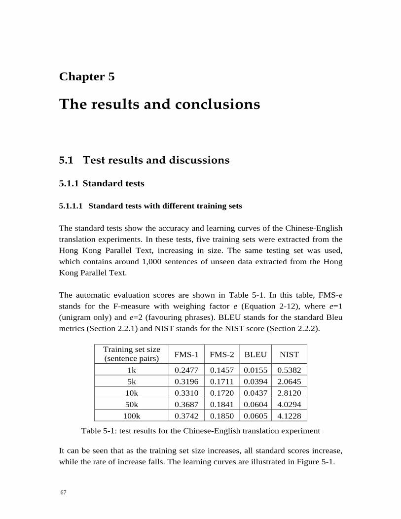
67
Chapter 5
The results and conclusions
5.1 Test results and discussions 5.1.1 Standard tests 5.1.1.1 Standard tests with different training sets The standard tests show the accuracy and learning curves of the Chinese-English translation experiments. In these tests, five training sets were extracted from the Hong Kong Parallel Text, increasing in size. The same testing set was used, which contains around 1,000 sentences of unseen data extracted from the Hong Kong Parallel Text. The automatic evaluation scores are shown in 451HTable 5-1. In this table, FMS-e stands for the F-measure with weighing factor e (Equation 452H2-12), where e=1 (unigram only) and e=2 (favouring phrases). BLEU stands for the standard Bleu metrics (Section 453H2.2.1) and NIST stands for the NIST score (Section 454H2.2.2).
Training set size (sentence pairs) FMS-1 FMS-2 BLEU NIST
1k 0.2477 0.1457 0.0155 0.5382 5k 0.3196 0.1711 0.0394 2.0645
10k 0.3310 0.1720 0.0437 2.8120 50k 0.3687 0.1841 0.0604 4.0294
100k 0.3742 0.1850 0.0605 4.1228
Table 5-1: test results for the Chinese-English translation experiment It can be seen that as the training set size increases, all standard scores increase, while the rate of increase falls. The learning curves are illustrated in 455HFigure 5-1.

68
Standard test: FMS-1
0
0.05
0.1
0.15
0.2
0.25
0.3
0.35
0.4
0 50 100
Size of training set
FMS-1
Standard test: FMS-2
0
0.02
0.04
0.06
0.08
0.1
0.12
0.14
0.16
0.18
0.2
0 50 100
Size of training set
FMS-2
(a) FMS-1 (b) FMS-2
Standard test: BLEU
0
0.01
0.02
0.03
0.04
0.05
0.06
0.07
0 50 100
Size of training set
BLEU
Standard test: NIST
0
0.5
1
1.5
2
2.5
3
3.5
4
4.5
0 50 100
Size of training set
NIST
(c) BLEU (b) NIST
Figure 5-1: the learning curves 5.1.1.2 Example sentences from translation output The following table contains randomly extracted example translations. For each source sentence, the output translations with different training sets are contrasted.
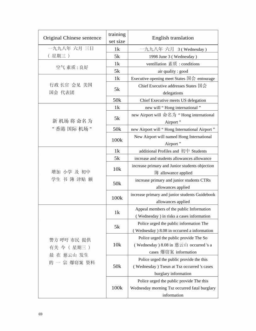
69
Original Chinese sentence training set size
English translation
1k 一九九八年 六月 3 ( Wednesday ) 一九九八年 六月 三日
( 星期三 )
5k 1998 June 3 ( Wednesday )
1k ventillation 素质 : conditions : 空气 素质 良好
5k air quality : good
1k Executive opening meet States 国会 entourage
5k Chief Executive addresses States 国会
delegations
行政 长官 会见 美国
国会 代表团
50k Chief Executive meets US delegation
1k new will “ Hong international ”
5k new Airport will 命名为 “ Hong international
Airport ”
50k new Airport will “ Hong International Airport ”
" "新 机场 将 命名为
香港 国际 机场
100k New Airport will named Hong International
Airport ”
1k additional Profiles and 初中 Students
5k increase and students allowances allowance
10k increase primary and Junior students objection
簿 allowance applied
50k increase primary and junior students CTRs
allowances applied
增加 小学 及 初中
学生 书 簿 津贴 额
100k increase primary and junior students Guidebook
allowances applied
1k Appeal members of the public Information ( Wednesday ) in risks a cases information
5k Police urged the public information The
( Wednesday ) 8.08 in occurred a information
10k Police urged the public provide The So
( Wednesday ) 8.08 in 慈云山 occurred 's a cases 爆窃案 information
50k Police urged the public provide the this
( Wednesday ) Tseun at Tsz occurred 's cases burglary information
警方 呼吁 市民 提供
有关 今 ( 星期三 )
晨 在 慈云山 发生
的 一 宗 爆窃案 资料
100k Police urged the public provide The this
Wednesday morning Tsz occurred fatal burglary information
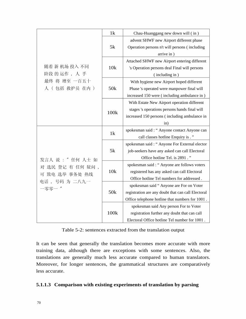
70
1k Chau-Huanggang new down will ( in )
5k advent SHWF new Airport different phase
Operation persons n't will persons ( including arrive in )
10k Attached SHWF new Airport entering different
's Operation persons deal Final will persons ( including in )
50k With hygiene new Airport hoped different Phase 's operated were manpower final will
increased 150 were ( including ambulance in )
随着 新 机场 投入 不同
阶段 的 运作 , 人 手
最终 将 增至 一百五十
人 ( 包括 救护员 在内 )
100k
With Estate New Airport operation different stages 's operations persons hands final will
increased 150 persons ( including ambulance in in)
1k spokesman said : “ Anyone contact Anyone can
call classes hotline Enquiry is . ”
5k spokesman said : “ Anyone For External elector
job-seekers have any asked can call Electoral Office hotline Tel. is 2891 . ”
10k spokesman said : “ Anyone are follows voters
registered has any asked can call Electoral Office hotline Tel numbers for addressed .
50k spokesman said “ Anyone are For on Voter
registration are any doubt that can call Electoral Office telephone hotline that numbers for 1001 .
发言人 说 : " 任何 人士 如
对 选民 登记 有 任何 疑问 ,
可 致电 选举 事务处 热线
电话 , 号码 为 二八九一
一零零一 "
100k spokesman said Any person For to Voter registration further any doubt that can call
Electoral Office hotline Tel number for 1001 .
Table 5-2: sentences extracted from the translation output It can be seen that generally the translation becomes more accurate with more training data, although there are exceptions with some sentences. Also, the translations are generally much less accurate compared to human translators. Moreover, for longer sentences, the grammatical structures are comparatively less accurate. 5.1.1.3 Comparison with existing experiments of translation by parsing
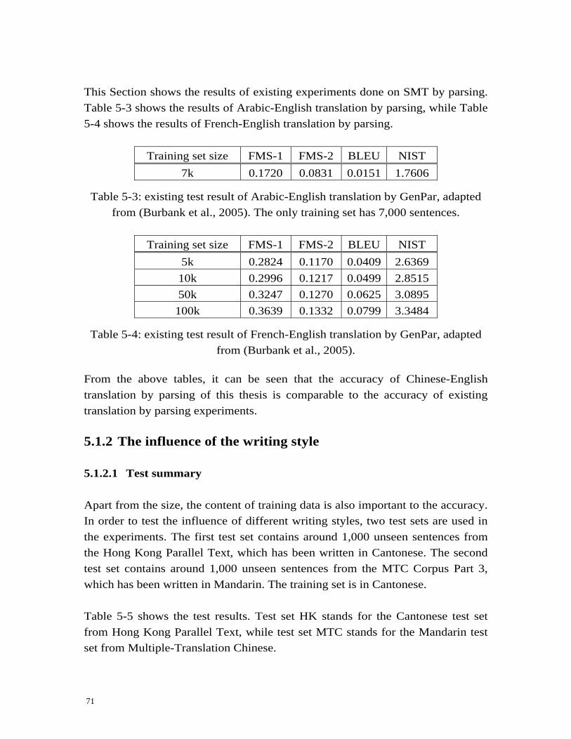
71
This Section shows the results of existing experiments done on SMT by parsing. Table 5-3 shows the results of Arabic-English translation by parsing, while Table 5-4 shows the results of French-English translation by parsing.
Training set size FMS-1 FMS-2 BLEU NIST 7k 0.1720 0.0831 0.0151 1.7606
Table 5-3: existing test result of Arabic-English translation by GenPar, adapted from (Burbank et al., 2005). The only training set has 7,000 sentences.
Training set size FMS-1 FMS-2 BLEU NIST
5k 0.2824 0.1170 0.0409 2.6369 10k 0.2996 0.1217 0.0499 2.8515 50k 0.3247 0.1270 0.0625 3.0895
100k 0.3639 0.1332 0.0799 3.3484
Table 5-4: existing test result of French-English translation by GenPar, adapted from (Burbank et al., 2005).
From the above tables, it can be seen that the accuracy of Chinese-English translation by parsing of this thesis is comparable to the accuracy of existing translation by parsing experiments. 5.1.2 The influence of the writing style 5.1.2.1 Test summary Apart from the size, the content of training data is also important to the accuracy. In order to test the influence of different writing styles, two test sets are used in the experiments. The first test set contains around 1,000 unseen sentences from the Hong Kong Parallel Text, which has been written in Cantonese. The second test set contains around 1,000 unseen sentences from the MTC Corpus Part 3, which has been written in Mandarin. The training set is in Cantonese. Table 5-5 shows the test results. Test set HK stands for the Cantonese test set from Hong Kong Parallel Text, while test set MTC stands for the Mandarin test set from Multiple-Translation Chinese.
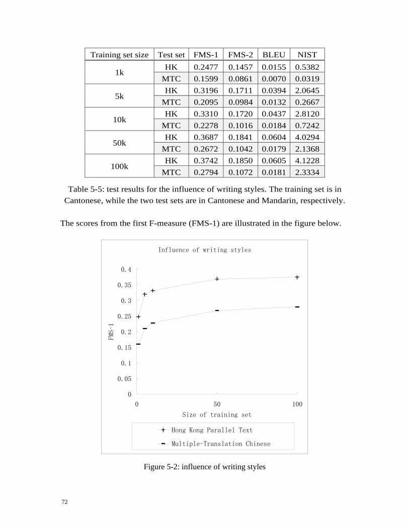
72
Training set size Test set FMS-1 FMS-2 BLEU NIST HK 0.2477 0.1457 0.0155 0.5382
1k MTC 0.1599 0.0861 0.0070 0.0319 HK 0.3196 0.1711 0.0394 2.0645
5k MTC 0.2095 0.0984 0.0132 0.2667 HK 0.3310 0.1720 0.0437 2.8120
10k MTC 0.2278 0.1016 0.0184 0.7242 HK 0.3687 0.1841 0.0604 4.0294
50k MTC 0.2672 0.1042 0.0179 2.1368 HK 0.3742 0.1850 0.0605 4.1228
100k MTC 0.2794 0.1072 0.0181 2.3334
Table 5-5: test results for the influence of writing styles. The training set is in Cantonese, while the two test sets are in Cantonese and Mandarin, respectively.
The scores from the first F-measure (FMS-1) are illustrated in the figure below.
Influence of writing styles
0
0.05
0.1
0.15
0.2
0.25
0.3
0.35
0.4
0 50 100
Size of training set
FMS-1
Hong Kong Parallel Text
Multiple-Translation Chinese
Figure 5-2: influence of writing styles
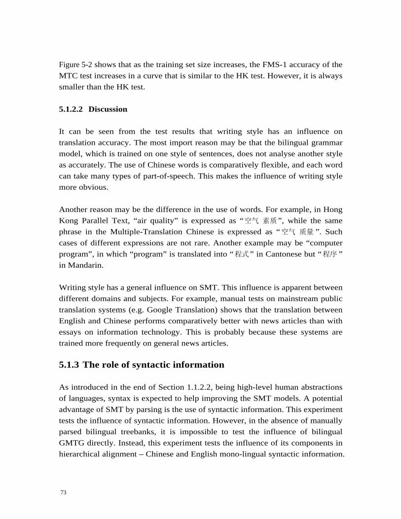
73
459HFigure 5-2 shows that as the training set size increases, the FMS-1 accuracy of the MTC test increases in a curve that is similar to the HK test. However, it is always smaller than the HK test. 5.1.2.2 Discussion It can be seen from the test results that writing style has an influence on translation accuracy. The most import reason may be that the bilingual grammar model, which is trained on one style of sentences, does not analyse another style as accurately. The use of Chinese words is comparatively flexible, and each word can take many types of part-of-speech. This makes the influence of writing style more obvious. Another reason may be the difference in the use of words. For example, in Hong Kong Parallel Text, “air quality” is expressed as “空气 素质”, while the same phrase in the Multiple-Translation Chinese is expressed as “空气 质量 ”. Such cases of different expressions are not rare. Another example may be “computer program”, in which “program” is translated into “程式” in Cantonese but “程序 ” in Mandarin. Writing style has a general influence on SMT. This influence is apparent between different domains and subjects. For example, manual tests on mainstream public translation systems (e.g. Google Translation) shows that the translation between English and Chinese performs comparatively better with news articles than with essays on information technology. This is probably because these systems are trained more frequently on general news articles. 5.1.3 The role of syntactic information As introduced in the end of Section 460H1.1.2.2, being high-level human abstractions of languages, syntax is expected to help improving the SMT models. A potential advantage of SMT by parsing is the use of syntactic information. This experiment tests the influence of syntactic information. However, in the absence of manually parsed bilingual treebanks, it is impossible to test the influence of bilingual GMTG directly. Instead, this experiment tests the influence of its components in hierarchical alignment – Chinese and English mono-lingual syntactic information.
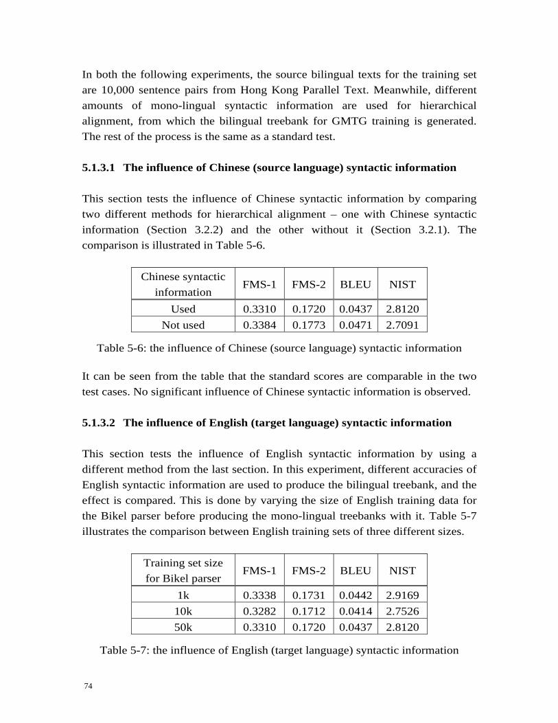
74
In both the following experiments, the source bilingual texts for the training set are 10,000 sentence pairs from Hong Kong Parallel Text. Meanwhile, different amounts of mono-lingual syntactic information are used for hierarchical alignment, from which the bilingual treebank for GMTG training is generated. The rest of the process is the same as a standard test. 5.1.3.1 The influence of Chinese (source language) syntactic information This section tests the influence of Chinese syntactic information by comparing two different methods for hierarchical alignment – one with Chinese syntactic information (Section 3.2.2) and the other without it (Section 3.2.1). The comparison is illustrated in Table 5-6.
Chinese syntactic information
FMS-1 FMS-2 BLEU NIST
Used 0.3310 0.1720 0.0437 2.8120 Not used 0.3384 0.1773 0.0471 2.7091
Table 5-6: the influence of Chinese (source language) syntactic information It can be seen from the table that the standard scores are comparable in the two test cases. No significant influence of Chinese syntactic information is observed. 5.1.3.2 The influence of English (target language) syntactic information This section tests the influence of English syntactic information by using a different method from the last section. In this experiment, different accuracies of English syntactic information are used to produce the bilingual treebank, and the effect is compared. This is done by varying the size of English training data for the Bikel parser before producing the mono-lingual treebanks with it. Table 5-7 illustrates the comparison between English training sets of three different sizes.
Training set size for Bikel parser
FMS-1 FMS-2 BLEU NIST
1k 0.3338 0.1731 0.0442 2.9169 10k 0.3282 0.1712 0.0414 2.7526 50k 0.3310 0.1720 0.0437 2.8120
Table 5-7: the influence of English (target language) syntactic information

75
It can be seen from the table that the standard scores are comparable in the three test cases. No significant influence of English syntactic information is observed. 5.1.3.3 Conclusion In the above experiments, neither English nor Chinese mono-lingual syntactic information has a significant influence on the standard evaluation scores. There are two possible reasons for this. Firstly, the accuracy of GMTG may have no significant impact on translation. That is to say, syntactic information does not play an important role in Chinese-English SMT by GMTG parsing. In comparison, Och et al. (2004) examined the influence of various features on a maximum entropy SMT model, and found no significant influence of syntactic information. However, recent research by Quirk and Corston-Oliver (2006) shows the influence of English syntactic information on a different tree-based SMT model, which combines phrase-based information with syntactic treelets. Therefore, it may be concluded that the role of syntactic information on SMT is dependent on the probabilistic model, and with probabilistic GMTG, syntax information is comparatively less influential. However, the above conclusion can only be confirmed with the availability of confidently accurate (i.e. manually parsed) bilingual treebanks. The second possible reason for the experiment result is the noise in hierarchical alignment, which is currently a necessary step to derive bilingual treebanks. This noise may come from the inaccuracy of mono-lingual parsers, the word alignment algorithm, as well as the hierarchical alignment process. What is more, sentence pairs from the Hong Kong Parallel Text are correspondent in meaning, instead of CFG structures. By observation, there are over 20% sentence pairs that are not syntactically correspondent to each other. The noise in the resulting bilingual treebank can be significant enough to outweigh the influence of mono-lingual syntactic information. 5.1.4 The importance of word-to-word probabilities 5.1.4.1 Test summary Most current SMT systems are based on word-to-word translations. In the
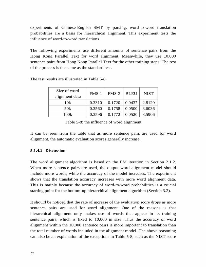
76
experiments of Chinese-English SMT by parsing, word-to-word translation probabilities are a basis for hierarchical alignment. This experiment tests the influence of word-to-word translations. The following experiments use different amounts of sentence pairs from the Hong Kong Parallel Text for word alignment. Meanwhile, they use 10,000 sentence pairs from Hong Kong Parallel Text for the other training steps. The rest of the process is the same as the standard test. The test results are illustrated in Table 5-8.
Size of word alignment data
FMS-1 FMS-2 BLEU NIST
10k 0.3310 0.1720 0.0437 2.8120 50k 0.3560 0.1758 0.0500 3.6036
100k 0.3596 0.1772 0.0520 3.5906
Table 5-8: the influence of word alignment It can be seen from the table that as more sentence pairs are used for word alignment, the automatic evaluation scores generally increase. 5.1.4.2 Discussion The word alignment algorithm is based on the EM iteration in Section 2.1.2. When more sentence pairs are used, the output word alignment model should include more words, while the accuracy of the model increases. The experiment shows that the translation accuracy increases with more word alignment data. This is mainly because the accuracy of word-to-word probabilities is a crucial starting point for the bottom-up hierarchical alignment algorithm (Section 3.2). It should be noticed that the rate of increase of the evaluation score drops as more sentence pairs are used for word alignment. One of the reasons is that hierarchical alignment only makes use of words that appear in its training sentence pairs, which is fixed to 10,000 in size. Thus the accuracy of word alignment within the 10,000 sentence pairs is more important to translation than the total number of words included in the alignment model. The above reasoning can also be an explanation of the exceptions in Table 5-8, such as the NIST score
77
with 100k sentence pairs. Word-to-word translation is generally crucial to SMT. From the human translation’s point of view, words and unbreakable phrases are also the basic elements to be translated. Finally, it should be noted that SMT by GMTG parsing is based on words instead of phrases – phrases are not considered separately as terminal symbols in GMTG, but integrated into the production rules. This is a potential disadvantage to the model. As a result, SMT by GMTG parsing may also have the problem of word-based models discussed in Section 469H2.1.3. What is more, the word based alignment may result in lower Bleu scores than phrase-based models, since the Bleu evaluation is based on n-grams. This is less important, however, as long as the translation is reasonable by the human evaluation.
5.2 Summary Like human translation, machine translation has two essential factors – unit element (unbreakable word or phrase that carries meaning) translation and target sentence organisation. The simplest models for SMT are word-based, where the unit elements are words and sentence organisation is modelled by comparatively simple mechanisms such as word reordering. One of the main improvements of phrase-based models over the word-based models is on the definition of unit elements, which includes phrases. Hierarchical phrase based and tree-based models further improved the target sentence organisation. The models have improved translation accuracy by evolving towards a higher level of abstraction, while word alignment often serves as the basis for more complex models. SMT by parsing can be seen as using a tree-based model. It also makes use of syntactic information, which has been helpful to SMT systems in modelling hierarchical constituent movement and target language generation. The decoding process for SMT by parsing is special in that the translation sentence is generated as a by-product of parsing with bilingual synchronous grammars, which requires recursive correspondence between the grammatical structures of the two languages. The advantages of this decoding process include the reuse of existing parsing algorithms to save engineering cost.
78
Chinese-English SMT is a special instance of statistical machine translation. While it benefits from general SMT methods, it is also influenced by the specific properties of both languages. Based on the GenPar system and other pieces of software, this thesis studies Chinese-English SMT by bilingual GMTG parsing with large-scale experiments. The results show that the accuracy of Chinese-English translation by parsing is comparable with existing French-English and Arabic-English translations by GMTG parsing from the literature. What is more, although word-alignment has significant influence on translation, mono-lingual syntactic Chinese and English information is not as influential in the experiments. The experiments also reveal that SMT systems have much to improve. For example, the overall accuracy is still far below human translation, and the effect of translation is considerably influenced by writing style and topic. From the above experiments, several possible further improvements can be suggested. They are discussed in the next section.
5.3 Future work This section presents possible improvements to SMT models. The possible future works are organised by the two main factors summarised in the last section – unit element translation and sentence organisation. The word-to-word and phrase-to-phrase alignment models are crucial to any SMT system. Because words and phrases are the atomic elements that carry the meaning of a sentence, it is likely that a translation is understandable with words and phrases correctly translated, even if the order is inaccurate. Currently most SMT systems use EM based learning methods, while there are Chinese-English dictionaries available without probabilities. A possible improvement is making use of off-the-shelf dictionaries during the training of word and phrase alignments. Another observation from the experiments is that word translations can be dependent on context. A word can have many different translations, while for a certain source sentence there is a best choice. Thus it is reasonable to consider a word-to-word model that includes contextual information explicitly. The difficulty is the choice of context. When grammar is considered, an example
79
context may be the head word. Sentence organisation can be improved by better models, while syntactic information is an important factor. In the experiments of Chinese-English SMT by synchronous GMTG parsing, mono-lingual syntactic information did not prove to have a significant influence. Apart from the noise introduced by the hierarchical alignment, some further thoughts arise about the model itself: Firstly, there is the possibility that the accuracy of bilingual GMTG (or combined CFG) does not have a significant influence. The above possibility can only be demonstrated when the corresponding Chinese-English bilingual treebank is available in a reasonable size in the future. Meanwhile, it is meaningful to think of potentially better representation of the correspondence between Chinese and English sentences. As was seen from the Hong Kong Parallel Text, a significant amount of parallel sentences are correspondent in meaning, but not in CFG syntactic structures. Therefore, the candidates which express more common structural alignment between translation pairs may include more semantic-prone grammar structures, such as the lexical functional grammar (LFG; Dalrymple, 2001) and combinatory categorical grammar (CCG; Steedman, 2000). Secondly, potentially better models may also use no hierarchical structural combination. On the one hand, the same meaning can be best carried out by completely different syntactic structures in Chinese and English. On the other hand, mono-lingual syntactic information is clearly helpful in the generation of sentences. Therefore, it may be useful to consider a two-phase decoding model that does not include any recursive structural correspondence, but separates source sentence analysis and target sentence generation. In this way the target language grammar can be used specifically for generating translations. What is more, grammatical information for only one language, such as the tense of English sentences, can be explicitly modelled. The difficulty is the intermediate representation, and the disadvantage of this model is that existing techniques in generalised parsing may be inapplicable for reuse.
80
References
A. Aho and J. Ullman. 1969. Syntax directed translations and the pushdown assembler. Journal of Computer and System Sciences, 3: 37–56, February.
James Allen. 1995. Natural Language Understanding (2nd edition). Addison-Wesley.
Yaser Al-Onaizan, Jan Curin, Michael Jahr, Kevin Knight, John Lafferty, Dan Melamed, Franz-Josef Och, David Purdy, Noah A. Smith, David Yarowsky. 1999. Statistical Machine Translation Final Report. JHU Workshop 1999.
James Baker. 1979. Trainable grammars for speech recognition. In Speech Communications Papers for the 97th Meeting of the Acoustical Society of America, pp. 547–550, Boston, MA, June.
Daniel Bikel. 2002. Design of a Multi-lingual, Parallel-processing Statistical Parsing Engine. In Human Language Technology Conference (HLT), San Diego.
A. Burbank, M. Carpuat, S. Clark, M. Dreyer, P. Fox, D. Groves, K. Hall, M. Hearne, D. Melamed, Y. Shen, A. Way, B. Wellington, and D. Wu. 2005. Final Report of the 2005 Language Engineering Workshop on Statistical Machine Translation by Parsing. JHU Workshop 2005.
Brooke Cowan, Ivona Kucerova, and Michael Collins. 2006. A Discriminative Model for Tree-to-Tree Translation. To appear in proceedings of the Conference on Empirical Methods in Natural Language Processing 2006.
Peter F. Brown, Vincent J. Della Pietra, Peter V. deSouza, Jenifer C. Lai, Robert L. Mercer. 1990. Class-Based N-Gram Models of Natural Language. Computational Linguistics, 16(2): 79–85.
Peter F. Brown, Stephen A. Della Pietra, Vincent J.Della Pietra, Robert. L. Mercer. 1993. The mathematics of statistical machine translation: Parameter estimation. Computational Linguistics, 19(2): 263–311.
Eugene Charniak. 2000. A maximum-entropy-inspired parser. In Proceedings of North American ACL (NAACL), pp, 132–139.
David Chiang. 2005. A Hierarchical Phrase-Based Model for Statistical Machine Translation. In Proceedings of ACL-05, pp. 263–270.
Noam Chomsky. 1956. Three models for the description of language. I.R.E. Transactions on Information Theory, vol. IT-2, no. 3: 113–24.
113HJohn Cocke and Jacob T. Schwartz. 1970. Programming languages and their compilers: Preliminary notes. Technical report, Courant Institute of
81
Mathematical Sciences, New York University, 1970.22.
Michael Collins. 1996. A New Statistical Parser Based on Bigram Lexical Dependencies. In Proceedings of ACL-96, pp. 184–191.
Michael Collins. 1997. Three Generative, Lexicalised Models for Statistical Parsing. In Proceedings of the ACL-97, pp. 16–23, Madrid, Spain, July.
Thomas H. Cormen, Charles E. Leiserson, Ronald L. Rivest, and Clifford Stein. 2001. Introduction to Algorithms, Secion Edition. MIT Press & McGraw-Hill.
Mary Dalrymple. 2001. Lexical Functional Grammar. New York: Academic Press.
George Doddington. 2002. Automatic evaluation of machine translation quality using n-gram cooccurrence statistics. ARPA Workshop on Human Language Technology.
Jay Earley. 1970. An efficient context-free parsing algorithm. Communications of the Association for Computing Machinery, 13(2): 94–102.
Roger Garside, Geoffrey Leech and Geoffrey Sampson. 1987. The Computation-al Analysis of English: A Corpus-based Approach. London: Longman.
Daniel Gildea. 2003. Loosely Tree-Based Alignment for Machine Translation. In Proceedings of ACL-03, pp. 80–87, Sapporo, Japan.
Joshua Goodman. 1998. Parsing Inside-out. Ph.D. Thesis, Harvard University.
John Hutchins. 2005. The history of machine translation in a nutshell. http://ourworld.compuserve.com/homepages/wjhutchins/Nutshell.htm
Frederick Jelinek. 1969. A fast sequential decoding algorithm using a stack. IBM Journal of Research and Development, vol. 13, pp. 675–685, 1969.
Daniel Jurafsky and James H. Martin. 2000. An Introduction to Natural Language Processing, Computational Linguistics, and Speech Recognition. Prentice-Hall.
T. Kasami. 1965. An efficient recognition and syntax-analysis algorithm for context-free languages. Technical report AFCRL-65758, Air Force Cambridge Research Laboratory.
Kevin Knight, Daniel Marcu. 2004. Machine Translation in the Year 2004. In Intl. Conf. on Acoustics, Speech, and Signal Processing (ICASSP), 965–968.
Philipp Koehn, Franz Josef Och, Daniel Marcu. 2003. Statistical Phrase-Based Translation. In Proceedings of HLT, pp. 127–133.
Karim Lari, Steve J. Young. 1990. The estimation of stochastic context-free grammars using the inside-outside algorithm. Computer Speech and Language, 4: 35–56, 1990.
Robert Lowth. 1762. A Short Introduction to English Grammar. Scholars Facsimilies & Reprint.
David Magerman. 1995. Parsing as Statistical Pattern Recognition. Ph.D. Thesis,
82
Stanford University.
David McClosky, Eugene Charniak, Mark Johnson. 2006. Effective Self-Training for Parsing. In Proceedings of North American ACL (NAACL).
I. Dan Melamed. 2003. Multitext Grammars and Synchronous Parsers. In Proceedings of the 2003 Meeting of the North American chapter of the Association for Computational Linguistics (NAACL-03), Edmonton.
I. Dan Melamed, Giorgio Satta and Benjamin Wellington. 2004. Generalized multitext grammars. In Proceedings of ACL-04, Barcelona, Spain.
I. Dan Melamed, Wei Wang. 2005. Statistical Machine Translation by Generalized Parsing. Proteus Project Working Paper #2.
Daniel Marcu and William Wong. 2002. A phrase-based, joint probability model for statistical machine translation. In Proceedings of the Conference on Empirical Methods in Natural Language Processing.
Franz Josef Och. 1999. An Efficient Method for Determining Bilingual Word Classes. In Proceedings of EACL-99, Bergen, Norway.
Franz Josef Och, Christoph Tillman and Hermann Ney. 1999. Improved alignment models for statistical machine translation. In Proceedings of the Joint Conference on Empirical Methods in Natural Language Processing and Very Large Corpora (in conjunction with ACL-99), pp. 20–28, College Park, MD, USA, June.
Franz Josef Och, Hermann Ney. 2000. Improved Statistical Alignment Models. In Proceedings of ACL-2000, pp. 440–447, Hong Kong, China, October.
Franz Josef Och and Hermann Ney. 2002. Discriminative Training and Maximum Entropy Models for Statistical Machine Translation. In Proceedings of Annual Meeting of the Association for Computational Linguistics, pp. 295–302, Philadelphia, PA, July.
Franz Josef Och, Hermann Ney. 2003. A Systematic Comparison of Various Statistical Alignment Models. Computational Linguistics, 29(1): 19–51.
Franz Josef Och, Daniel Gildea, Sanjeev Khudanpur, Anoop Sarkar, Kenji Yamada, Alex Fraser, Shankar Kumar, Libin Shen, David Smith, Katherine Eng, Viren Jain, Zhen Jin and Dragomir Radev. 2004. A Smorgasbord of Features for Statistical Machine Translation. In Proceedings of HLT/NAACL 2004, Boston.
Kishore Papineni, Salim Roukos, Todd Ward, Wei-Jing Zhu. 2001. BLEU: A Method for Automatic Evaluation of Machine Translation. In Proceedings of ACL-02, pp. 311–318, Philadelphia, PA, July.
Chris Quirk and Simon Corston-Oliver. 2006. The impact of parse quality on syntactically-informed statistical machine translation. To appear in proceedings of the Conference on Empirical Methods in Natural Language Processing 2006.
Adwait Ratnaparkhi. 1997. A simple introduction to maximum entropy models for natural language processing. IRCS Report 97-08, University of Pennsylvania, 3401 Walnut Street, Suite 400A, Philadelphia, PA, May.
83
Azriel Rosenfeld. 1968. An Introduction to Algebraic Structures. New York, Holden-Day.
Stuart Russell and Peter Norvig. 2003. Artificial Intelligence: A Modern Approach (Second Edition). Prentice Hall.
Geoffrey Sampson. 1986. Simulated Annealing as a Parsing Technique. In University of Leeds Working Papers in Linguistics and Phonetics 4: 43–60.
Mark Steedman. 2000. The Syntactic Process. MIT Press.
Chrostoph Tillmann, Stephan Vogel, Hermann Ney and Alex Zubiaga. 1997. A DPbased Search Using Monotone Alignments in Statistical Translation. In Proceedings of ACL/EACL-97, pp. 289–296, Madrid, Spain, July.
Kristina Toutanova and Christopher D. Manning. 2000. Enriching the Knowledge Sources Used in a Maximum Entropy Part-of-Speech Tagger. In Proceedings of the Conference on Empirical Methods in Natural Language Processing.
Joseph Turian, Luke Shen, I. Dan Melamed. 2003. Evaluation of Machine Translation and its Evaluation. In Proceedings of MT Summit IX, pp. 386–393, New Orleans, LA, September.
Stephan Vogel, Hermann Ney, Christoph Tillmann. 1996. HMM-based word alignment in statistical translation. In Proceedings of ACL-96, pp. 836–841, Copenhagen, Denmark, August.
Dekai Wu. 1997. Stochastic Inversion Transduction Grammars and Bilingual Parsing of Parallel Corpora. Computational Linguistics, 23(3): 377–404.
Kenji Yamada and Kevin Knight. 2001. A syntax-based statistical translation model. In Proceedings of ACL-01, pp. 523–529, Toulouse, France.
Daniel H. Younger. 1967. Recognition and parsing of context-free languages in time n3. Information and Control, 10(2): 189–208.
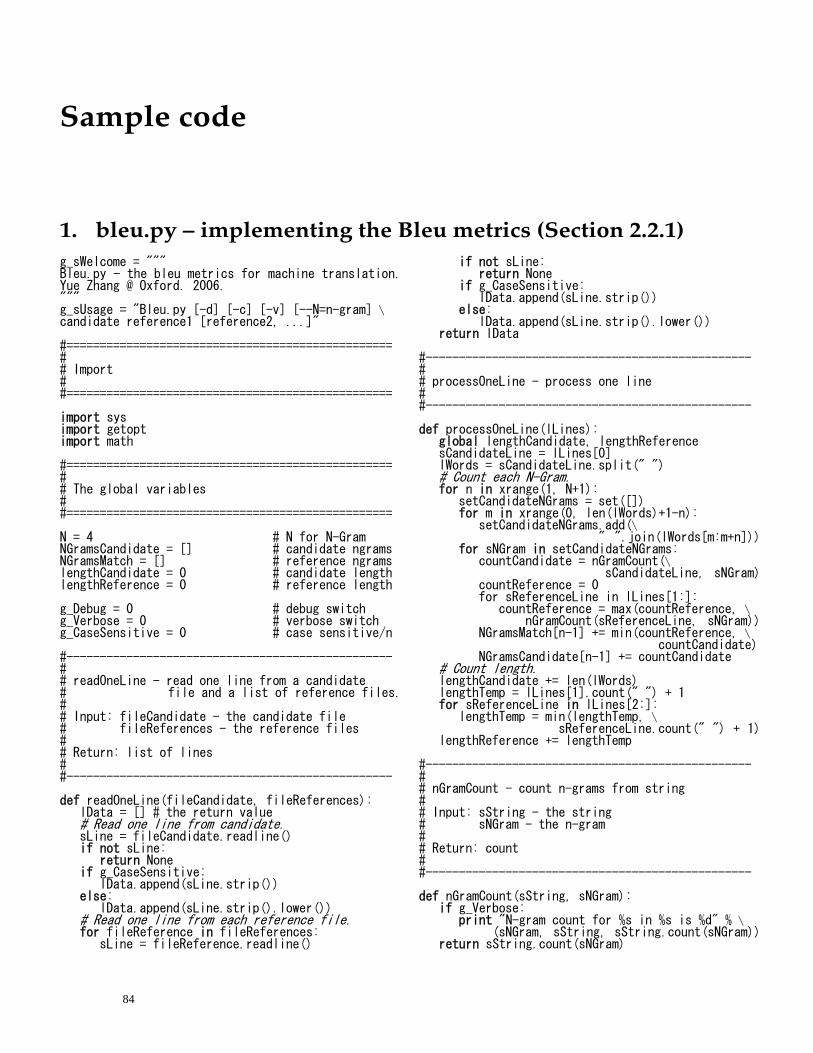
84
Sample code
1. bleu.py – implementing the Bleu metrics (Section 470H2.2.1)
g_sWelcome = """ Bleu.py - the bleu metrics for machine translation. Yue Zhang @ Oxford. 2006. """ g_sUsage = "Bleu.py [-d] [-c] [-v] [--N=n-gram] \ candidate reference1 [reference2, ...]" #================================================= # # Import # #================================================= import sys import getopt import math #================================================= # # The global variables # #================================================= N = 4 # N for N-Gram NGramsCandidate = [] # candidate ngrams NGramsMatch = [] # reference ngrams lengthCandidate = 0 # candidate length lengthReference = 0 # reference length g_Debug = 0 # debug switch g_Verbose = 0 # verbose switch g_CaseSensitive = 0 # case sensitive/n #------------------------------------------------- # # readOneLine - read one line from a candidate # file and a list of reference files. # # Input: fileCandidate - the candidate file # fileReferences - the reference files # # Return: list of lines # #------------------------------------------------- def readOneLine(fileCandidate, fileReferences): lData = [] # the return value # Read one line from candidate. sLine = fileCandidate.readline() if not sLine: return None if g_CaseSensitive: lData.append(sLine.strip()) else: lData.append(sLine.strip().lower()) # Read one line from each reference file. for fileReference in fileReferences: sLine = fileReference.readline()
if not sLine: return None if g_CaseSensitive: lData.append(sLine.strip()) else: lData.append(sLine.strip().lower()) return lData #------------------------------------------------- # # processOneLine - process one line # #------------------------------------------------- def processOneLine(lLines): global lengthCandidate, lengthReference sCandidateLine = lLines[0] lWords = sCandidateLine.split(" ") # Count each N-Gram. for n in xrange(1, N+1): setCandidateNGrams = set([]) for m in xrange(0, len(lWords)+1-n): setCandidateNGrams.add(\
" ".join(lWords[m:m+n])) for sNGram in setCandidateNGrams: countCandidate = nGramCount(\
sCandidateLine, sNGram) countReference = 0 for sReferenceLine in lLines[1:]: countReference = max(countReference, \
nGramCount(sReferenceLine, sNGram)) NGramsMatch[n-1] += min(countReference, \
countCandidate) NGramsCandidate[n-1] += countCandidate # Count length. lengthCandidate += len(lWords) lengthTemp = lLines[1].count(" ") + 1 for sReferenceLine in lLines[2:]: lengthTemp = min(lengthTemp, \
sReferenceLine.count(" ") + 1) lengthReference += lengthTemp #------------------------------------------------- # # nGramCount - count n-grams from string # # Input: sString - the string # sNGram - the n-gram # # Return: count # #------------------------------------------------- def nGramCount(sString, sNGram): if g_Verbose: print "N-gram count for %s in %s is %d" % \
(sNGram, sString, sString.count(sNGram)) return sString.count(sNGram)
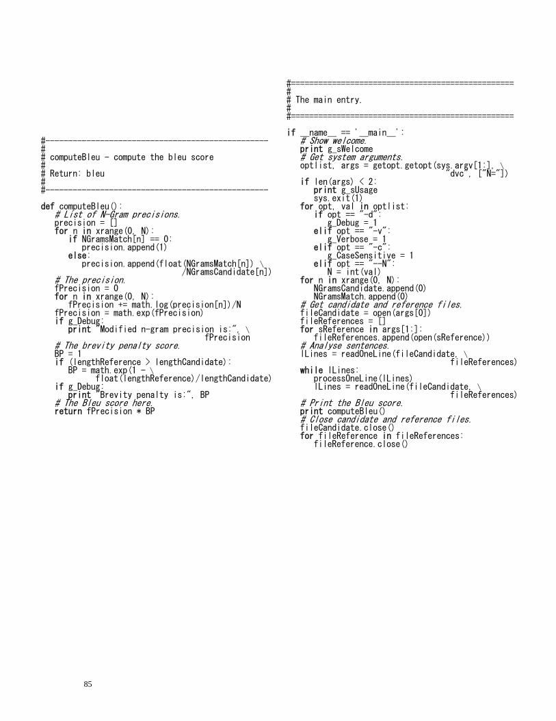
85
#------------------------------------------------- # # computeBleu - compute the bleu score # # Return: bleu # #------------------------------------------------- def computeBleu(): # List of N-Gram precisions. precision = []
for n in xrange(0, N): if NGramsMatch[n] == 0: precision.append(1) else: precision.append(float(NGramsMatch[n]) \
/NGramsCandidate[n]) # The precision. fPrecision = 0 for n in xrange(0, N): fPrecision += math.log(precision[n])/N fPrecision = math.exp(fPrecision) if g_Debug: print "Modified n-gram precision is:", \
fPrecision # The brevity penalty score. BP = 1 if (lengthReference > lengthCandidate): BP = math.exp(1 - \
float(lengthReference)/lengthCandidate) if g_Debug: print "Brevity penalty is:", BP # The Bleu score here. return fPrecision * BP
#================================================= # # The main entry. # #================================================= if __name__ == '__main__': # Show welcome. print g_sWelcome # Get system arguments. optlist, args = getopt.getopt(sys.argv[1:], \
"dvc", ["N="]) if len(args) < 2: print g_sUsage sys.exit(1) for opt, val in optlist: if opt == "-d": g_Debug = 1 elif opt == "-v": g_Verbose = 1 elif opt == "-c": g_CaseSensitive = 1 elif opt == "--N": N = int(val) for n in xrange(0, N): NGramsCandidate.append(0) NGramsMatch.append(0) # Get candidate and reference files. fileCandidate = open(args[0]) fileReferences = [] for sReference in args[1:]: fileReferences.append(open(sReference)) # Analyse sentences. lLines = readOneLine(fileCandidate, \
fileReferences) while lLines: processOneLine(lLines) lLines = readOneLine(fileCandidate, \
fileReferences) # Print the Bleu score. print computeBleu() # Close candidate and reference files. fileCandidate.close() for fileReference in fileReferences: fileReference.close()
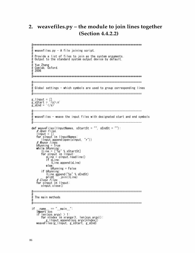
86
2. weavefiles.py – the module to join lines together (Section 471H4.4.2.2)
#******************************************************************** # # weavefiles.py - A file joining script. # # Provide a list of files to join as the system arguments. # Output to the standard system output device by default. # # Yue Zhang # Comlab, Oxford. # 2006 # #******************************************************************** #==================================================================== # # Global settings - which symbols are used to group corresponding lines # #==================================================================== g_lInput = [] g_sStart = '<s>\n' g_sEnd = '</s>' #-------------------------------------------------------------------- # # weaveFiles - weave the input files with designated start and end symbols # #-------------------------------------------------------------------- def weaveFiles(lInputNames, sStartSt = "", sEndSt = ""): # Open files. lInput = [] for sInput in lInputNames: lInput.append(open(sInput, "r")) # Weave lines. bRunning = True while bRunning: lLine = ["%s" % sStartSt] for oInput in lInput: sLine = oInput.readline() if sLine: lLine.append(sLine) else: bRunning = False if bRunning: lLine.append("%s" % sEndSt) print "".join(lLine) # Close files. for oInput in lInput: oInput.close() #==================================================================== # # The main methods # #==================================================================== if __name__ == "__main__": import sys if len(sys.argv) > 1: for nIndex in xrange(1, len(sys.argv)): g_lInput.append(sys.argv[nIndex]) weaveFiles(g_lInput, g_sStart, g_sEnd)