www.elsevier.com/locate/ygeno

Genomics 83 (2004) 349–360

Minireview

ChIP-chip: considerations for the design, analysis, and application of

genome-wide chromatin immunoprecipitation experiments

Michael J. Buck and Jason D. Lieb*

Department of Biology and Carolina Center for Genome Sciences, CB 3280, 202 Fordham Hall, University of North Carolina at Chapel Hill,

Chapel Hill, NC 27599-3280, USA

Received 3 October 2003; accepted 12 November 2003

Abstract

Chromatin immunoprecipitation (ChIP) is a well-established procedure used to investigate interactions between proteins and DNA.

Coupled with whole-genome DNA microarrays, ChIPs allow one to determine the entire spectrum of in vivo DNA binding sites for any given

protein. The design and analysis of ChIP-microarray (also called ChIP-chip) experiments differ significantly from the conventions used for

more traditional microarray experiments that measure relative transcript levels. Furthermore, fundamental differences exist between single-

locus ChIP approaches and ChIP-chip experiments, and these differences require new methods of analysis. In this light, we review the design

of DNA microarrays, the selection of controls, the level of repetition required, and other critical parameters for success in the design and

analysis of ChIP-chip experiments, especially those conducted in the context of mammalian or other relatively large genomes.

D 2004 Elsevier Inc. All rights reserved.

Introduction

Interactions between proteins and DNA are fundamental

to life. They mediate transcription, DNA replication, recom-

bination, and DNA repair, all processes that are central to

the biology of every organism. A comprehensive under-

standing of where enzymes and their regulatory proteins

interact with the genome in vivo would greatly increase our

understanding of the mechanism and logic of these critical

cellular events. Over the past several years, advances in

technology have made feasible, in selected organisms, the

goal of cataloging all protein–DNA interactions under a

diverse set of physiological conditions.

Traditional methods of investigation have failed to create

high-resolution, genome-wide maps of the interaction be-

tween a DNA-binding protein and DNA. For example, the

DNA-binding properties of a protein determined by in vitro

oligo selection or gel-shift assays are often poor predictors

of a factor’s actual binding targets in vivo [1]. This is

primarily because transcription factors and other eukaryotic

DNA-binding proteins generally recognize degenerate

motifs of 5 to 10 nucleotides. Even in the simple case of

the yeast genome, a typical transcription factor’s binding

0888-7543/$ - see front matter D 2004 Elsevier Inc. All rights reserved.

doi:10.1016/j.ygeno.2003.11.004

* Corresponding author. Fax: +1-919-962-1625.

E-mail address: jlieb@bio.unc.edu (J.D. Lieb).

site may appear several thousand times. The fact that

consensus DNA binding sites occur far too often in genomic

DNA sequence to provide sufficient specificity has also

frustrated the use of computational approaches to identify

binding sites that are active in vivo. When putative sites of

binding can be identified, methods like DNA footprinting or

ChIP followed by quantitative PCR can be used, but are

applicable only to small segments of hand-chosen genomic

loci. Finally, attempts to determine the genome-wide bio-

logical activity of DNA-binding proteins by measuring

relative transcript level changes in cells lacking the protein

of interest often yield secondary consequences of the

deletion, rather than true primary targets of the regulatory

protein [2,3].

The union of chromatin immunoprecipitation (ChIP) and

whole-genome DNA microarrays (ChIP-chip) circumvents

these limitations by allowing researchers to create high-

resolution genome-wide maps of the in vivo interactions

between DNA-associated proteins and DNA. Currently,

there are about the same number of reviews and book

chapters on ChIP-chip procedures and applications [4–13]

as there are primary papers in the literature [1,14–25]. We

will concentrate on the general considerations for the design

and analysis of ChIP-chip experiments, an area that has not

yet been addressed in detail. A concise review of ChIP-chip

procedures and applications is useful for framing that topic.

enomics 83 (2004) 349–360

An overview of the ChIP-chip experimental procedure

Ranging from yeast to cultured mammalian cells, there

is surprisingly little variation in published ChIP-chip pro-

tocols. Generally, cells are grown under the desired exper-

M.J. Buck, J.D. Lieb / G350

Fig. 1. (A) A summary of the ChIP-chip procedure. See the text for details. (B) Com

and microarray-based experiments. Single-locus experiments use a single internal

the IP, mock IP (or control IP), and input DNA. In microarray experiments, rati

obtained for all other elements, which are termed non-enriched. (C) Global array n

median log2 ratio is equal to 0 for the normalized distribution (blue). (D) The eff

20% of arrayed elements detect five-fold enrichment (log2 STDev = 0.5). The s

average ratios are plotted. The distribution is skewed such that the median log2 ratio

would center the non-enriched population at 0 (green).

imental condition and then fixed with formaldehyde (Fig.

1A). Formaldehyde crosslinks proteins to each other pri-

marily between the e-amino group of lysine residues and

an adjacent peptide bond. Formaldehyde can also form

DNA–protein crosslinks, but only if the DNA is partially

parison of the controls used for single-locus, PCR-based ChIP experiments

control in each sample. The intensity of the target band is compared across

os obtained for enriched elements (boxed in white) are compared to those

ormalization will slide the raw distribution (red) along the x-axis so that the

ect of default normalization on a simulated ChIP-chip experiment in which

imulated experiment was repeated three times, and the distribution of the

of the non-enriched population is at �0.25 (black). The ideal normalization

M.J. Buck, J.D. Lieb / Genom

denatured to expose the –CO–NH moiety at position 1

(N-1) of a guanine or the exocyclic amino groups of an

adenine, guanine, or cytosine. The exact nature of the

crosslinks formed by formaldehyde in chromatin in vivo is

not well characterized, and it is unclear whether the

majority of crosslinks formed are protein–protein or pro-

tein–DNA. In some cases, other crosslinking agents like

dimethyl adipimidate have been used in combination with

formaldehyde [6]. However, formaldehyde remains the

most commonly used fixative because the crosslinks are

heat-reversible, which allows downstream enzymatic treat-

ment of the DNA. After crosslinking, the extract is

sonicated to shear the DNA fragments to the desired size,

usually 1 kb or smaller.

DNA fragments crosslinked to the protein of interest are

enriched in one of three standard ways: immunoprecipita-

tion with a protein-specific antibody, immunoprecipitation

of a tagged protein using an antibody specific to the tag, or

affinity purification using a tag that obviates the need for

antibodies, such as the TAP (tandem affinity purification)

tag [26]. The formaldehyde crosslinks are then reversed and

the DNA is purified. Low DNA yields from the IP reactions

usually make DNA amplification a requirement for DNA

microarray-based detection. Randomly-primed [27] or liga-

tion-mediated PCR-based [28] methods have been most

commonly used, but a recently described linear amplifica-

tion method is likely to give higher fidelity results [29].

Ideally, the IPs can be scaled up economically and ampli-

fication can be avoided.

Enriched DNA is then labeled with a fluorescent mole-

cule such as Cy5 or Alexa 647. The fluorescent molecule

can be introduced directly in the form of a modified

nucleotide [30] or by chemical coupling after the introduc-

tion of an aminoallyl nucleotide derivative [31]. In two-

color array platforms, genomic DNA prepared from IP input

extract is generally used as a reference and similarly

amplified and labeled with a different fluor, such as Cy3

or Alexa 555 [21]. The two probes are then combined and

hybridized to a single DNA microarray. Ideally, to provide a

comprehensive and unbiased survey of protein-DNA inter-

actions, the DNA microarrays used in ChIP experiments

contain elements (deposited DNA fragments) that represent

the entire genome.

The results of the hybridization allow one to identify

which segments of the genome were enriched in the IP.

Since the precise location of each arrayed element is known,

construction of a genome-wide map of in vivo protein–

DNA interactions is possible. The resolution of the method

depends mainly on two factors: the length of the sheared

chromatin enriched by the IP and the length and spacing of

the arrayed DNA elements used to detect the IP-enriched

fragments. Typical yeast experiments achieve a resolution of

about 1 kb, which is sufficient to assign binding to the

regulation of a single gene. Once the bound regulatory

region is identified, the exact binding site can often be

inferred by computational methods [32,33].

Successful applications

The ChIP-chip technique was first applied successfully

to identify binding sites for individual transcription factors

in Saccharomyces cerevisiae [1,15,16]. Later, also in yeast,

a c-Myc epitope protein tagging system was used to map

the genome-wide positions of 106 transcription factors

[17]. Other applications have been reported, including

the study of DNA replication [34], recombination [35],

and chromatin structure [23–25,36]. In these experiments,

microarrays containing f1-kb PCR products representing

ORFs (open reading frames), intergenic regions, or both

were used in conjunction with a two-color experimental

scheme. The PCR products in these arrays were ‘‘tiled’’

across the genome, meaning the PCR products were

directly adjacent to one another along the genome, with

little or no DNA sequence between arrayed elements. The

compact and nonrepetitive nature of the simple genomes

harbored by these model organisms made such an ap-

proach feasible.

Experiments in mammalian systems have proven more

difficult due to the large and repetitive nature of their

genomes. Initial ChIP-chip experiments identified binding

sites for the c-Myc, Max, Gata1, E2F, and Rb transcrip-

tion factors in cultured human cells [18,20–22]. For

practical reasons, the DNA microarrays used in these

pioneering studies represented only a tiny fraction of the

genome. For the c-Myc and Max studies, DNA micro-

arrays were constructed with PCR products spanning the

proximal promoters of 4839 of the approximately 30,000

human genes [18]. The arrayed DNA fragments had an

average size of 900 bp and typically covered a region 650

bp upstream to 250 bp downstream of each gene. In

addition, the arrays contained 729 coding sequences and

221 genomic regions more than 1 kb upstream of a gene.

These arrays were designed to maximize the number of

gene promoters represented while minimizing the number

of arrayed elements. One disadvantage of having one spot

per upstream region is that any interactions occurring

farther than f1 kb away from an arrayed element may

not be detected. A related concern is that the location of

any detected in vivo binding event may not reside directly

in the fragment spotted on the array. The degree of

detected enrichment will correlate inversely with distance

of the binding event from the arrayed element, but this

variation will be impossible to distinguish from variation

produced by other important parameters, such as binding

affinity or site occupancy.

To remedy this shortcoming and ensure that no inter-

actions go undetected, arrays that tile across an entire

regulatory region of particular interest can be designed.

This approach was used to map the Gata-1 transcription

factor to the h-globin locus, by dividing the 75-kb promoter

into 74 segments of approximately 1 kb in length [20]. This

small array was comprehensive, but specific to a single

regulatory region.

ics 83 (2004) 349–360 351

M.J. Buck, J.D. Lieb / Genom352

A third strategy was employed to map the mammalian

transcription factors E2F and Rb. DNA microarrays were

created with 7776 CpG island clones from the UK Genome

Mapping Project Centre’s CGI genomic library [21,22].

CpG islands are short stretches of DNA containing a high

density of nonmethylated CpG dinucleotides and are asso-

ciated with the promoters and the first exon of a gene [37].

Therefore, for studies involving the mapping of transcrip-

tion factors, isolating CpG islands greatly enriches for

regions of potential interest. CpG islands were isolated

through use of an affinity matrix based on the methyl-

CpG binding domain from the chromosomal protein MeCP2

[38]. The clone inserts (0.2–2 kb) were amplified by PCR

before spotting on the array.

This approach reduces the costs associated with order-

ing thousands of primer pairs and potentially provides

unbiased coverage of a large portion of the genome. There

are some trade-offs with this approach. First, at the time

the experiments from Weinmann et al. [21] were per-

formed, the identity of the clones was not known, so spots

that produced interesting results had to be sequenced.

Second, because the identity of the spots was not known,

it was not possible to estimate the level of redundancy or

the degree of coverage prior to embarking on the experi-

ment. Third, the location of any detected in vivo binding

event may not reside directly in the CpG clone spotted on

the array, but instead be up to 2 kb away [11]. Finally,

DNA fragments that are difficult to clone may be under-

represented. Not knowing the above parameters makes it

more difficult to perform a statistical analysis of the results

and could affect interpretation of the data. All of the clones

used for this array have since been sequenced, removing

some of these concerns for that particular set. As is the

case with any array that does not provide complete

coverage, it would be difficult to separate the effects of

distance, binding affinity, or site occupancy on variations

in the observed ratios.

Experimental design and analysis

There are a number of important concerns common to all

DNA microarray experiments. These include the basics of

image acquisition and analysis, background subtraction,

standard normalization algorithms, the need to control for

dye biases, and statistical problems that arise when large

numbers of data points are analyzed. We will not cover these

issues here, since they have been reviewed extensively

elsewhere [39–43].

Among the many hundreds of whole-genome ChIP-chip

experiments that have been performed in yeast, and the few

that have been performed in more complex systems, there is

wide variation in the experimental design, data analysis, and

microarray platforms utilized. What are the factors that one

should consider in choosing the design of a ChIP-chip

experiment?

Which array platform should I choose?

After successfully performing a standard ChIP experi-

ment, a logical next step is to identify comprehensively the

targets of your favorite DNA binding protein or chromatin

component. The first thing to do is choose a DNA micro-

array platform.

There are three main types of DNA microarrays: me-

chanically spotted cDNA or PCR-product arrays, mechan-

ically spotted oligonucleotide arrays, and arrays composed

of oligonucleotides that are synthesized in situ. The most

widely available microarrays contain DNA elements of one

of these types for detecting RNAs transcribed from

expressed genomic regions (or ‘‘ORF arrays’’ for short).

These arrays have traditionally been used for gene expres-

sion studies and are available commercially. The use of ORF

arrays has limited power for ChIP experiments, since most

transcription factor binding sites are located in the intergenic

regions and are therefore not included on these arrays.

Depending on the degree of DNA shearing there may be

enough overlap between immunoprecipitated DNA frag-

ments and the spotted ORF probes to allow identification

of target sites located near an ORF. Experiments in yeast

have found significant enrichment of ORFs when the

neighboring intergenic region is also enriched [15]. In

organisms containing a large number of introns, using

cDNA arrays for ChIP-chip experiments may be trouble-

some. Since introns are spliced away from mRNA, the

arrayed cDNA sequences do not correspond to the linear

sequence of genomic DNA. Therefore, a 1-kb cDNA could

correspond to different fragments of 30 kb of genomic

sequence. Not only will signal be reduced due to a noncon-

tinuous sequence for hybridization, but signal from two

distant binding events could be detected by a single spot.

While this is not a problem in organisms with few introns

like yeast, it does pose a hurdle for mammalian genomes.

The most robust array design for ChIP-chip is one having

contiguous tiled DNA fragments that represent the entire

genome, including the noncoding regions. Whole-genome

tiling arrays consisting of mechanically spotted PCR prod-

ucts have been very useful in organisms with small genomes

like yeast. Two different groups have assembled single

arrays comprising nearly all of the nonrepetitive sequences

of human chromosome 22 (and in one case both 21 and 22),

demonstrating that this can be a practical approach for single

mammalian chromosomes [44,45]. However, mammalian

genomes are 300 times the size of yeast and contain a much

higher proportion of repetitive sequence. Tiling across the

entire genome with small PCR products would require about

3 million DNA spots which with current technology is not

feasible on a single array. Mapped cosmids and BAC clones

have been used to build microarrays [46], and these arrays

could be used to assay ChIP-chip experiments, but the

resolution would be correspondingly low. The optimal length

of arrayed fragments is a balance between the cost of having

many elements and the desire for increased resolution. It is

ics 83 (2004) 349–360

M.J. Buck, J.D. Lieb / Genomics 83 (2004) 349–360 353

important to keep in mind that arrayed elements shorter than

the average size of a sheared chromatin fragment (generally

500–1000 bp) will not increase resolution. Other spotted-

array approaches include tiling individual promoter regions,

using CpG island clones, or representing each of the prox-

imal promoter regions of all known and predicted genes with

one spot each (see Successful applications).

In addition to spotted arrays containing long (>200 bp)

DNA fragments, the use of short- (20–25 bases) or long-

(60–90 bases) oligonucleotide arrays is an attractive possi-

bility. The main advantages would be in avoiding PCR and

mechanical spotting by relying instead on in situ synthesis

from a commercial source and a potential gain in resolution.

These arrays could contain oligonucleotides that tile or are

spaced at regular intervals across a region or genome. There

are no published accounts of the use of such an array for

ChIP-chip experiments, so it is not yet clear that they will

work well for this technique. A major drawback to using

short oligos is potentially poor hybridization to arrayed

elements with low GC content, which are common in non-

coding regions. Selection of a common array hybridization

condition for oligos of widely varying GC content may be

very difficult for mammalian genomes, in which base

composition is highly variable. For this reason, longer oligos

(60–90 bases) are likely to be much more robust in this

context. In addition, if the oligos are not tiled their spacing

will affect target identification. For example, if an oligo is

spaced every 2 kb and the average DNA shear size is 1 kb, a

binding site located 1 kb away from any arrayed element will

exhibit poor enrichment. Again, it would be difficult to

separate the effects of distance from an arrayed element,

binding affinity, or site occupancy on variations in the

observed ratios.

The optimal solution, although still unproven, may be a

tiled, long-oligonucleotide array, which would provide com-

plete coverage and very high resolution for binding-site

identification. A comprehensive comparison of using PCR-

spotted arrays and long- and short-oligonucleotide arrays for

ChIP-chip experiments has not been published. Therefore,

the best array platform for ChIP-chip experiments is not

established. Regardless of whether the arrays are oligo or

amplicon-based, tiling array platforms that provide compre-

hensive coverage may encounter technical problems that will

need to be addressed. These problems include potential

cross-hybridization between homologous genomic regions,

general ‘‘nonspecific’’ cross-hybridization, and the depen-

dence of signal intensity on base composition. Commercial

availability of such long-oligo arrays covering the human

genome may be years away, but custom arrays covering

regions of interest could be synthesized now [47].

Do I really need to use arrays?

The DNA purified from a ChIP experiment can be cloned

and sequenced, providing an alternative to microarray-based

detection [11]. A key advantage to the microarray approach

is that it is able to detect small degrees of relative enrich-

ment genome-wide in a single assay. In contrast, consider

the case in which a 20-fold enrichment of targets is achieved

by IP, and targets represent 1% of all genomic fragments.

If a sequencing approach is chosen, only f17% of all se-

quenced clones would be IP targets at all, and for each

experiment, a very large number of clones would have to be

sequenced to sample the entire IP result with sufficient

coverage to identify targets confidently. This method may

become feasible by devising clever high-throughput

schemes to increase the practical enrichment and decrease

background prior to sequencing. These may include pre-

screening of clones for repetitive elements, modification of

the standard ChIP experiment to include a second IP, or size

selection to limit nonspecific clones and repetitive elements

[11]. In addition to traditional sequencing techniques

(SAGE), commercially available techniques such as mas-

sively parallel signature sequencing can sequence thousands

of cDNA clones simultaneously and be used to sample an

entire ChIP [48]. Sequencing-based approaches could pro-

vide an attractive alternative to array analysis for organisms

with a large genome size.

How many, and what kind of, elements should be on the

array?

How an experiment can be analyzed and interpreted will

be influenced strongly by the number of elements on the

DNA microarray and how many of them correspond to

genomic regions bound by the assayed DNA-binding pro-

tein. In traditional ChIP analysis, specific PCR primers are

used to assay the abundance of a suspected target relative to a

standard genomic fragment that is thought to be non-

enriched by the IP (Fig. 1B). Therefore, all measurements

regarding the degree of enrichment for a tested genomic

region are made relative to a single control fragment.

In contrast, when utilizing a DNA microarray to analyze

IP enrichment, no predetermined single standard is gener-

ally used. All arrayed elements reporting nonenrichment are

used as controls. The elements that will report a nonenriched

result are not assumed beforehand, but are determined after

the experiment is performed. Therefore, for any given

genomic region, data regarding the degree of enrichment

obtained with DNA microarrays are measured relative only

to regions represented by other arrayed elements. This has

the very powerful advantage of allowing interpretation of

experimental results without any knowledge whatsoever of

a protein’s distribution prior to the experiment. It also

eliminates reliance on a single internal control for the

interpretation of results. While some suspected binding sites

(positive controls) are likely to be known prior to the

experiment, it is often difficult to select regions that are

definitely not bound for use as negative controls. Regions

that are not suspected to contain binding sites, for example

ORFs in the case of transcription factors, have been shown

to be enriched in ChIP-chip experiments [1].

M.J. Buck, J.D. Lieb / Genomics 83 (2004) 349–360354

Using a pool of arrayed elements to measure relative

enrichment has some interesting consequences. For exam-

ple, in a hypothetical experiment in which all of the arrayed

elements represent binding targets (as might occur for a

general chromatin factor, even if whole-genome arrays are

used), there will be little or no measurable enrichment of

any particular element relative to any other. The array

readout will appear as if no enrichment was achieved and

the results will be uninterpretable, even though the IP was

successful. More commonly, this situation could arise if too

many ‘‘candidate’’ targets for a transcription factor are used

to create a small array designed specifically for confirma-

tion of suspected targets. This would be the equivalent of, in

a traditional ChIP experiment, unwittingly choosing an

internal standard that represents a genomic fragment

enriched in the IP. In either case, the danger of using an

array rich in targets is that subtle variations in relative

binding among bona fide targets could easily be misinter-

preted as being ‘‘bound’’ or ‘‘unbound’’, with that error

propagating to biological interpretation. Although it is

currently impossible to predict in vivo binding sites accu-

rately prior to performing an experiment, it is very impor-

tant to include intentionally a large number of elements on

the array that are not predicted to be targets. These spots

will not act as ‘‘controls’’ in the traditional sense, since

some of them may in fact be bound. Instead they will

provide a pool of arrayed elements that are likely to detect

background (nonenriched DNA fragments), which will

provide a baseline that can be used for comparison to detect

IP-enriched fragments.

In cases in which a large percentage of arrayed elements

are IP-enriched, the potential for misinterpretation of the

data is increased. This is due to the difficulty in normalizing

ratios in ChIP-chip experiments such that a consistent,

meaningful number is produced for each arrayed element

and experiments can be compared across replicates. Most

global normalization techniques used for gene expression

experiments assume that approximately equal numbers of

arrayed elements detect up- and down-regulated transcripts,

with most transcripts assayed remaining unchanged [49,50].

To determine relative enrichment or depletion of an RNA

message, the median of the ratios for the entire population of

arrayed elements is set to 1 (0 in log2 space), by multiplying

the intensity values of one of the two channels by a constant

for linear (median ratio) or fitting to a line for nonlinear

(Lowess) approaches. In effect, this slides the entire distri-

bution of ratios forward or back along the x axis (Fig. 1C).

However, the assumptions used for this normalization are

explicitly untrue in a ChIP-chip experiment. First, there is

no basis for assuming that any particular genomic fragment

will be specifically depleted in a ChIP experiment. Instead,

there will be two populations of fragments: IP-enriched

genomic fragments and the remaining genomic DNA that

is not IP-enriched. This, coupled with the general use of

total genomic DNA as a reference for ChIP-chip experi-

ments (this is the denominator in the ratio), causes the ratios

obtained in a typical IP experiment to be distributed

asymmetrically about the median. Second, there is no way

to predict accurately how many genomic fragments will be

IP-enriched, so it is difficult to predict how unbalanced the

distribution of data will be. Third, it is difficult to predict

how the ratios of the IP-enriched fragments will behave. For

example, will there be a discrete set of binding targets that

are all enriched to the same degree, creating an easily

discernable class of relatively high ratios? Or will the factor

be bound to some targets more frequently or strongly than

others, creating a continuum of IP-enriched ratios that fades

into noise? This combination of uncertainties makes it

difficult to model how ratios obtained from an IP experi-

ment should be distributed. Even advanced techniques that

select rank-invariant elements to use for normalization fail

on highly skewed data [51].

It is certain, however, that as the percentage of arrayed

elements representing IP-enriched DNA fragments increases,

the log2 median of ratios for the nonenriched population will

not be zero after normalization using the common techniques

(Lowess, rank-invariant selection, or median-ratio normali-

zation). Instead, a negative median will be observed for the

nonenriched class (Fig. 1C). In simulations in which 20% of

the arrayed elements report fivefold enrichment, the log2median of the nonenriched population is centered at �0.25

when normalized with the median-ratio approach, possibly

causing some elements detecting IP-enriched DNA frag-

ments to report log2 ratios less than 0 (STDev = 0.5, average

of three simulations was used). Therefore, if a large percent-

age of arrayed elements represent DNA-binding targets, a

different normalization or analysis technique may be needed

(see Data analysis, below).

There are two ways around this problem. The first is to

select negative controls before the experiment and to use

these for normalization (see above). The second is to try to

distinguish the enriched and nonenriched populations com-

putationally from the raw data and then to use the non-

enriched population for normalization. Rank-invariant

techniques select elements on array whose raw intensity

ranks do not change (in either of the two channels if

performing a two-color experiment). While this approach

works when a low proportion of the arrayed elements are

enriched (<10%), it fails as the percentage of enrichment

increases [51]. The rank-invariant selection schemes used

for expression arrays have not yet been tuned specifically

for use with ChIP-chip data [51,52].

What types of control experiments are best?

It is important to distinguish the function of a control from

that of a hybridization reference. A hybridization reference in

ChIP-chip experiments is a common DNA sample, usually

the sheared genomic DNA from the experimental organism,

that is used as the basis for comparison for each IP exper-

iment. By hybridizing every experiment with a common

reference, accurate ratio measurements can be obtained, and

M.J. Buck, J.D. Lieb / Genomics 83 (2004) 349–360 355

different experiments can be compared more easily. On the

other hand, a control experiment should detect experimental

variation caused by nonbiological sources, including sample

handling, differential PCR amplification, differential label-

ing, or nonspecific antibody interactions. The best control,

when available, is a cell lacking the IP epitope but otherwise

isogenic, such that there is no target for the antibody to bind

specifically. This type of control corrects for sample han-

dling, preferential amplification, labeling biases, and non-

specific antibody interactions. In experiments using an

epitope-tagged protein, this can be achieved easily by using

a cell line lacking the tagged protein.

In many cases the ideal control will not be available and

a mock IP should be performed. In a mock IP experiment,

the protocol is repeated exactly but the antibody is omitted,

or an unrelated antibody for which there is no corresponding

epitope is used, for example, anti-GFP in an unmodified cell

line. Mock IPs control for sample handling, labeling biases,

and preferential amplification, but not for nonspecific anti-

body interactions. A control experiment should never be

used as a reference for an IP experiment, since ideally the

perfect control experiment would be devoid of DNA.

How many times should a ChIP-chip experiment be

repeated?

The high cost of performing DNA-microarray experi-

ments has forced investigators to make difficult choices

about how many times an experiment should be repeated.

The number of times a ChIP-chip experiment needs to be

repeated depends on the fold-enrichment achieved and

experimental variance, two measurements that change with

each combination of antibody, epitope, and DNA micro-

array platform. The variance of an experiment is specific

to each experiment and is hard to model and generalize.

Therefore, there is no ‘‘gold standard’’ for the degree of

repetition. Published experiments have generally achieved

enrichment rates between two- and eightfold (log2 ratios

of 1 to 3) [1,15–20]. Many published ChIP-chip experi-

ments are performed in triplicate, which even in the best

case should be considered the lower limit for reliable

measurements.

The number of replicates required to predict binding

accurately can be estimated from simulations and published

data. For targets with eightfold or higher enrichment, as few

as three replicates may produce reliable site determination

[1,17]. Assuming constant variance, as the enrichment drops,

the number of replicates needs to be increased. Increasing the

measured fold enrichment will reduce the number of repli-

cates required for a ChIP-chip experiment. Enrichment can

be increased by using more specific antibodies, improving

the wash conditions in the IP, improving the specificity of

elutions, reiterating IP steps before the isolation of DNA, or

using shorter sheared chromatin fragments.

Some types of experiments are more likely to exhibit

lower relative enrichment rates than others. For example,

several factors lead to low enrichment rates in whole-

genome ChIPs designed to map the location of specific

histone modifications [24]. First, the number of targets is

potentially very high, which reduces the number of spots

against which a ratio can be measured. Second, the density

of targets may be high, which when coupled with random

shearing may increase the ‘‘baseline’’ against which targets

are measured and make it difficult to resolve adjacent

interactions. Third, the number of sites in the genome in

which a modification can take place is much higher than the

number of arrayed elements. For example, a histone mod-

ification may occur in only a portion of a given genomic

region represented by an arrayed element, or it may occur

many times. The enrichment observed could therefore be a

function of the proportion of the genomic fragment harbor-

ing the modification, rather than the presence or absence of

a single factor. In these types of experiments, in which a

large percentage of the genome (>40%) is enriched, it is

difficult to determine confidently if a specific site is

enriched above background. However, it may be easier

for the experimenter to determine if a group of fragments is

enriched compared to another group (for example ORFs vs

intergenic regions) [23].

In repetitions, what should change, and what should stay

the same?

In most cases, the goal of repeating an experiment is to

determine which parts of the signal represent biological

meaning. One unintended consequence of repeating an

experiment could be to fix variation attributable to some

aspect of the experimental protocol. This is always undesir-

able unless one is troubleshooting a specific problem. To

reduce the likelihood of fixing an artifact, in our opinion

each repetition should assay a completely independent

biological sample, and the experimenter should attempt to

change as many of the seemingly irrelevant variables as

possible. Variables that are good to change with each

repetition include date of the experiment, date of hybridiza-

tion, array batch (or print) used, buffers and other common

reagents used, fluorescent dye combinations, hybridization

chamber type used, scanner used, etc. This way, the values

fixed by the repetition are more likely to be due to biological

state, rather than to systematic error. Technical replicates,

which consist of hybridizing the same biological sample

independently, can of course be useful. For example, label-

ing samples in fluor reverse pairs and combining those data

has been shown to increase power in microarray expression

experiments [42].

Three methods to consider for data analysis

Median percentile rank

One way to avoid many of the previously discussed

problems associated with ratio normalization in ChIP-chip

experiments is to use ranks instead of ratios. The rank of an

M.J. Buck, J.D. Lieb / Genomics 83 (2004) 349–360356

element is simply the position of that element in a list sorted

by ratio in descending order. Ranks are useful because the

magnitude and scale of the actual ratios obtained in any

given experiment become irrelevant; what matters is their

rank order. Most normalization methods do not affect the

rank order of ratios in two-color microarray experiments or

the rank of intensity values in one-color experiments. Rank

methods are most useful when reported ratios vary widely

from experiment to experiment, but the rank order of ratios

is consistent between experiments. In the median percentile

rank method, the percentile rank of the ratio reported by

each element is determined. The percentile rank of a number

x is defined by how many numbers in a given population are

less than x. For example, if 70% of the members of a

population are less than x, the percentile rank of x is 0.7, or

70%. Then, across all replicate experiments, the median

percentile rank for each spot is determined. In an ideal

control experiment in which no genomic fragments were

enriched preferentially, the percentile rank for each spot on a

given array will be a random number between 0 and 1, since

the rank of the spot is due only to noise. Across many

replicates, the medians of the percentile rank values for all

spots will have a normal distribution bounded by 0 and 1,

with a peak at 0.5, or the 50th percentile. With an increasing

number of replicates, the accumulation of values around 0.5

will become increasingly pronounced (Fig. 2A). In contrast,

when a simulated experiment assuming a fourfold IP en-

richment of genomic fragments corresponding to 10% of the

arrayed elements was repeated five times, a bimodal distri-

bution of median rank values was observed (Fig. 2B). This

bimodal distribution results from consistent enrichment of

specific fragments in each of the replicated IP experiments.

The median percentile rank at the trough of the bimodal

distribution is generally selected as a conservative cutoff for

defining targets. This is a very powerful method, because it

allows one to select cutoffs from the distributions of the data

alone, without making any assumptions.

The median percentile rank approach is particularly

useful for identifying targets when more than approximately

4% of the total elements on the array report IP enrichment

[1,15], but is less effective for analysis of proteins with

fewer targets. To analyze the genomic distribution of pro-

teins with fewer DNA-binding sites, a larger number of

repetitions would have to be performed to produce a

bimodal distribution of median ranks. Another significant

disadvantage of this simple method is the potential loss of

amplitude information that is present in the ratio measure-

ments. To capture that information, the single-array error

model or a sliding-window approach may be used.

The single-array error model

The single-array error model was developed to analyze

traditional RNA-based microarray experiments [53] and has

been adapted for ChIP-chip analysis [16,18]. This method

addresses two concerns when combining replicates from

microarray experiments: Do replicates have equal overall

variance, and does every arrayed element report values with

equal measurement error (uncertainty)?

Experimental replicates that have a different overall

variance have different probabilities of outlying events

occurring by chance. For example, in two populations with

average values of 0, if one replicate had a variance of 0.5

and another 1, a measurement of greater than 1 in both

experiments would occur 7.8 and 16% of the time by

chance, respectively. If these replicates were combined

without correcting for differences in the variance, the first

replicate with greater variance would dominate the proper-

ties of the combined dataset. Therefore to combine these

two replicates accurately their variances must be normal-

ized or weighted appropriately. The single-array error

model allows replicate experiments to be averaged with

suitable weight (Fig. 2C).

It has been demonstrated that measurements with low-

intensity signals have a higher relative uncertainty than

measurements with higher intensity signals [53]. As the

intensity in either channel approaches the background signal

it becomes difficult to distinguish true hybridization signal

from nonspecific background. To correct for this increased

uncertainty the single-array error model down-weights

arrayed elements reporting signal close to noise, and those

reporting signal much greater than noise are given increased

weight. Fig. 2D shows a comparison of weighted log ratios

created by the single-array error model and a standard log2ratio as a function of intensity in each channel. The weights

are calculated through the use of a statistic called ‘‘X’’,

which is computed for each measurement on every array.

The distribution of X for each array is normally distributed

with equal variance. A normal or Gaussian distribution is

important because the mean and standard deviation can be

used to estimate the probability of a chance event. For

example, 95% of all the data points will be found within 2

standard deviations of the mean, and p values can be

calculated when datasets from replicate experiments are

combined.

When the number of enriched spots is greater than 5%,

this approach is inaccurate and needs be adjusted, because

the distribution is skewed by a large number of arrayed

elements with a high intensity in one channel. The distri-

bution of X will no longer be normal, and determining the

probability due to random events becomes inaccurate. To

correct this problem, Li et al. [18] suggested that the

nonenriched distribution may be estimated from the nega-

tive half of the X value distribution (where X = 0 is the

reflection point). These values on the left half of the normal

distribution can be ‘‘flipped’’ to estimate the positive X

values on the other half of the distribution. While this

adjustment will work when the percentage of enriched spots

is low (<10%), inappropriate normalization will cause the

true reflection point to be a negative value. Consequently,

the single-array error model should be used to analyze only

datasets containing a low percentage (<10%) of enriched

elements.

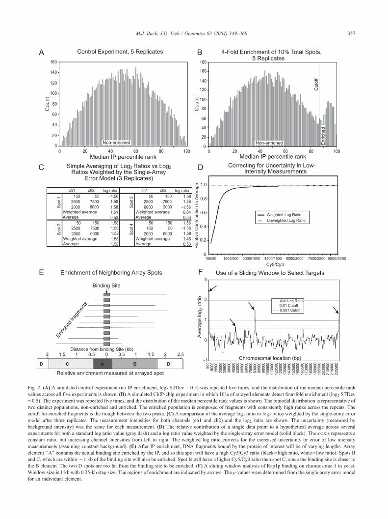
Fig. 2. (A) A simulated control experiment (no IP enrichment, log2 STDev = 0.5) was repeated five times, and the distribution of the median percentile rank

values across all five experiments is shown. (B) A simulated ChIP-chip experiment in which 10% of arrayed elements detect four-fold enrichment (log2 STDev

= 0.5). The experiment was repeated five times, and the distribution of the median percentile rank values is shown. The bimodal distribution is representative of

two distinct populations, non-enriched and enriched. The enriched population is composed of fragments with consistently high ranks across the repeats. The

cutoff for enriched fragments is the trough between the two peaks. (C) A comparison of the average log2 ratio to log2 ratios weighted by the single-array error

model after three replicates. The measurement intensities for both channels (ch1 and ch2) and the log2 ratio are shown. The uncertainty (measured by

background intensity) was the same for each measurement. (D) The relative contribution of a single data point to a hypothetical average across several

experiments for both a standard log ratio value (gray dash) and a log ratio value weighted by the single-array error model (solid black). The x-axis represents a

constant ratio, but increasing channel intensities from left to right. The weighted log ratio corrects for the increased uncertainty or error of low intensity

measurements (assuming constant background). (E) After IP enrichment, DNA fragments bound by the protein of interest will be of varying lengths. Array

element ‘‘A’’ contains the actual binding site enriched by the IP, and so this spot will have a high Cy5/Cy3 ratio (black=high ratio, white= low ratio). Spots B

and C, which are withinf1 kb of the binding site will also be enriched. Spot B will have a higher Cy5/Cy3 ratio then spot C, since the binding site is closer to

the B element. The two D spots are too far from the binding site to be enriched. (F) A sliding window analysis of Rap1p binding on chromosome 1 in yeast.

Window size is 1 kb with 0.25-kb step size. The regions of enrichment are indicated by arrows. The p-values were determined from the single-array error model

for an individual element.

M.J. Buck, J.D. Lieb / Genomics 83 (2004) 349–360 357

enomics 83 (2004) 349–360

A sliding-window approach

In contrast to mRNA microarray experiments, in which

each arrayed element usually measures the abundance of one

mRNA species, in ChIP-chip experiments each element

measures the abundance of a population of fragments of

assorted lengths due to chromatin shearing (Fig. 2E). There-

fore, arrayed elements representing genomic regions 1 to 2

kb downstream or upstream of the binding site will also

detect enrichment. This effect produces a peak over several

arrayed elements containing genomically adjacent DNA.

This is nonrandom behavior that is not expected from

spuriously high ratio measurements. One can take advantage

of this fact and use it as an independent confirmation of

enrichment for a given genomic region.

When using tiled arrays containing short DNA frag-

ments, several neighboring genomic elements will identify

each protein–DNA interaction. If chromatin is sheared

randomly to an average size of 1 kb in a ChIP experiment,

at least a 2-kb region of the genome surrounding the actual

site of protein–DNA interaction will be enriched. To take

advantage of this unique property of ChIP-chip experiments,

a simple but powerful sliding-window approach has been

developed to characterize binding sites for transcription

factors when using full-genome arrays in yeast (Fig. 2F).

With this approach, a window of 1 kb is slid across a region

or chromosome, and the average log2 ratio of any arrayed

elements that fall within that window is determined. The

window is moved downstream 0.25 kb, and then the

calculation is repeated iteratively for the entire length of

chromosome. This sliding average will identify binding sites

as peaks. The height of peaks caused by spuriously high

ratios will be reduced, since the probability of a neighboring

genomic element also having a high ratio is extremely low.

In addition, a confidence value for each peak can be

assigned based on the number of independent arrayed

elements used to construct the peak. The utility of this

approach does not depend on the absolute number of

targets, but on the density of their distribution. It is

appropriate for detecting any number of targets that are

distributed with a frequency less than approximately three

times the average sheared chromatin size. For example, if

the average sheared chromatin size were 1 kb, this method

would be useful for the detection of any protein predicted

to be spaced at intervals of at least 3 kb. A drawback to

this approach is that it requires high-resolution tiling

arrays.

M.J. Buck, J.D. Lieb / G358

Future applications and challenges

Arrays designed specifically for the ChIP-chip technique

should be developed and utilized. Ideally, arrays should be

designed with short DNA fragments (f0.5 kb) of equal

lengths that are tiled for continuous genomic regions (short

element tiling, or SET, arrays). Use of SET arrays with

ChIP-chip experiments derived from sheared chromatin of

f1 kb should allow for enrichment of the binding site and

at least two neighboring regions, which can be used to

confirm the core binding location. The ratio between the

log2 ratios for the upstream and downstream regions should

be proportional to the distance from the center of the

binding site. In theory, this would allow the center of

binding to be predicted, to the base pair, from the raw data

(Fig. 2E).

Aside from technical advances, which will undoubtedly

allow more accurate and precise determinations of DNA–

protein interactions, simply incorporating ChIP-chip experi-

ments into the standard molecular biology toolbox will

result in a flood of functional data. Time-course experiments

to determine binding order, recruitment relationships, and

codependencies have already been carried out [17]. While

most experiments to date have been performed in culture on

cell lines, bacteria, or yeast, future experiments will include

ChIPs from developing tissues, organs, or cancer biopsies

[54]. Across all of biology, the ChIP-chip platform will be

critical in elucidating the function of genomes and the

proteins they encode.

References

[1] J.D. Lieb, X. Liu, D. Botstein, P.O. Brown, Promoter-specific binding

of Rap1 revealed by genome-wide maps of protein–DNA association,

Nat. Genet. 28 (2001) 327–334.

[2] A. Wagner, Estimating coarse gene network structure from large-scale

gene perturbation data, Genome Res. 12 (2002) 309–315.

[3] T.R. Hughes, M.J. Marton, A.R. Jones, C.J. Roberts, R. Stoughton,

C.D. Armour, H.A. Bennett, E. Coffey, H. Dai, Y.D. He, M.J. Kidd,

A.M. King, M.R. Meyer, D. Slade, P.Y. Lum, S.B. Stepaniants, D.D.

Shoemaker, D. Gachotte, K. Chakraburtty, J. Simon, M. Bard, S.H.

Friend, Functional discovery via a compendium of expression pro-

files, Cell 102 (2000) 109–126.

[4] K.D. Johnson, E.H. Bresnick, Dissecting long-range transcriptional

mechanisms by chromatin immunoprecipitation, Methods 26 (2002)

27–36.

[5] M.H. Kuo, C.D. Allis, In vivo cross-linking and immunoprecipitation

for studying dynamic protein:DNA associations in a chromatin envi-

ronment, Methods 19 (1999) 425–433.

[6] S.K. Kurdistani, M. Grunstein, In vivo protein–protein and protein–

DNA crosslinking for genomewide binding microarray, Methods 31

(2003) 90–95.

[7] B. Nal, E. Mohr, P. Ferrier, Location analysis of DNA-bound proteins

at the whole-genome level: untangling transcriptional regulatory net-

works, Bioessays 23 (2001) 473–476.

[8] V. Orlando, Mapping chromosomal proteins in vivo by formaldehyde-

crosslinked-chromatin immunoprecipitation, Trends Biochem. Sci. 25

(2000) 99–104.

[9] D. Robyr, M. Grunstein, Genomewide histone acetylation microar-

rays, Methods 31 (2003) 83–89.

[10] V.A. Spencer, J.M. Sun, L. Li, J.R. Davie, Chromatin immunopreci-

pitation: a tool for studying histone acetylation and transcription fac-

tor binding, Methods 31 (2003) 67–75.

[11] A.S. Weinmann, P.J. Farnham, Identification of unknown target genes

of human transcription factors using chromatin immunoprecipitation,

Methods 26 (2002) 37–47.

[12] J. Wells, P.J. Farnham, Characterizing transcription factor binding

sites using formaldehyde crosslinking and immunoprecipitation,

Methods 26 (2002) 48–56.

M.J. Buck, J.D. Lieb / Genomics 83 (2004) 349–360 359

[13] J.D. Lieb, Genome-wide mapping of protein–DNA interactions by

chromatin immunoprecipitation and DNA microarray hybridization,

Methods Mol. Biol. 224 (2003) 99–109.

[14] S.K. Kurdistani, D. Robyr, S. Tavazoie, M. Grunstein, Genome-wide

binding map of the histone deacetylase Rpd3 in yeast, Nat. Genet. 31

(2002) 248–254.

[15] V.R. Iyer, C.E. Horak, C.S. Scafe, D. Botstein, M. Snyder, P.O.

Brown, Genomic binding sites of the yeast cell-cycle transcription

factors SBF and MBF, Nature 409 (2001) 533–538.

[16] B. Ren, F. Robert, J.J. Wyrick, O. Aparicio, E.G. Jennings, I. Simon,

J. Zeitlinger, J. Schreiber, N. Hannett, E. Kanin, T.L. Volkert, C.J.

Wilson, S.P. Bell, R.A. Young, Genome-wide location and function

of DNA binding proteins, Science 290 (2000) 2306–2309.

[17] T.I. Lee, N.J. Rinaldi, F. Robert, D.T. Odom, Z. Bar-Joseph, G.K.

Gerber, N.M. Hannett, C.T. Harbison, C.M. Thompson, I. Simon, J.

Zeitlinger, E.G. Jennings, H.L. Murray, D.B. Gordon, B. Ren, J.J.

Wyrick, J.B. Tagne, T.L. Volkert, E. Fraenkel, D.K. Gifford, R.A.

Young, Transcriptional regulatory networks in Saccharomyces cere-

visiae, Science 298 (2002) 799–804.

[18] Z. Li, S. Van Calcar, C. Qu, W.K. Cavenee, M.Q. Zhang, B. Ren, A

global transcriptional regulatory role for c-Myc in Burkitt’s lympho-

ma cells, Proc. Natl. Acad. Sci. USA 100 (2003) 8164–8169.

[19] C.E. Horak, N.M. Luscombe, J. Qian, P. Bertone, S. Piccirrillo, M.

Gerstein, M. Snyder, Complex transcriptional circuitry at the G1/S

transition in Saccharomyces cerevisiae, Genes Dev. 16 (2002)

3017–3033.

[20] C.E. Horak, M.C. Mahajan, N.M. Luscombe, M. Gerstein, S.M.

Weissman, M. Snyder, GATA-1 binding sites mapped in the beta-

globin locus by using mammalian chIp-chip analysis, Proc. Natl.

Acad. Sci. USA 99 (2002) 2924–2929.

[21] A.S. Weinmann, P.S. Yan, M.J. Oberley, T.H. Huang, P.J. Farnham,

Isolating human transcription factor targets by coupling chromatin

immunoprecipitation and CpG island microarray analysis, Genes

Dev. 16 (2002) 235–244.

[22] J. Wells, P.S. Yan, M. Cechvala, T. Huang, P.J. Farnham, Identifica-

tion of novel pRb binding sites using CpG microarrays suggests that

E2F recruits pRb to specific genomic sites during S phase, Oncogene

22 (2003) 1445–1460.

[23] P.L. Nagy, M.L. Cleary, P.O. Brown, J.D. Lieb, Genomewide demar-

cation of RNA polymerase II transcription units revealed by physical

fractionation of chromatin, Proc. Natl. Acad. Sci. USA 100 (2003)

6364–6369.

[24] B.E. Bernstein, E.L. Humphrey, R.L. Erlich, R. Schneider, P. Bou-

man, J.S. Liu, T. Kouzarides, S.L. Schreiber, Methylation of histone

H3 Lys 4 in coding regions of active genes, Proc. Natl. Acad. Sci.

USA 99 (2002) 8695–8700.

[25] H.H. Ng, F. Robert, R.A. Young, K. Struhl, Genome-wide location

and regulated recruitment of the RSC nucleosome-remodeling com-

plex, Genes Dev. 16 (2002) 806–819.

[26] O. Puig, F. Caspary, G. Rigaut, B. Rutz, E. Bouveret, E. Bragado-

Nilsson, M. Wilm, B. Seraphin, The tandem affinity purification

(TAP) method: a general procedure of protein complex purification,

Methods 24 (2001) 218–229.

[27] S.K. Bohlander, R. Espinosa III, M.M. Le Beau, J.D. Rowley,

M.O. Diaz, A method for the rapid sequence-independent amplifica-

tion of microdissected chromosomal material, Genomics 13 (1992)

1322–1324.

[28] P.R. Mueller, B. Wold, In vivo footprinting of a muscle specific

enhancer by ligation mediated PCR, Science 246 (1989) 780–786.

[29] C.L. Liu, S.L. Schreiber, B.E. Bernstein, Development and validation

of a T7 based linear amplification for genomic DNA, BMC Genom. 4

(2003) 19.

[30] D.J. Duggan, M. Bittner, Y. Chen, P. Meltzer, J.M. Trent, Expres-

sion profiling using cDNA microarrays, Nat. Genet. 21 (1999)

10–14.

[31] C.C. Xiang, O.A. Kozhich, M. Chen, J.M. Inman, Q.N. Phan,

Y. Chen, M.J. Brownstein, Amine-modified random primers to

label probes for DNA microarrays, Nat. Biotechnol. 20 (2002)

738–742.

[32] X.S. Liu, D.L. Brutlag, J.S. Liu, An algorithm for finding protein–

DNA binding sites with applications to chromatin-immunoprecipita-

tion microarray experiments, Nat. Biotechnol. 20 (2002) 835–839.

[33] X. Liu, D.L. Brutlag, J.S. Liu, BioProspector: discovering conserved

DNA motifs in upstream regulatory regions of co-expressed genes,

Pac. Symp. (2001) 127–138.

[34] J.J. Wyrick, J.G. Aparicio, T. Chen, J.D. Barnett, E.G. Jennings, R.A.

Young, S.P. Bell, O.M. Aparicio, Genome-wide distribution of ORC

and MCM proteins in S. cerevisiae: high-resolution mapping of rep-

lication origins, Science 294 (2001) 2357–2360.

[35] J.L. Gerton, J. DeRisi, R. Shroff, M. Lichten, P.O. Brown, T.D. Petes,

Inaugural article: global mapping of meiotic recombination hotspots

and coldspots in the yeast Saccharomyces cerevisiae, Proc. Natl.

Acad. Sci. USA 97 (2000) 11383–11390.

[36] D. Robyr, Y. Suka, I. Xenarios, S.K. Kurdistani, A. Wang, N. Suka, M.

Grunstein, Microarray deacetylation maps determine genome-wide

functions for yeast histone deacetylases, Cell 109 (2002) 437–446.

[37] F. Antequera, A. Bird, Number of CpG islands and genes in human

and mouse, Proc. Natl. Acad. Sci. USA 90 (1993) 11995–11999.

[38] S.H. Cross, J.A. Charlton, X. Nan, A.P. Bird, Purification of CpG

islands using a methylated DNA binding column, Nat. Genet. 6

(1994) 236–244.

[39] Y. Moreau, S. Aerts, B. De Moor, B. De Strooper, M. Dabrowski,

Comparison and meta-analysis of microarray data: from the bench to

the computer desk, Trends Genet. 19 (2003) 570–577.

[40] Y.F. Leung, D. Cavalieri, Fundamentals of cDNA microarray data

analysis, Trends Genet. 19 (2003) 649–659.

[41] J. Quackenbush, Microarray data normalization and transformation,

Nat. Genet. 32 Suppl. (2002) 496–501.

[42] Y.D. He, H. Dai, E.E. Schadt, G. Cavet, S.W. Edwards, S.B. Stepa-

niants, S. Duenwald, R. Kleinhanz, A.R. Jones, D.D. Shoemaker,

R.B. Stoughton, Microarray standard data set and figures of merit

for comparing data processing methods and experiment designs, Bio-

informatics 19 (2003) 956–965.

[43] N. Kaminski, N. Friedman, Practical approaches to analyzing results

of microarray experiments, Am. J. Respir. Cell Mol. Biol. 27 (2002)

125–132.

[44] J.L. Rinn, G. Euskirchen, P. Bertone, R. Martone, N.M. Luscombe, S.

Hartman, P.M. Harrison, F.K. Nelson, P. Miller, M. Gerstein, S.

Weissman, M. Snyder, The transcriptional activity of human chromo-

some 22, Genes Dev. 17 (2003) 529–540.

[45] P. Kapranov, S.E. Cawley, J. Drenkow, S. Bekiranov, R.L. Strausberg,

S.P. Fodor, T.R. Gingeras, Large-scale transcriptional activity in chro-

mosomes 21 and 22, Science 296 (2002) 916–919.

[46] A.M. Snijders, N. Nowak, R. Segraves, S. Blackwood, N. Brown,

J. Conroy, G. Hamilton, A.K. Hindle, B. Huey, K. Kimura, S. Law,

K. Myambo, J. Palmer, B. Ylstra, J.P. Yue, J.W. Gray, A.N. Jain,

D. Pinkel, D.G. Albertson, Assembly of microarrays for genome-

wide measurement of DNA copy number, Nat. Genet. 29 (2001)

263–264.

[47] E.F. Nuwaysir, W. Huang, T.J. Albert, J. Singh, K. Nuwaysir, A. Pitas,

T. Richmond, T. Gorski, J.P. Berg, J. Ballin, M. McCormick, J. Nor-

ton, T. Pollock, T. Sumwalt, L. Butcher, D. Porter, M. Molla, C. Hall,

F. Blattner, M.R. Sussman, R.L. Wallace, F. Cerrina, R.D. Green,

Gene expression analysis using oligonucleotide arrays produced by

maskless photolithography, Genome Res. 12 (2002) 1749–1755.

[48] S. Brenner, M. Johnson, J. Bridgham, G. Golda, D.H. Lloyd, D.

Johnson, S. Luo, S. McCurdy, M. Foy, M. Ewan, R. Roth, D. George,

S. Eletr, G. Albrecht, E. Vermaas, S.R. Williams, K. Moon, T. Bur-

cham, M. Pallas, R.B. DuBridge, J. Kirchner, K. Fearon, J. Mao, K.

Corcoran, Gene expression analysis by massively parallel signature

sequencing (MPSS) on microbead arrays, Nat. Biotechnol. 18 (2000)

630–634.

[49] C.Workman, L.J. Jensen, H. Jarmer, R. Berka, L. Gautier, H.B. Nielser,

H.H. Saxild, C. Nielsen, S. Brunak, S. Knudsen, A new non-linear

M.J. Buck, J.D. Lieb / Genomics 83 (2004) 349–360360

normalization method for reducing variability in DNA microarray ex-

periments, Genome Biol. 3 (2002) (research 0048.1–0048.16).

[50] Y.H. Yang, S. Dudoit, P. Luu, D.M. Lin, V. Peng, J. Ngai, T.P. Speed,

Normalization for cDNA microarray data: a robust composite method

addressing single and multiple slide systematic variation, Nucleic

Acids Res. 30 (2002) e15.

[51] G.C. Tseng, M.K. Oh, L. Rohlin, J.C. Liao, W.H. Wong, Issues in

cDNA microarray analysis: quality filtering, channel normalization,

models of variations and assessment of gene effects, Nucleic Acids

Res. 29 (2001) 2549–2557.

[52] E.E. Schadt, C. Li, B. Ellis, W.H. Wong, Feature extraction and

normalization algorithms for high-density oligonucleotide gene ex-

pression array data, J. Cell. Biochem. Suppl. Suppl. 37 (2001)

120–125.

[53] C.J. Roberts, B. Nelson, M.J. Marton, R. Stoughton, M.R. Meyer,

H.A. Bennett, Y.D. He, H. Dai, W.L. Walker, T.R. Hughes, M. Tyers,

C. Boone, S.H. Friend, Signaling and circuitry of multiple MAPK

pathways revealed by a matrix of global gene expression profiles,

Science 287 (2000) 873–880.

[54] E.C. Forsberg, K.M. Downs, E.H. Bresnick, Direct interaction of NF-

E2 with hypersensitive site 2 of the beta-globin locus control region in

living cells, Blood 96 (2000) 334–339.