CHIRON efficiency tests

Julien Spronck, Christian Schwab

June 15, 2011

In this document, we report the tests that have been performed on CHIRON in order to understandits efficiency.

1 Fiber throughput and FRD measurement

We have injected a HeNe laser at 543 nm into the science fiber. A set of lenses and a diaphragm (incollimated space) were used after the laser to inject the beam with the correct focal ratio. The diameterof the diaphragm was set to 4 mm, while the focal length of the focusing lens was 19 mm, which givesan input focal ratio (IFR) of F/4.75.

After aligning the fiber in x, y and z directions, we measured the power after and before the fiber,

Pbefore = 935 ± 10µW and Pafter = 835± 10µW, (1)

which gives a transmission of 89 ± 2%.In order to measure the focal ratio after the fiber, we have plugged the fiber into a connector and then

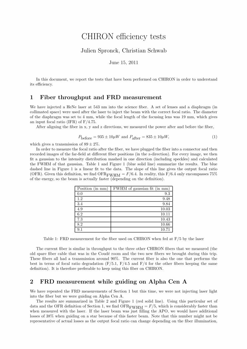
recorded images of the far-field at different fiber positions (in the z-direction). For every image, we thenfit a gaussian to the intensity distribution mashed in one direction (including speckles) and calculatedthe FWHM of that gaussian. Table 1 and Figure 1 (blue solid line) summarize the results. The bluedashed line in Figure 1 is a linear fit to the data. The slope of this line gives the output focal ratio(OFR). Given this definition, we find OFRFWHM = F/6.4. In reality, this F/6.4 only encompasses 75%of the energy, so the beam is actually faster (depending on the definition).

Position (in mm) FWHM of gaussian fit (in mm)0.0 9.31.2 9.483.4 9.844.9 10.036.2 10.117.3 10.438.2 10.669.1 10.71

Table 1: FRD measurement for the fiber used on CHIRON when fed at F/5 by the laser

The current fiber is similar in throughput to the three other CHIRON fibers that we measured (theold spare fiber cable that was in the Coude room and the two new fibers we brought during this trip.These fibers all had a transmission around 90%. The current fiber is also the one that performs thebest in terms of focal ratio degradation (F/5.1, F/4.5 and F/4 for the other fibers keeping the samedefinition). It is therefore preferable to keep using this fiber on CHIRON.

2 FRD measurement while guiding on Alpha Cen A

We have repeated the FRD measurements of Section 1 but this time, we were not injecting laser lightinto the fiber but we were guiding on Alpha Cen A.

The results are summarized in Table 2 and Figure 1 (red solid line). Using this particular set ofdata and the OFR definition of Section 1, we find OFRFWHM = F/5, which is considerably faster thanwhen measured with the laser. If the laser beam was just filling the APO, we would have additionallosses of 38% when guiding on a star because of this faster beam. Note that this number might not berepresentative of actual losses as the output focal ratio can change depending on the fiber illumination,

0 5 10 15

Position of the fiber (in mm)

9.5

10.0

10.5

11.0

11.5

12.0

FW

HM

of

ga

uss

ian

fit

(in

mm

)

Figure 1: Output focal ratio of the science fiber when fed at with a laser at F/4.75 (blue solid line) andwhen guiding on Alpha Cen A (red solid line). The blue and red dashed lines are linear fits to the data.

hence depending on guiding. This is especially true if the guiding system allows the light to reach thecladding of the fiber, which can happen if there is a slight misalignment between the hole used for guidingand the fiber itself.

This might be the cause of significant losses.

Position (in mm) FWHM of gaussian fit (in mm)0.0 9.27.3 10.610.75 11.413.3 11.814.9 12.1

Table 2: FRD measurement for the fiber used on CHIRON when guiding on Alpha Cen A

3 Spectrograph throughput

Using the laser feeding the science fiber at F/5, we plugged the fiber back into CHIRON and looked atthe beam and the light path to see potential sources of loss.

3.1 Visual inspection

We have seen possible vignetting by the shutter but it could be a back-reflection that we see.The iodine cell did not seem to vignet the beam further. However, the iodine cell motor failed to

work and the cell needed to be pushed manually.After the CFA, we noticed an odd shape (a little glitch in the round distribution), indicating possible

vignetting (though very small). This might be present before the CFA, but the beam was too small toclearly see it.

The beam seems well centered on the collimator. It is slightly overfilling the collimator (by a fewmm).

The beam on the collimator seems vignetted. It seemed to be due to L1. The bean on L1 seemedhighly eccentric, but the current fiber holder does not allow to correct it, as we are limited in the numberof degrees of freedom for the spectrograph alignment. Adding a tilt stage for the fiber should help.

3.2 Throughput measurement

Using the same laser and fiber feed, we have measured the power at different positions in the spectrographusing our power meter. We measured the power after L1, before the CFA, after the CFA and finallybefore the field flattener. The laser line seemed to fall onto the edge of the free spectral range (FSR)of the CCD, so we could see two distinct spots in the focal plane (and two additional spots outside theFSR). The power of these two spots were measured separately and then combined to yield the totalpower of the beam. Since the beam before the field flattener is much larger than the photodiode we usedfor the measurement, we needed to install a flat mirror to redirect the light where we could access thefocus.

Table 3 summarizes our measurements. The spectrograph throughput should be given by the sum ofthe power of the two orders divided by the power before the CFA. This yields a spectrograph throughputof (128 + 183)/803 = 38%, which is very close to the throughput calculated by A. Tokovinin in his effi-ciency report of March 28, 2011. In this report, a spectrograph throughput of 39% was found (excludingfield flattener, L1 and L2). However, vignetting was not taken into account, since the measurementswere done with a narrow beam. A lower throughput with a large beam was expected but not measured.This also shows that the possible loss candidates mentioned in Section 3.1 are negligible.

Power (in µW) (Meas. 1) Power (in µW) (Meas. 2) ± (in µW) Position800 820 20 After L1805 800 10 Before CFA760 770 20 After CFA128 128 3 Bottom order183 183 3 Top order16 17 2 Sec. order (top)12 12 2 Sec. order (bottom)1.9 Line bet. spots

Table 3: Measurements of the spectrograph throughput.

4 Efficiency of the slicer and slits

Using the laser feeding the fiber at f/5, we have measured the relative efficiencies of the different observingmodes by placing a power meter in front of the field flattener (with the help of a flat mirror). Table 4summarizes the results. We see that the slicer efficiency is much lower than expected. This efficiencycannot be taken into account only by the blocking of he fourth slice. It could be the mirror coatings,scattering on the slicing edge and/or vignetting by the shutter edge. Most likely, it is a combination ofall these effects.

Fiber (in µW) Slicer (in µW) Slit (in µW) Narrow Slit (in µW)168.5 ± 2 100 ± 2 49.7 ± 0.5 24.2 ± 0.3

1.0 0.59 0.29 0.14

172.2 ± 2 101.9 ± 1 49.7 ± 0.4 25.3 ± 0.51.0 0.59 0.29 0.15

Table 4: Efficiency of the slicer and of the slits.

5 Quantum efficiency of the detector

We estimated the quantum efficiency of the CCD in two different ways.First we installed a diaphragm in front of the field flattener. We used the quartz lamp injected in the

fiber that feeds CHIRON. We measured the power directly after the diaphragm with the power meterand then recorded a spectrum with the CCD using the same diaphragm. We subtracted the bias, countedall counts incident on each amplifier and multiplied by their respective gain to get the total number ofphotons on each side of the CCD. We added these to get the total number of photons.

Nph = g1 ∗ C1 + g2 ∗ C2, (2)

where g1, g2 are the gains and C1, C2 are the number of counts corresponding to both CCD amplifiers.To get the energy corresponding these photons, we assumed that they were all at a wavelength ofλ = 550 nm. We have

Eph =Nphhc

λ, (3)

where h is Planck constant and c is the speed of light. We then divide by the exposure time to find thepower. We find a power of 24.9 pW.

In the second measurement, we have used the quartz lamp and a green filter going from 500 to600 nm. We then measured the power right after the fiber and the power on the CCD (the same way wedid it in the first measurement).

Table 5 summarizes the results. The quantum efficiency was calculated by dividing the power on thepower meter by the power on the ccd. Additionally, we divided it in the first case by the efficiency ofthe field flattener (0.98) and in the second case by the measured efficiency of the spectrograph (0.38 ∗

0.98 ∗ 0.98 = 0.36).The measurements are probably not very precise but they are in agreement with the vendor data

(85%). We then conclude that the quantum efficiency is not responsible for the bad efficiency that wehave with CHIRON.

Power meter Power on CCD QE Comments28 pW 24.9 pW 90% First meas., QE = 24.9/28./0.98 (field flattener)4.78 nW 1.38 nW 80% Sec. meas., QE = 1.38/4.78/0.36 (spectrograph)

Table 5: Efficiency of the slicer and of the slits.

6 Power measurement while guiding on Alpha Cen A

Using our power meter positioned right after the fiber and the green (500-600 nm) filter, we have recordedthe power coming from Alpha Cen A as a function of time for a period of three hours (see Figure 2, onlyone hour is depicted).

The first thing to notice is how wild the power variations are. Over the three hours of data (only onehour is depicted in Figure 2), the power varied between 50 and 475 pW with an average at 221 pW. Themaximum power of 475 pW is unexpectedly low. From previous calculations (see J. Spronck’s documenton Exposure Meter Photometry of May 11, 2011), we expected to have a power of 1.7 nW behind thefiber, which is 3.5 times more than the maximum value measured during this lapse of time. Possibleexplanations for this could be:

• Bad weather conditions: it was clear upon visual inspection, the seeing was reported to be good(0.75 on the Tololo weather page) but it was rather windy;

• Guiding losses: the large power variations might indicate important guiding losses. Can there beadditional guiding losses up to a factor 3.5?

• Misalignment of the FEM: we have aligned the FEM as well as we could. The fiber image throughthe FEM viewer seemed round and centered. However, there is no focus adjustment in the FEM.Is it possible that the components have shifted in the z-direction?

• Error in the power estimate from a zero-th magnitude star: that could be possible and would alsoexplain where our throughput disappeared; We actually figured out that there is a mistake

in the calculation. The collecting area of the telescope was counted to be 1.77 m2. This

does not include the obstruction from the secondary mirror though, which is 0.76 m

in diameter. This would bring the collecting area down from 1.77 m2 to 1.31 m2 and

the expected power from a zeroth magnitude star from 1.7 nW to 1.26 nW. The same

mistake seems to be present in the document on CHIRON efficiency of March 28,

2011.

• Power meter is not calibrated: possible.

Even if we could explain this factor 3.5, the average power is still twice lower than the maximumpower. This additional factor is probably due to guiding/tracking errors. Indeed, we see in Figure 3 thepower spectral density of the signal depicted in Figure 2. We clearly see a peak in the power spectral

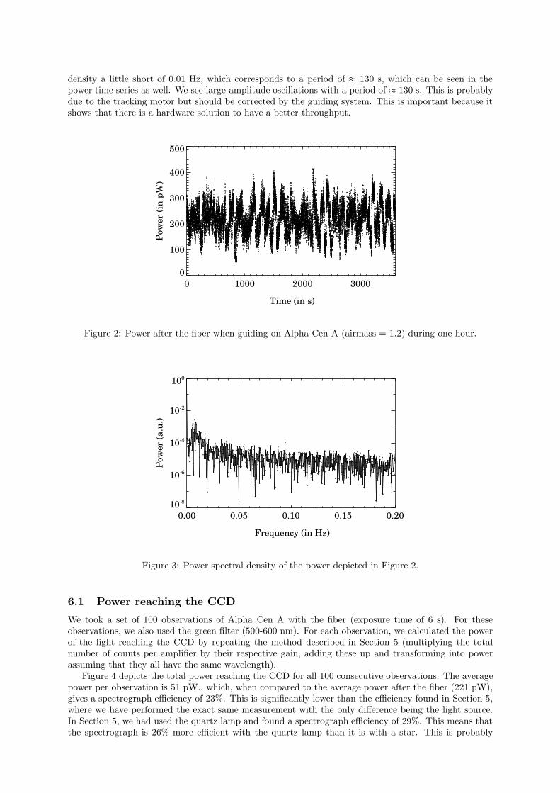
density a little short of 0.01 Hz, which corresponds to a period of ≈ 130 s, which can be seen in thepower time series as well. We see large-amplitude oscillations with a period of ≈ 130 s. This is probablydue to the tracking motor but should be corrected by the guiding system. This is important because itshows that there is a hardware solution to have a better throughput.

0 1000 2000 3000

Time (in s)

0

100

200

300

400

500P

ow

er

(in

pW

)

Figure 2: Power after the fiber when guiding on Alpha Cen A (airmass = 1.2) during one hour.

0.00 0.05 0.10 0.15 0.20

Frequency (in Hz)

10-8

10-6

10-4

10-2

100

Pow

er

(a.u

.)

Figure 3: Power spectral density of the power depicted in Figure 2.

6.1 Power reaching the CCD

We took a set of 100 observations of Alpha Cen A with the fiber (exposure time of 6 s). For theseobservations, we also used the green filter (500-600 nm). For each observation, we calculated the powerof the light reaching the CCD by repeating the method described in Section 5 (multiplying the totalnumber of counts per amplifier by their respective gain, adding these up and transforming into powerassuming that they all have the same wavelength).

Figure 4 depicts the total power reaching the CCD for all 100 consecutive observations. The averagepower per observation is 51 pW., which, when compared to the average power after the fiber (221 pW),gives a spectrograph efficiency of 23%. This is significantly lower than the efficiency found in Section 5,where we have performed the exact same measurement with the only difference being the light source.In Section 5, we had used the quartz lamp and found a spectrograph efficiency of 29%. This means thatthe spectrograph is 26% more efficient with the quartz lamp than it is with a star. This is probably

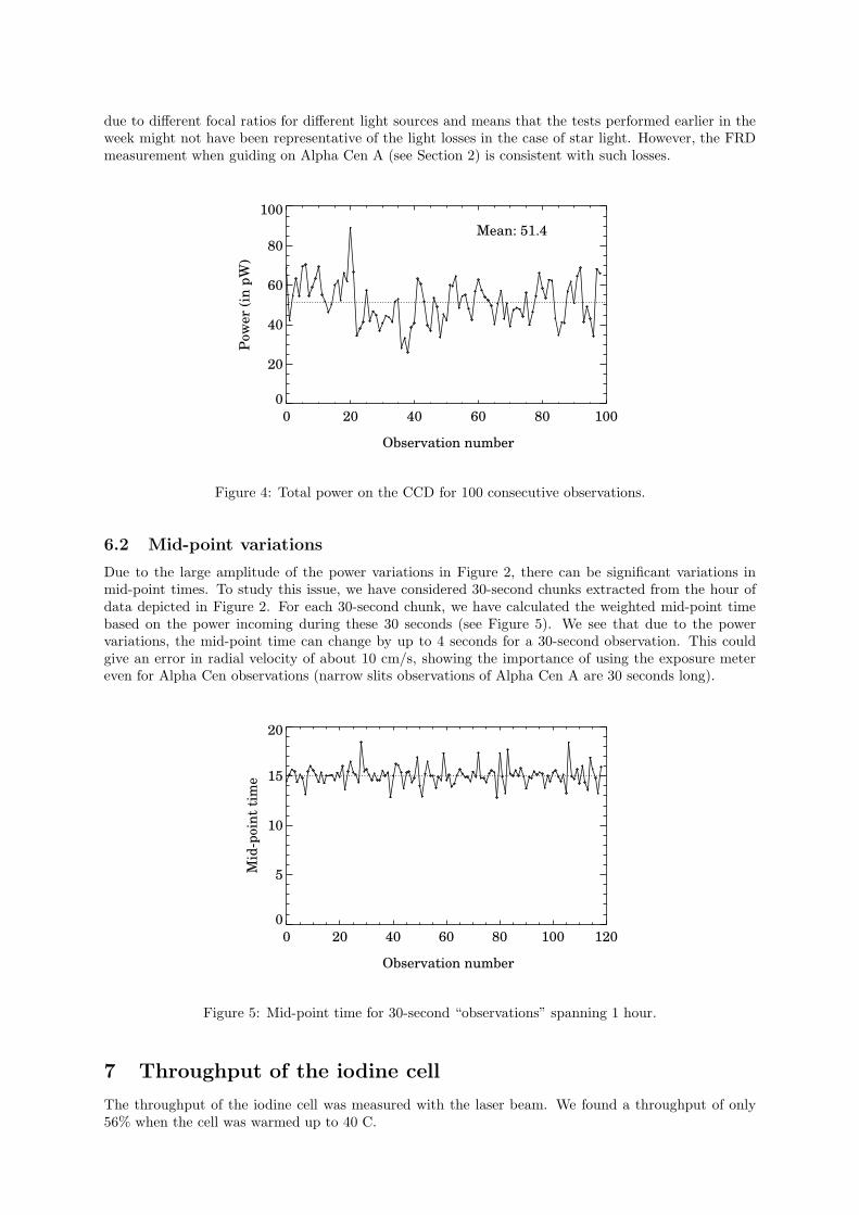
due to different focal ratios for different light sources and means that the tests performed earlier in theweek might not have been representative of the light losses in the case of star light. However, the FRDmeasurement when guiding on Alpha Cen A (see Section 2) is consistent with such losses.

0 20 40 60 80 100

Observation number

0

20

40

60

80

100

Pow

er

(in

pW

)Mean: 51.4

Figure 4: Total power on the CCD for 100 consecutive observations.

6.2 Mid-point variations

Due to the large amplitude of the power variations in Figure 2, there can be significant variations inmid-point times. To study this issue, we have considered 30-second chunks extracted from the hour ofdata depicted in Figure 2. For each 30-second chunk, we have calculated the weighted mid-point timebased on the power incoming during these 30 seconds (see Figure 5). We see that due to the powervariations, the mid-point time can change by up to 4 seconds for a 30-second observation. This couldgive an error in radial velocity of about 10 cm/s, showing the importance of using the exposure metereven for Alpha Cen observations (narrow slits observations of Alpha Cen A are 30 seconds long).

0 20 40 60 80 100 120

Observation number

0

5

10

15

20

Mid

-poin

t ti

me

Figure 5: Mid-point time for 30-second “observations” spanning 1 hour.

7 Throughput of the iodine cell

The throughput of the iodine cell was measured with the laser beam. We found a throughput of only56% when the cell was warmed up to 40 C.

8 Comparison with previous observations

We have run the program getpowerccd.pro on all Alpha Cen A observations in April and May. Thisprograms returns the total power reaching the CCD (between 500 and 600 nm) for a given observation.

Figure 6 depicts the power for all Alpha Cen A observations since April 1st, 2011. All these observa-tions have iodine. First thing to notice is that the power varies by a large amount, which is consistentwith the measurements of Section 6. These large variations are probably due to weather changes, seeingvariations and guiding/tracking errors.

In order to estimate the overall efficiency of the spectrograph, we need to know how much lightto expect from Alpha Cen A above the atmosphere. According to Oke and Schild, 1970 (The Ab-solute Spectral Energy Distribution of Alpha Lyrae) and Schild et al., 1971, Alpha Lyrae radiates3.64 10−8 J/m2/s/µm (of wavelength) above the atmosphere of the Earth at a wavelength of 0.548 µm.The band-pass filter that we will use in front of the PMT has a FWHM of ≈ 80 nm, which givesE = 2.9 10−9 J/m2/s. For a 1.5 m telescope with a 76 cm central obstruction (area = 1.31 m2), wehave P = 3.8 10−9 W = 3.8 nW . This is the power captured by the 1.5-m telescope in a 80-nm band

for a 0th magnitude star above the atmosphere.Using this number and the numbers that we measured in Section 7 for the iodine cell throughput

and in Section 4 for the efficiency of the slicer and the narrow slit, we can plot the overall spectrographefficiency (from atmosphere to detector) as a function of time (see Figure 7). The fact that the blue andred curve overlap well is a sign that variations are mainly due to weather conditions. The fluctuationswithin a night can also be weather/seeing related but are most likely due to guiding/tracking errors. Wesee that the overall spectrograph efficiency tops at 11−12%, indicating that there is nothing wrong withthe spectrograph efficiency. And that the previously calculated efficiency was simply underestimated.

However, the weather/guiding averaged efficiency is closer to 8%. There is not much we can do aboutthe weather but guiding could be improved if we need to get higher efficiencies.

The other thing to note is that the efficiency dropped considerably the two days after our visit (June12 and 13), indicating some misalignment that should be fixed. A longer baseline is needed to see whetherthis lower efficiency is not weather related. However, in the last two months, there is no history of sucha low throughput for two days in a row.

0 20 40 60 80

JD (0 = Apr 1, 2011)

0

50

100

150

Pow

er

on

CC

D (

50

0-6

00

nm

) (i

n p

W)

Figure 6: Power reaching the CCD for all Alpha Cen A observations since April 1st, 2011. Red trianglesand blue diamond correspond respectively to narrow slit and slicer observations.

9 Conclusions

We have thoroughly tested the efficiency of the spectrograph and have found a few interesting things:

• The fiber currently used on CHIRON was measured to be the best fiber in terms of FRD and asgood as other fibers in terms of transmission.

0 20 40 60 80

JD (0 = Apr 1, 2011)

0.00

0.02

0.04

0.06

0.08

0.10

0.12

Tota

l S

pect

rogra

ph

Eff

icie

ncy

Figure 7: Overall spectrograph efficiency since April 1st, 2011. Red triangles and blue diamond corre-spond respectively to narrow slit and slicer observations.

• The FRD was worse than expected when guiding on Alpha Cen A, probably yielding 26% losseswhen compared to the efficiency measured with the quartz lamp.

• The quantum efficiency of the detector was measured to be as expected (80 − 90%).

• The slicer has an unacceptably low throughput of 59%.

• The iodine cell when warmed at 40 C has a throughput of only 56%.

• We found large amplitude power variations coming from the star, with a clear period at ≈ 130 s.There should be a hardware solution to minimize this effect.

• These large amplitude power fluctuations make the use of an exposure meter necessary even forAlpha Cen observations.

• The previous value measured for the spectrograph efficiency seemed underestimated. The peakoverall spectrograph efficiency was calculated to be as high as expected (≈ 12%).

• The spectrograph seems to currently have a lower efficiency than it has had in the past.