1

Choice modelling and Conjoint

Analysis

Dr. Alberto LongoDepartment of Economics and International Development

University of Bath A.Longo@bath.ac.uktel. +44 1225 384508

2

Choice Modelling

• Non-market valuation technique that is becoming increasingly popular in environmental economics, but also in other fields, such as management of cultural goods, planning, etc.

• Stated-preference technique—elicits preferences and places a value on a good by asking individuals what they would do under hypothetical circumstances, rather than observing actual behaviors on marketplaces.

• Survey-based technique.• Contingent valuation is a special case of choice modeling• 3 main approaches to elicit preferences with choice modeling:

– ranking (choose the most preferred, then the second most preferred, etc.)

– rating (give to each alternative a number from 1 to X to indicate strength of preference)

– choice (choose the most preferred“conjoint choice”)

3

Contingent Ranking

Respondents are asked to rank a set of alternative representations of

the good from the most preferred to the least preferred.

Suppose you are facing the choice of buying a new car. Rank the following alternatives for buying a new car according to your preferences. One of the following options is not buying any car. Assign 1 to the most preferred option, 2 to the second most preferred, 3 to the third most preferred and 4 to the least preferred.

Cars attributes Fiat Punto

1.2 16V ELX

Ford Focus

1.6 16V

Volkswagen Polo

1.4 16V

Do not buy

any car

Price £ 9,750 £ 10,120 £ 12,935

Number of Seats 5 5 5

Cubic capacity 1242 1596 1390

Gear Manual Manual Automatic

Maximum speed 172 km/h 185 km/h 171 km/h

Number of doors 3 5 3

Consumption (liters/100 km)

6 6.8 6.4

Baggage car 1.080 dm3 1.205 dm3 1.184 dm3

Ranking:

4

Limitations of ranking approach

• Heavy cognitive burden

• It is probably easy to identify the most preferred and the leastpreferred options, but it might be not so easy to rank the options in the middle “noise”

5

Contingent Rating

Respondents are shown different representations of the good and are asked to

rank each representation on a numeric or semantic scale.

On the scale below, please rate your preferences in buying the following car.

Car attributes Fiat Punto

1.2 16V ELX

Price £ 9,750

Number of Seats 5

Cubic capacity 1242

Gear Manual

Maximum speed 172 km/h

Number of doors 3

Consumption (liters/100 km)

6

Baggage car 1.080 dm3

1 2 3 4 5 6 7 8 9 10

Very high preference Very low Preference

6

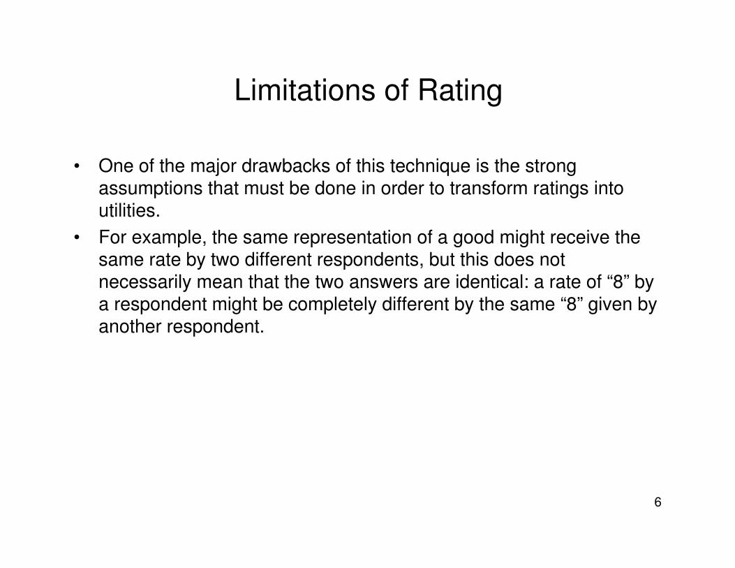
Limitations of Rating

• One of the major drawbacks of this technique is the strong assumptions that must be done in order to transform ratings intoutilities.

• For example, the same representation of a good might receive thesame rate by two different respondents, but this does not necessarily mean that the two answers are identical: a rate of “8” by a respondent might be completely different by the same “8” given by another respondent.

7

Conjoint Analysis

Would you prefer not to buy any of these cars?

Volkswagen Polo?

Ford Focus?

Fiat Punto?

Which would you buy?

1.184 dm31.205 dm31.080 dm3Baggage car

6.46.86Consumption (liters/100 km)

353Number of doors

171 km/h185 km/h172 km/hMaximum speed

AutomaticManualManualGear

139015961242Cubic capacity

555Number of Seats

£ 12,935£ 10,120£ 9,750Price

Volkswagen Polo

1.4 16V

Ford Focus

1.6 16V

Fiat Punto

1.2 16V ELXCars attributes

Suppose you are facing the choice of buying a new car. Choose one of the following cars according to your

preferences. You may even choose not to buy any of these cars.

8

Conjoint Analysis(conjoint choice analysis,

choice experiments, conjoint choice experiments)

• In a conjoint choice exercise, respondents are shown a set of alternative representations of a good and are asked to pick their most preferred.

• Similar to real market situations, where consumers face two or more goods characterized by similar attributes, but different levels of these attributes, and are asked to choose whether to buy one of the goods or none of them.

• Alternatives are described by attributes—the alternatives shown to the respondent differ in the levels taken by two or more of the attributes.

• The choice tasks do not require as much effort by the respondent as in rating or ranking alternatives.

9

• If we want to use conjoint analysis techniques for valuation purposes, one of the attributes must be the “price” of the alternative or the cost of a public program to the respondent.

• If the “do nothing” (or “status quo” option—i.e., pay nothing and get nothing) is included in the choice set, the experiments can be used to compute the value (WTP) of each alternative.

• Note that we only learn which alternative is the most preferred, but we do not know anything about the preferences for the options that have not been chosen the exercise does not offer a complete preference ordering.

10

Assuming that the following areas were the ONLY areas available, which one would you

choose on your next hunting trip, if either?

Features of the

hunting area Site A Site B

Distance from home to hunting area

50 km 50 km

Quality of road from home to hunting area

Mostly graved or dirt, some paved

Mostly paved, some gravel or dirt

Access within hunting area

Newer trails, cutlines or seismic lines,

passable with a 2WD vehicle

Newer trails, cutlines or seismic lines,

passable with a 4WD vehicle

Encounters with other hunters

No hunters, other than those in my hunting

party, are encountered

Other hunters, on ATVs, are encountered

Forestry activity Some evidence of

recent logging found in the area

No evidence of logging

Moose population Evidence of less than 1

moose per day Evidence of less than 1

moose per day

Neither Site A or Site B

I will NOT go moose hunting

Check ONE and only one box

Example of conjoint choice question from Boxall et al. (1996).

11

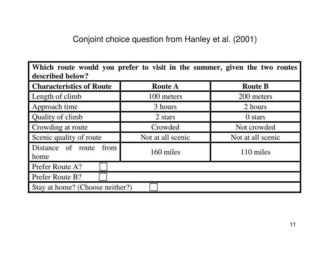
Conjoint choice question from Hanley et al. (2001)

Which route would you prefer to visit in the summer, given the two routes

described below?

Characteristics of Route Route A Route B

Length of climb 100 meters 200 meters

Approach time 3 hours 2 hours

Quality of climb 2 stars 0 stars

Crowding at route Crowded Not crowded

Scenic quality of route Not at all scenic Not at all scenic

Distance of route from home

160 miles 110 miles

Prefer Route A?

Prefer Route B?

Stay at home? (Choose neither?)

12

Example of conjoint choice question from San Miguel et al. (2000).

Which surgical procedure would you prefer in the treatment of menorrhagia?

Characteristics of the treatment Hysterectomy Conservative

Number of nights in hospital after operation 7 0

Time to return to normal activity (weeks) 11 2

Chance of complications following operation 45% 20%

Chance of re-treatment with Conservative 0% 15%

Chance of re-treatment with Hysterectomy 0% 30%

Cost of the treatment $1,400 $5,000

Which treatment would you prefer? (tick one box only) Prefer

Hysterectomy Prefer

Conservative

13

Example of conjoint question from Alberini et al. 2005

1) Land use

2) Moorings

3) New Buildings

4) Fast connections with other parts of the city

5) New jobs created

6) Cost (regional tax for year 2004)

No connections Yes connections

350 new jobs 350 new jobs

No new moorings No new moorings

No new buildings Yes new buildings

14

Why is conjoint analysis useful?

• Useful in non-market valuation, because it places a value on goods that are not traded in regular marketplaces.

• It can also be used to value products, or improvements over existing products—popular technique in marketing research.

• Allows one to estimate WTP for a good that does not exist yet, or under conditions that do not exist yet—for example, a lake after water pollution has been reduced, but people have always seen the lake as a polluted body of water.

• Allows one to elicit preferences and WTP for many different variants of goods or public programs, and so it can help make decisions about environmental programs where the scope of the program has not been decided upon yet (e.g., EPA’s arsenic in groundwater rule—should it be 50 ppb, 25 ppb, 10ppb?)

• An advantage of conjoint choice is that researchers usually obtain multiple observations per interview, one for each choice task from each respondent. This increases the total sample size for statistical modeling purposes, holding the number of respondents the same.

15

Designing a Conjoint Analysis Study

• 1st task: select the attributes that define the good to be valued. The attributes should be selected on the basis of what the goal of the valuation exercise is, prior beliefs of the researcher, and evidence from focus groups.

• For valuation, one of the attributes must be the “price” of the commodity or the cost to the respondent of the program delivering a change in the provision of a public good.

• Attributes can be quantitative, and expressed on a continuous scale, such as the gas mileage of a car, or the square footage of a house. The price or cost attribute should be on a continuous scale. Attributes can be of a qualitative nature, such as the style of a house (e.g., Cape Cod, ranch, colonial) or the presence/absence of a specified feature.

• It is also important to make sure that the provision mechanism, whether private or public, is acceptable to the respondent, and that the payment vehicle is realistic and compatible with the commodity to be valued.

16

• 2nd step: choose the levels of the attributes.• the levels of the attributes should be selected so as to be

reasonable and realistic, or else the respondent may reject the scenario and/or the choice exercise.

17

Attributes and levels used in the moose hunting study from Boxall et al. (1996).

Attributes Levels

Evidence of < 1 moose per day

Evidence of 1-2 moose per day

Evidence of 3-4 moose per day Moose population

Evidence of more than 4 moose per day

Encounters with no other hunters

Encounters with other hunter on foot

Encounters with other hunter on ATVa Hunter congestion

Encounters with other hunter in trucks

No trails, cutlines, or seismic lines

Old trails passable with ATVa

Newer trails, passable with 4-wheel drive vehicle Hunter access

Newer trails, passable with 2-wheel drive vehicle

Evidence of recent forestry activity Forestry activity

No evidence of forestry activity

Mostly paved, some gravel or dirt Road quality

Mostly gravel or dirt, some paved sections

50 km

150 km

250 km Distance to site

350 km aAll-terrain vehicles

18

Attributes and levels from San Miguel et al. (2000).

Attributes Levels

Nights in hospital after intervention 0, 2, 4 and 7*

Time to return to normal activity 2, 3, 4 and 11*

Chance of complications following the operation

5%, 10%, 15%, 20% and 45%*

Probability of re-treatment with conservative surgery

0%*, 10%, 20% and 30%

Probability of re-treatment with hysterectomy

0%*, 10%, 20% and 30%

Cost £500, £1200, £1400*, £2500 and £5000

*Levels defined for the fixed scenario of hysterectomy

19

Attributes and levels from Alberini et al. (2005).

1501005025Cost to the respondent

in Euro (4 levels)

350250150Number of new jobs

created (3 levels)

Not availableAvailable

Access (fast

transportation links

with

other areas of Venice,

the airport, the

mainland, other

islands) (2 levels)

Presence of new

buildings on the

25% of the

allowable area

No new buildings

New buildings in the

Northeast portion of

the Arsenale (2 levels)

200 new mooringsNo new mooringsUse of the water areas

(2 levels)

Shipbuilding,

research, museum

Hotels,

museum,

research

Housing, research,

museum

Shipbuilding,

research, offices,

museum

Land use

(4 levels)

Level 4Level 3Level 2Level 1Attribute

20

• 3rd task: be mindful of the sample size when choosing attributes and levels.

• Total sample size is given by the number of respondents × the number of conjoint choice questions in the questionnaire.

• The sample size should be large enough to accommodate all of thepossible combinations of attributes and levels of the attributes, i.e., the full factorial design.

• To illustrate, consider a house described by three attributes: • square footage, • proximity to the city center, and • price. • If the square footage can take three different levels (1500, 2000,

2200), proximity to the city center can take two different levels (less than three miles, more than three miles) and price can take 4 different levels (£200,000, £250,000, £300,000, and £350,000), the full factorial design consists of 3×2×4=24 alternatives. Fractionaldesigns are available that result in fewer combinations.

21

• 4th task: Once the experimental design is created, the researcher needs to construct the choice sets. The choice sets may consist of two or more alternatives, depending on how simple one wishes to keep the choice tasks.

• The “status quo” should be included in the choice set if one wishes to estimate WTP for a policy package or a scenario.

• This can be done in a number of different ways. For instance, one can ask the respondent to choose between A and the status quo, then B and the status quo, etc. Alternatively, one can ask the respondent to choose directly between A, B, and the status quo. Or, respondents may first be asked to indicate their preferred option between A and B (the so-called “forced choice”), and then they may be asked which they prefer, A, B or the status quo.

• When grouping alternatives together to form the choice sets, it is important to exclude alternatives that are dominated by others. For example, if house A and B were compared, and the levels of all attributes were identical, but B were more expensive, A would be a dominating choice.

• Such pairs should not be proposed to the respondents in the questionnaire, although some researchers believe that this is a way of checking if respondents are paying attention to the attributes of the alternatives they are shown.

22

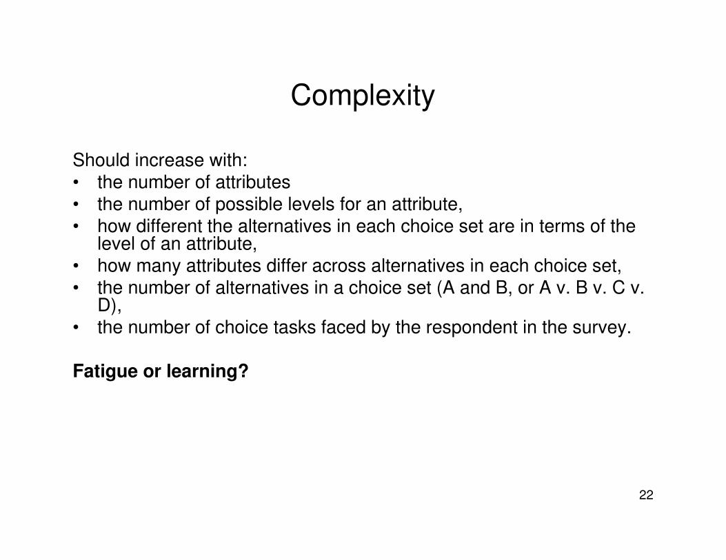
Complexity

Should increase with:• the number of attributes • the number of possible levels for an attribute, • how different the alternatives in each choice set are in terms of the

level of an attribute, • how many attributes differ across alternatives in each choice set, • the number of alternatives in a choice set (A and B, or A v. B v. C v.

D),• the number of choice tasks faced by the respondent in the survey.

Fatigue or learning?

23

Model for the Conjoint Analysis

It is assumed that the choice between the alternatives is driven by the respondent’s underlying utility. The respondent’s indirect utility is broken down into two components. The first component is deterministic, and is a function of the attributes of alternatives, characteristics of the individuals, and a set of unknown parameters, while the second component is an error term. Formally,

1)

where the subscript i denotes the respondent, the subscript j denotes the alternative, x is the vector of attributes that vary across alternatives (or across alternatives and individuals), and ε is an error term that captures individual- and alternative-specific factors that influence utility, but are not observable to the researcher. Equation (1) describes the random utility model (RUM).

ijijij VV ε+= ),( βx

24

We can further assume that the deterministic component of utility is a linear function of the attributes of the alternatives and of the respondent’s residual income, (y - C):

2)

where y is income and C is the price of the commodity or the cost of the program to the respondent.

The coefficient is the marginal utility of income.

Respondents are assumed to choose the alternative in the choice set that results in the highest utility. Because the observed outcome of each choice task is the selection of one out of K alternatives, the appropriate econometric model is a discrete choice model expressing the probability that alternative k is chosen. Formally,

3)

where signifies the probability that option k is chosen by individual i.

2β

ijjiijij CyV εββ +−++= 210 )(βx

kjVVVVVVV(V ijikiKikiikiikik ≠∀>=>>>= )Pr(),...,,Pr 21π

ikπ

25

This is very important!!!

This means that

4)

from which follows that

5)

Equation (5) shows the probability of selecting an alternative no longer contains terms in (2) that are constant across alternatives, such as the intercept and income.

It also shows that the probability of selecting k depends on the differences in the levels of the attributes across alternatives, and that the negative of the marginal utility of income is the coefficient on the difference in cost or price across alternatives.

kjCyCy ijijiijikikiikik ≠∀+−++>+−++= ))()(Pr( 210210 εββεββπ βxβx

kjCC ijikijikikijik ≠∀−−−<−= ))()()Pr[( 21 βεεπ βxx

kjCyCy ikijijiijikiikik ≠∀−>+−−−−++= )Pr( 22102210 εεββββββπ βxβx

26

Dataset in LIMDEP

Respon i picked nij taxes castello taca

1 1 0 3 25 0 0

1 2 0 3 50 0 0

1 3 1 3 0 0 0

1 4 0 3 100 0 0

1 5 0 3 25 0 0

1 6 1 3 0 0 0

1 7 0 3 50 0 0

1 8 0 3 100 0 0

1 9 1 3 0 0 0

1 10 0 3 50 0 0

1 11 0 3 150 0 0

1 12 1 3 0 0 0

2 1 1 3 100 1 100

2 2 0 3 150 1 150

2 3 0 3 0 1 0

2 4 0 3 150 1 150

2 5 1 3 50 1 50

2 6 0 3 0 1 0

2 7 0 3 100 1 100

2 8 0 3 150 1 150

2 9 1 3 0 1 0

2 10 1 3 150 1 150

2 11 0 3 100 1 100

2 12 0 3 0 1 0

12 obs per

respondent because

each respondent

answers 4 choice

questions and each

choice question has

3 alternatives (A,B

and status quo)

Left alternative Right alternative Status quo

Status quo is chosen

Right alternative

is chosen

Taxes*castello

Castello = dummy =1 if respondent lives in castello

nij=3 because in each choice task there are 3 options

From Alberini et al

2005

27

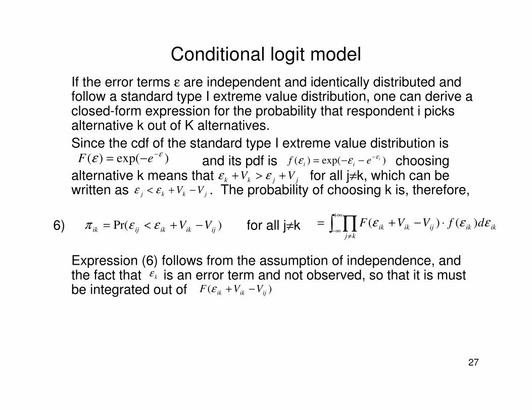
Conditional logit model

If the error terms ε are independent and identically distributed and follow a standard type I extreme value distribution, one can derive a closed-form expression for the probability that respondent i picks alternative k out of K alternatives.

Since the cdf of the standard type I extreme value distribution is

and its pdf is choosing alternative k means that for all j≠k, which can be written as . The probability of choosing k is, therefore,

6) for all j≠k

Expression (6) follows from the assumption of independence, and the fact that is an error term and not observed, so that it is must be integrated out of

)exp()( εε −−= eF )exp()( ief ii

εεε −−−=

jjkk VV +>+ εε

jkkj VV −+< εε

)Pr( ijikikijik VV −+<= εεπ ikik

kj

ijikik dfVVF εεε )()( ⋅−+= ∫ ∏+∞

∞−≠

kε

)( ijikik VVF −+ε

28

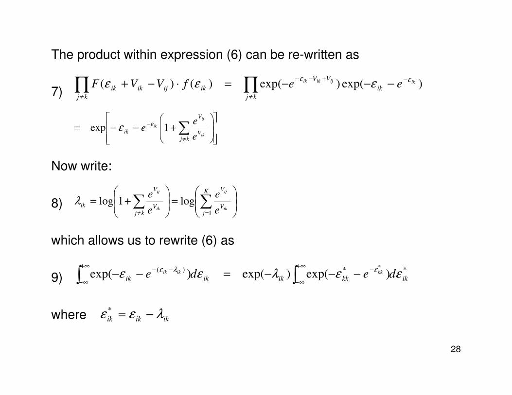
The product within expression (6) can be re-written as

7)

Now write:

8)

which allows us to rewrite (6) as

9)

where

∏∏≠

−+−−

≠

−−−=⋅−+kj

ik

VV

ik

kj

ijikikikijikik eefVVF )exp()exp()()( εε

εεε

+−−= ∑

≠

−

kjV

V

ikik

ij

ik

e

ee 1exp εε

=

+= ∑∑

=≠

K

jV

V

kjV

V

ikik

ij

ik

ij

e

e

e

e

1

log1logλ

**)( )exp()exp()exp(*

ikkkikikik dede kkikik εελεε ελε

∫∫+∞

∞−

−+∞

∞−

−− −−−=−−

ikikik λεε −=*

29

The integrand in expression (9) is the pdf of the extreme value distribution and is, clearly, equal to 1. Equation (9) thus simplifies to

which by (8) is in turn equal to

Recalling (2), the probability that respondent i picks alternative k out of K alternatives is

10)

where is the vector of all attributes of alternative j, including cost,

and =

)exp( ikλ− ∑=

K

j

ijik VV1

)exp(/)exp(

∑=

=K

j

ij

ik

ik

1

)exp(

)exp(

βw

βwπ

=

ij

ij

ij C

xw

β

− 2

1

β

β

30

Equation (10) is the contribution to the likelihood in a conditional logit model. The full log likelihood function of the conditional logitmodel is

11)

where yik is a binary indicator that takes on a value of 1 if the respondent selects alternative k, and 0 otherwise. The coefficients are estimated using the method of Maximum Likelihood (MLE).

∑∑= =

⋅=n

i

K

k

ikikyL1 1

loglog π

31

We can further examine the expression for in equation (10) to show that depends on the differences in the level of the attributes between alternatives. To see that this is the case, we begin by re-writing (10) as

12)

which is equal to

13)

and thus to

14)

ikπ

ikπ

++++==

∑=

)exp()exp()exp(

)exp(

)exp(

)exp(

1

1

βwβwβw

βw

βw

βw

iKiki

ik

K

j

ij

ikik

KKπ

1

1

)exp(

)exp()exp()exp(−

++++=

βw

βwβwβw

ik

iKiki KK

[ ] [ ] 1

1 )(exp1)(exp−

−++++−= βwwβww iKikiki KK

32

For large samples and assuming that the model is correctly specified, the maximum likelihood estimates are normally

distributed around the true vector of parameters ββββ, and the asymptotic variance-covariance matrix, Ω, is the inverse of the Fisher information matrix. The information matrix is defined as

15)

where

β

)()()(1 1

′−−=∑∑= =

iik

n

i

K

k

iikikI wwwwπβ

∑=

=K

k

ikiki

1

ww π

33

Marginal Prices and WTPOnce model (11) is estimated, the rate of trade off between any two

attributes is the ratio of their respective β coefficients. The marginal value of attribute l is computed as the negative of the coefficient on that attribute, divided by the coefficient on the price or cost variable:

16)

The willingness to pay for a commodity is computed as:

17)

where x is the vector of attributes describing the commodity assigned to individual i. It should be kept in mind that a proper WTP can only be computed if the choice set for at least some of the choice sets faced by the individuals contains the “status quo” (in which no commodity is acquired, and the cost is zero). Expression (17) is obtained by equating the indirect utility associated with commodity and residual income

with the indirect utility associated to the status quo (no commodity) and the original level of income y, and solving for C.

2ˆ

ˆ

β

β llMP −=

2

1

ˆ

ˆ

β

βx i

iWTP −=

ix)( Cy −

34

Is conjoint analysis better than contingent valuation?

• Several analysts believe that conjoint analysis questions reducestrategic incentives, because individuals are busy trading off the attributes of the alternatives and are less prone to strategic thinking (Adamowicz et al., 1998).

• The same reasoning and the fact that conjoint choice questions may appear less “stark” than the take-it-or-leave options of contingent valuation has led other researchers to believe that “protest”behaviors are less likely to occur in conjoint analysis surveys.

• Some valuation researchers (Carson, Hanemann) do not believe in conjoint analysis because they believe that much effort must be spent in stated preference studies to provide a scenario that is fully understood and accepted by the respondent. Changing this scenario from one choice question to the next, they point out, results in a loss of credibility of the scenario and may induce rejection of the choice task.

35

Descriptive statistics from Alberini et al. 2005 Table 2. Individual Characteristics of the Respondents (categorical variables).

Percentage of the sample who:

Is a resident of the city of Venice 88.10

Has visited the Arsenale 72.35

Is a male 52.43

Is married 9.32

Is gainfully employed 25.40

Is currently looking for a job 14.79

Is a student 42.44

Is a homemaker 0.32

Is a retiree 3.86

Has a college degree 47.27

Owns a boat 19.61

Has gone to the theater at least once in the last 12 months 72.03

Belongs to an Environmental Organization 36.01

Belongs to a Civic Association 12.22

Has visited a museum or art exhibit over the last 12 months 91.64

Table 3. Individual Characteristics of the Respondents (continuous variables).

mean Std. deviation minimum Maximum

Age 31.90 11.32 17 78

Household income 29741.10 24600.99 7500 100000

Years of schooling 16.01 3.07 5 21

Household size 3.35 2.09 1 26

36

Table 10. Conditional logit model of the responses to the choice questions. Obs 892.

Specification A Specification B Specification C Specification D

coeff t -stat Coeff t -stat coeff t -stat coeff t -stat

STATUSQUO -1.5838 -13.7415 -1.0411 -3.7415

MOORINGS 0.2182 1.9270 0.2438 2.0807 0.2259 1.8985

NEW_CONS -0.1175 -1.0741 0.2808 2.1674 0.2646 2.0237

CONNECTI 0.7095 6.9944 0.7673 7.1876 0.6311 4.9854

JOBS 0.0018 2.3532 0.0045 3.7096 0.0045 3.6275

TAXES -0.0039 -2.7647 -0.0059 -3.7346 -0.0060 -3.7496

LANDUSE1 0.2725 0.7474 0.3034 0.8247

LANDUSE2 0.7762 2.6638 0.3495 1.0870

LANDUSE3 -0.9163 -2.2960 -0.6451 -1.5760

LANDUSE4 0.4768 1.2407 0.5315 1.3708

LANDUSE3 * (DUMMY TOURISTS)1

-0.7404 -2.3349

LANDUSE2 * (DUMMY ABITARE)2

1.1860 3.9800

CONNECTI * (DUMMY LINKS)3

0.3948 1.9814

0.2259 1.8985

log likelihood -836.8628 -804.442 -755.4047 -742.0907 1 DUMMY TOURISTS = dummy variable that takes on a value of 1 if a respondent rates the presence of tourists as 4 or 5 on a scale where 1 means not important at all and 5 very important. 2 DUMMY ABITARE = dummy variable that takes on a value of 1 if a respondent rates the cost of housing as 4 or 5 on a scale where 1 means not important at all and 5 very important. 3 DUMMY LINKS = dummy variable that takes on a value of 1 if a respondent rates the presence of fast transportation connections as a prerequisite for the optimal reuse of the Arsenale as 5 on a scale where 1 means not important at all and 5 very important.

Results from Alberini et al. (2005).