choosing to grow a graph: modeling network formation as
TRANSCRIPT

Choosing to Grow a Graph:Modeling Network Formation as Discrete ChoiceJan Overgoor
Stanford UniversityStanford, CA
Austin R. BensonCornell University
Ithaca, [email protected]
Johan UganderStanford University
Stanford, [email protected]
ABSTRACTWe provide a framework for modeling social network formationthrough conditional multinomial logit models from discrete choiceand random utility theory, in which each new edge is viewed asa “choice” made by a node to connect to another node, based on(generic) features of the other nodes available to make a connec-tion. This perspective on network formation unifies existing modelssuch as preferential attachment, triadic closure, and node fitness,which are all special cases, and thereby provides a flexible meansfor conceptualizing, estimating, and comparing models. The lens ofdiscrete choice theory also provides several new tools for analyzingsocial network formation; for example, the significance of nodefeatures can be evaluated in a statistically rigorous manner, andmixtures of existing models can be estimated by adapting knownexpectation-maximization algorithms. We demonstrate the flexi-bility of our framework through examples that analyze a numberof synthetic and real-world datasets. For example, we provide rig-orous methods for estimating preferential attachment models andshow how to separate the effects of preferential attachment and tri-adic closure. Non-parametric estimates of the importance of degreeshow a highly linear trend, and we expose the importance of look-ing carefully at nodes with degree zero. Examining the formationof a large citation graph, we find evidence for an increased role ofdegree when accounting for age.
KEYWORDSSocial networks; network formation; choice models
ACM Reference Format:Jan Overgoor, Austin R. Benson, and Johan Ugander. 2019. Choosing to Growa Graph: Modeling Network Formation as Discrete Choice. In Proceedingsof the 2019 World Wide Web Conference (WWW ’19), May 13–17, 2019, SanFrancisco, CA, USA. ACM, New York, NY, USA, 12 pages. https://doi.org/10.1145/3308558.3313662
1 INTRODUCTIONUnderstanding how networks form and evolve is an essential com-ponent of understanding their structure, which in turn underliesthe basis for understanding the broad range of processes that oc-cur on networks. Models of social network formation can largelybe decomposed into node formation and edge formation. In this
This paper is published under the Creative Commons Attribution 4.0 International(CC-BY 4.0) license. Authors reserve their rights to disseminate the work on theirpersonal and corporate Web sites with the appropriate attribution.WWW ’19, May 13–17, 2019, San Francisco, CA, USA© 2019 IW3C2 (International World Wide Web Conference Committee), publishedunder Creative Commons CC-BY 4.0 License.ACM ISBN 978-1-4503-6674-8/19/05.https://doi.org/10.1145/3308558.3313662
work, we argue that edge formation can be effectively modeled asa choice made by an actor (or actors) in the network to instantiatea connection to another node. The diverse research on networkformation has led to many models and mechanisms of edge for-mation, including preferential attachment [2], uniform attachment[12], triadic closure [31], random walks [65, 78], homophily [55],copying edges from existing nodes [35, 39], latent space structures[22, 41, 55], inherent node fitness [7, 11], and combinations of all ofthese [28, 40, 43]. Here, we frame edge formation as a discrete choiceprocess and derive a family of discrete choice models [47, 74] thatsubsume a wide range of existing models in a unified frameworkand also naturally opens up a host of powerful extensions.
Discrete choice models are commonly employed in economics,social psychology, and statistics as a way to model how individualsmake choices from a slate of discrete alternatives [1]. Typically,the alternatives have associated features, and statistical models ofdiscrete choice make it possible to estimate the relative importanceof such features. Such models have been used to answer questionssuch as how consumers choose goods [67], how people choosewhere they live [46], how students choose what college to attend[21], and how commuters choose between different modes of trans-portation [75]. Discrete choice analysis is also used to understandhow choices vary depending on the context in which they areframed: in online commerce, this could be how web layouts leadto different purchasing priorities [26]; for choosing colleges, thiscould be incorporating the effect of the national economy. In thispaper, we demonstrate how discrete choice models can similarlyhelp us understand the factors driving social network evolution.
The starting point for the present work is the observation thatedge formation events in social networks are naturally viewed asdiscrete choices. For simplicity, consider a directed graph whereedges are formed one by one, where we can think of the formationof a directed edge (i, j ) as i “choosing” to connect with j , where theset of alternatives available to i is the set of all other nodes. (Whileundirected graph models are common in social network analysis,the underlying formation procedure is almost always asymmetric.For example, the Facebook friendship graph is typically modeled asan undirected graph [77], but the friendships are proposed by oneof the two nodes in an edge.) The key modeling question is easy tostate: why did i choose j? This question has long been the informalsubject of network formation modeling and at the same time theexact question that discrete choice models and analysis have beendesigned to answer. However, up to this point, network formationmodels have largely been decoupled from discrete choice theory.
In employing discrete choice analysis, we focus on the condi-tional multinomial logit model, commonly called the conditionallogit model for short, which is a foundational workhorse of discrete
1409

choice modeling. The model belongs to the family of random utilitymodels, where choices are interpretable as those of a rational actorselecting the alternative with the largest “utility” sampled fromrandom variables that decompose into the inherent utility of thealternative and a noise term. With the conditional logit model, wecan use existing optimization routines to estimate model parame-ters and existing statistical methods to asses the uncertainty of theestimates. Discrete choice models can also easily restrict the set ofavailable alternatives, where it might not be reasonable to assumethat the entire set of nodes is available for friendship. For example,sometimes only “friends of friends” are considered [24, 28, 40].
In this paper, we first show thatmany popular network formationmechanisms can be rewritten as conditional logit models, includingpreferential attachment, uniform attachment, node fitness, latentspace models, and models of homophily. However, the real powerof discrete choice models for social network analysis is the abilityto combine different features (e.g., node degree and node age), aswell as different mechanisms (e.g., triadic closure and preferentialattachment) and estimate their relative roles. Social networks areenormously varied in their structure [27], but existing methodsoften do a poor job at modeling this diversity. Thus, beyond unify-ing the network formation and discrete choice literature, we alsodevelop several new tools for social network analysis. For example,we show how to estimate models to distinguish the effects of pref-erential attachment and triadic closure. We demonstrate these toolsby analyzing the formation of the Flickr social network and theformation of a citation network. We find on Flickr that accountingfor triadic closure greatly reduces the estimated role of degree inchoosing who to connect to, and that nodes with degree zero have aremarkably high utility. Our estimates of preferential attachment inthe citation network are similar to those observed in prior studies.When accounting for the age of a paper, we find evidence for linearpreferential attachment. However, for a fixed degree, we find thatage is negatively correlated with the likelihood of a new citation(i.e., older papers are less likely to be cited).
The key assumption underlying our framework is that the avail-able data actually captures edge formation events (either throughedge timestamps or other sequential information). In contrast, manyexisting approaches to understanding network formation focus onobserving only the structural properties of a network at a singlepoint of observation, e.g., its degree distribution, and initiating adeductive process to try and understand how variations in edgeformation would lead to different outcomes [2, 7, 28, 43]. This ap-proach leads to tidy analyses and easy-to-characterize asymptoticproperties, but model selection in this context is strongly dependenton what properties are compared. Different underlying formationprocesses can lead to graphs with indistinguishable properties. Forexample, many different formation processes result in the sameheavy-tailed degree distributions [52]. Thus, when “fitting” out-come measurements in this way, one has to know (or posit), e.g.,the relative rates of node formation and edge formation. However,when temporal or sequential data is available [25, 56], our frame-work overcomes these limitations by incorporating this structure.Additional related work. There is a strong connection betweenour work and work on link prediction and missing data methods us-ing network features to predict edges [15, 42]. A network formation
model implicitly makes claims about what edges are most likely toform next, and thus can be evaluated by the same metrics as linkprediction algorithms [44]. We use predictive accuracy as a measureof goodness of fit, but our primary concern is interpretability ofthe model and estimates, which is one of the advantages of theconditional logit model.
In sociology, stochastic actor-oriented models (SAOMs) employa similar logit choice [69, 70]; however, these models are targetedtowards data collected as a few snapshots rather than edge-by-edgeformation. SAOMs also model the rate at which nodes form newrelationships, whereas we condition on the node initiating the newedge, providing better estimates of model parameters. There arealso sociological models such as relational event models [10] anddynamic network actor models [71] that use fine-grained temporalinformation, yet these also do not condition on the initiator node aswe do. While these sociological models can incorporate notions ofnetwork formation (e.g., preferential attachment), our conditionallogit framework actually cleanly subsumes a wide range of modelsas special cases.
Finally, estimating the parameters that drive edge formation isdifferent from identifying the factors that could have lead to theobserved graph. The latter question is often pursued with so-calledexponential random graph models (ERGMs) [63, 79, 81]. However,these models do not consider individual edge events, are hard toestimate, and have known pathologies [13, 66].
2 DISCRETE CHOICE AND EDGEFORMATION
We now develop network formation through the lens of discretechoice. Throughout this paper, we assume that the networks aredirected. Again, while undirected graphs are common in social net-work analysis, the actual edge formation process often has directedinitiation. In the common setting of “growing graphs,” nodes arriveone at a time and form edges when arriving in a network. In thesecases, the newly arriving node is considered to be the node initi-ating the connection; such analysis is standard with, e.g., classicalpreferential attachment models [2].
When modeling the directed formation of an edge (i, j ), twoprocesses need to be distinguished, roughly corresponding to thequestions “who is i?” (the chooser) and “who is j?” (the chosen). Inthis paper, we focus on understanding the latter, i.e., the formationof (i, j ) as the selection of j conditional on knowing that i is ready toform an edge. Thus, our discrete choice models of edge formationcan be readily estimated from data that implicitly or explicitlycontains a record of initiating i nodes and used for subsequentanalysis, as we show in Sections 3 and 4. Beyond the scope of thiswork, our model of “j conditional on i” can be paired with a model of“initiations by i” for a full generative model of network formation.
2.1 Background on discrete choice modelsWe now review discrete choice models generically, which we willthen translate to the context of edge formation in Section 2.2. Con-sider a universe of alternatives X and a dataset consisting of ndifferent choices, indexed by k = 1, . . . ,n. Each choice (j,C ) con-sists of a choice set C ⊆ X and a chosen item j ∈ C . The elementsin C are mutually exclusive choice alternatives, and exactly one
1410
element from C is chosen. We consider each element j ∈ C to berepresented by a vector of features x j (for example, in our analysisin Section 2.2, x j will be the feature vector of a node in the graph,and C will represent a set of nodes). We let D = {(jk ,Ck )}nk=1denote the choice data.
A broad family of discrete choice models is the family of randomutility models (RUMs), of which the conditional logit is an importantspecial case. Each alternative j has some inherent utility to the agenti making the choice; with the conditional logit, we model this utilityas a linear function of j’s features x j :
ui, j = θT x j ,
for some (latent) parameter vector θ that is fixed across individuals i .Random utility models assume that agents make “rational” choicesby maximizing random utilities centered on these inherent utilities.More formally, the utility Ui, j observed by the actor is given byUi, j = ui, j + εi, j , where εi, j is a noise term. The probability Pi (j,C )of i choosing option j from the choice set C is
Pi (j,C ) = Pr(j = argmaxℓ∈C
Ui, ℓ ).
When the εi, j are i.i.d. standard Gumbel, the probability of choos-ing each alternative is proportional to the exponentiated inherentutility [1]:
Pi (j,C ) =expθT x j∑
ℓ∈C expθT xℓ. (1)
The above model is the conditional multinomial logit model ofdiscrete choice, though it is often referred to simply as the condi-tional logit or multinomial logit (MNL) model. If the noise termsεi, j are distributed i.i.d. Normal, then the model is the independentmultinomial probit. In probit models, the choice probabilities areno longer proportional to utilities as in Equation (1). The Gumbelassumption is common in discrete choice theory and will facilitateour connections to a variety of network formation mechanisms.There are more complex random utility models that can imposedependence between noise terms [74] and there also is a growingliterature of flexible choice models [4, 60, 76] designed to modelcontext effects and other varied violations of the independence ofirrelevant alternatives [45] (a storied axiom satisfied by the condi-tional multinomial logit model). We leave the relationships of thesemodels to network formation as avenues for future research.
2.2 Edge formation as discrete choiceWith the above formalisms in place, we now develop network for-mation from a discrete choice perspective. We begin by showinghow several well-known models can be conveniently expressed asconditional logit models, with a summary given in Table 1. All mod-els are designed to grow simple graphs (i.e., without multi-edges),and the choice set C excludes any nodes to which the chooser i isalready connected. Every item is represented by its features that,importantly, can evolve over time. The features x j,t of node j attime t are thus always time-indexed, but we often suppress the t toreduce notational clutter.Preferential attachment. We start with the generalized Barabási-Albertmodel [2, 8, 36], also known as the generalized Pricemodel [59],one of the most studied models in the network formation literature.
It is typically stated as a growth model of a time-evolving graphGt = (Vt ,Et ), t = 1, 2, 3, . . ., and when a new node arrives it con-nects tom distinct existing nodes j with a probability proportionalto a power of their degree dj,t at time t ,
P (j,Vt ) =dαj,t∑
ℓ∈Vt dαℓ,t. (2)
The exponent parameter α controls the relative importance of de-gree [36]. The case where α = 1 is called linear preferential at-tachment, and produces networks that can mimic a range of struc-tural properties observed in empirical networks. If we representeach potential neighbor j with the time-indexed one-dimensional“feature vector” x j,t = logdj,t and employ a conditional logitmodel as in Equation (1), we obtain a utility of j for i at time tof ui, j,t = θ logdj,t . Here the choice model parameter θ plays theexact role of α , since eθ logdj,t = dθj,t .
Given a growing network Gt , we can construct a choice datasetD from this network by extracting the node jt , node sets Vt , anddegree sequence (d1,t , . . . ,d |Vt |,t ) at each time-step. The prefer-ential attachment model has only one parameter, θ = α . The log-likelihood for that parameter given a dataset is then:
l (α ;D) =∑
(j,C )∈D
logexp(α logdj )∑
ℓ∈C exp(α logdℓ )
=∑
(j,C )∈D
*,α logdj − log
∑ℓ∈C
exp(α logdℓ )+-.
We’ve suppressed the time-index t from the features logdℓ to reduceclutter, but emphasize that dℓ is the degree at the time of the choice.Non-parametric preferential attachment. The above model as-sumes an attachment kernel of a particular parametric form. From adiscrete choice perspective, one can also estimate the role of degreein edge formation non-parametrically by estimating a coefficient θkfor each degree k = 0, . . . ,n − 1 individually. This approach has theadded benefit of being able to assign positive probability to choos-ing nodes with degree zero. Under this model, the log-likelihood ofthe parameters θ = (θ0, ...,θn−1) given the dataset is:
l (θ ;D) =∑
(j,C )∈D
logexpθdj∑
ℓ∈C expθdℓ
=∑
(j,C )∈D
*,θdj − log
∑ℓ∈C
expθdℓ +-.
Again we’ve suppressed time-indexing to simplify the presenta-tion. Pham et al. [58] previously described a version of the abovelikelihood as a means of measuring the attachment kernel usingmaximum likelihood, albeit without making the connection to dis-crete choice.Uniform attachment. A simple edge formation model is to sam-ple a new neighbor uniformly at random from all nodes [12]. Thereare no parameters in this model, but we can still write down thelikelihood of the model given a dataset, which will be useful whenwe later combine this model with others within a mixture model:
l (D) =∑
(j,C )∈D
logexp (1)∑
ℓ∈C exp (1)=∑
(j,C )∈D
− log |C |.
1411

Table 1: Network formation models framed as utility func-tions for a conditional logit. Where appropriate, we use thetraditional notation for the parameters of each process.
Process ui, j C
Uniform attachment [12] 1 VPreferential attachment [2, 36] α logdj VNon-parametric PA [54, 58, 62] θdj V
Triadic closure [61] 1 {j : FoFi, j }FoF attachment [31, 65, 78] α logηi, j VPA, FoFs only α logdj {j : FoFi, j }Individual node fitness [11] θ j VPA with fitness [6, 53] α logdj + θ j VLatent space [22, 41, 55] β · d (i, j ) VStochastic block model [33] ωдi ,дj VHomophily [48] h · 1{дi = дj } V
Triadic closure. A variant of uniform attachment is for i to attachto new neighbors uniformly at random from the set of their friends-of-friends, as opposed to the set of all nodes. This process effectivelymodels triadic closure [61]. It has the same simple functional form ofthe uniform model, but now the choice set C varies with each choice,namely, the choice set is restricted to be only the friends of friendsof node i (the chooser) to which i is not already connected. Thischange in choice set can also be achieved by assuming the utilityof j to i at time t is ui, j,t = log(1{FoFi, j,t }), where 1{FoFi, j,t } is aboolean indicating whether i and j are friends of friends at time t ,and then letting the choice set revert to the full node set.
An additional model that naturally combines the ideas of pref-erential attachment and befriending friends-of-friends takes thenumber of friends in common between i and j as a feature. Wecould define this feature as ηi, j,t = |{k : ei,k,t ∧ ek, j,t }|, whereei,k,t indicates whether there is an edge between i and k at timet . The corresponding utility would be ui, j,t = α logηi, j,t . Thismodel is similar (but not equivalent) to random walk-based forma-tion models [31, 65, 78], which emphasize formation within a localneighborhood.Node fitness. Another line of formation models that is subsumedby the discrete choice framework are those involving fitness. Inthis work, nodes choose to connect to others based on some intrin-sic latent fitness score. Certain distributions of fitness values leadto a scale-free degree distribution [11], providing an alternativeexplanation to preferential attachment for modeling such degreedistributions. We can express the node fitness model by a condi-tional logit model with separate fixed effect θ j for each node j (sothe feature of a node is an indicator vector of its identity). Thelikelihood of the fitness parameters θ given the data is then:
l (θ ;D) =∑
(j,C )∈D
logexpθ j∑
ℓ∈C expθℓ
=∑
(j,C )∈D
*,θ j − log
∑ℓ∈C
expθℓ+-.
This formation model is equivalent to the classic Bradley-Terry-Luce model of discrete choice for estimating the quality of alter-natives [45]. Alternatively, one could replace the individual fixed
effects with surrogate features of node fitness such as an auxiliarymeasure of gregariousness (in the case of social networks), or theimpact factor of a paper’s journal (in the case of citations networks).
A related model proposes selection probabilities proportional tothe product of node fitness and degree [6, 53]. This model can bewritten as a conditional logit model with ui, j,t = α logdj,t + θ j .Latent space models. Another class of network formation mod-els postulates the existence of a latent space that drives connec-tions between nodes. Examples of latent spaces include Euclideanspace [22], hyperbolic space [37], a tree [41], a circle [55], or a set ofdiscrete classes [23]. While the conditional logit model in the formthat we describe it does not facilitate finding the best-fitting latentspace assignment to explain the data, it can be used to estimatethe relative importance of a known latent space given a distancefunction d (i, j ). As one example from the family of latent spacemodels, in the community-guided attachment (CGA) model [41] allnodes have a distance derived from the height h(i, j ) of commonparents in a latent tree structure situating all nodes i and j. Giventhis tree as known, a node connects to another proportionally toc−h (i, j ) for some scalar c > 0. As a conditional logit model, the cor-responding utility function is ui, j = −h(i, j ) · log(c ). The parametervector θ = log c can be retrieved by fitting a conditional logit witha known h(i, j ) as the only variable and transforming the estimatedparameter with c = exp(θ ). Assuming that the latent space repre-sentation is given is a strong assumption, and fitting such a modelwhile estimating the latent space representation (e.g. as done byHoff et al. [22] in Euclidean space) is much more difficult.Additional models. Conditional logit models are very flexibleand can deal with multiple features and interactions between them.Any number of features can be added, including node covariatesand structural features like a node’s clustering coefficient [3] orage [12, 40]. Conditional logit models can also be used to investigatethe role of homophily [48] in edge formation, by adding a binaryfeature indicating whether nodes i and j are part of the same class.
Table 1 summarizes how several network formation models fitwithin the discrete choice framework via their corresponding utilityfunctions and choice sets. A major advantage of this framework isthat different features can easily be combined into a single modeland jointly estimated. Or, when suitable, one can employ a mixtureof conditional logit models, as we show in the next section.
2.3 Combining modes using Mixed LogitSo far we have written a range of existing and new edge formationmodels as conditional logit models, a specific type of discrete choicemodel. But several existing edge formation models that do not fitneatly into the conditional logit framework, meanwhile, align ex-actly with the use of mixture models in discrete choice modeling.Following our success formulating edge formation models as condi-tional logit models, in this subsection we develop mixed conditionallogit formulations of several additional models.
A common proposal to make network formation models moreflexible is to augment an existing model by allowing nodes to pickneighbors uniformly at random with some probability 1 − p, whilerunning the ordinary model with probability p [17, 35, 39, 43]. Thisaugmentation increases flexibility because it enables the modelto explain edge events that may otherwise have probability zero.
1412

Within discrete choice, this approach is precisely a mixed logitmodel where one of the mixture modes is uniform attachment.
While the conditional logit estimates a single parameter vectorrepresenting average preferences as shared by all agents, the mixedlogit model is often used to account for differences in preferencesacross various types of agents. In its most general form, the mixedlogit is expressed using a probability distribution f over differentinstantiations of the parameter vector θ :
Pi (j,C ) =
∫ expθT x j∑l ∈C expθT xl
f (θ ) dθ .
In this work, we will only consider discrete mixtures of M logits,also called a latent class model [32]:
Pi (j,C ) =M∑
m=1πm
expθTmx j∑l ∈C expθTmxl
,
where∑Mm=1 πm = 1 and the weights π1, . . . ,πM model the relative
prevalence of each mode.Copy model. The copy model is a classic formation process thatcan be written as a mixed logit with two modes. In the first mode,new edges connect proportional to degree with probability p, whilein the second mode they connect uniformly at random with prob-ability 1 − p [17, 43]. As a conditional logit model, the utilities ofthe two modes are u (1)x = logdx and u
(2)x = 1, respectively, and
the class probabilities are (π1,π2) = (p, 1 − p). (This is a specialcase of the original copy model where d edges are copied froma sampled vertex [39]; the model here is when d = 1, which isoften used for analysis [19].) The connection between relaxationsof preferential attachment and mixture models was also recentlyobserved by Medina et al. [49].Local search model. Another example of a model with multiplemodes is the Jackson-Rogers model of edge formation as a mixtureof uniform attachment and triadic closure [24, 28]. The originalmodel is based on a relative rate r∗ between edges forming atrandom and edges formed locally. It also has edges form based onrespective acceptance probabilities.We describe a simplified versionof this model, which we’ll call the local search model, where edgesconnect to nodes selected uniformly at random from the full nodeset with probability r and uniformly at random from the set offriends-of-friends with probability 1 − r .1 We can represent thissimplified process with a two-mode mixed logit model. In this casethe mixture parameters are (π1,π2) = (r , 1 − r ) and both modeshave the same utility function ux = 1 but their choice sets differ sothat the second mode only considers friends-of-friends.2
Table 2 overviews the mixture model formulations describedabove, as well as a new model—the (r ,p)-model—that we use inSection 4.2 to analyze preferential attachment effects.
3 ESTIMATION AND INFERENCETo learn a discrete choice model of network formation from data,we assume that we have access to a sequence of directed edges, in1 Since the r ∗ parameter in the original presentation is actually the rate of uniformattachment, we can relate it to our r through r = r ∗
1+r ∗ . For example, if the ratebetween random and friend-of-friend edges is one to one (r ∗ = 1), then r = 0.5.2A model with a restricted choice set, for example to only friends-of-friends, gives alikelihood of zero to choices outside the choice set.
Table 2: Network formation models framed as mixed logits.Each mixture component is a mode. FoF refers to friend-of-friending, also called local search or triadic closure. We de-fine a new (r ,p)-model as a natural generalization of priorideas once we put network formation models in the lan-guage of discrete choice.
Process Modes
Copy model [35] Uniform, PANode types [38] New node, PA, noneLocal search [24, 28] Uniform, Uniform FoF(r ,p)-model Uniform, PA, Uniform FoF, PA FoF
chronological order. This sequence of edges needs to be recast aschoice data in order to fit a choice model. For every formed edge(i, j ), we create a data point consisting of the choice j , the choice setof candidates nodes at the time, and the features of each candidatenode at the time.
Given a data set and a conditional logit model, one can writeout the log-likelihood, as shown in Section 2.2. For any conditionallogit model with a linear utility ui, j = θT x j , the likelihood functionis convex with respect to the variables θ and can be efficientlymaximized using standard gradient-based optimization (e.g., BFGS).The functional form of the logit leads to straightforward gradients.For example, for preferential attachment, the gradient is
∂
∂αl (α ;D) =
∑(x,C )∈D
*,logdx −
∑y∈C logdy · exp(α logdy )∑
y∈C exp(α logdy )+-,
where the time-dependence of the features (degrees) have beensuppressed to reduce clutter. Gradients for the other choice modelsin Section 2.2 are omitted but straightforward.
One advantage of likelihood-based model fitting is that we cancompute standard errors and confidence intervals of the parameters.In particular, the standard errors can be computed with
√H−1 [74],
where H is the Hessian matrix of second derivatives of the log-likelihood at the parameters.Mixture models and expectation-maximization. For mixedconditional logit models, the log-likelihood is no longer convex ingeneral, making optimization more difficult. To maximize the like-lihood of mixed models we turn to expectation maximization (EM)techniques [18, 73]. We briefly summarize the procedure describedin Train’s book [74, Chapter 14.3.2]. Assume that we have a modelwithM modes (i.e., mixture components), where every mode startswith initial parameter values θ⃗m (usually initiated at 1). Choices(xk ,Ck ) ∈ D are again indexed with k , so that k ∈ {1, . . . ,n} andn = |D|. The EM algorithm runs through the following steps:
(1) Initiate class probabilities uniformly with πm = 1/M andinitial class responsibilities γmk = 1/M for each data point.
(2) For every data point k and every modem, compute the classresponsibility given by the relative individual likelihood:
γmk =πm · L
m (θm ; (xk ,Ck ))∑Mℓ=1 πℓ · L
ℓ (θ ℓ ; (xk ,Ck )).
(3) For every modem, update the total class probability withπm =
1N∑Nk=1 γ
mk .
1413
(4) For every modem, update the parameters θ⃗m using standardoptimization for fitting a single model, weighing each choiceset with its class responsibility γmk .
(5) Repeat steps 2–4 until some convergence or stopping criteria.The total likelihood of the parameters and class probabilities is:
l (θ ;D) =M∑
m=1lm (θm ;πm ;D) =
M∑m=1
N∑k=1
logLm (θm ; (xk ,Ck ))·πm
We monitor the convergence of the iterative procedure using thechange in this total likelihood between iterations.
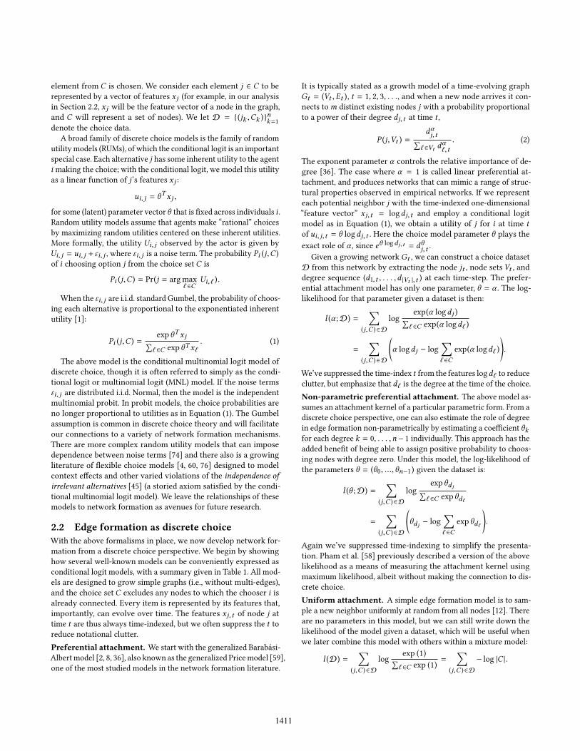
Even though EM is theoretically an efficient estimator [82], thereare cases when alternatives are appropriate. For example, if one hasreasonable bounds or priors on the parameter values, then directlikelihood maximization could be used, and if the search space islow-dimensional, a grid search might be appropriate. Recent theo-retical work has also developed algorithms for learning mixtures oftwo multinomial logit modes with theoretical guarantees assuminga separation between the modes [14].Negative sampling. Every time an edge is formed by some nodei , each node not yet connected to i is a candidate choice. For largesparse graphs, the full choice set of all nodes can become large andthe gradients of the log-likelihood expensive to compute. To speedup this computation, s negative/non-chosen examples can be sam-pled uniformly at random to create a (random) reduced dataset withsmaller choice sets. For each choice (j,C ), one forms a smaller ran-dom choice set out of the positive choice and the negative samples,C̃ ⊂ C with |C̃ | = s + 1, and replaces the original choice data with(j, C̃ ). As long as the negative examples are sampled uniformly atrandom, parameter estimates on a dataset with negatively sampledchoice sets are unbiased and consistent for the estimates on theon the full set [29, 46, 74]. Practically, there is a trade-off betweenfeature computation and storage on the one hand, and the abilityto estimate coefficients for rare features on the other.Typical likelihood surface. In Figure 1 we show the representa-tive likelihood surface of a copy model to illustrate its properties.We generated a synthetic graph on n = 10, 000 nodes according tothe copy model withm = 4 edges per node and degree-attachmentprobability π1 = 0.5. We fit a two-mode mixed logit model to thisdata with u
(1)j = α logdj,t and u
(2)j = 1. We use s = 10 negative
samples. There are two free parameters in this model: the degree ex-ponent α and the mixture probability π1. We plot the log-likelihoodacross a reasonable range of values to show that surface is generallywell behaved. We see that it is hard to distinguish between datagenerated under a copy model (α = 1) with probability π1 = 0.5from data generated from no-mixture (π1 = 0) preferential attach-ment with α = 0.5, and there is a general trade-off between theexponent α and the mixture probability π1.Model comparison and the likelihood-ratio test. Another ad-vantage of our discrete choice framework is that we can employstandard statistical methods for model selection. Specifically, whenone model is a special case of another, their relative quality can becompared using the likelihood ratio test. In the case of the condi-tional logit, a model with additional features can be compared toone without them because the latter is a special case of the formerwith the coefficients of the additional features being set to 0. Or, in
● ●x
0.00
0.25
0.50
0.75
1.00
0.0 0.5 1.0 1.5 2.0
α
π 1
Figure 1: The log-likelihood surface of the copy model for agraph ofn = 10, 000 nodes generatedwith π1 = 0.5 (marked asx). The line tracks the iterations of the EM algorithm, fromopen to closed dot. There is a trade-off between the degreecoefficient α and the mixture probability π1, but there arelarge regions with similar likelihoods.
the case of the mixed logit, one can define a model with multiplemodes and manually set some of their class probabilities to zero.
As a concrete example, suppose we wanted to know whetherincluding the age of a node in a preferential attachment modelresults in a statistically significantly better model. To do so, wewould first estimate the parameters θ1 of the more complex model,u(1)j = θ1,1 log(dj ) + θ1,2 log(age). We would then estimate the
parameters θ0 of the simpler model u (0)j = θ0,1 log(dj ). Let L1 andL0 be the likelihoods of the two models with parameters θ̂1 and θ̂0.We can compute the likelihood ratio λ = L0/L1. Under the nullhypothesis of the simpler model, with some regularity conditions,−2 log λ is asymptotically distributed χ21 (χ2k where k is the numberof additional degrees of freedom in the more complex model) [80],a standard test in the finite regime [74, Chapter 3.8.2].
4 APPLICATIONSWe now demonstrate how to use our conditional logit framework toanalyze network formation processes. We first consider syntheticdata and show how our tools can be used to better analyze pref-erential attachment mechanisms. We then analyze two empiricaldatasets that demonstrate how to integrate different structural fea-tures of the network or integrate node covariates. In both cases,our framework provides novel insights into the network formationprocesses. We provide code for processing data (converting edgelists to choice data) and for model fitting (with negative sampling),available here: https://github.com/janovergoor/choose2grow/.
4.1 Measuring preferential attachmentThe question of whether and when preferential attachment is animportant driver of network formation is widely debated [2, 3, 9, 11,12, 24, 28, 54, 54, 65, 78]. Most prior research focuses on estimatingthe shape of the attachment kernel by comparing the degree ofchosen nodes to the distribution of available degrees [30, 54, 62].However, recent work by Pham et al. shows that previous measuresare biased [58]. In particular, the bias comes from the assumption
1414

100
101
102
100 101 102
Degree
Rel
ativ
e pr
obab
ility
Newman
Non−parametriclogit
Least−squares
Log−degreelogit
Figure 2: Attachment kernel fits for a synthetic preferentialattachment graph. The Newman measure computes the rel-ative likelihood of selecting a node of that degree, as com-pared to the likelihood of selecting the lowest degree, butit is biased for higher degrees. The non-parametric logit isconsistent but noisy for higher degrees.
that the distribution of available nodes of varying degrees is con-stant throughout the formation process, but this distribution clearlychanges as the network grows.
To estimate the exponent α of an attachment kernel, Pham etal. propose fitting something akin to a conditional logit with aseparate coefficient for each degree, and then estimating α via aweighted least squares fit over the degree coefficients [58]. Com-pared to this method, fitting a log-degree logit directly is muchsimpler. In fact, it is the maximum likelihood estimator for α , andthus consistent and efficient.
To illustrate, we generate a graph with pure preferential attach-ment (n = 2, 000,m = 1 edges per node, α = 1) and estimate theattachment kernel by the methods of Newman [54] and Pham etal. [58]. The maximum degree of this graph was 102, and the resultsof the different estimation procedures are shown in Figure 2. Thenon-parametric estimates are similar for lower degrees, but forhigher degrees the Newman measure incorrectly drops, illustratingthe bias that Pham et al. have previously documented. Fitting αdirectly using a log-degree conditional logit gives an estimate ofα̂ = 0.987. The Pham et al. least squares fit, α̂LS = 1.012, is close tothe MLE but may deviate considerably in more difficult instances.
4.2 Disentangling preferential attachmentfrom triadic closure
Many models exhibit similar outcomes to preferential attachment[11, 24, 28, 36, 52, 78], but there are few principled ways to rigor-ously test the relative validity of these models. In this section, weshow how to use the discrete choice framework to estimate therelative importance of preferential attachment while accountingfor other dynamics. To this end, we generate data according to aknown generative process and fit various (possibly mis-specified)formation models. Our generative process is a hybrid between thecopy model of preferential attachment (i.e., choose nodes propor-tional to degree) and the Jackson-Rogers local search model (i.e.,connecting to friends-of-friends). The process, which we call the(r ,p)-model, is parametrized by r ∈ (0, 1] and p ∈ (0, 1]. When anew edge is formed, with probability p it is formed uniformly at
●●●●
● ●●●●
●
●●●
●
●
●●
●
●
●
●
●
●
●
●
3
4
5
0 0.25 0.50 0.75 1
r
Est
imat
e of
γ
p
0.01
0.25
0.50
0.75
1.00
Figure 3: Estimating the power-law exponent γ from the de-gree distributions of graphs formed under the (r ,p)-modelwithn = 20, 000 nodes. Under the local searchmodel with sig-nificant triadic closure (p = 1, small r ), the exponent lookslike it would under the copy model (p → 0, r = 1).
random and with probability 1 − p it is formed with linear prefer-ential attachment (α = 1). Meanwhile, the choice set is determinedby the second parameter r : with probability r , the choice set is allnodes not yet connected to i , while with probability 1−r , the choiceset is limited to available friends-of-friends of i . With r = 1 thismodel reduces to the copy-model and with p = 1 it reduces to thesimplified local search model; the (r ,p)-model thus subsumes twopopular models in a single, simple discrete choice framework. Fora growth process on directed graphs, it is necessary that p > 0 andr > 0, otherwise new nodes will never be selected.
With this general model, we investigate how estimating parame-ters of one of the more specific models goes awry when the truedata generating process in fact comes from an instance of the moregeneral model. For a range of values ofp and r , we generated graphsusing the following growth process. New nodes arrive, each cre-ating m = 4 edges. For every edge, we sample the mode of themodel (according to r and p) independently. If an edge is supposedto be a friend-of-friend edge, but no friends-of-friends are available(for example, i’s first edge), then the process reverts to uniformlyrandom formation across the full node set.3 Sweeping through com-bination of p and r parameter values, for each set of parameters wegenerated 10 undirected graphs with n = 20, 000 nodes each.Degree distributions. The local search and copy models bothproduce graphs with power-law degree distributions. Therefore,fitting a mis-specified model on a degree distribution can lead tomisleading results. To illustrate, we fit a power-law distributionp (x ) ∝ x−γ to the degree distribution of graphs generated from(r ,p)-models using maximum likelihood estimation [16], with es-timates for γ in Figure 3. In theory, an undirected graph formedwith the copy model process with probability parameter p leads toa degree distribution with power law exponent γ = (3 − p)/(1 − p)[8, 52] (for directed graphs, γ = (2 − p)/(1 − p)). As p increases,the degree distribution looks more like a random graph withoutpreferential attachment. However, as r goes down (increasing therelative role of friend-of-friends), the parameter estimate looks likethe estimates for the copy model, even when p = 1.
3This creates a slight bias towards uniform at randommodes. This reversion to uniformattachment happens for every first edge with probability 1 − r .
1415
●
●
−40k
−35k
−30k
−25k
0 0.25 0.50 0.75 1
Class probability (p or r)
Log−
likel
ihoo
d
r = 0.50 p = 1.00
● ●
0 0.25 0.50 0.75 1
Class probability (p or r)
CopymodelLocalsearch
r = 1.00 p = 0.50
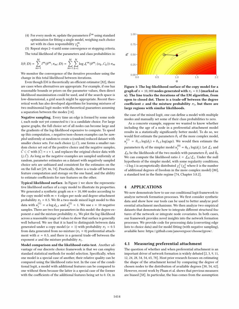
Figure 4: The log-likelihood of varying the class probabil-ities of the copy model (r = 1, p free) or the local searchmodel (r free, p = 1) for two different synthetic graphs. Inboth cases the true model is the most likely. On the left wesee a large difference in the log-likelihood between optima,while on the rightwe see a smaller difference. In both cases alikelihood ratio test is highly significant (P-values < 10−16).
To summarize, it is not recommended to estimate a formationmodel from an observed degree distribution. The parameter esti-mates are sensitive to small deviations in the generative process.Discrete choice modeling. Beyond degree distributions, in Fig-ure 4 we look at how the two subsumed models (the copy modeland the Jackson-Rogers local search model) fare when estimatedfrom formation data generated by the (r ,p)-model. We look at twocases. As a first case, we generate graphs with r = 0.5 and p = 1,so half the edges are formed to friends-of-friends with no utilityfrom degree. The likelihood under a local search model (r free,p = 1) as a mixed logit is maximized at r = 0.45, while for the copymodel (r = 1, p free) it is maximized at p = 0.54. The former isa much better fit than the latter (P-value < 10−16), and the copymodel erroneously thinks that preferential attachment is driving45% of the edges. As a second case, we look at a graph generatedwith r = 1 and p = 0.5, so half the edges are due to preferentialattachment, and friend-of-friending plays no role. In this case, bothmodels are correctly maximized at their relative values. Again, thecorrect model has a higher likelihood (P-value < 10−16).
4.3 Choosing to follow on FlickrWe now apply our framework to examine a real-world networkformation dataset capturing the growth of the Flickr social network.We find that incorporating a Friend-of-Friend feature beyond pref-erential attachment and link-reciprocation features substantiallyimproves both likelihood and test accuracy and furthermore thatthe inclusion of this feature significantly reduces preference fordegree-based attachment. However, omitting preferential attach-ment entirely leads to a worse model. We also find a preference fornodes with zero degree over low degree nodes. This hints that suchnodes play a special role in the network formation process, eventhough they would be ignored in preferential attachment models.Data. We use a scrape of the Flickr social network collected dailybetween October 2006 and May 2007 [50, 51]. Users of Flickr canchoose to follow other users and the “following” (but not the “fol-lowed by”) connections are publicly accessible. The data was gath-ered using a breadth-first search crawl, which means that only the
Table 3: Conditional logit model fits for Flickr data. Stan-dard errors of the estimates are given in parentheses. Eval-uation statistics are computed over 2,000 sampled examplesexcluded from the training data.
Model
#1 #2 #3 #4
log Followers 1.149* 0.715* 0.536*(0.007) (0.009) (0.010)
Has degree -0.580* -0.631* -1.745*(0.202) (0.190) (0.234)
Reciprocal 8.419* 8.347* 8.197* 7.903*(0.220) (0.220) (0.240) (0.244)
Is FoF 6.12* 3.955*(0.045) (0.050)
2 Hops 6.290*(0.190)
3 Hops 2.851*(0.185)
4 Hops 0.583*(0.189)
5 Hops -0.585*(0.218)
≥ 6 Hops -1.122*(0.266)
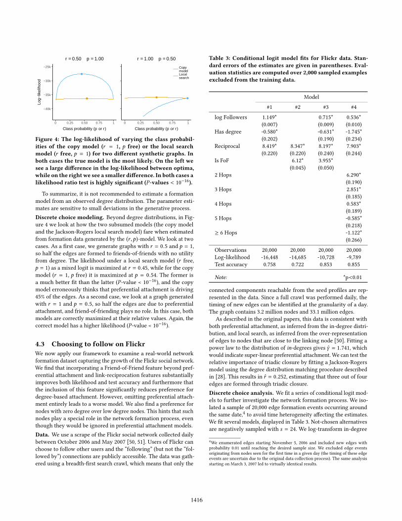
Observations 20,000 20,000 20,000 20,000Log-likelihood -16,448 -14,685 -10,728 -9,789Test accuracy 0.758 0.722 0.853 0.855
Note: *p<0.01
connected components reachable from the seed profiles are rep-resented in the data. Since a full crawl was performed daily, thetiming of new edges can be identified at the granularity of a day.The graph contains 3.2 million nodes and 33.1 million edges.
As described in the original papers, this data is consistent withboth preferential attachment, as inferred from the in-degree distri-bution, and local search, as inferred from the over-representationof edges to nodes that are close to the linking node [50]. Fitting apower law to the distribution of in-degrees gives γ̂ = 1.741, whichwould indicate super-linear preferential attachment. We can test therelative importance of triadic closure by fitting a Jackson-Rogersmodel using the degree distribution matching procedure describedin [28]. This results in r̂ = 0.252, estimating that three out of fouredges are formed through triadic closure.Discrete choice analysis. We fit a series of conditional logit mod-els to further investigate the network formation process. We iso-lated a sample of 20,000 edge formation events occurring aroundthe same date,4 to avoid time heterogeneity affecting the estimates.We fit several models, displayed in Table 3. Not-chosen alternativesare negatively sampled with s = 24. We log-transform in-degree
4We enumerated edges starting November 5, 2006 and included new edges withprobability 0.01 until reaching the desired sample size. We excluded edge eventsoriginating from nodes seen for the first time in a given day (the timing of these edgeevents are uncertain due to the original data collection process). The same analysisstarting on March 3, 2007 led to virtually identical results.
1416

(representing the number of followers), but in order to account fornodes with degree zero, we add a “has degree” feature for having apositive degree and use a modified version of log that returns 0 forinput 0.5 In the first column, we fit a model using just these twodegree-related features, and a reciprocity feature capturing whetherthe target node is already following the chooser. Reciprocity is acommon phenomenon, with 60% of edges being followed back [50].The estimate α̂ (the coefficient for “log Followers”) for this modelis significantly larger than 1, again consistent with super-linearpreferential attachment.
In the second model, we test the effect of the target node beinga friend-of-friend of the choosing node. In the case of Flickr, thismeans that the choosing user already follows someone that followsthe target user, which evidently is strongly correlated with follow-ing that user. However, combining these two features in a thirdmodel (column 3) leads to both estimated parameters droppingsubstantially. Most remarkable is the 40% drop in the estimate of α ,which paints a very different picture about the role of degree.
In the fourth model, we measure network proximity as in theoriginal paper, by counting the number of “hops” (path length)from i to the target before an edge was made. We integrate thehops as categorical variables to show the relative impact of eachadditional “hop”. Being two hops away is equivalent to being afriend-of-friend, and thus has strongly positive coefficient. Everyadditional hop corresponds to a sharp decrease in choosing thatnode. Being five hops away is slightly worse than there not beinga path at all. This could be an artifact of the way the data wasgathered, so that new regions of the graph only get “discovered”when there is at least one link to them, or this could be due to pathlength not being an accurate measure of distance for newer nodes.Since the number of hops is co-linear with being a friend-of-friend,we can’t test them both at the same time.
In Figure 5 we visually show the effect of different specifica-tions on the estimate of α̂ . The first model of the Flickr data lookslike super-linear preferential attachment, while the role of degreein the other two is significantly reduced. However, fitting a non-parametric model shows that the estimated coefficients for individ-ual degrees are remarkably linear, suggesting that the functionalform of dαj is a good fit for this network. One important point isthe role of zero-degree nodes. In most descriptions of preferentialattachment, nodes with degree zero are not considered. However,in the Flickr data set, zero-degree nodes have a higher utility thanpositive low degree nodes, which could again be an artifact of thedata collection process, or point to the special role of new nodes inthe network. Either way, our framework allows one to find thesekinds of patterns, and investigate them further.
4.4 Choosing to citeWe now turn to citation network data to show how a discrete choiceframework facilitates the testing of network formation hypotheses.Previous analyses of citation networks have observed linear pref-erential attachment with respect to degree [62] and bias towardsciting more recent work [62]. Here, we find consistent results that
5This solution is better than using logd + ϵ , or giving degree-zero nodes the sameutility as degree-one nodes. Either of those solutions will give substantially differentresults, especially when there are many degree-zero nodes.
●
●
●
●
●●
● ●
● ●
●●●
●●
●●●
●
●●
●
●●●
●●●●●
●
●●●●
●●●
●
●
●
●●●
●●●
●
●
●●●●●●
●
●●
●●
●
●
●
●
●
●●●
●
●
●
●
●
●●●●
●
●
●
●●
●
●●●●●●●●
●●●●●
●
●
●
●
●
●●
●
● ●● ●
●●●
●●●
●
●
●
●●
●
●●●
●●●
●
●●
●
●●
●
●
●●
●●
●
●●●
●
●●●●●●
●
●
●
●
●
●●
●
●
●
●
●
●
●●●
●●●
●●
●
●
●●
●●
●
●
●
●
●
●
●
●
●
●
●●
●
●
●
●
●●●
●●●●
●
●
●
● ● ●
● ● ● ●
●●●
●●●
●
●
●
●●
●
●●●
●●●
●
●●
●
●●
●
●
●●
●●●
●●●●
●●●●●●
●
●
●
●
●
●●
●
●
●
●
●
●
●●●●●●
●●
●
●
●●
●●
●
●
●
●
●
●
●
●
●
●
●
●
●
●
●
●●●●
●●●●
●●
●
100
101
102
0 100 101 102
Degree
Rel
ativ
e P
roba
bilit
y
3.1
3.3
3.4
Flickr
●
●
●
● ●●
● ● ● ●●
●●●
●●●
●●●●●
●●●●●
●
●●●●●●
●●●
●
●●●●●●
●●●
●●●●●●
●
●●●●●●●
●●
●●●
●
●
●
●
●●
●
●
●
●●
●
●●●●●
●
●
●●
●●
●
●●●
●
●●●●●
●
●
●
●
●
●●
●
● ●●
●● ●●●
●●●●●
●
●●●●
●
●●●
●●
●●
●●●●
●
●
●●●●●
●
●
●
●●●●
●●
●
●
●
●
●●●●
●
●
●
●●●
●
●
●
●
●●●●
●
●●
●●●
●●●
●
●
●●
●●
●●●
●
●
●●
●
●●
●
●
●
●
0 100 101 102
Degree
4.1
4.3
Citations
Figure 5: The probability of being chosen by degree, as com-pared to a nodewith degree 1.We show the fits of parametric(lines) and non-parametric (points) conditional logit modelsof the Flickr and citation networks. The legend referencesmodel numbers in Table 3 and Table 4. The estimate for de-gree 0 is inserted for comparison. Dashed reference lines il-lustrate what exact linear preferential attachment (α = 1)would look like.
older papers are less likely to be cited but that accounting for ageactually increases the importance of degree (i.e., after accountingfor age, higher degree nodes are more likely to be cited).Data. We use the Microsoft Academic Graph6 dataset and focuson a representative subgraph of 459,000 “Climatology” papers. Wefocus on the subgraph of a single field to simplify the analysis sincecitations are predominantly within the same field of study (ouranalysis was similar on other subgraphs). We construct a graphout of this data by adding an edge each time a paper in our datasetcites another paper in our dataset. For our analysis of Climatologypublications, 45% of edges are within the domain and citations topapers that are not labeled are excluded, leaving 3 million edges.We sample 10,000 citation events uniformly at random from paperspublished after 2010 and apply negative sampling (s = 24). Thisprocessing results in 10,000 choices with 25 alternatives in eachchoice set. For each possible choice, we compute four features: thenumber of citations at the time of citation, whether the paper sharesauthors with the citing paper, the age of the paper in years at thetime of citation, and the maximum number of publications by anyone of the authors at the time of publication. This last feature is aproxy for node fitness [11].Discrete choice analysis. We fit conditional logit choice modelsrelating these features to the likelihood of citation (Table 4). Thefirst model (first column) is a simple log-degree model. We find thatthe estimate α̂ (the coefficient for “log Citations”) is substantiallylower than one, consistent with sub-linear preferential attachment.Apart from the log-likelihood of the models, we also report thepredictive accuracy (defined as the share of instances predictedcorrectly) on a holdout test set of 2,000 examples. Just relying onprior degree already gives an accuracy of 36%, which is high for aclassification task with 25 classes. In model two (second column),we add a covariate for whether a paper shares an author with theciting paper. As expected, this has a strongly positive coefficient.
For the third model we add a covariate for the age of the pa-per in log years (years is always at least one). Older papers are
6The Aminer Project [68, 72], https://aminer.org/open-academic-graph
1417

Table 4: Learned conditional logits for the “Climatology” ci-tation network. Standard errors of the estimates are given inparentheses. Evaluation statistics are computed over 2,000sampled examples excluded from the training data.
Model
#1 #2 #3 #4
log Citations 0.717* 0.794* 1.052* 1.044*(0.008) (0.010) (0.012) (0.012)
Has degree 1.684* 1.677* 1.862* 1.830*(0.053) (0.062) (0.063) (0.064)
Has same author 6.523* 5.928* 5.913*(0.110) (0.114) (0.114)
log Age -1.096* -1.069*(0.018) (0.021)
Max papers by author 0.029*(0.011)
Observations 10,000 10,000 10,000 10,000Log-likelihood -20,799 -16,600 -14,384 -14,390Test accuracy 0.358 0.484 0.533 0.534
Note: *p<0.01
less likely to get cited (accounting for degree), but accounting forage increases the relative importance of degree significantly. Thisexpanded model also increases the accuracy to 53%, indicatingthat these feature weights do capture substantially more predictivepower. Finally, in model four we add the “max papers by authors”feature as a proxy for fitness. The coefficient is small but positive.Accounting for fitness slightly reduces the estimated relative im-portance of degree, but the α̂ estimate is still close to 1. Addingthis feature does not improve the log-likelihood or predictive accu-racy; a better proxy for fitness may explain the data better. Lookingback to the visual display of α for the citation models in Figure5, the non-parametric coefficients are highly linear. In this data,zero-degree nodes are significantly less attractive than nodes withdegree one.
As with any regression, the identifying causal effects frommodelfit depends on the design of the study. The estimates we providehere, as is the case with most analyses of observational data, aredescriptive and not meant to describe causal processes. The point isthat discrete choice models provide a flexible framework to easilytest and compare different hypotheses around network formation.
5 DISCUSSIONWhen modeling network formation, the majority of the literatureanalyzes networks that grow “externally,” with new nodes arrivingand choosing who to connect to, and this setting has also been ourmain focus here. External growth leads to convenient models thatare relatively easy to analyze, with citation networks and patentnetworks as examples of empirical networks that follow this gen-erative process reasonably closely. However, in many (especiallysocial) networks, pairs of older nodes often form edges as well,edges that are “internal” to the existing set of nodes. An extremeexample is the social networks of schools or classrooms, which
have a fixed node population and “grow” purely through an in-ternal growth process. A major advantage of modeling networkformation as discrete choice is that it does not require any modelof edge event initiation and simply conditions on the sequence ofdecisions to initiate, focusing the modeling on the choices made bythe initiator. Discrete choice can therefore easily be used to modelinternal growth as well.
Another major advantage of discrete choice modeling is that itconnects the analysis of large-scale network datasets to statisticalmethods (fitting generalized linear models) that are tremendouslyscalable. As we show in this work, additional techniques (e.g., neg-ative sampling) makes it possible to efficiently scale the estimationprocess to very large network datasets.
Since the conditional logit model of discrete choice is a randomutility model, the estimated parameters can be interpreted as themarginal utility of each feature. This allows one to question thefunctional form of features. For example, we show that preferentialattachment is equivalent to the logarithmic utility of degree. Giventhat degree is commonly heavy-tailed, this is a natural functionalform, but we point out that the conditional logit allows one toflexibly compare different specifications.
Our discrete choice perspective has implications for hownetworkdata is best collected and analyzed. It is useful to consider and recordnotions of directionality, even if edges can otherwise be consideredto be undirected. With information about the choice set associatedwith each choice, we can see what each node j looked like at thetime the choice was made. Datasets that record the exact time of alledge formation events, as opposed to lumping edge events at thegranularity of days or years, makes it possible to further analyzethe formation process in more detail.
There are a couple limitations to our proposed methodology.First, we cannot model purely undirected edges without some no-tion of direction. Second, even though the conditional logit andmixed logit models allow one to model similar mechanisms, theinterpretations of their estimates are different. The estimates of aconditional logit are more akin to those of a linear regression model,where one estimates the expected change in an outcome from vary-ing a covariate. A mixture model is a probabilistic combination ofconstituent modes, so the class probabilities indicate the relativeimportance to each mode, which makes it harder to compare theroles of individual features within or across modes. However, manytraditional models of network formation are equivalent to mixturemodels, which motivated our consideration of them in this work.
By making foundational connections between network forma-tion and discrete choice, we are hopeful that many further toolsfrom discrete choice theory can be applied to the study of networkformation. For example, there can be bias in network formation, e.g.,men are more likely to cite themselves than women [34]. Our dis-crete choice framework can help study these cases more rigorously.For another example, discrete choice models of subset selection[5, 20] could be applied to understand possible substitution andcomplementarity effects in network formation. And discrete choiceinterpretations of machine learning embeddings techniques [64]can likely help unpack the behavior of recent embedding-basednetwork representation methods such as DeepWalk [57]. Networksfundamentally represent interactions between discrete entities, and
1418

it is therefore natural that methods for modeling and analyzingdiscrete choice should enable many contributions.Acknowledgements. We thank Aaron Clauset, Eduardo Laguna-Müggenburg, and Daniel Larremore for their helpful comments andfeedback. ARB was supported by NSF Award DMS-1830274 andARO award 86798. JO and JU were supported in part by an AROYoung Investigator Award.
REFERENCES[1] Alan Agresti. 2003. Categorical data analysis. Vol. 482. John Wiley & Sons.[2] Réka Albert and Albert-László Barabási. 1999. Emergence of scaling in random
networks. Science 286, 5439 (1999), 509–512.[3] James P Bagrow and Dirk Brockmann. 2013. Natural Emergence of Clusters and
Bursts in Network Evolution. Physical Review X 3, 2 (2013).[4] Austin R Benson, Ravi Kumar, and Andrew Tomkins. 2016. On the relevance of
irrelevant alternatives. In WWW. ACM, 963–973.[5] Austin R Benson, Ravi Kumar, and Andrew Tomkins. 2018. A Discrete Choice
Model for Subset Selection. In WSDM. ACM, 37–45.[6] Ginestra Bianconi and Albert-László Barabási. 2001. Bose-Einstein condensation
in complex networks. Physical review letters 86, 24 (2001).[7] Ginestra Bianconi and A-L Barabási. 2001. Competition and multiscaling in
evolving networks. EPL (Europhysics Letters) 54, 4 (2001), 436.[8] Béla Bollobás and Oliver M Riordan. 2003. Mathematical results on scale-free
random graphs. Handbook of graphs and networks: from the genome to the internet(2003), 1–34.
[9] Anna D Broido and Aaron Clauset. 2018. Scale-free networks are rare. arXivpreprint arXiv:1801.03400 (2018).
[10] Carter T Butts. 2008. A Relational Event Framework for Social Action. SociologicalMethodology 38, 1 (2008), 155–200.
[11] Guido Caldarelli, Andrea Capocci, Paolo De Los Rios, and Miguel A Munoz. 2002.Scale-free networks from varying vertex intrinsic fitness. Physical Review Letters89, 25 (2002), 258702.
[12] Duncan S Callaway, John E Hopcroft, Jon M Kleinberg, Steven H Strogatz, andMark E J Newman. 2001. Are randomly grown graphs really random? PhysicalReview E 64, 4 (2001).
[13] Sourav Chatterjee and Persi Diaconis. 2013. Estimating and understandingexponential random graph models. Annals of Statistics 41, 5 (2013), 2428–2461.
[14] Flavio Chierichetti, Ravi Kumar, and Andrew Tomkins. 2018. Learning a mixtureof two multinomial logits. In ICML. PMLR, 961–969.
[15] Aaron Clauset, Cristopher Moore, and Mark E J Newman. 2008. Hierarchicalstructure and the prediction of missing links in networks. Nature 453, 7191 (2008),98–101.
[16] Aaron Clauset, Cosma R Shalizi, and Mark E J Newman. 2009. Power-LawDistributions in Empirical Data. SIAM Rev. 51, 4 (Dec. 2009), 661–703.
[17] Colin Cooper and Alan Frieze. 2003. A general model of web graphs. RandomStructures & Algorithms 22, 3 (2003), 311–335.
[18] Arthur P Dempster, NanM Laird, and Donald B Rubin. 1977. Maximum likelihoodfrom incomplete data via the EM algorithm. Journal of the royal statistical society.Series B (1977), 1–38.
[19] David Easley and Jon Kleinberg. 2010. Networks, crowds, and markets: Reasoningabout a highly connected world. Cambridge University Press.
[20] Peter C Fishburn and Irving H LaValle. 1996. Binary interactions and subsetchoice. European Journal of Operational Research 92, 1 (1996), 182–192.
[21] Winship C Fuller, Charles F Manski, and David A Wise. 1982. New evidenceon the economic determinants of postsecondary schooling choices. Journal ofHuman Resources (1982), 477–498.
[22] Peter D Hoff, Adrian E Raftery, and Mark S Handcock. 2002. Latent space ap-proaches to social network analysis. Journal of the american Statistical association97, 460 (2002), 1090–1098.
[23] Paul W Holland, Kathryn Blackmond Laskey, and Samuel Leinhardt. 1983. Sto-chastic blockmodels: First steps. Social networks 5, 2 (1983), 109–137.
[24] Petter Holme and Beom Jun Kim. 2002. Growing scale-free networks with tunableclustering. Physical review E 65, 2 (2002).
[25] Petter Holme and Jari Saramäki. 2012. Temporal networks. Physics reports 519, 3(2012), 97–125.
[26] Samuel Ieong, Nina Mishra, and Or Sheffet. 2012. Predicting preference flips incommerce search. In ICML. PMLR, 1795–1802.
[27] Kansuke Ikehara and Aaron Clauset. 2017. Characterizing the structural diversityof complex networks across domains. arXiv preprint arXiv:1710.11304 (2017).
[28] Matthew O Jackson and Brian W Rogers. 2007. Meeting Strangers and Friends ofFriends: How Random Are Social Networks? American Economic Review 97, 3(2007), 890–915.
[29] Benjamin F Jarvis. 2018. Estimating Multinomial Logit Models with Samples ofAlternatives. Sociological Methodology (2018).
[30] H Jeong, Z Neda, and Albert-László Barabási. 2003. Measuring preferentialattachment in evolving networks. Europhysics Letters (EPL) 61, 4 (2003), 567–572.
[31] Emily M Jin, Michelle Girvan, and Mark EJ Newman. 2001. Structure of growingsocial networks. Physical Review E 64, 4 (2001), 046132.
[32] Wagner A Kamakura and Gary J Russell. 1989. A probabilistic choice model formarket segmentation and elasticity structure. Journal of mMrketing Research(1989), 379–390.
[33] Brian Karrer and Mark EJ Newman. 2011. Stochastic blockmodels and communitystructure in networks. Physical review E 83, 1 (2011), 016107.
[34] Molly M King, Carl T Bergstrom, Shelley J Correll, Jennifer Jacquet, and Jevin DWest. 2017. Men set their own cites high: Gender and self-citation across fieldsand over time. Socius 3 (2017).
[35] Jon M Kleinberg, Ravi Kumar, Prabhakar Raghavan, Sridhar Rajagopalan, andAndrew S Tomkins. 1999. The web as a graph: measurements, models, andmethods. In International Computing and Combinatorics Conference. Springer,1–17.
[36] Paul L Krapivsky, Sidney Redner, and Francois Leyvraz. 2000. Connectivity ofgrowing random networks. Physical review letters 85, 21 (2000), 4629.
[37] Dmitri Krioukov, Fragkiskos Papadopoulos, Maksim Kitsak, Amin Vahdat, andMarián Boguná. 2010. Hyperbolic geometry of complex networks. PhysicalReview E 82, 3 (2010), 036106.
[38] Ravi Kumar, Jasmine Novak, and Andrew Tomkins. 2010. Structure and evolutionof online social networks. In Link mining: models, algorithms, and applications.Springer, 337–357.
[39] Ravi Kumar, Prabhakar Raghavan, Sridhar Rajagopalan, D Sivakumar, AndrewTomkins, and Eli Upfal. 2000. Stochastic models for the web graph. In Proceedingsof the 42st Annual Symposium on Foundations of Computer Science. IEEE, 57–65.
[40] Jure Leskovec, Lars Backstrom, Ravi Kumar, and Andrew Tomkins. 2008. Micro-scopic evolution of social networks. In KDD. ACM, 462–470.
[41] Jure Leskovec, Jon M Kleinberg, and Christos Faloutsos. 2007. Graph evolution:Densification and shrinking diameters. Transactions on Knowledge Discoveryfrom Data (TKDD) 1, 1 (2007).
[42] David Liben-Nowell and Jon Kleinberg. 2007. The link-prediction problem forsocial networks. Journal of the American society for information science andtechnology 58, 7 (2007), 1019–1031.
[43] Zonghua Liu, Ying-Cheng Lai, Nong Ye, and Partha Dasgupta. 2002. Connectivitydistribution and attack tolerance of general networks with both preferential andrandom attachments. Physics Letters A 303, 5-6 (2002), 337–344.
[44] Linyuan Lü and Tao Zhou. 2011. Link prediction in complex networks: A survey.Physica A: Statistical Mechanics and its Applications 390, 6 (2011), 1150–1170.
[45] R Duncan Luce. 1959. Individual Choice Behavior; a Theoretical Analysis. NewYork: Wiley.
[46] Daniel McFadden. 1978. Modeling the choice of residential location. Transporta-tion Research Record 673 (1978).
[47] Daniel McFadden et al. 1973. Conditional logit analysis of qualitative choicebehavior. (1973).
[48] Miller McPherson, Lynn Smith-Lovin, and James M Cook. 2001. Birds of a feather:Homophily in social networks. Annual review of sociology 32, 1 (2001), 19–28.
[49] Jan Medina, Jorge Finke, and Camilo Rocha. 2018. Estimating Formation Mecha-nisms and Degree Distributions in Mixed Attachment Networks. arXiv.org (2018).arXiv:math.PR/1809.03372v1
[50] Alan Mislove, Hema Swetha Koppula, Krishna P Gummadi, Peter Druschel, andBobby Bhattacharjee. 2008. Growth of the Flickr Social Network. In Proceedingsof the 1st SIGCOMM Workshop on Social Networks.
[51] Alan Mislove, Massimiliano Marcon, Krishna P Gummadi, Peter Druschel, andBobby Bhattacharjee. 2007. Measurement and analysis of online social networks.In Proceedings of the 7th SIGCOMM conference on Internet Measurement. ACM.
[52] Michael Mitzenmacher. 2003. A Brief History of Generative Models for PowerLaw and Lognormal Distributions. Internet Mathematics 1, 2 (2003), 226–251.
[53] Rajeev Motwani and Ying Xu. 2006. Evolution of page popularity under randomweb graph models. In PODS. ACM, 134–142.
[54] Mark E J Newman. 2001. Clustering and preferential attachment in growingnetworks. Physical Review E 64, 2 (2001), 440–4.
[55] Fragkiskos Papadopoulos, Maksim Kitsak, M Ángeles Serrano, Marián Boguná,and Dmitri Krioukov. 2012. Popularity versus similarity in growing networks.Nature 489, 7417 (2012), 537.
[56] Ashwin Paranjape, Austin R Benson, and Jure Leskovec. 2017. Motifs in temporalnetworks. InWSDM. ACM, 601–610.
[57] Bryan Perozzi, Rami Al-Rfou, and Steven Skiena. 2014. Deepwalk: Online learningof social representations. In KDD. ACM, 701–710.
[58] Thong Pham, Paul Sheridan, and Hidetoshi Shimodaira. 2015. PAFit: A StatisticalMethod for Measuring Preferential Attachment in Temporal Complex Networks.PLoS ONE 10, 9 (2015).
[59] Derek de Solla Price. 1976. A general theory of bibliometric and other cumulativeadvantage processes. Journal of the American Society for Information Science 27,5 (1976), 292–306.
[60] Stephen Ragain and Johan Ugander. 2016. Pairwise choice Markov chains. InNIPS. 3198–3206.
1419

[61] Anatol Rapoport. 1953. Spread of information through a population with socio-structural bias: I. Assumption of transitivity. The bulletin of mathematical bio-physics 15, 4 (1953), 523–533.
[62] Sidney Redner. 2005. Citation Statistics from 110 Years of Physical Review. PhysicsToday 58, 12 (2005).
[63] Garry Robins, Pip Pattison, Yuval Kalish, and Dean Lusher. 2007. An introductionto exponential random graph (p*) models for social networks. Social networks 29,2 (2007), 173–191.
[64] Maja Rudolph, Francisco Ruiz, Stephan Mandt, and David Blei. 2016. Exponentialfamily embeddings. In NIPS. 478–486.
[65] Jari Saramäki and Kimmo Kaski. 2004. Scale-free networks generated by randomwalkers. Physica A: Statistical Mechanics and its Applications 341 (2004), 80–86.
[66] Cosma R Shalizi and Alessandro Rinaldo. 2013. Consistency under sampling ofexponential random graph models. Annals of Statistics 41, 2 (2013), 508–535.
[67] Itamar Simonson and Amos Tversky. 1992. Choice in context: Tradeoff contrastand extremeness aversion. Journal of Marketing Research 29, 3 (1992), 281.
[68] Arnab Sinha, Zhihong Shen, Yang Song, Hao Ma, Darrin Eide, Bo-june Paul Hsu,and Kuansan Wang. 2015. An overview of microsoft academic service (mas) andapplications. In WWW. ACM, 243–246.
[69] Tom AB Snijders. 2001. The Statistical Evaluation of Social Network Dynamics.Sociological Methodology 31, 1 (2001), 361–395.
[70] Tom AB Snijders, Gerhard G Van de Bunt, and Christian EG Steglich. 2010.Introduction to stochastic actor-based models for network dynamics. Socialnetworks 32, 1 (2010), 44–60.
[71] Christoph Stadtfeld, James Hollway, and Per Block. 2017. Dynamic Network ActorModels: Investigating Coordination Ties through Time. Sociological Methodology47, 1 (2017), 1–40. https://doi.org/10.1177/0081175017709295
[72] Jie Tang, Jing Zhang, Limin Yao, Juanzi Li, Li Zhang, and Zhong Su. 2008. Ar-netminer: extraction and mining of academic social networks. In KDD. ACM,990–998.
[73] Kenneth E Train. 2008. EM algorithms for nonparametric estimation of mixingdistributions. Journal of Choice Modelling 1, 1 (2008), 40–69.
[74] Kenneth E Train. 2009. Discrete choice methods with simulation. Cambridgeuniversity press.
[75] Kenneth E Train and Daniel McFadden. 1978. The goods/leisure tradeoff anddisaggregate work trip mode choice models. Transportation research 12, 5 (1978),349–353.
[76] Amos Tversky. 1972. Elimination by aspects: A theory of choice. PsychologicalReview 79, 4 (1972), 281.
[77] Johan Ugander, Brian Karrer, Lars Backstrom, and Cameron Marlow. 2011. Theanatomy of the facebook social graph. arXiv preprint arXiv:1111.4503 (2011).
[78] Alexei Vázquez. 2003. Growing network with local rules: Preferential attachment,clustering hierarchy, and degree correlations. Physical Review E 67, 5 (2003).
[79] Stanley Wasserman and Philippa Pattison. 1996. Logit models and logistic re-gressions for social networks: I. An introduction to Markov graphs and p*. Psy-chometrika 61, 3 (1996), 401–425.
[80] Samuel S Wilks. 1938. The large-sample distribution of the likelihood ratiofor testing composite hypotheses. Annals of Mathematical Statistics 9, 1 (1938),60–62.
[81] CarstenWiuf, Markus Brameier, Oskar Hagberg, and Michael PH Stumpf. 2006. Alikelihood approach to analysis of network data. PNAS 103, 20 (2006), 7566–7570.
[82] Lei Xu and Michael I Jordan. 1996. On Convergence Properties of the EMAlgorithm for Gaussian Mixtures. Neural Computation 8, 1 (1996), 129–151.
1420