chromatic dispersion at high bit rates - ccontrols.ch · this pocket guide provides a comprehensive...

Chromatic Dispersion at High Bit Rates

This pocket guide provides a comprehensive view of chromatic dispersion from concept to testing

A lot of time, effort and money have gone into dealing with chromatic dispersion. But why? And what does the future hold as demand and bit rates continue to increase exponentially?

Let’s face it, sometimes it’s hard to keep up on the latest trends and solutions, especially when components are always improving, fiber types are diversifying and receivers and transmitters are constantly evolving. This is what this guide is for.

This guide explores the concerns and costs of chromatic dispersion. It reviews the different transmission formats, compensation schemes as well as the impact and limitations of various fiber types, transmission techniques and bit rates. Finally, the guide also reviews the most common testing techniques on the market and sheds light on Raman amplifier deployment.

EXFO Chromatic Dispersion at High Bit Rates 1

Table of contents1. Dispersion-related transmission impairments ............. 2

2. Defining the dispersion phenomenon ........................... 4

3. Transmitter source characteristics ................................ 5

4. Fiber-dispersion specifications ...................................... 6

5. Pulse broadening due to chromatic dispersion ..........12 5.1 Maximum allowed dispersion ........................................................ 11

5.2 Maximum reachable distance ....................................................... 14

6. Dispersion impairment and compensation .................16 6.1 Dispersion compensation .............................................................. 19

6.2 Dispersion-compensating fiber in a WDM system ..................... 20

6.3 Maximum CD deviation ................................................................... 23

6.4 WDM systems: tolerance to residual CD ...................................... 24

7. Modulation and its influence on chromatic dispersion .........................................................................25

7.1 Modulator influence ........................................................................ 25

7.2 NRZ-OOK modulation format .......................................................... 26

7.3 RZ-OOK modulation format ........................................................... 27

7.4 PSK modulation format ................................................................... 28

7.5 Variation in the phase-shift keying modulation technique – NRZ-DPSK modulation format ........................................................ 30

7.6 Variation in the phase-shift keying modulation technique – Carrier-suppressed RZ modulation ............................................... 31

7.7 Variation in the phase-shift keying modulation technique – Duo-binary modulation format ...................................................... 32

8. Chromatic dispersion measurement ...........................37 8.1 Data fitting ........................................................................................ 38

8.2 CD test methods .............................................................................. 39

8.2.1 Test method – General requirements .............................. 40

8.2.2 Phase-shift method ............................................................. 40

8.2.3 An improvement to the phase-shift method for field testing ..................................................................... 43

8.2.4 Differential phase-shift method (DPSM) .......................... 45

8.2.5 Spectral group delay in the time domain method .......... 46

9. Chromatic dispersion testing in coherent systems ...51 9.1 Raman gain ....................................................................................... 52

9.2 Knowing the Effective Area ............................................................ 53

9.3 CD Testing ......................................................................................... 54

2 EXFO Chromatic Dispersion at High Bit Rates

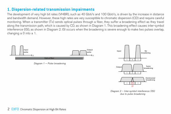
1. Dispersion-related transmission impairmentsThe development of very high bit rates (VHBR), such as 40 Gbit/s and 100 Gbit/s, is driven by the increase in distance and bandwidth demand. However, these high rates are very susceptible to chromatic dispersion (CD) and require careful monitoring. When a transmitter (Tx) sends optical pulses through a fiber, they suffer a broadening effect as they travel along the transmission path, which is caused by CD, as shown in Diagram 1. This broadening effect causes inter-symbol interference (ISI), as shown in Diagram 2. ISI occurs when the broadening is severe enough to make two pulses overlap, changing a 0 into a 1.

Inputpulse

Optical �ber

Outputpulse

t t

Diagram 1 − Pulse broadening

ISI

Nobroadening

1 10

Somebroadening

Detrimentalbroadening

Input

Output

1 10

1 11

Diagram 2 – Inter-symbol interference (ISI) due to pulse broadening


One way to improve CD performance, as shown in Diagram 3, is through a shorter duty cycle (i.e., shorter pulse duration within the bit period), but it comes at a price: widening the signal spectrum lowers the average pulse power that in turn worsens the optical signal to noise ratio (OSNR). Pulse power must therefore be increased to maintain the same OSNR. However, this may lead to nonlinear effects (NLE), which are particularly sensitive to high power.

NRZ

RZ (2/3 NRZ) (same pulse energy as NRZ)



1 0 0 1 1 1 0 1

1 0 0 1 1 1 0 1

1 0 0 1 1 1 0 1

1 0 0 1 1 1 0 1

NRZ



1 0 0 1 1 1 0 1

1 0 0 1 1 1 0 1

1 0 0 1 1 1 0 1

1 0 0 1 1 1 0 1


Diagram 3 – Optical pulses and corresponding bit stream for NRZ and RZ formats (constant pulse energy)

(a) No broadening (b) Dispersion-impaired pulse broadening from (a)


2. Defining the dispersion phenomenonThere are three types of dispersion:

› Intermodal or multimode dispersion

› Intramodal or single-mode chromatic dispersion (CD) › Material dispersion › Waveguide dispersion

› Polarization mode dispersion (PMD)

Chromatic dispersion is illustrated in Diagram 4. The consequence is very straightforward: the input pulse of information broadens as it is travels through the optical fiber or other dispersive medium.

Of the three types of dispersion, with respect to single-mode fiber (SMF) transmission, CD causes the most impairment, whereas PMD is the most difficult to predict and resolve. The former is described as a deterministic phenomenon; the latter is a stochastic phenomenon.

Chromatic dispersion occurs because different optical wavelengths/frequencies launched from the Tx light source travel at different velocities in a propagating dispersive medium.

Inputpulse

Core

Cladding

time, distance

Broadenedpulse

Note: Different wavelengths (designated by different colors) of a modulated single-mode laser travel at different velocities inside a single-mode optical fiber.

Diagram 4 − Intramodal chromatic dispersion of a single-mode optical fiber


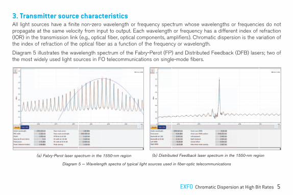
3. Transmitter source characteristicsAll light sources have a finite non-zero wavelength or frequency spectrum whose wavelengths or frequencies do not propagate at the same velocity from input to output. Each wavelength or frequency has a different index of refraction (IOR) in the transmission link (e.g., optical fiber, optical components, amplifiers). Chromatic dispersion is the variation of the index of refraction of the optical fiber as a function of the frequency or wavelength.

Diagram 5 illustrates the wavelength spectrum of the Fabry-Perot (FP) and Distributed Feedback (DFB) lasers; two of the most widely used light sources in FO telecommunications on single-mode fibers.

Diagram 5 − Wavelength spectra of typical light sources used in fiber-optic telecommunications

(a) Fabry-Perot laser spectrum in the 1550-nm region (b) Distributed Feedback laser spectrum in the 1550-nm region


The IOR is what makes source wavelengths not travel at the same velocity (group velocity) and arrive at different times at the end of the fiber. A pulse transmitted in such media suffers a spreading and dispersive effect, thus limiting the transmission bandwidth.

4. Fiber-dispersion specificationsThe change in wavelength velocities and, more importantly, the rate of that change (the CD itself) is not linear and, consequently, makes the pulse broadening more severe at some wavelengths than others. Tables 1 to 4 describe the specifications of the optical fibers used in FO telecommunications as defined in the ITU-T Recommendations.


Table 1 – Typical chromatic dispersion specifications on G.652, G.653 and G.654 optical fibers

ITU-T Recommandation G.652 G.653 G.654

Fiber Type Parameter A/B/C/D A B A B C

l0, min nm 1300 1500 -- -- -- -- --

l0, max nm 1324 1600 -- -- -- -- --

lmin nm -- 1525 -- -- -- -- --

lmax nm -- 1575 -- -- -- -- --

lrange nm -- -- 1460 – 1525 1525 – 1625 -- -- --

Dmin,lrange ps/nm-km -- -- [0.085•(l-1525)]-3.5 3.5•(l-1600)/75 -- -- --

lrange nm -- -- 1460 – 1575 1575 – 1625 1550

Dmin,lrange ps/nm-km -- -- 3.5•(l-1500)/75 [0.085•(l-1575)]+3.5 +20 +20 +20

S0,max ps/nm2-km 0.092 0.085 -- -- -- -- --

l(Smax) nm -- -- -- -- 1550

Smax ps/nm2-km -- -- -- 0.070

llink nm 1550 -- l0,typ = 1550 1550

Slink ps/nm2-km 0.056 -- S0,typ = 0.07 TBD

Dlink ps/nm-km +17 -- -- TBD


Table 2 – Typical chromatic dispersion specifications on G.655 optical fiber

ITU-T Recommandation G.655

Type Parameter A B/C

lrange nm 1530 – 1565 1565 – 1625

lmin nm 1530 TBD

lmax nm 1565 TBD

Dmin ps/nm-km Lower ±0.1 Lower ±0.1 Lower ±TBD

Dmax ps/nm-km Upper ±6.0 Upper ±10.0 Upper ±TBD

Dmin - Dmax ps/nm-km -- ≤ 5.0 --

llink, range nm -- -- --

Slink ps/nm2-km -- -- --

Dlink ps/nm-km -- -- --



Type Parameter D E

lrange nm 1460 – 1550 1550 – 1625 1460 – 1550 1550 – 1625

lmin nm -- -- -- --

lmax nm -- -- -- --

Dmin ps/nm-km [7.00•(l-1460)/90]-4.20 [2.97•(l-1550)/75]+2.80 [5.42•(l-1460)/90]+0.64 [3.30•(l-1550)/75]+6.06

Dmax ps/nm-km c [5.06•(l-1550)/75]+6.20 [4.65•(l-1460)/90]+4.66 [4.12•(l-1550)/75]+9.31

Dmin - Dmax ps/nm-km -- -- -- --

llink, range nmVarious implementations are possible, designed to optimize various tradeoffs in power, channel spacing,

amplifier separation, link length and bit rate. These implementations are primarily variations in the allowed CD, CD slope, and non-linear coefficient.

Slink ps/nm2-km

Dlink ps/nm-km



Parameter

lrange nm 1460 – 1550 1550 – 1625

Dmin ps/nm-km [2.60•(l-1460)/90]+1.00 [0.98•(l-1550)/75]+3.60

Dmax ps/nm-km [4.68•(l-1460)/90]+4.60 [4.72•(l-1550)/75]+9.28

llink, range nm 1460 1550 1625

Slink ps/nm2-km TBD TBD TBD

Dlink ps/nm-km -- TBD --


Fiber Type Parameter A B

l0, min nm 1300

TBDl0, min nm 1324

S0, max ps/nm2-km 0.092

Table 3 – ITU-T specifications for chromatic dispersion of G.656 optical fiber

Table 4 – Specifications for chromatic dispersion of G.657 optical fiber


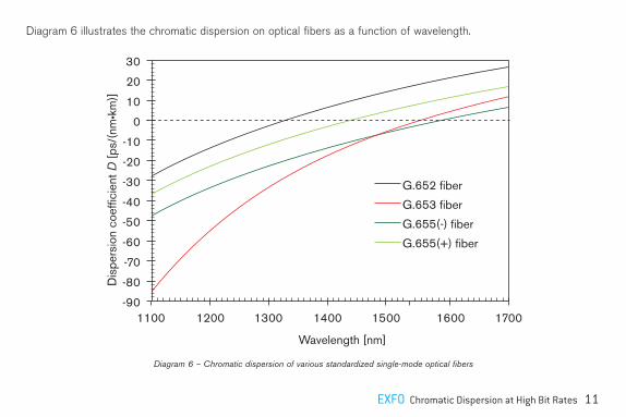
Diagram 6 illustrates the chromatic dispersion on optical fibers as a function of wavelength.

Diagram 6 – Chromatic dispersion of various standardized single-mode optical fibers

30

20

10

0

-10

-20

-30

-40

-50

-60

-70

-80

-901100

G.652 fiber

G.653 fiber

G.655(-) fiber

G.655(+) fiber

1200 1300 1400

Dis

pers

ion

coef

ficie

nt D

[ps/

(nm•k

m)]

Wavelength [nm]

1500 1600 1700


5. Pulse broadening due to chromatic dispersionFrom the Tx, the pulse broadening resulting from CD is caused by:

› The presence of different wavelengths in the optical spectrum of the light source. Each wavelength has a different IOR, which leads to a different phase delay and group delay along the fiber.

› The source modulation, which has two effects (broadening/compression): › Chirping occurs when the source wavelength spectrum varies during the pulse, especially at its rising and falling

edges. The wavelengths at the end of the pulse are delayed with respect to those at the beginning, which causes broadening. But if this delay is opposite to the fiber CD RGD, pulse compression can also occur. The chirp effect is described in Table 5.

Table 5 − Chirp effect on the dispersion and pulse broadening

Chromatic dispersion effects on the widths of both the source spectrum and the Tx modulation can be taken into account considering the following hypotheses: maximum allowed dispersion and maximum reachable distance.

Chirp signDirection of wavelength shift inside the pulse Sign effect of (chirp x dispersion) product

Pulse rise time Pulse decay time + –

+ Towards shorter wavelengths Towards longer wavelengths Pulse broadening Pulse compression to a minimum and broadening afterwards

– Towards longer wavelengths Towards shorter wavelengths Pulse compression to a minimum and broadening afterwards Pulse broadening


5.1 Maximum allowed dispersion

For every power penalty and BER, the tolerated ISI resulting from CD broadening has an upper limit. It is reached when the maximum pulse broadening equals a fraction of the input pulse bit period or time slot occupied by the pulse.

Table 6 – Maximum allowed dispersion for various NRZ pulse spectral widths and power penalties

In Table 6, the maximum tolerated dispersion increases with narrower NRZ pulse spectra, especially at low bit rates. At very high bit rates, the influence of the pulse spectral width dissipates because the maximum tolerated dispersion becomes extremely small. It’s at this point that residual dispersion and dispersion accommodation become very critical.

Power penalty [dB] 0.5 1 2

B [Gbit/s] (D•L)Max [ps/nm]

2.5 47126 18468 29731

10 794 1193 1920

40 50 75 120

100 8 12 19


5.2 Maximum reachable distance

When the dispersion of typical fibers is known, the above data can be used to compute maximum reachable distance.

Table 7 – Maximum reachable distance for various NRZ pulse spectral widths and fiber

LMax [km], PISI = 1 dB D(1565 nm) [ps/nm.km]

Fiber Type G.652 G.653 G.655

B [Gbit/s] 18.7 1.4 9

2.5 970 12940 2013

10 63 836 130

40 4 52 8

100 0.6 8 1.3


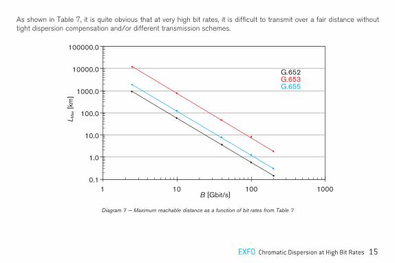
As shown in Table 7, it is quite obvious that at very high bit rates, it is difficult to transmit over a fair distance without tight dispersion compensation and/or different transmission schemes.

100000.0

10000.0

1000.0

100.0

10.0

1.0

0.11

G.652G.653G.655

10

L Max [k

m]

B [Gbit/s]100 1000

Diagram 7 − Maximum reachable distance as a function of bit rates from Table 7


6. Dispersion impairment and compensationIf the link is made of many spans, the situation shown in Diagram 8 repeats itself for each span. At each span node, compensation can be provided up to the receiver end, where a final compensation is applied with a certain residual value, as shown in Diagram 9.

Chromatic dispersion must therefore be compensated by applying an equal amount of negative CD (for ITU-T G.652 type fiber), as shown in Diagram 9.

In a non-WDM system, compensation is applied at the receiver end; whereas, in a WDM system, compensation is usually applied to the amplifiers (see Diagrams 10 to 12) as well as at the receiver end.

Diagram 11 illustrates the case where static CD-compensation modules (DCM) are used with inline EDFAs and at the receiver end in a dense wavelength-division multiplex (DWDM) system. The example shows a static CD compensation scheme, in which a fixed value of negative CD is applied to the DCM. This applies specifically to CD compensation on OC-192/STM-64 line rates and lower. For very high bit rate systems, a dynamic CD compensation scheme will have to be applied to each receiver in a DWDM multiplexer, as shown in Diagram 12.

Diagram 8 – Relationship between spectral and distance variation in chromatic dispersion (3 WDM channels are

used in this example)D

(ps/

nm)

Beg

inni

ng o

f sec

tion

End

of s

ectio

n

D (p

s/nm

-km

)

λ (nm)λ0/ω0

Distance (km)

0

+

–


Diagram 9 – Attenuation, chromatic dispersion and compensation as a function of distance in a WDM system using dispersion-compensating fiber inside amplifiers


Diagram 10 – Location of a dispersion compensation module inside an amplifier (EDFA)

Diagram 11 – Dispersion compensation modules used in a DWDM system


Diagram 12 – Static and adaptive dynamic dispersion compensation in a DWDM system

6.1 Dispersion compensation

There are several passive and active ways to compensate for CD:

(1) Passive CD-compensation techniques:› CD-compensating fiber (DCF)

› Fiber CD mapping

› Fiber Bragg grating (FBG)

› Higher-order-mode (HOM) fiber

› Virtually imaged phased array (VIPA)

› CD-supported transmission such as CD mapping

› Holey fiber

(2) Active CD-compensation techniques:› Nonlinear effect (NLE) and nonlinear-conditioned

transmissions such as soliton transmission

› Pre-conditioning such as pre-chirping

› Electronic signal processing › Phase correction › Decision-level feedback › Forward error correction (FEC)

› Spectral inversion (i.e., inverting of spectral components typically at mid-system range)


6.2 Dispersion-compensating fiber in a WDM system

To illustrate dispersion compensation, let’s examine a WDM system and its response to CD compensation using DCF. The system consists of:

› Number of WDM channels: 4

› Channel spacing: 200 GHz

› Modulation format: unchirped NRZ

› Link distance: 400 km

› Location of inline amplifiers and DCF: devices used together at every 80 km

Table 8 – Example of dispersion values and slopes for the channel plan

The DCF is chosen in order to obtain exact compensation; first on channel 1 and then on channel 3.

Channel Number ν (THz) l (nm)

D for l0 [ps/(nm•km)] S = dD/dl [ps/(nm2•km)]D (1300 nm) D (at mid point) D (1324 nm) %Δ

1 193.500 1549.31503 +18.166 +17.488 +16.810 4% 0.05906

2 193.300 1550.91804 +18.258 +17.583 +16.907 4% 0.05892

3 193.100 1552.52438 +18.351 +17.677 +17.004 4% 0.05877

4 192.900 1554.13405 +18.443 +17.772 +17.101 4% 0.05862

DCF -- -- -- –80 -- -- –0.2

G.652 -- 1550 -- +17 -- -- 0.056


Diagram 13 (a) shows the CD progression from one link section to the other until the end of the link, when exact compensation is applied to channel 1. Diagram 13 (b) is the same as 13 (a) except that the exact compensation is applied to channel 3.

While the CD and DCF slopes are fixed values, those of the wavelengths differ (see Table 8). This means that each channel experiences different CD levels, and compensation is not applied equally. The residual CD of each channel increases with distance.

Diagram 13 represents two compensation strategies; it shows the progression of the residual CD only (not CD values) as a function of distance for each channel when exact compensation is applied to channel 1 or channel 3. The dash line shows the overall link compensated CD for each channel. It simply means that, at that particular level of CD, the channel will not be able to transmit any further without experiencing CD impairment. The CD value of the compensated channel has been set to 0.2 ps/nm for each section of the link (the CD compensation must not target zero D).

1400

1200

1000

800

600

400

200

00 80 160 240 320 400

Dis

pers

ion

D•L

[ps/

nm]

Distance L [km]

Ch 1Ch 2Ch 3Ch 4

1300

1100

900

700

500

300

100

-1000

Ch 1Ch 2Ch 3Ch 4

80 160 240 320 400

Dis

pers

ion

D•L

[ps/

nm]

Distance L [km]

Diagram 13 – Progression of dispersion with compensation applied to single channel

(a) Compensation of channel 1 at 0.2 ps/nm (b) Compensation of channel 3 at 0.2 ps/nm


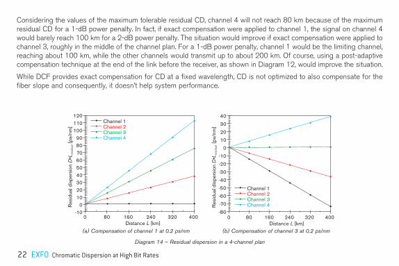
Considering the values of the maximum tolerable residual CD, channel 4 will not reach 80 km because of the maximum residual CD for a 1-dB power penalty. In fact, if exact compensation were applied to channel 1, the signal on channel 4 would barely reach 100 km for a 2-dB power penalty. The situation would improve if exact compensation were applied to channel 3, roughly in the middle of the channel plan. For a 1-dB power penalty, channel 1 would be the limiting channel, reaching about 100 km, while the other channels would transmit up to about 200 km. Of course, using a post-adaptive compensation technique at the end of the link before the receiver, as shown in Diagram 12, would improve the situation.

While DCF provides exact compensation for CD at a fixed wavelength, CD is not optimized to also compensate for the fiber slope and consequently, it doesn’t help system performance.

120110100

908070605040302010

0-10

0 80

Res

idua

l dis

pers

ion

D•L

resi

dual [p

s/nm

]

Distance L [km]240160 320 400

Channel 1Channel 2Channel 3Channel 4

40

30

20

10

0

-10

-20

-30

-40

-50

-60

-70

-800 80

Res

idua

l dis

pers

ion

D•L

resi

dual [p

s/nm

]

Distance L [km]240160 320 400

Channel 1Channel 2Channel 3Channel 4

Diagram 14 – Residual dispersion in a 4-channel plan

(a) Compensation of channel 1 at 0.2 ps/nm (b) Compensation of channel 3 at 0.2 ps/nm


6.3 Maximum CD deviation

Chromatic dispersion deviation is also an important parameter at very high bit rate transmissions that must be considered when applying CD compensation. At installation, the measured CD value of the optical path is used to determine the magnitude of the compensation within the Rx. When defining the actual value of the optical path and the actual compensation value within the Rx, at any time after installation, they are required to be below the maximum residual CD.

The maximum CD deviation is the maximum tolerated difference between the actual value of the optical path (from Tx to Rx) and the path value determined at the time of installation.

This value varies between non-return-to-zero (NRZ) and return-to-zero (RZ) modulation and between the various RZ duty cycles.

It is quite challenging to specify the maximum tolerable residual CD in a very high bit rate system because several variables must be considered:

› Tx optical power output

› Modulation format

› Inline amplifier gain and saturation power level

› Inline amplifier design (number of pumps and number of stages)

› Compensation techniques

› Link distance

› Fiber type


6.4 WDM systems: tolerance to residual CD

In WDM transport systems, the CD slope of the fiber (and link) must be taken into account because the CD spectral variation is nonlinear (i.e., a different CD for each WDM channel), as shown in Diagram 6.

Each WDM channel is characterized by a different CD value.

At the moment, it is still quite difficult to find CD-compensation devices that can compensate for the CD slope as well (i.e., compensating each individual channel of a DWDM channel plan with a broadband-compensating device in order to get a constant CD independent of the planned wavelengths).

Consequently, when using broadband CD-compensating devices such as DCFs in WDM transmission systems, the DCF may obtain exact compensation for the central channel (or any other one) in the channel plan, while the lateral ones experience a residual CD.

At this point, the maximum tolerable residual CD for each channel receiver can be evaluated. Such values establish limits for the number of channels (N), the channel spacing and the link length.

When a larger residual CD characterizes some channels, it is still possible to obtain acceptable performances through additional compensation (adaptive CD-compensation module) used after the demultiplexer and before the receiver with the optimum value for each channel. Technologies such as tunable or fixed chirped-Fiber Bragg gratings (CFBG) are useful in these cases.


7. Modulation and its influence on chromatic dispersion 7.1 Modulator influence

Selecting the most cost-effective modulation format is not easy for very high bit rate applications. It mostly depends on the modulator type, the presence or not of modulator chirp and the modulation format.

There are four basic signal properties that can be used to produce a modulation:

› Amplitude on/off keying (OOK) › Non-return-to-zero (NRZ) › Return-to-zero (RZ) › Carrier-suppressed-RZ (CS-RZ) › Single-sideband RZ (SSB-RZ)

› Phase-shift keying (PSK)

› Frequency-shift keying (FSK)

› Polarization-shift keying (PolSK)

Ensuring limited linear and nonlinear network impairments requires a strong modulation format with the following characteristics:

› A narrow optical spectrum that favors DWDM transmission with narrow channel spacing and tolerates more CD distortion.

› Constant optical power that is less susceptible to nonlinear effects such as self-phase modulation (SPM) and cross-phase modulation (XPM).

› Multiple signal levels that are more efficient than binary signals with longer symbol duration, thus reducing CD- and PMD-induced distortions.


7.2 NRZ-OOK modulation format

Diagram 16 illustrates the phase and waveform of a bit-stream transmission based on the NRZ modulation format. NRZ is typically based on on/off keying (OOK) modulation, in which the signal is intensity-modulated. When the laser signal is on, a 1 bit is produced, whereas when the laser is off, a 0 bit is produced.

The NRZ modulation format provides a relatively wide pulse in the time domain with a corresponding narrow spectrum, as seen in Diagram 17.

On the frequency axis, the width of the spectrum is not as wide (~60 GHz, FW90%M) and is not narrow enough to support DWDM channel spacing narrower than 200 GHz. Nonetheless, the wide NRZ pulse does not favor very high speed transmission and encourages phase temporal variation inside the pulse and consequently, CD impairment. The VHBR NRZ spectral and pulse widths are not prone to support very dense WDM transmissions with strong CD tolerance, especially when it comes to residual CD in an amplified system with CD compensation.

Diagram 16 – Example of NRZ format transmission

Diagram 17 – Example of a VHBR NRZ transmission spectrum

0

-10

-20

-30

-40

-50

-60

-70

-80

-90

-100

-110

-1200 -240 -180

Pow

er (d

Bm

)

Frequency (GHz)B=(Bit Period)-1

-120 -60

-B B 2B-2B

60 1200 180 240


Impairment-free VHBR transmission typically requires a shorter pulse width with sufficient OSNR, but also a narrower spectrum to accommodate DWDM transmission with narrow channel spacing. Evidently, these requirements are idealistic; in the real world, compromises must be made. Consequently, NRZ may not be optimal for very-high-bit-rate transmission and even less suitable for a DWDM scheme. This means that other modulation formats must be considered.

7.3 RZ-OOK modulation format

As shown in Diagram 3, RZ modulation is preferred to NRZ because the RZ bits use up less time in their timeslots and therefore, improve receiver sensitivity. The RZ optical signal is more tolerant to nonlinear effects than NRZ.

This characteristic of the RZ format makes the pulse width of the 1 bit narrower, allowing for some pulse broadening and in turn better CD tolerance, especially when it comes to residual CD in an amplified system with CD compensation.

However, the downside is that lower duty cycles mean a wider spectrum with less energy per pulse for RZ than for NRZ in their respective spectra (see Diagram 18), thus increasing the OSNR penalty. Increasing peak power is not a solution due to the increased risk of generating nonlinear effects while restricting DWDM transmission with narrow channel spacing. Normal RZ is therefore not an ideal solution for VHBR transport.

Diagram 18 – Difference in spectra between narrower NRZ and wider

RZ modulation formats

Pow

er

B=1/Bit Period

-2B -B B 2B0

RZ

NRZ


7.4 PSK modulation format

A potential solution for a more efficient and tolerant modulation format is to use the phase of the wave transporting the information signal and its amplitude. This approach is called phase-shift keying (PSK). Changing the polarity of the modulator voltage changes the phase response of the wave from 0 to π (+180°), as shown in Diagram 19. A phase shift of π was chosen for convenience and simplicity.

Bit 1 is transmitted by shifting the phase of the carrier by π relative to the previous carrier phase; whereas bit 0 is transmitted by a 0 or no phase shift relative to the phase in the preceding signaling interval.

In PSK, the state of each bit is determined by the state of the preceding bit. If a 0 precedes a 0, then there is no phase change. The same is true for two consecutive 1 bits. However, when a 1 follows a 0, there is a 180° or π phase shift relative to the previous carrier phase. The same applies when a 0 follows a 1. To recap, when the phase of the wave does not change, then the signal state stays the same (0 or 1). When the phase of the wave changes by π (i.e., the phase reverses), then the signal state changes.

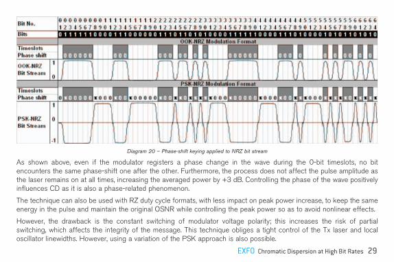
Diagram 20 illustrates the phase-change process for an NRZ bit stream, compared to no phase shift (0 phase) in NRZ-OOK transmission.

Diagram 19 – Phase shift of a wave from 0 to π

π/2 3π/4 2π0 π

π phase shift


As shown above, even if the modulator registers a phase change in the wave during the 0-bit timeslots, no bit encounters the same phase-shift one after the other. Furthermore, the process does not affect the pulse amplitude as the laser remains on at all times, increasing the averaged power by +3 dB. Controlling the phase of the wave positively influences CD as it is also a phase-related phenomenon.

The technique can also be used with RZ duty cycle formats, with less impact on peak power increase, to keep the same energy in the pulse and maintain the original OSNR while controlling the peak power so as to avoid nonlinear effects.

However, the drawback is the constant switching of modulator voltage polarity; this increases the risk of partial switching, which affects the integrity of the message. This technique obliges a tight control of the Tx laser and local oscillator linewidths. However, using a variation of the PSK approach is also possible.

Diagram 20 – Phase-shift keying applied to NRZ bit stream


7.5 Variation in the phase-shift keying modulation technique – NRZ-DPSK modulation format

A promising modulation format for VHBR transmission is differential phase-shift keying (DPSK). In DPSK, a 1 bit is transmitted with a π phase-shift between consecutive 1-1 symbols. There is no phase change for a 0 between consecutive 0-0 symbols. More importantly, the Tx is kept on even for 0 bits. In this case, the phase difference determines the value of the bit. Diagram 21 illustrates a DPSK bit stream.

RZ-DPSK is a better format because of its narrower pulse and because it maintains the advantages of the NRZ-DPSK.

Diagram 21 – Differential phase-shift keying applied to a NRZ bit stream


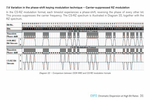
7.6 Variation in the phase-shift keying modulation technique – Carrier-suppressed RZ modulation

In the CS-RZ modulation format, each timeslot experiences a phase-shift, reversing the phase of every other bit. This process suppresses the carrier frequency. The CS-RZ spectrum is illustrated in Diagram 22, together with the RZ spectrum.

Diagram 22 – Comparison between OOK-NRZ and CS-RZ modulation formats


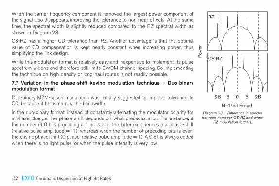
When the carrier frequency component is removed, the largest power component of the signal also disappears, improving the tolerance to nonlinear effects. At the same time, the spectral width is slightly reduced compared to the RZ spectral width as shown in Diagram 23.

CS-RZ has a higher CD tolerance than RZ. Another advantage is that the optimal value of CD compensation is kept nearly constant when increasing power, thus simplifying the link design.

While this modulation format is relatively easy and inexpensive to implement, its pulse spectrum widens and therefore still limits DWDM channel spacing. So implementing the technique on high-density or long-haul routes is not readily possible.

7.7 Variation in the phase-shift keying modulation technique – Duo-binary modulation format

Duo-binary MZM-based modulation was initially suggested to improve tolerance to CD, because it helps narrow the bandwidth.

In the duo-binary format, instead of constantly alternating the modulator polarity for a phase change, the phase shift depends on what precedes a bit. For instance, if the number of 0 bits preceding a 1 bit is odd, the latter experiences a π phase-shift (relative pulse amplitude = -1); whereas when the number of preceding bits is even, there is no phase-shift (0 phase, relative pulse amplitude = 1). A 0 bit is always coded when there is no light pulse, or when the pulse intensity is very low.

Diagram 23 – Difference in spectra between narrower CS-RZ and wider

RZ modulation formats

Pow

er

B=1/Bit Period

-2B -B B 2B0

CS-RZ

RZ


This phase-change narrows the pulse spectral width and causes the CD of opposite-phase bits to destructively interfere, thus reducing the effect of CD (see Diagram 24).

As a result, the modulator does not have to switch the phase back and forth as in PSK. This means that the pulse is less distorted, with respect to time and frequency domains.

Diagram 24 – Phase-change in a duo-binary modulation format on an NRZ bit stream


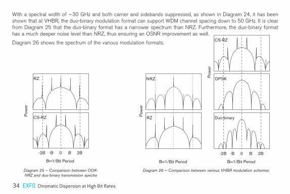
With a spectral width of ~30 GHz and both carrier and sidebands suppressed, as shown in Diagram 24, it has been shown that at VHBR, the duo-binary modulation format can support WDM channel spacing down to 50 GHz. It is clear from Diagram 25 that the duo-binary format has a narrower spectrum than NRZ. Furthermore, the duo-binary format has a much deeper noise level than NRZ, thus ensuring an OSNR improvement as well.

Diagram 26 shows the spectrum of the various modulation formats.

Diagram 25 – Comparison between OOK-NRZ and duo-binary transmission spectra

Diagram 26 − Comparison between various VHBR modulation schemes

Pow

er

B=1/Bit Period

-2B -B B 2B0

CS-RZ

RZ

B=1/Bit Period

Pow

er

RZ

NRZ

Duo-binary

DPSKPow

er

B=1/Bit Period

-2B -B B 2B0

CS-RZ


Table 9 shows the spectral width of the spectra in Diagram 26.

Table 9 – Difference in spectral width of various VHBR modulation formats

Modulation formatFWXM (GHz) NRZ RZ CS-RZ Duo-binary

X = –40 dB 40 80 90 60

X = –60 dB 100 140 140 90

X = –70 dB 210 230 220 120


Table 10 shows the limits of CD tolerance at 100 Gbit/s for several different modulation format implementations, as advertised by different system vendors.

Table 10 – Commercial implementation CD tolerances at 100 Gbit/s

Modulation formats

Parameters 100 Gbit/s OOK PSBT DPSK QPSK DQPSK PM-QPSK PM-DQPSK

Spectral efficiency bit/s/Hz 0.4 1 0.8 1.6 1.6 3 3

OSNRdB in 0.1 nm

RBW20 20 17 15.5 18 15.5 18

Dispersion tolerance Intrinsic -- -- -- -- -- -- --

PMD ps 1 1 1 2 2 2.5 2.5

CD ps/nm 15 50 12 35 35 140 140

Complexity technical L M M M H VH VH

Estimated reach km Limited by optical amplifier noise (ASE)

Relative costIncrease from

OOK-- 1.1 1.2 1.5 1.7 1.9 2.1


8. Chromatic dispersion measurementThere are two situations in which CD testing is conducted:

› Laboratory measurements on optical fibers and cables, including tests performed during R&D, engineering and manufacturing, as well as for repairs.

› Field measurements, including tests performed on deployed, cabled fibers to qualify links for upgrade to higher bit rates.

In both cases, group delay is measured as a function of wavelength; the CD, CD slope or any other orders are extrapolated from the derivative of the group delay data (with respect to wavelength). The derivative is most often calculated after the data are fitted to a mathematical model. This approach is perfectly valid because the CD of an optical fiber is deterministic and can be perfectly modeled and predicted. However, this may not always apply to the CD measurement of a link with different components presenting different CD behavior (e.g., CD, PMD, nonlinearity).

There are two basic ways to calculate CD. The first is to fit a curve on the group delay data versus wavelength and find the derivative of the fit function. This works well for a small number of known fit functions, especially for fiber.

If there is a mix of fibers, or if some components are contributing more significantly to CD, then it is preferable to calculate local CD, using local derivatives on a limited number of delay measurements over a short wavelength span, or over two neighboring wavelengths, at a time.

When preparing an experimental setup, polarization effects must be averaged out, calibrated or compensated for.


8.1 Data fitting

A CD-fitting model is available and outlines a number of fitting equations suitable for various fiber categories as shown in Table 11.

Table 11 – Optical fiber specification and dispersion fitting

Fiber Type Fiber CategoryOptical Fiber Specification

ITU-T Rec. IEC Standard Fit

SMF

Dispersion un-shiftedG.652 A/B 60793-2-50 B1.1

G.652 C/D 60793-2-50 B1.3

Dispersion shifted G.653 60793-2-50 B21550 nm region: For ≤ 35 nm intervals: quadratic. For > 35 nm intervals: 5-term Sellmeier or 4th order polynomial.

Cut-off shifted G.654 60793-2-50 B1.21550 nm region: For ≤ 35 nm intervals: quadratic. For > 35 nm intervals: 5-term Sellmeier or 4th order polynomial

Non-zero-dispersion shifted G.655 60793-2-50 B41550 nm region: For ≤ 35 nm intervals: quadratic. For > 35 nm intervals: 5-term Sellmeier or 4th order polynomial

Non-zero-dispersion shifted wideband G.656 60793-2-50 B5For > 35 nm intervals: 5-term Sellmeier or 4th order polynomial


8.2 CD test methods

There are four methods for measuring CD that have been internationally standardized:

1. Phase-shift method (PSM)

2. Differential phase-shift method (DPSM)

3. Spectral group delay in the time domain method (OTDR method)

4. Interferometric method (INTY)

These methods are standardized in ITU-T Recommendation G.650.1 and IEC standard 60793-1-42.

Since the application space for INTY is different from the other ones, we will only review PSM, DPSM and Group Delay methods here.


8.2.1 Test method – General requirementsOptical sources have essentially the same characteristics for any method. The source may be as follows:

› Laser: › Diode-laser array › Tunable laser (TLS)

› Broadband source (BBS) with wavelength selecting filter: › Raman gain from SMF with Nd:YAG laser pump › Super-LED or LED › Amplified spontaneous emission (ASE)

Super-LED and ASE sources may be combined to emit in the C+L band for wider spectral range measurements. Testing on long fibers will always ensure better reproducibility than on short ones.

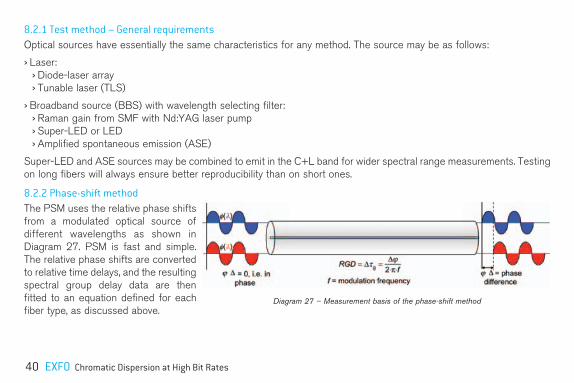
8.2.2 Phase-shift method The PSM uses the relative phase shifts from a modulated optical source of different wavelengths as shown in Diagram 27. PSM is fast and simple. The relative phase shifts are converted to relative time delays, and the resulting spectral group delay data are then fitted to an equation defined for each fiber type, as discussed above.

Diagram 27 – Measurement basis of the phase-shift method


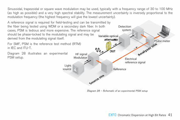
Sinusoidal, trapezoidal or square wave modulation may be used, typically with a frequency range of 30 to 100 MHz (as high as possible) and a very high spectral stability. The measurement uncertainty is inversely proportional to the modulation frequency (the highest frequency will give the lowest uncertainty).

A reference signal is required for field-testing and can be transmitted by the fiber being tested using WDM or a secondary dark fiber. In both cases, PSM is tedious and more expensive. The reference signal should be phase-locked to the modulating signal and may be derived from the modulating signal itself.

For SMF, PSM is the reference test method (RTM) in IEC and ITU-T.

Diagram 28 illustrates an experimental PSM setup.

Diagram 28 – Schematic of an experimental PSM setup

cases, PSM is tedious and more expensive. The reference signal

Diagram 28 – Schematic of an experimental PSM setupDiagram 28 – Schematic of an experimental PSM setup

Lightsource

HF signalModulator

Variable opticalattenuator

Reference

Phase meter

Electrical reference signal

DUTAnalyzer site

Source site

Variable opticalVariable opticalVariable opticalattenuatorattenuatorattenuator

DUTDUTDUT

Detectionsystem


A best fit is applied to the RGD dataset and the dispersion can be calculated from the fit using the equations listed in Table 11.

Diagrams 29 and 30 show the results obtained using the PSM.

Diagram 29 – Example of PSM test result for G.653 conventional fiber Diagram 30 – Example of PSM test result for DCF


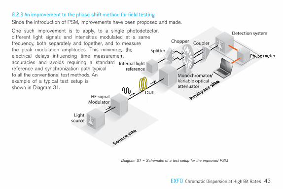
8.2.3 An improvement to the phase-shift method for field testingSince the introduction of PSM, improvements have been proposed and made.

One such improvement is to apply, to a single photodetector, different light signals and intensities modulated at a same frequency, both separately and together, and to measure the peak modulation amplitudes. This minimizes the electrical delays influencing time measurement accuracies and avoids requiring a standard reference and synchronization path typical to all the conventional test methods. An example of a typical test setup is shown in Diagram 31.

Diagram 31 – Schematic of a test setup for the improved PSM

the peak modulation amplitudes. This minimizes the electrical delays influencing time measurement

Lightsource

HF signalModulator

Monochromator/Variable optical attenuator

Phase meter

Detection system

DUTAnalyzer site

Source site

DUTDUTDUTDUT

Internal lightreference

Splitter

CouplerChopper

Monochromator/Monochromator/

Phase meterPhase meterPhase meterPhase meterPhase meterPhase meterPhase meterPhase meterPhase meterPhase meterPhase meterPhase meterPhase meterPhase meterPhase meterPhase meterPhase meterPhase meterPhase meterPhase meterPhase meterPhase meterPhase meter

Analyzer site

Analyzer site

Analyzer site

Analyzer site


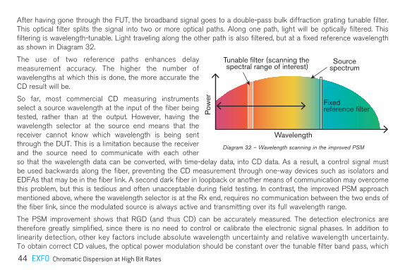
After having gone through the FUT, the broadband signal goes to a double-pass bulk diffraction grating tunable filter. This optical filter splits the signal into two or more optical paths. Along one path, light will be optically filtered. This filtering is wavelength-tunable. Light traveling along the other path is also filtered, but at a fixed reference wavelength as shown in Diagram 32.

The use of two reference paths enhances delay measurement accuracy. The higher the number of wavelengths at which this is done, the more accurate the CD result will be.

So far, most commercial CD measuring instruments select a source wavelength at the input of the fiber being tested, rather than at the output. However, having the wavelength selector at the source end means that the receiver cannot know which wavelength is being sent through the DUT. This is a limitation because the receiver and the source need to communicate with each other so that the wavelength data can be converted, with time-delay data, into CD data. As a result, a control signal must be used backwards along the fiber, preventing the CD measurement through one-way devices such as isolators and EDFAs that may be in the fiber link. A second dark fiber in loopback or another means of communication may overcome this problem, but this is tedious and often unacceptable during field testing. In contrast, the improved PSM approach mentioned above, where the wavelength selector is at the Rx end, requires no communication between the two ends of the fiber link, since the modulated source is always active and transmitting over its full wavelength range.

The PSM improvement shows that RGD (and thus CD) can be accurately measured. The detection electronics are therefore greatly simplified, since there is no need to control or calibrate the electronic signal phases. In addition to linearity detection, other key factors include absolute wavelength uncertainty and relative wavelength uncertainty. To obtain correct CD values, the optical power modulation should be constant over the tunable filter band pass, which

Wavelength

Tunable filter (scanning the spectral range of interest)

Sourcespectrum

Pow

er Fixedreference filter

Diagram 32 – Wavelength scanning in the improved PSM


is not the case, since the BBS has a spectral power distribution. As it goes through the DUT, the power modulation distribution changes. This distribution should be measured and used to compute the exact central wavelength of the filtered light to compensate for the power modulation line shape. This technique lends itself naturally to this type of compensation. One of the signals used to compute delays is the filtered tunable optical power modulation level. The power modulation attenuation curve can be measured at the same time as the delays. This makes it possible to compensate for the power modulation distribution.

8.2.4 Differential phase-shift method (DPSM)DPSM uses two simultaneous modulated light source wavelengths coupled into the fiber being tested. Using a dual-detection system to simultaneously record the two wavelength signals is essentially the only difference between DPSM and PSM. Diagram 34 illustrates a DPSM test setup.

The phase of the light exiting the fiber at one wavelength is compared to the phase of the light exiting at another closely spaced wavelength. Average CD over the interval between the two wavelengths is determined from the differential phase shift, wavelength interval and fiber length. The wavelength spacing between the differential phase measurement data is typically in the range of 2 to 20 nm.

The CD coefficient, at a wavelength medial to the two test wavelengths, is assumed to be equal to the average CD over the interval between said wavelengths. The resulting CD data are then fitted to an equation defined for each fiber type, as per other methods.

Diagram 33 – RGD and CD coefficient field measurements of a G.653 fiber in the C-band using the improved PSM


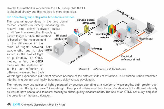
Overall, this method is very similar to PSM, except that the CD is obtained directly and this method is more expensive.

8.2.5 Spectral group delay in the time domain methodThe spectral group delay in the time domain method consists in directly measuring the relative time delays between pulses of different wavelengths through a known length of fiber. The method is based on the measurement of the difference in the “time of flight” between wavelengths and is also known as the time-of-flight or pulse-delay or OTDR method. In fact, the OTDR measures the distance up to the last reflection at different wavelengths. Each wavelength experiences a different distance because of the different index of refraction. This variation is then translated into the time domain and finally, becomes a delay versus wavelength.

The method may use pulses of light generated by sources operating at a number of wavelengths, both greater than and less than the typical zero-CD wavelength. The optical pulses must be of short duration and of sufficient intensity as well as have spatial and temporal stability to obtain quality measurements. The use of an OTDR obviously simplifies the selection of the pulse duration.

Diagram 34 − Schematic of a DPSM test setup

of different wavelengths through a known length of fiber. The method

Diagram 34 − Schematic of a DPSM test setup

of the difference in the “time of flight” between wavelengths and is also known as the time-of-flight or pulse-delay or OTDR method. In fact, the OTDR measures the distance up to the last reflection at

Lightsource

HF signalModulator


Reference

Phase meter

Electrical reference signal

DUT

Analyzer site

Source site

The spectral group delay in the time domain Variable opticalVariable optical

attenuator

DUTDUT

Detectionsystem

ReferenceReference

Variable opticalattenuatorattenuator

DUT Wavelengthselector

Detection

ReferenceReferenceReferenceReference

DetectionDetectionDetectionDetectionDetectionDetectionDetectionsystemsystemsystem

WavelengthWavelengthselector

DetectionDetectionDetectionDetectionDetection


A delay generator, triggered by the optical source, provides a delayed trigger signal to the sampler for the purpose of compensating for the differences in propagation delay between the test and reference specimens. The delay times must be stable throughout the duration of the measurement; jitter and drift must be much shorter than the pulse width. Since an OTDR already integrates such complex electronics, the OTDR method becomes a very simple and low-cost method.

A set of measurements is taken through a short reference fiber and these reference data are subtracted from data taken from the fiber under test to obtain relative spectral group delay. The resultant spectral group delay data are then fitted into an equation defined for each fiber type as per other methods.

The linear detection system uses a high-frequency sampler, which is capable of displaying the relative arrival time of the optical pulses on a calibrated time scale. An optical attenuator may be used to maintain constant signal amplitude. The same applies to the detection electronics used in the OTDR method, as is the case for the modulator and trigger electronics.

Schematic of the OTDR setup

Diagram 35 – Spectral group delay in the time domain method

A set of measurements is taken

data are subtracted from data taken from the fiber under test to obtain relative spectral group delay. The resultant spectral group delay data are then fitted into an equation defined for each fiber type

Pulse laser source

Source/analyzer sitefitted into an equation defined for each fiber type

The linear detection system uses a high-frequency

resultant spectral group delay data are then fitted into an equation defined for each fiber type

laser sourcelaser source

Source/analyzer site

The linear detection system uses a high-frequency sampler, which is capable of displaying the relative arrival time of the optical pulses on a calibrated time scale. An optical attenuator may be used to maintain constant signal

The linear detection system uses a high-frequency



Detectionsystem

Time delaygenerator

Pulse wavelength analyser


DUTDUTDUT


Diagram 35 illustrates a test setup for the spectral group delay in the time domain (time-of-flight/OTDR) method.

Diagram 36 illustrates the operating principle of the OTDR method.

The dispersion coefficient is obtained using the best-fit values of the appropriate Sellmeier coefficients and calculating CD or other parameters as required.

Diagram 37 illustrates the result obtained by the OTDR method for a typical SMF of G.653 type with a length of 25 km (l0 = 1553.405 nm).

With the OTDR, CD is computed using the difference in distance to the last event. The accuracy of the measurement depends on the ability to measure the last reflection.

The best advantage of the OTDR method is that the measurement is performed at a single end. This typically has a huge impact on the cost of operation.

Most OTDRs use only several wavelengths in the entire fiber spectral window (>300 nm). The fit equation recommended for any type of fiber is a 5-term Sellmeier equation, which requires at least 5 points to be resolved. Fewer points may be used, but this will require some assumptions.

Diagram 36 – Operating principle of the OTDR method

The best advantage of the OTDR method is that

Most OTDRs use only several wavelengths in the 300 nm). The fit

equation recommended for any type of fiber is a

Pulse laser source

OTD

R si

gn

al


5 points to be resolved. Fewer points may be used, but this

laser sourcelaser source



Detectionsystem

Time delaygenerator

Timet1

λ1 λ2 λ3

1st event 2nd event End of fiber

t2

Variableoptical attenuator

Pulse wavelength analyser

t1 t2

DUT


Based on fiber attenuation, the more attenuated wavelength signals (1310 nm or close to the water peak such as 1410 nm, on a conventional G.652 fiber) will disappear after 70 to 80 km (dynamic range of about 30-35 dB at best), leaving the analysis with 3 points over the entire wavelength range (for CD approximation). When some wavelengths disappear, other readings are drowned out by the noise at the end of the trace. Since measurement repeatability is a function of OSNR, the average time required to obtain an acceptable repeatability, not accuracy, will increase rapidly depending on the length of the fiber. Acquisition time may increase up to 10 min. per trace (typically 40 min. total). The limiting distance may then be estimated as 70 km. Conversely, the shorter the distance, the more difficult the measurement becomes. In fact, an OTDR will show strong limitations due to its clock, synchronization and pulse repeatability; and this may ultimately lead to a degradation of the measurement on short fiber. The minimum distance may therefore be estimated to be around 10 km.

The uncertainty depends on the shape and the width of the pulse and the number of different lasers (number of wavelength data points). Although this method provides better spatial resolution, short pulses will spread and distort, making the exact arrival time difficult to determine. This simple technique is also relatively inaccurate when used as is. It therefore needs to be enhanced to arrive at an uncertainty of the same level as PSM. For example, more wavelengths or a tunable laser can be used, but the required investment quickly brings the OTDR method to roughly the same level of relative capital cost as the PSM. However, considering that it is single-end, the OTDR method still generates cost savings when it comes to operation.

40

20

0

-20

-40

-60

-80

1510

1520

153

0

154

0

155

0

156

0

1570

158

0

159

0

1600

1610

Gro

up d

elay

coe

ffici

ent (τ g

/L) [

ps/k

m]

Wavelength [nm]Diagram 37 − Relative group delay measured by the OTDR method


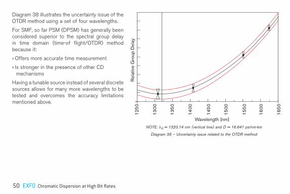
Diagram 38 illustrates the uncertainty issue of the OTDR method using a set of four wavelengths.

For SMF, so far PSM (DPSM) has generally been considered superior to the spectral group delay in time domain (time-of flight/OTDR) method because it:

› Offers more accurate time measurement

› Is stronger in the presence of other CD mechanisms

Having a tunable source instead of several discrete sources allows for many more wavelengths to be tested and overcomes the accuracy limitations mentioned above.

125

0

1300

135

0

1400

145

0

1500

155

0

1600

165

0

Rel

ativ

e G

roup

Del

ay

Wavelength [nm]

NOTE: l0 = 1320.14 nm (vertical line) and D = 16.641 ps/nm·km

Diagram 38 – Uncertainty issue related to the OTDR method


9. Chromatic dispersion testing in coherent systemsThe demand for increased bandwidth is constant, and to avoid investing huge amounts in new systems, most operators, if not all of them, are looking to re-use their existing fiber infrastructure. This, however, poses a problem because the standard train of 1s and 0s, called on-off keying (OOK), simply can’t be pushed any further on most of the installed bases.

To resolve this issue, system vendors have introduced higher bits per symbol modulation formats. One of the most popular ones is called DP-QPSK: dual polarization quadrature phase-shift keying. Unfortunately, direct detection used with OOK doesn’t work with such modulation formats. For this reason, these DP-QPSK are often referred to as coherent detection systems, which is a way to retrieve information despite a fiber’s physical impairments, such as chromatic dispersion and polarization mode dispersion.

While it is true that these systems offer more tolerance against these impairments, they are not immune to them. For example, the typical marketing specification for average PMD tolerance is 25 ps. While this is true in theory, for a real-world system, this doesn’t mean much because such a system might already have issues at 10 ps; the exact same limiting value as 10 Gbit/s. The issue is that at NRZ, this higher temporary PMD value only causes a few bit errors, which in many cases can be compensated by the FEC. In a coherent system, this high PMD can cause the whole DSP to fail, which will result in a complete service outage that may last only a few seconds or require a complete reboot.

Even though it’s not perfect, a coherent system is much more robust and reliable, and it’s the only cost-effective way to gain significant bandwidth as service providers look to upgrade to 100 GigE.

Since they do provide robustness and reliability and can tolerate greater physical impairments, coherent systems are deployed on much longer routes, typically backbone or core fiber spans. However, this means that extra amplification is required. To keep the upgrade to these new systems in the infrastructure to a minimum and ensure a financially viable solution, some limitations must be considered. The main limitation of DP-QPSK and coherent detection is optical signal-to-noise ratio (OSNR). These system upgrades will require higher OSNR. Since these fiber spans will be very long and the signal will need to be amplified or pumped to travel that extra distance, signal boosts need to be obtained with


low-noise amplification piggy-backed on current ones. Raman amplification is therefore very popular in most coherent systems because the goal of the Raman is to increase optical power at the EDFA input in order to improve OSNR, whether they are green field or brown field.

9.1 Raman gainWhile EDFA uses a specially doped fiber as an amplification medium, Raman is gain that is distributed throughout the transport fiber itself. Raman pump can be either co-propagating (i.e. connected to the Tx port and directly boosting the signal at the Tx port), or counter-propagating (i.e. connected to the Rx port and pumped energy is coupled upstream to the traffic), giving more amplification to the signal when it becomes weaker, instead of directly at the Tx. The OSNR can be improved by as much as 11 dB, which is critical to coherent signal deployment.

Since Raman uses the transmission fiber as the amplifying medium, fiber quality is a major consideration. Gain performance is highly dependent on fiber plant, which includes the loss. Splice loss, Fresnel reflections and fiber attenuation are taken into account during the engineering stage. Poor splice loss and patch panel quality can impact the achievable gain by reducing the Raman power that gets into the fiber. Macrobends in the patch panel area have also become a source of concern. Due to the high power pumped by the Raman, dirty or poorly mated connectors have proven to be an issue as well. Cleaning is needed.

EDFAOAM Co-prop Raman Counter-prop Raman

EDFAOAM

Fiber span

Diagram 39 – Raman amplification can be either co-propagating or counter-propagating


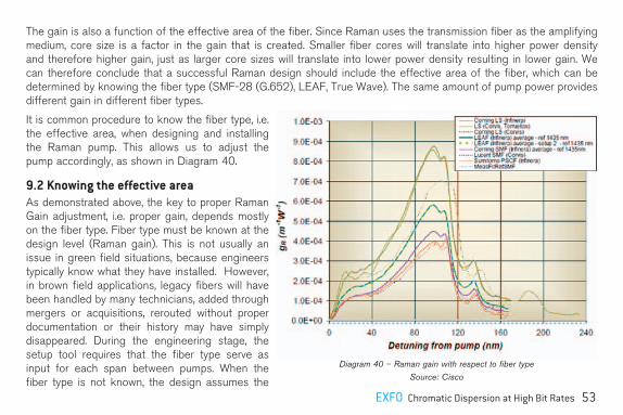
The gain is also a function of the effective area of the fiber. Since Raman uses the transmission fiber as the amplifying medium, core size is a factor in the gain that is created. Smaller fiber cores will translate into higher power density and therefore higher gain, just as larger core sizes will translate into lower power density resulting in lower gain. We can therefore conclude that a successful Raman design should include the effective area of the fiber, which can be determined by knowing the fiber type (SMF-28 (G.652), LEAF, True Wave). The same amount of pump power provides different gain in different fiber types.

It is common procedure to know the fiber type, i.e. the effective area, when designing and installing the Raman pump. This allows us to adjust the pump accordingly, as shown in Diagram 40.

9.2 Knowing the effective areaAs demonstrated above, the key to proper Raman Gain adjustment, i.e. proper gain, depends mostly on the fiber type. Fiber type must be known at the design level (Raman gain). This is not usually an issue in green field situations, because engineers typically know what they have installed. However, in brown field applications, legacy fibers will have been handled by many technicians, added through mergers or acquisitions, rerouted without proper documentation or their history may have simply disappeared. During the engineering stage, the setup tool requires that the fiber type serve as input for each span between pumps. When the fiber type is not known, the design assumes the

Diagram 40 – Raman gain with respect to fiber typeSource: Cisco


fiber type to be SMF-28, G.652. What is the impact of not knowing the effective area in the fiber? The Raman gain could be incorrectly engineered.

As stated earlier, the same amount of pump power provides different gain in different fiber types. Raman applications include longhaul, multi-span systems. The setup requires that spans be configured sequentially from the node where the Tx signals originate and then, from pump to pump along the span. This will include dB loss, fiber length and fiber type. If the span is bidirectional, Raman pumps will be scripted in one direction until the signal reaches the end and then scripted in the opposite direction. If the design was incorrectly done for a specific fiber type because of poor or no documentation or because the wrong type of fiber between the pump sites was assumed, turn up could be shut down; meaning additional engineering time. Most of system turn-ups require many technicians at the pump sites during short maintenance windows. Repeat truck rolls can be costly and time-consuming. In some instances, multiple fiber types can be used to connect the Tx and Rx in the network. This too needs to be considered because the design tools do not currently allow for mixed fiber type input, but the identification of the dominant fiber type is required in the first 50 km.

9.3 CD TestingAs stated at the beginning of this paper, tolerance to chromatic dispersion in coherent systems is very high, so compensation is not necessarily required. However, a chromatic dispersion test can provide much more insight, especially a single-ended one, which also measures fiber length.

Chromatic dispersion analyzers measure the total chromatic dispersion of the fiber as a function of wavelength, which also includes the CD slope. With these parameters, the CD test set calculates a Lambda-Zero—the wavelength where no dispersion occurs.

Plus, every fiber type has a signature, which includes a CD coefficient, CD slope and Lambda-Zero.

Chromatic dispersion coefficient is the CD by unit of length, in kilometers. This implies that the exact fiber length is known. When the CD unit is a single-ended one, reflectometry can be used to measure length, and therefore, obtain the coefficient.


Table 12 – Examples of fiber signatures

Once an operator has tested the fiber span for chromatic dispersion, the overall ps/nm may not be needed for the coherent signal. However, the overall ps/nm may be used with the fiber length determined by the single-ended dispersion analyzer to calculate the ps/nm/km at 1550 nm. It can also be used with the dispersion slope and the lambda zero to determine fiber type. For example, a large service provider deploying 100 GigE coherent detection signals, which include a counter-propagating Raman pump, must test the 40 km span for loss, ORL and chromatic dispersion. The CD measurements yield 4.48 ps/nm/km and a lambda zero at 1500.27 nm. Based on the chart above, this 40 km span is most probably Corning E-LEAF fiber and the data in the design tool suggests turning up the Raman pump. If the fiber type was unknown, the design tool for the pump would have assumed a standard single mode fiber and there would have been a higher gain than expected possibly causing four-wave mixing (FWM) or other non-linear effects.

Fiber Type Abbreviation Lambda ZeroDispersion @1550

ps/(nm*km)Slope @ 1550 nM

(ps/(nm*nm)*km)

Standard single-mode SM 1300-1324 nM 16-18 (17 typical) ~.056

Corning LS LS ~1570 –3.5 to –0.1 (–1.4 typical) ~.07

Dispersion Shifted DS ~1550 ~0 ~.07

True Wave Classic TW-C ~1500 0.8-4.6 (2 typical) ~.06

True Wave Plus True Wave Plus ~1530 1.3-5.8

True Wave Reduced Slope TW-RS ~1460 2.6-6 (4 typical) <.05 (.045 typical)

Corning E-LEAF E-LEAD ~1500 2-6 (4 typical) ~.08

Alcatel Teralight Teralight ~1440 5.5-9.5 (8 typical) ~.058

True-Wave Reach TW-Reach ~1405 5.5-8.9 (7-8 typical) <0.45


A good portion of today’s DWDM networks contain Raman pumps. Raman pumps require the fiber type to be known at the system design and optimization stages to be able to determine the proper gain. A very effective way to do this is to measure the chromatic dispersion parameters of the fiber, on a span per span basis. The advantage of single-ended testers is two-fold here: they automatically measure the fiber length, and the CD coefficient. This removes the need to shoot with an OTDR or to rely on (potentially erroneous) data. Moreover, since multi-spans over great distances must be characterized, doing this with end-to-end test sets requires much more effort: not just 2 people, but 2 people that need to travel and synchronize their presence.

Full fiber characterization, including chromatic dispersion, remains an important step when designing systems using legacy fiber. It’s just as important in the design of coherent-detection based systems, but for entirely new reasons. The data collected from the tests can help save days of work, increase time to revenue and significantly decrease your operating expenses.

AcknowledgementsThis guide would not have been possible without the enthusiasm and teamwork of EXFO staff, particularly the hard work and technical expertise of the Product Line Management team.

No part of this guide may be reproduced in any form or by any means without the prior written permission of EXFO.

Printed and bound in Canada

ISBN 978-1-55342-100-9 Legal Deposit-National Library of Canada 2012Legal Deposit-National Library of Quebec 2012

©20

12 E

XFO

inc.

All

right

res

erve

d. P

rinte

d in

Can

ada

12/0

8 20

1206

09

SA

P 1

0637

46

For details on any of our products and services, or to download technical and application notes, visit our website at www.EXFO.com.

chromatic dispersion at high bit rates - ccontrols.ch · this pocket guide provides a comprehensive...

Documents